45

Chapter 4

FUZZY LOGIC CONTROLLER DESIGN 4.1 Introduction

This chapter presents an overview of fuzzy logic evolution and Fuzzy Logic Controller

[FLC] engineering developments. FLC development current trends are also reviewed. Finally the

design and implementation methodology of the Mamdani type fuzzy Proportional-Integral (PI)

controller, implemented in this research for acceleration waveform amplitude control of an

electrodynamic shaker system, is presented by deriving its structure from conventional PI

controller. Detailed mathematical formulation and the resulting incremental control actions are

formulated computed and have been presented in this chapter.

4.2 Overview of fuzzy logic development

The idea of fuzzy sets was born in July 1964. It was originated by Lofti A. Zadeh, Professor

in the department of electrical engineering and computer science at University of California,

Berkeley. Professor Zadeh believed that all real-world problems could be solved with efficient,

analytical methods and/or fast electronic computers. In this direction, he has made significant

contributions in the development of system theory [e.g. the state variable approach to the solution

of simultaneous differential equations] and computer science. In early 1960s, however, he began to

feel that traditional system analysis techniques were too precise for many complex real-world

problems. In a paper, in 1961, he mentioned that a different kind of mathematics, the mathematics

of fuzzy quantities, was needed for most practical cases. A priori data as well as the criteria by

which the performance of a man-made system is judged are far from being precisely specified or

having accurately known probability distributions. The idea of grade of membership, which is a tile

concept that became the backbone of fuzzy set theory, occurred to him then. This important event

46

led to the publication of his seminal paper on fuzzy sets in 1965 and the birth of fuzzy logic

technology [Zadeh, 1965; Zadeh, 1972; Zadeh, 1972; Zadeh, 1977; Zadeh, 1988; Zadeh, 1996].

Even though there was strong resistance to fuzzy logic initially, many researchers around

the world became Zadeh's followers. While Zadeh continued to broaden the foundation of fuzzy set

theory, scholars and scientists in a wide variety of fields - ranging from psychology, sociology,

philosophy and economics to natural sciences and engineering were exploring this new paradigm

during the first decade after the birth of fuzzy set theory. Important concepts introduced by Zadeh

during this period include fuzzy multistage decision-making, fuzzy similarity relations, fuzzy

restrictions, and linguistic hedges. Other contributions include R. E. Bellman's work [with Zadeh]

on fuzzy multistage decision making [Bellman & Zadeh, 1970], G. Lakoff's work from a linguistic

view [Lakoff, 1973], J. A. Goguen's work on the category theoretic approach to fuzzify

mathematical structure [Goguen, 1969; Goguen, 1975], L. J. Kohout and B. R. Gaines on the

foundation of fuzzy logic [Gaines, 1976; Kohut, 1976], the work on fuzzy measures by R. E. Smith

and M. Sugeno [Smith, 1970; Sugeno, 1975], Meseguer's work on fuzzified algebraic and

topological systems [Meseguer & Sols, 1975], C. L. Chang's work on fuzzy topology [Chang,

1968], Dunn work on fuzzy clustering [Dunn, 1973], C. V. Negoita's work on fuzzy information

retrieval [Negotia, 1969; Negotia & Ralescu, 1974; Negotia & Flondor, 1976], the work by M.

Mizumoto and K. Tanaka on fuzzy automata and fuzzy grammars [Mizumoto, 1971; Mizumoto,

Toyoda & Tanaka, 1969; Mizumoto & Tanaka, 1976; Mizumoto & Zimmermann, 1982], A.

Kandel's work on the fuzzy switching function [Kandel, 1973; Kandel, 1974], and H. J.

Zimmermann's work on fuzzy optimization [Zimmermann, 1975]. During the first decade, many

mathematical structures were fuzzified by generalizing the underlying sets to be fuzzy. These

structures include logics, relations, functions, graphs, groups, automata, grammars, languages,

algorithms, and programs.

In the late 1970s, a few small university research groups on fuzzy logic were established in

Japan. Professor T. Terano and Professor H. Shibata from Tokyo University led one such group. A

47

second research group in the Kanasai area was led by Professor K. Tanaka from Osaka University

and Professor K. Asai from of the Osaka Prefecture University. An important milestone in the

history of FLC was established by Assilian and E. H. Mamdani in the United Kingdom in 1974.

They developed the first FLC, which was for controlling a steam generator. Initially, they compared

learning algorithms for adaptive control of a nonlinear, multi-dimensional plant for a physical

steam engine. They found that many learning schemes even failed to begin to converge on a

reasonable time scale. A fuzzy linguistic method was developed to prime the learning controller

with an initial policy to speed the adaptation. The verbal statements of engineers were transcribed

as fuzzy rules and were used under fuzzy logic to form a control policy. The performance of these

fuzzy linguistic controllers was so good in their own right, however, they became focal point to a

range of studies that subsequently took place. As early as 1975, E. H. Mamdani and, Baaklini

already showed that fuzzy control rules may be tuned automatically by fuzzy linguistic adaptive

strategies.

In 1976, the first industrial application of fuzzy logic was developed by M/S Blue Circle

Cement and M/S SIRA in Denmark. The system was a cement kiln controller that incorporates the

‘know-how’ of experienced operators to enhance the efficiency of a clinker through smoother

grinding. The system went to operation in 1982. After few years of persistent research,

development, and deployment efforts, Seiji Yasunobu and his colleagues at Hitachi put a fuzzy

logic-based automatic train operation control system into operation in Sendai city's subway system

in 1987. Another early successful industrial application of fuzzy logic is a water-treatment system

developed by M/S Fuji Electric. The development of water treatment systems enabled Fuji Electric

to introduce the first Japanese general-purpose FLC [named FRUITAX] into the market in 1985.

After a successful demonstration of these approaches, it took years for both projects to be deployed

in real-world operation due to various concerns about this new technology. Also these two

applications became the major "success stories" of fuzzy logic technology in Japan. Consequently,

many more Japanese engineers and companies started to investigate fuzzy logic applications.

48

The fuzzy boom in Japan was a result of the close collaboration and technology transfer

between universities and industries. In 1988, the Japanese government launched a careful feasibility

study about establishing national research projects on fuzzy logic involving both universities and

industry. Two large-scale national research projects were established by two agencies - the Ministry

of International Trade and Industry [MITI] and the Science and Technology Agency [STA]. The

project established by MITI was a consortium called the Laboratory for International Fuzzy

Engineering Research [LIFE], which involved 50 companies. M/S Matsushita Electric Industrial

[also known as M/S Panasonic outside Japan] was the first to apply fuzzy logic to a consumer

product, a shower head that controlled water temperature, in 1987. In late January 1990, Matsushita

Electric Industrial named their newly developed fuzzy controlled automatic washing machine

"Asai-go Day Fuzzy" and launched a major commercial campaign for the "fuzzy" product. This

campaign turned out to be a successful marketing effort not only for the product, but also for the

fuzzy logic technology. A foreign word pronounced "fuzzy" was thus introduced to Japan with new

meaning - intelligence. Many other home electronics companies followed Panasonic's approach and

introduced fuzzy vacuum cleaners, fuzzy rice cookers, fuzzy refrigerators, and others. This resulted

in a fuzzy vogue in Japan. As a result, consumers in Japan recognized the Japanese word "fuzzy,"

which won the gold prize for a new word in 1990.

This fuzzy boom in Japan triggered a broad and serious interest in this technology in

Europe, and, to a lesser extent, in the United States, where fuzzy logic was invented. Several major

European companies formed fuzzy logic task forces within their corporate research and

development divisions. They include M/S SGS -Thomson of Italy, M/S Siemens, M/S Daimler-

Benz, and M/S Klockner-Moeller in Germany. In the United States, the M/S General Electric

Corporate Research Division and M/S Rockwell International Science Center have both developed

advanced fuzzy logic technology as well as their industrial applications.

Fuzzy logic has found applications in other areas also. The first financial trading system

using fuzzy logic was Yamaichi Fuzzy Fund. It handles 65 industries and a majority of the stocks

49

listed on Nikkei Dow and consists of approximately 800 fuzzy rules. Rules are determined monthly

by a group of experts and modified by senior business analysts as necessary. The system was tested

for two years, and its performance in terms of the return and growth exceeds the Nikkei average by

over 20 percent. The system recommended ‘sell’ 18 days before the black Monday in 1987 and it

went into commercial operation in 1988.

The development of fuzzy systems in the early days required the manual tuning of the

system parameters based on observing system performance. This drawback has become one of the

major criticisms of fuzzy logic. Even though E. H. Mamdani and Baaklini introduced self-adaptive

FLC as early as 1975, the most common citation of the first work in this area is a paper by T. J.

Procyk and E. H. Mamdani published in 1979 [Procyk & Mamdani, 1979]. This was followed by

Japanese researchers in the 1980s. T. Takagi and his advisor M. Sugeno [Takagi & Sugeno, 1985]

together took an important step by developing the first approach for constructing [not tuning] fuzzy

rules using training data. Their approach developed fuzzy rules for controlling a toy vehicle by

observing how a human operator controlled the vehicle. Even though this important work did not

gain as much immediate attention as it did later, it laid the foundation for a popular subarea in fuzzy

logic, which is now referred to as fuzzy model identification of the 1990s.

Another trend that contributed to research in fuzzy model identification is the increasing

visibility of neural network research in the late 1980s. Because of certain similarities between

neural networks and fuzzy logic, researchers began to investigate ways to combine the two

technologies. The most important outcome of this trend is the development of various techniques

for identifying the parameters in a fuzzy system using neural network learning techniques. A

system built this way is called a neuro-fuzzy system. Bart Kosko has been known for his

contribution to neuro-fuzzy systems [Kosko, 1992]. The combination of the two techniques has led

to many new developments getting benefits from each of the methods. The other work in this has

been done by [Zimmermann, 1991; Yager & Filev, 1994; Zilouchian & Jamshidi, 2001].

50

The 1990s has been an era of new computational paradigm. In addition to fuzzy logic and

neural network, a third nonconventional computational paradigm has also become popular –

evolutionary computing, which includes Genetic Algorithms (GA), evolutionary strategies, and

evolutionary programming. GA and evolutionary strategies are optimization techniques that attempt

to avoid being easily trapped in local minima by simultaneously exploring multiple points in the

search space and by generating new points based on the Darwinian theory of evolution - survival of

the fittest. The popularity of GA inspired its usage in optimizing parameters in fuzzy systems. The

various combinations of neural network, genetic algorithm and fuzzy logic help one to view them

as complementary.

4.3 FLC recent developments

For the last two decades good research has been published on FLC. Overall the work done

can be categorized into three major parts. The first research component is on the Proportional-

Integral-Derivative (PID) controller tuning and system identification using fuzzy logic. Second

research component is of FLC design, analytical structures and stability analysis. The third research

component is on the effects of membership functions and inferencing mechanisms. Following

sections presents the recent literature on these three components.

a. Gain scheduling using fuzzy logic: Fuzzy logic has been used for gain scheduling of the

PID controller and identification of the systems by several researchers. [Takagi & Sugeno, 1985],

investigated the fuzzy identification of systems and its application to modelling and control.

[Graham & Newell, 1989], carried out the fuzzy adaptive control of a first order process. [Zhao,

Tomizuka & Isaka, 1993], described the development of a fuzzy gain scheduling scheme of PID

controllers for process control. They utilized fuzzy rules and reasoning on-line to determine the

controller parameter based on error signal and its first difference. Simulation results showed better

performance than PID tuned by Ziegler & Nichols technique. [Blanchett, Kember & Dubay, 2000],

showed a PID gain scheduling using fuzzy logic that allows for the online replacement and

51

subsequent improvement of conventional PID. The approach was demonstrated on a physical

model.

b. FLC design, development and analysis: This section presents the recent literature on the

design, analysis, tuning and related applications of FLC. [Mamdani, 1974], showed an application

of fuzzy control algorithm for controlling simple dynamic plants. [King & Mamdani, 1975], studied

the application of fuzzy control systems to industrial processes. [Kickert & Mamdani, 1978],

carried out the detailed analysis of fuzzy logic controller. [Braae & Rutherford, 1979], studied

theoretical and linguistic aspects of fuzzy logic controller. [Mamdani & Gaines, 1981], introduced

the fuzzy reasoning and its applications. [Mamdani, Estathiou & Sugryam, 1984], presented the

development of fuzzy logic control. [Mizumoto, 1988], investigated fuzzy control under various

reasoning methods. [Lee, 1990a; Lee, 1990b], proposed and showed applications of fuzzy logic in

control systems. [Boverie, Demaya & Titli, 1991], presented a comparative study of fuzzy logic

control compared with other automatic control approaches. [Bouslama & Lchikawa, 1992],

investigated the fuzzy control rules and their natural control laws. [Jang, 1992] investigated a self-

learning fuzzy controllers based on temporal back propagation. [Mizumoto, 1992], proposed the

realization of PID controls by fuzzy control method. [Lee, 1993], investigated the methods for

improving performance of PI-type fuzzy logic controllers. [Chen, Chen & Chen, 1993], carried out

the analysis and design of fuzzy control systems. [He, Tan, Xu & Wang, 1993], presented the fuzzy

self-tuning of PID controllers. [Mamdani, 1993], presented the twenty years of fuzzy control

experiences and lessons learnt. Further, [Chen & Kuo, 1995], presented the design and analysis of a

fuzzy logic controller. [Manoranjan, Lazaro, Edwards & Athalye, 1995], synthesized a systematic

approach to obtaining fuzzy sets for control system applications. [Ketata, Geest & Titli, 1995],

introduced fuzzy controller: design, evaluation, parallel and hierarchical combination with a PID

controller. [Chen, 1996], presented an overview of conventional and fuzzy PID controllers.

Conventional and fuzzy PID controllers were reviewed. Various applications of fuzzy PID

controllers were proposed. [Misir, Malki & Chen, 1996], described the design principle, tracking

52

performance and stability analysis of a fuzzy PI + D controller. The proposed controller had

superior tracking performance as compared to classical one. [Li, 1997], suggested a comparative

design and tuning method for conventional fuzzy control. [Verbruggen & Bruijn, 1997], studied the

general comparative aspects of fuzzy control and conventional control. They investigated the

important role that fuzzy control may play along with the other tools like conventional and artificial

intelligence. [Ann & Gosine, 1999], proposed some new methodology for analytical and optimal

design of fuzzy PID controllers based on theoretical analysis and genetic based optimization. One

important feature of the proposed controller is its simple structure. It uses a one-input fuzzy

inference, with three rules and six tuning parameters. [Mann, Hu & Gosine, 1999], carried out

analysis of direct action fuzzy PID controller structures. They investigated the details of complex

fuzzy PID demonstrating the greater flexibility, and better functional properties.

In the more recent work in last decade, [Carvajal, Chen & Ogmen, 2000], presented the

detailed fuzzy PID controller design, analysis, performance evaluation, and stability analysis.

[Emami, Goldenberg & Turksen, 2000], demonstrated a fuzzy-logic control of dynamic systems:

from modeling to design. [Hu, Mann & Gosine, 2001], presented a systematic study of fuzzy PID

controllers using function based evaluation approach. They have shown that the Zadeh-Mamdani’s

max-min-gravity scheme produces the highest score in terms of nonlinearity variations, which is

superior to other schemes, such as Mizumoto’s product-sum-gravity and Tagaki-Sugeno-Kang

schemes. [Kuswadi, 2001], presented a general review on intelligent control and the applications of

fuzzy logic in control. [Abdel, 2002], presented a non-linear PID controller design using fuzzy

logic control concepts. [Pivonka, 2002], carried out the comparative analysis of various fuzzy

PI/PD/PID controller structure based on classical PID approach. They showed the realization of

various fuzzy controller PI, PD and PID structures. [Eker & Torun, 2006], recommended FLC to be

conventional and implemented FLC for a electrical drive system which happens to be non-linear.

[Chopra, Mitra & Kumar, 2008], presented the auto-tuning of fuzzy PI type controller using fuzzy

logic itself. The input scaling factors are tuned online by gain updating factors whose values are

53

determined by rule base with the error and change in error as inputs according to the required

process. Simulation results showed the effectiveness and robustness of the proposed auto tuning

method. [Abdullah & Ayman, 2008], presented the advantages of PID fuzzy controllers over the

conventional types as they cover a wider range of operating conditioning. They showed the process

loops that can benefit from a non-linear control response and claimed that these are the best

candidate for FLC.

It may be noted that most of the above work has been done in simulation. Fuzzy PID and

PID-type of fuzzy controllers have been simulated for various industrial processes. Some of the

works have also been implemented in hardware. Various industrial applications of fuzzy control are

found in [Sugeno, 1985]. Robotics is one of the focussing applications of fuzzy PID controllers. For

instance, [Bestaoni, 1989], used the decentralized PD and PID regulators. [Ciliz & Isik, 1989],

designed fuzzy rule-based controller for an autonomous mobile robot. [Tomei, 1991], applied an

adaptive PD controller for robot manipulators. [Babuska, & Horacek, 1992], evaluated some fuzzy

controllers in laboratory. [Tang & Chen, 1994], designed a robust fuzzy PI controller for a flexible

joint robot arm with uncertainties up to 10%. Chemical process control is another area of fuzzy

controller applications. Numerous examples can be cited on temperature controller using FLC

[Chen, 1996].

c. Membership functions, inferencing and stability analysis: Various aspects of

inferencing, stability analysis and effects of membership functions are also reported in literature.

[Ciliz & Isik, 1988], studied the stability analysis of fuzzy transfer functions with dominant poles.

[Tanaka & Sugeno, 1992], studied the stability analysis and design of fuzzy control systems. [Ying,

1993], studied a fuzzy controller with linear control rules and claimed that a fuzzy controller with

linear control rules is the sum of a global two-dimensional multilevel relay and a local nonlinear

proportional-integral controller. Same author also studied the general analytical structure of a

typical fuzzy controller and their limiting structure theorems [Ying, 1993]. A multi-region fuzzy

controller for nonlinear process control is studied by [Qin & Borders, 1994]. [Ying, 1994; Ying,

54

1999; Ying, 2000], also studied the analytical structures of fuzzy controller with linear control rules

and analytical structures of the typical fuzzy controller employing trapezoidal input fuzzy sets and

non-linear control rules. [Qin & Borders, 1994], studied a multi-region fuzzy controller for

nonlinear process control applications. [Malki, Li & Chen, 1994], proposed some new design and

stability analysis of fuzzy proportional-derivative control systems. [Koczy & Hirota, 1997],

Investigated the important concept of size reduction by interpolation in fuzzy rule bases. [Jan,

1998], studied the tuning of fuzzy PID controllers.

Recently the focus has been on detailed theoretical analysis. [Tang, Man, Chen & Kwong,

2001], proposed an optimal fuzzy PID controller. The developed controller preserves a linear

structure and has constant coefficient yet self-tunes control gain making the controller as adaptive

in nature. Gains are optimized using multi-objective genetic algorithm thereby yielding a optimal

fuzzy PID controller. [Mann, Hu & Gosine, 2001], Investigated the design, stability analysis and

effects of membership functions on FLC. Analytical structures and analysis of fuzzy PD controller

with multi-fuzzy sets having variable cross point level are studied by [Patel, 2002]. [Mohan &

Patel, 2002; Patel & Mohan, 2002; Patel & Mohan, 2005], studied analytical structures and analysis

of the simplest fuzzy PD controllers. Performance of the fuzzy controller under various

defuzzification methods has been studied in detail. Furthermore, Analytical structures and analysis

of simplest fuzzy PD controller are investigated. [Mohan & Sinha, 2006; Mohan & Sinha, 2008],

proposed simplest fuzzy PID controllers and carried out their mathematical modeling and stability

analysis. They also conducted a detailed study on analytical structure and stability analysis of a

fuzzy PID controller. They utilized two fuzzy sets for the each of the three input variables and four

fuzzy sets for output variables. The structure is derived via left and right trapezoidal membership

function for input, trapezoidal membership function for output, algebraic product triangular norm,

bounded sum triangular co-norm, Mamdani minimum inference method, and center of sums

defuzzification method. [Arya, 2008], investigated the analytical structures and analysis of multi-

fuzzy sets fuzzy PD controller with asymmetrical/symmetrical, trapezoidal/triangular/singleton

55

output membership function. He has investigated the role of changing the parameters of output

membership functions and found that the performance is enhanced. Some theoretical studies are

presented for validation of the proposal. [Juang, Chang & Huang 2008], presented the design of

fuzzy PID controllers using modified triangular membership functions. The modified triangular

membership function improved the performance according to knowledge based reasoning.

4.4 FLC design using Mamdani’s architecture

FLC have been developed and extensively used to improve or to replace conventional

control techniques, because these techniques do not require a precise model. FLC is applied for

controller design in many applications. FLC has emerged as one of the most active and useful

research areas. That is why; the FLCs have been successfully applied for control of various physical

processes. Though FLCs have shown some success, but there is a significant need to evaluate their

real time performance on specific experiments. Such evaluations help to determine the performance

of the new intelligent control method and provide engineers with general guidelines on how to

apply them to more complex real-world applications [Passino, 1993; Passino, 1996; Zumberge &

Passino, 1998; Kuswadi, 2001].

There are two approaches to a fuzzy controller design: an expert approach and a control

engineering approach. In the first, the fuzzy controller structure and parameters choice are assumed

to be the responsibility of the experts. Consequently, design and performance of a fuzzy controller

depend mainly on the knowledge and experience of the experts, or intuition and professional

feeling of the designer. This dependence, which is considered far from systematic and reliable, is

the flaw of this approach. However, this approach could assist in constructing a fuzzy model or an

initial version of a fuzzy controller. The second approach supposes an application of the knowledge

of control engineering and a design of a fuzzy controller in some aspects similar to the conventional

design with the parameter’s choice, depending on the information of their influence on the

controller performance [Lee, 1990a; Lee, 1990b]. The basic assumption underlying the approach to

56

FLC proposed by E. H. Mamdani [Mamdani, 1974] is that in the absence of the explicit plan model

and/or clear statement of control design objective, informal knowledge of the operation of the given

plant can be codified in terms of if-then, or condition action, rules and form the basis for a linguistic

control strategy. The basic paradigm for FLC that has emerged following Mamdani’s original work

is a linguistic or rule base control strategy of the form -

If OA1 is – and OA2 is – and … then CA1 - is – and CA2 is –

This essentially maps the observables [OA1 OA2, …] of the given physical systems into its

controllable attributes [CA1 CA2, …]. In particular each observable is either a directly measurable

variable and/or the difference between any such variable and its associated reference value. It may

be noted that any processed value of the observable attribute [rate of change or integral] may also

be used within the premise of a rule.

There are two types of fuzzy inferencing mechanisms namely Mamdani’s and Sugeno’s.

The difference between the two lies on the consequent of fuzzy rules. Fuzzy sets are used as rules

consequent in Mamdani’s architecture and linear functions of input variables are used in Sugeno’s

architecture. Mamdani’s rule finds a greater acceptance in all universal approximates than Sugeno’s

model. Following steps are followed to compute the output from the Mamdani’s architecture -

1. Identifying input fuzzy variables

2. Identifying output fuzzy variables

3. Defining input/output fuzzy variables membership functions.

4. Combining the fuzzified input according to the fuzzy rules for establishing rule strength.

5. Determination of the consequent of the rule by combining the rule strength and the output

membership functions.

6. Computation of the final crisp value of the output variable using defuzzification methods.

4.4.1 Elements of FLC implementation

57

In FLC, a control algorithm is a coded using fuzzy statement in the block containing a

knowledgebase by taking into account the control objectives and the system behavior. The present

research work is focused on the implementation of Mamdani type fuzzy PI controllers on an

electrodynamic shaker for acceleration waveform amplitude control on waveform basis. Two FLCs

are implemented in this research. In first case, the Mamdani type FLC is developed and

implemented using the LabVIEW S/W toolbox of fuzzy logic control. This controller is

implemented for acceleration waveform amplitude control on an in-house developed

electrodynamic shaker system working in relatively narrow frequency band. The test was

performed on rigid load. In other case the FLC is developed by using the basic building blocks of

the LabVIEW S/W programming environment. This case became more flexible as the

customization of FLC was done enabling the real time control of the elecerodynamic shaker

vibration process under consideration on single waveform basis. Following sections describe the

development of the customized FLC. It may be noted that the FLC toolkit was not preferred for this

real time application because of its heavy timing limitations imposed by the FLC toolkit. The error

in the acceleration waveform amplitude and its change is minimized to achieve the control

objectives. These two variables form the input to the developed FLC module. The output of the

FLC is the incremental controller output. Fuzzy PI controller is chosen and designed on the basis of

the classical discrete PI controller structure from which the FLC law is derived [Lee, 1990a; Lee,

1990b].

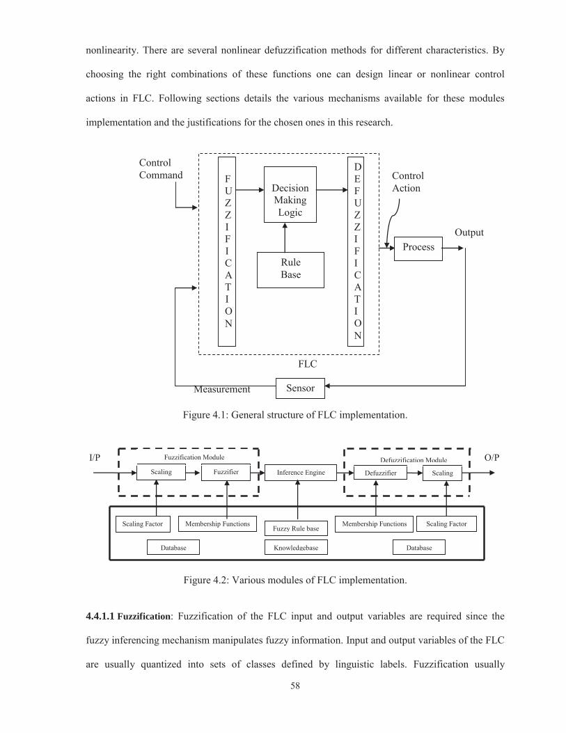
Figure 4.1 shows a general closed loop FLC implementation block diagram. Figure 4.2

shows various modules required for FLC implementation. As seen in Figure 4.2 FLC

implementation essentially requires fuzzification, defuzzification, rule base and inferencing

modules. The nature and number of these variables decides the resulting nonlinearity in a FLC. The

position, shape and number of membership functions on the premise side, as well as nonlinear input

scaling causes nonlinear characteristics. Even the rules themselves can express a nonlinear control

strategy. The inference engine making use of AND and OR connectives can also lead to

58

nonlinearity. There are several nonlinear defuzzification methods for different characteristics. By

choosing the right combinations of these functions one can design linear or nonlinear control

actions in FLC. Following sections details the various mechanisms available for these modules

implementation and the justifications for the chosen ones in this research.

Figure 4.1: General structure of FLC implementation.

Figure 4.2: Various modules of FLC implementation.

4.4.1.1 Fuzzification: Fuzzification of the FLC input and output variables are required since the

fuzzy inferencing mechanism manipulates fuzzy information. Input and output variables of the FLC

are usually quantized into sets of classes defined by linguistic labels. Fuzzification usually

F U Z Z I F I C A T I O N

D E F U Z Z I F I C A T I O N

Decision Making Logic

Rule Base

Process

Sensor

FLC

Measurement

Control Action

Output

Control Command

Fuzzifier Scaling Scaling Defuzzifier Inference Engine

Knowledgebase Database Database

Fuzzy Rule base Membership Functions Scaling Factor Membership Functions Scaling Factor

Fuzzification Module Defuzzification Module I/P O/P

59

transforms crisp normalized input data into membership grade of fuzzy sets defined on the

normalized Universe Of Discourse (UOD) of fuzzy variables and viewed as a generalization of the

concept of an ordinary set. So, fuzzification essentially means reading the grade of membership of

the crisp input value against the fuzzy set. However, since there can be overlap between two or

more fuzzy sets, so a crisp data might yield two or more membership grades. The input fuzzy sets

need to be so many in number and so positioned that (i) they cover the entire normalized UOD so

that any value of input variable will produce at least one nonzero membership value (as otherwise

no rule will be invoked form the control rule base), (ii) any two adjacent membership functions

overlap once and to such an extent that only two nonzero membership values are yielded by

fuzzification of each input variable.

The membership functions used in fuzzification process play a crucial role in the final

performance of an FLC. The choice of the membership function has a strong influence on the

control effect [Sun & Lin, 2002; Bagis, 2003]. Four types of membership functions are normally

used in most circumstances in control: Trapezoidal, Triangular [a case of trapezoidal], Gaussian

and Bell-shaped. Among these four, the first two are widely used. All these fuzzy sets are

continuous, normal and convex. A fuzzy set is said to be normal if its height is one. A fuzzy set is

said to be continuous if its membership function is continuous. The convexity property of fuzzy sets

is viewed as a generalization of the classical concepts of crisp sets. The number of fuzzy sets may

differ problem to problem under consideration. A large number of fuzzy variables give precise

modeling but introduce computational delay complexities. So, one need to have a tradeoff for the

timing aspect considering the number of input and output variables and number of resulting rules.

Membership functions characterize the fuzziness in fuzzy sets. However, the shape of the

membership functions, used to describe the fuzziness, has very few restrictions indeed. It might be

claimed that the rules used to describe the fuzziness are also fuzzy. Just as there are an infinite

number of ways to characterize fuzziness, there are infinite numbers of ways to graphically depict

the membership functions that describe fuzziness. Although the selection of membership function is

60

subjective, it cannot be arbitrary; it should be plausible.

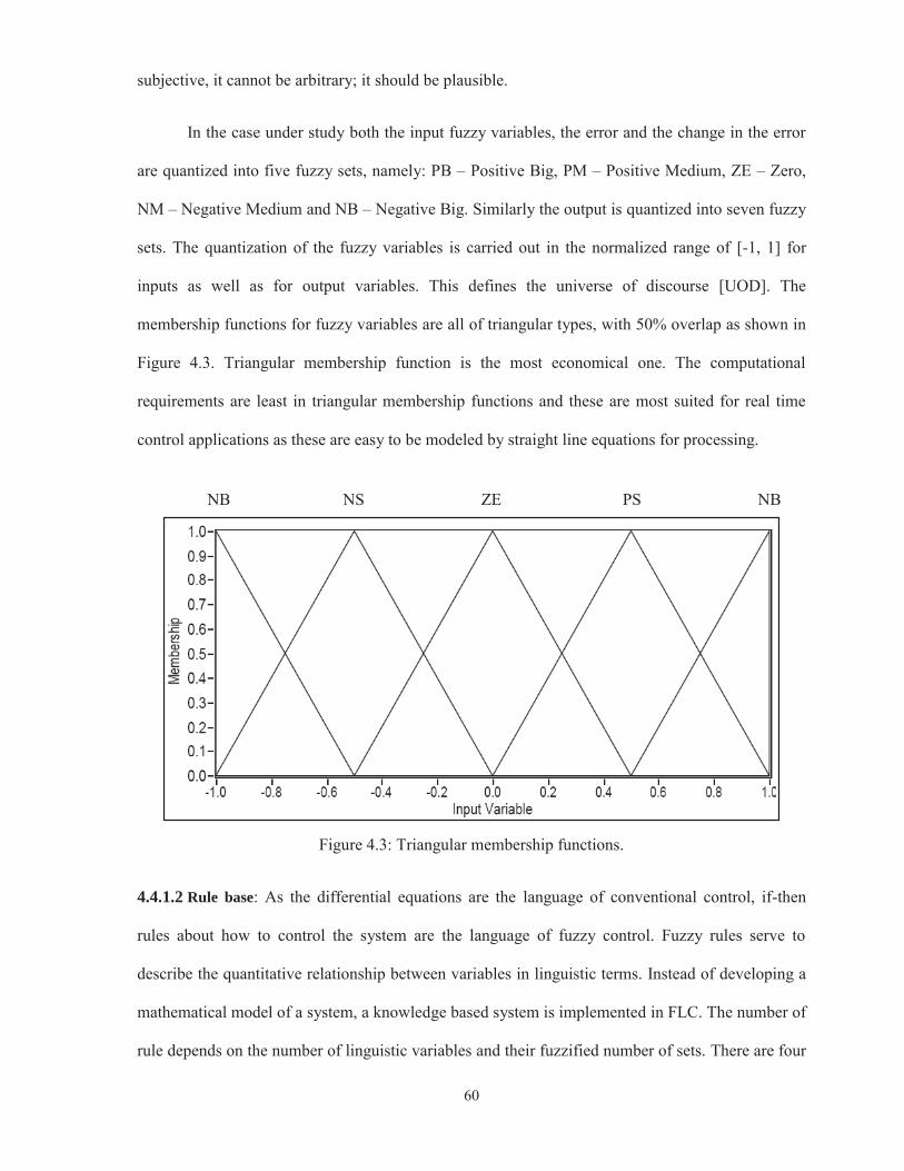
In the case under study both the input fuzzy variables, the error and the change in the error

are quantized into five fuzzy sets, namely: PB – Positive Big, PM – Positive Medium, ZE – Zero,

NM – Negative Medium and NB – Negative Big. Similarly the output is quantized into seven fuzzy

sets. The quantization of the fuzzy variables is carried out in the normalized range of [-1, 1] for

inputs as well as for output variables. This defines the universe of discourse [UOD]. The

membership functions for fuzzy variables are all of triangular types, with 50% overlap as shown in

Figure 4.3. Triangular membership function is the most economical one. The computational

requirements are least in triangular membership functions and these are most suited for real time

control applications as these are easy to be modeled by straight line equations for processing.

Figure 4.3: Triangular membership functions.

4.4.1.2 Rule base: As the differential equations are the language of conventional control, if-then

rules about how to control the system are the language of fuzzy control. Fuzzy rules serve to

describe the quantitative relationship between variables in linguistic terms. Instead of developing a

mathematical model of a system, a knowledge based system is implemented in FLC. The number of

rule depends on the number of linguistic variables and their fuzzified number of sets. There are four

NB NS ZE PS NB

61

principle methods used for rule base generation, (i) control engineering knowledge, (2) modeling

the operator behavior, (iii) fuzzy modeling, and (iv) self learning fuzzy controller. The first two

approaches are considered as heuristic methods while the other two are deterministic methods. The

heuristic method was used by Mamdani and the deterministic method by Tagaki and Sugeno.

For two input fuzzy variables, as the case under study, the rule base for FLC can be

imagined to be a two dimensional matrix. The rows represent the various linguistic values that a

variable can have and columns indicate the various values of another variable. The entries in this

matrix are the control action that has to be taken is described in the linguistic terms. The control

action is calculated based upon the experimentally observed process reaction [Lee, 1990a; Lee,

1990b]. The antecedent pairs in the rule structure are connected by a logical ‘AND’ operation

which is considered here as algebraic product triangular norm. It is chosen as it takes into account

the effect of all the inputs in comparison to the other methods of inference. It may be noticed that

the resulting control rules are non-linear as the output fuzzy sets are not linearly related to the input

fuzzy sets.

For the case under consideration, two input fuzzy variables of five membership functions

each and similarly seven membership functions for output variable. The rule base matrix will have

5x5 = 25 entries, considering all the possible combinations of inputs. It leads to 25 numbers of the

rules. Furthermore, each input variable will have two linguistic terms associated for each value of

the normalized input and there are two input variables leading to four adjacent rules getting fired in

every combination. Firing of four adjacent rules leads to total 16 formulas for FLC implementation.

4.4.1.3 Fuzzy inference mechanism: The basic function of the fuzzy inference engine is to compute

the overall value of the control output variable based on the individual contribution of each rule in

the rule base. In a fuzzy inference engine, the control actions are encoded by means of fuzzy

inference rules. The approximate fuzzy sets are defined on the domains of involved variables, and

fuzzy logic operators and inference methods are formalized in computational terms. The inference

62

method for FLC can be categorized into two groups direct and indirect. The direct inferencing

determines directly the output from the knowledge base and on line data by min-max operation.

The firing of a set of rules via the operation composition is called composition based inference. In

this case, the Fuzzy Relations [FRs] representing the meanings of each individual fuzzy rule are

aggregated into one FR describing the meaning of overall sets of fuzzy rules. Direct method is

normally used in FLC design as it is simple and offers use of min(t-norm)–max(t-conorm) operator.

This operator is called Mamdani type inference. For the present research work, Mamdani minimum

inference mechanism and product t-norms have been used. The differences in using the various

implication techniques are described in [Smith & Shen, 1998].

4.4.1.4 Defuzzification: This module converts the set of modified controller output value into a

single crisp value. This is required as the actuator cannot operate upon the fuzzy commands, rather

requires crisp inputs for their operation. There are many procedures outlined in the literature

[Thomas, 1997] for defuzzification which are centre of gravity/area, centre of mass, centre of

largest area, first of maxima, middle of maxima, and height. Of these, the Centre Of Gravity (COG)

as shown in Eq. [4.1] is the most efficient for the fact that it gives a defuzzified output which

conveys the real meaning of the action that has to be taken at that instant. Here is the

membership grade and x is the fuzzy variable. In the present work, the center of gravity

defuzzification method is used to defuzzify composite fuzzy controller output into a crisp control

signal [Tang, Man, Chen & Kwong, 2001].

x* = [4.1]

4.4.1.5 FLC tuning: The tuning of a fuzzy controller is often compared to the tuning of a PID,

stressing the large number of the fuzzy controller parameters, compared to the three gains of a PID.

In the experiment conducted the tuning was done manually by optimizing the close loop step

response for minimum overshoot and faster response at some sample frequencies [Li, 1997; Preitl,

1999].

63

4.4.2 Fuzzy PI controller structure

A conventional PI controller follows the following control low:

(t) = [e(t) + (t)dt] [4.2]

where is the proportional constant of PI controller, I is the integral time constant, e(t) is error

in the acceleration waveform amplitude, e(t) = r(t) – y(t), r(t) is the desired acceleration amplitude,

y(t) is the output obtained from the shaker process and (t) is the output of the PI controller. On

differentiating Eq. [4.1] and putting into a discrete form,

: ; = >

: ; + s

τ e(t)]

In a discrete form, for a given sampling period Ts, the above equation can be written as: > ?F > Fs ? = >

> ?F > Fs? + s

τ e[k]],

or, Δ [k] = >Δe[k] + τ

e[k]],

or, ΔuPI[k] = KCΔe[k] + K’Ce[k] [4.3]

where, ΔuPI[k] = > ?F > F s?

and, Δe[k] = e > ?F > F s?

KC is defined as the gain P

and, K’C = KC τ is the gain I.

The denormalized output of fuzzy controller is given by Δ [k], where, gain KUPI

denormalizes the normalized incremental fuzzy controller output, Δ [k]. The controlled output is

thus obtained as,

[k] = [k-1] + [k] [4.4]

In this work the control action is implemented on the acceleration waveform basis and

hence the amplitude of the excitation signal to the power amplifier is controlled to achieve the

desired objective. To implement the proposed acceleration waveform amplitude fuzzy PI controller

64

Eq. [4.2], two inputs namely the instantaneous acceleration waveform amplitude error e[k] and its

change of the error Δe[k] are required and the output of the FLC is the incremental change in the

controller output of excitation waveform to be fed to the power amplifier. Increasing the number of

inputs to FLC would require more processing time for the larger rule base size and hence would

force a constraint on the implementable update rate in acceleration amplitude control. Small

computational delays also enable the shaker control at high frequencies. In order to make the

computations faster a customized fuzzy PI controller was chosen rather than other combinations

such as fuzzy PI + fuzzy PD or fuzzy PID itself [Carvajal, Chen & Ogmen, 2000]. A physical

meaning of the parameters for the fuzzy PI controller remains the same like that for the classical PI

controller. The controller takes two fuzzy variable e[k] and Δe[k] and it gives an incremental

control action ΔuPI.

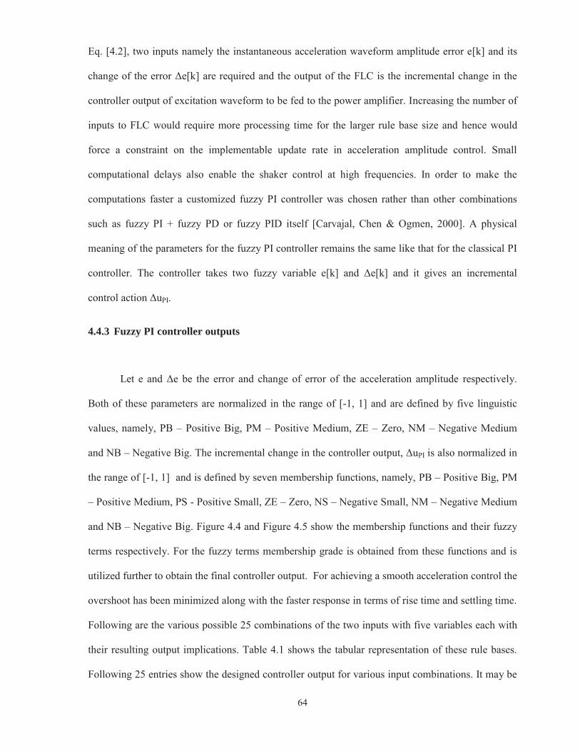
4.4.3 Fuzzy PI controller outputs

Let e and Δe be the error and change of error of the acceleration amplitude respectively.

Both of these parameters are normalized in the range of [-1, 1] and are defined by five linguistic

values, namely, PB – Positive Big, PM – Positive Medium, ZE – Zero, NM – Negative Medium

and NB – Negative Big. The incremental change in the controller output, ΔuPI is also normalized in

the range of [-1, 1] and is defined by seven membership functions, namely, PB – Positive Big, PM

– Positive Medium, PS - Positive Small, ZE – Zero, NS – Negative Small, NM – Negative Medium

and NB – Negative Big. Figure 4.4 and Figure 4.5 show the membership functions and their fuzzy

terms respectively. For the fuzzy terms membership grade is obtained from these functions and is

utilized further to obtain the final controller output. For achieving a smooth acceleration control the

overshoot has been minimized along with the faster response in terms of rise time and settling time.

Following are the various possible 25 combinations of the two inputs with five variables each with

their resulting output implications. Table 4.1 shows the tabular representation of these rule bases.

Following 25 entries show the designed controller output for various input combinations. It may be

65

noted that the resulting controller output is in the incremental from.

Figure 4.4: I/P membership functions.

Figure 4.5: O/P membership functions.

-2x+2

0.0

1.0

μ

-2x

NL NS ZE PS PL

-1.0 -0.5 0.0 0.5 1.0

-2x-1 -2x+1

2x+2 2x+1 2x 2x-1

μ

NL NM NS ZE PS PM PL

-1.0 -0.67 -0.33 0.0 0.33 0.67 1.0

-3x+3-3x-1 -3x -3x+1 -3x+2-3x-2

3x-1 3x+2 3x+1 3x 3x-2 3x+3

0.0

1.0

66

Table 4.1: Rule Base for Fuzzy PI Controller Change of error (Δe)

error(e)

NB NM ZE PM PB

NB NL NM NM NS ZE

NM NM NS NS ZE PS

ZE NM NS ZE PS PM

PM NS ZE PS PS PM

PB ZE PS PM PM PL

13. e = ZE. AND. Δe = ZE → ΔuPI = ZE3

14. e = ZE. AND. Δe = PS → ΔuPI = PS2

15. e = ZE. AND. Δe = PL → ΔuPI = PM1

16. e = PS. AND. Δe = NL → ΔuPI = NS5

17. e = PS. AND. Δe = NS → ΔuPI = ZE4

18. e = PS. AND. Δe = ZE → ΔuPI = PS3

19. e = PS. AND. Δe = PS → ΔuPI = PS4

20. e = PS. AND. Δe = PL → ΔuPI = PM2

21. e = PL. AND. Δe = NL → ΔuPI = ZE5

22. e = PL. AND. Δe = NS → ΔuPI = PS5

23. e = PL. AND. Δe = ZE → ΔuPI = PM3

24. e = PL. AND. Δe = PS → ΔuPI = PM4

25. e = PL. AND. Δe = PL → ΔuPI = PL

1. e = NL. AND. Δe = NL → ΔuPI = NL

2. e = NL. AND. Δe = NS → ΔuPI = NM1

3. e = NL. AND. Δe = ZE → ΔuPI = NM2

4. e = NL. AND. Δe = PS → ΔuPI = NS1

5. e = NL. AND. Δe = PL → ΔuPI = ZE1

6. e = NS. AND. Δe = NL → ΔuPI = NM3

7. e = NS. AND. Δe = NS → ΔuPI = NS2

8. e = NS. AND. Δe = ZE → ΔuPI = NS3

9. e = NS. AND. Δe = PS → ΔuPI = ZE2

10. e = NS. AND. Δe = PL → ΔuPI = PS1

11. e = ZE. AND. Δe = NL → ΔuPI = NM4

12. e = ZE. AND. Δe = NS → ΔuPI = NS4

67

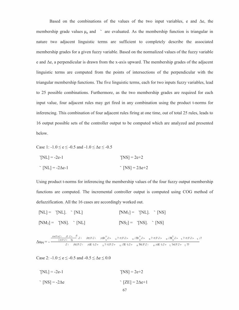
Based on the combinations of the values of the two input variables, e and Δe, the

membership grade values and ` are evaluated. As the membership function is triangular in

nature two adjacent linguistic terms are sufficient to completely describe the associated

membership grades for a given fuzzy variable. Based on the normalized values of the fuzzy variable

e and Δe, a perpendicular is drawn from the x-axis upward. The membership grades of the adjacent

linguistic terms are computed from the points of intersections of the perpendicular with the

triangular membership functions. The five linguistic terms, each for two inputs fuzzy variables, lead

to 25 possible combinations. Furthermore, as the two membership grades are required for each

input value, four adjacent rules may get fired in any combination using the product t-norms for

inferencing. This combination of four adjacent rules firing at one time, out of total 25 rules, leads to

16 output possible sets of the controller output to be computed which are analyzed and presented

below.

Case 1: -1.0 ≤ e ≤ -0.5 and -1.0 ≤ Δe ≤ -0.5

[̀NL] = -2e-1 [̀NS] = 2e+2

` [NL] = -2Δe-1 ` [NS] = 2Δe+2

Using product t-norms for inferencing the membership values of the four fuzzy output membership

functions are computed. The incremental controller output is computed using COG method of

defuzzification. All the 16 cases are accordingly worked out.

[̀NL] = [̀NL]. ` [NL] [̀NM1] = [̀NL]. ` [NS]

[̀NM3] = [̀NS]. ` [NL] [̀NS2] = [̀NS]. ` [NS]

ΔuPI = - swFxJ: ;F J> ?t

{ctFJ> ?gJ: ;ktFJ: ;oE

v

uJ> u?:tFJ> u;?E

v

uJ> s?:tFJ> s;?E

t

uJ> t?:tFJ> t;?

J: ;ktFJ: ;oE tJ> u?:tFJ> u;?E tJ> s?ktFJ: s;oE tJ> t?>tFJ> t??

Case 2: -1.0 ≤ e ≤ -0.5 and -0.5 ≤ Δe ≤ 0.0

[̀NL] = -2e-1 [̀NS] = 2e+2

` [NS] = -2Δe ` [ZE] = 2Δe+1

68

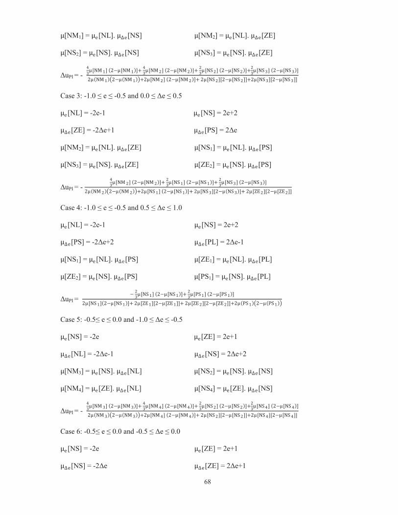
[NM1] = [NL]. [NS] [NM2] = [NL]. [ZE]

[NS2] = [NS]. [NS] [NS3] = [NS]. [ZE]

ΔuPI = -

Case 3: -1.0 ≤ e ≤ -0.5 and 0.0 ≤ Δe ≤ 0.5

[NL] = -2e-1 [NS] = 2e+2

[ZE] = -2Δe+1 [PS] = 2Δe

[NM2] = [NL]. [ZE] [NS1] = [NL]. [PS]

[NS3] = [NS]. [ZE] [ZE2] = [NS]. [PS]

ΔuPI = -

Case 4: -1.0 ≤ e ≤ -0.5 and 0.5 ≤ Δe ≤ 1.0

[NL] = -2e-1 [NS] = 2e+2

[PS] = -2Δe+2 [PL] = 2Δe-1

[NS1] = [NL]. [PS] [ZE1] = [NL]. [PL]

[ZE2] = [NS]. [PS] [PS1] = [NS]. [PL]

ΔuPI =

Case 5: -0.5≤ e ≤ 0.0 and -1.0 ≤ Δe ≤ -0.5

[NS] = -2e [ZE] = 2e+1

[NL] = -2Δe-1 [NS] = 2Δe+2

[NM3] = [NS]. [NL] [NS2] = [NS]. [NS]

[NM4] = [ZE]. [NL] [NS4] = [ZE]. [NS]

ΔuPI = -

Case 6: -0.5≤ e ≤ 0.0 and -0.5 ≤ Δe ≤ 0.0

[NS] = -2e [ZE] = 2e+1

[NS] = -2Δe [ZE] = 2Δe+1

69

[NS2] = [NS]. [NS] [NS3] = [NS]. [ZE]

[NS4] = [ZE]. [NS] [ZE3] = [ZE]. [ZE]

ΔuPI = -

Case 7: -0.5≤ e ≤ 0.0 and 0.0 ≤ Δe ≤ 0.5

[NS] = -2e [ZE] = 2e+1

[ZE] = -2Δe+1 [PS] = 2Δe

[NS3] = [NS] . [ZE] [ZE2] = [NS]. [PS]

[ZE3] = [ZE]. [ZE] [PS2] = [ZE]. [PS]

ΔuPI =

Case 8: -0.5≤ e ≤ 0.0 and 0.5 ≤ Δe ≤ 1.0

[NS] = -2e [ZE] = 2e+1

[PS] = -2Δe+2 [PL] = 2Δe-1

[ZE2] = [NS]. [PS] [PS1] = [NS]. [PL]

[PS2] = [ZE]. [PS] [PM1] = [ZE]. [PL]

ΔuPI =

Case 9: 0.0≤ e ≤ 0.5 and -1.0≤ Δe ≤ -0.5

[ZE] = -2e+1 [PS] = 2e

[NS] = 2Δe+2 [NL] = -2Δe-1

[NM4] = [ZE]. [NL] [NS4] = [ZE]. [NS]

[NS5] = [PS]. [NL] [ZE4] = [PS]. [NS]

ΔuPI = -

Case 10: 0.0≤ e ≤ 0.5 and -0.5≤ Δe ≤ 0.0

[ZE] = -2e+1 [PS] = 2e

[NS] = -2Δe [ZE] = 2Δe+1

70

[NS4] = [ZE]. [NS] [ZE3] = [ZE]. [ZE]

[ZE4] = [PS]. [NS] [PS3] = [PS]. [ZE]

ΔuPI =

Case 11: 0.0≤ e ≤ 0.5 and 0.0≤ Δe ≤ 0.5

[ZE] = -2e+1 [PS] = 2e

[ZE] = -2Δe+1 [PS] = 2Δe

[ZE3] = [ZE]. [ZE] [PS2] = [ZE]. [PS]

[PS3] = [PS]. [ZE] [PS4] = [PS]. [PS]

ΔuPI =

Case 12: 0.0≤ e ≤ 0.5 and 0.5≤ Δe ≤ 1.0

[ZE] = -2e+1 [PS] = 2e

[PS] = -2Δe+2 [PL] = 2Δe-1

[PS2] = [ZE]. [PS] [PM1] = [ZE]. [PL]

[PS4] = [PS]. [PS] [PM2] = [PS]. [PL]

ΔuPI =

Case 13: 0.5≤ e ≤ 1.0 and -1.0≤ Δe ≤ -0.5

[PS] = -2e+2 [PL] = 2e-1

[NL] = -2Δe-1 [NS] = 2Δe+2

[NS5] = [PS]. [NL] [ZE4] = [PS]. [NS]

[ZE5] = [PL]. [NL] [PS5] = [PL]. [NS]

ΔuPI =

71

Case 14: 0.5≤ e ≤ 1.0 and -0.5≤ Δe ≤ 0.0

[PS] = -2e+2 [PL] = 2e-1

[NS] = -2Δe [ZE] = 2Δe+1

[ZE4] = [PS]. [NS] [PS3] = [PS]. [ZE]

[PS5] = [PL]. [NS] [PM3] = [PL]. [ZE]

ΔuPI =

Case 15: 0.5≤ e ≤ 1.0 and 0.0≤ Δe ≤ 0.5

[PS] = -2e+2 [PL] = 2e-1

[ZE] = -2Δe+1 [PS] = 2Δe

[PS3] = [PS]. [ZE] [PS4] = [PS]. [PS]

[PM3] = [PL]. [ZE] [PM4] = [PL]. [PS]

ΔuPI =

Case 16: 0.5≤ e ≤ 1.0 and 0.5≤ Δe ≤ 1.0

[PS] = -2e+2 [PL] = 2e-1

[PS] = -2Δe+2 [PL] = 2Δe-1

[PS4] = [PS]. [PS] [PM2] = [PS]. [PL]

[PM4] = [PL]. [PS] [PL] = [PL]. [PL]

ΔuPI =

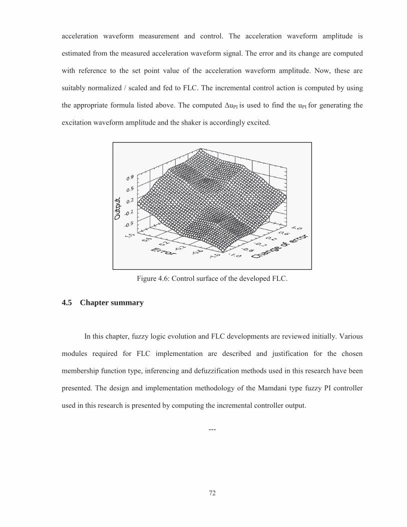
To observe the nature of available control actions, in the entire UOD, a three dimensional

plot is generated by varying the two FLC inputs and recording the incremental FLC output. Figure

4.6 shows the resulting fuzzy control surface. As seen clearly, it forms a non-linear control action.

For implementing this controller in real time a LabVIEW code is developed for the formulas

worked out as above and integrated with the Data Acquisition (DAQ) module of the software for

72

acceleration waveform measurement and control. The acceleration waveform amplitude is

estimated from the measured acceleration waveform signal. The error and its change are computed

with reference to the set point value of the acceleration waveform amplitude. Now, these are

suitably normalized / scaled and fed to FLC. The incremental control action is computed by using

the appropriate formula listed above. The computed ΔuPI is used to find the uPI for generating the

excitation waveform amplitude and the shaker is accordingly excited.

Figure 4.6: Control surface of the developed FLC.

4.5 Chapter summary

In this chapter, fuzzy logic evolution and FLC developments are reviewed initially. Various

modules required for FLC implementation are described and justification for the chosen

membership function type, inferencing and defuzzification methods used in this research have been

presented. The design and implementation methodology of the Mamdani type fuzzy PI controller

used in this research is presented by computing the incremental controller output.

---

SECTION - I

Complex Vibrations Measurement and Presentation