fuzzy technology application for mobile positioning...
TRANSCRIPT

FUZZY TECHNOLOGY APPLICATION FOR MOBILE POSITIONING IN CELLULAR COMMUNICATION
Aleksandar Stojcevski B.E. (Electrical/Electronic)
A thesis submitted in fulfillment of the requirements for the degree of
Master of Engineering
VICTORIA I UNIVERSITY
H m « X
z O r-
o
School of Communications & Informatics
Faculty of Engineering and Science
Victoria University of Technology
Melbourne, Australia
September 2000

2 £QC=>£ 7 &
rFTS THESIS 621.38456 STO 30001006983276 ^tnicevski, Aleksandar Fuzzy Technology application for mobile positioning in cellular communication

Declaration
I declare that, to the best of m y knowledge, the research described herein is the result of
m y own work, except where otherwise stated in the text. It is submitted in fulfillment of
the candidature for the degree of Masters by Research in Engineering at Victoria
University, Australia. N o part of this work has already been submitted for any degree nor
is being submitted for any other degree.
Aleksandar Stojcevski
September 2000

ABSTRACT
In engineering systems there is generally two classes of knowledge: objective knowledge,
which can be quantified using the laws of traditional mathematics, and subjective or
intelligent knowledge, that cannot be modeled mathematically but can be expressed in
linguistical terms. Fuzzy Logic (FL) is a method that combines these two forms of
knowledge, and as such provides a powerful tool for solving real engineering problems.
A fuzzy logic system (FLS) is the methodology of applying FL to engineering systems.
In general, a FLS can be considered as a non-linear mapping of crisp (firm) input data to
crisp output data. It is the inclusion of subjective knowledge in a FLS that leads to a
plethora of mapping possibilities, which may not be possible using traditional
mathematical modeling techniques. A fuzzy logic system consists of four main elements:
fuzzification, rule based, inference engine and deffuzification.
Fuzzy logic has been successfully adopted in many real-world automatic control systems
including automobile transmission, subway systems, industrial robots, washing machines,
cameras and air-conditioners. In contrast, the utilization of fuzzy logic in mobile
communications systems is recent and limited. Understanding general mobile
communications is essential in order to go on and develop a mobile positioning
application.
The successful applications of Fuzzy Logic Control (FLC) techniques in many areas draw
a huge amount of attention to its industrial applications. However, lack of structured
methods and tools for design and analysis is preventing this revolutionary controller from
playing a more significant role in mobile communications.
A methodology to construct and analyse a FL controller to be used in mobile positioning
would significantly improve the efficiency of F L C design, increase the quality of F L C by
allowing the designer to develop and design the controller based on some specifications
and requirements, and then validate that design.

/ dedicate my work to my father
RADE STOJCEVSKI
His endless support and encouragement has been a great
inspiration for the completion of this work.

TABLE OF CONTENTS
ACKNOWLEDGMENTS i
LIST OF ABBREVIATIONS ii
LIST OF FIGURES vi
LIST OF TABLES viii
CHAPTER 1: INTRODUCTION THEORY
1.1 Introduction 1
1.2 Existing Communication Technologies 1
1.3 Mobile Location System 3
1.4 Project Formulation 10
1.4.1 Objectives of the Work 10
1.4.2 Methodologies and Techniques 11
1.4.3 Thesis Breakdown 11
CHAPTER 2: THEORETICAL INTRODUCTION AND LITERATURE REVIEW
2.1 Introduction 13
2.2 Analysis of Handover Algorithms 13
2.3 Signal Strength Model . 14
2.4 Analysis of Positioning Algorithm 16
2.5 Mobile Positioning Distribution 18
2.6 Fuzzy Logic 18
CHAPTER 3: EXSISTING POSITIONING MODELS
3.1 Introduction 26
3.2 Ericssons' Model 26
3.3 Cambridge Positioning Systems Limited 27

CHAPTER 4: ERICSSONS' POSITIONING MEASUREMENT SYSTEM
4.1 Introduction 31
4.2 Positioning Simulator 31
4.2.1 System Simulator 33
4.2.1.1 Structure of the System Simulator 33
4.2.1.2 System Simulator Parameters 35
4.2.1.3 Output from the System Simulator 37
4.2.2 Radio Link Simulator 38
4.2.3 Channel Model 39
CHAPTER 5: PROPOSED CHANNEL MODEL
5.1 Introduction 40
5.2 Modeling Parameters 40
5.2.1 Delay Spread 40
5.2.2 Correlation of Delay Spread Measurements at Different Base Stations 42
5.2.3 Power Delay Profile Shapes 42
5.2.4 Fading and Angles of Arrival 43
5.3 Channel Model Based on the CODIT Model 44
5.4 Matching the Delay Spread of the Channel Model to the Delay Spread Model 46
5.5 Unresolved Issues 47
5.6 Definition of the Environments 48
5.7 Base Station Antenna Diversity 49
5.8 G S M Adaptation 51
5.8.1 FIR Filter Implementation 51
5.8.2 Sampling in Time Domain 53
5.8.3 Frequency Hopping 54
5.9 Additional Explanation on the Channel Model 54
5.9.1 Antenna Space Diversity 54
5.9.2 Number of Scaterers 57
5.9.3 Scaling of the Time Axis 59

5.9.4 Range of Validity 59
5.9.5 Delay Spread vs. Distance-Some Physical Reasons 59
5.10 Matlab Software Package 61
CHAPTER 6: POSITIONING METHODS
6.1 Introduction 64
6.2 The Up-Link T O A Method 64
6.2.1 T O A Estimation 66
6.2.1.1 The Estimation Problem 66
6.2.1.2 Channel Estimation Algorithm 67
6.2.1.3 Multipath Rejection (ICI-MPR) 68
6.2.2 T O A Simulation Chain 70
6.3 The Enhanced-Observed Time Difference (E-OTD) Method 72
6.3.1 M S Based Location System 72
6.3.2 Benefits and Applications 73
6.3.3 E-OTD Computations 74
6.3.3.1 Cramer-Rao Bound 75
CHAPTER 7: POSITION CALCULATION AND STATISTICAL EVALUATION
7.1 Introduction 77
7.2 "Average Algorithm" Positioning Method 78
7.3 "More Preferable Solution" Positioning Method 86
CHAPTER 8: FUZZY LOGIC POSITIONING
8.1 Introduction 92
8.2 Enhanced Fuzzy Positioning Method 97

CHAPTER 9: COMPARISONS AND CONCLUSIONS
9.1 Introduction 103
9.2 Techniques and Results Comparison 103
9.3 Conclusions 105
9.4 Future Work 105
REFERENCES 107
APPENDIX A: System Simulator Matlab files 114
APPENDIX B: Channel Model Matlab files 117
APPENDIX C: System Simulator based on Statistical files (Matlab file) 124
A P P E N D I X D: Matlab file estimating mobile position 126

ACKNOWLEDGMENTS
I a m indebted to many people for advice and assistance. First on m y list, m y supervisors
Dr. Leonid Reznik and Professor Mike Faulkner. Their support and wisdom will never
be forgotten. Thanks also to Dr. Jugdutt Singh, Mr. Ranjan Mohapatra, research assistant
Melvyn Parrera, and the Mobile Communications & Signal Processing Group at Victoria
University for their help.
A special thanks for encorangment goes out to my great friend Mr. Dean Cvetkovic.
Thanks also to the Stojcevski family, m y father Mr. Rade Stojcevski, Mrs. Vera
Stojcevska, Bobby Stojcevski and Filip Stojcevski, for their support, patience and
understanding.
Aleksandar Stojcevski
i

LIST OF ABBRIVIATIONS
F D M A Frequency Division Multiple Access
T D M A Time Division Multiple Access
C D M A Code Division Multiple Access
G S M Global System Mobile
M P S Mobile Positioning System
T O A Time of Arrival
A O A Angle of Arrival
T D O A Time Difference of Arrival
RF Radio Frequency
GPS Global Positioning System
a Estimated angle of incidence of the propagation wave
c Speed of Light
At Difference between the time of arrival signals
X Radio signal wavelength
<j> Arriving electrical phase angle
p,sec Micro seconds
m Meters
FCC Federal Communication Commission
E911 Emergency nine one one
F M Frequency Modulation
A M Amplitude Modulation
km Kilometres
FL Fuzzy Logic
FLC Fuzzy Logic Control
DSP Digital Signal Processing
S N R Signal to Noise Ratio
s(t) Received Signal Power
m(t) Local Mean of the Received Signal
ii

r(t) Fast Fading Component
A(n) Discrete Time Signal
a Standard Deviation
v Velocity of Mobile
T Sampling Interval
RA(k) Autocorrelation
t Path Delay
L Distance between Base Station and Mobile Station
BS Base Station
M S Mobile Station
X m X coordinate of Mobile
Y m Y coordinate of Mobile
XBs X coordinate of Base Station
Y B S Y coordinate of Base Station
A V L Automatic Vehicle Location
D Distance between Base Stations
SR Rhomboid
C O G Centre of Gravity
F M Fuzzy Mean
W F M Weighted Fuzzy Mean
F A A H Fuzzy Adaptive-interval and Hysterisis threshold handover
A V G Averaging Interval
H Y S Hysterisis Level
K 2 Propagation Constant
d0 Correlation Distance
Ki Transmitter Power
apdp Average Power Delay Profile
CPS Cambridge Positioning Systems
R M S Root Mean Square
P(x,y) Circular Distribution
B C C H Broadcast Control Channel
iii

Pt Transmitted Power
G a Antenna Gain
Gf Lognormal Fading
C/I Carrier to Interference Ratio
M A T L A B Computing environment for high performance numerical computing and
Visualisation
C/N Carrier to Noise Ratio
rmse Root Mean Square Error
x Delay Spread
T w Excess Time Delay
Oi Mean Angle of Arrival at Mobile
LOS Line of Sight
Tm Mean Delay
9j Angle of Arrival
Hz Hertz
p.s Micro Seconds
N L O S Non Line of Sight
E-OTD Enhanced-Observed Time Difference
M L C Mobile Location Centre
D T C D Digital Channel Designation
N snapshots
a„ Amplitude of Incoming Waves
Tn Delay of Incoming Waves
m Nakagami Parameters
CIR Channel Impulse Response
CPP Channel Power Profile
ICI Incoherent Integration
Eb/N0 Bit Energy to Noise Power Spectral Density
R T D Real Time Difference
BTS Base Transceiver Station
O T D Observed Time Difference
iv

C D F Cumulative Distribution Function
bsv Array containing Base Station coordinates
t Time of Arrival (seconds)
T Bit Energy to Noise Power Ratio
Wi Weighted Average
Wsi Belief Degree based on Signal Strength
W n Belief Degree based on Bit Energy to Noise Power
V

LIST OF FIGURES
Figure 1.1: Location determination by angle of arrival (AOA)
Figure 1.2: Location determination by time distance of arrival (TDOA)
Figure 2.1: Arrival times of pilot tones to the Mobiles
Figure 2.2: Position finding by use of hyperbolas
Figure 2.3: Area of possible mobile positions
Figure 2.4: Handover Process
Figure 2.5: Mobile communications with two base stations A and B
Figure 3.1: Circular Distribution
Figure 3.2: The observed and predicted, spread of measurements
Figure 3.3: Results from residential area
Figure 4.1: Positioning Simulator
Figure 4.2: System Simulator
Figure 4.3: Radio Link Simulator
Figure 5.1: The basics of the CODIT channel model
Figure 5.2: Generating the diffuse scatterers for the Hilly channel models of the
CODIT model
Figure 5.3: Model of the local scattering
Figure 5.4: Sample channel for evaluation of the base station angle of arrival model
Figure 5.5: Power azimuth spectrum using the model with uniform excess delay
distribution and equal scatterer power (bars), and for a Laplacian
distribution (continuous line). The x-axis is the azimuth angle [deg] and
on the y-axis the relative power
Figure 5.6: Phase shifts of waves due to their angle of arrival at the different base
station antennas
Figure 5.7: Plane wave impinging on two spatially separated antennas
Figure 5.8: Local scattering
Figure 6.1: GSM transmission chain with time of arrival estimation
Figure 6.2: Generic E-OTD signaling flow in MS based location calculation
VI

Figure 7.1: Three Base Stations & Original Mobile Station
Figure 7.2: Position estimates with BS1 & BS2 operating
Figure 7.3: Position estimates with BS1 & BS3 operating
Figure 7.4: Position estimates with BS2 and BS3 operating
Figure 7.5: Average estimated mobile position for a3BS system
Figure 7.6: Average estimated mobile position, for a 5 BS system
Figure 7.7: Average estimated mobile position, for a 7 BS system
Figure 7.8: Three base station system, Method 2, with BS3 deciding
Figure 7.9: BS1 & BS2 operating, while BS3 makes the decision, 3 BS system
Figure 7.10: BS1 & BS3 operating, while BS2 makes the decision, 3 BS system
Figure 7.11: BS2 & BS3 operating, while BS1 makes the decision, 3 BS system
Figure 7.12: Average position estimate, 5 BS system, using Method 2
Figure 7.13: Average position estimate, 7 BS system, using Method 2
Figure 8.1: Membership function chart.
Figure 8.2: Example of a fuzzy output curve.
Figure 8.3: Base station-Mobile station connections.
Figure 8.4: Average position estimate, 3 BS system, using fuzzy method.
Figure 8.5: Average position estimate, 5 BS system, using fuzzy method.
Figure 8.6: Average position estimate, 7 BS system, using fuzzy method.
VII

LIST OF TABLES
Table 2.1: Simulation Parameters
Table 4.1: General parameters to ihe system simulator
Table 4.2: Parameters dependent on environment
Table 5.1: Suggested parameter values for the Greenstein delay spread model
Table 5.2: Parameters for the CODIT channel model
Table 5.3: Terrain Definitions
Table 8.1: Linguistic meanings of fuzzy logic values.
Table 8.2: Membership function
Table 8.3: Fuzzy logic operations.
Table 8.4: Comparison of Boolean Logic and Fuzzy Logic Operations.
Table 9.1: Result summary for method 1.
Table 9.2: Result summary for method 2.
Table 9.3: Result summary for method 3.
viii

Introduction Theory
CHAPTER 1
INTRODUCTION THEORY
1.1 Introduction
Reliable communications is a virtual component for improvement in performance and
increased functionality in mobile location. It provides a very valuable opportunity to
present relevant information to the mobile and its occupants. Many quality services can
be provided to mobiles using communications technologies.
Communications technologies are poised for major expansion in two key areas: wireless
data communications and high-speed wireless (wire-based) communications supported by
the Internet and ancillary networks. Ultimately it will be the marriage of these two key
technologies that will bring about a revolution resulting in a new information society.
Wireless data applications play a critical role in making the vision of mobile computing a
reality. Today's competitive and fast-placed business climate demands tools that allow
people to communicate at their o w n convenience and discretion.
1.2 Existing communications technologies
Mobile communications networks need to support many different applications within a
wide set of user services including traffic management, emergency management,
electronic payment and last but not least mobile location. Each application has specific
needs that may best be satisfied by a particular communications technology. Because no
single communications technology can satisfy all of these requirements, a hybrid
implementation of technologies is likely to be required for a regional or statewide
communications network.
Both analog and digital systems are available for mobile radios (the digital systems are
essentially related to voice digitisation and to digital transmissions). The major
advantages of the digital systems over the analog systems are increased spectrum
1

Introduction Theory
efficiency, more consistent audio quality throughout more of the coverage area, inherent
privacy from analog scanners, and greater data rate capability.
Some of the transmission and switching methods used for transmission of information is
briefly considered next. Three major channel access methods exist: F D M A (frequency-
division multiple access), T D M A (time-division multiple access), and C D M A (code-
division multiple access) [1]. F D M A and T D M A can be implemented on either
narrowband channels (e.g., 12.5 kHz) or wideband channels (e.g., 200 kHz), whereas
C D M A is restricted to the wideband architecture. T w o principal switching techniques
are available: circuit stitching and packet switching. Circuit switching requires the
complete end-to-end connection over both the wireless and wired segments before any
voice or data can be sent. Packet switching divides the information into packets and
transfers packets of data between network nodes over different connections until the
packets reach their final destination and are reconstructed for the user. The main
difference between these two methods is that circuit switching reserves the required
bandwidth in advance, whereas packet switching acquires and releases it on an as-needed
bias.
In general, mobile services can be classified into conventional (nontrunked) mobile
systems and trunked mobile systems. Each conventional mobile system has one channel
available for each specific group of users. In other words, users are grouped so that each
group of users is assigned to a different channel. This system is less efficient than
trunking because users can only communicate if their channel is free. Since each group
of users shares a c o m m o n radio frequency, the users end up competing for airtime. The
trunked mobile system allows all available channels to be shared among a large group of
users, so that no one is waiting as long as free channels are available. For instance, a
typical trunked land mobile radio system can have up to 28 channels, one of which is a
dedicated control channel that automatically assigns the open channels to users. W h e n a
user wants to transmit, both the transmitting radio and the receiving radios are
automatically assigned to one of the 28 available radio channels. This system is better at
conserving spectrum, since no individual radio user will have to wait to transmit if a
2

Introduction Theory
trunked radio channel is available. Depending on how the available spectrum is used,
these systems can also be classified as narrowband or wideband. In the narrow
architecture, the total frequency band is split into several narrowband channels. In the
wideband architecture, most of the spectrum is available to each and every user.
1.3 Mobile Location Systems
Mobile positioning has received a lot of attention recently. Applications are both of
commercial and public interest. Most papers published today illustrate the performance of
a mobile positioning technique applicable to the Global System Mobile ( G S M ) network.
The ability of a G S M network to locate a mobile station is reduced, for the time being, to
the facility required by the mobility management function, i.e. the cell identity. There are
some ways of improving a rough position of a mobile unit.
One of them for example is by using the timing advance information and the management
reports. The accuracy could be in the order of a few hundred meters. This figure is still
not accurate enough for the effective development of a number of new added value
services and emergency services.
Some of the general questions that arise among us today about mobile positioning are
questions such as: What does G S M based positioning do? What is the Mobile Positioning
System (MPS)? What are its applications? and what are the standards today? G S M based
positioning is used to geographically locate mobile phones and to distribute the
positioning information to different applications. All existing mobile phones can
potentially be positioned since no changes are needed in the phone itself. Mobile
positioning system (MPS) is the system used to find out and provide the geographical
position of a mobile phone to an application. A cellular positioning system is only using
the infrastructure and characteristics of the mobile telephony network to find out the
geographical location of a mobile unit. Positioning could be used in whole range of
applications. Examples of positioning applications are:
• Fleet management
• Tracking asset or goods
3

Introduction Theory
• Stolen vehicle recovery
• Emergency call positioning
• Local traffic and weather
information
• Directions to different closest
gas stations, etc.
Mobile location systems can be broadly categorised onto two classes: autonomous and
centralised. Whenever location functions are performed at the mobile end with no remote
host or centralised computing facilities involved, the system will be referred to as
autonomous system Otherwise, the system will be referred to as a cenralised system.
Good systems architecture is very important for successful location. Users' requests and
developers' improvements generally lead to system expansion. A good architecture must
provide a stable base for the future evolution of the system. In other words, the systems
must be stable and predictable, but still flexible enough to meet changing demands and
operational environments over a reasonable fraction of the expected system lifetime. O n
the other hand, unrestricted enhancement of a finished system (even when supported by a
well-defined architecture to begin with) may affect system stability.
The methods discussed in this section of the chapter can be used either at the mobile end
or the host end located on a fixed infrastructure. Based on the classification described at
the beginning of this section, if these methods determine the mobile location at the
mobile end, the corresponding system is called autonomous system. If they determine
the mobile location by a host computer on the infrastructure end, it is called a centralised
system. Three commonly used measurement techniques for terrestrial positioning are
time of arrival (TOA), angle of arrival ( A O A ) , and time difference of arrival ( T D O A ) .
All of these approaches use the concept that the radio frequency (RF) signal propagates at
a constant velocity and that the signal path is predictable. The first technique, T O A ,
measures the propagation time of signals broadcast from multiple transmitters at known
locations to determine the location of the mobile device. This is the same technique used
4

Introduction Theory
in global positioning systems (GPS) positioning. The difference is that for terrestrial
positioning the emitters are not in space, but on the Earth's surface, typically taking the
form of base stations or towers. A detailed discussion of the T O A principle is given in
chapter 6.
The AOA technique uses RF triangulation to calculate the mobile position. In
infrastructure-based implementations, the signal is transmitted from a vehicle equipped
with a R F transmitter. In this approach, a phased array of two or more antennas is used at
a single cell site to receive the propagation wave. The following equation is often used
for the two-antenna array located at a single site, as shown in Figure 1.1.
cAt a - arcsin
d where a is the estimated angle of incidence of the propagation wave (assumed planar) at the antenna array, c is the speed of light (assuming that the radio-wave velocity is
approximately equal to the speed of light), At is the difference between the times of
arrival signal at each antenna, and d is the distance between the antennas used to receive
that signal. Note the assumption that the radio-wave velocity is approximately equal to
the speed of light, which may not be valid in certain applications.
A special case solution can be made by the observation that a single phase wave striking
two closely spaced antennas at any one site will show a difference in electrical phase of
two received signals. Given that d - 0.5X (where A is a radio signal wavelength), the
estimated incidence angle (arriving azimuth angle) becomes
'A^ Jh~h a = arcsin
K* ) = arcsin
v n ) where fa and fame, arriving electrical phase angles for antennas 1 and 2, respectively.
The phased arrays of the antennas are used at two or more cell sites capable of receiving
the propagated signals from the mobile. The location of the mobile is determined by the
intersection of the two angles of incidence a t and az as shown in Figure 1.1.
5

Introduction Theory
Cell SitfLi
Antenna 1 ̂ --> Antenna 2 d
Possible Mobile Location
CdLSite2
Figure 1.1: Location determination by angle of arrival (AOA).
A two antenna infrastructure-based approach has been shown above. A three-antenna
array is actually better because a two-antenna array will have difficulty calculating the
angle of incidence when it is close to a right angle. Theoretically, these antennas could
be on the mobile side to receive the propagation radio waves from transmitters at the base
station. For economic reasons, antenna arrays are seldom used on the mobile side.
There are both advantages and disadvantages to using the AOA for the determination of
mobile position. O n the positive side, there is no need to maintain time synchronization
between cell sites (or base stations) to perform mobile positioning. Only two sites are
required to determine the location of a mobile. Because it does not use multisite time-
synchronised system (as T D O A does), the overall performance of A O A as a location
technology should be less affected by R F channel bandwidth. This is an important
feature to keep in mind when dealing with various R F technologies (such as 30 kHz
A M P S and 10 k H z N A M P S at the low end to 1.25 M H z C D M A at the upper end) in a
single system.
The major drawback to A O A is its susceptibility to signal blockage and multipath
reflection. This results in fairly high error margins for the estimated mobile positions.
This is especially true in urban areas, where errors in the order of hundreds of metres can
6

Introduction Theory
occur. Due to signal scattering, it is conceivable that position calculations based on angle
of arrival could result in a position estimate that places the mobile in the opposite
direction from its actual direction relative to the receiving base sites. These ambiguous
solutions can be eliminated using additional technologies such as the R F profile method.
Another problem with A O A is that each site or mobile device (depending on the
infrastructure-based or mobile based solution) needs to have at least two antennas, which
adds additional cost to the system. However, this m a y not be a problem for some
established sites that have a phased array of antennas already.
The third type of terrestrial-radio-based location technique is TDOA. The TDOA
technique utilises R F trilateration to calculate the mobile position. R F trilateration differs
from triangulation in a way that it calculates the distance between the mobile and a fixed
set of reference sites that are time synchronised. The calculated distance from the mobile
can be determined by either of the two methods, measuring the transit time for a radio
signal (group of pulses) between the mobile and reference sites. The method using pulse
modulation for the radio signal is less affected by multipath propagation than the method
using phase modulation, which means that pulse modulation method is more accurate.
O n the other hand, pulse modulation requires a higher bandwidth than phase modulation.
The radio signal could also be transmitted first from the site to the mobile with the mobile
then responding back to the site. In this case, the calculated distance must be divided by
two. Figure 1.2 illustrates the basic principle of this location technique.
How TDOA technology determines a location is discussed below. If a time-synchronised
signal is known (either generated by the moving mobile or by time-synchronised fixed
R F transmitters) at sites 1, 2 and 3 as shown in Figure 1.2, the signal transmission path
lengths di, d2, d3 can be determined. The difference between these path lengths can be
measured by the time (or phase) differences of the signals between the transmitters and
the mobile. The estimated location derived from the time or phase difference pairs will
be at the intersection of two hyperbolas as shown in Figure 1.2. Assuming that the time
difference is used to derive the distance, and a receiver in the mobile is used to receive
the signals transmitted from three sites, these hyperbolic curves may be calculated as
7

Introduction Theory
follows (using the curve hi as an example): The mobile receiver detects the pair of
transmissions from sites 1 and 2, and determines the difference in arrival times At)2. This
time difference can be translated into a path length difference as follows:
dx-d2 =cAtn
As in the direction of A O A , it has been assumed that the radio-wave velocity is
approximately equal to the speed of light (which may not be true in certain applications).
Substituting the unknown coordinates of the mobile and the known coordinates of sites 1
and 2 (as shown in Figure 1.2) into the previous equation, the following could be
obtained.
a2 b2
where a = 0.5cAti2 and b = 0.5(4D2-c2At2i2)
,/2. This is a hyperbolic function with the two
sites as foci of the hyperbola. It should be recalled that a hyperbola is a collection of
points with a constant difference between the distances to each focus. Similarly, another
hyperbola h2 can be derived. The intersection of these two hyperbolas is the mobile
location.
jf Possible Mobile Location
(D,0
Sitel
Figure 1.2: Location determination by time distance of arrival (TDOA).
Use of the T D O A technique for real-time location calculations requires fewer antennas
and is less susceptible to signal blockage, or multipath reflection than using A O A . The
main disadvantage of T D O A is the requirement for maintenance of a synchronised time
8

Introduction Theory
source between all base sites. It may be difficult to implement and maintain the multisite
synchronised time keeping accuracy required to measure the propagation of a R F signal.
It should be noted that this may not present a problem to the CDMA-based network at all
since its sites have already been synchronised. Radio waves have a speed of
approximately 300 m/psec, so that 1 psec (one millionth of a second) time error in a
single site could place a mobile 300m away from its actual position. Most location
systems require a position accuracy of less than 300m. In fact, the Federal
Communications Commission (FCC) and the Emergency 911 (E911) Reports and Orders
[2] requires the United States cellular network to be able to locate at least 67 % of the
E911 calls within 125 metres accuracy by October 1, 2001.
Another problem with TDOA is that channel bandwidth may impact the performance of
this technology. The time difference measurement in T D O A may be affected by the
narrow channel bandwidth since high-resolution time measurements require a narrow
pulse (or equivalent), and the narrower the pulse the greater the bandwidth required. By
contrast, narrow channel bandwidth is not a problem for the A O A technology. This
makes T D O A less accurate in narrowband analog systems than in wideband systems. To
improve overall accuracy of location, some implementations have attempted to use a
hybrid of the two techniques (TOA/AOA, A O A A T D O A , etc.).
Another form of terrestrial-radio-based location technology has been developed by
Pinterra [3], [4]. This system uses signals from commercial F M radio stations in
conjunction with a reference station to calculate the location. This technique uses the
pilot tones of F M stations (which are generally in the range of 19 kHz) to calculate the
location. The location is determined via triangulation: The mobile receiver converts the
phase measurements to the range measurements based on the signals received from at
least three radio stations. This technology requires installation of a reference station
(observer) at a known location in each metropolitan area. The reference station calculates
phase and frequency drift corrections for each F M radio station. These corrections are
transmitted to the mobile receiver over a F M subcarrier or other broadcast medium to
synchronise the transmissions and stabilise the frequencies. This technology has the
9

Introduction Theory
advantage of wide coverage due to the high concentration of FM stations in many
countries. F M stations can often cover up to 20,711 km2. Additionally, since F M
broadcasts utilise frequencies (87 - 108 M H z ) that are lower than G P S or cellular
networks, the signal is less affected by obstacles such as buildings or hills. Because the
F M signals can penetrate into buildings, this technology can be embedded with many
portable devices often used indoors. The system has a claimed accuracy of 10 to 20
metres.
1.4 Project Formulation
1.4.1 Objectives of the w o r k
General Aim
The research objective of the project is to develop intelligent methodologies for
improving the accuracy of mobile positioning in the cellular communications system.
The research is targeted at a real-time implementation using existing communications
technologies.
Specific Aims
In order to achieve the overall aim of the project the following activities need to be
fulfilled:
1. Develop a simulation model for mobile positioning using the Matlab environment.
This model could be used to evaluate a rough mobile location. The performance of
the model needs to be verified and compared with the conventional models for mobile
positioning.
2. Design and simulate an intelligent control system for the positioning model.
Different structures will be investigated in order to obtain the best possible accuracy.
3. Investigate the theoretical aspects of the performance and the accuracy of the
proposed logic controller compared with other existing techniques.
4. Prove that a proposed method allows for significant improvement in accuracy and
realibility.
10

Introduction Theory
1.4.2 Methodologies & Techniques
1. The primary disciplines, which one needs to research in this project in order to
develop a successful and an accurate mobile location are Mobile Communications
and Fuzzy Logic and Control. Knowledge of these disciplines is needed to analyse
and develop algorithms capable of extracting information about the strength of the
signals. A n intelligent controller to make the necessary adjustments for improving
the accuracy in locating the mobile unit may then use this information.
2. The structure of the controller will take a form of an adaptive learning algorithm for
tracking the mobiles movement. Such a controller will be developed using either or a
combination of fuzzy logic and neural networks.
3. Development, testing and refinement of all theoretical work will be accomplished by
using a software simulation package. This also provides an environment for testing
ideas and concepts before committing to an in depth analysis. Computer simulations
will be used to evaluate performance criteria and to collect results for an algorithm
comparison and development.
1.4.3 Thesis breakdown
Chapter 1
This chapter gives an introduction to general cellular communications and introduces the
idea of mobile positioning. The chapter concludes with the project formulation including
the aims of the project, its techniques and methodologies.
Chapter 2
This chapter is a literature review chapter of past work and published papers on cellular
communications and mobile positioning.
Chapter 3
Chapter 3 introduces some existing positioning models. Some of the models summarised
in the chapter are the Ericsson model and the Cambridge Positioning Systems Limited
model.
11

Introduction Theory
Chapter 4
This chapter looks at a brief breakdown of the Ericsson model, proposed and developed
by Ericsson, Sweden.
Chapter 5
This chapter concentrates on summarising the Ericsson model proposed by P. Lundqvist,
H. Asplund, S. Fisher and E. Larsson, in greater detail.
Chapter 6
Chapter 6 introduces two positioning methods. The Up-Link T O A method, and the
Enhanced-Observed Time Difference (E-OTD) method.
Chapter 7
This chapter looks at the calculation and statistical evaluation of two positioning
methods. The first method named "Average Algorithm" positioning method is the work
of Ericsson. Method 2 in this chapter named "More Preferable Solution" positioning
method is m y own method, developed to improve the accuracy in mobile positioning over
method 1.
Chapter 8
This chapter firstly gives a brief background in fuzzy logic, before using this fuzzy theory
to produce another positioning method named "Enhanced Fuzzy" positioning method.
The method once again is m y own work, with an aim to improve method 2.
Chapter 9
This chapter compares the techniques and results of all three methods concluding with
the most successful method. It also gives the reader some direction for future work in
this area.
12

Theoretical Introduction & Literature Review
CHAPTER 2 THEORETICAL INTRODUCTION & LITERATURE REVIEW
2.1 Introduction
Fuzzy logic has been successfully adopted in many real-world automatic control systems
including automobile transmission, subway systems, industrial robots, washing machines,
cameras and air-conditioners. In contrast, the utilization of fuzzy logic in mobile
communications systems is recent and limited. Understanding general mobile
communications, in particular the meaning of handover and its operations is essential to a
researcher in order to go on and develop a mobile positioning application. It can be
explained by the fact that the two problems are interrelated and may have similar
solutions. Due to this reason, a fair research in handover was first performed, before any
of the research in mobile positioning. This literature review analyses some handover and
positioning algorithms applied in mobile communications and then studies a feasibility of
fuzzy logic application to improve handover and positioning quality.
2.2 Analysis of Handover Algorithms
Handover is the mechanism that transfers an ongoing call from one cell to another as a
user travels through the coverage area of a cellular system. As smaller cells are
developed to meet the demands for an increased capacity, the number of cell boundary
crossings increases. Each handover requires network resources to reroute the call to a
new base station. Minimising an expected number of handovers decreases the switching
load. The design of reliable handover algorithms is crucial to the operation of a cellular
communications system and especially important in micro-cellular systems where the
mobile may traverse several cells during a call.
Handover decisions can be based on various measurements such as the signal strength, bit
error rate and estimated distances from base stations. The most widely discussed
handover algorithms are those based on the average signal strength [5,6,7], although
other "link quality measurements" based on the bit error rate, Signal to Noise Ratio(SNR)
and distance have been proposed or utilised. In this review I focus exclusively on a
13

Theoretical Introduction & Literature Review
handover algorithm that is based on the received signal strengths from a number of
serving base stations. The mobile measures the signal strength from the base stations.
From these measured data a decision is made whether a handover should be made or not.
If a handover needs to be made, a new base station is selected. If a mobile measures the
signal strength from M different base stations, the handover decision can in the most
general way be described as: b(n) = F(B0(n), Bi(n) BM-i(n))
where b(n) e (0,i, M-I)
Bi(n) is the sequence of samples from base station number i up to sample number n.
The function F is evaluated at each sample and the result b(n) is the handover decision. If
b(n) = b(n-l) no handover is made, on the other hand if b(n) *= b(n-l) a handover is made
to the base station number b(n). Whether the mobile itself makes the decision or whether
it transmits the measured data back to a fixed network and lets the network judge is not
considered in this review. However, the call might be lost if the channel response to the
base station is so inferior that the measured data cannot be sent reliably. The only results
of the performance of handover algorithms that have been presented are results from
simulations [8], [9], [10], [11].
There are previous studies that show that recording the received signal strength at the
base station may not be reliable for handover decisions, especially in systems employing
power control [12]. Kelly and Veeravalli [13] focus exclusively on handover decisions
derived from signal strengths taken at the mobile rather than at the base station. Previous,
more detailed research has shown that recording measurements at the base station is more
cost efficient and is also conscientious for experiments due to the stability and location of
a base station. Maturely to these reasons, m y focus in the research is on recording
measurements of signal strength at the base stations rather than at the mobile.
2.3 Signal Strength Model
This signal model was proposed by Mikael Gudmundson [14]. The model of the
received signal power at the base station, s(t), can be written as:
s(t) = m(t)*r(t), where:
14

Theoretical Introduction & Literature Review
m(t) is the local mean of the received signal and assumed to be lognormally distributed
[4]. r(t) is a fast fading component that is assumed to be removed by a low pass filter at
the receiver. Since m(t) is lognormally distributed, it is preferably to study the sampled
signal in dB, therefore the discrete time signal A(n) is defined as:
A(n) = 20 log[ m(nT) ].
The distribution of A(n) is Gaussian with average a and standard deviation a. a is
typically in the range between 5 and 12 dB. The average a is dependent on the distance d
between the base station and the mobile as:
a = (K!-K 2)*log(d),
where Ki depends on the transmitted power in the base station and K 2 typically is a
constant in the range of 20 (corresponding to the direct line-of sight propagation1) to 60.
W h e n the mobile is moving the average a is not constant therefore A(n) in general will
not be a stationary process. Consequently, if the average a(n) is subtracted from A(n),
the difference A'(n) will be stationary process with zero mean and the same standard
deviation as A(n).
A(n) = A'(n) + ct(n).
The signal A(n) = 20 log[ m(nT) ] in two points separated by the distance of D is
assumed to have the correlation eD. Further it is assumed that the correlation is decaying
exponentially with distance. If the mobile is moving with a velocity v and the sampling
interval is T the autocorrelation of A'(n) will be:
RA(k) = E{ A'(n) A'(n+k) } = o V
where
Subscribers moving in urban microcells will encounter two types of handovers, the line if sight (LOS) handover from one L O S base station to another, and the non-line of sight (NLOS) handover from a L O S base station to a N L O S base station [15]. Reliable handovers are difficult in the L O S case due to the propagation phenomenon known as the "corner effect" [5]. In the corner effect, the mobile encounters a sudden large reduction in the signal strength with the serving base station as it rounds the corner and loses the L O S component. Consequently, the call will be dropped if the mobile is moving quickly and/or the handover is not performed fast enough. To avoid this problem fast moving mobiles can be connected to "umbrella cells" (overlaid macrocells) so that the N L O S handovers are avoided altogether.
15
Theoretical Introduction & Literature Review
2.4 Analysis of Positioning Algorithm
As shown above there have been a number of handover problems and tasks appearing in
the cellular communications system and a lot of solutions have been proposed for each
problem. However, another very enticing topic, which is reasonably new to the cellular
communications system, is locating or positioning of a mobile unit. Just like with
handover, positioning of a mobile unit utilizes the signals transmitted from base stations
in cellular communications system.
A n interesting application of a mobile positioning is by using the C D M A (Code Division
Multiple Access) network [16]. A C D M A network was first proposed by Q U A L C O M M
[17,18] and performance tests have been successful. Here, the mobile measures the
arrival time differences of at least three pilot tones2 transmitted by three different cells.
By intersecting hyperbolas the mobile position can be estimated. The accuracy of the
positioning depends on the sampling rate and the multi-path environment. The mobile
detects the pilot tones that are transmitted from at least three cell sites and measures the
time differences between them as shown below in figl.
Li L 2 Pilot 1 Pilot 2 Pilot 3
r L3 Mobile 0 tl 52usec t2 104usec
Figure 2.1: Arrival times of pilot tones to the Mobiles.
The differences between the pilot tone's arrival times are:
Li-_2=(t2-ti-Ti)*c
t3
The pilot tone is the reference channel used, which is a main down-link channel. The pilot tone
transmitted by each cell is used as a coherent carrier frequency for synchronisation by every mobile in that
coverage area. The pilot tone is transmitted at higher T X level than the other channels thus allowing
extremely accurate tracking.
16

Theoretical Introduction & Literature Review
L 3 - L 2 = (t3-t2-T2)*c
L 3 - L , =(t3-t,-T3)*c
where Ti, T 2 and T 3 are fixed code phase differences between the pilot tones, ti, t2 and t3
are path delays of three different pilot tones, c is the speed of light and Li, L 2 and L3 are
the distances between the base stations and the mobile.
The calculation can be performed at the mobile or the information sent to the Base
Station (BS) to reduce the processing time in the mobile. The position of the mobile is
calculated by solving the following hyperbolic functions (refer to figure 2):
V(X2-Xm)z + (Y2-Ym)
z- V(Xi-Xm)2 + (Y,-Ym)
2 = L2-L,
V ( X 3 - X m )2 + (Y 3-Y m)
2 - V ( X 2 - X m )2 + (Y2-Ym)
2 = L 3 - L 2
V(X 3-X m)z+(Y 3-Y m)' - V (X,-Xm)
z + (Y,-Ym)z = L 3 - L ,
Xi, X2, X3, Yi, Y2, Y3 are known as Base Station locations. Xm and Ym are the mobile
coordinates.
BS1 X
Figure 2.2: Position finding by use of hyperbolas.
A further pleasing application of mobile positioning is the method of Automatic Vehicle
Location (AVL) presented by Song [19]. Here, a special device is embedded into a
cellular mobile phone installed in a vehicle. When this vehicle is travelling through a
17

Theoretical Introduction & Literature Review
cellular territory, the device receives signals from serving base stations and calculates the
attenuation of the signals to locate the current vehicle position.
Based on the above contention concerning handover and mobile positioning, I would like
to propose a simple mobile distribution, which could be a right commencement of
research in determining a mobile unit location.
2.5 Mobile Position Distribution
Clusters of hexagonal cells that are repeated all over the service area can represent the
cellular system. The base stations are positioned in the centre of each cell. In the sequel
we consider only those two base stations that are closest to the mobile, and at the distance
of say D from each other. In this case it will be sufficient to study the rhomboid 9*
between the two given base stations as shown in fig3.
D
Figure 2.3: Area of possible mobile positions.
Here the mobile is assumed to be anywhere in the rhomboid % with an equal probability,
and outside 9t with zero probability.
2.6 Fuzzy Logic
The field of fuzzy control systems is one of the most active and fruitful areas of research,
in which the fuzzy set theory is applied. Fuzzy set theory was first introduced by Zadeh
[20] in 1965, when he formulised qualitative concepts that had no precise boundaries.
18

Theoretical Introduction & Literature Review
Zadeh realised that people could base their decision on imprecise, non-numerical
information. In his early work (1965), he indicated that humans could control and
operate under complex, uncertain and new situations better than machines.
A very general definition, which encompasses the majority of Fuzzy Logic Control
(FLC) systems, may be formulated as follows:
A FLC is a system which enhances the performance, reliability, and
robustness of control by incorporating knowledge, which cannot be
accommodated in the analytical model upon which the design of a
control algorithm is based, and that is usually taken care of by manual
modes of operation, or by other safety and ancillary logic mechanisms [21].
The general architecture of F L C usually consists of three main parts, which make the
following operations:
1) Fuzzification 2) Fuzzy Processing 3) Defuzzification.
1) Fuzzification;
In this phase the crisp input to the controller is converted into a fuzzy value or symbolic
representation. Generally, inputs to the F L Controller are non-fuzzy in nature, but the
data manipulation in a F L Controller is based on the fuzzy set theory. Hence,
fuzzification of the input is necessary. To transform non-fuzzy inputs (crisp) into fuzzy
inputs, membership functions must first be determined. Once membership functions are
assigned, fuzzification takes a real input value and compares it with the stored
membership function information to produce a fuzzy input value.
2) Fuzzy Processing
In this phase, fuzzy inputs are processed according to the rule base, which is the set of
rules representing the available knowledge in some domain. The inference process takes
the fuzzy value produced in the fuzzification process and produces a fuzzy output
through symbolic reasoning based on the former knowledge stored as a set of rules. To
19

Theoretical Introduction & Literature Review
express knowledge by means of fuzzy rules one needs logical connectives. The most
used logical connectives in standard fuzzy controllers are: A N D and T H E N [22]. For
implementation of the operators the so called T-norm method is applied [20].
Although many inference methods and approaches are reported in the literature [23], the
most frequently used inference methods are:
1) Mamdani (symbolic) type of rules that was implemented in the first applications of
fuzzy control [24,25]. The consequence of this type of rules is a symbolic one, which
means that the controller output is large. The Mamdani type of rules produces a fuzzy
controller output as a result of the fuzzy inference process, which has to be defuzzified to
obtain a numerical controller output.
2) The other type of fuzzy rules is a Sugeno type rules [26], where the consequent of a
fuzzy rule is a linear function of the controller input.
3) Defuzzification
This last step is the reverse of the fuzzification operation. The fuzzy output from the rule
base is transformed into a crisp value realisable by the plant or system under control.
Dividing the output universe of disclosure into several intersecting areas (membership
functions) performs this operation. A closer look at an influence of this specific part of a
fuzzy controller is worthwhile. The best known defuzzification methods are: centre of
area or centre of gravity (COG), fuzzy mean (FM) or centroid, weighted fuzzy mean
( W F M ) and mean of maxima defuzzification methods [27].
Choosing a wrong defuzzification method can adversely affect the results achieved by the
inference of fuzzy rules. It appears that an application of a specific defuzzification
method can also affect the characteristics of a fuzzy controller. For example, using the
weighted fuzzy mean ( W F M ) method transforms a Mamdani type controller to a Sugeno
type. Speed and accuracy are the most important criteria for validating any
defuzzification techniques used.
20

Theoretical Introduction & Literature Review
The block diagram below represent the general architecture of a FLC.
•
Crisp inpu
Fuzzifrucation
t
^ w
fuzzy input
Rule Base ^ w
fuzzy output
Defuzzification fe. w
Crisp output
Example rule: if temp is very hot then fan-speed is high
As presented previously, some handover algorithms attempt to dynamically adjust either
the signal averaging or the hysterisis level. Adaptive signal averaging algorithms have
recently been performed based on the estimation of the maximum Doppler frequency and
the velocity estimation. These algorithms were shown to outperform their constant
counterparts. Consequently, the authors of some previous papers were motivated to use
fuzzy logic with an aim to improve handover decisions, in order to decrease number of
handovers.
A handover algorithm referred to as the Fuzzy Adaptive Averaging-interval and
Hysteresis threshold handover ( F A A H ) is introduced in [28]. The design of the
algorithm is intended to be used under a lognormal fading environment. The algorithm
employs two fuzzy logic controllers. The first controller takes into account a signal
variation and a change in averaging interval ( A V G ) accordingly. The second controller
dynamically adapts the hysteresis level (HYS) with signal differences between two base
stations. Conventional algorithms with fixed signal averaging interval and/or fixed
hysteresis level have a lack of flexibility under changing mobile environment. The
F A A H is designed to strike a balance among handover frequency, averaging delay and
the chance of a lost call. The experimental procedure consists of a so-called testbed'
model constructed used to test handover algorithms. The handover problem is
formulated as a one-dimensional problem. The testbed' uses two base stations, BS1 and
BS2. The mobile unit moves with constant speed from BS1 to BS2 along the straight-
line path. This is similar to users travelling in a vehicle at a constant speed on highway.
21
Theoretical Introduction & Literature Review
The received signal r(d) from either BS1 and BS2 is the sum of path loss and lognormal
fading 1(d) as:
r(d) = Ki + K2 log(d) + 1(d)
where d is the distance from either BS 1 or BS2. The parameter Ki is determined by the
transmitter power, and K 2 is the propagation constant. The lognormal fading process is
generated with zero-mean white Gaussian processes passed through a single-pole
autoregressive filter. The autocorrelation of the filter's impulse response is set to be:
Rs(d) = as2 exp(-d/d0)
where o% is the standard deviation of the white Gaussian process, d is the distance from
either BS1 or BS2, and do is the correlation distance. Multipath fading is not considered
as the fading is averaged out in the time averaging process.
The table below summarises the numerical values used for simulation.
Number of base stations Frequency Mobile unit trajectory Sampling distance Mobile unit step size Fading Process Standard Deviation (as) Transmitter Power (Ki) Path Loss (K2) Decay Factor of Exponential Correlation Function (do)
2 900 M H z
Straight Path 1 metre 1 metre
Lognormal Fading 6dB 0 30 20
Table 2.1: Simulation Parameters
The handover process is illustrated in Fig 4. At each sampling time, the signal strengths
are measured and directed to the handover controller. The signal measured from each
base station is averaged with a rectangular window of fixed size of 10 sampling time. A
constant hysteresis of 6dB is added to the averaged signal of the previous connected
station in order to discourage handover to a weaker station. The handover controller with
fixed averaging interval ( A V G ) and hysteresis threshold (HYS) is shown in figure 4a.
22

Theoretical Introduction & literature Review
The values of the A V G and H Y S are chosen to optimise the result on the number of
handovers and averaging delay. The FAAH controller is shown in figure 4b. The values
of AVG and HYS are constantly changed in order to optimise the handover performance.
Signal strength of both BS1 and BS2 ' = ^™ " =~ at each sampling interval
r Handover Decisior
Block
Constant AVG and HYS
Figure 2.4a: Block diagram of handover process using constant averaging interval and hysteresis.
Signal strength of both BS1 and BS2 at each sampling interval
r •
New
Handover Decision
Block
A V G and H Y S
Fuzzy Logic
Controller
4 ^
Figure 2.4b: Block diagram of handover process using fuzzy logic controls averaging interval and hysteresis.
Figure 2.4: Handover Process
The control rules and the corresponding membership functions are formulated to take into
account a delay due to averaging interval, chance of losing the call, and the number of
handovers.
The experimental results demonstrated that FAAH enhances the system handover
performance over conventional algorithms by about 50%.
23

Theoretical Introduction & Literature Review
A n application of fuzzy logic to improve the handover characteristics of cellular wireless
communications systems is introduced in [29]. The effect of different membership
functions and decision rules on the performance of a fuzzy logic aided handover
procedure is investigated in a typical mobile radio environment. Sugeno inference
method is used and the results are compared with the conventional approach.
In conventional handover strategy, the handover decision is based on the difference
between dt of the received signal strengths from two competing base stations. In the
scenario depicted in Figure5, the mobile unit is moving from base station A to base
station B at a constant speed V. A and B are D meters apart and the mobile is currently d
meters away from the base station A.
Base Station A Base Station B
Figure 2.5: Mobile communications with two base stations A and Bf 19J.
In an ideal environment without shadow fading, the received signal strengths Sa(d) and
Sb(s) from the base stations A and B are given by
Sa(d) = K1-K2log(d) (1)
Sb(d) = K, - K 2 log(D - d) (2)
The constant Ki relates to the transmit power from the base station, K2 characterises the
ratio path loss (with K 2 _ 30 being typical in urban environment).
Unfortunately, shadowing in the real-world environment makes the received signal
strength unpredictable. In this environment, the mobiles received signal strengths
(in dB) from the base stations A and B are respectively:
Sa(d) = K,-K2log(d) + u(d)
and
Sb(d) = Ki - K 2 log(D - d) + v(d)
24

Theoretical Introduction & Literature Review
The random variables u(d) and v(d) account for the random signal fluctuations due to
shadowing effect of the surrounding terrain. The result from many propagation
measurements shows them to follow the well-known lognormal distribution. O n that
account mathematically, both u(d) and v(d) are modeled as independent identically
distributed zero-mean Gaussian random variables with standard deviation as.
25

Existing Positioning Models
CHAPTER 3
EXISTING POSITIONING MODELS
3.1 Introduction
W h e n presenting a mobile positioning application, a researcher must first derive a model
to be utilized for locating a mobile. This chapter describes some existing models that
have been utilised for positioning in the cellular communications system.
3.2 Ericsson Model
Lundqvist [30] describes a channel model, which has been developed for use in a
Wireless Positioning Project. The model was subsequently submitted [31] to TI PI, the
body responsible for the Global System Mobile ( G S M ) standardisation in the U.S. The
model is quite general and can also be used for other purposes than to evaluate position.
The channel model has the following features:
• Based on physical, measurable parameters, such as: power delay shape, delay
spread, angle of arrival distributions and fading statistics.
• Wide-band model.
• Short-term behavior of the channel is modeled.
• Represents the general channel behavior in a range of typical environments,
corresponding to geographically diverse conditions.
• Antenna diversity.
Generation of the modeled radio channel for a specific MS-BS configuration is a six-step
process. The six steps are:
1. Generate the delay spread
2. Generate an average power delay profile (apdp)
3. Adjust the power delay profile so that it produces the desired delay spread.
4. Generate short-term fading of the impulse response by the physical process of
summation of partial waves.
26

Existing Positioning Models
5. Generate multiple, partially correlated channels for multiple BS antennas
(space diversity).
6. If desired, filter to any lower bandwidth.
Even though the model is quite good there are some limitations to it. The following
limitations of the model should be kept in mind, so as not to apply the model outside its
area of validity.
• Wide-Sense Stationarity is assumed, so dynamic changes in the propagation
environment are not modeled. All movements of the mobile are assumed to be on a local
scale, with no movements around street corners or into houses etc.
• The model, especially the delay spread model, is intended to give the average behavior
rather than to be able to reproduce the specifics of any given real-world location.
The above mentioned channel model is described at a greater level in chapter 6, where
the mathematical aspects of the model are considered.
3.3 Cambridge Positioning Systems Limited
The model described below was used by Cambridge Positioning Systems Limited |32].
In order to model position fixes, one reasonable distribution available is an elliptical
gaussian, characterised by its central coordinates, major and minor axes and an angle of
rotation. It is shown, with reference to result [33], that in some cases this is indeed an
accurate model. In fact, the R M S of those results gives a good estimate for the 67
percent confidence region.
The key factor in this discussion is that, except in the special cases mentioned above, a
set of position fixes cannot be modeled as having been drawn from a single, simple
distribution. The shape of any realistic distribution has to depend on the geometrical
disposition of the handset with respect to the Base Stations (BSs) that were used in the
position calculation. The single distribution model can therefore only be used on position
measurements taken from a fixed location (and sometimes not even then, if the B S list is
unstable).
27

Existing Positioning Models
Each position measurement is then treated as having been drawn from its o w n unique
elliptical distribution. The shape of this distribution can be predicted from the covariance
matrix in x and y which falls naturally out of any least square position calculation. Cross
[5] gives a derivation of the least square solution and discusses covariance matrices in
detail.
Simplistic "circular" Model
Consider a set of N position fixes, {r„} with n = 1 ..N, where
rn = yn
is the two-dimensional vector position of the nth fix, all being taken from a single known
location:
R =
For simplicity X and Y are set to equal zero. If the effects of geometry and multipath described
above did not exist, a Gaussian distribution of position fixes, centered on the actual position could
be expected. This distribution is given by
P(x, y) = 1
2;r<r' , la1
This "circular" distribution P(x,y) is shown in figure 3.1.
It can easily be shown by changing to polar coordinates
(r,6) and by integrating over 0 that the expected
distribution of radial errors is given by:
r — r
/Uv)
Figure 3.1: Circular Distribution
28

Existing Positioning Models
As expected, the distribution of radial errors is not Gaussian. The following figure shows
a plot of/>(r).
14%
12% -• lArbury data
-P(r) with sigma = 52 m
11M j W j HBJMH | w | i — i — + — H — i — ^
radial error/ metre*
*
Figure 3.2: The observed and predicted, spread of measurements.
Therefore the R M S error is found to be:
Jr2P(r)</r=V2<r
Even though the above is a simple model, the confidence level given by the RMS is only
Jiff Confidence _ level = J P(r)dr = 1 - <•"' = 63.2%
0
63 %, as it's shown below:
A circle of radius:
-v- In 3.(7 = -JWS.RMS
bounds the 67 % region, predicting that when analysing data taken from a single location, to meet
the E911 requirements, a RMS value of 119 metres is required.
29

Existing Positioning Models
500 400
snn -.
TO
_.
_
2qpJ
BOO-
arc
•5nn
Arbury • Suburban Inside residential building
94.5% <125 m
jv • •
•
Figure 3.3: Results from residential area.
The result shown in figure 4.3, taken from a residential area, suburban environment |33]
has a circular distribution of measurements, which have been centered on the actual
position. In this particular case, the above model should very well apply to this plight
[34].
30
Ericssons' Positioning Measurements System
CHAPTER 4
ERICSSONS' POSITIONING MEASUREMENTS SYSTEM
4.1 Introduction
In order to evaluate and compare results from different positioning methods, it is highly
desirable to define a c o m m o n positioning simulator. One of the most important effects in
evaluation of positioning performance is multipath propagation. Results and
performance of positioning systems are very dependent on how severe the multipath
propagation is in the certain environment. As known, in mobile communications
multipath is of a high order in more dense populated areas. Due to this case a simulator
is more efficient than field trails when evaluating performance with respect to multipath,
since it can model a vast number of radio channels. Again due to the importance of
multipath, it is essential to define a c o m m o n channel model when comparing positioning
performance.
This chapter looks at Ericssons proposed positioning simulator, focusing on the system
simulator, radio link simulator and the channel model. The proposed channel model has
a multipath statistic that corresponds to a large number of field measurements.
Additional explanation of the channel model is described in chapter 5.
4.2 Positioning Simulator
Simulating the measurement performance over a radio link is not sufficient enough in
order to evaluate the positioning performance. Therefore an integrated positioning
simulator is required.
The positioning simulator constructed by Ericsson can be divided into the following parts (see figure 4.1):
• A System Simulator (refer to section 4.2.1)
• A Radio Link Simulator (refer to section 4.2.2)
31

Ericssons' Positioning Measurements System
• A Channel Model (refer to section 4.2.3)
Environment
System Parameters (e.g. traffic load, cell radius)
System Simulator
For each M S
Select Measurement
Links
Position Calculation
C/1,C/N,
C/A, d, etc.
• Positioning Accuracy
• Positioning
Reliability
Measurement Values,
Measurement Qualities
Radio Link
Simulator
Channel Model
Figure 4.1: Positioning Simulator
32

Ericssons' Positioning Measurements System
4.2.1 System Simulator
4.2.1.1 Structure of the System Simulator
Initiation
The System Simulator is the basis of the Positioning Simulator. Base stations are placed
over an area in a uniform hexagonal pattern, and frequency plan is defined (see figure 2).
Figure 4.2: System Simulator
The frequency plan assigns each Base Station (BS) one Broadcast Control Channel
(BCCH), and a number of traffic channels. Once the frequency plan is defined, mobile
stations are randomly distributed. The number of mobile stations is chosen according to
the desired offered traffic. M S s close to the borders of the cell area have a more
advantageous interference. Therefore, in order to avoid this situation, a wrap around
technique is used. This means that for example, if a M S is located on the northwest
border, it can be distributed by B S on the southwest side.
A "lognormal fading map" is calculated, which determines the correlation of the
lognormal fading between different points on the cell plan. Therefore parameters such as
correlation distance for the lognormal fading and inter-BS lognormal fading correlation
are taken into account. Fast Rayleigh fading is not modeled. The system simulator does
33

Ericssons' Positioning Measurements System
not deliver the mean Carrier/Interference (C/I) values. The mean C/I values are passed to
the radio link simulator, which then simulated fast fading and multipath propagation.
Path Loss Calculations
The received signal power in the system is calculated as shown below:
Pr=P,+Ga+Lp-a\og(d) + Gf where Pt is the transmitted power, G„ is the antenna gain in the direction to the M S , Lp
and a are environmental dependent constants, and G/ is the lognormal fading. The
attenuation due to the transmitter-receiver distance is modeled according to the Okumura
Hata formula:
where d is the distance in km. Lp and y can be found in [35]. Different antenna diagrams
are used to define the antenna gain. The shadow fading due to for example houses or
trees are modeled as lognormal distributed variables.
Channel Allocation
A system simulator can either be static or dynamic. Since the time duration of a
positioning measurement is rather short, a static simulator is sufficient. Another reason
for this choice is that snapshots of the system are taken. To model the dynamic
behaviour of the system, handover margins are used. A certain mobile randomly tries to
connect to a B S with a signal strength that is within the handover margin from the closest
base station.
The traffic (call set-up and completion) can easily be defined by the Erlang concept of
offered traffic. The offered traffic is translated into the number of M S in the static
simulator, which means that the number of available channels in the system is fixed and
finite. Therefore, only a certain number of the mobile stations arc able to be connected.
The ratio of connected M S s to the total number of M S s is calculated and is called channel
utilization. The total number of placed M S s is chosen to give desired channel utilization
[36].
34

Ericssons' Positioning Measurements System
C & I Calculations
Calculations are carried out on the total received signal powers and interference powers
for all possible radio links, based on the channel allocations. Therefore, cochannel and
adjacent channel interference is taken into account. For communications purposes, only
C/I on the allocated channel for a particular M S is required, whereas for positioning
purposes, C and I for all B S - M S radio links are required since measurements must be
performed to more than one BS. At a later stage in the system, the radio link simulator
receives the C and I values that were obtained in the system simulator. The radio link
simulator is described in section 4.2.2.
Dropping calls with too low C/I
The Carrier/Interference ratio on the traffic channel is checked for low C/I values. If the
C/I ratio is below 9 dB on the uplink or downlink channels, the M S is considered not to
be able to maintain the call. If this situation is present, the mobile station is omitted from
the calculation.
4.2.1.2 System Simulator Parameters
Gemeral Parameters
All parameters required for the system simulator are listed in the following table:
Parameters
Number of traffic channels per BS
Adjacent Channel Attenuation
B S Antenna height
Lognormal correlation distance
Inter-BS Lognormal fading correlation
Handover margin
Suggested values
6
18 dB
30 m
110 m
0
3dB
Table 4.1: General parameters to the system simulator.
35

Ericssons' Positioning Measurements System
Power & Noise levels
In practice, the noise-limited environments will only be effected by the output power and
by the receiver noise settings. In a real mobile system uplink and downlink are normally
balanced, therefore the relationship between received power and receiver noise is equal.
To compensate for a higher noise level recorded in the mobile station, and for uplink
diversity gain, the B S output power is slightly higher than the output power of the M S .
Uplink (Access bursts on TCH)
For the uplink, the M S peak output power used is 0.8 W (29 dBm ) , and the receiver noise
in the B S is -118 dBm. T w o types of simulations have been performed. The first
featuring the power control feature and the other without power control. The difference
in the two types is follows:
1) Power Control.
Power control is used in a real system. That is, M S output powers on the T C H
channels are adjusted to reach a better interference situation. However, a M S
to be positioned transmits access bursts with peak power. Therefore, using the
power control feature enhances the C/I ratio for the positioning links by a
large factor.
2) Without Power Control
In this situation, all mobile stations transmit at peak power 100 % of the time.
Downlink (BCCH)
With the downlink signals, the B S transmits continuously with full power on the B C C H
channel. The base station in this situation is not subject to any power control.
Simulations are run for balanced links, which means that the relationship between
transmission power and receiver noise is the same as for the uplink channel. It should be
noted that absolute values of transmit power and noise power docs not affect the result in
any way, which indicates that their specification is not required.
Despite the above comments, the link budget is sometimes argued to be better for
downlink than for uplink. The base station transmits with higher power (typically up to
36

Ericssons' Positioning Measurements System
40 W contrary to the MS's power, which corresponds to 0.8 W ) . However, the noise
level in the mobile station is higher than that in the base station.
Emwommemt Dependent Parameters
The table below shows four important parameters which all depend on the environment
in which the mobile station is operating in.
Environment
Urban
(indoor)
Suburban
(indoor)
Urban
(outdoor)
Suburban
(outdoor)
Rural
(outdoor)
Cell radius
(m)
500
1500
500
1500
10000
Standard deviation
of lognormal fading
8.5 dB
8.5 dB
6dB
6dB
6dB
Lp@lkm[dB]
900 M H z
126+ 13.5
116+ 13.5
126
116
98
Mean Channel
Utilization (%)
80
80
80
80
40
Table 4.2: Parameters dependent on environment
Cell Pkuming
In modern mobile systems like today, 3/9* is a common reuse factor for traffic channels.
For BCCH, 4/12 is commonly recommended. Both frequency planning 3/9 and 4/12 is
investigated.
4.2.1.3 Output from the System Simulator
The following data is the output from the system simulator:
• Mobile Station and Base Station coordinates
• Carrier, Interference and Noise (thermal noise) levels
37

Ericssons' Positioning Measurements System
• Information on the channel allocation
The system simulator has been implemented in a number of MATLAB functions. Full
code of these functions could be found in Appendix A.
For all environments listed in table 4.2, simulation results of mobile positioning have
been summarised in chapter 7.
4.2.2 Radio Link Simulator
The radio link simulator requires development according to the whole measurement
method. A n essential part of this simulator is the channel model. The proposed channel
model is presented in its wide-band version in Section 4.2.3, and with a G S M adaptation
in Section 4.2.4.
It is very crucial that the same channel model is used when evaluating different
positioning measurement system. The reason being is obvious and simple. Multi-path
propagation and fading, which are inherent in mobile communications, have a great
influence on the positioning performance.
With an assumption of a certain channel model environment, a measurement value and
quality can be determined for each link realization based on distance, angle, C/I, C/A, and
C/N. Results such as these are definitely interesting, i.e. to find the root mean square
error (rmse) under certain assumptions, but real positioning results are achieved when
this simulator is combined with the system simulator.
Figure 3 shows the radio link simulator with the necessary inputs and outputs from the
channel model.
1 The frequency reuse strategies are often referred to as frequency planning and arc expressed as m/n. where m denotes the number of sites per cluster and n denotes the number of cells per cluster.
38
Ericssons' Positioning Measurements System
• C/I
• C/N
• Distance(d)
• Angle (a)
Radio Link
Simulator * —
• Environment
d, a
• Measurement Value • Measurement Quality
h«,r)
Channel Model
Figure 4.3: Radio Link Simulator
4.2.3 Channel Model
The channel model described by Lundqvist [37], uses the same basic structure as the
C O D I T model [38], [39], but with some fundamental differences. The differences are
due to the following:
• The modeling of the delay spread as a distance dependent parameter.
• Field measurements presented by Motorola [40] - [42|, and by Ericsson [431, (44].
• Modeling of base station antenna diversity.
For a full detailed description on the channel model, refer to chapter 5.
39

Proposed Channel Model
CHAPTER 5 PROPOSED CHANNEL MODEL
5.1 Introduction
In order to compare different positioning proposals, a common channel model is required.
This chapter describes such a model, based on requirements specific to evaluation of
positioning techniques. The general requirements of the channel model have been
introduced in chapter 4, Section 4.2.3, therefore this chapter will describe the channel in
detail.
5.2 Modeling Parameters
5.2.1 Delay Spread
Delay spread measurements are very c o m m o n in mobile communications, and have been
performed in many different environments under all kinds of conditions. A n extensive
summary of delay spread measurements can be found in the literature by Greenstein [45].
Usually, there is large difference between different measurements, and it has been found
difficult to categorise the delay spread. A n attempt to categorise the delay spread has
been made by Greenstein [45], and is summarised below.
The Greenstein delay spread model is based on two conjectures:
1) At any given distance from the base station, the delay spread is lognormally
distributed.
2) The median delay spread increases with an increasing distance.
The above conjectures have been supported by measurements to a certain degree. The
proposed model is:
t__ = T,dey (5.D
Where Trms is the rms delay spread, Tj is the median value of the delay spread at d = 1
km, e is an exponent with values between 0.5 and 1, and y is a lognormal variable,
meaning that Y = 10 log y is a Gaussian random variable with standard deviation O*Y.
40

Proposed Channel Model
The following table lists the parameter values for different environments.
Environment
Urban microcell
Urban macrocell
Suburban
Rural
Mountains
Ti(usec)
0.4
0.4-1.0
0.3
0.1
>0.5
e
0.5
0.5
0.5
0.5
1.0
oY(dB)
2-6
2-6
2-6
2-6
2-6
Table 5.1: Suggested parameter values for the Greenstein delay spread model
The model summarises a lot of previously reported delay spread measurements in a
compact way. That is the reason why this model has been chosen to be used in the
positioning channel model. One should also distinguish at this stage the difference
between the urban environment, and the bad urban environment, where the latter is
usually characterised by high-rise buildings or large open areas such as fields or lakes.
Bad urban environments have been reported to have very high delay spreads, which are
not observed in all urban environments [46].
The distinction could be made by setting Ti to 0.4 usee for the urban environment and 1.0
psec for the bad urban environment. In this case, the urban and the urban microcell will
be exactly the same.
For the mountainous environment, Greenstein suggests that the value for T. is greater
than 0.5 usee. As there is no evidence for any preferred value to be used, for simplicity
Ti = 1.0 usee is used here.
It should be noted that there is a large spread between different measurements, which can
make it difficult to decide on typical parameters. This is further complicated by the fact
that some delay spread measurements may have been obtained in extreme environments,
where the researchers have been looking for extreme rather than typical environments.
41

Proposed Channel Model
5.2.2 Correlation of delay spread measured at different base stations
For a mobile position to be positioned correctly, it is required to have some kind of
knowledge about the correlation between the delay spread measured at two or more base
stations. To the authors' knowledge, there hasn't been any direct addressing on the above
mentioned question, but Greenstein indirectly provides a solution to the question by
stating that delay spread seems to increase with shadow fading. The solution is based on
only one result, obtained in [47]. Using these results, Greenstein proposes a correlation
coefficient of-0.75 for the correlation between delay spread and shadow fading.
An investigation performed by Ericsson on correlation of shadow fading for different
base stations shows that the key parameter for the correlation is the angular difference
between the two base stations. For large angular differences the correlation is low, while
for small angular differences (less than 20 degrees) the correlation is high. The
correlation at different base stations can be neglected by making an assumption that small
angular differences will be rare. Due to the high correlation between delay spread and
shadow fading, low correlation between delay spreads measured from different base
stations can be expected. T o prove the above expectation, a direct investigation is
required. Even though there has been only one result supporting the correlation between
delay spread and shadow fading, it should be noted that deep shadowing is very likely to
"even out" the power delay profile.
5.2.3 Power delay profile shapes
As important as the delay spread for wide-band channels is not a great deal of
measurements of the delay profile have been included in the literature. Reason being is
because the delay spread is a single value, which makes it easier to study its
characteristics. S o m e proof [48], [49] suggests that the power delay profile is typically
exponential. However, from geometric scattering arguments, it is not an easy task to
generate an exponential shape [50]. The C O D I T model [38], [39], which is based
typically on real measurements, does not contain any exponential shapes.
42

Proposed Channel Model
5.2.4 Fading and angles of arrival
The basic idea in mobile communications is that urban channels are Rayleigh fading and
rural channels are Rice fading. In order of wide-band channels, only the C O D I T
measurements provide sufficient information. Angles of arrival at the mobile are usually
generated according to a uniform distribution, proven with the local scattering model
[51]. Measurements published not so long ago [52], [53] concentrate directly on the
angles of arrival at the base station. For macro-cells, the angles of arrival are in a narrow
angular interval around the direction to the mobile, which means that its measurements
are in favour of the scattering model.
5.3 Channel model based on the CODIT model
Taking the delay spread into account, a typical radio channel can be generated according
to some model assumptions. As mentioned in chapter 3, several channel models already
exist. One of them is the C O D I T model [38], [39]. The C O D I T model is a wide-band
model, which is based on measurements taken in different environments. Most widely
used environments are urban, rural, suburban, mountainous and rural hilly. In each
environment a number of scatterers are generated (Figure 5.1). Each scatterer is
characterized by an average power _?,, an excess time delay Tj,,-, a mean angle of arrival at
the mobile as, and Nakagami-m fading with a specified w, value. The figure shows a
typical suburban channel consisting of six scatterers, as shown in the power delay profile
(Figure 5.1, upper left). Excess delay is defined as the delay relative to the direct (LOS)
path.
The fading of each scatterer is generated by letting the scatterer consist of a large number
of partial waves, all arriving at the same delay but at different angles. The angles are
chosen from a truncated Gaussian distribution, centered around the mean scatterer angle
of arrival as (Figure 5.1, lower left, and example for scatterer #5). The C O D I T model
uses an angular standard deviation of 0.15 radians and the phases of the partial waves are
considered to be random.
43

Proposed Channel Model
The power distribution of the partial waves is chosen in order to generate Nakagami-m
fading of the scatterer (Figure 5.1, lower right, example for scatterer #5). This will cause
each scatterer to fade independently as the mobile moves.
This model is valid for the local behavior of the radio channel where the assumption of
W S S U S (Wide-Sense Stationary Uncorrelated Scattering) holds. The range over which
this assumption is valid is estimated to be a few tens of wavelengths. In the C O D I T
model, a scatterer corresponds to a set of partial waves originating from a single object
(building). The partial waves of one scatterer all have the same excess delay, but have
different angles of arrival at the mobile and different amplitudes.
P(x)
i Power delay profile for typical suburban channel consisting of 6 scatterers
#1 «2 #3 #4 «6 #6
hi
I
Direction of movement
Relative Power Nakagami-m - fading . with m = mj
Distance along direction of movement
Partial wave angles of arrival foi scatterer #5 Fading of scatterer #5
Figure 5.1: The basics of the CODIT channel model.
44

Proposed Channel Model
The parameters for the CODIT model are listed in Table 5.2. _?, is the relative average
power, and w, is the Nakagami-m parameter, with m, =1 for Rayleigh and m, >2 for
Rician fading, as is the mean angle of arrival at the mobile and Tb\ is the excess delay.
Environment
Urban
Suburban
Suburban Hilly
Rural
Rural Hilly
Scatterer #
1,..,20
1
2,..,6
7....20
1
2....20
Relative Power il\
[0.5,1.5]
1
[0.1,0.4]
[0,0.1]
1
[0,0.1]
Fading parameter
mi
1
15
[1,5]
1
25
1
M e a n angle of arrival on
[0,2TC]
[0,2*]
[0,2rc]
I0,2n]
[0,2it]
[0,2rt]
Excess delay T w (us)
[0, 2.4]
0
[0.1,15.8]
[15,80]+ [0,10]
0
[15,80]+ [0,10]
Table 5.2: Parameters for the CODIT channel model
As it can be seen in Table 5.2 and in Figure 5.3, the hilly environments are obtained by
adding a second set of scatterers (corresponding to diffuse scattering from a hillside or
mountain) arriving in a 10 us window at 15-80 us excess delay. It should be noted that
the diffuse scatterers all have the same mean angle of arrival at the mobile.
P(T)
k Non-hilly channel
Diffuse scatterers
15-80 \is 10 pis
Figure 5.2: Generating the diffuse scatterers for the Hilly channel models of the CODIT model.
45

Proposed Channel Model
5.4 Matching the delay spread of the channel model
to the delay spread model
U p to the latest stage of the C O D I T model, it can be said that this model does no provide
delay spread values, which confirm with result measurements provided in [45]. Taking
the urban channel, the delay spread is of the right magnitude, but with very little spread.
The suburban channel gives delay spreads which are much greater than those measured,
and the rural channel will not have any delay spread at all. If the C O D I T model is to be
used in the mobile positioning task, the above problems need to be corrected, considering
the importance of delay spread to positioning.
One solution is to generate delay spread values according to the Greenstein model
(section 5.1.1), and use these values as an input to the C O D I T model. Through this
procedure, a channel is generated which will have the required delay spread. For the
urban and the suburban channels, this can be achieved by changing the maximum time
delay in a way of re-scaling the time axis. This is unable to be done in the rural channel,
therefore the suburban channel will have to be used in the rural environment. Due to this
change, it should be noted that the difference between the suburban and rural
environment would obviously be the delay spread values. The average shape of the
channel will remain the same.
For the hilly environment, several strategies are available for modifying the channel to
give the wanted delay spread. The excess delay of the second set of scatterers may be
changed, or the power of those scatterers may be increased or decreased. A further
requirement would be that the first part of the channel (excluding the late scatterers)
should be identical to the normal suburban/rural channel. Therefore, due to the fact that
the excess delay of the diffuse scatterers is often constant or slowly varying within the
cell, this parameter cannot be allowed to vary freely for different base station-mobile
station configurations. Due to this, it is necessary to specify the excess delay of the
diffuse scatterers, and increase or decrease their relative power to get the desired delay
spread. To simplify further, all of the diffuse scatterers will need to be equally amplified
or attenuated.
46

Proposed Channel Model
An expression for the delay spread of the channel as a function of the relative powers can
be obtained by approximating the power delay profile with two peaks. One at excess
delay of 0 with average power equal to the sum of the powers of the basic suburban
power delay profile, and a second peak at excess delay corresponding to the center of the
window containing the diffuse scatterers. For a two-path power delay profile, the delay
spread:
Hr.-r.fP, rms
i
where %n is the mean delay, which can be reduced to:
nM P,+P2 The above equation is now solved to produce:
_^_=}/(,±vr^) or at the same time to give:
P2 l - 2 * ' ± V l - 4 * J 2 _
Px 2k2
where the k parameter takes values between 0 and 0.5.
fc=^rn»_
(*2-*"i)
5.5 Unresolved issues
As mentioned previously, one of the problems with using the C O D I T suburban instead of
the C O D I T rural is the difference in fading for the two channels. The suburban channel
consists of a number of scatterers with one line-of-sight (LOS) component, having an m
value of 15. The rural channel on the other hand is composed of a single L O S scatterer,
having an m value of 25. W h e n using the suburban channel at bandwidths where the
scatterers will not be resolvable, only a single peak will be visible, and this will fade
deeper than a m=25 Nakagami due to the superposition of several Rayleigh-fading
scatterers to the m=15 L O S scatterer. W h e n using a narrow angular distribution of the
47

Proposed Channel Model
partial waves (CODIT uses an angular standard deviation of 0.15 rad), the distance
between fading minima will become larger than the usually observed A/2. At lower
bandwidths, e.g., G S M , this effect will not be noticeable as several scatterers with
different mean angles of arrival will be superimposed due to the limited time resolution.
However, at higher bandwidths, when individual scatterers become resolvable, this will
cause slower fading of the scatterers than what w e have observed from measurements.
The measurements indicate that even at bandwidths of 5 M H z the distance between
fading minima will still be close to A/2.
These unresolved issues with the C O D I T model lead to some unanswered questions.
Some of the questions are as below:
1. Are the impulse response shapes described in Table 5.2 typical?
2. Is the fading statistical representative, both at wide and narrow bandwidths?
3. Is the superposition of a set of waves arriving within a narrow angular distribution a
correct way of generating the fading of each peak?
5.6 Definition of the environments
Through out the text so far terms like urban, suburban, mountainous, rural, etc. have been
used without any definition on each of them. Table 5.3 below defines each environment
used though out the literature.
Terrain
Urban
Suburban terrain
Rural
Bad Urban
Hilly
Definition
Densely populated areas, multi-story buildings, offices, city centers.
Populated areas, residential houses. Villages.
Sparsely inhabited areas, fields, and forests.
Skyscrapers in (or close to) line of sight of base station and mobile. Distant buildings visible over large open areas (such as fields, rivers, lakes), in (or close to) line of sight of both base station and mobile.
Locations with large hills or mountains within <15 km, visible from both base station and mobile.
Table 5.3: Terrain Definitions
48

Proposed Channel Model
5.7 Base station antenna diversity
One of the demands on the model is that it should be able to take into account spatial
diversity at the base stations. Spatial diversity is produced by radio waves impinging on
the base antenna, coming from all different directions. Most often the angular
distribution of arriving waves is very narrow, resulting in higher spatial correlation than
at the mobile. At the mobile station, angles of arrival are also coming from all different
directions. Several literatures have investigated correlation and diversity [51], [54], and
[55]. F. Adachi in [55] proposes a simple model for angular spread seen at the base
station. The angles here are Gaussian distributed with a standard deviation of Oe, where:
0 d The scatterers in the model are assumed to be distributed in a circle with radius rff around
the mobile. The mobile station is at a distance d from the base station (Figure 5.4).
Tr--"""" Figure 5.3: Model of the local scattering.
Cross-correlation results obtained using this model agree well with measurements. As
information on the time delays of the scatterers is known through the channel model, a
further refinement could be made on the angle of arrival model. B y making the standard
deviation (in radians) o e a function of the excess delay Tbi the following is achieved:
c is the speed of light, equal to 3 * 108mA.
Each scatterer has a base station angle of arrival generated from a Gaussian distribution
with standard deviation being a function of excess delay. A direct wave with an excess
delay of 0, would always arrive at an angle to the mobile, whereas other waves have an
angular probability distribution which widens with increasing delay. From a physical
49

Proposed Channel Model
point of view this is justifiable, as increase in delay means greater probability of large
deviations from the direct path.
P(T)
III • 0 rmax
Figure 5.4: Sample channel for evaluation of the base station angle of arrival model.
The power azimuth spectrum shown in Figure 5.6 is obtained from the simple channel
model depicted from Figure 5.5. It is assumed that all scatterers have equal power and
the excess delay is uniformly distributed in an interval of (0,imax), which is similar to the
C O D I T urban channel described earlier in this chapter. For each scatterer, the angle of
arrival is generated from a Gaussian distribution with standard deviation given in radians,
and the total power azimuth spectrum is calculated. For comparison purposes, a
Laplacian distribution is also shown in Figure 5.6. Laplacian distribution has been
suggested in [52], as a better fit to measured power azimuth spectra than the Gaussian
distribution.
Figure 5.5: Power azimuth spectrum using the model with uniform excess delay distribution and equal scatterer power
(bars), and for a Laplacian distribution (continuous line). The x-axis is the azimuth angle [deg] and on the y-axis the relative
power.
Antenna diversity plays a role in the channel model in the following way:
50

Proposed Channel Model
• For each scatterer, an angle of arrival 0t is generated at the base station by a Gaussian
distribution.
• The complex phase of each scatterer is shifted relative to a reference point according
to:
A p = -^r,cos(0.-0,)
where (rjt 6$) are the polar coordinates of the base antenna relative to the reference
position. Figure 5.7 shows that the phases of the waves arriving at angle fl at antenna 1
will be shifted by:
A^ =~fr»cos(0< ~9i)
relative to the phases at the origin.
I Partial wa\e& arriving from scatfe/sr i.
* _*-
% \ t
Figure 5.6: Phase shifts of waves due to their angle of arrival at the different base station antennas.
The purpose of this type of modeling is to get the relative phase shifts of the radio waves
at different base antenna positions.
5.8 GSM Adaptation
This section describes a FIR Filter Implementation of the channel model for G S M
Simulations.
5.8.1 FIR Filter Implementation
The proposed implementation of the C O D I T based channel model in G S M simulations is
by means of a FIR filter. The channel model delivers the complex amplitude a,{t) and
51

Proposed Channel Model
delay n(t) of each path i from which the time-variant infinite bandwidth channel impulse
response h(t, r) is formed and is the basis of the FIR filter implementation:
N
4 f ) = Zfl,Wr-r,W)-4(5.1) r=l
The discrete time implementation of the channel model consists of a tapped-delay-line
with a tap spacing defined by the system sampling period T and tap weight coefficients
g„(t), where n=0,...,L is the tap index. The product of the maximum excess delay of the
environment and the system-sampling rate determines the number of required taps L, i.e.,
the length of the H R filter.
The tap weights g„(t) can be calculated by taking the signal bandwidth into account. W
denotes the bandwidth occupied by the real band-pass signal. The band occupancy of the
equivalent low-pass signal is I /1 <lAW, which allows to define the system sampling rate
1/T=W. The channel can be considered band-limited with null spectral components out
of the system bandwidth, sampling it with the same rale. Therefore, the multiplicative
tap weights g„(t) are obtained by filtering h(t,t) with an ideal low-pass filter with cut-off
frequency l/27>W72 and sampled at rate VT=W [8]:
sin
8 <(»=]-TtW n
T
W
A>
nW T-n
W
h(t,r)dr-* (5.2)
Substituting h(t,t) (equation 5.1) into the equation above yields the tap weights of the FIR
filter implementation of the channel model:
£„(') = _>,(')-
sin m r,(0- n W
\\
f=i m Tt(t)-n
W
-X5.3)
52
Proposed Channel Model
Therefore, each complex amplitude a,(t) delivered by the CODIT model is multiplied by
a sine function shifted by the amount of the corresponding lime delay ijf/) and summed
up for all scatterers N.
The sampling frequency used for the proposed "Positioning Simulator" has been chosen
to 16 times the bit rate in G S M , i.e., MT = W = 16 • (13e6/48) H z - 16 • 270833 H z -
4333333 Hz. This relative high sampling frequency has been chosen to allow the
simulations over-sampling at the receiver which may improve the performance of time
delay estimation algorithms in a T O A or T D O A based positioning system. In order to
implement equation 5.3, the sine function has to be truncated. In the proposed
"Positioning Simulator" , the impulse responses are truncated to 30 microseconds which
allows also to handle the delay spread of the "Mountains" environment.
The channel output signal is obtained by convolution of this sampled impulse response
with the simulated G M S K signal (sampled at the same rate). Since the channel is power
normalized, the signal mean power is kept after this convolution. This allows to simulate
interference signals and thermal noise, which can be added to the channel output signal.
5.8.2 Sampling in T i m e D o m a i n
With time-variance being relatively slow for all bands (900,18(H) and 1900 M H z ) , the
channel can be assumed quasi time-invariant, i.e. time-invariant over the duration of one
burst. Therefore, no change of the delay profile during a burst has to be modeled and
hence, only one sample of the delay profile is required for each burst. Since the channel
model is only a function of position, moving vehicles can be easily simulated. For each
burst a new channel impulse response is computed based on a given desired position.
This also allows to simulate accelerating moving mobiles.
53

Proposed Channel Model
5.8.3 Frequency Hopping
The radio interface of GSM uses slow frequency hopping. Because the channel impulse
response delivered by the proposed modified C O D I T model has infinite bandwidth,
frequency hopping can be easily implemented by filtering out the frequency bands of
interest. The complex impulse response of equation (6.1) for one burst is multiplied by
exp(j2nfHTi(t)), which results in a frequency translation with magnitude fy , i.e., with
spectrum H(f-fH). Defining for each burst a different frequency/// the channel to use for
each burst is centered on frequency 0 in base-band. This translated impulse responses are
then filtered and sampled as described in section 6.7.1.
5.9 Additional explanation on the channel model
5.9.1 Antenna space diversity
For a single plane wave impinging on two spatially (locally) separated base station
antennas, the only difference between the received signals will be a phase rotation due to
the projected distance difference (As in Figure 5.8). However, if w e superimpose two or
more plane waves arriving from different directions, the signals in the two antennas will
tend to become decorrelated. The amount of decorrelation is dependent on the spatial
separation of the antennas and the angles of incidence of the waves. If the spatial
separation is small, the phase differences will also be small and therefore the resultant
signal vectors will be very similar. Also, if the angles of incidence are within a narrow
angular interval, every plane wave will have a similar phase shift between the two
antennas giving a resultant signal vector at the second antenna which is only a complex
rotation of the first.
54

Proposed Channel Model
Antenna 1
Antenna 2
wave
Figure 5.7: Plane wave impinging on two spatially separated antennas.
Antenna diversity is a method where the signals in the two antennas are combined in
order to reduce the probability of deep fades. The probability reduction will increase with
decreasing correlation between the signals at the two antennas.
In the channel model, the aspect of antenna diversity can be considered in a simplified
manner. Generating angles of arrival of the (plane) waves corresponding to each scatterer
does this. B y specifying the relative positions of the base antennas, the phase shift of each
wave compared to a reference point can be calculated, from the projected distance from
the reference point. Superposition of the waves arriving at each antenna will give the total
received signal vector, which will be more or less correlated with the signals received at
other antennas.
The key problem in the channel model is to generate the angles of arrival correctly. The
relative positions and number of base station antennas, while important for diversity, are
not specified in the channel model but may be freely set by the user.
The assumption of local scattering [51], |55] is a good starting point. The assumption is
that the major part of the scattering of multipath waves takes place in the vicinity of the
mobile (Figure 1.2). This means that the spread of angles of arrival at the base station will
be small. Adachi et al. [55] calculates the cross correlation under the assumption that the
angular distribution is a Gaussian, and shows this to agree reasonably well with
measurements performed at a M S - B S separation of 1.3 km.
55

Proposed Channel Model
LocaLSeatterers
* MS /
Figure 5.8: Local scattering
Some empirical evidence for the angle of arrival distribution is given by |52] claiming the
distribution to be Laplacian. Also, an increase of angular spread with decreasing base
station antenna height is indicated.
We have based our model on the simple assumption by Adachi, where the angles of
arrival are Gaussian distributed with standard deviation a=rh /d. Here rh is the radius of
the area containing the local scatterers. The parameter rh is very likely environment
dependent and probably distance dependent, and assigning a value to it may be difficult.
Our modification of this model consists of relating the radius rh to the excess delay r for
each scatterer according to n = c r where c is the speed of light.
This means that every scatterer will have a different angle of arrival, taken from a
Gaussian distribution around the true angle to the mobile. The standard deviation of the
distribution is directly proportional to the excess delay.
A physical justification for this modification is that the LOS path does, of course, always
arrive at the angle to the mobile, and that the more a path is delayed relative to the L O S
path, the larger the angular deviations of it.
Using the proposed model for the standard deviation, the LOS path, having an excess
delay of 0, will also have an angular standard deviation of 0. However, for increasing
excess delays, the angular standard deviation will also increase, in conformity with the
physical argument given above.
Base station
56
Proposed Channel Model
So, how is this implemented in the channel model?
1. After generating the relative powers and delays of the scatterers for a given channel,
the angles of arrival at the base station are generated. The angle of arrival for each
scatterer is taken from a Gaussian distribution, where the standard deviation of the
distribution is proportional to the excess delay of the scatterer according to a = ci/d.
2. The base antenna positions are given by the user (Channel.m, parameter b). These
positions are given in meters (x,y) relative to an (arbitrary) reference point. Also, the
angle to the mobile (in the same co-ordinate system) may be specified. This angle is
added to all angles of arrival generated during step 1.
3. When the instantaneous channel is calculated (for different locally varying mobile
positions), each partial wave is also additionally phase shifted given by the projected
distance of that particular wave to the reference point. For each base antenna, the
resulting channel is calculated. Due to the spatial displacement of the base antennas,
these channels will be more or less decorrelated.
5.9.2 Number of scatterers
Is the number of scatterers sufficient?
The channel model uses relatively few scatterers, 6 in the Suburban/Rural and 20 in the
Urban/Bad Urban environments. The question is if these numbers are sufficient for
accurate modelling of the channel.
The thing that could happen if too few scatterers are used is that the channel becomes
resolvable at G S M bandwidths. This in itself is no problem as each scatterer will still fade
individually, but the performance of time-based positioning methods could become too
optimistic. With all scatterers resolvable, the process of measuring the arrival time of the
first one is very much simplified.
So, the question is: How often will the channel become resolvable? The GSM time
resolution is approximately 5 us. This means that in order to resolve the scatterers, they
57

Proposed Channel Model
should be spaced at least 5 us, which roughly calculated corresponds to a maximum
excess delay for the urban/bad urban channel of 95 us (20 scatterers spaced 5 us) and a
maximum excess delay of 25 us for the suburban/rural channel.
The delay spreads corresponding to the maximum excess delays above are roughly 15.8
us for the exponential Bad Urban/Urban and 8.0 us for the Suburban/Rural. From the
Greenstein expression for the median delay spread, we see that these delay spreads
correspond to median values in cells sized larger than 200 km. So it is clear that much
less than 5 0 % of the channels will be resolvable. To investigate just how much less we
first note that for a lognormal distribution generated from a Gaussian with standard
deviation 4 (dB), the 2%-quantile corresponds to 6.7 times the median. In other words,
for a lognormal distribution with median a, 2% of the values in the distribution will be
larger than 6.7'a, if the generating Gaussian distribution has a standard deviation of 4 dB.
We estimated the limit for resolving the channels at 15.8 us and 8.0 us delay spread
above. To find out at what distance 2 % of the channels are resolvable, we just divide the
above values with 6.7 to get the median delay spread values, and then calculate the
distances using the relation [45]:
median(rms )-TidF
The results are:
Bad Urban (Exp): 5.6 k m Urban (Exp): 14 k m Suburban: 4.8 k m Rural: 14.3 k m
So, to summarise, at the distances given above, approximately 2% of the channels will
become resolvable. Considering the uncertainties associated with selection of parameter
values etc. the significance of resolving the channel in less than 2 % of the cases will be
small.
58

Proposed Channel Model
5.9.3 Scaling of the time axis
As long as the channel is unresolvable or only partially resolvable (see above) the scaling
of the excess delay axis should be an acceptable way of achieving the desired mean
excess delays and delay spreads. For partially resolvable channels each lime bin will still
contain the contributions from several scatterers.
5.9.4 Range of validity
The reported delay spread measurements, which led to the Greenstein delay spread
model, were performed in cells of the following sizes:
Urban: 0.6, 1.0, 3.5, 5.0 and 7.0 km Suburban: 2.0 and 2.2 k m Rural: 2.2 and 5.0 k m Mountains: 6.0 and 12.9 k m
A conclusion from this would be that the model is valid at least for distance up to the
respective maximum value above, that is:
Urban: < 7 km Suburban: < 2.2 km Rural: < 5 km Mountains: < 12.9 km
Furthermore, the use of generic environment types is an idealisation of reality. Many
real-world areas do not fit into these environments or belong to more than one. The
model is only able to predict general channel behaviour in the defined environments, not
to reproduce results from specific areas.
5.9.5 Delay spread vs. distance -some physical reasons
The measurements reviewed by Greenstein et al. [45] support the conclusion that delay
spread increases with distance. A physical explanation for this might be that the larger the
distance, the greater the possibility that the strong L O S path is obstructed. Also, Tor a
given excess delay the relative path length will decrease with increasing distance, giving
59
Proposed Channel Model
less excess path loss. This will shift the weight of the power delay profile to larger excess
delays, giving higher delay spreads.
As an example, consider a wave arriving at excess delay 3 us. This wave will have
travelled an extra 1 km. For a B S - M S separation of 1 km, the wave will have travelled
double the distance of the L O S path, which will give a much higher path loss in addition
to the reflection loss. However, if the B S - M S distance is 5 km, the extra 1 k m will not
matter as much to the path loss. Thus, at the greater distance there will be more power at
higher excess delays, giving a larger delay spread.
Why not only one channel model?
The question have been raised if the different channel models (Bad Urban, Urban,
Suburban, Rural and Mountains) could be replaced by one common channel model. The
argument is that for the Urban, Suburban and Rural channels, the delay spread vs.
normalised distance (distance divided by cell radius) is quite similar for all three, so it
would be possible to use just one channel model, replacing distance with normalised
distance.
A few arguments why this should not be done:
The normalised distance is an unnatural parameter, related to the distance via the defined
cell radii. Once w e base our channel model on the normalised distance, we cannot change
the cell radii. Other parameters than the delay spread are also dependent on distance, such
as antenna diversity and path loss. It would be difficult to base these on normalised
distance instead. A single channel model could probably not include the Bad Urban and
Mountains channels. Other Parameters than the delay spread are also of importance for
T O A estimation. For example some environments have a line-of-sight (LOS)
component, others have no L O S . This can not be handled by a single channel model.
60
Proposed Channel Model
5.10 Matlab Software Package
The channel model has been implemented in three Matlab 5.1 functions:
• chanmod.m
• subscatt.m
• channel, m
The first function, chanmod.m generates the scatterers for a given environment. Next,
subscatt.m generates the partial waves according to the C O D I T implementation for
generation of fading of scatterers. Finally, channel.m calculates the infinite-bandwidth
impulse response for different mobile positions and base station antennas.
The G S M adaptation is done in one Matlab 5.1 function:
• getchan.m
Below follows a brief description of each function.
For full syntax on the Matlab files refer to Appendix B.
chsnmod.fn
[sc,atrms] = chanmod(d,env,[DiffDelay],NRe,[trms])
d = The base station - mobile separation in kilometers
env = The environment type, one of the following:
'Urban'
1BadUrban'
'UrbanExp'
1BadUrbanExp'
'Suburban'
'Rural'
'Mountains'
61

Proposed Channel Model
'OnePeak' A single, non-fading peak at excess delay 0,
useful for testing simulators.
DiffDelay = The excess delay in seconds at which the diffuse
reflections of the Mountains type channel start arriving.
Only necessary for the Mountains terrain.
NRe = The number of channel realizations
trms = Delay spread of the channel. Optional, if specified, the
generated channels will all have this delay spread value,
otherwise delay spread values will be generated according
to the Greenstein model.
sc = An array containing the parameters of the scatterers for
each realization of the channel. In general, a 3D array,
where the third dimension corresponds to the different
realizations.
atrms = The delay spread of each generated channel.
subscatt.m
subset = subscatt(set)
set = The parameters for the scatterers of one channel (2D-
matrix). Typically, set will be a submatrix of sc,
corresponding to a single realization.
subset = 2D-matrix with the amplitude, phase, delay, AoA at mobile
and AoA at the base station for each partial wave.
channel.m
Ac = channel(subset,x,lambda,[b],[aoa])
subset = The parameters for the partial waves of one channel (2D-
matrix).
x = A vector with positions along the mobile path in meters.
lambda = The radio wavelength.
62

Proposed Channel Model
b = A matrix of base station antenna positions, useful for
antenna diversity calculations etc. Default [0 0].
aoa = The angle to the mobile as viewed from the base station
in the same coordinate system as b. Default value 0.
Ac = A 4D array, with complex amplitude and delay of each peak
along the first two dimensions, results for the positions
in x along the third and results for the positions in b
along the fourth.
getchan.m
function [h] = getchan(sc,lambda,x,t,b,aoa,Fs,hopp_freqs,HoppingMode)
Calculates GSM channel impulse response from wideband channel
h = GSM channel impulse responses
sc = see function chanmod.m
lambda = RF wavelength in meters
x = vector of mobile positions in meters
t = realization number
b = coordinates of BTS antennas
aoa = angle from BTS to the MS
Fs = internal sampling frequency [Hz]
hopp_freqs = hopping frequencies (center frequencies in base band)
HoppingMode = 'random' : creates frequency hopping vector with
random order of specified frequencies
'cyclic' : creates frequency hopping vector ordered
cyclic
63

Positioning Methods
CHAPTER 6
POSITIONING METHODS
6.1 Introduction
This chapter presents work on cellular position location techniques. The aim is to
describe the latest approaches of current trends in mobile positioning research. What
types of approaches are taken? H o w do the system assumptions differ? The Time of
Arrival (TOA) method and the Enhanced-Observed Time Difference (E-OTD) method
are closely considered in the chapter. All calculations in this thesis, particularly
calculations shown in chapter 7 correspond to the T O A method.
Any cellular positioning method could be divided into two methods, terminal based or a
network-based method. If the method does not require any change to the mobile station,
then that method is taken to be a networked-based method. If the mobile station needs
changes, then the positioning method used would be terminal based [56].
6.2 The up-link TOA method
The up-link T O A positioning method is based on measuring the Time of Arrival (TOA)
of known signal sent from the mobile and received at three or more measuring units. The
known signal is the training sequence of preferably a random access burs but possibly
also a normal burst transmitted by the mobile. This method will work with existing
mobiles, i.e. there is no modification to the handset required, which makes this method to
be recognised as a network based method. In network based methods, the network
controls some special receivers. These receivers perform measurements on all signals
coming from the mobile stations. These special receivers are within range base stations
or just normal stand-alone receivers. In terminal based methods, the mobiles themselves
perform measurements on signals coming from the base stations. It is such an
importance to the E911 that the T O A method is a network based positioning method due
to the fact that it allows positioning of all mobile station on the market. T1PI, which is
the standards committee in the US, has decided to standardise the uplink T O A
64

Positioning Methods
positioning method for GSM so that it meets the North American regulatory requirements
[2].
This up-link TOA method works as described below.
Once a positioning request arrives at the Mobile Location Center (MLC), the mobile that
needs to be located is vigor by the network to transmit a certain sequence. In G S M , the
mobile is forced to perform a handover, where the mobile starts to send access bursts on a
T C H . The handover is not completed if the mobile receives no response from the
network. In this situation, the mobile station transmits access bursts until a set timer
expires. In G S M , this timer is usually set to 320 ms, which means that the mobile unit
transmits approximately 70 access bursts.
In the IS-136 (TDMA) system, the mobile unit is vigor to transmit shortened bursts. The
transmission of shortened bursts can be forced by the network by setting a bit in the
Digital Channel Designation ( D T C D ) message that is sent to the mobile station to assign
a traffic channel. Until a control message from the network is sent to the mobile, the
mobile unit continues to transmit shortened bursts. If the mobile does not receive a
control message a timer expires.
The MLC sends information about used frequency and measurement starting time to the
T O A measurement receivers, which in this case are assumed to be located at base
stations. The job of the T O A measurement receivers now is to capture the bursts from
the mobile stations and to estimate a T O A value relative to the receiver internal time
base. The T O A measurement is in itself a technical problem. The limiting factor for
T O A measurement accuracy is multipath propagation. In an urban environment where
multipath propagation could be dramatic and delay spread values in the order of
microseconds are obtained. A T O A estimation algorithm suited for cellular multipath
channels is proposed in [57]. [581 uses this T O A algorithm to produce results in the
G S M system and in the IS-136 ( T D M A ) system. The results arc summarised below.
65
Positioning Methods
GSM System
The result in [58] shows that utilizing more than the minimum number of base stations
can reduce the measurement error. With 5 base stations the positioning error is less than
120 m in 67 % of the cases. The above mentioned result is for an urban environment. In
suburban environment, the positioning accuracy with only 3 base stations is only 80 m in
67 % of the cases. In this particular environment, it can clearly be summarised that,
increasing the number of measuring base stations, improves the positioning accuracy.
IS-136 (TDMA)
The results in the urban and suburban environments show that the limiting factor in a
cellular positioning system is multipath propagation and non line-of-sight (in the urban
environment all measurement links have non line-of-sight). In the IS-136 system only 30
kHz bandwidth is available, compared to a 200 kHz bandwidth in the G S M system,
which sets the limit for T O A estimation accuracy [3|. However from the results in [4],
even in the urban environment with dramatic multipath propagation the F C C requirement
can be fulfilled with 6 serving base stations.
6.2.1 TOA Estimation
6.2.1.1 The Estimation Problem
The T O A estimation problem could be stated as follows. Consider N snapshots (bursts)
of the T-spaced sampled received signal.
r,[ri] = r(nT,xt) =
£ a[k)h[n-k,Xi ] + «,[/?] k
where i = 1 ... N
Here, the discrete (T-spaced sampled) channel h[n,xj is introduced. The desired estimate
of the T O A is f = Th which is the time of arrival of the first incoming wave, or in other
66
Positioning Methods
words the Line of Sight (LOS) component. It should be noted that in a real propagation
environment, a L O S component might not be present.
6.2.1.2 Channel Estimation Algorithm
Before the channel estimation algorithm is obtained, realisations of the channel model for
different M S positions must first be derived. This data model is based on the delay
spread model derived in chapter 5.
Data Model and Propagation
Let x denote the position of the M S , a„ and T„ the amplitude and delay of the incoming
waves respectively. The channel impulse response at a certain x position can be written
as:
c(t,x) = ^a„{x)S(t-Tn(x)) n
Where T N > ... ̂ T 2 ̂ Ti. Over a short measurement interval, the delays T n are assumed
to be constant, which mean that T„(x) = T„. The statistics of the amplitude a* are
typically Nakagami-m distributed. The phase arg(a„(x)) is almost uncorrelated at
different points x.
Assume a sequence of binary symbol a[k] containing a known training sequence is
transmitted. Let gi(t) denote the transmitter filter impulse response, and grft) the receiver
filter impulse response. Therefore, the received signal at a certain location x can be
written as:
r(t,x) =
c(t,x)®gT(t)®gR(t)®J,a\k]5(t-kT) + n{0 = k
h(t,x) <8> %a[k]8(t - kT) + n(t) k
In the above equation, the h(t,x) denotes the composite Channel Impulse Response (CIR),
T is the symbol time, and n is the additive noise. The additive noise n consists of
interference and filtered noise.
67

Positioning Methods
N o w that the data model is defined, the estimation algorithm could be obtained. The first
step in this estimation algorithm is to obtain estimates for the N discrete channel impulse
responses (CIR). Using the data model defined earlier and assuming white noise, the
following minimisation is required:
fc, = {a,[*]}L =
arg m m r,[n\- X " I " ~ * I M * I
The problem is turning out to be a least square problem, but if the autocorrelation
function of the training sequence is good, then a solution could also be found by simple
correlation.
Next, the Channel Power Profiles (CPP) are defined.
CPP,[n] = hi[n]
These CPPs are combined incoherently to obtain the weighted sum:
c[n) = Yr> h,[n]
It should be noted that, since arg(a„(x)) is uncorrected between different channel
realisations, the integration could not be performed coherently. T) are weights based on
estimated quality of each hi. The nmax maximising c[n] is found to determine the location
of the area of interest, which is the region containing the training sequence.
Around the nmax position, a few taps of the channel estimates #,//,/ = hjln-n,„„xJ for each
of the N received CIRs are extracted. The band limitation of h(t) is exploited to obtain
the D F T interpolation gi(p), which approximates h(pT-nmnxT) at point pT, where p is the
rotational number.
6.2.1.3 Multipath Rejection (ICI-MPR)
A simple T O A estimate could be to perform only an incoherent integration (ICI), which
is as shown below:
£(/>) = Zr, K,(P)
68

Positioning Methods
From this the T O A shown below could be estimated.
A
Tia =Tnrgma\[g(p))
However, this solution will be biased due to the limited resolution of multipaths. To
encounter multipath propagation, subsets of randomly chosen CPPs are formed and
incoherent integration is performed within each subset. Therefore, the aim is to exploit
the fading statistics since it is likely that some subsets will consists mainly of CPPs
having relatively strong L O S component. The use of different types of diversity,
frequency hopping and a moving mobile will help to provide independent channel
realisations.
Based on quality estimates of each hi, weights are calculated and partial sums of these
CPPs are formed, as shown below:
•U/>)=_>, fenm
2
K,(P)
where Sm corresponds to the m,h subset _?m consists of #, incoherently summed, and
disturbance due to noise in the g, estimates. For each value of Sm, a quality measure is
calculated. The subsets Qm are chosen randomly, but each of them contains enough
elements to ensure that estimated quality of each partial sum is higher than a certain
threshold. A n advantage of this procedure is that is that the subsets will sometimes
comprise bursts that contain mostly bursts received on the shortest path, which is the
L O S path.
TOA estimates for each partial wave are obtained as shown below:
r\
tm =7argmax[5m(/?)}
If L O S component is present in the measurement process, then a final T O A estimate
could be obtained by taking the mean value of all subsets TOAs:
TICI-MPR \JOS = mean{xm}
To decide whether a L O S component is present or not, the standard deviation of all
subset T O A s is compared with the standard deviation of an estimate of the noise. If there
is a L O S component present during large parts of the measurement, the standard
69

Positioning Methods
deviation of all subset TOAs will be equal to the standard deviation of the measurement
noise. The estimated standard deviations are used to decide whether the estimated T O A
is performed on a radio link with a strong L O S component present or not. If the
hypothesis of a L O S measurement is not rejected, the final T O A estimate is calculated
according to the mean value of all subset T O A s equation.
If the standard deviation of the subset TOAs is greater than the estimated standard
deviation of the noise, then the measurements are assumed to have been performed under
dramatic multipath conditions. In a case such as this, the estimates according to the mean
value of all subset T O A s will contain a strong bias error. In a noise free environment, the
lowest T O A value of the set will be close to the T O A value of the shortest propagation
path. However, due to the interference/noise and limited resolution of the channel
estimate, a lower percentage level of the subset T O A s is a more accurate estimate. The
standard deviation of all subset T O A s is calculated and subtracted from the mean value to
obtain the final T O A estimate [61].
A A A
TICI-MPR \NoLOS = mean[T m } -std[xm)
6.2.2 TOA Simulation chain
Figure 1 shows the simulation chain of the time of arrival estimation procedure. Random
information bits d(k) are assembled into bursts together with one of the specified training
sequence codes (TSC). Each burst is differentially encoded and G M S K modulated with
BT=03. The modulated signal is then transmitted over a model of the air interface. At
the receiver white Gaussian noise ( A W G N ) or co-channel interference is added. The
received signal is filtered by a receiver filter and sampled at bit rate T.
The de-rotated burst is then fed into the TOA estimation algorithm, which determines an
estimate of the time-of-arrival, as described in section 6.2.1 of this chapter.
70

Positioning Methods
Carrier
TSC
AWGN
± d(k)
Burst Assembly
Encoder
GMSK Modulation
Channel Model
•©<
Receiver Filter
_
1/T
De-rotation
Interferer
TSCi
dHk)
i Burst Assembly
i >
Encoder
< >
GMSK Modulation
< '
Channel Model
TSC
TOA Estimation A
Figure 6.1: GSM transmission chain with time of arrival estimation.
71
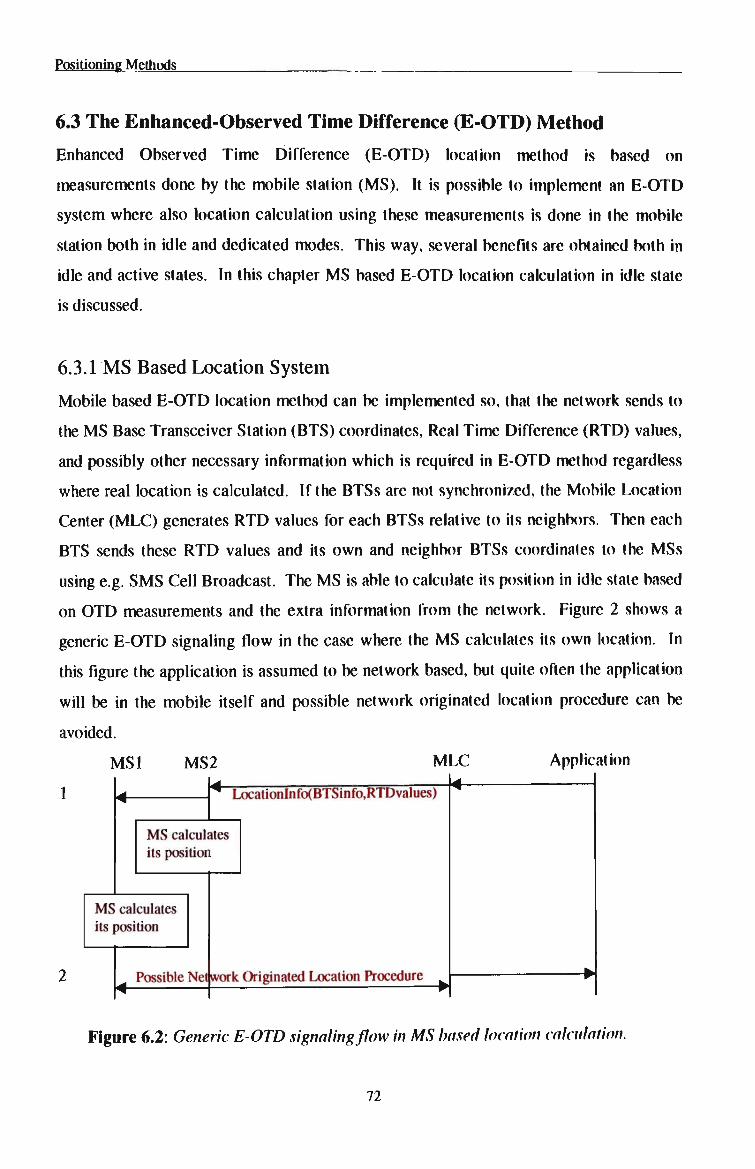
Positioning Methods
6.3 The Enhanced-Observed Time Difference (E-OTD) Method
Enhanced Observed Time Difference (E-OTD) location method is based on
measurements done by the mobile station (MS). It is possible to implement an E-OTD
system where also location calculation using these measurements is done in the mobile
station both in idle and dedicated modes. This way, several benefits are obtained both in
idle and active states. In this chapter M S based E-OTD location calculation in idle state
is discussed.
6.3.1 MS Based Location System
Mobile based E - O T D location method can be implemented so, that the network sends to
the M S Base Transceiver Station (BTS) coordinates, Real Time Difference (RTD) values,
and possibly other necessary information which is required in E-OTD method regardless
where real location is calculated. If the BTSs are not synchronized, the Mobile Location
Center (MLC) generates R T D values for each BTSs relative to its neighbors. Then each
BTS sends these R T D values and its own and neighbor BTSs coordinates to the MSs
using e.g. S M S Cell Broadcast. The M S is able to calculate its position in idle state based
on O T D measurements and the extra information from the network. Figure 2 shows a
generic E-OTD signaling flow in the case where the M S calculates its own location. In
this figure the application is assumed to be network based, but quite often the application
will be in the mobile itself and possible network originated location procedure can be
avoided.
M S I M S 2 M L C Application
_
^ ^ Lnr alues)
M S calculates
its position
M S calculates its position
_ Possible Net (̂
work Originated Location Procedure _
[M
_ w
Figure 6.2: Generic E-OTD signaling flow in MS based location calculation.
72

Positioning Methods
In figure 6.2 it has been assumed that:
1. The MLC calculates the RTD values for all BTSs and each BTS transmits these RTD
values and its neighbor's coordinates. If the BTSs are not synchronized, the R T D values
must be sent periodically to the M S . The R T D sending frequency depends on the quality
of the network synchronization (the updating frequency could be for example in the order
of 1-2 minutes). The extra information from the network can be encrypted so that only
those M S subscribers, that have subscribed for M S based E - O T D location calculation
service, can decode the information. This enables operators to charge for location
service.
2. Some network based application may request the location of the MS either directly or
through M L C .
6.3.2 Benefits and Applications
The above described system enables the M S to calculate continuously and real time its
own position using O T D measurements. There would be no need to have active two-way
communication with network at all, i.e., additional network signaling capacity would not
be needed, all required measurements and data could be obtained in idle mode. The
continuous O T D location calculation in M S makes possible to improve the location
accuracy, e.g. by having continuously running filtering. The M S can also obtain
information about its movements.
The location is therefore available for the MS at all times, continuously in idle mode and
when in call mode. Possible applications for this continuos location will be chart
applications, tariff applications (e.g. home zone) and location information could be also
one tool for Mobile Execution Environment (MexE).
Location calculation in MS offers several benefits for tariff applications:
• Tariff zones are easier to provision (e.g. subscribers home's coordinates can be used,
there is no need to do any activation measurements).
73

Positioning Methods
• Tariff zones are easier to maintain, there in no need to worry about new B T S coverage
areas, i.e. the zones can be separated from G S M network topology.
• Smaller and more reliable zones are possible.
• User indication is possible, i.e. he or she can be notified continuously, also in idle state,
whether he or she is inside special tariff zone.
The operator will benefit from the increased traffic generated by these new applications
which are using M S based location. Also the operator's tariff applications will work
better: e.g. in home zone service the cheap home zone tariff can be given to much smaller
area than using only CI, and simultaneously the reliability will be high and thus the end
users will be more satisfied to this service. Additionally, the operator controls the
coordinates of the base station and R T D values, so the use of M S based location
calculation service can be charged.
6.3.3 E-OTD Computations
When time of arrival measurements are made in an uplink or a downlink based method,
assuming some knowledge about the synchonisation state of the network, the differences
of time of arrival called also E - O T D are made. The aim of this section in the thesis is to
explain the E - O T D positioning method and to show that some cautions must be taken
while computing the E-OTD. The location procedure can be divided into 2 processes PI
andP2:
Pi P2 TOA_l,TOA_2,...,TOA_n — • E - O T D J , E-OTD_2 E-OTDJn-l) - > x,y)
PI: E-OTD computations from the TOA measurements in the mobile or the base
station. For n T O A measurements correspond («-1) E-OTD, n>2 in case of 2
dimensions.
P2: Estimation of the x and y coordinates by an algorithm of triangulation.
If some confidence values of the TOA parameters are computed, then for each E-OTD
the confidence value will be, for example, the sum of the 2 confidence values of the
74

Positioning Methods
corresponding T O A . If such confidence values are available and well-computed, the
precision of the final location can be enhanced.
6.3.3.1 CramCr-Rao bound
This bound shows the best performance that the estimator can reach. As 2 parameters
need to be estimated, x and y, the bound is given by a matrix with 2 dimensions. The
bound on each parameter to be estimated is given by the diagonal elements of this matrix.
W h e n performing a location trial with n base stations, this bound depends on the
coordinates, x and y, of the mobile :
r(J2x(x,y) a\x,y))
a(x,y) <r2y(x,y) CRBn(x,y) =
The resulting variance is simply the sum of the diagonal elements of this matrix. The
expectation of the precision over the whole network is chosen to be computed. The mean
value of the error over all the pixels in the network is computed assuming that the E - O T D
are all gaussian zero mean and decorrelated. Borders effect are not considered. It can be
shown that:
RMS. \]^l+a2ydxdy J^ _jjjTr[CRB„(x,y)frxdy J^
jjdxdy fjdxdy
The simplest way to compute the E - O T D is the following:
E-OTD_\ E-OTD _2
E-OTD _(«-!)
=
-1 1 0 0 0 -10 1 0 0
-10 0 0 1
TOA_\ TOA_2
TOA_n
The E-OTDs are computed according to the base station to which the mobile is
connected. The idea behind that is the fact that the link between this base station and the
mobile is the best one in term of signal strength.
75

Positioning Methods
Another scheme of computing the E-OTD is the following:
E-OTD_\ E-OTD _2
E-OTD _(n-l)
-1 1 0 0 0
0 - 1 1 0 0
0 0 0-11
TOA_
TOA_
TOA_
_f .2
,n
In this case each E-OTD depends on the last 2 T O A measurements. The consequence of
this definition is that the E-OTDs have better correlation properties.
76

Position Calculations and Statistical Evaluation
CHAPTER 7 POSITION CALCULATIONS AND STATISTICAL EVALUATION
7.1 Introduction
The position calculation function utilises the available measurements, e.g., T O A
measurements from three or more B S - M S links, to produce a position estimate. The
statistical evaluation is based on computing the difference between the estimated
position, given as:
A A
EstimatedPostion = (x,y)
and the true position of the mobile station, given as:
True position = (x,y).
Statistics on the circular error could be presented by plotting the cumulative distribution
function (CDF) of absolute location error. Another possibility is to compute the root
mean square error (rmse), which is given by the following equation:
I1 V rmse = J — >
(x.-x,.)2+(y,.-y,) 2^
)
Where N is the total number of positioned mobile stations. The rmse calculation is very
sensitive to occasional poor estimates (caused for example by poor measurements or lack
of measurements). A measure which is less sensitive to these rare so-called outliers is
obtained by omitting a fraction of MS's (e.g., 10%) which are the worst cases in the rmse
calculation.
Due to the modular structure of the simulator, it is possible to study the different aspects
of system simulation, link level simulation (e.g., T O A estimation) and position
calculation not only integrated but also separately. Analysis of the output of the radio
network simulator allows investigations of the expected Carrier / (Interference+Noise)
values at serving and neighboring BS's for different parameters, e.g., cell radius or
77
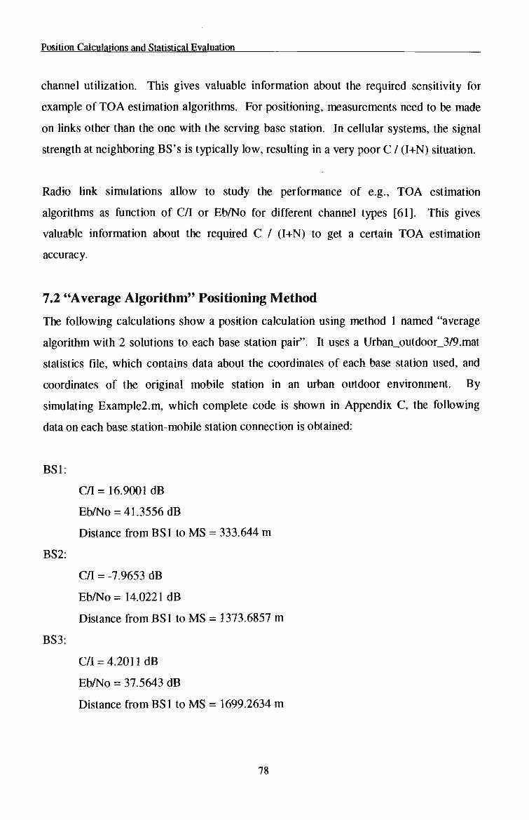
Position Calculations and Statistical Evaluation
channel utilization. This gives valuable information about the required sensitivity for
example of T O A estimation algorithms. For positioning, measurements need to be made
on links other than the one with the serving base station. In cellular systems, the signal
strength at neighboring BS's is typically low, resulting in a very poor C / (I+N) situation.
Radio link simulations allow to study the performance of e.g., TOA estimation
algorithms as function of C/I or Eb/No for different channel types [61]. This gives
valuable information about the required C / (I+N) to get a certain T O A estimation
accuracy.
7.2 "Average Algorithm" Positioning Method
The following calculations show a position calculation using method 1 named "average
algorithm with 2 solutions to each base station pair". It uses a Urban_outdoor_3/9.mat
statistics file, which contains data about the coordinates of each base station used, and
coordinates of the original mobile station in an urban outdoor environment. By
simulating Example2.m, which complete code is shown in Appendix C, the following
data on each base station-mobile station connection is obtained:
BS1:
C/I = 16.9001 dB
Eb/No = 41.3556 dB
Distance from B S 1 to M S = 333.644 m
BS2:
C/I = -7.9653 dB
Eb/No = 14.0221 dB
Distance from BS1 to M S = 1373.6857 m
BS3:
C/I = 4.201 ldB
Eb/No = 37.5643 dB
Distance fromBSl to M S = 1699.2634 m
78

Position Calculations and Statistical Evaluation
Using bsv(ms,bs), which is an output array from the System Simulator, the three base
station coordinates and the original mobile station coordinates could be obtained. In this
particular case they are as follows:
bsv(ms,l) = 19. This means first base station used in this calculation is equal to the 19th
base station out of the statistics file. The m s indicates mobile station, which is equal to 1
due to the fact that only one mobile station is to be positioned. Therefore x and y
coordinates of the 19th base station are obtained using the array xyb(ms, bs).
N o w , xyb(l,19) = xyb(ms, 1st base station) = (0,0).
In the same manner the other two base station coordinates are obtained, where:
xyb(ms, 56) = xyb(ms, 2nd base station) = (1500, -2.27* 10"13) and
xyb(ms, 3rd base station) = (750, -1299).
The mobile station coordinates are obtained using the array xym. The are 750 mobile
positions to choose from, indicating a moving mobile. The first mobile position is used
in this particular calculation, which is x y m = (158.1, 293.81). All position measurements
above are given in metres.
BSs & Original MS 400
200
-200 Dis tan ce -400 (m)
-600
-800
-1000
-1200
-1400 500 1000
Distance (m) 1500
Figure 7.1: Three Base Stations & Original Mobile Station.
79

Position Calculations and Statistical Evaluation
Figure 7.1 shows all base stations and the original mobile station according to their x and
y coordinates. The blue circles indicate the 3 base stations and the green circle is the
mobile station.
This method for position estimation uses only two base station at one given instant to find
a mobile position. In fact two solutions are obtained from a pair of two base stations.
For example, out of the 3 base station shown in figure 1, BS1 and B S 2 will be involved in
the calculation to obtain two solutions. Once the two solutions have been obtained, B S 1
and BS3 are used, for 2 more solutions, and finally BS2 and BS3 for another 2 solutions.
When all base station have been involved, a total of six solutions are obtained, providing
there is a 3 base station system in the calculation.
Shown below is the calculation method for BS1 and BS3.
This original mobile station sends uplink signals to the operating base stations. For each
sent signal, the estimated time of arrival (TOA) is calculated according to formulas given
in chapter 6. For the signal to reach BS1 from the M S it takes approximately 1.0 psec
and 4.2 usee from B S 2 to M S . Therefore from this, the distance for each connection
could be calculated using the relationship:
d = c * t (7.1)
where c is the speed of light equal to 3* 108 and t is the T O A estimate.
So, M S to B S 1 = 1.0 usee.
Therefore d = c * t
d. = (3*108)*(1.0psec)
di = 300 metres
For MS to BS2 = 4.2 psec.
Therefore d = c * t
d2 = (3*108)*( 4.2 psec)
d 2 = 1260 metres
By substituting the above distances in the following two equations, 2 mobile estimated
positions could be obtained.
80

Position Calculations and Statistical Evaluation
Equation 1:
(Xm-XBSl) + (Yra-YBSl) = di (7.2)
Equation 2:
(Xm-XBS2) + (Y„,-YBS2) = d2 (7.3)
By simultaneously solving the above two equations, two solutions are obtained. With
BS1 and B S 2 operating the two solutions are as follow:
Estimated mobile position 1:
Xmi = 250.8
Ymi = 164.6188
Estimated mobile position 2:
Xm2 = 250.8
Ym2=-164.6188
Refer to Appendix D, location.m file for complete solution to the 2 equations.
These positions are shown in figure 7.2 below, indicated by the red circles.
400
200
0(
Dis -200
tan ce -400 (m)
-600
-800
-1000
-1200
-1400
Base Station 1 & Base Station 2 operating
•
•
t
m
•
1
500 1000 Distance (m)
1500
Figure 7.2: Position estimates with BS1 & BS2 operating.
Similarly, two other positions could be obtained when BS1 and BS3 are operating. For
BS3, it takes approximately 5.2 psec for the signal generated by the M S to reach BS3.
Therefore using equation 7.1, distance from BS3 to M S is equal to 1560 meters. Other
81

Position Calculations and Statistical Evaluation
data required to obtain the two estimated positions is BS3 x and y coordinates. As
mentioned earlier, they are:
X Y B S 3 = (750, -1299)
With this data, the two estimated mobile positions, with BS1 and BS3 operating could be
obtained using equations 7.2 and 7.3. The two solutions are listed below.
Estimated mobile position 1:
X mi = 242.7766
Y m l = 176.2371
Estimated mobile position 2:
X m 2 =-274.0110
Ym2=-122.1391
Figure 7.3 below shows these estimated mobile positions, together with the original
mobile position and the three base stations.
Base Station 1 & Base Station 3 operating 400
200
-200| Dist anc -40 r; e (m) -600
-800
-1000
-120C
-140* 400 -200 0 200 400 600 800 1000 1200 1400 1600
Distance (m)
Figure 7.3: Position estimates with BS1 & BS3 operating.
Again the blue circles indicate the three base station, the green circle is the original
mobile station and the two red circles indicate the estimated mobile positions. In the
82

Position Calculations and Statistical Evaluation
same manner as above two estimated mobile positions are obtained for BS2 and BS3
operating.
The time of arrival from M S to BS1 is already known to be 1.0 usee, giving a distance of
300 metres, and a time of 5.2 usee from M S to BS3, giving a distance of 1560 meters.
Therefore once again by simultaneously solving equations 7.2 and 7.3, the following
estimated positions are obtained.
Estimated mobile position 1:
Xmi = 252.8760
Y m l = 179.6709
Estimated mobile position 2:
X m 2 = 2279.1
Ym2=-990.2254
Figure 7.4 shows the graphical representation of the above positions.
Base Station 2 & Base Station 3 operating
DIs tan ce (m)
400
200
Oi
-200
-400
-600
-800
-1OO0
-1200
-1400
___
, f,
•
500 1000 1500 Distance (m)
2000 2500
Figure 7.4: Position estimates with BS2 and BS3 operating.
From the six estimated mobile positions, the average is taken and is considered to be the
final estimated mobile position.
83

Position Calculations and Statistical Evaluation
Average position = (sum of all positions) / the number of positions.
For the above case average position is equal to the following:
Average mobile position: XYMs = (500.3906, -126.1876).
This is shown in figure 7.5 below.
400
200
0*
-200
400
-600
-800
-1000
-1200
-1400 0 500 1000
Distance (m)
DIs tan ce (m)
(
1500
Figure 7.5: Average estimated mobile position for a 3 BS system.
The circular error for the above case could be obtained using the below formula:
rmse •M (*,.-*,.)2+(y,.-y(.)
2
where N = number of mobile stations to be positioned, N = 1.
Oft y,) = (158.1, 293.81), A A
(*,»y() = (500.3906,-126.1876).
By substituting the above values in the equation a rms. error of 696.99 meters is obtained.
An average mobile location error could not be accurately obtained by one set of
simulation. Due to this fact a set of 30 different mobile locations has been simulated
giving an average rms. error of 645 metres, for the three base station system.
84

Position Calculations and Statistical Evaluation
In exactly the same fashion as for a three base station system, a five base station system
was simulated, giving a more accurate mobile position. The root mean square error was
obtained to be 281.8 metres. The graphical representation for a five base station system
is shown in figure 7.6 below.
Average Position Estimate, 5 BS System
1500
1000
500 Dis tan ce (m) 0
-500
-1000
-1500 -1000 -500 0 500
Distance (m) 1000 1500
Figure 7.6: Average estimated mobile position, for a 5 BS system.
As it can be noticed, with an increase of base stations numbers, a more accurate
estimation could be achieved.
With a 7 base station system the circular error was obtained, after 30 sets of simulations,
at different mobile locations. The average estimated mobile position was worked out to
be as shown below:
Average estimate: XYMs = (81.3563,46.4616).
Using this estimate, the root mean square error obtained was:
rmse = 258.98 metres.
Figure 7.7 shows this graphically.
85

Position Calculations and Statistical Evaluation
Di sta nc e (m
1000
500
-500
-1000
.icnn
1
Average Position Estimate, 7 BS System
•
•
•
(F
•
•
it
-1500 -1000 -500 0 500 Distance (m)
1000 1500
Figure 7.7: Average estimated mobile position, for a 7 BS system.
7.3 "More Preferable Solution" Positioning Method
I would now like to propose another method named "more preferable solution". The way
the method operates is that, out of the two solution obtained as described in this chapter
above using method 1, only one "more preferable" solution is taken, and the average is
calculated as shown below:
* 1 n
* = -_£*; K ] n
y=-"Ly< nti
where n is the number of pairs considered.
The question may arise of how to choose a "more preferable" solution, out of the two
possible solutions obtained by using method 1. The more preferable solution is chosen
according to a distance from a third base station, which needs to be included in the
calculation.
Consider Figure 7.8. Here, a three base station system is considered. W h e n BS1 and
BS2 are operating, BS3 is used to help decide which estimated position is closer to the
86

Position Calculations and Statistical Evaluation
mobile station. W h e n BS2 and BS3 are operating, which means that they are used to get
two estimated positions, like in method 1, then BS1 is used for making a decision.
Estimated position 1
BS2
LBS2
mated position 2
BS3
Figure 7.8: Three base station system, Method 2, with BS3 deciding.
The more preferable solution is chosen according to the following 2 rules:
if I mi-LBs3 I < I m2-LBs3 I then choose Estimated position 1.
if I mi-LBs31 > I m2-LBs3 I then choose Estimated position 2.
In this method n = N/2, where N is a number of points in method 1. It should be noted
that, if the number of base station is greater than 3, any one (only one) base station could
be chosen for making the decision, while the two base stations are operating.
The MATLAB file that selects which is a more preferable pair is described below.
% Method 2 MATLAB file % The file currently uses BS1 & BS2 as the two operating BS's, and BS3 % is used to make the decision.
Xel =250.8; % x coordinate of Estimated position 1, Yel = 164.6188; % y coordinate of Estimated position 1.
Xe2 = 250.8; % x coordinate of Estimated position 2 Ye2 = -164.6188; % y coordinate of Estimated position 2
Xbs3 = 750; Ybs3 = -1299;
% x & y coordinates of base station used for making % the decision.
87
Position Calculations and Statistical Evaluation
L_bs3 = 1560; % Distance of the decision making BS to MS. % obtained by using the TOA method.
ml = sqrt( ((Xel-Xbs)*(Xel-Xbs)) + ((Yel-Ybs)*(Yel-Ybs)) ); m2 = sqrt( ((Xe2-Xbs)*(Xe2-Xbs)) + ((Ye2-Ybs)*(Ye2-Ybs)) );
if (abs(ml-L_bs) < abs(m2-L_bs)) sprintf('The position is Xel=%d,Yel=%d\n',Xel,Yel)
else sprintf('The position is Xe2=%d,Ye2=%d\n',Xe2,Ye2)
end
As it can be seen in the file itself, the input values currently in it are: BS1 & B S 2
operating, and B S 3 is used for decision making. With a slight change to the input values,
any pair could be input, to obtained a wanted solution.
After executing the above file, the estimated position selected is: Estimated position 1,
which very clearly can be seen that this position is closer to the original MS than the
estimated position 2. Figure 7.9 shows the graphical representation on this position.
Base Station 1 & Base Station 2 operating, BS3 used as a decision making BS.
400
200
0i
Dis tan ce (m)
-200
400
-600
-800
-1000
-1200
-1400 500 1000
Distance (m)
1500
Figure 7.9: BS1 & BS2 operating, while BS3 makes the decision, 3 BS system.
If Figure 7.9 is compared with Figure 7.2, it can clearly be seen that the Estimated
position 2, which is shown in Figure 7.2, is ignored in Figure 7.9 with the help of the
88

Position Calculations and Statistical Evaluation
above M A T L A B file. Once again in Figure 7.9, the blue circles are the three base
stations, the green is the original M S and the red is the estimated M S .
For this particular case, when BS1 and B S 2 are operating, and BS3 is used for decision
making, the estimated position is: (250.8,164.6188), as shown in Figure 7.9.
When BS1 and BS3 are operating, and B S 2 is used for decision making, the estimated
position is: (242.7766,176.2371), as shown in Figure 7.10 below.
Base Station 1 & Base Station 3 operating, BS2 used as a decision making BS. 400
200
Dis tan ce (m)
-200
-400
-600
-800
-1000
-1200
-1400 500 1000 1500
Distance (m)
Figure 7.10: BS1 & BS3 operating, while BS2 makes the decision, 3 BS system.
When BS2 and BS3 are operating, the decision making base station is BS1. In this case
the estimated mobile position is: (252.8760, 179.8709), as shown in Figure 7.11. Base Station 2 & Base Station 3 operating, BS1 used as a decision making BS.
400
200
Oi
-200 Dis tan ce -400 (m)
-600
-800
-1000
-1200
-1400
•
_. -
»
3 5<
•
)0 Distance (m)
10
1 j
00 151
Figure 7.11. BS2 & BS3 operating, while BS1 makes the decision, 3 BS system.
89
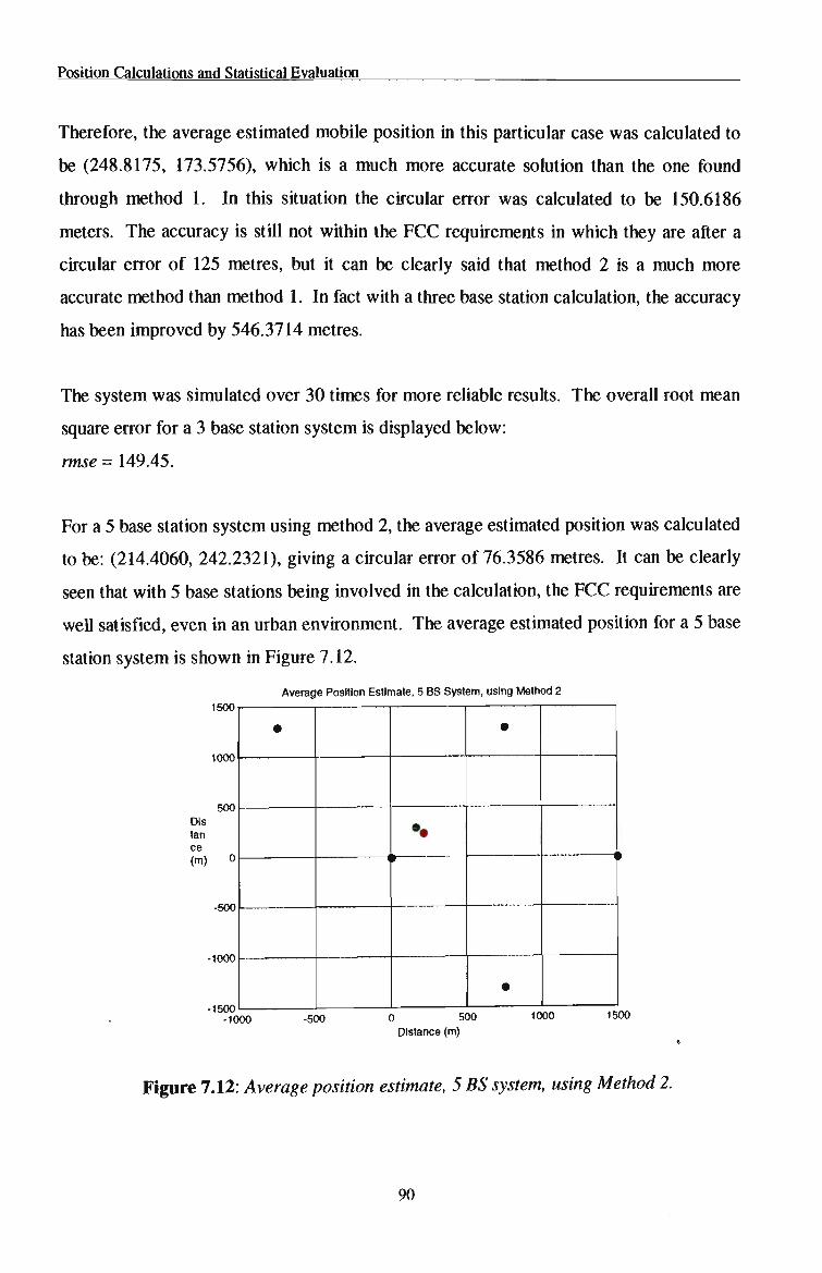
Position Calculations and Statistical Evaluation
Therefore, the average estimated mobile position in this particular case was calculated to
be (248.8175, 173.5756), which is a much more accurate solution than the one found
through method 1. In this situation the circular error was calculated to be 150.6186
meters. The accuracy is still not within the F C C requirements in which they are after a
circular error of 125 metres, but it can be clearly said that method 2 is a much more
accurate method than method 1. In fact with a three base station calculation, the accuracy
has been improved by 546.3714 metres.
The system was simulated over 30 times for more reliable results. The overall root mean
square error for a 3 base station system is displayed below:
rmse = 149.45.
For a 5 base station system using method 2, the average estimated position was calculated
to be: (214.4060, 242.2321), giving a circular error of 76.3586 metres. It can be clearly
seen that with 5 base stations being involved in the calculation, the F C C requirements are
well satisfied, even in an urban environment. The average estimated position for a 5 base
station system is shown in Figure 7.12.
Average Position Estimate, 5 BS System, using Method 2
1500
1OO0
500 Dis tan ce (m)
-500
-1000
-1500
, , ,,
-1000 -500 0 500 Distance (m)
1000 1500
Figure 7.12: Average position estimate, 5 BS system, using Method 2.
90

Position Calculations and Statistical Evaluation
For a 7 base station system, the average estimated mobile position using method 2 was
calculated to be (187.046, 247.851), giving a circular error of only 54.31 metres. This
results suggests that the FCC requirement of a circular error of 125 meters is well beaten.
The average estimated position, using method 2 is displayed in Figure 7.13.
Average Position Estimate, 7 BS System, using Method 2 1500
1000
500 Di sta nc e (m
0*
-500
-1000
-15001
-1500 -1000 -500 0 500 Distance (m)
1000 1500
Figure 7.13: Average position estimate, 7 BS system, using Method 2.
As this chapter has shown, an increase in base station numbers gives a more accurate
mobile position. But to satisfy the FCC requirements obviously a more accurate method
needs to be defined, like method 2. Method 2 has satisfied the FCC requirements very
well, giving a final circular error of only 54.31 meters, with a 7 base station calculation.
Chapter 8 introduces another method, method 3, named "Enhanced Fuzzy Method",
which tries to improve the position accuracy to a greater degree.
91

Fuzzy Logic Positioning
CHAPTER 8 FUZZY LOGIC POSITIONING
8.1 Introduction to Fuzzy Logic
Fuzzy set theory, introduced by Zadeh [62] in 1965, has been shown to be an effective
way to deal with qualitatively oriented terms and concepts. Fuzzy logic provides a
simple way to draw definite conclusions from vague, imprecise information. In an
intuitive sense, it resembles assertion concerning a mobile unit traveling on a local
residential road:
" The speed of this mobile unit is high."
If the speed is 100 km/h, this statement is completely true. However, if 100 km/h is high,
how about 99, 98, ... 90, ... 80, ... 70? At what degree does the statement suddenly
become false? Since the speed can be changed gradually during a trip, it is hard to find a
fixed value such that larger than that fixed value is "high" and less than that value is "not
high". To resolve this fuzziness, a grade or a membership degree could be assigned to a
certain speed. B y correlating various speeds to grades, w e turn the preceding statement
into a fuzzy membership function. Therefore, it has often been said that fuzzy logic is a
mathematical formalism intended to handle these kind of imprecise statements. It is
different from traditional mathematical formalisms because fuzzy logic allows the user to
model the vagueness in their mental decision-making process. Consequently, fuzzy logic
is intuitive and easier to work with than traditional logic for many applications.
Traditional logic would have a difficult time processing for the given statement. In the
design of fuzzy inference system, there are three basic concepts: membership functions,
fuzzy logic operations, fuzzy rules.
For membership functions, it can be denoted that the grade of a speed in high by
assigning it a numerical "truth value". Truth-values may range anywhere between 0 and
1, and are typically considered to have meaning as suggested in Table 8.1, although it
may not always have meaning. In this manner various grades could arbitrarily be
assigned to "high" as a function of the speed, as shown in Table 8.2.
92

Fuzzy Logic Positioning
The membership functions given in the tables are illustrated in Figure 8.1. The curve in
the Figure 8.1 illustrated how the membership function of a fuzzy concept is dependent
on a measured value, for example, speed. W h e n the relevant declarative assertions are
combined into a single chart, more complicated curves are obtained. These curves are
called fuzzy sets. The fuzzy concept "high" is called a label. For a speed such as 70
km/h, 0.7 is its grade in high. In other words, if the speed of this mobile is 70 km/h, the
truth-value of the assertion "The speed of this mobile is high" is 0.7.
Truth Value
0.0
0.2
0.4
0.6
0.8
1.0
Meaning
Completely false
Mostly false
Somewhat false
Somewhat true
Mostly true
Completely true
Table 8.1: Linguistic meanings of fuzzy logic values.
Speed (km/h)
0
10
20
30
40
50
60
70
80
90
100
Grade in high
0.0
0.1
0.2
0.3
0.4
0.5
0.6
0.7
0.8
0.9
1.0
Table 8.2: Membership function
93

Fuzzy Logic Positioning
Grade
1 1 1 r~ ~ Speed
20 40 60 80 100
Figure 8.1: Membership function chart.
For fuzzy logic operations, consider the spoken language. In additional to the simple
assertion statement presented earlier, logic operations are often used in spoken language
to combine simple assertions into complex ones. Examples of such operators are " A N D "
and "OR". Assertions using these operators are called compound assertions. Similar
operators could be used in fuzzy logic to help evaluate the truth-values of these
assertions. These operations are called fuzzy logic operations. For example, another
simple assertions could be defined:
" The distance to the next maneuver is short."
A compound assertion can now be created:
" The speed of this mobile is high A N D the distance to the next maneuver is
short."
Once a truth-value is assigned to each simple assertion, fuzzy logic operations can
precisely evaluate the truth-values of compound assertions. Even though the compound
assertion is vague, the evaluation results are crisp value. In other words, nothing is fuzzy
in the actual fuzzy inference process.
As examples, how to evaluate truth values for statements containing the two simple
operators, A N D or O R could be examined. Mathematical functions are used by fuzzy
logic to evaluate two arbitrary statements A and B. These statements can be either simple
94

Fuzzy Logic Positioning
or compound. The mathematical functions are listed in the right-hand column of Table
8.3. Each of them is associated with its corresponding operator in the left-hand column.
Compound operator on
Statements A and B
AANDB
A ORB
Mathematical functions to
evaluate truth
minimum (min)
maximum (max)
Table 8.3: Fuzzy logic operations.
From the definitions given in Table 8.3, the truth-value of any statement could easily be
evaluated. If the truth value of A is 0.1 and the truth value of B is 0.8, the following
could be obtained:
Assertion 1: A AND B = min(0.1, 0.8) = 0.1
Assertion 2: A OR B = max(0.1, 0.8) = 0.8
The crisp truth-value of assertion 1 is 0.1, whereas assertion 2 has a value of 0.8. It could
be now known that a traditional logic such as Boolean logic is a special case of fuzzy
logic. If there is any doubt about this statement, refer to Table 8.4, which lists various
evaluation results for two compound assertions.
Logic Operator
A
0
0
1
1
0
0.5
0.8
1
B
0
1
0
1
0.6
0.5
0.6
0.6
Fuzzy Logic
AANDB
0
0
0
1
0
0.5
0.6
0.6
A ORB
0
1
1
1
0.6
0.5
0.8
1
Boolean Logic
AANDB
0
0
0
1
7
7
7
?
A ORB
0
1
1
1
7
?
?
7
Table 8.4: Comparison of Boolean Logic and Fuzzy Logic Operations.
95
Fuzzy Logic Positioning
Both results obtained by applying fuzzy logic operators and Boolean logic operators are
derived. It should be noted that both fuzzy logic and Boolean logic produce the same
results when truth-values of the simple assertions are limited to 1 and 0. However, for
values other than 1 or 0, fuzzy logic produces meaningful results while Boolean logic has
no such operations defined.
For fuzzy rules, the following example could be considered. Suppose that the task is to
determine when to announce a maneuvering instruction to a travelling mobile user during
route guidance. One of the rules could be:
IF the speed of the travelling mobile is high AND the distance to the next
maneuver is short
T H E N announce the next maneuver instruction.
In other words, a rule has the following format:
IF <condition> T H E N <consequence>.
The condition part of a rule could be either a simple or compound statement and the
consequence part is typically a simple statement. The input to a fuzzy-logic-based
system is very similar to human language. The more complex a system is, the more rules
it will generally have. Given the input grades in the condition part, each rule is evaluated
to obtain an output grade in the consequence part.
The final result of this inference process depends on the combinational effect of many
fuzzy rules in the process. Due to the fact that a single number is desired at the output, a
defuzzifying operation is required. In other words, a defuzzification operator is used to
compute one final crisp output value, which is to make a decision for the system to
follow. The final step could be viewed as interpreting the evaluated grades as a measure
of confidence in the corresponding conclusion. The most popular method used for this
operation is to compute the centroid (weighted average) of the output from the fuzzy
rules. B y considering the grades as weights attached to the assertions, the final decision z
is obtained by determining the weighted average of the support values associated with
each output label.
96

Fuzzy Logic Positioning
The final decision z is defined by the following formula:
Z = ^-___-
where JC is the position of the fuzzy output from the evaluation, y is the value (weight) of
the corresponding fuzzy output, and n is the number of fuzzy outputs. In general, the
outputs of fuzzy rule evaluation results are discrete values. For convenience, a curve is
used in Figure 8.2 to explain the basic concept.
Y
One Fuzzy Output Value
Figure 8.2: Example of a fuzzy output curve.
8.2 Enhanced Fuzzy Positioning Method
As method 2 in chapter 7 proved the F C C requirements of a circular error of 125 metres
has well beaten. This section uses the fuzzy background, described in section 8.1 to
produce a more accurate method 3, named "Enhanced Fuzzy Method". The method uses
the above formulas, which has been derived according to the formula above, defined by
z.
The method computes the weighted average of the output, where the output is the bit
energy to noise power spectral density ratio, Eb/N0, as described in chapter 4. The
method uses similar assertions as described in section 8.1. Let's have a look at the
following 3 base station system The same values have been used in the calculations of
method 1 and method 2, described in chapter 7. Consider the below figure, Figure 8.3.
97

Fuzzy Logic Positioning
BS/
BST
• B S C
Figure 8.3: Base station-Mobile station connections.
Assertion 1 would be a solution of BSA and BSB operating. Assertion 2 is a solution of
B S A and BSc operating, and assertion 3 is a solution of B S B and BSc operating. Consider
the following assumptions:
T A = bit energy / noise power spectral density ratio from B S A
r B = bit energy / noise power spectral density ratio from B S B
T c = bit energy / noise power spectral density ratio from BSc
Now using the above assumptions and the fuzzy theory described in section 8.2, the
weights for the three B S - M S connections could be worked out.
ri = max(rA,rB)
r2=max(rA,rc)
r3=max(rB, rc)
From these values, the weighted values for each connection is worked out according to
the following formula:
' 50
Because W4 is a belief degree to a certain solution, it is chosen to be displayed in a range
between 0 and 1. (0 < W , < 1). The highest bit energy to noise power spectral density
ratio possible is 50 dB, therefore Tj is divided by 50 to get a belief degree between 0 and
1.
98
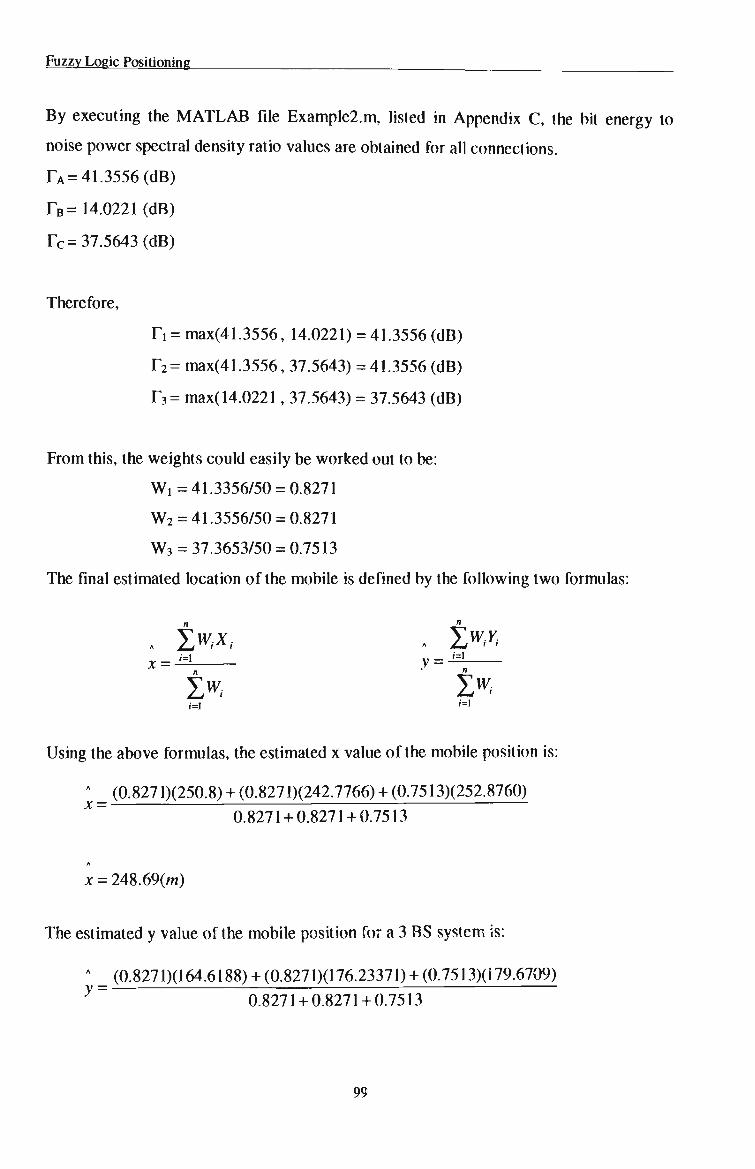
Fuzzy Logic Positioning
By executing the M A T L A B file Example2.m, listed in Appendix C, the bit energy to
noise power spectral density ratio values are obtained for all connections.
T A = 41.3556 (dB)
T B = 14.0221 (dB)
T c = 37.5643 (dB)
Therefore,
H = max(41.3556, 14.0221) = 41.3556 (dB)
T 2= max(41.3556, 37.5643) = 41.3556 (dB)
T3= max(14.0221, 37.5643) = 37.5643 (dB)
From this, the weights could easily be worked out to be:
W . = 41.3356/50 = 0.8271
W 2 = 41.3556/50 = 0.8271
W 3 = 37.3653/50 = 0.7513
The final estimated location of the mobile is defined by the following two formulas:
. ±wtxt „ ±W,Y, x=±* y=___
Using the above formulas, the estimated x value of the mobile position is:
A _ (0.8271)(250.8)+ (0.8271)(242.7766)+ (0.7513)(252.8760)
0.8271 + 0.8271 + 0.7513
A
x = 248.69(m)
The estimated y value of the mobile position for a 3 BS system is:
A _ (0.8271)(164.6188) + (0.8271)(176.23371) + (0.7513)(179.6709) y~ 0.8271 + 0.8271 + 0.7513
99

Fuzzy Logic Positioning
y = 173.3150(m)
Therefore, for a three base station system, the average estimated mobile position using
the enhanced fuzzy method is (248.6900, 173.3150). The position is shown in Figure 8.4
below.
400
200
0.
Dis "20° tan ce -400 (m)
-600
-800
-1000
-1200
-1400
Average Position Estimate, 3 BS System, using Fuzzy Method
500 1000 Distance (m)
1500
Figure 8.4: Average position estimate, 3 BS system, using fuzzy method.
The circular error for a 3 base station system is as follows:
rmse = V(158.1 - 248.69)2 + (293.81 -173.31)2
rmse = 150.75 (m)
where Original M S position, labeled green = (158.1, 293.81).
The system was simulated over 30 times for a more reliable result. The overall circular
error of the enhanced fuzzy method for a 3 B S system was obtained to be 148.76 metres.
In the same manner, a 5 base station system was simulated according to a weighted
average of the bit energy / noise power spectral density ratio. The final estimated average
100

Fuzzy Logic Positioning
position was worked out to be at x = 211.9476, and y = 237.57. This point is shown in
Figure 8.5.
Average Position Estimate, 5 BS System, using Fuzzy Method 1500
1000
500 Dis tan ce (m) 0
-500
-1000
-1500
%
-1000 -500 0 500 Distance (m)
1000 1500
Figure 8.5: Average position estimate, 5 BS system, using fuzzy method.
The circular error of this system was calculated to be 78.0025 metres.
Once again, for a more accurate and average error the system was simulated
approximately 30 times. The circular error of the overall system was calculated to be
75.9546 metres.
With 7 base stations involved in the calculation, the average estimated mobile position
was calculated to be located at x = 186.340 and y = 249.851, giving an overall circular
error of 52.25 metres, as shown below.
rmse =v<*<- * ) 2 + (y,-y) 2
rmse = Vd58.l-187.046)2 +(293081 - 249.851)'
101

Fuzzy Logic Positioning
rmse = 52.25 metres.
After simulating the system over 30 times, a final estimated average position was
obtained to be located at (185.45, 250.91). This point is shown in Figure 8.6. The
circular error was obtained to be 50.8760 metres.
Average Position Estimate, 7 BS System, using Fuzzy Method
uf
K)
\
m
m
%
•
•
-1500 -1000 -500 0 500 1000 1500 Distance (m)
Figure 8.6: Average position estimate, 7 BS system, using fuzzy method.
As it has been seen in chapter 7 and in chapter 8 of this thesis, the Federal
Communication Commission requirement of 125 metres circular error has been satisfied.
In fact, out of the three introduced methods in this thesis, the "Enhanced Fuzzy Method"
has provided the best possible results, in terms of mobile positioning. Conclusions and
results of all three methods are summarised in chapter 9.
102

Comparisons and Conclusions
CHAPTER 9 COMPARISONS A N D CONCLUSIONS
9.1 Introduction
As mentioned earlier in the thesis, the model is capable of extracting information on few
environments. The environments are as follow:
• Urban environment
• Suburban environment
• Rural environment
• Bad Urban environment
• Hilly environment
As this is the most difficult and interesting case requiring a lot of research, the
calculations in this thesis have concentrated only on Urban environment, which means
that signals have traveled through densely populated areas, which includes multi-story
buildings, offices and city centres. All methods have been simulated using the Urban
environment, leaving the other environments for future work in this area.
9.2 Technique and Results Comparison
The results of all three methods have been summarised below.
Method 1
This method is the original method that has been used by Ericsson to locate a mobile
station. It combines only two base stations at one time, and out of each pair there are two
solutions. Finally the average is taken out of all positions and one final mobile location is
obtained.
Number of
BS's
3
5
7
Circular error
(m)
>500
281.80
258.98
Difference in meters from
FCC's 125 (m) radius
+ >500
+ 156.80
+ 133.98
Perc. at 125m
[%]
24
37
48
Table 9.1: Result summary for method 1.
103

Comparisons and Conclusions
Method 2
This method for positioning chooses a more preferable solution out of the two solutions
obtained from each pair in method 1. The more preferable solution is chosen according
to a third base station, which helps chose the preferable solution. The results are
summarised in Table 9.2 below.
Number of
BS's
3
5
7
Circular error
(m)
149.45
76.35
54.31
Difference in meters from
FCC's 125 (m) radius
+ 24.45
- 48.65
- 70.69
Perc. at 125m
72
95
95
Table 9.2: Result summary for method 2.
Method 3
This method computes the weighted average of the output, where the output is the signal
to noise ratio, Eb/Nc, as described in chapter 4. The method uses assertions, which chose
the higher signal to noise ratio for a certain BS-MS connection, and assign a weight to it.
The weight is calculated according to the degree of greatness of the signal to noise ratio.
The higher the signal to noise ratio, the higher the weight on that particular connection.
The weight is in the range of 0 and 1. Results on this method are displayed below in
Table 9.3.
Number of
BS's
3
5
7
Circular error
(m)
148.76
75.95
52.25
Difference in meters from
FCC's 125 (m) radius
+ 23.76
- 49.05
- 72.75
Perc. at 125m
[%]
73
97
97
Table 9.3: Result summary for method 3.
104

Comparisons and Conclusions
9.3 Conclusions
Most terrestrial-radio-based systems generally have a minimum error of at least 150
metres. The worst systems may have errors of up to 2,000 metres. As mentioned earlier,
the performance of these systems often deteriorates when approaching urban canyon
areas. The methods introduced in this thesis have shown that even in an urban
environment, the results that have been achieved well satisfy the F C C requirement of a
circular error of 125 metres. One particular technology, which has been used in method
3, enhanced fuzzy logic, has proven to be a successful method in reducing the positioning
error. The difference in improvement is not great, in comparison with method 2, but
nevertheless improvement has been noticed using fuzzy logic.
Fuzzy Logic Control (FLC) algorithms contribute a powerful tool for handling mobile
communications problems. FLCs have provided noticeable performance improvements
in terms of reducing the number of handovers, over the conventional handover and
positioning techniques and they have demonstrated superb robustness under changing
conditions. However, maturely to the novelty of this research area, the theory of F L C
design is not yet well established in mobile communications. Researches around the
world are trying to find answers to the following questions:
1. How to determine the optimal range for the FLC variables?
2. O n which basis should the membership functions be determined in order to
get the best possible mobile location?
9.4 Future Work
Most studies of hybrid methods are needed to further improve mobile positioning. For
instance, one method to reduce the positioning error would be to implement filtering
techniques in the mobile device, which uses the relationship between carrier Doppler
phases measurements and range estimates changes. Interested readers can find
information on various other radio location technologies and systems in [631 and [64].
105

Comparisons and Conclusions
Many of these technologies have very promising potential for use in mobile location
applications.
Another method to reduce the circular error in positioning of a mobile unit base the
weighted average on the signal strength between the mobile that needs to be positioned
and operating base stations. Once the weights have been correctly split up, the use of
fuzzy logic could chose, which base station, has a higher signal strength, and decide to
use that base station.
Another method to reduce positioning error would be to use both, the signal to noise ratio
and the signal strength of a signal. In this case the weighted average could be chosen
using both of these measurements. Take the following as a guide.
Wi = WSi*Wri
Wi= Weighted average of a signal or total belief degree
WSi = Belief degree based on signal strength
W n = Belief degree based on signal to noise ratio.
The belief degree could possible be chosen in the following fashion:
Wi = m i n ( W S i , W n ) .
106
REFERENCES
[1] M.D. Yacob, "Foundations of Mobile Radio Engineering", Boca Raton, FL: CRC
Press, 1993.
[2] Federal Communications Commission, "Reports and Order and Further Notice of
Proposed Rulemaking, C C Docket No.94.102, Revision of the Commission's Rules
to Ensure Compatibility with Enhanced Emergency Calling Systems", Released July
26, 1996.
[3] J. Cisneros, D. Delly and L.A. Greenbaum, "An Urban Positioning Approach
Applying Differential Methods to commercial F M Radio Emissions for Ground
Mobile Use", Proceedings of ION 50th Annual Meeting, pp. 83-94, June 1994.
[4] D.C. Kelley, D.T. Rackley and V.P. Berglund, "Navigation and Positioning Systems
and Methods Using Uncoordinated Beacon Signals", United States Patent,
No.5173710, Dec. 1992.
[5] O. Grimland and B. Gudmundson, "Handover Strategies in Microcellular Systems",
in IEEE Vehicular Technology Conference, pp.505-510,1991.
[6] A. Murase, I.C. Symington and E. Green, "Handover Criterion for Macro Cellular
Systems", in IEEE Vehicular Technology Conference, pp.524-530,1991.
[7] R. Vijayan and J.M. Holtzman, "A Method for Analyzing Handover Algorithms", in
IEEE Trans, on Vehicular Technology, pp.251-356, Aug. 1993.
[8] W.R.Mende, "Evaluation of a Proposed Handover Algorithm for the GSM Cellular
Systems", 40th IEEE Trans, on Vehicular Technology, pp.264-269, 1990.
107

[9] S.T.S. Chia, R.J. Warburton, "Handover Criteria for City Micro Cellular Radio
System", 40th IEEE Trans, on Vehicular Technology, pp.276-281, 1990.
[10] S.T.S. Chia, "Handover Initiation and Control for Highway Microcells", Fourth
Nordic Seminar Mobile Radio Communications", D M R I V , June 1990.
[11] G. Falciasecca, M. Frullone, G. Riva, A.M Serra, "Comparison of Different
Handover Strategies for High Capacity Cellular Mobile Radio Systems", 39th IEEE
Trans, on Vehicular Conference, pp. 122-127,1989.
[12] B. Gudmundson and O. Grimlund, "Handover in Microcellular Based Personal
Telephony Systems", In S. Nanda and D.J Goodman, eds., Third Generation
Wireless Information Networks, pp. 187-203, Kluwer Boston, 1992.
[13] O.E. Kelly and V.V. Veeravalli, "A Locally Optimal Handover Algorithm", in 6th
IEEE International Symposium on Personal, Indoor and Mobile Radio
Communications (PIMRC95), pp.809-813, Toronto, Sep. 1995.
[14] M. Gudmundson, "Analysis of Handover Algorithms", IEEE 41st Trans. Vehicular
Conference, pp. 537-542, 1991.
[15] M.D. Austin and G.L. Stuber, "Direction Based Handover Algorithm for Urban
Macrocells", in IEEE Vehicular Technology Conference, pp. 101-105, Atlanta 1994.
[16] E. Hepsaydir and W. Yates, "Performance Analysis of Mobile Positioning Using
Existing C D M A Network", in IEEE Vehicular Technology Conference, pp. 190-192,
1994.
[17] A. Salmasi, "On the System Design Aspect of CDMA Applied to Digital Cellular
and PCN", Proceedings of 41st IEEE Trans. Vehicular Conference, pp.303-312, May
1991.
108

[18] R. Steele, "Mobile Radio Communications", Pentech Press, 1992.
[19] H.L. Song, "Automatic Vehicle Location in Cellular Communications Systems", in
IEEE Vehicular Technology Conference, Vol. 43, No. 4, pp.902-908, 1994.
[20] L.A. Zadeh, "Fuzzy Sets", Information and Control, Vol. 8, pp.338-353,1965.
[21] D. Driankov, H. Hellendoorm, M. Reinfrank, "An Introduction to Fuzzy Control",
Springer-Verlag Berlin Heidelberg, USA, 1993.
[22] C.J. Harris, C.G. Moore, "Intelligent Identification and Control for Autonomous
Guided Vehicles Using Adaptive Fuzzy-Based Algorithms", Engineering
Applications of Artificial Intelligence, Vol. 2, pp.267-285, Dec. 1989.
[23] C.C. Lee, "Fuzzy Logic in Control Systems, Fuzzy Logic Controller-Part II", IEEE
Trans, on Fuzzy Systems, Man and Cybernetics, Vol. 20, No. 2, pp.419-435, 1990.
[24] S. Assilian, "Artificial Intelligence Techniques in Control of Real Dynamic
Systems", PhD-thesis, Queen Mary College, University of London, 1974.
[25] E.H. Mamdani, "Applications of Fuzzy Algorithms for Control of Simple Dynamic
Plant", Proceedings IEEE, No. 121, pp. 1585-1588,1974.
[26] T. Takagi, M. Sugeno, "Derivation of Fuzzy Control Rules from Human Operator's
Control Action", Proceedings of IFAC Symposium on Fuzzy Information,
Knowledge Representation and Decision Analysis, pp.55-60, Marseillaise France,
July 1983.
[27] C.J. Harris, C.G. Moore, "Phase Plane Analysis Tools for a Class of Fuzzy Control
Systems", IEEE Trans, of Fuzzy Systems, Vol. 2, No. 1, pp.511-518,1992.
109

[28] S. Shu-Fai Lau, K.F. Cheung, J.C.I. Chuang, "Fuzzy Logic Adaptive Handoff
Algorithm", IEEE Conference, pp.509-512, Clear Water Bay, Hong Kong, 1995.
[29] P.S.K. Leung, "Application of Fuzzy Logic to Handover Control in Cellular Mobile
Communications Networks", Fuzzy Systems Design, Social and Engineering
Applications, Physica-Verlag, Heidelberg New York, pp.323-334, 1998.
[30] P. Lundqvist, "Final Positioning Channel Model", Ericsson Document, Sweden,
1998.
[31] P. Lundqvist, H. Asplund, S. Fisher, "Evaluation of Positioning Measurements
System", T1P1.5/98-110, 1998.
[32] J. Brice, 'The use of a weighted RMS function to reliably represent the distribution
to location measurements" Cambridge Positioning Systems, T1P1.5/99-389, 1999.
[33] J. Brice, "Results from Medium scale trail of an E-OTD system in an urban
environment, CPS, T1P1.5/99-390, 1999.
[34] P.A. Cross, "Advanced Least square applied to position-fixing, ISSN 0260-9142,
1990.
[35] M. Hata, "Empirical Formula for Propagation Loss in Land Mobile Radio Service",
IEEE Trans, on Vehicular Technology, Vol. VT-29, No. 3, pp.317-325,1980.
[36] E. Larsson, "Proposal for Common System Simulator", Ericsson, T1P1.5/98-107,
March 1998.
[37] P. Lundvist, "Final Positioning channel model", Ericsson Document, Doc. No. T/U
98:301, 1998.
110

[38] W.R. Braun and U. Dersch, "A physical radio channel model", IEEE Trans, on
Vehicular Technology, Vol. 40, No. 2, May 1991.
[39] J. Jimenez, et. al., "Final propagation model", R2020/TDE/PS/DS/P/040/bl, June
1994.
[40] M.A. Birchler and D.A. Jones, "Multipath Channel Behaviour Characterization
Data", T1P1.5/98-100, 1998.
[41] M.A. Birchler and D.A. Jones, "Supplemental Multipath Channel Behaviour
Characterization Data", T1P1.5/98-098.
[42] M.A. Birchler and D.A. Jones, "Additional Multipath Channel Behaviour
Characterization Data", T1P1.5/98-122.
[43] P. Lundqvist, H. Asplund and S. Fisher, "Evaluation of Positioning Measurement
System", T1P1.5/97-477R2, 1997.
[44] H. Asplund, "Wideband channel measurements in central Stockholm", T1P1.5/98-
242, 1998.
[45] L.J. Greenstein, V. Erceg, Y.S. Yeh and M.V. Clark, "A new path-gain/delay-spread
propagation model for digital celular channels", IEEE Trans, on Vehicular
Technology, Vol. 46, No. 2, May 1997.
[46] J.A. Wepman, J.R. Hoffman, L.H. Loew, W.J. Tanis II and M.E. Hughes, "Impulse
response measurements in the 902-928 and 1850-1990 M H z bands in macrocellular
environments", ICUPC93, pp.590-594, Ottawa Canada, 1993.
Ill

[47] E.S. Sousa, V.M. Jovancevic and C. Daigneault, "Delay spread measurements for
digital cellular channel in Toronto", IEEE Trans, on Vehicular Technology, Vol. 43,
No. 4, Nov. 1994.
[48] G. Lovnes, S.E. Paulsen, R. Raekken, "Wideband propagation measurements in
large cells", RMTP/CC/NT01, Teledirektoratats forsknigsavdeling, Kjeller, Norway.
[50] A.G. Burr, "Power-delay profile of spartial channel model", COST 259 TD(97) 666,
Lisbon, Sept. 1997.
[51] W.C.Y. Lee, "Effects on correlation between two mobile radio base station
antennas", IEEE Trans. Communications, Vol. COM-21, No. 11, pp.1214-1224,
Nov. 1973.
[52] K.I. Pedersen, P.E. Mogensen and B.H. Fleury, "Power azimuth spectrum in outdoor
environments", IEEE Electronics Letters, 28th, Vol. 33, No. 18, Aug. 1997.
[53] A. Klein, W. Mohr, R. Thomas, P. Weber and B. Wirth, "Direction-of-arrival of
partial waves in wideband mobile radio channels for intelligent antenna concepts",
Proceedings of VCT'96, Atlanta 1996.
[54] A. Akeyma, "UHF band spatial correlation characteristics of mobile base station
antennas", Electronics and Communications in Japan, Part I, Vol. 74, No. 7,1991.
[55] F. Adachi, M.T. Freeney, A.G. Williamson and J.D. Parsons, "Crosscorrelation
between the envelope of 900 M H z signals received at a mobile radio base station
site", IEE Proceedings, Vol. 133, Pt. F, No. 6, Oct. 1986.
[56] A. Stojcevski, L. Reznik, M. Faulkner, "Trends in Cellular Position Location
Techniques-An Overview", Proceedings of SCIRF'99, pp.69-73, Melbourne
Australia, 1999.
112
[57] S. Fisher, H. Grubeck, A. Kangas, H. Koorapathy, E. Larsson, P. Lundqvist, "Time
of arrival estimation of narrow-band T D M A signals for mobile positioning",
Proceedings of PIMRC'98, pp.451-455, Boston USA, Sept. 1998.
[58] S. Fisher, H. Koorapathy, E. Larsson, A. Kangas, "System performance evaluation
of mobile positioning methods", Proceedings of VCT'99, Houston Texas, May 1999.
113

APPENDIX A
Examplel.m file
% Aleksandar Stojcevski % Usage example of the system simulator sanpshots files % % with graphs %
% Initialization %
clear all close all
load urb_outdoor_39
Noise_level = 1.58e-15; % in [Watts]
% Evaluate C/(I+N) for positioning on UL %
% Caluculate C/(I+N)
CIN_ul = 10 * loglO ( cumb ./ (iumb + Noise_level) );
% Sort C/I in descending order, but place C/I for serving BS first % % Serving BS is given by the vector b for each MS %
CIN_ul_sorted = zeros(size(CIN_ul)); CIN_ul_sorted(: , 1) = CIN_ul ( index( l-.nm, s', ran) ) . ' ; CIN_ul( index( l:nm, s',nm)) = -inf; CIN_temp = fliplr(sort(CIN_ul,2)); CIN_ul_sorted(:,2:size(CIN_ul_sorted,2)) = CIN_temp(:,l:size(CIN_ul_sorted,2)-l);
% Plot figure %
figured) plot(CIN_ul_sorted(:, 1) ) ; hold on plot(CIN_ul__sorted (:,2),'-.') ? plot (CIN_ul_sorted (:, 3),' — .') ; plot(CIN_ul_sorted(:,3),':'); %legend('serving BS','2nd BS','3rd BS','4th BS',4); title('UL C/I, ALL BS'); xlabeK'dB') ; ylabel('%'); axis([-15 20 0 1]) ; % print -deps -fl Examplel.esp
% *** <eof> *** %
114

RadioLink_Simulator.m file
function TOA = Example2_radiolink(CI,CN,dist)
% Eb/No = C/N * Noise_bandwidth / Bit_rate
EbNo = CN * 200/270.833;
disp(['Estimating TOA for C/I = ' num2str(10*logl0(CI)) 'dB, Eb/No num2str(10*loglO(EbNo)) 'dB, Distance = ' num2str(dist) 'm']);
% eof %
NewExample.nl file
%
% Example script for channel model functions %
% Aleksandar Stojcevski
SampRate = 16; samples/bit) Fs = SampRate*(13e6/48);
% internal sampling rate (no. of
% SampRate times bit rate
MonteCarloRuns = 300;
%=_=___=_____== propagation model parameters
ChannelType = 'BadUrban'
DiffuseDelay= 15e-6;
lambda = 0.32; Distance = 1; X = [0:0.04:8.64];
% 'Urban' % 'BadUrban' % 'Suburban' % 'Rural' % 'Mountains' % 'OnePeak' % Only for 'Mountains': % The excess delay at which the diffuse % reflection arrives % Wavelength in meters % MS-BTS distance in km
% Distances at which the channel shall BTSAntennaCoord = [-1.5 0
1.5 0] AOA = 45;
system as
% be calculated (in meters) % Cartesian coordinates (x,y) of each % base station antenna (in meters) % Angle from the BTS to the MS in degrees % as obtained in the same coordinate
% BTSAntennaCoord
115

HoppingFreqs = [200, % Hopping frequencies [Hz] 800, 1400, 2000]'*le3;
HoppingMode = 'cyclic'; % 'cyclic' or 'random'
NAntennas = size(BTSAntennaCoord,1);
rand('seed',41) randnCseed' ,11)
%%%%%%%%%%%%%%%%%%%%%%%%%%%%%%%%%%%%%%%%%%%%%%%%%%%%%%%%%%%%%%%%%%%%%%% %%%%%
% =_=_ Calculate basic channel [sc,atrms] = chanmod(Distance,ChannelType,Di f fuseDelay,MonteCarloRuns)
% ==__ pick one realisation, e.g. no 6. and calculate the channel impulse % responses t = 6; Imp = getchan (sc, lambda,x, t, BTSAntennaCoord, AOA, Fs, HoppingFreqs, HoppingMode) ;
%%%%%%%%%%%%%%%%%%%%%%%%%%%%%%%%%%%%%%%%%%%%%%%%%%%%%%%%%%%%%%%%%%%%%%% %%%%%
% =__= plot the channel impulse responses % The circles correspond to the fading of each peak at different x values figure stem(abs(Imp(:,:,1)).A2') set(gca,'XLim',[0 30]) xlabel('Delay Time [samples] (16 samples=lbit)') ylabel('Amplitude') title('Antenna 1') figure stem(abs(Imp(:,:,2)). "2 ') set(gca,'XLim',[0 30]) xlabel('Delay Time [samples] (16 samples=lbit)') ylabel('Amplitude') title('Antenna 2')
116

APPENDIX B
This Appendix displays the channel model M A T L A B files.
Chanmod.m file
% 22/6/99 % Alex Stojcevski % m file for chanmod, genetation of scaterers
function [scatters, atrms] = chanmod(d,environment,NRe,trms);
environment = 'UrbanA'; NRe = 1; % number of channel realizations d = 1; % distance from base station in km
c = 3e8; % speed of light
if nargin < 4 % check if the delay spread value is already given
switch environment case {'UrbanA'}
TI = 0.4e-6; deps = 0.5; sigmay = 4; %(dB)
case {'UrbanB'} TI = 0.4e-6; deps = 0.3; sigmay = 4; %(dB)
case {'BadUrban'} TI = 1.0e-6; deps = 0.3; sigmay = 4; %(dB)
case {'Suburban'} TI = 0.3e-6; deps = 0.3; sigmay = 4; %(dB)
case {'Rural'} TI = 0.1e-6; deps = 0.3; sigmay = 4; %(dB)
case {'OnePeak'} TI = 0; deps = 1; sigmay = 4;
otherwise dispCBad environment specifications'); return;
end; Y = sigmay*randn(l,NRe) ;
117

y = lO.'MY/lO) ;
% Get delay spread values trms = Tl*d^deps*y;
else % Delay spread given as a function argument trms = trms*ones(1,NRe);
end;
% Generate scatterers %
switch environment %UrbanA or Bad Urban
case {'UrbanA','BadUrban'} NScatt =20;
% Mean power of each scatt.
for ind = 1:NRe Omega(ind,l:NScatt) = 0.5+rand(l,NScatt); Omega(ind, :) = Omega (ind, :) /sum (Omega (ind, :)) ,-
end;
m = ones(NRe,NScatt);
alfa = 2*pi*rand(NRe,NScatt);
Tb_Max = trms * 3.5 8;
% Delay of each scatterer for ind = l:NRe
Tbi(ind,:) = Tb_Max(ind)*rand(l,NScatt) ; Omega(ind,:) = Omega(ind,:).*exp(-6*Tbi(ind,:)/Tb_Max(ind)); Omega(ind,:) = Omega(ind,:)/sum(Omega(ind,:));
% Calculation of the actual delay spread MeanDelay(ind) = sum(Tbi(ind,:).*Omega(ind,:))/sum(Omega(ind,:)); RMSDelaySpread(ind) = sqrt(sum((Tbi(ind,:) -
MeanDelay(ind)).^2.*Omega(ind,:))/sum(Omega(ind,:))) ; end;
% Test channel %
case 'OnePreak' NScatt = 1; Omega = 1; Tbi = 0; alfa = 0; m = 10000;
RMSDelaySpread - 0;
otherwise disp('Bad environment specification');
118

return; end;
% Generate angles of arrival at the base station %
sigmatheta = (c*Tbi/(d*1000)); theta = sigmatheta.*rand(NRe,NScatt);
% Create output matrix %
scatterers = zeros(NRe,NScatt,5);
scatterers(: scatterers(: scatterers(: scatterers(: scatterers(:
,1) = Omega; ,2) = Tbi; ,3) = alfa; ,4) = m; ,5) = theta;
atrms = RMSDelaySpread;
subscatt.m file
% START % % subset m file %
function subset = subscatt(set);
NRe = 1; NScatt =20;
set = zeros(NRe,NScatt);
Nw = 100; Salfa = 0.15;
% Parameters for input matrix %
Omega = set(:,1); tau = set(:,2); alfa = set(:,3); m = set(:,4); theta = set (:,5); NScatt = size(set,1);
Somega = sqrt(Omega/Nw.*(1-sqrt(1-1./m)));
for ind = 1:NScatt A(ind,:) = abs(Somega(ind)*randn(l,Nw));
if m(ind)>l A(ind,l) = sqrt(Omega(ind)*sqrt(l-l/m(ind)));
end;
119

NormFact = sum(A(ind,:).A2); A(ind,:) = A(ind,:)*sqrt(Omega(ind)/NormFact) ;
phi(ind,:) = -pi+2*pi*rand(l,Nw);
palfa(ind,:) = alfa(ind)+Salfa*randn(l,Nw); end;
subset = zeros(NScatt*Nw,4);
A = A' ; phi = phi'; tt = kron(tau,ones(l,Nw)); tt = tt'; th = kron(theta,ones(l,Nw)); th = th';
subset(:,1) = A(:); subset(:,2) = phi(:); palfa = palfa'; subset(:,3) = tt(:); subsct(:,4) = palfa(:); subset(:,5) = th(:);
channel.m file
% channel m file %
function Ac = channel(subset,x,lambda,b,aoa);
X = [0:0.04:8.64]; lambda = 0.32;
if nargin < 4 b = [0 0] aoa = 0;
elseif nargin < 5 aoa = 0;
end;
Nb = size(b,l);
% Base antenna into polar form % [tb,rb] = cart2pol(b(:,l),b(:,2));
dt = subset(:,3); dt2 = sort(dt); delaytimes = dt2(find(diff(sort([-1; dt]))));
% Create output matrix %
Ac = zeros(length(delaytimes),2,length(x),Nb);
for indb = l:Nb for ind = 1:length(x)
120

argz = 2*pi*x(ind)/lambda*cos(subset(:,4)) ;
dargz = 2*pi/lambda*rb(indb)*cos(tb(indb)-(subset(:,5)+aoa)); argz = argz+dargz;
for ind2 = 1:length(delaytimes)
occ = find(dt == delaytimes(ind2)) ;
Ac(ind2,1,ind,indb) = sum(subsct(occ,1).*exp(i*(subset(occ,2)+argz(occ)))) ;
% Store the delay value %
Ac(ind2,2,ind,indb) = delaytimes(ind2); end;
end; end;
getchan.m file
% getchan.m %
function [h] = getchan(sc,lambda,x,t,b,aoa,Fs,hopp_frqs,HoppingMode,HoppSeed)
%inputs%
sc = 20; lambda = 0.32; X = [0:0.04:8.64]; t = 6; b = [-3 0 3 0]; aoa = 45; SampRate = 16; Fs = SampRate*(13e6/48); hopp_freqs = [200,800,1400,2000]'*le3; HoppingMode = 'cyclic'; %main program starts here%
set = squeeze(sc(t,:,:));
if size(sc,2)==l %"OnePeak" case% subset = subscatt(set.');
else subset = subscatt(set);
end
Ac = channel(subset,x,lambda,b,aoa);
if HoppingMode == 'random' if nargin -10
HoppSeed = 15;
121

end SeedTemp = rand('seed'); rand('seed',HoppSeed);
Nfreq = length(hopp_freqs); index = round(rand(1,length(x))*Nfreqs+0.5) ; df = hopp_freq(index);
rand('seed',SeedTemp); elseif HoppingMode == 'cyclic'
df =[]; for i=l:floor(length(x)/length(hopp_freqs))
df=[df hopp_freqs]; end if (length(x)-length(df)) > 0
df=[df hopp_freqs(1:length(x)-length(df))] ; end
else error(sprintf('ERROR (getchan): Unknown Hopping Mode
"%"!',HoppingMode)); end
% take the wideband channel and filter out the GSM channel %
NumberOfBaseAntennas = size(Ac,4); NumberOfScatters = size(Ac,l);
tau = (0:l/Fs:30e-6);
for tt=l:NumberOfBaseAntennas
if size(Ac,1)==1 Acit = squeeze(Ac(:,:,:,tt)) ; Aci(1,:,:) = Acit;
else Aci = squeeze(Ac(:,:,:,tt));
end
if size(sc,2)~=1 for xi=l:length(x)
Aci(:,l,xi) = exp(sqrt(-l)*2*pi*pf(xi)*Aci(:,2,xi)) .*(Aci(:,l,xi));
end end
% LP filter the wideband channel %
htemp = zeros(size(Ac,3),length(tau)); for ttt=l:NumberOfScatters
Atemp = squeeze(Aci(ttt,:,:)).'; if length(x) > 1
taul = Atemp(1,2); elseif length(x) == 1
taul = Atemp(2); end while ~isempty(find(taul-tau ==0))
122

taul=taul+esp; end if length(x) > 1
%low pass filter%
htemp = htemp + Atemp(:,1)*(sin(pi*Fs*(taul-tau))./(pi*(taul-tau) ) ) ;
elseif length(x) == 1 htemp = htemp + Atemp(l)*(sin(pi*Fs*(taul-tau))./(pi*(taul-
tau))); end
end
%scaling sampled impulse response% h(:,:,tt) = htemp/Fs;
end
123
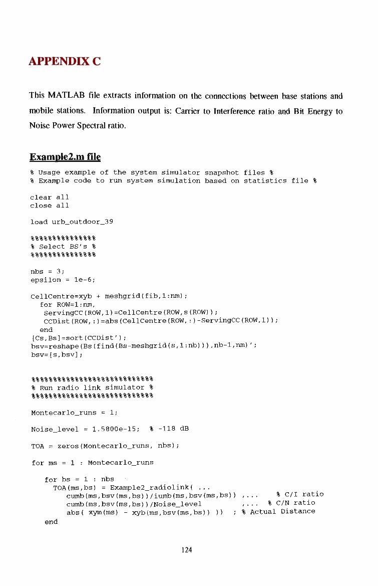
APPENDIX C
This M A T L A B file extracts information on the connections between base stations and
mobile stations. Information output is: Carrier to Interference ratio and Bit Energy to
Noise Power Spectral ratio.
Example2.m file
% Usage example of the system simulator snapshot files % % Example code to run system simulation based on statistics file %
clear all close all
load urb_outdoor_39
%%%%%%%%%%%%%%%
% Select BS's % %%%%%%%%%%%%%%%
nbs = 3; epsilon = le-6;
CellCentre=xyb + meshgrid(fib,1:nm); for ROW=l:nm, ServingCC(ROW,1)=CellCentre(ROW,s(ROW)); CCDist(ROW,:)=abs(CellCentre(ROW,:)-ServingCC(ROW,1)); end
[Cs,Bs]=sort(CCDist'); bsv=reshape(Bs(find(Bs-meshgrid(s,l:nb))),nb-l,nm)' ; bsv=[s,bsv];
%%%%%%%%%%%%%%%%%%%%%%%%%%%%
% Run radio link simulator % %%%%%%%%%%%%%%%%%%%%%%%%%%%%
Montecarlo_runs = 1;
Noise_level = 1.5800e-15; % -118 dB
TOA = zeros(Montecarlo_runs, nbs);
for ms = 1 : Montecarlo_runs
for bs = 1 : nbs TOA(ms,bs) = Example2_radiolink( ...
cumb(ms,bsv(ms,bs))/iumb(ms,bsv(ms,bs)) ,... % C/I ratio cumb(ms,bsv(ms,bs))/Noise_level ,... % C/N ratio abs( xym(ms) - xyb(ms,bsv(ms,bs)) )) ; % Actual Distance
end
124

end % *** <eof> *** %
125

APPENDIX D
This M A T L A B file outputs the location of the estimated mobile station.
location.m file
% Matlab file that sovles position location of mobile. % Inputs are base station coordinates.
%Enter here BS coordinates
Xbsl = 0; Ybsl = 0;
Xbs2 = 1500; Ybs2 = -2.27e-13;
% Enter distances from BS's to MS
dl = 300; % MS to BS1 d2 = 12 60; % MS to BS2
% Solve equation 1, which BS1.
%((Xm-Xbsl)MXm-Xbsl)) + ((Ym-Ybsl) * (Ym-Ybsl)) = (dl*dl) ;
%(Xm*Xm)-(Xbsl*Xm)-(Xbsl*Xm)+(Xbsl*Xbsl) + (Ym*Ym)-(Ybsl*Ym)-(Ybsl*Ym)+(Ybsl*Ybsl) = (dl*dl);
a=Xbsl*Xbsl; b=Ybsl*Ybsl; c=dl*dl;
% Now equation 1 is: %(Xm*Xm)-(Xbsl*Xm)-(Xbsl*Xm)+a + (Ym*Ym)-(Ybsl*Ym)-(Ybsl*Ym)+b = c;
%(Xm*Xm)-((Xbsl-Xbsl)*Xm))+a + (Ym*Ym)-((Ybsl-Ybsl)*Ym))+b = c;
%(Xm*Xm)-((Xbsl-Xbsl)*Xm))+(Ym*Ym)-((Ybsl-Ybsl)*Ym))+a+b-c = 0;
d=a+b-c;
% Now equation 1 is:
%(Xm*Xm)-((Xbsl-Xbsl)*Xm))+(Ym*Ym)-((Ybsl-Ybsl)*Ym))+d = 0;
z=Xbsl-Xbsl; y=Ybsl-Ybsl;
% Therefore equation 1 is:
126
%(Xm*Xm)-(z*Xm) ) + (Ym*Ym)-(y*Ym) )+d = 0;
% Solve equation 2, which is BS2.
%((Xm-Xbs2)*(Xm-Xbs2)) + ((Ym-Ybs2)*(Ym-Ybs2)) = (d2*d2);
%(Xm*Xm)-(Xbs2*Xm)-(Xbs2*Xm) + (Xbs2*Xbs2) + (Ym*Ym)-(Ybs2*Ym)-(Ybs2*Ym)+(Ybs2*Ybs2) = (d2*d2);
e=Xbs2*Xbs2; f=Ybs2*Ybs2; g=d2*d2;
% Now equation 2 is: %(Xm*Xm)-(Xbs2*Xm)-(Xbs2*Xm)+e + (Ym*Ym) - (Ybs2*Ym) - (Ybs2*Ym)+f = g;
%(Xm*Xm)-((Xbs2-Xbs2)*Xm))+e + (Ym*Ym) - ((Ybs2-Ybs2) *Ym) )+f = g;
%(Xm*Xm)-((Xbs2-Xbs2)*Xm)) + (Ym*Ym)-((Ybs2-Ybs2)*Ym))+e+f-g = 0;
h=e+f-g;
% Now equation 2 is:
%(Xm*Xm)-( (Xbs2-Xbs2)*Xm) ) + (Ym*Ym)-( (Ybs2-Ybs2) *Ym) )+h = 0;
k=Xbs2-Xbs2; j=Ybs2-Ybs2;
% Therefore equation 2 is:
%(Xm*Xm)-(k*Xm))+(Ym*Ym)-(j*Ym))+h = 0;
% Now use simultanious equations. Eql-Eq2.
%((Xm*Xm)-(z*Xm)) + (Ym*Ym)-(y*Ym))+d) - ( (Xm*Xm) - (k*Xm)) + (Ym*Ym)-(j*Ym))+h) = 0;
%((-z+k)*Xm) + ((-y+j)*Ym) + (d-h) = 0;
n=-z+k; m=-y+j; p=d-h;
% Therefore
%(n*Xm) + (m*Ym) + p = 0;
%(n*Xm) = -(m*Ym)-p;
% So Xm is:
127

%Xm = -((m/n)*Ym) + (p/n);
al=m/n; a2=p/n;
%Xm = -(al*Ym) + a2;
% Now sub this equation of Xm in equation 2.
%(Xm*Xm)-(k*Xm))+(Ym*Ym)-(j*Ym))+h = 0; % this is equation 2.
%((-al*Ym + a2)*(-al*Ym + a2)) - (k*(-al*Ym + a2)) + (Ym*Ym) - (j*Ym) + h = 0;
%(((al*al)*Ym*Ym)-(al*a2*Ym)-(a2*al*Ym)+(al*a2)) - (-k*al*Ym + k*a2) + (Ym*Ym) - (j*Ym) + h = 0;
sl=al*al; s2=al*a2; s3=k*al; s4=k*a2;
%<sl*Ym*Ym - s2*Ym -s2*Ym + s2) - (-s3*Ym + s4) + (l*Ym*Ym) - (j*Ym) + h = 0;
%sl*Ym*Ym - (s2+s2)*Ym + s2 + s3*Ym - s4 + l*Ym*Ym - j*Ym + h = 0;
ql=s2+s2;
%sl*Ym*Ym - ql*Ym + s2 + s3*Ym - s4 + l*Ym*Ym - j*Ym + h = 0;
%(sl+l)*Ym*Ym - (ql+s3-j)*Ym + (s2-s4+h) = 0;
tl=sl+l; t2=ql+s3-j; t3=s2-s4+h;
% tl*Ym*Ym - t2*Ym + t3 = 0;
% Quadratic formula:
Yml = (-t2 + (sqrt(t2*t2 - 4*tl*t3)) / (2*tl));
Ym2 = (-t2 - (sqrt(t2*t2 - 4*tl*t3)) / (2*tl));
% end of file %
128