$fwlydwh - altair engineering
TRANSCRIPT

6ALTAIR
Altair Activate®
Altair Activate® 2021 Extended DefinitionsCopyright © 2021 Altair Engineering, Inc. All rights reserved.

Intellectual Property Rights Notice: Copyrights, Trademarks, Trade Secrets, Patents & Third-Party Software Licenses Altair Engineering Inc. Copyright © 1986-2020. All Rights Reserved. Copyrights in the below are held by Altair Engineering, Inc., except where otherwise explicitly stated.
Special Notice: Pre-release versions of Altair software are provided ‘as is’, without warranty of any kind. Usage of pre-release versions is strictly limited to non-production purposes.
Altair HyperWorks™ - The Platform for Innovation™ Altair AcuConsole™ ©2006-2020 Altair AcuSolve™ ©1997-2020 Altair Activate® ©1989-2020 (formerly solidThinking Activate®) Altair Compose® ©2007-2020 (formerly solidThinking Compose®) Altair ConnectMe™ ©2014-2020 Altair EDEM © 2005-2020 DEM Solutions Ltd, © 2019-2020 Altair Engineering, Inc. Altair ElectroFlo™ ©1992-2020 Altair Embed® ©1989-2020 (formerly solidThinking Embed®)
o Altair Embed SE ©1989-2020 (formerly solidThinking Embed® SE) o Altair Embed / Digital Power Designer ©2012-2020 o Altair Embed Viewer ©1996-2020
Altair ESAComp™ ©1992-2020 Altair Feko™ ©1999-2014 Altair Development S.A. (Pty) Ltd., ©2014-2020 Altair Engineering Inc. Altair Flux™ ©1983-2020 Altair FluxMotor™ ©2017-2020 Altair HyperCrash™ ©2001-2020 Altair HyperGraph™ ©1995-2020 Altair HyperLife™ ©1990-2020 Altair HyperMesh™ ©1990-2020 Altair HyperStudy™ ©1999-2020 Altair HyperView™ ©1999-2020 Altair HyperXtrude™ ©1999-2020 Altair Inspire™ ©2009-2020 including Altair Inspire Motion, Altair Inspire Structures, and Altair Inspire Print3D Altair Inspire Cast ©2011-2020 (formerly Click2Cast®) Altair Inspire Extrude Metal ©1996-2020 (formerly Click2Extrude® - Metal) Altair Inspire Extrude Polymer ©1996-2020 (formerly Click2Extrude® - Polymer) Altair Inspire Form ©1998-2020 (formerly Click2Form®) Altair Inspire Friction Stir Welding ©1996-2020 Altair Inspire Mold ©2009-2020 Altair Inspire PolyFoam ©2009-2020 Altair Inspire Render ©1993-2016 Solid Iris Technologies Software Development One PLLC, © 2016-2020 Altair Engineering Inc (formerly Thea Studio) Altair Inspire Studio ©1993-2020 (formerly ‘Evolve’) Altair Manufacturing Solver™ © 2011-2020 Altair MotionSolve™ ©2002-2020 Altair MotionView™ ©1993-2020 Altair Multiscale Designer™ ©2011-2020 Altair nanoFluidX™ ©2013-2018 Fluidyna GmbH, © 2018-2020 Altair Engineering Inc. Altair newFASANT ©2010-2020 Altair OptiStruct™ ©1996-2020 Altair PollEx ©2003-2020 Altair Radioss™ ©1986-2020
Altair Activate 2021
Proprietary Information of Altair Engineering Inc.
Extended Definitions 2

Altair Seam™ © 1985-2019 Cambridge Collaborative, Inc., © 2019-2020 Altair Engineering Inc. Altair SimLab™ ©2004-2020 Altair SimSolid™ ©2015-2020 Altair ultraFluidX™ ©2010-2018 Fluidyna GmbH, © 2018-2020 Altair Engineering Inc. Altair Virtual Wind Tunnel™ ©2012-2020 Altair WinProp™ ©2000-2020 Altair WRAP ©1998-2020 WRAP International AB, © 2020 Altair Engineering AB Altair Packaged Solution Offerings (PSOs) Altair Automated Reporting Director™ ©2008-2020 Altair GeoMechanics Director™ ©2011-2020 Altair Impact Simulation Director™ ©2010-2020 Altair Model Mesher Director™ ©2010-2020 Altair NVH Director™ ©2010-2020 Altair Squeak and Rattle Director™ ©2012-2020 Altair Virtual Gauge Director™ ©2012-2020 Altair Weight Analytics™ ©2013-2020 Altair Weld Certification Director™ ©2014-2020 Altair Multi-Disciplinary Optimization Director™ ©2012-2020 Altair PBS Works™ - Accelerating Innovation in the Cloud™ Altair® PBS Professional® ©1994-2020 Altair Control™ ©2008-2020; (formerly PBS Control) Altair Access™ ©2008-2020; (formerly PBS Access) Altair Accelerator™ ©1995-2020; (formerly NetworkComputer) Altair Accelerator™ Plus ©1995-2020; (formerly WorkloadXelerator) Altair FlowTracer™ ©1995-2020; (formerly FlowTracer) Altair Allocator™ ©1995-2020; (formerly LicenseAllocator) Altair Monitor™ ©1995-2020; (formerly LicenseMonitor) Altair Hero™ ©1995-2020; (formerly HERO) Altair Software Asset Optimization (SAO) ©2007-2020 Note: Compute Manager™ ©2012-2017 is now part of Altair Access Display Manager™ ©2013-2017 is now part of Altair Access PBS Application Services™ ©2008-2017 is now part of Altair Access PBS Analytics™ ©2008-2017 is now part of Altair Control PBS Desktop™ ©2008-2012 is now part of Altair Access, specifically Altair Access desktop, which also has Altair Access web and Altair Access mobile e-Compute™ ©2000-2010 was replaced by “Compute Manager” which is now Altair Access Altair KnowledgeWorks™ Altair Knowledge Studio® © 1994-2020 Angoss Software Corporation, © 2020 Altair Engineering, Inc. Altair Knowledge Studio for Apache Spark © 1994-2020 Angoss Software Corporation, © 2020 Altair Engineering, Inc. Altair Knowledge Seeker™ © 1994-2020 Angoss Software Corporation, © 2020 Altair Engineering, Inc. Altair Knowledge Hub™ © 2017-2020 Datawatch Corporation, © 2020 Altair Engineering, Inc. Altair Monarch™ © 1996-2020 Datawatch Corporation, © 2020 Altair Engineering, Inc. Altair Monarch Server © 1996-2020 Datawatch Corporation, © 2020 Altair Engineering, Inc. Altair Panopticon™ © 2004-2020 Datawatch Corporation, © 2020 Altair Engineering, Inc. Altair SmartWorks™ Altair SmartCore™ © 2011-2020 Altair SmartEdge™ © 2011-2020
3 Extended Definitions
Proprietary Information of Altair Engineering Inc.
Altair Activate 2021

Altair SmartSight™ © 2011-2020 Altair One™ ©1994-2020 Altair intellectual property rights are protected under U.S. and international laws and treaties. Additionally, Altair software may be protected by patents. All other marks are the property of their respective owners. ALTAIR ENGINEERING INC. Proprietary and Confidential. Contains Trade Secret Information. Not for use or disclosure outside of Altair and its licensed clients. Information contained in Altair software shall not be decompiled, disassembled, “unlocked”, reverse translated, reverse engineered, or publicly displayed or publicly performed in any manner. Usage of the software is only as explicitly permitted in the end user software license agreement. Copyright notice does not imply publication. Third-party software licenses AcuConsole contains material licensed from Intelligent Light (www.ilight.com) and used by permission. Software Security Measures: Altair Engineering Inc. and its subsidiaries and affiliates reserve the right to embed software security mechanisms in the Software for the purpose of detecting the installation and/or use of illegal copies of the Software. The Software may collect and transmit non-proprietary data about those illegal copies. Data collected will not include any customer data created by or used in connection with the Software and will not be provided to any third party, except as may be required by law or legal process or to enforce our rights with respect to the use of any illegal copies of the Software. By using the Software, each user consents to such detection and collection of data, as well as its transmission and use if an illegal copy of the Software is detected. No steps may be taken to avoid or detect the purpose of any such security mechanisms.
Altair Activate 2021
Proprietary Information of Altair Engineering Inc.
Extended Definitions 4

Contents
1 Activation signals in Altair Activate 131.1 Introduction . . . . . . . . . . . . . . . . . . . . . . . . . . . . . . . . . . . . . . . . . . 13
1.1.1 Simple queue . . . . . . . . . . . . . . . . . . . . . . . . . . . . . . . . . . . . . 151.1.2 Traffic simulation . . . . . . . . . . . . . . . . . . . . . . . . . . . . . . . . . . . . 181.1.3 Re-initialization of continuous-time state . . . . . . . . . . . . . . . . . . . . . . . 211.1.4 Communication delay . . . . . . . . . . . . . . . . . . . . . . . . . . . . . . . . . 22
1.2 Types of activation signals . . . . . . . . . . . . . . . . . . . . . . . . . . . . . . . . . . 281.2.1 Programmed events . . . . . . . . . . . . . . . . . . . . . . . . . . . . . . . . . . 281.2.2 Zero-crossing events . . . . . . . . . . . . . . . . . . . . . . . . . . . . . . . . . 281.2.3 Continuous-time activation signal . . . . . . . . . . . . . . . . . . . . . . . . . . . 281.2.4 Initial-time activation signal . . . . . . . . . . . . . . . . . . . . . . . . . . . . . . 291.2.5 Periodic activation signals . . . . . . . . . . . . . . . . . . . . . . . . . . . . . . . 29
1.3 Activation inheritance . . . . . . . . . . . . . . . . . . . . . . . . . . . . . . . . . . . . . 301.4 Synchronous vs. asynchronous activations . . . . . . . . . . . . . . . . . . . . . . . . . 31
1.4.1 Conditional blocks . . . . . . . . . . . . . . . . . . . . . . . . . . . . . . . . . . . 321.4.2 Sample and Resample Clock blocks . . . . . . . . . . . . . . . . . . . . . . . . . 32
2 Altair Activate Matrix Expression Block 372.1 Introduction . . . . . . . . . . . . . . . . . . . . . . . . . . . . . . . . . . . . . . . . . . 372.2 Examples . . . . . . . . . . . . . . . . . . . . . . . . . . . . . . . . . . . . . . . . . . . 38
2.2.1 Basic operators and functions . . . . . . . . . . . . . . . . . . . . . . . . . . . . 382.2.2 Matrix construction, extraction and assignment . . . . . . . . . . . . . . . . . . . 392.2.3 Use of OML functions . . . . . . . . . . . . . . . . . . . . . . . . . . . . . . . . . 40
2.3 Parser . . . . . . . . . . . . . . . . . . . . . . . . . . . . . . . . . . . . . . . . . . . . . 412.4 Limitations . . . . . . . . . . . . . . . . . . . . . . . . . . . . . . . . . . . . . . . . . . . 42
2.4.1 Fixed-sized matrix principle . . . . . . . . . . . . . . . . . . . . . . . . . . . . . . 422.4.2 All the branches of conditional expressions evaluated . . . . . . . . . . . . . . . . 422.4.3 No support for logical type . . . . . . . . . . . . . . . . . . . . . . . . . . . . . . 42
2.5 Data types . . . . . . . . . . . . . . . . . . . . . . . . . . . . . . . . . . . . . . . . . . . 432.5.1 Supported data type . . . . . . . . . . . . . . . . . . . . . . . . . . . . . . . . . . 432.5.2 Unsupported data types . . . . . . . . . . . . . . . . . . . . . . . . . . . . . . . . 432.5.3 Data coding . . . . . . . . . . . . . . . . . . . . . . . . . . . . . . . . . . . . . . 43
2.6 Supported operators . . . . . . . . . . . . . . . . . . . . . . . . . . . . . . . . . . . . . 432.6.1 Arithmetic operators . . . . . . . . . . . . . . . . . . . . . . . . . . . . . . . . . . 432.6.2 Matrix construction and structuring . . . . . . . . . . . . . . . . . . . . . . . . . . 442.6.3 Relational and logical operators . . . . . . . . . . . . . . . . . . . . . . . . . . . 452.6.4 Conditional operators . . . . . . . . . . . . . . . . . . . . . . . . . . . . . . . . . 46
5 Extended Definitions
Proprietary Information of Altair Engineering Inc.
Altair Activate 2021

2.7 Supported functions . . . . . . . . . . . . . . . . . . . . . . . . . . . . . . . . . . . . . . 462.7.1 Supported functions . . . . . . . . . . . . . . . . . . . . . . . . . . . . . . . . . . 472.7.2 Using OML functions . . . . . . . . . . . . . . . . . . . . . . . . . . . . . . . . . 48
3 C and OML Custom Blocks in Altair Activate 493.1 Activate block simulation function . . . . . . . . . . . . . . . . . . . . . . . . . . . . . . 503.2 Custom block parameter GUI . . . . . . . . . . . . . . . . . . . . . . . . . . . . . . . . . 503.3 Examples . . . . . . . . . . . . . . . . . . . . . . . . . . . . . . . . . . . . . . . . . . . 52
3.3.1 Median block . . . . . . . . . . . . . . . . . . . . . . . . . . . . . . . . . . . . . . 523.3.2 Variable discrete delay . . . . . . . . . . . . . . . . . . . . . . . . . . . . . . . . 563.3.3 Fluid flow . . . . . . . . . . . . . . . . . . . . . . . . . . . . . . . . . . . . . . . . 593.3.4 Simplified explicit automaton block . . . . . . . . . . . . . . . . . . . . . . . . . . 62
3.4 Non-inlined simulation functions . . . . . . . . . . . . . . . . . . . . . . . . . . . . . . . 67
4 Simulation restarts: implementing iterations 714.1 Nonlinear solver block . . . . . . . . . . . . . . . . . . . . . . . . . . . . . . . . . . . . . 72
4.1.1 A reverse-communication solver . . . . . . . . . . . . . . . . . . . . . . . . . . . 724.1.2 Activate block implementation . . . . . . . . . . . . . . . . . . . . . . . . . . . . 754.1.3 Examples . . . . . . . . . . . . . . . . . . . . . . . . . . . . . . . . . . . . . . . 764.1.4 Solving nonlinear system without a specific block . . . . . . . . . . . . . . . . . . 80
4.2 Repeating activations . . . . . . . . . . . . . . . . . . . . . . . . . . . . . . . . . . . . . 834.2.1 Problem setup . . . . . . . . . . . . . . . . . . . . . . . . . . . . . . . . . . . . . 844.2.2 System equations . . . . . . . . . . . . . . . . . . . . . . . . . . . . . . . . . . . 844.2.3 Implementation in Activate . . . . . . . . . . . . . . . . . . . . . . . . . . . . . . 85
5 Example: Implementation of an Extended Kalman Filter in Activate 895.1 Activate model . . . . . . . . . . . . . . . . . . . . . . . . . . . . . . . . . . . . . . . . 905.2 EKF model . . . . . . . . . . . . . . . . . . . . . . . . . . . . . . . . . . . . . . . . . . . 915.3 Covariance prediction . . . . . . . . . . . . . . . . . . . . . . . . . . . . . . . . . . . . . 925.4 State update . . . . . . . . . . . . . . . . . . . . . . . . . . . . . . . . . . . . . . . . . . 935.5 Simulation . . . . . . . . . . . . . . . . . . . . . . . . . . . . . . . . . . . . . . . . . . . 94
6 Optimization 996.1 Use of Optimization block in Activate . . . . . . . . . . . . . . . . . . . . . . . . . . . . 996.2 Example . . . . . . . . . . . . . . . . . . . . . . . . . . . . . . . . . . . . . . . . . . . . 1006.3 GetFromeBase and AddToBase OML functions . . . . . . . . . . . . . . . . . . . . . 1076.4 Script based optimization . . . . . . . . . . . . . . . . . . . . . . . . . . . . . . . . . . . 112
6.4.1 Direct scripting of optimization code in OML . . . . . . . . . . . . . . . . . . . . . 1126.4.2 Example . . . . . . . . . . . . . . . . . . . . . . . . . . . . . . . . . . . . . . . . 113
6.5 Activate Graphical optimization tool . . . . . . . . . . . . . . . . . . . . . . . . . . . . . 1176.5.1 Example . . . . . . . . . . . . . . . . . . . . . . . . . . . . . . . . . . . . . . . . 118
6.6 Max-min/Min-max optimization problems . . . . . . . . . . . . . . . . . . . . . . . . . . 120
7 Linearization 1257.1 Linearization function . . . . . . . . . . . . . . . . . . . . . . . . . . . . . . . . . . . . . 125
7.1.1 Example: inverted pendulum . . . . . . . . . . . . . . . . . . . . . . . . . . . . . 1267.1.2 Example: Cart on a beam . . . . . . . . . . . . . . . . . . . . . . . . . . . . . . . 131
7.2 Computation of the equilibrium point . . . . . . . . . . . . . . . . . . . . . . . . . . . . . 1367.2.1 Use of infinite steady-state gain controller . . . . . . . . . . . . . . . . . . . . . . 138
Altair Activate 2021
Proprietary Information of Altair Engineering Inc.
Extended Definitions 6

7.2.2 Equilibrium point for the inverted pendulum example . . . . . . . . . . . . . . . . 1407.2.3 3D model of a spacecraft for take off and landing control . . . . . . . . . . . . . . 145
7.3 Modeling in Activate . . . . . . . . . . . . . . . . . . . . . . . . . . . . . . . . . . . . . 1477.4 State feedback control . . . . . . . . . . . . . . . . . . . . . . . . . . . . . . . . . . . . 148
8 Altair Activate Libraries 1558.1 Library structure . . . . . . . . . . . . . . . . . . . . . . . . . . . . . . . . . . . . . . . . 1558.2 Block structure . . . . . . . . . . . . . . . . . . . . . . . . . . . . . . . . . . . . . . . . . 1578.3 Palette . . . . . . . . . . . . . . . . . . . . . . . . . . . . . . . . . . . . . . . . . . . . . 1578.4 Library creation . . . . . . . . . . . . . . . . . . . . . . . . . . . . . . . . . . . . . . . . 158
8.4.1 Library Manager . . . . . . . . . . . . . . . . . . . . . . . . . . . . . . . . . . . . 1588.4.2 OML functions . . . . . . . . . . . . . . . . . . . . . . . . . . . . . . . . . . . . . 160
9 Altair Activate blocks 1639.1 Block simulation function . . . . . . . . . . . . . . . . . . . . . . . . . . . . . . . . . . . 163
9.1.1 Simulation function implementation . . . . . . . . . . . . . . . . . . . . . . . . . . 1659.1.2 Examples . . . . . . . . . . . . . . . . . . . . . . . . . . . . . . . . . . . . . . . 1719.1.3 Macros for accessing the block structure . . . . . . . . . . . . . . . . . . . . . . . 1849.1.4 Macros for accessing the simulator structure . . . . . . . . . . . . . . . . . . . . 189
9.2 Block builder . . . . . . . . . . . . . . . . . . . . . . . . . . . . . . . . . . . . . . . . . . 1919.2.1 Atom: Basic block . . . . . . . . . . . . . . . . . . . . . . . . . . . . . . . . . . . 1929.2.2 Atom: Programmable Super Block . . . . . . . . . . . . . . . . . . . . . . . . . . 193
10 Activate hybrid simulator and its interface with numerical solvers 20310.1 Introduction . . . . . . . . . . . . . . . . . . . . . . . . . . . . . . . . . . . . . . . . . . 20310.2 Simulation of an hybrid model in Activate . . . . . . . . . . . . . . . . . . . . . . . . . . 20610.3 Numerical solver classifications and characteristics . . . . . . . . . . . . . . . . . . . . . 210
10.3.1 Stiff vs. non-stiff ODE . . . . . . . . . . . . . . . . . . . . . . . . . . . . . . . . . 21110.3.2 Explicit vs. Implicit Solvers . . . . . . . . . . . . . . . . . . . . . . . . . . . . . . 21110.3.3 Fixed-step vs. variable-step solvers . . . . . . . . . . . . . . . . . . . . . . . . . 21210.3.4 Analytical vs. numerical Jacobian matrix . . . . . . . . . . . . . . . . . . . . . . . 21210.3.5 Single-step vs. multi-step solvers . . . . . . . . . . . . . . . . . . . . . . . . . . . 21310.3.6 ODE vs. DAE solver . . . . . . . . . . . . . . . . . . . . . . . . . . . . . . . . . . 213
10.4 Numerical Solver interface with the simulator . . . . . . . . . . . . . . . . . . . . . . . . 21410.4.1 Forward looking in time (stopping time) . . . . . . . . . . . . . . . . . . . . . . . 21410.4.2 Zero-crossing and event-detection . . . . . . . . . . . . . . . . . . . . . . . . . . 21410.4.3 Cold-start versus hot-start of the solver . . . . . . . . . . . . . . . . . . . . . . . 21510.4.4 Absolute and relative error tolerances . . . . . . . . . . . . . . . . . . . . . . . . 21510.4.5 Maximum, minimum, and initial step-size . . . . . . . . . . . . . . . . . . . . . . 21610.4.6 Fixed-step solver interface with the simulator . . . . . . . . . . . . . . . . . . . . 21610.4.7 Numerical solvers available in Activate . . . . . . . . . . . . . . . . . . . . . . . 216
11 Physical component modeling in Altair Activate 22311.1 Introduction . . . . . . . . . . . . . . . . . . . . . . . . . . . . . . . . . . . . . . . . . . 22311.2 Causal vs. acausal modeling . . . . . . . . . . . . . . . . . . . . . . . . . . . . . . . . . 22311.3 Modelica: a standard in component level modeling . . . . . . . . . . . . . . . . . . . . . 225
11.3.1 Example: modeling a DC motor . . . . . . . . . . . . . . . . . . . . . . . . . . . 22711.4 Implementation in Activate . . . . . . . . . . . . . . . . . . . . . . . . . . . . . . . . . . 228
7 Extended Definitions
Proprietary Information of Altair Engineering Inc.
Altair Activate 2021

11.5 Modelica custom block . . . . . . . . . . . . . . . . . . . . . . . . . . . . . . . . . . . . 230
12 FMI (Functional Mock-up Interface) 23512.1 Introduction . . . . . . . . . . . . . . . . . . . . . . . . . . . . . . . . . . . . . . . . . . 235
12.1.1 FMI interface types . . . . . . . . . . . . . . . . . . . . . . . . . . . . . . . . . . 23612.1.2 Advantages of using FMI in industry . . . . . . . . . . . . . . . . . . . . . . . . . 236
12.2 Internal structure of an FMU . . . . . . . . . . . . . . . . . . . . . . . . . . . . . . . . . 23812.3 FMI for Model Exchange (ME) . . . . . . . . . . . . . . . . . . . . . . . . . . . . . . . . 23912.4 FMI for Co-Simulation (CS) . . . . . . . . . . . . . . . . . . . . . . . . . . . . . . . . . . 241
12.4.1 Co-simulation algorithms . . . . . . . . . . . . . . . . . . . . . . . . . . . . . . . 24212.4.2 Advanced: FMI import preserving full output/input dependency property . . . . . 244
12.5 FMI Import in Activate . . . . . . . . . . . . . . . . . . . . . . . . . . . . . . . . . . . . 24512.5.1 Direct dependency vector for inputs (Feedthrough) . . . . . . . . . . . . . . . . . 24612.5.2 Advanced tab . . . . . . . . . . . . . . . . . . . . . . . . . . . . . . . . . . . . . 24612.5.3 Reporting tab . . . . . . . . . . . . . . . . . . . . . . . . . . . . . . . . . . . . . 24812.5.4 ModelExchange tab . . . . . . . . . . . . . . . . . . . . . . . . . . . . . . . . . . 24912.5.5 CoSimulation tab . . . . . . . . . . . . . . . . . . . . . . . . . . . . . . . . . . . 25012.5.6 Example . . . . . . . . . . . . . . . . . . . . . . . . . . . . . . . . . . . . . . . . 251
12.6 FMI export in Activate . . . . . . . . . . . . . . . . . . . . . . . . . . . . . . . . . . . . 25112.6.1 Nested FMU . . . . . . . . . . . . . . . . . . . . . . . . . . . . . . . . . . . . . . 25212.6.2 Exporting Modelica . . . . . . . . . . . . . . . . . . . . . . . . . . . . . . . . . . 25212.6.3 Shortcomings . . . . . . . . . . . . . . . . . . . . . . . . . . . . . . . . . . . . . 25312.6.4 Requirements . . . . . . . . . . . . . . . . . . . . . . . . . . . . . . . . . . . . . 25312.6.5 Example . . . . . . . . . . . . . . . . . . . . . . . . . . . . . . . . . . . . . . . . 254
12.7 Advanced user topics: . . . . . . . . . . . . . . . . . . . . . . . . . . . . . . . . . . . . . 255
13 Co-Simulation with Multi-body Simulation 26313.1 Introduction . . . . . . . . . . . . . . . . . . . . . . . . . . . . . . . . . . . . . . . . . . 26313.2 Co-Simulation with MBS . . . . . . . . . . . . . . . . . . . . . . . . . . . . . . . . . . . 263
13.2.1 Under the hood . . . . . . . . . . . . . . . . . . . . . . . . . . . . . . . . . . . . 26613.3 MSplant block parameters . . . . . . . . . . . . . . . . . . . . . . . . . . . . . . . . . . 26813.4 Example: Pendulum Swing-Up . . . . . . . . . . . . . . . . . . . . . . . . . . . . . . . . 269
14 CoSimulation with Electromagnetic and Thermal Models 27714.1 Introduction on Flux . . . . . . . . . . . . . . . . . . . . . . . . . . . . . . . . . . . . . . 27714.2 CoSimulation with Flux . . . . . . . . . . . . . . . . . . . . . . . . . . . . . . . . . . . . 27714.3 Flux block parameters . . . . . . . . . . . . . . . . . . . . . . . . . . . . . . . . . . . . 281
14.3.1 Parameters tab . . . . . . . . . . . . . . . . . . . . . . . . . . . . . . . . . . . . 28114.3.2 Flux Activation tab . . . . . . . . . . . . . . . . . . . . . . . . . . . . . . . . . . . 28214.3.3 Reporting tab . . . . . . . . . . . . . . . . . . . . . . . . . . . . . . . . . . . . . 28314.3.4 Advanced tab . . . . . . . . . . . . . . . . . . . . . . . . . . . . . . . . . . . . . 284
14.4 Example: Brushless AC embedded permanent magnet motor . . . . . . . . . . . . . . . 28514.5 Example: Externally activated block . . . . . . . . . . . . . . . . . . . . . . . . . . . . . 285
15 HyperSpice in Altair Activate 28915.1 Introduction . . . . . . . . . . . . . . . . . . . . . . . . . . . . . . . . . . . . . . . . . . 289
15.1.1 What is exactly SPICE ? . . . . . . . . . . . . . . . . . . . . . . . . . . . . . . . 28915.1.2 Why using SPICE ? . . . . . . . . . . . . . . . . . . . . . . . . . . . . . . . . . . 289
Altair Activate 2021
Proprietary Information of Altair Engineering Inc.
Extended Definitions 8

15.2 HyperSpiceTM . . . . . . . . . . . . . . . . . . . . . . . . . . . . . . . . . . . . . . . . . 28915.3 Spice Language . . . . . . . . . . . . . . . . . . . . . . . . . . . . . . . . . . . . . . . . 290
15.3.1 Units . . . . . . . . . . . . . . . . . . . . . . . . . . . . . . . . . . . . . . . . . . 29015.3.2 Comments . . . . . . . . . . . . . . . . . . . . . . . . . . . . . . . . . . . . . . . 29115.3.3 Resistor . . . . . . . . . . . . . . . . . . . . . . . . . . . . . . . . . . . . . . . . 29115.3.4 Capacitor . . . . . . . . . . . . . . . . . . . . . . . . . . . . . . . . . . . . . . . 29215.3.5 Inductor . . . . . . . . . . . . . . . . . . . . . . . . . . . . . . . . . . . . . . . . 29315.3.6 Mutual Inductors . . . . . . . . . . . . . . . . . . . . . . . . . . . . . . . . . . . . 29415.3.7 Mosfet . . . . . . . . . . . . . . . . . . . . . . . . . . . . . . . . . . . . . . . . . 29415.3.8 BJT . . . . . . . . . . . . . . . . . . . . . . . . . . . . . . . . . . . . . . . . . . . 29815.3.9 JFET . . . . . . . . . . . . . . . . . . . . . . . . . . . . . . . . . . . . . . . . . . 30015.3.10Switches . . . . . . . . . . . . . . . . . . . . . . . . . . . . . . . . . . . . . . . . 30115.3.11Transmission Lines . . . . . . . . . . . . . . . . . . . . . . . . . . . . . . . . . . 30315.3.12Diode . . . . . . . . . . . . . . . . . . . . . . . . . . . . . . . . . . . . . . . . . . 30615.3.13S-Parameter blocks . . . . . . . . . . . . . . . . . . . . . . . . . . . . . . . . . . 30715.3.14Linear Dependent Sources . . . . . . . . . . . . . . . . . . . . . . . . . . . . . . 30815.3.15Linear Independent Sources . . . . . . . . . . . . . . . . . . . . . . . . . . . . . 30915.3.16Hierarchy declaration . . . . . . . . . . . . . . . . . . . . . . . . . . . . . . . . . 31315.3.17Parameters . . . . . . . . . . . . . . . . . . . . . . . . . . . . . . . . . . . . . . 31415.3.18S-Parameter extraction . . . . . . . . . . . . . . . . . . . . . . . . . . . . . . . . 31415.3.19Options . . . . . . . . . . . . . . . . . . . . . . . . . . . . . . . . . . . . . . . . . 315
15.4 Known Issues . . . . . . . . . . . . . . . . . . . . . . . . . . . . . . . . . . . . . . . . . 31615.5 SpiceCustomBlock . . . . . . . . . . . . . . . . . . . . . . . . . . . . . . . . . . . . . . 317
16 Hybrid Automata in Altair Activate 32516.1 Abstract . . . . . . . . . . . . . . . . . . . . . . . . . . . . . . . . . . . . . . . . . . . . 32516.2 Introduction . . . . . . . . . . . . . . . . . . . . . . . . . . . . . . . . . . . . . . . . . . 32516.3 Automaton Block . . . . . . . . . . . . . . . . . . . . . . . . . . . . . . . . . . . . . . . 327
16.3.1 Example 1: Pendulum Swing Up . . . . . . . . . . . . . . . . . . . . . . . . . . . 32916.3.2 Example 2: DC/DC Buck Converter . . . . . . . . . . . . . . . . . . . . . . . . . 33116.3.3 Example 3: Sticky balls . . . . . . . . . . . . . . . . . . . . . . . . . . . . . . . . 335
16.4 conclusion . . . . . . . . . . . . . . . . . . . . . . . . . . . . . . . . . . . . . . . . . . . 339
17 Interpolation and extrapolation methods in Activate 34317.1 Introduction . . . . . . . . . . . . . . . . . . . . . . . . . . . . . . . . . . . . . . . . . . 34317.2 Interpolation methods . . . . . . . . . . . . . . . . . . . . . . . . . . . . . . . . . . . . . 34417.3 Extrapolation methods . . . . . . . . . . . . . . . . . . . . . . . . . . . . . . . . . . . . 349
17.3.1 Application - Behavior in blocks . . . . . . . . . . . . . . . . . . . . . . . . . . . . 352
18 SignalOut and SignalIn blocks in Altair Activate 35518.1 Introduction . . . . . . . . . . . . . . . . . . . . . . . . . . . . . . . . . . . . . . . . . . 35518.2 Activation information inside a signal object . . . . . . . . . . . . . . . . . . . . . . . . . 35618.3 SignalOut block . . . . . . . . . . . . . . . . . . . . . . . . . . . . . . . . . . . . . . . . 35718.4 SignalIn block . . . . . . . . . . . . . . . . . . . . . . . . . . . . . . . . . . . . . . . . . 359
19 Animation 36119.1 Anim2D block . . . . . . . . . . . . . . . . . . . . . . . . . . . . . . . . . . . . . . . . . 36119.2 Examples . . . . . . . . . . . . . . . . . . . . . . . . . . . . . . . . . . . . . . . . . . . 362
9 Extended Definitions
Proprietary Information of Altair Engineering Inc.
Altair Activate 2021

19.2.1 Bouncing balls . . . . . . . . . . . . . . . . . . . . . . . . . . . . . . . . . . . . . 36219.2.2 Control of tank water levels . . . . . . . . . . . . . . . . . . . . . . . . . . . . . . 36419.2.3 Rolling disk on the ground . . . . . . . . . . . . . . . . . . . . . . . . . . . . . . 365
20 Blocks to execute OML and Python scripts interactively 37120.1 ExecOMLScript blocks: examples . . . . . . . . . . . . . . . . . . . . . . . . . . . . . . 371
20.1.1 Controller design based on linearization . . . . . . . . . . . . . . . . . . . . . . . 37120.1.2 Controller design based on optimization . . . . . . . . . . . . . . . . . . . . . . . 372
20.2 ExecPythonScript blocks: example . . . . . . . . . . . . . . . . . . . . . . . . . . . . . 373
Altair Activate 2021
Proprietary Information of Altair Engineering Inc.
Extended Definitions 10
Introduction to Altair Activate
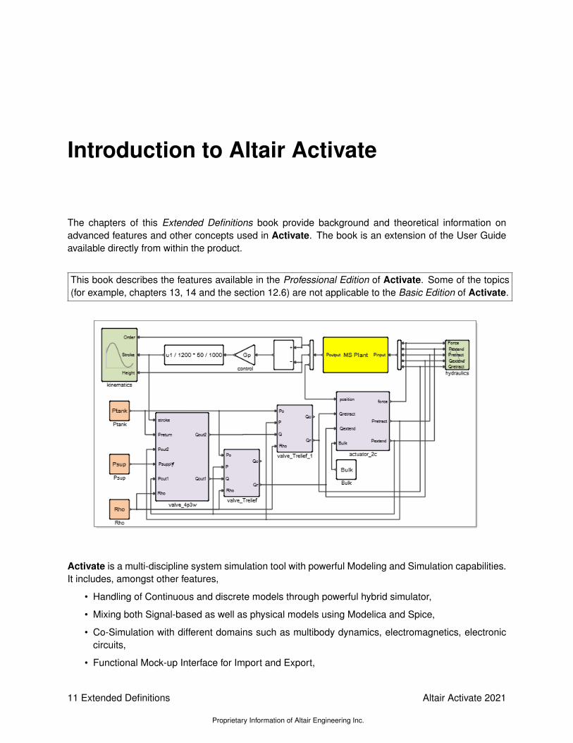
The chapters of this Extended Definitions book provide background and theoretical information onadvanced features and other concepts used in Activate. The book is an extension of the User Guideavailable directly from within the product.
This book describes the features available in the Professional Edition of Activate. Some of the topics(for example, chapters 13, 14 and the section 12.6) are not applicable to the Basic Edition of Activate.
Activate is a multi-discipline system simulation tool with powerful Modeling and Simulation capabilities.It includes, amongst other features,
• Handling of Continuous and discrete models through powerful hybrid simulator,
• Mixing both Signal-based as well as physical models using Modelica and Spice,
• Co-Simulation with different domains such as multibody dynamics, electromagnetics, electroniccircuits,
• Functional Mock-up Interface for Import and Export,
11 Extended Definitions
Proprietary Information of Altair Engineering Inc.
Altair Activate 2021

• Library Management,
• Code generation capabilities,
• Strong scripting language integration
Note - All models used in this book can be found in the installation directory under:/tutorial_models/Extended_Book_Models/.
Altair Activate 2021
Proprietary Information of Altair Engineering Inc.
Extended Definitions 12

Chapter 1
Activation signals in Altair Activate
1.1 Introduction
Activation signals in Activate control the execution of block functions. These signals can be explicitlymanipulated providing powerful modeling capabilities not available in other simulation environments.Here we provide an introduction to the role that Activation signals play in the Activate environment andpresent, through simple examples, their usage in modeling certain types of systems.
Associated with red links connected to ports usually placed on top and at the bottom of blocks, Activationsignals are present in most Activate diagrams. The most common usage is the activation of blocks ata fixed frequency with a signal generated by a SampleClock block. This block generates a series ofisolated activations, called events, regularly spaced in time.
Figure 1.1: Event Delay model (Eventdelay.scm)
Events can be explicitly operated on in Activate: they can be conditionally subsampled, and the unionand intersection of events can be constructed. Blocks can generate delayed events, allowing for exam-ple the implementation of operations such as event delaying. In the EventDelay model shown above,
13 Extended Definitions
Proprietary Information of Altair Engineering Inc.
Altair Activate 2021
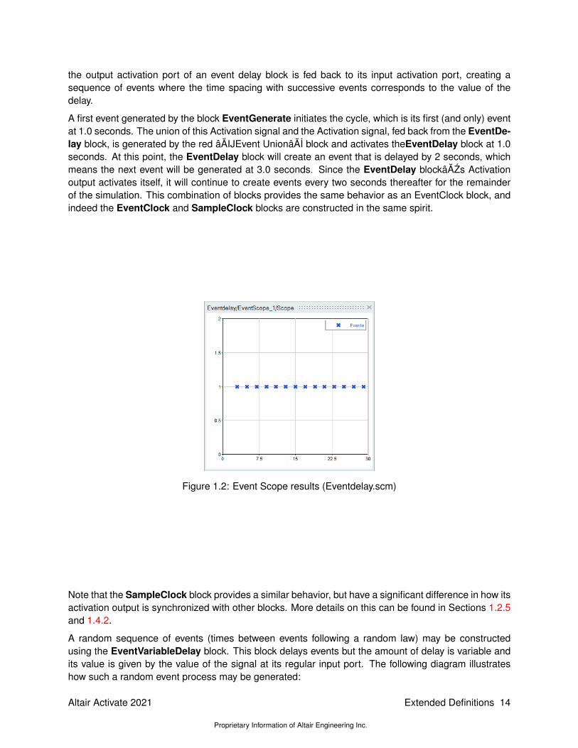
the output activation port of an event delay block is fed back to its input activation port, creating asequence of events where the time spacing with successive events corresponds to the value of thedelay.
A first event generated by the block EventGenerate initiates the cycle, which is its first (and only) eventat 1.0 seconds. The union of this Activation signal and the Activation signal, fed back from the EventDe-lay block, is generated by the red âAIJEvent UnionâAI block and activates theEventDelay block at 1.0seconds. At this point, the EventDelay block will create an event that is delayed by 2 seconds, whichmeans the next event will be generated at 3.0 seconds. Since the EventDelay blockâAZs Activationoutput activates itself, it will continue to create events every two seconds thereafter for the remainderof the simulation. This combination of blocks provides the same behavior as an EventClock block, andindeed the EventClock and SampleClock blocks are constructed in the same spirit.
Figure 1.2: Event Scope results (Eventdelay.scm)
Note that the SampleClock block provides a similar behavior, but have a significant difference in how itsactivation output is synchronized with other blocks. More details on this can be found in Sections 1.2.5and 1.4.2.
A random sequence of events (times between events following a random law) may be constructedusing the EventVariableDelay block. This block delays events but the amount of delay is variable andits value is given by the value of the signal at its regular input port. The following diagram illustrateshow such a random event process may be generated:
Altair Activate 2021
Proprietary Information of Altair Engineering Inc.
Extended Definitions 14

Figure 1.3: Random Event Delay model (RandEventdelay.scm)
Figure 1.4: Event Scope results (Eventdelay.scm)
If the random law representing the inter-event times follows the exponential law then the random eventprocess is a Poisson process. The Poisson process is often used in the modeling of queuing systems,for example to study the waiting time and queue size at Supermarket checkout lines.
1.1.1 Simple queue
A very simple model for a supermarket with a single checkout counter can be constructed as shown infigure 1.5
15 Extended Definitions
Proprietary Information of Altair Engineering Inc.
Altair Activate 2021

Figure 1.5: Simple Queuing model (Queue.scm)
The arrivals here are modeled as shown previously but using an exponential law (see figure 1.6).
Figure 1.6: Arrival super block in Simple Queuing model
The initial event starts the generation of arrival events.
But departures are slightly more complicated to model, even if exponential service time is considered.The reason is that unlike arrivals, departures may be halted, in particular when the queue is empty.Thus the state of the queue is required for modeling the departure process. As long as the queue isnot empty, the departure process operates similarly to the arrival process: the feedback loop generatessuccessive events. But when the queue is emptied, the feedback loop should be broken; no eventshould be generated in such a situation. When the queue is empty, a departure occurs only following anarrival. So the generation of the departure process depends also on the arrivals, in particular when the
Altair Activate 2021
Proprietary Information of Altair Engineering Inc.
Extended Definitions 16

queue contains a single element (it has been empty and an arrival has just occurred). The departurediagram contains, in addition to the Activation input used to initialize the process (as in the case ofarrivals) a second input receiving the arrival process. This Activation signal is filtered by an IfThenElseblock. The Activation signal from the “Else” branch, corresponding to the case where the state of queueis 1, is used for generating departure events. Another IfThenElse block is used to filter out events if thequeue is empty (figure 1.7).
Figure 1.7: Departure super block in Simple Queuing model
At each event activation, the state of the buffer is updated displayed by the Scope block. It is obtainedas the sum of the output of the SelectInput block and the previous state of the buffer (stored in theDiscreteDelay block. The SelectInput block copies one of its inputs to its output depending on theway by which it is activated. In particular if it is activated by an arrival event, the value of +1 is copiedto the output. If it is activated by a departure event, the value of −1 is copied. The initial event copiesthe value 0 (an unconnected input is assumed to have value 0 in Activate).
The simulation result shown in figure 1.8 gives the evolution of the state of the queue for the case ofexponential service time.
It is of course simple to replace the exponential random delay with a constant delay or a more complexexpression such as the sum of a constant with a random value. Indeed a realistic service time at acounter includes a time for payment which a priori does not depend on the number of purchased itemsand thus may be considered constant.
A useful block for modeling event sequences is the EventDelayedChannel. The EventDelay andEventVariableDelay blocks cannot be used to delay a train of events unless the delay is smaller thanthe time between two incoming events. The reason is that if an event is received by any of these blockbefore the event programmed on its output is fired, the output event is reprogrammed and the previousevent is lost. This has not been a limitation in the models considered previously but in some applications
17 Extended Definitions
Proprietary Information of Altair Engineering Inc.
Altair Activate 2021

Figure 1.8: Queue state evolution vs. time
the EventDelayedChannel block must be used to delay Activation signals.
1.1.2 Traffic simulation
Consider modeling the traffic, as for example in figure 1.9. Each traffic light on a road may be modeledas a queuing system with each event corresponding to a vehicle.
Figure 1.9: Circulation simulation model (Circul.scm)
Traffic light Super Blocks model the arrival and departure of cars (events). The regular output indicatesthe number of cars waiting behind the light. The road from one light to the next can be modeled usingan EventDelayedChannel block where a travel time may be associated with each vehicle on the road.
Altair Activate 2021
Proprietary Information of Altair Engineering Inc.
Extended Definitions 18

Unlike EventDelay blocks, EventDelayedChannel block contains an internal buffer that can be usedto store the state of individual vehicles on the road between the two traffic lights. Note that cars onthe road can travel at different speeds and pass each other. The road Super Block models the roadassuming that the travel time of each car is an independent random number (see figure 1.10).
Figure 1.10: road super block in Circulation model
The numbers of vehicles, as a function of time, waiting behind the two lights are displayed by the scopeand are illustrated below in figure 1.11
Figure 1.11: Number of vehicles behind the traffic lights
This paradigm may be used to model more complex queuing systems such as multiple dependentqueues, finite capacity queue buffers, and complex timing models. Such models may be used to studystochastic properties of complex queuing systems and optimize control strategies via for example MonteCarlo methods.
Events may also be used in models of systems usually seen as finite state machines. Consider forexample a simple thermostat-based cooling system that functions as follows: when the temperaturegoes above certain threshold value, it waits for a fixed amount of time and then turns on the coolingsystem unless in the meantime the temperature has dropped below the threshold value. For that,the block EventVariableDelay, and in particular its reprogramming capability may be used (see figure1.12).
In this "Plant" diagram, when the output of the Sum block becomes positive, i.e., the temperaturegoes beyond the threshold temperature, one of the EdgeTrigger block generates an event which isprogrammed for deltaT unit of time later, at the output of the EventVariableDelay block. If the output
19 Extended Definitions
Proprietary Information of Altair Engineering Inc.
Altair Activate 2021

Figure 1.12: Plant super block in Cooling model (Cooling.scm)
of the Sum block becomes negative before this event is fired, or a “restart” event is received, theoutput event of the EventVariableDelay block is reprogrammed, in this case de-programmed sinceprogramming with a negative delay corresponds to not programming any event.
The Super Block “Cooling System” at the bottom of the diagram generates the on/off command that isactually sent to the device. The strategy is as follows: when the “on” or “restart” event is received, thecooling system is turned on for a fix period CPer of time. At the end of this period, if the temperatureis still above the threshold temperature then the cooling system is turned off, otherwise it stays on foranother CPer unit of time.
Note that the CPer period where the output is on may be repeated multiple times before the tempera-tures goes below the threshold value.
There are of course specialized tools for modeling these types of systems, what makes event model-ing in Activate particularly powerful is its ability to combine events, and continuous and discrete-timedynamical systems. Events may be used to create discontinuities in the dynamics of the system, andevents may be generated by the dynamics. For example the thermostat model discussed previouslyis usually combined with a continuous-time model describing the action of the cooling system and theevolution of the temperature. A simple example is shown in figure 1.14.
The output of the integrator represents the room temperature. The simulation result is displayed infigure 1.15.
Altair Activate 2021
Proprietary Information of Altair Engineering Inc.
Extended Definitions 20

Figure 1.13: Cooling System super block (inside Plant) in Cooling model
1.1.3 Re-initialization of continuous-time state
The following example shows how an event can be used to re-initialize a continuous-time state. Thisexample corresponds to a model of a hormone-releasing hormone pulse generator proposed in [1]. AActivate model has been presented in [2].
The following diagram (figure 1.16) models a Super Block, named Pulse Generator, which providesboth the event and the value of the jump corresponding to the event.
The outputs of this block are used to create a jump in the state of the system.
The complete model including the Pulse Generator Super Block is shown in figure 1.17.
The nonlinear dynamics of the system modeled by MathExpression blocks are as follows
v = s(−v(v − c)(v − 1)− k1g + k2a),
g = b(v)(k3a+ k4v − k5g),
z = p(v)− k6z,
where
b(v) = b1 −b2
1 + exp(−b3(v − b4))and
p(v) =p1
1 + exp(−p2(h(v)− p3))with h(v) = v if v > 0 and h(v) = 0 otherwise. The s, a, ki, pi and, bi are model parameters.
The JumpStateSpace block is used to store the system state and model its re-initialization. In theabsence of activation on its input activation port, this block realizes a standard continuous-time linearsystem (in this case a simple integrator) with system input corresponding to the first input of the block.When activated through its activation port, the the state jumps to the value specified on the secondinput. In this case the state is x = (v, g, z). The simulation results are given in figure 1.18.
21 Extended Definitions
Proprietary Information of Altair Engineering Inc.
Altair Activate 2021

Figure 1.14: Cooling System model (Cooling.scm)
1.1.4 Communication delay
The ability to explicitly operate on Activation signals may also be used for studying the effects of com-munication delays in for example control systems. Consider a classical inverted pendulum controllerwith state feedback control (figure 1.19). The feedback is sampled and held over periods of 0.15 unit oftime.
Altair Activate 2021
Proprietary Information of Altair Engineering Inc.
Extended Definitions 22

Figure 1.15: Room Temperature vs. Time
Figure 1.19: Inverse pendulum with delay model (PendInvcdelay.scm)
If the initial state is not far from the equilibrium state, then this controller is capable of stabilizing thesystem:
23 Extended Definitions
Proprietary Information of Altair Engineering Inc.
Altair Activate 2021

Figure 1.16: Pulse Generator superblock in lut.scm model
Figure 1.20: Results of Inverse pendulum with delay model (PendInvcdelay.scm)
To study the effects of communication delay in the application of the control signal, the model can bemodified by applying a constant delay to the control signal. Since the control signal is a discrete signal,this can be done with a simple EventDelay block or a EventVariableDelay block with a constant input,as long as the amount of delay is less than the sampling period. Recall from Section 1.1.1, that if anevent is received by this block before the event programmed on its output is fired, the output event isreprogrammed and the previous event is lost.
Altair Activate 2021
Proprietary Information of Altair Engineering Inc.
Extended Definitions 24

Figure 1.17: Hormone releasing model (lut.scm)
Figure 1.21: Inverse pendulum with delay model, variant 1 (PendInvcdelay01.scm)
With a delay of 0.01, the system remains stable but the convergence to the steady-state position takesmore time:
25 Extended Definitions
Proprietary Information of Altair Engineering Inc.
Altair Activate 2021

Figure 1.18: Results for the Hormone releasing model
Figure 1.22: Results of Inverse pendulum with delay model, variant 1 (PendInvcdelay01.scm)
Increasing the delay to 0.02 completely destabilizes the system:
Altair Activate 2021
Proprietary Information of Altair Engineering Inc.
Extended Definitions 26

Figure 1.23: Results of Inverse pendulum with delay model, variant 2 (PendInvcdelay02.scm)
The model can be modified to study the effect of jitter (random delay) as shown in figure 1.24:
Figure 1.24: Inverse pendulum with random delay model (PendInvrdelay.scm)
This is done by feeding the EventVariableDelay block with a random signal instead of a constant.
If the amount of delay is larger than the sampling period, the EventDelayedChannel block must beused to model the behavior of the system.
27 Extended Definitions
Proprietary Information of Altair Engineering Inc.
Altair Activate 2021

1.2 Types of activation signals
Activation signals are used to specify activation times of the blocks they are connected to. Activatesupports different types of activation signals.
1.2.1 Programmed events
Activation signals seen so far were mostly isolated timed events generated by blocks activated by otherisolated timed events. These events were programmed in particular for given times in the future usingthe event delay blocks EventDelay and EventVariableDelay. When activated, Activate blocks canprogram output events on their activation output ports. The block in particular specifies the event firingdelay, i.e., how much time after the block execution the event should fire, for each of its output activationports.
The block may also program initial output events. The block EventGenerate for example programs onlyinitial events. It does nothing during simulation.
The time of a programmed event may be modified and the event may even be deprogrammed by theblock before the firing time. This is done simply by programming a new output event by indicatingthe new firing delay. This operation overwrites the previously programmed event because only oneevent can be programmed at any time for any output activation port. Giving a negative delay valuedeprograms the event. When an event is re- or de-programmed, a warning is issued by the simulator.
1.2.2 Zero-crossing events
Activation signals may also be produced by blocks activated in continuous-time. The EdgeTrigger blockseen previously is an example where an activation signal is produced based on a zero-crossing test.Such events are generated when a signal crosses a given surface, in general the surface correspondingto the value 0. A number of blocks in Activate palettes implement zero-crossing functionalities. Figure1.25 represents the simple model of a thermostat and its results (figure 1.26).
Zero-crossing blocks are used to turn on the heater or the cooler when the temperature falls below -10or rises above 10. The +to− and −to+ blocks generate events when the input of the block crosseszero respectively with a negative and a positive slope. The events activate the SelectInput block,which depending on the activation port through which it has been activated copies its first or secondinput (value -6 or +6) to its output. This output is the heat flow that is added to a random signal and fedto an integrator, the output of which represents the temperature. The simulation results show how thethermostat functionality is implemented by the zero-crossing blocks.
1.2.3 Continuous-time activation signal
The activation signals so far encountered are series of events, which are isolated activation signals intime. But activation signals are more general and include time intervals. The simplest activation signalof this type is the always active activation signal. The SampleClock block with period zero generatesthe always active activation signal; blocks that should be always active may be activated using thissignal.
Altair Activate 2021
Proprietary Information of Altair Engineering Inc.
Extended Definitions 28
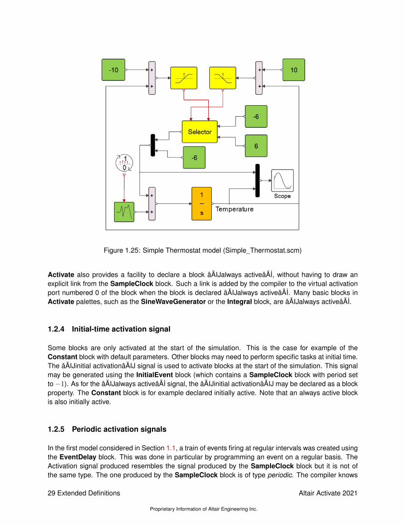
Figure 1.25: Simple Thermostat model (Simple_Thermostat.scm)
Activate also provides a facility to declare a block âAIJalways activeâAI, without having to draw anexplicit link from the SampleClock block. Such a link is added by the compiler to the virtual activationport numbered 0 of the block when the block is declared âAIJalways activeâAI. Many basic blocks inActivate palettes, such as the SineWaveGenerator or the Integral block, are âAIJalways activeâAI.
1.2.4 Initial-time activation signal
Some blocks are only activated at the start of the simulation. This is the case for example of theConstant block with default parameters. Other blocks may need to perform specific tasks at initial time.The âAIJinitial activationâAIJ signal is used to activate blocks at the start of the simulation. This signalmay be generated using the InitialEvent block (which contains a SampleClock block with period setto −1). As for the âAIJalways activeâAI signal, the âAIJinitial activationâAIJ may be declared as a blockproperty. The Constant block is for example declared initially active. Note that an always active blockis also initially active.
1.2.5 Periodic activation signals
In the first model considered in Section 1.1, a train of events firing at regular intervals was created usingthe EventDelay block. This was done in particular by programming an event on a regular basis. TheActivation signal produced resembles the signal produced by the SampleClock block but it is not ofthe same type. The one produced by the SampleClock block is of type periodic. The compiler knows
29 Extended Definitions
Proprietary Information of Altair Engineering Inc.
Altair Activate 2021

Figure 1.26: Results from Simple Thermostat model (Simple_Thermostat.scm)
that this signal is periodic contrary to the signal produced by the EventDelay block, which happens tocontain events firing periodically thanks to the way the model is constructed.
An Activation signal is said to be periodic only if it is of type periodic.
Strictly speaking a SampleClock block is not a regular Activate block. Not only does it produce Acti-vation signals that are periodic but also synchronous (see Section 1.4).
The Activate compiler has a special treatment for periodic activation signals. Some Activate blocksoperate only on periodic activation signals. When a block is activated by a periodic signal, it has accessto the period and offset information at compile time. Thanks to this information, the block can adaptits behavior by computing specific block simulation parameters.The SampledData block for examplecomputes the discrete-time linear system matrices corresponding to the discretization of a continuous-time linear system for the operating frequency. This frequency, which is the inverse of the sampling(activation) period, is available at compile time. This block cannot function if it is activated by a non-periodic activation signal.
The only blocks producing periodic activation signals are the SampleClock and the ReSampleClockblocks.
1.3 Activation inheritance
Specifying explicitly the activation signals of the blocks in the model is useful for specifying the modelbehavior unambiguously. But doing it systematically could make the model labyrinthian. In some casesthe explicit graphical presence of activation links is not necessary for the comprehension of the modelbehavior. The ability to declare blocks initially active or always active is one mechanism to simplify themodel by removing some activation links. The other mechanism is inheritance.
The inheritance mechanism is an editor facility that can be used to reduce significantly the number ofactivation links in models. Most basic blocks in Activate may be both explicitly activated or activated byinheritance. Whether the block works by inheritance or external activation is specified via the âAIJEx-ternal activationâAI checkbox in the block parameter GUI. When the box is checked, the input activationport is added; unchecked, the block inherits its activation. For example, see the Scope block.
Altair Activate 2021
Proprietary Information of Altair Engineering Inc.
Extended Definitions 30

A block inherits its activation if it has no activation input ports and it is not declared always active. Ablock that inherits, either receives the union of the activations of all the blocks that provide its inputs onits only (invisible) input activation port, or receives the activations associated with each of its input on aseparate (invisible) input activation port. The former is the default behavior. Indeed most blocks don’tbehave differently depending on the port through which they have been activated.
Consider the following model described in figure 1.27.
Figure 1.27: Model illustrating inheritance
The yellow colored blocks inherit their activations. The yellow Power block has one input so its inher-itance yields the exact behavior as that of the orange colored Power block. The yellow Sum blockhas two inputs and has default inheritance property so it is activated by the union of the activationsgenerated by the two SampleClock blocks, as in the case of the orange colored Sum block. This is theproper inheritance property for the Sum block since no matter which input of the block is modified, thesame summation operation must be performed.
The SelectInput block on the other hand has naturally multiple activation input ports. The block copiesone of its inputs to its output depending on the port by which it has been activated. So the inheritanceproperty of the SelectInput block is necessarily different from that of the Sum block. Its behavior is thatof the orange colored SelectInput block.
1.4 Synchronous vs. asynchronous activations
Activation signals are characterized by time periods and instances. An event for example defines an iso-lated point in time specifying the time instant when the block(s) receiving the event should be activated.The time of the event however does not completely characterize the event, and in particular its relation-ship with other events. In particular, two events may have identical times but not be synchronous. Thedistinction between synchronicity and simultaneity is a subtle but important point to understand since itplays a fundamental role in the semantic specification of the graphical language.
31 Extended Definitions
Proprietary Information of Altair Engineering Inc.
Altair Activate 2021

When two blocks are activated by the same event the compiler must compute the order in which theymust be activated depending on the way they are connected to each other. In particular if one of theblocks requires the value on one of its inputs for computing its output and this input is connected to theoutput of other block, then the latter block should be executed first. In general, for any activation signalthe compiler computes a table to specify the list of the blocks to be executed and the order in whichthey have to be executed. The list includes the blocks receiving the activation signal directly or indirectlythrough inheritance or the ExtractActivation block.
Each “distinct” activation source then has its own list of blocks and is treated independently of otheractivation sources. Even if two events produced by two “distinct” activation sources happen to haveidentical times, they are treated independent event. At run time, the two events are treated sequen-tially. Two “distinct” activation sources produce asynchronous activation signals. The notion of “distinct”activation sources however needs clarification. In general any output activation port on a Activate isconsidered a distinct activation source. There are however exceptions:
1.4.1 Conditional blocks
Two Activate blocks play a very special role in the construction of models. Strictly speaking conditionalblocks are not Activate blocks but are graphically represented as such to facilitate their usage. Tomake an analogy with classical programming languages such as C where blocks represent functioncalls, conditional blocks represent the conditional constructs: if and switch case statements. TheIfThenElse block has one activation input port and two activation output ports. Depending on thevalue of the signal on its regular input port, the “block” redirects its input activations to one of its outputactivation ports. In this case, the output activation signal is synchronous with the input activation signal.So the compiler cannot treat the output activation ports of the IfThenElse block as “distinct” activationsources.
The SwitchCase block is the other conditional block in Activate. This block may have more than twooutput activation ports and the input activation signal is redirected to one of them depending on thevalue of the regular input of the block at the time of execution.
1.4.2 Sample and Resample Clock blocks
The SampleClock and ReSampleClock blocks are not regular blocks either. These “blocks” producea train of events with specified phase and period, just as the EventClock block does. The EventClockis essentially a Super Block containing an EventDelay with feedback. But unlike the EventClock,the activation signals produced by multiple SampleClock and ReSampleClock blocks may be syn-chronous. The compiler replaces the synchronous SampleClock and ReSampleClock blocks with aunique EventClock and subsampling mechanisms using conditional blocks to produce synchronousactivation signals corresponding to the outputs of all the SampleClock and ReSampleClock blocks.
SampleClock and ReSampleClock blocks are considered synchronous throughout the model unlessthe model contains SyncTag blocks. If a diagram contains a SyncTag block, then the SampleClockand ReSampleClock blocks inside the diagram are not considered synchronous with SampleClockand ReSampleClock blocks outside the diagram (but they remain synchronous among themselves inthe absence of other SyncTag blocks).
Note that conditional and Sample blocks may be hidden inside Super Blocks. In particular the Fre-quencyDivider and EdgeTrigger blocks in Activate palettes generate synchronous activation signals
Altair Activate 2021
Proprietary Information of Altair Engineering Inc.
Extended Definitions 32

because they include conditional blocks.
33 Extended Definitions
Proprietary Information of Altair Engineering Inc.
Altair Activate 2021

Altair Activate 2021
Proprietary Information of Altair Engineering Inc.
Extended Definitions 34

Bibliography
[1] D. Brown et al., Modelling the Luteinizing Hormone-Releasing Hormone Pulse Generator. Neuro-science, Vol 63, no 3, 1994.
[2] S.L. Campbell, J.Ph. Chancelier and R. Nikoukhah, Modeling and Simulation in Scilab/Scicos withScicosLab 4.4. Springer, 2010.
35 Extended Definitions
Proprietary Information of Altair Engineering Inc.
Altair Activate 2021

Altair Activate 2021
Proprietary Information of Altair Engineering Inc.
Extended Definitions 36
Chapter 2
Altair Activate Matrix Expression Block
2.1 Introduction
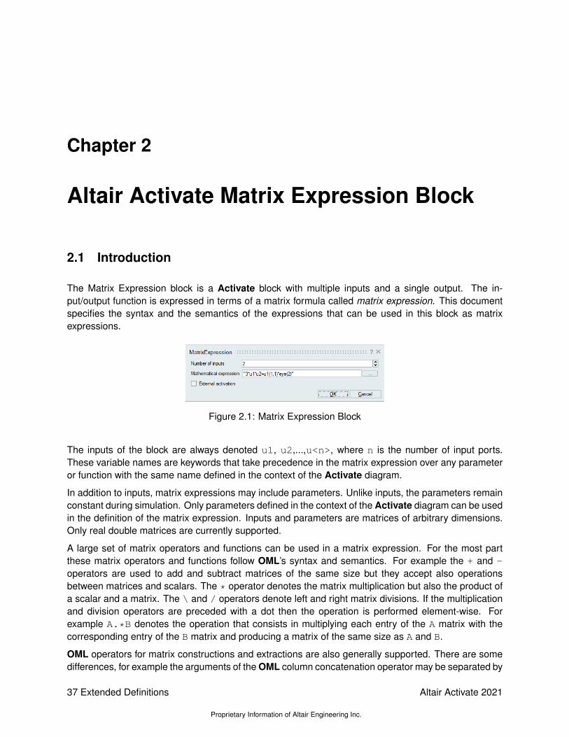
The Matrix Expression block is a Activate block with multiple inputs and a single output. The in-put/output function is expressed in terms of a matrix formula called matrix expression. This documentspecifies the syntax and the semantics of the expressions that can be used in this block as matrixexpressions.
Figure 2.1: Matrix Expression Block
The inputs of the block are always denoted u1, u2,...,u<n>, where n is the number of input ports.These variable names are keywords that take precedence in the matrix expression over any parameteror function with the same name defined in the context of the Activate diagram.
In addition to inputs, matrix expressions may include parameters. Unlike inputs, the parameters remainconstant during simulation. Only parameters defined in the context of the Activate diagram can be usedin the definition of the matrix expression. Inputs and parameters are matrices of arbitrary dimensions.Only real double matrices are currently supported.
A large set of matrix operators and functions can be used in a matrix expression. For the most partthese matrix operators and functions follow OML’s syntax and semantics. For example the + and -operators are used to add and subtract matrices of the same size but they accept also operationsbetween matrices and scalars. The * operator denotes the matrix multiplication but also the product ofa scalar and a matrix. The \ and / operators denote left and right matrix divisions. If the multiplicationand division operators are preceded with a dot then the operation is performed element-wise. Forexample A.*B denotes the operation that consists in multiplying each entry of the A matrix with thecorresponding entry of the B matrix and producing a matrix of the same size as A and B.
OML operators for matrix constructions and extractions are also generally supported. There are somedifferences, for example the arguments of the OML column concatenation operator may be separated by
37 Extended Definitions
Proprietary Information of Altair Engineering Inc.
Altair Activate 2021

commas or spaces whereas only comma-separated arguments are supported in the matrix expressionblock (for example in the matrix expression block, the valid OML concatenation operation [A B] mustbe expressed as [A,B], which is also a valid OML expression). In some cases the matrix expressionblock is less restrictive than OML.
Most mathematical functions such as sin, cos, exp, accept matrix arguments in which case thefunction is applied to each entry of the matrix.
The list of these operators and supported functions are given in Sections 2.6 and 2.7.1. In additionto supported functions, any OML function available in the context of the diagram (both basic OMLfunctions and user defined functions) can be used as long as their arguments do not depend on thevalues of the block inputs. These functions are evaluated once at compilation time. String argumentsof such functions must be expressed with double quotes and not single quotes as in OML.
2.2 Examples
Matrix Expressions are similar to OML expressions with some restrictions and some extensions.
2.2.1 Basic operators and functions
Matrix addition and multiplication The expression
u1’*u2
is the matrix product of u1 transpose and u2. This is a valid expression if u1 and u2 have the samenumber of rows, or if one is one-by-one, i.e., is a scalar.
The expression
A*u1+u2
when the parameter A is defined in the context of the Activate diagram containing the block is valid ifthe dimensions of matrices A, u1 and u2 are compatible. Note that the product A*u1 is consideredvalid if the number of columns of A equals the number of rows of u1, or if A or u1 is scalar. Similarly,the sum A*u1+u2 is valid if either both terms of the sum have identical dimensions, or one is scalar.
Element-wise operators and functions If matrix inputs u1 and u2 have equal size, the expression
(u1.*u2)./(u1.^2+u2.^2)
returns a matrix of the same size. The (i, j) entry of the result is equal to the product of the (i, j) entriesof u1 and u2 divided by the sum of their squares.
The expression
u1>3
generates a matrix having the size of u1 and including ones and zeros depending on whether thecorresponding entry in u1 is larger than 3 or not.
The expression
sin(u1)
Altair Activate 2021
Proprietary Information of Altair Engineering Inc.
Extended Definitions 38

returns a matrix having the size of u1 with entries equal to the sine of the corresponding entry in u1.
If expression Conditional statements in OML are not expressions and are not supported. Howevermatrix expression supports expressional if statements, and in particular their extension to the matrixcase, where the conditions are applied elementwise. The keywords .if, .then and .else are usedin the expressional if statements. The condition and the values returned in the .then and .elsebranches are normally matrices of identical dimensions however a scalar can also be used in whichcase it is (conceptually) expanded to a matrix.
For example the expression:
.if u1<0 .then u1 .else 0 .end
returns a matrix equal to u1 in which the negative entries are set to zero.
Switch expression Similarly the ’switch’ clause is expressional and is extended to the matrix case.For example the expression:
.switch u1.case a, u1.case b, -u1.otherwise 0
.end
implements an element-wise switch expression.
2.2.2 Matrix construction, extraction and assignment
Matrix construction Commas (for column concatenation) and semi-colons (for row concatenation)are used to construct matrices from other matrices (or scalars which are just one-by-one matrices).This is similar to constructing matrices in OML. For example:
[u1,1;u2]
is valid provided u1 has one row and that the number of columns of u2 exceeds that of u1 by one.
Extracting a sub-matrix A submatrix of a matrix can be specified by indicating the row and columnindices to be extracted. For example
u1([1,3],2)
returns the two-by-one matrix [u1(1,2);u1(3,2)].
The extraction operator can also be used for repeating rows and columns or changing their positions.For example if u1 is a two-by-two matrix
u1([1,1,1,2,2,2],[1,2])
returns a six-by-two matrix where each column is repeated three times and the rows are switched.
Single index extraction is also possible:
u1(2:n)
39 Extended Definitions
Proprietary Information of Altair Engineering Inc.
Altair Activate 2021
The matrix u1 is seen as a vector containing the entries of the matrix aligned column-wise so the resultis a column vector, unless u1 is a row vector in which case the output is a row vector.
Special operators The use of the keyword end and the symbol ’:’ simplify matrix expressions byallowing to refer to the last element or all the elements of a row or a column of a matrix without havingto explicitly compute its size. For example
[u1(1,end);u2(end-1,:)]
returns the concatenation of the first row of u1 with the one-before-the-last row of u2.
The ’end’ indicates the last row or column element depending on whether it is used in the first or secondargument of the extraction operation, and ’:’ denotes all the elements of the row or column. In the caseof single index extraction, ’end’ indicates the last element (last row element of the last column) and ’:’all the elements of the matrix.
The symbol ’$’ may also be used in place of ’end’.
Matrix assignment and row column deletion The ’=’ sign is not used in the matrix expression sinceunlike in a OML script, an expression does not define intermediary variables. The matrix assignmentoperator ’:=’ however allows modifying entries of an existing matrix similar to the OML instructionA(exp1,exp2)=exp3. For example the following expression
u1(:,1):=3
returns a matrix identical to u1 with all the elements of its first column set to 3. The right hand side ofthe ’:=’ operator should have the same size as the submatrix designated by the left hand side, or be ascalar.
Row and columns can be deleted by assigning an empty matrix to them. For example
u1(:,[1,3]):=[]
removes the first and third columns. Note that
u1(:,u2):=[]
is compiled but results in run-time error if any entry of u2 becomes less than or equal to zero, orbecomes bigger than the number of columns of u1. A run-time error is also generated if two entries ofu2 (casted into integers) become identical. The reason is that the size of the result would then changeduring simulation. This violates the fixed-sized matrix principle discussed later.
2.2.3 Use of OML functions
Functions other than those listed in Section 2.6 may be used if they are OML functions available in thecontext of the Activate diagram containing the Matrix Expression block. These OML functions can beused only if their arguments do not depend the block inputs; for example the expression
[u1;HammWin(L)]
is valid (the argument of the Hamming Window function, L must be defined, for example in the contextof the diagram). In this case, this parameter is available at compile time and its value does not changeduring the simulation, contrary to u1. Note however that even though u1 may vary in time, its size
Altair Activate 2021
Proprietary Information of Altair Engineering Inc.
Extended Definitions 40

cannot. So
[u1;HammWin(size(u1,2))]
is also valid.
Only memoryless OML functions should be used because these functions are evaluated by OML onlyonce. So for example the expression
UnifRnd()
does not produce a random signal during simulation but rather a random output that remains constantduring the simulation, contrary to what the user may expect.
2.3 Parser
When the Activate diagram is compiled, the matrix expressions of the Matrix Expression blocks presentin the model are parsed and converted into pseudo-codes used for evaluation during simulation1. Theparser is similar to OML’s parser, in particular it uses the same rules of precedence, and allows for com-positions of functions and operators. This is an important feature for the definition of matrix expressionsfor which it is not possible to define intermediary variables. For example the OML code
a=C*u1*u2=a(1,2)
can be expressed (as in OML) as a single expression as follows
(C*u1*u2)(1,2)
There is no limit as to the level of composition allowed, for example expressions such as
[inv([u1,u2])(1,:)*u2,u2(1)]’(2)
are valid.
Matrix expressions can be expressed over multiple lines. But line breaks and spaces are not separators:in particular spaces cannot be used as matrix column separators and line breaks cannot be used asrow separators. The valid OML expression
[u1 21 3]
is not valid as a matrix expression and must be expressed as follows
[u1, 2;1, 3]
1In the future, they will also be used for C code generation
41 Extended Definitions
Proprietary Information of Altair Engineering Inc.
Altair Activate 2021

2.4 Limitations
2.4.1 Fixed-sized matrix principle
Matrix sizes of all intermediary matrices obtained in the course of evaluating the matrix expression, andof course the final result, are determined at compile time so that no dynamic allocation is used duringsimulation. This places limitations on the types of expressions allowed. For example
[1:u1]
is not allowed since the size of the result depends on the value of u1 (the first input), which may changeduring simulation.
In some cases, even if the the size of the result does not depend on an input, the compiler cannotdetermine the size. For example the following expression is not accepted
[u1(end)+1:u1(end)+5]
and has to be re-written as follows
u1(end)+[1:5]
This means in particular that the expression
u2(u1(end)+[1:5])
is valid (but may produce a run-time out of index error during simulation depending on the value ofu1(end)).
2.4.2 All the branches of conditional expressions evaluated
The ’if’ and ’switch’ clauses are extended to the matrix case and applied element-wise, thus the outputmay depend on the expressions in multiple branches. That is why all the branch expressions are alwaysevaluated. For the same reason, logical or (|) and logical and (&) operators are not short circuited.
2.4.3 No support for logical type
The logical data type is not supported so the output of the relational and logical operations are con-sidered regular matrices (which happen to contain only zeros and ones). This means in particular thatmatrix extraction based on logical tests cannot be used. For example
u1(u1>3):=3
cannot be used to select the values of u1 that are larger than three and set them to 3. This can bedone using the element-wise if expression
.if u1>3 .then 3 .else u1 .end
Note that in this simple example the expression can also be implemented as follows
min(u1,3)
Altair Activate 2021
Proprietary Information of Altair Engineering Inc.
Extended Definitions 42

2.5 Data types
2.5.1 Supported data type
The basic numerical data type used in the evaluation of a matrix expression is the matrix of real num-bers coded as doubles (float64). The inputs, the output and all intermediary matrix evaluations duringsimulation use this data type. In particular, no distinction is made between a scalar and a one-by-onematrix.
Parameters defined in the diagram context can have any OML data types if in the matrix expressionthey are only used in the definition of the argument of a OML function that produces a matrix of realnumbers. Strings can also be used explicitly in defining the expression under the same condition. Forexample the expression
f(1,"row")*u1
is valid provided the OML function f is defined in the context and returns a real matrix with proper size.Note the usage of double-quotes for defining a string. OML uses single quotes to define strings.
The reason for which OML data types can be used under the above condition is that OML functions andin general expressions that do not depend on block inputs are evaluated at compile time by OML. Suchexpressions are then replaced with the resulting matrices of real numbers in the matrix expression.
2.5.2 Unsupported data types
As previously stated, only matrices of real numbers are supported by supported functions. In particularit should be noted that there is no support for the logical data type. The output of logical and relationaloperators are considered matrices of real numbers containing zeros and ones. In a logical operation,zero is considered false and any non-zero number is true.
Currently complex numbers are not supported.
2.5.3 Data coding
The matrix data is stored in column-major format in memory. All the operations and supported functionsuse the IEEE standard for 64-bit floating point arithmetic. The block however generates an error if theresult of the overall evaluation of the matrix expression, which is the output of the block, contains a NaN(Not a Number).
2.6 Supported operators
2.6.1 Arithmetic operators
The arithmetic operators available for matrix expressions are similar to those available in OML.
In the following tables, <exp> denotes any valid expression.
43 Extended Definitions
Proprietary Information of Altair Engineering Inc.
Altair Activate 2021
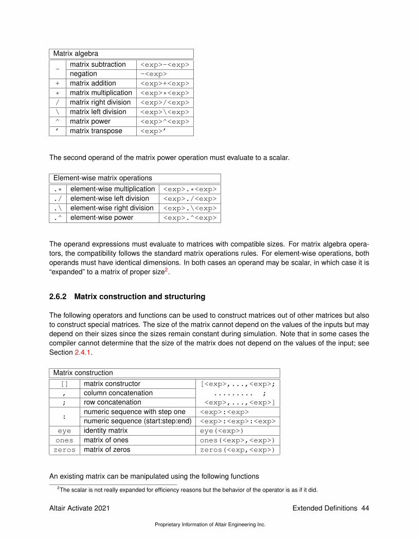
Matrix algebra
-matrix subtraction <exp>-<exp>negation -<exp>
+ matrix addition <exp>+<exp>
* matrix multiplication <exp>*<exp>/ matrix right division <exp>/<exp>\ matrix left division <exp>\<exp>^ matrix power <exp>^<exp>’ matrix transpose <exp>’
The second operand of the matrix power operation must evaluate to a scalar.
Element-wise matrix operations.* element-wise multiplication <exp>.*<exp>./ element-wise left division <exp>./<exp>.\ element-wise right division <exp>.\<exp>.^ element-wise power <exp>.^<exp>
The operand expressions must evaluate to matrices with compatible sizes. For matrix algebra opera-tors, the compatibility follows the standard matrix operations rules. For element-wise operations, bothoperands must have identical dimensions. In both cases an operand may be scalar, in which case it is“expanded” to a matrix of proper size2.
2.6.2 Matrix construction and structuring
The following operators and functions can be used to construct matrices out of other matrices but alsoto construct special matrices. The size of the matrix cannot depend on the values of the inputs but maydepend on their sizes since the sizes remain constant during simulation. Note that in some cases thecompiler cannot determine that the size of the matrix does not depend on the values of the input; seeSection 2.4.1.
Matrix construction[] matrix constructor [<exp>,...,<exp>;, column concatenation ......... ;; row concatenation <exp>,...,<exp>]
:numeric sequence with step one <exp>:<exp>numeric sequence (start:step:end) <exp>:<exp>:<exp>
eye identity matrix eye(<exp>)ones matrix of ones ones(<exp>,<exp>)zeros matrix of zeros zeros(<exp,<exp>)
An existing matrix can be manipulated using the following functions2The scalar is not really expanded for efficiency reasons but the behavior of the operator is as if it did.
Altair Activate 2021
Proprietary Information of Altair Engineering Inc.
Extended Definitions 44

Matrix extraction and assignment(,) sub-matrix extraction <exp>(<exp>,<exp>)() vector extraction <exp>(<exp>)
:all rows <exp>(:,<exp>)all columns <exp>(<exp>,:)all elements <exp>(:)
endlast row <exp>(end,<exp>)last column <exp>(<exp>,end)last element <exp>(end)
:=
entry assignment <exp>(<exp>):=<exp>column assignment <exp>(:,<exp>):=<exp>row assignment <exp>(<exp>,:):=<exp>row deletion <exp>(:,<exp>):=[]column deletion <exp>(<exp>,:):=[]
2.6.3 Relational and logical operators
The relational operators can be used to compare two matrices of the same size or a matrix and a scalar.In the latter case, the elements of the matrix are each compared with the scalar. In both cases, theresult is a matrix including ones and zeros.
Relational operators< element-wise less than <exp> < <exp>> element-wise greater than <exp> > <exp><= element-wise less than or equal <exp> <= <exp>>= element-wise greater than or equal <exp> >= <exp>== element-wise equal <exp> == <exp>~=
element-wise not equal<exp> ~= <exp>
<> <exp> <> <exp>
The logical operators produce ones and zeros but their arguments can be any number. The numberzero is considered false and any other number, true.
Logical operators| element-wise logical or <exp>|<exp>& element-wise logical and <exp>&<exp>~ element-wise logical not ~<exp>and logical and of all matrix elements and(<exp>)or logical or of all matrix elements or(<exp>)
45 Extended Definitions
Proprietary Information of Altair Engineering Inc.
Altair Activate 2021

2.6.4 Conditional operators
Conditional operators ’if’ and ’switch’ are extended to the matrix case. Note that expressions in allbranches of conditional operators are evaluated; see Section 2.4.2.
Element-wise if expression The element-wise if expression operates on matrices and behaves likea standard ’if’ expression for each entry of the matrix.
.if <cond_exp> .then <exp> .else <exp> .end
Normally all three expressions must have identical sizes. But one or two may be scalar. The result isa matrix with entries coming from the expressions in the ’then’ and ’else’ branches. In particular the(i, j) entry of the resulting matrix is equal to the (i, j) entry of the matrix obtained by evaluating theexpression in the ’then’ branch (or the value of the expression if it is a scalar) if the (i, j) entry of thematrix obtained by evaluating the condition expression <cond_exp> (or the value of the expression ifit is a scalar) is not zero. Otherwise it is equal to the (i, j) entry of the matrix obtained by evaluating theexpression in the ’else’ branch (or the value of the expression if it is a scalar).
Element-wise switch expression The element-wise switch expression is an extension of the element-wise if expression. The resulting matrix is composed of the entries of the matrices corresponding toexpressions returned in different cases.
.switch <cond_exp>.case <case_exp>, <exp>....case <case_exp>, <exp>.otherwise <exp>
.end
The (i, j) entry of the resulting matrix is equal to the (i, j) entry of the matrix obtained by evaluating theexpression in the branch where the (i, j) entry of the matrix obtained by evaluating the case expression<case_exp> is equal to the (i, j) entry of the matrix obtained by evaluating the condition expression<cond_exp>.
In case this (i, j) entry matches more than one cases, the first case is taken into account. If it matchesno case, the (i, j) entry of the resulting matrix is set to the (i, j) entry of the matrix obtained by evalu-ating the expression following .otherwise. The .otherwise "case" must always be present.
2.7 Supported functions
The syntax of a function call is
<fun>(<exp>,...,<expr>)
The list of arguments may be empty.
Altair Activate 2021
Proprietary Information of Altair Engineering Inc.
Extended Definitions 46

2.7.1 Supported functions
Supported functions listed in this section can be used in matrix expressions. Their arguments can beany valid expressions. If all the arguments of a function do not not depend on the values of the inputs,the function is evaluated only once at compile time.
Element-wise functions
The following functions apply to matrices by applying the corresponding scalar function to each elementof the matrix.
Trigonometric functionsacos inverse cosine acos(<exp>)acosh inverse hyperbolic cosine acosh(<exp>)asin inverse sine asin(<exp>)asinh inverse hyperbolic sine asinh(<exp>)atan inverse tangent abs(<exp>)atan2 four-quadrant inverse tangent atan2(<exp>,<exp>)atanh inverse hyperbolic tangent atanh(<exp>)cos cosine cos(<exp>)cosh hyperbolic cosine cosh(<exp>)hypot hypothenuse hypot(<exp>)sin sine sin(<exp>)sinh hyperbolic sine sinh(<exp>)tan tangent tan(<exp>)
Rounding functionsceil round up ceil(<exp>)floor round down floor(<exp>)int round toward zero int(<exp>)round round to nearest integer round(<exp>)
Other functionsabs absolute value abs(<exp>)exp exponential exp(<exp>)log natural logarithm log(<exp>)log10 base 10 logarithm log10(<exp>)max maximum max(<exp>,<exp>)min minimum min(<exp>,<exp>)sign sign (return -1,0 or 1) sign(<exp>)sqrt square-root sqrt(<exp>)
47 Extended Definitions
Proprietary Information of Altair Engineering Inc.
Altair Activate 2021

Matrix functions
The following matrix functions are available
Matrix functionsdet determinant of a square matrix det(<exp>)diag create diagonal matrix from vector or vice-versa diag(<exp>)expm matrix exponential of a square matrix expm(<exp>)inv matrix inversion of a square matrix inv(<exp>)logm matrix log of a square matrix logm(<exp>)
maxmaximum along rows unless argument is a row vectorin which case maximum of all entries
max(<exp>)
minminimum along rows unless argument is a row vectorin which case minimum of all entries
min(<exp>)
sizevector including both matrix dimensions size(<exp>)row dimension size(<exp>,1)column dimension size(<exp>,2)
sum
sum along rows unless argument is a row vectorin which case sum of all entries
sum(<exp>)
sum along rows sum(<exp>,1)sum along columns sum(<exp>,2)
svd singular values svd(<exp>)
2.7.2 Using OML functions
Any OML function available in the context of the Activate diagram containing the Matrix Expres-sion block can be used in the definition of its matrix expression provided the arguments of the func-tion do not depend on the values of the inputs. Note that size(<exp>), size(<exp>,1) andsize(<exp>,2) may be used in constructing the arguments of the OML function regardless ofwhether or not the argument of the size functions depend on the inputs. The reason is that the outputof size does not depend on the value of its argument.
Unlike for supported functions, a block parameter defined in a diagram context hides a OML function ifit has the same name.
Altair Activate 2021
Proprietary Information of Altair Engineering Inc.
Extended Definitions 48

Chapter 3
C and OML Custom Blocks in AltairActivate
Activate contains a large set of blocks organized in libraries and made available to the user through var-ious palettes. These blocks provide basic mathematical functions needed to construct complex modelsof dynamical systems and also provide access to some input/output functionalities for files, graphicalwidgets, etc. In some cases however, it may be required or more convenient to express dynamicalbehavior of a block programmatically in C or in (OML) language , for example to take advantage of ex-isting code or gaining access to OS functionalities in special ways. Constructing new Activate blocks ispossible in Activate and the procedure is presented in the Block Builder documentation. An alternativeto constructing a new block is using Custom blocks.
Custom blocks (C or OML) allow user to specify the dynamical behavior of the block in a block pa-rameter. The actual simulation source code of the block (C or OML) or a reference to correspondingshared library or OML file becomes a parameter value, which is stored in the model where the blockis used, and saved in the corresponding scm file. The model is thus self-contained -in other words,a library is not referenced by the block to define its behavior as is the case for most blocks. Indeed,CCustomBlock and OmlCustomBlock blocks are not new blocks.
So compared to creating and using new blocks, Custom blocks have the advantage of not requiring anylibrary management operations. But even though their look and feel may be customized to some extent(in particular by encapsulating them in a masked Super Block) Custom blocks are not always the bestsolution. With Custom blocks, there is no mechanism for automatically upgrading the code of Customblocks as there is for library blocks. Custom blocks are often used as a first step to develop and test Csimulation codes destined for new blocks.
Both CCustomBlock and OmlCustomBlock blocks also provide the option of not including the sourcecode of the simulation function. The simulation function of a CCustomBlock block may be provided bya shared library (dll file under Windows operating system). Instead of the C code, the block parametersinclude the path to the shared library and the name of the entry point. This option is particularlyinteresting for preserving intellectual property but note that the model is no longer self-contained. Theshared library file must be distributed along with the model.
Similarly for OmlCustomBlock blocks the OML code does not need provided. An OML file defining thefunction and its name may used as block parameters instead. If a file is not specified Activate assumesthat the function is already defined in the environment.
49 Extended Definitions
Proprietary Information of Altair Engineering Inc.
Altair Activate 2021

The MathExpression and MatrixExpression blocks should be considered before using Custom blockssince they provide even simpler ways to express the dynamical behavior of a block. They are howeverlimited to expressing stateless dynamics: block outputs depend on block inputs alone, and the expres-sions support a fixed set of functions that cannot be extended by the user.
3.1 Activate block simulation function
A Activate block is defined by its graphical properties (specified in XML), an OML code for its instan-tiation and parameterization, and its simulation routines which can be in C or OML. The Block Buildertool provides a user interface for interactively designing a new block, in particular its graphics, and theOML code for its instantiation and parameterization. For using the CCustomBlock and OML customblocks however users need not worry about these aspects; Custom blocks provide generic graphicsand parameters allowing users to focus on developing the simulation function.
Block simulation functions are called by the Activate simulator during simulation to perform differenttasks, such as updating the output or the state. Simulation functions have two arguments: block andflag. The task to be realized is specified by the argument flag. The argument block is a the block’sdata structure to be passed to the APIs to get and set block data. Block simulation code may be in C orOML.
3.2 Custom block parameter GUI
CCustomBlock and OmlCustomBlock blocks’ parameter GUIs provide an interactive user interfaceto define block properties. Users can define the number and types of inputs and outputs, the statesand simulation parameters (if any) and other properties. The interface also gives access to an editorfor writing the block’s simulation code.
Developing a simulation code requires a knowledge of the APIs needed to get and set block data,for example for reading block inputs and writing block outputs. But Custom blocks provide a utility togenerate a skeleton of the simulation code by taking into account the block properties specified by theuser. This significantly facilitates the development of the simulation code.
Block inputs, outputs and simulation parameters are named and the code skeleton generator takes intoaccount this information in order to provide a code where the user, in most cases, simply needs to addinstructions (in C or OML) involving the provided names as program variables. These variables arealready declared and initialized when needed.
The Custom block parameter GUI, illustrated in Fig. 3.1 (the C block; OML block is similar), could beconsidered as an interactive interface. It contains five tabs for customizing the properties of the block.
• Ports tab is used to specify the inputs and outputs of the block. For regular ports (not activationports), the port sizes, types, feedthrough properties and names can in particular be specified.
• States tab is used to initialize block states, both discrete and continuous-time. Discrete objectstates oz may be typed and named.
If the simulation function is declared to be implicit in the SimFunctions tab, the initial value of thecontinuous-time state derivative should also be specified.
Altair Activate 2021
Proprietary Information of Altair Engineering Inc.
Extended Definitions 50

Figure 3.1: Block parameter GUI of CCustomBlock block.
• Parameters tab is used to set the value of rpar and ipar parameters; a list of opar parametersmay also be defined, typed and named.
These parameters are simulation parameters that are available to the simulation function. Theobject parameters (opar) may be matrices of various sizes and data types (including complex andvarious integer data types). Parameters rpar and ipar are vectors of real and integer data types.
Unlike for the CCustomBlock block, the use of integer data types in an OmlCustomBlock blockis not useful since all integer parameters are converted to doubles in the OML code. The OMLlanguage does not currently support integer data types.
• SimFunction tab is used to specify the simulation function of the block. The code may be inlined,in which case the interface can be used to define the simulation code in C for CCustomBlockblocks and in OML for OmlCustomBlock blocks. A skeleton of the code may be generated basedon information provided in other tabs. See Fig. 3.2.
If the code is not inlined, then its location must be specified. In case of a CCustomBlock block,the path to the shared library and the name of entry point are given. In case of an OmlCus-tomBlock block, the path to an OML file and the name of the OML function are provided.
• Advanced tab may be used to define the number of zero-crossings and modes; the activationmode of the block is also defined in this tab. The activation mode options are Always active,Initially active and Standard. In Standard mode, the block is activated by inheritance if it does notcontain any input activation ports.
In most cases, if the block does not contain a continuous-time state, the Standard mode shouldbe used. On the other hand, if the block contains continuous-time states, the the Always activemode is often more appropriate. Initially active blocs are rarely constructed as custom blocks.
51 Extended Definitions
Proprietary Information of Altair Engineering Inc.
Altair Activate 2021

Figure 3.2: SimFunction tab used to specify the simulation function.
3.3 Examples
The usage of the Custom block parameter GUI is illustrated through a number of examples in thissection.
3.3.1 Median block
A block that computes the median of the entries of its input matrix is considered. This block is con-structed using Custom blocks. This is a simple exercise since the block has no states and no parame-ters. It has one input and one output, both assumed to be of type double. The size of the input is set to[−1,−2] indicating that its size is arbitrary. The size of the output is [1, 1]. The names of the input andoutput are respectively set to mat and med.
Using a OmlCustomBlock block, generating the skeleton of the simulation code provides the followingcode Note that the instruction computing the output is commented so that the simulation can be runwithout error even prior to the modification of the code. It should be uncommented when the code tocompute the variable med is added.
OML contains already a function Median that computes the median of each column of the matrixargument as a vector. To use this function to implement the Median block, the input may be convertedto a column vector using the column operator. The skeleton code can thus be edited as follows:
The code has been simplified by excluding the initialization and terminal phases. In this case the blockdoes not perform any special operations in these phases.
The resulting block is tested in this model
Altair Activate 2021
Proprietary Information of Altair Engineering Inc.
Extended Definitions 52

Figure 3.3: Skeleton of OML code
Figure 3.4: Edited Skeleton of OML code
Figure 3.5: Median OML model (median_OML.scm)
The OmlCustomBlock block may be encapsulated in a masked Super Block to hide its generic param-eter GUI, making it look like a basic block. In this case the block has no parameter.
The CCustomBlock block may be used in a very similar way. Generating the skeleton of the simulation
53 Extended Definitions
Proprietary Information of Altair Engineering Inc.
Altair Activate 2021
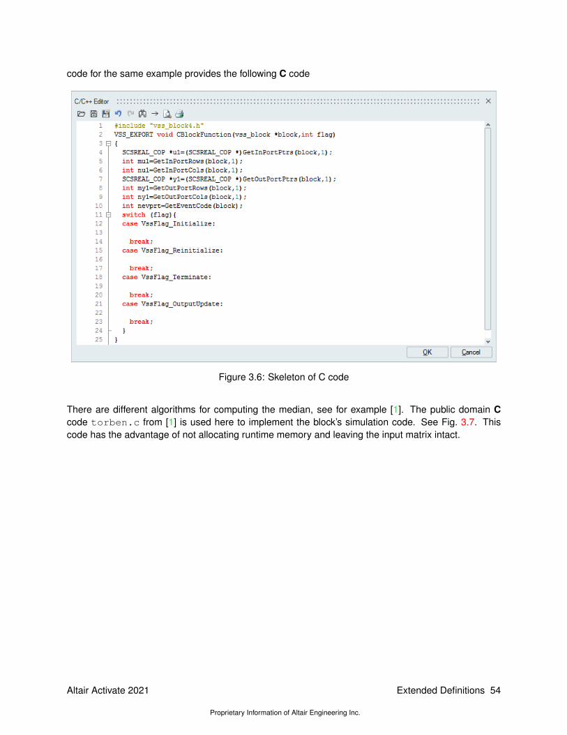
code for the same example provides the following C code
Figure 3.6: Skeleton of C code
There are different algorithms for computing the median, see for example [1]. The public domain Ccode torben.c from [1] is used here to implement the block’s simulation code. See Fig. 3.7. Thiscode has the advantage of not allocating runtime memory and leaving the input matrix intact.
Altair Activate 2021
Proprietary Information of Altair Engineering Inc.
Extended Definitions 54
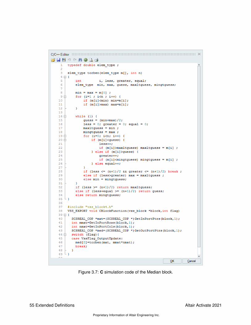
Figure 3.7: C simulation code of the Median block.
55 Extended Definitions
Proprietary Information of Altair Engineering Inc.
Altair Activate 2021

3.3.2 Variable discrete delay
A discrete delay block is considered where the amount of delay is variable and is given by an additionalblock input. Let u1 and u2 be the block inputs, then the output is given by
y(k) = u1(k − u2(k)),
The delay input u2(k) is supposed to be receive values between 1 and N . But if u2(k) is less than 1then the delay is set to 1; if it is larger than N then it is set to N .
The block is implemented using a circular buffer of size N placed in the discrete state z of the block.An integer state oz(1) is used to track the position of the last entry of z used to store the latest value ofthe input.
The CCustomBlock block is used to implement the Variable delay block. The block has two inputs. Forsimplicity, we assume both are scalars but the extension to vector case is straightforward. The first inputu1 is the delayed signal, which contrary to the second input representing the amount of delay, does nothave feedthrough property. See Fig. 3.8 for the parameterization of the ports of the CCustomBlockblock.
Figure 3.8: Parameterization of the ports of the Variable delay block.
The states are initialized as illustrated in Fig. 3.9. The buffer entries are initially set to zero and aninteger state is used to indicate the current position in the buffer.
The block has no parameters and the simulation code is given in Fig. 3.10.
The following model is used to test the Variable delay block:
Altair Activate 2021
Proprietary Information of Altair Engineering Inc.
Extended Definitions 56

Figure 3.9: Parameterization of the states of the Variable delay block.
Figure 3.11: Variable Delay model (delayVar.scm)
The simulation result is given in Fig. 3.12.
57 Extended Definitions
Proprietary Information of Altair Engineering Inc.
Altair Activate 2021

Figure 3.10: Parameterization of the states of the Variable delay block.
Figure 3.12: Simulation results show that the input signal is delayed differently at each step.
Altair Activate 2021
Proprietary Information of Altair Engineering Inc.
Extended Definitions 58

3.3.3 Fluid flow
The fluid flow between two tanks is modeled. The fluid levels in the tanks are denoted by h1 and h2satisfying the following equations:
h1 = −Ad
AtV
h2 =Ad
AtV
where V represents the speed of flow. At represents the cross-sectional areas of the tanks. Ad repre-sents the cross-sectional area of the pipe connecting the two tanks:
Ad =πD2
4(3.1)
where D is the diameter of the pipe.
The speed V satisfies the Bernoulli equation:
h1 +H = h2 + f2L
D
V 2
2g+V 2
2g
with H denoting the contribution of the pump. H = 0 if the pump is off; when the pump is on:
H = 4− 8.0×10⁴Q2. (3.2)
The flow Q is given by the equation of continuity:
Q = AdV. (3.3)
The friction factor f satisfies one of following relations depending on the flow phase: turbulent, laminaror transitional:
1√f
= −2 log10
(e
3.7+
2.51
Re√f
)if Re > ReT
f =Ks
Reif Re < ReL
f = fL +Re −ReL
ReT −ReL(fT − fL) Otherwise
The phase depends on the value of Re, the Reynold’s number:
Re =DV ρ
µ(3.4)
This system cannot be readily expressed as a system of ordinary differential equations and must bemodeled as an implicit system, i.e., a system of differential algebraic equations (DAE). Such systemsmay be modeled as Activate blocks, called implicit blocks. C and OML Custom Blocks can be used toimplement implicit blocks.
The difference between an explicit block and implicit block is that in an explicit block the continuous-timedynamical behavior is an explicit system
x = F (t, x, u)
y = G(t, x, u)
59 Extended Definitions
Proprietary Information of Altair Engineering Inc.
Altair Activate 2021

Here u and y represent respectively the inputs and the outputs of the block. The block simulation codeprovides the functions F and G.
The continuous-time dynamical behavior of an implicit block is
0 = E(t, x, x, u) (3.5)
y = H(t, x, x, u)
The block simulation code provides the functionsE andH . Unlike the explicit case where the simulationcode must compute x, in the implicit case the code computes a residual, which may depend on x.
Since algebraic relationships may be included in (3.5), it is possible to include all system equations in(3.5). In this case, the size of the state x (so the size of the residual) would be equal to the numberof equations in the system. But for better performance and precision, it is better to reduce the size ofresidual by computing explicitly system variables, when possible, and thus removing as many algebraicequations as possible. Here in particular instead of including Equations (3.1), (3.2), (3.3) and (3.4) in(3.5), Ad, H , Q and Re are computed explicitly and the state of the block is reduced to
x =
h1h2Vf
.
The C simulation code in CCustomBlock block for this example is given in Fig. 3.13.
All system parameters are defined as block parameters, so they can be modified without having to editthe C code. The block has one input (pump) taking values 0 and 1 indicating respectively that the pumpis off or on. The block outputs are the fluid levels in the tanks.
Note that in the CCustomBlock block parameter GUI, the Implicit block property checkbox must bechecked, the initial state specified and the Activation mode be set to Always Active mode.
The following model is used to test the two-tank block:
Figure 3.14: DrainingTanks C model (DrainingTanks_C.scm)
Altair Activate 2021
Proprietary Information of Altair Engineering Inc.
Extended Definitions 60

Figure 3.13: C simulation code of the two-tank block.
The pump may be turned on and off by double clicking on the Switch block. With the pump off, thesimulation stops when the fluid levels are equal and the simulation time is indicated in the Displayblock.
The simulation results for both the case the pump is on and off are given in Fig. 3.15:
61 Extended Definitions
Proprietary Information of Altair Engineering Inc.
Altair Activate 2021

Figure 3.15: Simulation results: h1 and h2 with pump off and on.
3.3.4 Simplified explicit automaton block
In chapter 16, the implementation of hybrid automata in Activate has been illustrated. The Automatonblock1 is an implicit block which allows modeling general hybrid automata with Differential algebraicequations (DAE). In this section we try to demonstrate the way a simplified Automation block for explicithybrid automata with ordinary differential equation (ODE) is built. The sticky balls example (16.3.3) willbe implemented using CCustomBlock block with the new explicit automation block.
As explained in (16.3.3), the sticky balls model works in two modes, stuck and separate. In each modethe dynamical model is described as an ODE of size four (see 16.11, 16.12, and 16.19). In order tosimulate the sticky balls models, the CCustomBlock block contains the state vector and outputs it. Thestate vector, in separate mode and stuck mode is [x1, x2, v1, v2] and [x3, v3, s, q], respectively. The blockoutputs the state vector at the second output port whatever the mode is. The derivative of the statesshould be computed as a function of states and given back to the CCustomBlock block as input. Thederivative of state in separate mode is fed to the first input and that of the stuck is given to the secondinput. During the mode transition, the initial value of state vector should be given to CCustomBlockblock to reinitialize the state vector. The initial value of states are concatenated with the state derivativeof the destination mode. In order to detect a mode transition, a zero-crossing function is used in eachmode. In the separate mode, the zero-crossing function in separate and stuck modes are 16.18 and16.20, respectively. The zero-crossing functions are concatenated with the state-derivative and initialvector for each mode. The overall model of the sticky balls are shown in Fig. 3.16.
The first output of the CCustomBlock block contains the current mode and the second output is thestate vector.
See Fig. 3.17 for the parameterization of the ports of the CCustomBlock block.
The states are initialized as illustrated in Fig. 3.9.
The block has two integer parameters, i.e., number of modes of the automaton, the initial mode. Thereare also two object parameters of type integer, i.e., the destination modes, when the zero-crossinghappens. In the case of sticky balls model, the destination modes is simple, when the mode is One,the destination mode when a zero-crossing happens, is Two and when the mode is Two the destinationmode is One. The parametrization is given in Fig. 3.19.
The number of zero-crossing function is one and the block has no internal mode for automatic handling
1Available in the Hybrid palette.
Altair Activate 2021
Proprietary Information of Altair Engineering Inc.
Extended Definitions 62

Figure 3.16: Complete model of sticky masses(Automat_StickyMasses_decay_ccustomblock_explicit.scm)
the zero-crossing. The C simulation code in CCustomBlock block for this example follows:#include "vss_block4.h"
typedef struct int cMode, pMode;automat_t;
#define WD ((automat_t *) GetWorkPtrs(block))#define _cMode (WD->cMode)#define _pMode (WD->pMode)
VSS_EXPORT void CBlockFunction(vss_block *block,int flag)double * y0, *y1, *ui;double* g=GetGPtrs(block);double* x=GetState(block);double* xd=GetDerState(block);double* evout= GetNevOutPtrs(block);
63 Extended Definitions
Proprietary Information of Altair Engineering Inc.
Altair Activate 2021

Figure 3.17: Parameterization of the ports of the explicit automaton block for sticky balls model.
int* ipar=GetIparPtrs(block);double* rpar=GetRparPtrs(block);int* jroot=GetJrootPtrs(block);int ng=GetNg(block);int NX=GetNstate(block);int* tmodev, NMode, Minitial,j,k;double time=GetVssTime(block);
NMode=ipar[0];Minitial=ipar[1];
switch(flag)case VssFlag_Initialize:if ((GetWorkPtrs(block)=(automat_t*) vss_malloc(block,sizeof(automat_t)))== NULL )
SetBlockError(block,1); return; _pMode=_cMode=Minitial;break;case VssFlag_OutputUpdate:y0=GetRealOutPortPtrs(block,1);y1=GetRealOutPortPtrs(block,2);y0[0]=(double) _cMode;
memcpy(y1,x,sizeof(double)*NX); y1+=NX;break;
case VssFlag_Derivatives:ui=GetRealInPortPtrs(block,_cMode);memcpy(xd,ui,sizeof(double)*NX);break;case VssFlag_ZeroCrossings:
Altair Activate 2021
Proprietary Information of Altair Engineering Inc.
Extended Definitions 64

Figure 3.18: Parameterization of the states of the explicit automaton block for sticky balls model.
ui=GetRealInPortPtrs(block,_cMode);for (j=0;j<ng;j++) g[j]=0;for (j=0;j<GetInPortRows(block,_cMode)-2*NX;j++) g[j]=ui[j+2*NX];break;
case VssFlag_StateUpdate:if (!( isZeroCrossing(block)
|| GetSimulationPhase(block)==PHASE_DISCRETE|| GetSimulationPhase(block)==PHASE_MESHPOINT )) return;
tmodev=Getint32OparPtrs(block,_cMode);ui=GetRealInPortPtrs(block,_cMode);
for (k=0;k<GetInPortRows(block,_cMode)-2*NX;k++)ui=GetRealInPortPtrs(block,_cMode);if( (isZeroCrossing(block) && jroot[k]==1) ||(GetNevIn(block)==1 && ui[k+2*NX]>0 ) ||(GetSimulationPhase(block)==PHASE_DISCRETE && ui[k+2*NX]>0) ||(GetSimulationPhase(block)==PHASE_MESHPOINT && ui[k+2*NX]>0)) _pMode=_cMode;_cMode=tmodev[k];
ui=GetRealInPortPtrs(block,_cMode);ui+=NX;memcpy(x,ui,sizeof(double)*NX);DoColdRestart(block);break;break;default:
65 Extended Definitions
Proprietary Information of Altair Engineering Inc.
Altair Activate 2021

Figure 3.19: Parameterization of the parameters of the explicit automaton block for sticky balls model.
break;
In order to hold the current and previous modes, they are put into a structure and stored in the block’sinternal workspace. The workspace is allocated and initialized in VssFlag_Initialize flag usingblock integer parameters.
In the VssFlag_OutputUpdate flag, the outputs are computed. The first output is straightforwardand in order to compute the second output, the state vector x=GetState(block) is copied into theoutput using the C memcpy command. The size of the state vector is obtained using nx=GetNstate(block).
In the VssFlag_Derivatives flag, first, based on the current mode _cMode the pointer to theappropriate input port is grabbed, then the first nx elements are copied into the state-derivative vector(xd=GetDerState(block)).
In the VssFlag_ZeroCrossings flag, first, based on the current mode _cMode the pointer to theappropriate input port is grabbed. The first 2nx elements of the input port are state derivative and initialvalue of states the next nz=GetNg(block) elements are the zero-crossing functions. Hence, theseelements are copied into the state-derivative vector (g=GetGPtrs(block)).
In the VssFlag_StateUpdate flag, the mode transition is performed. The mode can change atzero-crossing instants or at non-try simulator points such as discrete events or simulator meshpoints.At other instants, the call to the VssFlag_StateUpdate flag is ignored. If a valid transition happens,the zero-crossing surface of the next mode will be positive. Based on this, the positive zero-crossingis found and the corresponding mode is found. Then the internal state of the CCustomBlock block isupdated.
The simulation result of the model 3.16 is given in fig. 3.20.
Altair Activate 2021
Proprietary Information of Altair Engineering Inc.
Extended Definitions 66

Figure 3.20: Simulation result of the model 3.16.
3.4 Non-inlined simulation functions
The C and OML functions used in custom blocks need not necessarily be provided in the block (beinlined). They can be provided in a shared library (dll file under Windows) for CCustomBlock blocks orOML files for OmlCustomBlock blocks. The choice of inlining the function is made using a checkboxin the SimFunction tab. For example in Fig. 3.21 the simulation function of the CCustomBlock blockis defined in the file foolib.dll. Since the path of the file is not specified, the file is supposed be in thesame directory as the model.
Figure 3.21: SimFunction tab used to specify the simulation function. In this case the function is notinlined.
A convenient way to create a CCustomBlock block without inlined code is first to create one withan inlined code. This way, the skeleton generator facility can be used and the code can be tested.
67 Extended Definitions
Proprietary Information of Altair Engineering Inc.
Altair Activate 2021

Moreover, the shared library is automatically created by Activate. Once the code is validated, theblock may use the shared library instead of the inlined code. This can be done automatically using theconvert to non inlined facility. In this case the inlined checkbox is unchecked and the library informationis provided in the SimFunction tab. Note that the “Function code” becomes an invisible parameter butits content, the original C code, can be retrieved by marking the inlined checkbox. So if the objective isto hide the code (in particular for IP protection), make sure to erase the content of the “Function code”parameter.
If the shared library of the non-inlined CCustomBlock block has dependency on other shared libraries,then the location of these libraries must be provided. These libraries may include both external dll filesthat must accompany the model and Activate dll files already available in the software distribution. Inparticular if the CCustomBlock block is created using the Activate code generation facility, the librariesassociated with the blocks used in the diagram are included in the list of libraries.
Altair Activate 2021
Proprietary Information of Altair Engineering Inc.
Extended Definitions 68

Bibliography
[1] Nicolas Devillard, Fast median search: an ANSI C implementation, 1998.http://ndevilla.free.fr/median/median/.
69 Extended Definitions
Proprietary Information of Altair Engineering Inc.
Altair Activate 2021

Altair Activate 2021
Proprietary Information of Altair Engineering Inc.
Extended Definitions 70

Chapter 4
Simulation restarts: implementingiterations
In some applications, a single time simulation does not provide a solution to the problem. This isparticularly the case where multiple simulations are needed to solve problems such as parameter fitting,solving nonlinear systems, optimizing, etc. Time simulation iterations in Activate are implementedthrough the End block, which can either stop the simulation for good, or stop and restart a new timesimulation. These actions are controlled by activation signals in Activate.
Activation signals represent the key element in Activate formalism. They determine in particular when,how and in what order the block simulation functions are called during simulation. The ability to ex-plicitly manipulate Activation signals, gives users modeling capabilities that are seldom present in othermodeling and simulation tools.
The use of Activation signals go beyond the framework of a single simulation run. Within the formalismof Activate, there exists the possibility of creating models where their simulations lead to multiple timesimulations. Indeed in Activate an activation signal can end or restart a time simulation. This ability toconditionally restart simulations is particularly useful for parameter optimization, strategy assessment,Monte Carlo simulation, etc. Traditionally, such applications are developed using scripts calling thesimulator in batch mode. By integrating the complete formulation within the simulation model (whichactually is a misnomer since the model contains more than a simulation model), the implementationbecomes more concise and easy to maintain. There is of course always the possibility to use OMLscripts to code the optimization part and run Activate simulations in batch mode.
To illustrate possible applications of conditional restart in Activate, an example is presented here. Inparticular the implementation of the shooting method for solving boundary value systems is considered.Boundary value systems are for example obtained when solving trajectory optimization problems. Aboundary value system is often a system of ODEs defined over a time interval [Ti, Tf] where the statesof the system are not fully specified at the initial time of the interval. The problem is well posed thanksto conditions specified on the states at the final time of the interval.
The simplest implementation of the shooting method for solving boundary value systems consists ofguessing values for the missing states of the system at initial time, simulating the system up to the finaltime, comparing the final states with the constraints imposed on them and based on this comparisongenerate new guess values for the initial states. The iterations are continued until the final states satisfythe constraints up to desired precision.
71 Extended Definitions
Proprietary Information of Altair Engineering Inc.
Altair Activate 2021

To implement the shooting method in Activate, it is then necessary to model the system and implementa mechanism to compute new guess values and, until the desired precision is not achieved, to restartthe simulation after changing the initial conditions. The system modeling is done as usual without anyspecial consideration for the shooting method. The system model should provide a function of the finalstate of the system representing the constraints (the value of the function is zero if the constraints aresatisfied).
For well-posed boundary value problems, the number of free initial states is equal to the number of finalconstraints. Let p denote the subset of initial state which are free and f the final constraint function,i.e.,
f(x(Tf)) = 0 (4.1)
where x represents the states of the system. The final state x(Tf) depends of course on the initial statex(Ti) and in particular on p: x(Tf) = H(Tf, p). The function H can only be evaluated numerically bysimulating the system from Ti to Tf. For a given Tf, the constraint (4.1) can be expressed as
f(x(Tf)) = f(H(Tf, p)) = g(p) = 0.
The solution p of the nonlinear system g(p) = 0, which has as many equations as unknowns, canbe obtained using various methods. For example the OML function fsolve is provided specificallyfor solving such problems. This function can be used in an OML script to solve the boundary valueproblem by running the simulation model programmatically. THe objective however here is to includethe solution of the problem within the model, obtaining a self contained formulation of the problem interms of an Activate diagram without any dependency on external code. So a nonlinear solver similarto fsolve must be made available in Activate, as a block.
4.1 Nonlinear solver block
A nonlinear solver block cannot function the way fsolve does. In fsolve, the nonlinear solveriterates by calling an external function provided by the user evaluating the function g(p) for the given puntil an end condition is satisfied, in which case the function returns the solution p, or an error message.fsolve is the main and the function evaluating g(p) the secondary. This main-secondary configurationis not appropriate for implementing a solver block in Activate. In Activate, the Activate simulator is themain solver and the blocks are secondary elements. For that, the solver algorithm must be implementedin reverse-communication mode. Many nonlinear solver and optimization codes are available both innormal and reverse-communication modes.
4.1.1 A reverse-communication solver
In reverse-communication mode, the solver is provided with the values of p and g(p) and returns a newvalue of p indicating also whether this value is the solution or a value to be used for the next iteration.If we make the assumption that the main solver calls back systematically the solver function with pprovided by solver at the previous iteration, then it is fairly straightforward to reprogram any solver inreverse-communication mode. The structure of the program must be changed so that the internal stateof the solver is maintained from one call to the next. The solver algorithm however is not modified.
If the solver function is not recalled with the value it returns, then specific reverse-communication al-gorithms are required. This is the case considered here for the implementation of a nonlinear solver
Altair Activate 2021
Proprietary Information of Altair Engineering Inc.
Extended Definitions 72

block. The function used here is a simple nonlinear solver implemented as toy code to illustrate theapproach. The internal state of the function contains a number of previous (p, g(p)) pairs and a weightfunction associated with each one. At each iteration, the new pair (p, g(p)) replaces the “least inter-esting” (having the smallest weight) pair and the eights are updated. The weight associated to a pair(p, g(p)) depends on the norm of g(p) and how long ago the pair has been received. The weight isreduced at every iteration.
Let p be close to the solution p∗ satisfying g(p∗) = 0), then by neglecting higher order terms,
g(p) = −J(p− p∗) (4.2)
where J = ∂g∂p(p∗) is the Jacobian matrix. This relation is the basis of the Newton’s method when J is
known. Using this relation for the pairs (pi, g(pi)), i = 1, · · · , N , yields
p∗ = pi − J−1g(pi), i = 1, · · · , N. (4.3)
The unknowns are p∗ and J so the system has enough equations if N = n + 1 where n is the size ofp, and it is over-determined if N > n + 1. In this latter case, a least-squared problem is formulated asfollows
p∗ = pi − J−1g(pi) + vi, i = 1, · · · , N, (4.4)
with a cost function to minimize:
J =N∑i=1
wi‖vi‖2. (4.5)
w−1i ’s are weights associated with each equation.
The set of equations (4.4) can be expressed in matrix form as follows
p∗T = P − J−1G+ V (4.6)
whereT =
[1 1 · · · 1
], P =
[p1 p2 · · · pN
]and
V =[v1 v2 · · · vN
], G =
[g(p1) g(p2) · · · g(pN )
].
.
The value of interest here is p∗, so the matrix J can be removed from the system by multiplying (4.6)on the right by G⊥, a maximum rank right-annihilator of G:
p∗TG⊥ = PG⊥ + V G⊥ (4.7)
which can be expressed asAp∗ = b+ Cν (4.8)
where A = (TG⊥)T ⊗ I,1 b is the vector obtained by concatenating the columns of the matrix PG⊥
and C = (G⊥)T ⊗ I. The vector ν is obtained by concatenating the vi’s.
The cost J in (4.5) can be expressed as follows
J = νTWν (4.9)
1The ⊗ operation represents the Kronecker product.
73 Extended Definitions
Proprietary Information of Altair Engineering Inc.
Altair Activate 2021

where
W =
w1I
w2I· · ·
wNI
.The solution p∗ minimizing J in (4.9) subject to (4.8) satisfies
[A −CTW−1C0 AT
] [p∗
λ
]=
[b0
]
from which the solution can be explicitly obtained as follows
p∗ =[I 0
] [A −CTW−1C0 AT
]−1 [b0
].
This algorithm can be coded as an OML function as follows:
function [pnext,TT]=nsolve(p,gp,TT)n=length(p);N=size(TT,2);G=TT(1:n,:);P=TT(1+n:2*n,:);wi=TT(2*n+1,:);wi=wi*(1+1/n);[_x,idx]=max(wi);G(:,idx)=gp;P(:,idx)=p;wi(idx)=gp’*gp;[Q,R]=qr(G’);r=rank(R);Gperp=Q*[zeros(N-r,r);eye(r)];At=ones(1,N)*Gperp;Bt=P*Gperp;Ct=Gperp;A=kron(At’,eye(n));b=Bt(:);C=kron(Ct’,eye(n));Wi=kron(diag(wi),eye(n));m=size(A,1);pnext=[eye(n),zeros(n,m)]*...
inv([A,-C*Wi*C’;zeros(n,n),A’])*[b;zeros(n,1)];if norm(p-pnext)<eps
pnext=pnext+2*eps*rand(n,1);endTT=[G;P;wi];
end
The arguments of the function are p, the value of g(p) and a matrix _TT used as as internal state of thefunction used to store the previous values of p, g(p) and the associated weights (more specifically theinverse of the weight).
The function returns a new value of p to be used at the next iteration and the updated internal statematrix _TT. This matrix could be initialized and retained by the function itself (and not be part of its inputoutput arguments) from one call to the next be defining it as persistent. In the way this function willbe used in the construction of a Activate block, it is easier to have the calling function keep the valueof _TT.
The stopping tests based the value of g(p) and the maximum number of iterations are not implementedin this function and are handled externally.
Altair Activate 2021
Proprietary Information of Altair Engineering Inc.
Extended Definitions 74

4.1.2 Activate block implementation
The nonlinear solver block is implemented as a Super Block where the central piece is an OmlCus-tomBlock block implementing the solver function nsolve developed in the previous section. Thisblock has 3 regular inputs and 2 regular outputs corresponding to the arguments of nsolve. It alsohas an activation input port for its activation.
The Super Block should also implement the logic to stop the iterations and propose a user friendlyinterface for the user. The block is shown in Fig. 4.1. The block is a Super Block, with 2 inputs and 3outputs: the inputs correspond to the pairs (p, g(p)) and the outputs are the new value of p proposedfor iteration, a stop signal set to 1 if no further iterations are required and finally an error output, set to1 if the iterations should stop on an error (the number of iterations exceeding the maximum allowed).
The block is masked as shown in Fig. 4.2. The parameters ftol, maxiter, sz are used to pa-rameterize the solver. The last parameter, count, may be made invisible; the value of the variable__counter__ corresponds to the iteration number; the first iteration is numbered one.
Figure 4.1: The new nonlinear solver block.
Figure 4.2: The mask of the Super Block.
The content of the Super Block is shown in Fig. 4.3. And its Context contains the following script
if count==1n=prod(sz);N=2*n;G=[eye(n,n),eye(n,n)];G=G(:,1:N);P=[eye(n,n),eye(n,n)];P=P(:,1:N);wi=ones(1,N)*1e32;TT=[G;P;wi];
elseTT=GetFromBase(’_TT’,[]);
end
So at the first iteration, the value of TT is initialized in the Context. In the subsequent iterations, thevalue is read from the Base environment, in particular the variable _TT. This is done thanks to theOML function GetFromeBase. The second argument of this function is optional and is used onlyif the variable named in the first argument does not exist in the Base environment. In this case, thevariable _TT exists at the second iteration because it has been defined by the block ToBase blockin the diagram. Variables in the Base environment are used to hold and pass values from one time
75 Extended Definitions
Proprietary Information of Altair Engineering Inc.
Altair Activate 2021
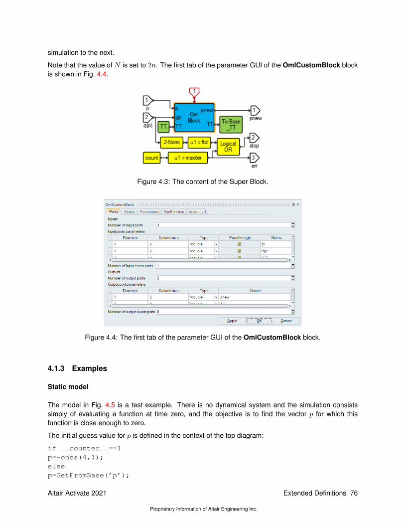
simulation to the next.
Note that the value of N is set to 2n. The first tab of the parameter GUI of the OmlCustomBlock blockis shown in Fig. 4.4.
Figure 4.3: The content of the Super Block.
Figure 4.4: The first tab of the parameter GUI of the OmlCustomBlock block.
4.1.3 Examples
Static model
The model in Fig. 4.5 is a test example. There is no dynamical system and the simulation consistssimply of evaluating a function at time zero, and the objective is to find the vector p for which thisfunction is close enough to zero.
The initial guess value for p is defined in the context of the top diagram:
if __counter__==1p=-ones(4,1);elsep=GetFromBase(’p’);
Altair Activate 2021
Proprietary Information of Altair Engineering Inc.
Extended Definitions 76

end
The variable __counter__ is provided by the system and represents the number of times the timesimulation is performed. At the first iteration, the value of p is initialized in the Context. In the subsequentiterations, the value is read from the Base environment, in particular the variable p. This is done thanksto the OML function GetFromeBase. The variable exists at the second iteration because it has beendefined by the block ToBase in the model.
The time simulation restarts when the End block with option Restart is activated. This block is activatedat the event at time zero only if the start signal has value zero. The simulation is no longer restartedif start has value 1, in which case depending on the value of the signal err, the simulation ends with asuccess message or an error message.
The use of Base variables and simulation restarts will be further explored when discussing optimizationin the Chapter 6.
Shooting model
This example corresponds literally to a shooting problem. Projectile is fired with a given initial velocityV and the objective is to find the firing angle so that the projectile lands at a distance d.
Denoting the position and the velocity of the projectile in 2D by s = (x, y) and v = (vx, vy), theequations of motion are given by
s = v, x(0) = 0,
v = −α(|v|β−1)v +
[0−g
], v(0) =
[cos(θ)sin(θ)
]V.
The problem is then finding the initial firing angle θ such that when y crosses zero, x is close to d. Sothe nonlinear function to solve is f(θ) = x − d. The problem is formulated as an Activate model inFig. 4.6. The system parameters are defined in the Initialization script of the model:
a=.1;b=2.5;g=9.8;V=1000;d=9;
and the initial guess value of θ is defined in the Context:
if __counter__==1p=pi/3;elsep=GetFromBase(’p’);end
77 Extended Definitions
Proprietary Information of Altair Engineering Inc.
Altair Activate 2021

Figure 4.5: The End block is used in different configurations to restart the simulation, stop it with asuccess message and stop it with an error.
Altair Activate 2021
Proprietary Information of Altair Engineering Inc.
Extended Definitions 78

Figure 4.6: The implementation of the shooting method. In this case the final simulation time is notfixed and is determined by the time of the zero-crossing detected by the ZeroCrossDown block.
79 Extended Definitions
Proprietary Information of Altair Engineering Inc.
Altair Activate 2021

4.1.4 Solving nonlinear system without a specific block
The new nonlinear solver block is convenient to use for solving nonlinear systems in Activate butthe iterative method presented in the previous sections can be implemented without it. The functionnsolve introduced earlier can be used directly in the Context of the diagram, as it is shown below.The Model in Fig. 4.7 is an alternative implementation of the model in Fig. 4.6. Assuming the file
Figure 4.7: The implementation of the shooting method without using a specific block.
defining nsolve is in the path, the solver part is implemented in the Context of the diagram as follows:
if __counter__==1n=length(p0);N=2*n;G=[eye(n,n),eye(n,n)];G=G(:,1:N);P=[eye(n,n),eye(n,n)];P=P(:,1:N);wi=ones(1,N)*1e32;TT=[G;P;wi];p=p0;
elseTT=GetFromBase(’_TT’,[]);p=GetFromBase(’_p’,[]);gp=GetFromBase(’_gp’,[]);if norm(gp)<1e-5
printf(’succesfull convergence, p=%g, g(p)=%g’,p,gp);return
end[p,TT]=nsolve(p,gp,TT);if __counter__>100
error(’Max nb. of iterations reached.’);end
endAddToBase(’_p’,p);AddToBase(’_TT’,TT);
Altair Activate 2021
Proprietary Information of Altair Engineering Inc.
Extended Definitions 80

Example
The problem considered here is an optimal control problem where the objective is to find a functionoptimizing a cost function. The example consists of the computation of geodesics for the Grusin’smetric. See [1] for details. The problem considered here is the following:
J = min
∫ 1
0u21 + u22 dt
subject to
x1 = u1 (4.10)
x2 = u2x1 (4.11)
with boundary conditions x1(0) = x2(0) = x1(1) = 0 and x2(1) = 1/(2π).
The Lagrangian is defined as follows
L =1
2(u21 + u22) + λ(x1 − u1) + µ(x2 − u2x1)
from which the following optimality conditions are obtained
λ = −µ2x1 (4.12)
µ = 0 (4.13)
with optimal controls u1 = λ and u2 = µx1.
This system can be solved analytically but here it is used to illustrate the usage of the shooting method.Since µ is a constant, the unknowns are considered to be p = (λ(0), µ) and the system of equations tosolve is
g(p) =
[x1(1)
x2(1)− 1/(2π)
]where x1(1) and x2(1) are obtained by integrating the system
x1 = λ
x2 = µx21
λ = −µ2x1
with initial conditions x1(0) = x2(0) = 0. These equations are obtained from (4.10), (4.11), (4.12) andusing the optimal controls u1 = λ and u2 = µx1.
The solution is implemented as the Activate model in The Initialization script defines the final conditionsof x and an initial guess for the unknown p:
xT=[0;1/(2*pi)];p0=[1;1];
The Context is the following script:
n=length(p0);N=2*n;if __counter__==1
81 Extended Definitions
Proprietary Information of Altair Engineering Inc.
Altair Activate 2021

Figure 4.8: Model implementing the computation of geodesics for the Grusin’s metric.
done=false;G=[eye(n,n),eye(n,n),eye(n,n)];G=G(:,1:N);P=[eye(n,n),eye(n,n),eye(n,n)];P=P(:,1:N);wi=ones(1,N)*1e32;TT=[G;P;wi];p=p0;
elseTT=GetFromBase(’_TT’,[]);p=GetFromBase(’_p’,[]);gp=GetFromBase(’_gp’,[]);if norm(gp)<1e-5
printf(’succesfull convergence, p=%g, g(p)=%g’,p,gp);done=true;
elseif __counter__>100error(’Max nb. of iterations reached.’);
elsedone=false;[pn,TT]=nsolve(p,gp,TT);
al=(__counter__<=N)*0.9;p=al*p+(1-al)*pn;end
endAddToBase(’_p’,p);AddToBase(’_TT’,TT);
The simulation resutls are shown in Fig. 4.9 and 4.10.
Altair Activate 2021
Proprietary Information of Altair Engineering Inc.
Extended Definitions 82

Figure 4.9: Optimal solution x1 versus x2.
Figure 4.10: Optimal controls.
4.2 Repeating activations
The RepeatActivation block in Activate can be used to implement iterative computations at singleevent times. A simple example is presented to show its usage. In particular, the computation of thesolution of a nonlinear equation is implemented using the Newton’s method.
The RepeatActivation block plays also an important role in the implementation of state machines inActivate.
83 Extended Definitions
Proprietary Information of Altair Engineering Inc.
Altair Activate 2021

4.2.1 Problem setup
The problem considered here is a 2D version of a ball bouncing on a not-necessarily-flat surface. Thesurface is defined by a curve
y = f(x). (4.14)
User defines the function f and its derivative f ′. The ball is supposed to be a point-mass, and thecollision with the surface elsastic.
The objective is to model and simulate this system in Activate.
4.2.2 System equations
The state of the system contains the position (x, y) and the velocity (w, v) of the ball. The ball is subjectto gravity, so its movement can be expressed as follows
x = w (4.15a)
w = 0 (4.15b)
y = v (4.15c)
v = −g. (4.15d)
The collisions occur when (x, y) hits the curve, i.e, when (4.14) is satisfied.
The collision of the ball with the surface creates a jump in the velocity of the ball. The new velocitycan be obtained using the law of conservation of momentum and the assumption of the conservationof energy (elastic collision), resulting in the following(
wv
)←(
1 f ′(x)−f ′(x) 1
)−1(1 f ′(x)
f ′(x) −1
)(wv
).
For this particularly simple example, it is possible to explicitly solve the differential equations. Given thecurrent position and velocities of the ball, its new position and velocity, t seconds in the future, assumingno collisions occur during this period, can be expressed as follows
w ← w
v ← v − gtx ← x+ wt
y ← y + vt− 1
2gt2.
The time delay t is the time to the next collision. So t is the smallest positive value satisfying
h(t) , y + vt− 1
2gt2 − f(x+ wt) = 0. (4.16)
The solution to this nonlinear equation is obtained using Newton’s iterations
tk+1 = tk −h(tk)
h′(tk). (4.17)
The iterations are ended when |h(tk)| falls below a given threshold. The function h′(t) can be expressedas follows
h′(t) = v − gt− f ′(x+ wt)w. (4.18)
Altair Activate 2021
Proprietary Information of Altair Engineering Inc.
Extended Definitions 84

Figure 4.11: Atomic super block, next time, implementing the Newton iterations (4.17).
4.2.3 Implementation in Activate
The implementation of the Newton iterations (4.17) is realized using a RepeatActivation block. Whenthis block is activated by an event, once all the blocks activated by this event are processed, the sameevent is re-activated. This is done at the same synchronous time instant. For the rest of the model, theresult of all the iterations are seen as a single event activation. The re-activated event is the primaryevent associated with the event that activated the RepeatActivation block. To confine the re-activationto the desired area of the model, it is convenient to use an Atomic super block. The implementation ofthe Newton iterations (4.17) can be seen in Figure 4.11.
The top diagram of the model ball_bounce_.scm is shown in Figure 4.12. For the sake of animation,the next event time is considered to be the minimum of the next collision time and a constant time stepdt.
Note that the objective here has been to illustrate the use of the RepeatActivation block. The modelis a naive implementation. For example the next collision time is computed at every dt; this can beoptimized. And there is no guarantee that the Newton’s iterations converge to a positive solution. Sothe simulation may fail for some surfaces y = f(x).
85 Extended Definitions
Proprietary Information of Altair Engineering Inc.
Altair Activate 2021

Figure 4.12: Top diagram of the model.
Altair Activate 2021
Proprietary Information of Altair Engineering Inc.
Extended Definitions 86

Bibliography
[1] Ugo Boscain and Benedetto Piccoli, “An introduction to optimal control” in ContrôleNon Linéaire et Applications, January 2005. http://www.cmapx.polytechnique.fr/~boscain/AUTOMATICS/introduction-to-optimal-control.pdf
87

Altair Activate 2021
Proprietary Information of Altair Engineering Inc.
Extended Definitions 88

Chapter 5
Example: Implementation of an ExtendedKalman Filter in Activate
Kalman filter is an algorithm that uses several measurements which are polluted by noise and producesestimates of the unknown signal. The estimated signal tends to be more precise than those based ona single measurement. The Kalman filter has numerous applications and is a widely applied conceptin time series analysis used in fields such as signal processing, navigation and econometrics. Theextended Kalman filter (EKF) is the nonlinear version of the Kalman filter which linearizes about anestimate of the current mean and covariance. In the case of well defined transition models, the ex-tended Kalman filter is the de-facto method of state estimation for non-linear systems. This techniqueessentially linearizes a non-linear system at an operating point to be able to use the linear Kalman Filtermethods of state estimation.
In this chapter, the implementation of an Extended Kalman Filter (EKF) in Activate is illustrated throughan example. The problem considered has been presented in [1]. It consists of constructing an estimatorfor the airspeed of a projectile using the measurements of its axial acceleration. The dynamics ofthe projectile is modeled as a system of nonlinear differential equations and noisy observations aresupposed to be available periodically. The estimator is implemented using an EKF.
The model of the projectile is the following:
Vzθ
= f
Vzθ
=
1
2mρV 2SrefCd − g sin(θ)
−V sin(θ)
− gV
cos(θ)
where the model states V , z and θ are air-relative speed, altitude, and angle of attack of the projectilerespectively. The model parameters m, ρ, Sref, Cd, and g are the projectile mass, the air density, thereference surface of the projectile, the drag coefficient, and the gravity acceleration respectively. Thesensor provides the axial acceleration of the projectile. Thus the measurement equation used as themeasurement equation of the Kalman filter is:
h(V, z) = ax =1
2mρV 2SrefCd.
The value of Cd is usually provided through a table as a function of the Mach number M . Here theMach number is given by the formula M = V/a where a is the speed of sound. The speed of sound is
89 Extended Definitions
Proprietary Information of Altair Engineering Inc.
Altair Activate 2021

a function of the air density ρ, which in turn is given by the following empirical equation given in [2]:
ρ(z) = (ρ0 + 0.00651z
T0)4.256 (5.1)
where ρ0 and T0 represent the air density and air temperature at see level.
5.1 Activate model
Figure 5.1: Projectile speed estimation model (Hybrid_Extended_Kalman_Filter.scm)
The above model is implemented in Activate as illustrated in Figure 5.1. This diagram contains thewhole system including the projectile model and the EKF. The parameters of the model are defined inthe Context of the diagram as shown in Figure 5.2:
In the Context Editor of Activate, the projectile parameters, the drag coefficient of the projectile as a
function of the Mach number Cd(M) as well as expressions for its derivativedCddM
are given. In the
projectile model, in order to compute the Mach number, the air density and the sound speed are firstcomputed as a function of altitude and the projectile speed. These values are computed using twoMathExression blocks. Once the Mach number is computed, a lookup table is used to find out thedrag coefficient of the projectile. Two noise sources with Normal distribution are used to simulate theprocess and the measurement noises. The Covariance of theses sources are defined in the contexteditor.
Altair Activate 2021
Proprietary Information of Altair Engineering Inc.
Extended Definitions 90
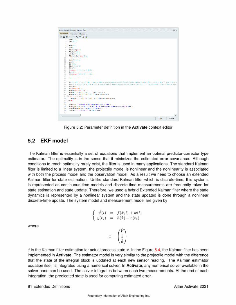
Figure 5.2: Parameter definition in the Activate context editor
5.2 EKF model
The Kalman filter is essentially a set of equations that implement an optimal predictor-corrector typeestimator. The optimality is in the sense that it minimizes the estimated error covariance. Althoughconditions to reach optimality rarely exist, the filter is used in many applications. The standard Kalmanfilter is limited to a linear system, the projectile model is nonlinear and the nonlinearity is associatedwith both the process model and the observation model. As a result we need to choose an extendedKalman filter for state estimation. Unlike standard Kalman filter which is discrete-time, this systemsis represented as continuous-time models and discrete-time measurements are frequently taken forstate estimation and state update. Therefore, we used a hybrid Extended Kalman filter where the statedynamics is represented by a nonlinear system and the state updated is done through a nonlineardiscrete-time update. The system model and measurement model are given by
˙x(t) = f(x, t) + w(t)y(tk) = h(x) + v(tk)
where
x =
Vzθ
x is the Kalman filter estimation for actual process state x. In the Figure 5.4, the Kalman filter has beenimplemented in Activate. The estimator model is very similar to the projectile model with the differencethat the state of the integral block is updated at each new sensor reading. The Kalman estimatorequation itself is integrated using a numerical solver. In Activate, any numerical solver available in thesolver pane can be used. The solver integrates between each two measurements. At the end of eachintegration, the predicated state is used for computing estimated error.
91 Extended Definitions
Proprietary Information of Altair Engineering Inc.
Altair Activate 2021

Figure 5.3: Model of the projectile
5.3 Covariance prediction
In Kalman filter the error covariance matrix (P ) containing the filter’s estimated error covariance for theKalman states (x). The following relationship defines the way this matrix is evaluated as a function ofthe system Jacobian (A) and process noise (Q).
P = AP + PAT +Q
The system process noise is a way to tell the filter how much the system dynamic model should betrusted. The system Jacobian matrix A is the partial derivative of f(x) with respect to x. In computing
the matrix A(x), we need to compute∂Cd∂z
and∂Cd∂V
. These two values can be computed as follows:
∂Cd∂V
=∂Cd∂M
∂M
∂V
∂Cd∂z
=∂Cd∂M
∂M
∂z
∂Cd∂M
is a table as a function of M whose values are be computed by brute force differentiating of the
table CX(M). The value of∂M
∂Vis simply
1
a, where a is the speed of the sound. The value of
∂M
∂zis however more tricky to compute. The sound speed (a) as a function of air density (ρ), see levelair-speed (a0), and see level air density (ρ0) is given by
a = a0
√ρ
ρ0
Altair Activate 2021
Proprietary Information of Altair Engineering Inc.
Extended Definitions 92

Thus, we can get∂M
∂z= − V
a2∂a
∂z= − V a0
2a2√ρρ0
∂ρ
∂z
The value of∂ρ
∂zcan be obtained by differentiating equation (5.1) with respect to z. The computation of
these values in Activate are illustrated in Figure 5.6.
Figure 5.4: Kalman estimator
5.4 State update
At each sensor observation (an event activation in Activate), the a posteriori Kalman state andthe error covariance state are updated with the following relation:
x+ = x− +K(ameasurement − h(x−))P+ = (I −KH)P−
where ameasurement is the measured value at tk. The gain K is computed as follows:
K = P−HT (HP−HT +R)−1
where H =∂h(x)
∂x. In Figure 5.5, the implementation of the error covariance matrix and the state
update computation in Activate are illustrated.
93 Extended Definitions
Proprietary Information of Altair Engineering Inc.
Altair Activate 2021

Figure 5.5: Kalman state and error covariance state Update
5.5 Simulation
In Figure 5.7 the actual process states (in red) as well as the Kalman estimation of the states are shown.In Figure 5.8, the Kalman estimation error is shown.
Altair Activate 2021
Proprietary Information of Altair Engineering Inc.
Extended Definitions 94
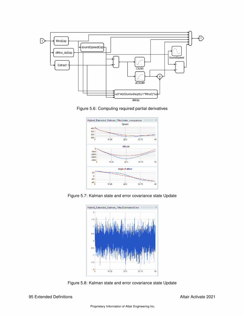
Figure 5.6: Computing required partial derivatives
Figure 5.7: Kalman state and error covariance state Update
Figure 5.8: Kalman state and error covariance state Update
95 Extended Definitions
Proprietary Information of Altair Engineering Inc.
Altair Activate 2021

Altair Activate 2021
Proprietary Information of Altair Engineering Inc.
Extended Definitions 96
Bibliography
[1] Thomas Recchia, Projectile velocity estimation using aerodynamics and accelerometer measure-ments: a kalman filter approach, US Army research center, New Jersey, 2010.
[2] Barnes W. McCormick, Aerodynamics Aeronautics and Flight Mechanics. 2nd ed., John Wiley &Sons, Inc., New York, NY, 1995.
97 Extended Definitions
Proprietary Information of Altair Engineering Inc.
Altair Activate 2021

Altair Activate 2021
Proprietary Information of Altair Engineering Inc.
Extended Definitions 98

Chapter 6
Optimization
In many applications, modeling and simulation are used to find optimal values for system parametersor optimal control strategies. This can be done by formulating an optimization problem with propercost function associated with the simulation model. There are various ways to define and solve suchoptimization problems in Activate. This document describes some of the available methods.
The outline of this chapter is as follows: first the Optimization block is presented. This block may beused to formulate optimization problems fully integrated within Activate models. Then batch simulationfrom the OML environment is presented and its application to optimization is illustrated via severalexamples. Finally, a graphical tool specifically developed for optimization in Activate is presented. Thegraphical tool is probably the simplest way to formulate and solve optimization problems in Activate butunderstanding its operations requires some knowledge of batch simulation that is why it is presentedlast.
6.1 Use of Optimization block in Activate
The Optimization (BobyqaOpt) block, available in the Optimization palette, may be used to solveoptimization problems using the BOBYQA software written by Prof. Powell, implemented in reversecommunication mode.
Figure 6.1: BOBYQA block
Unlike the usual optimization procedures where the optimization code is the main code calling thesimulator for cost evaluation by providing the value of the variable, in reverse communication mode thesimulator runs the main program and calls the optimizer with the cost value. The optimizer then returnsa new value of the variable indicating whether the optimization should be continued or that this valuecorresponds to the optimal value of the variable.
The Optimization block parameters are the optimization parameters and the inputs and outputs of theblock are used to exchange variable values (vectors in general), cost and control signals between the
99 Extended Definitions
Proprietary Information of Altair Engineering Inc.
Altair Activate 2021

optimizer and the simulator. The block restarts the simulation as long as necessary until the optimalsolution is found.
This method requires a way to maintain the value of the optimization variable from one simulation runto the next. This may be done using the ToBase and FromBase blocks. The ToBase block, whenactivated, copies the value of its input into a variable in the base OML workspace. The name of thevariable is given by the block parameter. The FromBase block, when activated does the opposite: itcopies the value of the variable to its output. If the variable name specified by the FromBase blockparameter does not exist in the base OML workspace, a default value is copied.
The first input of the Optimization block is used to pass the initial/current value of the variable tothe optimizer. The second input is used to pass the cost associated with the value produced by theOptimization block on its first output in the previous simulation run. The block is activated when anew value of the cost is available, usually at the end of every simulation run. The block then producesthe optimization variable on its first output, and either restarts the simulation or generates an eventindicating that the optimization has ended and that the variable provided on the output is the solution tothe optimization problem. In general the activation output is connected to an End block with parameter“Stop” but other configurations are possible. The optimal cost is provided by the second output of theblock.
6.2 Example
The following is a simple example to illustrate the use of the Optimization block. The problem consid-ered is that of finding the optimal gear ratios for a 5 speed vehicle given its torque curve as a functionthe engine RPM. This should be considered a toy example: the model is very simple and in particulardoes not consider the clutch mechanism. Multiple optimization criteria will be examined.
The simple model used for the dynamics of the vehicle is given by the following equations:
ω = g2i T (ω)q/c− aω − bv2
v = cω/gi
x = v.
The variable ω designates the engine angular velocity, gi is the gear ratio for gear number i, v is thespeed of the vehicle and x the traveled distance. T (ω) is the torque as a function of the angular velocity,and a and b are constant friction coefficients. q and c are also constant coefficients depending on vehiclecharacteristics. At the time of gear shift, ω jumps so that v remains a continuous-time function. Thesystem is modeled as a Super Block named car the content of which is illustrated in Fig. 6.2.
The 5 activation links entering the diagram on the top are used to model the shifting events; the Selectorblock outputs the corresponding gear ratio. The Torque curve is modeled using a Lookup table block.
The first optimization problem consists of finding the maximum traveled distance in 30 seconds startingwith a given small initial speed. The optimization variables are the gear ratios and the shift times. Eventhough given the gear ratios it is possible to find the up-shift times without optimization in this simplecase, we consider them as optimization variables for simplicity. So there are 9 optimization variables: avector T of size 4 representing the time lapses from one up-shift to the next, and a vector gear of size5 that represents the gear ratios associated with the gearbox.
The Optimization block is used with the configuration described in Fig. 6.3.
Altair Activate 2021
Proprietary Information of Altair Engineering Inc.
Extended Definitions 100

At t = 30, the Optimization block is activated. When this happens, the Optimization block readsthe cost value and generates a new optimization vector p. Vector p is the concatenation of T andgear. The values of T and gear are saved in the base environment from one simulation run to the next.SetSignal blocks are used to make their values available in the rest of the diagram without having todraw long links through the model.
The parameters of the Optimization block are given below (see Fig. 6.4). Note that the bounds are setvery large but the lower bounds guarantee that the variables cannot take zero or negative values. Themodel is not valid if they do.
The shift times vector T generates events using the Event Variable Delay block. The Event VariableDelay block delays its input activation by the value given at its regular input port at the time of activation.Note that time values given in T represent incremental times, i.e., the time from one gear shift to thenext, not absolute shift times.
The usage of Event Variable Delay block may seem unnecessary since the amount of delay does notchange during a single simulation run. In such cases, the Event Delay block is commonly used whereits block parameter is set to the desired delay. But since in this case the amount of delay comes fromthe base, the Event Variable Delay block is used and the value of delay is obtained from the base usinga FromBase block. This is not however the only possible implementation. Later, an alternative methodfor obtaining variables from the base will be presented allowing the usage of the Event Delay block,simplify considerably this diagram.
The model parameters are defined in the Initialization script of the diagram:
v0=10/3.6;a=.004;b=0.005^2;c=.05;q=.003;Torque=[0,600,800,1000,2000,3000,4000,5000,6000,8000;
0,10,40,100,200,280,360,350,200,0];
Running the simulation actually starts the optimization process. The optimum gear ratios and themaximum traveled distance are seen through the use of Display blocks in the model. The traveleddistance and speed as a function of time are also given below along with trajectory followed on thePower/RPM curve which shows, as expected, that the optimal gear shifting times correspond to thestrategy where the engine RPM is beyond the maximum power RPM and the up-shift reduces theengine RPM to a point that has the same power output as before the shift (Fig. 6.5):
101 Extended Definitions
Proprietary Information of Altair Engineering Inc.
Altair Activate 2021

Figure 6.2: Superblock in Car model
Altair Activate 2021
Proprietary Information of Altair Engineering Inc.
Extended Definitions 102
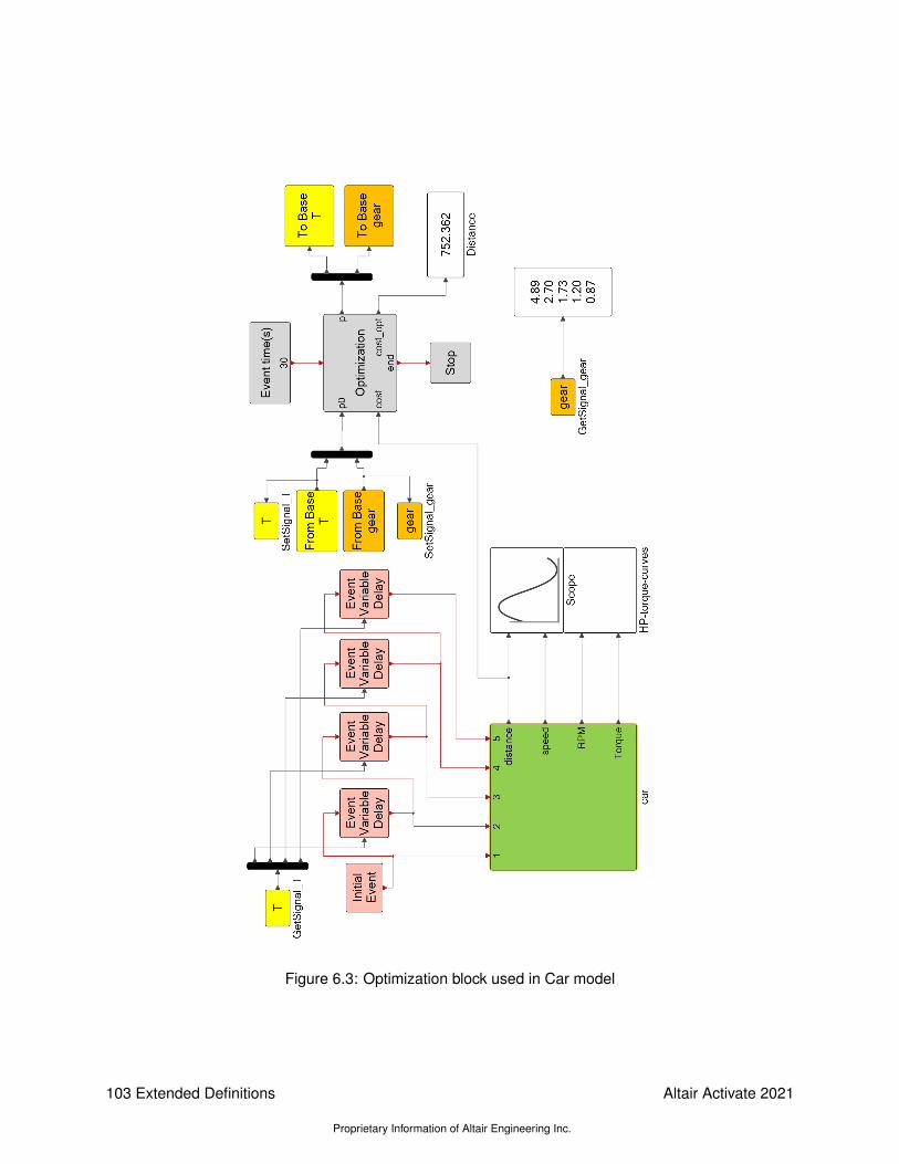
Figure 6.3: Optimization block used in Car model
103 Extended Definitions
Proprietary Information of Altair Engineering Inc.
Altair Activate 2021

Figure 6.4: BobyQA block dialog
Figure 6.5: Optimal path illustrated on the curve representing the engine power versus RPM
Altair Activate 2021
Proprietary Information of Altair Engineering Inc.
Extended Definitions 104

Figure 6.6: The RPM as a function time.
Figure 6.7: Distance and Speed results for the model car_max_dist_30sec.scm
105 Extended Definitions
Proprietary Information of Altair Engineering Inc.
Altair Activate 2021

The second optimization problem consists of minimizing the time to reach 1000m. In this case eachsimulation run is ended when the traveled distance goes beyond 1000m. The zero-crossing blockZeroCrossUp generates an event when this happens, activating the Optimization block, which readsthe cost value (in this case the time) and generates a new optimization vector p. Vector p is again theconcatenation of T and gear. The full model is shown in Fig. 6.8.
The optimization result shows that the vehicle reaches 1000m in 36.5 seconds. The optimal gear ratiosare different from the solution of the first problem.
In another problem formulation, reaching a given speed in the shortest possible time is considered.This problem is similar to the previous problem and the corresponding model is found in the filecar_min_time_speed_vtarget.scm and is illustrated in Fig. 6.9.
Note that an event at time 100 (final simulation time) is added to the event corresponding to reachingvtarget since depending on the gear ratios, the car may never reach the speed of vtarget. Thisproblem is considered again later to illustrate the use of an OML function to read data from the baseworkspace. Using this function, leads to simpler models as explained in the following section.
Optimal gear-change timing
It is interesting to note that the optimal gear chaning instants are the time instants where before andafter the gear change, the engine power has the same value, i.e., the transition is horizonal (see Fig.6.5). This of course is not a coincidence and can be shown to hold under very general assumptions,as it is shown below. The solution found by the optimizer having this property is an indication that theoptimization process has succeeded in finding the optimal solution.
To show that the optimal solution corresponds to a horizontal transition, consider the simpler problemwhere the car has only two gears, so the problem is to find the timing of the only possible gear change.The extension to the case of more than two gears is then straighforward.
The following image compares two gear shifting strategies corresponding to different gear changingtimes:
For both strategies (blue and red) the starting point is O. As time goes on, the RPM goes up with thepower following the black curve (representing the maximum engine horse power as a function of RPM).For the blue strategy the gear is shifted at point A transitioning the state of the system to point A′. Forthe red strategy, the gear shifting happens later, at point B, transitioning to B′. So both strategies follow
Altair Activate 2021
Proprietary Information of Altair Engineering Inc.
Extended Definitions 106
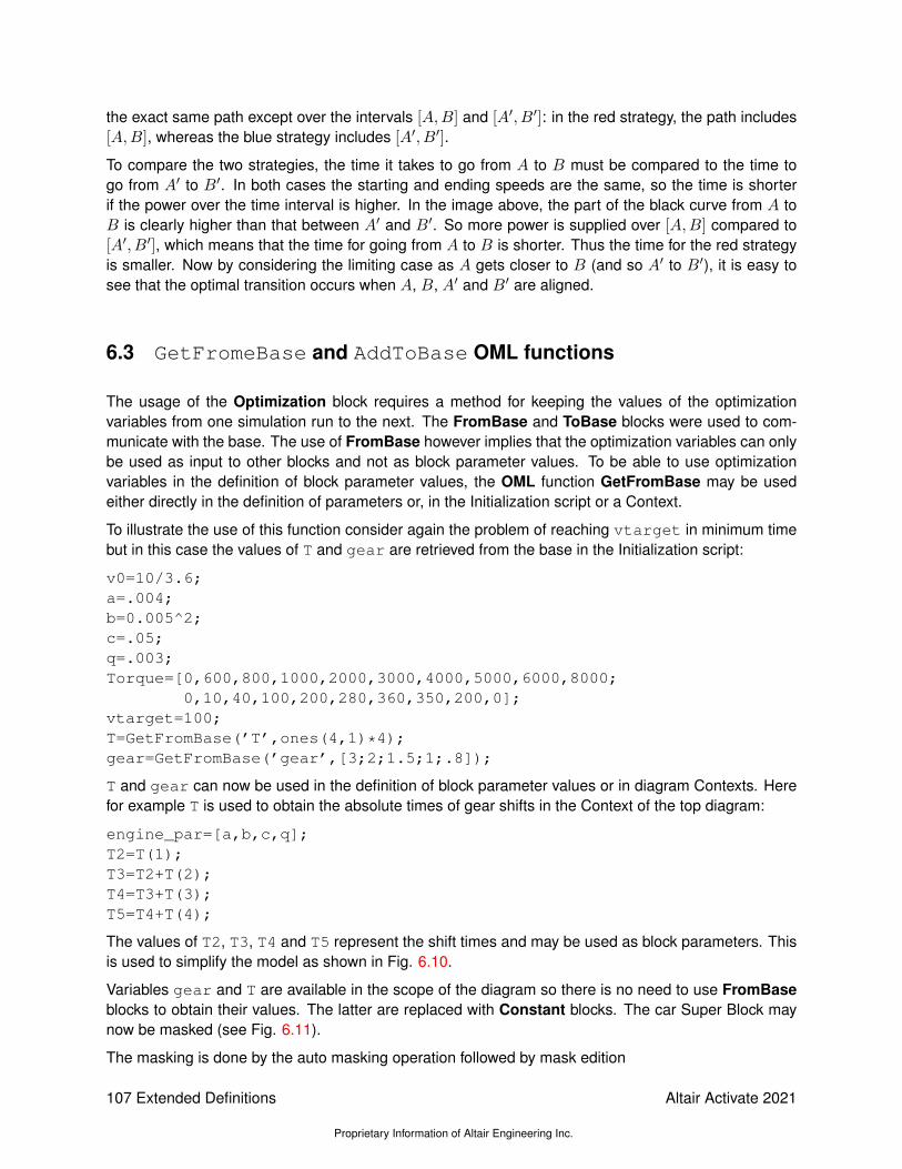
the exact same path except over the intervals [A,B] and [A′, B′]: in the red strategy, the path includes[A,B], whereas the blue strategy includes [A′, B′].
To compare the two strategies, the time it takes to go from A to B must be compared to the time togo from A′ to B′. In both cases the starting and ending speeds are the same, so the time is shorterif the power over the time interval is higher. In the image above, the part of the black curve from A toB is clearly higher than that between A′ and B′. So more power is supplied over [A,B] compared to[A′, B′], which means that the time for going from A to B is shorter. Thus the time for the red strategyis smaller. Now by considering the limiting case as A gets closer to B (and so A′ to B′), it is easy tosee that the optimal transition occurs when A, B, A′ and B′ are aligned.
6.3 GetFromeBase and AddToBase OML functions
The usage of the Optimization block requires a method for keeping the values of the optimizationvariables from one simulation run to the next. The FromBase and ToBase blocks were used to com-municate with the base. The use of FromBase however implies that the optimization variables can onlybe used as input to other blocks and not as block parameter values. To be able to use optimizationvariables in the definition of block parameter values, the OML function GetFromBase may be usedeither directly in the definition of parameters or, in the Initialization script or a Context.
To illustrate the use of this function consider again the problem of reaching vtarget in minimum timebut in this case the values of T and gear are retrieved from the base in the Initialization script:
v0=10/3.6;a=.004;b=0.005^2;c=.05;q=.003;Torque=[0,600,800,1000,2000,3000,4000,5000,6000,8000;
0,10,40,100,200,280,360,350,200,0];vtarget=100;T=GetFromBase(’T’,ones(4,1)*4);gear=GetFromBase(’gear’,[3;2;1.5;1;.8]);
T and gear can now be used in the definition of block parameter values or in diagram Contexts. Herefor example T is used to obtain the absolute times of gear shifts in the Context of the top diagram:
engine_par=[a,b,c,q];T2=T(1);T3=T2+T(2);T4=T3+T(3);T5=T4+T(4);
The values of T2, T3, T4 and T5 represent the shift times and may be used as block parameters. Thisis used to simplify the model as shown in Fig. 6.10.
Variables gear and T are available in the scope of the diagram so there is no need to use FromBaseblocks to obtain their values. The latter are replaced with Constant blocks. The car Super Block maynow be masked (see Fig. 6.11).
The masking is done by the auto masking operation followed by mask edition
107 Extended Definitions
Proprietary Information of Altair Engineering Inc.
Altair Activate 2021

Note that the optimization variables remain in the base after an optimization is run. So in order to restartan optimization process with the original initial values, the optimization variables must be removed fromthe base. This can be done using the clear function.
The OML function AddToBase may be used in the Initialization script or the Context to define orredefine a variable in the base.
Altair Activate 2021
Proprietary Information of Altair Engineering Inc.
Extended Definitions 108

Figure 6.8: Car model for minimizing time to distance (car_min_time_dist_1000m.scm)
109 Extended Definitions
Proprietary Information of Altair Engineering Inc.
Altair Activate 2021
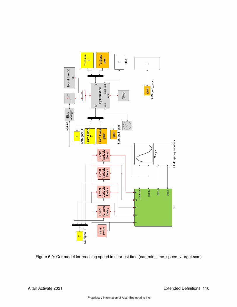
Figure 6.9: Car model for reaching speed in shortest time (car_min_time_speed_vtarget.scm)
Altair Activate 2021
Proprietary Information of Altair Engineering Inc.
Extended Definitions 110

Figure 6.10: Model variant (car_min_time_speed_vtarget_2.scm)
Figure 6.11: Masked "Car" superblock
111 Extended Definitions
Proprietary Information of Altair Engineering Inc.
Altair Activate 2021

6.4 Script based optimization
Script based optimization provides a powerful mechanism for solving very general optimization prob-lems where the cost and constraints may be obtained from a combination of Activate simulation resultsand an OML code. But in many cases, the cost is a simple function of signals generated by one ormore SignalOut blocks and the optimization problem formulation is straightforward yielding virtuallyalways the same OML script. For these simple cases, Activate provides a graphical tool for formulatingan optimization problem associated with a given model. This tool, which generates transparently therequired optimization script, is presented in Section 6.5. But first direct scripting is presented.
6.4.1 Direct scripting of optimization code in OML
The full power of OML may be used to solve optimization problems associated with Activate models.The code in OML would be the same as that for solving any optimization problem; the only specificity isthat the cost would depend entirely or partially on the result of a Activate simulation run. OML scriptsused for such optimizations may also be included inside the Activate model. See Chapter 20 for details.
Running a simulation from OML (in batch mode) requires creating a simulation object for the model.This object is needed to activate the graphical outputs of the Scopes present in the model. If graphicaloutputs are not needed, the simulation object is not needed.
The model evaluator is an OML function that is generated specifically for a given model. The evaluatorevaluates all model parameters and creates the flat model structure, which is used by the compiler tocreate the simulation structure. The model evaluator must be created before running the simulator butit can be created only once for a given model. As parameters are changed during simulation runs, theevaluator function is re-evaluated but the evaluator function itself does not need to be recreated.
Finally once the simulation object and the evaluator are created, the model may be simulated.
The OML functions corresponding to the above operations are:
• bdeCreateSimulationObject: This function creates a simulation object for a given modelspecified as an scm model file.
• vssCreateEvaluator: This function creates an evaluator for the given model.
• vssRunSimulation: This function is used to run a Activate simulation. The arguments in-clude the evaluation function of the model and various workspaces.
There are various ways to exchange data between OML and the Activate model. The most directway to change model parameters from OML is to use the vss_context workspace. Variables usedin a model for defining block parameters are defined in a workspace resulting from the execution ofthe Initialization script and various diagram Contexts following the semi-global scoping rule. When asimulation is run in batch mode, the workspace vss_context is injected in the workspace resultingfrom the execution of the Initialization script. Variables in vss_contextmay redefine variables definedin the Initialization script. In that case, the original values of the variables in the Initialization script canbe considered as default or initial values, which can be modified during batch simulation. Note also thatthe presence of these default/initial values are needed to make the model self-contained.
To get data back to OML from the simulation, the SignalOut block may be used. This block returns aSignal object in the working environment. This environment is passed to the batch simulation functionas optional argument.
Altair Activate 2021
Proprietary Information of Altair Engineering Inc.
Extended Definitions 112

6.4.2 Example
Consider again the optimization problem where the objective was to minimize the time to attain 1000mmark. The model is modified (Fig. 6.12) by removing the Optimization block and its supporting blocks.Variables T and gear are now defined in the Initialization script, and the simulation end time is returnedin Signal Tf.
Figure 6.12: Modified model for batch use with OML (car_min_time_distance_1000_batch.scm)
The Initialization script includes now the definition of T and gear:
This model can be simulated since all the required variables, in particular T and gear, are defined.For optimization purpose however the values of these variables must be overwritten. This will be doneusing the vss_context workspace as shown below.
The optimization script may use any of the existing OML optimization functions or coded directly inOML. The following script, car_min_time_distance_1000_batch.oml, uses the fminunconfunction.
113 Extended Definitions
Proprietary Information of Altair Engineering Inc.
Altair Activate 2021

function e=eval_cost(p,ev,env)vss_context=struct();vss_context.T=p(1:4);vss_context.gear=p(5:9);vssRunSimulation(ev,vss_context,env);Tf=getenvvalue(env,’Tf’);e=Tf.ch1.data;
end
me=omlfilename(’fullpath’);p=fileparts(me);model=[p,’/car_min_time_distance_1000_batch.scm’];T0=4*ones(4,1);gear0=[3.2;1.8;1.3;1;.8];p0=[T0;gear0];simobj=bdeCreateSimulationObject(model);ev=vssCreateEvaluator(model,simobj);env=getnewenv;cost=@(p) eval_cost(p,ev,env);options=optimset(’MaxFunEvals’,1000);p = fminunc(cost,p0,options);T=p([1:4])gear=p([5:9])
In the above example, the SignalOut block is used to return a single value (simulation time) but itcan be used to return the whole time trajectory of signals and be used to implement very complexoptimization scenarios.
In the following version of the gear ratio optimization problem, a constraint is imposed on the engineRPM. The problem is that of reaching a given speed as fast as possible without revving the engineabove a maximum RPM (for example 5500 RPM). The optimization methods used so far, BobyqaOptand fminuncon, did not allow the specification of such constraints. Bobyqa allowed bounds on theoptimization variables but in this case, the engine RPM is not directly an optimization variable. Tosolve such constrained problems, the OML function fmincon may be used. The function fmincon,in addition to a cost value, takes a vector of constraint values. This function minimizes the given costsubject to the constraint being below specified values.
To use fmincon, the Activate model must be extended to return the engine RPM. This is done insidethe signal omega as shown in Fig. 6.13
The optimization script is then as follows:
function e=ev_cost(p,ev,env)vss_context=struct();vss_context.T=p([1:4]);vss_context.gear=p([5:9]);vssRunSimulation(ev,vss_context,env);Tf=getenvvalue(env,’Tf’);e = Tf.ch1.data;if isempty(e) e=100; end
end
Altair Activate 2021
Proprietary Information of Altair Engineering Inc.
Extended Definitions 114

Figure 6.13: Model extended to return the omega signal(car_min_time_speed_vtarget_w_constr_batch.scm)
function c=ev_constr(p,ev,env)vss_context=struct();vss_context.T=p([1:4]);vss_context.gear=p([5:9]);vssRunSimulation(ev,vss_context,env);omega=getenvvalue(env,’omega’);w = omega.ch1.data;c=max(w)-5500;
end
me=omlfilename(’fullpath’);p=fileparts(me);
115 Extended Definitions
Proprietary Information of Altair Engineering Inc.
Altair Activate 2021

model=[p,’/car_min_time_speed_vtarget_w_constr_batch.scm’];
T0=5*ones(4,1);gear0=[3.2;1.8;1.3;1;.8];p0=[T0;gear0];lb=.1*ones(9,1);ub=20*ones(9,1);simobj=bdeCreateSimulationObject(model);ev=vssCreateEvaluator(model,simobj);env=getnewenv;cost=@(p) ev_cost(p,ev,env);constr=@(p) ev_constr(p,ev,env);options=optimset(’MaxFunEvals’,1000);p = fmincon(cost,p0,[],[],[],[],lb,ub,constr,options);T=p([1:4])gear=p([5:9])
After execution of the optimization script, the optimal time evolution of the RPM is obtained as shown inFig. 6.14.
Figure 6.14: RPM vs. time after optimization.
The vehicle reaches 100Km/h in 15.9 seconds. Without the 5500 RPM constraint, the time was15.76sec.
In this example, the constraint value, i.e., the maximum over the RPM signal was computed inside theOML function ev_constr. For that, the complete signal time history, omega, was returned to OML.The maximum value could have also been computed in the model and simply its final value returned toOML but that would have required adding a few more blocks to the diagram. In general the computationof the cost function and constraint values could be done partly in the model, partly in the OML code.
Altair Activate 2021
Proprietary Information of Altair Engineering Inc.
Extended Definitions 116

Figure 6.15: Horse power as a function of RPM after optimization.
6.5 Activate Graphical optimization tool
The graphical interactive optimization tool generates and runs automatically the OML scripts for solvingActivate optimization problems. The tool can be used to associate optimization criteria to an existingActivate model. In particular it provides a simple to use interface for defining optimization variables anddefining cost and constraints.
The tool should be seen as a graphical interface for the OML optimization functions fminuncon,fmincon and ga. The interface is associated with a Activate model, or more specifically with an scmfile (the distinction is important since the modifications to the model are not taken into account until themodel is saved). The information that needs to be provided in the interface is as follows:
• Model path: The association is done by entering the path of the scm file containing the Activatemodel.
• Initialization: An OML code must be provided. Any variable defined in this code overwrites vari-ables defined in the Initialization script of the model. The initial (guess) values of the optimizationvariables should not be defined in this code; they will be defined later. Variables needed to definethem however may be defined here.
• Number of variables: The number of optimization variables must be given here. Depending onthis number, the user is presented with a list of widgets were he should provide the name, theinitial value and the range (min and max values) of each variable. The initial value may be definedas an expression using variables defined in the Initialization code. If the variable is a vector ormatrix, the min and max values may be given as scalars, otherwise their sizes should match thatof the variable.
• Number of constraints: The number of inequality constraints must be specified. This number,which may be defined as an expression using variables defined in the Initialization code, must
117 Extended Definitions
Proprietary Information of Altair Engineering Inc.
Altair Activate 2021

match the size of the _constraint vector defined in the Optimization script when the optimiza-tion problem contains constraints.
• Optimization script: An OML code used to define the variable _cost and, if the problem hasconstraints, the vector _constraint. The code may assume that all the variables defined inthe Initialization code, all the signals associated with SignalOut blocks present in the model, inaddition to the current values of the optimization variables produced by the optimizer are in itsworkspace. The optimizer searches the optimization variables within the specified bounds suchthat all the elements of _constraint are negative and the _cost is minimal.
• Optimization method: SQP and Genetic algorithm are proposed. More methods will be includedin the future. SQP uses the OML functions fmincon or fminbnd functions depending on thepresence or absence of constraints. The genetic algorithm uses ga.
• Depending on the selected optimization method, different optimization parameters such as Maxnumber of iterations, Convergence tolerance, Constraint tolerance, Population size, etc., must beprovided. These parameters are passed to the underlying OML optimization routine. See OMLdocumentation for details.
The graphical interface provides, at the end of the simulation, the optimal cost, the number of iterationsand gives access to the generated OML script. The cost value history versus the iteration number mayalso be plotted.
The solution to the problem is returned in the base environment inside the OML table _optim. Inaddition to the optimal values of the optimization variables, the table includes the optimal cost and theirhistories for all the iterations performed during optimization.
The optimization may be started using the run button on top of the graphical interface once all therequired information is provided. At every step, the proposed values for the optimization parametersand the associated costs are displayed. The optimization process may be stopped at any time usingthe stop button.
The use of the tool is quite intuitive and is illustrated here through an example.
6.5.1 Example
The constrained optimization problem considered previously and solved using OML scripting is consid-ered again, and formulated and solved with the graphical optimization tool. The problem is to find thebest gear ratios to reach a given speed as fast as possible with constraint on the top RPM. The sameActivate model is used. The top RPM will be parameterized without modifying the model.
The graphical optimization tool corresponding to this problem may be created as shown in Fig. 6.16and run using the Run button on top.
The Initialization code used in the optimization tool is virtually identical to the model Initialization script(see Fig. 6.17).
But instead of T and gear, it defines their initial values. Note that all model parameters may be modifieddirectly in the tool without requiring any modifications of the Activate model. So the end user does noteven have to see the simulation model to run optimizations for different sets of parameters. For exampleoptimization may be performed for different values of target speed and top RPM. All vehicle parameters,including the Torque curve can also be modified.
Altair Activate 2021
Proprietary Information of Altair Engineering Inc.
Extended Definitions 118

Figure 6.16: Optimization Tool
Figure 6.17: Initialization script used in the Optimization Tool
The bounds on the optimization variables T and gear are set as scalars. The time increment is alwayspositive, so is the gear ratio which is assumed to be arbitrarily greater than 0.1 (0 value would bemeaningless).
The number of constraints is set to 1 and the variables _cost and _constraint are defined asfollows (Fig. 6.18):
Note the use of the signals Tf and omega produced by the SignalOut blocks of the model. The Tfsignal however may be empty since the vehicle does not always reach the target speed before the endof the simulation. If that happens the cost is set to infinity so that the optimization may proceed. Theoptimization variables could also be used in defining the cost and constraints. Note however that theywould have their current values as decided by the optimizer at the current step of the optimization andnot necessarily their original values defined in the Initialization code.
Running the simulation gives the same result obtained previously with direct scripting. The optimal
119 Extended Definitions
Proprietary Information of Altair Engineering Inc.
Altair Activate 2021

Figure 6.18: Constraint definition in the Optimization Tool
values of T and gear, and the optimal cost in addition to other information are available in Table_optim subsequent to running the optimization.
6.6 Max-min/Min-max optimization problems
Max-min and Min-max optimization problems may be formulated in different ways in Activate. Forexample the min part may be implemented using the Optimization block and the max in OML. Thefollowing example illustrates such an implementation. In this example, the robust version of the gearshifting problem is considered. It is assumed that gear shifting does not occur at prescribed times butthey could happen up to a timing error of 0.1 seconds before or after the specified times. The opti-mization problem consists in optimizing the performance corresponding to the worst case time errors.In particular, the Activate model is modified such that the traveled distance is minimized over possiblevalues dT of the timing error vector. It is then this value which is used as cost to maximize.
The Max-min problem is formulated in the model shown in Fig. 6.19) and is then realized using theOML optimization script generated by the Optimization tool (see Fig. 6.20).
Max-min and Min-max optimization problems may also be formulated by using multiple Optimizationblocks. In general only one such block may be used in a model but more than one block may be usedif they are cascaded as illustrated in the diagram of Fig. 6.21 which implements the same Max-minproblem considered previously.
Altair Activate 2021
Proprietary Information of Altair Engineering Inc.
Extended Definitions 120
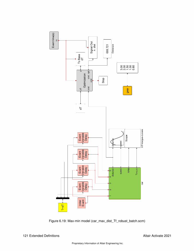
Figure 6.19: Max-min model (car_max_dist_Tf_robust_batch.scm)
121 Extended Definitions
Proprietary Information of Altair Engineering Inc.
Altair Activate 2021

Figure 6.20: Optimization tool for the Max-Min problem for Model in figure 6.19.
Altair Activate 2021
Proprietary Information of Altair Engineering Inc.
Extended Definitions 122

Figure 6.21: Variant of the Max-min model (car_max_dist_Tf_robust.scm)
123 Extended Definitions
Proprietary Information of Altair Engineering Inc.
Altair Activate 2021

Figure 6.22: RPM as a function of time after optimization in Model in Fig. 6.21.
Altair Activate 2021
Proprietary Information of Altair Engineering Inc.
Extended Definitions 124

Chapter 7
Linearization
7.1 Linearization function
Activate provides functions to create linear models from a Super Block by linearization. Lineariza-tion consists of constructing an approximate linear model around a given equilibrium (operating) point.Linearized models are constructed in particular for analysis and, controller and filter design.
The equilibrium point for the system
x = f(x, u)
y = h(x, u)
is defined as the triplet (xe, ue, ye) satisfying
0 = f(xe, ue)
ye = h(xe, ue).
The linearization of this system around the equilibrium point (xe, ue, ye) is a linear state-space systemspecified in terms of 4 matrices A, B, C and D:
˙δx = Aδx+Bδu
δy = Cδx+Dδu
where δx = x− xe, δu = u− ue, δy = y − ye, and
A =∂f
∂x(xe, ue), B =
∂f
∂u(xe, ue), C =
∂h
∂x(xe, ue), D =
∂h
∂u(xe, ue).
The main function to perform linearization in OML is vssLinearizeSuperBlock: and is used asfollows
[A,B,C,D] = vssLinearizeSuperBlock(model,sblk,inps,outs,tf,ctx);
The first argument, model, representing the model in which linearization is to be performed, can eitherbe a path of an scm file or a model object. The latter in general is the current model which can beobtained by the bdeGetCurrentModel function.
125 Extended Definitions
Proprietary Information of Altair Engineering Inc.
Altair Activate 2021

The second argument is the full name of the Super Block being linearized. The linearization is notnecessarily performed with respect to all the inputs and outputs. Some of the inputs, in general corre-sponding to discrete-time signals, may have to be excluded. Similarly some outputs may need to beexcluded. The arguments inps and outs are vectors of indices representing respectively the inputsand outputs to be considered for linearization.
The time tf is the time up to which the simulation is performed (in general to reach an equilibrium point)before linearization is done. The value of tf can be set to zero if the model is already in an equilibriumpoint (possibly thanks to the following argument ctx described below).
The final argument, ctx, is an external context, used to overwrite some of the variables defined in theInitialization script of the model. This is done in general to put the model in an equilibrium point withoutmodifying it.
The function returns the (A,B,C,D) matrices of the linearized model.
7.1.1 Example: inverted pendulum
The classical problem of controlling an inverted pendulum mounted on a cart is considered. The ob-jective is to control the force applied to the cart in such a way that the pendulum is stabilized pointingupwards. The force moves the cart on a ramp.
Figure 7.1: Inverted Pendulum on a ramp
Two sensors provide the position of the cart and the angle of the pendulum to the controller.
The equations of motion of the system may be expressed as follows:(M +m)z +mlθ cos(θ − φ)/2−mlθ2 sin(θ − φ)/2 = u(t)− (M +m)g sin(φ)
(J +ml2/4)θ +mlz cos(θ − φ)/2−mgl sin(θ)/2 = 0
M represents the mass of the cart, and m the mass of the pendulum. The moment of inertia of thependulum, considered to be a homogeneous bar, is J = ml2/12. The cart moves on a rail placed on aramp with an angle φ.
The system variables z and θ represent respectively the position of the cart on the ramp and the angleof the pendulum. The angle zero corresponds to the vertical position, pointing up.
Altair Activate 2021
Proprietary Information of Altair Engineering Inc.
Extended Definitions 126

The system may be re-expressed in matrix form as follows:(M +m ml cos(θ − φ)/2
ml cos(θ − φ)/2 J +ml2/4
)(z
θ
)=
(mlz2 sin(θ − φ)/2 + u− (M +m)g sin(φ)
mgl sin(θ)
)
The matrix on the left is square and invertible (provided m > 0), so z and θ may be computed byusing a simple matrix formula. So the cart pendulum system may be implemented in Activate usingthe MatrixExpression block as shown in Fig. 7.2.
Figure 7.2: Pendulum superblock inside Inverted Pendulum model (inv_pendulum0.scm).
The parameters of the system are defined in the Super Block Context as follows:
m=1;M=4;l=.7;g=9.8;J=m*l^2/12;
The complete model is illustrated in Fig. 7.3. Note that the controller is a state space linear system withparameters At, Bt, Ct.
Figure 7.3: Inverted Pendulum model (inv_pendulum0.scm).
127 Extended Definitions
Proprietary Information of Altair Engineering Inc.
Altair Activate 2021

The model is designed in such a way that the simulation can be preformed both with and without alinearized model. In the absence of a linearized model, a “zero” controller (controller producing zero asoutput) is used. This is done in the Context of the top diagram as follows:
_syslin=GetFromBase(’_syslin’,[]);if isempty(_syslin)
At=[];Bt=zeros(0,2);Ct=zeros(1,0);
elseA=_syslin.a;B=_syslin.b;C=_syslin.c;D=_syslin.d;n=size(A,1);Kc=-place(A,B,-1*ones(1,n));Kf=-place(A’,C’,-2*ones(1,n));Kf=Kf’;
At=A+B*Kc+Kf*C+Kf*D*Kc;Bt=-Kf;Ct=Kc;
end
So if a structure called _syslin is defined in the base environment, it is used as the linearized modelto design an observer-based controller. If not, the controller is set to zero. This way, when the model islinearized, the linearization is performed in the “open-loop” case (i.e., the plant alone).
The linearization can be performed with the following script:
clear(’_syslin’);% vector of input port indices considered for linearizationinps = 1;% vector of output port indices considered for linearizationouts = [1,2];% Modified contextctx=struct;ctx.z0 = 0;ctx.th0 = 0;ctx.phi = 0;
model=bdeGetCurrentModel;% Selected Super block to linearizesuperblock = ’pendulum’;
[A,B,C,D]=vssLinearizeSuperBlock(model,superblock,inps,outs,0,ctx);_syslin.a=A;_syslin.b=B;_syslin.c=C;_syslin.d=D;
Altair Activate 2021
Proprietary Information of Altair Engineering Inc.
Extended Definitions 128
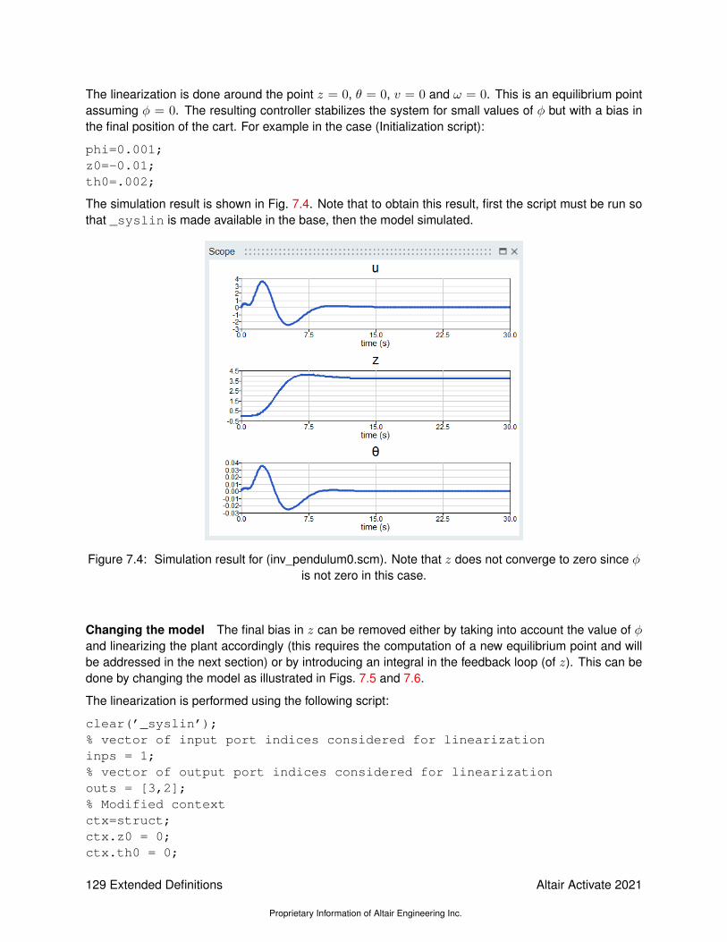
The linearization is done around the point z = 0, θ = 0, v = 0 and ω = 0. This is an equilibrium pointassuming φ = 0. The resulting controller stabilizes the system for small values of φ but with a bias inthe final position of the cart. For example in the case (Initialization script):
phi=0.001;z0=-0.01;th0=.002;
The simulation result is shown in Fig. 7.4. Note that to obtain this result, first the script must be run sothat _syslin is made available in the base, then the model simulated.
Figure 7.4: Simulation result for (inv_pendulum0.scm). Note that z does not converge to zero since φis not zero in this case.
Changing the model The final bias in z can be removed either by taking into account the value of φand linearizing the plant accordingly (this requires the computation of a new equilibrium point and willbe addressed in the next section) or by introducing an integral in the feedback loop (of z). This can bedone by changing the model as illustrated in Figs. 7.5 and 7.6.
The linearization is performed using the following script:
clear(’_syslin’);% vector of input port indices considered for linearizationinps = 1;% vector of output port indices considered for linearizationouts = [3,2];% Modified contextctx=struct;ctx.z0 = 0;ctx.th0 = 0;
129 Extended Definitions
Proprietary Information of Altair Engineering Inc.
Altair Activate 2021

Figure 7.5: Pendulum_integral superblock inside the Inverted Pendulum model(inv_pendulum_integral.scm). The integral of z is added as an output to be used for feedback control.
Figure 7.6: Inverted Pendulum model (inv_pendulum_integral.scm).
ctx.phi = 0;
model=bdeGetCurrentModel;% Selected Super block to linearizesuperblock = ’pendulum_integral’;
% Linearization[A,B,C,D]=vssLinearizeSuperBlock(model,superblock,inps,outs,0,ctx);_syslin.a=A;_syslin.b=B;_syslin.c=C;_syslin.d=D;
Note that only the second and third outputs of the Super Block (in the reverse order) are used in thedefinition of the Plant to be linearized. The simulation result is shown in Fig. 7.7. The bias is removedthanks to the integral in the loop.
To simplify the use of the function vssLinearizeSuperBlock for a given Super Block, the menuLinearize is provided. By selecting a Super Block and using the contextual menu Linearize, an
Altair Activate 2021
Proprietary Information of Altair Engineering Inc.
Extended Definitions 130
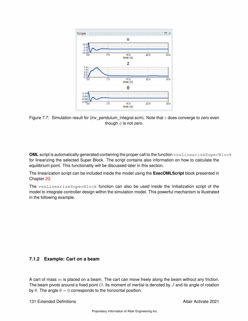
Figure 7.7: Simulation result for (inv_pendulum_integral.scm). Note that z does converge to zero eventhough φ is not zero.
OML script is automatically generated containing the proper call to the function vssLinearizeSuperBlockfor linearizing the selected Super Block. The script contains also information on how to calculate theequilibrium point. This functionality will be discussed later in this section.
The linearization script can be included inside the model using the ExecOMLScript block presented inChapter 20.
The vssLinearizeSuperBlock function can also be used inside the Initialization script of themodel to integrate controller design within the simulation model. This powerful mechanism is illustratedin the following example.
7.1.2 Example: Cart on a beam
A cart of mass m is placed on a beam. The cart can move freely along the beam without any friction.The beam pivots around a fixed point O. Its moment of inertial is denoted by J and its angle of rotationby θ. The angle θ = 0 corresponds to the horizontal position.
131 Extended Definitions
Proprietary Information of Altair Engineering Inc.
Altair Activate 2021

The variable z denotes the projection of the center of mass of the cart on the beam; the zero positioncorresponds to the point O. The height of the center of mass of the cart (its distance to the beam) isdenoted h.
The mechanism is controlled by applying a torque T to the beam around the point O. The objective ofthe control is to stabilize the cart on the beam.
The equations of motion for this system can be expressed as follows:
mz = mzθ2 −mg sin(θ)
(J +mz2)θ = T − 2mzzθ −mgz cos(θ) +mgh sin(θ)
The objective is to design an observer-based controller for the system. This is done by first lineariz-ing the system, then designing an observer-based controller for the linearized model. The measuredoutputs are considered to be the angle θ and the position z:
y =
(zθ
).
The control input is u = T . So the system has four states, one input and two outputs.
The system is modeled in Modelica language as follows
model cart//parametersparameter Real h = 1;parameter Real m = 2;parameter Real J = 10;parameter Real th0 = 0;parameter Real z0 = 0;//input variablesReal T;//output variablesReal z(start=z0), th(start=th0);Real zd(start=0), thd(start=0);Real g=9.81;
Altair Activate 2021
Proprietary Information of Altair Engineering Inc.
Extended Definitions 132

equationder(th)=thd;der(z)=zd;der(zd) = z*thd*thd-m*g*sin(th);(J+m*z*z)*der(thd) = T-2*m*z*zd*thd-
m*g*z*cos(th)+m*g*h*sin(th);end cart;
which is implemented using a Custom Modelica block. The system could also be implemented usingstandard Activate blocks.
The Activate model is given in Fig. 7.8 and 7.9.
Figure 7.8: The model of the cart on beam system with an observer-based controller.
Figure 7.9: Inside the ’cart on beam’ Super Block being linearized.
Figure 7.10: The parameters tab of the Custom Modelica block dialog GUI.
The initial position of the cart and the initial angle of the beam, z0 and th0, are not necessarily zero forsimulation but must be set to zero for linearization. This is done in the Initialization script of the model
133 Extended Definitions
Proprietary Information of Altair Engineering Inc.
Altair Activate 2021

as follows:
h=1; m=2; J=10;nx=4;nu=1;ny=2;th0=pi/12;z0=-1;
if ~vssIsInLinearizationctx=struct;ctx.K=zeros(1,nx);ctx.obs=ss([],zeros(0,nu+ny),zeros(nx,0),zeros(nx,nu+ny));ctx.th0=0;ctx.z0=0;[A,B,C,D]=vssLinearizeSuperBlock(bdeGetCurrentModel,...’cart on beam’,[1],[1],0,ctx);L=-place(A’,C’,-3*ones(nx,1))’;obs=ss(A+L*C,[B+L*D,-L],eye(nx),zeros(nx,nu+ny));K=-place(A,B,-3*ones(nx,1));
end
The variable vssIsInLinearization is false in general; it is true only when the Initialization scriptis executed in the phase of linearization (the model is evaluated and simulated for linearization). As itcan be seen in the script, when the model is in the linearization stage, the controller gain K is set tozero and the observer obs similarly to a trivial linear system. This is done through the external contextctx. ctx is used also to set to zero the initial states for linearization.
When the script is not used in the linearization stage, the observer-based controller is constructedand used for simulation. To construct an observer-based controller for a linear system (A,B,C,D),a feedback gain matrix K is found such that A + BK is Hurwitz (all eignvalues have strictly negativereal parts) and an observer gain L is found such that A + LC is Hurwitz. This is possible as long asthe system is stabilizable and detectable. Here the pole placement OML function place is used tocompute K and L.
So when this model is simulated, the Super Block’cart on beam’ is linearized, the result of linearizationis used to construct the observer-based controller, and the simulation of the resulting model for nonzero initial conditions is performed. The simulation result is shown in Fig. 7.11.
Changing the system The model used above uses the model of a cart on a beam with the controlbeing the torque applied to the beam. The model however, and in particular the Initialization script doesnot use any information related to the underlying system defined inside the Super Block that it controlsexcept input, output and state sizes and certain system parameters. So this construction is very genericand can be applied to any other system placed inside the Super Block by bringing small adjustments tothe Initialization script.
Consider here the following modification of this example: instead of the control being a torque applied tothe beam, it is now a force applied to the cart at the level of its wheels (along the beam). The equationsof motion the become:
mz = mzθ2 −mg sin(θ) + T
(J +mz2)θ = −2mzzθ −mgz cos(θ) +mgh sin(θ)
Altair Activate 2021
Proprietary Information of Altair Engineering Inc.
Extended Definitions 134

Figure 7.11: The simulation result shows that the system is stabilized.
where T represents now the applied force. This new system can now be placed inside the SuperBlock and no other modification is required. This is done in Model cart_on_beam_force.scm. Thesimulation shows that the controller is properly constructed and the system is stabilized.
Stabilizing the cart off center Consider now the problem of stabilizing the cart not at the center ofthe beam but at a different location. A possible approach would be to use the exact same model butintroduce a bias in the output of the system before feeding it to the controller, y0. See Fig. 7.12. Theidea being that the controller will drive y-y0 to zero thus imposing the desired output.
The variable y0 is defined in the Initialization script as follows
zobj=0.2;y0=[zobj;0];
The value of zobj corresponds to the location where the cart is to be stabilized. The simulation resultis shown in Fig. 7.13. It can be seen that even though the use of bias has moved the location of thecart, the desired value zobj is not achieved. The reason is that the steady-state gain of the controlleris not infinite.
Figure 7.12: The model of the ’cart on beam’ system with an observer-based controller.
135 Extended Definitions
Proprietary Information of Altair Engineering Inc.
Altair Activate 2021

Figure 7.13: The simulation result shows that the cart is stabilized off the center of the beam but not atthe desired location.
An alternative solution for stabilizing the cart off center is to linearize the system off center. For that, anequilibrium point must be found. The solution which consists of running the simulation for certain timecannot be used in this case because the system is unstable in open loop. The equilibrium point shouldthen be computed differently.
7.2 Computation of the equilibrium point
The function vssEquilibriumPointSuperBlock is provided for finding equilibrium points by mod-ifying model parameters defined by the user. The simple usage of this function is as follows
[ctx,err]=vssEquilibriumPointSuperBlock(model,sblk,ctx,params);
The first three input arguments of the function are identical to that of vssLinearizeSuperBlockfunction seen above. The cell array params contains the list of variable names in the ctx that canbe modified by the function in order to set the state derivatives of all the continuous-time states of theblocks inside the Super Block sblk to zero. ctx is returned with the value of these variables modified.
In the cart on the beam example, the equilibrium state is known x0=[zobj;0;0;0], so is the equi-librium output y0=[zobj;0], which is imposed. What is unknown is the equilibrium input u0.
The Activate model using this function is given in Fig. 7.14 This is done in the Initialization script of themodel as follows:
h=1; m=2; J=10;nx=4;nu=1;ny=2;th0=pi/50;z0=0.5;zobj=1;y0=[zobj;0];
Altair Activate 2021
Proprietary Information of Altair Engineering Inc.
Extended Definitions 136

Figure 7.14: The model of the cart on beam stabilized with a controller linearized off center.
if ~vssIsInLinearizationctx=struct;ctx.K=zeros(1,nx);ctx.obs=ss([],zeros(0,nu+ny),zeros(nx,0),zeros(nx,nu+ny));ctx.th0=0;ctx.z0=zobj;ctx.u0=0;model=bdeGetCurrentModel;ctx=vssEquilibriumPointSuperBlock(model,...
’cart on beam’,ctx,’u0’);[A,B,C,D]=vssLinearizeSuperBlock(model,...’cart on beam’,[1],[1],0,ctx);L=-place(A’,C’,-7*ones(nx,1))’;obs=ss(A+L*C,[B+L*D,-L],eye(nx),zeros(nx,nu+ny));K=-place(A,B,-7*ones(nx,1));u0=ctx.u0;
end
The simulation results shows that the desired location is achieved. See Fig. 7.15
The vssEquilibriumPointSuperBlock function has additional optional arguments:
[ctx,err]=vssEquilibriumPointSuperBlock(model,sblk,ctx,params,inps,outs,L,M,verb);
The optional argument inps is used to set the time-dependency of the inputs of the superblock toconsider for the computation of the equilibrium point. This time dependency can also be set directlyinside the diagram by checking the time-dependency parameter of the corresponding input port blocks.The input sizes can also be defined by setting the parameters of these blocks. This may be requiredsince in some cases the compiler may not be able to determine port sizes by considering only thediagram inside of the Super Block. inps is a vector containing port numbers and its default value is[].
The optional argument outs specifies the outputs of the Super Block to take into account in the con-struction of the output vector y. The default is [].
The L and Mmatrices specify the vector which is set to zero by vssEquilibriumPointSuperBlock.This vector is: [L*xdot;M*y]. The default values are 1. If L is set to [], L*xdot is excluded fromthe vector. Similarly, If M is set to [], M*y is excluded from the vector.
If the optional argument verb is set to the string ’v’, the verbose mode is turned on. In this mode,
137 Extended Definitions
Proprietary Information of Altair Engineering Inc.
Altair Activate 2021

Figure 7.15: The simulation result shows that the objective is achieved.
the values tried by the solver and the corresponding vector [L*xdot;M*y] are displayed at eachiteration. This mode is useful for debugging.
So in general the vssEquilibriumPointSuperBlock function can be used to use the specifiedparameters to set parts or all of the state derivatives xdot and the outputs y to zero. A systematicapproach to finding the equilibrium point of a system is to construct the corresponding Super Block sothat the inputs and output are respectively δu = u − ue and δy = y − ye. These modifications canbe introduced using Bias blocks. The bias values ue and ye may be partially imposed, partially free forfinding the equilibrium point.
Consider again the cart on the beam example. To obtain the equilibrium point previously, the value ofthe equilibrium state xe was “guessed” from the value of the ye, and the only free variable was ue. Inparticular it was noted that the values of ze and θe are equal to the values specified in ye.
Here, instead of guessing the values of ze and θe, a systematic approach is used. This is done bycreating the Super Block by including bias terms so that the input and output are δu = u − ue andδy = y − ye. See Fig. 7.16.
7.2.1 Use of infinite steady-state gain controller
It was seen that simply by introducing a bias on the output of the controller designed for stabilizingthe cart at the center stabilizes the cart off center. However the location of the stabilization does notcorrespond to the desired location because of the finite steady-state controller gain. If a controller withinfinite gain is used, stabilization at the desired location can be achieved.
A way to obtain infinite steady-state gain is to introduce explicitly an integrator in the system. This isdone in the model shown in Fig. 7.17 and 7.18.
The Initialization script in this case is
Altair Activate 2021
Proprietary Information of Altair Engineering Inc.
Extended Definitions 138

Figure 7.16: The Plant Super Block is used for computing the equilibirum point and linearization. Seedemo model cart_on_beam_off_center_ep.scm.
Figure 7.17: The model of the cart using an infinite steady-state gain controller.
h=1; m=2; J=10;nx=5;nu=1;ny=2;th0=pi/50;z0=0.01;zobj=0.025;y0=[zobj;0];
if ~vssIsInLinearizationctx=struct;ctx.K=zeros(1,nx);ctx.obs=ss([],zeros(0,nu+ny),zeros(nx,0),zeros(nx,nu+ny));ctx.th0=0;ctx.z0=0;ctx.zobj=0;model=bdeGetCurrentModel;[A,B,C,D]=vssLinearizeSuperBlock(model,...’cart on beam’,[1],[2],0,ctx);L=-place(A’,C’,-5*ones(nx,1))’;obs=ss(A+L*C,[B+L*D,-L],eye(nx),zeros(nx,nu+ny));K=-place(A,B,-5*ones(nx,1));
end
Note that for the linearization only the second output is taken into account. This is the output which isconnected to the controller. The first output corresponding to the actual outputs of the system is usedfor display only.
The simulation result is shown in Fig. 7.19.
139 Extended Definitions
Proprietary Information of Altair Engineering Inc.
Altair Activate 2021

Figure 7.18: Inside the cart on beam Super Block. An integrator is included to force infinitesteady-state gain.
The advantage of using this approach is that the value of zobj is not used in the design process andit can be changed during the simulation. The model in Fig. 7.20 is similar to the previous model exceptthat instead of the desired location being defined by a constant zobj, it is a time varying signal (asquare wave in particular).
For the linearization in this case the first input and the second output are taken into account.The simu-lation result is shown in Fig. 7.22.
7.2.2 Equilibrium point for the inverted pendulum example
Consider again the inverted pendulum problem considered in the previous section. Here the assump-tion is made that the value of φ is known so the Plant can be linearized around the equilibrium pointcorresponding to the given value of φ. In this case the input is not linearized around 0 but a value U,which must be determined so that the system is in an equilibrium point. The equilibrium state here iszero.
The input bias U is introduced as shown in Fig.7.23. The value of U is not known and must be deter-mined by the computation of the equilibrium point.
The computation of the equilibrium point and linearization is performed with the following script:
clear(’_syslin’);% vector of input port indices considered for linearizationinps = 1;% vector of output port indices considered for linearizationouts = 1:2;% Modified contextctx=struct;ctx.z0 = 0;ctx.th0 = 0;ctx.U = 0;
model=bdeGetCurrentModel;
Altair Activate 2021
Proprietary Information of Altair Engineering Inc.
Extended Definitions 140

Figure 7.19: The simulation result shows that the system is stabilized at the desired location.
Figure 7.20: The inside of the ’cart on beam’ Super Block is shown in Fig. 7.21.
% Selected Super block to linearizesuperblock = ’pendulum’;% variables in ctx allowed to adjustvars=’U’;ctx=vssEquilibriumPointSuperBlock(model,superblock,ctx,vars,inps,outs,1,[],’v’);% Linearization[A,B,C,D]=vssLinearizeSuperBlock(model,superblock,inps,outs,0,ctx);_syslin.a=A;_syslin.b=B;_syslin.c=C;_syslin.d=D;_syslin.u0=ctx.U;
The verbose mode is used to monitor the progress of the optimization code computing the equilibriumpoint.
141 Extended Definitions
Proprietary Information of Altair Engineering Inc.
Altair Activate 2021

Figure 7.21: Inside the cart on beam Super Block. An integrator is included to force infinitesteady-state gain.
The resulting simulation result is shown in Fig.7.24.
Altair Activate 2021
Proprietary Information of Altair Engineering Inc.
Extended Definitions 142

Figure 7.22: The simulation result shows that the location of the cart follows the square wavereference trajectory.
Figure 7.23: Inverted Pendulum model (inv_pendulum.scm).
143 Extended Definitions
Proprietary Information of Altair Engineering Inc.
Altair Activate 2021

Figure 7.24: Simulation result for (inv_pendulum.scm). Note that z converges to zero.
Altair Activate 2021
Proprietary Information of Altair Engineering Inc.
Extended Definitions 144

7.2.3 3D model of a spacecraft for take off and landing control
The model of the spacecraft is made of two bodies connected by a universal joint. The distance fromthe joint to the center of mass of the top body, (x0, y0, z0), is denoted l0, and the distance to the bottombody’s center of mass, (x1, y2, z3), is dentoed l1. The top body is the main body of the spacecraft. Ithas mass m0 with moments of inertia along the main axes I0z and I0x = I0y. The propulsion system islodged in the second body, which has mass m1 and inertia I1z and I1x = I1y.
The coordinate system used to describe the dynamics of the system is attached to the universal joint.Its center is denoted (x,y, z), the joint axis connected to the bottom body is the x axis of the systemand the joint axis connected to the top body is the y axis of the system. The angle between the z axisand the main axis of the top body is denoted α and with the bottom body, β. The two bodies are alignedwhen α and β are zero.
The spacecraft is controlled via the propulsion force F applied orthogonal to the bottom body, at itscenter, and two torques to modify the angles α and β at the universal joint. The torques can beproduced by motors mounted on the bodies and acting (for example through a belt system) on theuniversal joint.
Euler angles The orientation of the coordinate system attached to the universal joint can be ex-pressed by Euler angles. There are various ways to define Euler angles corresponding to the axischoices and orders in which rotations are applied. The commonly used choice ZXZ (rotate φ aroundZ, then θ around Y and finally ψ around Z) is not appropriate here because it has a singularity corre-sponding to the vertical position, which obviously is particularly interesting for the spacecraft.
Here the XYZ choice is used. The corresponding rotation matrices are:
Rx(φ) =
1 0 00 cosφ sinφ0 − sinφ cosφ
, Ry(θ) =
cos θ 0 − sin θ0 1 0
− sin θ 0 cos θ
, Rz(ψ) =
cosψ sinψ 0sinψ cosψ 0
0 0 1
resulting in the transformation matrix
Rz(ψ)Ry(θ)Rx(φ) =
cos θ cosψ cos θ sinψ − sin θsinφ sin θ cosψ − cosφ sinψ sinφ sin θ sinψ + cosφ cosψ sinφ cos θcosφ sin θ cosψ + sinφ sinψ cosφ sin θ sinψ − sinφ cosψ cosφ cos θ
.
Equations of motion The quations are obtained from the Euler-Lagrange equation and the principleof virtual work. The Lagrangian L is defined as
L = T − V
where T denotes the kinetic energy of the system and V its potential energy.
The potential energy of the system is straightforward to compute:
V = m0z0 +m1z1.
Note that the universal joint is assumed to have zero mass. The kinetic energy is made of rotationaland linear energies. The angular velocities Ω0 and Ω1 of the two bodies can be computed as follows:
Ω0 = Ry(α)
0α0
+Rz(ψ)
00
ψ
+Ry(θ)
0
θ0
+Rx(φ)
φ00
,
145 Extended Definitions
Proprietary Information of Altair Engineering Inc.
Altair Activate 2021

Ω1 = Rx(β)
0
β0
+Rz(ψ)
00
ψ
+Ry(θ)
0
θ0
+Rx(φ)
φ00
The kinetic energy of the system given by
T =1
2(ΩT
0 I0Ω0 + ΩT1 I1Ω1 +m0(x
20 + y20 + z20) +m1(x
21 + y21 + z21))
where the inerita matrices are defined as follows
Ii =
Iix 0 00 Iiy 00 0 Iiz
i = 0, 1.
The positions of the centers of masses of the two bodies can be expressed as follows
x0y0z0
=
xyz
− l0N0
x1y1z1
=
xyz
+ l1N1
where Ni’s represent the main body axes of the two bodies:
N0 = Rx(β)Rz(ψ)Ry(θ)Rx(φ)
001
and
N1 = Ry(α)Rz(ψ)Ry(θ)Rx(φ)
001
.
Thanks to these relations, the system Lagrangian can be expressed in terms of the system state vari-ables q = (x, y, z, φ, θ, ψ, α, β), qd = (x, y, z, φ, θ, ψ, α, β); see Appendix.
The virtual work associated with the torques σ and τ and the propulsive force F can be expressed as
W =
∫F
NT1
dxdydz
+ σdα+ τdβ.
Altair Activate 2021
Proprietary Information of Altair Engineering Inc.
Extended Definitions 146

The equations of motion are then obtained from the Euler-Lagrange equation:
d
dt
∂L
∂x− ∂L
∂x= F (− sin θ cosφ cosψ + sinφ sinψ)
d
dt
∂L
∂y− ∂L
∂y= F ((cosψ sinφ+ sinψ sin θ cosφ) cosβ + sinβ cosφ cos θ)
d
dt
∂L
∂z− ∂L
∂z= F ((cosψ sinφ+ sinψ sin θ cosφ) cosβ + sinβ cosφ cos θ)
d
dt
∂L
∂φ− ∂L
∂φ= 0
d
dt
∂L
∂θ− ∂L
∂θ= 0
d
dt
∂L
∂ψ− ∂L
∂ψ= 0
d
dt
∂L
∂α− ∂L
∂α= σ
d
dt
∂L
∂β− ∂L
∂β= τ
leading to the following second order system
M(q)qd + C(q)q2 +R(q, qd) = U(q, u) (7.1)
where u is the control input
u =
Fστ
.
The expression involved in (7.1) are too complex to be expressed here (hundreds of lines of formulae).They are obtained using the symbolic computational software Maple, which is also used to generateautomatically the associated OML codes to be used in Activate for simulation. They are also used toobtained a linear system by linearization.
7.3 Modeling in Activate
The system states are modeled by two integrator blocks representing q and qd. The two integratorblocks are used to implement the dynamics as illustrated in Figure 7.25, the highlighted section.
The integrator blocks in this case realize:
q = qd (7.2)
qd = M−1(q)(−C(q)q2d −R(q, qd) + U(q, u)). (7.3)
The expression on the right hand side of (7.3) is realized using an OML Custom block. The OML codesassociated with matrices M , C, and vectors R and U , generated by Maple, are called in this OMLCustom block.
Using OML at run time to perform simulation in this case leads to long simulation times. Maple can beused to generate C code instead and a C Custom block may be used instead for faster simulation ifperformance becomes an issue.
147 Extended Definitions
Proprietary Information of Altair Engineering Inc.
Altair Activate 2021

Figure 7.25: Activate diagram containing the dynamics of the spacecraft. The system equations areexpressed in the OML Custom block.
System linearization A linear model approximating the behavior of the system around the stationarystates of the spacecraft is sought. The stationary points of interest correspond to the state where thespacecraft is pointing straight up (with the two bodies aligned) and not moving. Since the position ofthe spacecraft, in particular variables x, y and z do not appear explicitly in the system equations1,the linearization can be performed around q = 0, qd = 0 and u = u0 where the propulsive forceF0 = (m0 +m1)g compensates the force of gravity:
u0 =
F0
00
.
The approximate linear model resulting from the linearization of the nonlinear system (7.2)-(7.3) can benumerically constructed in OML using the OML code representing the dynamics of the system. But itcan also be constructed using the linearization function rock3dOML_lin\Spacecraft.
ξ = Aξ +Bµ (7.4)
where µ = u− u0 and
ξ =
(qqd
)−
x∗
y∗
z∗
0...0
(7.5)
7.4 State feedback control
The assumption here is that the controller has access to all the states of the system q and qd. Aconstant state feedback controller is sought. Unfortunately the linear model (7.4) is not controllable.The pair (A,B) controllable subspace has dimension 14 (where the system state has dimension 16).The uncontrollable modes are zero and seem to correspond to the spacecraft spin around its main axis.
1The spacecraft dynamics does not depend on the position of spacecraft in space, in this model.
Altair Activate 2021
Proprietary Information of Altair Engineering Inc.
Extended Definitions 148

This spin cannot be controlled by linear control, so brought back to zero if perturbed, but this may notbe an issue, especially for a short flight.
For a controllable pair (A,B), it is always possible to find a matrix K such that all eigenvalues of thematrix A − BK have strictly negative real parts. Such a K then used as state feedback would makethe closed-loop system asymptotically stable. In this case (A,B) not being controllable, the best thatcan be achieved is to find K such that all the controllable modes are moved so that they ave negativereal parts but the uncontrollable modes would remain in place. To find K in this case, the systemis decomposed into controllable uncontrollable parts and a state feedback matrix K1 is found for thecontrollable part, which is then used to construct K. In particular an orthogonal matrix U is used as achange of coordinate matrix such that
UTAU =
(A1 A2
0 A4
)UTB =
(B1
0
)where (A1, B1) is controllable. Then K1 is chosen such that the matrix A1 − B1K1 has eigenvalueswith strictly negative real parts. Finally K is constructed as follows
K =(K1 0
)UT . (7.6)
The OML code implementing this technique and pole placement for the construction of the feedbackK1, placed in the Initialization script of the model, is given below:
path=bdeGetModelFilePath(bdeGetCurrentModel());path=fileparts(path);addpath(path);
l0=6;l1=5;m0=2;m1=10;g=10;I0x=60;I0z=1;I1x=40;I1z=20;
St=[0,15,15,30,30,50,100];Sp=[0,0,1,1,1,1,1;0,0,-1,-1,-1,-1,-1;1,1,1,1,0,0,0];
q0=zeros(8,1);X0=[q0;0*q0];u0=[g*(m0+m1);0;0];if ~vssIsInLinearization
ctx=struct; ctx.K=zeros(3,16);model=bdeGetCurrentModel;[A,B,C,D]=vssLinearizeSuperBlock(model,...’Spacecraft’,[1],[1],0,ctx);A=C*A*inv(C);B=C*B;C=C*inv(C);B=-B;%[A,B]=fb(X0,u0,[l0;l1;m0;m1;g;I0x;I0z;I1x;I1z]);[nc,U]=contr(A,B);
A1=U’*A*U; B1=U’*B;nc=nc(1);A1=A1([1:nc],[1:nc]);B1=B1([1:nc],:);K1=place(A1,B1,-ones(nc,1)*2);
149 Extended Definitions
Proprietary Information of Altair Engineering Inc.
Altair Activate 2021
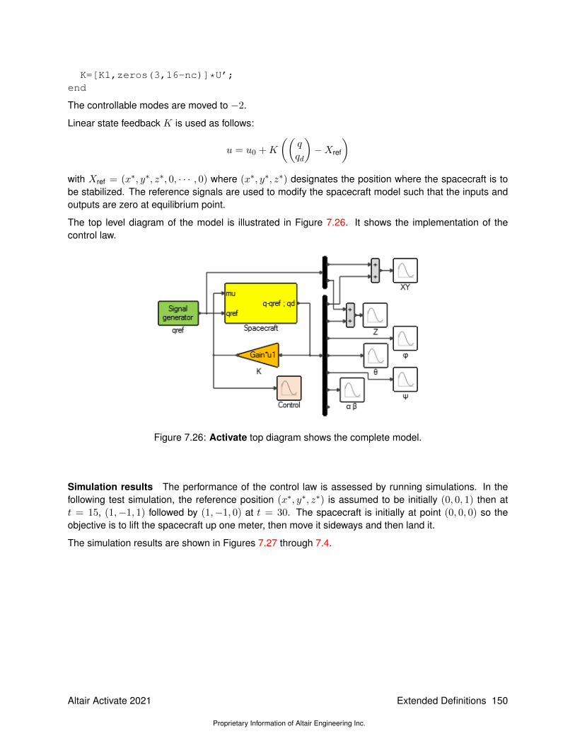
K=[K1,zeros(3,16-nc)]*U’;end
The controllable modes are moved to −2.
Linear state feedback K is used as follows:
u = u0 +K
((qqd
)−Xref
)with Xref = (x∗, y∗, z∗, 0, · · · , 0) where (x∗, y∗, z∗) designates the position where the spacecraft is tobe stabilized. The reference signals are used to modify the spacecraft model such that the inputs andoutputs are zero at equilibrium point.
The top level diagram of the model is illustrated in Figure 7.26. It shows the implementation of thecontrol law.
Figure 7.26: Activate top diagram shows the complete model.
Simulation results The performance of the control law is assessed by running simulations. In thefollowing test simulation, the reference position (x∗, y∗, z∗) is assumed to be initially (0, 0, 1) then att = 15, (1,−1, 1) followed by (1,−1, 0) at t = 30. The spacecraft is initially at point (0, 0, 0) so theobjective is to lift the spacecraft up one meter, then move it sideways and then land it.
The simulation results are shown in Figures 7.27 through 7.4.
Altair Activate 2021
Proprietary Information of Altair Engineering Inc.
Extended Definitions 150

Figure 7.27: The altitude z follows the reference trajectory by going from 0 to 1 and then back to 0.
Figure 7.28: The XY position of the spacecraft follows the reference by going from (0, 0) to (−1, 1).
151 Extended Definitions
Proprietary Information of Altair Engineering Inc.
Altair Activate 2021

Figure 7.29: The control signals are illustrated here: F − F0, σ and τ .
Figure 7.30: The angles α and β corresponding to the universal joint.
Altair Activate 2021
Proprietary Information of Altair Engineering Inc.
Extended Definitions 152

Figure 7.31: The simulation shows a drift in the ψ signal, which is not controllable and thus cannot bebrought to zero. This however is not an issue.
AppendixL =
(((−0.5 α
2l1
2m1 + 0.5 β
2l0
2m0
)cos(φ)
2+ (0.5 I0x − 0.5 I0z) φ
2cos(α)
2+ (0.5 I1z
− 0.5 I1x) φ2
cos(β)2+ (−0.5 I0x + 0.5 I0z − 0.5 I1z + 0.5 I1x) φ
2)cos(θ)
2+
(α2l1
2
m1 − β2l0
2m0
)cos(φ)
2+ (−0.5 I0x + 0.5 I0z) θ
2cos(α)
2+ (−0.5 I1z + 0.5 I1x)
θ2
cos(β)2 − 0.5 α
2l1
2m1 + (−0.5 I0z − 0.5 I1x + 0.5 I1z + 0.5 I0x) θ
2
+ 0.5 β2l0
2m0
)cos(ψ)
2+
((cos(φ)
2sin(θ) β l0
2m0 ψ +
(− cos(α) l1m1 θ
x− sin(α) l1m1 θ z − sin(φ) α l12m1 ψ + l0m0 θ x
)cos(φ) +
((I0x − I0z) θ φ cos(α)
2+ (−I1x + I1z) θ φ cos(β)
2
+ (−I1z + I0z − I0x + I1x) θ φ)sin(ψ) + (I0z − I0x) φ
2sin(α) cos(α)
sin(θ) + (I0z − I0x) ψ φ sin(α) cos(α) + φ β(l0
2m0 + I1x
))cos(θ) + cos(φ)
2α l1
2m1 θ +
((−α2
l12m1 + β
2l0
2m0
)sin(φ)
sin(θ) sin(ψ) +(− cos(α) α l1m1 z − cos(β) l0m0 ψ y + sin(φ)
β l02m0 θ +m1 l1 (x α + g) sin(α) + ψ (z l0m0 sin(β) +m1
y l1)) sin(θ) − cos(β) l0m0 φ y + φ (z l0m0 sin(β) +m1 y l1))
cos(φ) +(cos(α) sin(φ) l1m1 φ x + (I1x − I1z) θ φ sin(β) cos(β)
+(sin(α) l1m1 φ z − l0m0 φ x
)sin(φ)
)sin(θ) + cos(α) sin(φ) l1m1
ψ x +(sin(φ) β l0m0 z + (I1x − I1z) ψ θ sin(β)
)cos(β)
+(sin(α) l1m1 ψ z + (−g + β y) l0m0 sin(β) − l0m0 ψ x
)sin(φ)
+ I0x α θ)cos(ψ) +
(((−0.5 ψ
2+ 0.5 α
2)l1
2m1 − 0.5 l0
2m0 ψ
2)
cos(φ)2+ (0.5 I0x − 0.5 I0z) φ
2cos(α)
2+ (I1x − I1z) φ
2cos(β)
2+ (0.5 I1z − 0.5 I1x)
φ2)cos(θ)
2+
(− sin(ψ) cos(φ)
2sin(θ) α l1
2m1 ψ + ((− cos(β) l0m0
θ y − sin(φ) β l02m0 ψ + θ (z l0m0 sin(β) +m1 y l1)
)sin(ψ) + (−g − x α) l1m1 cos(α) + (g − β y) l0m0 cos(β) +
(−l1
2m1
ψ θ − l02m0 ψ θ
)sin(φ) + sin(β) β l0m0 z − sin(α)
α l1m1 z) cos(φ) +((−I1x + I1z) φ
2sin(β) cos(β) sin(θ) + (−I1x + I1z)
ψ φ sin(β) cos(β) +(−α l1
2m1 − I0x α
)φ)sin(ψ)
− cos(α) sin(φ) l1m1 φ z + φ sin(φ) (m1 x sin(α) l1 + y sin(β) l0m0
+ z l0m0 cos(β))) cos(θ) +(sin(ψ) β l0
2m0 θ +
(0.5 l1
2θ2
− 0.5 α2l1
2)m1 + 0.5 β
2l0
2m0 + 0.5 l0
2m0 θ
2)cos(φ)
2+
(((cos(α) l1m1 ψ
x + cos(β) β l0m0 z − sin(φ) α l12m1 θ + sin(α) l1m1 ψ
z + (−g + β y) l0m0 sin(β) − l0m0 ψ x)sin(θ) − l0m0 φ x
+ cos(α) l1m1 φ x + sin(α) l1m1 φ z)sin(ψ) +
(− cos(α) l1m1 θ
z + θ (m1 x sin(α) l1 + y sin(β) l0m0 + z l0m0 cos(β)))sin(θ)
)cos(φ) +
(((I0z − I0x) θ φ sin(α) cos(α) + cos(β) sin(φ) l0m0 φ
y +(−l1m1 φ y − sin(β) l0m0 φ z
)sin(φ)
)sin(θ) + (sin(φ)
α l1m1 z + (I0z − I0x) ψ θ sin(α))cos(α) + cos(β) sin(φ) l0m0
ψ y +((−g − x α) l1m1 sin(α) − l1m1 ψ y − sin(β) l0m0
ψ z)sin(φ) + I1x β θ
)sin(ψ) +
((I0z − I0x) ψ φ
cos(α)2+ (−I1x + I1z) ψ φ cos(β)
2+ φ ψ
(l0
2m0 + l1
2m1 + I0x + I1x
))sin(θ) +
((−0.5 I0x + 0.5 I0z) φ
2+ (0.5 I0x − 0.5 I0z) θ
2+ (−0.5 I0x + 0.5 I0z)
ψ2)cos(α)
2+
((0.5 I1z − 0.5 I1x) φ
2+ (0.5 I1z − 0.5 I1x) ψ
2)cos(β)
2
+(0.5 l0
2m0 + 0.5 l1
2m1 + 0.5 I0x + 0.5 I1x
)φ2+
((0.5 ψ
2+ 0.5 α
2)l1
2 − g z + 0.5 x2
+ 0.5 y2+ 0.5 z
2)m1 + (0.5 I0z + 0.5 I1x) θ
2+
(0.5 l0
2ψ
2 − g z + 0.5 x2+ 0.5 y
2
+ 0.5 z2)m0 + (0.5 I0x + 0.5 I1x) ψ
2+ 0.5 I0x α
2+ 0.5 I1x. β
2
153 Extended Definitions
Proprietary Information of Altair Engineering Inc.
Altair Activate 2021

Altair Activate 2021
Proprietary Information of Altair Engineering Inc.
Extended Definitions 154

Chapter 8
Altair Activate Libraries
In Activate, libraries are self-contained repositories that essentially provide the application with newblocks. But, beyond just blocks, a library provides also (OML) functions that the user can use within hisscripts.
8.1 Library structure
A library in Activate can be described by the following structure:
Figure 8.1: Representation of a typical library in Activate
• key: The library is identified by its key. The key is generated automatically by Activate in thefile _key. This file is updated every time the library is edited after a release; a new version of
155 Extended Definitions
Proprietary Information of Altair Engineering Inc.
Altair Activate 2021

the library is created. The first line of the _key file defines the current version ID, the other linesdefines the IDs of the old versions. This file should not be manually edited, as this could alter thelibrary.
• loader: The blocks of the library are loaded into Activate through the loader.oml file. This file isautomatically generated, it must not be edited.
• libinit: The library can add to the Activate environment palettes, menus and functions. The usercan edit the libinit.oml file to perform such actions.
• palette(s): The palettes of the library can be any scm file loaded as palette in the libinit file. Thepalette browser shows only the blocks. The links and annotations are discarded.
• block : A block in Activate is defined by the interface file (SCB) and the simulation functions.The block interface files can be organized hierarchically under the condition that the folder thatcontains the SCB file must have the same name as the SCB. The Hierarchical path defines thereference path of the block, it is relative to the library top level. The simulation functions of theblock must be inside the _sim folder of the library. The relative paths of the simulation functionsmust be equivalent to the ones defined in the SCB file.
• icons: Icons of the blocks should be defined inside the _icons folder of the library.
• documentation: The block documentation is generated inside _doc folder.
The image below can summarize the library structure:
Figure 8.2: Description of a library folder in Activate
Altair Activate 2021
Proprietary Information of Altair Engineering Inc.
Extended Definitions 156

8.2 Block structure
In a Activate library a block is defined by several files.
• SCB: The file describes the graphics part of the block. It contains also the parameters definitionand the evaluation part of the block. This file is generated by selecting a block and using the menuFile/Save Selected. The block can also be a masked Super Block, or an atom block. Creatingan atom block can be done through the menu Tools/Block Builder.
• OML: The file is generated from the SCB, it should not be edited. It is used during the evaluationphase of the simulation.
• XML: The file is used for the documentation, the skeleton of that file is generated automaticallyfrom the SCB file. This file should be completed by the block creator.
• HTML: The file is generated from the XML file, it is pushed under _doc folder.
As an example, the image below illustrates the structure of the constant block in the Activate library.
Figure 8.3: Constant block folder content
A block can have one or many simulation functions, they are considered to be C entry point functions.They are defined under the _sim folder of the library. A library creator can decide to either ship theC code or not, but it is mandatory to ship the static and the shared libraries. If a simulation functiondepends on a third party library, the shared and static library of that third party must be delivered underthe _bin folder of the library.
Figure 8.4: Constant block: View of the simulation folder content
8.3 Palette
The palette is the way to expose the blocks of a library to the user. It is very similar to a model. It canbe edited by Activate as any other model. A non masked Super Block in a palette is used to createhierarchy in the palette browser. A masked Super Block is seen in the palette browser as a block. Sincethe Block Diagram Editor manipulates palettes as models, the extension of the palette file is scm.
A library can have several palettes, and in contrast, some libraries may not need to expose any block,in which case the library does not have any palette.
157 Extended Definitions
Proprietary Information of Altair Engineering Inc.
Altair Activate 2021

Since the palettes are the interface of the library, the user can choose the blocks to be exposed. Someof the blocks that are considered as “support” blocks, may not be place into a palette. However, userscan still access such blocks through the menu File/Libraries/Insert Block From Library.
A palette does not need to be associated with any library. The user can create his own palette basedon the existing blocks. He can, for example, create his favorite palette to host his most used blocks. Inthat case, the user will create a model and use the menu File/Libraries/Save as Palette. This paletteis then loaded and exposed under the Personal page of the Library Browser.
When a library is Uninsulated, files are removed. The palettes loaded by that library should be removedfrom the palette browser. To remove Personal palettes, the user can use the menu File/Libraries/RemovePalette.
8.4 Library creation
Activate offers two ways from creating and editing a library:
• Library Manager: Activate provides a GUI to help the user create and edit his libraries.
• OML functions: Activate provides OML functions to allow the user to create and edit his libraries.
Note that the Library Manager provides an easy but limited way to edit the library. For advanced users,the use of (OML) functions is recommended.
8.4.1 Library Manager
Figure 8.5: Library Manager
The Library Manager allows the user to:
• create a new library: The user must define the name and the path of the library. Note that uponcreation, the library is also installed.
Figure 8.6: Create Library
Altair Activate 2021
Proprietary Information of Altair Engineering Inc.
Extended Definitions 158
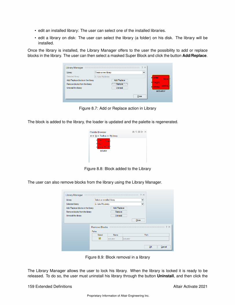
• edit an installed library: The user can select one of the installed libraries.
• edit a library on disk: The user can select the library (a folder) on his disk. The library will beinstalled.
Once the library is installed, the Library Manager offers to the user the possibility to add or replaceblocks in the library. The user can then select a masked Super Block and click the button Add/Replace.
Figure 8.7: Add or Replace action in Library
The block is added to the library, the loader is updated and the palette is regenerated.
Figure 8.8: Block added to the Library
The user can also remove blocks from the library using the Library Manager.
Figure 8.9: Block removal in a library
The Library Manager allows the user to lock his library. When the library is locked it is ready to bereleased. To do so, the user must uninstall his library through the button Uninstall, and then click the
159 Extended Definitions
Proprietary Information of Altair Engineering Inc.
Altair Activate 2021

button Lock. When the library is locked, the user cannot add or remove any block from it.
The Library Manager gives the possibility to the user to edit a locked library through the button Unlock.This feature will create a new version of the library, a new key is created in the _key file, the blocks areupdated and the palette is regenerated, it references the blocks with the new key.
Figure 8.10: Example of library keys
Figure 8.11: Library key used (referenced) in a block
The models and the scripts that use the old version of the library will still work. The user must makesure that his library is backward compatible. He cannot remove any block from the library. He cannotchange the hierarchical organization of the blocks. He cannot remove any exposed OML function. Fora given block, he cannot remove any parameter.
8.4.2 OML functions
Activate provides OML functions to manipulate explicitly the libraries.
Create library
This function creates a skeleton of the library on the disk. It generates a new key and assigns that keyto the library. The arguments of that function are the name of the library and the path where the librarymust be created.
vssCreateEmptyLibrary(’mylib’,’x:/Libraries’);
Adding blocks
The user can use the menu Tools/Block Builder to create his blocks. The block will be created andinserted in the current model. To add the block to the library the user can select the created block andcall the following functions:
blk=bdeGetSelectedBlock(bdeGetCurrentDiagram());vssAddBlockToLibrary(blk,’x:/Libraries/mylib/Level1/MyBlock’);
The user can also use the Block Diagram Editor APIs to create the block.
Refresh library
After populating the library with the blocks, the refresh function generates the OML functions used bythe evaluator, the XML files used to generate the documentation, and the libraries used by the simulator.
Altair Activate 2021
Proprietary Information of Altair Engineering Inc.
Extended Definitions 160

This function generates also the loader of the library. The argument of that function is the path of thelibrary.
vssRefreshLibrary(’x:/Libraries/mylib’);
The library is now ready to be used.
Note: Every time the user adds a block to his library, he must refresh the library and execute the loaderso that the new block is taken into account.
Generate palette
Activate offers several methods to create a palette.
• The user can generate the palette automatically from the library; In this case the palette containsall the blocks of the library. He can then edit the palette to remove or add blocks. The palettesof a library must contain only blocks from the library or from the System (Activate) library. In thiscase he can use the function
vssGeneratePalette(’x:/Libraries/mylib’);
• The user can generate the palette manually. In this case, he can use the Block Diagram Editorsince a palette is in essence a model. Steps are: open a new model, add new block(s) to themodel through the menu File/Libraries/Insert Block From Library and finally save the model inthe library.
Add palette
Once the palettes are generated we must edit the libinit.oml file by adding the AddPalette function. Thatfunction adds the palettes of the library to the toolbox page.
vssAddPalette([libPath, ’/mylib.scm’]);
where libPath is the path of the library.
Note: to make the library movable, use the variable libPath defined in libinit.oml instead of hard codingthe path of the library.
Install library
This function installs the library in the Activate environment. It does not change the location of thelibrary on the disk.
vssInstallLibrary(’x:/Libraries/mylib’);
The library is now installed, the palettes are added to the palette browser and the user can start usingthe library.
Uninstall library
The user can uninstall the library. The palettes that come with the library will be removed from theLibrary Browser. Once a library is uninstalled, users cannot run any model that uses blocks from that
161 Extended Definitions
Proprietary Information of Altair Engineering Inc.
Altair Activate 2021

library.
vssUninstallLibrary(’x:/Libraries/mylib’);
Document library
The user can start documenting his blocks. He has to edit the XML file corresponding to each block.The fields that are already filled must not be changed. He can give for example more information aboutthe block in the description section. Once the blocks are documented, he can use the following functionto update the HTML pages.
vssGenerateDocumentation(’x:/Libraries/mylib’);
Lock library
The library is now ready to be delivered. The user must lock the library before releasing. Once lockeduser cannot add any block or function to the library. The library is now read-only.
vssLockLibrary(’x:/Libraries/mylib’);
Unlock library
As a library creator, user can still edit his library after it has been locked. In this case he must, first,unlock the library.
A new key is generated indicating that this is a new version of the library. The new version of the librarymust be backward compatible. He cannot remove any block from the library. He cannot change thehierarchical level of the blocks. He cannot remove any exposed OML function. For a given block, hecannot remove any parameter.
vssUnlockLibrary(’x:/Libraries/mylib’);
Altair Activate 2021
Proprietary Information of Altair Engineering Inc.
Extended Definitions 162

Chapter 9
Altair Activate blocks
An Activate Model is an interconnection of blocks. Most Activate users do not need to develop newblocks because Activate provides a large number of blocks through different palettes. Advanced usershowever may need to develop new specialized blocks. These blocks may be placed in new libraries anddistributed to other users.
Blocks in Activate may be constructed based on other blocks. A masked Super Block for examplebehaves almost like any other block in the Block Diagram Editor (BDE); the only difference is that thediagram inside the Super Block can be visualized and edited only using the “Enter Masked Super Block”contextual menu item1.
A block may also be defined through a diagram inside, similarly to a Super Block, but without anyassociated graphical information. These blocks are called programmable super blocks. The content ofthe block is defined via OML scripts using special APIs instantiating and connecting blocks to definethe inside diagram. At the BDE level, programmable super blocks are indistinguishable from basicblocks. In the absence of graphical information concerning the inside diagram, the “Enter MaskedSuper Block” operation is not available. In fact this operation cannot apply even if graphical informationwere available since the content of a programmable super block may depend on block parameters. Forexample a block parameter may define the number of times a structure is repeated in the diagram. Theparameter values not necessarily being available in the BDE, the diagram structure is not even known.
A basic block defines its behavior directly through a simulation function. Simulation functions are de-fined as C functions in most cases but they can also be defined in OML. Simulation functions can bedeveloped first for CCustomBlock or OMLCustomBlock and tested before being used in the definitionof a new basic block.
The construction of simulation functions for basic blocks is discussed in the next section. Once thesimulation function is developed, the construction of a new block is greatly simplified using the Activatetool Block builder tool. Block builder is presented in Section 9.2.
9.1 Block simulation function
A block communicates with other blocks via the regular input and output ports and activation inputand output ports. Signals associated with regular input and output ports can be of type matrix of real,
1In case of a library block, the block must be first inlined to enter the Super Block
163 Extended Definitions
Proprietary Information of Altair Engineering Inc.
Altair Activate 2021
complex or integer data types. The activation input and output ports, on the other hand, transmit onlyevents (which are also called activations).
A block can have several regular and activation input and output ports. A block can also have continuous-time, discrete-time states, and zero-crossing surfaces. Of course a block does not need to have all ofthese elements.
The behavior of an Activate block is basically governed by the way it is activated. The block is activatedwhen it receives activation on its activation input ports. If the block does not have input activation, it canbe activated by inheritance. In this case, the activation input ports are added by the Activate compilerto the block. The block can also be defined as being Always active.
A block can be activated in many different ways. In the following a number of scenarios are presented.
Discrete-time activation, or events When a block is activated by an event on its activation input port,it can update its regular outputs:
y(te) = foutput(te, x(t−e ), z(t−e ), u(te), nevprt,m, phase, p)
where te is the activation or event time, x(t−e ) and z(t−e ) represent continuous-time and discrete-timestates just before the occurrence of the event. y and u are output and input of the block. nevprt isa positive integer indicating by which activation input port the block has been activated. m, phase, pare mode, simulation phase, and parameters of the block respectively. mode and simulationphase will be discussed later.
If the block has output activation ports, it can program events on them by defining the delay time (whichcan be zero) on each activation output port:
tevo = fevent(te, x(t−e ), z(t−e ), u(te), nevprt,m, phase, p).
tevo is a vector with the same size that the number of activation output ports. Once programmed, iftevo[i] is positive, an event is programmed at time te + tevo[i] at activation output port i+ 1.
The continuous-time and discrete-time states of the block, if present, can also be updated at eventtimes.
[x(te), z(te)] = fdiscrete(te, x(t−e ), z(t−e ), u(te), nevprt,m, phase, p).
Continuous-time activation If the source of the activation is always active, then activation occursover time interval and not at specific time instants similar to discrete-time events. In Continuous-timeactivation, the output computation can be represented with
y(t) = foutput(t, x(t), z(t), u(t),m, phase, p)
During a continuous-time activation, no state update and no event-programming is performed. Discrete-time states z, mode variables and simulation phase stay unchanged. On the other hand, thecontinuous-time state follows the differential equation.
x(t) = fcontinuous(t, x(t), z(t), u(t),m, phase, p)
Altair Activate 2021
Proprietary Information of Altair Engineering Inc.
Extended Definitions 164
Zero-crossing function and mode variables Activate provides several numerical solvers, includingfixed step-size and variable step-size solvers such as Lsoda and Radau. Variable step-solvers adjustthe integration step size during the integration to provide a faster simulation without compromising theprecision in the solution.
If the differential equation represented by the diagram is not smooth enough, the variable-step solversreduce the step-size to cope with the non-smoothness or even discontinuity. If foutput or fcontinuous is notsmooth (continuously differentiable) at some points, then mode variable is used in such way as to makesure the numerical solver never encounters these discontinuity points inside the integration interval.Consider the following example:
y =
u if u ≥ 0−u otherwise
This function implements the absolute value function and is not differentiable at u = 0. In this case, amode variable can be defined to specify at the start of the integration period whether u is positive. Tomake sure the integration stops when sign of u changes, a zero-crossing surface is introduced at zero,here the zero-crossing surface is u = 0. During the integration period (which could end because of thezero-crossing), the output y is computed as follows:
y =
u if m = 1
−u otherwise
Once the zero-crossing is detected, the numerical solver stops and the mode is recomputed; then theintegration continues. The computation of the mode and the zero-crossing surface are performed bythe block. The block can be called in different situations or phases. In some phases, such as duringthe numerical integration, mode variables are fixed and in other phases, modes are updated. Forexample when an event activates the block, mode variables can be updated. The phase variable isnot directly accessible to the user. The user can check if mode variables are fixed or not by using themacro isModeFixed(block).
When a variable step solver integrates a model, it may happen that a time interval be repeated severaltimes till the solver accepts the step and starts another step. In most situations users need not worryabout these intermediate repeated calls, but in some cases, e.g., when the output of the block is dis-played, these calls should be ignored. In order to filter these calls, the macro isinTryPhase(block)is used. This macro uses the phase variable to find out whether the call should be ignored. It is impor-tant to indicate that mode variables are used only when the numerical solver is variable-step.
Zero-crossing functions can also be used to generate discrete-time events. Once a zero-crossing sur-face function inside a block crosses zero, the block is activated with a nevprt = −1, i.e., at this eventtime te, fdiscrete is called with nevprt = −1. This type of activation is used, e.g., in modeling a simplebouncing ball that will be presented later.
9.1.1 Simulation function implementation
The simulation function is normally written in C, but can also be written in OML. This function definesthe behavior of the block during the simulation.
The simulation function is called by the simulator with two arguments: a C structure containing blockinformation (vss_block) and a integer value called flag. The calling sequence is as follows:
MyNewBlock(vss_block *block, int flag)
165 Extended Definitions
Proprietary Information of Altair Engineering Inc.
Altair Activate 2021

The calling arguments will be discussed in the following sections.
vss_block structure
The vss_block structure is a hierarchical C structure providing access to the block parameters andvariables.
struct vss_block ....BlockInputX input;BlockOutput output;BlockEventInput evinput;BlockEventOutput evoutput;SimFunction sim;BlockState state;BlockDState dstate;BlockODState odstate;BlockConstraint constraint;BlockRpar rpar;BlockIpar ipar;BlockOpar opar;BlockZcross zcross;BlockMode mode;SCSPOINTER_COP *work;SCSINT_COP ajac;BlockName name;SCSINT_COP dept;SCSSTRING_COP blocktype;
SCSPOINTER_COP simulatorVars;.....
;
Note that vss_block is a hierarchical C structure. For example, BlockOutput is another structuredefined as:
typedef struct ....SCSINT_COP nout;SCSINT_COP outdim;SCSINT_COP *outsz;SCSINT_COP *outtyp;SCSPOINTER_COP *outptr;....
BlockOutput;
In the above structure, the standard C data-types, are redefined, for example:
#define SCSREAL_COP double
The complete list of these data-types are given in 9.1.1.
Altair Activate 2021
Proprietary Information of Altair Engineering Inc.
Extended Definitions 166

The block structure is quite complex; in order to facilitate accessing the embedded data, a large num-ber of macros are provided. All access to this structure must be made through these macros. Mostcommonly used macros are presented in Sections 9.1.3 and 9.1.4. As an example, in order to accessthe data-type of the second block output, the user can use the following macro:
int *odt=GetOutType(block,2);
Flag
Flag is an integer (or more precisely an enumeration) value indicating the job for which the block hasbeen called by the simulator. Blocks may be called with different flags to perform different operations.For example the block can be called with flag= VssFlag_OutputUpdate (= 1), to update itsoutputs or can be called with flag= VssFlag_Derivatives (= 0), to provide the state derivatives.
The list if all flags and their meanings are provided below.
• VssFlag_Initialize: The block is called for the first time at the beginning of the simulationwith this flag where initialization issues can be done. Operations such as opening data files,initializing a TCP/IP socket, or dynamic memory allocation can be done in this flag call. Althoughcontinuous-time and discrete-time states have already been initialized, they can be reinitialized (ifneeded). In this flag, input and output of the block are not available, hence cannot be initializedor read. Each block is called with this flag only once at the beginning of the simulation.
• VssFlag_Terminate: Once the simulation is finished, or stopped due to an error or on theuser request, the simulator calls the blocks once at final time with this flag. This flag is useful,e.g., for closing a file or a socket that has been opened in flag VssFlag_Initialize.
• VssFlag_OutputUpdate: When the block is called with this flag, the simulator is requestingthe output(s) of the block. The block should compute the outputs as a function of time, inputs,nevprt2, and internal states. These values should be obtained from the block structure (thefirst argument of the simulation function). The computed output should be written in the blockstructure using appropriate macros. Note that if the block contains modes3, then the output maybe computed as a function of whether modes are fixed or relaxed; in some cases the call shouldbe ignored. In this case isModeFixed(block) and isinTryPhase(block) macros maybe used.
• VssFlag_StateUpdate: When the simulator calls the blocks with this flag, it means thatan event has activated the block (nevprt>0) and the block can update is discrete-time andcontinuous-time states. The activation event may also be due to a zero-crossing event happenedinside the block (an internal event), in which case (nevprt=-1). When this happens, the jroot4
vector indicates the surface that has crossed and the direction of crossing. If ith entry of jrootis +1 (respectively -1), the the ith surface has crossed zero with a positive (respectively negative)slope. If it is zero, i-th surface has not crossed zero.
• VssFlag_Derivatives: When the block is called with this flag, the simulator requests theblock to provide the continuous-time state time derivatives (x)5. The simulation function shouldcompute x in the address provided by the block for this purpose. If the block is implicit, i.e., the
2accessible by macro GetNevIn(block)3accessible by macro GetModePtrs(block)4accessible by macro GetJrootPtrs(block)5accessible by macro GetDerState(block)
167 Extended Definitions
Proprietary Information of Altair Engineering Inc.
Altair Activate 2021

dynamics of the block is represented by a DAE, the block should compute the residual6 in thecorresponding address.
• VssFlag_ZeroCrossings: When the block is called with this flag, the simulator requeststhe block to provide its zero-crossing surfaces. Variable-step numerical solvers of Activateassume model smoothness. This means that the behavior of blocks, which contain or affectcontinuous-time states of the model must be smooth, or at least piecewise smooth. In case ofnon-smoothness, the points of discontinuity must be specified in such a way that the solver can,if needed, issue a cold restart when going though such points. An example of such a block is theABS block. The absolute value function is smooth except at zero, where it is not differentiable.In this case, we say that absolute value block has two modes: one where the output equals theinput, and one where the output is the negative of the input. A block may have many differentmodes. The point of non-smoothness or discontinuity is represented by a zero-crossing, and themode is updated after such a crossing occurs. The VssFlag_ZeroCrossings flag is usedboth for evaluating the zero-crossing function and returning the zero-crossing vector7 and settingthe mode variables. Mode setting is done only when isModeFixed(block) is False. Note thatthe block may have more zero-crossing than modes. For example, the Zero-cross block whichgenerates an event when its input crosses zero, has one zero-crossing surface, but no mode.
• VssFlag_EventScheduling: When the block is called with this flag, it means that the blockcan program a new event at one or more of its output activation ports. After this call, the simulatorupdates its event scheduler. An event can also be programmed after an internal zero-crossing.In this case, the block can use the jroot vector.
• VssFlag_Reinitialize: When the simulator calls the block with this flag, the block is allowedto reset its continuous-time state as a function of its input values.
• VssFlag_ReinitializeImplicit: In implicit models, after event leading to restarting thesolver, the implicit blocks are called with this flag allowing blocks updating states and state deriva-tives.
• VssFlag_Projection: If a block dynamics is represented by an ODE with algebraic con-straints, the simulator calls the block with this flag to either compute the projection update or theresidual of constraints. The type of constraint is either CONSTRAINT or PROJECTION. If themodel contains blocks with constraints, the number of constraints should be given by this macroGetNConstraint(block). Note that only the CPODE solver can be used to integrate thesetype of models.
• VssFlag_Jacobians: When the block is called with this flag, the simulator requests the blockto provide the analytical Jacobian matrix of the model. The block is called with this flag only if theblock informs the simulator by setting SetAjac(block,1) in flag=VssFlag_Initialize.
• VssFlag_GotoPause: Before stopping the simulation and going to pause, the block is calledfor the last time to perform necessary jobs if needed, for example flushing temporary data intofile.
• VssFlag_ReturnFromPause: After returning from the pause, the blocks are called with thisflag before resuming the simulation.
6accessible by macro GetResState(block)7accessible by macro GetGPtrs(block)
Altair Activate 2021
Proprietary Information of Altair Engineering Inc.
Extended Definitions 168

Flag calling sequence in blocks
The simulator invokes the blocks with specified flag to perform a job or a model update. In or-der to instantiate a block in the simulator before any subsequent call, the simulator calls all blockswith flag= VssFlag_Initialize. Just before finishing the simulation, all blocks are called withflag= VssFlag_Terminate to inform the block that this is the last call from the simulator. A simpleflowchart has been given in Fig.9.1.
Figure 9.1: Simple flowchart indicating different stages of a simulation and different flag by which ablock can be called.
169 Extended Definitions
Proprietary Information of Altair Engineering Inc.
Altair Activate 2021
Data-type supported in blocks
Signals in Activate can be matrices of various data-types. The data-type of input and output of a blockmay either be defined and fixed by the block or be inherited from data-type of other connecting blocks.
In general a block supporting multiple data types should provide a different simulation function for eachdata type. But in some cases it is possible to avoid this by using a single simulation function. For that,the data types and sizes of the parameters, states, inputs and outputs are made available inside thesimulation function via specific macros. For example GetInType(block,n) returns the data-type ofnth input port. The returned data-type can be one of these enumeration values.
• SCSREAL_N: double data-type ID
• SCSCOMPLEX_N: complex data-type ID
• SCSINT32_N: int32 data-type ID
• SCSINT16_N: int16 data-type ID
• SCSINT8_N: int8 data-type ID
• SCSUINT32_N: unsigned int32 data-type ID
• SCSUINT16_N: unsigned int16 data-type ID
• SCSUINT8_N: unsigned int8 data-type ID
• SCSBOOL_N: Boolean data-type ID
• SCSSTRING_N: string data-type ID
The corresponding types that can be used in the simulation function are:
• SCSREAL_COP: double data-type
• SCSCOMPLEX_COP: complex data-type
• SCSINT32_COP: int32 data-type
• SCSINT16_COP: int16 data-type
• SCSINT8_COP: int8 data-type
• SCSUINT32_COP: unsigned int32 data-type
• SCSUINT16_COP: unsigned int16 data-type
• SCSUINT8_COP: unsigned int8 data-type
• SCSBOOL_COP: Boolean data-type
• SCSSTRING_COP: string data-type
Users are encouraged to use these data-type instead of using directly C data-types in the definition ofsimulation functions.
Feedthrough information in blocks
The feedthrough is a block property that specifies the input-output dependency of the block. Thisproperty must be specified when a new block is constructed (including for blocks realized by customblocks). Specifically the feedthrough property is a vector of size equal to the number of block inputs.
Altair Activate 2021
Proprietary Information of Altair Engineering Inc.
Extended Definitions 170

The ith entry of the vector indicates whether or not the block outputs depend "directly" on the ith inputvalue. Consider a Gain block with gain G, input u and output y (one input, one output) realizing:
y = Gu
In this case the output depends directly on the input (unless G is identically zero), so the Gain block ingeneral has feedthrough property (more specifically its input has it). Now consider an integrator blockwith input u, output y and state x:
x = uy = x
In this case the output y does not directly depend on the input u. The integrator block (its input inparticular) does not have feedthrough property. The feedthrough property should be provided correctlyotherwise the Activate compiler cannot compute proper scheduling. A scheduling error may occur ifa true feedthrough property is erroneously set to false. On the other hand, specifying a feedthroughproperty to be true when it is not can lead to a non-existing algebraic loop error detected by the compiler.The algebraic loop error occurs when the diagram contains a path looping through ports having allfeedthrough properties. In that case the blocks cannot be scheduled by the compiler. Even if there areways to "break" algebraic loops (in particular using the Loopbreaker block), it is better not to introducenon-existing ones by properly defining the feedthrough properties of new blocks. For end users, learningabout this property is useful for dealing with algebraic loop errors.
9.1.2 Examples
In this section in order to illustrate the way a simulation function is written, several examples are given.
Simplified Gain block
Consider a Gain block that multiplies the input matrix by a matrix gain value and puts the results at theblock output. Here is the simulation function of this block.
#include "vss_block4.h"
VSS_EXPORT void SimpleGainBlock (vss_block *block,int flag)
if (flag==VssFlag_OutputUpdate)SCSREAL_COP *u=GetRealInPortPtrs(block,1);int ru=GetInPortRows(block,1);int cu=GetInPortCols(block,1);
SCSREAL_COP *y=GetRealOutPortPtrs(block,1);int ry=GetOutPortRows(block,1);int cy=GetOutPortCols(block,1);
SCSREAL_COP *Gain=GetRealOparPtrs (block,1);int rowGain=GetOparSize(block,1,1);int colGain=GetOparSize(block,1,2);
171 Extended Definitions
Proprietary Information of Altair Engineering Inc.
Altair Activate 2021
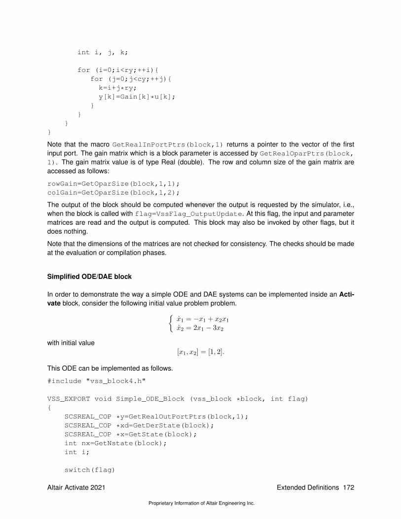
int i, j, k;
for (i=0;i<ry;++i)for (j=0;j<cy;++j)
k=i+j*ry;y[k]=Gain[k]*u[k];
Note that the macro GetRealInPortPtrs(block,1) returns a pointer to the vector of the firstinput port. The gain matrix which is a block parameter is accessed by GetRealOparPtrs(block,1). The gain matrix value is of type Real (double). The row and column size of the gain matrix areaccessed as follows:
rowGain=GetOparSize(block,1,1);colGain=GetOparSize(block,1,2);
The output of the block should be computed whenever the output is requested by the simulator, i.e.,when the block is called with flag=VssFlag_OutputUpdate. At this flag, the input and parametermatrices are read and the output is computed. This block may also be invoked by other flags, but itdoes nothing.
Note that the dimensions of the matrices are not checked for consistency. The checks should be madeat the evaluation or compilation phases.
Simplified ODE/DAE block
In order to demonstrate the way a simple ODE and DAE systems can be implemented inside an Acti-vate block, consider the following initial value problem problem.
x1 = −x1 + x2x1x2 = 2x1 − 3x2
with initial value[x1, x2] = [1, 2].
This ODE can be implemented as follows.
#include "vss_block4.h"
VSS_EXPORT void Simple_ODE_Block (vss_block *block, int flag)
SCSREAL_COP *y=GetRealOutPortPtrs(block,1);SCSREAL_COP *xd=GetDerState(block);SCSREAL_COP *x=GetState(block);int nx=GetNstate(block);int i;
switch(flag)
Altair Activate 2021
Proprietary Information of Altair Engineering Inc.
Extended Definitions 172
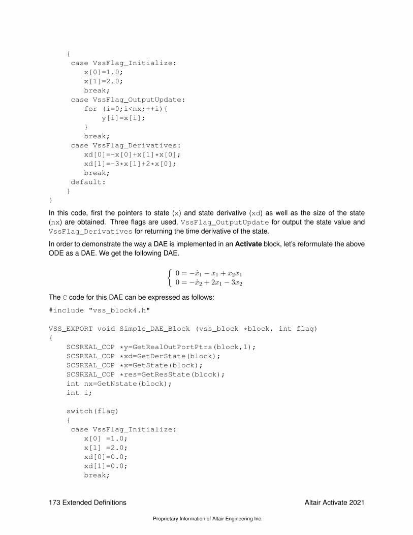
case VssFlag_Initialize:
x[0]=1.0;x[1]=2.0;break;
case VssFlag_OutputUpdate:for (i=0;i<nx;++i)
y[i]=x[i];break;
case VssFlag_Derivatives:xd[0]=-x[0]+x[1]*x[0];xd[1]=-3*x[1]+2*x[0];break;
default:
In this code, first the pointers to state (x) and state derivative (xd) as well as the size of the state(nx) are obtained. Three flags are used, VssFlag_OutputUpdate for output the state value andVssFlag_Derivatives for returning the time derivative of the state.
In order to demonstrate the way a DAE is implemented in an Activate block, let’s reformulate the aboveODE as a DAE. We get the following DAE.
0 = −x1 − x1 + x2x10 = −x2 + 2x1 − 3x2
The C code for this DAE can be expressed as follows:
#include "vss_block4.h"
VSS_EXPORT void Simple_DAE_Block (vss_block *block, int flag)
SCSREAL_COP *y=GetRealOutPortPtrs(block,1);SCSREAL_COP *xd=GetDerState(block);SCSREAL_COP *x=GetState(block);SCSREAL_COP *res=GetResState(block);int nx=GetNstate(block);int i;
switch(flag)case VssFlag_Initialize:
x[0] =1.0;x[1] =2.0;xd[0]=0.0;xd[1]=0.0;break;
173 Extended Definitions
Proprietary Information of Altair Engineering Inc.
Altair Activate 2021

case VssFlag_OutputUpdate:for (i=0;i<nx;++i)
y[i]=x[i];break;
case VssFlag_Derivatives:res[0]=-xd[0]-x[0]+x[1]*x[0];res[1]=-xd[1]-3*x[1]+2*x[0];break;
default:
Simplified Counter (inc/dec) block
In this example, we develop a counter block. Whenever an event activates the counter, the counterincrements or decrements its value. The initial value of the counter and the direction of the counter aregiven as block parameters.
#include "vss_block4.h"VSS_EXPORT void Simple_counter_Block (vss_block *block, int flag)
SCSINT8_COP *y=Getint8OutPortPtrs(block,1);SCSINT8_COP initial=*Getint8OparPtrs(block,1);SCSINT8_COP dir =*Getint8OparPtrs(block,2);SCSINT8_COP mem = Getint8OzPtrs(block,1);int nevprt = GetNevIn(block);
if (flag==VssFlag_Initialize)mem[0]=initial;
else if (flag==VssFlag_OutputUpdate) y[0]=mem[0];
else if (flag== VssFlag_StateUpdate) if (nevprt ==1)
if (dir==1)mem[0]++;
elsemem[0]--;
The initial value of the counter is returned by the macro Getint8OparPtrs(block,1). The blockneeds a storage to keep the counter value. We chose OZ storage, which here is a scalar 8-bit integer. Ingeneral OZ is initialized before the simulation phase, but for demonstration purposes we reinitialized itin flag=VssFlag_Initialize. On every block activation with flag=VssFlag_StateUpdate, the
Altair Activate 2021
Proprietary Information of Altair Engineering Inc.
Extended Definitions 174

nevprt is checked to verify if the activation is a discrete event. Then based on the block parameter(dir), the counter is incremented or decremented.
Simplified Counter block with overflow
In the above counter suppose that the block needs to generate an event when the counter over-flows/underflows. In this case, an event needs to be programmed in flag=VssFlag_EventScheduling.
#include "vss_block4.h"VSS_EXPORT void Simple_counter_Block (vss_block *block, int flag)
SCSINT8_COP *y=Getint8OutPortPtrs(block,1);SCSINT8_COP initial=*Getint8OparPtrs(block,1);SCSINT8_COP dir =*Getint8OparPtrs(block,2);SCSINT8_COP mem = Getint8OzPtrs(block,1);int nevprt = GetNevIn(block);double *evout= GetNevOutPtrs(block);
if (flag==VssFlag_Initialize)mem[0]=initial;
else if (flag==VssFlag_OutputUpdate) y[0]=mem[0];
else if (flag== VssFlag_StateUpdate) if (nevprt ==1)
if (dir==1)mem[0]++;
elsemem[0]--;
else if (flag==VssFlag_EventScheduling)
if (nevprt ==1)if (dir==1)
if (mem[0]==127) evout[0]=0.0;
else
if (mem[0]==-128)evout[0]=0.0;
In this counter, when the block is called with flag=VssFlag_EventScheduling, the content of thecounter is checked and based on the counter direction and its value, an immediate discrete event (withzero delay) is generated at its first activation output port.
175 Extended Definitions
Proprietary Information of Altair Engineering Inc.
Altair Activate 2021
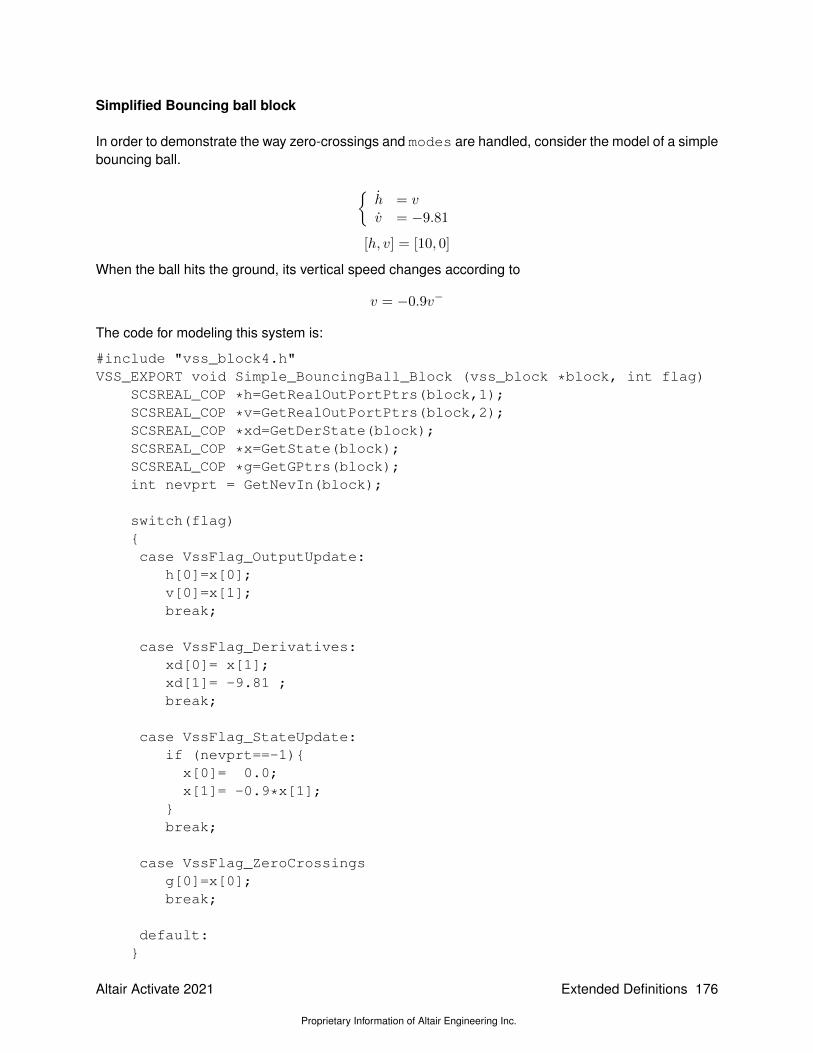
Simplified Bouncing ball block
In order to demonstrate the way zero-crossings and modes are handled, consider the model of a simplebouncing ball.
h = vv = −9.81
[h, v] = [10, 0]
When the ball hits the ground, its vertical speed changes according to
v = −0.9v−
The code for modeling this system is:
#include "vss_block4.h"VSS_EXPORT void Simple_BouncingBall_Block (vss_block *block, int flag)
SCSREAL_COP *h=GetRealOutPortPtrs(block,1);SCSREAL_COP *v=GetRealOutPortPtrs(block,2);SCSREAL_COP *xd=GetDerState(block);SCSREAL_COP *x=GetState(block);SCSREAL_COP *g=GetGPtrs(block);int nevprt = GetNevIn(block);
switch(flag)case VssFlag_OutputUpdate:
h[0]=x[0];v[0]=x[1];break;
case VssFlag_Derivatives:xd[0]= x[1];xd[1]= -9.81 ;break;
case VssFlag_StateUpdate:if (nevprt==-1)x[0]= 0.0;x[1]= -0.9*x[1];
break;
case VssFlag_ZeroCrossingsg[0]=x[0];break;
default:
Altair Activate 2021
Proprietary Information of Altair Engineering Inc.
Extended Definitions 176

The model contains two state variables, one for the height of the ball (h) and another for the velocityof the ball (v). The block has two output ports, the first outputs h and the second, v. A zero-crossingsurface has been used to check whether the ball has hit the ground. Naturally the height of the ball (h)can be used as a zero-crossing surface in the block. When the ball hits the ground, an internal event isgenerated (with nevprt==-1). At this moment, the state variable (h and v) are reset with new values.
Absolute value block
In order to demonstrate the way mode variables are handled in a block, consider a simplifed version ofthe Abs block in Activate. This block computes the absolute value of its input.
y =
u if u ≥ 0−u otherwise
When a variable step-size numerical solver is chosen in Activate, if the output of the Abs block affectscontinuous-time state of the model, mode variable should be used inside the block to handle correctlythe non-smoothness or discontinuity. The absolute value block needs then a zero-crossing surface todetect when the input crosses zero and a mode to handle the discontinuity. The zero-crossing surface isdefined in flag=VssFlag_ZeroCrossings. When the block is called with this flag, the block updatesthe zero-crossing surface and modes.
In order to update the mode variables, the areModesFixed(block) macro is checked, if false,modes can be updated. If the simulator calls the block with flag=VssFlag_OutputUpdate for up-dating the outputs, the block should make use of the mode variable. If the simulator calls the blockwhen areModesFixed(block) is true, the outputs depends on the mode. The code for the simula-tion function of the block is:
#include <vss_block4.h>VSS_EXPORT void simple_abs(vss_block *block,int flag)
SCSREAL_COP *u=GetRealInPortPtrs(block,1);SCSREAL_COP *y=GetRealOutPortPtrs(block,1);SCSREAL_COP *g=GetGPtrs(block);SCSINT32_COP *mode=GetModePtrs(block);int side;
switch(flag)case VssFlag_OutputUpdate:
if (areModesFixed(block)) side=mode[0];
else if (u[0]<0) side=2; else side=1;
if (side==1) y[0]=+u[0];
177 Extended Definitions
Proprietary Information of Altair Engineering Inc.
Altair Activate 2021

else y[0]=-u[0];
break;case VssFlag_ZeroCrossings:
g[0]=u[0];if (!areModesFixed(block))
if(g[0]<0)mode[0]=2;
elsemode[0]=1;
A block to write signals to a file
In this example we demonstrate the way the block input can be written into an ascii file. The input ofthe block is scalar of data type double. The code is:
#include "vss_block4.h"
typedef struct unsigned int index;FILE *pFile;
write2File_t;
#define WS ((write2File_t *) GetWorkPtrs(block))
VSS_EXPORT void write_to_file(vss_block *block,int flag)
switch(flag)
/*---------------------------*/case VssFlag_Initialize:
char *fname=Getint8OparPtrs(block,1);GetWorkPtrs(block)= (write2File_t*)vss_malloc(block,
sizeof(write2File_t) );if (!WS)SetBlockError(block,1);return;WS->index=0;WS->pFile = fopen (fname,"w");if(!WS->pFile) Coserror(block,"Unable to open the file %s\n"
, fname); return;fprintf (WS->pFile, "input data.....\n");
break;/*---------------------------*/
Altair Activate 2021
Proprietary Information of Altair Engineering Inc.
Extended Definitions 178
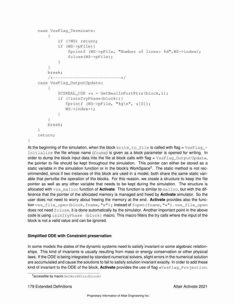
case VssFlag_Terminate:
if (!WS) return;if (WS->pFile)
fprintf (WS->pFile, "Number of lines: %d",WS->index);fclose(WS->pFile);
break;/*---------------------------*/
case VssFlag_OutputUpdate:
SCSREAL_COP *u = GetRealInPortPtrs(block,1);if (!isinTryPhase(block))
fprintf (WS->pFile, "%g\n", u[0]);WS->index++;
break;
return;
At the beginning of the simulation, when the block write_to_file is called with flag = VssFlag_-Initialize the file whose name (fname) is given as a block parameter is opened for writing. Inorder to dump the block input data into the file at block calls with flag = VssFlag_OutputUpdate,the pointer to file should be kept throughout the simulation. This pointer can either be stored as astatic variable in the simulation function or in the block’s WorkSpace8. The static method is not rec-ommended, since if two instances of this block are used in a model, both share the same static vari-able that perturbs the operation of the blocks. For this reason, we create a structure to keep the filepointer as well as any other variable that needs to be kept during the simulation. The structure isallocated with vss_malloc function of Activate. This function is similar to malloc, but with the dif-ference that the pointer of the allocated memory is managed and freed by Activate simulator. So theuser does not need to worry about freeing the memory at the end. Activate provides also the func-tion vss_file_open(block,fname,"w"); instead of fopen(fname,"w"). vss_file_opendoes not need fclose, it is done automatically by the simulator. Another important point in the abovecode is using isinTryPhase (block) macro. This macro filters the try calls where the input of theblock is not a valid value and can be ignored.
Simplified ODE with Constraint preservation
In some models the states of the dynamic systems need to satisfy invariant or some algebraic relation-ships. This kind of invariants is usually resulting from mass or energy conservation or other physicallaws. If the ODE is being integrated by standard numerical solvers, slight errors in the numerical solutionare accumulated and cause the solutions to fail to satisfy solution invariant exactly. In order to add thesekind of invariant to the ODE of the block, Activate provides the use of flag =VssFlag_Projection.
8accessible by macro GetWorkPtrs(block)
179 Extended Definitions
Proprietary Information of Altair Engineering Inc.
Altair Activate 2021

and the CPODE solver. During the simulation the simulator calls the simulation functions of the blockswith constraints with this flag and requests the block to compute the invariant or the projections as afunction of newly computed states. This results in a solution that sticks to the constraints. The followingexample is the standard pendulum model with two invariants. The dynamic model of the pendulum is
x = vxy = vyvx = −x(v2x + v2y − gy)/L2
vy = −y(v2x + v2y − gy)/L2 − g
The first invariant, e.g., ensures that the length of the pendulum remains equal to L throughout thesimulation.
x2 + y2 = L2
xvx + yvy = 0
The code for the simulation function of the pendulum model with constraint preservation follows.
#include "vss_block4.h"#define g 9.81VSS_EXPORT void CBlockFunction(vss_block *block,int flag)
double *xd=GetDerState(block);double *X=GetState(block);double *y=GetRealOutPortPtrs(block,1);int nx=GetNstate(block);int i, ip;
switch(flag)
/*---------------------------*/case VssFlag_Initialize:
SetConstraintKind(block,CONSTRAINT);SetNConstraint(block,2);X[0]=1;X[1]=X[2]=X[3]=0;return;
case VssFlag_Projection:
double x, y, xd, yd;double *corr=GetCorrPtr(block);x = X[0];y = X[1];xd = X[2];yd = X[3];
corr[0]= x*x + y*y - 1.0;
Altair Activate 2021
Proprietary Information of Altair Engineering Inc.
Extended Definitions 180

corr[1]= x*xd + y*yd;return;
case VssFlag_Derivatives:
double x, y, xd, yd, tmp;x = X[0];y = X[1];xd = X[2];yd = X[3];tmp = xd*xd + yd*yd - g*y;
xd[0] = xd;xd[1] = yd;xd[2] = -x*tmp;xd[3] = -y*tmp - g;return;
case VssFlag_OutputUpdate:
for (i=0;i<nx;i++)y[i] = X[i];
return;
default:return;
ODE and DAE blocks providing Analytical Jacobian
In order to solve an ODE/DAE, the numerical variable-step solvers need the Jacobian matrix of theODE/DAE. In Activate, the Jacobian matrix can either be computed numerically by the finite differencemethod or can be provided by blocks. In this section, we show the way the Jacobian of a ODE/DAE canbe provided by the block. Consider the following ODE model and its Jacobian matrix is
x = f(x) =
−x1 + x1x22x1 − 3x2
J =∂f
∂x=
[−1 + x2 x1
2 −3
]
The simulation function for this block providing the analytical Jacobian matrix is given below. In flag=VssFlag_-Initialize, the jacobian flag is set to 1 to inform the simulator that the block provides the analytical
181 Extended Definitions
Proprietary Information of Altair Engineering Inc.
Altair Activate 2021

Jacobian. The J vector has been filled with the Jacobian entries in flag VssFlag_Jacobians. Notethat the J matrix is filled column-wise.
#include "vss_block4.h"
VSS_EXPORT void Simple_ODE_Block (vss_block *block, int flag)
SCSREAL_COP *y=GetRealOutPortPtrs(block,1);SCSREAL_COP *xd=GetDerState(block);SCSREAL_COP *x=GetState(block);SCSREAL_COP *J= GetJacobianPtrs(block);int nx=GetNstate(block);int i;
switch(flag)case VssFlag_Initialize:
SetAjac(block,1);return;
case VssFlag_OutputUpdate:for (i=0;i<nx;++i)
y[i]=x[i];break;
case VssFlag_Derivatives:xd[0]=-x[0]+x[1]*x[0];xd[1]=-3*x[1]+2*x[0];break;
case VssFlag_Jacobians:J[0]=-1+x[1];J[1]=2;J[2]=x[0];J[3]=-3;break;
default:
The Jacobian matrix for a DAE is a little different. For the DAE
0 = F (x, x)
the Jacobian Matrix is defined as follows
J = α∂F
∂x+ β
∂F
∂x
Altair Activate 2021
Proprietary Information of Altair Engineering Inc.
Extended Definitions 182

where α9 and β10 values are given by the simulator. As a result the Jacobian matrix for the above DAEwill be
J =
[−α+ αx2 − β αx1
2α −3α− β
]
#include "vss_block4.h"
VSS_EXPORT void Simple_ODE_Block (vss_block *block, int flag)
SCSREAL_COP *y=GetRealOutPortPtrs(block,1);SCSREAL_COP *xd=GetDerState(block);SCSREAL_COP *x=GetState(block);SCSREAL_COP *J= GetJacobianPtrs(block);SCSREAL_COP *alpha=GetAlphaPt(block);SCSREAL_COP *beta =GetBetaPt(block);int nx=GetNstate(block);int i;
switch(flag)case VssFlag_Initialize:
SetAjac(block,1);return;
case VssFlag_OutputUpdate:for (i=0;i<nx;++i)
y[i]=x[i];break;
case VssFlag_Derivatives:xd[0]=-x[0]+x[1]*x[0];xd[1]=-3*x[1]+2*x[0];break;
case VssFlag_Jacobians:J[0]=-alpha[0]+alpha[0]*x[1]-beta[0];J[1]=-2*alpha[0] ;J[2]=alpha[1]*x[0];J[3]=-3*alpha[1]-beta[1];break;
default:
9accessible by macro GetAlphaPt(block)10accessible by macro GetBetaPt(block)
183 Extended Definitions
Proprietary Information of Altair Engineering Inc.
Altair Activate 2021

A simple block for programming an initial event
Consider a simple block with one output event port that generates an event at a time instant spec-ified by a block parameter. In order to generate the event, the block should read the parametervalue using evtime= GetRealOparPtrs(block,1). Events are only programmed at flag==VssFlag_EventScheduling. In order to program this event only once, at the beginning of thesimulation, the isExitInitialization(block) macro can be used. This macro indicates if theinitialization has finished and the simulation is being started. The relative time with respect to the currentsimulation time and the desired event time is defined and set to the evout vector.
#include "vss_block4.h"
VSS_EXPORT void EventGenerateBlock(vss_block *block,int flag)
double *evout =GetNevOutPtrs(block);double *evtime=GetRealOparPtrs(block,1);if(flag==VssFlag_EventScheduling)
if (isExitInitialization(block))evout[0]=evtime[0]-GetVssInitialTime(block);
9.1.3 Macros for accessing the block structure
The following macros are used to access vss_block structure inside the block simulation function. Inall macros the block argument is of type vss_block and n, m are strictly positive integer values.
• GetNin(block): Get the number of regular input ports of the block.
• GetInDim(block): Get the dimension of the regular input ports.
• GetInPortPtrs(block,n): Get regular input port pointer of port number n. n must be strictlypositive.
• GetNout(block): Get number of regular output port of the block.
• GetOutDim(block): Get the dimension of the regular output ports.
• GetOutPortPtrs(block,n): Get regular output port pointer of port number n. n must bestrictly positive.
• GetInPortSize(block,n,m): Get size of the regular input port number n for the dimensionm. n and m must be strictly positive.
• GetInPortSize(block,n,1): Get first dimension (row size) of input port number n. n mustbe strictly positive.
• GetInPortSize(block,n,2): Get second dimension (column size) of input port number n.n must be strictly positive.
• GetInPortRows(block,n): Get number of rows (first dimension) of regular input port num-ber n. n must be strictly positive.
Altair Activate 2021
Proprietary Information of Altair Engineering Inc.
Extended Definitions 184

• GetInPortCols(block,n): Get number of columns (second dimension) of regular input portnumber n. n must be strictly positive.
• GetInType(block,n): Get data type of regular input port number n. n must be strictly posi-tive.
• GetOutPortSize(block,n,m): Get size of the regular output port size number n for thedimension m. m,n must be strictly positive.
• GetOutPortSize (block,n,1): Get first dimension (row size) of output port number n . nmust be strictly positive.
• GetOutPortSize (block,n,2): Get second dimension (column size) of output port numbern . n must be strictly positive.
• GetOutPortRows(block,n): Get number of rows (first dimension) of regular output portnumber n. n must be strictly positive.
• GetOutPortCols(block,n): Get number of columns (second dimension) of regular outputport number n . n must be strictly positive.
• GetOutType(block,n): Get data-type of regular output port number n. n must be strictlypositive.
• GetRealInPortPtrs(block,n): Get pointer of real part of regular input port number n. nmust be strictly positive.
• GetImagInPortPtrs(block,n): Get pointer of imaginary part of regular input port numbern. n must be strictly positive.
• Getint8InPortPtrs(block,n): Get pointer of int8 typed regular input port number n. nmust be strictly positive.
• Getint16InPortPtrs(block,n): Get pointer of int16 typed regular input port number n. nmust be strictly positive.
• Getint32InPortPtrs(block,n): Get pointer of int32 typed regular input port number n. nmust be strictly positive.
• Getuint8InPortPtrs(block,n): Get pointer of unsigned int8 typed regular input port num-ber n. n must be strictly positive.
• Getuint16InPortPtrs(block,n): Get pointer of unsigned int16 typed regular input portnumber n. n must be strictly positive.
• Getuint32InPortPtrs(block,n): Get pointer of unsigned int32 typed regular input portnumber n. n must be strictly positive.
• GetRealOutPortPtrs(block,n): Get pointer of real part of regular output port number n.n must be strictly positive.
• GetImagOutPortPtrs(block,n): Get pointer of imaginary part of regular output port num-ber n. n must be strictly positive.
• Getint8OutPortPtrs(block,n): Get pointer of int8 typed regular output port number n. nmust be strictly positive.
• Getint16OutPortPtrs(block,n): Get pointer of int16 typed regular output port number n.n must be strictly positive.
185 Extended Definitions
Proprietary Information of Altair Engineering Inc.
Altair Activate 2021
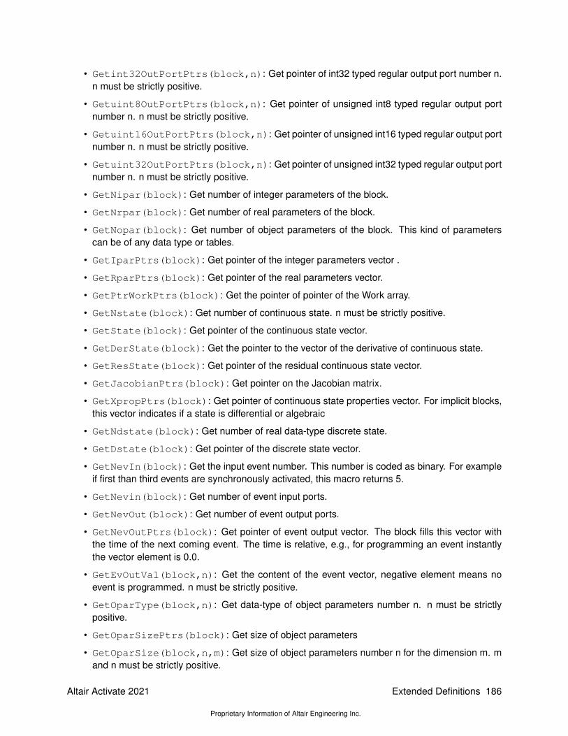
• Getint32OutPortPtrs(block,n): Get pointer of int32 typed regular output port number n.n must be strictly positive.
• Getuint8OutPortPtrs(block,n): Get pointer of unsigned int8 typed regular output portnumber n. n must be strictly positive.
• Getuint16OutPortPtrs(block,n): Get pointer of unsigned int16 typed regular output portnumber n. n must be strictly positive.
• Getuint32OutPortPtrs(block,n): Get pointer of unsigned int32 typed regular output portnumber n. n must be strictly positive.
• GetNipar(block): Get number of integer parameters of the block.
• GetNrpar(block): Get number of real parameters of the block.
• GetNopar(block): Get number of object parameters of the block. This kind of parameterscan be of any data type or tables.
• GetIparPtrs(block): Get pointer of the integer parameters vector .
• GetRparPtrs(block): Get pointer of the real parameters vector.
• GetPtrWorkPtrs(block): Get the pointer of pointer of the Work array.
• GetNstate(block): Get number of continuous state. n must be strictly positive.
• GetState(block): Get pointer of the continuous state vector.
• GetDerState(block): Get the pointer to the vector of the derivative of continuous state.
• GetResState(block): Get pointer of the residual continuous state vector.
• GetJacobianPtrs(block): Get pointer on the Jacobian matrix.
• GetXpropPtrs(block): Get pointer of continuous state properties vector. For implicit blocks,this vector indicates if a state is differential or algebraic
• GetNdstate(block): Get number of real data-type discrete state.
• GetDstate(block): Get pointer of the discrete state vector.
• GetNevIn(block): Get the input event number. This number is coded as binary. For exampleif first than third events are synchronously activated, this macro returns 5.
• GetNevin(block): Get number of event input ports.
• GetNevOut(block): Get number of event output ports.
• GetNevOutPtrs(block): Get pointer of event output vector. The block fills this vector withthe time of the next coming event. The time is relative, e.g., for programming an event instantlythe vector element is 0.0.
• GetEvOutVal(block,n): Get the content of the event vector, negative element means noevent is programmed. n must be strictly positive.
• GetOparType(block,n): Get data-type of object parameters number n. n must be strictlypositive.
• GetOparSizePtrs(block): Get size of object parameters
• GetOparSize(block,n,m): Get size of object parameters number n for the dimension m. mand n must be strictly positive.
Altair Activate 2021
Proprietary Information of Altair Engineering Inc.
Extended Definitions 186

• GetOparSize (block,n,1): Get first dimension (row size) of object parameters number n .n must be strictly positive.
• GetOparSize (block,n,2): Get second dimension (column size) of object parametersnumber n . n must be strictly positive.
• GetOparPtrs(block,n): Get pointer of object parameters number n.
• GetRealOparPtrs(block,n): Get pointer of real object parameters number n.
• GetImagOparPtrs(block,n): Get pointer of imaginary part of object parameters number n.
• Getint8OparPtrs(block,n): Get pointer of int8 typed object parameters number n.
• Getint16OparPtrs(block,n): Get pointer of int16 typed object parameters number n.
• Getint32OparPtrs(block,n): Get pointer of int32 typed object parameters number n.
• Getuint8OparPtrs(block,n): Get pointer of unsigned int8 typed object parameters num-ber n.
• Getuint16OparPtrs(block,n): Get pointer of unsigned int16 typed object parametersnumber n.
• Getuint32OparPtrs(block,n): Get pointer of unsigned int32 typed object parametersnumber n.
• GetStringOparPtrs(block,n): Get pointer of unsigned int32 typed object parametersnumber n.
• GetNoz(block): Get number of object discrete state.
• GetOzType(block,n): Get type of object discrete state number n.
• GetOzTypePtrs(block): Get type of object state.
• GetOzSizePtrs(block): Get size of object state.
• GetOz(block): Get object state
• GetOzSize(block,n,m): Get size of object state number n for the dimension m.
• GetOzSize (block,n,1): Get first dimension (row size) of object state number n.
• GetOzSize (block,n,2): Get second dimension (column size) of object state number n.
• GetOzPtrs(block,n): Get pointer of object state number n.
• GetRealOzPtrs(block,n): Get pointer of real object state number n.
• GetImagOzPtrs(block,n): Get pointer of imaginary part of object state number n.
• Getint8OzPtrs(block,n): Get pointer of int8 typed object state number n.
• Getint16OzPtrs(block,n): Get pointer of int16 typed object state number n.
• Getint32OzPtrs(block,n): Get pointer of int32 typed object state number n.
• Getuint8OzPtrs(block,n): Get pointer of unsigned int8 typed object state number n.
• Getuint16OzPtrs(block,n): Get pointer of unsigned int16 typed object state number n.
• Getuint32OzPtrs(block,n): Get pointer of unsigned int32 typed object state number n.
187 Extended Definitions
Proprietary Information of Altair Engineering Inc.
Altair Activate 2021

• GetSizeOfOz(block,n): Get the data size of each element of the block discrete OZ state.As an example, if the data type of OZ is Double, this macro returns sizeof(Double).
• GetSizeOfOpar(block,n): Get the data size of each element of the block Opar parameter.As an example, if the data type is Double, this macro returns sizeof(Double).
• GetSizeOfOut(block,n): Get the sizeof of the regular output port number n. Get the datasize of each element of the block output. As an example, if the data type is Double, this macroreturns sizeof(Double).
• GetSizeOfIn(block,n): Get the data size of each element of the block input. As an exam-ple, if the data type is Double, this macro returns sizeof(Double).
• GetNg(block): Get number of zero crossing surface.
• GetGPtrs(block): Get pointer of the zero crossing vector. This vector should be filled by theblock and contain the zero-crossing surfaces.
• GetJrootPtrs(block): Get pointer of the direction of the zero crossing vector
• GetNmode(block): Get number of modes
• GetWorkPtrs(block): Get the pointer of the Work array.
• GetModePtrs(block): Get pointer of the mode vector
• GetLabelPtrs(block): Get pointer of the block label
• GetBoolInPortPtrs(block,n): Get pointer of boolean typed regular input port number n.
• GetBoolOutPortPtrs(block,n): Get pointer of boolean typed regular output port numbern.
• GetImplicitFlag(block): check if the block is implicit (DAE)
• GetBlockType(block): Get Block Type.
• GetBlockNamePtrs(block): Get Block Name structure pointer ( II)
• GetBlockName(block): Get the block instance name
• GetBlockNSubNames(block): list of block inside a virtual block
• GetBlockSubName(block,n): Get the block number n from the list of blocks inside a virtualblock
• GetDept(block): check if a block is time dependent
• GetInher(block): Get the inheritance method, 0)no inheritance 1)inheritance from a singleevent input 2)inheritance from multiple event inputs
• GetAjac(block): check if the block provides the Analytical Jacobian
• GetCorrPtr(block): Get pointer of projection corrector vector
• GetConstraintKind(block): This macro returns the constraint type defined by the block.There are two constraint types can be defined by the block:
– CONSTRAINT: Additional equations defining algebraic equation between states are addedto the block dynamical equations. In this case number of additional equations should begiven by macro SetNConstraint(block,n).
Altair Activate 2021
Proprietary Information of Altair Engineering Inc.
Extended Definitions 188
– PROJECTION: When this option is chosen, states values are readjusted to meet someconstraints inside the model.
• GetNConstraint(block): Get number of Constraints, if the constraint type is CONSTRAINT
• SetAjac(block): Indicate that the block provides the Analytical Jacobian
9.1.4 Macros for accessing the simulator structure
The followign macros used to access some global variables or information such as simulator currenttime or error tolerances. These variables are available on the simulator structure.
• GetFinalTime(block): Get the final time of the simulation.
• GetHmax(block): Get the (maximum) step-size provided by the user (Note that this value canbe auto). If the solver is fixed-step, this value will be the step-size of the solver.
• GetHmaxUsed(block): Get the (maximum) step-size actually used by the simulator.
• GetAtol(block): Get the absolute error tolerance used by the simulator.
• GetRtol(block): Get the relative error tolerance used by the simulator.
• GetVssInitialTime(block): Get the start time of the simulation used by the simulator.
• GetTtol(block): Get the error tolerance in time provided by the user (Note that this valuecan be auto).
• GetTtolUsed(block): Get the error tolerance in time actually used by the simulator.
• GetAtolptr(block): Get the absolute error tolerance vector used by the simulator.
• GetBlockNum(block): Get the ordering number of the block defined by the simulator.
• GetSQRU(block): Get the square-root of the machine epsilon used by the simulator.
• GetNeq(block): Get the number of continuous-time state of the model used by the simulator.
• GetNzero(block): Get the number of zero-crossing surfaces of the model used by the simu-lator.
• GetInitialX(block): Get initial value of continuous-time states of the model used by thesimulator.
• GetInitialXd(block): Get initial value of the derivative of continuous-time states of themodel used by the simulator.
• IsHotReStart(block): Indicates if the block is called while the solver is just being reinitial-ized after a discrete event. 0 means that the solver is just being restarted.
• isColdRestart(block): Same as IsHotReStart, but 1 means that the solver is just beingrestarted.
• DoColdRestart(block): Force the solver to reinitialize.
• GetVssTime(block): Get the current time in the simulator.
• GetSimulationPhase(block): Get the phase of the simulation used by the simulator.
• GetMeshPoint(block): Get the last mesh-point time instant taken by the solver.
189 Extended Definitions
Proprietary Information of Altair Engineering Inc.
Altair Activate 2021

• GetLastStepSize(block): Get the last step-size successfully taken by the solver.
• GetNextTryStepSize(block): Get the next step-size being tried by the solver.
• GetSimulatorInitiated(block): indicates if the simulator has finished the initializationof the model.
• isStopRequested(block): Indicates if the user has pressed the stop button to terminatethe simulation.
• StopSimulation(block,val): Force the simulator to finish the simulation.
• isZeroCrossingEnabled(block): Indicates if the zero-crossing option is enabled in thesimulator.
• isModeEnabled(block): Indicates if handling mode is enabled by the simulator.
• GetXpropPtr(block): Get the vector of the xproperty assigned to the block by the simulator.This vector is used to define if a continuous-state is differential or algebraic.
• GetAlphaPt(block): Get the actual value of alpha (α) when computing the Jacobian. Notethat the Jacobian of the DAe 0 = F (x, x) is computed as follows: J = α∂F (x,x)
∂x + β ∂F (x,x)∂x .
• GetBetaPt(block): Get the actual value of beta (β) when computing the Jacobian.
• isinTryPhase(block): Indicates if the block is being called by the numerical solver. In thiscase, the value given to the block is not a definitive value.
• areModesFixed(block): Indicates that if the block is being called with mode values fixed orrelaxed (can be changed/updated by the block).
• isZeroCrossing(block): Indicates if the block is being called at a zero-crossing event.
• isDiscreteEvent(block): Indicates if the block is being called at a discrete event.
• isMeshPoint(block): Indicates if the block is being called at a mesh-point.
• isDiscreteLeftLimit(block): Indicates if the block is being called at a left-limit of a dis-crete event.
• isZeroCrossingLeftLimit(block): Indicates if the block is being called at a left-limit ofa zero-crossing event.
• isExitInitialization(block): Indicates if the block is being called at the end of theinitialization.
• isSimulatorInInitializationPhase(block): Indicates if the simulator is still in theinitialization stage.
• isSimulatorInTerminationPhase(block): Indicates if the simulator is in the termina-tion stage.
• Coserror(block,msg,âAe): Emits an error message. This message usually follows an errorin the block and is followed by a return from the block.
• Coswarning(block,msg,âAe): Emits a warning message.
• Cosmessage(block,msg,âAe): Emits a purely informative message.
• GetSimulatedModelName(block): returns the name of the model being simulated.
• GetSimulatedModelFilePath(block): returns the path of the model being simulated.
Altair Activate 2021
Proprietary Information of Altair Engineering Inc.
Extended Definitions 190

• GetSimulatedModelTempDir(block): returns the path of the temporary folder for the cur-rent model.
• isInDebugMode(block): Indicates if the simulation is done in the debug mode.
• Discard(block): This The block can indicate the numerical solver that the state derivativecannot be computed and the solver should take smaller step size. This feature is used in flag=VssFlag_Derivatives, for ther situation is treated as error.
• isinRepeatEventBlock(block): Indicates if this call to the block is the repetition of aprevious event.
9.2 Block builder
The construction of simulation functions has been presented in the previous section. A C simula-tion function can be associated with a CCustomBlock and be used in Activate models. The CCus-tomBlock however has a generic user interface in the BDE which cannot be customized. The cus-tomization can be done by hiding this block inside a masked Super Block, however the level of cus-tomization is limited. A new basic block provides a much higher level of customization, as it will be seenin the next section.
Basic blocks and programmable super blocks can be constructed using the Block builder tool. Thesetwo types of blocks are similar at the BDE level and so is their construction. The block must provide itsgraphical and strcutural properties: parameters, numbers of ports of different types, block size, color,icon, etc., in an XML file. It must also provide in the case of the basic block: the list of simulationfunctions used by the block and three OML functions instantiating the block. In the case of the pro-grammable super block, only one OML function is required.
By using the Block builder, user needs not worry about creating XML files or even defining OML func-tions. He/she needs simply provide the required information and the block builder creates the XML file.For the OML functions, only part of the code must be provided, the rest is auto-generated by the Blockbuilder.
The Block builder interface contains 7 tabs:
1. Label: used to define the block default name, its location and whether or not it is visible by default.
2. Atom: used to define the internal properties of the block. Its definition depends on whether theblock is a basic block or a prgorammable super block. Both cases will be discussed in detailslater.
3. Properties: used for documenting the block.
4. Parameters: used to define the number, type, name and default values of the block parameters.Callback functions can also be associated with parameters.
5. Graphics: used to set the block shape, size and color.
6. Ports: used to define the number of ports, their types and locations.
7. Icon: used to associate an image to the block icon. A second image may be used when the blockis mirrored.
The block builder can be invoked from scratch or by selecting, in the current diagram, a basic blockor a masked Super Block. In the latter case, the properties of the selected block are reflected in the
191 Extended Definitions
Proprietary Information of Altair Engineering Inc.
Altair Activate 2021

Block builder interface so that if no modifications are done, the block builder creates a duplicate ofthe selected block (in the case the selected block is a masked Super Block, the new block will bean equivalent programmable super block). The ability to initialize the Block builder interface using anexisting block is very helpful for defining new blocks: user can start with an existing block similar to thenew block and edit only the differences.
Atom is where the internal structure of the block is defined. The content of all the tabs, except Atom,are straightforwad to understand and edit, and are identical for both basic blocks and programmablesuper blocks.
9.2.1 Atom: Basic block
For a basic block, Atom provides the list of simuation functions. In general a block has more than onesimulation function, in particular if it supports different data types. For each simulation function, theshared library and the corresponding entry point is specified. A basic block definition requires up to 3OML functions. The partial code for these functions are provided in Atom.
The first function, SetParameters, is the main function; it creates the block structure based on blockparameters and port properties. The other two functions are used to modify this structure if needed. TheOML code that must be provided to define the SetParameters function assumes that the followingsare availble:
• the name of the block, defined in the variable _label,
• the block parameter values under the name of the corresponding parameters,
• the diagram where the block is to be placed, defined in the variable _diagram.
For a basic block, the block added to diagram is of type “block”, so the OML code invariably containsthe following lines
_block = vssAddNewObject (’Block’, _diagram);vssSetBlockName (_block, _label);
The structure _block is then supplemented using provided APIs. For example simulation parametersopar are defined based on the value of block parameters. The code used here vary considerablydepending on the properties of the new block. Instead of providing an exhaustive list of APIs and theirusage, we encourage users to examine the codes associated with existing blocks, in particular blockshaving similar properties to that of the new block. By doing so, the creation of the new code is reducedto changing a few lines of an existing code.
The SetParameters function is automatically created based on the user provided OML code mainlyby adding systematic tests so that in case of error, an informative error message can be generated.This function is called in the model evaluation phase, which constructs the model structure used forcompilation and simulation.
The two other functions are used to set the values not set by the SetParameters function in the blockstructure. The non-set values correspond to undefined size and data types of block input and ouputports. The SetParameters function in general specifies all the properties of the block structure butit can leave out some porperties, to be found by the compiler. In particular the size of an input maybe left unknown. This is done by setting the size vector to negative values, [−1,−2]. This means theinput has totally arbitrary size. If another input or an output size is also set to [−1,−2], then the lattersize is also arbitray but equal to the former. If an input size is set to [−1,−1], then the matrix is a
Altair Activate 2021
Proprietary Information of Altair Engineering Inc.
Extended Definitions 192

square matrix of arbitrary size. Negative value means unknown, but the same negative values meansame sizes. This way constraints on block port sizes can be imposed for many common blocks. Forexample the matrix transpose block has input size [−1,−2] and output size [−2,−1]. This captures allthe constraints imposed by the block on its input and output.
The compiler figures out the actual port sizes by taking into account these constraints and the waythe blocks are interconnected. Similarly block port data types may be set to arbitrary and the compilerdeduces the actual types. Once the compiler completes the computation of block input/output datasizes and types, the block OML function Reset is called with argument the block structure includingthe actual port data sizes and types. This function can then modify other block properties if needed.In most cases, the block Reset function selects the appropriate simulation function based on the portdata types. The Reset function is defined in Atom based on user-supplied code.
The last OML function associated with a basic block is SetIO. This function is defined when theconstraints on port data types and sizes cannot be imposed by using negative numbers. For examplea block may be such that the size of its input is arbitrary and the size of its output is one bigger thanthe size of its input. These “exotic” constraints cannot be imposed using negative size values. In suchcases the block can provide a SetIO function working on the block structure (constructed previously bySetParameters. This function, based on current status of port sizes and types, may replace negativeport sizes and types by positive values. This function may be called many times during compilation. Forthe example where the output is one bigger than the input, the function can fully define the port sizes ifeither the input or the output size is known, when the function SetIO is called.
Most user defined blocks don’t require SetIO and Reset functions and the associated code in Atomshould be left empty.
9.2.2 Atom: Programmable Super Block
For programmable super blocks, there is no simulation function to define and there is only the SetParametersfunction that needs to be defined in Atom. In this case the content being defined is a “subsystem” andthe OML code is used to construct the diagram inside the block. The code contains:
_block = vssAddNewObject(’SubSystem’,_diagram);_diagr= vssCreateObject(’Diagram’);
and then goes on populating _diagr with blocks and links constructing a diagram.
The definition of a block inside the diagram is done by defining the block parameters by an OMLstruct,loading the block from the corresponding library and instantiating it. Consider for example the blockDiscreteDelay, which has parameters init_cond, typ, and externalActivation. This blockcan be instantiated in the diagram _diagr for example as follows_params=struct();_params.init_cond=z0;_params.typ=’double’;_params.externalActivation=0;vssLoadBlock(’system’,’Dynamical’,’DiscreteDelay’);_vss._palettes.(’_system’).(’Dynamical’).(’DiscreteDelay’).setparams(_diagr,’DiscreteDelay’,_params);
Here the initial condition is set to z0, which must be a parameter of the programmable super block.
Links are created using the OML function vssAdd_Link. The following instruction for example con-nects the first ouptut of the Input block to the first output of the DiscreteDelay block by a regular link:
vssAdd_Link(_diagram,’Input’,’DiscreteDelay’,1,1,0,1,1);
193 Extended Definitions
Proprietary Information of Altair Engineering Inc.
Altair Activate 2021

When the Block builder is invoked with a masked Super Block, the SetParameters function of theblock is generated automatically containing the code that constructs the diagram inside the Super Block.In this case the diagram is fixed.
A fixed-diagram programmable super blocks is not particularly useful because it can also be imple-mented by a standard masked Super Block. It can however be a good starting point for defining theSetParameters function of a general programmable super block where the diagram inside and thenumber of ports can depend on block parameters. This process is illustrated through the followingexample.
Example
Here the problem is to create a shift register block where each register value is exposed through aseparate output. The number of registers (and outputs) is thus variable, equal to nout, given as ablock parameter. In case of three registers/outputs (nout=3), the diagram is simple:
This Super Block will be used as a starting point for the constrcution of the programmable super block.
First, the Super Block is prepared to be masked by defining the undefined variables z0 and nout inthe Initialization script of the model. Auto-masking can then be applied:
Altair Activate 2021
Proprietary Information of Altair Engineering Inc.
Extended Definitions 194

which yields:
Now that the Super Block is masked, block builder can be applied to create a new block. The Blockbuilder now contains a good starting point for defining the new block.
Some of the properties must be modified for the new block. In particular the number of ports in thePorts tab. Originally the ports are fixed:
195 Extended Definitions
Proprietary Information of Altair Engineering Inc.
Altair Activate 2021

The Ports tab must be edited to allow the number of outputs to be variable, in particular nout:
The Parameters tab must be edited to change the property of the parameter nout to make it of type“Number”. Structural properties such as the number of ports can only be set by parameters of type“Number”.
Altair Activate 2021
Proprietary Information of Altair Engineering Inc.
Extended Definitions 196

The main modification to be made is of course in the SetParameters code (inside the Atom tab)which defines the diagram inside the Super Block. The current code constructs the diagram by instan-tiating blocks and connecting them for the case nout=3. Note that no graphical properties are usedat this point: the diagram does not have a corresponding graphics. The code gnerated by the Blockbuilder for the fixed diagram is as follows:function _setdiagram_1 (_diagram, _label, __fenv__)_curdiagram=_diagram;_curlabel=_label;importenv(__fenv__);_diagram=_curdiagram;_label=_curlabel;clear _curdiagram;clear _curlabel;global _vss;global __OBJ_ERR_;_parent = __OBJ_ERR_.(’block’);__OBJ_ERR_.(’type’)=’context’;if isscalar(z0) z0=z0*ones(nout,1);end__OBJ_ERR_.(’block’)=vssConstructBlockFullName(_parent,’Output_2’);__OBJ_ERR_.(’type’)=’parameters’;_params=struct();_params.portNumber=3;_params.insize=[-1;-2];_params.intyp=’inherit’;vssLoadBlock(’system’,’Ports’,’Output’);_vss._palettes.(’_system’).(’Ports’).(’Output’).setparams(_diagram,’Output_2’,_params);__OBJ_ERR_.(’block’)=vssConstructBlockFullName(_parent,’DiscreteDelay_2’);__OBJ_ERR_.(’type’)=’parameters’;_params=struct();_params.init_cond=z0(3);_params.typ=’double’;_params.externalActivation=0;vssLoadBlock(’system’,’Dynamical’,’DiscreteDelay’);_vss._palettes.(’_system’).(’Dynamical’).(’DiscreteDelay’).setparams(_diagram,’DiscreteDelay_2’,_params);__OBJ_ERR_.(’block’)=vssConstructBlockFullName(_parent,’Output_1’);__OBJ_ERR_.(’type’)=’parameters’;
197 Extended Definitions
Proprietary Information of Altair Engineering Inc.
Altair Activate 2021

_params=struct();_params.portNumber=2;_params.insize=[-1;-2];_params.intyp=’inherit’;vssLoadBlock(’system’,’Ports’,’Output’);_vss._palettes.(’_system’).(’Ports’).(’Output’).setparams(_diagram,’Output_1’,_params);__OBJ_ERR_.(’block’)=vssConstructBlockFullName(_parent,’Output’);__OBJ_ERR_.(’type’)=’parameters’;_params=struct();_params.portNumber=1;_params.insize=[-1;-2];_params.intyp=’inherit’;vssLoadBlock(’system’,’Ports’,’Output’);_vss._palettes.(’_system’).(’Ports’).(’Output’).setparams(_diagram,’Output’,_params);__OBJ_ERR_.(’block’)=vssConstructBlockFullName(_parent,’Input’);__OBJ_ERR_.(’type’)=’parameters’;_params=struct();_params.portNumber=1;_params.outsize=[-1;-2];_params.outtyp=’inherit’;_params.dept=0;vssLoadBlock(’system’,’Ports’,’Input’);_vss._palettes.(’_system’).(’Ports’).(’Input’).setparams(_diagram,’Input’,_params);__OBJ_ERR_.(’block’)=vssConstructBlockFullName(_parent,’Block’);__OBJ_ERR_.(’type’)=’parameters’;_params=struct();vssLoadBlock(’system’,’Links’,’Split’);_vss._palettes.(’_system’).(’Links’).(’Split’).setparams(_diagram,’Block’,_params);__OBJ_ERR_.(’block’)=vssConstructBlockFullName(_parent,’DiscreteDelay_1’);__OBJ_ERR_.(’type’)=’parameters’;_params=struct();_params.init_cond=z0(2);_params.typ=’double’;_params.externalActivation=0;vssLoadBlock(’system’,’Dynamical’,’DiscreteDelay’);_vss._palettes.(’_system’).(’Dynamical’).(’DiscreteDelay’).setparams(_diagram,’DiscreteDelay_1’,_params);__OBJ_ERR_.(’block’)=vssConstructBlockFullName(_parent,’Split’);__OBJ_ERR_.(’type’)=’parameters’;_params=struct();vssLoadBlock(’system’,’Links’,’Split’);_vss._palettes.(’_system’).(’Links’).(’Split’).setparams(_diagram,’Split’,_params);__OBJ_ERR_.(’block’)=vssConstructBlockFullName(_parent,’DiscreteDelay’);__OBJ_ERR_.(’type’)=’parameters’;_params=struct();_params.init_cond=z0(1);_params.typ=’double’;_params.externalActivation=0;vssLoadBlock(’system’,’Dynamical’,’DiscreteDelay’);_vss._palettes.(’_system’).(’Dynamical’).(’DiscreteDelay’).setparams(_diagram,’DiscreteDelay’,_params);vssAdd_Link(_diagram,’Output_2’,’DiscreteDelay_2’,1,1,1,0,1);vssAdd_Link(_diagram,’DiscreteDelay_1’,’Block’,1,1,0,1,1);vssAdd_Link(_diagram,’Block’,’Output_1’,1,1,0,1,1);vssAdd_Link(_diagram,’DiscreteDelay_2’,’Block’,1,2,1,0,1);vssAdd_Link(_diagram,’Input’,’DiscreteDelay’,1,1,0,1,1);vssAdd_Link(_diagram,’DiscreteDelay’,’Split’,1,1,0,1,1);vssAdd_Link(_diagram,’Split’,’DiscreteDelay_1’,1,1,0,1,1);vssAdd_Link(_diagram,’Split’,’Output’,2,1,0,1,1);end_block = vssAddNewObject(’SubSystem’,_diagram);_diagr= vssCreateObject(’Diagram’);_setdiagram_1(_diagr,_label,getcurrentenv());vssSet_SubSystem(_block,1,3,0,0,0,_label,_diagr);
The variable __OBJ_ERR_ is used to anchor the error locations for generating precise error messages.In the case of programmable super blocks, this is in general not very useful and it is better to referenceall error message to the parent block (the programmable super block). User in general does not knowabout the content of this block.
Altair Activate 2021
Proprietary Information of Altair Engineering Inc.
Extended Definitions 198

The above code, which corresponds to the fixed diagram with three delays and outputs, is extended sothat it can work for arbitrary nout number of delays and outputs. Note that the individual error tags areremoved so that all errors are referred to the parent. The script used in the context of the Super Blockis also extended to produce better error messages:function shiftreg_setdiagram_1 (_diagram, _label, __fenv__)_curdiagram=_diagram;_curlabel=_label;importenv(__fenv__);_diagram=_curdiagram;_label=_curlabel;clear _curdiagram;clear _curlabel;global _vss;global __OBJ_ERR_;_parent = __OBJ_ERR_.(’block’);__OBJ_ERR_.(’type’)=’context’;if isscalar(z0) z0=z0*ones(nout,1); elseif length(z0)~=nout error(’size of z0 must match nb of outputs.’);end__OBJ_ERR_.(’block’)=vssConstructBlockFullName(_parent,’DiscreteDelay’);_params=struct();_params.init_cond=z0(1);_params.typ=’double’;_params.externalActivation=0;vssLoadBlock(’system’,’Dynamical’,’DiscreteDelay’);_vss._palettes.(’_system’).(’Dynamical’).(’DiscreteDelay’).setparams(_diagram,’DiscreteDelay’,_params);_params=struct();vssLoadBlock(’system’,’Links’,’Split’);_vss._palettes.(’_system’).(’Links’).(’Split’).setparams(_diagram,’Split_1’,_params);_params=struct();_params.portNumber=1;_params.outsize=[-1;-2];_params.outtyp=’inherit’;_params.dept=0;vssLoadBlock(’system’,’Ports’,’Input’);_vss._palettes.(’_system’).(’Ports’).(’Input’).setparams(_diagram,’Input’,_params);_params=struct();_params.portNumber=1;_params.insize=[-1;-2];_params.intyp=’inherit’;vssLoadBlock(’system’,’Ports’,’Output’);_vss._palettes.(’_system’).(’Ports’).(’Output’).setparams(_diagram,’Output’,_params);vssAdd_Link(_diagram,’Input’,’DiscreteDelay’,1,1,0,1,1);vssAdd_Link(_diagram,’DiscreteDelay’,’Split_1’,1,1,0,1,1);vssAdd_Link(_diagram,’Split_1’,’Output’,2,1,0,1,1);for i=2:nout-1
_params=struct();_params.init_cond=z0(i);_params.typ=’double’;_params.externalActivation=0;vssLoadBlock(’system’,’Dynamical’,’DiscreteDelay’);_vss._palettes.(’_system’).(’Dynamical’).(’DiscreteDelay’).setparams(_diagram,[’DiscreteDelay_’,...
num2str(i-1)],_params);_params=struct();_params.portNumber=i;_params.insize=[-1;-2];_params.intyp=’inherit’;vssLoadBlock(’system’,’Ports’,’Output’);_vss._palettes.(’_system’).(’Ports’).(’Output’).setparams(_diagram,[’Output_’,num2str(i-1)],_params);_params=struct();vssLoadBlock(’system’,’Links’,’Split’);_vss._palettes.(’_system’).(’Links’).(’Split’).setparams(_diagram,[’Split_’,num2str(i)],_params);vssAdd_Link(_diagram,[’Split_’,num2str(i-1)],[’DiscreteDelay_’,num2str(i-1)],1,1,0,1,1);vssAdd_Link(_diagram,[’DiscreteDelay_’,num2str(i-1)],[’Split_’,num2str(i)],1,1,0,1,1);vssAdd_Link(_diagram,[’Split_’,num2str(i)],[’Output_’,num2str(i-1)],2,1,0,1,1);
end_params=struct();_params.init_cond=z0(nout);_params.typ=’double’;
199 Extended Definitions
Proprietary Information of Altair Engineering Inc.
Altair Activate 2021

_params.externalActivation=0;vssLoadBlock(’system’,’Dynamical’,’DiscreteDelay’);_vss._palettes.(’_system’).(’Dynamical’).(’DiscreteDelay’).setparams(_diagram,[’DiscreteDelay_’,...
num2str(nout-1)],_params);_params=struct();_params.portNumber=nout;_params.insize=[-1;-2];_params.intyp=’inherit’;vssLoadBlock(’system’,’Ports’,’Output’);_vss._palettes.(’_system’).(’Ports’).(’Output’).setparams(_diagram,[’Output_’,num2str(nout-1)],_params);vssAdd_Link(_diagram,[’DiscreteDelay_’,num2str(nout-1)],[’Output_’,num2str(nout-1)],1,1,0,1,1);vssAdd_Link(_diagram,[’Split_’,num2str(nout-1)],[’DiscreteDelay_’,num2str(nout-1)],1,1,0,1,1);end_block = vssAddNewObject(’SubSystem’,_diagram);_diagr= vssCreateObject(’Diagram’);shiftreg_setdiagram_1(_diagr,_label,getcurrentenv());vssSet_SubSystem(_block,1,nout,0,0,0,_label,_diagr);
The new repeated blocks are named by extensions _2, _3, up to nout. This is not needed for linkswhich are not named.
After creating the first layer of blocks, the repeated structure is created within the following for loop:
for i=2:nout-1....
end
The final layer is created after the for loop. Another change needs to be made in the code to changethe number of outputs of the new block:
vssSet_SubSystem(_block,1,3,0,0,0,_label,_diagr);
is replaced by
vssSet_SubSystem(_block,1,nout,0,0,0,_label,_diagr);
indicating that the block has nout outputs and not 3.
The newly created block can be moved to a new model and its parameters can be set to desired values:
and tested:
Altair Activate 2021
Proprietary Information of Altair Engineering Inc.
Extended Definitions 200
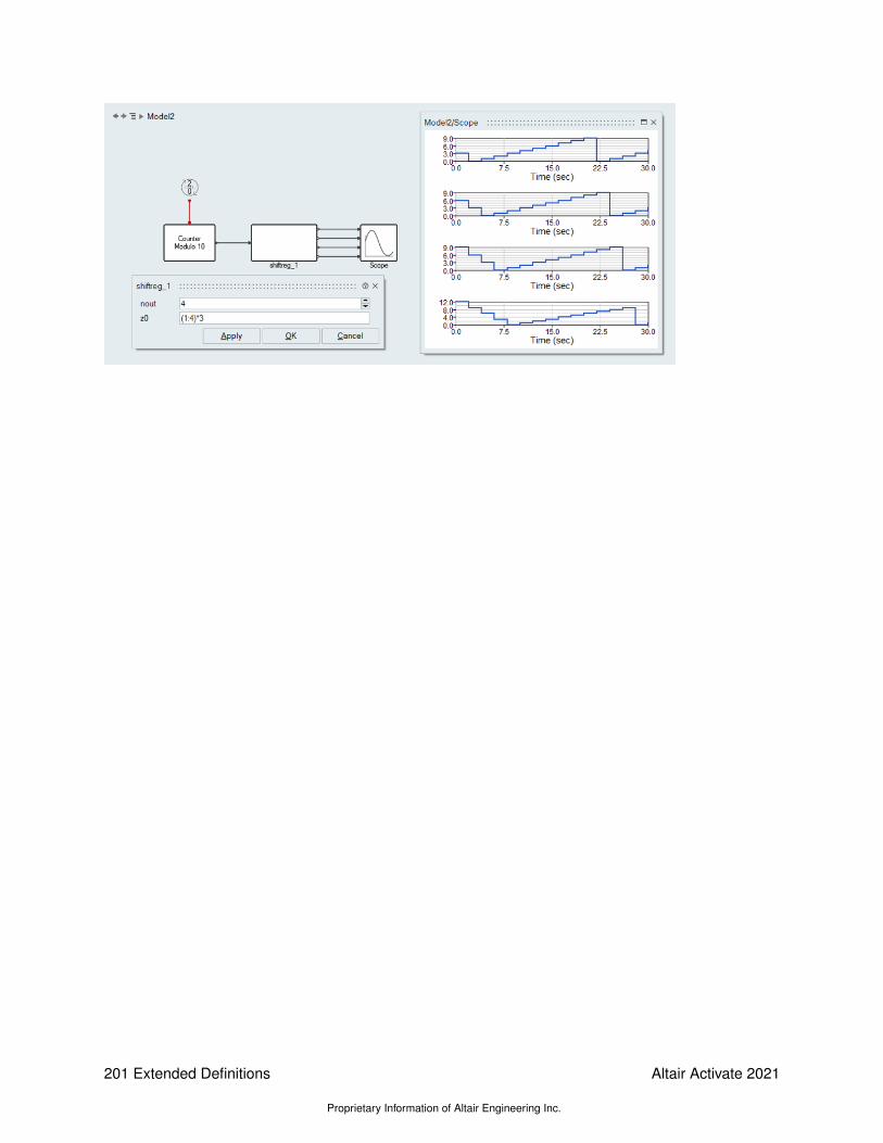
201 Extended Definitions
Proprietary Information of Altair Engineering Inc.
Altair Activate 2021

Altair Activate 2021
Proprietary Information of Altair Engineering Inc.
Extended Definitions 202

Chapter 10
Activate hybrid simulator and its interfacewith numerical solvers
Activate is a simulator for hybrid systems. A hybrid system is composed of discrete-time and continuous-time subsystems in which the values of continuous-time variables are governed by differential equationsand discrete-time variables are updated at time instants called event times. In Activate several numeri-cal solvers have been interfaced with the simulator to integrate the differential equations. These numer-ical solvers have many control parameters that should be used to optimize the simulation in differentsituations. Indeed, in the hybrid context, controlling the solver, which should be done automaticallyand should remain transparent to the user, is a complex matter due to the interactions between thecontinuous-time dynamics and the rest of the system. In this document, the simulator of Activate, thenumerical solvers and the interface between the simulator and the numerical solvers will be discussed.
10.1 Introduction
A hybrid system is a dynamical system that involves the interactions of continuous states and discretestates. As an example, consider a bouncing ball which is a hybrid system since the state variables(position and speed) vary continuously according to Newton laws when falling, but they have a discretechange (speed is reversed) when entering in collision with the ground. Jump in state and discontinu-ities are basic phenomena that cannot be represented and analyzed by methods elaborated either incontinuous-time or in discrete-time system theory. In a hybrid system composed of continuous-time anddiscrete-time subsystems, each subsystem can interact with the other, e.g., if a discrete-time variableused in a differential equation is changed all the continuous-time variables that depend on this valuemay change. This would imply a discontinuity in these variables.
The discrete-time part of a hybrid system is activated by events and events introduce discontinuitiesin continuous-time variables or in their time derivatives. Events may come from several sources suchas intervention by human operators or from an input control or may be programmed to be generatedautonomously.
There are two event types that are more important. They are events that occur at a given time, i.e., apredictable event (or time events), and those which appear when a variable reaches a certain thresholdvalue, i.e., an unpredictable (or a zero-crossing event).
203 Extended Definitions
Proprietary Information of Altair Engineering Inc.
Altair Activate 2021

The underlying hybrid formalism in Activate allows modeling very general hybrid systems: systemsincluding continuous, discrete-time and event based behaviors. Activate includes a graphical editorfor constructing models by interconnecting blocks, representing predefined or user-defined functions, acompiler, a simulator, and code generation facilities. The graphical editor allows creating and connectingblocks selected from block palettes. A Activate block diagram is composed of blocks and connectionlinks. There are two connection link types; regular and activation links. The regular links representcontinuous-time or discrete-time signals or variables in the model, while the activation links transmitactivation timings information. A block corresponds to an operation and by interconnecting blocksthrough links, a model or an algorithm is constructed. These blocks represent elementary systemsthat can be used as model building blocks. They can have several inputs and outputs, continuous-timestates, discrete-time states, zero-crossing functions, etc. Note that it is not possible to treat an activationlink as a regular link or to interconnect an activation link with a regular link. In order to get an idea whata Activate model looks like, a model of a simple control system implemented in Activate is shown inthe following figure.
Figure 10.1: Simple control model (simple_control1.scm)
In this figure (10.1) the clock block generates a periodic activation signal (events) that activates theScope block. At event times the scope reads its input signal and displays it.
Here is an example of a pure discrete-time system where the state is updated by a periodic clock withperiod T .
x(k + 1) =
x(k) + u(k) if u(k) > 0x(k) otherwise
x(1) = 0
The implementation of this model and its simulation result in Activate are given in following figures(10.2, 10.3). In this model u(k) is generated by a random signal generator block with output valuesbetween [−1,+1].
Altair Activate 2021
Proprietary Information of Altair Engineering Inc.
Extended Definitions 204

Figure 10.2: Discrete model (discretem.scm)
Figure 10.3: Results of Discrete model (discretem.scm)
Now consider the model of the bouncing ball. The model implemented in Activate and its simu-lation result are given in the following figures (10.4, 10.5). In this model when the altitude of theball (x) becomes negative, the zero-crossing block generates an event that resets the LinearContinuous-time block with new state values.
x = vv = −9.8
when (x < 0) then v = −0.9 v
205 Extended Definitions
Proprietary Information of Altair Engineering Inc.
Altair Activate 2021

Figure 10.4: Simple bouncing ball model (simple_bball.scm)
Figure 10.5: Results of Simple bouncing ball model
10.2 Simulation of an hybrid model in Activate
The simulator of Activate is designed to generate the solution of the Activate model, which is veryoften a hybrid system. A hybrid system simulator should be able to perform, discrete-time scheduling,continuous-time integration, and interactions between discrete-time and continuous-time part (zero-crossing events and event handling).
Simulation of a hybrid system is composed of two phases: the discrete-phase and the continuous-phase. In the discrete phase, event scheduling, event activating and state updating (discrete-time andcontinuous-time) is done, and the simulation time does not advance. In the continuous-phase, thenumerical solver integrates the differential equation and the simulation time advances. Integration ofthe continuous-time system is done from one event time to the next event time. The exact time instantof an event may not be known in advance, hence during the continuous-time phase an event detectionprocess is being performed to stop the continuous-phase and enter into the discrete-phase.
The continuous-time parts of a hybrid system can be modeled either by Ordinary Differential Equations
Altair Activate 2021
Proprietary Information of Altair Engineering Inc.
Extended Definitions 206

(ODE), i.e.,
x = f(x, u, t)
y = h(x, u, t)
where x represents the state variable, x denotes the derivative of x with respect to the time variablet, u is the input vector variable, and y defines the output vector, or by Differential Algebraic Equations(DAE)
x1 = f(x1, x2, u, t)
0 = g(x1, x2, u, t)
y = h(x1, x1, x2, u, t)
The first equation is the differential part and the second is the algebraic part of the DAE. This equation isa semi-explicit DAE where differential and algebraic parts can be decomposed. In semi-explicit index-1DAE, the variable whose derivative is present in the equation is referred to as differential equation andothers are called algebraic variables. This equation can be cast in the form
0 = F (x, x, u, t)
y = h(x, x, u, t)
where x = (x1, x2). This system is called a fully implicit DAE. Note that if partial derivative of F withrespect to x is non-singular then it is possible to solve for x in order to obtain an ODE. However, if it issingular, this is no longer possible and the solution must satisfy certain algebraic constraints.
DAEs are characterized by their index. The index of a DAE is the smallest number of differentiationsrequired to obtain an ODE by algebraic manipulations. In general, the higher the index, the greaterthe numerical difficulty one encounters when trying to solve the system numerically. In a semi-explicitindex-1 DAE, variables whose derivatives appear in DAE are called differential variables and the othersare called algebraic.
Modeling a hybrid system very often leads to a differential equation with discontinuities or a multi-mode system such as an automaton (see Documentation of the Automaton block). In simulation ofa hybrid system, state variables or their time derivative may be discontinuous at some time instants.In such a situation special care has to be taken to solve the model by a numerical solver. Somenumerical solvers such as Radau or Lsoda use variable order and variable step-size methods tointegrate. In simulation of a discontinuous model, such solvers may repeat several times the samestep with smaller step-size to obtain a coherent derivative and meet the accuracy requirements at thediscontinuity point. For some problems, the solver may give up with an error message when the stepgets too small, and in other cases the solver may continue with an erroneous result. In general, suchkind of solvers require that the system be sufficiently smooth over an integration period (at least be C0).This means that simulator must make sure to stop and reinitialize the solver at each potential point ofnon-smoothness (discontinuity, discontinuity in the derivative, etc.). The discontinuity handling problemis solved in Activate by introducing the mode variable in Activate.
A multi-mode system is a way of describing non-smooth systems in terms of a finite number of smoothsystems. The idea is to divide the state space of the system into different regions and associate a modeto each region. It is assumed that the system is described in terms of a single smooth model withineach region. A simple example of a multi-mode system, where the model in each mode is described asDAE, is:
0 =
f1(x, x) if g(x) > 0f2(x, x) otherwise
207 Extended Definitions
Proprietary Information of Altair Engineering Inc.
Altair Activate 2021

This system has two modes: the first one is active when g(x) > 0 and the second is when the conditionis not true. The switching between two modes of the system (f1 and f2) may cause discontinuity in thesignals. As a result the system may not be integrated by numerical solvers. Numerical solvers do notlike discontinuities in the differential equation and they assume that the state variables and their firstderivatives are continuous. If the signal is not continuous, special precautions must be taken at thediscontinuity points. To overcome this problem, the discontinuity should be detected and the numericalsolver be reinitialized after the discontinuity point. In order to detect and localize the discontinuity time,the simulator uses zero-crossing functions that cross zero at the discontinuity point. For example, forthe above model, the zero-crossing function to be used by the simulator is g(x). However, to localizethis point, the numerical solver should simulator say f1 and step over the discontinuity point and usethe other model (f2). Using the model beyond the discontinuity point (f2) normally results in repeatedstep failure and a reduction in integration step-size to meet accuracy requirements. For some problemsespecially models with hard discontinuity the solver gives up with an error message when the step getstoo small, and in some other cases the solver may continue with erroneous results. In order to solvethis problem we have associated a mode variable with each zero-crossing function. We use the modevariable to choose a single ODE/DAE when the numerical solver is called. The assigned ODE/DAEdoes not change till the next discontinuity detection or event. For example, for the above model thegeneral solution has been illustrated in the following figure where xa indicates the discontinuity point orthe instant where g(xa) becomes zero.
Before reaching xa, the solver is in (mode=1), i.e. , it uses 0 = f1(x, x) , without considering thef2(x, x) equation even when the solver needs to compute f1(x, x) for g(x) > 0 (the thick dashed line).The solver employs the f1(x, x) equation to integrate until it detects a zero-crossing. Then the solverlocalizes the crossing point and stops just at the discontinuity point (i.e., at x = xa). After detectingthe zero-crossing and stopping the integration, the mode variable should be updated in order to useanother model, i.e., f2(x, x).
In general, when the numerical solver is called, the system of equations should not be changed or showdiscontinuity. During integration, the zero-crossing functions are monitored by the simulator. In caseof any sign change in the zero-crossing functions, the mode variables should be updated to provideanother ODE/DAE to the solver. In Activate, a mode variable is assigned systematically to each zero-crossing function, characterized by If-then-Else conditions, e.g., to simulate the above system,Activate considers the model in the form:
Altair Activate 2021
Proprietary Information of Altair Engineering Inc.
Extended Definitions 208

0 =
f1(x, x) if mode = 1
f2(x, x) if mode = 2
where mode variables are updated at event time instants, with the following rules.
when (g(x) > 0) is true then mode = 1
otherwise mode = 2
It should be mentioned that any If-then-Else condition, not resulting in a discontinuity, can be usedwithout mode variables. For instance, in this system the mode variable is not necessary.
0 =
x2 + x+ 1 if x ≥ 12x2 − x+ 2 otherwise
Using mode variables eliminates solver difficulties over discontinuities but there is still the problem ofinitialization the modes for DAE.
Most of the problems in simulation of hybrid systems are common to both ODE and DAE solvers.However, there is an additional difficulty with the DAE case: the problem of (re)initialization and findingconsistent initial conditions. Simulation of an ODE can be started from any initial state, but simulation ofa DAE should be started from a consistent initial state. A DAE should be initialized with consistent initialvalues to be solved by a numerical solver, i.e., initial values of states and their derivatives needs to beconsistent with the DAE and some other hidden equations resulted from differentiation of the DAE.
Computation of consistent initial conditions is not in general an easy problem and it becomes particularlydifficult for multi-mode DAE (defined with several modes). The search for the initial condition in this caseis not just the classical problem of finding zeros of smooth functions but it is interlaced with searchingfor the correct mode value. Indeed, each mode value implies a smooth function and the solution of thisfunction may imply another mode value.
The classification in terms of differential and algebraic is also a key element in the study of multi-model DAEs, and in particular, the problem of finding consistent initial conditions since the classificationspecifies which variables are solved for. Consider, for example, the following multi-model DAE
x = sin(t) sin(x)if (x < 1) then y = 2 else y = 3
where in Activate, it is rewritten as:
DAE :
x = sin(t) sin(x)if (Mode1 = 1) then y = 2 else y = 3
Mode changing :
when (x < 1) then Mode1 = 1when (x ≥ 1) then Mode1 = 2
In this example, x is a differential variable and its initial value is given. On the other hand, y is analgebraic variable. This multi-model DAE is well-posed and it is easy to find consistent initial conditionsfor it. In this case, the condition that needs to be tested involve the variable x which is given. Nowconsider the following multi-model DAE
x = x+ y + zif (y < 1) then z = 0, else z = 3if (z < 1) then y = 0, else y = 3
209 Extended Definitions
Proprietary Information of Altair Engineering Inc.
Altair Activate 2021

where in Activate, we use:
ODE :
x = x+ y + zif ( Mode1 = 1 ) then z = 0, else z = 3if ( Mode2 = 1 ) then y = 0, else y = 3
Zero-crossing :
when (y < 1) then Mode1 = 1
when (y ≥ 1) then Mode1 = 2
when (z < 1) then Mode2 = 1
when (z ≥ 1) then Mode2 = 2
This problem is more complicated because the conditions are based on the values of y and z (bothalgebraic variables), and the solution cannot be obtained without considering multiple scenarios. In fact,this system does not even have a unique solution for the algebraic variables in terms of the differentialvariables. If x is given a value, then (y, z) can be either (0, 0) or (3, 3).
In Activate it is assumed that differential variables are known and the other variables should be com-puted. As a result, based on the dependence of discontinuity functions on these variables and deriva-tives, mode initialization can be complicated. Consider the the initialization of the following DAE
0 = F (xd, xd, xa)
where xd and xa are the differential and algebraic states. In this case, if the zero-crossing functions de-pend on xa and xd, the initialization becomes complicated, because the initial values of these variablesare not known and their value may change during the initialization, that causes several mode changingduring the initialization.
A dynamical system which contains N Modes, say characterized by N If-then-else conditions, canstart in any of the 2N possible Modes. For the systems with large N and especially when the conditionsare functions of algebraic variables, it is practically impossible to find the starting mode via testing allpossible Modes. As a result, we have elaborated a search method to find the consistent Modes andinitial conditions. The following algorithm has been tested and being used in Activate:
1. Assigning the differential states (xd) and take the guess values of xa and xd
2. Based on xd values and current xa and xd guess values, fix the modes.
3. If number of iterations exceeds nmod, return by error.
4. Store the current modes.
5. Invoke the algebraic solver to find the consistent initial conditions, i.e., xa, xd
6. Re-evaluate the zero-crossing functions and fix the modes
7. Compare new modes with stored ones, If there is any change, go to step 3
8. The modes and states are consistent. Initialization is finished and the simulation can be started.
10.3 Numerical solver classifications and characteristics
Once a model is built in the Activate block diagram editor, the solution of the model in a time do-main must be computed numerically. There are several solvers available in Activate. Each solverimplements a specific numerical algorithm for solving the model. As a result, the choice of the solver
Altair Activate 2021
Proprietary Information of Altair Engineering Inc.
Extended Definitions 210

becomes important: which solver to use and with what parameters. This section tries to explain generalcharacteristics of solvers that help the user to choose the right solver for right model.
10.3.1 Stiff vs. non-stiff ODE
An important characteristics of an ODE solver is to know if it is appropriate for solving a stiff ODE.Based on this information the appropriate solver can be chosen for a particular problem. In order tosimulate an ODE, the numerical solver divides the simulation time into small intervals of length step-size and finds the solution at each interval. Smaller step-size generally results in higher accuracy ofthe solution, but it also means higher computation time. Even if the model to be simulated is stable, thestability of the solution provided by the numerical method depends directly on the step-size. In manycases smaller step-sizes should be used to ensure the stability of the numerical method. Whatever thenumerical method, for large step sizes the solution tends to be unstable and stability may be achievedby using sufficiently small step sizes. Generally, the critical step-size depends on the eigenvalues ofthe dynamics of the model. In problems that have both large and small eigenvalues, the solution mayhave a short transient solution as the high frequencies settle, followed by a longer period where it is theresult of the low frequencies that dominate. In this latter phase, the high frequencies are still present inthe system even if they are not visible in the solution. Nevertheless, the integration method continuesto use a small step-size to ensure the numerical stability. A system with such behavior is called stiff.Solution of stiff ODEâAZs show sharp changes in the solution with respect to time scale of the overallsolution.
10.3.2 Explicit vs. Implicit Solvers
Numerical solvers for differential equations are divided into two categories: Explicit and implicit meth-ods. explicit methods calculate the new state of a system as a function of current state and currentstate derivatives. This is in contrast with implicit methods where the new state is found by solving a(very often) nonlinear equation involving both the new state and the new derivatives as a function of thecurrent state. In other words, if x(t) is the current system state and x(t+ h) is the unknown new stateat the new time (t+ h), where h is the time step-size, then, for an explicit method we have
x(t+ h) = F (x(t))
while for an implicit method a nonlinear equation like the following should be solved.
G(x(t), x(t+ h)) = 0
Implicit solvers should solve a nonlinear equation at each time step which makes these solvers slowercompared to explicit solvers. If these solvers are slower so why should they be used? They are actuallyused because many problems in real life are stiff. In simulation of a stiff model, explicit methods needto take small step sizes for a slowly varying solution. For such models, implicit methods, even thoughmore costly, can integrate much faster by taking much larger step sizes. For stiff problem an explicitmethod requires very small time steps to keep the error small. The need for very small step-size makesthe simulation very slow and costly. For such problems, to achieve given accuracy, implicit methodscan take big steps and much less computational time event taking into account that they need to solvea nonlinear equation at each step. In summary the choice of the solver depends directly on the model,whether the model is stiff or not and what is the requirement for the simulation time.
211 Extended Definitions
Proprietary Information of Altair Engineering Inc.
Altair Activate 2021

10.3.3 Fixed-step vs. variable-step solvers
Another aspect of numerical solvers is whether they are fixed-step or variable-step. The numericalsolver can use the same step-size all over the simulation or adjust it during the simulation. Based onthis property, the solver is fixed-step or variable step. In variable-step solvers the step-size is adjustedas a function of the estimated error in the solution. There are two kinds of error: absolute and relativeerror. Absolute error is the amount of physical error in a measurement. While relative error givesan indication of how good a measurement is relative to the size of the signal being measured. Theacceptable error on a state value is defined as follows:
|x| ∗ Rtol
where x is a state in the model. Since the x may be zero or near zero, the acceptable error is generallycomputed as follows:
|x| ∗ Rtol + Atol
where Rtol and Atol are relative and absolute error tolerances respectively. The estimated error can beused to adjust the step-size to maintain the error under the acceptable error tolerances.
Variable step-size ODE solvers take small time steps when the variables change rapidly and take largertime steps when the variables vary slowly. This allows maintaining the estimated error under the errorthreshold. This is an important feature that increases the efficiency of the solvers. A variable-time stepmethod is usually faster than its constant time step counterpart, because the computational effort isconcentrated only on those time intervals that need it most, taking large steps over intervals that do notneed small time steps. This feature usually compensates for the extra work required for error estimationand step-size adjustment. Variable step solvers are more reliable to handle fast changes in the solutionby reducing the time step, where constant time step methods may give wrong results. On the otherhand in some situations where the computational effort should be limited in each step, such as real-time applications fixed step-size solvers are privileged. The user will often want the solution at specifiedpoints in time, for example at equally spaced intervals, to produce tables or plots. For these cases, wedo not need using fixed-step solvers. Fortunately, most variable solvers can provide the solution valuesat requested times by interpolating the computed solution points. This approach is more efficient thanusing fixed-step solvers.
10.3.4 Analytical vs. numerical Jacobian matrix
In solving the ODE,x = f(x)
implicit solvers need the matrix
J =∂f
∂x
and for solving the DAE0 = F (x, x)
implicit solvers need the matrix
J = α∂F
∂x+ β
∂F
∂x
Altair Activate 2021
Proprietary Information of Altair Engineering Inc.
Extended Definitions 212

where J is called the Jacobian matrix. The Jacobian matrix can either be provided as an analyticalmatrix by the user or can be computed numerically by the solver via the finite difference method. Thenumerical method works fine in most cases, but if the model is stiff or complex, using a numericallycomputed Jacobian matrix may cause the solver to fail. In Activate, if a block provides its local Jacobianmatrix analytically, the simulator can take advantage of it and build the overall Jacobian matrix anddeliver it to the solver.
An Activate block can provide analytical Jacobian of its internal model, i.e., the matrix J(x). If ablock does not provide this matrix analytically, the simulator computes it numerically via finite differencemethod. The mixture of analytical and numerical Jacobian matrices of blocks are used to computethe global Jacobian of the whole model. Currently only few blocks provide the analytical Jacobianinformation, such as FMU and linear ABCD block.
10.3.5 Single-step vs. multi-step solvers
Single-step solvers approximate the solution of the model at time t + h as a function of the solutionof the model between times t and t + h (current step). On the other hand, multi-step solvers approxi-mate the solution at the end of the time step as a function of the model solution at previous steps. Inorder to achieve high order accuracy, single-step solvers may need to evaluate the differential equa-tion more often per time step than multi-step solvers. As a result, single step solvers may have highercomputational cost per step than multi-step solvers. Due to this cost, multi-step solvers may be moreefficient that single-step solvers. The downside of multi-step solvers is the requirement for the initializa-tion phase. These solvers should start with lower order methods or with other single-step methods forvery first steps. This may affect the accuracy. Furthermore, multi-stage methods are less efficient if thesolution contains frequent discontinuities with respect to single-stage solvers. Indeed, at discontinuities,all solution history of multi-step solvers is obsolete and should be thrown away and the solver needsanother costly initialization. A single-step solver may be more efficient for applications with high numberof discontinuities. In ActivateEuler, Radau and Runge-Kutta are examples of single-step solver,and Lsoda, Dopri, Ida are examples of multi-step solver.
10.3.6 ODE vs. DAE solver
A Activate model is either represented as ODE or DAE. Simulation of a DAE model needs specialsolver. Activate provides IDA, Daskr, and Radau for simulation of DAE models. Although thesesolvers can be used for simulation of ODEs, they are slower than ODE solvers such as Lsoda for thesimulation of an ODE. DAE solvers are however good for simulation of stiff ODEs.
Some kind of DAEs can be represented as ODEs with algebraic constraints, i.e.,x = f(x)0 = g(z)
where x is the state vector and z is a subset of vector x. This model can be simulated using an ordinaryODE solver without taking into account the constraint g(z). The solution of course does not satisfy theconstraint and that may leads to results in a solution which does not respect physical laws such asenergy or mass conservation laws. In order simulate this kind of models, Activate provides the CPODEsolver. In this case the user should provide the constraints or a projection that brings back the solutionon the constraints.
213 Extended Definitions
Proprietary Information of Altair Engineering Inc.
Altair Activate 2021

When an ODE is simulated, any initial value can be used as start values of states. DAEâAZs, on theother hand, do not have this freedom. In a DAE, initial value of states and their derivatives shouldbe consistent, i.e., they should satisfy a set of initial algebraic equations. In order to simulate a DAEthese algebraic equations should be solved at the beginning of the simulation as well as at any discon-tinuity instants. In order to solve these initial equations an algebraic solver should be used. IDA andDASKR has their own internal algebraic solvers, but Radau needs an external one. Activate providesIDACALC, DASKRCALC and FSOLVE algebraic solvers that can be used with any of DAEs solvers.
10.4 Numerical Solver interface with the simulator
Any numerical solver has several parameters and a correct and fast simulation requires the fine tuningof these parameters and a good interface with the simulator. In this section we explain some importantcommon parameters of solvers and the way they are handled by the simulator of Activate.
10.4.1 Forward looking in time (stopping time)
Another important feature of most solvers is the possibility of providing a dense output result. Considera situation where the user needs to integrate a model from Tinitial to Tfinal and many intermediate outputpoints are required. It is not efficient to run the solver from one output point to the next and then returnto the main program to print the results at the output points, even if the solver is called with a hot-startoption. To handle this situation efficiently, the solver may integrate past the output points and interpolateback to obtain the results at requested output points. This increases the efficiency, but sometimes itis not possible to integrate beyond some point tstop because the equation changes there or simplybecause the solution or its derivative is not defined past tstop. To overcome this obstacle, most solvershave another important property to set a time limit on the solver. Time limit can be imposed to forbidthe solver from advancing the time beyond a given time called the stopping time. In Activate during thesimulation, the nearest event that requires a cold-restart is considered as the stop time and is given tothe solver.
10.4.2 Zero-crossing and event-detection
An important feature of a hybrid simulator is the ability to detect and handle zero-crossings or state-events. Zero-crossings are introduced in models to correctly handle discontinuities or generate events.The ability to detect the time when a discontinuity occurs, or more precisely, the time when a func-tion crosses some given value (by default considered zero) is of capital importance in the hybrid en-vironment. When a zero-crossing occurs, the simulator pinpoints the exact crossing time and stopsthe simulation at the crossing point. Zero-crossings are not just used to generate events in order tocommunicate with the discrete-time part of the model. In most cases zero-crossings are used to prop-erly control the solver to simulate non-smooth continuous-time dynamics. Consider a continuous-timemodel in which the absolute value function is used. For example, the system
x = |u|u = sin(t)
can produce a non-smooth signal even if the input u = sin(t) is smooth. It is important to halt thesolver and do a cold restart at the point where the non-smoothness occurs.
Altair Activate 2021
Proprietary Information of Altair Engineering Inc.
Extended Definitions 214

The simulator triggers a zero-crossing event if the sign of a zero-crossing function changes or the func-tion becomes zero at the end of a solver's step. This works fine to some extent. In fact in some particularcases, where for example there is a model change, or having loose error tolerances, the simulation mayshow chattering and detects numerous unphysical zero-crossings. In Activate simulator the user canset a threshold value to the zero-crossing function. If this threshold is defined, after detection of azero-crossing event, that zero-crossing is disabled (masked) until its absolute value becomes largerthan the threshold value and leaves the threshold region (unmasked). This mechanism avoid unwantedchattering. The default value of the threshold is zero.
10.4.3 Cold-start versus hot-start of the solver
There are two strategies for starting the integration with the multi-step solvers like IDA or Lsodasolvers: cold-start and hot-start. A cold-start is the first call to the solver for a given problem. Inthis case, many cumbersome memory setting tasks are done and the integration is started with a verysmall step-size and a first order method. A hot-start, on the other hand, is a call to the solver that is notthe first call for the given problem. In this case, assuming no change in the problem or discontinuity, thesolver does not perform the memory setting tasks and can use all past information about the solution.This makes a hot-start more efficient than a cold start. Cold restart is costlier for multi-step solverswith respect to single step ones. Since in multi-step solvers memory about solution in previous step islost and the solver needs a new reinitialization and restart from lower order methods. In Activate thesimulator has been designed to avoid unnecessary costly cold-restarts.
In order to demonstrate the effect of a bad design and excessive cold restarts, consider the modelillustrated in Fig.10.6. In this model, instead of using a clock to generate an event sequence, a Sineblock is connected to a zero-crossing block. At each zero-crossing detection, the numerical solver iscold restart-ed. The model contains continuous-time states, and detection of zero-crossings forces themulti-step solver (LSODA in this example) to do a cold-restart. The simulation time becomes muchshorter, if a Clock block is used to activate the Counter block instead of the Zero-crossing block.
Figure 10.6: Effect of excessive cold-restart (coldrestart.scm)
10.4.4 Absolute and relative error tolerances
The absolute and relative error tolerances specified for the integration of an ODE affects the speedand accuracy of the computation for variable step solvers. Small error tolerances may result in higheraccuracy, but the simulation time will become large. On the other hand looser error tolerance values,speeds up the simulation but the error introduced in the solution will be higher. As a consequence, it isimportant to find a compromise between speed and accuracy. It is not recommended to choose verytight (small) or very loose (large) Atol and Rtol values. If Very small error tolerances are chosen the
215 Extended Definitions
Proprietary Information of Altair Engineering Inc.
Altair Activate 2021

integration may become too slow or even fail to achieve the desired accuracy. In general a relative errortolerance around 1% or 0.1% is acceptable. The value of absolute error tolerance is only important ifthe value of signal being observed is close to zero.
10.4.5 Maximum, minimum, and initial step-size
Variable step solvers adjust the step-size during the integration, if the model becomes stiff or the errorbecomes large, the solver reduces the step-size to reduce the error. If the error estimation remainsconstant or reduces, the solver tries a larger step-size to advance faster in time. Thus, the step-sizevalue can be very small or very large. Activate provides the possibility of setting high and low limitson the step-size chosen by the solver. As an example to demonstrate how setting a high limit on thestep-size may be useful, consider a simple non-stiff model containing a zero-crossing. The model isnot stiff, thus the solver tries to advance the time by taking large step sizes. If it happens that thezero-crossing function changes the sign several times during a large step, the solver will miss the signchange in the zero-crossing function and it may introduce error in the result. In order to avoid such kindof errors, the user can limit the maximum step-size. If the maximum step-size set to auto the solverchooses according to the following formula.
Hmax =Tfinal − Tinitial
100
Where Tfinal is the final time and Tinitial is the initial simulation time.
The size of the very first steps after a cold-restart in variable step solvers does not usually have muchimportance, since the solver can adjust it and find an appropriate value. In some situations, the solveris unable to find a good value for the step-size and fails. In order to help the solver, the user can set theinitial value of the step-size.
10.4.6 Fixed-step solver interface with the simulator
Fixed-step solvers are usually used for non-stiff models where convergence is ensured by choosingsmall enough step-sizes. The way fixed step solvers have been interfaced with the simulator is a bitdifferent from that of variable step solvers. First important issue is handling events when a fixed-stepsolver is chosen. With fixed-step solvers, the simulator considers the step-size as the basic clock of themodel. All other events are synchronized with solver steps. No event is allowed to be triggered duringa step. If an event is programmed to happen during a solver step, it is postponed to the end of thestep. It is also important to indicate that when a fixed-step solver is chosen, no zero-cross iteration isperformed. The sign of zero-crossing functions are checked only at the beginning of the step. An if asign-change happens, an event is triggered instantly. mode variables are also completely ignored.
10.4.7 Numerical solvers available in Activate
Activate provides several solvers for simulation of ODE and DAE models. Here is the list of availablesolvers. If a model is represented by an ODE, an ODE solver can be used. On the other hand ifthe model is represented by a DAE, a DAE solver should be used. A model using Modelica blocks,implicit blocks or Automaton block usually results in DAE. Note that for simulation of ODE models,DAE solvers can also be used but they are less efficient that ODE solvers.
Altair Activate 2021
Proprietary Information of Altair Engineering Inc.
Extended Definitions 216

ODE solvers
1. Lsoda is a variable step and variable order solver [1, 2, 3, 5]. It is a multi-step solver based onBDF method. This solver is the best choice when the user does not know if the model is stiff ornot. The solver switches automatically between stiff and non-stiff methods during the integration.it automatically selects between nonstiff (Adams) and stiff (BDF) methods. It uses the stiff methodinitially, and dynamically monitors data in order to decide which method to use. The maximumstep-size for this solver is unlimited. The maximum integration order for stiff and non-stiff methodsis set to 5 and 12 respectively. Lsoda is a part of ODEPACK1. ODEPACK[4] is a collection ofFortran solvers for the initial value problem for ordinary differential equation systems. It consistsof nine solvers, namely a basic solver called LSODE and eight variants of it LSODES, LSODA,LSODAR, LSODPK, LSODKR, LSODI, LSOIBT, and LSODIS. The collection is suitable forboth stiff and nonstiff systems. It includes solvers for systems given in explicit form, dydt = f(t, y),and also solvers for systems given in linearly implicit form,
A(t, y)dy
dt= g(t, y)
In Activate only Lsoda has been used.
2. CVODE which is a part of the SUNDIALS package [6] 2 is a solver for stiff and nonstiff ordinarydifferential equation (ODE) systems (initial value problem) given in explicit form y′ = f(t, y).The methods used in CVODE [8] are variable-order, variable-step multistep methods. For nonstiffproblems, CVODE includes the Adams-Moulton formulas, with the order varying between 1 and12. For stiff problems, CVODE includes the Backward Differentiation Formulas (BDFs) in so-called fixed-leading coefficient form, with order varying between 1 and 5. For either choice offormula, the resulting nonlinear system is solved (approximately) at each integration step. Forthis, CVODE offers the choice of either functional iteration, suitable only for nonstiff systems, andvarious versions of Newton iteration. In the cases of a direct linear solver (dense or banded),the Newton iteration is a Modified Newton iteration, in that the Jacobian is fixed (and usually outof date). The direct solvers can only be used with the provided serial vector structure. Theseare written in C, but assume that the user calling program and all user-supplied routines are inFortran. In Activate the CVODE solver is provided in four variants:
• CVODE-BDF-NEWTON is a variable step and variable order solver. The multi-step methodis based on BDF with maximum order of 5. The Newton iterations are used to solve thenonlinear equation resulting from discretization. This solver is used when we know themodel stays always in the stiff region.
• CVODE-BDF-Functional is a variable step and variable order solver. The multi-step methodis based on BDF with maximum order of 5. A functional iteration (some sort of fixed-pointiteration) is used to solve the nonlinear equation resulting from discretization.
• CVODE-ADAMS-NEWTON is a variable step and variable order solver. The multi-stepmethod is based on Adams method with maximum order of 12. The Newton iterationsare used to solve the nonlinear equation resulting from discretization.
• CVODE-ADAMS-Functional is a variable step and variable order solver. The multi-stepmethod is based on Adams method with maximum order of 12. A functional iteration isused to solve the nonlinear equation resulting from discretization. This solver which is usu-
1Available at https://www.netlib.org2Available at https://computation.llnl.gov/casc/sundials/main.html
217 Extended Definitions
Proprietary Information of Altair Engineering Inc.
Altair Activate 2021

ally used when the model is known to be non-stiff, allows to get a high accuracy and fastintegration.
3. RADAU-IIA for ODE [9, 10, 11] is a single-step method based on implicit Runge-Kutta methods(Radau IIa) of order 5, 9, 13. These methods are L-stable. These methods are suitable forMf ′ = f(t, y) with a possibly singular matrix M . It is therefore suitable for stiff ODEs and DAEs.A Newton iteration is used to solve the nonlinear equation resulting from discretization. TheRadau solver3 is a variable step and variable order solver. The higher order methods performbetter than low order methods as soon as the convergence of the Newton iteration is sufficientlyfast. This solver is used when the model is stiff and since it is a single-step solver it is moreefficient in presence of frequent discontinuities.
4. Backward Euler is an order one method with fixed step size. The backward Euler method (orimplicit Euler method) is one of the most basic numerical methods for the solution of ordinarydifferential equations. This solver is widely used in industry as the simplest fixed-step solver forstiff models. It is similar to the forward Euler method, but differs in that it is an implicit method.The backward Euler method has order one and is A-stable.
5. Implicit Trapezoidal is second order, fixed step and single-step solver. It is an implicit methodfrom family of RungeâASKutta method.
6. DOPRI (Dormand-prince) is variable step, 5th order and single-step solver. It is based on afamily of Runge-Kutta order 5 method. The Dopri solver 4 provides a fast integration for non-stiff ODE. the DormandâASPrince method, is an explicit method for solving ordinary differentialequations [12, 9, 10]. This solver uses six function evaluations to calculate fourth- and fifth-orderaccurate solutions. The difference between these solutions is then taken to be the error of the(fourth-order) solution. This error estimate is very convenient for adaptive stepsize integrationalgorithms.
7. Runge-Kutta is a fixed-step, 5th order explicit Runge-Kutta method solver. It is based on a familyof Runge-Kutta order 5 method. This solver is used for non-stiff models.
8. Classical Runge-Kutta is a fixed-step, 4th order Runge-Kutta method solver.
9. Forward Euler is a first order, fixed step, single-step solver. This solver is widely used in industryas the simplest fixed-step solver. the Euler method is the simplest numerical method for ODEswith a given initial value. The Euler method is a first-order method, which means that the localerror (error per step) is proportional to the square of the step size, and the global error (errorat a given time) is proportional to the step size. The Euler method often serves as the basis toconstruct more complex methods, e.g. Predictor-corrector method. This method is widely usedin industry when the computation time is critical such as in embedded systems.
10. Explicit Trapezoidal is a second order, fixed step, single-step solver. It is an explicit method fromfamily of Runge-Kutta method.
11. CPode(ODE with constraint) is a variable step and variable order solver. The multi-step methodis based on BDF with maximum order of 5. The Newton iterations are used to solve the nonlinearequation resulting from discretization. This solver is especially used when the model is an ODEwith several additional constraints. The constraints need to be respected during the simulation.This solver handles algebraic constraints between states and also accepts the projection to bringback the states on the constraints.
3Available at http://www.unige.ch/~hairer/4Available at http://www.unige.ch/~hairer/
Altair Activate 2021
Proprietary Information of Altair Engineering Inc.
Extended Definitions 218

DAE solvers
1. IDA which is a part of the SUNDIALS package [6] 5 is a numerical solver for the solution ofdifferential-algebraic equation (DAE) systems in the form F (t, y, y′) = 0. It is written in C, butderived from the package DASPK which is written in Fortran. The integration method in IDA [7]is variable-order, variable-coefficient BDF, in fixed-leading-coefficient form. The method ordervarying between 1 and 5. The solution of the resulting nonlinear system is accomplished withsome form of Newton iteration. In the cases of a direct linear solver (dense or banded), thenonlinear iteration is a Modified Newton iteration, in that the Jacobian is fixed. When the model isDAE this solver can be used. The minimum step-size is zero for this solver.
2. RADAUV-IIA for DAE [9, 10, 11] is a variable step, variable order solver. The Radau solver6
is based on implicit Runge-Kutta methods (Radau IIa) of order 5, 9, 13. These methods are L-stable. This is a single-step method based of Radau method of order 5, 9, 13. These methodsare suitable for Mf ′ = f(t, y) with a possibly singular matrix M . It is suitable for stiff ODEs andindex-1 and index-2 DAEs. A Newton iteration is used to solve the nonlinear equation resultingfrom discretization. The higher order methods perform better than low order methods as soon asthe convergence of the Newton iteration is sufficiently fast. This solver is used when the model isstiff and since it is a single-step solver it is more efficient in presence of frequent discontinuities.
3. DASKR is a variable step, variable order method solver for systems of differential-algebraic equa-tions (DAEs). DASKR7 [13] is a multi-step solver based on BDF method. In contrast to the DASSLsolver, DASKR includes a procedure for calculating consistent initial conditions for a large classof problems (which includes semi-explicit index-1 systems). The package also includes an optionto omit the algebraic components from the local error control. If the model is DAE this solver canbe used. The minimum step-size is zero for this solver.
The following table classifies the solver to clarify which solver is appropriate for stiff or non-stiff ODE orfor DAE models.
5Available at https://computation.llnl.gov/casc/sundials/main.html6Available at http://www.unige.ch/~hairer/7Available at http://www.netlib.org/ode/
219 Extended Definitions
Proprietary Information of Altair Engineering Inc.
Altair Activate 2021

Solver type Stiffness Solver NameForward Euler
non stiff ODE Explicit TrapezoidalClassical Runge-Kutta
Fixed step-size Runge-Kuttastiff ODE Backward Euler
Implicit Trapezoidal
CVODE-BDF-Functionalnon stiff ODE CVODE-ADAMS-Functional
DOPRI (Dormand-prince)LsodaCVODE-BDF-NEWTON
variable step-size stiff ODE CVODE-ADAMS-NEWTONRADAU-IIA for ODECPODEIDA
DAE RADAUV-IIA for DAEDASKR
Altair Activate 2021
Proprietary Information of Altair Engineering Inc.
Extended Definitions 220

Bibliography
[1] Alan C. Hindmarsh, Lsode and Lsodi, "Two new initial value ordinary differential equation solvers",acm-signum newsletter, vol. 15, no. 4 (1980), pp. 10-11.
[2] Linda R. Petzold, "Automatic selection of methods for solving stiff and nonstiff systems of ordinarydifferential equations", Siam J. Sci. Stat. Comput. 4 (1983), pp. 136-148.
[3] Kathie L. Hiebert and Lawrence f. Shampine, "Implicitly defined output points for solutions of ODEs",sandia report sand80-0180, February, 1980.
[4] A. C. Hindmarsh, "ODEPACK, A Systematized Collection of ODE Solvers," in Scientific Computing,R. S. Stepleman et al. (eds.), North-Holland, Amsterdam, 1983 (vol. 1 of IMACS Transactions onScientific Computation), pp. 55-64.
[5] K. Radhakrishnan and A. C. Hindmarsh, "Description and Use of LSODE, the Livermore Solver forOrdinary Differential Equations," LLNL report UCRL-ID-113855, December 1993.
[6] A. C. Hindmarsh, P. N. Brown, K. E. Grant, S. L. Lee, R. Serban, D. E. Shumaker, and C. S. Wood-ward, "SUNDIALS: Suite of Nonlinear and Differential/Algebraic Equation Solvers," ACM Transac-tions on Mathematical Software, 31(3), pp. 363-396, 2005. Also available as LLNL technical reportUCRL-JP-200037.
[7] A. C. Hindmarsh, "The PVODE and IDA Algorithms," LLNL technical report UCRL-ID-141558, De-cember 2000.
[8] S. D. Cohen and A. C. Hindmarsh, "CVODE, A Stiff/Nonstiff ODE Solver in C," Computers inPhysics, 10(2), 1996, pp. 138-143. Also available as LLNL technical report UCRL-JC-121014 Rev.1, August 1995.
[9] Ernst Hairer, G. Wanner, S.P. Norsett , "Solving Ordinary Differential Equations I: Nonstiff Problems",Springer Series in Computational Mathematics, 1996.
[10] Ernst Hairer, Gerhard Wanner, "Solving Ordinary Differential Equations II: Stiff and Differential-Algebraic Problems", Springer Series in Computational Mathematics, vol 2, 1993
[11] Ernst Hairer, Gerhard Wanner, "Stiff differential equations solverd by Radau methods", J. comput.Appl. Math., 11:93-111, 1999.
[12] Dormand, J. R.; Prince, P. J. , "A family of embedded Runge-Kutta formulae", Journal of Compu-tational and Applied Mathematics 6: 19âAS26
[13] P. N. Brown, A. C. Hindmarsh, and L. R. Petzold, "Consistent Initial Condition Calculation forDifferential-Algebraic Systems", SIAM J. Sci. Comp. 19 (1998), pp. 1495-1512.
221 Extended Definitions
Proprietary Information of Altair Engineering Inc.
Altair Activate 2021

Altair Activate 2021
Proprietary Information of Altair Engineering Inc.
Extended Definitions 222

Chapter 11
Physical component modeling in AltairActivate
11.1 Introduction
Activate blocks communicate data with other blocks through ports that are specified as inputs andoutputs. Produced data is placed on a block output port and retrieved through the input port of oneor more other blocks. Even though it is possible to model many physical systems containing compo-nents in Activate, this generally requires translating the implicit equations representing the behavior ofthe physical components into explicit form and as a result, the resulting Activate diagrams may differsignificantly from the original component based diagrams.
In Activate, the behavior of physical components is specified through symbolic equations. Unlike reg-ular blocks that may be regarded as black boxes, physical components expose the implicit equations ofthe corresponding component. Activate then can, through symbolic manipulation, use these equationsto produced efficient code for models obtained from the interconnection of physical components. Thesymbolic specification of the behavior of physical components in Activate is done using the Modelicalanguage.
11.2 Causal vs. acausal modeling
Activate allows using components for construction of models. The ports of a component are not la-beled, a priori, as inputs and outputs, and the block imposes a dynamical constraint on the values onits ports, contrary to regular blocks which compute explicitly their outputs as functions of their inputs.Components are essential for constructing models which include physical components such as resis-tors, capacitors, etc., in electricity, or pipes, nozzles, etc., in hydraulics. They also arise in many otherareas such as mechanics and thermodynamics.
Modular model construction can be classified in two major categories: causal and acausal. To make ananalogy with computer programming languages, causal modeling corresponds to the use of assignmentstatements where the right-hand sides of the equations are evaluated and the result of the evaluationis assigned to the variables on the left-hand side of the equations. This corresponds closely to theevaluation of the outputs based on the inputs in a causal module. Acausal modeling on the other hand
223 Extended Definitions
Proprietary Information of Altair Engineering Inc.
Altair Activate 2021

is closer to equations in the mathematical sense of the term. For an equation in a set of mathematicalequations, it is not possible to classify (at least a-priori) its variables as inputs and outputs. In thiscase, for constructing the solution to the set of equations, the choice of the variable which should becomputed in terms of the rest of the variables, in one particular equation, depends on the completeset of equations. In other words, a mathematical equation contains potentially a number of assignmentstatements; the choice of the statement which should be used for constructing the solution of thecomplete problem depends on all the equations.
An acausal module is like a mathematical equation. It has ports of communication with other modulesbut these ports are not labeled a-priori as inputs and outputs.
Most physical components are more naturally modeled as acausal modules simply because physicallaws are expressed in terms of mathematical equations. Consider a resistor in an electrical circuit. Ifthe resistor is to be used as a module, it can only be an acausal module because depending on theway the resistor is used, the input can be a current and the output a voltage, or the input a voltage andthe output a current.
Often in modeling and simulation softwares, only causal modules (blocks) are considered. This situationis not only easier to implement but it provides a stronger notion of modularity which corresponds closelyto the notion subsystem used by systems and control engineers. This is the reason why such way ofmodeling is referred to as system level modeling, as opposed to component level modeling whereacausal modules (blocks) are used.
It is in general possible to convert a component level model into a system level model by rewritingthe equations and finding the appropriate causality structure in each module, but this task is timeconsuming, and error prone. Furthermore the resulting (system level) model has very little resemblancewith the original model making subsequent modifications difficult to realize. Indeed, a small change inthe original model may require a complete redesign of the system level model.
To illustrate the difference between component level and system level modeling, consider the simpleelectrical circuit shown in Figure 11.1.
Figure 11.1: The original electrical system to be modeled.
The circuit in Figure 11.1 clearly corresponds to a component level model. This is what an electricalengineer would like to work with. Using elementary models for each electrical component, we obtaina corresponding equivalent system level model depicted in Figure 11.2. We see clearly an importantdrawback in using such a model: there is no one to one correspondence between original circuit ele-ments and the blocks in the diagram. It is not difficult to see that for example replacing the resistor witha diode, would require starting over the construction of the system level model. This is an importantpoint because even for this very simple example, the analysis to convert the intuitive physical model toa system level model is non-trivial and cumbersome.
Altair Activate 2021
Proprietary Information of Altair Engineering Inc.
Extended Definitions 224

Figure 11.2: The system-level (causal) implementation of model depicted in figure 11.1
It turns out however that in many situations, in particular in systems and control applications, the use ofcausal modules is very useful. As an example in figure 11.3, a control system has been illustrated. Thissystem is composed of several parts such as the plant, feedback, and the controller. In such controlsystems it is much easier for the control engineer to have a system level model to use for the design ofthe controller and to optimize the control parameters.
Figure 11.3: A typical system level modeling and design model
Even though causal models can in some sense be considered as special cases of acausal models, therestrictions imposed by causality implies that the behavior of the module can be implemented using analmost block box program which evaluates its outputs as a function of its inputs. The implementation ofthe behavior of the module in the acausal case is more complicated and requires either the constructionof multiple causal modules or a formal description. In the latter case, the construction of the completemodel requires formal manipulation of equations obtained from the description of acausal modules andtheir connection topology. It is for this reason that in Activate we allow the co-existence of both type ofmodules: causal and acausal.
11.3 Modelica: a standard in component level modeling
In order to extend the capacity of Activate to allow component level modeling, we needed a languagefor describing the algebraic-differential constraints imposed on the input/outputs of the acausal blocks.We found Modelica [1] to be an excellent choice.
Modelica is primarily a modeling language, sometimes called hardware description language, for spec-ifying mathematical models of physical systems, in particular for the purpose of computer simulation.
225 Extended Definitions
Proprietary Information of Altair Engineering Inc.
Altair Activate 2021

Modelica is a modern object-oriented programming language based on equations instead of assign-ment statements (it can thus be classified as a declarative language)[3]. This makes it particularlyuseful for the purpose of acausal modeling, and this is not a surprise because Modelica is developedexactly for such applications. As an example the electrical circuit in figure 11.1 can be expressed inmodelica as follows:
class RC_circuitResistor Res(R=1);Capacitor Cap(C=1, v(start=0));Ground Gnd;VsourceAC VS(VA=1, f=50);
equationconnect (VS.n,GND.p);connect (VS.p,Res.n);connect (Res.p,Cap.p);connect (cap.n,Gnd.p);
end RC_circuit;
where each component has been defined in the Modelica’s library. For example here is the model of asimple Inductor.
class Capacitor "Ideal capacitor"Pin p, n;Real v;Real i;parameter Real C "Capacitance";
equationi = C*der(v);v = p.v - n.v;0 = p.i + n.i;i = p.i;
end Capacitor;
We are not going to present Modelica here in this document. More information can be found on Model-ica website and in [1].
Modelica language is very rich and has the capacity also to handle discrete time systems. Our useof Modelica however, at least for the moment, is limited to the continuous-time part. We think that,except for very special cases, modeling discrete events can be done more naturally at the system level,where Activate provided already the necessary functionalities for modeling and simulation. We thushave found that the best compromise is to allow the usage of acausal blocks in the existing Activateenvironment while keeping the traditional causal blocks the way they were. Both types of blocks ofcourse should be usable in the construction of diagrams.
Since the information available on the links connecting acausal models corresponds in general to phys-ical quantities such as (voltage, current), (flow,pressure), etc, and are very different from information onlinks connecting causal models which transport signals, even a simple derivation placed on a link hasa very different significance in two cases: a link that splits in two in the causal setting simply meansthat the information is duplicated whereas in the acausal setting, say in an electrical circuit, such asplit must be implement using the Kirchof’s voltage and current laws. Clearly it would be meaninglessto allow the direct connection of a port of an acausal model to that of a causal model. That is why,
Altair Activate 2021
Proprietary Information of Altair Engineering Inc.
Extended Definitions 226

special blocks were introduced in Activate to be used as interface between the causal and the acausalworld. Such blocks which have very clear physical significance, may have input ports, output ports and"acausal ports". An example of such a block is a voltmeter. This block has two acausal ports; physicallythey correspond to the place where the two wires are to be connected. But it also has an output wherethe measured value of the voltage is sent out of the block. In general, sensors and actuators make theinterface between the component level part of the model and system level part.
11.3.1 Example: modeling a DC motor
Consider a DC motor as shown in figure.11.4. The DC motor can be modeled using some basicelectrical and mechanical components, such as resistor, inductor, and rotational inertia, as shown inFigure.11.5.
Figure 11.4: Representation of a DC motor.
Figure 11.5: The model of a DC motor in Activate.
Figure 11.6: Representation of the DC motor component in Activate.
From electrical engineering courses you may remember that a DC motor can be either used as ordinarymotor or as DC voltage generator. Since the ports of the components are not input or outputs, thecomponents in Figure.11.6 can be used as motor (see Fig.11.7) or as generator (see Fig.11.8).
227 Extended Definitions
Proprietary Information of Altair Engineering Inc.
Altair Activate 2021

Figure 11.7: Representation of the DC motor component (motor.scm)
Figure 11.8: Representation of the DC motor component (motor.scm)
11.4 Implementation in Activate
The way acausal blocks are handled in Activate is as follows. First, all the acausal blocks (includingthe interfacing blocks) are grouped and replaced with a single causal block. This operation is of coursetotally transparent to the user. For example, the model in Fig.11.7 is seen by the Activate compiler asshown in Fig.11.9.
Figure 11.9: Aggregation of acausal blocks (physical components) into a causal block
Once all acausal blocks (physical components) are aggregated, only the explicit ports of the interfacingfunctions which are at the boundaries of the two worlds are left visible and thus the result is a causalblock.
The behavior of this new causal block is defined by the Modelica program resulting from the Model-ica programs of each of the acausal blocks and the way they are interconnected. This program isautomatically generated, compiled and incrementally linked to the model.
This new block is almost a standard Activate block and can be treated like any other Activate block sothat the way compilation and simulation were performed can be carried out as before. There is however
Altair Activate 2021
Proprietary Information of Altair Engineering Inc.
Extended Definitions 228

one small difficulty. So far in Activate, not only we had assumed that the blocks where causal but alsothat if a block had an internal state, the dynamics of this system were explicit. If we note the inputs,outputs and the state of the block respectively by u, y and x, this condition amounts to imposing thefollowing structure on the internal dynamics of the block
x = f(t, x, u)
y = g(t, x, u)
But the equations governing the new block can very well not be explicit. In many applications in par-ticular in mechanics and electronics, we end up with differential-algebraic systems of equations whichcannot always be converted into explicit form.
0 = f(t, x, x, u)
y = g(t, x, u)
Allowing internal implicit dynamics did not change the overall design of the Activate compiler but didrequire the implementation of DAE solvers; Consequently Ida, Daskr , and Radau solvers wereadded to Activate [4, 5, 6].
Figure 11.10: Activate Compiler flowchart
Important Note - The ability to use Modelica-based blocks in Activate and in particular the use of a
229 Extended Definitions
Proprietary Information of Altair Engineering Inc.
Altair Activate 2021
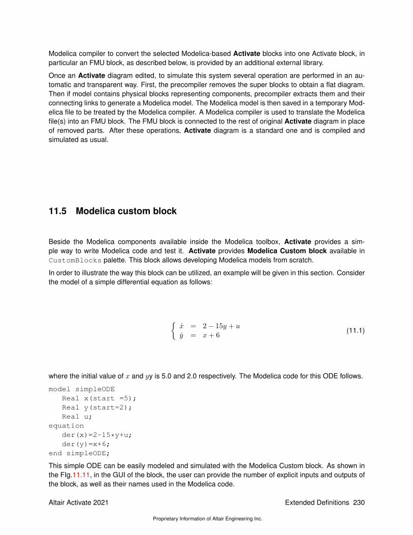
Modelica compiler to convert the selected Modelica-based Activate blocks into one Activate block, inparticular an FMU block, as described below, is provided by an additional external library.
Once an Activate diagram edited, to simulate this system several operation are performed in an au-tomatic and transparent way. First, the precompiler removes the super blocks to obtain a flat diagram.Then if model contains physical blocks representing components, precompiler extracts them and theirconnecting links to generate a Modelica model. The Modelica model is then saved in a temporary Mod-elica file to be treated by the Modelica compiler. A Modelica compiler is used to translate the Modelicafile(s) into an FMU block. The FMU block is connected to the rest of original Activate diagram in placeof removed parts. After these operations, Activate diagram is a standard one and is compiled andsimulated as usual.
11.5 Modelica custom block
Beside the Modelica components available inside the Modelica toolbox, Activate provides a sim-ple way to write Modelica code and test it. Activate provides Modelica Custom block available inCustomBlocks palette. This block allows developing Modelica models from scratch.
In order to illustrate the way this block can be utilized, an example will be given in this section. Considerthe model of a simple differential equation as follows:
x = 2− 15y + uy = x+ 6
(11.1)
where the initial value of x and yy is 5.0 and 2.0 respectively. The Modelica code for this ODE follows.
model simpleODEReal x(start =5);Real y(start=2);Real u;
equationder(x)=2-15*y+u;der(y)=x+6;
end simpleODE;
This simple ODE can be easily modeled and simulated with the Modelica Custom block. As shown inthe FIg.11.11, in the GUI of the block, the user can provide the number of explicit inputs and outputs ofthe block, as well as their names used in the Modelica code.
Altair Activate 2021
Proprietary Information of Altair Engineering Inc.
Extended Definitions 230

Figure 11.11: the GUI of the Modelica custom block for simulating 11.1.
Then in the Simfunction tab of the GUI, the function name and the Modelica code can be given, asshown in Fig.11.12 and Fig.11.13 .
Figure 11.12: the simFunction tab of the GUI of the Modelica custom block for simulating 11.1.
Figure 11.13: The Modelica code for simulating 11.1.
After building the model, as shown in Fig.11.14, it can be simulated. The simulation result is given inFig.11.15.
231 Extended Definitions
Proprietary Information of Altair Engineering Inc.
Altair Activate 2021

Figure 11.14: Complete model for simulation of 11.1.
Figure 11.15: Simulation result for model 11.14.
Note that the input and output ports of this block is explicit and they can be connected to any otherstandard Activate block. In this example, the input u is just a constant block.
Altair Activate 2021
Proprietary Information of Altair Engineering Inc.
Extended Definitions 232

Bibliography
[1] P.Frintzson, Object oriented Modeling and simulation with modelica, Wiley Interscience, 2004.
[2] A. C. Hindmarsh, "LSODE and LSODI, Two New Initial Value Ordinary Differential EquationSolvers", ACM-Signum Newsletter, Vol. 15, 1980, pp. 10–11.
[3] S.E. Mattsson, H. Elmqvist, M. Otter, and H. Olsson, "Initialization of Hybrid Differential-AlgebraicEquations in Modelica 2.0", 2nd Inter. Modelica Conference 2002, Dynasim AB, Sweden and DLROberpfaffenhofen, Germany, 2002, pp. 9–15.
[4] L. R. Petzold, "Automatic selection of methods for solving stiff and nonstiff systems of ordinarydifferential equations", SIAM J. Sci. Stat. Comput., No. 4, 1983.
[5] L. R. Petzold. "A Description of DASSL: A Differential/Algebraic System Solver", In Proceedings ofthe 10th IMACS World Congress, Montreal, 1982, pp. 8-13.
[6] P. N. Brown, A. C. Hindmarsh, and L. R. Petzold, "Consistent Initial Condition Calculation forDifferential-Algebraic Systems", SIAM J. SCI. COMP., NO. 19, 1998.
[7] MASOUD NAJAFI, AZZEDINE AZIL, RAMINE NIKOUKHAH, "EXTENDING SCICOS FROM SYSTEM TO
COMPONENT LEVEL SIMULATION", ESMC2004 INTERNATIONAL CONFERENCE, PARIS, FRANCE,OCTOBER 2004.
[8] MASOUD NAJAFI, SEBASTIEN FURIC, RAMINE NIKOUKHAH, "SCICOS: A GENERAL PURPOSE MOD-ELING AND SIMULATION ENVIRONMENT", MODELICA CONFERENCE 2005, MARCH 7-8, 2005.
[9] MASOUD NAJAFI, RAMINE NIKOUKHAH, SERGE STEER, SEBASTIEN FURIC, "NEW FEATURES AND
NEW CHALLENGES IN MODELING AND SIMULATION IN SCICOS", PROCEEDINGS OF THE 2005 IEEECONFERENCE ON CONTROL APPLICATIONS TORONTO, CANADA, AUGUST 28-31, 2005.
233 Extended Definitions
Proprietary Information of Altair Engineering Inc.
Altair Activate 2021

Altair Activate 2021
Proprietary Information of Altair Engineering Inc.
Extended Definitions 234

Chapter 12
FMI (Functional Mock-up Interface)
12.1 Introduction
Automotive OEMs, who may have several hundreds of suppliers, have difficulties when they need tointegrate many sub-systems from those suppliers.
Since they are specialized sub-systems, such as hydraulics, mechanical, electrical, ... the suppliersuse different modeling and simulation programs for developing their sub-systems or components. Inorder to make sure that all of these subsystems work actually all together, the OEM should simulatethem all together and in combination. For that, the system integrator should be able to work with allprograms and also programs should be able to work with others. This is not of course only a problemin automotive industry but it is prominent in this industry.
A solution would be to share the source code of models and compile them in the host simulator, butvery often these models have proprietary rights and can only be delivered in binary form or as libraries,which means they need special tools.
Co-simulation between simulators is a popular solution to make simulators work together in parallel.This solution works into some extent. In order to implement a co-simulation interface between simula-tors, a specialized interface should be developed. That means an interface per every two simulators.There are many tools and it is usually very hard to replace one by another or do all simulations in asingle tool. There are some programs specialized in Co-Simulation that can interface several simulationtools with several versions, but it is not practically easy to interface all simulation tools.
Developing export and import facilities to exchange models between tools seems also to be a goodsolution, but that needs developing special export and import between tools. Also imported models donot usually work as well as in the original simulator due to difference in the simulator characteristics andlack of a standard format. There are several well-known interface formats, such as Modelica language,s-function from MathWorks, user routines in ADAMS, etc. But most of them are proprietary andcannot be used as standard for communicating between tools.
Even though Modelica is a tool independent language, it cannot be used as a standardized interface formodel exchange because it needs a compiler to convert the language into the executable code.
In 2008, a large number of software and automotive companies as well as several European researchcenters worked in a cooperation project named MODELISAR to create the FMI1 (Functional Mock-up
1More information, Detailed interface specification and images used here can be found at www.fmi-standard.org.
235 Extended Definitions
Proprietary Information of Altair Engineering Inc.
Altair Activate 2021

Interface) standard. The development of the FMI specifications was initiated and coordinated by theDaimler AG company. The FMI standard defines a general interface to other simulators. A component(model) which implements this interface is called FMU (Functional Mock-up Unit). The goal of FMI isthat the calling of an FMU in a simulation environment becomes standardized and remains reasonablysimple. The FMI functions can be imported and called by any external simulation environment such asActivate. The host environment can create one or more instances of the FMU and simulate them. Thisis very similar to the way a model composed of several blocks can be created and simulated in Activate.An FMU may either need a simulation environment to import it and perform numerical integration (FMIfor Model Exchange) or have its own solvers/simulator (FMI for Co-Simulation).
In 2010 the first version of FMI-1.0 for Model Exchange and for Co-Simulation was released[1, 2].
In 2014, FMI-2.0 standard including both Model Exchange and Co-Simulation, was released[3]. FMI-2.0 fixed few issues in FMI-1.0 and is not backward compatible with FMI-1.0. In this document weconcentrate on the FMI-2.0 version. Currently, the development of FMI is conducted by the ModelicaAssociation.
12.1.1 FMI interface types
FMI standard which was introduced to cope with tool interface problems, provides two major solutionsfor interfacing tools:
1. Interface as Model Exchange (in this document often abbreviated as ME): FMI standardizesthe model export as binary or as source code. In this interface type the model can be a systemof algebraic-differential equations (at most index-1 DAE) with discrete equations. With this ap-proach a large range of transient dynamical systems can actually be modeled. In this approach,the numerical solver which is external to the model should be compatible with the model. Thisinterface type will be discussed more in section 12.3.
Figure 12.1: FMI for Model exchange
2. Interface as Co-Simulation (in this document often abbreviated as CS): FMI standardizes theco-simulation between simulation tools. In this interface type, the FMU can contain the model, thenumerical solver, and the simulator. It is also possible that FMU only provide the link between twotools without containing the solver or simulator. In this approach, the tool that imports the FMU,provides the input to the FMU and receives the output of the FMU. This approach is more generaland any kind of simulator and any format such as physical models, 1D-3D and 0D for Controlscan be interfaced. This interface type will be discussed more in section 12.4.
12.1.2 Advantages of using FMI in industry
FMI is a free and open standard published under a BSD license and currently supported by mostimportant actors in the simulation software domain. Up to now more than 70 tools support this standard
Altair Activate 2021
Proprietary Information of Altair Engineering Inc.
Extended Definitions 236
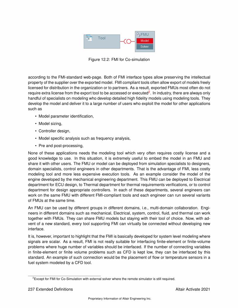
Figure 12.2: FMI for Co-simulation
according to the FMI-standard web-page. Both of FMI interface types allow preserving the intellectualproperty of the supplier over the exported model. FMI compliant tools often allow export of models freelylicensed for distribution in the organization or to partners. As a result, exported FMUs most often do notrequire extra license from the export tool to be accessed or executed2. In industry, there are always onlyhandful of specialists on modeling who develop detailed high fidelity models using modeling tools. Theydevelop the model and deliver it to a large number of users who exploit the model for other applicationssuch as
• Model parameter identification,
• Model sizing,
• Controller design,
• Model specific analysis such as frequency analysis,
• Pre and post-processing,
None of these applications needs the modeling tool which very often requires costly license and agood knowledge to use. In this situation, it is extremely useful to embed the model in an FMU andshare it with other users. The FMU or model can be deployed from simulation specialists to designers,domain specialists, control engineers in other departments. That is the advantage of FMI, less costlymodeling tool and more less expensive execution tools. As an example consider the model of theengine developed by the mechanical engineering department. This FMU can be deployed to Electricaldepartment for ECU design, to Thermal department for thermal requirements verifications, or to controldepartment for design appropriate controllers. In each of these departments, several engineers canwork on the same FMU with different FMI-compliant tools and each engineer can run several variantsof FMUs at the same time.
An FMU can be used by different groups in different domains, i.e., multi-domain collaboration. Engi-neers in different domains such as mechanical, Electrical, system, control, fluid, and thermal can worktogether with FMUs. They can share FMU models but staying with their tool of choice. Now, with ad-vent of a new standard, every tool supporting FMI can virtually be connected without developing newinterface.
It is, however, important to highlight that the FMI is basically developed for system level modeling wheresignals are scalar. As a result, FMI is not really suitable for interfacing finite-element or finite-volumeproblems where huge number of variables should be interfaced. If the number of connecting variablesin finite-element or finite volume problems such as CFD is kept low, they can be interfaced by thisstandard. An example of such connection would be the placement of flow or temperature sensors in afuel system modeled by a CFD tool.
2Except for FMI for Co-Simulation with external solver where the remote simulator is still required.
237 Extended Definitions
Proprietary Information of Altair Engineering Inc.
Altair Activate 2021

Figure 12.3: Using FMUs to share models
12.2 Internal structure of an FMU
An FMU implementing the FMI interface is a model distributed in one zip-file containing several fileswith a structure similar to the diagram shown in Fig.12.4:
Figure 12.4: Internal structure of an FMU.
An FMU is composed of several files that will be discussed as follows:
• An XML file (modelDescription.xml): This XML file contains information on the model and thedefinition of all variables of the FMU in a standardized way. XML file indicates the FMI version,whether the FMU is for Model Exchange and/or for co-simulation, and the features of FMI stan-dard supported by the FMU. The XML file also lists the exposed model variables including inputs,outputs, states, state derivatives, and model parameters. Model parameters can be changed atthe beginning of the simulation of even during the simulation for tunable parameters. An impor-tant information included in the XML is the model structural information, i.e., the variables who areoutput, derivatives, or unknowns at initial time. The dependency of output, derivative and initialunknowns on other variables are also provided. This information is crucial for detecting algebraicloops and correctly handle them in a model aggregated by several FMUs. The XML can alsocontain vendor information. It is important to indicate that information stored in the XML is notneeded for execution of the model. That allows having an executable code with a minimum over-head. Below is an example of an FMI model description issued from Modelica. For more detailson the XML file, interested readers are referred to the section FMI description Schema in
Altair Activate 2021
Proprietary Information of Altair Engineering Inc.
Extended Definitions 238
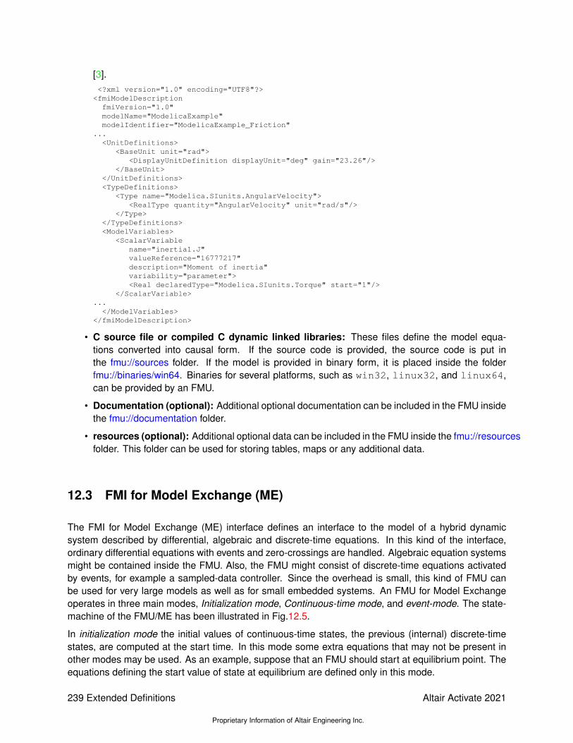
[3].<?xml version="1.0" encoding="UTF8"?><fmiModelDescription
fmiVersion="1.0"modelName="ModelicaExample"modelIdentifier="ModelicaExample_Friction"
...<UnitDefinitions>
<BaseUnit unit="rad"><DisplayUnitDefinition displayUnit="deg" gain="23.26"/>
</BaseUnit></UnitDefinitions><TypeDefinitions>
<Type name="Modelica.SIunits.AngularVelocity"><RealType quantity="AngularVelocity" unit="rad/s"/>
</Type></TypeDefinitions><ModelVariables>
<ScalarVariablename="inertia1.J"valueReference="16777217"description="Moment of inertia"variability="parameter"><Real declaredType="Modelica.SIunits.Torque" start="1"/>
</ScalarVariable>...
</ModelVariables></fmiModelDescription>
• C source file or compiled C dynamic linked libraries: These files define the model equa-tions converted into causal form. If the source code is provided, the source code is put inthe fmu://sources folder. If the model is provided in binary form, it is placed inside the folderfmu://binaries/win64. Binaries for several platforms, such as win32, linux32, and linux64,can be provided by an FMU.
• Documentation (optional): Additional optional documentation can be included in the FMU insidethe fmu://documentation folder.
• resources (optional): Additional optional data can be included in the FMU inside the fmu://resourcesfolder. This folder can be used for storing tables, maps or any additional data.
12.3 FMI for Model Exchange (ME)
The FMI for Model Exchange (ME) interface defines an interface to the model of a hybrid dynamicsystem described by differential, algebraic and discrete-time equations. In this kind of the interface,ordinary differential equations with events and zero-crossings are handled. Algebraic equation systemsmight be contained inside the FMU. Also, the FMU might consist of discrete-time equations activatedby events, for example a sampled-data controller. Since the overhead is small, this kind of FMU canbe used for very large models as well as for small embedded systems. An FMU for Model Exchangeoperates in three main modes, Initialization mode, Continuous-time mode, and event-mode. The state-machine of the FMU/ME has been illustrated in Fig.12.5.
In initialization mode the initial values of continuous-time states, the previous (internal) discrete-timestates, are computed at the start time. In this mode some extra equations that may not be present inother modes may be used. As an example, suppose that an FMU should start at equilibrium point. Theequations defining the start value of state at equilibrium are defined only in this mode.
239 Extended Definitions
Proprietary Information of Altair Engineering Inc.
Altair Activate 2021

Figure 12.5: State Machine for FMI-2.0-Model Exchange.
The continuous-time mode is used to compute the values of all continuous-time variables betweenevents by numerically solving ordinary differential and algebraic equations. All discrete-time variablesare fixed during this phase and the corresponding discrete-time equations are not evaluated.
The Event Mode is used to compute new values for all continuous-time variables, as well as for alldiscrete-time variables that are activated at the current event instant, given the values of the variablesfrom the previous instant. This is performed by solving algebraic equations consisting of all continuous-time and all active discrete-time equations.
The operating mode jumps from continuous-time into event-mode, if an event happens. There are fourevent kinds in FMI:
• State-event (zero-crossing event): Event which is triggered at the time instant where the eventindicator function changes from z > 0 to z ≤ 0, or vice versa. Discontinuities in a model areusually defined as zero-crossing functions (event-indicators).
• Time events: Event that is triggered at a predefined time instant. Since the time instant is knownin advance, the integrator can select its step size so that the event instant is directly reached.Therefore, this event can be handled efficiently.
• Step-event: Event that might occur when the simulator finishes a completed integrator step. Thisevent is not usually defined by the FMU. The simulator may use it, for example, to dynamicallyswitch between different states, or storing data into a file.
• External event: This kind of event is triggered by the environment. This event type is triggeredif at the current time instant, at least one discrete-time input changes its value, a continuous-timeinput has a discontinuous change, or a tunable parameter changes its value.
Upon happening any of these events, the continuous-time integration is stopped and the FMU goes into
Altair Activate 2021
Proprietary Information of Altair Engineering Inc.
Extended Definitions 240

the event-mode.
12.4 FMI for Co-Simulation (CS)
Modeling complex heterogeneous systems in engineering usually leads to hybrid systems of differentialand algebraic system of equations with discrete-time equations. Such complex multi-disciplinary sys-tems cannot often be modeled and simulated in one simulation tool alone. Sub-system models are oftenavailable only for a specific simulation tool. For example special tools for CFD (Computational Fluid Dy-namics) models or integrated circuit systems. In many situations, the sub-systems shall be simulatedwith the simulator which suits best for the specific domain. Thus for the simulation of multi-disciplinarymodels it is often reasonable or even necessary to couple different simulation tools with each otheror with real world system components. Co-simulation is a general approach for the joint simulation ofmodels developed with different tools where each tool treats one part of a modular coupled problem.The data exchange (input and output variables, status information) between sub-systems is restrictedto discrete communication points. In the time between two communication points, the sub-systems aresolved independently from each other by their individual solver.
Main-secondary is a common method in Co-simulation. In a main-secondary approach, the secondarysolvers simulate sub-models whereas the main (solver) is responsible for both coordinating the over-all simulation as well as transferring data. In the main-secondary approach, instead of coupling thesimulation tools directly, it is assumed that all communication (input/output data exchange) is handledvia a main. Main algorithms control the data exchange between sub-systems and the synchronizationof all secondary simulation solvers. Besides distribution of communication data, the main checks theconnection graph, chooses a suitable simulation algorithm and controls the simulation according to thatalgorithm.
The secondary solvers are simulation tools, which are prepared to simulate their subtask. They areable to communicate data, execute control commands and return status information.
FMI for Co-Simulation unifies the main-secondary interface and supports from simple co-simulation al-gorithms to more sophisticated ones. FMI provides a small set of C-functions to implement the interface.It is important to note that the main algorithm itself is not part of the standard FMI for CoSimulation.The main is free to choose the appropriate co-simulation algorithm.
Figure 12.6: Co-simulation with generated code on a single computer.
FMI for Co-Simulation supports two possible ways to provide sub-systems for co-simulation: sub-systems (models) packaged along with their respective solver, which can be simulated as stand-alonecomponents, see Fig.12.6, or a wrapper FMU which calls its respective simulation tool to simulate thesub-system (model), which is installed externally to the FMU, see Fig.12.7. The FMI import in Acti-vate supports both implementations of FMI for Cosimulation. In FMI export in Activate, the solver isembedded in the FMU and no Activate installation is required to run the FMU in other environments.
241 Extended Definitions
Proprietary Information of Altair Engineering Inc.
Altair Activate 2021
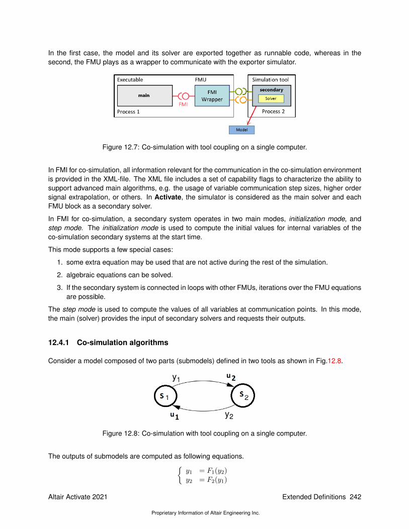
In the first case, the model and its solver are exported together as runnable code, whereas in thesecond, the FMU plays as a wrapper to communicate with the exporter simulator.
Figure 12.7: Co-simulation with tool coupling on a single computer.
In FMI for co-simulation, all information relevant for the communication in the co-simulation environmentis provided in the XML-file. The XML file includes a set of capability flags to characterize the ability tosupport advanced main algorithms, e.g. the usage of variable communication step sizes, higher ordersignal extrapolation, or others. In Activate, the simulator is considered as the main solver and eachFMU block as a secondary solver.
In FMI for co-simulation, a secondary system operates in two main modes, initialization mode, andstep mode. The initialization mode is used to compute the initial values for internal variables of theco-simulation secondary systems at the start time.
This mode supports a few special cases:
1. some extra equation may be used that are not active during the rest of the simulation.
2. algebraic equations can be solved.
3. If the secondary system is connected in loops with other FMUs, iterations over the FMU equationsare possible.
The step mode is used to compute the values of all variables at communication points. In this mode,the main (solver) provides the input of secondary solvers and requests their outputs.
12.4.1 Co-simulation algorithms
Consider a model composed of two parts (submodels) defined in two tools as shown in Fig.12.8.
Figure 12.8: Co-simulation with tool coupling on a single computer.
The outputs of submodels are computed as following equations.y1 = F1(y2)y2 = F2(y1)
Altair Activate 2021
Proprietary Information of Altair Engineering Inc.
Extended Definitions 242

In order to co-simulate this system, this equation should be solved at each communication instant.Fi functions are usually complex, non-linear, and time-dependent relationships, as a result, iterativemethods are the only choice for solving such equations. Three common methods used for solvingthem are Gauss-Seidel and Gauss-Jacobi and Newton methods. The Gauss-Seidel iteration method isrepresented as follows.
yi+11 = F1(y
i2)
yi+12 = F2(y
i+11 )
i = 0, 1, 2, ...
The Gauss-Jacobi iteration method is defined as
yi+11 = F1(y
i2)
yi+12 = F2(y
i1)
i = 0, 1, 2, ...
These iterative methods are simple fixed-point methods and their convergence(at most linear) dependson Fi functions. If the Fixed Point converges very slowly or diverges the Newton-type methods canbe used. These methods are, however, more complicated, because in each step the Jacobian mustbe computed which results in higher number of simulator calls. The method which is used actually inActivate is GS1, i.e., the Gauss-Seidel method with only one iteration. This method has been illustratedin Fig.12.9;
Figure 12.9: Co-simulation method used in Activate.
The simulator of Activate which acts as the main performs the following method for the co-simulationand synchronization between tools, as shown in 12.9.
1. The simulator advances the time from tn to tn+1, and updates the output of all blocks, exceptthose of external tools (secondary). Optionally, the secondary system (FMU) outputs are extrap-olated at a desired order if available from the FMU.
2. External tools are called one by one and asked to advance the their time from tn to tn+1 andtheir output is requested at tn+1. Optionally, the secondary system (FMU) inputs are linearlyinterpolated.
3. The Activate simulator takes a new step from tn+1 to tn+2 using the new output value of sec-ondary systems computed at tn+1.
4. goto 1
243 Extended Definitions
Proprietary Information of Altair Engineering Inc.
Altair Activate 2021

Usually in order to get a correct result, the communication step-size (time instant between two com-munication instants) should not be larger than two times the highest frequency content (one-half thesmallest time constant; Nyquist theorem) of the secondary systems, and in practice should usually besmaller than this. Smaller communication step-size results in better convergence but longer simulationtime. In Activate the user can control the communication step-size, see 12.5.5.
12.4.2 Advanced: FMI import preserving full output/input dependency property
3 A challenge in importing an FMI generated is the treatment of output/input dependencies. In anActivate basic block output/dependencies are expressed as a vector of dependencies specifying theinputs that affect any of the outputs. So the dependency is solely a property of an input port. A basicblock computes all its outputs in the same call, so all its dependent inputs must be up to date whenthe call is made. An FMU, on the other hand, specifies output/input dependencies as matrix specifyingwhich output depends on each input. This input/output dependency matrix may also be different duringthe initialization. It provides routines that allow the computation of output ports separately and takeadvantage of variable caching.
A way to deal with this situation, which was the way Activate imported Modelica parts, is to simply projectthe matrix of dependencies into a vector. This conservative approach properly assigns dependenciesin Activate but "loses" information along the line. This may lead in particular to detection of algebraicloops by the Activate compiler that are not true algebraic loops (artificial algebraic loops). Even thoughthere are ways to break algebraic loops in an Activate model, we decided to detect artificial algebraicloops and treat them properly. A very simple example that illustrates the problem is shown in Figure12.10.
Figure 12.10: A simple model mixing Modelica and Activate blocks
After compiling the Modelica part, a virtual model similar to what is shown in Figure 12.11 is obtained.In the generated FMU, there is a direct dependency between the SignalCurrent input port (in) andthe CurrentSensor output signal (A). The dependency is depicted by a red dashed line if Figure12.11. If the dependency matrix is converted into a vector, output ports A and V depend on input portin. This direct dependency results in an artificial algebraic loop that does not really exist.
In order to solve this problem, the output/input dependency property of the basic blocks can only be setfor ports separately so the imported FMU cannot be represented by a single FMU; but it can be properly
3This section can be skipped without losing the continuity.
Altair Activate 2021
Proprietary Information of Altair Engineering Inc.
Extended Definitions 244

Figure 12.11: The model in Figure12.10, after converting the Modelica part into an FMU block.
represented as a network of basic blocks. The topology of this network depends on the number of inputsand outputs of the FMU and the FMUs output/input dependency matrix. A programmable super blockis thus used for importing the FMU. The block main parameter is the FMU filename. By reading andparsing the XML inside the FMU, the block generates a network of basic blocks, as shown in Figure12.12, during the model compilation stage. The network contains a central basic block, always present,and other blocks associated with each output port. Figure 12.12 illustrates the resulting network for animported FMU with two inputs and four output ports.
Figure 12.12: Automatically generated network of basic blocks from FMU import for an FMU with oneinput and four output ports.
In resulting network of basic blocks, each output unit keeps the direct-feedthrough property of thecorresponding FMU output port. The central unit on the other hand does not have the direct feed-through. In order to communicate within this network, the central block outputs the internal structurewhich contains the FMU context and shares it with other blocks of the network. Note that this processis completely transparent for the user, who never sees the network in Figure 12.12. Hence generatinga programmable network of blocks instead of single block for FMU import, avoids creation of artificialalgebraic loops.
12.5 FMI Import in Activate
Activate can simulate FMI-1.0 and FMI-2.0 block of both Model-exchange and co-simulation kinds. TheFMU Import block (see Fig.12.13) available in the CoSimulation palette is used to import and simulateFMU blocks. This block automatically detects the FMI version and FMI kind and chooses appropriatemethods to simulate them. By double clicking on the block, a block dialog (GUI) is opened as shown inFig.12.14
This dialog allows for selecting and loading an FMU. Once selected, the user can either fill the FMUinformation fields such as number of input and outputs, or click on the Reload button. The button tem-porarily reads the FMU and fills the information fields of the dialog automatically, as shown in Fig.12.15.
245 Extended Definitions
Proprietary Information of Altair Engineering Inc.
Altair Activate 2021

Figure 12.13: FMU Import block from CoSimulation palette
Figure 12.14: Block Dialog for FMU Import (empty)
In the Parameter field, the FMU variables whose start value can be changed are displayed. The usercan provide new values for these variables. The new values are taken into account before the start ofthe simulation.
There are, however, few features of FMI that are not supported by the FMI Import block in Activate.
• Tunable parameters are not supported.
• The FmuSetState and FmuGetState features of FMU are not fully exploited for repeating the stepsand solving algebraic loops.
12.5.1 Direct dependency vector for inputs (Feedthrough)
An FMU block usually provides the dependency of output variables on its variables including its inputvariables. This information is transformed into feedthrough information of the FMU block in Activate(see 9.1.1). This information is displayed in the FMU GUI, as shown in Fig.12.15.. For each input port,a dependency vector is provided which indicates the output ports that depend on the this input port. Inthis vector zero(0) means no dependency and one(1) means direct dependency of output on input.
12.5.2 Advanced tab
Run as "Model Exchange": In FMI-2.0, the FMU can provide both ME and CS implementationsfor a model. In this case, the user can choose the implementation that should be simulated. The "Runas Model Exchange" check-box, if checked, forces the simulator using the Model Exchange implemen-
Altair Activate 2021
Proprietary Information of Altair Engineering Inc.
Extended Definitions 246

Figure 12.15: Graphical user interface of the block FMU-Import (filled)
tation.
Tolerance controlled: This check-box allows choosing if the FMU should be tolerance-controlledor not. If the checkbox is On, then the FMU model is called with a numerical integration scheme wherethe step size is controlled by using the relative error tolerance for error estimation. In such a case, allnumerical algorithms used inside the model operate with an error estimation of an appropriate smallerrelative tolerance. If the fixed-step solver is used, this checkbox may be Off.
Delete the unpacked FMU before exit: The simulator unzips the FMU in a folder on eachrun and deleted the folder once the simulation finished. This check-box allows keeping the folder afterfinishing the simulation.
Show FMU input event ports: This check-box allows displaying/hiding the input event ports ofthe block. The FMU import block has got two input event ports, one for external events and anotherfor End-event. The external event which can be activated by discrete events of Activate pushes theFMU (of type ME) into the event mode. This is important if, for example, the input of the block isdiscontinuous. The End-event pushes the block into the terminate mode, where the output of the blockremains unchanged until the end of the simulation.
Show FMU output event ports: This check-box allows displaying/hiding the output event portsof the block. The FMU import block has got two output event ports, one for discrete event that happeninside the FMU and another for End-event. The discrete event is triggered for example when a timeevent is programmed inside the FMU block. The output End-event is triggered when the FMU requests
247 Extended Definitions
Proprietary Information of Altair Engineering Inc.
Altair Activate 2021

Figure 12.16: Graphical user interface of the block (Advanced tab)
a termination. This event can be used to terminate the simulation.
FMU resource location: This field is used to provide the location of the resource folder to begiven to the FMU. If this field is left empty, the FMU is the default location which is fmu://resources.
Directory for unpacking the FMU: This field allows unzipping the FMU in a specified folder.If this field is left empty, the FMU is unzipped in the temporary folder of Activate.
Run in safe mode: If enabled, the FMU is loaded inside another process. This protects Activatefrom possible crashes in the FMU. The simulation is slower in this mode. Both FMI-1.0 and FMI-2.0 ofModelExchange and CoSimulation kinds can be simulated in this mode.
12.5.3 Reporting tab
FMU interface logging level: The list-box allows choosing the logging level for the interfaceto the FMU block. For example, if the user chooses the Warning level, all logger messages emittedby FMU with status fmi2Warning, fmi2Error and fmi2Fatal will be stored in the logfile. Possible valuesNothing, Fatal, Error, Warning, Info, Verbose.
Enable FMU logging: This check-box enables or disables the whole logger.
Add Activate messages: If this check-box enabled, the messages emitted by Activate interfaceto the FMU will be added to the logfile. If you need to catch only the messages emitted by the FMU,you may turn this checkbox off.
Altair Activate 2021
Proprietary Information of Altair Engineering Inc.
Extended Definitions 248

Figure 12.17: Graphical user interface of the block (Reporting tab)
FMU logging categories (for FMI-2.0): In FMI 2.0, the FMU is given the possibility to filter logger mes-sages. The user can enter the required log categories. Log categories should be protected by doublequote and separated by comma, for example "fmiCall;events;logger2". Only messages with given cate-gories will be stored in the logfile. If left empty, all messages are stored, regardless of their category.
Logfile name (*.log): The log filename to be created. If this field is left empty, no logfile iscreated. stderr as a filename is supported.
Separator character used in CSV file: The separator character in the output CSV file.
Print Enums and Booleans as integers in CSV file: If this check-box is activated,the Enum values are stored as integer, otherwise their text values are stored.
Store only input/output variables: If this check-box is activated, the CSV or HDF file willstore only input and output variables. This allows reducing the result file volume.
Result storage filename(*.csv/*.mtsf): The full path of the output result file. The outputfile can either an CSV file or an HDF file (with extension *.mtsf)[4].
12.5.4 ModelExchange tab
Solver mesh-points events (step events): If checked, whenever a step event happens,the value of variables at that time instant is stored in the CSV file.
Zero-crossing events (state events): If activated, whenever a state event (zero-crossingevent) happens, the value of variables at that time instant is stored.
249 Extended Definitions
Proprietary Information of Altair Engineering Inc.
Altair Activate 2021

Time events: If activated, whenever a time event happens, the value of variables at that time instantis stored.
Every output update: If activated, whenever the block outputs are updated, the value of vari-ables at that time instant is stored.
Meshpoints points: If activated, the value of variables at that solver mesh-points are stored.
Super dense time instants: If activated, the value of variables at super dense time in discreteevent iterations are stored.
12.5.5 CoSimulation tab
Preferred fixed communication step size: An FMU of kind co-simulation is simulated byits internal solver. The FMU and Activate exchange (update) their respective output and input values atintervals called communication points. The interval between communication points is called communi-cation step-size which may vary during the co-simulation. The communication step size can be set bythe "Preferred fixed communication stepsize" parameter in the FMU block under the Co-Simulation tabas shown in Fig.12.18.
Figure 12.18: Setting co-simulation parameters in the FMI import block
The default value is set to zero (0), which means that the communication instants are governed bythe time-step of the Activate solver. Therefore, in order to control the communication interval you canadjust the "maximum step size" parameter for the Activate solver. Note that, if the Activate solver isa fixed-step size solver, the "maximum step size" parameter will be the co-simulation communicationstep size. In Activate, "maximum step size" parameter is found under the Solvers tab of the SimulationParameters dialog.
Alternatively, you can change the "Preferred fixed communication step size" to a non-zero value and thiswill set the rate of communication between the FMU and Activate, regardless of the step-size chosenby the Activate solver. Note that, in this case the communication step size is fixed. If two sub-systems(FMU and Activate part) tightly interact, fixed communication points methods does not work and theco-simulation may diverge. In this case, Newton methods should be employed, although this is not yetsupported in Activate.
FMU Input interpolation: In order to enable the secondary system to interpolate the continu-ous real inputs between communication steps, Activate can provide the first derivatives of the inputswith respect to time using the numerical differentiation method. If this checkbox is activated, the firstderivative of inputs is computed and is given to the FMU. This may be useful if the FMU can exploit thederivative of its input. Note that since the derivative is computed numerically, if the signal is not smoothenough, the computed derivative is poor. In this case the checkbox is better to be off.
FMU Output interpolation: FMU can provide higher order derivatives of their real outputs to
Altair Activate 2021
Proprietary Information of Altair Engineering Inc.
Extended Definitions 250

allow extrapolation of the output variables between communication steps. In order to exploit the deriva-tive and read smoother signal from the FMU, the user can choose the extrapolation order to be used.Based on the chosen extrapolation order, the derivative of outputs of FMU/CS block is used for ex-trapolation of outputs. Note that no extrapolation order bigger what is provided by FMU can be used,otherwise a warning message will be raised. The FMU provides the highest order available and youcan set the extrapolation to this order or any lower order.
Secondary simulator should be visible: If activated, the FMU/CS is co-simulated in in-teractive manner.
12.5.6 Example
In order to demonstrate the way an FMU can be imported, export a model as FMU with another simu-lator, e.g., MapleSim form MapleSoft. You can also choose an FMU from the FMI public SVN server4.Make sure that the FMU you choose is compatible with the Activate binaries. For example if the Acti-vate is compiled for a win64 machine, your FMU should contain win64 DLLs.
Consider for example the bridge rectifier modeled in MapleSim as shown in 12.19. With input signalu = 10 sin(20πt), the simulation result is given in Fig.12.20.
Figure 12.19: A bridge rectifier modeled in MapleSim.
In MapleSim, export this model as FMI-2.0 for ModelExchange or Co-Simulation and load it in Activateas shown in Fig.12.21 and Fig.12.22.
Choose appropriate simulation parameters in Activate, i.e., Final time=1.0, Maximum stepsize=0.0001.and run the model. You should get the same result as in MapleSim, as shown in Fig.12.23.
12.6 FMI export in Activate
Activate can export super blocks as FMI-2.0. The FMU exported in Activate is standalone, i.e., in the4https://svn.fmi-standard.org/fmi/branches/public
251 Extended Definitions
Proprietary Information of Altair Engineering Inc.
Altair Activate 2021

Figure 12.20: Simulation result of model in Fig.12.19 in MapleSim.
form depicted in Fig.12.6. In the FMU, the numerical solver used in the model setting is embedded inthe FMU. So no Activate installation is required to run the FMU in other environments.
In order to export a model or a part of a model, the interested region should first be placed into a superblock. Once converted into a super block, in the Tools/FMU 2.0 drop down menu, select the exportmethod: either Model Exchange, Co-Simulation, or both can be selected as an option to export an FMU.The name and identifier of the exported FMU will be the name of the super block. Hence, if the name ofthe super block contains unsupported characters, they are converted to "_". For example if the nameof the super blocks is "SuperB !%lock", "sb_SuperB___lock" will be used instead. After theFMU generation, the user is asked to select a folder to save the generated FMU. The default locationis next to the model. If the super block is exported as FMI for co-simulation, the Activate simulator aswell as the simulation parameter values in the "setup" menu will be used in the exported model. If amodel is implicit, i.e., contains implicit blocks, such as ImplicitDerivative, Constarint, or Automaton, itcan only be exported as FMU for CoSimulation. In this case, an implicit solver such as, Ida, Daskr, orRadau(DAE) is used inside the FMU.
12.6.1 Nested FMU
A superblock containing other FMUs (FMI-1.0 or FMI-2.0 of kind ModelExchnage or cosimulation) canbe exported as a new FMU.
12.6.2 Exporting Modelica
A superblock containing Modelica components can be exported as FMU. Note that the superblockcannot have Modelica ports (implicit Activate ports). All input and output ports should be of explicitsignal type to be exported as FMU.
Altair Activate 2021
Proprietary Information of Altair Engineering Inc.
Extended Definitions 252

Figure 12.21: FMI Block dialog in Activate
Figure 12.22: Bridge model (bridge.scm)
12.6.3 Shortcomings
Current version of the FMI export of Activate does not support following features:
• Signal import blocks FromBase and SignalIn are not supported.
• Signal export blocks ToBase and SignalOut are not supported.
• Signal Viewer blocks such as Scope, Display, etc. are ignored.
• Co-simulation blocks such as MotionSolve or Flux blocks are not supported.
• Memory block is not supported.
12.6.4 Requirements
The FMI export facility needs a MicroSoft Visual Studio C++ compiler installed on the system. Otherwisethe generated C code cannot be compiled and no binary will be available for the FMU and FMI export
253 Extended Definitions
Proprietary Information of Altair Engineering Inc.
Altair Activate 2021

Figure 12.23: Result in Activate.
fails. Note that Activate automatically detects the C compiler on the system. In order to detect the Ccompiler, you may use the command: vssGetCompilerName()
Note that the tcc compiler cannot be used in FMI export.
12.6.5 Example
In order to demonstrate the way a model in Activate can be exported, here is an example. Open themodel Controller_Me_CS.scm available in the product installation directory, under tutorial_models/Extended_Book_Models/Chapter_11_FMIfolder. Suppose that we want to export the indicated region in the model, as shown in Fig.12.24.
Figure 12.24: Controller model (AFM_controller.scm)
• Select the region and convert it into a super block as shown in Fig.12.25. Rename the superblock as needed to the name of the FMU to be generated.
Altair Activate 2021
Proprietary Information of Altair Engineering Inc.
Extended Definitions 254

Figure 12.25: Controller model after superblock creation (SFM_controller.scm)
• If the superblock contains Input ports, inside the super block, click on the Input blocks and activatethe "Time-Dependency" checkbox and fill the input dimensions with correct values (as shown inFig.12.26). Otherwise an FMU with only discrete-time variables will be generated and the size ofinput ports will be one.
• Get outside of the super block and after selecting the super block, select the menu Tools/FMU2.0 and choose the export type: Model Export, Co-Simulation, or both.
• The C code and the binaries are generated in the Activate model temporary folder.
• Once the FMU is generated, a dialog window opens and asks the user to choose a folder to copythe FMU into.
• The generated FMU can be imported as an FMU with the "FMI import" block and be tested toverify if it gives the same result.
Figure 12.26: Input-port block dialog.
12.7 Advanced user topics:
The co-simulationalgorithm is not a part of the FMI standard and tools are free to choose the bestmethod to perform the co-simulation with an FMU. The FMI import block is basically an Activate blockthat interfaces an FMU (ModelExchange or CoSimulation) with Activate. Similar to any other Activateblock, the FMI import block is called with several flags during the simulation. The model is updatedthrough the propagation of block outputs throughout the whole model. In the output propagation, theinput/output dependency of the blocks plays an important role. For example, if at least one output ofa block depends directly on the ith input of the block, the block is not called (i.e., its outputs are notupdated) unless ith input is updated. This is guaranteed by the Activate compiler to ensure that at
255 Extended Definitions
Proprietary Information of Altair Engineering Inc.
Altair Activate 2021

any time instant and for a given continuous-time state, the outputs are correctly evaluated. Once allinput and outputs are evaluated, other jobs, like reading derivative of continuous-time states, evaluatingthe zero-crossing surfaces, programming a discrete event, or in the case of co-simulationwith an FMUcalling fmixDoStep can be done. For more details about the simulation flags and calling blocks thereader is referred to the chapter 9.
For the sake of simplicity, consider an Activate model containing only one FMU, as shown in Fig-ure12.27. The FMU has only one input and one output port. The whole Activate part is abstractedinto a single block. In co-simulation, the standard part of the Activate model and the FMU exchange
Figure 12.27: Simple co-simulationmodel
their input and output signals at some time instants called communication points (CP). Between twosubsequent CPs Activate simulator engine and FMU simulate separately with their respective solver.At the communication step ti, the Activate simulator engine takes the lead and performs the simulationuntil the next communication step, i.e., simulate the interval [ti, ti+1]. During the integration between tiand ti+1, the outputs of the FMU can be extrapolated. Mathematically speaking, the Activate simulatorengine performs the simulation of this model for the interval ti ≤ t ≤ ti+1,
xA = f(xA, uA(t))
uA(t) = yF (ti) + (t− ti)y′F (ti) + (t−ti)22 y′′F (ti) + ...
(12.1)
where xA is Activate continuous-time states and uA is the input of the Activate part. yF , y′F and y′′Fare output of the FMU block, and their first and second time derivatives, respectively. If extrapolation isdisabled (i.e., zero order extrapolation method is selected) then uA(t) = yF (ti).
During the integration of the Activate part, the FMU may be invoked several times to retrieve yF (ti),y′F (ti),y′′F (ti) , etc.
Once Activate engine simulated the interval [ti, ti+1], and yA(ti+1) is evaluated, it is the FMU turn toadvance and simulate the same interval. Right before invoking fmixDoStep, the input values of theFMU at ti (i.e., uF (ti) and possibly its first order derivative ( i.e., der(UF (ti))) are given to FMU (usingfmi2SetXXX and fmi2SetRealInputDerivatives commands). Also, the value of uF (ti+1) is
Altair Activate 2021
Proprietary Information of Altair Engineering Inc.
Extended Definitions 256
read and saved for subsequent fmixDoStep calls.
The derivative of input is computed as follows:
der(UF (ti)) =uF (ti+1)− uF (ti)
ti+1 − ti
Once FMU inputs are set, the FMU is called to perform fmixDoStep(cp=ti, h=ti+1 − ti).
Controlling the co-simulationcommunication step
In the co-simulation with an FMU, the size of communication steps is governed by the numerical solverof Activate (see the model settings panel). If a variable step-solver is chosen, the communication stepwill be variable and with a fixed-step solver, the communication steps will be fixed. In some cases, thisbehavior is not desired. Consider, for example, a complex Activate model where a variable step-solveris needed but calling fmixDoStep in an FMU is costly. In this case, the user has the possibility ofchoosing a fixed-communication step size in the FMU parameter settings (section 12.5.5) .
Unlike the variable communication step size where every Activate numerical solver step is followed by afmixDoStep in the FMU, if a fixed-Communication step is chosen by the user, fmixDoStep is calledperiodically, regardless of Activate Solver steps. Upon dependence of the output of the FMI block onthe rest of the model, Activate solver meshpoint may or may not coincide with the communication pointsof FMI. For example, if the output of the FMI block does not go to any block with continuous-time state,the solver mesh-point and communication points do not coincide.
Calling fmixDoStep
As described in section 12.4.1, Activate and the FMU for co-simulation alternate between calling theirrespective solvers to solve and advance time between communication points and coupling shared data(inputs/outputs) at these communication points. At any particular time (ti), Activate will take a timestep from ti to ti+1 first and then call to the FMU to advance the time with fmixDoStep. Activatecalls fmixDoStep for either the flag VssFlag_OutputUpdate or VssFlag_EventSchedulingdepending on the model and FMU parameter settings.
Blocks in Activate are called in a predefined order with flag VssFlag_OutputUpdate, in order toread the output ports. The simulator propagates the updated output port values all over the model.Once all input and output ports of blocks are updated, the blocks can be called (maybe in an arbitraryorder) to do the update job with flag VssFlag_EventScheduling and VssFlag_StateUpdate(see the section 9.1.1 for more details).
In one case for calling DoStep in FMU for co-simulationblocks, after the input/output update phase atti+1, the input value of the FMU block at ti (and possibly their derivatives) are given to the FMU. ThenfmixDoStep is called in flag VssFlag_EventScheduling to advance the FMU time from ti toti+1
5.
It is important to note that if fmixDoStep is called in flag VssFlag_EventScheduling, the outputof the FMU are not immediately read because this is the purpose of the flag VssFlag_OutputUpdatewhich was called prior to VssFlag_EventScheduling. The outputs of the FMU will be updated inthe next model input/output update with flag VssFlag_OutputUpdate .
5The flags and the job that the block should do in each flag has been explained in chapter 9
257 Extended Definitions
Proprietary Information of Altair Engineering Inc.
Altair Activate 2021

This usually introduces a communication step delay in the output signal versus the input signal. Insome situations, it is possible to perform fmixDoStep during the input/output update phase, i.e.,with flag VssFlag_OutputUpdate . In this case, the newly updated output can be propagatedthrough the model and the delay be avoided. The situations where fmixDoStep will be called in flagVssFlag_OutputUpdate are:
• If the FMU block does not have any input port, no need to wait all input/output update propagationto call fmixDoStep. At the block invocation to retrieve uA(ti+1) (which is equal to yF (ti)),fmixDoStep will be called and immediately yF (ti+1) can be obtained and propagated into themodel. In this way, the delay is avoided.
• If the variability of all inputs is discrete or none of input data-types is Real, uF (t) will be equalto uF (ti) all over the interval [ti, ti+1]). As a result, fmixDoStep will be called at input/outputupdate with flag VssFlag_OutputUpdate .
• If the input interpolation is off or the FMU does not support interpolation, uF (t) will be equalto uF (ti) all over the interval [ti, ti+1]). As a result, fmixDoStep will be called at input/outputupdate with flag VssFlag_OutputUpdate .
• Once all input values of FMU at ti+1 are read during the input/output update phase with flagVssFlag_OutputUpdate. As an example, consider the case where an output of the FMUdepends directly on all input ports of the FMU. Once the value of the output port is requested bythe simulator, it means that all inputs are already updated by the simulator at ti+1. As a result,fmixDoStep can be immediately called and the FMU output yF (ti+1) can be propagated for theFMU outputs whose value are not already propagated.
Input interpolation and output extrapolation in co-simulation
Activate is a hybrid simulation tool which means it can simulate a model with continuous-time anddiscrete-time parts. The discrete-time part is activated by discrete-time events and the continuous-time part of the model is integrated by the numerical solvers of Activate. Discrete-time events causediscontinuities in signals. As a result, signals in a hybrid model may be piece-wise continuous. Sinceseveral discrete-time events may happen at the same time, a signal may have several values at thesame time instants, as shown in Fig.12.28.
Figure 12.28: evaluation of a model at different time instants
The multiple time instants at an event time is also called super dense time instants. During the integra-tion of the continuous-time part, the numerical solver takes steps to advance the time. At the beginningof each step, the time dependent part of the model are evaluated with the flags VssFlag_OutputUpdate,VssFlag_EventScheduling and VssFlag_StateUpdate . The time instant where the modelis evaluated at the beginning of the solver step is also called a solver ’mesh-points’. Discrete-time
Altair Activate 2021
Proprietary Information of Altair Engineering Inc.
Extended Definitions 258

events are classified in two categories, critical and non-critical events. Critical events are discrete-timeevents that may cause discontinuities in the continuous-time part of the model. If a critical event hap-pens, the numerical solver needs to be cold-restarted6. Following one or several critical events, there isalways a solver mesh-point to update the continuous-time parts. In other words, after the evaluation ofa model at critical events, the continuous-time part should be evaluated before starting the integrationof the continuous-time part. Unlike critical events, after a non-critical events, there is not necessarily amesh-point. Non-critical events may happen between two mesh-points.
If the "Preferred fixed communication stepsize" in the co-simulation tab of the FMU block, is left zero,then the Activate solver mesh-points are taken as the co-simulation communication points, i.e., inFig.12.29 ti and ti+1 are Activate mesh-points and also communication points. Since the model mayhave critical events, the model may get evaluated several times at communication instants. Before call-ing fmixDoStep at the mesh-point ti+1, the input of the FMU at the mesh-point (i.e., uF (ti)) is givento the FMU. If the derivative of the input is also provided to the FMU, Activate computes the first orderderivative of the input by using the following equation.
der(uF (ti)) =uF (ti+1)− uF (ti)
ti+1 − ti
Note that in order to compute the derivative of the input, the input value at the mesh-point evaluation,as well as the first super dense time at the next communication points is used, see Fig.12.29.
Figure 12.29: First order interpolation of FMU inputs in presence of events at communication steps.
If the "Preferred fixed communication stepsize" in the co-simulation tab of the FMU block is non-zero,then the communication points are periodic. i.e., in Fig.12.30, ti and ti+1 are communication points.Between communication points, there may be several Activate mesh-points, see Fig.12.30. The FMUis activated by a periodic events where at each event time, fmixDoStep is called. In this case, beforecalling fmixDoStep at the event time of ti+1, the input of the FMU at the previous communicationpoint (i.e., uF (ti)) is given to the FMU.
Figure 12.30: First order interpolation of FMU inputs in presence of events at communication steps(fixed communication step).
6For more details about events, and solver, interested readers are referred to the chapter on solvers.
259 Extended Definitions
Proprietary Information of Altair Engineering Inc.
Altair Activate 2021
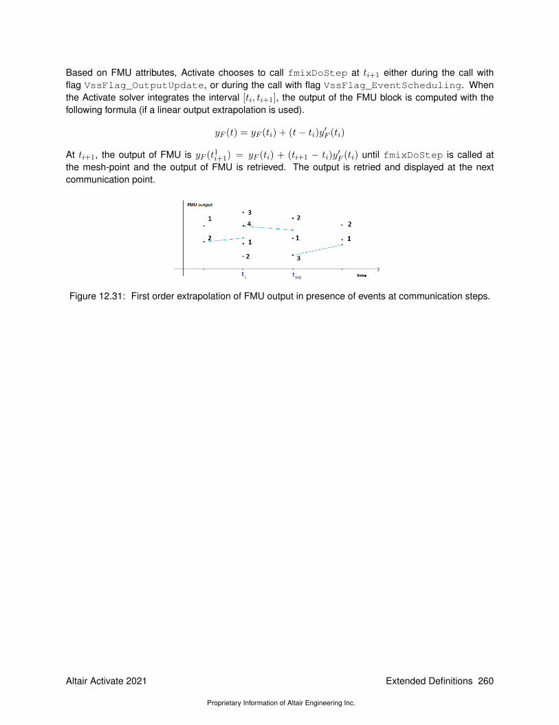
Based on FMU attributes, Activate chooses to call fmixDoStep at ti+1 either during the call withflag VssFlag_OutputUpdate, or during the call with flag VssFlag_EventScheduling. Whenthe Activate solver integrates the interval [ti, ti+1], the output of the FMU block is computed with thefollowing formula (if a linear output extrapolation is used).
yF (t) = yF (ti) + (t− ti)y′F (ti)
At ti+1, the output of FMU is yF (t1i+1) = yF (ti) + (ti+1 − ti)y′F (ti) until fmixDoStep is called at
the mesh-point and the output of FMU is retrieved. The output is retried and displayed at the nextcommunication point.
Figure 12.31: First order extrapolation of FMU output in presence of events at communication steps.
Altair Activate 2021
Proprietary Information of Altair Engineering Inc.
Extended Definitions 260

Bibliography
[1] Functional Mock-up Interface for Model Exchange. Version-1.0, 2010.
[2] Functional Mock-up Interface for Co-Simulation. Version-1.0, October 2010.
[3] Functional Mock-up Interface for ModelExchange and Co-Simulation, Version-2.0, 2014.
[4] Proposal for a Standard Time Series File Format in HDF5, Andreas Pfeiffer,Ingrid Bausch-Gall,Martin Otter, LinkÃuping Electronic Conference Proceedings, 2012.
[5] A Simulation Environment for Efficiently Mixing Signal Blocks and Modelica Components,RamineNikoukhah,Masoud Najafi,Fady Nassif, Modelica Conference, Prague, 2017
261 Extended Definitions
Proprietary Information of Altair Engineering Inc.
Altair Activate 2021

Altair Activate 2021
Proprietary Information of Altair Engineering Inc.
Extended Definitions 262

Chapter 13
Co-Simulation with Multi-body Simulation
13.1 Introduction
Modeling complex heterogeneous systems in engineering usually leads to hybrid systems of differentialand algebraic system of equations with discrete-time equations. Such complex multi-disciplinary sys-tems cannot often be modeled and simulated in one simulation tool alone. Subsystem models are oftenavailable only for a specific simulation tool. For example special tools for CFD (Computational Fluid Dy-namics) models or integrated circuit systems. In many situations, the sub-systems shall be simulatedwith the simulator which suits best for the specific domain. Thus for the simulation of multi-disciplinarymodels it is often reasonable or even necessary to couple different simulation tools with each otheror with real world system components. Co-simulation is a general approach for the joint simulation ofmodels developed with different tools where each tool treats one part of a modular coupled problem.The data exchange (input and output variables, status information) between subsystems is restrictedto communication points. In the time between two communication points, the subsystems are solvedindependently from each other by their individual solvers. If intermediate input or output are needed byone of simulators, it is very often computed through interpolation or extrapolation.
Main-Secondary is a common method in Co-simulation. In a main-secondary approach the secondarysolver simulates the sub-model whereas the main solver is responsible for both coordinating the overallsimulation as well as transferring data. The secondary solvers are the simulation tools, which areprepared to simulate their subtask. The secondary solvers are able to communicate data, executecontrol commands and return status information. Several MSplant blocks representing different AltairMotionSolve models can be instantiated in an Altair Activate model.
13.2 Co-Simulation with MBS
The Co-simulation interface lets the user simulate a complex system that includes one or more multi-body systems (defined by MotionSolve blocks) and several subsystems modeled with Activate blocks.In order to effectively simulate the entire system, the MBS subsystems are simulated with MotionSolvemodels 1 while the control subsystem is simulated with Activate.
1The installation of Altair MotionSolve TM software is required for co-simulation. MotionSolve is a multi-body model-ing, analysis, visualization and optimization solution for performing multi-disciplinary simulations that include kinematics anddynamics, statics and quasi-statics, linear and vibration studies, stress and durability, loads extraction, co-simulation, effort
263 Extended Definitions
Proprietary Information of Altair Engineering Inc.
Altair Activate 2021

In the Activate-MotionSolve interface, Activate is the main solver and MotionSolve (MS) is secondarysolver. The co-simulation interface has been implemented in a block called MS Plant which is availablein the Advanced/CoSimulation palette, as shown in Fig.13.1. MS Signals is a variant of MS Plantblock that displays the name of MS signals at the input/output ports of the blocks.
Figure 13.1: Blocks in Activate to simulate a MotionSolve model.
The block provides a small set of C++ functions to implement the Activate-MotionSolve interface. Thepath of the MotionSolve model is given to MS Plant and MotionSolve solver is called to simulatethe model. In order to perform the simulation, it is necessary to have MotionSolve installed on themachine. This process is shown in fig.13.2.
Figure 13.2: Co-simulation between Activate and MotionSolve.
The co-simulation connection variables to define the inputs/outputs from the MotionSolve model aredefined within the Control_PlantInput and Control_PlantOutput MotionSolve statements, which is a listof runtime (solver) variables for inputs and outputs to the mechanical plant, respectively. These alsohave settings for the hold_order, sampling_period, and offset_time.
In co-simulation, after instantiation and initialization of the MotionSolve solver, inputs to the Motion-Solve model is provided and the output of the MotionSolve block is requested. In order to explain theway a co-simulation is performed, consider a model composed of two simulators as shown in Fig.13.3.
If the output of each model is computed as following equations:yact = Fact(yms)yms = Fms(yact)
in order to co-simulate this system, this equation should be solved at each communication instant.Fi functions are usually complex, non-linear, and time-dependent relationships, as a result, iterativemethods are the only choice for solving such equations. Three common methods used for solvingthem are Gauss-Seidel and Gauss-Jacobi and Newton methods. The Gauss-Seidel iteration method is
estimation and packaging synthesis.
Altair Activate 2021
Proprietary Information of Altair Engineering Inc.
Extended Definitions 264

Figure 13.3: Co-simulation between Activate and MotionSolve
represented as follows.yi+1act = Fact(y
ims)
yi+1ms = Fms(y
i+1act )
i = 0, 1, 2, ...
The Gauss-Jacobi iteration method is defined as
yi+1act = Fact(y
ims)
yi+1ms = Fms(y
iact)
i = 0, 1, 2, ...
These iterative methods are simple fixed-point methods and their convergence(at most linear) dependson Fi functions. If the Fixed Point converges very slowly or diverge the Newton-type methods can beused. These methods are, however, more complicated, because in each step the Jacobian must becomputed which results in higher number of simulator calls. Activate does not support roll back in time,as result, the method which is used actually in Activate is GS1, i.e., the Gauss-Seidel method with onlyone iteration. In this CoSimulation scheme there is no error control.
This method has been illustrated in Fig.13.4;
Figure 13.4: CoSimulation method used in Activate.
The Activate simulator performs the following steps for the co-simulation and synchronization betweensecondary solvers, as shown in 13.4.
1. The Activate simulator advances the time from tn to tn+1, and updates the output of all blocks(except secondary solvers).
265 Extended Definitions
Proprietary Information of Altair Engineering Inc.
Altair Activate 2021

2. Secondary solvers are called one by one and asked to advance their time from tn to tn+1 andtheir output is requested at tn+1.
3. The Activate simulator takes a new step from tn+1 to tn+2 using the new output value of sec-ondary solvers computed at tn+1.
4. Goto 1
Usually in order to get a correct result, the communication step-size (time between two communicationinstants) should not be larger than the smallest time-constant of secondary solvers. Often smallercommunication step-size results in better convergence but longer simulation time.
During the CoSimulation, Activate is the lead solver and takes the lead and advances the time, asshown in 13.4. Once Activate took its step and reached tn+1, then MotionSolve solver which is thelag solver takes its own internal steps to reach at least tn+1.
13.2.1 Under the hood
The CoSimulation method shown in 13.4 is a rough representation of the CoSimulation method betweenActivate and MotionSolve. Actually, on the MotionSolve side there are two buffers for keeping inputand output values exchanged at communication points, tn, tn+1, etc. , as shown in 13.5.
Figure 13.5: Input and output buffers in MotionSolve.
1. Input-buffer: At communication points tn, Activate deposits the inputs to MotionSolve into thisbuffer whenever Activate calls the MotionSolve block. The deposit time instants are completelyindependent of MotionSolve internal steps. MotionSolve solver can query this buffer to get thedata it needs at a specific time. Since the MotionSolve solver is the lag solver, the input bufferwill always interpolate the data deposited by Activate to provide the input to the MotionSolvesolver. The interpolate order is 2.
2. Output-buffer: MotionSolve deposits the outputs from MotionSolve into this buffer at the fre-quency it is supposed to. The deposit time instants are completely independent of Activateinternal steps or communication points. Activate solver can query this buffer to get the data itneeds at a specific time. Since Activate is the lead solver, the output buffer will extrapolate atcommunication points tn < t ≤ tn+1 to provide the output to the Activate solver. The order of
Altair Activate 2021
Proprietary Information of Altair Engineering Inc.
Extended Definitions 266

extrapolation is defined in the MotionSolve xml model, as will be explained as follows.
The writing into and reading from these buffers follows three basic rules in MotionSolve:
1. At each step for any solver, either Activate or MotionSolve, makes an attempt to deposit datainto its corresponding output buffer, i.e., output-buffer for MotionSolve and input-buffer forActivate, and the output buffer immediately returns the control back to the solver. The data isaccepted if the step is a successful step, and rejected if it’s not. Then, the solver will request datafrom its input buffer.
2. When input buffer gets request from a solver, the MotionSolve solver will need to wait if there isnot enough data for interpolation. The Activate solver has to wait if the request time is more thanone step (the Activate solver’s step) larger than the last time the MotionSolve solver made anattempt to deposit or request data to the same buffer.
3. A buffer-in-use lock should be enforced to prevent buffer from being overwritten (by new deposit)while the same buffer is preparing and returning request for another solver.
In general, one should choose Activate solver to be the solver with smaller stepsize and MotionSolveto be the solver with larger stepsize. This is because Activate solver usually gets extrapolated inputsand MotionSolve always gets interpolated inputs, and extrapolating by a large step usually leads toworsen results. Also, the inputs to the Activate solver should be something less prone to noise, like dis-placements. The inputs to the MotionSolve solver, on the other hand, can be less restrictive includingnoisier signals such as forces or torques.
When the Activate solver requests the output-buffer the output at tn, the MotionSolve solver cannotintegrate beyond tn. Actually, whether MotionSolve solver can integrate beyond tn or not is not de-termined by when the Activate solver requests the output-buffer for a data. It is determined by whenthe last time Activate solver deposits a data at the input-buffer. Since, this last time is usually tn, Mo-tionSolve solver cannot integrate beyond this point because the input-buffer will keep the MotionSolvesolver waiting until there is enough data for interpolation (rule #2).
These two buffers are not visible from Activate’s side and filled and queried only by MotionSolve.Activate communicates with MotionSolve only at communication points tn. When outputs of the Mo-tionSolve block are computed at communication points, MotionSolve extrapolates the outputs. Theorder of extrapolation, is defined by the parameter HOLD_ORDER defined in the MotionSolve or Mo-tionView model. This parameter which defines the degree of the polynomial used for extrapolation takesthe following values:
1. HOLD_ORDER = 0 means the last value is returned.
2. HOLD_ORDER = 1 means a straight line is fitted through the last 2 points. The line is extendedto the new time to return the signal value.
3. HOLD_ORDER = 2 means a parabola is fitted through the last 3 points. The parabola is extendedto the new time to return the signal value.
4. HOLD_ORDER > 2 is not supported, because extrapolation is inherently dangerous and higherorder extrapolations can lead to large (and unexpected) values.
The decoupling of the solvers through the buffer mechanism allows each solver to pick its own step. Inother words, Activate and MotionSolve solver settings do not directly affect each other’s time steps.This leads to a faster simulation. The only way the simulators can affect each other’s time step is throughthe model. If the MotionSolve output is smooth enough, that will allow Activate’s numerical solver takelarger step sizes. On the other hand, if in the MotionSolve side, a lower order extrapolation order is
267 Extended Definitions
Proprietary Information of Altair Engineering Inc.
Altair Activate 2021

chosen or the MotionSolve output shows noisy or high frequency behavior, the Activate numericalsolver needs to choose smaller steps to reduce the error. When MotionSolve output is noisy, data gotfrom 2nd order extrapolation at larger time step will be way off. This is the reason that user needs tochoose order 1 or 0. So, in the MotionSolve xml, a lower extrapolation order needs to be chosen whenthe MotionSolve output shows noisy or high frequency behavior, otherwise the Activate numericalsolver needs to choose smaller steps to reduce the error.
Interested users are referred to the MotionSolve Users Guide for more information.
13.3 MSplant block parameters
The MSplant block implements co-simulation interface between Activate and MotionSolve. Simula-tions with this block require that Altair MotionSolve solver is installed. The path to the solver and itslicensing must be set within Activate preferences panel, section Co-Simulation.
Figure 13.6: Graphical user interface of the MSplant block.
• XML or MDL input filename: In this field the name of the MotionSolve model (with extension.xml) or MotionView (with extension .mdl) can be given. The filenames can be either given by anabsolute path, or a relative path. If Activate and MotionSolve models are in the same folder, nopath is required. In the later case the absolute path is obtained from where the Activate modelis located. If a MotionView is given the (.mdl) file is automatically converted into a MotionSolve(.xml) file.
• Launch MotionView: If a MotionView (.mdl) file is provided as the input MotionSolve filename,it is possible to visualize and edit the model in MotionView by clicking on this button. Note: WhenMotionView is open Activate remains inactive.
Altair Activate 2021
Proprietary Information of Altair Engineering Inc.
Extended Definitions 268

• MRF output filename: This field indicates the name of the MotionView result filename. Note thatthe folder where is file should be generated is not write-protected. If the corresponding feature isactive in the MotionSolve (.xml) model, the MotionView result file (.mrf) will be converted into anH3D file (.h3d). The .mrf and .h3d files can be visualized in MotionView.
• DLL User-sub filename (optional): If the MotionSolve model requires extra libraries for execu-tion, the path of these DLLs can be provided in this field. The DLLs provided here will be loadedby MotionSolve at the beginning of the co-simulation and will be released at the end.
• Number of input ports: The number of input ports of the block. This number must correspondto the number of plant inputs in the MotionSolve model. This field is automatically filled if theReload button is pressed.
• Inputs: Each row corresponds to an input port. The label of input as well as the size of the inputshould be provided here. These fields are automatically filled if the Reload button is pressed.
• Number of output ports: The number of output ports of the block. This number must correspondto the number of plant outputs in the MotionSolve model. This field is automatically filled if theReload button is pressed.
• Outputs: Each row corresponds to an output port. The label of output as well as the size ofthe output should be provided here. These fields are automatically filled if the Reload button ispressed.
• Direct feedthrough: The MotionSolve model does not indicate if an input of the MSplantblock directly affects the outputs (feedthrough information). This check box allows setting thefeedthrough value. If this check-box is active, it is ensured that the input of the block is always up-to-date when the output of the block is requested. Otherwise a very short delay may be observedin the output of the block.
• Reload button: The information about the input and output of the MotionSolve model and theirnames and their sizes are all available in the MotionSolve (.xml) file. Instead of filling the abovefields manually, the user can fill them automatically by pressing this button. Filling manually thefields is useful when the xml file is not still available and the user needs to build the Activatemodel.
• MotionSolve server IP address: This field is not currently used.
• MotionSolve server port number: This field is not currently used.
13.4 Example: Pendulum Swing-Up
The inverted pendulum is a popular system for illustrating control and multi-body problems. In [1], acontrol strategy for swinging up a pendulum from downward position to the upright position has beenpresented. This strategy has been explained and implemented in 16.3.1 where the pendulum and thecontroller are implemented in Activate. Here we will explain the way the pendulum is implemented inMotionSolve and the controller in Activate. The resulting models are then co-simulated to bring thependulum in upward position.
The inverted pendulum has been implemented in MotionSolve as shown in Fig.13.7. This model isavailable as a Activate model in the Main_Demos folder. The model has one input signal sa_in[1]of size one and one output vector signal sa_out[3] of size three, as shown inFig.13.8. The force
269 Extended Definitions
Proprietary Information of Altair Engineering Inc.
Altair Activate 2021

Figure 13.7: Model of inverted pendulum on a cart realized in MotionSolve.
applied to the pendulum cart’s translational y-axis the input signal to the MSâAZ model (force.y (u)),as shown in Fig.13.9.
The output signals used which go to Activate are
• angle_ball_globalz(θ),
• omega_ball_globalz(ω),
• cart.y(y)
as shown in Fig.13.10.
The controller is much easier to implement in Activate, because it is a more adapted tool for buildingcomplex controllers. The controller which receives the angle and the angular velocity of the pendulumhas been implemented in Activate, as shown in Fig.13.13. The block parameters of the MSplant blockis shown in Fig.13.12. The co-simulation result is shown in Fig. 13.14. The evolution of pendulum angleand angular velocity (θ and ω) are given in the first and the second subplots, respectively. The thirdsubplot is the cart displacement which is not controlled. The fourth subplot is the input signal to theMSplant block (applied axial force to the pendulum).
Altair Activate 2021
Proprietary Information of Altair Engineering Inc.
Extended Definitions 270

Figure 13.8: Input and output variables of the MotionSolve pendulum model.
Figure 13.9: Input variable of the MotionSolve pendulum model.
Figure 13.10: Output variables of the MotionSolve pendulum model.
271 Extended Definitions
Proprietary Information of Altair Engineering Inc.
Altair Activate 2021
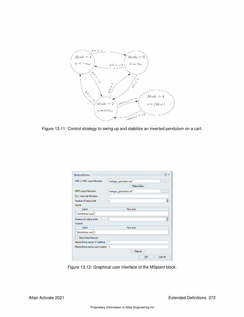
Figure 13.11: Control strategy to swing up and stabilize an inverted pendulum on a cart.
Figure 13.12: Graphical user interface of the MSplant block.
Altair Activate 2021
Proprietary Information of Altair Engineering Inc.
Extended Definitions 272

Figure 13.13: The controller built in Activate.
Figure 13.14: The co-simulation result displayed in Activate.
273 Extended Definitions
Proprietary Information of Altair Engineering Inc.
Altair Activate 2021

Altair Activate 2021
Proprietary Information of Altair Engineering Inc.
Extended Definitions 274

Bibliography
[1] Swinging up a pendulum by energy control, K. J. Astrom and K. Furuta, Automatica, Volume 36, pp278-285, 2000.
275 Extended Definitions
Proprietary Information of Altair Engineering Inc.
Altair Activate 2021

Altair Activate 2021
Proprietary Information of Altair Engineering Inc.
Extended Definitions 276
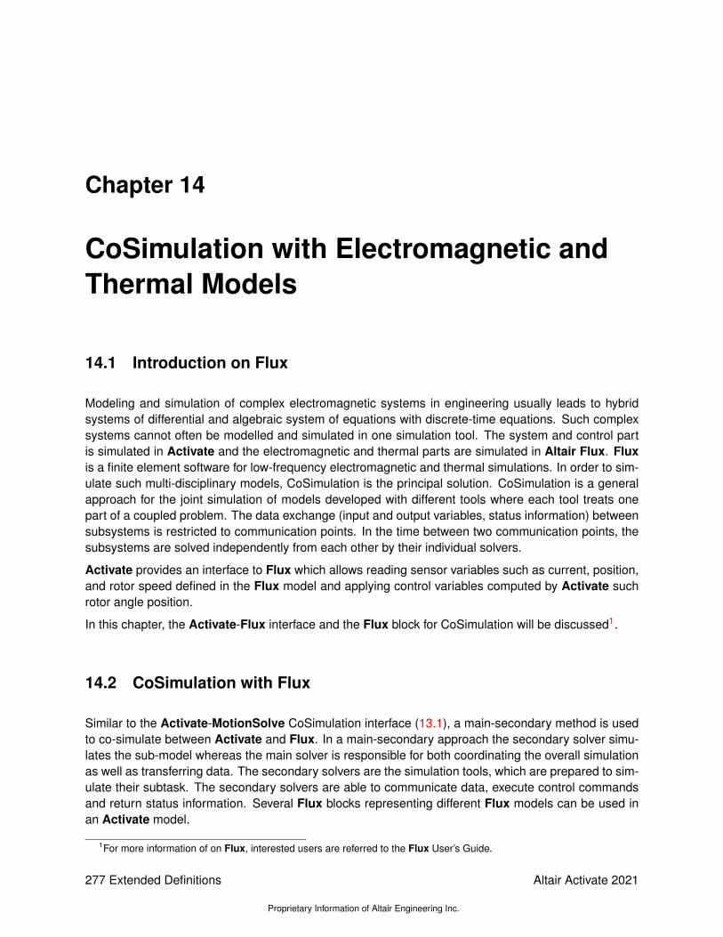
Chapter 14
CoSimulation with Electromagnetic andThermal Models
14.1 Introduction on Flux
Modeling and simulation of complex electromagnetic systems in engineering usually leads to hybridsystems of differential and algebraic system of equations with discrete-time equations. Such complexsystems cannot often be modelled and simulated in one simulation tool. The system and control partis simulated in Activate and the electromagnetic and thermal parts are simulated in Altair Flux. Fluxis a finite element software for low-frequency electromagnetic and thermal simulations. In order to sim-ulate such multi-disciplinary models, CoSimulation is the principal solution. CoSimulation is a generalapproach for the joint simulation of models developed with different tools where each tool treats onepart of a coupled problem. The data exchange (input and output variables, status information) betweensubsystems is restricted to communication points. In the time between two communication points, thesubsystems are solved independently from each other by their individual solvers.
Activate provides an interface to Flux which allows reading sensor variables such as current, position,and rotor speed defined in the Flux model and applying control variables computed by Activate suchrotor angle position.
In this chapter, the Activate-Flux interface and the Flux block for CoSimulation will be discussed1.
14.2 CoSimulation with Flux
Similar to the Activate-MotionSolve CoSimulation interface (13.1), a main-secondary method is usedto co-simulate between Activate and Flux. In a main-secondary approach the secondary solver simu-lates the sub-model whereas the main solver is responsible for both coordinating the overall simulationas well as transferring data. The secondary solvers are the simulation tools, which are prepared to sim-ulate their subtask. The secondary solvers are able to communicate data, execute control commandsand return status information. Several Flux blocks representing different Flux models can be used inan Activate model.
1For more information of on Flux, interested users are referred to the Flux User’s Guide.
277 Extended Definitions
Proprietary Information of Altair Engineering Inc.
Altair Activate 2021

The CoSimulation interface lets the user simulate a complex system that includes one or more electro-magnetic and thermal systems (defined by Flux blocks) and several subsystems modeled with Activateblocks.
In the Activate-Flux interface, Activate is the main solver and Flux is secondary solver. The CoSimula-tion interface has been implemented in a block called Flux which is available in the Activate/CoSimulationpalette, as shown in Figure 14.1.
Figure 14.1: Flux block in Activate.
In order to perform the simulation, it is necessary to have Flux installed on the machine. The installationpath of Flux should be provided to Activate in the Preferences of Activate, as shown in Figure 14.2.
Figure 14.2: Defining the Flux installation path in Activate.
In Flux, once a project is created, the interface variables, i.e., input and output to Activate are defined.Then a CoSimulation interface is exported as an *.f2sta component2. The .f2sta componentcontains the Flux project information including the Flux version, the type of Flux solver, and the nameof input and output ports. The information inside the *.f2sta file is loaded by Activate to setup theCoSimulation.
In order to explain the way a CoSimulation is performed, consider a model composed of two simulatorsas shown in Figure 14.3.
2The reader is referred to the Flux User’s Gide for more details on exporting .f2sta components.
Altair Activate 2021
Proprietary Information of Altair Engineering Inc.
Extended Definitions 278

Figure 14.3: CoSimulation between Activate and Flux.
During the CoSimulation, after instantiation and initialization of the Flux solver, inputs to the Flux modelis provided and the output of the Flux block is requested. Suppose that the output of each part iscomputed with following equations:
YAct = FAct(YFlx)YFlx = GFlx(YAct)
In order to co-simulate this system, this equation should be solved at each communication instant.FAct and GFlx functions are usually complex, non-linear, and time-dependent relationships, as a result,iterative methods are the only choice for solving such equations.
This method has been illustrated in Figure 14.4;
Figure 14.4: CoSimulation method used in Activate.
The Activate simulator is the main solver and advances the time. The following steps for the CoSimu-lation and time synchronization between Activate and Flux is done, as shown in Figure 14.4.
1. The Activate simulator updates the input of the Flux block at instant tn and requests the Fluxoutput at tn.
2. The Flux block reads its inputs and performs either a complete computation or a simple extrapo-lation to compute the output at tn.
3. The Activate simulator advances the time to tn+1 and repeats.
Usually in order to get a correct result, the communication step-size (time between two communicationinstants) should not be larger than the smallest time-constant of secondary solvers. Often smallercommunication step-size results in better convergence but longer simulation time.
The CoSimulation method shown in 14.4 is a rough representation of the CoSimulation method betweenActivate and Flux. There are subtle details about the way Flux block is called during the CoSimulation.Actually, each time the Flux engine performs a computation, the whole finite element computation is
279 Extended Definitions
Proprietary Information of Altair Engineering Inc.
Altair Activate 2021

done in Flux with the recent input received from Activate. But, each Flux engine computation is verycostly in time. Then, it is crucial to reduce the number of computation of Flux to reduce the CoSimulationtime.
In order to reduce the simulation time there are two solutions. The first way is done inside the Fluxengine, i.e., the Flux engine does not perform the computation, if it is not necessary. In fact, a simpleintuitive method to reduce the number of Flux computation is to not performing the computation insideFlux, if input values of the Flux block, provided by Activate have not changed within a range. In thisway, a parameter in the Flux block GUI is used to define the percentage in input variations. The pa-rameter ’Minimal input variation’ specifies the percentage of input variation between two consecutivecalculations of Flux. If the Flux engine performs a computation at time tn, the next Flux engine com-putation at tn+1 will be carried out only if the change in inputs exceeds the designated value. If theFlux engine calculation is not carried out, Flux block outputs are extrapolated based on the ’Outputextrapolation order’ value.
This method is useful when the signal incoming from Activate is almost steady or does not changevery fast with respect to Activate signals. Note that this solution may become troublesome, if theFlux component contains time-dependent elements with fast time constants. Suppose there is a timedependent Flux model whose inputs provided by Activate are Constant values. If the ’Minimal inputvariation’ parameter is specified, since the block inputs does not change during the simulation, theFlux engine will perform the computation only once, which provides incorrect result. Because, sincethe Flux model is time dependent, there is no computation to show the signal variations inside the Fluxcomponent. If a minimum input variation parameter is specified, in order to force the Flux engine toperform a computation, the ’Maximum computation interval’ parameter is used. If this parameteris set to Tm value, the Flux engine performs at least one computation each Tm ± 10% seconds toensure capturing the signal variations inside the Flux component. In order to disable the parameter’Minimal input variation’, zero value or a very high value such as 1000% may be used. The parameter’Maximum computation interval’ is ignored if the parameter ’Minimal input variation’ is not used.As a rule of thumb, the time step-size used by the Flux numerical solver would be a appropriate valuefor this this parameter.
The second way to reduce the simulation time is to reduce the number of calls to the Flux engine. Inorder to advance the time in Activate and take a step, the Activate simulator engine calls blocks inmodel several times for several reasons, e.g., at solver mesh-points, at discrete time-events, at zero-crossing time instants, at internal numerical solver points. At all of these instants, the Flux block isinvoked and its outputs are read by Activate. For some of these invocations, it is useless to invoke theFlux engine to perform a computation and then update the outputs. For example, at internal updatesrequired by the numerical solver, the updated Flux output is not required and an extrapolation of theprevious outputs is sufficient. In the Flux block GUI, the Call Flux at Activate event instants checkboxin the Flux Activation tab 14.3.2 indicates if at discrete event time instants of the Activate simulator,the Flux engine computation is required. By default, the Flux block is invoked only at simulator mesh-points. If this checkbox is checked, the Flux block is called at mesh-points and at all discrete-timeevents of the simulator. If the checkbox is not checked, at discrete-event time instant, the Flux engineperforms an extrapolation and no costly computation is done. Note that even if this extra point checkboxis checked, it does not mean that there will be a Flux computation at a point. Actually, it is the Fluxengine who decides if a computation or an extrapolation should be done, based on the ’Minimal inputvariation’ and ’Maximum computation interval’ values.
It is important to indicate that when the Flux block is externally activated (i.e., External Activation’checkbox is checked), the ’Minimal input variation’ and ’Maximum computation interval’, as well
Altair Activate 2021
Proprietary Information of Altair Engineering Inc.
Extended Definitions 280
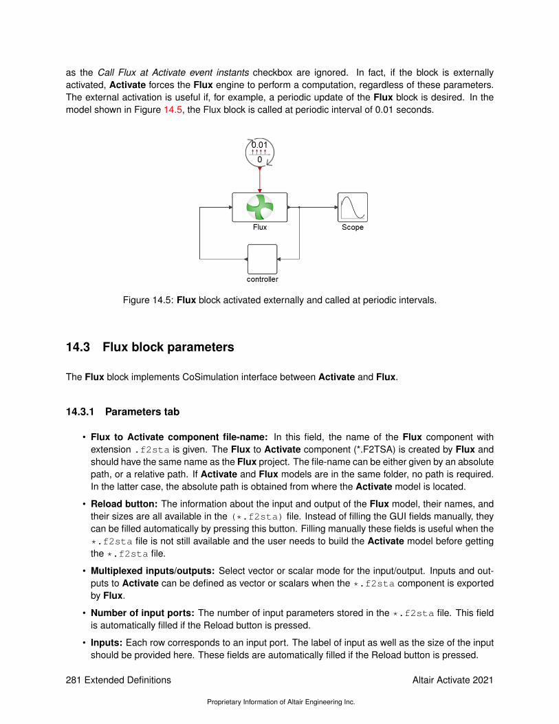
as the Call Flux at Activate event instants checkbox are ignored. In fact, if the block is externallyactivated, Activate forces the Flux engine to perform a computation, regardless of these parameters.The external activation is useful if, for example, a periodic update of the Flux block is desired. In themodel shown in Figure 14.5, the Flux block is called at periodic interval of 0.01 seconds.
Figure 14.5: Flux block activated externally and called at periodic intervals.
14.3 Flux block parameters
The Flux block implements CoSimulation interface between Activate and Flux.
14.3.1 Parameters tab
• Flux to Activate component file-name: In this field, the name of the Flux component withextension .f2sta is given. The Flux to Activate component (*.F2TSA) is created by Flux andshould have the same name as the Flux project. The file-name can be either given by an absolutepath, or a relative path. If Activate and Flux models are in the same folder, no path is required.In the latter case, the absolute path is obtained from where the Activate model is located.
• Reload button: The information about the input and output of the Flux model, their names, andtheir sizes are all available in the (*.f2sta) file. Instead of filling the GUI fields manually, theycan be filled automatically by pressing this button. Filling manually these fields is useful when the*.f2sta file is not still available and the user needs to build the Activate model before gettingthe *.f2sta file.
• Multiplexed inputs/outputs: Select vector or scalar mode for the input/output. Inputs and out-puts to Activate can be defined as vector or scalars when the *.f2sta component is exportedby Flux.
• Number of input ports: The number of input parameters stored in the *.f2sta file. This fieldis automatically filled if the Reload button is pressed.
• Inputs: Each row corresponds to an input port. The label of input as well as the size of the inputshould be provided here. These fields are automatically filled if the Reload button is pressed.
281 Extended Definitions
Proprietary Information of Altair Engineering Inc.
Altair Activate 2021
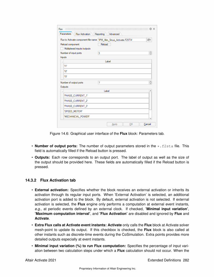
Figure 14.6: Graphical user interface of the Flux block: Parameters tab.
• Number of output ports: The number of output parameters stored in the *.f2sta file. Thisfield is automatically filled if the Reload button is pressed.
• Outputs: Each row corresponds to an output port. The label of output as well as the size ofthe output should be provided here. These fields are automatically filled if the Reload button ispressed.
14.3.2 Flux Activation tab
• External activation: Specifies whether the block receives an external activation or inherits itsactivation through its regular input ports. When ’External Activation’ is selected, an additionalactivation port is added to the block. By default, external activation is not selected. If externalactivation is selected, the Flux engine only performs a computation at external event instants,e.g., at periodic events defined by an external clock. If checked, ’Minimal input variation’,’Maximum computation interval’, and ’Flux Activation’ are disabled and ignored by Flux andActivate.
• Extra Flux calls at Activate event instants: Activate only calls the Flux block at Activate solvermesh-point to update its output. If this checkbox is checked, the Flux block is also called atother instants such as discrete-time events during the CoSimulation. Extra points provides moredetailed outputs especially at event instants.
• Minimal input variation (%) to run Flux computation: Specifies the percentage of input vari-ation between two calculation steps under which a Flux calculation should not occur. When the
Altair Activate 2021
Proprietary Information of Altair Engineering Inc.
Extended Definitions 282

Figure 14.7: Graphical user interface of the Flux block: Flux Activation tab.
Flux calculation is not carried out, outputs are computed based on the ’Output extrapolation or-der’ that is defined, therefore permitting several Activate time steps to be carried out without anyFlux calculations.
• Maximum computation interval: If a non-zero ’Maximum computation interval’ is provided,and a non-zero ’Minimal input variation’ is specified, the Flux engine is forced to perform acomputation not later than the ’Maximum computation interval’ since the last computation,even if the input values have not changed.
• Output extrapolation order: Choose the output extrapolation order (0 : zero-order hold extrap-olation, 1 : linear extrapolation). If ’Minimal input variation’, ’Maximum computation interval’parameters are defined and used, when the Flux engine does not perform the computation, theoutput of the Flux block is provided using extrapolation. In general, if the Flux simulator enginedoes not perform the complete calculation, e.g., when the Activate simulator needs the Fluxoutput at internal solver points (try points), Flux provides the output by extrapolation.
• Add one-step delay: Add a one-step delay to help avoid the algebraic loops caused by the Fluxblock.
14.3.3 Reporting tab
• Subsampling (Reduced result storage): N (which should be greater than 2) means one out ofN data is stored in the result data file in Flux. This feature is available in Flux version 2018 andlater.
283 Extended Definitions
Proprietary Information of Altair Engineering Inc.
Altair Activate 2021

Figure 14.8: Graphical user interface of the Flux block: Report tab.
• Flux console display: Select the check box to turn on the Flux display console, though this maydrastically slow down the computation.
• Log file name (*.log): Activate messages as well as messages communicated from Flux toActivate are logged into this file. ’stderr’ and ’stdout’ are valid values that output log messagesinto the standard output.
14.3.4 Advanced tab
• Current Flux version: Displays the Flux version in use. If the installation path of Flux is specifiedin Preferences of Activate, this field indicates the version of that installation. If no installationpath is specified, the user may specify the Flux installation path by defining the environmentvariable ’INSTALLFLUX’. For example, in the OML command window of Activate, the user canenter: setenv(’INSTALLFLUX’,’D:/AltairSofwtares/Flux-2020/flux/Flux’)
• Flux component version: Flux version used to generate the coupling component, i.e, the*.f2sta file. This information is stored in the *.f2sta file.
• Flux solver: Displays the Flux solver in use. This information is stored in the *.f2sta file.
• Numerical memory (MB): Specifies the memory used for the various modeling actions. 3Dmesh and solving processes (Flux 2D-3D) include a high memory demand. Memory allocationis a function of the application type (real/complex) and matrix size for the solving process. Thedefault value of this information is stored in the *.f2sta file.
Altair Activate 2021
Proprietary Information of Altair Engineering Inc.
Extended Definitions 284

Figure 14.9: Graphical user interface of the Flux block: Advanced tab.
• Character memory (MB): Character memory is used for storing entity names such as parame-ters, transformations, regions, and project names presented in the directory. The default value ofthis information is stored in the *.f2sta file.
• Number of cores: Number of cores used by Flux during CoSimulation. This feature is availablein Flux version 2018 and above. in Flux-2D, only 1 core is used.
14.4 Example: Brushless AC embedded permanent magnet motor
Consider the model in Figure 14.10 which is a model for a brushless AC embedded permanent magnetmotor. The motor is derived by Activate sine wave signals.
The simulation result is shown in Figure 14.11.
14.5 Example: Externally activated block
The Cosimulation with Flux block is usually slow due to numerous calls to the Flux engine. ThisCoSimulation of the example in Figure 14.10 takes about 190 seconds. In order to reduce the calls tothe Flux engine, the Flux block can be activated with an external clock, instead of the Activate numericalsolver. In Figure 14.12, the model in Figure 14.10, is Activated externally by a clock with the period of0.001 seconds. In this model, the Flux block perform a computation every one milli-second.
285 Extended Definitions
Proprietary Information of Altair Engineering Inc.
Altair Activate 2021

Figure 14.10: The brushless AC motor
Now the simulation only takes 60 seconds. The reason is the reduced number of calls to Flux. The onlydrawback of using external activation is a result which is sampled at clock event instants, as shown inFigure 14.13. The sampled result (blue curve) is supoerposed on the result obtained in Figure 14.11(red curve).
Altair Activate 2021
Proprietary Information of Altair Engineering Inc.
Extended Definitions 286

Figure 14.11: The brushless AC motor: Simulation result.
Figure 14.12: The brushless AC motor: externally activated by a clock.
287 Extended Definitions
Proprietary Information of Altair Engineering Inc.
Altair Activate 2021

Figure 14.13: The brushless AC motor: Simulation result.
Altair Activate 2021
Proprietary Information of Altair Engineering Inc.
Extended Definitions 288

Chapter 15
HyperSpice in Altair Activate
15.1 Introduction
This chapter is dedicated to users who want to model and simulate any electronic circuits inside itssystem description. To cover this field, Activate is proposing an environment and a simulator which isbased on the SPICE language. Without being a specialist in electronic, a designer can easily describeand/or get electronic designs in order to simulate them as a black-box.
15.1.1 What is exactly SPICE ?
SPICE (Simulation Program with Integrated Circuit Emphasis) is a software dedicated to simulatinganalog circuits with the highest accuracy. The language used as input of a SPICE simulator is a textualrepresentation of the electronic circuit. The language itself is called the SPICE language. As it is atextual representation, there is no specific needs to define a circuit. Moreover descriptions can beshared easily without any restrictions.
15.1.2 Why using SPICE ?
The first goal of SPICE is to keep the best accuracy for the simulation results. Over the time SPICEbecame a reference by silicon foundries as well as analog circuit designers. Even for digital simulations,timing analysis and power consumptions, SPICE simulation has become essential for building librariesand propose accurate results.
15.2 HyperSpiceTM
HyperSpiceTM is a high performance circuit simulator using SPICE syntax. Its language is based onthe Spice3 spice standard circuit description language. His architecture is based on a hierarchical viewof circuits description and is using a complex elaboration which offers the possibility to simulate hugecircuit providing accuracy and good simulation speed while consuming less memory. HyperSpice isa matrix based simulator. The solving is made by using a specific solver using the latest powerfultechniques of the market for the system resolution.
289 Extended Definitions
Proprietary Information of Altair Engineering Inc.
Altair Activate 2021

HyperSpice is able to perform simulation in three modes:
• DC : Operating point simulation
• Transient: time domain simulation
• AC: frequency response simulation
In terms of device models, HyperSpice is using the Berkeley public models. Devices models level 1, 2and 3 as well as Bsim3 are supported by HyperSpice.
Below is the list of all supported models:
Devices AC/DC and Transient simulationResistor X
Capacitor XInductor X
Mutual inductances XTransmission lines X
Lossy Transmission lines XVsources XIsources X
Voltage Controlled Current Sources XVoltage Controlled Voltage Sources XCurrent Controlled Current Sources XCurrent Controlled Voltage Sources X
Voltage Switches XCurrent Switches X
S-Parameters XDiodes XBJTs XMOSs Level 1, 2, 3 and Bsim 3JFETs Not Supported yet
MESFETs Not supported yet
HyperSpice is taking as input a netlist, written in the Spice syntax. A quick documentation of Spicecomponents is described below, but the user can refer also to the public documentation on
http://bwrcs.eecs.berkeley.edu/Classes/IcBook/SPICE/UserGuide/elements_fr.html
HyperSpice has also been written to be compatible with other Spice simulators such as Spice3, NGspice,LTspice and PSpice as well as some commercial Spice syntax.
15.3 Spice Language
15.3.1 Units
Spice language is defining different symbols associated to different unit factors. These characters canbe used for any setting values. The table below is representing the associated symbols with theirrepresentation:
Altair Activate 2021
Proprietary Information of Altair Engineering Inc.
Extended Definitions 290

V Deg Db f Hz H u k M m n p sVolt Degree Decibel Fento Hertz Henri Micro Kilo Mega Milli Nano Pico Second
15.3.2 Comments
To create a comment in Spice, we can use the symbol ’*’ to set the complete line as comment. Howeverif a partial comment is needed, it is possible to use the symbol ’!’. This symbol means that the commentis starting from the symbol until the end of line. For example:
* This line is a entire comment line
R1 1 0 1k ! This line is a resistor of 1K, but after the ! it is a comment
An important thing to take into account is that the Spice language is considering the first line as acomment. The user should either declare a comment for the first line or consider that the first line willbe ignored.
15.3.3 Resistor
Spice Syntax
RXXXXXXX N1 N2 VALUE
Graphical representation
i
V
N1
N2
RXXXXXXX N1 N2 <VALUE> <MNAME> <L=LENGTH> <W=WIDTH> <TEMP=T>
RLOAD 2 10 10K RMOD 3 7 RMODEL L=10u W=1u
Equation:
V = R ∗ i
Examples:
R1 N1 N2 100
RC1 12 17 1K
N1 and N2 are the two element nodes. VALUE is the resistance (in ohms) and may be positive ornegative but not zero.
291 Extended Definitions
Proprietary Information of Altair Engineering Inc.
Altair Activate 2021
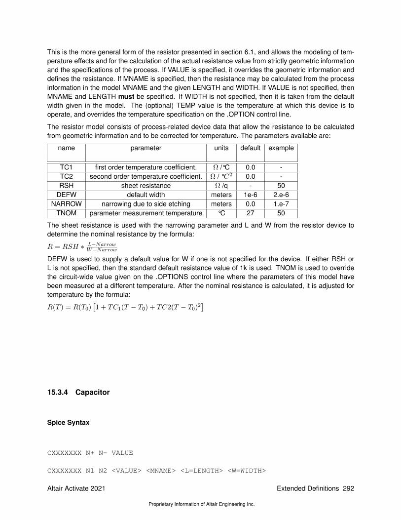
This is the more general form of the resistor presented in section 6.1, and allows the modeling of tem-perature effects and for the calculation of the actual resistance value from strictly geometric informationand the specifications of the process. If VALUE is specified, it overrides the geometric information anddefines the resistance. If MNAME is specified, then the resistance may be calculated from the processinformation in the model MNAME and the given LENGTH and WIDTH. If VALUE is not specified, thenMNAME and LENGTH must be specified. If WIDTH is not specified, then it is taken from the defaultwidth given in the model. The (optional) TEMP value is the temperature at which this device is tooperate, and overrides the temperature specification on the .OPTION control line.
The resistor model consists of process-related device data that allow the resistance to be calculatedfrom geometric information and to be corrected for temperature. The parameters available are:
name parameter units default example
TC1 first order temperature coefficient. Ω /°C 0.0 -TC2 second order temperature coefficient. Ω / °C2 0.0 -RSH sheet resistance Ω /q - 50
DEFW default width meters 1e-6 2.e-6NARROW narrowing due to side etching meters 0.0 1.e-7
TNOM parameter measurement temperature °C 27 50
The sheet resistance is used with the narrowing parameter and L and W from the resistor device todetermine the nominal resistance by the formula:
R = RSH ∗ L−NarrowW−Narrow
DEFW is used to supply a default value for W if one is not specified for the device. If either RSH orL is not specified, then the standard default resistance value of 1k is used. TNOM is used to overridethe circuit-wide value given on the .OPTIONS control line where the parameters of this model havebeen measured at a different temperature. After the nominal resistance is calculated, it is adjusted fortemperature by the formula:
R(T ) = R(T0)[1 + TC1(T − T0) + TC2(T − T0)2
]
15.3.4 Capacitor
Spice Syntax
CXXXXXXX N+ N- VALUE
CXXXXXXX N1 N2 <VALUE> <MNAME> <L=LENGTH> <W=WIDTH>
Altair Activate 2021
Proprietary Information of Altair Engineering Inc.
Extended Definitions 292
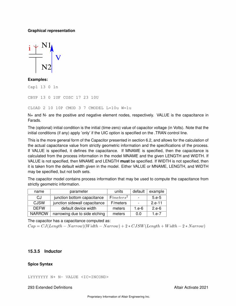
Graphical representation
i
V
N1
N2
Examples:
Cap1 13 0 1n
CBYP 13 0 1UF COSC 17 23 10U
CLOAD 2 10 10P CMOD 3 7 CMODEL L=10u W=1u
N+ and N- are the positive and negative element nodes, respectively. VALUE is the capacitance inFarads.
The (optional) initial condition is the initial (time-zero) value of capacitor voltage (in Volts). Note that theinitial conditions (if any) apply ’only’ if the UIC option is specified on the .TRAN control line.
This is the more general form of the Capacitor presented in section 6.2, and allows for the calculation ofthe actual capacitance value from strictly geometric information and the specifications of the process.If VALUE is specified, it defines the capacitance. If MNAME is specified, then the capacitance iscalculated from the process information in the model MNAME and the given LENGTH and WIDTH. IfVALUE is not specified, then MNAME and LENGTH must be specified. If WIDTH is not specified, thenit is taken from the default width given in the model. Either VALUE or MNAME, LENGTH, and WIDTHmay be specified, but not both sets.
The capacitor model contains process information that may be used to compute the capacitance fromstrictly geometric information.
name parameter units default exampleCJ junction bottom capacitance F/meters2 - 5.e-5
CJSW junction sidewall capacitance F/meters - 2.e-11DEFW default device width meters 1.e-6 2.e-6
NARROW narrowing due to side etching meters 0.0 1.e-7
The capacitor has a capacitance computed as:Cap = CJ(Length−Narrow)(Width−Narrow) + 2 ∗ CJSW (Length+Width− 2 ∗Narrow)
15.3.5 Inductor
Spice Syntax
LYYYYYYY N+ N- VALUE <IC=INCOND>
293 Extended Definitions
Proprietary Information of Altair Engineering Inc.
Altair Activate 2021

Graphical representation
i
V
N1
N2
Examples:
LLINK 42 69 1UH
LSHUNT 23 51 10U IC=15.7MA
N+ and N- are the positive and negative element nodes, respectively. VALUE is the inductance inHenries.
The (optional) initial condition is the initial (time-zero) value of inductor current (in Amps) that flows fromN+, through the inductor, to N-. Note that the initial conditions (if any) apply only if the UIC option isspecified on the .TRAN analysis line.
Equation:
V = Ldidt
15.3.6 Mutual Inductors
Spice syntax
KXXXXXXX LYYYYYYY LZZZZZZZ VALUE
Examples:
K43 LAA LBB 0.999
KXFRMR L1 L2 0.87
The K device is coupled Mutual Inductors. LYYYYYYY and LZZZZZZZ are the names of the two coupledinductors, and VALUE is the coefficient of coupling, K, which must be greater than 0 and less than orequal to 1. Using the ’dot’ convention, place a ’dot’ on the first node of each inductor.
The mutual inductance is equal to:
M =√L& ∗ L2
15.3.7 Mosfet
Spice syntax
MXXXXXXX ND NG NS NB MNAME <L=VAL> <W=VAL> <AD=VAL> <AS=VAL>+ <PD=VAL> <PS=VAL> <NRD=VAL> <NRS=VAL> <OFF>
Altair Activate 2021
Proprietary Information of Altair Engineering Inc.
Extended Definitions 294
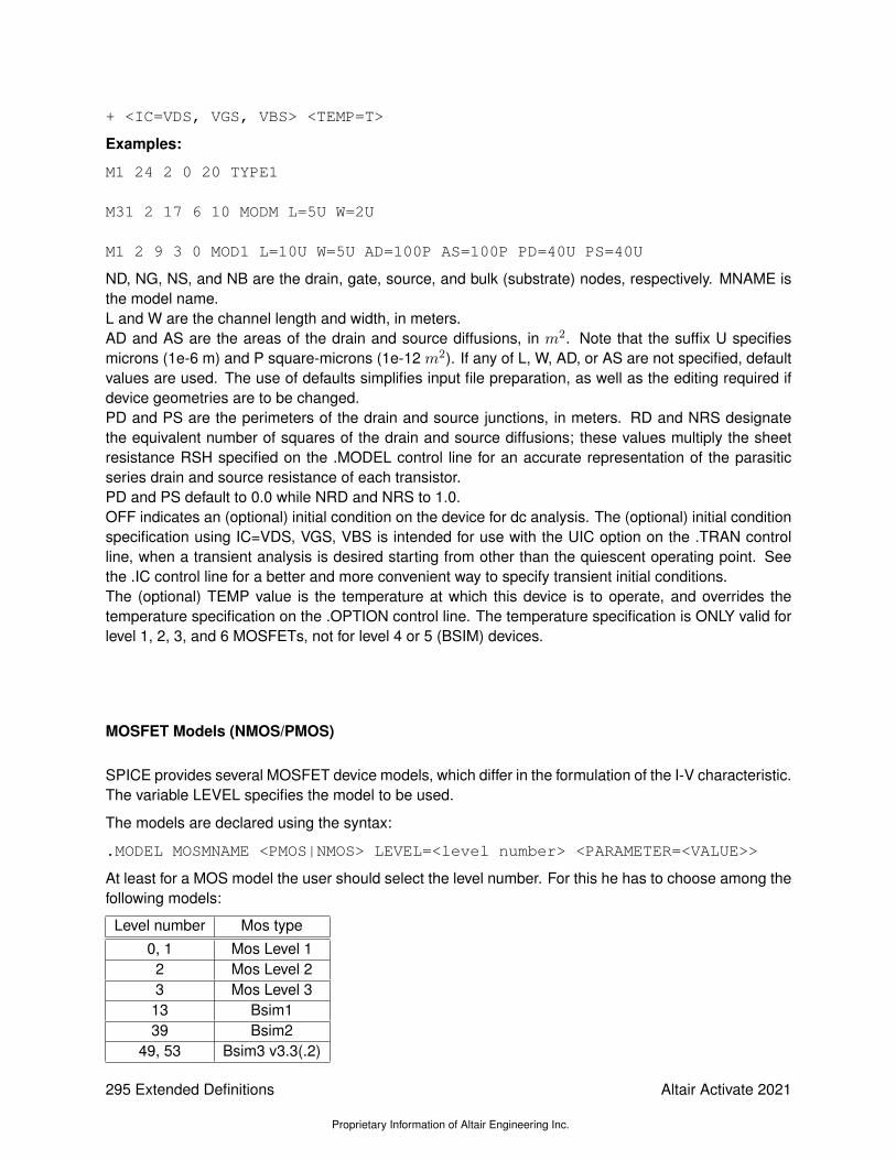
+ <IC=VDS, VGS, VBS> <TEMP=T>
Examples:
M1 24 2 0 20 TYPE1
M31 2 17 6 10 MODM L=5U W=2U
M1 2 9 3 0 MOD1 L=10U W=5U AD=100P AS=100P PD=40U PS=40U
ND, NG, NS, and NB are the drain, gate, source, and bulk (substrate) nodes, respectively. MNAME isthe model name.L and W are the channel length and width, in meters.AD and AS are the areas of the drain and source diffusions, in m2. Note that the suffix U specifiesmicrons (1e-6 m) and P square-microns (1e-12 m2). If any of L, W, AD, or AS are not specified, defaultvalues are used. The use of defaults simplifies input file preparation, as well as the editing required ifdevice geometries are to be changed.PD and PS are the perimeters of the drain and source junctions, in meters. RD and NRS designatethe equivalent number of squares of the drain and source diffusions; these values multiply the sheetresistance RSH specified on the .MODEL control line for an accurate representation of the parasiticseries drain and source resistance of each transistor.PD and PS default to 0.0 while NRD and NRS to 1.0.OFF indicates an (optional) initial condition on the device for dc analysis. The (optional) initial conditionspecification using IC=VDS, VGS, VBS is intended for use with the UIC option on the .TRAN controlline, when a transient analysis is desired starting from other than the quiescent operating point. Seethe .IC control line for a better and more convenient way to specify transient initial conditions.The (optional) TEMP value is the temperature at which this device is to operate, and overrides thetemperature specification on the .OPTION control line. The temperature specification is ONLY valid forlevel 1, 2, 3, and 6 MOSFETs, not for level 4 or 5 (BSIM) devices.
MOSFET Models (NMOS/PMOS)
SPICE provides several MOSFET device models, which differ in the formulation of the I-V characteristic.The variable LEVEL specifies the model to be used.
The models are declared using the syntax:
.MODEL MOSMNAME <PMOS|NMOS> LEVEL=<level number> <PARAMETER=<VALUE>>
At least for a MOS model the user should select the level number. For this he has to choose among thefollowing models:
Level number Mos type0, 1 Mos Level 1
2 Mos Level 23 Mos Level 313 Bsim139 Bsim2
49, 53 Bsim3 v3.3(.2)
295 Extended Definitions
Proprietary Information of Altair Engineering Inc.
Altair Activate 2021

The DC characteristics of the level 1 through level 3 MOSFETs are defined by the device parametersVTO, KP, LAMBDA, PHI and GAMMA. These parameters are computed by SPICE if process parame-ters (NSUB, TOX, ...) are given, but user-specified values always override. VTO is positive (negative) forenhancement mode and negative (positive) for depletion mode N-channel (P-channel) devices. Chargestorage is modeled by three constant capacitors, CGSO, CGDO, and CGBO which represent overlapcapacitances, by the nonlinear thin-oxide capacitance which is distributed among the gate, source,drain, and bulk regions, and by the nonlinear depletion-layer capacitances for both substrate junctionsdivided into bottom and periphery, which vary as the MJ and MJSW power of junction voltage respec-tively, and are determined by the parameters CBD, CBS, CJ, CJSW, MJ, MJSW and PB.Charge storage effects are modeled by the piecewise linear voltages-dependent capacitance modelproposed by Meyer. The thin-oxide charge-storage effects are treated slightly different for the LEVEL=1model. These voltage-dependent capacitances are included only if TOX is specified in the input de-scription and they are represented using Meyer’s formulation.
There is some overlap among the parameters describing the junctions, e.g. the reverse current canbe input either as IS (in A) or as JS (in A/m2). Whereas the first is an absolute value the second ismultiplied by AD and AS to give the reverse current of the drain and source junctions respectively. Thismethodology has been chosen since there is no sense in relating always junction characteristics withAD and AS entered on the device line; the areas can be defaulted. The same idea applies also to thezero-bias junction capacitances CBD and CBS (in F) on one hand, and CJ (in F/m2) on the other. Theparasitic drain and source series resistance can be expressed as either RD and RS (in ohms) or RSH(in Ω/sq.), the latter being multiplied by the number of squares NRD and NRS input on the device line.
SPICE level 1, 2, 3 parameters:
Altair Activate 2021
Proprietary Information of Altair Engineering Inc.
Extended Definitions 296

name parameter units default example1 LEVEL model index - 12 VTO zero-bias threshold voltage (VT0) V 0.0 1.03 KP transconductance parameter A/V 2 2.0e-5 3.1e-54 GAMMA bulk threshold parameter () V 1/2 0.0 0.375 PHI surface potential () V 0.6 0.656 LAMBDA channel-length modulation 1/V 0.0 0.02
MOS1 and MOS2 only7 RD drain ohmic resistance Ω 0.0 1.08 RS source ohmic resistance Ω 0.0 1.09 CBD zero-bias B-D junction capacitance F 0.0 20fF10 CBS zero-bias B-S junction capacitance F 0.0 20fF11 IS bulk junction saturation current (IS) A 1.0e-14 1.0e-1512 PB bulk junction potential V 0.8 0.8713 CGSO gate-source overlap capacitance F/m 0.0 4.0e-11
per meter channel width14 CGDO gate-drain overlap capacitance F/m 0.0 4.0e-11
per meter channel width15 CGBO gate-bulk overlap capacitance F/m 0.0 2.0e-10
per meter channel length16 RSH drain and source diffusion Ω/q 0.0 10.0
sheet resistance17 CJ zero-bias bulk junction bottom cap. F/m2 0.0 2.0e-4
per sq-meter of junction area18 MJ bulk junction bottom grading coeff. - 0.5 0.519 CJSW zero-bias bulk junction sidewall cap. F/m 0.0 1.0e-9
per meter of junction perimeter20 MJSW bulk junction sidewall grading coeff. - 0.50(level1)
0.33(level2,3)21 JS bulk junction saturation current A/m2 1.0e-8
per sq-meter of junction area22 TOX oxide thickness meter 1.0e-7 1.0e-723 NSUB substrate doping 1/cm3 0.0 4.0e1524 NSS surface state density 1/cm2 0.0 1.0e1025 NFS fast surface state density 1/cm2 0.0 1.0e1026 TPG type of gate material: - 1.0
+1 opp. to substrate-1 same as substrate0 Al gate
27 XJ metallurgical junction depth meter 0.0 128 LD lateral diffusion meter 0.0 0.829 UO surface mobility cm2/Vs 600 700
297 Extended Definitions
Proprietary Information of Altair Engineering Inc.
Altair Activate 2021

30 UCRIT critical field for mobility V/cm 1.0e4 1.0e4degradation (MOS2 only)
31 UEXP critical field exponent in - 0.0 0.1mobility degradation (MOS2 only)
32 UTRA transverse field coeff. (mobility) - 0.0 0.3(deleted for MOS2)
33 VMAX maximum drift velocity of carriers m/s 0.0 5.0e434 NEFF total channel-charge (fixed and - 1.0 5.0
mobile) coefficient (MOS2 only)35 KF flicker noise coefficient - 0.0 1.0e-2636 AF flicker noise exponent - 1.0 1.237 FC coefficient for forward-bias - 0.5
depletion capacitance formula38 DELTA width effect on threshold voltage - 0.0 1.0
(MOS2 and MOS3)39 THETA mobility modulation (MOS3 only) 1/V 0.0 0.140 ETA static feedback (MOS3 only) - 0.0 1.041 KAPPA saturation field factor (MOS3 only) - 0.2 0.542 TNOM parameter measurement temperature C 27 50
For more information on models see the Berkeley device models documentation.
15.3.8 BJT
Spice syntax
QXXXXXXX NC NB NE <NS> MNAME <AREA> <OFF> <IC=VBE, VCE> <TEMP=T>
.MODEL MNAME NPN|PNP <Param=Value>
Examples:
Q23 10 24 13 QMOD IC=0.6
Q50A 11 26 4 20 MOD1
The BJT device is a Bipolar Junction Transistor.
NC, NB, and NE are the collector, base, and emitter nodes, respectively.NS is the (optional) substrate node. If unspecified, ground is used.MNAME is the model name, AREA is the area factor, and OFF indicates an (optional) initial conditionon the device for the dc analysis. If the area factor is omitted, a value of 1.0 is assumed.The (optional) initial condition specification using IC=VBE, VCE is intended for use with the UIC optionon the .TRAN control line, when a transient analysis is desired starting from other than the quiescentoperating point. See the .IC control line description for a better way to set transient initial conditions.The (optional) TEMP value is the temperature at which this device is to operate, and overrides thetemperature specification on the .OPTION control line.
Altair Activate 2021
Proprietary Information of Altair Engineering Inc.
Extended Definitions 298
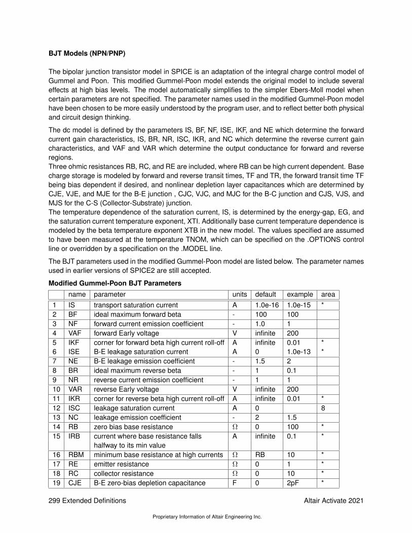
BJT Models (NPN/PNP)
The bipolar junction transistor model in SPICE is an adaptation of the integral charge control model ofGummel and Poon. This modified Gummel-Poon model extends the original model to include severaleffects at high bias levels. The model automatically simplifies to the simpler Ebers-Moll model whencertain parameters are not specified. The parameter names used in the modified Gummel-Poon modelhave been chosen to be more easily understood by the program user, and to reflect better both physicaland circuit design thinking.
The dc model is defined by the parameters IS, BF, NF, ISE, IKF, and NE which determine the forwardcurrent gain characteristics, IS, BR, NR, ISC, IKR, and NC which determine the reverse current gaincharacteristics, and VAF and VAR which determine the output conductance for forward and reverseregions.Three ohmic resistances RB, RC, and RE are included, where RB can be high current dependent. Basecharge storage is modeled by forward and reverse transit times, TF and TR, the forward transit time TFbeing bias dependent if desired, and nonlinear depletion layer capacitances which are determined byCJE, VJE, and MJE for the B-E junction , CJC, VJC, and MJC for the B-C junction and CJS, VJS, andMJS for the C-S (Collector-Substrate) junction.The temperature dependence of the saturation current, IS, is determined by the energy-gap, EG, andthe saturation current temperature exponent, XTI. Additionally base current temperature dependence ismodeled by the beta temperature exponent XTB in the new model. The values specified are assumedto have been measured at the temperature TNOM, which can be specified on the .OPTIONS controlline or overridden by a specification on the .MODEL line.
The BJT parameters used in the modified Gummel-Poon model are listed below. The parameter namesused in earlier versions of SPICE2 are still accepted.
Modified Gummel-Poon BJT Parameters
name parameter units default example area1 IS transport saturation current A 1.0e-16 1.0e-15 *2 BF ideal maximum forward beta - 100 1003 NF forward current emission coefficient - 1.0 14 VAF forward Early voltage V infinite 2005 IKF corner for forward beta high current roll-off A infinite 0.01 *6 ISE B-E leakage saturation current A 0 1.0e-13 *7 NE B-E leakage emission coefficient - 1.5 28 BR ideal maximum reverse beta - 1 0.19 NR reverse current emission coefficient - 1 110 VAR reverse Early voltage V infinite 20011 IKR corner for reverse beta high current roll-off A infinite 0.01 *12 ISC leakage saturation current A 0 813 NC leakage emission coefficient - 2 1.514 RB zero bias base resistance Ω 0 100 *15 IRB current where base resistance falls A infinite 0.1 *
halfway to its min value16 RBM minimum base resistance at high currents Ω RB 10 *17 RE emitter resistance Ω 0 1 *18 RC collector resistance Ω 0 10 *19 CJE B-E zero-bias depletion capacitance F 0 2pF *
299 Extended Definitions
Proprietary Information of Altair Engineering Inc.
Altair Activate 2021

20 VJE B-E built-in potential V 0.75 0.621 MJE B-E junction exponential factor - 0.33 0.3322 TF ideal forward transit time sec 0 0.1ns23 XTF coefficient for bias dependence of TF - 024 VTF voltage describing VBC V infinite
dependence of TF25 ITF high-current parameter A 0 *
for effect on TF26 PTF excess phase at freq=1.0/(TF*2PI) Hz deg 027 CJC B-C zero-bias depletion capacitance F 0 2pF *28 VJC B-C built-in potential V 0.75 0.529 MJC B-C junction exponential factor - 0.33 0.530 XCJC fraction of B-C depletion capacitance - 1
connected to internal base node31 TR ideal reverse transit time sec 0 10ns32 CJS zero-bias collector-substrate capacitance F 0 2pF *33 VJS substrate junction built-in potential V 0.7534 MJS substrate junction exponential factor - 0 0.535 XTB forward and reverse beta - 0
temperature exponent36 EG energy gap for temperature eV 1.11
effect on IS37 XTI temperature exponent for effect on IS - 338 KF flicker-noise coefficient - 039 AF flicker-noise exponent - 140 FC coefficient for forward-bias - 0.5
depletion capacitance formula41 TNOM Parameter measurement temperature °C 27 50
15.3.9 JFET
Spice Syntax
JXXXXXXX ND NG NS MNAME <AREA> <OFF> <IC=VDS, VGS> <TEMP>
Examples:
J1 7 2 3 JM1 OFF
The JFET device is a Junction Field-Effect Transistors (JFETs). ND, NG, and NS are the drain, gate, andsource nodes, respectively. MNAME is the model name, AREA is the area factor, and OFF indicatesan (optional) initial condition on the device for dc analysis. If the area factor is omitted, a value of 1.0 isassumed.
The (optional) initial condition specification, using IC=VDS, VGS is intended for use with the UIC optionon the .TRAN control line, when a transient analysis is desired starting from other than the quiescentoperating point. See the .IC control line for a better way to set initial conditions.
The (optional) TEMP value is the temperature at which this device is to operate, and overrides the
Altair Activate 2021
Proprietary Information of Altair Engineering Inc.
Extended Definitions 300

temperature specification on the .OPTION control line.
JFET Models (NJF/PJF)
The JFET model is derived from the FET model of Shichman and Hodges. The dc characteristics aredefined by the parameters VTO and BETA, which determine the variation of drain current with gatevoltage, LAMBDA, which determines the output conductance, and IS, the saturation current of the twogate junctions. Two ohmic resistances, RD and RS, are included. Charge storage is modeled bynonlinear depletion layer capacitances for both gate junctions which vary as the -1/2 power of junctionvoltage and are defined by the parameters CGS, CGD, and PB.
Note that in Spice3f and later, a fitting parameter B has been added. For details, see [9].
name parameter units default example area1 VTO threshold voltage (VT0) V -2.0 -2.02 BETA transconductance parameter A/V 2 1.0e-4 1.0e-3 *3 LAMBDA channel-length modulation 1/V 0 1.0e-44 RD drain ohmic resistance Ω 0 100 *5 RS source ohmic resistance Ω 0 100 *6 CGS zero-bias G-S junction capacitance (Cgs) F 0 5pF *7 CGD zero-bias G-D junction capacitance (Cgs) F 0 1pF *8 PB gate junction potential V 1 0.69 IS gate junction saturation current (IS) A 1.0e-14 1.0e-14 *10 B doping tail parameter - 1 1.111 KF flicker noise coefficient - 012 AF flicker noise exponent - 113 FC coefficient for forward-bias - 0.514 TNOM parameter measurement temperature °C 27 50
15.3.10 Switches
V-Switch
Spice syntax
SXXXXXXX N+ N- NC+ NC- MODEL <ON><OFF>
Examples:
.MODEL smodel1 RON=100K
Switch1 1 2 10 0 smodel1
The S- device is an ideal voltage switch. Nodes 1 and 2 are the nodes between which the switchterminals are connected. The model name is mandatory while the initial conditions are optional nodes,3 and 4 are the positive and negative controlling nodes respectively.
301 Extended Definitions
Proprietary Information of Altair Engineering Inc.
Altair Activate 2021

Switch Model (SW)
The switch model allows an almost ideal switch to be described in SPICE.
The switch is not quite ideal, in that the resistance cannot change from 0 to infinity, but must alwayshave a finite positive value. By proper selection of the on and off resistances, they can be effectivelyzero and infinity in comparison to other circuit elements.
The parameters available are:name parameter units defaultVT threshold voltage Volts 0.0VH hysteresis voltage Volts 0.0RON on resistance 1.0ROFF off resistance 1/GMIN*
*(See the .OPTIONS control line for a description of GMIN, its default value results in an off-resistanceof 1.0e+12 ohms.)
The use of an ideal element that is highly nonlinear such as a switch can cause large discontinuities tooccur in the circuit node voltages.
A rapid change such as that associated with a switch changing state can cause numerical roundoff ortolerance problems leading to erroneous results or timestep difficulties.
The user of switches can improve the situation by taking the following steps:
First, it is wise to set ideal switch impedances just high or low enough to be negligible with respect toother circuit elements. Using switch impedances that are close to “ideal” in all cases aggravates theproblem of discontinuities mentioned above. Of course, when modeling real devices such as MOS-FETS, the on resistance should be adjusted to a realistic level depending on the size of the devicebeing modeled.
If a wide range of ON to OFF resistance must be used in the switches (ROFF/RON >1e+12), thenthe tolerance on errors allowed during transient analysis should be decreased by using the .OPTIONScontrol line and specifying TRTOL to be less than the default value of 7.0. When switches are placedaround capacitors, then the option CHGTOL should also be reduced. Suggested values for these twooptions are 1.0 and 1e-16 respectively. These changes inform SPICE3 to be more careful around theswitch points so that no errors are made due to the rapid change in the circuit.
C-Switch
Spice syntax
WYYYYYYY N+ N- VNAM MODEL <ON><OFF>
Examples:
.MODEL switchmod1 IT=1e-3
W1 1 2 vclock switchmod1
The W-device is a Current controlled switch. Nodes 1 and 2 are the nodes between which the switchterminals are connected. The model name is mandatory while the initial conditions are optional. Thecontrolling current is that through the specified voltage source. The direction of positive controlling
Altair Activate 2021
Proprietary Information of Altair Engineering Inc.
Extended Definitions 302

current flow is from the positive node, through the source, to the negative node.
Switch Model (CSW)
The switch model allows an almost ideal switch to be described in SPICE.
The switch is not quite ideal, in that the resistance cannot change from 0 to infinity, but must alwayshave a finite positive value. By proper selection of the on and off resistances, they can be effectivelyzero and infinity in comparison to other circuit elements.
The parameters available are:name parameter units defaultIT threshold current Amps 0.0IH hysteresis current Amps 0.0RON on resistance 1.0ROFF off resistance 1/GMIN*
*(See the .OPTIONS control line for a description of GMIN, its default value results in an off-resistanceof 1.0e+12 ohms.)
The use of an ideal element that is highly nonlinear such as a switch can cause large discontinuities tooccur in the circuit node voltages. A rapid change such as that associated with a switch changing statecan cause numerical roundoff or tolerance problems leading to erroneous results or timestep difficulties.The user of switches can improve the situation by taking the following steps:
First, it is wise to set ideal switch impedances just high or low enough to be negligible with respect toother circuit elements. Using switch impedances that are close to “ideal” in all cases aggravates theproblem of discontinuities mentioned above. Of course, when modeling real devices such as MOS-FETS, the on resistance should be adjusted to a realistic level depending on the size of the devicebeing modeled.
If a wide range of ON to OFF resistance must be used in the switches (ROFF/RON >1e+12), thenthe tolerance on errors allowed during transient analysis should be decreased by using the .OPTIONScontrol line and specifying TRTOL to be less than the default value of 7.0. When switches are placedaround capacitors, then the option CHGTOL should also be reduced. Suggested values for these twooptions are 1.0 and 1e-16 respectively. These changes inform SPICE3 to be more careful around theswitch points so that no errors are made due to the rapid change in the circuit.
15.3.11 Transmission Lines
Lossless Transmission Lines
Spice syntax
TXXXXXXX N1 N2 N3 N4 Z0=VALUE <TD=VALUE> <F=FREQ <NL=NRMLEN>>+ <IC=V1, I1, V2, I2>
Examples:
T1 1 0 2 0 Z0=50 TD=10NS
The T device is a Lossless Transmission Lines.
303 Extended Definitions
Proprietary Information of Altair Engineering Inc.
Altair Activate 2021

N1 and N2 are the nodes at port 1.
N3 and N4 are the nodes at port 2.
Z0 is the characteristic impedance.
The length of the line may be expressed in either of two forms. The transmission delay, TD, may bespecified directly (as TD=10ns, for example). Alternatively, a frequency F may be given, together withNL, the normalized electrical length of the transmission line with respect to the wavelength in the lineat the frequency F. If a frequency is specified but NL is omitted, 0.25 is assumed (that is, the frequencyis assumed to be the quarter-wave frequency). Note that although both forms for expressing the linelength are indicated as optional, one of the two must be specified.
Note that this element models only one propagating mode. If all four nodes are distinct in the actualcircuit, then two modes may be excited. To simulate such a situation, two transmission-line elementsare required.
The (optional) initial condition specification consists of the voltage and current at each of the transmis-sion line ports. Note that the initial conditions (if any) apply ’only’ if the UIC option is specified on the.TRAN control line.
Note that a lossy transmission line (see below) with zero loss may be more accurate than than thelossless transmission line due to implementation details.
Lossy Transmission Lines
Spice syntax
OXXXXXXX N1 N2 N3 N4 MNAME
Examples:
O23 1 0 2 0 LOSSYMOD
OCONNECT 10 5 20 5 INTERCONNECT
The O device is a Lossy Transmission Lines. This is a two-port convolution model for single-conductorlossy transmission lines.
N1 and N2 are the nodes at port 1
N3 and N4 are the nodes at port 2.
Note that a lossy transmission line with zero loss may be more accurate than the lossless transmissionline due to implementation details.
Lossy Transmission Line Model (LTRA)
The uniform RLC/RC/LC/RG transmission line model (referred to as the LTRA model henceforth) mod-els a uniform constant-parameter distributed transmission line.
The RC and LC cases may also be modeled using the URC and TRA models. However, the newerLTRA model is usually faster and more accurate than the others.
The operation of the LTRA model is based on the convolution of the transmission line’s impulse re-
Altair Activate 2021
Proprietary Information of Altair Engineering Inc.
Extended Definitions 304

sponses with its inputs.
The LTRA model takes a number of parameters, some of which must be given and some of which areoptional.
name parameter units/type default exampleR resistance/length 0.0 0.2L inductance/length henrys/unit 0.0 9.13e-9G conductance/length mhos/unit 0.0 0.0C capacitance/length farads/unit 0.0 3.65e-12LEN length of line no default 1.0REL breakpoint control arbitrary unit 1 0.5ABS breakpoint control 1 5NOSTEPLIMIT don’t limit timestep to less than flag not set set
line delayNOCONTROL don’t do complex timestep control flag not set setLININTERP use linear interpolation flag not set setMIXEDINTERP use linear when quadratic seems bad not set setCOMPACTREL special reltol for history compaction flag RELTOL 1.0e-3COMPACTABS special abstol for history compaction ABSTOL 1.0e-9TRUNCNR use Newton-Raphson method for flag not set set
timestep controlTRUNCDONTCUT don’t limit timestep to keep flag not set set
impulse-esponse errors low
The following types of lines have been implemented so far:
RLC (uniform transmission line with series loss only), RC (uniform RC line), LC (lossless transmissionline), and RG (distributed series resistance and parallel conductance only).
Any other combination will yield erroneous results and should not be tried.
The length LEN of the line must be specified.
NOSTEPLIMIT is a flag that will remove the default restriction of limiting time-steps to less than the linedelay in the RLC case.
NOCONTROL is a flag that prevents the default limiting of the time-step based on convolution errorcriteria in the RLC and RC cases. This speeds up simulation but may in some cases reduce theaccuracy of results.
LININTERP is a flag that, when specified, will use linear interpolation instead of the default quadraticinterpolation for calculating delayed signals.
MIXEDINTERP is a flag that, when specified, uses a metric for judging whether quadratic interpolationis not applicable and if so uses linear interpolation; otherwise it uses the default quadratic interpolation.
TRUNCDONTCUT is a flag that removes the default cutting of the time-step to limit errors in the actualcalculation of impulse-response related quantities.
COMPACTREL and COMPACTABS are quantities that control the compaction of the past history ofvalues stored for convolution. Larger values of these lower accuracy but usually increase simulationspeed. These are to be used with the TRYTOCOMPACT option, described in the .OPTIONS section.
305 Extended Definitions
Proprietary Information of Altair Engineering Inc.
Altair Activate 2021

TRUNCNR is a flag that turns on the use of Newton-Raphson iterations to determine an appropriatetimestep in the timestep control routines. The default is a trial and error procedure by cutting theprevious timestep in half.
REL and ABS are quantities that control the setting of breakpoints.
The option most worth experimenting with for increasing the speed of simulation is REL. The defaultvalue of 1 is usually safe from the point of view of accuracy but occasionally increases computation time.A value greater than 2 eliminates all breakpoints and may be worth trying depending on the nature of therest of the circuit, keeping in mind that it might not be safe from the viewpoint of accuracy. Breakpointsmay usually be entirely eliminated if it is expected the circuit will not display sharp discontinuities. Valuesbetween 0 and 1 are usually not required but may be used for setting many breakpoints.
COMPACTREL may also be experimented with when the option TRYTOCOMPACT is specified in a.OPTIONS card. The legal range is between 0 and 1. Larger values usually decrease the accuracy ofthe simulation but in some cases improve speed. If TRYTOCOMPACT is not specified on a .OPTIONScard, history compaction is not attempted and accuracy is high.
NOCONTROL, TRUNCDONTCUT and NOSTEPLIMIT also tend to increase speed at the expense ofaccuracy.
15.3.12 Diode
Spice syntax
.MODEL MNAME DIO <Param=value>
DXXXXXXX N1 N2 MNAME <AREA>> <OFF> <IC=VD> <TEMP>
Graphical representation
i
V
N1
N2
Examples:
DBRIDGE 2 10 DIODE1
DCLMP 3 7 DMOD 3.0 IC=0.2
The D device is a junction diode. N1 and N2 are the positive and negative nodes, respectively. N1 isthe Anode and N2 is the Cathode.
MNAME is the model name, AREA is the area factor, and OFF indicates an (optional) starting conditionon the device for dc analysis. If the area factor is omitted, a value of 1.0 is assumed.
The (optional) initial condition specification using IC=VD is intended for use with the UIC option on the
Altair Activate 2021
Proprietary Information of Altair Engineering Inc.
Extended Definitions 306

.TRAN control line, when a transient analysis is desired starting from other than the quiescent operatingpoint.
The (optional) TEMP value is the temperature at which this device is to operate, and overrides thetemperature specification on the .OPTION control line.
Diode Model (D)
The DC characteristics of the diode are determined by the parameters IS and N. An ohmic resistance,RS, is included. Charge storage effects are modeled by a transit time, TT, and a nonlinear depletionlayer capacitance which is determined by the parameters CJO, VJ, and M. The temperature depen-dence of the saturation current is defined by the parameters EG, the energy and XTI, the saturationcurrent temperature exponent.
The nominal temperature at which these parameters were measured is TNOM, which defaults to thecircuit-wide value specified on the .OPTIONS control line. Reverse breakdown is modeled by an expo-nential increase in the reverse diode current and is determined by the parameters BV and IBV (both ofwhich are positive numbers).
name parameter units default example area1 IS saturation current A 1.0e-14 1.0e-14 *2 RS ohmic resistance Ω 0 10 *3 N emission coefficient - 1 1.04 TT transit-time sec 0 0.1ns5 CJO zero-bias junction capacitance F 0 2pF *6 VJ junction potential V 1 0.67 M grading coefficient - 0.5 0.58 EG activation energy eV 1.11 1.11 Si
0.69 Sbd0.67Ge
9 XTI saturation-current temp. exp - 3.0 3.0jn2.0Sbd
10 KF flicker noise coefficient - 011 AF flicker noise exponent - 112 FC coefficient for forward-bias - 0.5
depletion capacitance formula13 BV reverse breakdown voltage V infinite 40.014 IBV current at breakdown voltage A 1.0e-315 TNOM parameter measurement temperature °C 27 50
15.3.13 S-Parameter blocks
Spice syntax
.MODEL MNAME SPARAM <PARAM=VALUE>
YXXXXXX MNAME PARAM: PARAM=VALUE PIN: PIN1 PIN2 .. PINn
307 Extended Definitions
Proprietary Information of Altair Engineering Inc.
Altair Activate 2021

Examples:
.model SPARAMM SPARAM
ysparam SPARAMM param:+ force_passivity=1+ sparamfile=lowpassfilter2.s2p+ pin:+ 2 0 3 0
Graphical representation
a1
b1
b2
a2
S11 = b1a1 |a2=0 S12 = b1
a2 |a1=0
S21 = b2a1 |a2=0 S22 = b2
a2 |a1=0[b1b2
]=
[S11 S12S21 S22
] [a1a2
]A Yelem device which is declared with a model named SPARAM is called an S-Parameter block.
Param name iValueIM LC (Linear Cartesian)
LC (Linear Cartesian)VF (Vector fitting)CS (Cubic spline)
CSL(Cubic Spline Log)EX 1 (Activate) or 0 (Disactivate)
SPARAMFILE Filename of the SnP S-Parameter dataFORCE_PASSIVITY 1(Activate or 0 (Disactivate)
15.3.14 Linear Dependent Sources
Voltage-Controlled Voltage Sources (Esrc)
Spice syntax
EXXXXXXX N+ N- NC+ NC- VALUE
Examples:
E1 2 3 14 1 2.0
N+ is the positive node, and N- is the negative node. NC+ and NC- are the positive and negativecontrolling nodes, respectively. VALUE is the voltage gain.
Altair Activate 2021
Proprietary Information of Altair Engineering Inc.
Extended Definitions 308
Current-Controlled Current Sources (Fsrc)
Spice syntax
FXXXXXXX N+ N- VNAM VALUE
Examples:
F1 13 5 VSENS 5
N+ and N- are the positive and negative nodes, respectively. Current flow is from the positive node,through the source, to the negative node. VNAM is the name of a voltage source through which thecontrolling current flows. The direction of positive controlling current flow is from the positive node,through the source, to the negative node of VNAM. VALUE is the current gain.
Voltage-Controlled Current Sources (Gsrc)
Spice syntax
GXXXXXXX N+ N- NC+ NC- VALUE
Examples:
G1 2 0 5 0 0.1MMHO
N+ and N- are the positive and negative nodes, respectively. Current flow is from the positive node,through the source, to the negative node. NC+ and NC- are the positive and negative controlling nodes,respectively. VALUE is the transconductance (in mhos).
Current-Controlled Voltage Sources (Hsrc)
Spice syntax
HXXXXXXX N+ N- VNAM VALUE
Examples:
HX 5 17 VZ 0.5K
N+ and N- are the positive and negative nodes, respectively. VNAM is the name of a voltage sourcethrough which the controlling current flows. The direction of positive controlling current flow is from thepositive node, through the source, to the negative node of VNAM. VALUE is the transresistance (inohms).
15.3.15 Linear Independent Sources
Voltage Sources
Spice Syntax
VXXXXXXX N+ N- <DC >DC/TRAN Value> <AC <AC Mag < AC Phase>>>
Examples:
309 Extended Definitions
Proprietary Information of Altair Engineering Inc.
Altair Activate 2021

VCC 10 0 DC 6
VIN 13 2 0.001 AC 1 SIN(0 1 1MEG)
VIN 2 0 PWL 0 0 10n 0 11n 3.3 25n 3.3 26n 0 R
N+ and N- are the positive and negative nodes, respectively. Note that voltage sources need not begrounded.
Voltage sources, being used for circuit excitation, are the ’ammeters’ for SPICE, that is, zero valuedvoltage sources may be inserted into the circuit for the purpose of measuring current. They of coursehave no effect on circuit operation since they represent short-circuits.
DC/TRAN is the dc and transient analysis value of the source. If the source value is zero both for dcand transient analyses, this value may be omitted. If the source value is time-invariant (e.g., a powersupply), then the value may optionally be preceded by the letters DC.
ACMAG is the ac magnitude and ACPHASE is the ac phase. The source is set to this value in the acanalysis. If ACMAG is omitted following the keyword AC, a value of unity is assumed. If ACPHASE isomitted, a value of zero is assumed. If the source is not an ac small-signal input, the keyword AC andthe ac values are omitted.
Any independent source can be assigned a time-dependent value for transient analysis. If a source isassigned a time-dependent value, the time-zero value is used for dc analysis.
Pulse
PULSE(V1 V2 TD TR TF PW PER)
V1
V2
Rt PtTd
Pe
Ft
Examples:
VIN 3 0 PULSE(-1 1 2NS 2NS 2NS 50NS 100NS)
parameter default value unitsV1 (initial value) - Volts or AmpsV2 (pulsed value) - Volts or AmpsTD (delay time) 0.0 secondsTR (rise time) TSTEP secondsTF (fall time) TSTEP secondsPW (pulse width) TSTOP secondsPER(period) TSTOP seconds
A single pulse so specified is described by the following table:
Altair Activate 2021
Proprietary Information of Altair Engineering Inc.
Extended Definitions 310

time value0 V1TD V1TD+TR V2TD+TR+PW V2TD+TR+PW V2 V1TSTOP V1
Intermediate points are determined by linear interpolation.
Sinusoidal
SIN(VO VA FREQ TD THETA)
Examples:
VIN 3 0 SIN(0 1 100MEG 1NS 1E10)
parameters default value unitsVO (offset) Volts or AmpsVA (amplitude) Volts or AmpsFREQ (frequency) 1/TSTOP HzTD (delay) 0.0 secondsTHETA (damping factor) 0.0 1/seconds
The shape of the waveform is described by:
time value0 to TD V0
TD to TSTOP V 0 + V A exp−(t−TD)THETA sin(2π ∗ Freq(t+ TD))
Exponential
EXP(V1 V2 TD1 TAU1 TD2 TAU2)
V1
V2
Tau1TD1 TD2 Tau2
Examples:
VIN 3 0 EXP(-4 -1 2NS 30NS 60NS 40NS)
311 Extended Definitions
Proprietary Information of Altair Engineering Inc.
Altair Activate 2021

parameter default value unitsV1 (initial value) - Volts or AmpsV2 (pulsed value) - Volts or AmpsTD1 (rise delay time) 0.0 secondsTAU1 (rise time constant) TSTEP secondsTD2 (fall delay time) TD1+TSTEP secondsTAU2 (fall time TSTEP seconds
The shape of the waveform is described by the following table:
time value0 to TD1 V1
TD1 to TD2 V 1 + (V 2− V 1)[1− exp−(t−TD1)Tau1 ]
TD2 to Tstop V 1 + (V 2− V 1)[1− exp−(t−TD1)Tau1 ] + (V 1− V 2)[1− exp
−(t−TD2)Tau2 ]
Piece-Wise Linear
PWL(T1 V1 <T2; V2 T3 V3 T4 V4 ...>)
V1
V2
V5
V6
V7
t2 t3 t4 t5 t6 t70 t1
V0
V3
V4
Examples:
VCLOCK 7 5 PWL(0 -7 10NS -7 11NS -3 17NS -3 18NS -7 50NS -7)
Each pair of values (Ti, Vi) specifies that the value of the source is Vi (in Volts or Amps) at time=Ti.The value of the source at intermediate values of time is determined by using linear interpolation on theinput values.
Pattern Function
PATTERN VHI VLO < TDELAY TRISE TFALL TSAMPLE BITS R >
Examples:
VPATTERN 1 0 PATTERN 5 0 0 10p 10p 5n 0 1 1 R
Generating a digital like source. The VHI/VHO are used to select the voltages of the digit and thepattern is used for representing the signal.
Current Sources
Spice Syntax
IYYYYYYY N+ N- <<DC <DC/TRAN Value>> <AC <AC Mag <AC Phase>>>
Examples:
Altair Activate 2021
Proprietary Information of Altair Engineering Inc.
Extended Definitions 312

ISRC 1 0 1m
N+ and N- are the positive and negative nodes, respectively. Positive current is assumed to flow fromthe positive node, through the source, to the negative node. A current source of positive value forcescurrent to flow out of the N+ node, through the source, and into the N- node.
DC/TRAN is the dc and transient analysis value of the source. If the source value is zero both for dcand transient analyses, this value may be omitted. If the source value is time-invariant (e.g., a powersupply), then the value may optionally be preceded by the letters DC.
ACMAG is the ac magnitude and ACPHASE is the ac phase. The source is set to this value in the acanalysis. If ACMAG is omitted following the keyword AC, a value of unity is assumed. If ACPHASE isomitted, a value of zero is assumed. If the source is not an ac small-signal input, the keyword AC andthe ac values are omitted.
15.3.16 Hierarchy declaration
Block sub-circuit declaration
In Spice a block can be defined by using the keyword .SUBCKT to define a block or a black box. Thesyntax of the declaration is as follows:
.SUBCKT BNAME PIN1 PIN2 ... PINn <Param1=value> .. <Paramn=value>
* Circuit Description of the subckt *.ENDS
Between these two keywords (.SUBCKT and .ENDS), the user can define any devices, instances orredefine again new blocks.
For example, an inverter can be declared as :
.SUBCKT INVERTER IN OUT VDD GND
.MODEL TN NMOS level=3
.MODEL TP PMOS level=3
* MOS instantiation D G S Bm1 OUT IN GND GND TN w=0.25u l=0.25um2 OUT IN VDD VDD TP w=0.250u l=0.25u.ENDS
Optional parameters can be declared to set some parameters which are considered as new parametersfor the scope of the block.
If a parameter MYPAR=1 is declared on the block definition, it means that inside the block MYPAR isequal to 1, but outside it is not defined.
Block sub-circuit instantiation
In Spice, an instance of a block can be defined by using the keyword X/x using the line syntax below:
Xname NODE1 NODE2 ... NODEn SUBCKTNAME <Param1=value> .. <Paramn=value>
Optional parameters can be used to overwrite the parameters that have been defined for the "SUBCK-TNAME" block definition.
313 Extended Definitions
Proprietary Information of Altair Engineering Inc.
Altair Activate 2021

15.3.17 Parameters
It is possible to define parameters through a command line as follow:
.PARAM PARAMNAME=VALUE
This syntax can be used as a define statement. It is used when a generic value has to be definedseveral times.
15.3.18 S-Parameter extraction
HyperSpice offers the possibility to extract the S-Parameter data of a circuit. S-Parameters are consid-ered to be the ratio measured between the inflective and the reflective waveforms on each ports of theinputs of the S-Parameter block. The scheme is the following one:
out1
in1 in2
out2Z0Z0
S−Params
The first step of the S-Parameter extraction is to select the ports inside the circuit that we will be takeninto account to make the extraction.
To select a port the user has to put a voltage port declaration. This is needed to select clearly the nodeswhich will be the S-Parameter block input/output. For this the following syntax is proposed:
V<n> PIN_NAME 0 iport=<NUM PORT> rport=<Z0>
The user will have to put as many Voltage port declaration as port number of the S-Parameter block.The ’n’ number is just an increasing number. The PIN_NAME value is the circuit node on which ameasure will be made and will be considered as a port of the S-Parameter block.
The "iport" is the index port number of the port which will be seen in S-Parameter results.
Rport parameter is the parameter used to specify the impedance which will be used to make the mea-sures. By default this number have to be equal to 50 ohms.
These Voltage ports are just needed so to specify the port input/outputs. We will also have to specifythe frequency list which will be used to make the simulation. For this, the user will have to set the ACsimulation and give the frequency range of the simulation by using the command:
.AC DEC <Nb frequency divider> <Starting frequency> <Stop frequency>
The user will have to add the following command to produce the results as outputs of the severalsimulations
.SEXTRACT <output filename>
The command will inform the simulator that results of S-Parameter extraction will have to be put on thefilename called “output filename”. The file will contain data as for an example of 2x2 ports S-Parameterblock:
\# Hz S MA R 50 ! S(1,1) S(2,1) S(1,2) S(2,2)1.0000000000000000E+00 3.3336841518187355E-01 5.8793299979049041E-01 ...
Altair Activate 2021
Proprietary Information of Altair Engineering Inc.
Extended Definitions 314

1.2589254117941673E+00 3.3338893175136475E-01 7.4011447062501234E-01 ......
15.3.19 Options
Setting DC algorithm
.option DCALGO=<GMIN | GRAMP | VRAMP>
Force the DC solver to use a specific algorithm for operating point computation.
GMIN is a method to add a impedance on nodes in order to facilitate convergence
GRAMP and VRAMP are methods to facilitate convergence on increasing voltage on sources
Force an Initial condition value
The command .IC can be used to force an initial condition on a node.
.IC V(node)=0.5
For example on the line below, the command is forcing the simulator to use an initial value of 0.5 voltfor the node “node”.
.NODESET V(node)=<value>
Performs a 2-pass DC analysis :
• First pass ac .IC (force initial conditions)
• Second pass starts with first pass solution but stops enforcing initial conditions.
.GUESS V(node)=<value>
Performs first DC iteration with specified initial conditions, but subsequent iterations are made without.GUESS initial conditions.
Fixing step (STEP)
.option STEP=value
This option can be used to force the simulator to make fixed step for the transient simulation. It shouldbe used on certain conditions as it is changing the accuracy of the results. By default the fixed step isdisabled.
Setting a max step (HMAX)
.option HMAX=value
By default the simulator is using a variable time step which is internally determined according to thestep computation. In some conditions the user can force the simulation to take a maximum value for astep computation.
315 Extended Definitions
Proprietary Information of Altair Engineering Inc.
Altair Activate 2021
Setting a relative tolerance (RELTOL)
.option RELTOL=value
This option can be used to change convergence tolerances for all devices. The default value is 1e-3
Setting Simulation Temperature
.option TEMP=value
This option can be used to change the temperature of the simulation. By default the temperature is setto 300.15 K.
.option VNTOL
.option VNTOL=value
This option can be used to change the convergence tolerance for node voltages only. The default valueis set to 1e-6V
.option ITOL
.option ITOL=value
This option can be used to change the convergence tolerance for node voltages only. The default valueis set to 1e-5A
.option BE
.option BE
This option can be used to change the integration scheme method. By default HyperSpice is managingthe integration method internally according to the solver results. It is possible to fix it to a more simplescheme like BE, to facilitate convergence on some circuits.
15.4 Known Issues
Error: Warning: No ground node is defined
This message means that ground node (implicit node ‘0’) isn’t connected to any device, resulting in anunsolvable equation set. At least one device should be connected to ground node. The user shouldthen declare at least the following command:
Vgnd gnd 0 0
Altair Activate 2021
Proprietary Information of Altair Engineering Inc.
Extended Definitions 316

15.5 SpiceCustomBlock
In Activate the user can enter and simulate Spice netlists using the SpiceCustomBlock block 15.1located in CustomBlocks palette.
Figure 15.1: SpiceCustomBlock available in CustomBlocks palette.
In the block GUI the netlist, as well as input and output nodes of the netlist, can be defined. See Fig.15.2.
Figure 15.2: GUI of the SpiceCustomBlock block.
Netlist editor
In SpiceCustomBlock, the user can edit the Spice netlist. In order to open the editor, click on the icon. The netlist editor (15.3) opens and the user can edit the Spice netlist.
317 Extended Definitions
Proprietary Information of Altair Engineering Inc.
Altair Activate 2021

Figure 15.3: Netlist editor.
As an example, suppose we need to simulate a simple RC circuit, as shown in Fig.15.4.
Figure 15.4: The simple RC circuit to be simulated using SpiceCustomBlock.
The corresponding netlist of this circuit is shown in Fig.15.3. This circuit is composed of two componentsR and C and three nodes IN, OUT, 0. The input signal voltage is supposed to be defined by standardActivate blocks. In order to allow communication between Spice netlist and other standard Activateblocks, input and output nodes of the netlist should be selected. click on the icon , to display theport selection GUI, as shown in Fig.15.5.
Altair Activate 2021
Proprietary Information of Altair Engineering Inc.
Extended Definitions 318

Figure 15.5: input/output port selection interface.
Figure 15.6: Selection of components for current output port.
Input/output port selection
SpiceCustomBlock allows for choosing three types of input and output ports.
1. input voltage port: If a node is chosen as input, the voltage of that node is provided by thecorresponding input port of the SpiceCustomBlock. In the RC example, the port IN is an input,see Fig.15.5.
2. output voltage port: If a node is chosen as output, the voltage signal of that node is availableat the corresponding output port of the SpiceCustomBlock. This signal is then available insideActivate for example to be displayed by Scopes. In the RC example, the port OUT can be chosenas an output port to be displayed.
3. output current port: The block can also provide the current passing through components. Inorder to choose current signal, the corresponding component should be chosen, see Fig.15.6.For example in order to choose the current passing through a resistor, that resistor should beselected in the GUI.
319 Extended Definitions
Proprietary Information of Altair Engineering Inc.
Altair Activate 2021

Once input and output voltage nodes are selected, click on the OK button and the corresponding inputand output ports will be added to the block.
A complete model for the RC can be made by defining the input signal, i.e., the voltage signal at nodeIN, and connecting the output port of the SpiceCustomBlock to a Scope block. In order to comparethe results, the circuit corresponding to the RC circuit is made with Modelica blocks in Activate and isdisplayed in the Scope, as shown in Fig.15.7. The circuit is excited by a sinusoid signal. The outputvoltage is shown in Fig.15.8. Note that output voltages of the Spice netlist and the Modelica RC circuitare identical and superposed in Fig.15.8.
Figure 15.7: The complete Spice model and circuit counterpart in Modelica.
Figure 15.8: Simulation result of 15.7 in Activate.
Altair Activate 2021
Proprietary Information of Altair Engineering Inc.
Extended Definitions 320
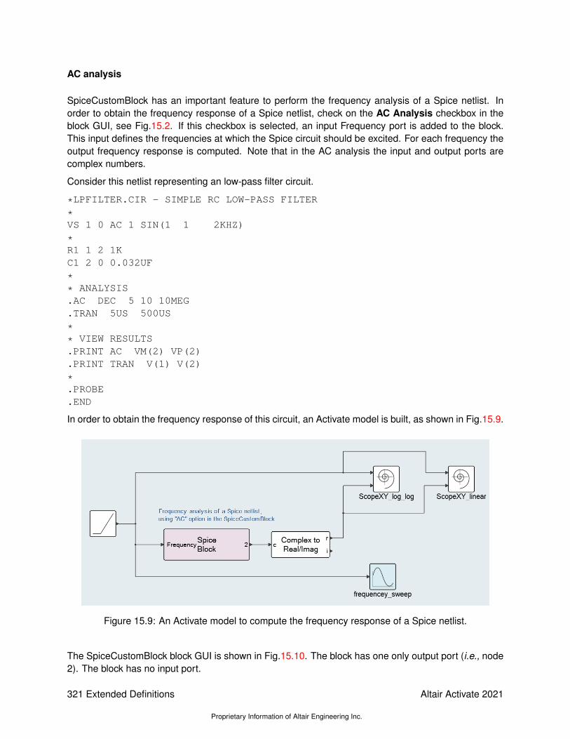
AC analysis
SpiceCustomBlock has an important feature to perform the frequency analysis of a Spice netlist. Inorder to obtain the frequency response of a Spice netlist, check on the AC Analysis checkbox in theblock GUI, see Fig.15.2. If this checkbox is selected, an input Frequency port is added to the block.This input defines the frequencies at which the Spice circuit should be excited. For each frequency theoutput frequency response is computed. Note that in the AC analysis the input and output ports arecomplex numbers.
Consider this netlist representing an low-pass filter circuit.
*LPFILTER.CIR - SIMPLE RC LOW-PASS FILTER
*VS 1 0 AC 1 SIN(1 1 2KHZ)
*R1 1 2 1KC1 2 0 0.032UF
** ANALYSIS.AC DEC 5 10 10MEG.TRAN 5US 500US
** VIEW RESULTS.PRINT AC VM(2) VP(2).PRINT TRAN V(1) V(2)
*.PROBE.END
In order to obtain the frequency response of this circuit, an Activate model is built, as shown in Fig.15.9.
Figure 15.9: An Activate model to compute the frequency response of a Spice netlist.
The SpiceCustomBlock block GUI is shown in Fig.15.10. The block has one only output port (i.e., node2). The block has no input port.
321 Extended Definitions
Proprietary Information of Altair Engineering Inc.
Altair Activate 2021

Figure 15.10: An Activate model to compute the frequency response of a Spice netlist.
A Ramp block has been used to sweep the frequency. The frequency is started from 1Hz and isincreased with a rate of 1KHz/Sec. The output of the ramp block is connected to the Frequency inputof the SpiceCustomBlock block. The filter output (i.e., node 2) is complex, so a Complex to Real/Imagblock is used to separate the complex and imaginary parts of the frequency response. The real partof output frequency response with respect to the input frequency is shown in Fig.15.11. Note thatfrequency axis is display on a logarithmic scale.
Figure 15.11: Frequency response of the low-pass filter for the model in Fig.15.9. Left plot is inLog-Log scale and the right plot is Linear-Log scale
Altair Activate 2021
Proprietary Information of Altair Engineering Inc.
Extended Definitions 322

Reporting
When a simulation of a Spice netlist fails, it is helpful to generate a logfile to find out the reason of thefailure. In order to create a logfile, click on the Reporting tab in the block GUI as shown in Fig.15.12.
Figure 15.12: GUI of the SpiceCustomBlock block for the report generator.
In the Spice interface logging level, the user can choose one of Nothing, Error, Warning,Info.
1. Nothing: No message is logged at all. This turns off the logger.
2. Error: Only error messages are logged.
3. Warning: Only Warning and error messages are logged.
4. Info: Every message emitted by the HyperSpice solver is logged.
The log filename should be specified. If a relative path is used, the file is created next to the model.
323 Extended Definitions
Proprietary Information of Altair Engineering Inc.
Altair Activate 2021

Altair Activate 2021
Proprietary Information of Altair Engineering Inc.
Extended Definitions 324

Chapter 16
Hybrid Automata in Altair Activate
16.1 Abstract
Hybrid automaton is a standard model for describing a hybrid system. A hybrid automaton is a statemachine augmented with differential equations and is generally represented by a graph composedof vertices and edges where vertices represent continuous activities and edges represent discretetransitions. Modeling a hybrid automaton with large number of vertices may be difficult, time-consumingand error prone using standard modules in modeling and simulation environments such as Activate. Inthis section, we present the Automaton block used for modeling and simulation of hybrid automata.
16.2 Introduction
Hybrid systems define a very wide class of dynamical systems that involve the interaction of hetero-geneous data types and dynamics especially the interaction of continuous-time dynamics describedby differential equations, with discrete dynamics described by a finite state under automata or othermodels of computation. Examples include mechanical systems with collisions, circuits with ideal diodesand switches, chemical processes controlled by valves or pumps, and most importantly, embeddedcomputation systems where digital devices interact with an analog environment.
Early works on formal models for hybrid systems includes phase transition systems and hybrid au-tomata. A hybrid automaton is a state machine augmented with differential equations. It is a standardmodel for describing a hybrid system. Hybrid automata come in several forms: The Alur-Henzingerhybrid automaton is a popular model that was developed primarily for algorithmic analysis of hybridsystems model checking [1, 2, 3]. In this document we will explain the way Activate environment canbe used to model and simulate hybrid systems, and in particular, hybrid automata.
Hybrid automata have been introduced by Xavier Nicollin et al. in [5] and an analysis of linear hybridautomata are given in [2, 4]. They modeled a hybrid system as a finite automaton that is expandedwith a set of real valued variables. These variables can be tested and modified at transitions. Atan automaton mode the value of variables change continuously with time according to evolution lawswhich are associated with the mode. The transition relations are specified by guarded commands; theactivities by differential equations; and the invariants by logical formulas. We now present the relevantdefinition of a hybrid automaton from Henzinger’s theory [4] that will be used in the construction of our
325 Extended Definitions
Proprietary Information of Altair Engineering Inc.
Altair Activate 2021

formal semantics for Activate automaton block.
H is a tuple which is defined as:H = (V,E,X, F, Invariant, Initial, Jump), where
• V is the set of control modes v1, . . . , vM where M is the number of control modes;
• E is the set of control switches which identify the source mode and a destination mode during atransition.
• X is a set of real-valued variables x1, . . . , xN where N is the dimension of H . X is first timederivative of X;
• F is a predicate over X, X assigned to each control mode; Invariant defines the admissiblerange for X, X in each mode;
• Initial defines initial values of X, X in each mode.
• Jump is an edge labeling function which assigns a predicate over X, X to each edge.
As an example consider the model of the bouncing ball in (16.1).x = vv = −g (16.1)
The model of this bouncing ball has been implemented in Activate as shown in Fig. 16.1.
Figure 16.1: The model of a control system in Activate
The output of the block JumpStateSpace is a vector of size two consisting of [x, v]t. Whenever thecondition (x < 0) is satisfied, an event is generated by the Zero-crossing (+ to - ) block. This eventmakes the Jump block do a reinitialization, i.e., v := −0.9v and x := x. In Fig. 16.1, the Clock blockgenerates periodic events (activation signals) to activate the Scope block which displays x and v.
This hybrid system can also be modeled as an automaton with a single control mode. The graphicalrepresentation of this automaton is depicted in Fig. 16.2. In this model, there are two variables x and vwhose initial values are given at t = 0. There are also two event sources; a zero-crossing event and aperiodic time event. Only the zero-crossing event causes discontinuity in variables.
Although it is often possible to model hybrid automata with generic Activate blocks, it is not an easyand efficient way to develop a hybrid automaton especially when the number of control modes is high.In a hybrid automaton composed of several control modes, at any time instant, only one mode or
Altair Activate 2021
Proprietary Information of Altair Engineering Inc.
Extended Definitions 326

Figure 16.2: Automaton for the bouncing ball
subsystem is active and the others should stay inactive. In Activate, even though it is possible togenerate an activation signal to activate conditionally a subsystem via If-Then-Else blocks, thevariables are still present in the state vector of the model and reduce the performance of the numericalsolver. Another difficulty is in detecting the jumps; in each control mode of the hybrid automaton,zero-crossing functions should be evaluated for monitoring the jump conditions. If we develop a hybridautomaton with several subsystems activated by If-Then-Else blocks, all zero-crossing functionsare active and it will be difficult to distinguish the zero-crossing functions that have to be monitored.Using switches and selector blocks, to activate or deactivate the zero-crossings, increases the modelsize and reduces the simulation speed.
Activate is a hybrid system simulator which means that Activate can simulate mixed continuous-timeand discrete-time subsystems. Developing hybrid automata containing large number of modes andcontinuous-time states [using generic Activate blocks] is a cumbersome, time-consuming, and difficulttask. In this section, we present the Automaton block used for modeling and simulation of hybridautomata. This block provides a modular way to model a general hybrid automaton in Activate. Thisblock provides an interface to model and encode the graphical representation of an automaton to beused by the simulator and consequently by the numerical solver in a completely transparent way.
16.3 Automaton Block
The automaton block provides a switching mechanism between subsystems corresponding to controlmodes of the automaton. Subsystems are constructed in such a way that they receive the state vectoras input from the automaton block and compute the flow and jump functions. The state variables aredefined only in the automaton block and not in the subsystems.
Suppose that a hybrid automaton consists ofM control modes. The continuous-time dynamics in mode’i’ is defined with DAE (0 = Fi(x, x, u)) where i ∈ 1 . . .M and the dimension of x is N (N ≥ 0) forany i ∈ 1 . . .M, as shown in Fig. 16.3. Suppose that in control mode ’i’, there are Zi jump conditionsindicating jumps toward other modes. The jump conditions are defined by Jumpij(x, x, u) functionswhere j ∈ 1 . . . Zi. When a jump function becomes positive a mode transition will happen. Whena transition to mode ’k’ happens state vector x is reset to Resetk(x, x, u), i.e., xl = Resetkl(x, x, u)for l ∈ 1 . . . N. Note that the reset function is identical for all incoming edges of mode k. In orderto develop an automaton containing a mode with multiple reset functions, the value of the current andprevious active modes should be used. These values are available at the first output port of the block.
327 Extended Definitions
Proprietary Information of Altair Engineering Inc.
Altair Activate 2021
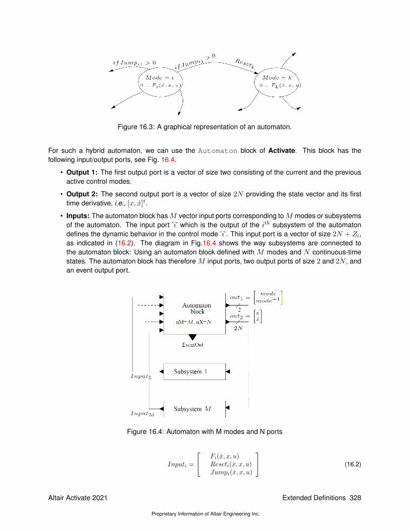
Figure 16.3: A graphical representation of an automaton.
For such a hybrid automaton, we can use the Automaton block of Activate. This block has thefollowing input/output ports, see Fig. 16.4.
• Output 1: The first output port is a vector of size two consisting of the current and the previousactive control modes.
• Output 2: The second output port is a vector of size 2N providing the state vector and its firsttime derivative, i.e., [x, x]t.
• Inputs: The automaton block hasM vector input ports corresponding toM modes or subsystemsof the automaton. The input port ’i’ which is the output of the ith subsystem of the automatondefines the dynamic behavior in the control mode ’i’. This input port is a vector of size 2N + Zi,as indicated in (16.2). The diagram in Fig.16.4 shows the way subsystems are connected tothe automaton block: Using an automaton block defined with M modes and N continuous-timestates. The automaton block has therefore M input ports, two output ports of size 2 and 2N , andan event output port.
Figure 16.4: Automaton with M modes and N ports
Inputi =
Fi(x, x, u)Reseti(x, x, u)Jumpi(x, x, u)
(16.2)
Altair Activate 2021
Proprietary Information of Altair Engineering Inc.
Extended Definitions 328

– The first N elements of the Inputi are the continuous-time dynamics. The dynamics of thesystem in the control mode ’i’ is described by a smooth index-1 DAE (i.e., 0 = Fi(x, x, u, t)).
– The next N elements of Inputi are the values used to reset the continuous-time stateswhen a transition to control mode ’i’ is activated.
– The next Zi elements of Inputi are the jump or zero-crossing functions. If the jth zero-crossing function of mode ’i’ crosses zero with negative to positive direction, a transition to’jth’ destination mode happens.
• Event Output: This is an event output port, which is activated whenever a mode transition hap-pens. This event is useful when an event is needed to activate or initialize a part of the subsystemnot included in the internal dynamics of the automaton block.
In order to parametrize the Automaton block, the user should double click on the block. Then the blockdialog opens and the user can enter the block parameters, as shown in Fig. 16.5.
Figure 16.5: Block dialog of the Automaton block
In the block dialog, the number of control modes, the initial control mode and the initial value ofcontinuous-time states at the beginning of the simulation should be given. Xproperties vector, coded inan M ×N matrix, indicates whether a continuous-time state is algebraic or differential in each controlmode. If a state is differential, its Xproperty should be set to "+1", otherwise it should be "-1". Xpropertycan be given as a 1×N vector if Xproperties of the states in all modes are identical.
The Jump fields express the mode transition information. Suppose that all control modes are labeledfrom 1 to M . Then, in the field corresponding to control mode ’i’, destination modes of mode ’i’ aredefined in a vector. jth element of this vector gives the destination mode when jth jump function(Jumpij(x, x, u)) becomes positive. For example, if in the field of the mode ’2’, the user defines [1; 3; 4],it means that in mode ’2’, there are three active jump functions. When, for example, the third jumpfunction becomes positive, a mode transition to mode ’4’ will be activated.
In order to illustrate the utility of this block for simplifying the development of hybrid automata models,the rest of this section is devoted to the implementation of two automata examples in Activate.
16.3.1 Example 1: Pendulum Swing Up
The inverted pendulum is a popular system for illustrating control problems. In [6], the hybrid controlstrategy for swinging up a pendulum from a downward to an upright position has been presented. Herewe will explain the way the pendulum and the control strategy can be modeled (and thus simulated) inActivate, using a hybrid automaton block.
329 Extended Definitions
Proprietary Information of Altair Engineering Inc.
Altair Activate 2021

Let x1 be the angle between the vertical axis and the pendulum, x2 the angular velocity, and u theapplied acceleration, which we consider as the control signal. Then, the dynamics of the system isgiven by
0 = f(x, x, u) =
−x1 + x2−x2 +ml(g sin(x1)− u cos(x1))/J
(16.3)
where g,m, l, J are the acceleration of gravity, the mass, the length, and the moment of inertia of thependulum. It can easily be shown that the input control force u defined with (16.4)
u =sin(x1) + x1 + x2
cos(x1)g (16.4)
brings the pendulum to the upward position with a single swing. Since the force of the pivot (u) islimited to [−um, um], the control force defined with (16.4) cannot be used. As a result, in order to bringthe pendulum up, more than one swing may be needed.
A swing-up control strategy suggested by Astrom and Furuta is based on a bang-bang control strategycontrolling the energy of the pendulum [6]. Assuming zero potential energy in the upward position, thetotal energy of the pendulum E is given by:
E = Jx222
+mgl(cos(x1)− 1) (16.5)
Starting from a negative energy in down position, the control strategy should bring up the pendulum tozero energy. To change the energy as fast as possible, the magnitude of the control signal should beas large as possible. The pendulum energy will become zero, if
dE2
dt= −mluEx2 cos(x1) < 0 (16.6)
This condition is fulfilled with the control law (16.7), which drives ‖E‖ to zero.
u = umsign(β)
β(x1, x2) = Ex2 cos(x1)(16.7)
The control law (16.7) results in chattering. Chattering can be avoided by using a saturation functioninstead of the sign function, i.e., the control law (16.8).
u = umsat(kβ) =
−um kβ < −1kumβ −1 < kβ < 1um 1 < kβ
(16.8)
The parameter k determines the region where the strategy is linear. In practice, k is determined bythe noise levels on the measured signals. When the pendulum arrives near the upward position, i.e.,cos(x1) > c1, the nonlinear controller (16.4) is applied to take over the control of the pendulum. Thispendulum system can be modeled with four control modes as shown in Fig. 16.6. Since following eachjump the states are re-initialized to last value of states in the previous mode, the initialization equationsare not shown.
The block dialog use to parametrize the Automaton block for this automaton is given in Fig. 16.5.The Activate model of this system is given in Fig. 16.7. There are four subsystems handled by this
Altair Activate 2021
Proprietary Information of Altair Engineering Inc.
Extended Definitions 330

Figure 16.6: Hybrid control strategy to swing up and stabilize an inverted pendulum on a cart
automaton block. As an example, the superblock SB2 corresponding to the control mode-2 is given inFig. 16.8.
The simulation result for a pendulum with mgl/J = 1, um = g/4, and x(0) = [π, 0]t is shown inFig. 16.9. The evolution of control modes and the pendulum angle and angular velocity (x1 and x2) aregiven in the first and the second subplots, respectively.
Figure 16.9: Simulation result for the model of Fig. 16.7
16.3.2 Example 2: DC/DC Buck Converter
Another hybrid system that shows an interesting dynamical behavior is the DC/DC buck converterwhose schematic circuit diagram is shown in Fig. 16.10. A buck converter is a step-down DC to DCpower supply composed of two electronic switches (a transistor and a diode), an inductor, and a capac-itor [7].
331 Extended Definitions
Proprietary Information of Altair Engineering Inc.
Altair Activate 2021
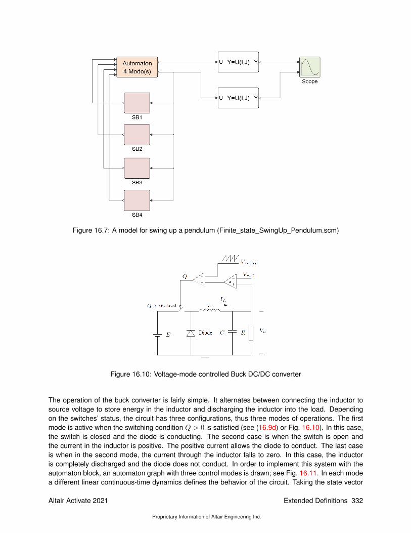
Figure 16.7: A model for swing up a pendulum (Finite_state_SwingUp_Pendulum.scm)
Figure 16.10: Voltage-mode controlled Buck DC/DC converter
The operation of the buck converter is fairly simple. It alternates between connecting the inductor tosource voltage to store energy in the inductor and discharging the inductor into the load. Dependingon the switches’ status, the circuit has three configurations, thus three modes of operations. The firstmode is active when the switching condition Q > 0 is satisfied (see (16.9d) or Fig. 16.10). In this case,the switch is closed and the diode is conducting. The second case is when the switch is open andthe current in the inductor is positive. The positive current allows the diode to conduct. The last caseis when in the second mode, the current through the inductor falls to zero. In this case, the inductoris completely discharged and the diode does not conduct. In order to implement this system with theautomaton block, an automaton graph with three control modes is drawn; see Fig. 16.11. In each modea different linear continuous-time dynamics defines the behavior of the circuit. Taking the state vector
Altair Activate 2021
Proprietary Information of Altair Engineering Inc.
Extended Definitions 332

Figure 16.8: Superblock SB2 in the model of Fig. 16.7
as x = [Vo, IL]t, we get (16.9a-16.9c). Note that the Xproperties of the states evolve: x2 is a differentialvariable in mode 1 and mode 2, and an algebraic variable in mode 3.
Figure 16.11: Hybrid automaton for a DC/DC Buck converter
0 = F1(x, x, u) =
RCx1 + x1 −Rx2Lx2 + x1 − E
(16.9a)
0 = F2(x, x) =
RCx1 + x1 −Rx2Lx2 + x1
(16.9b)
0 = F3(x, x) =
RCx1 + x1x2
(16.9c)
Q = Vramp − (x1 − Vref )a (16.9d)
The hybrid automaton of Fig. 16.11 has been implemented in Activate as given in Fig. 16.12.
333 Extended Definitions
Proprietary Information of Altair Engineering Inc.
Altair Activate 2021

Figure 16.12: Model (Finite_state_Buck.scm) for automaton given in Fig. 16.11
For the circuit, we have used the parameter values proposed in [8].
L = 20mH, C = 47µF, R = 110Ω,a = 8.4, VU = 8.2v, VL = 3.8v,Vref = 11.3v, E = 20v, T = 400µS
(16.10)
Depending on the value of R, the circuit operates in two or three operating modes. The simulationresult is given in Fig. 16.13. The first subplot is the evolution of the control mode during the simulation,the second subplot shows the output voltage, and the third subplot is the current through the inductor.It is interesting to note that the circuit exhibits a chaotic behavior as explained in [8, 9].
Altair Activate 2021
Proprietary Information of Altair Engineering Inc.
Extended Definitions 334

Figure 16.13: Simulation result for the model of Fig. 16.12
16.3.3 Example 3: Sticky balls
In this example ([10]), we consider two (sticky) masses on a flat frictionless table. As shown in Fig.16.14.Each of the balls is attached to a spring with distinct spring coefficient. If both balls are free, they willswing back and forth. However, if the two balls hit each other, they stick together. The stickiness isassumed to be exponentially decaying after they hit, and the decay speed is controlled by the parameter"Stickiness Decay" So after a while, they will separate.
Figure 16.14: Schematic of two sticky balls
The dynamical equation describing the movement of two masses are given in 16.11 and 16.12.
x1 = v1m1v1 = −k1(x1 − a1)
(16.11)
x2 = v2m2v2 = −k2(x2 − a2)
(16.12)
where x1, x2, v1, and v2 are position and velocity of masses. Whenever the condition (x1 >= x2)
335 Extended Definitions
Proprietary Information of Altair Engineering Inc.
Altair Activate 2021

becomes true two balls stick together. The dynamical equation of the stuck masses is given in 16.13.x3 = v3m3v3 = −k3(x3 − a3)
(16.13)
where x3 and v3 are position and velocity of the stuck balls andm3 = m1 +m2
k3 = k1 + k2a3 = k1∗a1+k2∗a2
a1+a2
(16.14)
The stickiness force is defined with the equation
s = −Cs
where C is the decay constant. At the sticking instant (te), x3, v3, and s are reinitialized to
x3(te) = x1v3(te) = m1v1+m2v2
m1+m2
s(te) = s0
(16.15)
where s0 is a constant. The stuck balls is subjected to two forces, the stickiness s and the separationforce which equal to
F = k1(x1 − a1)− k2(x2 − a2)
Once s < F becomes true, two balls separate. At the separation instant, states are reinitialized asfollows.
x1(te) = x2(te) = x3(te)v1(te) = v2(te) = v3(te)
(16.16)
The sticking balls can be modeled as a finite state system or an automation. There are two modes,separate and stuck as shown in Fig.16.15.
Figure 16.15: Hybrid automaton for sticky balls
In order to model this system in Activate with an automaton block, the automaton block should beparametrized as shown in Fig.16.16.
Altair Activate 2021
Proprietary Information of Altair Engineering Inc.
Extended Definitions 336

Figure 16.16: Parameterizing the Automaton block for the sticky masses model.
There are two modes and the continuous-time state size is four. Note that in this model number ofstates changes in each mode.
In the "separate" mode, the state vector X is composed of [x1, v1, x2, v2]. The residual vector deliveredto the first port of the Automaton block is 16.17.
0 =
−x1 + v1m1v1 + k1(x1 − a1)−x2 + v2m2v2 + k2(x2 − a2)
(16.17)
When a transition from "stuck" mode to "separate" model happens, the state vector X is reinitialized to[x3, v3, x3, v3]. The zero crossing function in the separate mode is:
g1 = x1 − x2 (16.18)
In the "stuck" mode, the state vector X is composed of [x3, v3, s, s]. The residual vector delivered tothe second port of the Automaton block is 16.19. The number of states of the block cannot change, asa result, in mode "stuck" we need a dummy state (q).
0 =
x3 = v3m3v3 = −k3(x3 − a3)s = −Csq = −q
(16.19)
When a transition from "separate" mode to "stuck" model happens, the state vector X is reinitialized to[x1,
m1v1+m2v2m1+m2
, s0, 1]. The zero crossing function in the separate mode is :
g2 = k1(x1 − a1)− k2(x2 − a2)− s (16.20)
The model is built in Activate using the an automaton block, the block diagram of the system is shownin Fig.16.17. The simulation result illustrating the position of masses (x1 and x2) is given in Fig.16.18.
337 Extended Definitions
Proprietary Information of Altair Engineering Inc.
Altair Activate 2021

Figure 16.17: Complete model of sticky masses (Automat_StickyMasses_decay.scm)
Figure 16.18: Position of masses.
Altair Activate 2021
Proprietary Information of Altair Engineering Inc.
Extended Definitions 338

16.4 conclusion
Hybrid automata are used to express hybrid dynamical systems. Although Activate is a general pur-pose hybrid system simulator, developing a hybrid automaton with several subsystems is difficult andtime-consuming. That is why the Automaton block is useful to allow straightforward construction ofhybrid automata. This block centralizes the control of the hybrid automaton and can simulate complexmulti-mode DAEs based on hybrid automata. This block can model different continuous-time dynamicsin each automaton mode.
339 Extended Definitions
Proprietary Information of Altair Engineering Inc.
Altair Activate 2021

Altair Activate 2021
Proprietary Information of Altair Engineering Inc.
Extended Definitions 340

Bibliography
[1] L. P. Carloni, R. Passerone, A. Pinto, and A. L. Angiovanni-Vincentelli, "Languages and tools forhybrid systems design,"Theoretical Computer Science, vol. 1, pp. 1-193, 2006.
[2] R. Alur, C. Courcoubetis, T. A. Henzinger, and P.-H. Ho, "Hybrid automata: An algorithmic approachto the specification and verification of hybrid systems," in Hybrid Systems, 1992, pp. 209-229. [On-line]. Available: citeseer.ist.psu.edu/alur92hybrid.html
[3] N. Lynch, R. Segala, F. Vaandrager, and H. Weinberg, "Languages and tools for hybrid systemsdesign in hybrid systems iii," Lecture Notes in Computer Science„ vol. 1066, pp. 496-510, 1996.
[4] T. A. Henzinger, "The theory of hybrid automata," Proceedings of the 11th Annual Symposium onLogic in Computer Science (LICS), pp. 278-292, 1996.
[5] X. Nicollin, J. Sifakis, and S. Yovine, "From ATP to timed graphs and hybrid sys-tems," Acta Informatica, vol. 30, no. 2, pp. 181-202, 1993. [Online]. Available: cite-seer.ist.psu.edu/article/nicollin93from.html
[6] K. J. Astrom and K. Furuta, "Swinging up a pendulum by energy control," Automatica, vol. 36, pp.278-285, 2000.
[7] M. di Bernardo, F. Garofalo, L. Glielmo, and F. Vasca, "Switching, bifurcations, and chaos in DC/DCconverters," IEEE Transactions on Circuits and Systems-I: Fundamental Theory and Applications,vol. 45, no. 2, pp. 133-141, Feb. 1998.
[8] E. Fossas and G. Olivar, "Study of chaos in the buck converter," IEEE Trans. on Circuits and Sys-tems I, vol. 43, pp. 13-25, 1996.
[9] F. E. guezar, ascal Acco, H. Bouzahir, and D. Fournier-Prunaret, "Chaotic behavior in a hybriddynamical system that arises from electronics," AIMS’ Sixth International Conference on Dyn. Sys-tems, Diff. Equations and Applications, Poitiers, France, 2006.
[10] http://sec.eecs.berkeley.edu/demo/StickyBall/StickyBall.htm
341 Extended Definitions
Proprietary Information of Altair Engineering Inc.
Altair Activate 2021

Altair Activate 2021
Proprietary Information of Altair Engineering Inc.
Extended Definitions 342

Chapter 17
Interpolation and extrapolation methodsin Activate
17.1 Introduction
Several blocks in Activate such as Lookup table, Signal generator, FromHDF, FromText,FromMat, FromCSV, and Signal-in generate continuous-time signals from discrete-time signals.The discrete-time signal variable provides the values of a signal Yi, at different time instants Xi. Thevalue of the signal at times other than elements of Xi are computed via interpolation or extrapola-tion. Several interpolation and extrapolation methods are available inside Activate blocks that will beexplained in the following sections. In order to illustrate each method, the method is applied on thisdata-set whose x-y diagram is shown in Fig.17.1.
X = [0, 1, 2, 4]Y = [4, 7, 6, 5]
Figure 17.1: x-y diagram for test data set.
343 Extended Definitions
Proprietary Information of Altair Engineering Inc.
Altair Activate 2021

17.2 Interpolation methods
The values of the signal at time instants inside the range [X1, XN ] are computed via interpolation.Several interpolation methods are available in Activate blocks:
• ZeroOrder, ZeroOrder(floor, Point_just_below): The index of element in X which is equal orbelow x is chosen to compute the output, i.e.,
for Xi ≤ x < Xi+1
y = Yi
The interpolation result is shown in Fig.17.2.
Figure 17.2: x-y diagram ZeroOrder, ZeroOrder(floor) methods.
• ZeroOrder(ceil, Point_just_above): The index of element in X which is equal or above x ischosen to compute the output, i.e.,
for Xi < x ≤ Xi+1
y = Yi+1
The interpolation result is shown in Fig.17.3.
Altair Activate 2021
Proprietary Information of Altair Engineering Inc.
Extended Definitions 344

Figure 17.3: x-y diagram ZeroOrder(ceil) methods.
• ZeroOrder(nearest, nearest_poin): The index of element in X which is nearest to x is chosento compute the output, i.e.,
forXi−1 +Xi
2≤ x < Xi +Xi+1
2
y = Yi
The interpolation result is shown in Fig.17.4.
Figure 17.4: x-y diagram ZeroOrder(nearest) methods.
• Linear. This is the default method and performs a linear interpolation. If x matches one of Xelements, the output is the corresponding element in the Y matrix. If no value matches, then
345 Extended Definitions
Proprietary Information of Altair Engineering Inc.
Altair Activate 2021

a linear interpolation is performed between two nearest elements of X to determine the outputvalue, i.e.,
for Xi ≤ x < Xi+1
y = Yi + (x−Xi)Yi+1 − YiXi+1 −Xi
The interpolation result is shown in Fig.17.5.
Figure 17.5: x-y diagram Linear methods.
• Bilinear interpolation: The bilinear interpolation is an extension of linear interpolation for inter-polating functions of two variables on a rectilinear 2D grid. In this method, first an interpolationin one direction is performed, and then again in the other direction. Although each step is linearin the sampled values and in the position, the interpolation as a whole is not linear but ratherquadratic in the sample location.
• Trilinear interpolation: The trilinear interpolation method is an interpolation on a 3-dimensionalregular grid which approximates the value of an intermediate point within the local axial rectan-gular prism linearly, using data on the lattice points. The trilinear interpolation is an extension oflinear interpolation for interpolating functions of three variables on a 3D grid. In this method, firstan interpolation in one direction is performed, and then again in the other directions. Althougheach step is linear in the sampled values and in the position, the interpolation as a whole is notlinear but rather cubic in the sample location.
• Not_a_knot: A cubic spline is computed by imposing following conditions (considering N pointsX1,...,XN ).
S(3)(X−2 ) = S(3)(X+
2 )
S(3)(X−N−1) = S(3)(X+N−1).
where S(n) is nth derivative of the interpolated curve.
Altair Activate 2021
Proprietary Information of Altair Engineering Inc.
Extended Definitions 346
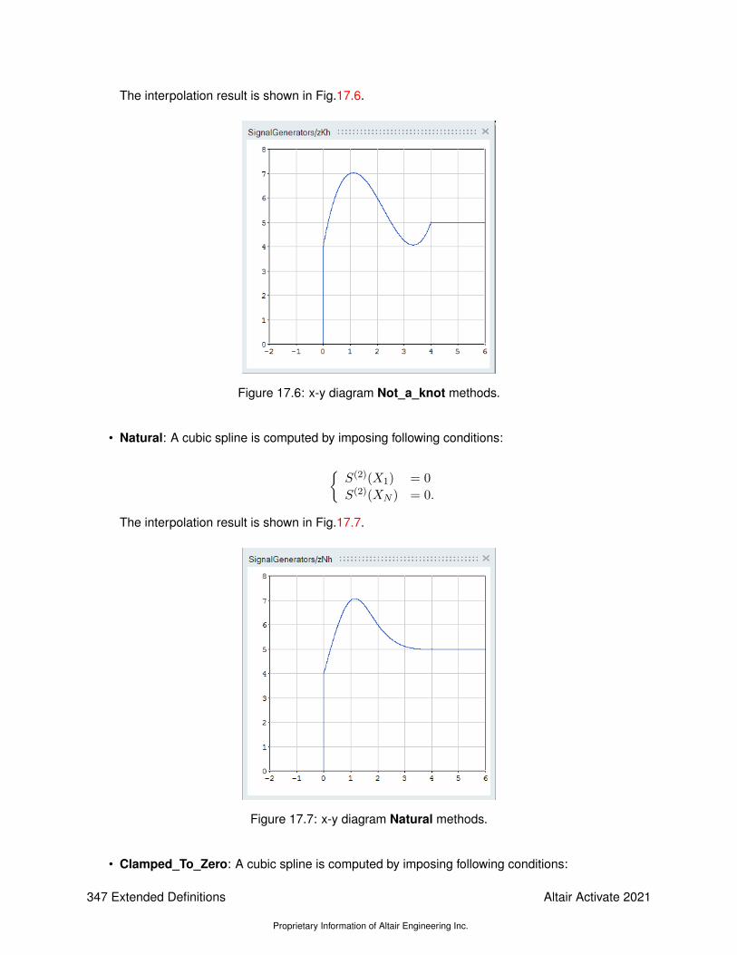
The interpolation result is shown in Fig.17.6.
Figure 17.6: x-y diagram Not_a_knot methods.
• Natural: A cubic spline is computed by imposing following conditions:
S(2)(X1) = 0
S(2)(XN ) = 0.
The interpolation result is shown in Fig.17.7.
Figure 17.7: x-y diagram Natural methods.
• Clamped_To_Zero: A cubic spline is computed by imposing following conditions:
347 Extended Definitions
Proprietary Information of Altair Engineering Inc.
Altair Activate 2021

S(1)(X1) = 0,
S(1)(XN ) = 0.
The interpolation result is shown in Fig.17.8.
Figure 17.8: x-y diagram Clamped_To_Zero methods.
• Akima interpolation method: The Akima interpolation method 1 is a continuously differentiablesub-spline interpolation method built from piecewise third order polynomials. This method pro-vides less ringing and overshoot than natural and not-a-knot spline algorithms. In this methodonly data from the next neighbor points is used to determine the coefficients of the interpolationpolynomial. Since no functional form for the whole curve is assumed and only a small number ofpoints is taken into account this method does not lead to unnatural values in the resulting curve.
• Fritsch-Butland interpolation method:
The Fritsch-Butland interpolation method 2 is a continuously differentiable cubic interpolationmethod built from piecewise third order polynomials. In this method local first derivative approxi-mations is used and guaranties to generate locally monotone interpolation curves.
• Steffen interpolation method:
The Steffen interpolation method 3 guarantees the monotonicity of the interpolating function be-tween the given data points. The minima and maxima can only occur exactly at the data points,and there can never be spurious oscillations between data points. The resulting curve is piece-wise cubic on each interval with the slope at each grid point chosen to ensure monotonicity andprevent undesired oscillations. The interpolated function is piecewise cubic in each interval. Thefirst-order derivative is guaranteed to be continuous everywhere, but the second derivative maybe discontinuous.
1Hiroshi Akima, ’A New Method of Interpolation and Smooth Curve Fitting Based on Local Procedures,’ Journal of theACM, Vol. 17, No. 4, pp. 589-602, 1970
2 F. N. Fritsch and J. Butland. ’A method for constructing local monotone piecewise cubic interpolants’. SIAM J. Sci. Statist.Comput., 5 (1984), pp. 300-304
3M.Steffen, "A simple method for monotonic interpolation in one dimension", Astron. Astrophys. 239, 443-450 (1990).
Altair Activate 2021
Proprietary Information of Altair Engineering Inc.
Extended Definitions 348

17.3 Extrapolation methods
The values of the signal at time instants outside of the range [X1, XN ] are computed by extrapolation.Several extrapolation methods are available in Activate blocks. Extrapolation can be applied either atthe left-side, i.e., for x < X1 or at the right-side, i.e., for x > XN .
• Zero:This is the default method. In this case, the output is zero for time instants out of signal’srange, i.e.,
for x < X1, y = 0.0
for x > XN , y = 0.0
The left-side Zero extrapolation result is shown in Fig.17.9.
Figure 17.9: x-y diagram for left-side Zero extrapolation methods.
The left-side and right-side Zero extrapolation result is shown in Fig.17.10.
349 Extended Definitions
Proprietary Information of Altair Engineering Inc.
Altair Activate 2021

Figure 17.10: x-y diagram for left-side and right-side Zero extrapolation methods.
• Hold: The output is equal to the last element of the Y vector, i.e.,for x < X1, y = Y1
for x > XN , y = YN
The left-side and right-side Hold extrapolation result is shown in Fig.17.11.
Figure 17.11: x-y diagram for left-side and right-side Hold extrapolation methods.
• Extrapolation. A linear extrapolation is performed using two left-most or right-most elements ofthe signal, i.e.,
for x < X1, y = Y1 + (x−X1)Y2−Y1X2−X1
for x > XN , y = YN−1 + (x−XN−1)YN−YN−1
XN−XN−1,
Altair Activate 2021
Proprietary Information of Altair Engineering Inc.
Extended Definitions 350

The left-side Extrapolation extrapolation result is shown in Fig.17.12.
Figure 17.12: x-y diagram for left-side Extrapolation extrapolation methods.
The right-side Extrapolation extrapolation result is shown in Fig.17.13.
Figure 17.13: x-y diagram for right-side Extrapolation extrapolation methods.
• Repeat. The signal is repeated over the whole range of X. For x < X1 or x > XN
y = y(x− k(XN −X1))
where k is an integer number to satisfy the following condition.
X1 ≤ x− k(XN −X1) < XN
351 Extended Definitions
Proprietary Information of Altair Engineering Inc.
Altair Activate 2021

The left-side Repeat extrapolation result is shown in Fig.17.14.
Figure 17.14: x-y diagram for left-side Repeat extrapolation methods.
The right-side Repeat extrapolation result is shown in Fig.17.15.
Figure 17.15: x-y diagram for right-side Repeat extrapolation methods.
17.3.1 Application - Behavior in blocks
The interpolation and extrapolation methods described above are available inside Activate blocks andare used to compute the value of the signal for inputs that are either before or after the data span.
In the following tables, all options and behaviors are described. The options can be set in the Advancedtabs of the blocks
Altair Activate 2021
Proprietary Information of Altair Engineering Inc.
Extended Definitions 352

Case with External Activation - Zero OrderSelected Action Left time span Right time span
Zero Zero ZeroHold Hold Hold
Extrapolation Hold HoldRepeat Repeat Repeat
Case without External Activation - Zero OrderSelected Action Left time span Right time span
Zero Zero HoldHold Hold Hold
Extrapolation Extrapolation ExtrapolationRepeat Repeat Repeat
Case without External Activation - LinearSelected Action Left time span Right time span
Zero Zero ZeroHold Hold Hold
Extrapolation Extrapolation ExtrapolationRepeat Repeat Repeat
353 Extended Definitions
Proprietary Information of Altair Engineering Inc.
Altair Activate 2021

Altair Activate 2021
Proprietary Information of Altair Engineering Inc.
Extended Definitions 354

Chapter 18
SignalOut and SignalIn blocks in AltairActivate
18.1 Introduction
A signal is an object used to define time dependent function over a given time span. Signals areoften defined and used in Activate but they are also accessible in the environment (OML workspace).Signals store time functions, mainly Activate simulation results, and also can provide input to Activatemodels. Signals also can be used for comparison and validation of simulation results, in particular inthe QA process. Signals can also be used as reference inputs in Activate models.
Signals can either be created and queried in OML using table commands, or be created and accessedin the Activate environment using SignalIn and SignalOut blocks, respectively. A Signal is a table in theOML environment composed of the time (time) and data (ch) fields. Following commands are usedto create a signal with name mysg.
• mysg= : This command is used to create the empty signal mysg in OML.
• mysg.time : The time field is a 3*N matrix where N is the number of time samples stored in thesignals structure.
– time vector : The first row of mysg.time matrix is the vector of the sampling time instants.
– event coding : The second row of mysg.time matrix is the event-coding (synchronizationinformation) of the corresponding sample. This coding will be explained in 18.2.
– event kind : The third row of mysg.time matrix indicates the kind of the event that hastriggered the sampling. The event kind will be explained in 18.2
• mysg.ch= : mysg.ch is a sub-table used for storing the set of data. Once mysg.ch created,data can be stored in the several channels. Each channel is a table composed of type and datafields.
• mysg.chi.type : Indicates the data-type of the ith channel, i.e., double, complex, int32,int32, int16, int8, uint32, uint16, uint8.
• mysg.chi.data: Represents the data stored in the ith channel and can be a matrix of size [Nrow,Ncol*N]. In fact, the data matrices of samples of size [Nrow*Ncol] are concatenated.
355 Extended Definitions
Proprietary Information of Altair Engineering Inc.
Altair Activate 2021

Example: Here is an example of a signals structure with two data sets.
B=;B.time=[1 2 4];B.ch=;B.ch1=;B.ch1.type=’double’;B.ch1.data=[1 2 3];B.ch2=;B.ch2.type=’int32’;B.ch2.data=[1 2 3 4 5 6;7 8 9 10 11 12];
Now you can use the "B" signal in a SignalIn block as we will see in following sections.
18.2 Activation information inside a signal object
Signal objects in Activate, contain specific information about how the SignalOut block has been acti-vated. An activation signal specifies the time instants where the signal may potentially change value.For example a discrete-time signal, which in Activate is simply a piece-wise constant function, has anactivation signal present at the points of potential discontinuities.
In general, an activation signal is a series of isolated points, called events, and intervals over time. Ifthe activation signal contains only isolated points, then we say that the corresponding signal is discrete-time. A special case of a discrete-time signal is the periodic signal where the activation points areequally spaced. But the latter property does not imply that a discrete-time signal is periodic, a periodicsignal must be declared as such. Activation intervals correspond to periods over which the signalevolves as a continuous-time function. The always-active signal is a special case of activation signalin which there exists a single activation interval covering the entire time period. A Activate signal ingeneral is made of multiple activation intervals. Over each such period, the corresponding time functionis supposed to be at least continuous and differentiable. Any point of discontinuity, in the value orthe derivative of the function, corresponds to a specific event. Two events may have the same time,therefore a Activate signal may take on successive values at the same time instant. The time event thatis not being used as an indexing mechanism can mean that based on the time values of the two eventsassociated with two different signals, nothing can be concluded as to their synchronization. Differentmethods can be used for coding signals over continuous-time activation periods. The method used heresamples the function and stores a list of time-value pairs, just as with event activations. An indicatorhowever distinguishes between the two types of "events".
Signals are typically created in Activate by the SignalOut blocks and read by the SignalIn blocks. Acti-vate signals are always considered asynchronous because each has its own activation signal.In order to preserve synchronization information between several data series, multiple data can beplaced together into one signal. In other words, a signal may contain several data series and a singletime vector. A Signal contains a time vector. For each time, the following information is associated:
Event-coding or synchronization information (accessed by GetNevIn(block) API) indicates theport[s] that has[ve ] been activated at the sampling time instants. remember binary coding of num-bers, for example, if an event activates the SignalOut via the input port 1, its coding 1. If an eventactivates the SignalOut via the input port 2, its coding is 2. if an event activates the SignalOut via theinput port 2 and 1, its coding is 3.
Altair Activate 2021
Proprietary Information of Altair Engineering Inc.
Extended Definitions 356
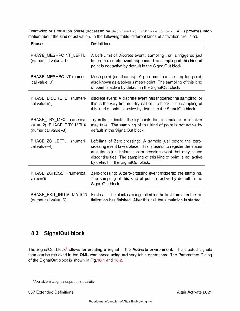
Event-kind or simulation phase (accessed by GetSimulationPhase(block) API) provides infor-mation about the kind of activation. In the following table, different kinds of activation are listed.
Phase Definition
PHASE_MESHPOINT_LEFTL(numerical value=-1)
A Left-Limit of Discrete event: sampling that is triggered justbefore a discrete event happens. The sampling of this kind ofpoint is not active by default in the SignalOut block.
PHASE_MESHPOINT (numer-ical value=0)
Mesh-point (continuous): A pure continuous sampling point,also known as a solver’s mesh-point. The sampling of this kindof point is active by default in the SignalOut block.
PHASE_DISCRETE (numeri-cal value=1)
discrete event: A discrete event has triggered the sampling, orthis is the very first non-try call of the block. The sampling ofthis kind of point is active by default in the SignalOut block.
PHASE_TRY_MFX (numericalvalue=2), PHASE_TRY_MRLX(numerical value=3)
Try calls: Indicates the try points that a simulator or a solvermay take. The sampling of this kind of point is not active bydefault in the SignalOut block.
PHASE_ZC_LEFTL (numeri-cal value=4)
Left-limit of Zero-crossing: A sample just before the zero-crossing event takes place. This is useful to register the statesor outputs just before a zero-crossing event that may causediscontinuities. The sampling of this kind of point is not activeby default in the SignalOut block.
PHASE_ZCROSS (numericalvalue=5)
Zero-crossing: A zero-crossing event triggered the sampling.The sampling of this kind of point is active by default in theSignalOut block.
PHASE_EXIT_INITIALIZATION(numerical value=6)
First-call: The block is being called for the first time after the ini-tialization has finished. After this call the simulation is started.
18.3 SignalOut block
The SignalOut block1 allows for creating a Signal in the Activate environment. The created signalsthen can be retrieved in the OML workspace using ordinary table operations. The Parameters Dialogof the SignalOut block is shown in Fig.18.1 and 18.2.
1Available in SignalExporters palette
357 Extended Definitions
Proprietary Information of Altair Engineering Inc.
Altair Activate 2021

Figure 18.1: Parameters Dialog of the SignalOut block.
Figure 18.2: Parameters Dialog of the SignalOut block (advanced tab).
The block has several parameters:
• Number of inputs: Used for specifying the number of data sets to be stored. This represents thenumber of elements in the ch field that will be available in the generated Signals. The data-typeof each channel can be different and is inherited from the source block.
• Variable name: Indicates the name of the signal generated in the OML environment.
• External activation: Once checked, the block samples its inputs only when the block is activatedby the incoming events.
• Buffer-size: The buffer indicates the number of samples to be stored. If number of samplesexceeds the size of the buffer, the earliest sample is replaced by the new one. If the user needsto keep all samples, the buffer-size should set to inf which means unlimited.
• Sampling filter: In many occasions, the user needs to register only specified kind of samples,e.g., only continuous-time samples or only discrete ones. These check boxes allow the userfiltering out unnecessary samplings points. Note that the event kind try would not generatesamples with increasing time samples. Note that in order to regenerate the signal by the SignalInblock, the time vector of the signal needs to be increasing.
Altair Activate 2021
Proprietary Information of Altair Engineering Inc.
Extended Definitions 358

18.4 SignalIn block
The SignalIn block2 reproduces the data series stored in the importing signal in the Activate environ-ment. The GUI of the SignalOut block is shown in Fig.18.3 and 18.4.
Figure 18.3: GUI of the signalIn block.
Figure 18.4: GUI of the signalIn block (advanced tab).
The block has several parameters:
• Variable name: The name of the signal to be retrieved from OML environment.
• Variable default value: If the requested signal name is not present in the OML environment, thisfiled allows providing a default value for the signal.
• Number of outputs: The SignalIn block needs the number of ch channels in the signal variable.Furthermore, for each channel, the data-size and data-type should be known, before reading thesignal variable. Otherwise an error signal will be emitted indicating the difference between theread signal and the given parameter in the GUI.
• Activated by the external events (ignore time): Once checked, all time information in the signal
2Available in SignalImporters palette
359 Extended Definitions
Proprietary Information of Altair Engineering Inc.
Altair Activate 2021

variable is ignored and external events trigger the output of the block. At each event trigger, anew sample is read.
• Generate event at discontinuities: This option allows generation events at sample times storedin the signal variable.
• Method: Indicates the interpolation method used for regeneration of the signal data series in theActivate environment. The acceptable values are:
– Zero-order (order 0)
– Linear (order 1)
– Not-a-knot (order 3)
– Natural (order 3)
– Clamped to zero (order 3)
These methods have been explained in the Interpolation methods chapter(17). When one of thedata types stored in the signal variable is not of type double, the interpolation method should bezero-order.
• Behavior before the start of the time data span: If the output value of a channel in a signalvalue is requested for a time instant before the start of the time span of the signal, this extrapola-tion method is used. The accepted values are:
– Zero: Output is zero.
– Extrapolation (Linear): The output is computed based on a linear extrapolation between firstand second data samples (if they exist).
– Hold: The output will be the value of the first data sample.
– Repeat: The output is computed to produce a periodic signal, repeating the whole time spanof the signal variable.
These methods has been explained in the Interpolation methods chapter(17).
• Behavior after the start of the time data span: If the output value of a channel in a signalvalue is requested for a time instant after the start of the time span of the signal, this extrapolationmethod is used. The accepted values are
– Zero: Output is zero.
– Extrapolation (Linear): The output is computed based on a linear extrapolation between twoend data samples (if they exist).
– Hold: The output will be the value of the final data sample.
– Repeat: The output is computed to produce a periodic signal, repeating the whole time spanof the signal variable.
These methods have been explained in the Interpolation Methods chapter (17).
Altair Activate 2021
Proprietary Information of Altair Engineering Inc.
Extended Definitions 360

Chapter 19
Animation
Currently Activate does not provide means to create sophisticated animations. The only block creatinganimations is the Anim2D block, which can be used to animate simple 2D graphical objects.
The block is based on OML functions to create figures and graphical objects, and define and modifytheir parameters. These functions can also be used directly by the user in an OML based block (forexample the OmlCustomBlock) to create custom animations. In most cases however the Anim2Dblock is easier to use. Some behaviors, for example graphical objects changing color during simulation,are not supported by the block and custom animation must be used. The OML functions also giveaccess to more properties such as the edge colors and thickness of some of the objects. The list ofthese OML functions can be found in OML documentations.
19.1 Anim2D block
The Anim2D block provided in the SignalViewers palette can be used to create 2D animations.Such animations are useful in particular to illustrate the behavior of simple mechanical and hydraulicssystems.
The Anim2D block can be used to animate different types of graphical objects in a Figure (on a canvas).The block has two input activation ports and a variable number of regular input ports.
Block regular inputs can be associated with different object types:
1. Type 1 is a closed polyline and the input signal is an N × 2 matrix where each row represents thex, y coordinates of a point of the polyline.
2. Type 2 is similar to type 1 but the polyline is not closed.
3. Type 3 corresponds to circles and the input is an M × 3 matrix. Each row corresponds to a circleand contains the x, y coordinates of the center of the circle and its radius.
4. Type 4 corresponds to rectangles and the input is a K × 4 matrix. Each row corresponds to arectangle and contains the x, y coordinates of the lower left corner of the rectangle, and its widthand height.
The block parameters are:
• Number of input ports (nin), i.e., the number of input signals.
361 Extended Definitions
Proprietary Information of Altair Engineering Inc.
Altair Activate 2021

• Object types: vector of size nin. If all types are identical, a scalar may be used.
• Canvas geometry: vector of size 4.
• Color table: a matrix with three columns representing the RGB values of each color (valuedbetween 0 and 1). A row including −1’s is considered transparent. The number of rows need notmatch the number of objects being animated. If the table is too small, colors are reused from thetop of the table.
• Zoom factor setting: correspondence between Figure coordinate values and the number of pointson screen.
When the block is activated through its first input activation port, the animation advances by movingall the objects to the positions specified by the current input signals. When it is activated through itssecond activation port, the objects are duplicated and a copy is frozen in place on the Figure in orderto create snapshots visible at the end of the simulation (useful for example for exporting the Figure asan image).
Object types can be given negative values (-1 instead of 1, -2 instead of 2, etc.) if they should beexcluded from snapshots. This is particularly useful for non-moving objects (such as background dec-orations) that need not be included in the snapshots multiple times.
19.2 Examples
19.2.1 Bouncing balls
The Activate bouncing balls demo contains the animation of an arbitrary number of balls bouncing (in2D) against each other and against the walls, floor and ceiling. The information available for animation isthe positions and the radii of the balls, and the positions of the walls, floor and ceiling. The coordinatesx and y of the center of balls are given by signals, the rest are constant parameters.
The top diagram of the bouncing balls demo is shown in Fig. 19.1. The content of the Animation SuperBlock is illustrated in Fig. 19.2. The Anim2D block is used with two inputs. The first is of type rectangleused to display the walls, floor and ceiling. The second input is of type circle and animate the balls. SeeFig. 19.3. The Anim2D block parameters are shown in Fig. 19.4.
Figure 19.1: The Bouncing balls block output vectors provide the x and y coordinates of the balls.
Altair Activate 2021
Proprietary Information of Altair Engineering Inc.
Extended Definitions 362

Figure 19.2: The content of the Animation Super Block.
Figure 19.3: The animation Figure.
Figure 19.4: The parameters of the Anim2D block. The rectangle is not filled (its content istransparent) and the ball colors are chosen randomly.
363 Extended Definitions
Proprietary Information of Altair Engineering Inc.
Altair Activate 2021

19.2.2 Control of tank water levels
The model considered here, lvel.scm, is made up of two connected water containers. The firstcontainer is supplied with water by a constant flow pump which can be turned on and off. This containeris connected via a pipe to a second container. The second container also has an exit pipe, which canbe opened and closed by a valve. It is opened at random times and closed after a constant delay.
A simple controller is used to keep the level of water in the second container close to a given valuewhile avoiding the water level in the fist container to go over a maximum value.
Denoting the water levels in the two tanks respectively h1 and h2, the flow f1 from container 1 to 2 canbe expressed as follows
f1 = α√
2g(h1 − h2)
and the flow out of the second container is
f2 =
β√
2gh2 if outflow valve is open0 otherwise
where the parameters α and β depend on the pipes geometry. The water levels in the containersdepend on the flows as follows
h1 = γ(fin − f1)h2 = δ(f1 − f2)
where fin is a constant f0 if the pump is on and 0 if it is off. The parameters γ and δ depend on containersurface areas.
The water levels are measured by two sensors. The sensor output yi depends on hi, i = 1, 2:
yi = τ(hi − yi), i = 1, 2.
The parameter τ corresponds to the time response of the sensors.
The control is of type hysteresis where the pump is turned on when y1 is below the maximum allowedand y2 below hdown. It is turned off if y1 goes above the maximum allowed or y2 above hup.
The full model is illustrated in Fig. 19.5.
Figure 19.5: The two water container level control model.
The container and flow diagrams are given in Figs. 19.6 and 19.7. The Animation block content isillustrated in Fig. 19.8.
Altair Activate 2021
Proprietary Information of Altair Engineering Inc.
Extended Definitions 364

Figure 19.6: The diagram used to model the containers.
Figure 19.7: The diagram used to model flows.
The Anim2D block is used here to draw polylines and rectangles to illustrate not only the water levels inthe containers but also the opening and closing of the exit valve and the state of the pump. A snapshotis given in Fig. 19.9.
19.2.3 Rolling disk on the ground
The demo wheelsim.scm contains an animation showing a wheel (disk) rolling on the ground. The3D animation is obtained by projecting the 3D geometry into 2D using a projection matrix. The modeltop diagram is shown in Fig. 19.10 and the modified Animation block in Fig. 19.11. This modification ismade to create snapshots of the wheel at regular times to obtain the picture shown in Fig. 19.12. Thesnapshot times correspond to events received by Anim2D block on its second input activation port.
One other change is required to make the snapshots visible: the type of the filled polyline representingthe floor must be set to −1. Otherwise the floor is drawn at every step snapshot overshadowing all theprevious snapshots of the wheel. This change is shown in Fig. 19.13.
365 Extended Definitions
Proprietary Information of Altair Engineering Inc.
Altair Activate 2021

Figure 19.8: The content of the Animation block.
Altair Activate 2021
Proprietary Information of Altair Engineering Inc.
Extended Definitions 366

Figure 19.9: A snapshot of the animation. In this case the left and right rectangles are white becausethe flow in (controlled by pump) and flow out (controlled by the exit valve), are zero.
367 Extended Definitions
Proprietary Information of Altair Engineering Inc.
Altair Activate 2021

Figure 19.10: The top diagram of the wheelsim demo.
Figure 19.11: The content of the Animation block.
Altair Activate 2021
Proprietary Information of Altair Engineering Inc.
Extended Definitions 368

Figure 19.12: The final image of the animation.
Figure 19.13: The modified dialog box of the Anim2D block.
369 Extended Definitions
Proprietary Information of Altair Engineering Inc.
Altair Activate 2021

Altair Activate 2021
Proprietary Information of Altair Engineering Inc.
Extended Definitions 370

Chapter 20
Blocks to execute OML and Pythonscripts interactively
The blocks ExecOMLScript and ExecPythonScript can be used in Activate models to run scripts,respectively in OML and in Python. The script associated with the block is ran by the user in the blockdiagram edtior interactively through the block GUI. Unlike other Activate blocks, these blocks do nothingduring simulation.
The main usage is to allow users to initialize the environment, for example by running a script to linearizea plant and construct a controller before running a simulation to validate the controller.
Unlike the Initialization script, which is executed at every simulation, the OML script in ExecOMLScriptis executed on demand. Such scripts can also be executed directly in OML prior to running simulations.The advantage of using a ExecOMLScript block is that the model is self contained (the script is includedin the model).
Two demo models are provided using the ExecOMLScript block, one for linearization and the other foroptimization. A demo is also provided to show the usage of the ExecPythonScript block.
20.1 ExecOMLScript blocks: examples
In most cases, the script associated with the ExecOMLScript block in the model must be executedbefore running a simulation. The execution of the script creates OML variables that are needed by thesimulator.
20.1.1 Controller design based on linearization
The inv_pendulum_lin_OML_exec.scmmodel contains the classical inverted pendulum on a cartsystem with a linear controller modeled by a state-space block. The controller (At,Bt, Ct,Dt) matricesare defined by the structure _syslin, if defined in the base environment. Otherwise they are definedso that the associated transfer function is zero (so no control). This is done in the top diagram Contextscript as follows:
_syslin=GetFromBase(’_syslin’,[]);
371 Extended Definitions
Proprietary Information of Altair Engineering Inc.
Altair Activate 2021

if isempty(_syslin)At=[];Bt=zeros(0,2);Ct=zeros(1,0);Dt=zeros(1,2);
elseAt=_syslin.a;Bt=_syslin.b;Ct=_syslin.c;Dt=_syslin.d;
end
The construction of the _syslin structure is done by linearizing the Super Block containing the modelof the cart-pendulum system and using the resulting linear system to construct an observer-based con-troller based on pole placement. This is done by the OML script associated with the ExecOMLScriptblock. By executing this script, the controller is computed, placed in the _syslin structure and savedin the base environment (the OML script runs in the base environment):
clear(’_syslin’);% vector of input port indices considered for linearizationinps = 1;% vector of output port indices considered for linearizationouts = [1,2];% Modified contextctx=struct; ctx.z0=0; ctx.th0=0; ctx.phi=0;
model=bdeGetCurrentModel;% Selected Super block to linearizesuperblock = ’pendulum’;
[A,B,C,D]=vssLinearizeSuperBlock(model,superblock,inps,outs,0,ctx);n=size(A,1);Kc=-place(A,B,-1*ones(1,n));Kf=-place(A’,C’,-2*ones(1,n)); Kf=Kf’;
At=A+B*Kc+Kf*C+Kf*D*Kc; Bt=-Kf; Ct=Kc;
_syslin.a=At; _syslin.b=Bt; _syslin.c=Ct; _syslin.d=[];
If the model is simulated without running the script, the cart pendulum system is simulated withoutcontrol and as expected the pendulum is not stabilized. On the other hand, if the script is run before,the pendulum is stabilized.
20.1.2 Controller design based on optimization
The car_min_time_opt_OML_exec.scm contains the model of a vehicle. The objective is to findthe best gear ratios so that the vehicle can travel 1 Km in least amount of time. The optimization isperformed over the gear rations gear and the gear changing times T.
Altair Activate 2021
Proprietary Information of Altair Engineering Inc.
Extended Definitions 372

This model has been used and explained earlier in the Optimization chapter. Here the script performingthe optimization is placed inside an ExecOMLScript block. The script finds the optimal values of gearand T. They are used during simulation is already computed, otherwise default values are used. Thisis done in the Initialization script of the model as follows:
T=GetFromBase(’T’,4*ones(4,1));gear=GetFromBase(’gear’,[3.2;1.8;1.3;1;.8]);
20.2 ExecPythonScript blocks: example
The demo model reinforcement_learning_python_exec.scm considers again the cart pen-dulum system but here the controller is designed using reinforcement learning.
The reinforcement learning process used for the controller design of this inverted pendulum on a cartsystem is based on the cart-pole system implemented by Rich Sutton et al. The code is inspired by the’gym’ environment CartPole and the corresponding example in stable-baselines package.1 ThePython code installs the required Python packages if needed.
The learning code is run by executing the Python script inside the ExecPythonScript block (this is donedouble-clicking on the block and ’Execute’-ing the Python script). The execution of the script takes afew minutes; at the end the result is saved in the model’s temporary folder. At this point the model canbe simulated. The controller obtained from the learning process is loaded by the PyCustomBlock andused during simulation to implement the feedback controller.
This implementation of the reinforcement learning requires that the model of the plant (cart-pendulumin this case) be expressed in Python. So the plant model is actually created twice (once in Activateinside the cart pendulum Super Block, and once in Python). So there is a risk of discrepancy betweenthe models.
An alternative to the above approach is to use the Activate model to create the code used by rein-forcement learning. This can be done by using the code generation capabilities of Activate to createa C code for the corresponding Super Block, and interface it in Python. In this approach not only theplant model is created only once (so simplicity and no risk of discrepancy) but the performance is alsoimproved since the reinforcement learning program runs simulations in C code instead of Python code.
The Activate model reinforcement_learning_python_Pcode.scm contains an implementa-tion of this approach. The OML script in the ExecOmlScript block must be executed first to generatethe C code for the cart pendulum Super Block. This code is compiled and linked with Python. Thenthe Python Script in the Reinforcement learning block must be executed. This runs the reinforcementlearning algorithm that creates the controller. Finally running the simulation of the model shows theresult of the application of the controller.
1https://pypi.org/project/stable-baselines/
373 Extended Definitions
Proprietary Information of Altair Engineering Inc.
Altair Activate 2021