g. cowan sussp65, st andrews, 16-29 august 2009 / statistical methods 2 page 1 statistical methods...
TRANSCRIPT

G. Cowan SUSSP65, St Andrews, 16-29 August 2009 / Statistical Methods 2 page 1
Statistical Methods in Particle PhysicsLecture 2: Limits and Discovery
SUSSP65
St Andrews
16–29 August 2009
Glen CowanPhysics DepartmentRoyal Holloway, University of [email protected]/~cowan

G. Cowan SUSSP65, St Andrews, 16-29 August 2009 / Statistical Methods 2 page 2
OutlineLecture #1: An introduction to Bayesian statistical methods
Role of probability in data analysis (Frequentist, Bayesian)
A simple fitting problem : Frequentist vs. Bayesian solution
Bayesian computation, Markov Chain Monte Carlo
Lecture #2: Setting limits, making a discovery
Frequentist vs Bayesian approach,
treatment of systematic uncertainties
Lecture #3: Multivariate methods for HEP
Event selection as a statistical test
Neyman-Pearson lemma and likelihood ratio test
Some multivariate classifiers:
NN, BDT, SVM, ...

G. Cowan SUSSP65, St Andrews, 16-29 August 2009 / Statistical Methods 2 page 3
Setting limits: Poisson data with backgroundCount n events, e.g., in fixed time or integrated luminosity.
s = expected number of signal events
b = expected number of background events
n ~ Poisson(s+b):
Suppose the number of events found is roughly equal to theexpected number of background events, e.g., b = 4.6 and we observe nobs = 5 events.
The evidence for the presence of signal events is notstatistically significant,
→ set upper limit on the parameter s, taking into consideration any uncertainty in b.

4
Setting limitsFrequentist intervals (limits) for a parameter s can be found by defining a test of the hypothesized value s (do this for all s):
Specify values of the data n that are ‘disfavoured’ by s (critical region) such that P(n in critical region) ≤ for a prespecified , e.g., 0.05 or 0.1.
If n is observed in the critical region, reject the value s.
Now invert the test to define a confidence interval as:
set of s values that would not be rejected in a test ofsize (confidence level is 1 ).
The interval will cover the true value of s with probability ≥ 1 .
G. Cowan SUSSP65, St Andrews, 16-29 August 2009 / Statistical Methods 2

G. Cowan SUSSP65, St Andrews, 16-29 August 2009 / Statistical Methods 2 page 5
Frequentist upper limit for Poisson parameterFirst suppose that the expected background b is known.
Find the hypothetical value of s such that there is a given smallprobability, say, = 0.05, to find as few events as we did or less:
Solve numerically for s = sup, this gives an upper limit on s at aconfidence level of 1.
Example: suppose b = 0 and we find nobs = 0. For 1 = 0.95,
→
[0, sup] is an example of a confidence interval. It is designed toinclude the true value of s with probability at least for any s.

G. Cowan SUSSP65, St Andrews, 16-29 August 2009 / Statistical Methods 2 page 6
Calculating Poisson parameter limits
Analogous procedure for lower limit slo.
To solve for slo, sup, can exploit relation to 2 distribution:
Quantile of 2 distribution
For low fluctuation of n this can give negative result for sup; i.e. confidence interval is empty.

G. Cowan SUSSP65, St Andrews, 16-29 August 2009 / Statistical Methods 2 page 7
Limits near a physical boundarySuppose e.g. b = 2.5 and we observe n = 0.
If we choose CL = 0.9, we find from the formula for sup
Physicist: We already knew s ≥ 0 before we started; can’t use negative upper limit to report result of expensive experiment!
Statistician:The interval is designed to cover the true value only 90%of the time — this was clearly not one of those times.
Not uncommon dilemma when limit of parameter is close to a physical boundary, cf. m estimated using E2 p2 .

G. Cowan SUSSP65, St Andrews, 16-29 August 2009 / Statistical Methods 2 page 8
Expected limit for on s if s = 0
Physicist: I should have used CL = 0.95 — then sup = 0.496
Even better: for CL = 0.917923 we get sup = 10!
Reality check: with b = 2.5, typical Poisson fluctuation in n isat least √2.5 = 1.6. How can the limit be so low?
Look at the mean limit for the no-signal hypothesis (s = 0)(sensitivity).
Distribution of 95% CL limitswith b = 2.5, s = 0.Mean upper limit = 4.44

G. Cowan SUSSP65, St Andrews, 16-29 August 2009 / Statistical Methods 2 page 9
Likelihood ratio limits (Feldman-Cousins)Define likelihood ratio for hypothesized parameter value s:
Here is the ML estimator, note
Define a statistical test for a hypothetical value of s:
Rejection region defined by low values of likelihood ratio.
Reject s if p-value = P(l(s) ≤ lobs | s) is less than (e.g. = 0.05).
Confidence interval at CL = is the set of s values not rejected.
Resulting intervals can be one- or two-sided (depending on n).
(Re)discovered for HEP by Feldman and Cousins, Phys. Rev. D 57 (1998) 3873.
G. Cowan SUSSP65, St Andrews, 16-29 August 2009 / Statistical Methods 2 page 10
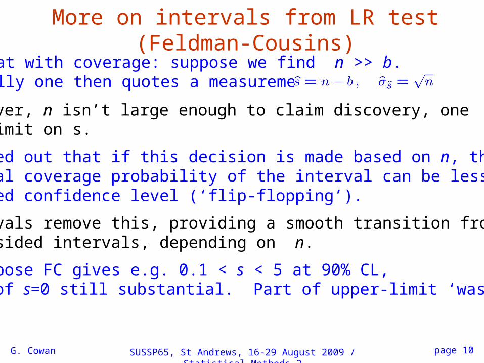
More on intervals from LR test (Feldman-Cousins)
Caveat with coverage: suppose we find n >> b.Usually one then quotes a measurement:
If, however, n isn’t large enough to claim discovery, onesets a limit on s.
FC pointed out that if this decision is made based on n, thenthe actual coverage probability of the interval can be less thanthe stated confidence level (‘flip-flopping’).
FC intervals remove this, providing a smooth transition from1- to 2-sided intervals, depending on n.
But, suppose FC gives e.g. 0.1 < s < 5 at 90% CL, p-value of s=0 still substantial. Part of upper-limit ‘wasted’?

11
Nuisance parameters and limitsIn general we don’t know the background b perfectly.
Suppose we have a measurement of b, e.g., bmeas ~ N (b, b)
So the data are really: n events and the value bmeas.
In principle the confidence interval recipe can be generalized to two measurements and two parameters.
Difficult and rarely attempted, but see e.g. talks by K. Cranmer at PHYSTAT03 and by G. Punzi at PHYSTAT05.
G. Punzi, PHYSTAT05
G. Cowan SUSSP65, St Andrews, 16-29 August 2009 / Statistical Methods 2

G. Cowan SUSSP65, St Andrews, 16-29 August 2009 / Statistical Methods 2 page 12
Nuisance parameters and profile likelihood
Suppose model has likelihood function
Parameters of interest Nuisance parameters
Define the profile likelihood ratio as
Maximizes L for given value of
Maximizes L
() reflects level of agreement between data and (0 ≤ () ≤ 1)
Equivalently use q = 2 ln ()

G. Cowan SUSSP65, St Andrews, 16-29 August 2009 / Statistical Methods 2 page 13
p-value from profile likelihood ratio Large q means worse agreement between data and
p-value = Prob(data with ≤ compatibility with when compared to the data we got | )
rapidly approaches chi-square pdf (Wilks’ theorem)
chi-square cumulativedistribution, degrees offreedom = dimension of
Reject if p < = 1 – CL
(Approx.) confidence interval for = set of values not rejected.
Coverage not exact for all but very good if
G. Cowan SUSSP65, St Andrews, 16-29 August 2009 / Statistical Methods 2 page 14
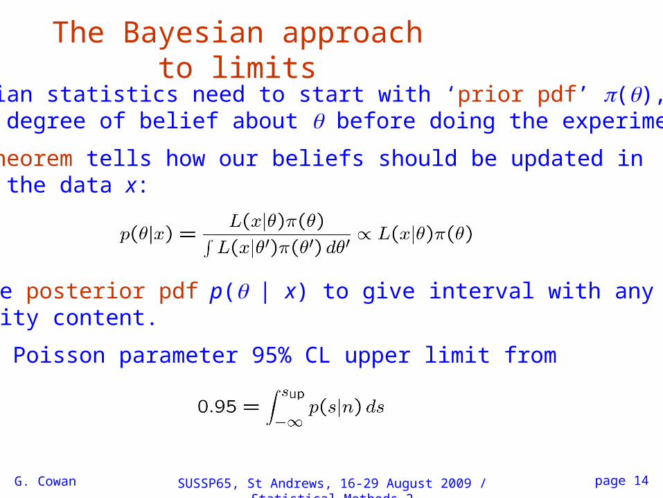
The Bayesian approach to limits
In Bayesian statistics need to start with ‘prior pdf’ (), this reflects degree of belief about before doing the experiment.
Bayes’ theorem tells how our beliefs should be updated inlight of the data x:
Integrate posterior pdf p(| x) to give interval with any desiredprobability content.
For e.g. Poisson parameter 95% CL upper limit from

G. Cowan SUSSP65, St Andrews, 16-29 August 2009 / Statistical Methods 2 page 15
Bayesian prior for Poisson parameterInclude knowledge that s ≥0 by setting prior (s) = 0 for s<0.
Often try to reflect ‘prior ignorance’ with e.g.
Not normalized but this is OK as long as L(s) dies off for large s.
Not invariant under change of parameter — if we had used insteada flat prior for, say, the mass of the Higgs boson, this would imply a non-flat prior for the expected number of Higgs events.
Doesn’t really reflect a reasonable degree of belief, but often usedas a point of reference;
or viewed as a recipe for producing an interval whose frequentistproperties can be studied (coverage will depend on true s).

G. Cowan SUSSP65, St Andrews, 16-29 August 2009 / Statistical Methods 2 page 16
Bayesian interval with flat prior for s
Solve numerically to find limit sup.
For special case b = 0, Bayesian upper limit with flat priornumerically same as classical case (‘coincidence’).
Otherwise Bayesian limit iseverywhere greater thanclassical (‘conservative’).
Never goes negative.
Doesn’t depend on b if n = 0.

G. Cowan SUSSP65, St Andrews, 16-29 August 2009 / Statistical Methods 2 page 17
Bayesian limits with uncertainty on bUncertainty on b goes into the prior, e.g.,
Put this into Bayes’ theorem,
Marginalize over b, then use p(s|n) to find intervals for swith any desired probability content.
Controversial part here is prior for signal s(s) (treatment of nuisance parameters is easy).

G. Cowan SUSSP65, St Andrews, 16-29 August 2009 / Statistical Methods 2 page 18
Frequentist discovery, p-values
To discover e.g. the Higgs, try to reject the background-only (null) hypothesis (H0).
Define a statistic t whose value reflects compatibility of datawith H0.
p-value = Prob(data with ≤ compatibility with H0 when compared to the data we got | H0 )
For example, if high values of t mean less compatibility,
If p-value comes out small, then this is evidence against the background-only hypothesis → discovery made!

G. Cowan SUSSP65, St Andrews, 16-29 August 2009 / Statistical Methods 2 page 19
Significance from p-value
Define significance Z as the number of standard deviationsthat a Gaussian variable would fluctuate in one directionto give the same p-value.
TMath::Prob
TMath::NormQuantile

G. Cowan SUSSP65, St Andrews, 16-29 August 2009 / Statistical Methods 2 page 20
When to publish
HEP folklore is to claim discovery when p = 2.9 10,corresponding to a significance Z = 5.
This is very subjective and really should depend on the prior probability of the phenomenon in question, e.g.,
phenomenon reasonable p-value for discoveryD0D0 mixing ~0.05Higgs ~ 107 (?)Life on Mars ~10
Astrology

G. Cowan SUSSP65, St Andrews, 16-29 August 2009 / Statistical Methods 2 page 21
Bayesian model selection (‘discovery’)
no Higgs
Higgs
The probability of hypothesis H0 relative to its complementaryalternative H1 is often given by the posterior odds:
Bayes factor B01 prior odds
The Bayes factor is regarded as measuring the weight of evidence of the data in support of H0 over H1.
Interchangeably use B10 = 1/B01

G. Cowan SUSSP65, St Andrews, 16-29 August 2009 / Statistical Methods 2 page 22
Assessing Bayes factors
One can use the Bayes factor much like a p-value (or Z value).
There is an “established” scale, analogous to our 5 rule:
B10 Evidence against H0
--------------------------------------------1 to 3 Not worth more than a bare mention3 to 20 Positive20 to 150 Strong> 150 Very strong
Kass and Raftery, Bayes Factors, J. Am Stat. Assoc 90 (1995) 773.
Will this be adopted in HEP?

G. Cowan SUSSP65, St Andrews, 16-29 August 2009 / Statistical Methods 2 page 23
Rewriting the Bayes factor
Suppose we have models Hi, i = 0, 1, ...,
each with a likelihood
and a prior pdf for its internal parameters
so that the full prior is
where is the overall prior probability for Hi.
The Bayes factor comparing Hi and Hj can be written

G. Cowan SUSSP65, St Andrews, 16-29 August 2009 / Statistical Methods 2 page 24
Bayes factors independent of P(Hi)
For Bij we need the posterior probabilities marginalized overall of the internal parameters of the models:
Use Bayestheorem
So therefore the Bayes factor is
The prior probabilities pi = P(Hi) cancel.
Ratio of marginal likelihoods

G. Cowan SUSSP65, St Andrews, 16-29 August 2009 / Statistical Methods 2 page 25
Numerical determination of Bayes factors
Both numerator and denominator of Bij are of the form
‘marginal likelihood’
Various ways to compute these, e.g., using sampling of the posterior pdf (which we can do with MCMC).
Harmonic Mean (and improvements)Importance samplingParallel tempering (~thermodynamic integration)Nested sampling...
See e.g.

G. Cowan SUSSP65, St Andrews, 16-29 August 2009 / Statistical Methods 2 page 26
Example of systematics in a searchCombination of Higgs boson search channels (ATLAS) Expected Performance of the ATLAS Experiment: Detector, Trigger and Physics, arXiv:0901.0512, CERN-OPEN-2008-20.
Standard Model Higgs channels considered (more to be used later): H → H → WW (*) → e H → ZZ(*) → 4l (l = e, ) H → → ll, lh
Used profile likelihood method for systematic uncertainties:background rates, signal & background shapes.

G. Cowan SUSSP65, St Andrews, 16-29 August 2009 / Statistical Methods 2 page 27
Statistical model for Higgs search
Bin i of a given channel has ni events, expectation value is
Expected signal and background are:
is global strength parameter, common to all channels. = 0 means background only, = 1 is SM hypothesis.
btot, s, b arenuisance parameters

G. Cowan SUSSP65, St Andrews, 16-29 August 2009 / Statistical Methods 2 page 28
The likelihood function
represents all nuisance parameters, e.g., background rate, shapes
here signal rate is only parameterof interest
The single-channel likelihood function uses Poisson modelfor events in signal and control histograms:
The full likelihood function is
There is a likelihood Li(,i) for each channel, i = 1, …, N.
data in signal histogramdata in control histogram

G. Cowan SUSSP65, St Andrews, 16-29 August 2009 / Statistical Methods 2 page 29
Profile likelihood ratioTo test hypothesized value of , construct profile likelihood ratio:
Maximized L for given
Maximized L
Equivalently use q =2 ln ():
data agree well with hypothesized → q small
data disagree with hypothesized → q large
Distribution of q under assumption of related to chi-square(Wilks' theorem, here approximation valid for roughly L > 2 fb-1):

G. Cowan SUSSP65, St Andrews, 16-29 August 2009 / Statistical Methods 2 page 30
p-value / significance of hypothesized
Test hypothesized by givingp-value, probability to see data with ≤ compatibility with compared to data observed:
Equivalently use significance,Z, defined as equivalent numberof sigmas for a Gaussian fluctuation in one direction:

G. Cowan SUSSP65, St Andrews, 16-29 August 2009 / Statistical Methods 2 page 31
SensitivityDiscovery:
Generate data under s+b ( = 1) hypothesis;Test hypothesis = 0 → p-value → Z.
Exclusion:Generate data under background-only ( =0) hypothesis;Test hypothesis .If has p-value < 0.05 exclude mH at 95% CL.
Presence of nuisance parameters leads to broadening of theprofile likelihood, reflecting the loss of information, and givesappropriately reduced discovery significance, weaker limits.

G. Cowan SUSSP65, St Andrews, 16-29 August 2009 / Statistical Methods 2 page 32
Combined discovery significance
Discovery signficance (in colour) vs. L, mH:
Approximations used here not always accurate for L < 2 fb1 but in most cases conservative.

G. Cowan SUSSP65, St Andrews, 16-29 August 2009 / Statistical Methods 2 page 33
Combined 95% CL exclusion limits
p-value of mH (in colour) vs. L, mH:
G. Cowan SUSSP65, St Andrews, 16-29 August 2009 / Statistical Methods 2 page 34
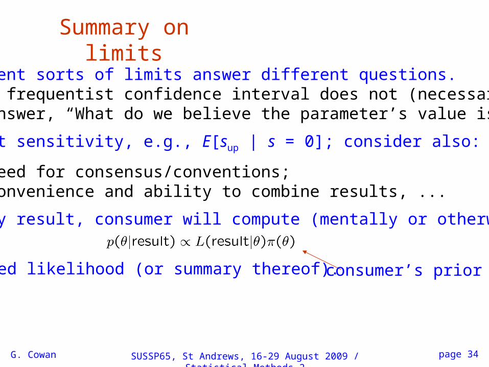
Summary on limits
Different sorts of limits answer different questions. A frequentist confidence interval does not (necessarily)answer, “What do we believe the parameter’s value is?”
Look at sensitivity, e.g., E[sup | s = 0]; consider also:
need for consensus/conventions;convenience and ability to combine results, ...
For any result, consumer will compute (mentally or otherwise):
Need likelihood (or summary thereof). consumer’s prior

G. Cowan SUSSP65, St Andrews, 16-29 August 2009 / Statistical Methods 2 page 35
Summary on discovery
Current convention: p-value of background-only < 2.9 × 10⁷ (5 )
This should really depend also on other factors:Plausibility of signalConfidence in modeling of background
Can also use Bayes factor
Should hopefully point to same conclusion as p-value.
If not, need to understand why!
As yet not widely used in HEP, numerical issues not easy.

G. Cowan SUSSP65, St Andrews, 16-29 August 2009 / Statistical Methods 2 page 36
Extra slides

G. Cowan SUSSP65, St Andrews, 16-29 August 2009 / Statistical Methods 2 page 37
Upper limit versus b
b
If n = 0 observed, should upper limit depend on b?Classical: yesBayesian: noFC: yes
Feldman & Cousins, PRD 57 (1998) 3873
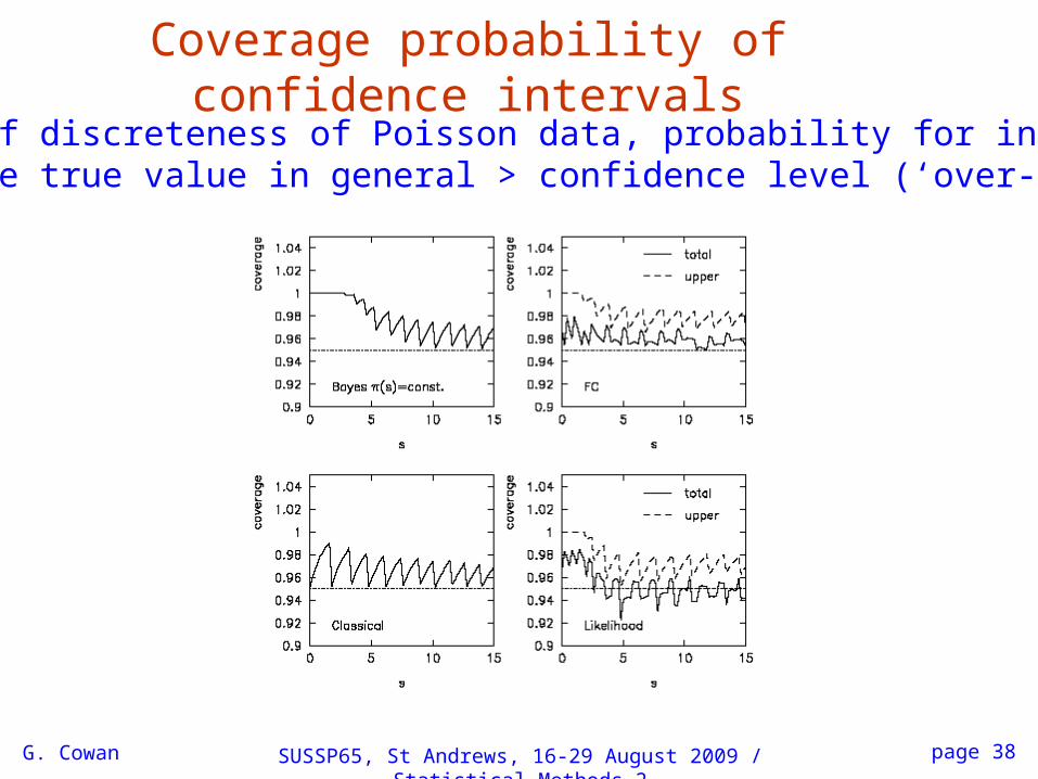
G. Cowan SUSSP65, St Andrews, 16-29 August 2009 / Statistical Methods 2 page 38
Coverage probability of confidence intervalsBecause of discreteness of Poisson data, probability for intervalto include true value in general > confidence level (‘over-coverage’)

39
Cousins-Highland method
Regard b as ‘random’, characterized by pdf (b).
Makes sense in Bayesian approach, but in frequentist model b is constant (although unknown).
A measurement bmeas is random but this is not the meannumber of background events, rather, b is.
Compute anyway
This would be the probability for n if Nature were to generatea new value of b upon repetition of the experiment with b(b).
Now e.g. use this P(n;s) in the classical recipe for upper limitat CL = 1 :
Result has hybrid Bayesian/frequentist character.
G. Cowan SUSSP65, St Andrews, 16-29 August 2009 / Statistical Methods 2

40Glen Cowan
‘Integrated likelihoods’
Consider again signal s and background b, suppose we haveuncertainty in b characterized by a prior pdf b(b).
Define integrated likelihood asalso called modified profile likelihood, in any case nota real likelihood.
Now use this to construct likelihood ratio test and invertto obtain confidence intervals.
Feldman-Cousins & Cousins-Highland (FHC2), see e.g.J. Conrad et al., Phys. Rev. D67 (2003) 012002 and Conrad/Tegenfeldt PHYSTAT05 talk.
Calculators available (Conrad, Tegenfeldt, Barlow).
RHUL HEP seminar, 22 March, 2006

G. Cowan SUSSP65, St Andrews, 16-29 August 2009 / Statistical Methods 2 page 41
Analytic formulae for limitsThere are a number of papers describing Bayesian limitsfor a variety of standard scenarios
Several conventional priorsSystematics on efficiency, backgroundCombination of channels
and (semi-)analytic formulae and software are provided.
But for more general cases we need to use numerical methods (e.g. L.D. uses importance sampling).

G. Cowan SUSSP65, St Andrews, 16-29 August 2009 / Statistical Methods 2 page 42
Harmonic mean estimator
E.g., consider only one model and write Bayes theorem as:
() is normalized to unity so integrate both sides,
Therefore sample from the posterior via MCMC and estimate m with one over the average of 1/L (the harmonic mean of L).
posteriorexpectation
G. Cowan SUSSP65, St Andrews, 16-29 August 2009 / Statistical Methods 2 page 43
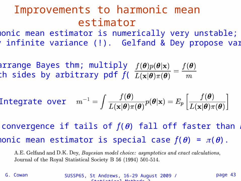
Improvements to harmonic mean estimator
The harmonic mean estimator is numerically very unstable;formally infinite variance (!). Gelfand & Dey propose variant:
Rearrange Bayes thm; multiply both sides by arbitrary pdf f():
Integrate over :
Improved convergence if tails of f() fall off faster than L(x|)()
Note harmonic mean estimator is special case f() = ()..

G. Cowan SUSSP65, St Andrews, 16-29 August 2009 / Statistical Methods 2 page 44
Importance sampling
Need pdf f() which we can evaluate at arbitrary and alsosample with MC.
The marginal likelihood can be written
Best convergence when f() approximates shape of L(x|)().
Use for f() e.g. multivariate Gaussian with mean and covarianceestimated from posterior (e.g. with MINUIT).