gabriel kron: num. sol'n of ode's & pde's by means...

Gabriel Kron: Num. Sol'n of ODE's & PDE's by Means of Equvalent ... http://www.quantum-chemistry-history.com/Kron_Dat/Kron-1945/Kr...

1 of 20 8/2/2005 11:09 PM

Journal of Applied Physics 16, 172-186 (1945)

{This website: Please note: The following article is complete; it has been put into ASCII due to a) space requirement reductionand b) for having thus the possibility to enlarge the fairly small figures. And: special math. symbols are in Unicode. Further: disallow M$-IE 'automatic picture size adaptation'.}

Abstract: Numerical methods are developed to solve certain types of linear and nonlinear partial differential equations to anydesired degree of accuracy with the aid of equivalent electrical networks. The methods of solution of ordinary differentialequations, both linear and nonlinear, follow as special cases. Three types of problems are considered:

1. Initial-value problems. If the field quantities are known along a surface, the networks may be solved by a straight-forwardstep-by-step calculation The networks may also be looked upon as supplying a 'schedule' of operations that can be put on adigital calculating machine.

For time-varying problems new types of networks are developed in which time appears as an extra spatial variable. Examples ofnew networks for the elastic field and for the general nonlinear wave equation are given. Sample calculations and theoreticalchecks of a transient heat flow problem and of an ordinary differential equation are also included.

2. Boundary-value problems. Four methods of solution are given, the first three being cut and try processes. (a) The method of weighted averages; (b) The method of unbalanced currents and voltages; (c) The 'relaxation' method;(d) The 'diffusion' method, that changes the boundary-value problem into an initial-value problem by adding to the originalpartial differential equation a time variable of the form A?f /?t, allowing the unbalanced currents to 'diffuse' in time.

These numerical methods may also be used to improve the accuracy of the results found on the Network Analyzer. Examples ofcalculations are given for the electromagnetic and the elastic fields.

3. Characteristic-value problems. Their methods of solution are similar to those of boundary-value problems. An additionalmethod of unbalanced admittances is also indicated. It is shown that by calculating the power in the network, the characteristicvalue of the assumed function is 'found'.

An improved characteristic value of the linear harmonic oscillator, solved initially on a Network Analyzer, is calculated as anexample.

In general the electrical networks may-be used to check the consistency and correctness of solutions arrived at by othermethods, approximate or exact. The unbalanced currents at the junctions (easily calculated) give a quantitative measure of thedeviation from the correct solution.

NETS

The method of solving partial differential equations numerically by the use of equivalent circuits is by no means new. It has long beenknown (1,2) that Laplace equation ? 2f = 0 in rectangular coordinates may be solved to any desired degree of accuracy by(considering the two-dimensional case) drawing a net of squares, Fig. 1, each with area ?x?y, and associating with each line the realpositive number, unity. If with each junction (representing a point of space) the correct value of the dependent variable f is associated,

then each f must be the average of the four neighboring f 's. An extension of this method to Poisson’s equation ? 2f = k, where k is anarbitrary function, has also been in use.

The equivalent circuits presented here may be looked upon as generalizations to more general partial differential equations of the type


2 of 20 8/2/2005 11:09 PM

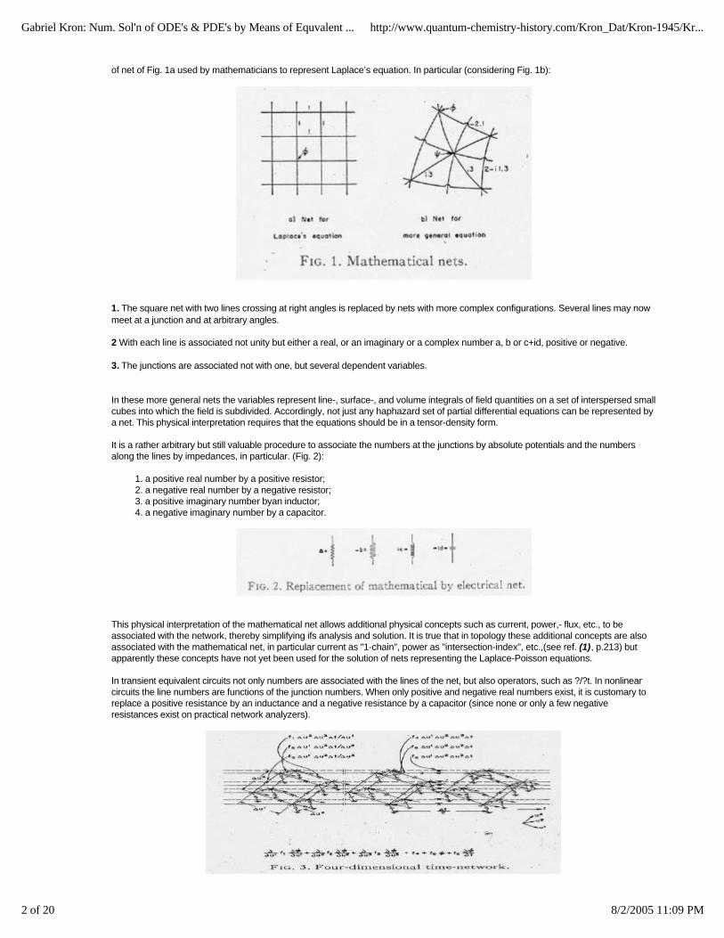
of net of Fig. 1a used by mathematicians to represent Laplace’s equation. In particular (considering Fig. 1b):

1. The square net with two lines crossing at right angles is replaced by nets with more complex configurations. Several lines may nowmeet at a junction and at arbitrary angles.

2 With each line is associated not unity but either a real, or an imaginary or a complex number a, b or c+id, positive or negative.

3. The junctions are associated not with one, but several dependent variables.

In these more general nets the variables represent line-, surface-, and volume integrals of field quantities on a set of interspersed smallcubes into which the field is subdivided. Accordingly, not just any haphazard set of partial differential equations can be represented bya net. This physical interpretation requires that the equations should be in a tensor-density form.

It is a rather arbitrary but still valuable procedure to associate the numbers at the junctions by absolute potentials and the numbersalong the lines by impedances, in particular. (Fig. 2):

1. a positive real number by a positive resistor;2. a negative real number by a negative resistor;3. a positive imaginary number byan inductor;4. a negative imaginary number by a capacitor.

This physical interpretation of the mathematical net allows additional physical concepts such as current, power,- flux, etc., to beassociated with the network, thereby simplifying ifs analysis and solution. It is true that in topology these additional concepts are alsoassociated with the mathematical net, in particular current as "1-chain", power as "intersection-index", etc.,(see ref. (1), p.213) butapparently these concepts have not yet been used for the solution of nets representing the Laplace-Poisson equations.

In transient equivalent circuits not only numbers are associated with the lines of the net, but also operators, such as ?/?t. In nonlinearcircuits the line numbers are functions of the junction numbers. When only positive and negative real numbers exist, it is customary toreplace a positive resistance by an inductance and a negative resistance by a capacitor (since none or only a few negativeresistances exist on practical network analyzers).


3 of 20 8/2/2005 11:09 PM

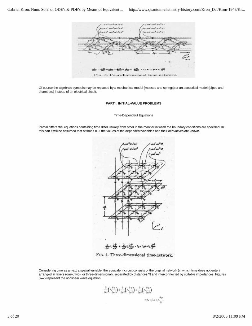
Of course the algebraic symbols may be replaced by a mechanical model (masses and springs) or an acoustical model (pipes andchambers) instead of an electrical circuit.

PART I. INITIAL-VALUE PROBLEMS

Time-Dependeut Equations

Partial differential equations containing time differ usually from other in the manner in whith the boundary conditions are specified. Inthis part it will be assumed that at time t = 0, the values of the dependent variables and their derivatives are known.

Considering time as an extra spatial variable, the equivalent circuit consists of the original network (in which time does not enter)arranged in layers (one-, two-, or three-dimensional), separated by distances ?t and interconnected by suitable impedances. Figures3—5 represent the nonlinear wave equation,


4 of 20 8/2/2005 11:09 PM

for various numbers of independent variables.

In orthogonal curvilinear coordinates

where the f ’s are arbitrary functions of u1, u2, u3, and t.


5 of 20 8/2/2005 11:09 PM

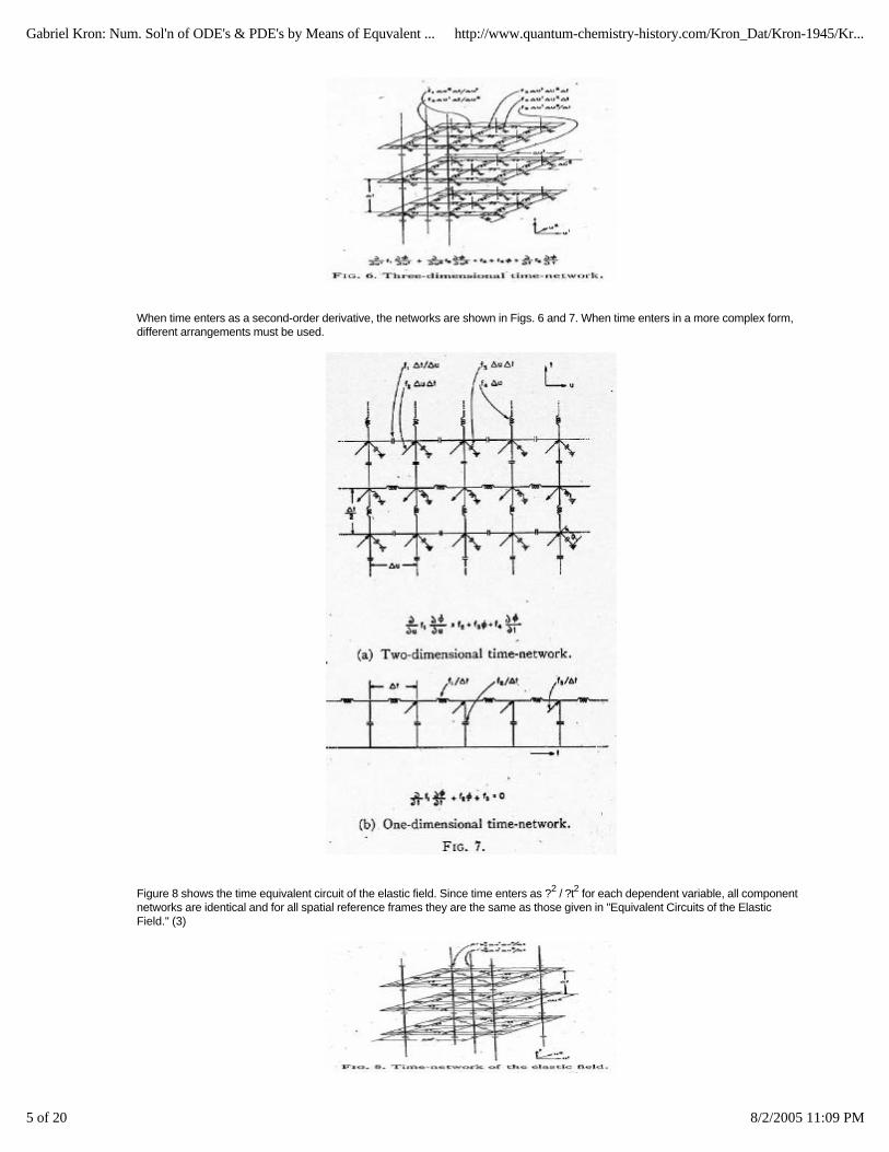
When time enters as a second-order derivative, the networks are shown in Figs. 6 and 7. When time enters in a more complex form,different arrangements must be used.

Figure 8 shows the time equivalent circuit of the elastic field. Since time enters as ?2 / ?t2 for each dependent variable, all componentnetworks are identical and for all spatial reference frames they are the same as those given in "Equivalent Circuits of the ElasticField." (3)


6 of 20 8/2/2005 11:09 PM

It should be noted that while in the elastic and fluid flow fields the time coordinate may be left out or included at will, such is not the casein the electromagnetic field. In the latter the non-privileged role of the time coordinate necessitates a radically new treatment.

Time as a Spatial Variable

Let in a linear problem at t = 0 an instantaneous impulse be impressed on the physical system. On the network this impulse isimpressed by generators at t = 0 and the voltage distribution gives the effect of the impulse in time and in space. (In the absence of aNetwork Analyzer the voltage distribution may be found by the methods to be shown presently.) Since the network extends to infinityalong time, the network beyond any specified time t0 may be replaced by a characteristic impedance.

If the effects of an impulse are known, then the effect of any other force applied within any time interval may be found by simplesuperposition of the known voltage distribution.

It should be noted that the effect of more than one impulse cannot be studied simultaneously on the Networkl Analyzer, since agenerator impressed, say, at t = 5?t produces a voltage distribution at points corresponding to previous times, a situation impossiblein classical dynamical problems. The numerical method to be shown prevents this "backsliding" of the impulses impressed at varioustimes.

The Numerical Calculations

The numerical method is based on the fact that if all the potentials on the network are defined at t = n?t and at t = (n+1)?t (and also theboundary conditions along time), then all the potentials and currents'càn be calculatçd for the rest of the hetwork in a straightforwardmanner up to any desired number of ?t's.

The numerical work consists of calculating all the admittances and currents on the second or (n+1)?t network, (Since in nonlinearproblems the admittances are functions of the potentials, the former can all be calculated.) Adding up at a junction all the currents,induding the one coming from the lower network, the resultant current must flow upward to the next network (n+2)?t, Fig. 4. Since theadmittance of the connecting coil is known (even in nonlinear

problems) the absolute potentials of the corresponding points on the next network (n+2)?t are thereby determined. The work ofcalculating currents is again repeated to proceed to the next network at (n+3)?t.

Starting Assumptions

It should be noted that in order to get started, it is necessary to know not only all the currents on the network say at t = 0 but also thecurrents coming from the next lower network, t = - ?t. However, in most problems the boundary conditions are so defined that at t = 0the currents coming from the lower network are not known, although the sum of the lower and upper connecting currents, namely ?t(?f /?t) is known at every point. At the start of each problem thus the question arises how to divide the resultant currents into two parts at t= 0. Several methods are available:

(1) Half the current may be assumed to flow up, the other down. This assumes the slope of the curve f = f(t) to be constant in theneighborhood of t = 0. After proceeding through two or three layers of networks it is possible to discern a more logical division thanhalving and to start all over again with the new divisions.

(2) Standard methods of approximations given in textbooks (4) may be used. For instance, after finding the potentials on the t = ?t


7 of 20 8/2/2005 11:09 PM

network, the differences of potentials between the two networks define the slope of the chord between the points t = 0 and t = ?t. Usingthis slope instead of that of the tangent ?t(?f / ?t) at t = 0, a better division is accomplished. This step may be repeated several timesbetween the first two networks.

(3) ?t maybe subdivided into 5 or more subdivisions. Because of the finer divisions the results arrived at by the 5th ?t may beassumed to be close enough approximations and may be used as starting values on the coarser network.

Other Assumptions

Since the starting conditions are rarely known exactly, it will often be found that the currents or voltages in successive steps do not lieon smooth curves but oscillate around them in an attempt to correct themselves. Such overshooting and undershooting of smoothcurves may be minimized by judicious changing at intervals of the division of currents that flow "up" and "down" between the layers.Most numerical methods do not possess this self-correcting property of the equivalent circuits.

When some of the admittances lying between two successive layers (between two ?t's) are functions of the dependent variables(hence, of time) their value has to be found by extrapolating from the known values of the dependent variables at two previous times.

Ordinary Differential Equations

In ordin~ary differential equations the independent variable may be either a spatial variable x or time t. If it happens to be the time, thenusually sufficient information is available at t = 0 to get the calculations started as above.

When the independent variable x is a spatial variable then usually only part of the boundary conditions (say the value of f ) are definedat x = 0. Some boundary conditions (say the slope, of f ) may, however, be defined only at x = a. In such cases it is possible to start outwith a tentative slope at x = 0 and find with the above step-by-step method the slope at x = a. Several new starts should eventuallymatch the boundary conditions at the two different values of x.

An example,

di/dt = 10 - 2i

with initial conditions i = 0 and t = 0 (also di/dt =10 at t=0) is worked out in Fig. 9 in steps of ?t= 0.1. The numerals in parenthesis givethe results found in Doherty and Keller (5) for the same problem, found by a standard method requiring a cut and try procedure not onlyat the first step (between t = 0 and t = ?t) but at every step.

Other worked out examples may be found in "The Application of Network Analysis to Some Electron Optical Problems." (13)

Example of a Transient Heat Flow Problem

Let the temperature at the edge of a plate be raised from zero to unit temperature at t = 0 and be kept at that same temperature. Theproblem is to find the distribution of temperature along the plate (at distance x from the edge) at various times.

The equation of flow is

Also ?x=0.1, a?t=0.0025. Hence ?t=0.0024/a


8 of 20 8/2/2005 11:09 PM

The boundary conditions are:

Since the known data at t = 0 are rather meager (T and ?T / ? t are zero at every point along x except near x = 0) for a preliminarycalculation the assumed ?t is subdivided into five parts, so that a?t = 0.0005. The corresponding network to be used to get started isshown in Fig. 10.

The layer at t = 0 only contains one current 5 flowing into the ground. (The existence of a ground is a boundary condition.) Hence thiscurrent cannot very well be assumed to divide into two equal parts. Instead, let it be assumed that a similar current in the next layer att=a?t/2 also has a value 5. Now half of that may flow up and half down. Assuming slightly less than half, say 2.45 flowing up, onepotential on the next layer is 24.5. Its neighboring potential on the same layer is still undetermined but it must be small and could aswell be assumed to be zero for the purpose of calcijilating the current flowing into this junction. The latter (24.5 - 0) 0.005 = 0.1225 isassumed again to flow half up, half down.

Continuing the calculation through five layers, the voltages on the fifth layer can be assumed to be approximately correct. Since the firstlayer contains too few informations, the calculation is continued to the tenth layer in order to be able to use the fifth and tenth layers asthe first two layers of the coarser network of Fig. 11.


9 of 20 8/2/2005 11:09 PM

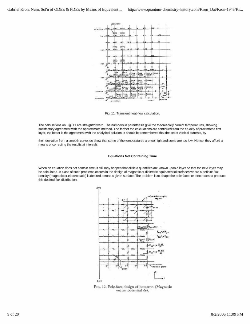
Fig. 11. Transient heat-flow calculation.

The calculations on Fig. 11 are straightforward. The numbers in parenthesis give the theoretically correct temperatures, showingsatisfactory agreement with the approximate method. The farther the calculations are continued from the crudely approximated firstlayer, the better is the agreement with the analytical solution. It should be remembered that the set of vertical currents, by

their deviation from a smooth curve, do show that some of the temperatures are too high and some are too low. Hence, they afford ameans of correcting the results at intervals.

Equations Not Containing Time

When an equation does not contain time, it still may happen that all field quantities are known upon a layer so that the next layer maybe calculated. A class of such problems occurs in the design of magnetic or dielectric equipotential surfaces where a definite fluxdensity (magnetic or electrostatic) is desired across a given surface. The problem is to shape the pole faces or electrodes to producethis desired flux distribution.


10 of 20 8/2/2005 11:09 PM

For instance, in a betatron (6) a known axially symmetric flux distribution is desired at the median plane of the accelerated electron.The equivalent circuit for the vector potential ? ? is shown in Fig. 12. Here the following quantities are known:

1. As all flux lines are perpendicular to the median plane, H(r) is zero and the vertical currents along the median plane are zero.2. The flux distribution B(z) along the median plane are given, hence the differences of potentials along the corresponding coils arealso known.3. The current density in the current carrying region are known, hence all currents entering the junctions at the corresponding region arealso known.

Sufficient data are available to continue the calculation of potentials and currents without any trial and error. The lines orthogonal to theequipotential lines represent the possible pole shapes to produce the desired flux distribution. When no current-carrying regions exist,a modification of the network, representing the scalar potential f may be used, e.g., as shown in Fig. 10 of "Equivalent Circuits ofCompressible and Incompressible Flow Fields. " (7)

PART II. BOUNDARY VALUE PROBLEMS

The Problem

The equivalent circuits consist of a configuration of coils repeated along one, two, or three axes. The final shape of the network is thesame as the shape of the field to be analyzed. While the illustrations will refer to two-dimensional networks, all rules and formulae areequally valid for one- and three-dimensional networks.

In analyzing a field, at first it should be divided into a very few subdivisions only. After its field distribution has been calculated, it shouldbe subdivided into a finer mesh then, if needed, into still finer meshes. In most problems it will be necessary to introduce fine meshesonly in certain portions, usually around corners.

The problem in all cases is the following:

(1) Given the boundary conditions in the form of known currents flowing in some of the coils and in the form of known absolutepotentials at certain junctions.

(2) Find the absolute potentials of all junctions and the currents flowing in all conductors.

In linear problems the impedances of all coils are also known. In non-linear problems only some of the impedances are known, whilethe value of others are functions of the as yet unknown absolute, potentials and their derivatives. Some of the junction currents alsomay be functions of the potentials.

A Preliminary Step

In most networks the absolute potentials of the junctions have a physical meaning. In particular: (1) In the electromagnetic field it is Ey, the field- intensity, along the y-direction, or Hy.(2) In elasticity it is the total displacement u or v.

(3) In hydrodynamics it may be the stream- function ? or velocity potential f etc.

In all methods of attack as a preliminary step a tentative potential distribution at the junctions is assumed. Usually an intelligent guess may be made and if the guess is far off, that only entails more labor, without, however, influencing the correctness of the finalanswer. (Instead of the potential distribution, a guess may be made at the current-distribution.) Of course in linear problems thispreliminary step may be done on a Network Analyzer, even though only a very few units are available, or the results of an approximateor exact solution may be used as starting points.

Once the absolute potentials at all the junctions are assumed to be known, it is always possible to calculate the currents flowing in allthe coils. In non-linear problems at first the coil admittances and junction currents must be calculated from the known potentials, thenthe coil currents. Examples of non-linear networks are those of the potential flow of a compressible fluid in the physical plane, given inreference 7, Figs. 10 and 11.

The method of attack is based upon the fact that if the correct potential distribution is assumed and if all currents in the coils have beencalculated then: (1) The sum of the currents

entering each junction is zero.(2) The weighted average of the potentials of neighboring junctions is equal to the potential of the central junction.


11 of 20 8/2/2005 11:09 PM

Three types of numerical calculations may be performed depending upon whether the weighted average of the currents entering ajunction, or of the voltages surrounding a junction, or of both, are calculated.

Because of the bad guess, however, actually at no time will the above conditions be fulfilled at all junctions simultaneously. Thepurpose of the calculation is to reduce the difference in the entering and departing currents (or the difference between the surroundingand the central potentials) as close to zero as possible at all junctions.

This difference in the currents will be called the "unbalanced current" iu , and the difference in the voltages the "unbalanced vOltage" eu. It should be noted that: (1) The "unbalanced voltages" offer a clue on how much to change the guessed-at voltages to reduce the error. (2) The "unbalanced currents" give an indication of how much the guessed-at values differ from the correct values.

Calculation of the "Unbalanced" Currents and Voltages

The unbalanced currents iu at each junction are best calculated by summing up the currents entering it. To find the unbalanced voltage.eu at a junction whose absolute potential is e0, let Fig. 13 be considered. The unbalanced current may also be found by

If it is assumed that no unbalanced currents exist (iu = 0) then the correct value of the assumed potential e0would be E, the weightedaverage

Since e0 is assumed instead of E, the unbalanced voltage is

Hence the relation between and eu at every junction is

is the sum of the admittances of all the coils leading to the junction.

The Field Equations of Maxwell

In Laplace's equation, where y1 = y2 = y3 = y4 = 1 and yg = I = 0,

In Maxwell's equation, in rectangular coordinates, Fig. 4, where y1 = y2 = y3 = y4 = yL and yg = yc (acapacitance, a negative number),


12 of 20 8/2/2005 11:09 PM

a number less than four.

That is, finding the unbalanced currents and voltages for the field equations of Maxwell in rectangular coordinates is no morecomplicated than finding the same quantities in Laplace's equation (i.e., the number 4 is replaced by k). It will be found in mostproblems that the general equations (1), (4), and (2) for finding iu,eu and E may be considerably simplified.

The Method of Unbalanced Currents and Voltages

One of the quickest ways (if not the quickest) to solve a complicated network is the following:

1. Assume (or measure by a Network Analyzer) the potentials at all junctions.2. Calculate at all junctions the unbalanced currents iu and the unbalanced voltages eu. 3. Knowing the whole set of unbalanced quantities at the junctions assume a new set of potentials that are more correct. In general,where e u is positive, the potential should decrease and with negative e u it should increase. 4. Calculate over again the whole set of new unbalanced quantities at every junction.

Such successive guesses and calculations should reduce the unbalanced quantities below any desired amount. Plotting curves of theunbalanced currents, voltages, and of the guessed-at values at frequent intervals helps to speed up the convergence.

Examples of Unbalanced Quantity Calculations

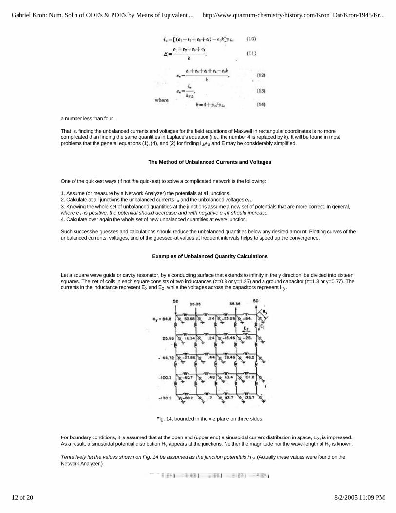
Let a square wave guide or cavity resonator, by a conducting surface that extends to infinity in the y direction, be divided into sixteensquares. The net of coils in each square consists of two inductances (z=0.8 or y=1.25) and a ground capacitor (z=1.3 or y=0.77). Thecurrents in the inductance represent Ex and Ez, while the voltages across the capacitors represent Hy.

Fig. 14, bounded in the x-z plane on three sides.

For boundary conditions, it is assumed that at the open end (upper end) a sinusoidal current distribution in space, Ex, is impressed. As a result, a sinusoidal potential distribution Hy appears at the junctions. Neither the magnitude nor the wave-length of Hy is known.

Tentatively let the values shown on Fig. 14 be assumed as the junction potentials H y. (Actually these values were found on theNetwork Analyzer.)


13 of 20 8/2/2005 11:09 PM

FIG. 15. Unbalanced currents and voltages on the wave guide network.

Figure 15 gives the unbalanced currents and voltages that will have to be liquidated. It should be noted that the greatest unbalancedjunction current is 7.93 amperes. As the greatest coil current is 102.8 amperes, that represents an 8 percent inaccuracy.

Knowing the unbalanced currents and voltages at every junction, a new set of junction potentials may now be assumed.

For an elastic stress problem of a beam, a set of junction potentials (representing displacements in the x or y directions) and a set ofunbalanced currents are shown in Fig. 16 (reproduced from Carter (8)).

The Method of Weighted Averages

Instead of attempting to reduce the unbalanced quantities simultaneously at all junctions, it is possible to reduce them at one junction ata time. Two such methods will be shown .

(1)The unbalanced current and voltage are reduced to zero at a junction without compensating at the neighboring junctions (themethod of weighted averages).(2) Each time the unbalancect current or voltage is reduced at a junction, the unbalanced quantities at the neighboring junctions arecompensated simultaneously (the relaxation method).

The first method is especially valuable when the guessed at value of potentials differs from the correct value only at isolated points orregions. Such is the case usually in Network Analyzer solutions when at some junctions the instrument reading is incorrect or the boardunit happened to be incorrectly set. The steps are as follows:

(1) Assume (or measure) the potentials at all junctions.(2) Calculate E, the weighted average, at any junction by Eq. (2).(3) Replace e0 by E.

In the previous method e0 was not replaced by E. Only the corresponding eu for each e0 was calculated, leaving e0 undisturbed.

It is customary to start at one corner of the network and change in succession all e0 to E, utilizing the already corrected potentials


14 of 20 8/2/2005 11:09 PM

wherever they are available. A disadvantage of this method is that it is equivalent to reducing the unbalanced potential eu at each junction immediately to zero.

A more advantageous procedure is to replace at each junction the value of e0 not by E but by a value larger than E, or smaller (depending on the value of the neighboring potentials) leaving thereby at each junction an unliquidated e u that is within the allowablelimit of error.

In non-linear problems it is often possible to plot curves which give outright the value of E for given neighboring potentials (or rather forgiven potential-differences between neighboring junctions). If difficulties in the convergçnce arise, in place of E a value larger (orsmaller) should be used.

The Relaxation Method

The relaxation method reduces the unbalanced currents or voltages at one junction at a time toward zero in a systematic manner. It isbased upon the fact that whenever the absolute potential of a particular junction is changed, the unbalanced currents and voltageschange only at that particular junction and at all the neighboring junctions to which a coil leads, while everywhere else the unbalancedjunction currents remain unchanged.

This fact may be seen by introducing a set of hypothetical generators so that (Fig. 17a):

(1) At every junction a generator with zero impedance is assumed to be connected to the ground. (2) The generator voltage is equal to the absolute potential of the junction. (3) The generator current to ground is equal the to unbalanced current existing at that junction.

By the introduction of these hypothetical generators the network remains unchanged and is now capable of performing new feats that itcouldn't do otherwise. Since the generators have zero impedance to ground, whenever one of the generator voltage is changed,currents can flow from this generator only to the neighboring grounds. (Fig. 17b). No change of currents exist anywhere else in thenetwork.

Hence, the unbalanced currents are reduced in two steps:

(1) Add (or subtract) a certain number of volts to the potential of a junction. (2) Find the new unbalanced currents (or voltages) at that junction and in the neighboring junctions.

Whether the unbalanced currents, or voltages, or both should be calculated depends on the problem at hand.

The "Unbalanced-Current Patterns"

The work involved in this last step may be greatly reduced in linear problems by the device of the "unbalanced-current pattern". Thisdevice consists of calculating once for all the change in the unbalanced junction currents caused by a change of one volt at every junction. (With nonlinear coils this device cannot be used.) Two cases may be distinguished:


15 of 20 8/2/2005 11:09 PM

(1) If the square nets of impedances throughout the network are identical, then each junction that does not lie on the boundary, hasidentical current-pattern. Similarly all horizontal, also all vertical, boundary junctions have identical pattern, as well as all corners. Thevarious patterns for the wave- guide example are given in Fig. 18 (plus current flows into a junction, minus current flows out of ajunction).(2) If the impedances vary from point to point, then for every junction a different current-pattern has to be established.

In analogy to the "unbalanced current patterns" it is possible to set up "unbalanced voltage patterns" by multiplying each iu by itsrespective Sy.

The Numerical Reduction

It should be noted that every time a junction- voltage is decreased, the junction currents at the neighboring junctions increase, but at thejunction itself it decreases. And the decrease is always greater than the increase (—4.23 amp. as against 1.25 amp.).

Hence the general procedure is to decrease (or increase) the unbalanced currents at those junctions where the unbalance is thegreatest. Two columns should be established at every junction:(1) One column showing the change in the absolute potential assumed. (2) The other showing the new unbalanced currents (or voltages, or both).

There will be many more entries in the current column since the current varies also whenever the potential at a neighboring junction varies.

Fig. 19. Reduction of unbalanced currents to one-half of their value (from 8 percent to 4 percent).

Fig. 19 shows the steps necessary to reduce in the example of Fig. 15 the unbalanced currents from 8 percent to 4 percent. By changing the voltages only at five junctions, the accuracy of the a.c. Network Analyzer results has been increased 100 percent.


16 of 20 8/2/2005 11:09 PM

Fig. 20. Reduction of unbalanced currents to one-fourth of their value (from 4 percent to 2 percent).

Figure 20 shows the steps necessary to reduce the unbalanved currents from 4 percent to 2 percent. Now 24 changes had to beassumed instead of five to increase the accuracy by another 100 percent. To reduce the unbalanced currents from 2 percent to 1percent probably the same or greater number of changes would be necessary.

It is emphasized that a practiced person could probably have made the same reduction by less than 24 steps. Also, the network issymmetrical, a fact which was not considered in the reduction.

No hard and fast rules can be established for the reduction. While it is possible to assume at a junction a change of potential thatreduces its own unbalanced current immediately to zero, it will not remain so as soon as the potential at a neighboring junction isassumed to vary. Often

it is advantageous to reduce an unbalanced current not only to zero but to a negative value.

Group Relaxation

There is no limit of course to the amount and type of labor-saving devices, that can be introduced. One of them will now be considered.

Instead of assuming a change of voltage at one junction, a change of voltage at several junctions may be assumed simultaneously.This requires settig up "current patterns" for several junctions. An example, for three border junctions is shown in Fig. 21.

FIG. 21. Current pattern for three border junction.

Networks with Complex Impedances

If both resistances and inductances occur in a network, then the unbalanced junction-currents are complex numbers i1+ji2, instead of real numbers i1. Similarly the absolute potentials are complex numbers. Then a separate current pattern has to be established for aunit change in the real and the imaginary components of junction-voltage respectively. The latter must so change that both the real andimaginary parts of unbalanced currents approach zero.

Another and perhaps a better method is to replace the equivalent circuit by a more complex circuit in which only real numbers occur.Such a step is always possible since a set of differential equations containing complex coefficients may always be replaced by a set


17 of 20 8/2/2005 11:09 PM

containing no j by simply doubling the number of equations and the number of dependent variables, that is, by introducing in-phase andout-of-phase components of variables.

The "Diffusion" Method

While the relaxation and the weighted average methods change potentials at one junction at a time, the method of unbalanced currentsand voltages changes the potentials at all junctions simultaneously. The first two methods are found to be effective at the beginning ofthe reduction, especially in the elimination of "bumps" in otherwise smooth curves; afterwards the latter method appears to be faster.When the unbalanced currents are small compared with the circuit currents but still further reduction is desired, all three methodsbecome very slow. The following method offers a further systematization of the third method.

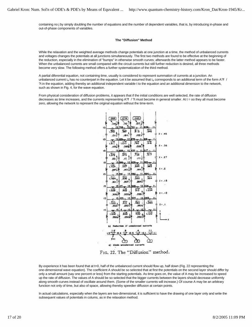
A partial diferential equation, not containing time, usually is considered to represent summation of currents at a junction. Anunbalanced current iu has no counterpart in the equation. Let it be assumed that iu corresponds to an additional term of the form A?f /?t in the equation, adding thereby an additional independent variable t to the equation and an additional dimension to the network,such as shown in Fig. 4, for the wave equation.

From physical consideration of diffusion problems, it appears that if the initial conditions are well selected, the rate of diffusiondecreases as time increases, and the currents representing A?f / ?t must become in general smaller. At t = oo they all must becomezero, allowing the network to represent the original equation without the time-term.

By experience it has been found that at t=0, half of the unbalanced current should flow up, half down (Fig. 22 representing theone-dimensional wave equation). The coefficient A should be so selected that at first the potentials on the second layer should differ byonly a small amount (say one percent or less) from the starting potentials. As time goes on, the value of A may be increased to speedup the rate of diffusion. The values of A should be so selected that the bigger currents between the layers should decrease uniformlyalong smooth-curves instead of oscillate around them. (Some of the smaller currents will increase.) Of course A may be an arbitraryfunction not only of time, but also of space, allowing thereby speedier diffusion at certain points.

In actual calculations, especially when the layers are two-dimensional, it is sufficient to have the drawing of one layer only and write thesubsequent values of potentials in colums, as in the relaxation method.


18 of 20 8/2/2005 11:09 PM

PART III. CHARACTERISTIC-VALUE PROBLEMS

Oscillatory Circuits

In characteristic-value problems not only the mode of vibration (the junction-potential

distribution) is unknown, but also the frequency ? corresponding to that mode. If, however, a potential distribution is assumed, thecorresponding ? may be found by the following property of the networks, a consequence of Rayleigh's Principle.

"When the network potentials correspond to a characteristic function, the algebraic sum of the positive and negative powers in theinductors and capacitors is zero."

That is, the power SI2XL = SE2YL = SEIL in the inductors is equal to the power SI2XC in the capacitors. Or the power in the variableunits, that are functions of ? , is equal to the power in the constant units. This zero power in the network is utilized in findingcharacteristic values with the aid of a Network Analyzer. The admittances of the coils that are functions of ? are varied with w until agenerator, connected in shunt with any of the coils, draws no current from the line. At such values of admittances, the network isself-supporting and the stored electrical energy oscillates between' the capacitors and the inductors.

Calculttion of Characteristic Values

Hence, for an assumed potential distribution e, the corresponding ? is found by the following steps:

1. Calculate the power SI2X in all the coils that are not functions of ? (positive power exists in inductors and negative in capacitors).,This power may also be found by calculating the power flowing in the coils that are functions of ? . If the latter are ground coils, then if eis the junction potential and i the current through the ground coils, power = Sei.

2. If the admittance of each of the remaining coils is the same and is equal to ? 2C, then the power in these coils is e2y = Se2? 2C =? 2CSe2. Hence

By Rayleigh's principle it is well known that if the assumed mode of vibration (potentials) is

only a rough approximation, the resultant characteristic value calculated is a better than rough approximation.

By knowing the correct ? for an assumed potential distribution, the correct unbalanced currents iu and eu may now be calculated. Thelatter in turn may be reduced by any of the four methods shown for the solution of boundary- value problems. However, in the presentproblems a new and more correct ? has to be calculated occasionally as the reduction proceeds.

The Method of Unbalanced Admittances

In the presence of coils that are functions of ? and whose admittances are usually equal, it is not necessary to introduce unbalancedcurrents. Instead the unbalance is redistributed by attributing different admittances to these variable coils. Hence when the correct ?has been calculated for a given potential distribution, it is assumed that with each variable coil an unbalanced admittance yu is associated. The purpose of the reduction is then to reduce the values of these unbalanced admittances.

Expressed in another way, the purpose of the reduction is to make the admittances of all variable coils the same. The calculated ?only gives a goal to aim at at the beginning. As the reduction proceeds, the common value of the admittances continuously shifts.


19 of 20 8/2/2005 11:09 PM

The use of the "unbalanced current patterns" facilitates the calculation of the unbalanced admittances at the neighboring points, whenthe potential at a point is changed.

Linear Harmonic Oscillator

It will be assumed that an approximate value of a characteristic function of the linear harmonic oscillator is known, Fig. 23. (Actually ithas been measured on a Network Analyzer, (9) with the aid of the network of Fig. 24.)

The problem is to calculate the corresponding characteristic value. Theoretically that is known to be yE=0.0880. zero generator currentat yE=0.0921, a 4 percent discrepancy.

The admittance of the horizontal inductors was Yh=1.1 and those of the vertical inductors yv=O.00704x2 where x varies from 1/2 to 12 1/2 in steps of 1 as given in Table I for half the coils. The measured potentials from ground to junction are given in Table II.

In the Schrödinger equation the admittance of the capacitors is proportional to ? . The energy in the horizontal coils is S1.1?e2 = 2851,

in the vertical coils it is fey, Se2yv = 2890. Hence

This calculated energy level differs from the theoretical value of 0.0880 by only 3 parts in 10,000. It should also be noted that the true(and lowest) energy level 0.0880 is always smaller than the approximate levels 0.0883 or 0.0921, in accordance with Rayleigh'sprinciple, or its quantum mechanical analogue.

Here ? is the approximate wave function e. Also H?x? is the current i in E?x the admittance yE.

BIBLIOGRAPHY

(1) H. W. Emmons, "Numerical methods of solving partial differential equations," Quart. App. Math. (Oct. 1944).

(2) A. Vazsonyi, "Numerical method in the theory of vibrating bodies", J. App. Phys. 15, 598 (1944)

(3) G. Kron, "Equivalent circuits of the elastic field," J. App. Mech. 11, 149-161 (1944).


20 of 20 8/2/2005 11:09 PM

(4) J.B.Scarborough, "Numerical Mathematical Analysis (Oxford University Press, 1930).

R. E. Doherty and E. Keller, Mathematics of Modern Engineering I (John Wiley & Sons, Inc, New York, 1936), p. 167.

(6) J. H. Bartlett, "The shaping of pole faces of the betatron," Phys. Rev. 63, 185 (1943).

(7) G. Kron, "Equivalent circuits of compressible and incompressible flow fields," scheduled to appear in J. Aer. Sci.

(8) G. K. Carter; "Numerical and network ~.nalyzer solutions of the equivalent circuits for the elastic field;" J. App. Mech.11,162—167 (1944).

(9) G. K. Carter. and G. Kron, "A.c. network analizer study of the Schrödinger equation," Phys. Rev. 67, 44 (1945).

(10) G. Kron, "Electric circuit models of the Schrödinger equation," Phys. Rev. 67, 39 (1945).

(11) G. Kron, "Equivalent circuit of the field equations of Maxwell," Proc. I. R. E., pp. 289 - 299 (May, 1944).

(12) R. V. Southwell, Relaxation Methods in Engineering Science (Oxford University Press, 1940).

(13) A. F. Prebus, I. Zlotowsky and G. Kron, "The application of network analysis to some electron optical problems," scheduled, toappear in Phys. Rev.

Home Index Up

http://www.quantum-chemistry-history.comCopyright © Oct. 03, 2003 by U. Anders, Ph.D.

e-mail Udo Anders : [email protected]

Last updated : Oct. 03, 2003 - 18:25 CET

gabriel kron: num. sol'n of ode's & pde's by means...

Documents