gains from distortions in congested city networks.faculty.arts.ubc.ca/ftrebbi/research/maps.pdf ·...
TRANSCRIPT
Gains From Distortions in Congested City Networks.
Francesco Trebbi and Matilde Bombardini�
November 2012
Abstract
This paper presents a model and an automated methodology for assessing gainsfrom network distortions in cities. Distortions arise from excluding tra¢ c along cer-tain routes. Distortions degrade network connectivity, but can be paradoxically usefulfor congestion amelioration. We show that such distortions are quantitatively large,increasingly pervasive in larger cities, and potentially very valuable. The results ulti-mately support the view that Braess�(1968) paradox is not just a theoretically inter-esting possibility, but a widespread feature of city road networks.
�University of British Columbia and National Bureau of Economic Research, [email protected]; Uni-versity of British Columbia and National Bureau of Economic Research, [email protected], respectively.The authors would like to thank Daron Acemoglu, Richard Arnott, Gilles Duranton, David Lucca, AndreaMattozzi, Tim Roughgarden, Jesse Shapiro, Ken Small, Adam Szeidl, Matthew Turner, and Erik Verhoeffor useful discussion and Luigi Guiso, Paola Sapienza and Luigi Zingales for sharing their historical data onItalian cities. Kareem Carr, Seyed Ali Madani zadeh, Isaac Laughlin, and Carlos Sánchez-Martínez providedoutstanding research assistance. Laughlin also contributed to the data description section. Financial supportfrom the Initiative on Global Markets at Chicago Booth is gratefully acknowledged. An earlier version ofthe paper circulated under the title �City Structure and Congestion Costs�.
I. Introduction
This paper o¤ers two main contributions. First, we present an empirical methodology
based on network theoretic foundations for studying the microstructure of city road networks.
Second, we �nd strong empirical relationships between population, network structure, and
congestion costs. These �ndings provide guidance in restricting the set of ambiguous theo-
retical predictions that we report.
Concerning the network structure, the paper shows that there is an intuitive, but over-
looked connection between the way city tra¢ c plans are organized and Braess�(1968) seminal
counterintuitive observation that reducing the number of links in a network may actually
ameliorate its equilibrium level of congestion1. City planners systematically close o¤ roads
and directions of �ow to abate congestion at the cost of lower network connectivity. By
any standard such approach is more frequently employed than congestion pricing and more
readily implementable than changes in the provision of lane kilometers for any type of roads.
The paper assesses the empirical prevalence of such distortions and binds their economic
value in transportation networks.
Congestion costs are economically large. The Texas Transportation Institute assesses
total congestion costs in the United States at $115 billion in 2009 (based on wasted time and
fuel, excluding the environmental externalities of the 3:9 billion gallons of wasted fuel), 58
percent of which stem from very large urban areas. Couture, Duranton and Turner (2012)
provide an even larger economic assessments ($141 billion in 2008). This motivates our
interest.
We model a city as a directed graph and describe the time delay of going through the
network (latency) as a function of the �ow of agents routing through its arrows. We de�ne a
(city) planner�s problem as �nding a subgraph minimizing the aggregate congestion costs of
1Braess (1968) presents an example of how an increase in the connectivity of a network (e.g. addinga new link) may increase total tra¢ c congestion in equilibrium. This counterintuitive result is commonlyreferred to as Braess�paradox. This paradoxical result occasionally also surfaces in other forms, such as the"fundamental law of road congestion" (i.e. increasing road supply does not ameliorate congestion levels).See Duranton and Turner (2011).
1
sel�shly-routing agents moving through the network. This matches the empirical regularity
that not all sites within a city are accessible by tra¢ c and that the accessible vertex set is
a very deliberate subset of the overall city network. We study the equilibrium properties of
such optimal subgraph. Within our framework, tra¢ c �ow restrictions in the subgraph (e.g.
one-way tra¢ c and other forms of path distortion) are a direct expression of Braess�paradox
in networks. In other words, tra¢ c restrictions are interpretable as pruning arrows from a
transportation network to abate latency.2
Placing theoretical structure on the data, we quantify the endogenous congestion-minimizing
distortions in city transit networks in a large sample of United States and Italian cities,
to show the increasing pervasiveness of distortions in larger cities and to place reasonable
bounds on their economic value. Importantly, all this is achieved sidestepping the need for
detailed micro tra¢ c and speed data (hundreds of millions of roads/time data points, often
noisily measured), a major obstacle for the empirical analysis of congestion beyond samples
of very limited representativeness.3 To this goal, we introduce a novel automated search al-
gorithm on a widely available Internet mapping application4. The algorithm �rst generates
source-target routes within the network and then samples from the empirically implemented
viable subgraph (i.e. the actual tra¢ c plan). For a large sample of US and Italian cities we
estimate the endogenous congestion-minimizing distortions of transit networks by comparing
restricted versus unrestricted routes within the city. An average US daily commute is made
about 10 percent longer in terms of its distance as a result of network pruning. We also
show empirically that, as population increases, cities display larger distortions within their
networks. To the best of our knowledge, these stylized facts are new.
From a theoretical standpoint, the paper is related to a growing computer science liter-
ature focused on ine¢ ciencies arising within sel�shly routing networks. Our model builds
heavily on the work of Roughgarden and Tardos (2002) and Roughgarden (2002), which in
2See Section 2 for further discussion.3For a critical discussion, see Fosgerau and Small (2010). The authors also present an application to
Danish freeways with (exceptionally) clean data.4Our application of choice is Google Maps, available at http://maps.google.com/.
2
turn leverages on the voluminous transportation science literature on tra¢ c equilibria stem-
ming from Wardrop (1952). Our contribution should not be seen as theoretical though, but
in tightly mapping such abstract models into data. The paper is related to the vast litera-
ture on Braess�paradox in networks5 and proposes one of its few applications to real road
networks in a large sample of cities. Indeed, the prevalence of Braess�paradox in transporta-
tion networks is neither theoretically obvious 6 nor one that has little economic implications,
given its potentially large economic value.
From an empirical standpoint, we follow the same path as Lucca and Trebbi (2009)
in presenting theoretically-grounded information retrieval algorithms from web sources de-
signed to quantify hard-to-measure concepts in an automated and undirected fashion. This
paper is related to a vast literature on agglomeration, spanning industrial organization, in-
ternational trade, urban geography, urban planning, regional science, and urban economics.
The number of important contributions in this area is too large for a comprehensive review
here. Fujita, Krugman, and Venables (1999) and Fujita and Thisse (2002) provide excel-
lent overviews of the economic geography literature, while Anas, Arnott, and Small (1998)
and Small and Verhoef (2007) provide accurate reviews of the economics of urban spatial
structure and transportation. More closely related is the economic literature on congestion
and hypercongestion costs (Dewees, 1977; Arnott and Small, 1994; Verhoef, 2001; Small and
Chu, 2003; Arnott, Rave and Schöb, 2005; Duranton and Turner, 2011; Couture, Duranton
and Turner, 2012) to which this paper contributes by presenting a model of urban networks
matched to micro data. The paper is also related to the literature on quantifying urban
network structure and sprawl.7 Relative to this line of research, mostly focused on entropy
and dispersion measures, our approach di¤ers in that we focus on endogenous distortions
imposed on the network structure. Our contribution to this literature is dual, as we present
5Bounding the pervasiveness of Braess paradox in networks is studied, among others, by Lin, Roughgar-den, and Tardos (2004) and Lin, Roughgarden, Tardos, and Walkover (2009).
6For a discussion see Frank (1981); Valiant and Roughgarden (2010); Chung and Young (2010).7Examples include Gordon, Kumar, and Richardson (1989), Tsai (2005), Xie and Levinson (2006), Burch-
�eld et al. (2006).
3
both new automated measures targeted at quantifying city structure and an algorithm which
substantially improves on the small scale limiting previous studies.8
The work is organized as follows. Section 2 presents a model describing the city and the
main theoretical results in terms of congestion and agglomeration costs. Section 3 shows
how to link the theoretical representation of the network and the empirical city structure.
Section 4 presents the mapping algorithm and data. Section 5 reports our main empirical
results. Section 6 concludes and discusses future applications.
II. Model
We model a city as a directed acyclic graph C = (V;A) with vertex set V , indicating sites
within the city, and arrow set A. The graph displays i = 1; :::; k source-target vertex pairs
si� ti and multiple paths through C connecting each pair. We do not impose restrictions on
C, so the model caters to monocentric or multicentric, sprawling or compact macro urban
structures. This particular network representation and the analysis for sel�sh-routing �ows
are due to Roughgarden and Tardos (2002) and Roughgarden (2002, 2006).
We assume that the city population, N , is located at the sources s1; :::; sk each with
subpopulation shares w1; :::; wk,P
iwi = 1.9 We do not focus on the endogenous spatial
equilibrium and take the location decision as predetermined. While theoretically possible to
relax this assumption, unavailability of systematic data on the value of targets ti for di¤erent
city population subgroups (necessary to compute payo¤s in location trade o¤) would make
any empirical validation unfeasible.
Our location assumption is realistic in the case of short-term considerations (hence, our
model could be considered complementary to long-run models of endogenous residential
choice) or in instances where location decisions are driven more by amenities at si (school
quality, local public goods, etc.) than by considerations on a speci�c commute si � ti. In8For instance, Youn, Gastner, and Jeong, (2008) present an empirical analysis of Braess paradox in a
limited sample of 246 roads in Boston, Massachusetts.9For tractability individuals do not locate on a non-source, non-sink vertex in the network.
4
this latter sense, Quinet and Vickerman (2004, p.50) conclude that �empirical studies shed
further light on the theoretical analyses in suggesting that transport constitutes an important
factor, but one which is far from the sole determinant, in the location decision of activities.�10
Let us de�ne ri the total tra¢ c traveling on si � ti, that is the expected number of
agents making the si� ti trip per time period11, the input tra¢ c vector �!r = [r1; :::; rk]0, andPi ri = r the total tra¢ c rate in C. For example, we may consider si being a residential
suburb, ti a location in the central business district of the city, and si � ti the commute to
work for ri individuals out of the total ni = wiN residing at si. De�ne pi the per period
probability that an individual in ni has to undertake trip si � ti.12 For tractability we will
assume that these events are independent across individuals, so that ri = pini > 0.13 Input
tra¢ c rates are taken as given in what follows, while Appendix B presents a generalization
of the model allowing endogenous tra¢ c demand �!r .
For given origin-destination pair si � ti, also called a commodity, we allow individuals
to sort through di¤erent paths connecting si and ti. Call �Ci the (non-empty) set of paths
connecting si and ti in C, and f� the �ow on path � 2 �Ci . De�ne �C = [i�Ci . A �ow
f : �C ! R+ is called feasible ifP
�2�Cif� = ri for all i. Let us indicate with fa the �ow on
arrow a 2 A, so that fa =P
�:a2� f�.
We assume that the time necessary to travel along arrow a is described by a latency
function la(fa) with la : R+ ! R+, nonnegative, non-decreasing, continuous, and semi-convex
in the tra¢ c �ow along arrow a.14 Non-decreasing and continuous latency functions la(:)
10For the case of highways, the FHWA states that �Recent empirical studies conducted in Ohio andNorth Carolina indicate that local patterns of population growth (measured at the Census Tract level) arenot highly correlated with increases in highway capacity.�See Hartgen, D.T. (2003a, 2003b).11For the following theoretical analysis a speci�c assumption for time interval length is not necessary.
However one can consider a day a reasonable reference period. In the empirical analysis, daily trips aresampled over one year periods.12See Arnott, De Palma, and Lindsey (1993) for a structural model were endogenous departure decisions are
modeled explicitly and Vickrey (1969) for an earlier seminal contribution. However, the network consideredby Arnott, De Palma, and Lindsey (1993) is stark, as it includes a two vertex graph with a single bottleneck.13For the following theoretical analysis this assumption is immaterial. For the empirical application the
linear dependence of tra¢ c rates on population within the network should be considered a special case. Wediscuss it within the empirical methodology section.14Semi-convexity is a weaker assumption than convexity, in particular if la(x) is semi-convex, then xla(x)
is convex.
5
are standard in the tra¢ c routing literature (Roughgarden, 2002) and convexity is routinely
employed in empirical analysis by the US Federal Highway Administration (FHWA) as well
as in the theoretical literature (e.g. ; Chen and Kempe, 2007; Acemoglu and Ozdaglar,
2007).
Given a network C, a tra¢ c rate through the network �!r and set of latency functions l, we
indicate the total latency costs of a �ow f in C as L(f) =P
a2A la(fa)fa =P
�2�C l�(f)f�,
where the latency on path � is l�(f) =P
a2� la (fa).
A. Optimal and Nash Flows
a. Optimal Flows For graph C, tra¢ c rate �!r , and latency functions l, Roughgarden
and Tardos (2002) de�ne a �ow f � that minimizes total network latency an optimal �ow.
Particularly, they show that an optimal �ow solves the following nonlinear program:
MinXa2A
la(fa)fa
s:t:X�2�i
f� = ri 8i(1)
fa =X
�2�:a2�f� 8a 2 A
f� � 0 8� 2 �C :
Under our assumptions on l, program (1) is convex and admits one feasible global optimum
f �. The minimum-latency �ow exists and is unique. We can think of f � as the solution that
a city planner able to fully and costlessly direct tra¢ c �ows through C would implement.
Intuition would suggest L (f �) be monotonically non-decreasing in tra¢ c rates, which
the following proposition con�rms.
propositionf f � and f �0 are feasible optimal �ows for (C;�!r ; l) and (C; (1 + )�!r ; l) re-
spectively, with > 0, then L (f �) � L (f �0).
Proof. In Appendix.
6
Note that in Proposition 1 (1 + )�!r indicates a scalar multiplication, that is we are
increasing proportionally tra¢ c inputs at every source si. Although restrictive, it will be-
come clear below that focusing on this type of tra¢ c increments substantially facilitates the
tractability of the analysis.
b. Nash Flows It is possible to extend the analysis to decentralized solutions, and char-
acterize the �ow f at a Nash equilibrium in the triple (C;�!r ; l) : Nash equilibria for this
problem are reasonable approximations to individual behavior in presence of atomistic, self-
ish agents endogenously routing through the network (Roughgarden, 2002). Such agents
fully incorporate in their decisions the latency of each arrow when choosing a path (picking
the minimum-latency path), but will not incorporate in their decisions the additional conges-
tion externality they bring to that speci�c �ow. In transportation science this is commonly
referred to as the Wardrop (1952) equilibrium problem for urban road networks.
de�nition�ow f is a Nash equilibrium �ow if and only if l�1 (f) � l�2 (f), for every �ow-
carrying path �1 2 �Ci and every path �2 2 �Ci , for every i = 1; :::; k.
If a �ow f is a feasible Nash �ow, then any two si� ti paths �1; �2 2 �Ci carrying positive
�ow must have the same latency l�1 (f) =P
a2�1 la(fa) = l�2 (f) = `i. This further implies
L(f) =P
i `iri.
Beckmann, McGuire, and Winsten (1956) and Roughgarden and Tardos (2002) show the
following existence and uniqueness result, whose proof we omit for brevity:
propositiononsider a triple (C;�!r ; l) with l continuous and non-decreasing: (a) (C;�!r ; l)
admits a feasible Nash equilibrium �ow f . (b) If f and �f are feasible Nash �ows, then
L(f) = L( �f):
For given triple (C;�!r ; l), a Nash �ow f will generally not achieve minimum latency,
that is L(f) � L(f �). Agents sel�shly routing through the network fail to incorporate the
negative externality they induce upon each other15. This results in the possibility of some
15For an early discussion see also Walters (1961).
7
counterintuitive outcomes in tra¢ c networks which we now explore.
We begin by deriving a useful monotonicity result for Nash �ows with respect to tra¢ c
inputs. We show that proportional tra¢ c increases in multicommodity networks (k � 1)
guarantee higher latency:
propositionf f and f 0 are feasible Nash �ows for (C;�!r ; l) and (C; (1 + )�!r ; l) respec-
tively, with > 0, then L(f) � L(f 0).
Proof. In Appendix.
The result that increased tra¢ c should increase total congestion at Nash equilibrium may
appear obvious, but it is not. To the contrary, equilibrium congestion may actually decrease
when the overall tra¢ c input in a network increases. Fisk (1979) provides an example where
a tra¢ c demand�s increase along one origin-destination (O-D) pair reduces total latency in
the network. Figure 1 modi�es such example allowing input tra¢ c increases in all O-D�s.
Total congestion falls in this case as well. The intuition behind this counterintuitive result
is that an increase in the overall tra¢ c input may not necessarily increase latency on a
speci�c edge. Indeed, there are instances in which the use of an edge is reduced when tra¢ c
input increases, as for edge (b; c) in Figure 1. General results for arbitrary vectors of tra¢ c
inputs�increments are thus not available, but some advancements have been made in the
literature. An increase in the tra¢ c input on an O-D, holding other inputs constant, is
proven to increase the latency of that speci�c origin-destination16, although positive changes
in demand in all O-Ds do not guarantee higher congestion. The reason why proportional
increases in demand are sure to induce monotonicity is based on the fact that, in general,
one can only prove that the average latency of an origin-destination pair weighted by its
change in demand is increasing (Dafermos and Nagurney, 1984). Proportional increases
guarantee that the average O-D latency weighted by the level of demand behaves in the
16Hall (1978) proves that, under some symmetry assumptions, each source to target latency `i is a monotonenondecreasing function of ri, for ri > 0, when all other tra¢ c rates rj , j = 1; 2; :::; k, j 6= i are held constant,using sensitivity analysis for convex programs. This result is extended to asymmetric cases in Dafermos andNagurney (1984). Lin, Roughgarden, Tardos, and Walkover (2009) prove a monotonicity result in a singlecommodity network (k = 1) using a direct combinatorial proof.
8

same way17. Proposition 3 should be viewed as providing a restrictive, but tractable case for
useful comparative statics18.
B. Optimal Network Design
For given triple (C;�!r ; l), a reasonable representation of a city planner�s problem is
unlikely to be well described by (1), due to the non-trivial costs of assigning agents to
speci�c routes in a directed fashion19 or to the cost of optimally taxing each speci�c edge
in the graph to internalize marginal social costs20. In practice, city planners aim at �nding
restrictions on accessible vertices that allow reductions in latency costs. More formally, the
problem is to �nd the subnetwork M of C, over which agents sel�shly route themselves,
displaying the lowest latency at Nash equilibrium. For given triple (C;�!r ; l), the problem
can be represented as the following network design program:
Min~M � C
fL(h)g(2)
s:t: �~Mi 6= ?; 8i
h is a feasible Nash �ow for�~M;�!r ; l
�
For every subgraph ~M with rate �!r and latency functions l there is a unique Nash �ow, hence
(2) admits a solution. However, �nding the minimum-latency subnetwork M in problem (2)
is NP-hard even in single commodity settings (i.e. with a single source-target pair), as
proven by Roughgarden (2006), the �rst to introduce this problem in theoretical Computer
Science.21 A solution M to (2) exists. In the remainder of this section and for our empirical
17The level of demand is what matters for total congestion comparison. It is precisely a little gain on ahigh-demand O-D that drives Fisk�s paradox for instance.18Other applications employing such type of proportional increases include Roughgarden (2002) and
Roughgarden and Tardos (2002) in their bicriteria results.19Randomizations based, for instance, on licence license plate numbers are not uncommon anti-congestion
policies used to direct �ows, but what we emphasize here is that the main instrument for congestion abate-ment available to city planners is based on restrictions on access to certain vertices of graph C.20See Walters (1961).21For linear latency functions Cole, Dodis, Roughgarden (2006) prove that taxes on arrows can also be used
to improve total latency in the network and they are equally e¢ cient as arrows�removal. For general latency
9

analysis we will assume that it is known to the planner.
As further discussed in the following section, our analysis will take city structure (C;�!r ; l)
as given and perform comparative statics on the optimal subnetwork mapM with respect to
N . In the empirical analysis we will discuss how the actual city structure can be represented
by (C;�!r ; l) and how the empirical transit restrictions approximate (M;�!r ; l).
A comment is in order here. The idea of decreasing aggregate latency by reducing the
number of available arrows within a network may appear prima facie counterintuitive. A
more connected network should guarantee lower congestion. However, this is not always the
case. Since Braess (1968) seminal work, a large literature has developed around this seem-
ingly counterintuitive result. Large negative social externalities can arise from decentralized
privately bene�cial actions. Improving the connectedness of the network may further in-
crease incentives towards privately bene�cial but socially costly actions and further decrease
aggregate e¢ ciency. Figure 2(a) illustrates an example of a triple (C; 1; l) displaying Braess�
paradox. In Figure 2(b) by removing arrow (v1; v2) one obtains an optimal subgraph (M; 1; l)
with lower Nash equilibrium latency.22
We now discuss some results concerning total latency costs in optimal subnetworks. Let us
�rst notice that, given city structure (C;�!r ; l), increasing the tra¢ c rate through the optimal
subnetwork M to a higher level �!r 0 = (1 + )�!r > �!r produces an increase in congestion,
that is L(h) � L(�h), where h and �h are feasible Nash �ows for (M;�!r ; l) and (M;�!r 0; l)
respectively. This statement follows directly from Proposition 3. More importantly, even
allowing reoptimization of the subnetwork for the new triple (C;�!r 0; l) is not su¢ cient to
reduce total latency, as proven by the following proposition.
propositionor tra¢ c rates �!r and �!r 0 = (1 + )�!r with > 0, let M and M 0 be the
optimal subgraphs for (C;�!r ; l) and (C;�!r 0; l) respectively. If h and h0 are feasible Nash
�ows for (M;�!r ; l) and (M 0;�!r 0; l) respectively and l satis�es strong monotonicity, then
functions, they prove that taxes are more powerful than arrows�removal. Empirically, arrows�removal andaccess restrictions are more common than taxes as mechanisms of congestion regulation in urban areas.22See Roughgarden (2006).
10
L(h) � L(h0).
Proof. In Appendix.
This monotonicity result shows that if the tra¢ c rate �!r going through the triple (C;�!r ; l)
increases, then total latency L(h) in the optimal subnetwork has to increase. This theoretical
result is novel, but much of its relevance comes from the empirical implications we derive in
what follows.
Under general assumptions on graph and latency other properties of the optimal subgraph
remain elusive. For instance, even for k = 1 and with strictly convex latency functions, L(h)�s
convexity with respect to�!r is not generally given23. Notice further that there is no assurance
ofM 0 �M , i.e. optimal subgraphs will display a progressive shedding of edges as population
grows. As a counterexample let us double tra¢ c input to r = 2 in Figure 2(b). We can show
that M 0 = C is an optimal subgraph for (C; 2; l), while for r = 1 the optimal subgraph M
was obtained by removing edge (v1; v2). This implies M �M 0.
III. Empirical Mapping
We now operationalize the model and show what are its useful insights in interpreting
the mapping data.
A. City Structure: Assumptions
We begin by giving the empirical correspondences of the network C = (V;A) and the
optimal subnetwork M . Sites within a city can be represented by a set of points on a map.
This corresponds to the vertex set V of C. Arrows A in the directed graph indicate the
direction of �ow allowed from vertex to vertex (or from site to site).
Directions of �ow are endogenous within cities and we represent such restrictions through
subgraphM , the solution to problem (2). With regard toM , a planner is allowed to restrict
23Hall (1978) p.214 reports a counter-example for strictly convex latency functions.
11

access to a subset of the vertex set V in order to minimize total latency. This matches quite
accurately the design of tra¢ c plans for urban automotive transit. In the rest of our analysis
we will focus on automotive tra¢ c for this reason and because a large share of movement
within a city is by ground transportation.
Our main operational assumption will be that planners intend to minimize latency as
a primary objective. Empirically, congestion mitigation commissions routinely implement
tra¢ c control plans restricting access to certain routes and allow tra¢ c �ows to self-route
through the remaining accessible edges of the graph to guarantee mobility over a given set
of routes fsi; tig i = 1; :::; k. We recognize, however, that city planners may also have other
goals in designing M : minimizing accidents, favoring some routes over others in the name
of city development or as the result of pork-barrel/NIMBY politics, etc. As long as these
secondary concerns do not completely trump tra¢ c control, our model should still display a
reasonable �t of the data.
City structure is described jointly by C and by the latency functions l.24 An arrow�s la-
tency is generally the result of historical design (think of the thick Medieval walls restricting
entry points to an Italian city center), but also of progressive reoptimization by transporta-
tion authorities. Certain roads are designed to carry a speci�c amount of �ow. In our
analysis we will consider latency functions l as given and control for historical and physical
constraints that may induce higher latency on speci�c edges. Notice, however, that while
we take latency functions l as exogenous, the �ows argument of the function (and hence the
latency) are endogenous in our setting.
Concerning travel demand elasticity, for every i, we are allowing perfect elasticity of
travel demand along each particular path �i in the network, combined with an inelastic travel
demand over the si� ti commodity. This assumption aligns with the FHWA statement that
�The magnitude of demand elasticity depends heavily on the scope and time frame over which
24We take the network structure as predetermined and operate by �nding optimal subnetworks. Theendogenization of network structures is a topic addressed by a growing literature within Economics. See forinstance Acemoglu, Bimpikis and Ozdaglar (2009) and Jackson (2005) for a survey. An empirical exampleof the analysis of endogenous city structure is Burch�eld et al. (2006).
12

travel demand is being measured. For example, a demand elasticity measured with respect
to a single facility includes trips diverted from other routes or time periods and would be
much higher than demand elasticities measured over a corridor or region.�25 It is important,
however, to assess how sensitive our theoretical results are to the relaxation of the commodity
i perfectly inelastic travel demand assumption. Appendix B presents a generalization of the
model to the case of elastic travel demand and discusses in detail how our main theoretical
implications are robust along this dimension.
Finally, a core innovation in our empirical mapping is to avoid the necessity of extensive
tra¢ c data information. Such micro information, albeit available for very limited areas, is
not systematically available for the very large cross section of cities we employ.26
B. Empirical Implementation
Tra¢ c �ows along the di¤erent arrows within a city can be mapped into equilibrium Nash
�ows. If a �ow f is feasible and Nash in (C;�!r ; l), then any two si � ti paths �Ci;1; �Ci;2 2 �Ciwhich carry �ow must have the same latency `Ci . The same has to be true for latency `
Mi
in the optimal subgraph M with respect to the feasible Nash �ow h in (M;�!r ; l). Total
latencies must further satisfy L(h) =P
i `Mi ri �
Pi `Ci ri = L(f).
For j = M;C and for each si � ti commute, we can decompose latency `ji = �ji�ji by
multiplying physical distance �ji and equilibrium unit travel time (inverse speed) �ji = 1=vji
for a path in �ji . Ideally, one would like to measure aggregate latency costs L(h) =P
i `Mi pini
and all the components of this sum (distance, speed, share of �ow from each residency
location, location population at source). We show in the data section that some of this
information is available for a sample of US cities (but not all of it) and employ it to test
Proposition 4.
Without loss of generality let us order the paths in �Ci and �Mi in terms of increasing
25See: http://www.fhwa.dot.gov/planning/itfaq.htm26A necessary drawback of this approach is that, without micro �ow data, empirical testing whether tra¢ c
is actually at a Nash equilibrium is not feasible. We will specify explicitly our operational assumptions inthe subsequent empirical analysis.
13
distance, so �ji =��ji;1; �
ji;2; :::
where �ji;1 � �
ji;2 � ::: and so on. We do not require �
ji;z to
carry �ow in equilibrium for z = 1; 2; :::, but if it does, then we write `ji = �ji;z�
ji;z.
Let us de�ne �i the linear distance between si and ti. Since M is a subgraph of C,
by the triangle inequality it must be that �i � �Ci;1 � �Mi;1 for any i. This is because �i
is the euclidean distance between source and target, while �Ci;1 is the shortest-distance path
through the network when all edges are accessible, and �nally �Mi;1 is the shortest-distance
path through the subnetwork M .
Finally, let us notice that �Mi;1 may correspond to a path �Mi;1 carrying no �ow in equilibrium
(for instance, because �Mi;1 latency even at zero �ow is extremely high). However, at least
one minimum-distance �ow-carrying path �Mi;X 2 �Mi exists, given that ri > 0 and �Mi 6= ?.
By de�nition �Mi;1 � �Mi;X , so for �Mi;X it must be that for any i:
(3) �i � �Ci;1 � �Mi;X :
Let �vi be the reference speed at zero �ow on �Mi;X , we also have1�vi�Mi;X � �Mi;X�Mi;X for each i.27
The interesting point here is that �i, �Ci;1, �
Mi;X have a direct empirical correspondence.
Given a fsi; tig address pair, automated mapping applications accessible over the Internet
(such as Google Maps, which we employ) output directions including �i as the euclidean
distance, �Ci;1 as the walking distance, and �Mi;X as the driving distance. Google Maps further
supplies a reference travel time 1�vi�Mi;X based on speed limits. These are close empirical
matches of our theoretical quantities.28 An example for Midtown Manhattan is presented in
27�vi is sometimes referred to as free-�ow speed or zero-�ow speed in the literature.28We choose maps.google.com out of available web mapping interfaces (such as MapQuest.com or
maps.yahoo.com) for its response speed. Concerning directions, the Google maps algorithm�s details areproprietary. However, the algorithm is a variant of Dijkstra�s (1959) algorithm, the fastest algorithm tosolve weighted-graphs problems with non-negative edges (precisely the type of problems allowed within ourgraph C = (V;A)). The algorithm starts from a source and computes the latency to all directly connectedvertices, where latencies are approximated by edge length (if the shortest route is considered) or by edgelength weighted by speed limit (if the fastest route is considered). The algorithm then moves onto thefollowing set of connected verteces, and so on and so forth, until the shortest path to the target is found.Standard paths are stored in the Google Maps�cache to speed up computation.Two caveats are in order here. First, while directions by car are operative in Google maps, walking
directions are beta (in the empirical section we have to discard some bad output due to this issue). Second,Google maps currently does not allow for a shortest/fastest direction choice, but the output likely balances
14
Figure 3.
It is feasible to sample a large set of possible commutes from city address books and collect
this information. Incidentally, as theoretically predicted, the data will con�rm inequality
(3), with only a very small number of bad exceptions due to heuristic approximations within
Google.29
We can now present our main empirical remarks.
Remark 1. An explicit test of Proposition 4 can be formulated as:
If M and M 0 are optimal subgraphs of problem (2) for triple (C;�!r ; l) and (C;�!r 0; l)
respectively, where r =Pk
i=1 piwiN and r0 =Pk
i=1 piwiN0, and if N < N 0, then
kXi=1
��Mi;X�
Mi;X
�piwiN �
kXi=1
��M
0
i;X0�M0
i;X0
�piwiN
0
(i.e. total latency increases).
Remark 2. Given the following four claims:
1. If N < N 0, per traveler latency increases
kXi=1
��Mi;X�
Mi;X
�piwi �
kXi=1
��M
0
i;X0�M0
i;X0
�piwi;
2. If N < N 0, total delay increases
kXi=1
�Mi;X
��Mi;X �
1
�vi
�piwiN �
kXi=1
�M0
i;X0
��M
0
i;X0 �1
�v0i
�piwiN
0;
the two. We include more details on the interface in the Data Section. For our analysis we assume that ifGoogle Maps gives a path as the driving directions output, there is �ow on that path and it is the shortest�ow-carrying path, �Mi;X . This matches the fact that Google does not output necessarily the shortest drivingpath �Mi;1 but puts some weight on speed as well.29See Data Section for details.
15

3. If N < N 0, per traveler delay increases
kXi=1
�Mi;X
��Mi;X �
1
�vi
�piwi �
kXi=1
�M0
i;X0
��M
0
i;X0 �1
�v0i
�piwi;
4. If N < N 0, average reference latency increases
kXi=1
��Mi;X
1
�vi
�piwi �
kXi=1
��M
0
i;X01
�v0i
�piwi;
two su¢ cient conditions for Remark 1 and Proposition 4 to hold are: (a) Claim 2 and
claim 4 jointly hold; (b) Claim 3 and claim 4 jointly hold.
In Section 5 we validate empirically claims 2-4. If claims 2 and 4 hold jointly, Remark 1
must hold, hence verifying Proposition 4.30 If claims 3 and 4 hold jointly, claim 1 must also
hold31 and Proposition 4 will hold a fortiori.32
Testing Remark 1 o¤ers evidence in support of Proposition 4, our main theoretical impli-
cation, but does not o¤er evidence on whether increases in total latency originate exclusively
from slowing down of tra¢ c or from city plans M allowing only longer paths through their
edges (hence increasing average distance traveled) or both. As shown in the previous section
there is no assurance M 0 � M in general, so an open empirical question is whether:
Remark 3. City networks satisfy the following two claims:
1. If N < N 0, average distance traveled increases
kXi=1
��Mi;X
�piwi �
kXi=1
��M
0
i;X0
�piwi;
30If claim 2 holds thenPk
i=1 �Mi;X
��Mi;X � 1
�vi
�piwiN �
Pki=1 �
M 0
i;X
��M
0
i;X � 1�v0i
�piwiN
0: It follows from
claim 4 that:Pki=1 �
Mi;X
��Mi;X � 1
�vi
�piwiN �
Pki=1 �
M 0
i;X
��M
0
i;X � 1�v0i
�piwiN
0 �Pk
i=1 �M 0
i;X
��M
0
i;X
�piwiN
0 �Pki=1 �
Mi;X
1�vipiwiN . Adding
Pki=1 �
Mi;X
1�vipiwiN to all elements of the inequality implies Remark 1.
31By adding claim 3 and claim 4.32Notice however that Proposition 4 does not imply claims in Remark 2, nor under general assumptions
on the directed graph C and latency functions l such claims will necessarily hold.
16
2. If N < N 0, average speed of transit decreases
kXi=1
�vMi;X
�piwi �
kXi=1
�vM
0
i;X0
�piwi;
where vMi;X = 1=�Mi;X .
A �nal step in the empirical mapping is required. Our comparative statics with respect
to population N holds graph C constant. Empirically, C evolves over time within a city and
di¤ers across cities. Our approach is to hold speci�c �rst order statics of the directed graph C
constant, in particular characteristics a¤ecting the location of sites within the city (e.g. water
basins and streams, wetlands, steep-sloped terrain, coastal position, latitude, longitude,
elevation and variation in elevation over the city surface, etc.) and graph tortuosity.33 This
approach is admittedly rough, but to the best of our knowledge the only one implementable
for general comparison across city networks.
Let us de�ne the average path tortuosity for graph C and latency functions l:
(4) t(C; l) =kXi=1
��Ci;1 ��i
�wi:
A low-t city is one where moving from origin to destination is on direct lines (think
of walking through downtown Chicago), as opposed to a high-t city where moving on a
O-D path is on winding lines (think of walking through downtown Siena). Tortuosity is
occasionally mathematically de�ned through an arc-chord ratio, which in our case would
deliver the measure T (C; l) =Pk
i=1
��Ci;1=�i
�wi. Tortuosity parsimoniously helps capturing
limitations in the availability of links within the network, and historical features of the city
structure.33As explicitly stated in Section 5.A, in order to saturate for potential nonlinearities a fourth order poly-
nomial in tortuosity, as de�ned in (4), a fourth order polynomial in population density, and state �xed e¤ectsare also employed to condition on C.
17
Analogously to (4), we can de�ne the average per path distortion an individual incurs
due to congestion for given triple (C;�!r ; l) and for M solving (2):
(5) d (C;�!r ; l) =kXi=1
��Mi;X � �Ci;1
�wi:
When positive, (5) emphasizes how latency minimization induces excess circuitousness into
the subnetwork. It provides an intuitive measure of the degree to which paths have to be
more roundabout in presence of congestion relative to a theoretical benchmark where an
individual is able to freely travel through the network alone. Since such distortions precisely
obey the logic of the Braess�paradox, we refer to them as Braess�distortions. An analogous
mean ratio for transit distortions is D (C;�!r ; l) =Pk
i=1
��Mi;X=�
Ci;1
�wi.
Claim 1 of Remark 3, if veri�ed, implies:
Remark 4. If M and M 0 are optimal subgraphs of problem (2) for triple (C;�!r ; l) and
(C;�!r 0; l) respectively, where r =Pk
i=1 piwiN and r0 =Pk
i=1 piwiN0 with N < N 0, thenPk
i=1
��Mi;X � �Ci;1
�wi �
Pki=1
��M
0
i;X0 � �Ci;1�wi (i.e. average travel distortion increases).
A useful result in assessing the economic importance of Braess distortions is that excess
circuitousness in the subnetwork bounds from below the gains in terms of speed of transit
that must accrue due to the restrictions implemented by the planner, or more formally:
corollaryiven triple (C;�!r ; l) with optimal subnetworkM , for each si�ti the ratio between
driving and walking distance �Mi;X=�Ci;1 is less or equal than v
Mi;X=v
Ci;1, the ratio between the
speed on the shortest driving path inM and the speed at which it would be possible to drive
on the shortest path in the unrestricted network C.
Proof. In Appendix.
If the average excess distortion measured in a city isPk
i=1
��Mi;X=�
Ci;1
�wi = 1:1, this
corollary implies that tra¢ c moves on average at least 10 percent faster in the restricted
18
network relative to what would emerge in equilibrium in the (counterfactual) unrestricted
network.
IV. Data
A. Latency Costs
From the 2009 Annual Urban Mobility Report published by the Texas Transportation
Institute (TTI), part of the Texas A&M University System, we collect data on city-level to-
tal delayPk
i=1 �Mi;X
��Mi;X � 1
�vi
�piwiN , average delay per traveler
Pki=1 �
Mi;X
��Mi;X � 1
�vi
�piwi,
and average tra¢ c speedPk
i=1
�vMi;X
�piwi measures. Unfortunately, total latency is not
reported by TTI (2009a). The Annual Urban Mobility Report assesses time delays and
roadway congestion costs data for 90 large urban areas in the United States.34 Measures of
urban roadway congestion are generated from raw data on urban arterial and freeway tra¢ c
supplied through the Highway Performance Monitoring System from the Federal Highway
Administration. To the best of our knowledge, TTI�s Annual Urban Mobility Report is
among the most comprehensive and complete sources of congestion costs estimates available
for any country and the most comprehensive in terms of road miles covered for US cities.
For cross-validation purposes and robustness to employing tra¢ c data obtained from al-
ternative methodologies, we also collect congestion rankings from the INRIX National Tra¢ c
Scoreboard. INRIX, one of the country�s leading tra¢ c and navigation services company,
gathers and analyses raw data originated from its proprietary Smart Driver Network, includ-
ing 1:6 million GPS-equipped probe vehicles (including taxis, shuttle vans, service delivery
trucks, and consumer vehicles) generating speed, direction, and location information for the
largest 100 metropolitan areas in the United States.35
34See http://mobility.tamu.edu/ums/congestion_data/. The Annual Mobility Report includes estimatesof congestion costs for an aggregate of 439 urban areas. TTI however collects detailed data only on theoriginal 90 areas.The remaining 349 areas are rolled into 1 aggregate, in essence treating them as a single large urban area
for analysis purposes and no disaggregated data exist. We thank David Schrank at TTI for clarifying thisissue.35See http://www.inrix.com/pressrelease.asp?ID=94
19
Table 1 reports the top ten metropolitan areas for congestion costs in both samples. The
TTI and INRIX samples refer to tra¢ c conditions in the most recent period available (2007
and 2009, respectively), for maximal comparability between congestion costs and the corre-
sponding tra¢ c path distortions generated by the (continuously updated) Internet mapping
applications described below.
B. Braess�Distortions and Tortuosity
The process of measuring tra¢ c path distortions within the city network C is a crucial
methodological step in our analysis. Given the relative novelty of our approach we feel that
extra scrutiny is necessary. We do not limit ourselves to the analysis of US urban areas for
which TTI measures are available, but we extend the sample both cross-sectionally within
the United States and cross-country, focusing on Italian cities, an arguably di¤erent sample
in terms of urban structure and local administration organization.
Concerning US cities, we consider the top 500 most populous census designated places
(CDP). These data are available from the US Census Bureau36, which describes CDPs as
�delineated to provide data for settled concentrations of population that are identi�able
by name but are not legally incorporated under the laws of the state in which they are
located.�37
For the Italian city sampling we employ the cities considered in Guiso, Sapienza and
Zingales (2008), a large cross-sectional study of Italian municipalities. The data includes
INRIX coverage is more limited relative to TTI, as only mainline lanes of limited access highways areincluded in the INRIX samples.36The census places come from the 2000 vintage census data. Places in Puerto Rico are not considered in
constructing this list. U.S. Census Bureau. Places, cartographic boundary �les, descriptions and metadataare available at http://www.census.gov/geo/www/cob/pl metadata.html#cdp 200537Census designated places mostly conform to commonly recognized political boundaries, but there are
several results of this worth mentioning. Minneapolis and St. Paul, Minnesota for example, are consideredas two distinct CDP�s, not a single metro area. In some cases (e.g. Sarasota and Bradenton, Florida)cities which in tandem constitute a large metro-area, do not individually fall in the top 500 CDP�s andso are not considered in this analysis. Some CDP�s do not exist in any commonly understood sense, likeParadise, NV, which includes much of downtown Las Vegas, and exists for practical purposes, only as aCDP. These limitations and additional heuristics in Google (described below) limit the full U.S. sample to457 municipalities.
20
692 Italian municipalities and all Italian main urban areas (Capoluoghi di Provincia).
a. Path Sampling Population is located at C�s sources si and travels towards C�s sinks
ti. In order to generate a sizeable set of random commutes within a city we generate fsi; tig
i = 1; :::; k address pairs using a parallel algorithm for the US and Italian samples.
According to our model, source addresses can be randomly sampled, but sampling should
be weighted by source population. Consider collecting the addresses of all people called Smith
living in Chicago (or Rossi, living in Florence). Let us assume that people called Smith locate
at the sources s1; :::; sk with probability equal to the sources�subpopulation shares w1; :::; wk,
where wi = niNand
Piwi = 1. That is, we assume that a more populous suburb si has more
people called Smith than a less populous suburb si0 with wi0 < wi and that the share of
people named Smith is the same in both si and si0. Then, the distribution of people named
Smith is going to mimic the empirical distribution of source population s1; :::; sk and the
list of their addresses will provide a representative subset of source locations. Considering a
comprehensive list of last names further eliminates name-speci�c idiosyncrasies. We follow
this approach.38
The top 100 most common surnames in the US are derived using the available Census
(2009) totals for name frequency. The analog for the Italian version is based on data found
on the website cognomix.it. For each place, and each surname calculated above, addresses
are collected from phone directories.39 These addresses are then randomly paired in order
to create the endpoints for random routes through the city.
Notice that our path sampling approach focuses on residence-to-residence, not on residence-
38One caveat is in order. Our approach will not adequately capture city segregation by race in the case ofhighly race-speci�c last names. In particular, for racial minorities living in concentrated areas, names willnot appear random across network sources s. This may be relevant for Asian or Hispanic or Middle-Easternenclaves. Such distortions should be quantitatively small, however, and con�ned to a minority of the citypopulation.39We employed whitepages.com or paginebianche.it websites, for the U.S.or Italy respectively.Census designated places that do not conform to normal political boundaries may not have entries in the
white pages. In the top 500 most populous CDPs there are three that fail to return results from the whitepages. They are: Arden-Arcade, CA; Paradise, NV and Sunrise Manor, NV.In the Italian case it is possible to collect all data available, while from whitepages.com it is possible to
collect at most 100 addresses per name-place pair.
21
to-business pairs, which are more representative of a typical work commute (but not nec-
essarily of all trips within the city). Since residence-to-residence paths can cross business
districts, these structural features will not be lost in our data. For instance, in a circular
city model with residences uniformly located on a circumference of radius � and a central
business district of radius �=2 (hence, covering 1=4 of the city disk) the probability of any
random commute passing through the business district is 1=3. 40
For each city C, k is su¢ ciently large to guarantee asymptotic convergence of sam-
ple moments, such as d (C;�!r ; l) =Pk
i=1
��Mi;X � �Ci;1
�wi, to population moments, such as
d (C;�!r ; l).41
Finally, since estimates of pi are not generally available, in computing per traveler city
averages based on Google we will proceed under the assumption of a constant share of
travelers out of each location (i.e. constant probabilities pi = p). This will allow to focus on
all the empirical implications of the model, albeit at a cost in terms of generality.
b. Google Maps Data Once random commutes fsi; tig are generated, the various travel
distances between the points must be calculated. This is accomplished using the Google
Maps API, through which we can programmatically query the Google Maps service and
determine the travel distance by car, �Mi;X , and by foot, �Ci;1, for each commute. Figure
3 presents an example of a commute in Midtown Manhattan, where the driving distance
clearly exceeds the walking distance due to the speci�c restrictions of �ow along some of the
40The potential di¤erence in the distribution of business and residence locations can also be addresseddirectly by picking target destinations from business directories. We experimented with spot sampling fromWhite and Yellow Pages in a subset of U.S. cities without any evidence of systematic distortions in the data.We ultimately decided against the use of Yellow Pages because of the di¢ culty in systematically weighting�employment per business phone number�, a necessary component in assessing the likelihood of a givenbusiness commute (e.g. a large employer will be the target of more commutes than a small one, but theymay have the same number of phone numbers listed, as the large employer may only list its main number).41In the Italian data the number of pairs generated is a truncated function of the population of the Italian
census place. For census places with populations in the lowest or highest quartile, 0:5 percent of the relevantquartile boundary is used as the target number of pairs to generate. For census places with populations inthe interquartile interval, the number of pairs generated is equal to 0:5 percent of the actual population. Inthe US sample, 0:5 percent of the population of the 75th percentile city is used for all cities where enoughaddresses are available. This results in k = 622 pairs for each US city, unless the number of addressescollected is less than this total.
22

graph�s arrows. We also collected the latitude and longitude of the points in question, which
allows us to calculate the euclidean distance �i, between the points as well.42 This process
relies on the ability of Google to translate the given addresses into latitude and longitude
coordinates via a process called geocoding.43
In this project, each pair of points required two requests to the API, one to get the
distance based on driving directions, and one to get the distance based on walking directions.
From these requests, the travel distance, latitude and longitude, and the accuracy of the
location for both points were parsed from the JSON response and stored in a new data set.
Aggregate measures of these values, calculated for each census place, constitute the �nal
output of the procedure. The following items are constructed for each census place: 1. The
mean value of driving distance traveled; 2. The mean travel duration at reference speed; 3.
The mean value of the di¤erence between driving and walking distances d (C;�!r ; l); 4. The
mean value of the di¤erence between walking and euclidean distances t(C; l); 5. The mean
value of the ratio of walking to euclidean distances D (C;�!r ; l); and 6. The mean value of
the ratio of driving to walking distances T (C; l). For robustness checks we constructed all
the corresponding medians as well.
Some summary information about the data collection per city and its outcomes are
presented in Table 2. Much more data was collected for the US case than for the Italian case
when employing googlemaps.com. Reasons for di¤erences in the number of pairs attempted
and the number realized are: 1. Failure to properly geocode the address with high enough
accuracy. The Google Maps API returns a code indicating the accuracy of the mapping, we
accept values whose accuracy is indicated to be street-level or higher. 2. The Google Maps
API returns a code indicating failure to generate directions for the given points. Naturally,
such points have nothing to contribute to our analysis. 3. Paired addresses map to the same
42The euclidean distance is calculated using the Haversine Formula, which is a formula for calculatingshortest distances on a spherical approximation of the earth. It does not take into account changes inelevation.43The Google Maps API is fully described in that service�s documentation at google.com, and those
interested in the details of using the service are advised to look there.
23
location, resulting in zero distance for all measures. Such results are dropped.
As Table 2 also shows, the rate of failures in the Italian data is about three times that
of the US data. This is likely due to the relative di¢ culty of geocoding Italian addresses, to
the small size of some of the Italian cities in our sample, and poorer mapping information
for Italian cities.
Table 3 presents the summary statistics for both the TTI US sample and the full US
city sample. Units for distances are meters. On average the typical sampled path is 14:5 km
in driving distance in the TTI sample and 10:2 km in linear distance, reasonable commute
lengths. Delays�units are measured in annual excess hours, while travel duration at reference
speed (approximated speed limits) are reported in seconds. Tra¢ c congestion on average
produces 31 hours of delay per year per traveler (including cost of time and fuel the TTI
economic losses are substantial, as evident in the congestion cost estimates reported in the
Table). The average time duration of the typical commute at reference speed is about 16:5
minutes (990 seconds). This seems a reasonably representative �gure if compared with the
US Census 2009 American Community Survey average daily time to work of 25:1 minutes
(computed at actual speed). Finally, notice that both driving/walking and walking/linear
distance ratios are on average larger than 1, as required by (3).
V. Empirical Results
A. Remark 1: The Evidence
Lacking data on total latency, it is not feasible to test the main implication of the model
(Proposition 4) directly. In this section we follow an indirect approach.
We begin by showing that larger city populations N are positively correlated with longer
total delays (Remark 2, claim 2), longer delays per traveler (Remark 2, claim 3), higher
average reference travel durations (Remark 2, claim 4), longer average distance traveled
(Remark 3, claim 1), and lower average speed (Remark 3, claim 2). These �ve claims are
directly testable using either TTI data or Google Maps data. We present both uncondi-
24

tional and conditional scatterplots in Figure 4 to Figure 8. The set of controls for the
conditional regressions in the right panels includes: state �xed e¤ects (hence elasticities are
estimated employing within-state variation only), a fourth order polynomial in tortuosity
t(C; l), a fourth order polynomial in population density (a typical control for city structure),
a coastal city dummy, latitude, longitude, km2 of lakes/swamps/ocean, km of coast, km of
rivers/streams, mean elevation, standard deviation of elevation, mean terrain slope, standard
deviation of slope, percent area suitable for development44.
In all reported regressions we cluster our standard errors at the state level. All variables
are expressed in natural logarithms, to reduce the incidence of outliers.
Figures 4-8 make clear that claims 2-5 of Remark 2 and 1-2 of Remark 3 are all strongly
supported by the data. All regressions, unconditional and conditional, are statistically signif-
icant at standard con�dence levels. The unconditional elasticity of total delay to population
is estimated at 1:10. The unconditional elasticity of delay per traveler to population is
estimated at 0:34. The unconditional elasticity of travel duration at reference speed to pop-
ulation is estimated at 0:13. The unconditional elasticity of distance traveled to population
is estimated at 0:22. The unconditional elasticity of travel speed to population is estimated
at �0:08.
Figure 9 also reports scatterplots comparing TTI to the Couture, Duranton, and Turner
(CDT, 2012) and INRIX congestion indexes and population, a reduced-form result without
a direct link to our model, but reassuring of TTI data�s reliability. In particular, the CDT
inverse travel speed index is reassuring, as based on observed travel speeds by a sample
of commercial and privately owned vehicles from the National Household Transportation
Survey.
In order to test Remark 1 (i.e. Proposition 4) and claim 1 of Remark 2 we apply a
conservative multiple hypothesis testing approach based on the Bonferroni inequality (Savin,
1984). This is necessary as we are jointly testing multiple one-sided claims. For each null
44See Appendix C for variable de�nition and data sources.
25
hypothesis (i.e. that population elasticities of total delay, per traveler delay, and reference
travel duration are nonpositive), the Bonferroni correction requires the respective p-values to
fall below �=q, where � is the con�dence level and q = 3 is the number of multiple hypotheses
jointly considered (Remark 2, claims 2-4). We report the relevant one-sided hypothesis �2
test statistics and their p-values (both unconditional and conditional) in Table 4. We reject
each null hypothesis substantially below the :0033 (= :01=3) con�dence threshold with the
sole exception of the unconditional �2 statistic for reference travel duration, which has a
p-value of 0:0077. According to the Bonferroni inequality we reject the null that Proposition
4 fails at 5 percent con�dence level for the unconditional model and at 1 percent for the
conditional model. Claim 1 of Remark 2 is supported at equal levels of statistical signi�cance.
B. Remark 4: Braess�Distortions
Our model is predicated upon the assumption that city planners may restrict access to
network edges with the objective of minimizing total latency at Nash equilibrium. Under
general assumptions the model is silent on how increases in tra¢ c rates a¤ect the optimalM
(a task requiring far more stringent assumptions on the triple (C;�!r ; l)). However, we are
able to present direct empirical evidence on how population correlates with the average path
distortion d (C;�!r ; l) that an individual incurs due to congestion and show that Remark 4
holds in the data.
Figure 10 reports that larger city populations N are positively correlated with larger
Braess�distortions in the TTI sample, both conditionally and unconditionally. The uncon-
ditional elasticity of travel distortion to population is estimated at 0:37. Relative to Figure
7, where the estimated elasticity was 0:22, this result is quantitatively larger, re�ecting the
improvement in holding city structure C constant across cities when focusing on deviations
relative to the shortest path available �Ci;1.
Figure 11 shows that the positive relationship between Braess�distortions and city size
holds in the full US sample as well, and not just in the more limited TTI sample. Figure
26

12 presents kernel densities estimated for the overall sample of US cities. For completeness
we report here both average excess driving to walking distance d (C;�!r ; l) and average ratio
D (C;�!r ; l). For both measures Figure 12 highlights a relatively high dispersion in terms of
transit distortions across cities and heavily right-skewed distributions.
Moving to the Italian sample, Figure 13 again reports a positive and robust correlation
between path distortions and city population. Standard errors in all regressions are clustered
at the provincial level for the Italian sample.
The unconditional population elasticities range between 0:63 for the full US sample and
0:39 for the Italian sample, quantitatively comparable estimates. The quantitative implica-
tion in the most comprehensive US sample is that an extra 10 percent population moving
through the same city network is associated with an increase in the distance one has to
travel by car of an additional 6:3 percent. Going from A to B, where A and B are located
on average 6:7 km from one another, where the measure of distance is the euclidean distance
and where initial travel distortion is 1:78 km, requires 112 (= 1; 780 � 0:063) extra meters of
travel when the city population moving through the network increases by 10 percent.
To the best of our knowledge this represents a novel fact in the analysis of urban struc-
ture and one that points to a pervasive presence of Braess�distortions in more populated
networks. In addition, this fact has an interesting correspondence to a related literature
on the theoretical pervasiveness of the Braess�paradox in networks (Frank, 1981; Fisk and
Pallottino, 1981; Valiant and Roughgarden, 2010; Chung and Young, 2010).
C. Binding the Gains from Braess�Distortions in Cities
It is important to assess howmuch one can possibly gain from imposing Braess�distortions
in cities. For a �ow f feasible and Nash in (C;�!r ; l), Roughgarden and Tardos (2002) de�ne
the Braess�ratio as:
(6) �(C;�!r ; l) = max~M�C
"k
mini=1
`Ci
`~Mi
#.
27

Intuitively, the Braess�ratio indicates the largest congestion amelioration that can be ob-
tained by excluding some edges of graph C. A sizeable literature has developed around
placing theoretical bounds around Braess�ratios, including Lin, Roughgarden, Tardos, and
Walkover (2009) among the others. In this section we take a complementary route and
present empirical bounds for the value of Braess�ratio in cities.
It is unfeasible to focus on all possible tra¢ c plans for all cities in our sample as required
by (6), so we focus on the implemented M , modifying the de�nition of Braess ratio to:
(7) � (C;�!r ; l) =k
mini=1
`Ci`Mi.
Notice that when k = 1 then � (C;�!r ; l) = L(f)=L(h). Re-expressing total latencies in terms
of average distance and speed, we can bound the Braess�ratio:
� (C;�!r ; l) =�Ci;X�
Ci;X
�Mi;X�Mi;X
��Ci;X�
Ci;X
�Mi;X1�vi
��Ci;1�
Ci;1
�Mi;X1�vi
��Ci;1
1v0i
�Mi;X1�vi
,
where i is the path satisfying (7) and v0i the slowest speed on the shortest path in �Ci .
Google Maps allows to operationalize the upper bound by providing measures of �Ci;1
and �Mi;X . TTI calibrates a set of plausible approximations for �v=v0 in congested arterial
and freeway tra¢ c at heavy (�v=v0 = 1:21), severe (�v=v0 = 1:33), and extreme conditions
(�v=v0 = 1:51)45. These calibrations are necessary, as we do not observe the counterfactual
speed in the unrestricted network C. Assuming �v=v0 on all arrows, we could potentially
focus on the sampledk
mini=1
h�vv0
�Ci;1�Mi;X
ifor each city for consistency with Roughgarden and Tardos
(2002). However, a statistical approach more robust to idiosyncratic bad searches is to focus
on sample means of walk-drive ratios �vv0
Pki=1
��Ci;1=�
Mi;X
�wi.
For the US sample,Pk
i=1
��Ci;1=�
Mi;X
�wi = :92 implies an upper bound on the Braess�
ratio for that city of 1:11 in heavy conditions, or a gain of at most 11 percent from imposing
45Exhibit A-6. Daily Tra¢ c Volume per Lane and Speed Estimating Used in Delay Calculation in TTI(2009b).
28
Braess�distortions. Similarly we assess a 22 percent gain in severe conditions, and 39 percent
gain in extreme counterfactual conditions.
According to the Federal Highway Administration 2010 Tra¢ c Volume Trends, in the US
3; 000 billion miles were driven annually in 2009, about 60% of which were driven in urban
areas. This implies 1800 billion urban miles. Assuming a (conservatively high) average speed
of 40 miles per hour (coinciding with the TTI highway and freeway estimated average speed),
a value of time of $16:01 per person-hour and $105:67 per truck-hour as per TTI (2009a),
and assuming 95% of urban hours are driven by car, this implies a total urban latency of
$922 billion. It follows an upper bound on the economic value of Braess�distortions of $103
billion assuming heavy conditions in the counterfactual network, of $204 billion assuming
severe conditions, and of $360 billion in the extreme case.
While this exercise is not useful in assessing potentially informative lower bounds on the
value of such distortions (impossible to obtain without further assumptions on the counter-
factual equilibrium at C), it emphasizes under reasonable calibrations the potential of large
gains stemming from Braess�distortions.
VI. Conclusions
This paper o¤ers a contribution to the analysis of congestion costs in cities. We present
a theoretical model of congestion costs and endogenous tra¢ c distortions that allows a
straightforward mapping into empirically measurable quantities for a large sample of United
States and Italian cities.
We make use of widely available Internet mapping applications, verify the general predic-
tions of our model in the data, and further estimate positive and large population elasticities
of tra¢ c distortions in cities. We show that our results hold tightly across samples of large
and small cities within the United States and within a large sample of Italian cities. This
ultimately provides a novel set of cross-city stylized facts useful in the analysis of congestion
costs. We further interpret these �ndings as pointing in the direction of a large role for
29

Braess�paradox in more populated city networks. From a methodological standpoint, our
empirical path distortion and path tortuosity measures for cities can be considered useful
summary statistics of network structures, possibly of use to geography and transportation
economists.
Finally, one can further envision settings where network structure a¤ects the matching,
search, and interaction of individuals within the urban community. This is a relatively
di¢ cult problem to tackle quantitatively in Economics and in Sociology, but one for which
we o¤er a methodological addition. This suggests potential applications of our city network
measures, ranging from the analysis of social and cultural capital accumulation within cities
(e.g. Are cities with more di¢ cult/distorted city networks characterized by lower or higher
levels of social capital?) to the study of within-city location decisions of businesses.
30
REFERENCES
[1] Acemoglu, Daron, Kostas Bimpikis, and Asu Ozdaglar, 2009. �Price and Ca-pacity Competition,�Games and Economic Behavior, vol. 66, no. 1, 1-26.
[2] Acemoglu, Daron and Asu Ozdaglar, 2007. �Competition in Parallel-Serial Net-works� IEEE Journal of Special Areas of Communication, Special Issue on Non-Cooperative Behavior in Networking 25, pp. 1180-1192.
[3] Anas, Alex, Richard Arnott and Kenneth A. Small, 1998. �Urban Spatial Struc-ture�Journal of Economic Literature, 36, 1426-1464.
[4] Arnott, Richard, Andre de Palma and Robin Lindsey, 1993. �A StructuralModel of Peak-Period Congestion: A Tra¢ c Bottleneck with Elastic Demand�, Ameri-can Economic Review, 83, 161-179.
[5] Arnott, Richard and Kenneth A. Small, 1994. �The economics of tra¢ c conges-tion.�American Scientist 82: 446-455.
[6] Arnott, Richard, Tilmann Rave and Ronnie Schöb, 2005. Alleviating UrbanTra¢ c Congestion. MIT Press.
[7] Beckmann, Martin, C. Bartlett McGuire and Christopher B. Winsten, 1956.Studies in the Economics of Transportation. Yale University Press.
[8] Braess, Dietrich, 1968. �Über ein Paradoxon aus de Verkehrsplanung� Un-ternehmensforschung, 12, 258-268.
[9] Burch�eld, Marcy, Henry Overman, Diego Puga and Matthew Turner, 2006.�Causes of Sprawl: A Portrait from Space�, Quarterly Journal of Economics 121(2), .
[10] Census Bureau US, 2009.Genealogy data: Frequently occurring surnames from census2000 - US Census Bureau, December 29, 2009.
[11] Chen, Po-An and David Kempe, 2008, �Altruism, Sel�shness, and Spite in Tra¢ cRouting.�Proceedings of ACM EC 2008, Chicago, IL
[12] Chung, Fan and Stephen J. Young, 2010, �Braess�s Paradox in Large SparseGraphs�WINE.
[13] Cole, Richard, Yevgeniy Dodis and Tim Roughgarden, 2006. �How much cantaxes help sel�sh routing?�, Journal of Computer and System Sciences, 72(3), 444-467.
[14] Couture, Victor, Gilles Duranton, and Matt Turner, 2012 �Speed�, mimeo,University of Toronto.
[15] Dafermos, Stella and Anna Nagurney, 1984. �Sensitivity analysis for the asym-metric network equilibrium problem�. Mathematical Programming, 28:174�184.
31
[16] Dijkstra, Edsger, 1959. �A Note on Two Problems in Connection with Graphs�Nu-merische Matematik 1: 269:271.
[17] Dewees, Donald N., 1979. �Estimating the time costs of highway congestion.�Econo-metrica 47: 1499-1512.
[18] Duranton, Gilles and Matt Turner, 2011 �The Fundamental Law of Road Conges-tion: Evidence from US Cities�, American Economic Review, 101(6), 2616-52.
[19] Fisk Caroline, 1979. �More paradoxes in the equilibrium assignment problem�, Trans-portation Research 13B, 305-309.
[20] Fisk Caroline and S. Pallottino, 1981. Empirical evidence for equilibrium paradoxeswith implications for optimal planning strategies. Transportation Research, A15(3):245-248.
[21] Frank, Marguerite, 1981. �The Braess Paradox�Mathematical Programming 20: 283-302.
[22] Fujita, Masahisa, Paul R Krugman, and Anthony Venables, 1999, The SpatialEconomy: Cities, Regions and International Trade, MIT Press.
[23] Fujita, Masahisa and Jacques-Francois Thisse, 2002, Economics of Agglomera-tion: Cities, Industrial Location and Regional Growth, Cambridge University Press.
[24] Gordon, Peter, Ajay Kumar, and Harry W. Richardson, 1989. �The In�uenceof Metropolitan Spatial Structure on Commuting Time�Journal of Urban Economics,26, 138-151.
[25] Guiso, Luigi, Paola Sapienza, and Luigi Zingales, 2008. �Long Term Persistence�.National Bureau of Economic Research Working Papers 14278.
[26] Hall, Michael A., 1978. �Properties of the Equilibrium State in Transportation Net-works�Transportation Science, 12(3), 208-216.
[27] Hartgen, D.T. 2003 (a). The Impact of Highways and Other Major Road Improvementson Urban Growth in Ohio, The Buckeye Institute, Columbus, OH.
[28] Hartgen, D.T. 2003 (b). Highways and Sprawl in North Carolina, The John LockeFoundation, Raleigh, NC.
[29] Jackson, Matthew O. 2005. �A Survey of Models of Network Formation: Stabilityand E¢ ciency,� in Group Formation in Economics: Networks, Clubs, and Coalitions,Gabrielle Demange and Myrna Wooders, (eds.) Cambridge University Press: Cam-bridge.
[30] Lin, Henry, Tim Roughgarden, and Eva. Tardos, 2004. �A Stronger Bound onBraess�s Paradox�, Proceedings of the Fifteenth Annual ACM-SIAM Symposium on Dis-crete Algorithms, SODA 2004, New Orleans, Louisiana, USA, 340-341.
32
[31] Lin, Henry, Tim Roughgarden, Eva Tardos, and Asher Walkover, 2009.�Stronger Bounds on Braess�s Paradox and the Maximum Latency of Sel�sh Routing�,Stanford University mimeo.
[32] Lucca, David O. and Francesco Trebbi, 2009. �Measuring Central Bank Commu-nication: An Automated Approach with Application to FOMC Statements�NationalBureau of Economic Research Working Papers 15367.
[33] Quinet, Emile and Roger Vickerman, 2004. Principles of Transport Economics,Edward Elgar Publishing.
[34] Roughgarden Tim, 2002. �Sel�sh Routing�, Ph.D. Thesis, Cornell University.
[35] Roughgarden Tim, 2006. �On the Severity of Braess�s Paradox: Designing Networksfor Sel�sh Users is Hard�, J. Comput. Syst. Sci., 72(5), 922-953.
[36] Roughgarden Tim and Eva Tardos, 2002. �How Bad is Sel�sh Routing?�, Journalof ACM, 49(2), 236-259
[37] Savin, N.E., 1984. �Multiple Hypothesis Testing,� Handbook of Econometrics, ZviGriliches and M. D. Intriligator (ed.), edition 1, vol. 2, ch. 14, 827-879 Elsevier.
[38] Small, Kenneth A. and Mogens Fosgerau, 2010. �Marginal congestion cost on adynamic network with queue spillbacks�, mimeo UC Irvine.
[39] Small, Kenneth A. and Erik T. Verhoef, 2007. The Economics of Urban Trans-portation, Routledge, New York.
[40] Small, Kenneth A. and Xuehao Chu, 2003. �Hypercongestion�, Journal of Trans-port Economics and Policy 37: 319-352.
[41] Tsai, Yu H. 2005 �Quantifying Urban Form: Compactness Versus Sprawl� UrbanStudies 42, 141-161.
[42] Texas Transportation Institute, 2009a. Urban Mobility Report, College Station,Texas. Available: http://mobility.tamu.edu/ums/
[43] Texas Transportation Institute, 2009b. Urban Mobility Report Methodology, CollegeStation, Texas. Available: http://mobility.tamu.edu/ums/report/methodology.stm
[44] Valiant, Gregory, Tim Roughgarden, 2010. �Braess�s paradox in large randomgraphs�Random Structures & Algorithms 37(4), pp. 495�515.
[45] Vickrey, William, 1969. �Congestion Theory and Transport Investment�. AmericanEconomic Review, 59, 251�261.
[46] Walters, Alan, 1961. �Theory and Measurement of Private and Social Cost of HighwayCongestion�. Econometrica 29(4), 676�699.
33
[47] Wardrop, John Glen. 1952. �Some Theoretical Aspects of Road Tra¢ c Research�Proc. Inst. Civ. Eng. Part II, 1, 325-378.
[48] Youn, H., M. T. Gastner, and H. Jeong, 2008. �Price of Anarchy in TransportationNetworks: E¢ ciency and Optimality Control�Phys. Rev. Lett. 101, 128701.
[49] U. S. Department of Transportation, 2009. �Assessingthe Full Costs of Congestion on Surface Transportation Sys-tems and Reducing Them through Pricing�, available at: ost-pxweb.dot.gov/policy/reports/Costs%20of%20Surface%20Transportation%20Congestion.pdf
[50] Verhoef, Erik T., 2001. �An integrated dynamic model of road tra¢ c congestionbased on simple car-following theory: Exploring hypercongestion,� Journal of UrbanEconomics 49: 505-542.
[51] Xie, Feng and David Levinson, 2006. �Measuring the Structure of Road Networks�.Geographical Analysis (forthcoming).
34

VII. Online Appendix A: Proofs
Proof of Proposition 1. Suppose f �0 is the feasible minimum-latency �ow in the triple (C; (1 + )�!r ; l).Consider the �ow f 00 = 1
1+ f �0 constructed so all �ows f 00a on every arrow a 2 A are
scaled down by a factor 11+
relative to f �0a . Function la (:) is non-decreasing, so L (f00) =P
a la (f00a ) f
00a �
Pa la (f
�0a ) f
�0a = L (f
�0) :Notice that �ow f 00 is feasible in the triple (C;�!r ; l). Hence, by de�nition of minimum
latency it follows L (f �) � L (f 00) : Hence, L (f �) � L (f �0).This proves the proposition.
Proof of Proposition 3. Our objective is to prove L(f 0) � L(f) for any > 0. Let us restateL(f 0) =
Pki=1 `
0ir0i =
Pki=1 `
0i(1 + )ri and L(f) =
Pki=1 `iri. Consider that:
L(f 0)� L(f) =kXi=1
`0
i(1 + )ri �kXi=1
`iri
�kXi=1
�`0
i � `i�ri.(8)
Notice that for any > 0 the expressionPk
i=1
�`0i � `i
�ri is nonnegative if
Pki=1
�`0i � `i
� ri
is nonnegative.By following the approach of Dafermos and Nagurney (1984, Theorem 4.2) we are now
going to show that:
kXi=1
�`0
i � `i� ri
=kXi=1
X�2�Ci
�`0
i � `i�(f 0� � f�) � 0.
For each origin-destination pair i = 1; :::; k let us de�ne the following partition of the pathset �Ci = �
C1i [�C12i [�C2i based on which paths are carrying �ow in which equilibrium, so
that:
�C1i =�� 2 �Ci jf 0� = 0; f� > 0
;
�C12i =�� 2 �Ci jf 0� > 0; f� > 0
;
�C1i =�� 2 �Ci jf 0� > 0; f� = 0
:
35
Consider now that this allows us to write:
kXi=1
X�2�Ci
(l�(f0)� l�(f)) (f 0� � f�)
=kXi=1
24 X�2�C12i
�`0
i � `i�(f 0� � f�)
+X�2�C1i
(l�(f0)� `i) (f 0� � f�)
+X�2�C2i
(`0i � l�(f)) (f 0� � f�)
35 .(9)
At Nash equilibrium it must hold that:
(10)X�2�C1i
(l�(f0)� `i) (f 0� � f�) �
X�2�C1i
(`0i � `i) (f 0� � f�);
given that for every � 2 �C1i f 0� = 0 and l�(f0) � `0i.
Symmetrically, it must also hold:
(11)X�2�C2i
(`0i � l�(f)) (f 0� � f�) �X�2�C2i
(`0i � `i) (f 0� � f�);
given that for every � 2 �C2i f� = 0 and l�(f) � `i.From (9), (10), and (11) it follows that:
kXi=1
X�2�Ci
(l�(f0)� l�(f)) (f 0� � f�) �
kXi=1
X�2�Ci
�`0
i � `i�(f 0� � f�).
Note that la(x) is a non-decreasing function by assumption, therefore l�(f) =P
a2� la (fa)is non-decreasing. In addition, la(x) is non-negative, so l�(f) is non-negative. Hence, iff 0� � f� < 0 it must be l�(f 0) � l�(f) < 0 and if f 0� � f� > 0 it must be l�(f 0) � l�(f) > 0.This implies:
0 �kXi=1
X�2�Ci
(l�(f0)� l�(f)) (f 0� � f�) �
kXi=1
X�2�Ci
�`0
i � `i�(f 0� � f�) =
kXi=1
�`0
i � `i� ri
By (8) and the fact that > 0, this proves the proposition.
Proof of Proposition 4. De�ne h the feasible Nash �ow for (M 0;�!r ; l). By optimality of Mwith respect to the triple (C;�!r ; l), it follows that L(h) � L(h).
36
By the monotonicity result in Proposition 3, it must follow that for the two triples(M 0;�!r ; l) and (M 0;�!r 0; l) the inequality L(h) � L(h0) holds.It follows that:
L(h) � L(h) � L(h0).This proves the proposition.
Proof of Corollary 1. By de�nition `Mi = �Mi;X�Mi;X . De�ne ~� = `Mi =�
Ci;1. Hence, ~�=�
Mi;X =
�Mi;X=�Ci;1.
By optimality of M it follows ~� � `Ci =�Ci;1 � �Ci;1, where the last inequality holds strictlyif �Ci;1 does not carry �ow in equilibrium.Then, �Mi;X=�
Ci;1 � �Ci;1=�Mi;X or, in terms of speed gains, �Mi;X=�Ci;1 � vMi;X=vCi;1.
This proves the corollary.
37
VIII. Online Appendix B: Endogenous Travel Demand.
In this appendix we provide a generalization of our model to endogenous travel demand.Let us consider city C where tra¢ c operates in two di¤erent time periods: peak and o¤-peak. Let us maintain our assumption on latency functions l and de�ne the tra¢ c rate on asource-target si � ti at peak time as ri = pini and the tra¢ c rate on a source-target si � tiat o¤-peak time as ~ri = (1� pi)ni. We allow pi, the per period share of ni that undertakestrip si � ti at peak time, to be endogenously determined. That is, everybody living at sihas to reach ti, but can decide when. Following Arnott, de Palma, and Lindsey (1993) weassume individuals obtain a disutility ui � 0 from taking the trip in o¤-peak time, with uiconstant within the source population (but not necessarily across sources).Since our focus is on the elasticity of travel demand, it is sensible to focus on a case
where individual decision making matters, that is the Nash �ow of the network (as opposedto the optimal directed �ow, for instance) for the triple (C;�!n ; l), where we indicate �!n thevector [n1; n2; :::; nk]. Our previous notation with inelastic travel demand was (C;
�!r ; l) andthe di¤erent notation is driven by the fact that now input tra¢ c rates are endogenous andnot given.For commodity si � ti, de�ne the Nash delay `i (ri), for given peak input tra¢ c rate ri.
A resident of si travels at peak time if �`i (ri) � �ui � ~i (ni � ri), and travels o¤-peak
otherwise. Indi¤erence between on-peak and o¤-peak latency ~i implies:
(12) �`i (pini) = �~i ((1� pi)ni)� ui:
Hall (1978) shows any increment of input tra¢ c rate ri produces an increase in `i, sopath latency is monotonic increasing in input tra¢ c rates, and the function is continuous byassumption. The same has to hold for a Nash equilibrium o¤-peak latency ~i. Monotonicand increasing path latencies imply there is a unique intersection p�i that solves (12). Fur-thermore, it must also be true that p�i � 1=2, that is, there is more tra¢ c at peak than o¤peak, as people will trade o¤ increased congestion with higher utility of traveling at peaktimes.(12) pins down the selection between peak and o¤-peak travel uniquely. Hence, input
tra¢ c rates can be taken as exogenous when solving for a Nash equilibrium within thenetwork at peak and o¤ peak. This implies that there exists a unique Nash equilibrium for(C;�!n ; l), since, given input peak tra¢ c rate vector�!r , there exists a unique Nash equilibriumfor the peak triple (C;�!r ; l) (applying Proposition 2) and, given input o¤-peak tra¢ c ratevector
�!~r , there exists a unique Nash equilibrium for the o¤-peak triple
�C;�!~r ; l�(again,
applying Proposition 2).Given the uniqueness of the Nash equilibrium, we can further explore some interesting
comparative statics. In the case of an increment of the population at the source, ni, peak
38
input tra¢ c rate ri = p�i (ni) � ni will respond directly proportionally because:
@ri@ni
= pi +@pi (ni)
@nini =
= pi �@(`i(pini)�~i((1�pi)ni))
@ni
@(`i(pini)�~i((1�pi)ni))@pi
ni
= pi �pi`
0i (pini)� (1� pi) ~0i ((1� pi)ni)`0i (pini) +
~0i ((1� pi)ni)
� pi � (1� pi)`0i (pini)� ~0i ((1� pi)ni)`0i (pini) +
~0i ((1� pi)ni)
� pi � (1� pi)� 0
where we make use of the Implicit Function Theorem and the last inequality follows fromp�i � 1=2. So, when the population at the source increases, input tra¢ c at peak will increase.This result further implies that o¤-peak input tra¢ c ~ri will increase a fortiori, given that,not only population at the source increases, but also people will reallocate from peak to o¤-peak travel. This further implies that the intuition of total latency at Nash being increasingin city population (Proposition 3) will be satis�ed in this setting, both in peak and o¤-peak times. One can verify that all assumptions of Proposition 3 hold within the networkboth at peak and o¤ peak for given input tra¢ c rates. De�ne total cost in (C;�!n ; l) as�(C;�!n ; l) =
Pi `iri +
Pi
�~i + ui
�(ni � ri). The argument above proves:
propositionf population N0> N such that n0i = (1 + )ni for any commodity i and
> 0, then �(C;�!n ; l) � �(C;�!n0 ; l).
A �nal issue in this extension is the de�nition of the optimal network design problem.City planners aim at �nding restrictions on accessible vertices that allow reductions in latencycosts, but now will need to weigh o¤-peak versus peak delays. More formally, the problemis to �nd the subnetwork M of C, over which agents sel�shly route themselves, displayingthe lowest latency at Nash equilibrium both o¤-peak and at peak. Notice that in this casethe city manager by picking a subnetwork M of C will be also implicitly picking an inputtra¢ c rate at peak and o¤ peak.
Condition 1. City planners impose a single tra¢ c plan at peak and o¤-peak, or for given
39
quadruple (C;�!n ; l), the problem can be represented as the following network design program:
Min~M � C
(Xi
`iri +Xi
�~i + ui
�(ni � ri)
)s:t: �
~Mi 6= ?; 8i
h is a feasible Nash �ow for�~M;�!r ; l
�so that for every � 2 � ~M
i l�(h) = `i
~h is a feasible Nash �ow for�~M;�!~r ; l�so that for every � 2 � ~M
i l�(~h) = ~i
Using (12) the problem becomes:
Min~M � C
(Xi
�~i + ui
�ni
)(13)
s:t: �~Mi 6= ?; 8i
h is a feasible Nash �ow for�~M;�!r ; l
�so that for every � 2 � ~M
i l�(h) = `i
~h is a feasible Nash �ow for�~M;�!~r ; l�so that for every � 2 � ~M
i l�(~h) = ~i
The problem (13) for the city planner admits a solution. The city planner can pick anysubnetwork ~M , �nd the unique p�i for any commodity i, compute the total latency of the
Nash equilibrium of the o¤-peak network�~M;�!~r ; l�where input tra¢ c at each source si is
~ri = (1� p�i )ni, then pick the minimum latency ~M . Let us indicate with M a solution to(13).propositiononsider population N
0> N such that n0i = (1 + )ni for any commodity i
and > 0 and M and M 0 optimal subgraphs for (C;�!n ; l) and (C;�!n 0; l) respectively. Then�(M;�!n ; l) � �(M 0;
�!n0 ; l).
Proof. By optimality of M to problem (13) it follows that �(M;�!n ; l) � �(M 0;�!n ; l). ByProposition 5, �(M 0;�!n ; l) � �(M 0;
�!n0 ; l). Hence, �(M;�!n ; l) � �(M 0;
�!n0 ; l).
This proves the proposition.
Proposition 6 mirrors closely Proposition 4 and it is helpful in underlying the robustnessof our main comparative statics for the analysis in the main text to the speci�cs of source-target travel demand.
40

IX. Online Appendix C: Geographic Controls.
i. Latitude: Latitude measured in degrees. Source: United States Geological Survey(USGS) Earth ExplorerURL: http://edcsns17.cr.usgs.gov/NewEarthExplorer/ii. Longitude: Longitude measured in degrees. Source: USGS Earth ExplorerThe following variables were measured using Geographing Information Software tools
(ARCGIS), combined with Geospatial Modeling environment tools (Hawth�s tools).iii. Lakes sqkm: Total lake area in sq. km. within 50km radius. Scale 1:2,000,000. Source:
USG.S/ National Atlas of the US URL: http://www.nationalatlas.gov/mld/hydrogm.htmlvi. Swamps sqkm: Total swamps or marshes area in sq. km. within 50km radius. Scale
1:2,000,000. Source: USG.S./ National Atlas of the USv. Ocean sqkm: Total ocean area in sq. km. within 50km radius. Scale 1:2,000,000.
Source: USG.S./ National Atlas of the USvi. Coastal City: Dummy variable, takes value 1 if city is within 100km of the ocean
or the great lakes (De�nition taken from Saiz, Albert 2010 "The Geographic Determinantsof Housing Supply," The Quarterly Journal of Economics, MIT Press, vol. 125(3), pages1253-1296, August). Scale 1:2,000,000. Source: USG.S./ National Atlas of the USvii. Coast km: Total km of ocean coastline within 50km radius, low resolution. Source:
USG.S./ National Atlas of the USviii. Riv Str km: Total km of rivers and streams within 50km radius. Only available for
the contiguous USA. High Resolution. Source: NOHRSCix. Mean Elevation: Mean elevation in meters within 50km radius at 30m/ 1arc second
resolution. Source: NASA�s Shuttle Radar Topography Mission for Continental USA andHawaii, Version 2, and Alaska�s StateWide Mapping Initiative for Alaska.URL: http://www2.jpl.nasa.gov/srtm/http://www.alaskamapped.org/x. SD Elevation: Standard deviation of elevation in meters within 50km radius at 30m/1
arc second resolution. Source: NASA�s Shuttle Radar Topography Mission for ContinentalUSA and Hawaii, Version 2, and Alaska�s StateWide Mapping Initiative for Alaska.xi. Mean Slope: Mean slope in percent rise within 50km radius at 30m/1arc second
resolution. Source: NASA�s Shuttle Radar Topography Mission for Continental USA andHawaii, Version 2, and Alaska�s StateWide Mapping Initiative for Alaska.xii. SD Slope: Standard deviation slope in percent rise within 50km radius at 30m/1arc
second resolution. Source: NASA�s Shuttle Radar Topography Mission for Continental USAand Hawaii, Version 2, and Alaska�s StateWide Mapping Initiative for Alaska.xiii. Slope less than 15: Percent area within 50km radius with a slope of less than
15%, or area suitable for development. (De�nition taken from Saiz 2010). Source: NASA�sShuttle Radar Topography Mission for Continental USA and Hawaii, Version 2, and Alaska�sStateWide Mapping Initiative for Alaska.xiv. Density: persons per sq. mile. US Census Bureau.
41
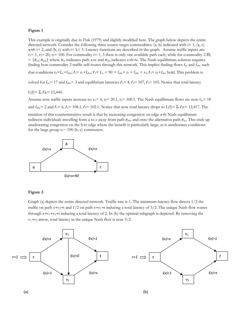
Figure 1
This example is originally due to Fisk (1979) and slightly modified here. The graph below depicts the entire directed network. Consider the following three source-target commodities: (a, b) indicated with i= 1, (a, c) with i= 2, and (b, c) with i= k= 3. Latency functions are described in the graph. Assume traffic inputs are: r1= 1, r2= 20, r3= 100. For commodity i= 1, 3 there is only one available path each, while for commodity 2 P2 = {pac; pabc} where pac indicates path azc and pabc indicates azbzc. The Nash equilibrium solution requires finding how commodity 2 traffic self-routes through this network. This implies finding flows fac and fabc such
that conditions r2=fac+fabc; {1= r1+fabc; {2= fac + 90 = fabc+ r1 + fabc + r3; {3= r3+fabc hold. This problem is
solved for fac= 17 and fabc= 3 and equilibrium latencies {1= 4, {2= 107, {3= 103. Notice that total latency
L(f)= Si {iri= 12,444.
Assume now traffic inputs increase to: r1= 4, r2= 20.1, r3= 100.1. The Nash equilibrium flows are now fac= 18
and fabc= 2 and {1= 6, {2= 108.1, {3= 102.1. Notice that now total latency drops to L(f)= Si {iri= 12,417. The
intuition of this counterintuitive result is that by increasing congestion on edge azb Nash equilibrium redirects individuals travelling form a to c away from path pabc and onto the alternative path pac. This ends up ameliorating congestion on the bzc edge where the benefit is particularly large, as it ameliorates conditions for the large group r3~ 100 (b, c) commuters.
Figure 2
Graph (a) depicts the entire directed network. Traffic rate is 1. The minimum-latency flow directs 1/2 the traffic on path szv2zt and 1/2 on path szv1zt inducing a total latency of 3/2. The unique Nash flow routes through szv1zv2zt inducing a total latency of 2. In (b) the optimal subgraph is depicted. By removing the v1zv2 arrow, total latency in the unique Nash flow is now 3/2.
l(x)=0
l(x)=1
l(x)=x
s
v2
v1
t
l(x)=1
l(x)=x
r=1
(a)
l(x)=1
l(x)=x
s
v2
v1
t
l(x)=1
l(x)=x
r=1
(b)
l(x)=x+90
l(x)=x
a
b
c
l(x)=x
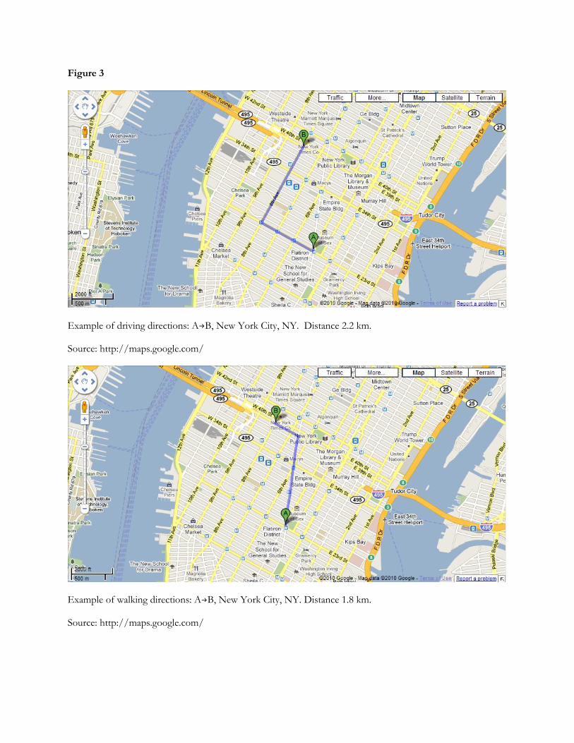
Figure 3
Example of driving directions: AzB, New York City, NY. Distance 2.2 km.
Source: http://maps.google.com/
Example of walking directions: AzB, New York City, NY. Distance 1.8 km.
Source: http://maps.google.com/
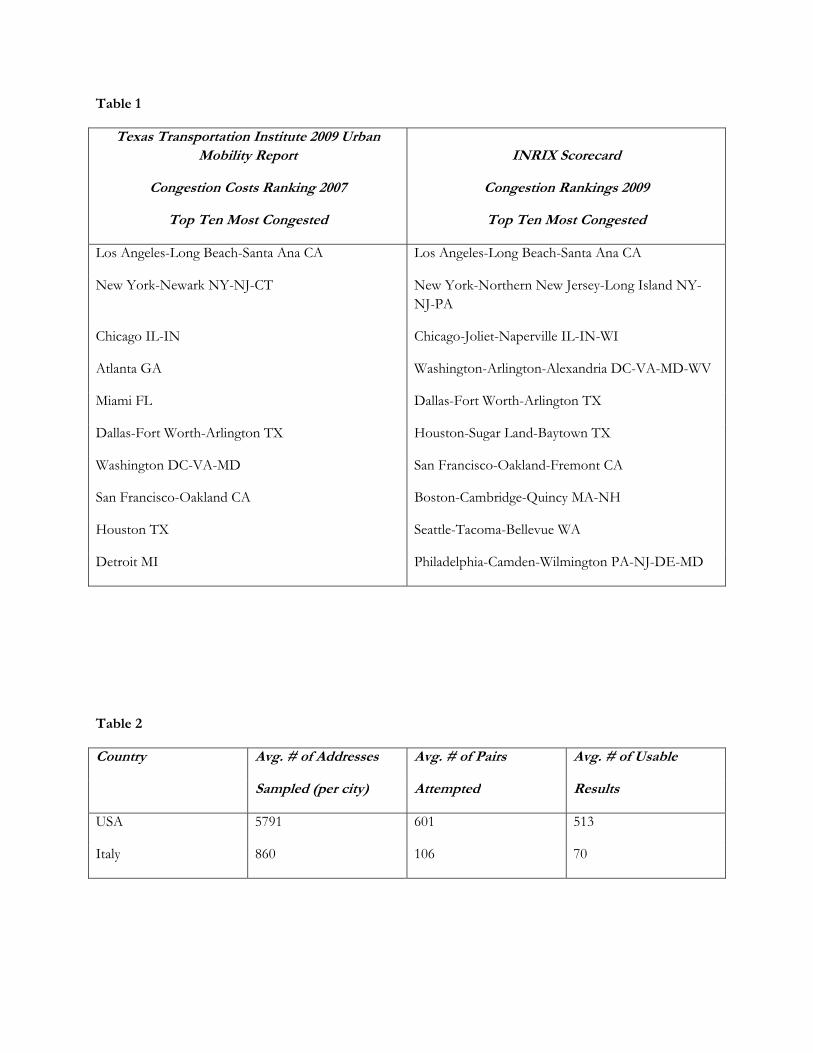
Table 1
Texas Transportation Institute 2009 Urban Mobility Report
Congestion Costs Ranking 2007
Top Ten Most Congested
INRIX Scorecard
Congestion Rankings 2009
Top Ten Most Congested
Los Angeles-Long Beach-Santa Ana CA Los Angeles-Long Beach-Santa Ana CA
New York-Newark NY-NJ-CT New York-Northern New Jersey-Long Island NY-NJ-PA
Chicago IL-IN Chicago-Joliet-Naperville IL-IN-WI
Atlanta GA Washington-Arlington-Alexandria DC-VA-MD-WV
Miami FL Dallas-Fort Worth-Arlington TX
Dallas-Fort Worth-Arlington TX Houston-Sugar Land-Baytown TX
Washington DC-VA-MD San Francisco-Oakland-Fremont CA
San Francisco-Oakland CA Boston-Cambridge-Quincy MA-NH
Houston TX Seattle-Tacoma-Bellevue WA
Detroit MI Philadelphia-Camden-Wilmington PA-NJ-DE-MD
Table 2
Country Avg. # of Addresses Avg. # of Pairs Avg. # of Usable
Sampled (per city) Attempted Results
USA 5791 601 513
Italy 860 106 70
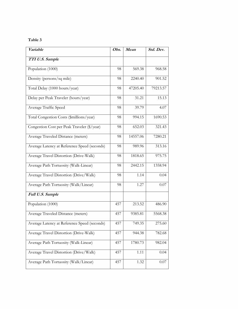
Table 3
Variable Obs. Mean Std. Dev.
TTI U.S. Sample
Population (1000) 98 569.38 968.58
Density (persons/sq mile) 98 2240.40 901.52
Total Delay (1000 hours/year) 98 47205.40 79213.57
Delay per Peak Traveler (hours/year) 98 31.21 15.13
Average Traffic Speed 98 39.79 4.07
Total Congestion Costs ($millions/year) 98 994.15 1690.53
Congestion Cost per Peak Traveler ($/year) 98 652.03 321.43
Average Traveled Distance (meters) 98 14557.06 7280.21
Average Latency at Reference Speed (seconds) 98 989.96 313.16
Average Travel Distortion (Drive-Walk) 98 1818.65 975.75
Average Path Tortuosity (Walk-Linear) 98 2442.15 1358.94
Average Travel Distortion (Drive/Walk) 98 1.14 0.04
Average Path Tortuosity (Walk/Linear) 98 1.27 0.07
Full U.S. Sample
Population (1000) 457 213.52 486.90
Average Traveled Distance (meters) 457 9385.81 5568.38
Average Latency at Reference Speed (seconds) 457 749.35 275.60
Average Travel Distortion (Drive-Walk) 457 944.38 782.68
Average Path Tortuosity (Walk-Linear) 457 1780.73 982.04
Average Travel Distortion (Drive/Walk) 457 1.11 0.04
Average Path Tortuosity (Walk/Linear) 457 1.32 0.07
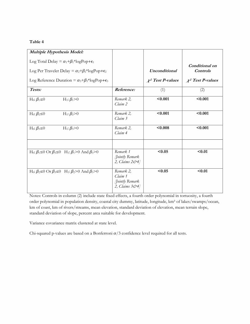
Table 4
Multiple Hypothesis Model:
Log Total Delay = a1+b1*logPop+e1
Log Per Traveler Delay = a2+b2*logPop+e2
Log Reference Duration = a3+b3*logPop+e3
Unconditional
c2 Test P-values
Conditional on Controls
c2 Test P-values
Tests: Reference: (1) (2)
H0: b1§0 H1: b1>0 Remark 2, Claim 2
<0.001 <0.001
H0: b2§0 H1: b2>0 Remark 2, Claim 3
<0.001 <0.001
H0: b3§0 H1: b3>0 Remark 2, Claim 4
<0.008 <0.001
H0: b1§0 Or b3§0 H1: b1>0 And b3>0 Remark 1 [Jointly Remark 2, Claims 2&4]
<0.05 <0.01
H0: b2§0 Or b3§0 H1: b2>0 And b3>0 Remark 2, Claim 1 [Jointly Remark 2, Claims 3&4]
<0.05 <0.01
Notes: Controls in column (2) include state fixed effects, a fourth order polynomial in tortuosity, a fourth order polynomial in population density, coastal city dummy, latitude, longitude, km² of lakes/swamps/ocean, km of coast, km of rivers/streams, mean elevation, standard deviation of elevation, mean terrain slope, standard deviation of slope, percent area suitable for development.
Variance covariance matrix clustered at state level.
Chi-squared p-values are based on a Bonferroni a/3 confidence level required for all tests.
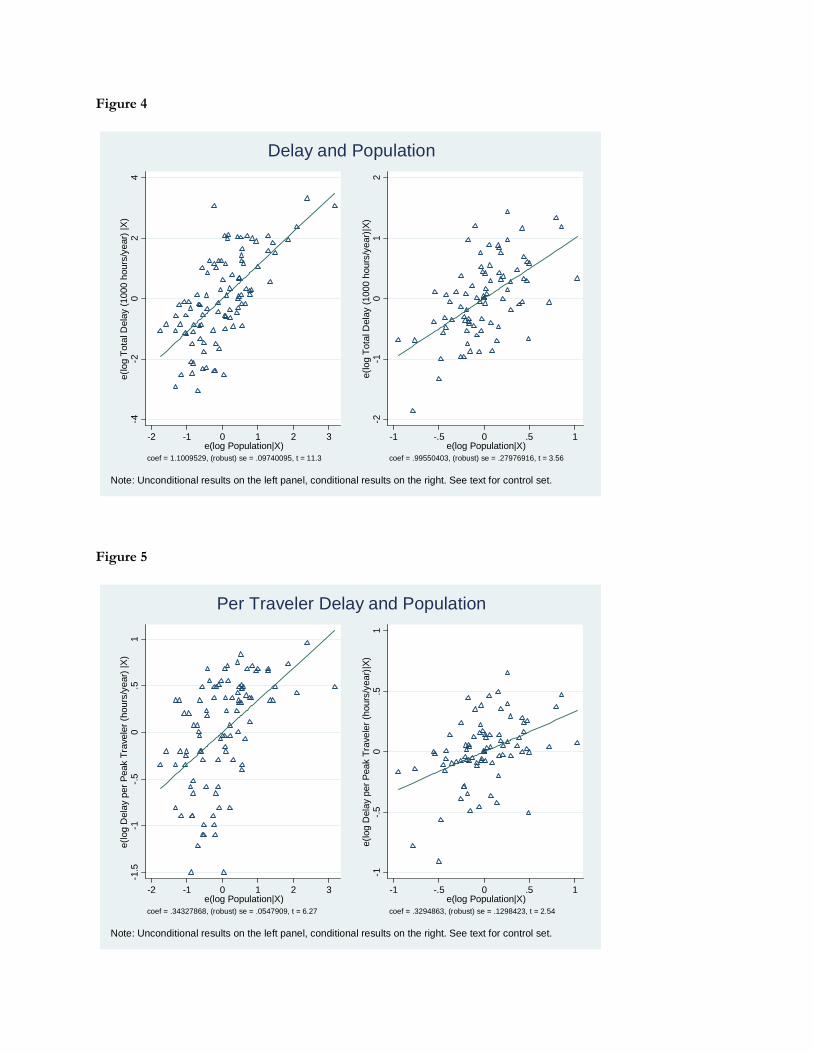
Figure 4
-4-2
02
4e(
log
Tot
al D
elay
(10
00 h
ours
/yea
r) |X
)
-2 -1 0 1 2 3e(log Population|X)
coef = 1.1009529, (robust) se = .09740095, t = 11.3
-2-1
01
2e(
log
Tot
al D
elay
(10
00 h
ours
/yea
r)|X
)
-1 -.5 0 .5 1e(log Population|X)
coef = .99550403, (robust) se = .27976916, t = 3.56
Note: Unconditional results on the left panel, conditional results on the right. See text for control set.
Delay and Population
Figure 5
-1.5
-1-.
50
.51
e(lo
g D
elay
per
Pea
k T
rave
ler
(hou
rs/y
ear)
|X)
-2 -1 0 1 2 3e(log Population|X)
coef = .34327868, (robust) se = .0547909, t = 6.27
-1-.
50
.51
e(lo
g D
elay
per
Pea
k T
rave
ler
(hou
rs/y
ear)
|X)
-1 -.5 0 .5 1e(log Population|X)
coef = .3294863, (robust) se = .1298423, t = 2.54
Note: Unconditional results on the left panel, conditional results on the right. See text for control set.
Per Traveler Delay and Population
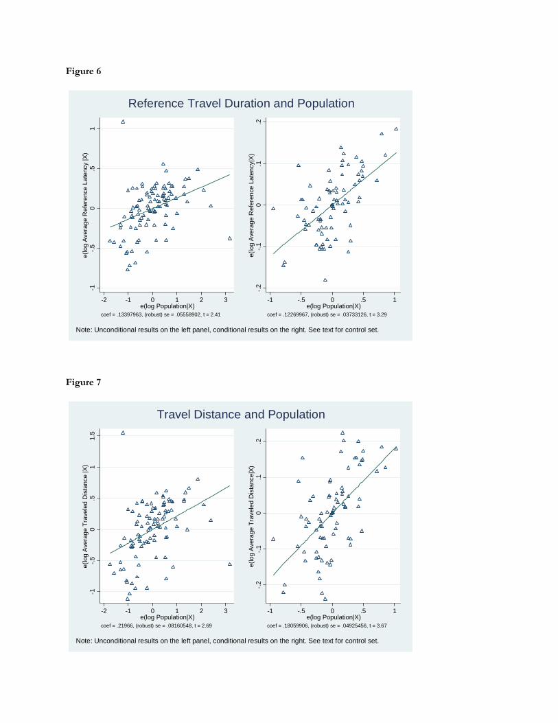
Figure 6
-1-.
50
.51
e(lo
g A
vera
ge R
efer
ence
Lat
ency
|X)
-2 -1 0 1 2 3e(log Population|X)
coef = .13397963, (robust) se = .05558902, t = 2.41
-.2
-.1
0.1
.2e(
log
Ave
rage
Ref
eren
ce L
aten
cy|X
)
-1 -.5 0 .5 1e(log Population|X)
coef = .12269967, (robust) se = .03733126, t = 3.29
Note: Unconditional results on the left panel, conditional results on the right. See text for control set.
Reference Travel Duration and Population
Figure 7
-1-.
50
.51
1.5
e(lo
g A
vera
ge T
rave
led
Dis
tanc
e |X
)
-2 -1 0 1 2 3e(log Population|X)
coef = .21966, (robust) se = .08160548, t = 2.69
-.2
-.1
0.1
.2e(
log
Ave
rage
Tra
vele
d D
ista
nce|
X)
-1 -.5 0 .5 1e(log Population|X)
coef = .18059906, (robust) se = .04925456, t = 3.67
Note: Unconditional results on the left panel, conditional results on the right. See text for control set.
Travel Distance and Population
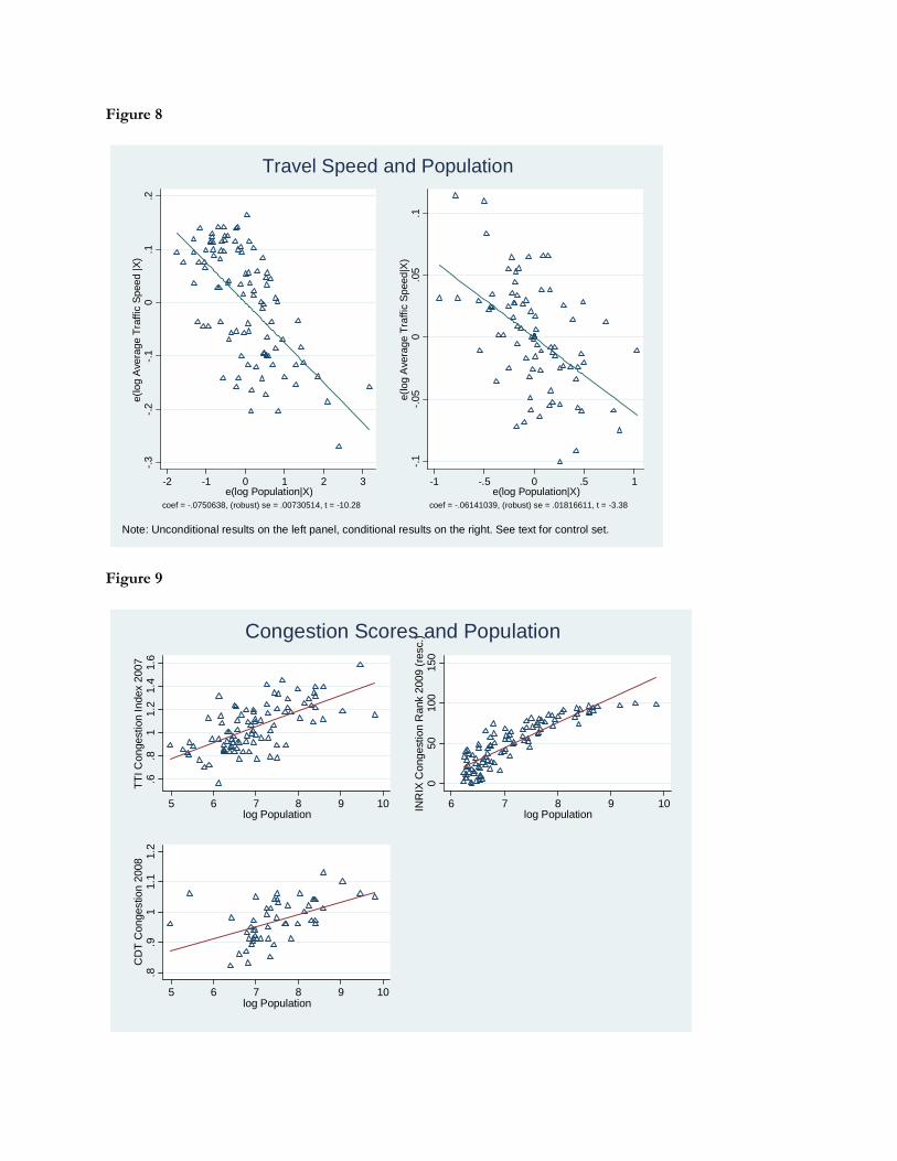
Figure 8
-.3
-.2
-.1
0.1
.2e(
log
Ave
rage
Tra
ffic
Spe
ed |X
)
-2 -1 0 1 2 3e(log Population|X)
coef = -.0750638, (robust) se = .00730514, t = -10.28
-.1
-.05
0.0
5.1
e(lo
g A
vera
ge T
raffi
c S
peed
|X)
-1 -.5 0 .5 1e(log Population|X)
coef = -.06141039, (robust) se = .01816611, t = -3.38
Note: Unconditional results on the left panel, conditional results on the right. See text for control set.
Travel Speed and Population
Figure 9
.6.8
11.
21.
41.
6T
TI C
onge
stio
n In
dex
2007
5 6 7 8 9 10log Population
050
100
150
INR
IX C
onge
stio
n R
ank
2009
(re
sc.)
6 7 8 9 10log Population
.8.9
11.
11.
2C
DT
Con
gest
ion
2008
5 6 7 8 9 10log Population
Congestion Scores and Population
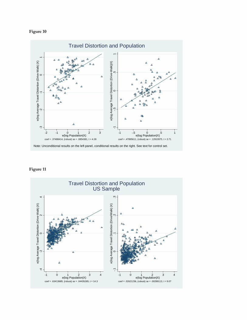
Figure 10
-3-2
-10
1e(
log
Ave
rage
Tra
vel D
isto
rtio
n (D
rive-
Wal
k) |X
)
-2 -1 0 1 2 3e(log Population|X)
coef = .37488414, (robust) se = .0854381, t = 4.39
-1-.
50
.51
e(lo
g A
vera
ge T
rave
l Dis
tort
ion
(Driv
e-W
alk)
|X)
-1 -.5 0 .5 1e(log Population|X)
coef = .47895611, (robust) se = .12910975, t = 3.71
Note: Unconditional results on the left panel, conditional results on the right. See text for control set.
Travel Distortion and Population
Figure 11
-4-2
02
4e(
log
Ave
rage
Tra
vel D
isto
rtio
n (D
rive-
Wal
k) |X
)
-1 0 1 2 3 4e(log Population|X)
coef = .63413685, (robust) se = .04435265, t = 14.3
-.1
0.1
.2.3
e(lo
g A
vera
ge T
rave
l Dis
tort
ion
(Driv
e/W
alk)
|X)
-1 0 1 2 3 4e(log Population|X)
coef = .02621236, (robust) se = .00289113, t = 9.07
Travel Distortion and PopulationUS Sample
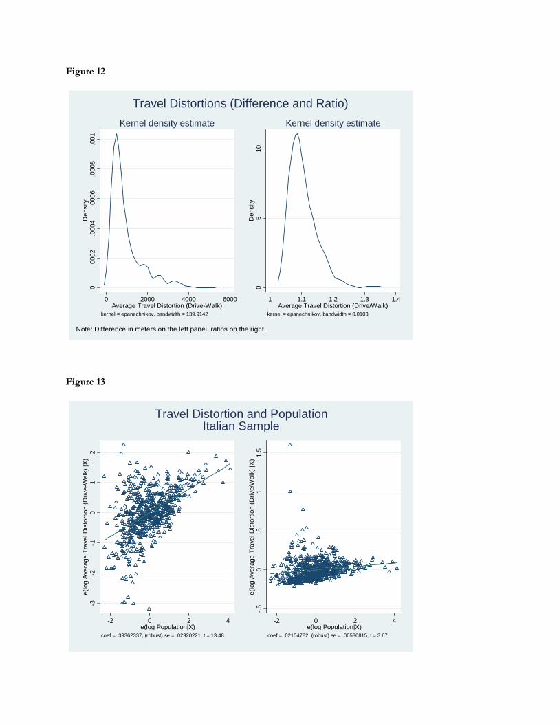
Figure 12
0.0
002
.000
4.0
006
.000
8.0
01D
ensi
ty
0 2000 4000 6000Average Travel Distortion (Drive-Walk)
kernel = epanechnikov, bandwidth = 139.9142
Kernel density estimate
05
10D
ensi
ty
1 1.1 1.2 1.3 1.4Average Travel Distortion (Drive/Walk)
kernel = epanechnikov, bandwidth = 0.0103
Kernel density estimate
Note: Difference in meters on the left panel, ratios on the right.
Travel Distortions (Difference and Ratio)
Figure 13
-3-2
-10
12
e(lo
g A
vera
ge T
rave
l Dis
tort
ion
(Driv
e-W
alk)
|X)
-2 0 2 4e(log Population|X)
coef = .39362337, (robust) se = .02920221, t = 13.48
-.5
0.5
11.
5e(
log
Ave
rage
Tra
vel D
isto
rtio
n (D
rive/
Wal
k) |X
)
-2 0 2 4e(log Population|X)
coef = .02154782, (robust) se = .00586815, t = 3.67
Travel Distortion and PopulationItalian Sample