galapagos islands. metapopulation models species area curves (islands as case study) review of...
TRANSCRIPT

Galapagos Islands
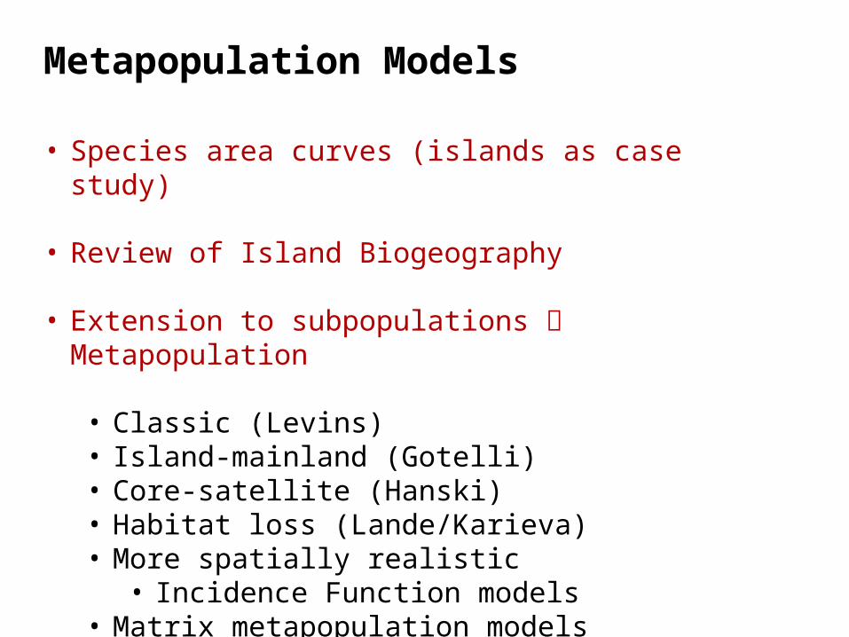
Metapopulation Models
• Species area curves (islands as case study)
• Review of Island Biogeography
• Extension to subpopulations Metapopulation
• Classic (Levins)• Island-mainland (Gotelli)• Core-satellite (Hanski)• Habitat loss (Lande/Karieva)• More spatially realistic
• Incidence Function models • Matrix metapopulation models
(Ozgul et al. 2008 Am. Nat.)
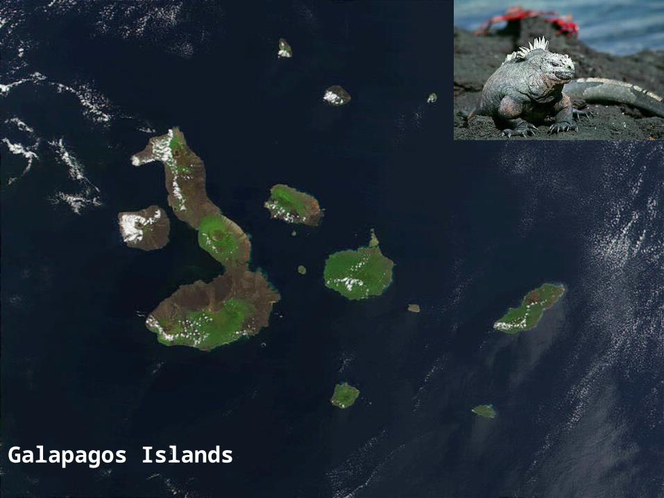
Galapagos Islands
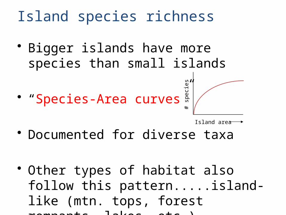
Island species richness
• Bigger islands have more species than small islands
• “Species-Area curves”
• Documented for diverse taxa
• Other types of habitat also follow this pattern.....island-like (mtn. tops, forest remnants, lakes, etc.)
Island area
# s
peci
es
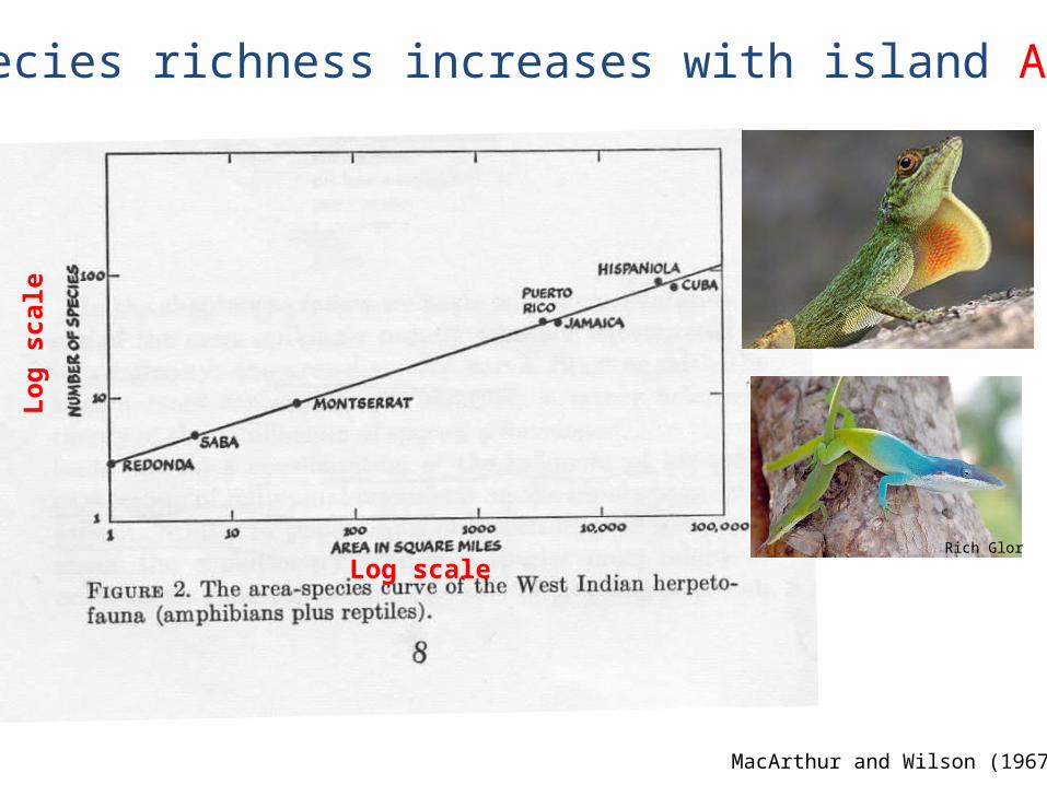
Species richness increases with island AREA
MacArthur and Wilson (1967)
Rich Glor
Lo
g s
cale
Log scale
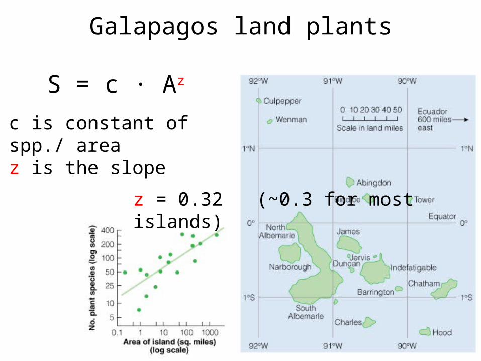
Galapagos land plants
S = c · Az
c is constant of spp./ areaz is the slope
z = 0.32 (~0.3 for most islands)
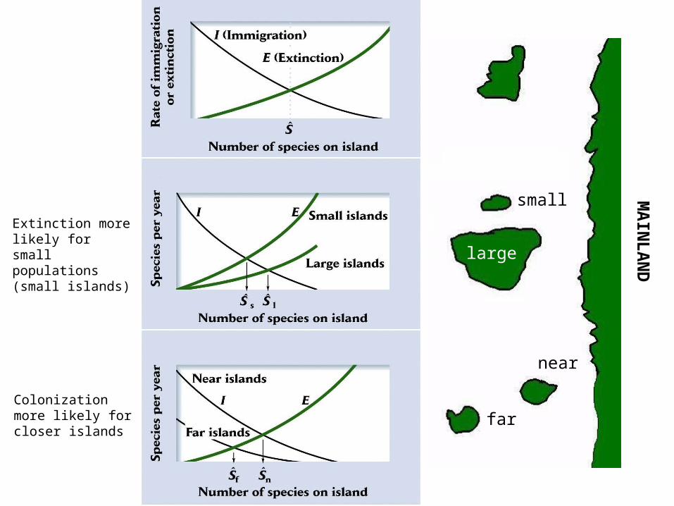
An extension of this idea:Island biogeography
• Dynamic equilibrium theory that explains species richness of islands
• Island richness determined by colonization and extinction rates (number of species thru time)
• Richness increases with size (more habiats to
support more species, less extinction).... decreases with isolation (less likely to be colonized)
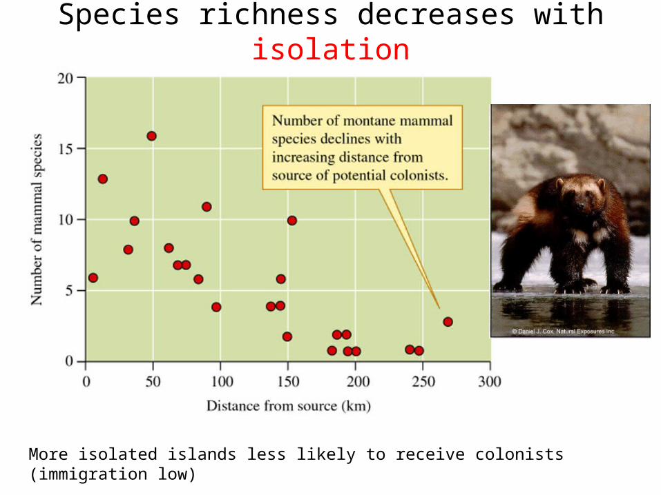
Species richness decreases with isolation
More isolated islands less likely to receive colonists (immigration low)
MA
INLA
ND
large
small
near
far
Extinction more likely for small populations (small islands)
Colonization more likely for closer islands
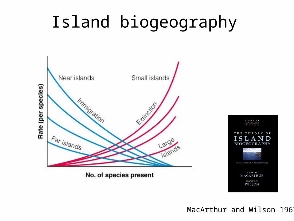
Island biogeography
MacArthur and Wilson 1967
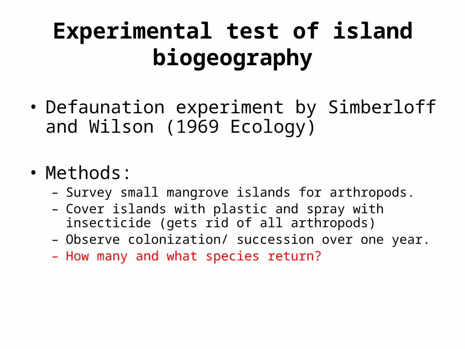
Experimental test of island biogeography
• Defaunation experiment by Simberloff and Wilson (1969 Ecology)
• Methods:– Survey small mangrove islands for arthropods.– Cover islands with plastic and spray with insecticide
(gets rid of all arthropods)– Observe colonization/ succession over one year. – How many and what species return?
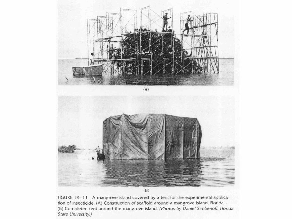
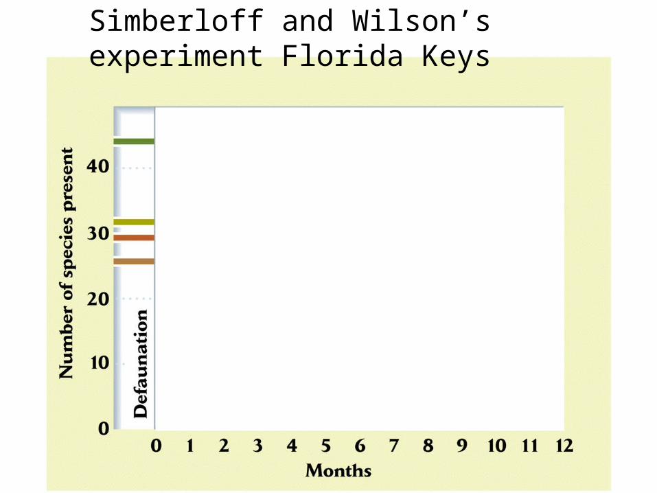
Simberloff and Wilson’s experiment Florida Keys
Results
• Species richness on islands returned to levels similar to before defaunation
• Closer, larger islands had more species
• The precise species identity was not consistent, only the total number of species – Order of colonization and species
interactions important for “who” composes the community
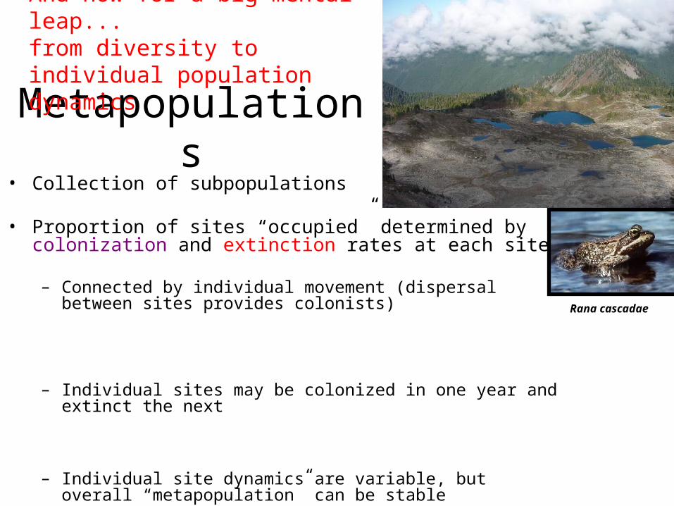
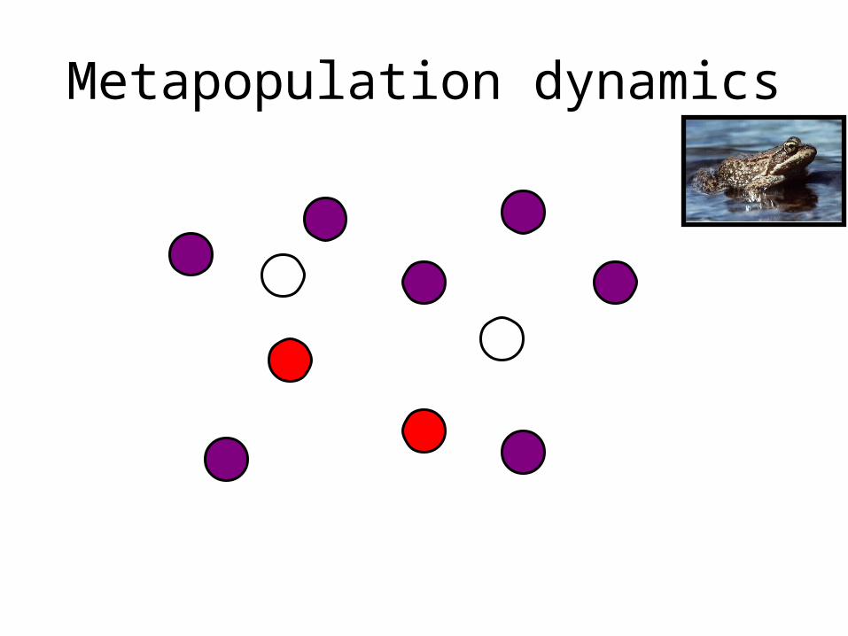
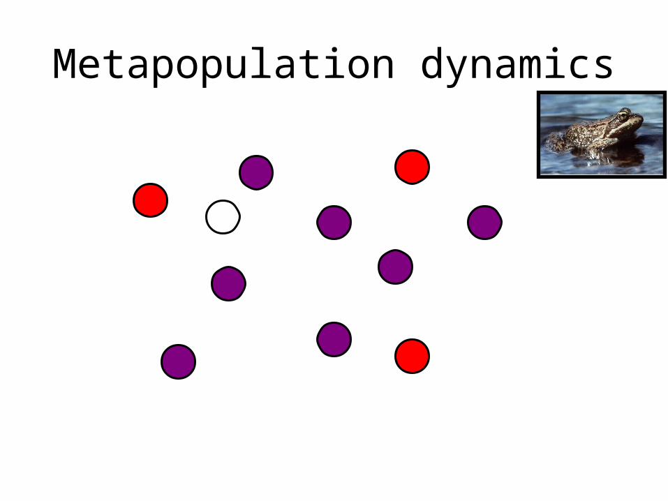
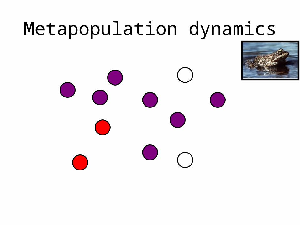
Metapopulations• Collection of subpopulations
• Proportion of sites “occupied” determined by colonization and extinction rates at each site
– Connected by individual movement (dispersal between sites provides colonists)
– Individual sites may be colonized in one year and extinct the next
– Individual site dynamics are variable, but overall “metapopulation” can be stable
And now for a big mental leap...from diversity to individual population dynamics
Rana cascadae
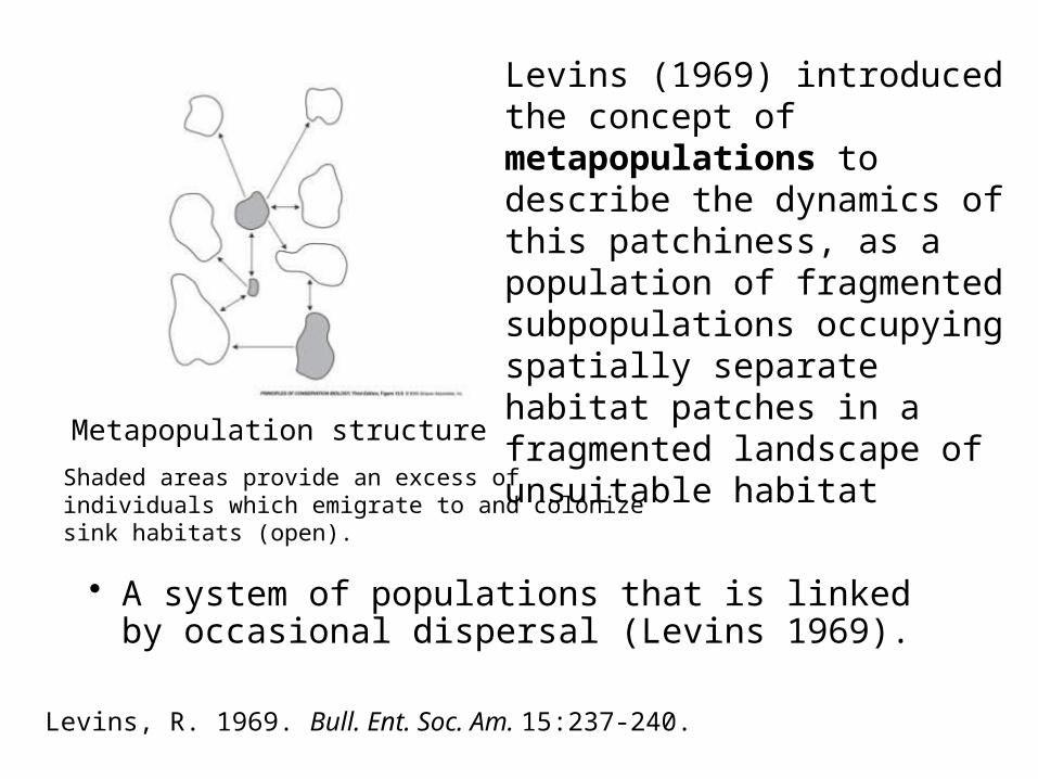
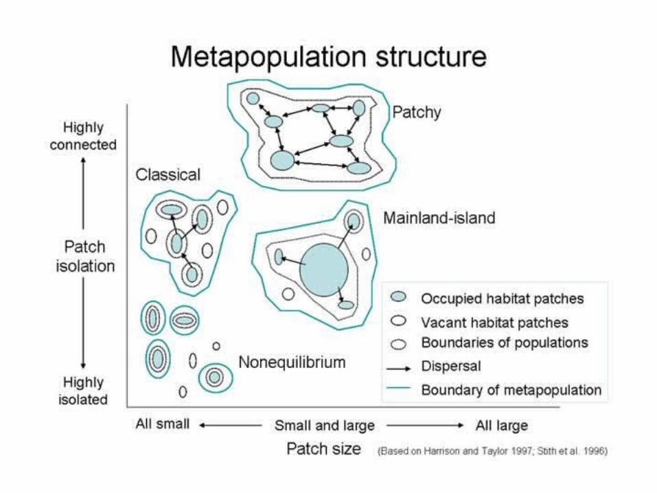
Metapopulation structure
Levins (1969) introduced the concept of metapopulations to describe the dynamics of this patchiness, as a population of fragmented subpopulations occupying spatially separate habitat patches in a fragmented landscape of unsuitable habitat
• A system of populations that is linked by occasional dispersal (Levins 1969).
Levins, R. 1969. Bull. Ent. Soc. Am. 15:237-240.
Shaded areas provide an excess of individuals which emigrate to and colonize sink habitats (open).
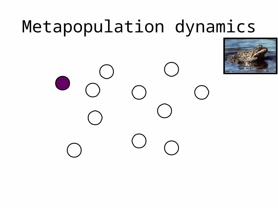
Metapopulation dynamics
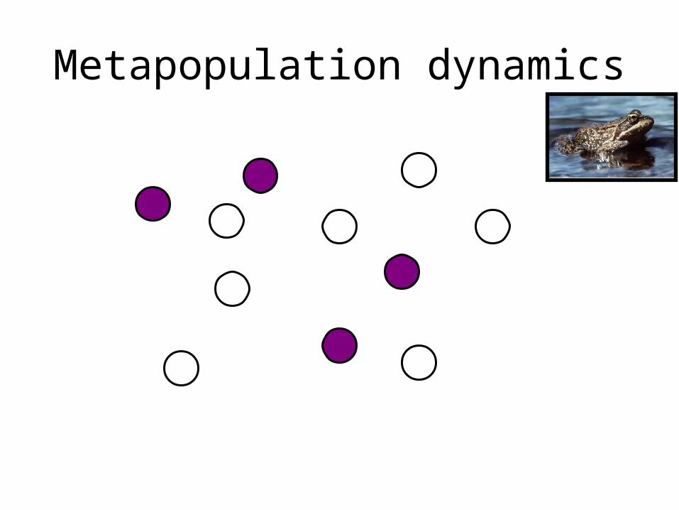
Metapopulation dynamics
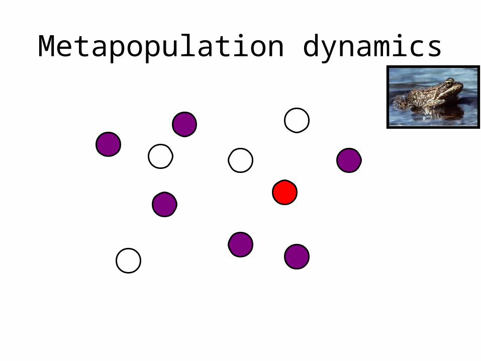
Metapopulation dynamics
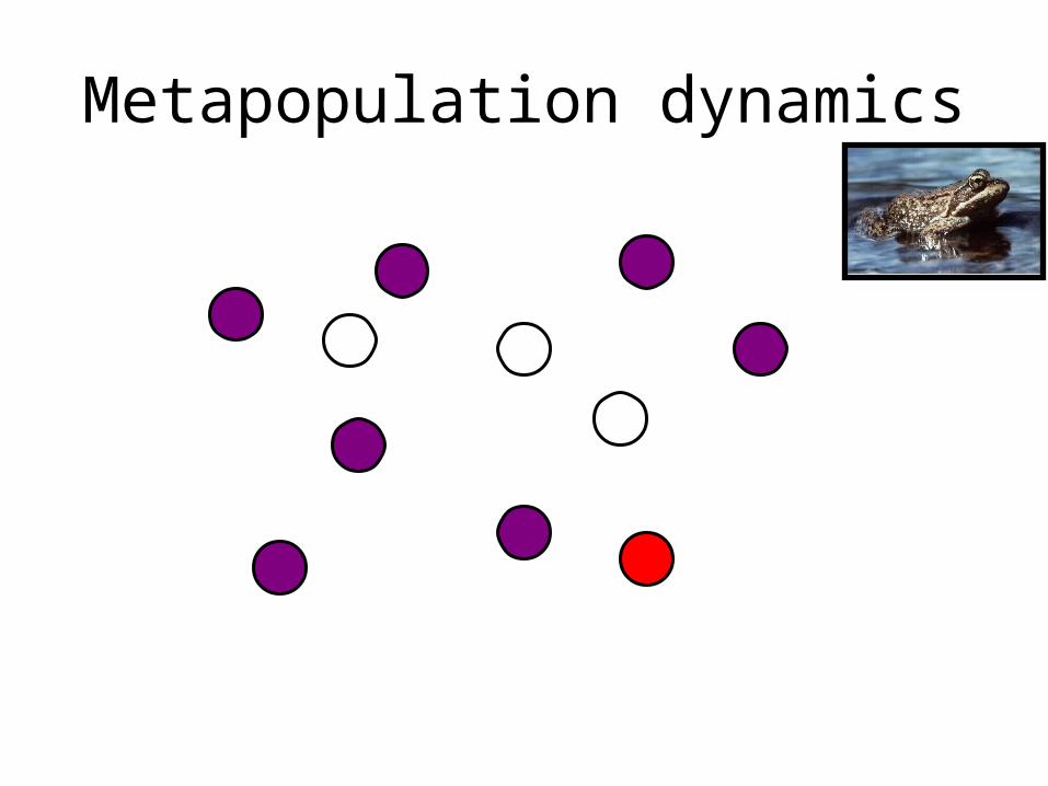
Metapopulation dynamics
Metapopulation dynamics
Metapopulation dynamics
Metapopulation dynamics
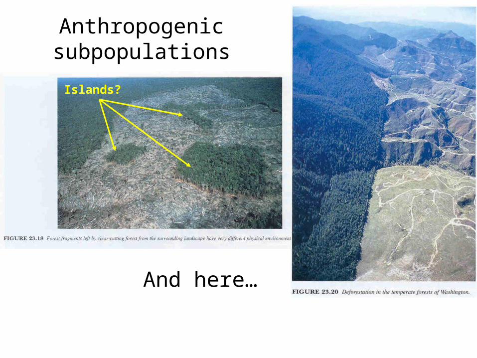
Anthropogenic subpopulations
And here…
Islands?
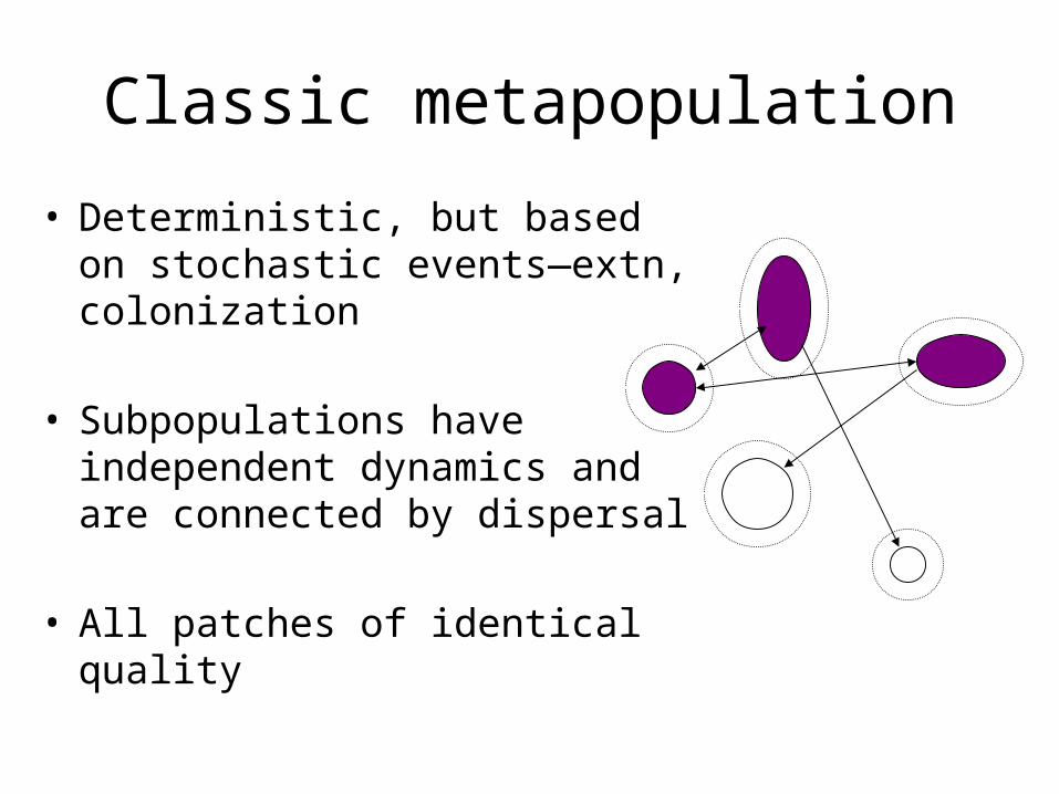
Classic metapopulation
• Deterministic, but based on stochastic events—extn, colonization
• Subpopulations have independent dynamics and are connected by dispersal
• All patches of identical quality
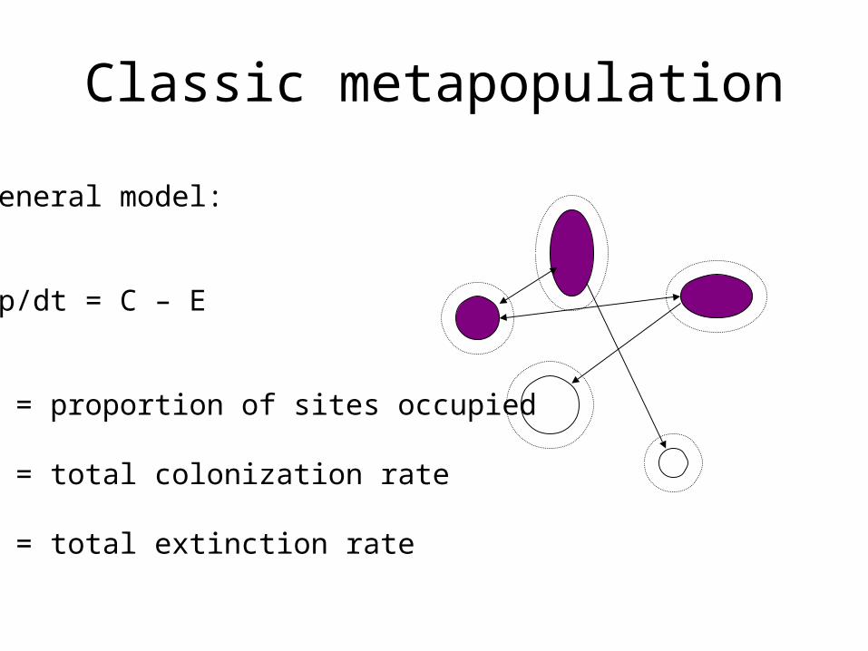
Classic metapopulation
General model:
dp/dt = C – E
p = proportion of sites occupied
C = total colonization rate
E = total extinction rate
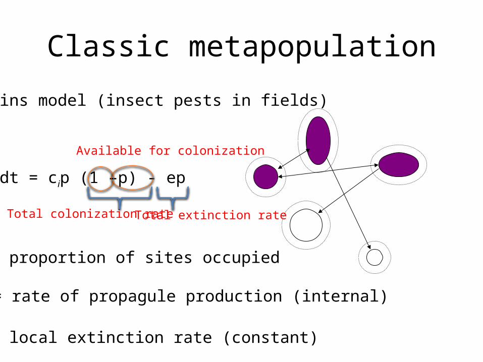
Classic metapopulation
Levins model (insect pests in fields)
dp/dt = cip (1 –p) - ep
p = proportion of sites occupied
ci = rate of propagule production (internal)
e = local extinction rate (constant)
Available for colonization
Total colonization rate Total extinction rate
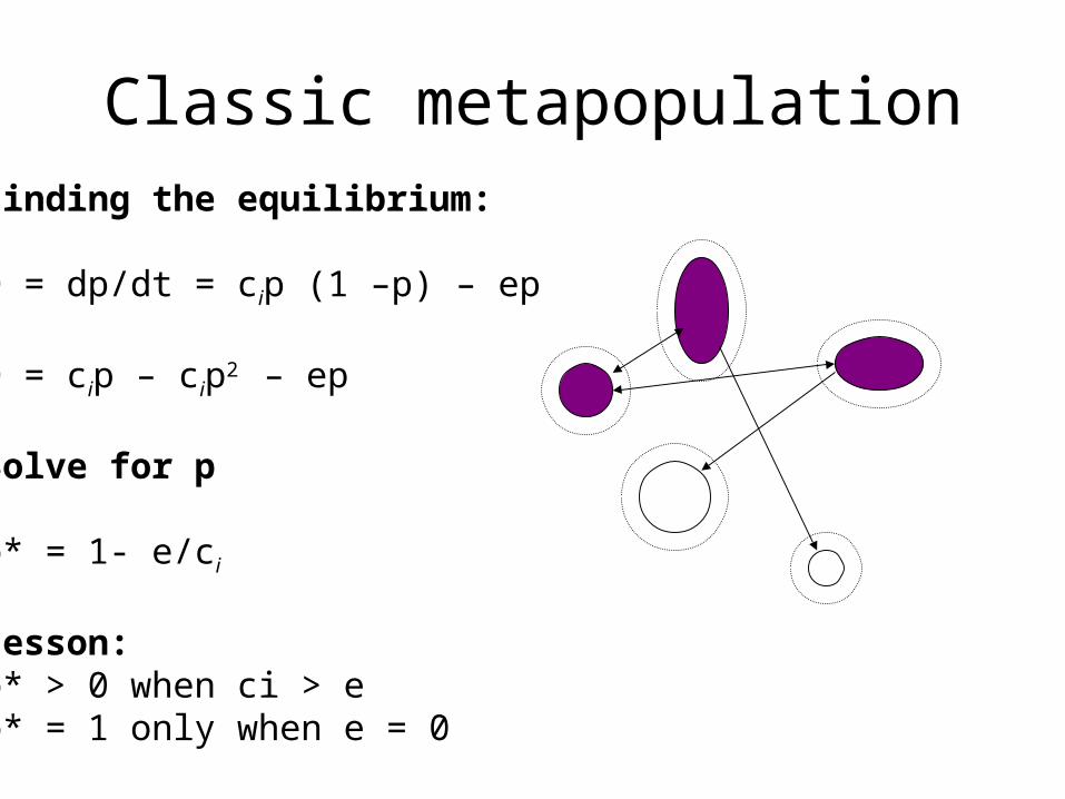
Classic metapopulationFinding the equilibrium:
0 = dp/dt = cip (1 –p) – ep
0 = cip – cip2 – ep
Solve for p
p* = 1- e/ci
Lesson: p* > 0 when ci > ep* = 1 only when e = 0
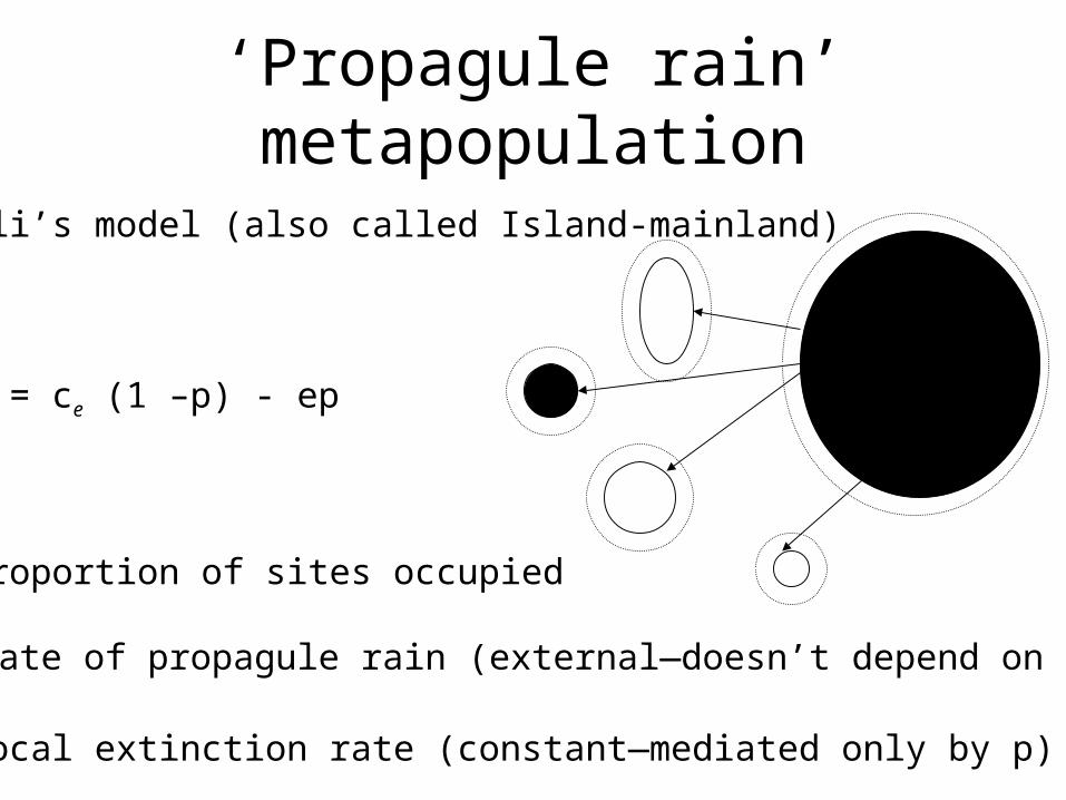
Gotelli’s model (also called Island-mainland)
dp/dt = ce (1 –p) - ep
p = proportion of sites occupied
ce = rate of propagule rain (external—doesn’t depend on p)
e = local extinction rate (constant—mediated only by p)
‘Propagule rain’ metapopulation

‘Propagule rain’ metapopulation
Finding the equilibrium:
0 = dp/dt = ce (1 –p) – ep
0 = ce – cep – ep
Solve for p
p* = ce /(ce + e)
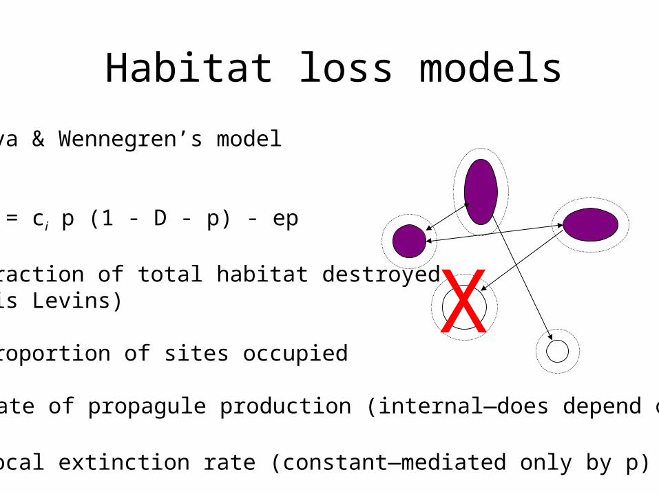
Habitat loss models
X
Karieva & Wennegren’s model
dp/dt = ci p (1 - D - p) - ep
D = fraction of total habitat destroyed(D=0 is Levins)
p = proportion of sites occupied
ci = rate of propagule production (internal—does depend on p)
e = local extinction rate (constant—mediated only by p)
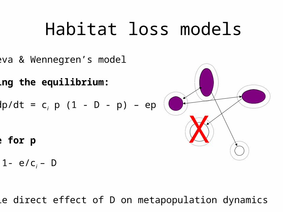
Habitat loss models
X
Karieva & Wennegren’s model
Finding the equilibrium:
0 = dp/dt = ci p (1 - D - p) – ep
Solve for p
p* = 1- e/ci – D
Simple direct effect of D on metapopulation dynamics
Assumptions of classic models:
• Identical patch ‘quality’ • Extinctions occur independently, local
dynamics are asynchronous • Colonization spreads across patch network
and all equally likely • All patches equally connected to all other
patches (not spatially explicit)• No population counts or size. Only suitable vs.
unsuitable, occupied or unoccupied
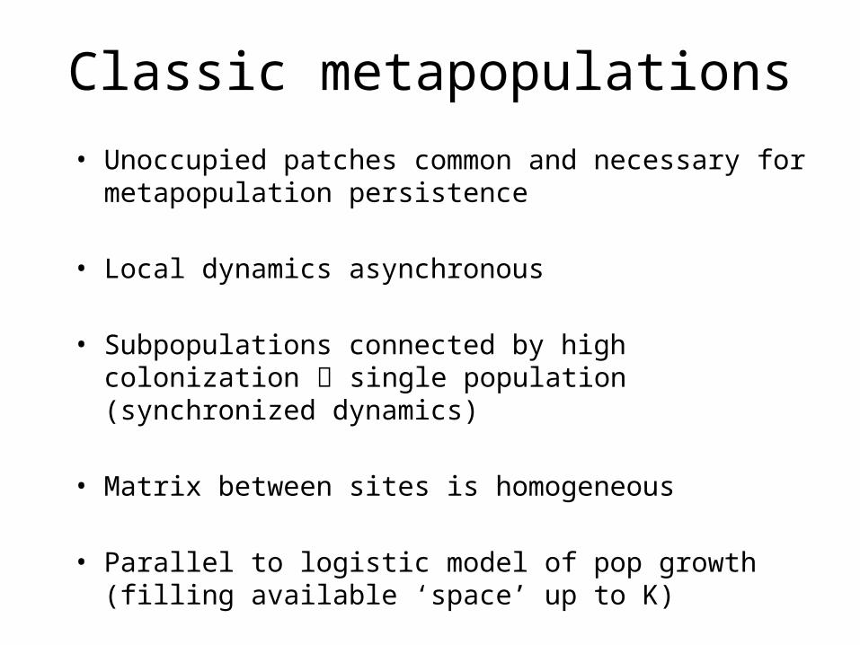
Classic metapopulations • Unoccupied patches common and
necessary for metapopulation persistence
• Local dynamics asynchronous
• Subpopulations connected by high colonization single population (synchronized dynamics)
• Matrix between sites is homogeneous
• Parallel to logistic model of pop growth (filling available ‘space’ up to K)
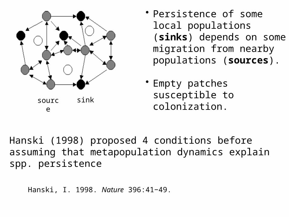
• Persistence of some local populations (sinks) depends on some migration from nearby populations (sources).
• Empty patches susceptible to colonization.
Hanski (1998) proposed 4 conditions before assuming that metapopulation dynamics explain spp. persistence
sinksource
Hanski, I. 1998. Nature 396:41−49.
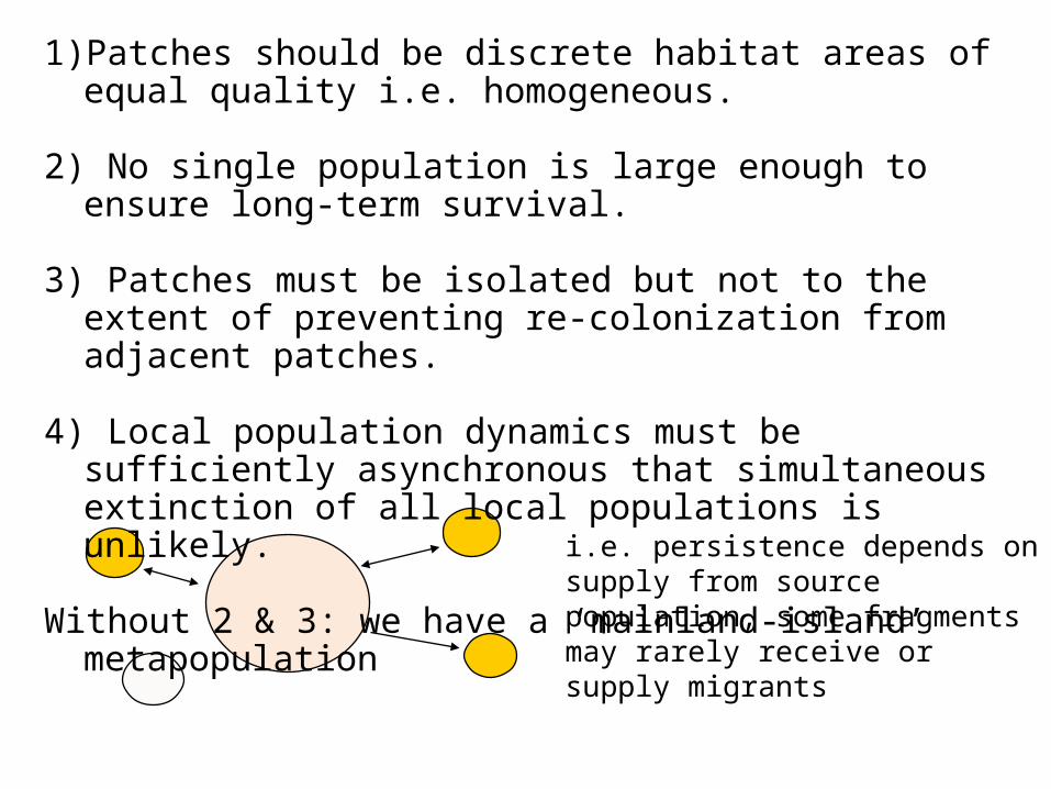
i.e. persistence depends on supply from source population, some fragments may rarely receive or supply migrants
1) Patches should be discrete habitat areas of equal quality i.e. homogeneous.
2) No single population is large enough to ensure long-term survival.
3) Patches must be isolated but not to the extent of preventing re-colonization from adjacent patches.
4) Local population dynamics must be sufficiently asynchronous that simultaneous extinction of all local populations is unlikely.
Without 2 & 3: we have a ‘mainland-island’ metapopulation
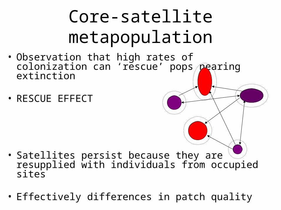
Core-satellite metapopulation
• Observation that high rates of colonization can ‘rescue’ pops nearing extinction
• RESCUE EFFECT
• Satellites persist because they are resupplied with individuals from occupied sites
• Effectively differences in patch quality
Core-satellite metapopulation
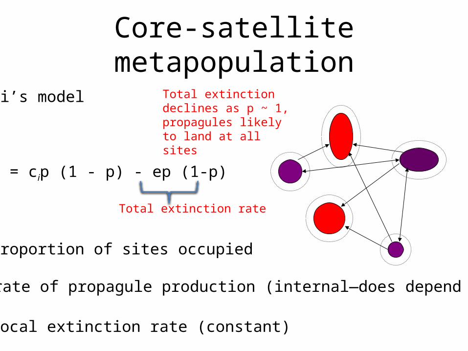
Hanski’s model
dp/dt = cip (1 - p) - ep (1-p)
p = proportion of sites occupied
ci = rate of propagule production (internal—does depend on p)
e = local extinction rate (constant)
Total extinction rate
Total extinction declines as p ~ 1, propagules likely to land at all sites
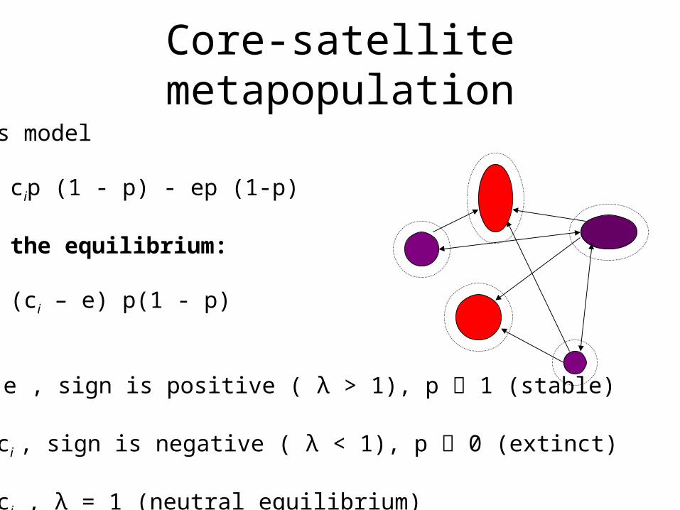
Core-satellite metapopulation
Hanski’s model
dp/dt = cip (1 - p) - ep (1-p)
Finding the equilibrium:
dp/dt = (ci – e) p(1 - p)
Notice: If ci > e , sign is positive ( λ > 1), p 1 (stable)
If e > ci , sign is negative ( λ < 1), p 0 (extinct)
If e = ci , λ = 1 (neutral equilibrium)
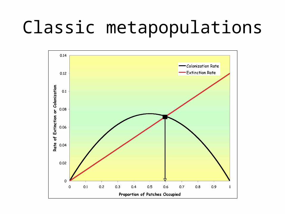
Classic metapopulations
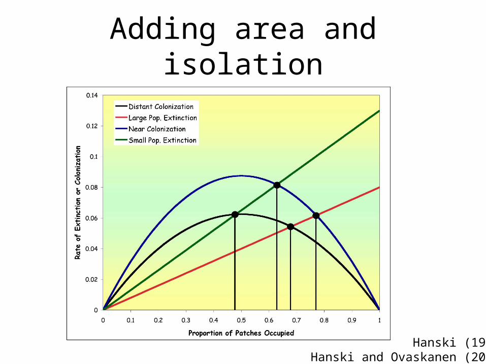
Adding area and isolation
Hanski (1991)Hanski and Ovaskanen (2003)
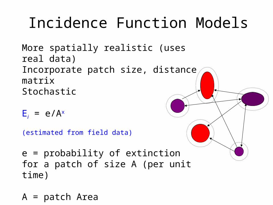
Incidence Function ModelsMore spatially realistic (uses real data)Incorporate patch size, distance matrixStochastic
Ei = e/Ax
(estimated from field data)
e = probability of extinction for a patch of size A (per unit time)
A = patch Area
x = demographic & environmental stochasticity (if large, E decreases fast with A)
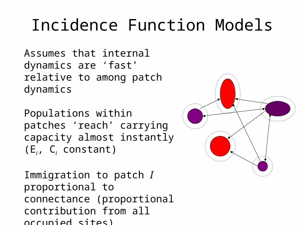
Incidence Function ModelsAssumes that internal dynamics are ‘fast’ relative to among patch dynamics
Populations within patches ‘reach’ carrying capacity almost instantly (Ei, Ci constant)
Immigration to patch I proportional to connectance (proportional contribution from all occupied sites)
Can evaluate the importance of patch loss on overall stability