gambling impact and behavior study · chapter 1. comparison between the results of the 1975 and...
TRANSCRIPT

*$0%/,1*�,03$&7�$1'�%(+$9,25�678'<
5HSRUW�WR�WKH1DWLRQDO�*DPEOLQJ�,PSDFW�6WXG\�&RPPLVVLRQ
$SULO��������
6XEPLWWHG�%\
'HDQ�*HUVWHLQ� 6DOO\�0XUSK\� 0DULDQQD�7RFH-RKQ�+RIIPDQQ� $PDQGD�3DOPHU� 5REHUW�-RKQVRQ&LQG\�/DULVRQ /XFLDQ�&KXFKUR 7UDF\�%XLH/DV]OR�(QJHOPDQ 0DU\�$QQ�+LOO
1DWLRQDO�2SLQLRQ�5HVHDUFK�&HQWHU�DW�WKH�8QLYHUVLW\�RI�&KLFDJRhttp://www.norc.uchicago.edu
5DFKHO�9ROEHUJ
*HPLQL�5HVHDUFK1RUWKDPSWRQ��0DVVDFKXVHWWV
http://www.geminiresearch.com
+HQULFN�+DUZRRG��$GDP�7XFNHU
7KH�/HZLQ�*URXS)DLUID[��9LUJLQLD
http://www.lewin.com
(XJHQH�&KULVWLDQVHQ��:LOO�&XPPLQJV���6HEDVWLDQ�6LQFODLU
&KULVWLDQVHQ�&XPPLQJV�$VVRFLDWHV1HZ�<RUN��1HZ�<RUN

*DPEOLQJ�,PSDFW�DQG�%HKDYLRU�6WXG\ �3DJH�L
7$%/(�2)�&217(176
LIST OF EXHIBITS ..................................................................................................................... iii
TABLES........................................................................................................................................ iiiFIGURES ...................................................................................................................................... iv
ACKNOWLEDGMENTS.............................................................................................................. vPRINCIPAL STAFF ......................................................................................................................... vNORC COLLABORATORS............................................................................................................. vOTHER CONTRIBUTORS ............................................................................................................... vi
HIGHLIGHTS.............................................................................................................................viiiBASIS OF FINDINGS....................................................................................................................viiiCHANGES IN GAMBLING PARTICIPATION OVER TIME................................................................viiiPATHOLOGICAL AND PROBLEM GAMBLING...............................................................................viiiYOUTH GAMBLING...................................................................................................................... ixCOMMUNITY IMPACT OF CASINOS................................................................................................ x
INTRODUCTION .......................................................................................................................... 1
CHAPTER 1. COMPARISON BETWEEN THE RESULTS OF THE 1975 AND 1998NATIONAL SURVEYS OF ADULT GAMBLING BEHAVIOR ............................................. 3
METHODS ..................................................................................................................................... 4OVERALL PREVALENCE RATES .................................................................................................... 6DEMOGRAPHICS OF GAMBLERS.................................................................................................... 6REFERENCES............................................................................................................................... 11
CHAPTER 2. THE PREVALENCE AND CORRELATES OF GAMBLING PROBLEMSAMONG ADULTS ....................................................................................................................... 12
THE SOCIAL CONSTRUCTION OF PSYCHIATRIC TOOLS ............................................................... 12MEASURING GAMBLING PROBLEMS........................................................................................... 13
Adopting the South Oaks Gambling Screen in population research..................................... 13Validating the South Oaks Gambling Screen........................................................................ 14The eclipse of the South Oaks Gambling Screen .................................................................. 14Emergence of a new standard: The DSM–IV....................................................................... 15
DEVELOPMENT OF THE NORC DSM–IV SCREEN FOR GAMBLING PROBLEMS (“THE NODS”).. 17Validity and reliability of the NODS..................................................................................... 20The NODS typology .............................................................................................................. 20The role of timeframe............................................................................................................ 21
PATRON SURVEY ........................................................................................................................ 22PREVALENCE RATES................................................................................................................... 25REGIONAL DIFFERENCES AND AVAILABILITY ............................................................................ 28ATTITUDES TOWARD GAMBLING ............................................................................................... 29CORRELATION WITH OTHER DISORDERS .................................................................................... 29GAMBLING EXPENDITURES ........................................................................................................ 31ASSESSING PROBLEM AND PATHOLOGICAL GAMBLING IN THE FUTURE..................................... 34REFERENCES...............................................................................................................................35

*DPEOLQJ�,PSDFW�DQG�%HKDYLRU�6WXG\ �3DJH�LL
CHAPTER 3. ECONOMIC ANALYSIS OF THE CONSEQUENCES OF GAMBLINGPROBLEMS AMONG ADULTS................................................................................................ 38
PRIOR STUDIES ON THE COSTS OF GAMBLING ............................................................................ 41COSTLY CONSEQUENCES OF GAMBLING .................................................................................... 41
Employment-related impacts ................................................................................................ 43Bankruptcy, debt, unemployment insurance and welfare...................................................... 45Criminal justice costs............................................................................................................ 47Divorce ................................................................................................................................. 48Health care ........................................................................................................................... 50Mental health care ................................................................................................................ 51Treatment for pathological gambling ................................................................................... 51Total costs of pathological gambling.................................................................................... 52
SUMMARY .................................................................................................................................. 53ANNEX 1: DESCRIPTION OF OUTCOME VARIABLES ................................................................... 55ANNEX 2: DESCRIPTION OF EXPLANATORY/INDEPENDENT VARIABLES .................................... 56ANNEX 3: METHODOLOGICAL NOTES FOR COSTS ..................................................................... 57REFERENCES............................................................................................................................... 58
CHAPTER 4. GAMBLING AMONG 16- AND 17-YEAR-OLD YOUTHS .......................... 61
CHAPTER 5. IMPACTS OF CASINO PROXIMITY ON SOCIAL AND ECONOMICOUTCOMES, 1980–1997: A MULTILEVEL TIME-SERIES ANALYSIS ........................... 65
DATA.......................................................................................................................................... 66METHODS ................................................................................................................................... 67RESULTS..................................................................................................................................... 70REFERENCES............................................................................................................................... 72
CHAPTER 6. CASE STUDIES OF THE EFFECT ON COMMUNITIES OF INCREASINGACCESS TO MAJOR GAMBLING FACILITIES .................................................................. 73
THE COMMUNITIES..................................................................................................................... 74Types of gaming .................................................................................................................... 74Economic outcomes .............................................................................................................. 76Other social benefits and costs ............................................................................................. 78Problem gambling................................................................................................................. 78Public opinion regarding gambling...................................................................................... 79
CASE STUDY ONE: FLORISSANT................................................................................................ 79Our respondents.................................................................................................................... 80Gaming in Florissant ............................................................................................................ 80Community changes.............................................................................................................. 80Current community issues..................................................................................................... 82Public views on gaming ........................................................................................................ 83
CASE STUDY TWO: HANSEN...................................................................................................... 84Our respondents.................................................................................................................... 84Gaming in Hansen ................................................................................................................ 84Community changes.............................................................................................................. 85Current community issues..................................................................................................... 88Public views on gaming ........................................................................................................ 88
REFERENCES............................................................................................................................... 89

*DPEOLQJ�,PSDFW�DQG�%HKDYLRU�6WXG\ �3DJH�LLL
/,67�2)�(;+,%,76
7DEOHV
Table 1. DSM–IV Criteria for Pathological Gambling ....................................................16
Table 2. DSM–IV Criteria and Matched NODS Lifetime Questions ..............................18
Table 3. Criteria for Classifying Respondents .................................................................21
Table 4. Patron Interviews ...............................................................................................23
Table 5. Key Characteristics in RDD, Patron, and Merged Adult Surveys .....................24
Table 6. Percentage Gambling Types Based on Lifetime and Past-Year NODSScores.................................................................................................................25
Table 7. Lifetime and Past-Year Prevalence of Gambling Problems AmongDemographic Groups, in Percentages................................................................26
Table 8. Attitudes Toward Gambling in RDD+Patron Survey, by Lifetime andPast-Year Gambler Type....................................................................................29
Table 9. Percentage of Lifetime and Past-Year Gambler Types by Health,Mental Health, Substance Abuse, and Other Problems .....................................30
Table 10. Estimated Annual Amount Ahead, Behind, or Spent (in Millions of Dollars)in the Past Year, 1998 (from RDD Data).........................................................32
Table 11. Employment Experiences, by Type of Gambler (Lifetime Only)....................44
Table 12. Annual Financial and Job Losses by Problem and Pathological Gamblers .....45
Table 13. Financial Characteristics and Impacts, by Type of Gambler ...........................46
Table 14. Financial Losses, by Type of Gambler.............................................................46
Table 15. Weighted Occurrence of Criminal Justice Consequences, byType of Gambler..............................................................................................48
Table 16. Criminal Justice Losses , by Type of Gambler ................................................48
Table 17. Marital and Health Status, by Type of Gambler ..............................................49
Table 18. Divorce and Health Costs, by Type of Gambler ..............................................51
Table 19. Selected Economic Costs of Pathological and Problem Gambling: Costs perPathological and Problem Gambler .................................................................52
Table 20. Economic Impacts of Major Health Problems .................................................53
Table 21. Summary of Comparisons Between Pathological, Problem, and Low-RiskGamblers..........................................................................................................58
Table 22. Casino Proximity Effects in Model 3...............................................................71
Table 23. Model 3 Parameter Estimates: Selected Outcome Measures ..........................72

*DPEOLQJ�,PSDFW�DQG�%HKDYLRU�6WXG\ �3DJH�LY
)LJXUHV
Figure 1. Past-Year and Lifetime Gaming, 1975 and 1998................................................7
Figure 1a. Past-Year Gambling by Selected Games, 1975 and 1998..................................7
Figure 2. Sex of Past-Year Gamblers, 1975 and 1998 .......................................................7
Figure 3. Lifetime Gaming by Sex, 1975 and 1998 ...........................................................8
Figure 4. Past-Year Gaming by Sex, 1975 and 1998 .........................................................8
Figure 5. Lifetime Gaming by Age Group, 1975 and 1998 ...............................................9
Figure 6. Past-Year Gaming by Age Group, 1975 and 1998 .............................................9
Figure 7. Age Distribution of Past-Year Gamblers Versus Age Distributionof the Adult Population, 1975 and 1998 ..........................................................10
Figure 8. Past-Year Bingo by Age Group, 1975 and 1998 ..............................................11
Figure 9. Past-Year Gambling Participation by Type of Game .......................................62

*DPEOLQJ�,PSDFW�DQG�%HKDYLRU�6WXG\���$FNQRZOHGJPHQWV 3DJH�Y
$&.12:/('*0(176
3ULQFLSDO�6WDII
Dean Gerstein, NORC’s senior research vice president, held lead scientific responsibilityfor the design, integrity, and analysis of the Gambling Impact & Behavior Study (GIBS).In addition, he wrote parts of this report, including the Highlights and Introduction, andcoauthored Chapters 1, 2, and 4. Dr. Gerstein studied at Reed College and HarvardUniversity. Sally Murphy, senior study director in NORC’s survey operations center andgraduate of the University of Denver, was the GIBS project director, responsible foroverall resource management and the implementation and procedures of data collection.Marianna Toce, research analyst, led the community case study task, served ascoordinator for development of the questionnaires, and was editor-in-chief of GIBSreports; she authored Chapters 1 and 6. She is a graduate of Mount Holyoke College.
John Hoffmann, senior research scientist, served as task leader for statistical analysis ofRDD and patron survey data and completion of the community database. Dr Hoffmannhas studied at James Madison University, Emory University, and the State University ofNew York at Albany. Amanda Palmer, survey specialist and graduate of the Universityof Chicago, served as GIBS assistant project director, preparing, managing, and assuringthe quality of day-to-day flows of study materials and information. Robert Johnson,senior survey methodologist, served as statistical analyst for the community database anddesigned and performed the merging of the RDD and patron samples; he authoredChapter 5. Dr. Johnson is a graduate of Oberlin College and the University of Michigan.
Cindy Larison, research analyst and alumna of Old Dominion University and theUniversity of Maryland, designed and implemented a large proportion of statisticalprogramming for the patron, youth, and combined adult datasets. Lucian Chuchro, whostudied at the University of Chicago, was manager of the adult and youth telephonesurvey operations, including the pilot, validity, and reliability studies. Tracy Buie is agraduate of the University of Dallas. She was overall supervisor of GIBS field operationsfor the patron survey, including recruitment, training, and development of procedures.Mary Ann Hill, senior survey methodologist, studied at Pomona College and UCLA; shewas sampling director for the RDD adult and youth surveys. Laszlo Engelmann, seniorstatistician, developed the community database sample and conducted initial harvestingof variables; he studied at Kalamazoo College and the University of Southern California.
125&�&ROODERUDWRUV
Rachel Volberg, president of Gemini Research, Ltd., contributed as senior investigator toall aspects of study design, implementation and analysis. In addition, Dr. Volbergcoauthored Chapters 2 and 4. She is a graduate of the University of California, SanDiego, and University of California, San Francisco. Henrick Harwood, vice president ofThe Lewin Group, served as task leader for economic analysis; he studied at StetsonUniversity and the University of North Carolina, Chapel Hill. Adam Tucker, researchassociate at The Lewin Group, contributed extensively to the statistical programming ofthe economic analysis; he is a graduate of Kenyon College. Messrs. Harwood andTucker authored Chapter 3. Eugene Christiansen, president of Christiansen/Cummings

*DPEOLQJ�,PSDFW�DQG�%HKDYLRU�6WXG\���$FNQRZOHGJPHQWV 3DJH�YL
Associates (CCA), graduated from the University of California, Berkeley; throughout thestudy he provided advice and information pertaining to community and economic aspectsof gambling. William Cummings, general manager of CCA, contributed to thecommunity database sample design and developed the estimates of community gamblingexpenditures; he studied at the Massachusetts Institute of Technology. SebastianSinclair, an associate of CCA, studied at New York University. He assisted indeveloping the estimates of community gambling expenditures.
2WKHU�&RQWULEXWRUV
The authors wish to acknowledge the important role played by an additional cadre ofNORC staff, whose dedication was essential to completion of the work. These staffmembers were Ann Anderson, Joyce Ashaye, Albert Bard, Haider Baig, Martin Barron,Maureen Bonner, Bradley Bouten, Angeline Bregianes, Angela Brittingham, SharonBrown, Dennis Bryson, Jody Dougherty, Nancy Farinella, Lynn Gallagher, Adrian Gil,Cheryl Gilbert, Gerry Griffin, Angela Hermann, Rita Jena, Ben King, Cynthia Knight,Heather Kwasigroch, Kathryn Malloy, Michael McNicholas, Bronwyn Nichols, MichaelO’Connell, Albert Pach, Imelda Perez, Ann Ragin, Kenneth Rasinski, Michael Rhea,Lenora Rodriguez, Annemarie Rosenlund, Alan Sanderson, Sam Schildhaus, JoannaSmall, Patrick Smillie, Howard Speizer, Janel Temple, Faiz Uddin, Cynthia Veldman,Karen Veldman, Woodly Westbrook, and Kirk Wolter.
We also benefited greatly from the work of a technical advisory committee composed ofDrs. Henry Lesieur at the Institute for Problem Gambling, Peter Reuter at the Universityof Maryland, and William Thompson at the University of Nevada, Las Vegas. Otheradvice and information of substantial help us came from James Breiling of the NationalInstitute of Mental Health, James Colliver at the National Institute on Drug Abuse, DavidFischer of the Department of the Treasury, Curtis Barrett at the University of Louisville,Philip Cook at Duke University, Sue Fisher at the University of Plymouth, DianeO’Rourke at the University of Illinois, I. Nelson Rose at Whittier Law School, RichardRosenthal at the University of California Los Angeles, Howard Shaffer at HarvardMedical School, and Randy Stinchfield at the University of Minnesota.
We appreciate the opportunity afforded us to work with the Commission staff, especiallyits executive director, Timothy Kelly, and research director, Doug Seay. We are greatlyin the debt of Research Subcommittee chair Leo McCarthy, for sustaining us throughseveral long seasons, and to Research Subcommittee members John Wilhelm and JamesDobson, and their respective assistants, Eric Altman and Ron Reno, for ideas andcritiques that were invariably thought-provoking and useful. We thank the Commissionchair, Kay Coles James, and all other members of the Commission for their support,encouragement, and constructive criticism.
We must note without specific attribution the cooperation given to our pilot and mainpatron surveys by members of the commercial gaming industry, ranging from multi-billion-dollar corporations to mom-and-pop stores, and the assistance to the validationstudy of the GIBS questionnaire given by a number of gambling treatment providers. Itis not a light matter to admit survey researchers onto the premises and among thecustomers or clients who provide one’s livelihood, and we are indebted to all of theindividual owners and corporate officers who were gracious enough to do so. We werealso beneficiaries of the good offices of the American Gaming Association, National

*DPEOLQJ�,PSDFW�DQG�%HKDYLRU�6WXG\���$FNQRZOHGJPHQWV 3DJH�YLL
Indian Gaming Association, American Horse Council, several state lottery and gamingcommissions, and the National Council on Compulsive Gambling.
Finally, our greatest debt is to the respondents to our surveys—at home on the telephone,patronizing gaming facilities, and in their workplaces responding to the community casestudy survey. We would like our efforts to be thought of as trying to capture and conveythe stories respondents have tried to tell, while rendering a clear and accurate sense ofwhat their experiences mean overall for the purpose of informing rational public debate.Wherever we fell short of reaching that goal, as faithfully as circumstances of the workand the state of the science permitted, the responsibility rests entirely with the authors.

*DPEOLQJ�,PSDFW�DQG�%HKDYLRU�6WXG\���+LJKOLJKWV 3DJH�YLLL
+,*+/,*+76
%DVLV�RI�)LQGLQJV
The National Opinion Research Center at the University of Chicago, in collaborationwith Gemini Research, The Lewin Group, and Christiansen/Cummings Associates,collected or assembled and analyzed five new data sets on gambling behavior, problems,and attitudes. Three data sets were national surveys (2,417 adults at home via telephone,530 adults intercepted in gaming facilities, and 534 adolescents (16 and 17 years of age)at home via telephone), and the other two were a 100-community statistical data base andten community case studies on the effects of casino openings.
&KDQJHV�LQ�*DPEOLQJ�3DUWLFLSDWLRQ�2YHU�7LPH
• The last national survey of gambling behavior was published in 1976, conducted in1975, and covered participants’ lifetime and past-year behavior, with “past year”defined as calendar year 1974.
• Since the 1975 survey, the ratio of adults who have never gambled has dropped fromroughly one out of three to one out of seven, and gambling expenditures haveincreased from 0.30 percent of personal income to 0.74 percent of personal income.
• Patterns of adult gambling have changed substantially since 1975:
—Lotteries and casinos are now the most common forms of gambling. Theproportion of adults who played the lottery in the past year has doubled to aboutone adult in two, and the proportion who gambled in a casino in the past year hasmore than doubled, to 29 percent of adults.
—Past-year bingo and horserace betting have declined by two-thirds and about one-half, respectively.
—Gambling patterns among women have grown more like gambling patterns amongmen.
—Proportionately fewer people aged 18 to 44 years are gambling, andproportionately more people 45 and older are gambling, with the most dramaticincrease among adults 65 and older; however, it is still the case that the proportionof seniors who gamble is smaller than the proportion of gamblers in younger agegroups.
3DWKRORJLFDO�DQG�3UREOHP�*DPEOLQJ
• Based on criteria developed by the American Psychiatric Association, we estimatethat about 2½ million adults are pathological gamblers, and another 3 million adultsshould be considered problem gamblers.
• Extending these criteria more broadly, 15 million adults are at risk for problemgambling, and about 148 million are low-risk gamblers (about 29 million adults havenever gambled).

*DPEOLQJ�,PSDFW�DQG�%HKDYLRU�6WXG\���+LJKOLJKWV 3DJH�L[
• Although the telephone survey results alone did not detect statistically significantdifferences between men and women, the combined patron and telephone resultsindicate that men are more likely to be pathological, problem, and at-risk gamblersthan women.
• Pathological, problem, and at-risk gambling are proportionately higher amongAfrican Americans than other ethnic groups, although African Americans stillcomprise a minority of all pathological gamblers.
• Pathological gambling is present in one out of five of the 1 percent of adults whoconsider themselves professional gamblers.
• Pathological gambling is found proportionately less often among people who are over65, college graduates, and in households with incomes over $100,000 a year;however, college graduates are more likely to be at-risk gamblers than those at othereducation levels.
• The availability of a casino within 50 miles (versus 50 to 250 miles) is associatedwith about double the prevalence of problem and pathological gamblers, according tothe combined patron and telephone survey results. This finding is similar to thedifference in the overall level of past-year casino gambling (40 percent of adultsliving close to casinos versus 23 percent of adults living 50 to 250 miles away);however, these prevalence rates were not different in the telephone survey alone.
• Pathological and problem gamblers are more likely than other gamblers ornongamblers to have been on welfare, declared bankruptcy, and to have been arrestedor incarcerated.
• Pathological and problems gamblers are much more likely than low-risk gamblers togamble for the excitement, to have been troubled by mental or emotional problemsincluding manic symptoms and depressive episodes, and to have received mentalhealth care in the past year.
• Pathological and problem gamblers, who comprise about 2.5 percent of adults,probably account for 15 percent of casino, lottery, and pari-mutuel receipts from thegamblers who are represented in the surveys.
• Pathological and problem gamblers in the United States cost society approximately$5 billion per year and an additional $40 billion in lifetime costs for productivityreductions, social services, and creditor losses. However, these calculations areinadequate to capture the intrafamilial costs of divorce and family disruptionassociated with problem and pathological gambling.
<RXWK�*DPEOLQJ
• Youths 16 and 17 years old gamble less than adults and differently from adults,primarily betting on private and unlicensed games—especially betting on card gamesand sports and buying instant lottery tickets.
• Youthful gamblers tend to bet much smaller amounts of money than adults.

*DPEOLQJ�,PSDFW�DQG�%HKDYLRU�6WXG\���+LJKOLJKWV 3DJH�[
• Adjusting for the smaller amounts of money at stake, the rates of pathological andproblem gambling among 16 and 17 year olds are similar to those for adults, and therate of at-risk gambling is about double the adult rate.
&RPPXQLW\�,PSDFW�RI�&DVLQRV
• In communities proximate to newly opened casinos, per capita rates of bankruptcy,health indicators, and violent crimes are not significantly changed (changes innonviolent and minor crime rates could not be analyzed statistically).
• Unemployment rates, welfare outlays, and unemployment insurance in suchcommunities decline by about one-seventh.
• Construction, hospitality, transportation, recreation, and amusement earnings rise, butbar, restaurant, and general merchandise earnings fall, and race tracks are vulnerableto casino competition.
• Per capita income stays the same, indicating the communities reap more jobs, but notnecessarily better jobs. There appears to be more of a shift in the types and locationsof work than a net improvement in the local standard of living.
• There is wide perception among community leaders that indebtedness tends toincrease as does youth crime, forgery and credit card theft, domestic violence, childneglect, problem gambling, and alcohol/drug offenses.

*DPEOLQJ�,PSDFW�DQG�%HKDYLRU�6WXG\���,QWURGXFWLRQ 3DJH��
,1752'8&7,21
This report covers the background, methods, and findings of the research programinitiated on behalf of the National Gambling Impact Study Commission by a study teamfrom the National Opinion Research Center at the University of Chicago (NORC) and itspartners at Gemini Research, The Lewin Group, and Christiansen/Cummings Associates.
The NORC team’s program of research began with the execution of a contract with theCommission on April 23, 1998. In the 9 months following, five distinct data collectionswere designed, pilot-tested, and completed:
• We conducted a nationally representative telephone survey of 2,417 adults (aged 18and older) regarding their gambling behavior, attitudes, and related factors.
• Using an abbreviated version of the telephone questionnaire, we performed anintercept survey of 530 adult patrons of 21 gaming facilities (casinos, racetracks,lottery ticket outlets, and small service establishments with electronic gamingdevices) in eight states, as a supplement to the adult telephone survey.
• We carried out a national survey of 534 youths aged 16 and 17, using randomsampling and the telephone questionnaire used in the adult telephone survey.
• We built a longitudinal data base (with data points from 1980 to 1996) of social andeconomic indicators and estimated gambling expenditures in a randomized nationalsample of 100 communities, stratified to represent places near to and distant frommajor gaming facilities, as well as states with and without lotteries.
• To complement the statistical analysis of community effects, we conducted casestudies in 10 widely distributed communities regarding the effects of one or morelarge-scale casinos opening in close proximity; we based these studies on telephoneinterviews with seven to eight key persons in each community.
In the first section of this report, we compare the survey methods and key findings ongambling participation of the 1998 adult telephone survey with the methods and results ofa 1975 national probability survey of adult gambling behavior and attitudes. The 1975survey was conducted by researchers at the University of Michigan on behalf of theprevious national commission concerned with gambling policy issues. The secondsection of the report describes our survey questionnaire’s diagnostic screening approach,based on standardized psychiatric criteria for problem and pathological gambling, as wellas our findings on the prevalence and correlates of pathological and other types ofgambling among the adult population. The third section of the report estimates theeconomic costs engendered for the individual, family, and community by the mostseverely affected types of adult gamblers. The fourth section turns to the youth survey,providing our key findings concerning youth participation in types of gambling and theprevalence of gambling problems in the context of findings on these dimensions amongadults. The fifth section reports the findings of a multilevel statistical analysis of the 100-community database, estimating the effects of casinos on a variety of local economic andsocial indicators. The sixth and final section develops the qualitative counterpart to thestatistical analysis of community effects, summarizing the results of 10 community casestudies and including two of these cases in detail. Separately bound from this volume arethree appendices: Appendix A, which includes discussion of the development of the

*DPEOLQJ�,PSDFW�DQG�%HKDYLRU�6WXG\���,QWURGXFWLRQ 3DJH��
questionnaires and contains the instruments used in the RDD, Patron Intercept, and Self-Administered Surveys; Appendix B, which includes discussion of the sampling andweighting methodologies for the RDD and Patron Surveys and the Community Database;Appendix C, which contains our detailed findings for all 10 of the case studycommunities, as well as the questionnaires used for this segment of our study, andAppendix D, which contains detailed statistical tables.

*DPEOLQJ�,PSDFW�DQG�%HKDYLRU�6WXG\ �3DJH��&KDSWHU�����&RPSDULVRQ�%HWZHHQ�WKH�5HVXOWV�RI�WKH������DQG������1DWLRQDO�6XUYH\V
&+$37(5�����&203$5,621�%(7:((1�7+(�5(68/76�2)�7+(�����$1'������1$7,21$/�6859(<6�2)�$'8/7�*$0%/,1*�%(+$9,25
In 1976, when the Commission on the Review of the National Policy Toward Gamblingissued its final report, only 13 states had lotteries, 2 states (Nevada and New York) hadapproved off-track wagering, and there were no casinos outside of Nevada. The gamingindustry has grown tenfold since the “Review” Commission sponsored this first nationalsurvey on gambling behavior in the United States in 1975. Today, a person can make alegal wager of some sort in every state except Utah, Tennessee, and Hawaii; 37 stateshave lotteries, 21 states have casinos, 37 have lotteries, and slightly more have off-trackbetting. Furthermore, between 1976 and 1997, revenues from legal wagering in theUnited States grew by nearly 1,600 percent (Cox, Lesieur, Rosenthal, & Volberg 1997;Christiansen 1998), and gambling expenditures more than doubled as a percentage ofpersonal income, from 0.30 percent in 1974, to 0.74 in 1997 (Kallick et al. 1976;Christiansen 1998).
Public opinion and the political landscape have changed tremendously since the ReviewCommission’s report was released. Not only have lawmakers dramatically eased existingrestrictions around the country, but states are aggressively marketing their own games ofchance, as well as marketing themselves to the casino industry. Such changes havebrought not only the opportunity to gamble, but an awareness of the opportunity togamble, into the everyday lives of most consumers around the country. One of thedirectives of the current Commission is to determine the extent to which these changeshave modified gambling prevalence and behavior in the United States.
Studies on gambling prevalence among the U.S. general population have generallyreported either a “lifetime prevalence rate” (the percentage of respondents who reportedhaving ever gambled) or a “past-year prevalence rate” (which refers to the percentage ofrespondents who have gambled at least once in the past 12 months). The survey resultscollected for the Review Commission by a research group at the University of Michigan(Kallick, Suits, Dielman, & Hybels) showed that residents of the United States had alifetime prevalence rate of 68 percent and a past-year prevalence rate of 61 percent. Forthe most part, studies conducted since 1976 have only been conducted in individual statesthat commissioned studies, usually as a result of concern about the effect of increasedaccess to gambling opportunities. These studies have found that lifetime prevalence ratesranged from 64 to 96 percent and past-year prevalence rates ranged from 49 to 89percent. In 1997, a meta-analysis was conducted of 120 of the 152 available studies in aneffort to establish more precise overall estimates of gambling prevalence in the UnitedStates and Canada. This overview estimated that the lifetime prevalence rate across thegeneral population was in the vicinity of 81 percent (Shaffer, Hall, & Vander Bilt 1997).
While valuable, these results do not provide the kind of detail and comparisons acrosstime that are needed to inform national policy. In 1998 the National Gambling ImpactStudy Commission contracted with NORC to collect data from a nationally representativesample of households on gambling behavior and other factors, in order to extendknowledge about the prevalence and consequences of national changes beyond piecemealstate and regional levels to a national level. This section is a brief examination ofmethods and most notable comparisons of findings that we have been able to makebetween the 1975 and 1998 surveys.

*DPEOLQJ�,PSDFW�DQG�%HKDYLRU�6WXG\ �3DJH��&KDSWHU�����&RPSDULVRQ�%HWZHHQ�WKH�5HVXOWV�RI�WKH������DQG������1DWLRQDO�6XUYH\V
0HWKRGV
The University of Michigan’s national survey of adult gambling attitudes and behaviortook place in the summer of 1975 and involved a three-stage sample design. First, a setof primary sampling units (counties, large cities, and boroughs of New York) wereselected at random to represent all of the household dwellings in the country.Approximately 3,250 households were then selected randomly within these primarysampling units (including an oversample of households in 12 of the largest U.S. cities).Each selected household was then approached to determine the number of adults (18 orolder) of each sex residing there and to randomly pick one adult to be interviewed (thewithin-household selection procedures was designed to achieve a two-to-one oversampleof males). This initial household contact was the “screening” stage, completed inapproximately 2,680 households, or 82.5 percent of those sampled.
Every effort was then made during the field period of the study to complete an interviewwith each of the selected individuals. After completion, the survey was weighted so thateach actual individual respondent was calculated to represent a specific number ofpersons of the same sex, household type, and geographic category. These weights werethen further adjusted to match the overall sample to other key national characteristicssuch as sex, income, race, education, and occupation, using for these corrections the mostcontemporary population counts and estimates made by the U.S Bureau of the Census.
The Michigan field team completed 1,749 interviews, for a 65.3-percent response rate;however, due primarily to large differences in response rates between the oversampledcities and other areas, the weighted response rate was 75.5 percent. The product of thesuccessful screening rate among households and the successful interview rate amongselected individuals produced the total cooperation rate—53.6 percent of actual(unweighted) interviews and 62.2 percent of the population after weighting the sample.
The survey of adults (18 and older) performed by NORC in 1998 was carried out bytelephone, instead of in person. A random sample of 10-digit telephone numbers waspurchased from Survey Sampling, Inc., a well-known vendor of telephone samples. Thelist from which the numbers were drawn included only actual U.S. area codes andtelephone banks (that is, blocks of 1,000 consecutive numbers within these area codes)that had been determined to contain a threshold number of active residential numbers.Then each number in the sample of 9,200 numbers acquired by NORC was called (insome cases as many as 50 times) to determine whether it was a working residentialnumber in contrast to a nonworking number, a commercial/business line, a cell phone,data or fax line, or a nonprimary household telephone. These calls also served todetermine whether there was an English-speaking or Spanish-speaking adult in thehousehold able to answer interview questions.
NORC staff classified 4,358 numbers as working residential numbers eligible forinterview. NORC interviewers successfully screened 3,281 of these households toestablish the number of adults of each sex residing there and to select one householdadult (using systematic randomized sampling rules) for interview. Usable interviewswere subsequently completed with 2,417 adults (44 in Spanish), of whom 14 werecompleted as self-administered versions of the questionnaire mailed to the respondents attheir preference. The screening completion rate was 75.3 percent, and the post-screenercompletion rate was 73.7 percent, for a final cooperation rate of 55.5 percent.

*DPEOLQJ�,PSDFW�DQG�%HKDYLRU�6WXG\ �3DJH��&KDSWHU�����&RPSDULVRQ�%HWZHHQ�WKH�5HVXOWV�RI�WKH������DQG������1DWLRQDO�6XUYH\V
The respondents to the telephone survey were weighted by age group, sex, ethnic/racialgroup, number of adults in the household, and state (in a few cases, contiguous smallerstates were treated as a block). The weighted numbers and proportions wereapproximately equal to those in the general population, according the March 1998Current Population Survey, and the weights summed to the overall number of adultresidents of the United States, approximately 200 million (more precisely, 197.35million) persons. On average, each respondent in the 1998 survey represented about81,650 adults.
The 1975 survey included a supplementary adult survey of 296 persons in three countiesin the State of Nevada, which was then distinguished sharply from other states due to “thewidespread legal availability of gambling casinos, slot machines, bingo, keno, and bettingparlors.” This sample was screened to exclude “those who moved to Nevada in order togamble,” and was meant to “predict what might happen if gambling facilities werelegalized elsewhere” (quotations are from Kallick et al., 1976, p. 361). Among thecomparisons made between the Nevada and national samples were differences inopinions about gambling, participation in gambling, and the prevalence of potential andprobable “compulsive gamblers,” based on scaling a series of items adapted from avariety of psychometric measures of personality.
We did not need a special survey of Nevada residents in 1998 in order to “predict” theresults of more widespread casino gambling, lotteries, and other forms of gambling,which had become so much more widely available in the intervening years. There was anargument to be made, however, for a supplementary survey that would yield an increasednumber of problem and pathological gamblers, using much more contemporary measuresthan the scales developed in 1975. The approach taken was a supplementary survey ofpatrons of gaming facilities. Data from the supplementary sample are described furtherand used in later analyses in this report, but not in this chapter.
The 1975 survey and NORC’s 1998 survey for the National Gambling Impact StudyCommission were in many respects similar enough to permit ready comparison betweentheir results. The questionnaire content of the two surveys was also similar in key details.Both supplemented the demographic and geographic information obtained in thescreening phase with economic and family demographic indicators. Both surveys askedhighly detailed questions about gambling behavior across the respondent’s lifetime and inthe past year (or, in the 1975 survey, the 1974 calendar year). Both surveys queriedadverse consequences related to gambling, gambling-related attitudes, and other types ofbehavior such as occupation, criminal record, and physical and mental health. The 1998survey asked a series of standard questions on substance use and dependence similar tothose on the National Household Survey on Drug Abuse.
Finally, the 1998 survey included a series of diagnostic questions for the subset ofrespondents who reported ever experiencing gambling losses greater than $100 in oneday or across a year. These questions were designed to match the criteria for diagnosingpathological gambling according to the definition in the Diagnostic and StatisticalManual of the American Psychiatric Association, Fourth Edition—or, the “DSM–IVcriteria.” This series of questions, referred to in this report as the NORC DSM–IVScreen for Gambling Problems, or the NODS (to distinguish it from similar screeninginstruments such as the SOGS and MAGS), has no close counterpart in the 1975 survey.Further analysis of the items used in the 1975 survey to assess “probable compulsive

*DPEOLQJ�,PSDFW�DQG�%HKDYLRU�6WXG\ �3DJH��&KDSWHU�����&RPSDULVRQ�%HWZHHQ�WKH�5HVXOWV�RI�WKH������DQG������1DWLRQDO�6XUYH\V
gambling” and “possible compulsive gambling” might permit us to use some of theseitems as stand-in for some of the diagnostic criteria in DSM–IV and thus permit closercomparisons of diagnostic categories in the two national surveys. However, thisexploration must be deferred to future research.
2YHUDOO�3UHYDOHQFH�5DWHV
The survey results published by the Commission in 1976 showed that in 1975, adultresidents of the United States had a lifetime prevalence rate of 68 percent and a past-yearprevalence rate of 61 percent. As can be seen in Figure 1 on the following page, theproportion of respondents indicating that they have gambled in the past year has notchanged much since 1975, only reported by 63 percent—still considerably below the 78percent of past-year gamblers in Nevada in 1975. However, the percentage ofrespondents who have gambled at least once in their lifetimes has increased noticeably atthe national level, from 68 percent to 86 percent .
The change in rates for lifetime gambling is not surprising, since the sheer number offacilities one can visit to place a wager has exploded since the 1970s. However, it doesappear surprising that the percentage of Americans who gamble each year remainsunchanged. One possible explanation is that persons who play in casinos or buy lotterytickets tend to gamble more frequently now than before. The high visibility andcontroversy surrounding casinos and lotteries may also have played a role in this regard.Increasingly more Americans are flocking to play these types of games, while thepopularity of the plethora of other games with less visibility and fewer patrons hasdeclined dramatically. In Figure 1a on the following page, we display the change in ratesof past-year play for casinos, lottery, bingo, and horse racing between 1975 and 1998.The percentage of people who reported playing the lottery in the past year has doubled,and the percentage reporting gambling in a casino in the past year has more than doubled.Past-year bingo, on the other hand, has decreased by two-thirds, and we found a similardecline in past-year pari-mutuel betting on horses.
'HPRJUDSKLFV�RI�*DPEOHUV
Next NORC examined the data to determine whether the characteristics of various typesof gamblers have changed since the 1976 report. Data from both 1975 and 1998 showthat the sex ratios of lifetime and past-year gamblers has remained constant and is inaccordance with their distribution in the general population (see Figure 2). Of the gameswe examined for this overview, past-year casinos patrons most closely fit this overallfinding, with an almost 50–50 division between males and females in both 1975 and1998. Past-year lottery players did not differ much from casino patrons, except thatmales were slightly more likely to have played than females. On the other hand, past-year bingo players were more likely to be female in both 1975 and 1998, and we foundthis relationship to be even stronger today, with women comprising about two-thirds ofadults who have played bingo in the past year.

*DPEOLQJ�,PSDFW�DQG�%HKDYLRU�6WXG\ �3DJH��&KDSWHU�����&RPSDULVRQ�%HWZHHQ�WKH�5HVXOWV�RI�WKH������DQG������1DWLRQDO�6XUYH\V
)LJXUH����3DVW�<HDU�DQG�/LIHWLPH�*DPLQJ
�����DQG�����
61 6368
86
�
��
��
��
��
���
���� ����
3HUFHQWDJH
3DVW�<HDU�%HWWRUV /LIHWLPH�%HWWRUV
)LJXUH��D��3DVW�<HDU�*DPEOLQJ�E\�6HOHFWHG�*DPHV�������DQG�����
10
2419
14
29
52
6 7�
��
��
��
&DVLQR /RWWHU\ %LQJR +RUVH�5DFLQJ
3HUFHQWDJH
1975 1998
)LJXUH����6H[�RI�3DVW�<HDU�*DPEOHUV�����DQG�����
5 2 5 1
4 8 4 9
�
��
��
��
��
��
��
��
��
��
���
���� ����
3HUFHQWDJH
)HPDOH
0DOH

*DPEOLQJ�,PSDFW�DQG�%HKDYLRU�6WXG\ �3DJH��&KDSWHU�����&RPSDULVRQ�%HWZHHQ�WKH�5HVXOWV�RI�WKH������DQG������1DWLRQDO�6XUYH\V
Despite the equal proportions of males and females who have gambled in their lifetimes,the actual percentage of all women who have ever gambled has risen by 22 percent, whilefor males, the percentage has increased by 13 percent (see Figure 3, below). Similarly,the percentage of women who have gambled in the past year has risen slightly, but thepercentage of males who have placed a bet in the past year has stayed the same (seeFigure 4).
)LJXUH����3DVW�<HDU�*DPLQJ�E\�6H[�����DQG�����
68 67
5560
�
��
��
��
��
���� ����
3HUFHQWDJH
$GXOW�0DOHV $GXOW�)HPDOHV
We also looked at differences between 1975 and 1998 by age group, which revealedsome noteworthy changes. While the percentage of people who have ever gambled hasincreased in each age group (see Figure 5 on the following page), most notably amongthe population 65 years and older, today we see a more comparable distribution oflifetime gamblers across age groups. Another finding worth noting here is that theproportion of lifetime gamblers among young adults has increased only about 5percentage points, while this proportion has increased within other age groups between14 and 45 percentage points.
)LJXUH����/LIHWLPH�*DPLQJ�E\�6H[�����DQG�����
75
88
61
83
�
��
��
��
��
���
���� ����
3HUFHQWDJH
$GXOW�0DOHV $GXOW�)HPDOHV

*DPEOLQJ�,PSDFW�DQG�%HKDYLRU�6WXG\ �3DJH��&KDSWHU�����&RPSDULVRQ�%HWZHHQ�WKH�5HVXOWV�RI�WKH������DQG������1DWLRQDO�6XUYH\V
)LJXUH����/LIHWLPH�*DPLQJ�E\�$JH�*URXS�����DQG�����
75 7467
35
8088 88
80
�
��
��
��
��
���
����� ����� ����� ����
$JH�*URXS
3HUFHQWDJH
���� ����
Looking at past-year gambling by age (see Figure 6 below) also reveals some interestingdifferences. The proportion of young adults placing a bet in the past year has decreasedby about 10 percent, while it has increased slightly in the 45 to 64 age group anddramatically among persons over 65—about doubling. While it may be tempting tosound an alarm at what may appear to be a gambling epidemic among seniors, suchchanges are simply due to the fact that persons age 65 and older had much lower rates ofparticipation relative to their proportion in the population in 1974. As we show in Figure7 (on the following page), seniors are still underrepresented among the total population ofpast-year gamblers.
)LJXUH����3DVW�<HDU�*DPLQJ�E\�$JH�*URXS�����DQG�����
73 6960
23
64 67 66
50
�
��
��
��
��
����� ����� ����� ����
$JH�*URXS
3HUFHQWDJH
���� ����

*DPEOLQJ�,PSDFW�DQG�%HKDYLRU�6WXG\ �3DJH���&KDSWHU�����&RPSDULVRQ�%HWZHHQ�WKH�5HVXOWV�RI�WKH������DQG������1DWLRQDO�6XUYH\V
)LJXUH�����$JH�'LVWULEXWLRQ�RI�3DVW�<HDU�*DPEOHUV�9HUVXV�$JH�'LVWULEXWLRQ�RI�WKH�$GXOW�3RSXODWLRQ�������DQG�����
17
48
30
512
46
25
16
�
��
��
��
��
��
����� ����� ����� ����
$JH�*URXS
3HUFHQWDJH
3DVW�<HDU����� 3DVW�<HDU����� ��RI�$GXOWV����� ��RI�$GXOWV�����
Finally, we examined demographics of players of specific games in 1975 and 1998.Probably the most striking difference between then and now is the distribution ofindividuals who play bingo. When the Commission published its report in 1976, bingowas far more popular, and one of the reasons ascribed to this was the social acceptabilityof the game, due to the established stereotype of the bingo player:
Bingo is commonly described as a “little old ladies” game. While this does notimply that only little old ladies play bingo, it clearly indicates that most peopleview bingo players as a conservative group, predominantly female, andsomewhat elderly. In addition, they are often perceived as belonging to a low-income group with a relatively low educational achievement.
However, the data collected in 1975 contradicted this picture. The difference betweenthe percentages of men and women who played bingo were not “overwhelming” (16versus 21, respectively), and the group had a significant over-representation of personsunder 25 as well as a significant under-representation of persons 65 and older. Theyfound also that bingo players come from all educational backgrounds, but withdisproportionately fewer from both extremes (persons without a high school diploma andcollege graduates) (Kallick et al. 1976).
Today the stereotype persists, and while it seems to be fulfilling itself, it would appearthat it remains off-mark. The percentage of women who have played bingo in the pastyear is double that for men, and the percentage of players without a high school diplomais triple that of the number of college graduates who play. In addition, the percentage ofplayers from every age group has fallen off considerably more than it has for players 65and older (see Figure 8 below). Nevertheless, in 1998, the age distribution of bingoplayers is virtually identical to their proportions within the general population.

*DPEOLQJ�,PSDFW�DQG�%HKDYLRU�6WXG\ �3DJH���&KDSWHU�����&RPSDULVRQ�%HWZHHQ�WKH�5HVXOWV�RI�WKH������DQG������1DWLRQDO�6XUYH\V
)LJXUH����3DVW�<HDU�%LQJR�E\�$JH�*URXS�����DQG�����
27
21
16
87 6 6 6
�
��
��
��
����� ����� ����� ����
$JH�*URXS
3HUFHQWDJH
���� ����
5HIHUHQFHV
American Psychiatric Association. 1994. Diagnostic and Statistical Manual of theAmerican Psychiatric Association, Fourth Edition. Washington, DC: author.
Commission on the Review of the National Policy Towards Gambling. 1976.Gambling in America. Washington, DC: Government Printing Office.
Cox, S., Lesieur, H., Rosenthal, R., and Volberg, R. 1997. Problem andPathological Gambling in America: The National Picture. New York: NationalCouncil on Problem Gambling.
Christiansen, E.M. 1998. “The United States Gross Annual Wager: 1997.”International Gaming & Wagering Business, Supplement, August 1998.
Kallick, M., Suits, D., Dielman, T., and Hybels, J. 1976. Survey of AmericanGambling Attitudes and Behaviors. USGPO Stock No. 052–003–00254.Washington, DC: U.S. Government Printing Office.
Shaffer, H., Hall, M., Vander Bilt, J. 1997. Estimating the Prevalence of DisorderedGambling Behavior in the United States and Canada: A Meta-analysis.Cambridge, MA: Harvard Medical School Division on Addictions.

*DPEOLQJ�,PSDFW�DQG�%HKDYLRU�6WXG\ 3DJH���&KDSWHU�����7KH�3UHYDOHQFH�DQG�&RUUHODWHV�RI�*DPEOLQJ�3UREOHPV�$PRQJ�$GXOWV
&+$37(5�����7+(�35(9$/(1&(�$1'�&255(/$7(6�2)�*$0%/,1*352%/(06�$021*�$'8/76
Legal gambling is now an accepted part of the social landscape in many countries. Whengambling is legalized, the operation and oversight of these activities become part of theroutine processes of government. Gambling commissions are established; revenues aredistributed; and constituencies of customers, workers and organizations develop.Governments become dependent on revenues from legal gambling to fund essentialservices. Many nongambling occupations and businesses also become dependent onrevenues from legal gambling to continue to operate profitably, including conveniencestores, retail operators, restaurants, hotels, social clubs, and charitable organizations.Ancillary services—including legal, accounting, architectural, public relations andadvertising, security, and financial organizations—expand their activities to provide forthe needs of gambling operations (Volberg 1998a).
A further element in the growing legitimacy of gambling has been the “medicalization”of gambling problems and the professionalization of gambling treatment (Abt &McGurrin 1991; Rosecrance 1985), in other words, the acceptance of gambling problemsas suitable subjects for disciplines such as psychiatry, clinical psychology, andepidemiology. A constituency of well-educated treatment professionals has emergedwhose livelihoods involve providing services to governments and gaming operators.Organizations that provide services to these helping professions—hospitals, clinics,government health agencies, universities and colleges, the insurance industry—havegrowing interests in the development of legal gambling. These organizations areinvesting increasing, though still relatively modest, resources in training and certifyingtreatment professionals, in educating students, and in covering treatment for pathologicalgambling.
7KH�6RFLDO�&RQVWUXFWLRQ�RI�3V\FKLDWULF�7RROV
The tools used to generate numbers are always a reflection of the work that researchersand others are doing to identify and describe the phenomena in which they are interested(Gerson 1983). Historically, standardized measures and indices have often emerged insituations where there is, simultaneously, intense controversy and a perceived need forpublic action (Porter 1995). Examples include the emergence of measures of “publicutility” in France in the mid-1800s and the development of cost–benefit analysis in theUnited States in the mid-1900s.
There have been three “generations” of psychiatric research since the turn of the century.The third, and latest, generation of studies began around 1980 and coincided, as did thefirst two generations, with dramatic changes in psychiatric nomenclature (Dohrenwend1998). The publication of the third edition of the Diagnostic and Statistical Manual(DSM–III) (American Psychiatric Association 1980), with its systematic approach topsychiatric diagnoses, led directly to the development of semi-structured interviews andrating examinations for use by clinicians. These tools were quickly adopted forepidemiological research despite the lag in research to establish the validity of these caseidentification procedures among general population samples (Dohrenwend 1995).

*DPEOLQJ�,PSDFW�DQG�%HKDYLRU�6WXG\ 3DJH���&KDSWHU�����7KH�3UHYDOHQFH�DQG�&RUUHODWHV�RI�*DPEOLQJ�3UREOHPV�$PRQJ�$GXOWV
The assumption underlying all of the existing gambling research is that gambling-relateddifficulties are a robust phenomenon and that gambling problems exist in the communityand can be measured. Despite agreement among researchers and treatment professionals atthis fundamental level, there is disagreement about the concepts and measurement ofgambling-related difficulties. The ascription of “conceptual and methodological chaos” tothe field (Shaffer, Hall & Vander Bilt 1997:8) may be an overstatement of the situationamong its experienced researchers, but the presence of competing concepts and methods isnot uncommon among emerging and even mature scientific fields. Nevertheless,disputation among experts has led to some degree of public confusion and uncertaintyabout the impacts of legal gambling on society.
0HDVXULQJ�*DPEOLQJ�3UREOHPV
Following the inclusion of the diagnosis of pathological gambling in the DSM–III for thefirst time in 1980, a few researchers from a variety of scientific disciplines, includingpsychiatry, psychology, and sociology, began to investigate gambling-related difficultiesusing various methods from psychiatric epidemiology. At this time, few tools existed tomeasure gambling-related difficulties. The only tool that had been rigorously developedand tested for its performance was the South Oaks Gambling Screen (SOGS). TheSOGS, closely based on the new diagnostic criteria, was originally developed to screenfor gambling problems in clinical populations (Lesieur & Blume 1987).
The SOGS is a 20-item scale that includes weighted items to determine if the client ishiding evidence of gambling, spending more time or money gambling than intended,arguing with family members over gambling and borrowing money from a variety ofsources to gamble or to pay gambling debts. In developing the SOGS, specific items aswell as the entire screen were tested for reliability and validity with a variety of groups,including hospital workers, university students, prison inmates, and inpatients in alcoholand substance abuse treatment programs (Lesieur & Blume 1987).
$GRSWLQJ�WKH�6RXWK�2DNV�*DPEOLQJ�6FUHHQ�LQ�SRSXODWLRQ�UHVHDUFKLike other tools in clinical research, the SOGS was quickly adopted in clinical settings aswell as in epidemiological research. The SOGS was first used in a prevalence survey inNew York State (Volberg & Steadman 1988). By 1998, the SOGS had been used inpopulation-based research in more than 45 jurisdictions in the United States, Canada,Asia and Europe (Shaffer, Hall & Vander Bilt 1997; Volberg & Dickerson 1996; Volberg& Moore 1999). This widespread use of the SOGS came at least partly from the greatadvantage of comparability within and across jurisdictions that came with use of astandard tool (Walker & Dickerson 1996). Although there were increasingly well-focused grounds for concern about the performance of the SOGS in non-clinicalenvironments, this tool remained the de facto standard in the field until the mid-1990s,when the new DSM–IV criteria were published (American Psychiatric Association 1994;Volberg & Banks 1990).
Like all tools to detect physical and psychological maladies, screening questions to detectgambling problems can be expected to generate some errors in classification. However,misclassification has very different consequences in different settings. Misclassificationcan occur when an individual without the malady in question is misdiagnosed as havingthe malady. This type of classification error is called a “false positive.” Misclassification

*DPEOLQJ�,PSDFW�DQG�%HKDYLRU�6WXG\ 3DJH���&KDSWHU�����7KH�3UHYDOHQFH�DQG�&RUUHODWHV�RI�*DPEOLQJ�3UREOHPV�$PRQJ�$GXOWV
can also occur when an individual with the malady is misdiagnosed as not having themalady. This type of classification error is called a “false negative.” While most screensto detect psychiatric disorders work well in clinical settings where the prevalence of thedisorder under investigation is predictably high, the accuracy of many psychiatric screensdeclines when they are used among populations where prevalence is much lower, such asthe general population (Dohrenwend 1995).
9DOLGDWLQJ�WKH�6RXWK�2DNV�*DPEOLQJ�6FUHHQ
A national study in New Zealand in the early 1990s furnished an opportunity to examinethe performance of the SOGS in the general population (Abbott & Volberg 1992, 1996).This opportunity arose from the two-phase research design employed in the New Zealandstudy, which allowed the researchers to identify true pathological gamblers using face-to-face interviews with respondents selected from subgroups of respondents in a much largertelephone survey. These sub-groups included non-problem gamblers, lifetime problemgamblers, and lifetime probable pathological gamblers, as classified by the SOGS.Prevalence rates for the national sample were corrected using the “efficiency approach,”which involved calculating the rate of true pathological gamblers in each group anddividing this number by the total number of respondents in the sample. The efficiencyapproach resulted in a revised current prevalence estimate in New Zealand that was 0.1percent higher than the uncorrected current prevalence rate.
The revised prevalence estimate in New Zealand rested on the conservative assumption thatthere were no false negatives among individuals who do not gamble regularly. While errorrates in the sub-groups have an impact on the overall prevalence rate, the size of the errorrate for each group has a different impact because of the different sizes of these groups inthe population. Even if the number of false negatives among respondents who do notgamble regularly were extremely small, the relatively large size of these groups contributesto a noticeably higher overall prevalence rate. For example, if the nongambling group inNew Zealand is assumed to include a very small number of pathological gamblers (1percent), the prevalence estimate increases by 0.7 percent.
The New Zealand researchers concluded that the lifetime SOGS was very good at detectingpathological gambling among those who would currently meet diagnosis for this disorder.However, as expected, the SOGS identified pathological gamblers at the expense ofgenerating a substantial number of false positives. The current SOGS produced fewer falsepositives than the lifetime measure but more false negatives. It thus provided a weakerscreen for identifying pathological gamblers in the clinical sense. However, the greaterefficiency of the current South Oaks Gambling Screen made it a more useful tool fordetecting rates of change in the prevalence of problem gambling over time (Abbott &Volberg 1996).
7KH�HFOLSVH�RI�WKH�6RXWK�2DNV�*DPEOLQJ�6FUHHQ
With the rapid expansion of legalized gambling in the early 1990s, state governmentsbegan to establish services for individuals with gambling problems. In establishing theseservices in more than 20 states, policy makers and program planners sought answers toquestions about the number of “pathological gamblers” in the general population whomight seek help for their difficulties. These questions required epidemiological research toidentify the number (or “cases”) of pathological gamblers, to ascertain the demographic

*DPEOLQJ�,PSDFW�DQG�%HKDYLRU�6WXG\ 3DJH���&KDSWHU�����7KH�3UHYDOHQFH�DQG�&RUUHODWHV�RI�*DPEOLQJ�3UREOHPV�$PRQJ�$GXOWV
characteristics of these individuals, and to determine the likelihood that they would utilizetreatment services if these became available.
Around this same time, a variety of methodological questions were raised about SOGS-based research in the general population (Culleton 1989; Dickerson 1993; Lesieur 1994;Volberg 1994; Walker 1992). Some of these issues, such as respondent denial and risingrefusal rates, were common to all survey research. Other questions were related to the issueof how best to study gambling-related difficulties. These included reservations about thereliability and validity of the SOGS, as well as challenges to assumptions about the natureof gambling problems that were built into the original version of this instrument.
What led to the growing dissatisfaction with the South Oaks Gambling Screen? Oneimportant change was the rapid expansion of legal gambling itself. This expansion ledmany people who had never before gambled to try these activities. As legal gamblingexpanded into new markets and as new types of gambling were marketed to new groups,the individuals seeking help for gambling difficulties became increasingly heterogeneous.In their efforts to discount what they saw as unreasonably high prevalence rate estimates,representatives of the gaming industries also played a role in the eclipse of the SouthOaks Gambling Screen.
Prevalence surveys in the early 1990s suggested that growing numbers of women andmiddle-class individuals were developing gambling problems (Volberg 1992; Volberg &Silver 1993). Several of the specific items included in the SOGS made little sense tothese new groups or to the treatment professionals working with them. Questions aboutborrowing from loansharks, for example, or cashing in stocks and bonds to get money togamble or pay gambling debts were more relevant to the middle-aged, middle-class menmost likely to seek help for gambling problems in the 1970s and early 1980s than to theyoung adults and middle-aged women who began to experience gambling problems in the1990s. Questions about others criticizing one’s gambling and feeling guilty about one’sgambling were more likely to receive a positive response from low-income and minorityrespondents than others in the population (Volberg & Steadman 1992). Questions aboutborrowing from the “household” to get money to gamble would be interpreted differentlyby individuals from ethnic groups where “household” may be defined as the entireextended family.
The need was also growing for tools appropriate to different settings and purposes,including program evaluation. In 1985, only three states funded services for problemgamblers, but by 1996, 21 states funded such services (Cox, Lesieur, Rosenthal &Volberg 1997). Along with these resources came new demands for accountability andperformance. These demands drew further attention to the deficiencies of the SOGS andincreased dissatisfaction with its performance in general population studies.
(PHUJHQFH�RI�D�QHZ�VWDQGDUG���7KH�'60²,9A standard exists when a multiplicity of workers concerned with a phenomenon accept, atleast tacitly, that there is a best available measure to identify that phenomenon, and thenadopt that measure in their daily work (Becker 1960; Dean 1979; Gerson 1983; Volberg1983). However, the way we look at problem gambling has changed over the past coupledecades, and likewise, the DSM–IV criteria are very different from the diagnostic criteriaadopted in the DSM–III in 1980 (American Psychiatric Association 1994).

*DPEOLQJ�,PSDFW�DQG�%HKDYLRU�6WXG\ 3DJH���&KDSWHU�����7KH�3UHYDOHQFH�DQG�&RUUHODWHV�RI�*DPEOLQJ�3UREOHPV�$PRQJ�$GXOWV
The changes made to the psychiatric criteria for pathological gambling incorporatedempirical research that linked pathological gambling to other addictive disorders likealcohol and drug dependence (American Psychiatric Association 1994). In developingthe DSM–IV criteria, 222 self-identified pathological gamblers and 104 substanceabusers who gambled socially tested the individual items (Lesieur & Rosenthal 1991).Discriminant analysis was used to identify the items that best differentiated betweenpathological and non-pathological gamblers. While the results from this sample indicatedthat a cutoff of 4 points was appropriate (Lesieur & Rosenthal 1998), the AmericanPsychiatric Association established a diagnostic cutoff of 5 points. Pathologicalgambling is now defined as persistent and recurrent maladaptive gambling behavior asindicated by five or more criteria (listed in the table below), with the reservation that thebehavior is not better accounted for by manic episodes—a reservation added somewhat asan afterthought, as it was not part of the underlying research on which the DSM–IVcriteria were based.
7DEOH�����'60²,9�&ULWHULD�IRU�3DWKRORJLFDO�*DPEOLQJ3UHRFFXSDWLRQ ,V�SUHRFFXSLHG�ZLWK�JDPEOLQJ��H�J���SUHRFFXSLHG�ZLWK�UHOLYLQJ�SDVW
JDPEOLQJ�H[SHULHQFHV��KDQGLFDSSLQJ�RU�SODQQLQJ�WKH�QH[W�YHQWXUH��RUWKLQNLQJ�RI�ZD\V�WR�JHW�PRQH\�ZLWK�ZKLFK�WR�JDPEOH�
7ROHUDQFH 1HHGV�WR�JDPEOH�ZLWK�LQFUHDVLQJ�DPRXQWV�RI�PRQH\�LQ�RUGHU�WR�DFKLHYHWKH�GHVLUHG�H[FLWHPHQW
:LWKGUDZDO ,V�UHVWOHVV�RU�LUULWDEOH�ZKHQ�DWWHPSWLQJ�WR�FXW�GRZQ�RU�VWRS�JDPEOLQJ(VFDSH *DPEOHV�DV�D�ZD\�RI�HVFDSLQJ�IURP�SUREOHPV�RU�UHOLHYLQJ�G\VSKRULF
PRRG��H�J���IHHOLQJV�RI�KHOSOHVVQHVV��JXLOW��DQ[LHW\��RU�GHSUHVVLRQ�&KDVLQJ $IWHU�ORVLQJ�PRQH\�JDPEOLQJ��RIWHQ�UHWXUQV�DQRWKHU�GD\�LQ�RUGHU�WR�JHW
HYHQ��´FKDVLQJ�RQH·V�ORVVHVµ�/\LQJ /LHV�WR�IDPLO\�PHPEHUV��WKHUDSLVWV��RU�RWKHUV�WR�FRQFHDO�WKH�H[WHQW�RI
LQYROYHPHQW�ZLWK�JDPEOLQJ/RVV�RI�FRQWURO +DV�PDGH�UHSHDWHG�XQVXFFHVVIXO�HIIRUWV�WR�FRQWURO��FXW�EDFN��RU�VWRS
JDPEOLQJ,OOHJDO�DFWV +DV�FRPPLWWHG�LOOHJDO�DFWV��H�J���IRUJHU\��IUDXG��WKHIW��RU�HPEH]]OHPHQW�
LQ�RUGHU�WR�ILQDQFH�JDPEOLQJ5LVNHG�VLJQLILFDQWUHODWLRQVKLS
+DV�MHRSDUGL]HG�RU�ORVW�D�VLJQLILFDQW�UHODWLRQVKLS��MRE��RU�HGXFDWLRQDO�RUFDUHHU�RSSRUWXQLW\�EHFDXVH�RI�JDPEOLQJ
%DLORXW +DV�UHOLHG�RQ�RWKHUV�WR�SURYLGH�PRQH\�WR�UHOLHYH�D�GHVSHUDWH�ILQDQFLDOVLWXDWLRQ�FDXVHG�E\�JDPEOLQJ
Most researchers and treatment professionals working with gambling problems haveexpressed satisfaction with the new DSM–IV criteria. At two recent internationalmeetings of gambling researchers and treatment professionals,
1 the consensus was that
the field needed to move fully into the new “DSM–IV era.” Internationally, researchersand treatment professionals have adopted the DSM–IV criteria as the new standard. For
1 The first meeting took place in conjunction with the Twelfth National Conference on Problem Gambling in
June 1998 in Las Vegas, hosted by Trimeridian, Inc. Invited participants included researchers and treatmentprofessionals from Australia, Canada, Great Britain, Spain, and the United States. The second meeting tookplace in September 1998 in Malta at the 42nd ICAA International Institute on the Prevention and Treatment ofDependencies; this meeting included members of the newly-organized ICAA Gambling Section from thecountries of Canada, Denmark, Great Britain, Italy, the Netherlands, Spain, Sweden, and the United States.

*DPEOLQJ�,PSDFW�DQG�%HKDYLRU�6WXG\ 3DJH���&KDSWHU�����7KH�3UHYDOHQFH�DQG�&RUUHODWHV�RI�*DPEOLQJ�3UREOHPV�$PRQJ�$GXOWV
all we have yet to learn about pathological gambling, the DSM–IV criteria are now themeasure against which the performance of other instruments must be demonstrated.
At the end of the 1990s, one finds a rapidly growing community of researchers andtreatment professionals active in the gambling field and a growing number of tools tomeasure gambling problems for different purposes. Until 1990, only three screensexisted to identify individuals with gambling problems, including the ISR screen used inthe last national study; the CCSM; and the SOGS (Culleton 1989; Kallick et al. 1975;Lesieur & Blume 1987). Since 1990, in contrast, nine screens for adults and threescreens for adolescents have been developed, including two based on the SOGS and atleast four based on the DSM–IV criteria.
Despite this proliferation, the psychometric properties of these new tools remainunexamined. Even more significantly, few of these new screens have been tested fortheir differential performance in clinical settings, population research, and programevaluation. Another concern is how to calibrate the performance of these new screenswith the results of more than a decade of SOGS-based research.
'HYHORSPHQW�RI�WKH�125&�'60²,9�6FUHHQ�IRU�*DPEOLQJ�3UREOHPV�´WKH�12'6µ�
The guidelines put forth by the National Gambling Impact Study Commission specifiedthat the DSM–IV criteria be used to identify problem and pathological gamblers in thegeneral population. This meant that the SOGS could not be used, since this instrument isbased on the outdated DSM–III criteria. In developing the questionnaire for the researchto be conducted for the Commission, the NORC team identified three screens based onthe DSM–IV criteria that had been used in population research. These included theFisher DSM–IV Screen (Fisher 1996), the Diagnostic Interview Schedule (DIS;Cunningham-Williams et al. 1998), and the Diagnostic Interview for Gambling Severity(DIGS; Winters, Specker & Stinchfield 1997).
2
Careful consideration was given to all three of these possible tools for identifyingindividuals with gambling-related difficulties. Our initial decision was to use the DIGSrather than the Fisher DSM–IV Screen or the DIS. This decision was based on the factthat only the DIGS had been tested for its performance with non-clinical groups(Stinchfield 1997). This decision was further based on the high internal consistency ofthis screen (Winters, Specker & Stinchfield 1997). However, examination of theindividual items that make up the DIGS raised several doubts, especially about thevarying timeframes associated with different items and about the forced splitting of someof the DSM–IV criteria into two items.
Accordingly, the research team elected to develop a new instrument based on the DSM–IV criteria. We have called the new instrument the NODS (NORC DSM Screen forGambling Problems). The specific items that make up the NODS and the DSM–IVcriteria to which they relate are shown in Table 2 below.
2 A fourth screen based on the DSM-IV criteria, the Massachusetts Gambling Screen (MAGS; Shaffer,
LaBrie, Scanlan & Cummings 1994) has never been used in adult population research.

*DPEOLQJ�,PSDFW�DQG�%HKDYLRU�6WXG\ 3DJH���&KDSWHU�����7KH�3UHYDOHQFH�DQG�&RUUHODWHV�RI�*DPEOLQJ�3UREOHPV�$PRQJ�$GXOWV
7DEOH�����'60²,9�&ULWHULD�DQG�0DWFKHG�12'6�/LIHWLPH�4XHVWLRQV� +DYH�WKHUH�HYHU�EHHQ�SHULRGV�ODVWLQJ���ZHHNV�RU�ORQJHU�ZKHQ�\RX
VSHQW�D�ORW�RI�WLPH�WKLQNLQJ�DERXW�\RXU�JDPEOLQJ�H[SHULHQFHV�RUSODQQLQJ�RXW�IXWXUH�JDPEOLQJ�YHQWXUHV�RU�EHWV"���25
3UHRFFXSDWLRQ
� +DYH�WKHUH�HYHU�EHHQ�SHULRGV�ODVWLQJ���ZHHNV�RU�ORQJHU�ZKHQ�\RXVSHQW�D�ORW�RI�WLPH�WKLQNLQJ�DERXW�ZD\V�RI�JHWWLQJ�PRQH\�WRJDPEOH�ZLWK"
7ROHUDQFH � +DYH�WKHUH�HYHU�EHHQ�SHULRGV�ZKHQ�\RX�QHHGHG�WR�JDPEOH�ZLWKLQFUHDVLQJ�DPRXQWV�RI�PRQH\�RU�ZLWK�ODUJHU�EHWV�WKDQ�EHIRUH�LQRUGHU�WR�JHW�WKH�VDPH�IHHOLQJ�RI�H[FLWHPHQW"
� +DYH�\RX�HYHU�WULHG�WR�VWRS��FXW�GRZQ��RU�FRQWURO�\RXU�JDPEOLQJ":LWKGUDZDO
� 2Q�RQH�RU�PRUH�RI�WKH�WLPHV�ZKHQ�\RX�WULHG�WR�VWRS��FXW�GRZQ��RUFRQWURO�\RXU�JDPEOLQJ��ZHUH�\RX�UHVWOHVV�RU�LUULWDEOH"
� +DYH�\RX�HYHU�WULHG�EXW�QRW�VXFFHHGHG�LQ�VWRSSLQJ��FXWWLQJ�GRZQ�RU�FRQWUROOLQJ�\RXU�JDPEOLQJ"
/RVV�RI�FRQWURO
� ,I�VR��KDV�WKLV�KDSSHQHG�WKUHH�RU�PRUH�WLPHV"� +DYH�\RX�HYHU�JDPEOHG�DV�D�ZD\�WR�HVFDSH�IURP�SHUVRQDO
SUREOHPV"���25(VFDSH
� +DYH�\RX�HYHU�JDPEOHG�WR�UHOLHYH�XQFRPIRUWDEOH�IHHOLQJV�VXFK�DVJXLOW��DQ[LHW\��KHOSOHVVQHVV��RU�GHSUHVVLRQ"
&KDVLQJ �� +DV�WKHUH�HYHU�EHHQ�D�SHULRG�ZKHQ��LI�\RX�ORVW�PRQH\�JDPEOLQJRQH�GD\��\RX�ZRXOG�UHWXUQ�DQRWKHU�GD\�WR�JHW�HYHQ"
�� +DYH�\RX�HYHU�OLHG�WR�IDPLO\�PHPEHUV��IULHQGV��RU�RWKHUV�DERXWKRZ�PXFK�\RX�JDPEOH�RU�KRZ�PXFK�PRQH\�\RX�ORVW�RQJDPEOLQJ"
/\LQJ
�� ,I�VR��KDV�WKLV�KDSSHQHG�WKUHH�RU�PRUH�WLPHV",OOHJDO�DFWV �� +DYH�\RX�HYHU�ZULWWHQ�D�EDG�FKHFN�RU�WDNHQ�PRQH\�WKDW�GLGQ·W
EHORQJ�WR�\RX�IURP�IDPLO\�PHPEHUV�RU�DQ\RQH�HOVH�LQ�RUGHU�WR�SD\IRU�\RXU�JDPEOLQJ"
�� +DV�\RXU�JDPEOLQJ�HYHU�FDXVHG�VHULRXV�RU�UHSHDWHG�SUREOHPV�LQ\RXU�UHODWLRQVKLSV�ZLWK�DQ\�RI�\RXU�IDPLO\�PHPEHUV�RU�IULHQGV"�25
�� $6.�21/<�,)�5�,6�,1�6&+22/�+DV�\RXU�JDPEOLQJ�FDXVHG�\RXDQ\�SUREOHPV�LQ�VFKRRO��VXFK�DV�PLVVLQJ�FODVVHV�RU�GD\V�RI�VFKRRORU�\RXU�JUDGHV�GURSSLQJ"��25
5LVNHG�VLJQLILFDQWUHODWLRQVKLS
�� +DV�\RXU�JDPEOLQJ�HYHU�FDXVHG�\RX�WR�ORVH�D�MRE��KDYH�WURXEOHZLWK�\RXU�MRE��RU�PLVV�RXW�RQ�DQ�LPSRUWDQW�MRE�RU�FDUHHURSSRUWXQLW\"
%DLORXW �� +DYH�\RX�HYHU�QHHGHG�WR�DVN�IDPLO\�PHPEHUV�RU�DQ\RQH�HOVH�WRORDQ�\RX�PRQH\�RU�RWKHUZLVH�EDLO�\RX�RXW�RI�D�GHVSHUDWH�PRQH\VLWXDWLRQ�WKDW�ZDV�ODUJHO\�FDXVHG�E\�\RXU�JDPEOLQJ"
The NODS is composed of 17 lifetime items and 17 corresponding past-year items,compared to the 20 lifetime items and 20 past-year items that make up the SOGS, and the20 items (19 items in the field test) that make up the DIGS. Like the revised South OaksGambling Screen (SOGS–R) used in most of the epidemiological research on gamblingsince 1991, the past-year item is asked for each lifetime NODS item that receives apositive response. The maximum score on the NODS is 10, compared to 20 for theSOGS. Although there are fewer items in the NODS, and the maximum score is lower,the NODS is designed to be more demanding and restrictive in assessing problematicbehaviors than the SOGS or other screens based on the DSM–IV criteria.

*DPEOLQJ�,PSDFW�DQG�%HKDYLRU�6WXG\ 3DJH���&KDSWHU�����7KH�3UHYDOHQFH�DQG�&RUUHODWHV�RI�*DPEOLQJ�3UREOHPV�$PRQJ�$GXOWV
Several complications needed to be overcome in developing the NODS. For example, anumber of the DSM–IV criteria are difficult to establish with a single question. Inassessing these criteria (preoccupation, escape, and risking a significant relationship), weused two or three questions, and respondents received a single point if they gave apositive response to any of the questions assessing that criterion. Another complicationin constructing the NODS is that two of the DSM–IV criteria (withdrawal and loss ofcontrol) assume that the questioner already knows that the individual has tried to “stop,cut down, or control” her or his gambling. Therefore, we obtained this information firstbefore asking whether the respondent had felt restless or irritable during these times (i.e.,withdrawal); we then assessed whether the respondent had succeeded in doing so (or,experienced loss of control).
Our final decision in developing the NODS was to place definite limits on several of thecriteria, in keeping with the approach taken in alcohol and drug abuse research. Forexample, in assessing “preoccupation,” the NODS asks if the periods when respondentsspent a lot of time thinking about gambling or about getting money to gamble have lasted2 weeks or longer. Similarly, the NODS asks whether respondents have tried to controltheir gambling three or more times without success (loss of control). We also askrespondents if they have lied to others about their gambling three or more times (lying).Only a positive response to the latter questions contributes to the respondent’s score onthe NODS.
The greater specificity of the NODS was adopted by the research team in response toconcerns about misclassification. As noted above, research on the performance of theSOGS has shown that the lifetime screen is very good at detecting pathological gamblingamong those who currently experience the disorder. However, the lifetime SOGSaccurately identifies at-risk individuals at the expense of generating higher numbers offalse positives. Although more research is needed, it is likely that the lifetime NODS willprove more effective than the lifetime SOGS at detecting pathological gambling in avariety of populations.
In the national survey, NORC chose to administer the NODS only to those respondentswho acknowledged ever losing $100 or more in a single day of gambling, as well as tothose respondents who denied this, but acknowledged that they had been behind at least$100 across an entire year of gambling at some point in their lives. We chose to usethese “filter” questions in the national survey after our pretesting indicated thatnongamblers and very infrequent gamblers grew impatient with repeated questions aboutgambling-related problems. Moreover, our review of previous surveys indicated thatpersons who had never experienced significant losses were not those who reportedproblems related to gambling (Volberg 1997a, 1997b). We believe that this approachcaptured virtually all of the respondents within the survey’s respondent population whowould report three or more problems.
3 Further analyses will be needed to estimate the
capture percentage for gamblers who would have reported one or two problems.
3 A bias may exist toward under-registration of problem gambling among lottery and bingo players. Such players
tend to lose smaller amounts on any given day of gambling, which may accumulate to substantial sums; however,such players may not consider themselves “behind” in the sense that most gamblers would. Filtering based onexpenditures or frequency of play rather than losses is an alternative approach that may yield some differences insurvey-based estimation.

*DPEOLQJ�,PSDFW�DQG�%HKDYLRU�6WXG\ 3DJH���&KDSWHU�����7KH�3UHYDOHQFH�DQG�&RUUHODWHV�RI�*DPEOLQJ�3UREOHPV�$PRQJ�$GXOWV
9DOLGLW\�DQG�UHOLDELOLW\�RI�WKH�12'6In developing our instrument for identifying individuals with gambling-relateddifficulties, we received substantial assistance from the gambling treatment community.Most significantly, we were able to field-test the NODS and examine its performance in aclinical sample prior to adopting it in the national survey.
A sample of 40 individuals in outpatient problem gambling treatment programsthroughout the United States responded by telephone to an abbreviated version of thequestionnaire used in the national survey. Thirty-eight of these individuals (95 percent)scored five or more points on the lifetime NODS. A diagnosis of pathological gamblingrequires an individual to meet five or more of the DSM–IV criteria. The other two casesscored four points on the lifetime NODS. Lesieur and Rosenthal (1991, 1998) haveargued persuasively that meeting 4 of the 10 DSM–IV criteria constitutes an appropriatethreshold for a diagnosis of pathological gambling.
Scores for the past-year NODS were somewhat lower than lifetime scores in the clinicalsample. Thirty of the forty individuals (75 percent) scored five or more points on thepast-year NODS; five of these individuals (12 percent) scored three or four points; andthe remaining five (12 percent) scored zero to two points. The significance of lowerscores on the past-year than the lifetime scale may differ depending on the status of theclient. As discussed below, the DSM–IV criteria are meant to accumulate or apply acrossas many years as the individual has gambled—five criteria are not required to appearwithin the confines of a single year in order to establish the diagnosis, firmly identifyingthe individual as a pathological gambler. Lower past-year scores may also result when anindividual has been in treatment for an extended period (more than 1 year) or enteredtreatment in order to prevent an impending relapse.
The test-retest reliability of the NODS across a period of 2 to 4 weeks was tested in 44cases, including some of the clinical cases discussed above. Both the lifetime and past-year scores on the NODS were highly reliable. The lifetime test statistic (r=0.99) and thepast-year test statistic (r=0.98) were well above the 0.80 considered desirable for overalltest–retest agreement. Our conclusion based on the field test was that the NODS hasstrong internal consistency and retest reliability. The lifetime NODS appears to havestrong validity as well in identifying clinically confirmed pathological gamblers. In thisrespect, the past-year NODS does not perform quite as well. We report the past-year datahere to permit comparison with results of other surveys which use the 12-month timeframe, but we consider the lifetime NODS scores to be the superior instrument for thepurpose of estimating prevalence rates and investigating correlates. We report the past-year data here to permit comparison with results of other surveys which use the 12-monthtime frame, but we consider the lifetime NODS scores to be the superior instrument forthe purpose of estimating prevalence rates and investigating correlates.
7KH�12'6�W\SRORJ\Numerous terms have been adopted or proposed in the field of gambling research toidentify individuals who experience difficulties related to their gambling. The terms“compulsive” and “addicted” are popular with the public and the media; however, thepsychiatric term “pathological gambler” is more widely used in the gambling treatmentand research communities. The terms “problem,” “at risk,” “potential pathological,”“sub-clinical,” and “in transition” have all been proposed by gambling researchers or
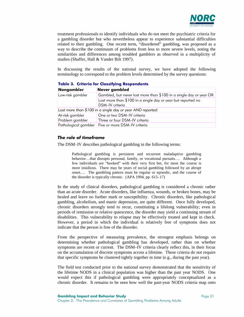
*DPEOLQJ�,PSDFW�DQG�%HKDYLRU�6WXG\ 3DJH���&KDSWHU�����7KH�3UHYDOHQFH�DQG�&RUUHODWHV�RI�*DPEOLQJ�3UREOHPV�$PRQJ�$GXOWV
treatment professionals to identify individuals who do not meet the psychiatric criteria fora gambling disorder but who nevertheless appear to experience substantial difficultiesrelated to their gambling. One recent term, “disordered” gambling, was proposed as away to describe the continuum of problems from less to more severe levels, noting thesimilarities and differences among troubled gamblers as observed in a multiplicity ofstudies (Shaffer, Hall & Vander Bilt 1997).
In discussing the results of the national survey, we have adopted the followingterminology to correspond to the problem levels determined by the survey questions:
7DEOH�����&ULWHULD�IRU�&ODVVLI\LQJ�5HVSRQGHQWV1RQJDPEOHU 1HYHU�JDPEOHG
*DPEOHG��EXW�QHYHU�ORVW�PRUH�WKDQ������LQ�D�VLQJOH�GD\�RU�\HDU�25/RZ�ULVN�JDPEOHU/RVW�PRUH�WKDQ������LQ�D�VLQJOH�GD\�RU�\HDU�EXW�UHSRUWHG�QR'60²,9�FULWHULD
/RVW�PRUH�WKDQ������LQ�D�VLQJOH�GD\�RU�\HDU�$1'�UHSRUWHG�$W�ULVN�JDPEOHU 2QH�RU�WZR�'60²,9�FULWHULD3UREOHP�JDPEOHU 7KUHH�RU�IRXU�'60²,9�FULWHULD3DWKRORJLFDO�JDPEOHU )LYH�RU�PRUH�'60²,9�FULWHULD
7KH�UROH�RI�WLPHIUDPHThe DSM–IV describes pathological gambling in the following terms:
Pathological gambling is persistent and recurrent maladaptive gamblingbehavior…that disrupts personal, family, or vocational pursuits…. Although afew individuals are “hooked” with their very first bet, for most the course ismore insidious. There may be years of social gambling followed by an abruptonset.… The gambling pattern must be regular or episodic, and the course ofthe disorder is typically chronic. (APA 1994, pp. 615–17)
In the study of clinical disorders, pathological gambling is considered a chronic ratherthan an acute disorder. Acute disorders, like influenza, wounds, or broken bones, may behealed and leave no further mark or susceptibility. Chronic disorders, like pathologicalgambling, alcoholism, and manic depression, are quite different. Once fully developed,chronic disorders strongly tend to recur, constituting a lifelong vulnerability; even inperiods of remission or relative quiescence, the disorder may yield a continuing stream ofdisabilities. This vulnerability to relapse may be effectively treated and kept in check.However, a period in which the individual is relatively free of symptoms does notindicate that the person is free of the disorder.
From the perspective of measuring prevalence, the strongest emphasis belongs ondetermining whether pathological gambling has developed, rather than on whethersymptoms are recent or current. The DSM–IV criteria clearly reflect this, in their focuson the accumulation of discrete symptoms across a lifetime. These criteria do not requirethat specific symptoms be clustered tightly together in time (e.g., during the past year).
The field test conducted prior to the national survey demonstrated that the sensitivity ofthe lifetime NODS in a clinical population was higher than the past year NODS. Onewould expect this if pathological gambling were appropriately conceptualized as achronic disorder. It remains to be seen how well the past-year NODS criteria map onto

*DPEOLQJ�,PSDFW�DQG�%HKDYLRU�6WXG\ 3DJH���&KDSWHU�����7KH�3UHYDOHQFH�DQG�&RUUHODWHV�RI�*DPEOLQJ�3UREOHPV�$PRQJ�$GXOWV
clinical assessments of pathological gambling. Based on how the NODS is constructed,as well as our findings in the general population, we believe that the specificity of theNODS items is very good, reducing the rate of lifetime false positives; in this respect, webelieve the performance of the NODS exceeds that of the SOGS.
3DWURQ�6XUYH\
It was expected (and the results below confirm) that the adult RDD survey would yield arelatively small number of cases of pathological and problem gamblers. In anticipationof this limitation, NORC was charged with conducting a second survey to generateadditional problem and pathological gamblers. An intercept survey of patrons of gamingfacilities was selected as the most promising approach—in other words, to go wheregamblers are, and especially where more frequent gamblers would be found inconcentrated numbers. The research design called for 500 patron interviews to becollected from 5 major facility types in approximate proportion to their estimated share inoverall gaming revenues. This distribution was targeted as follows: 170 interviews inlottery ticket outlets (not including locations with video lottery terminals only), 125 inNevada and New Jersey casinos, 65 in riverboat casinos, 65 in Indian reservation casinos,40 in pari-mutuel locations, and 40 in locations with video lottery terminals.
NORC first carried out a pilot study, which comprised 86 interviews with randomlyselected patrons at three destination-style casinos in Wisconsin and Nevada. This type offacility was viewed as the most difficult in which to successfully conduct such a survey.(These casinos agreed to participate in the pilot study through the offices of the NationalIndian Gaming Association and the American Gaming Association.)
The pilot survey provided experience with the process of recruiting sites to participate inthe survey, as well as with some of the specific methodological features of randomlyintercepting and recruiting patrons in these settings (generally in the stream of foot trafficexiting through access doors or corridors), including the feasibility of completing aninterview of this length. We shortened the RDD survey instrument by about one-third, to191 items, to take on average 18 minutes to administer. In addition, the order ofquestions was revised somewhat for ease of administration in a paper-and-pencil in-person format. The field-test interviews were administered by NORC field interviewers.
Finally, in addition to testing the methods of the patron intercept survey, the pilot studyprovided confirmation of the expectation that proportionately greater numbers ofpathological and problem gamblers might be obtained though this type of survey.Although the pilot survey was too small to confirm this point with counts of these twocategories alone, the proportion of at-risk, problem, and pathological gamblers combinedwas nearly 36 percent in the pilot survey—a much richer concentration of such gamblersthan was obtained in the pilot RDD survey.
The design for the patron intercept survey originally called for rotating the periods of datacollection throughout business hours, picking 32 data collection sites with 16 interviewsper site. The tight schedule for completion of the patron intercept survey, onceCommission authorization was obtained, as well as the need to deploy interviewresources efficiently, necessitated a revised design. Therefore, we selected fewer sites,took a greater number of cases per site, and standardized the time frames to the busiest

*DPEOLQJ�,PSDFW�DQG�%HKDYLRU�6WXG\ 3DJH���&KDSWHU�����7KH�3UHYDOHQFH�DQG�&RUUHODWHV�RI�*DPEOLQJ�3UREOHPV�$PRQJ�$GXOWV
hours of mid-afternoon and mid-evening. At the conclusion of the patron interceptsurvey, we had completed 530 interviews in 21 facilities (see Table 4).
7DEOH�����3DWURQ�,QWHUYLHZV
7\SH�RI�)DFLOLW\ 7DUJHWHG $WWHPSWHG &RPSOHWHG5HVSRQVH5DWH
&DVLQRV�LQ�19��1- ��� ��� ��� ���5LYHUERDW�FDVLQRV �� ��� �� ���7ULEDO�FDVLQRV �� �� �� ���/RWWHU\��WUDGLWLRQDO��9/7� ��� ��� ��� ���3DUL�PXWXHO �� ��� �� ���
727$/ ��� ����� ��� ���
The sample facilities were in 7 states from all regions of the country: 4 in the Northeast,with 106 completed interviews; 7 in the North Central region, with 160 interviews; 4 inthe South/Southwest, with 110 interviews; and 6 on the West Coast, with 145 interviews.
The patron intercept data were intended as a supplement to the adult telephone survey.Due to the constraints of sample selection and size, the intention was not to view thesecases in isolation but to analyze them, to the extent possible, together with the telephonecases, improving the overall precision of our information about frequent players andproblem and pathological gamblers. After carefully studying the composition of thepatron intercept sample, we arrived at a procedure to combine the samples and re-weightthe resulting larger file to accurately reflect the “dual-frame” origin of the respondents(that is, we viewed all adults as having two opportunities to be represented in thesample—to be contacted at home via telephone, and to be intercepted while visiting agaming facility). We combined the samples by creating a file that included all of themore frequent past-year lottery or casino players from both surveys (intercept patrons notinterviewed in casino or lottery sites were included here if they met either the lottery orcasino participation criteria in their questionnaire responses). This “players” samplecontained about 1,226 individuals (450 from the patron intercept survey and theremainder from the telephone survey) representing about 64 million players.
We then sorted the players from both surveys into 23 groups or “adjustment cells”(described in more detail in Appendix B); each cell included respondents who reportedsimilar frequencies of casino and lottery play and were similar in age. We then took thepopulation estimated to have the characteristics of each of these cells according to thetelephone data alone and divided that population number by the number of patron ANDtelephone cases in the cell. We then assigned this average weight to each of the patroncases, and finally readjusted all the weights to add up once again to the cell’s population.In other words, we had the intercepted patrons share the sample weights assigned initiallyto the telephone cases whom they most resembled in terms of age and past-year gamblingbehavior. Finally, we recombined these re-weighted cases with all of the telephone caseswho were not in the “players” file; none of these other caseweights (adding up to 133million persons) were changed.
The following table indicates key characteristics of the weighted RDD file, the originalunweighted patron file, and the combined, reweighted patron+RDD file.
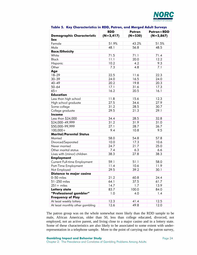
*DPEOLQJ�,PSDFW�DQG�%HKDYLRU�6WXG\ 3DJH���&KDSWHU�����7KH�3UHYDOHQFH�DQG�&RUUHODWHV�RI�*DPEOLQJ�3UREOHPV�$PRQJ�$GXOWV
7DEOH�����.H\�&KDUDFWHULVWLFV�LQ�5''��3DWURQ��DQG�0HUJHG�$GXOW�6XUYH\V
'HPRJUDSKLF�&KDUDFWHULVWLF5''
�1 ������3DWURQ�1 ����
3DWURQ�5''�1 ������
6H[)HPDOH ����� ����� �����0DOH ���� ���� ����5DFH�(WKQLFLW\:KLWH ���� ���� ����%ODFN ���� ���� ����+LVSDQLF ���� ��� ���2WKHU ��� ��� ���$JH��²�� ���� ���� ������²�� ���� ���� ������²�� ���� ���� ������²�� ���� ���� ������� ���� ���� ����(GXFDWLRQ/HVV�WKDQ�KLJK�VFKRRO ���� ���� ����+LJK�VFKRRO�JUDGXDWH ���� ���� ����6RPH�FROOHJH ���� ���� ����&ROOHJH�JUDGXDWH ���� ���� ����,QFRPH/HVV�WKDQ�������� ���� ���� �����������²������ ���� ���� �����������²������ ���� ���� ������������ ��� ���� ���0DULWDO�3DUHQWDO�6WDWXV0DUULHG ���� ���� ����'LYRUFHG�6HSDUDWHG ���� ���� ����1HYHU�PDUULHG ���� ���� ����2WKHU�PDULWDO�VWDWXV ��� ��� ���/LYHV�ZLWK��PLQRU��FKLOGUHQ ���� ���� ����(PSOR\PHQW&XUUHQW�)XOO�WLPH�(PSOR\PHQW ���� ���� ����3DUW�7LPH�(PSOR\PHQW ���� ���� ����1RW�(PSOR\HG ���� ���� ����'LVWDQFH�WR�PDMRU�FDVLQR�²���PLOHV ���� ���� ������²����PLOHV ���� ���� ���������PLOHV ���� ��� ����/RWWHU\�VWDWH ���� ����� ����´3URIHVVLRQDO�JDPEOHUµ ��� ��� ���)UHTXHQF\�RI�3OD\$W�OHDVW�ZHHNO\�ORWWHU\ ���� ���� ����$W�OHDVW�PRQWKO\�RWKHU�JDPEOLQJ ���� ���� ����
The patron group was on the whole somewhat more likely than the RDD sample to bemale, African American, older than 50, less than college educated, divorced, notemployed, not an active parent, and living close to a major casino and in a lottery state.Some of these characteristics are also likely to be associated to some extent with under-representation in a telephone sample. More to the point of carrying out the patron survey,

*DPEOLQJ�,PSDFW�DQG�%HKDYLRU�6WXG\ 3DJH���&KDSWHU�����7KH�3UHYDOHQFH�DQG�&RUUHODWHV�RI�*DPEOLQJ�3UREOHPV�$PRQJ�$GXOWV
the patrons were three to four times more likely to play the lottery at least once a week,gamble in other venues at least once a month, and (albeit only a small fraction) considerthemselves to be “professional” gamblers.
3UHYDOHQFH�5DWHV
Prevalence rates are based on the proportion of respondents who score on increasingnumbers of items that make up the lifetime scale used in the survey. Table 6 presentsinformation about the proportion of respondents who scored at particular levels on thelifetime NODS screen in the RDD survey, the patron survey, and the combined sample(which pools past-year casino and lottery players from the patron survey). Theclassifications, as discussed above, are nongamblers, low-risk gamblers (limitedgambling losses or zero DSM–IV problem criteria), at-risk gamblers (affirmed one or twocriteria), problem gamblers (affirmed three or four criteria), or pathological gamblers(affirmed five or more criteria).
As we display in Table 6, about one in seven (or 29 million) adults have never gambled,and about 148 million adults are low-risk gamblers. At the other end of the spectrum arepathological gamblers, who comprise about 0.8 percent of the adult population based onthe RDD sample alone. Problem gamblers comprise another 1.3 percent of the adultpopulation, based on the RDD sample, and 1.5 percent based on the combined sample.Our best estimate based on the combined sample is that there are about 2½ millionpathological gamblers, 3 million problem gamblers, and 15 million at-risk gamblers inthe United States.
7DEOH�����3HUFHQWDJH�*DPEOLQJ�7\SHV�%DVHG�RQ�/LIHWLPHDQG�3DVW�<HDU�12'6�6FRUHV
5''�6XUYH\ 3DWURQ�6XUYH\&RPELQHG
�3DWURQ�5''�� 1 � 1 � 1
/LIH�WLPH
3DVW<HDU
/LIH�WLPH
3DVW<HDU
/LIH�WLPH
3DVW<HDU
/LIH�WLPH
3DVW
<HDU
/LIH�WLPH
3DVW<HDU
/LIH�WLPH
3DVW<HDU
727$/ ����� ����� ����� ����� ����� ����� ��� ��� ����� ����� ����� �����1RQJDPEOHU ���� ���� ��� ��� ��� ��� � �� ���� ���� ��� ���/RZ�5LVN ���� ���� ����� ����� ���� ���� ��� ��� ���� ���� ����� �����$W�5LVN ��� ��� ��� �� ���� ���� �� �� ��� ��� ��� ���3UREOHP ��� ��� �� � ��� ��� �� �� ��� ��� �� ��3DWKRORJLFDO ��� ��� �� � ��� ��� �� �� ��� ��� �� ��
The higher rates of at-risk, problem, and pathological gambling in the patron surveyconfirm the expectations of the patron pilot survey, although that survey was carried outonly in casinos.
4
4 The division of gambling types among patrons at particular types of gambling facilities was a particular
interest of the Commission. As the table below indicates, the sample sizes, as well as the small number ofsites for each detailed facility type within the patron database, render hazardous any attempt to generalize

*DPEOLQJ�,PSDFW�DQG�%HKDYLRU�6WXG\ 3DJH���&KDSWHU�����7KH�3UHYDOHQFH�DQG�&RUUHODWHV�RI�*DPEOLQJ�3UREOHPV�$PRQJ�$GXOWV
As in other surveys, prevalence rates in the national survey are different among the varioussubgroups of the population. Table 7 shows lifetime prevalence of gambling type bydemographic characteristics in both the RDD and combined surveys.
7DEOH�����/LIHWLPH�DQG�3DVW�<HDU�3UHYDOHQFH�RI�*DPEOLQJ�3UREOHPV�$PRQJ'HPRJUDSKLF�*URXSV��LQ�3HUFHQWDJHV
5''�6XUYH\���� 5''�3DWURQ�6XUYH\����$W�5LVN�Q ����
3UREOHP�Q ���
3DWK��Q ���
$W�5LVN�Q ����
3UREOHP�Q ���
3DWK��Q ���'HPRJUDSKLF
&KDUDFWHULVWLF /LIH�<HDU /LIH�<HDU /LIH�<HDU /LIH�<HDU /LIH�<HDU /LIH�<HDU*HQGHU0DOH ��������� ��������� ��������� ��������� ��������� ���������)HPDOH ��������� ��������� ��������� ��������� ��������� ���������
5DFH:KLWH ��������� ��������� ��������� ��������� ��������� ���������%ODFN ��������� ��������� ��������� ��������� ��������� ���������+LVSDQLF ���������� ��������� ��������� ���������� ��������� ���������2WKHU ��������� ��������� ��������� ��������� ��������� ���������
$JH
from the patron data alone. On a self-weighted basis, 13.2 percent of the patrons interviewed were problemor pathological gamblers, and 17.9 percent were at-risk gamblers. The pari-mutuel patrons at the three race-tracks visited by interviewers differed significantly from the other five types in their distribution of gamblingtypes; there were no statistically significant differences among the first five facility types. The past-yearNODS distributions were very similar to the lifetime but at lower levels: 10.2 percent of all patrons wereproblem or pathological gamblers, and 14.3 percent were at-risk gamblers; across the six facility types fromNevada/Atlantic City casinos to pari-mutuel, pathological and problem gamblers were 6.7, 14.1, 10.5, 6.1,6.7, and 28.5 percent of patrons, respectively.
On a more generalizable basis, patterns of lifetime prevalence were calculated using the combinedRDD+Patron data file for past-year patrons (more than one visit) of Nevada and Atlantic City casinos,riverboats, tribal casinos, traditional lottery outlets, stores/bars restaurants with VLTs or other electronicdevices, and pari-mutuel racetracks. The percentages of pathological and problem gamblers at these siteswere, respectively, 8.5, 9.6, 7.7, 3.8, 5.3, and 15.1 percent. These results indicate that, among the mostcommon gambling venues, multi-visit lottery patrons in general have the lowest prevalence of pathologicaland problem gambling; casino patrons have higher prevalence rates, with small differences by type of casino;and pari-mutuel patrons have the highest prevalence rates.
7DEOH�D���3HUFHQWDJH�RI�*DPEOLQJ�7\SHV�%DVHG�RQ�12'6�/LIHWLPH�6FRUH��E\*DPEOLQJ�9HQXH³3DWURQ�'DWD�2QO\
19�$&�&DVLQR���� 5LYHUERDWV���� 7ULEDO�&DVLQR����7\SH�RI*DPEOHU � 1 � 1 � 1
727$/ ������ ��� ������ �� ������ ��
1RQJDPEOHU ��� � � � � �
/RZ�5LVN ���� ��� ���� �� ���� ��
$W�5LVN ���� �� ���� �� ���� ��
3UREOHP ��� � ��� � ��� �
3DWKRORJLFDO ��� � ���� � ��� �
/RWWHU\�2XWOHWV���� 9/7�/RFDWLRQV���� 3DUL�0XWXHO����7\SH�RI*DPEOHU � 1 � 1 � 1
727$/ ������ ��� ������ �� ������ ��
1RQJDPEOHU � � � � ��� �
/RZ�5LVN ���� ��� ���� �� ���� ��
$W�5LVN ���� �� ���� � ���� ��
3UREOHP ��� � ��� � ���� �
3DWKRORJLFDO ��� � ��� � ���� ��

*DPEOLQJ�,PSDFW�DQG�%HKDYLRU�6WXG\ 3DJH���&KDSWHU�����7KH�3UHYDOHQFH�DQG�&RUUHODWHV�RI�*DPEOLQJ�3UREOHPV�$PRQJ�$GXOWV
7DEOH�����/LIHWLPH�DQG�3DVW�<HDU�3UHYDOHQFH�RI�*DPEOLQJ�3UREOHPV�$PRQJ'HPRJUDSKLF�*URXSV��LQ�3HUFHQWDJHV
5''�6XUYH\���� 5''�3DWURQ�6XUYH\����$W�5LVN�Q ����
3UREOHP�Q ���
3DWK��Q ���
$W�5LVN�Q ����
3UREOHP�Q ���
3DWK��Q ���'HPRJUDSKLF
&KDUDFWHULVWLF /LIH�<HDU /LIH�<HDU /LIH�<HDU /LIH�<HDU /LIH�<HDU /LIH�<HDU��²�� ���������� ��������� ��������� ���������� ��������� �����������²�� ��������� ��������� ��������� ��������� ��������� �����������²�� ��������� ��������� ��������� ��������� ��������� �����������²�� ��������� ��������� ��������� ��������� ��������� ������������ ��������� ��������� ��������� ��������� ��������� ���������
(GXFDWLRQ/HVV�WKDQ�+6 ���������� ��������� ��������� ���������� ��������� ���������+6�JUDGXDWH ��������� ��������� ��������� ��������� ��������� ���������6RPH�FROOHJH ��������� ��������� ��������� ��������� ��������� ���������&ROOHJH�JUDGXDWH ��������� ��������� ��������� ��������� ��������� ���������
,QFRPH/HVV�WKDQ�������� ��������� ��������� ��������� ��������� ��������� ����������������²������ ��������� ��������� ��������� ��������� ��������� ����������������²������ ��������� ��������� ��������� ��������� ��������� ������������������ ���������� ��������� ��������� ���������� ��������� ���������
0DULWDO�VWDWXV0DUULHG ��������� ��������� ��������� ��������� ��������� ���������'LYRUFHG�VHSDUDWHG ��������� ��������� ��������� ��������� ��������� ���������1HYHU�PDUULHG ���������� ��������� ��������� ���������� ��������� ���������&RKDELWLQJ ��������� ��������� ��������� ��������� ��������� ���������:LGRZHG ��������� ��������� ��������� ��������� ��������� ���������
0LQRU�FKLOGUHQ1RQH ��������� ��������� ��������� ��������� ��������� ���������2QH�RU�PRUH ��������� ��������� ��������� ��������� ��������� ���������
(PSOR\PHQW)XOO�WLPH ��������� ��������� ��������� ��������� ��������� ���������3DUW�WLPH ��������� ��������� ��������� ��������� ��������� ���������1RW�HPSOR\HG ��������� ��������� ��������� ��������� ��������� ���������
5HJLRQ1RUWKHDVW ���������� ��������� ��������� ��������� ��������� ���������6RXWK ��������� ��������� ��������� ��������� ��������� ���������0LGZHVW ��������� ��������� ��������� ��������� ��������� ���������:HVW ���������� ��������� ��������� ���������� ��������� ���������
/RWWHU\�VWDWH1R ��������� ��������� ��������� ��������� ��������� ���������<HV ��������� ��������� ��������� ��������� ��������� ���������
'LVWDQFH�WR�FDVLQR�²���PLOHV ��������� ��������� ��������� ��������� ��������� �����������²����PLOHV ��������� ��������� ��������� ��������� ��������� ������������� ��������� ��������� ��������� ��������� ��������� ���������
3URIHVVLRQDO�JDPEOHU1R ��������� ��������� ��������� ��������� ��������� ���������<HV ���������� �������� ���������� ��������� ��������� ���������
*DPEOLQJ�,PSDFW�DQG�%HKDYLRU�6WXG\ 3DJH���&KDSWHU�����7KH�3UHYDOHQFH�DQG�&RUUHODWHV�RI�*DPEOLQJ�3UREOHPV�$PRQJ�$GXOWV
Several interesting observations can be made based on this table and associated tests ofstatistical significance (every specific difference in our findings that is noted in thefollowing discussion has a 5 percent or less likelihood of arising by chance). First, withregard to sex, we found that prevalence rates of problem and pathological gamblingtended to be higher among men than women in the RDD survey, but not to statisticalsignificance. However, significantly more at-risk male gamblers were present in thissample than at-risk female gamblers. When we increased the sample size by merging theRDD and patron survey data, analysis revealed that rates of at-risk, problem, andpathological gambling were all higher among men.
When we examined differences by age, we found that persons 65 years and older weresubstantially less likely to be at-risk, problem, or pathological gamblers than those inyounger age groups. The prevalence rates of at-risk, problem, and pathological gamblingare also higher among African Americans than whites in the combined survey (thedifference in the RDD survey reaches significance only for pathological gamblers). Inthe combined survey data, the prevalence of at-risk and problem gambling is higheramong the never married than those who are married, and divorced people have higherprevalence rates of pathological, problem, and at-risk gambling than married people.Prevalence is higher among respondents living with minor children in the household thanamong those without minor children in the household, but this may be due to the differentage and sex profile of people living with minors (more of whom are women and under65) versus those who are not.
Finally, about 1 percent of respondents in the telephone survey identified themselves as“professional gamblers.” Problem and pathological gambling are both present at elevatedrates in this group. The DSM–IV states that professional gamblers, who limit their risk-taking and gamble in a “disciplined” way may relate somewhat differently to thescreening items than other gamblers. However, the DSM–IV does not suggest thatprofessionals are immune to gambling problems, any more than professional bartendersare immune to alcohol problems; nor does the DSM–IV recommend (or have a basis torecommend) that the screening criteria be modified for this subgroup. The evidence ofour survey suggests that persons who consider themselves professional gamblers do notnecessarily earn their entire living or even a significant part of it by gambling.
5HJLRQDO�'LIIHUHQFHV�DQG�$YDLODELOLW\
In summarizing the results of a large number of prevalence studies conducted throughoutthe United States, Cox, Lesieur, Rosenthal, and Volberg (1997) noted that prevalencerates tend to be lowest in the Midwest and higher in the Northeast. This cross-jurisdictional analysis also showed that prevalence rates are highest in southern states likeLouisiana and Mississippi, where the availability of legal gambling has increased rapidly,where the population is ethnically diverse, and where socioeconomic levels are relativelylow. In the national survey, prevalence rates of pathological and problem gambling arelowest in the Northeast and highest in the West.
The availability of a state-owned lottery has a statistically significant association with theprevalence of at-risk gambling (which increases about 80 percent, in parallel with thegenerally greater past-year lottery play in these states, 55 percent versus 33 percent).However, the difference in prevalence of problem and pathological gamblers hovers atthe edge of statistical significance, and is in the opposite direction. The availability of a

*DPEOLQJ�,PSDFW�DQG�%HKDYLRU�6WXG\ 3DJH���&KDSWHU�����7KH�3UHYDOHQFH�DQG�&RUUHODWHV�RI�*DPEOLQJ�3UREOHPV�$PRQJ�$GXOWV
casino within 50 miles (versus 50–250 miles) is associated with a higher prevalence(about double) of problem and pathological gambling in the combined survey results,parallel with the general difference in levels of past-year casino gambling (40 percentamong adults within 50 miles, vs. 23 percent of adults 50–150 miles). However, wefound little difference in the prevalence of at-risk gambling in the combined survey, anddifferences in prevalence were not statistically significant in the RDD survey.
$WWLWXGHV�7RZDUG�*DPEOLQJ
It is interesting to examine general attitudes toward gambling among problem andpathological gamblers. One might assume that despite their gambling-related difficulties,problem and pathological gamblers enjoy gambling and believe that it is generally a goodthing for society. However, Table 8 shows that nearly half of all pathological gamblers,as identified by lifetime NODS scores, believe that the overall effect of legalizedgambling on society is either bad or very bad; these attitudes are more negative than forany other group of gamblers. When the smaller groups with positive past-year NODSscores are examined, gamblers at every problem level are less negative about the impactof gambling (conversely, the group that did not gamble in the past year is much largerthan just the lifetime nongamblers, and generally more negative about gambling).
Respondents in the national survey were also asked about their reasons for gambling.Table 8 shows that the majority of at-risk, problem, and pathological gamblers gamblefor excitement or challenge, and in this respect are quite different from low-riskgamblers. A great majority of at-risk, problem, and pathological gamblers also gamble inorder to win money, and in this respect they also differ from low-risk gamblers. Finally,we found no statistically significant differences among these groups in the extent towhich they gamble with friends or family, except that pathological gamblers exceedothers. All of these results are the same whether the past-year or lifetime NODS is used.
7DEOH�����$WWLWXGHV�7RZDUG�*DPEOLQJ�LQ�5''�3DWURQ�6XUYH\��E\�/LIHWLPH�DQG3DVW�<HDU�*DPEOHU�7\SH
/RZ�5LVN $W�5LVN3UREOHP*DPEOHUV
3DWK�*DPEOHUV
$WWLWXGH�7RZDUG�*DPEOLQJ /LIH�<HDU /LIH�<HDU /LIH�<HDU /LIH�<HDU2YHUDOO�LPSDFW�LV�EDG�YHU\�EDG �������� �������� �������� ��������([FLWHPHQW�LV�LPSRUWDQW�YHU\�LPS ������� ������� ������� �������:LQQLQJ�PRQH\�LPSRUWDQW�YHU\�LPS ������� ������� ������� �������8VXDOO\�JDPEOH�ZLWK�IULHQGV��IDPLO\ ������� ������� ������� �������
&RUUHODWLRQ�ZLWK�2WKHU�'LVRUGHUV
Finally, it is useful to compare problem and pathological gamblers to others in thenational survey in terms of physical and psychological disorders and other kinds oftroubles in life. Table 9 shows the percentages of gamblers and nongamblers who haveexperienced some of these problems. Lifetime pathological gamblers are twice as likelyas other gamblers (31 percent versus about 15 percent, with nongamblers, an older group,falling in between) to describe their general health over the past 12 months as fair orpoor. Lifetime pathological and problem gamblers are twice as likely as all other groups(13 percent versus 6 to 7 percent) to have sought professional help for emotional or

*DPEOLQJ�,PSDFW�DQG�%HKDYLRU�6WXG\ 3DJH���&KDSWHU�����7KH�3UHYDOHQFH�DQG�&RUUHODWHV�RI�*DPEOLQJ�3UREOHPV�$PRQJ�$GXOWV
mental health problems in the past year. Lifetime pathological and problem gamblers aremore likely than at-risk gamblers (42 percent, versus 27 percent) to acknowledge beingsomewhat or very troubled by their emotions, nerves or mental health; lifetime at-riskgamblers are in turn more likely than lifetime low-risk gamblers (16 percent), who aremore likely than persons who have never gambled (11 percent) to affirm this.
7DEOH�����3HUFHQWDJH�RI�/LIHWLPH�DQG�3DVW�<HDU�*DPEOHU�7\SHV�E\�+HDOWK��0HQWDO+HDOWK��6XEVWDQFH�$EXVH��DQG�2WKHU�3UREOHPV
1RQ�JDPEOHUV
/RZ�5LVN*DPEOHUV
$W�5LVN*DPEOHUV
3UREOHP*DPEOHUV
3DWK�*DPEOHUV
3UREOHP/LIH�WLPH
3DVW<HDU
/LIH�WLPH
3DVW<HDU
/LIH�WLPH
3DVW<HDU
/LIH�WLPH
3DVW<HDU
/LIH�WLPH
3DVW<HDU
+HDOWK�SRRU�IDLU��SDVW�\HDU ���� ���� ���� ���� ���� ���� ���� ���� ���� ����0HQWDOO\�WURXEOHG��FXUUHQWO\��5''�RQO\�
���� ���� ���� ���� ���� ���� ���� ���� ���� ����
0HQWDO�KHDOWK�W[��SDVW�\HDU ��� ��� ��� ��� ��� ���� ���� ��� ���� ����(PRWLRQDOO\�KDUPIXO�IDPLO\DUJXPHQW�DERXW�JDPEOLQJ
1$ ��� ��� ��� ��� ��� ���� ���� ���� ����
0DQLF�V\PSWRPV��HYHU 1$ ��� 1$ ��� ���� ���� ���� ���� ���� ����'HSUHVVLYH�HSLVRGH��HYHU�5''�RQO\�
1$ ��� 1$ ��� ��� ���� ���� ��� ���� ����
$OFRKRO�GUXJ�GHSHQGHQW��HYHU�5''�RQO\�
��� ��� ��� ��� ��� ���� ���� ���� ��� ����
'UXJ�XVH����GD\V��SDVW�\HDU ��� ��� ��� ��� ��� ���� ���� ���� ��� ����$Q\�MRE�ORVV��SDVW�\HDU ��� ��� ��� ��� ��� ��� ���� ��� ���� ����%DQNUXSWF\��HYHU ��� ��� ��� ��� ��� ���� ���� ���� ���� ����$UUHVWHG��HYHU ��� ��� ���� ���� ���� ���� ���� ���� ���� ����,QFDUFHUDWHG��HYHU��5''�RQO\� ��� ³ ��� ³ ��� ³ ���� ³ ���� ³
The survey questionnaire includes screens for manic or depressive episodes, that is,questions asking whether a respondent ever displayed certain symptoms that are stronglyindicative of manic or depressive episodes. The depression items led, if answeredpositively, to a full series of DSM–IV diagnostic questions, but this series was only usedwith respondents scoring one or more points on the NODS; other national surveysestimate general prevalence with the same questions. The manic screening items wereasked only of respondents who scored one or more points on the NODS. This helps shedfurther light on the “manic episode” exclusion for the psychiatric disorder of pathologicalgambling, but we do not attempt to implement this exclusion. It has not beenimplemented in previous studies using the DSM–IV criteria, nor is there an underlyingresearch base to indicate how it would be implemented, and therefore no research tovalidate an exclusion procedure (Lesieur and Rosenthal, 1998).
Table 9 shows that lifetime and past year pathological gamblers are significantly morelikely than other risk respondents to have symptoms associated with manic disorder. Thelifetime prevalence of major depressive episode among problem and pathologicalgamblers is significantly higher than that observed in the general population in othersurveys, and a definite downward trend is noted from those with the most to least severegambling problems in our sample. Table 9 also shows that both lifetime and past-yearrespondents reporting at-risk, problem, and pathological gambling are more likely than

*DPEOLQJ�,PSDFW�DQG�%HKDYLRU�6WXG\ 3DJH���&KDSWHU�����7KH�3UHYDOHQFH�DQG�&RUUHODWHV�RI�*DPEOLQJ�3UREOHPV�$PRQJ�$GXOWV
low-risk or nongamblers to have ever been alcohol or drug-dependent and to have usedillicit drugs in the past 12 months. Lifetime , as well as to have ever been arrested orincarcerated. Finally, pathological and problem gamblers are more likely than any othergroup to have lost a job in the past year and to have ever declared bankruptcy.
*DPEOLQJ�([SHQGLWXUHV
One expectation of our survey work was that it would enable us to estimate theproportion of gaming revenues associated with problem and pathological gamblers.There are two principal obstacles to this enterprise. First, a certain fraction of gamingrevenues, particularly in destination-style casinos but also in certain high-stakes lotteries,have historically been derived from a relatively small number of high-end players, manyof whom are not U.S. residents. Therefore, estimates based on a survey that does notsample from this special stratum must restrict its scope of generalization to excludereference to these very wealthy players. Because these players are so few in number,determination of the population prevalence and correlates of problem and pathologicalgambling are not affected by their absence from the survey. However, due to the amountof money that these individuals put into play at casinos (and to an evidently much lesserextent in other games), any denomination of gambling in monetary units will be missingthis component.
The second problem is the weakness in individuals’ reports of gambling winnings andlosses. Virtually none of the survey data on the reported amounts “ahead” or “behind”(won or lost) appears to be accurate at face value, when compared with official statisticaldata on regulated games. An exception is lottery play, for which we were able toreconcile the survey data quite well with officially counted sales receipts. This exceptionis probably due to the more routinized purchase patterns of most lottery play, comparedwith the way that betting and payoffs take place in other games with faster, morecomplicated, and more interactive formats. But here as well, the net win/loss data varyappreciably from what ticket buyers are known to spend and not recover through winningtickets. Instead of a careful, computer-like accounting for gaming dollars, individualstend to understate their net losses and exaggerate their net wins, particularly whenaccounting for expenditures in private settings.
Table 10, which is based on the RDD questionnaire data (which covered gambling winsand losses much more extensively than the patron questionnaire; but see footnote 4below), displays gambling win, loss, and expenditure totals for five types of gambling, intotal and by type of gambler. The table provides numerous instances of non-credibleoverall results—for example, the results of adding up reports of lottery ticket purchases,on the one hand (expenditure data), and on the other, how much the survey respondentsthought they were ahead (won) or behind (lost) over the course of a year. The annualinformation is calculated separately from two kinds of questions—items about the lastday the respondent gambled, which are summed up taking account of the reportednumber of days gambling each year, and a direct question about past-year gambling winsor losses.

*DPEOLQJ�,PSDFW�DQG�%HKDYLRU�6WXG\ 3DJH���&KDSWHU�����7KH�3UHYDOHQFH�DQG�&RUUHODWHV�RI�*DPEOLQJ�3UREOHPV�$PRQJ�$GXOWV
7DEOH������(VWLPDWHG�$QQXDO�$PRXQW�$KHDG��%HKLQG��RU�6SHQW��LQ�0LOOLRQV�RI'ROODUV��LQ�WKH�3DVW�<HDU��������IURP�5''�'DWD�
&DVLQR 7UDFN/DVW�'D\�6XPV 3DVW�<HDU /DVW�'D\�6XPV 3DVW�<HDU$KHDG %HKLQG $KHDG %HKLQG $KHDG %HKLQG $KHDG %HKLQG
7RWDO ��������������
��������������
�������������
�������������
�������������
�������������
�������������
�������������
*DPEOHU�W\SH�UHSRUWLQJ�DPRXQW/RZ�5LVN ������
�����������������
�����������
�����������
�����������
�����������
�����������
���������
$W�5LVN �����������
������������
��������
�����������
��������
���������
���������
���������
3UREOHP ����������
�����������
�����������
��������
��������
�������
�������
���������
3DWKRORJLFDO ��������
����������
�������
���������
��������
² ������
�������
3ULYDWH /RWWHU\ 8QOLFHQVHG/DVW�'D\�6XPV 3DVW�<HDU 3DVW�<HDU 3DVW�<HDU$KHDG %HKLQG $KHDG %HKLQG $KHDG %HKLQG 7RWDO�� $KHDG %HKLQG
7RWDO ��������������
�������������
�������������
�����������
�������������
�������������
��������������
�������������
�����������
*DPEOHU�W\SH�UHSRUWLQJ�DPRXQW/RZ�5LVN ������
�����������������
�����������
���������
�����������
�����������
������������
�����������
���������
$W�5LVN �����������
��������
��������
��������
�������
�����������
�����������
���������
���������
3UREOHP ��������
�����������
�����������
������
�������
��������
����������
���������
�������
3DWKRORJLFDO ³ ³ ������
������
³ �������
��������
³ �������
The total spending estimate for lottery tickets using the RDD data only is 25.5 billion.This figure is approximately 20 percent below the national lottery sales figures for 1998sales cited by Clotfelter, Cook, Edell, and Moore (1999) in their analysis of lotterygambling for the Commission.
5 However, to be consistent, the same players in the
survey, when asked to estimate their net receipts, should have reported losses of
5 The combined RDD+patron data on lottery expenditures, in contrast to other data in Table 10, are more
complete than the RDD alone. Using the combined data set, we calculated the total lottery expenditures inthe past year to be $31,5 billion, which is very similar to the figures cited by Clotfelter and colleagues for1998 national lottery sales. However, Clotfelter and colleagues arrived at their own survey-based estimatefor total national expenditures on lottery tickets (based on the same combined data set) by using a morecomplex summing algorithm to quantify the frequency-of-play response categories in the NORCquestionnaire, as well as a series of post hoc adjustment factors designed to match the survey estimates foreach major lottery type with the FY1998 sales figures published by LaFleur (www.lafleurs.com). When weused the same program code (Malme, private communication) to calculate the distribution of expenditures bytype of gambler, we calculated the percentage of the $31.9 billion total expenditure by low-risk, at-risk,problem, and pathological gamblers at 67.5 percent, 18.0 percent, 7.9 percent, and 6.6 percent, respectively—statistics which are very close to our estimates based on the combined data (67.0, 18.8, 7.6, and 6.6) , whichare similar to those in Table 10 except that the RDD data ascribe a much lower percentage of lotteryexpenditures to pathological gamblers.. Further analytic explorations of these data, as well as furthermethodological research on how to elicit the most accurate expenditure information, will undoubtedly proveuseful to students of lottery play.

*DPEOLQJ�,PSDFW�DQG�%HKDYLRU�6WXG\ 3DJH���&KDSWHU�����7KH�3UHYDOHQFH�DQG�&RUUHODWHV�RI�*DPEOLQJ�3UREOHPV�$PRQJ�$GXOWV
approximately $14 billion, reflecting the percentage of lottery expenditures not returnedto ticket-holders. Instead, the data equate to a net loss of $4.7 billion, reflecting $1.4billion in winnings (claimed by about 8 percent of all the past-year players) and $6.1billion in losses (contributed by about 85 percent of players); the remaining 7 percent“broke even.” This loss is about one-third what it should have been based on the survey-expenditures captured in the RDD data, and about one-fourth the actual amount lostaccording to the official sales data.
Undercounting of losses and/or overcounting of winnings are also evident for other formsof gambling, both for wins and losses across the past year as well as on the last dayrespondents gambled. The balance of past-year casino wins and losses for last-day andpast-year items shows patrons ending up with a $5 billion or $3 billion windfall, insteadof leaving more than $20 billion at tables and machines—the revenues reported by thecasino industry. The same reversals hold for tracks and for unlicensed betting, comprisedlargely of sports books.
Most revealing of the rosiness of the collective view of gambling results is privategaming, largely at cards, in which there is no “house” or commercial intermediary toremove money from players’ wins and losses. In private bets, all of the wins and lossesshould balance. However, the last-day-based and past-year aggregates from the surveyshow the amounts won exceeding the amounts lost by factors of seven and twelve,respectively. Unlike lottery play, in which 85 percent of buyers consider themselves netlosers and 8 percent net winners (a 1:10 ratio), in private games, on the last day of playthere were 3 self-reported winners for each loser (3:1), and over a year’s time, fiveoverall winners for every three losers (5:3). While these ratios are not inherentlyimpossible, since they might imply that each losers’ money was spread out across a largernumber of (smaller) winners, the individual amounts reported as won and lost by eachgroup actually greatly exaggerate, rather than reduce, this disparity in numbers of winnersand losers.
Despite the lack of realism in the overall estimates of monetary wins and losses, there issome degree of information in the extent to which problem and pathological gamblersaccount for the amounts in both the win and loss columns (and in the case of lotteries, theexpenditure column). Discounting the impossible sums of conjured winnings in privategames, most of the money actually and reportedly changing hands is in lotteries, casinos,and pari-mutuel betting, and these are the estimates for which the number of respondentsreporting win/loss data are the largest.
In lottery play, problem and pathological gamblers account for 8 percent of totalexpenditures (but 14.2 percent in the combined survey data for this measure), 8.1 percentof past-year losses, and 1.1 percent of past-year winnings. In casino play, problem andpathological gamblers account for 22.1 percent of past-year losses, 14.3. percent of last-day-based losses, 16.8 percent of past-year winnings, and 6.4 percent of last-day-basedgains. In pari-mutuel betting, problem and pathological gamblers account for 15.5percent of past-year losses, 3.3 percent of past-year winnings, none of the last-day-basedlosses, and 1.2 percent of last-day-based winnings..
Overall, when we sum up these data, similar information on the less frequently playedgames, and parallel monetary items such as the amount of money taken to gamble with orhow much the person was willing to lose, these sums converge on the estimate that about

*DPEOLQJ�,PSDFW�DQG�%HKDYLRU�6WXG\ 3DJH���&KDSWHU�����7KH�3UHYDOHQFH�DQG�&RUUHODWHV�RI�*DPEOLQJ�3UREOHPV�$PRQJ�$GXOWV
15 percent of the dollars lost gambling are lost by problem and pathological gamblers.These figures well exceed the percentage of problem and pathological gamblers in thegeneral population, but not by so much as to dominate the economics of gambling.Perhaps a more general finding from these data is that gamblers, whether or not they areclassifiable as problem or pathological, seem accustomed to a fairly high level of wishfulthinking about the economics of the games they play.
$VVHVVLQJ�3UREOHP�DQG�3DWKRORJLFDO�*DPEOLQJ�LQ�WKH�)XWXUH
The issues surrounding legal gambling have become far more complex than they werewhen the last Commission published its report in 1976. Policy makers, governmentagencies, gambling regulators, and gaming operators are concerned about the likely impactsof changing mixes of legal gambling on the gambling behavior of broad segments of thepopulation, as well as on the prevalence of gambling-related difficulties. Public healthresearchers and social scientists are concerned with minimizing the risks of legal gamblingto particular subgroups in the population. Economists, financial institutions, and lawenforcement professionals are concerned about the relationship between legal gambling andbankruptcies, gambling and crime, and the reliance of the gaming industries on problemgamblers for revenues. Treatment professionals, government agencies, and not-for-profitorganizations are concerned about how to allocate scarce resources for the prevention andtreatment of gambling problems (Volberg 1998b). Finally, groups opposed to theexpansion of legal gambling are now working to prevent the further expansion of legalgambling and to repeal existing activities.
Like much of science, measurement is a developmental process. Instrumentation isalways a reflection of the work that researchers are doing to identify and describe thephenomena in which they are interested. As research on problem gambling continues,our systems change for classifying problem gamblers. The SOGS represents a culturallyand historically situated consensus about the nature of gambling problems. As researchcontinues and as the definitions of problem gambling change, new instruments and newmethods for estimating prevalence in the general population and for testing models ofgambling behavior will continue to emerge. These emerging methods must be testedagainst each other and against the SOGS in order to advance the field of problemgambling research in an orderly manner, ensuring the relevance of past work as well aswork in the future.
There are several areas for which we would recommend future research investmentsMuch more work needs to done with the patron intercept methodology as a way tocapture frequent players. This type of survey work requires cooperation betweenresearchers and the gaming industry, which will undoubtedly increase as the importanceand value of onsite research findings becomes more widely understood. Research is alsoneeded on the efficacy of treatment for gambling problems, both through voluntarysupport groups and professional channels. Finally, longitudinal studies are needed thatcan extrapolate across 20-year spans or longer on the “careers” or “natural history” ofgambling and related disorders.

*DPEOLQJ�,PSDFW�DQG�%HKDYLRU�6WXG\ 3DJH���&KDSWHU�����7KH�3UHYDOHQFH�DQG�&RUUHODWHV�RI�*DPEOLQJ�3UREOHPV�$PRQJ�$GXOWV
5HIHUHQFHV
Abbott, M.W. & R.A. Volberg. 1992. Frequent Gamblers and Problem Gamblers inNew Zealand: Report on Phase Two of the National Survey. Research SeriesNo. 14. Wellington: New Zealand Department of Internal Affairs.
Abbott, M.W. & R.A. Volberg. 1996. “The New Zealand National Survey of Problemand Pathological Gambling.” Journal of Gambling Studies, 12 (2): 143–160.
Abt, V. & M.C. McGurrin. 1991. “The Politics of Problem Gambling: Issues in theProfessionalization of Addiction Counseling.” In Gambling and Public Policy:International Perspectives, W.R. Eadington & J.A. Cornelius (eds). Reno:University of Nevada Press. Pp. 657–670.
American Psychiatric Association. 1980. Diagnostic and Statistical Manual ofMental Disorders, Third Edition. Washington, DC: American PsychiatricAssociation.
American Psychiatric Association. 1994. Diagnostic and Statistical Manual ofMental Disorders, Fourth Edition. Washington, DC: American PsychiatricAssociation.
Becker, H.S. 1960. “Notes on the Concept of Commitment,” American Journal ofSociology 66: 32–40.
Cox, S., H. Lesieur, R. Rosenthal & R. Volberg. 1997. Problem and PathologicalGambling in America: The National Picture. Report prepared by the Researchand Public Policy Committees of the National Council on Problem Gambling.
Christiansen, E.M. 1998. “The United States Gross Annual Wager: 1997.”International Gaming & Wagering Business, Supplement, August 1998.
Clotfelter, C.T., Cook, P.J.,. Edell, J.A., & Moore, M. 1999. “State Lotteries at theTurn of the Century: Report to the National Gambling Impact StudyCommission.” Durham, N.C.: Duke University.
Culleton, R.P. 1989. “The Prevalence Rates of Pathological Gambling: A Look atMethods,” Journal of Gambling Behavior 5: 22–41.
Cunningham-Williams, R.M., L.B. Cottler, W.M. Compton & E.L. Spitznagel. 1998.“Taking Chances: Problem Gamblers and Mental Health Disorders: Results fromthe St. Louis Catchment Area (ECA) Study,” American Journal of Public Health88 (7): 1093–1096.
Dean, J. 1979. “Controversy Over Classification: A Case Study From the Historyof Botany.” In Natural Order: Historical Studies of Scientific Culture, B.Barnes & S. Shapin (eds). Beverly Hills, CA: Sage Publications.Dickerson,M.G. 1993. “A Preliminary Exploration of a Two-Stage Methodology in theAssessment of the Extent and Degree of Gambling-Related Problems in theAustralian Population.” In Gambling Behavior and Problem Gambling. W.R.Eadington & J.A. Cornelius (eds). Reno: University of Nevada Press.
Dohrenwend, B.P. 1995. “The Problem of Validity in Field Studies of PsychologicalDisorders, Revisited.” In Ming, T. Tsuang, Mauricio Tohen & Gwendolyn E.P.Zahner (eds), Textbook in Psychiatric Epidemiology. New York: Wiley-Liss.Pp. 3–20.
Dohrenwend, B.P. 1998. “A Psychosocial Perspective on the Past and Future ofPsychiatric Epidemiology,” American Jour of Epidemiology 147 (3): 222–231.

*DPEOLQJ�,PSDFW�DQG�%HKDYLRU�6WXG\ 3DJH���&KDSWHU�����7KH�3UHYDOHQFH�DQG�&RUUHODWHV�RI�*DPEOLQJ�3UREOHPV�$PRQJ�$GXOWV
Fisher, S.E. 1996. Gambling and Problem Gambling Among Casino Patrons.Report to the British Casino Industry Consortium.
Gerson, E.M. 1983. “Scientific Work and Social Worlds,” Knowledge 4: 357–379.
Kallick, M., Suits, D. Dielman, T. & J. Hybels. 1976. Survey of American GamblingAttitudes and Behavior. Research Report Series, Survey Research Center,Institute for Social Research. Ann Arbor: University of Michigan Press.
Lesieur, H.R. 1994. “Epidemiological Surveys of Pathological Gambling: Critiqueand Suggestions for Modification,” Journal of Gambling Studies 10 (4): 385–398.
Lesieur, H.R. & S.B. Blume. 1987. “The South Oaks Gambling Screen (SOGS): ANew Instrument for the Identification of Pathological Gamblers,” AmericanJournal of Psychiatry 144: 1184–1188.
Lesieur, H.R. & S.B. Blume. 1991. “When Lady Luck Loses: Women andCompulsive Gambling.” In Feminist Perspectives on Addictions, Nan van denBergh (ed.). New York: Springer. Pp. 181–197.
Lesieur, H.R. & R.J. Rosenthal. 1991. “Pathological Gambling: A Review of theLiterature (prepared for the American Psychiatric Association Task Force onDSM–IV Committee on Disorders of Impulse Control Not ElsewhereClassified),” Journal of Gambling Studies 7: 5–40.
Lesieur, H.R. & R.J. Rosenthal. 1998. “Analysis of Pathological Gambling.” InT.A. Widiger, A.J. Francis, H.A. Pincus, R. Ross, M.B. First, W. Davis & M.Kline (eds.). DSM–IV Sourcebook. Volume 4. Washington, D.C.: AmericanPsychiatric Association, pp. 393–401.
Polzin, P.E., J. Baldridge, D. Doyle, J.T. Sylvester, R.A. Volberg & W.L. Moore.1998. “From Convenience Stores to Casinos: Gambling–Montana Style.”Montana Business Quarterly 36 (4): 2–14.
Porter, T.M. 1995. Trust in Numbers: The Pursuit of Objectivity in Science andPublic Life. Princeton, NJ: Princeton University Press.
Rosecrance, J. 1985. “Compulsive Gambling and the Medicalization of Deviance,”Social Problems 32: 275–284.
Shaffer, H.J., M.N. Hall & J. Vander Bilt. 1997. Estimating the Prevalence ofDisordered Gambling Behavior in the United States and Canada: A Meta-analysis. Boston, MA: Harvard Medical School Division on Addictions.
Stinchfield, R. 1997. Reliability, Validity and Classification Accuracy of the SouthOaks Gambling Screen (SOGS). Paper presented at the 10th InternationalConference on Gambling and Risk Taking. Montreal, Canada.
Volberg, R.A. 1983. Constraints and Commitments in the Development of AmericanBotany, 1880–1920. Ph.D. Dissertation. University of California, San Francisco.
Volberg, R.A. 1992. Gambling Involvement and Problem Gambling in Montana.Report to the Montana Department of Corrections and Human Services.
Volberg, R.A. 1994. “Assessing Problem and Pathological Gambling in the GeneralPopulation: A Methodological Review.” In Gambling in Canada: The BottomLine, Colin S. Campbell (ed.). Vancouver: Simon Fraser University Press. Pp.137–146.

*DPEOLQJ�,PSDFW�DQG�%HKDYLRU�6WXG\ 3DJH���&KDSWHU�����7KH�3UHYDOHQFH�DQG�&RUUHODWHV�RI�*DPEOLQJ�3UREOHPV�$PRQJ�$GXOWV
Volberg, R.A. 1997a. Gambling and Problem Gambling in Colorado. Report to theColorado Department of Revenue.
Volberg, R.A. 1997b. Gambling and Problem Gambling in Oregon. Report to theOregon Gambling Addiction Treatment Foundation.
Volberg, R.A. 1998a. The Evolution of Gambling in North America. KeynoteAddress, Alberta Lotteries and Gaming Summit. Medicine Hat, Alberta.
Volberg, R.A. 1998b. Testimony: Research on Problem Gambling. Testimonybefore the National Gambling Impact Study Commission. Expert Panel onPathological Gambling. (January 22, 1998).
Volberg, R.A. & S.M. Banks. 1990. “A Review of Two Measures of PathologicalGambling in the United States,” Journal of Gambling Behavior 6(2): 153–163.Volberg, R.A. & M.G. Dickerson (eds.). 1996. Journal of GamblingStudies, Special Issue on International Prevalence Studies and Related TreatmentDevelopments. Vol. 12, No. 2.
Volberg, R.A. & W.L. Moore. 1999. Gambling and Problem Gambling in Sweden.Report to the International Gambling Research Team of Sweden.
Volberg, R.A. & E. Silver. 1993. Gambling and Problem Gambling in NorthDakota. Report to the North Dakota Department of Human Services, Division ofMental Health.
Volberg, R.A. & H.J. Steadman. 1988. “Refining Prevalence Estimates ofPathological Gambling,” American Journal of Psychiatry 145: 502–505.
Volberg, R.A. & H.J. Steadman. 1992. “Accurately Depicting PathologicalGamblers: Policy and Treatment Implications.” Journal of Gambling Studies 8(4): 401–412.
Volberg, R.A. & R.M. Stuefen. 1991. Gambling and Problem Gambling in SouthDakota. Report to the Governor’s Office of South Dakota.Walker, M.B. 1992.The Psychology of Gambling. Oxford: Pergamon Press.
Walker, M.B. & M.G. Dickerson. 1996. “The Prevalence of Problem andPathological Gambling: A Critical Analysis,” Journal of Gambling Studies 12(2): 233–249.
Winters, K.C., S. Specker & R. Stinchfield. 1997. Brief Manual for Use of theDiagnostic Interview for Gambling Severity. Minneapolis, MN: University ofMinnesota Medical School.

*DPEOLQJ�,PSDFW�DQG�%HKDYLRU�6WXG\ 3DJH���&KDSWHU�����(FRQRPLF�$QDO\VLV�RI�&RQVHTXHQFHV�RI�*DPEOLQJ�3UREOHPV�$PRQJ�$GXOWV
&+$37(5�����(&2120,&�$1$/<6,6�2)�7+(�&216(48(1&(6�2)*$0%/,1*�352%/(06�$021*�$'8/76
Problem and pathological gamblers, as defined in previous sections of this report,experience excessive rates of adverse consequences that have tangible economic costs.Further consequences experienced by these gamblers that are quite real (e.g., brokenrelationships and families), although not readily amenable to having price tags attached,are often termed “intangible” costs. Another dimension of gambling consequences is thattheir impact is usually spread across an entire community. While costs begin with thegambler, they spill over to the household, other family members, friends, employers,creditors, and the community as a whole.
The focus of this analysis is on the tangible economic value of gamblers’ problems orconsequences that have been identified and analyzed in the literature on problem andpathological gambling (see, e.g., Lesieur 1998; Volberg et al. 1998). The earliest studiesexamined these phenomena through indepth interviews and surveys of persons whosought help to control their gambling. This approach has been effective in identifying thebreadth and types of consequences that pathological gamblers experience and inexploring alternative ways that economic values can be attached to some of theseproblems. The analysis in this study in large measure builds upon the prior studies, butrefines the earlier methods in order to generate estimates of the impacts of problemgambling among problem and pathological gamblers who can be identified from surveysof the general population.
The estimates in this study diverge from reported impacts and costs among the very smallproportion of problem and pathological gamblers who have sought help (believed to beonly about 3 percent; Volberg 1998). Since it is often the severity and accumulation ofproblems well beyond the threshold of clinical concern that may drive gamblers to seektreatment (Lesieur 1998), we expect that the average costs and impacts from the generalpopulation will be significantly lower than the estimates from treatment populations.
A challenge is posed for this study based on the fact that “denial” is considered a clinicalcharacteristic of addictive disorders, including gambling. This has led to some concernamong researchers (see, e.g., Chapter 6, by W. Thompson. in WEFA Group 1998) thatsurveys of the general population will not elicit acknowledgement or valid responsesfrom pathological and problem gamblers that are selected into the samples. While thisstudy has asked for specific attribution of adverse consequences/outcomes by respondentsto gambling problems, the primary emphasis has been upon consequences that areexperienced by the entire population, which are also susceptible to being affected bygambling problems. It is believed that asking about general problems without requiringadverse outcomes to be attributed to gambling (although allowing it) should elicitplausible responses. While validation surveys would be useful in the future, the findingsin the rest of this section demonstrate that pathological and problem gamblers are indeedwilling to acknowledge adverse outcomes, and at rates in excess of low-risk gamblers andnongamblers; indeed, our study found that the very low proportions that experienceadverse consequences tend to attribute them to problem and pathological gambling.Examples of such consequences include job and financial problems, divorce, poor health,and criminal justice involvement.

*DPEOLQJ�,PSDFW�DQG�%HKDYLRU�6WXG\ 3DJH���&KDSWHU�����(FRQRPLF�$QDO\VLV�RI�&RQVHTXHQFHV�RI�*DPEOLQJ�3UREOHPV�$PRQJ�$GXOWV
In this analysis, our basic strategy is to compare rates (and costs) of specific adverseconsequences associated with problem and pathological gambling for each of ourdesignated gambling types. For example, problem and pathological gamblers (andperhaps those considered at risk as well) are believed to experience higher rates ofpersonal bankruptcy (primarily attributed to their problems with gambling) than personswho are otherwise similar but do not gamble or at lower risk gamblers. Obviously, thereare reasons unrelated to gambling for individuals to experience bankruptcy.
The analysis thus attempts to ascertain whether the bankruptcy rates (and other negativeconsequences) of problem and pathological gamblers are greater than bankruptcy rates ofother gambling types who are otherwise similar, and to determine whether the differenceis larger than might be expected due to chance. The bankruptcy cost attributed toproblem and pathological gambling adjusts for “expected” rates of bankruptcy. Thus, theestimates are of “excessive” costs (be it for bankruptcy, job loss, health problems, etc.)experienced by problem and pathological gamblers.
In attempting to assess the postulated impacts, the survey incorporated questions thatexplicitly examined behaviors and problems that prior research on problem andpathological gambling has suggested are disproportionately experienced by thispopulation. A large number of questions ask whether respondents attributed specificaspects of such problems directly to gambling.
Costs that could be measured on an annualized, present-value basis (poor physical andmental health, job losses/unemployment) sum to about $1,200 and $700 for eachpathological and problem gambler, respectively. Other costs are infrequent (e.g., divorce,bankruptcy, arrest, incarceration), and in the absence of a very large study sample, theyare more readily observed and measured on a lifetime basis (e.g., “Have you ever beendivorced?” vs. “Have you gotten divorced in the past year?”). We estimate these“lifetime” costs (which are additive with the “annual” costs when the latter have beentranslated to a lifetime basis) at about $10,500 and $5,100 per pathological and problemgambler, respectively. About 25 percent of these estimates are costs generally termed“transfers.” Under standard economic theory, transfers are not treated as costs becausethey represent a loss to the “donors” (generally taxpayers) and a gain to the recipients (inthis case, problem and pathological gamblers). Thus, the total cost (including transfers)might be thought of as the cost to those who are not problem or pathological gamblers.
In this analysis we estimate costs per person by gambler type, with a particular focus onproblem and pathological. We combined the cases from the supplemental survey ofpatrons with cases from the adult telephone survey. As explained in Chapter 2, we re-weighted these groups in order to make the weighted samples generally equivalent to theage and gender distribution of the general population of 197 million adults age 18 andolder in 1998. This strategy is designed to maximize information about the problem andpathological gamblers who were relatively rare in the telephone survey and much morenumerous in the patron survey. It is possible to convert these to aggregate or totalnational costs—that is, to sum our economic quantities to represent the entire populationby combining the estimates of the number of problem and pathological gamblers with ourestimates of the costs per problem and pathological gambler (per year and acrosslifetime).

*DPEOLQJ�,PSDFW�DQG�%HKDYLRU�6WXG\ 3DJH���&KDSWHU�����(FRQRPLF�$QDO\VLV�RI�&RQVHTXHQFHV�RI�*DPEOLQJ�3UREOHPV�$PRQJ�$GXOWV
Other dimensions of the analysis concern the time period over which gamblers haveexperienced symptoms of pathological and problem gambling and the component of thedata from which estimates have been derived. This concerns whether the individual isclassified as a pathological or problem gambler for the past year (number of problemsreported in the past 12 months), or on a lifetime basis. The second issue concernsestimates for the random digit dial (RDD), patron survey, or combined data set.
We believe that the best estimates for the purpose of understanding the economic impactsof pathological and problem gambling come from use of the combined survey andlifetime measures. The estimates in this section of the report are based ;largely on thesecalculations. However, we have also examined the potential impact of using the differentsurvey components and the past year versus lifetime in a series of tabulations that appearin the appendices.
When the data are reassesed by the noncombined survey components and the past-yearclassification, the general patterns reported in this chapter are supported. However,relatively few observations are available for many of the values calculated, and smallnumbers generate unstable estimates. For example, the impact of past year pathologicalgambling sometimes is and sometimes is not estimated to be greater than the impact oflifetime-but-not-past-year gambling. We observe this for problem gambling as well.These instabilities do not invalidate the estimates but simply reflect random variationaround the main effect in relatively small samples. Furthermore, the study has notattempted to identify when patterns of problems were initiated or stopped, or theirduration. Pathological and problem gambling are often long-term, with the adverseimpact(s) building up over time. The adverse consequences may take some time to abate,and may never completely do so. A person with a problematic work history (or criminaljustice record) carries such a record forward the rest of their life.
Tabulations appearing in the appendix also compare the rates from the RDD and patronsurvey. The patron survey has a higher concentration of pathological and problemgamblers (as a share of all persons interviewed); this is the principal reason thissupplemental survey was undertaken. In both components of the survey we find thatpathological gamblers generally have comparable, if not higher or more severe problemsthan problem gamblers. These two groups certainly have more severe impacts than othertypes of gamblers (and non-gamblers). Pathological gamblers in the two respectivecomponents of the study (RDD and patron) are generally more like each other in terms ofproblems and impacts than they are like “problem,” “at-risk” or “no problem” gamblers.The same statement is true for the “problem” gamblers in each study component—theyare generally more like each other than like other types of gamblers.
We believe that the combined sample provides the best technical results for the purposeof the analyses done in this chapter, and we have used them for the main analysis and forthe preparatory analyses with a few exceptions. In compressing the length of the RDDinterview so as to better suit the patron-intercept mode of data collection, some questionsin the RDD survey pertinent to the analysis in this chapter were omitted from the patronquestionnaire. In these instances we have used the RDD instead of the combined data inorder to develop estimates of problem prevalence from which costs were calculated. Allsuch instances are identified in the applicable table. Appendix C includes disaggregatedestimates of all of the fundamental descriptive values used in developing the costestimates.

*DPEOLQJ�,PSDFW�DQG�%HKDYLRU�6WXG\ 3DJH���&KDSWHU�����(FRQRPLF�$QDO\VLV�RI�&RQVHTXHQFHV�RI�*DPEOLQJ�3UREOHPV�$PRQJ�$GXOWV
3ULRU�6WXGLHV�RQ�WKH�&RVWV�RI�*DPEOLQJ
There have been several prior efforts at describing the economic impacts of problem andpathological gambling (e.g., Lesieur and Anderson 1995, Thompson, Gazel, and Rickman1996; WEFA Group 1997; Westphal, Rush, and Stevens 1998; also see reviews byLesieur 1998; Volberg et al. 1998). The critical contribution of these studies has been theidentification of consequences and impacts of problem and pathological gambling thathave economic implications, and the efforts made to develop estimates of these costs.Among the obvious financial consequences these studies have examined are gambling-attributed bankruptcy, dissipation of assets, debt, and theft. Other impacts studied aremissed work or lateness to work, lost employment, stress and impaired physical andmental health, suicidal ideation, and alcohol- and drug-related disorders. Families andpersonal relationships usually are adversely affected, with associated conflict and strife,with divorce frequently the result.
For the most part, the existing body of research examines persons in treatment for agambling disorder. This approach has had obvious advantages in developing andunderstanding the phenomenon. Persons in treatment have generally initiated treatmentbecause they experienced severe consequences from their gambling. Patients enrolled intreatment based on the self-help tradition are generally encouraged to be forthright aboutthe problems they have caused or encountered related to their disorder, whether it is forgambling, alcohol, drugs, or some other problem. It is possible to compile a picture ofthe problems of pathological gamblers that go for treatment by reviewing these studies.
Still, the objective of this study is to attempt to portray the consequences and economiccosts of typical or average problem and pathological gamblers. Data on gamblers intreatment probably describe the most severely impacted individuals—the tail of thedistribution in terms of severity and number of impacts. We expect that the generalpopulation survey will identify individuals who have not reached this extreme level ofseverity.
Our survey instrument asked about most of the impacts that the existing literatureindicates are likely to be experienced (or imposed) by problem and pathologicalgamblers. The following sections will attempt to give some indication as to howcomparable the measured impacts are to prior estimates derived from individuals intreatment or Gamblers Anonymous (GA).
&RVWO\�&RQVHTXHQFHV�RI�*DPEOLQJ
The NODS survey undertook to examine a number of different types of impacts ofproblem and pathological gambling. These included family impacts, job impacts,financial problems, and criminal/legal problems. While there are many facets anddimensions to such problems, there are certain issues that are more conducive to bothmeasurement and valuation. Therefore, this analysis focuses on a small number oftangible consequences. The consequences of concern were selected both because a bodyof literature already exists that strongly suggests that problem and pathological gamblingmay cause such outcomes (e.g., Lesieur and Anderson 1995, Thompson, Gazel andRickman 1996, Volberg 1998), and because it is possible to measure certain economicvalues that are associated with them. Such consequences include the following:

*DPEOLQJ�,PSDFW�DQG�%HKDYLRU�6WXG\ 3DJH���&KDSWHU�����(FRQRPLF�$QDO\VLV�RI�&RQVHTXHQFHV�RI�*DPEOLQJ�3UREOHPV�$PRQJ�$GXOWV
• Divorce;
• Poor health and mental health problems;
• Job loss and lost wages from unemployment;
• Bankruptcy; and
• Arrest and incarceration.
Based on the existing research literature, it is expected that gamblers with higher countsof gambling symptoms will have higher rates of problems. Since the problems oftenattributed to problem and pathological gambling are also experienced by many peoplewhether or not they gamble, we adjusts for whether a problem or pathological gamblerhas other characteristics or behaviors that might contribute to the consequence inquestion. For example, if those who gamble also have alcohol and drug problems,ignoring these other problems might result in attributing an inaccurately highconsequence rate to problem and pathological gambling.
Our analysis used logistical regression to control for the following sociodemographicfactors: age, gender, ethnicity, educational attainment, residence with one’s children, anduse/abuse of alcohol and illicit drugs. In general, these factors were generally stronglypredictive of whether individuals had experienced the costly consequences identifiedabove. Ignoring these control factors would result in attributing a larger proportion of theconsequences to gambling than if the controls were applied. The specifications of thevariables used and the primary results are presented in the annexes to this chapter.
As we state above, it is important to note that many of the costs often associated withproblem and pathological gambling are not unique to persons who gamble or who mightneed help for gambling problems. Thus, our analysis examines the following questions:
• To what extent did the problem and pathological gamblers surveyed experience acertain consequence?
• To what extent did they attribute the consequence to their gambling?
• What plausible economic costs can be associated with higher than expected rates ofthis consequence?
Based on these questions, we concluded that the major findings are as follows:
• Problem and pathological gamblers have significantly higher rates of costlyconsequences than otherwise similar persons do.
• Problem and pathological gamblers experience or impose thousands of dollars ofeconomic costs per year on society.
• Problem and pathological gamblers rarely directly attributed these costly problems totheir gambling behaviors or difficulties.
The next section presents our findings about the extent to which consequences withtangible economic costs are associated with different types of gamblers. These patternsare analyzed in order to determine whether problem and pathological gamblers have other

*DPEOLQJ�,PSDFW�DQG�%HKDYLRU�6WXG\ 3DJH���&KDSWHU�����(FRQRPLF�$QDO\VLV�RI�&RQVHTXHQFHV�RI�*DPEOLQJ�3UREOHPV�$PRQJ�$GXOWV
characteristics or behaviors that may be the cause of their higher rates of consequences,such as gender or age. The section thereafter presents our findings on selected economicimpacts experienced or imposed by problem and pathological gamblers, adjusting for theeffects of other factors.
(PSOR\PHQW�UHODWHG�LPSDFWV
Adverse financial consequences are the crux of the issue for problem and pathologicalgambling. While there are obviously other manifestations and consequences that can andoften do arise, the financial problems are generally thought to underlie these in someway. One potential mechanism through which gambling might bring adverseconsequences is for the gambler to lose too much money relative to her or his earningcapacity and/or wealth. Problem and pathological gamblers in this study display a patternof higher rates of certain types of financial problems relative to other gamblers (with noor few problems) and to nongamblers. While this finding is almost tautological(attributing financial problems to gambling contributes to a determination of gamblingtype), this is exactly the pattern of problems that contributes to other sorts ofconsequences (e.g., family, legal, and health problems).
Another mechanism for adverse consequences is for one to engage in gambling at timesand places that are inappropriate given one’s responsibilities; adverse outcomes couldinclude a decline in job performance and additional costs to employers, job loss, lostwages, and reliance on Unemployment Insurance and/or other social welfare programs.
Studies of pathological gamblers in treatment have looked at a variety of the potentialimpacts on the workplace, but they have been limited by not having comparisonpopulations. Such studies have examined narrow aspects such as lateness or missingwork in order to gamble as well as gambling while on the job, while broader impactshave included job loss and unemployment. While it is possible to develop cost estimatesfrom such data, they may present an inaccurate picture, since workers in general aresometimes late and miss work, or use work time for personal purposes.
Lesieur (1998) found in his review of the cost literature that between 69 and 76 percent ofpathological gamblers have missed work at some point in order to gamble. Variousstudies in his review found that from 21 to 36 percent of gamblers in treatment haveattributed a lost job to their gambling problems. A survey in Wisconsin of 98 GArespondents found that 66 percent had missed work due to gambling, and 21 percent hadlost or quit their jobs due to gambling (Thompson et al. 1996). A general populationtelephone survey found that problem gamblers miss slightly more work (2.7 days and 1.7days for “level 2 and 3” gamblers, respectively) than low-risk and nongamblers (0.9days) (Westphal et al. 1998).
Our model attempts to reflect these issues by building on the standard model of labormarkets. This model decomposes the employment experience into labor marketparticipation/employment, amount of employment, and wage rate. In the standard modelof the labor market, the wage rate represents the perceived/actual value of the employees’productivity to their employers. Divergence of an employee’s perceived/actualproductivity from their expected rate will result in an increase or decrease in their wageor salary and/or termination (in the case of under-performance). In an economic modelof the labor market, we hypothesize that to the extent problem and pathological gamblers’behaviors in the workplace impact their overall or average performance, employers will

*DPEOLQJ�,PSDFW�DQG�%HKDYLRU�6WXG\ 3DJH���&KDSWHU�����(FRQRPLF�$QDO\VLV�RI�&RQVHTXHQFHV�RI�*DPEOLQJ�3UREOHPV�$PRQJ�$GXOWV
generally recognize and reward the worker with continued employment and increasedwages, or penalize the worker with lower wages and/or termination of employment.
The data reveal somewhat complex patterns regarding employment. For example,pathological gamblers had relatively high employment (76.3 percent) at the time of thesurvey. However, among those that had worked in the past year, we found a slightlyhigher (but not statistically significant) rate of working less than a full year (about 26.6percent, versus 18.6 percent for low-risk gamblers). Still, pathological gamblers who hadworked in the prior 12 months were significantly more likely to have lost/been fired froma job (13.8 percent versus 4 percent for low-risk gamblers). However, they were notsignificantly more likely to have been earning a wage below $10 per hour than others.The mean household income for pathological gamblers was about 15 percent lower thanfor low-risk gamblers, but this difference was not statistically significant.
7DEOH������(PSOR\PHQW�([SHULHQFHV��E\�7\SH�RI�*DPEOHU��/LIHWLPH�2QO\�*DPEOLQJ�7\SH
7\SH�RI�&KDUDFWHULVWLF1RQ�
JDPEOHU/RZ5LVN $W�5LVN
3UREOHP*DPEOHU
3DWK�*DPEOHU
(PSOR\HG�FXUUHQWO\ ���� ���� ���� ���� ����$Q\�HPSOR\PHQW�SDVW\HDU
���� ���� ���� ���� ����
$PRQJ�7KRVH�:RUNLQJ�3DVW�<HDU«$Q\�XQHPSOR\PHQW ���� ���� ���� ���� ��������0RQWKV�XQHPSOR\HG ��� ��� ��� ��� ���/RVW�D�MRE�ILUHG�SDVW�\HDU ��� ��� ��� ����φ ���� +RXUO\�ZDJH��5''�RQO\� ������ ������ ������ ������ ������
Statistical significance of differences between groups tested using multivariate logistical regression, withcontrol variables for age, gender, ethnicity, education, child in household, and alcohol and drug use/abuse.Gamblers with no problems were used as the base group.
Significance tests: Problem and pathological types tested separately; statistically significant at the: ***=0.01 level; ** = 0.05 level. * = 0.10 level. Problem and pathological types were combined for significancetesting; statistically significant at the: φφφ =0.01 level; φφ = 0.05 level. φ = 0.10 level.
Problem gamblers, in contrast, were significantly more likely to have been unemployedor at least not working at the time of their interview (58.9 percent, versus 73.3 percent forlow-risk gamblers). However, those who did work were employed for as much of theyear as low-risk gamblers. Their rate of having lost or been fired from a job was alsohigher (10.8 percent compared to 2.6 percent for nongamblers). Wage rates did notappear to be impaired in this group.
Employers’ losses
The most unambiguous measure of employer dissatisfaction with employee performance(productivity) is to fire an employee. As noted above, both problem and pathologicalgamblers have higher rates of job loss than low-risk or nongamblers—10.8 and 13.8percent, respectively (compared to the expected rates of 5.8 and 5.5 percent). Employersincur search and training costs assumed equal to 10 percent of the annual salary for eachemployee replaced. Frazis et al. (1998) estimated that 4 percent of an employee’s hoursgo into training; we are assuming employer costs equivalent to an additional 6 percent ofan employee’s time is invested in recruiting and initially training a replacement hire.

*DPEOLQJ�,PSDFW�DQG�%HKDYLRU�6WXG\ 3DJH���&KDSWHU�����(FRQRPLF�$QDO\VLV�RI�&RQVHTXHQFHV�RI�*DPEOLQJ�3UREOHPV�$PRQJ�$GXOWV
Since pathological gamblers in our sample earned about $18 per hour, or $40,000 peryear, firing an employee costs an employer an average of $4,000. Since pathologicalgamblers had a job loss rate of 13.8 percent, versus the expected rate of 5.8 percent, their“excess” rate of job loss was 8 percent. Therefore, the average pathological gambler costhis or her employer 8 percent of $4,000, or about $320. The cost of excess job loss foreach problem gambler was $200.
7DEOH������$QQXDO�)LQDQFLDO�DQG�-RE�/RVVHV�E\�3UREOHP�DQG�3DWKRORJLFDO*DPEOHUV
:KR�3D\VWKH�&RVW
3UREOHP*DPEOHUV
3DWK�*DPEOHUV
-RE�ORVV (PSOR\HU ���� ����8QHPSOR\PHQW�ZDJH *DPEOHU Q�V� Q�V�/RZHU�ZDJH�VDODU\ *DPEOHU Q�V� Q�V�
Employees’ loss of earnings
Even though problem and pathological gamblers have elevated rates of job loss, there isno systematic indication that they earned less than otherwise similar individuals due toeither excess unemployment or lower wages. While problem gamblers had a loweremployment rate than expected at the time of the interview, we elected not to incorporatethis in our cost estimates, because the estimate does not appear to be supported by otherrelated measures. For example, problem gamblers were virtually identical to low-riskand nongamblers in the proportion that had less than a full year of employment. Also,their average hourly wage rate was virtually the same. This is not necessarilyinconsistent with an elevated rate of job loss. If problem and pathological gamblers areless likely to voluntarily quit or leave jobs, their aggregate rate of unemployment couldbe the same even though they are more likely to be fired or laid off.
%DQNUXSWF\��GHEW��XQHPSOR\PHQW�LQVXUDQFH�DQG�ZHOIDUHPrevious studies of GA and treatment populations have given a good deal of attention toother financial impacts. Such studies have found, for example, that pathologicalgamblers have high levels of debt and declare bankruptcy at higher rates than other typesof gamblers (and nongamblers). Research on gambling treatment populations found thatgambling-attributed current debt (as opposed to lifetime borrowing) was $39,000 inWisconsin and $114,000 in Illinois (Thompson, Gazel and Rickman 1996; Lesieur andAnderson 1995). These studies found that in the GA/treatment populations, between 18and 28 percent of males and 8 percent of females had declared bankruptcy.
However, debt per se is not unexpected or an indication of unusual problems, as manyindividuals buy residences, automobiles, and other large purchases on credit. What isunusual is when an individual declares bankruptcy, based on an inability to repay debtwhen compared to the income of the individual or the household. When bankruptcyoccurs, some fraction of the debt may be never repaid, and it is this fraction of debt andborrowing that constitutes a loss to creditors (rather than the magnitude of borrowing orindebtedness). However, this loss is theoretically considered a transfer, and generally isnot be included in “cost” estimates.
Pathological gamblers have clearly elevated rates of indebtedness, both in an absolutesense and relative to their income. Indebtedness per person is 25-percent greater than

*DPEOLQJ�,PSDFW�DQG�%HKDYLRU�6WXG\ 3DJH���&KDSWHU�����(FRQRPLF�$QDO\VLV�RI�&RQVHTXHQFHV�RI�*DPEOLQJ�3UREOHPV�$PRQJ�$GXOWV
that of low-risk gamblers and about 120-percent greater than that of nongamblers.However, the disparity is even greater when debt is compared to income: pathologicalgamblers owe $1.20 for every dollar of annual income, while low-risk and nongamblersonly owe $0.80 and $0.60, respectively. In accord with their higher debt, pathologicalgamblers have significantly elevated rates of having ever declared bankruptcy: 19.2percent, versus 5.5 percent and 4.2 percent for low-risk and nongamblers.
Again, for problem gamblers the story is not as clear. Their average level ofindebtedness is actually the lowest of any type of gambler; however, they still have anelevated rate of bankruptcy (10.3 percent), but this is only marginally statisticallysignificant when compared to the rate among nongamblers.
7DEOH������)LQDQFLDO�&KDUDFWHULVWLFV�DQG�,PSDFWV��E\�7\SH�RI�*DPEOHU/LIHWLPH�*DPEOLQJ�%HKDYLRU
&KDUDFWHULVWLF1RQ�
JDPEOHU/RZ�5LVN
$W�5LVN
3UREOHP*DPEOHU
3DWK�*DPEOHU
$Q\�XQHPSOR\PHQWEHQHILWV�����PRV�
��� ��� ���� ���� ����
5HFHLYHG�ZHOIDUHEHQHILWV�����PRV�
��� ��� ��� ��� ���
+RXVHKROG�LQFRPH����PRV���5''�
������� ������� ������� ������� �������
+RXVHKROG�GHEW�FXUUHQW��5''�
������� ������� ������� ������� �������
)LOHG�EDQNUXSWF\��HYHU ��� ��� ��� ����φ ����
Statistical significance of differences between groups tested using multivariate logistical regression, withcontrol variables for age, gender, ethnicity, education, child in household, and alcohol and drug use/abuse.Gamblers with no problems were used as the base group.
Significance tests: pathological and problem types tested separately; statistically significant at the: *** =0.01 level; ** = 0.05 level. * = 0.10 level. Pathological and problem types combined for significance testing;statistically significant at the: φφφ =0.01 level; φφ = 0.05 level. φ = 0.10 level.
On average, excess lifetime losses involved with bankruptcy are about $3,300 forpathological gamblers and $1,600 for problem gamblers. Almost 19 percent ofpathological gamblers have ever declared bankruptcy, versus an expected 10.8 percent,given their personal characteristics. For problem gamblers, their 10-percent ratecompares to an expected rate of 6.3 percent. Personal bankruptcies result in an averageof $39,000 in losses to creditors (WEFA Group, 1998; Gropp et al., 1997), although oneshould keep in mind that there are major differences between Chapter 7 and 13 filings.
7DEOH������)LQDQFLDO�/RVVHV��E\�7\SH�RI�*DPEOHU
7\SH�RI�&RVW:KR�3D\V&RVW
7LPH�3HULRGRI�(VWLPDWH
3UREOHP*DPEOHU
3DWK�*DPEOHU
8QHPSOR\PHQW�EHQHILWV *RYHUQPHQW 3DVW�<HDU ��� ���:HOIDUH�EHQHILWV *RYHUQPHQW 3DVW�<HDU ��� ���)LOHG�EDQNUXSWF\ &UHGLWRUV /LIHWLPH ������ ������

*DPEOLQJ�,PSDFW�DQG�%HKDYLRU�6WXG\ 3DJH���&KDSWHU�����(FRQRPLF�$QDO\VLV�RI�&RQVHTXHQFHV�RI�*DPEOLQJ�3UREOHPV�$PRQJ�$GXOWV
&ULPLQDO�MXVWLFH�FRVWVPathological and problem gamblers in treatment populations often reveal that they havestolen money or other valuables in order to gamble or pay for gambling debts (Lesieur1998). Nearly half (46 percent) of GA participants in Wisconsin reported they had everstolen something to gamble, and 39 percent had been arrested (Thompson et al. 1996).The GA survey in Illinois found that 56 percent had stolen to gamble (Lesieur andAnderson 1995).
Although we asked study participants if they had ever stolen money in order to gamble orpay a gambling debt, the reported frequency was too low to measure, or at least report inthis study. However, it was possible to obtain information about the frequency withwhich respondents reported ever being arrested and/or serving time in jail or prison(unfortunately, past-year rates were too low for analysis). However, these are onlyindirect measures of the underlying issue that we would like to measure. Still, to theextent that problem and pathological gamblers have rates of arrest and imprisonment thatare greater than low-risk gamblers and nongamblers, it is possible to infer that thedifference may be related to gambling behaviors and problems (although the direction ofcausality may be open to debate).
Table 15 below shows that those with more gambling symptoms have much higher ratesof lifetime arrests and imprisonment. About one-third of problem and pathologicalgamblers reported having been arrested, compared to 10 percent of low-risk gamblers andonly 4 percent of nongamblers. About 23 percent of pathological gamblers and 13percent of problem gamblers have ever been imprisoned. Again, these rates are muchhigher than rates for low-risk gamblers and nongamblers (4 and 0.3 percent,respectively).
For this analysis, we performed tests to establish the probability that these differenceswere not primarily associated with other characteristics of the respective gambler types(e.g., age, gender, alcohol and drug problems) and were not observed due to chance. Thearrest and imprisonment rates of problem and pathological gamblers were highlysignificant.
Arrests
Pathological and problem gamblers account for about $1,000 each ($1,250 and $960,respectively) in excess lifetime police costs. Almost one-third of each group has beenarrested or detained by the police at some time in their life (their expected rates are about19 and 15 percent, respectively). Based on the survey, pathological and problemgamblers had been arrested about 3.3 and 1.6 times, if they had ever been arrested. In1992 (the most recent national data available), police spent $41.3 billion to make 14million arrests (about $2,900 per arrest; U.S. Dept. of Commerce 1998). Thus, the 32percent of pathological gamblers with arrest histories had about $10,000 in lifetime arrestcosts. However, the $10,000 must be prorated across all pathological gamblers, andfurther adjusted for the 19-percent expected rate of arrest in this population. Thus, theaverage cost per pathological gambler is $10,000 H (32% ! 19 %), which equals $1,250.

*DPEOLQJ�,PSDFW�DQG�%HKDYLRU�6WXG\ 3DJH���&KDSWHU�����(FRQRPLF�$QDO\VLV�RI�&RQVHTXHQFHV�RI�*DPEOLQJ�3UREOHPV�$PRQJ�$GXOWV
7DEOH������:HLJKWHG�2FFXUUHQFH�RI�&ULPLQDO�-XVWLFH�&RQVHTXHQFHV��E\�7\SH�RI*DPEOHU
/LIHWLPH�*DPEOLQJ�%HKDYLRU7\SH�RI&RQVHTXHQFH
1RQ�JDPEOHU /RZ�5LVN $W�5LVN
3UREOHP*DPEOHU
3DWK�*DPEOHU
$UUHVWHG ��� ���� ���� ���� ���� ���7LPHV�DUUHVWHG ��� ��� ��� ��� ���,QFDUFHUDWHG��5''�RQO\� ��� ��� ��� ���� ����
Statistical significance of differences between groups tested using multivariate logistical regression, withcontrol variables for age, gender, ethnicity, education, child in household, and alcohol and drug use/abuse.Gamblers with no problems were used as the base group.
Significance tests: problem and pathological tested against low-risk gamblers; statistically significant at the:*** =0.01 level; ** = 0.05 level. * = 0.10 level. Pathological and problem gamblers tested againstnongamblers for significance test; statistically significant at the: φφφ = 0.01 level; φφ = 0.05 level. φ = 0.10level.
Incarceration
More than one-fifth of pathological gamblers have ever been incarcerated in a prison orjail in their lifetimes (the survey did not ask about number of incarcerations). Thesimulation indicates an expected rate of about 6 percent. The cost of incarcerations hasbeen estimated based on the ratio of national police and corrections spending. The mostrecent survey of criminal justice spending found that total corrections costs were aboutone-quarter smaller than total police spending (USDOJ 1996). This ratio has beenapplied to estimate the lifetime incarceration costs for problem and pathologicalgamblers. However, a further adjustment has been made to account for the fact thatpathological gamblers are much more likely to have been incarcerated, if ever arrested(this is consistent with the findings that pathological gamblers have 3.3 arrests, if everarrested, compared to 2.1 for low-risk gamblers). Thus, pathological gamblers areestimated to have $1,700 in lifetime corrections costs, with problem gamblers having$670 in costs (see Table 16).
7DEOH������&ULPLQDO�-XVWLFH�/RVVHV���E\�7\SH�RI�*DPEOHU
7\SH�RI�&RVW:KR�3D\V&RVW
7LPH�3HULRGRI�(VWLPDWH
3UREOHP*DPEOHU
3DWKRORJLFDO*DPEOHU
$UUHVWV *RYHUQPHQW /LIHWLPH ���� ������&RUUHFWLRQV *RYHUQPHQW /LIHWLPH ���� ������
'LYRUFH
Family problems are one of the primary concerns associated with problem andpathological gambling. Lesieur (1998) reports that between 26 and 30 percent of GAmembers attribute divorces or separations to their gambling difficulties. While this typeof consequence is difficult to measure and to assign value to, the number of resultingdivorces can be measured, and legal fees can be estimated. One measure of gambling asa factor in divorce is that respondents representing about 400,000 adults pointed to theirown gambling as a cause or factor in a past divorce, and respondents representing 2million adults identified a spouse’s gambling as a significant factor in a prior divorce.
The analysis estimates that the average pathological gambler has accumulated $4,300more than expected for legal fees involved with excess divorces (measured rate of 53.5

*DPEOLQJ�,PSDFW�DQG�%HKDYLRU�6WXG\ 3DJH���&KDSWHU�����(FRQRPLF�$QDO\VLV�RI�&RQVHTXHQFHV�RI�*DPEOLQJ�3UREOHPV�$PRQJ�$GXOWV
percent, versus an expected rate of 33.4 percent). Low-risk gamblers and nongamblershave lifetime divorce rates of 30 and 18 percent, respectively. Problem gamblers havelosses of $1,950 in lifetime excess divorce legal fees. Their reported divorce rate was39.5 percent, compared to a rate of 31 percent expected for persons otherwise similarwithout gambling problems. Legal fees per divorce average $20,000 (Wilson). The costsper problem and pathological gambler were developed by multiplying the averagenumber of divorces per gambler times $20,000 to get legal costs per gambler everdivorced. This total was averaged over all pathological gamblers and adjusted down toaccount for the difference between reported and predicted divorce rates.
7DEOH������0DULWDO�DQG�+HDOWK�6WDWXV��E\�7\SH�RI�*DPEOHU/LIHWLPH�*DPEOLQJ�%HKDYLRU
6WDWXV1RQ�
JDPEOHU/RZ5LVN $W��5LVN
3UREOHP*DPEOHU
3DWK�*DPEOHU
'LYRUFHG ���� ���� ���� ����φφ ���� 3RRU��IDLU�KHDOWK ���� ���� ���� ���� ���� 0HQWDO�KHDOWK�W[� ��� ��� ��� ���� ����
Statistical significance of differences between groups tested using multivariate logistical regression, withcontrol variables for age, gender, ethnicity, education, child in household, and alcohol and drug use/abuse.Gamblers with no problems were used as the base group.
Significance tests: Problem gamblers against pathological; statistically significant at the: *** = 0.01 level;** = 0.05 level. * = 0.10 level. Problem and pathological tested against nongamblers A for significance test;statistically significant at the: φφφ = 0.01 level; φφ = 0.05 level. φ = 0.10 level.
The economic consequences of divorce are actually much greater than the direct value ofthe associated legal costs. The major economic conclusion from the divorce literature(Everett 1991) is that the economic well-being of children and the mother usuallysignificantly falls, while that of males increases materially. Thus, there is a tragicwinner–loser scenario, where the values are somewhat offsetting.
These costs are clearly to be differentiated from the emotional cost that is borne by all ofthose involved. The ability to calculate these economic costs in the present study islimited, however, because the costs are quite complicated. They involve interpersonallosses and gains by the adults and the children involved, and entail detailed informationabout the timing and duration of marriage, divorce, and any remarriage. The currentstudy was not designed to perform such analyses, as it would be necessary to collectequivalent and extensive data for the two parties to the divorce. However, it is possibleto describe the kinds and relative magnitudes of the economic impacts that prior researchon divorce has identified.
One study estimated that women with minor children suffered a 73-percent reduction intheir standard of living in the first year after divorce (Weitzman 1985). National statisticsshow that married couples had a median household income of $47,000 in 1995, comparedto $21,000 for a female-headed household with absent husband (U.S. Department ofCommerce 1998). This results from a combination of factors, such as the infrequency ofawards of alimony (less than 20 percent of divorced women) and a scarce majority ofwomen receiving child support (U.S. Department of Commerce 1986). This factor isfurther exacerbated by the fact that a significant fraction of child support and alimonypayments are never made, and when women make recourse to courts, the legal costs caneasily consume a significant share of the payments in arrears.

*DPEOLQJ�,PSDFW�DQG�%HKDYLRU�6WXG\ 3DJH���&KDSWHU�����(FRQRPLF�$QDO\VLV�RI�&RQVHTXHQFHV�RI�*DPEOLQJ�3UREOHPV�$PRQJ�$GXOWV
Another prominent aspect of the economic impact is that many mothers with smallchildren do not work or work only part time. Leaving the workforce (generally becausemarriage makes this economically feasible), whether entirely or partially, impairs futureearning ability through a loss of valuable work experience (Mincer and Polachek 1978).Also, part-time jobs generally entail lower skilled occupations with limited opportunitiesfor career and earnings growth.
Paradoxically, when a previously unemployed mother returns to the workplace due toeconomic hardship associated with divorce, she experienced an increase in earnings; thisincrease is considered to offset the loss in income contributed by the absent spouse.However, this movement of a mother into the workplace in order to earn more constitutesa net loss (in an economic sense) of her contribution to the household, since she canspend less time engaged in child care and other household activities. One studyestimated the difference in the value of these services at about $12,000 per year (adjustedfor inflation; Paringer and Berk 1977). This is the value of services the mother can nolonger contribute to the operation of the household, because time is spent outside of thehome engaged in paid employment.
Probably the longest term and potentially the greatest economic cost is associated withimpacts on children. Several studies have found that children from divorced householdshave lower academic and/or occupational achievement (Krein 1986; Cassetty andDouthitt 1985). These costs would last for most of the lifetimes of the affected children,and when discounted to their present value, could be in the tens of thousands of dollarsper child. Again, the economic costs of divorce are quite substantial, however they aremeasured. This study has only represented a small—although very tangible—componentof such costs, because the study was not designed to undertake the level of sophisticatedanalysis needed to make such estimates.
+HDOWK�FDUHSeveral studies have suggested that pathological and problem gambling is correlated witha decline in health and elevated rates of illness—either physical or mental (Lesieur 1998).We did not identify research that examined personal health care utilization andexpenditures, or health status (generally the strongest predictor of health expenditureswithin age and gender groups). It is unclear how gambling problems would causeadverse impacts on health, although such impacts are believed to be a function of stressand strain. In our survey, 33.8 percent of pathological gamblers reported that they werein poor or only fair health, while only about 14 percent of low-risk gamblers reportedpoor or fair health. We estimated that annual health care expenditures were elevated byabout $750 for pathological gamblers, with an estimated annual expenditure of about$3,800 per capita. Based on their other characteristics, absent the effect of gambling, weexpected significantly fewer pathological gamblers to be in poor or fair health—about 17percent, with personal health expenditures of about $3,000 per capita.
6
6 This calculation used analyses from the National Medical Expenditure Survey and The Lewin Group’s
Health Benefits Simulation Model to produce estimates of expected annual expenditures for populationgroups defined on self-reported health status, gender and age (all available from NODS).

*DPEOLQJ�,PSDFW�DQG�%HKDYLRU�6WXG\ 3DJH���&KDSWHU�����(FRQRPLF�$QDO\VLV�RI�&RQVHTXHQFHV�RI�*DPEOLQJ�3UREOHPV�$PRQJ�$GXOWV
7DEOH������'LYRUFH�DQG�+HDOWK�&RVWV��E\�7\SH�RI�*DPEOHU
7\SH�RI�&RVW :KR�3D\V�&RVW7LPH�3HULRG�RI(VWLPDWH
3UREOHP*DPEOHU
3DWK�*DPEOHU
'LYRUFH *DPEOHU�VSRXVH /LIHWLPH ������ ������+HDOWK ,QVXUDQFH 3DVW�\HDU Q�V� ����0HQWDO�+HDOWK ,QVXUDQFH 3DVW�\HDU ���� ����
0HQWDO�KHDOWK�FDUH
Pathological and problem gamblers had annual mental health expenditures about $330and $360 greater than expected, respectively. About 13 percent of these two groupsreported past-year use of mental health services, while our analyses projected use by onlyabout 6 percent. Utilization of mental health services was just under 7 percent for low-risk and nongamblers. In 1996, about $50 billion was spent on mental health care(excluding psychiatric hospitals and residential treatment centers for children) to treatabout 10 million adults (about $5,000 per person receiving care; Mark et al. 1998).Therefore, an excess of 7 percent of problem and pathological gamblers had mentalhealth problems, at an average cost of $5,000 per year, which yields the estimated costper problem and pathological gambler of about $350 per year.
7UHDWPHQW�IRU�SDWKRORJLFDO�JDPEOLQJ
There have been no national studies on the issue of pathological gambling treatment.Volberg (1998) estimates that only about 3 percent of current pathological gamblersobtain professional treatment in a given year (not including participation in self-helpgroups like GA). This rate of treatment access is much lower than rates for persons withcurrent drug addiction (about one-third), alcoholism (about 15 to 20 percent), and othermental disorders (ranging from about 40 to 80 percent). In Oregon, Volberg found thatpublic clinics had about 600 documented patients and/or affected family members peryear, compared to a current estimated prevalence of about 20,000 pathological gamblers.
Similarly, no substantial data exist regarding costs for treating pathological gambling.Inpatient treatment facilities generally keep patients for several weeks, at a cost of up to$10,000; outpatient providers treat patients for several months or more, often taking onpatients after they leave 24-hour care. Volberg (1998) reports that in Oregon, patientsgenerally receive care for up to 6 months in outpatient addiction treatment centers(similar to the course of treatment for alcohol and drug addiction), although due to clientdropout, the average duration of treatment per patient is about 3 months. Costs in thesecenters runs about $70 per week (Mark et al. 1998), suggesting average costs per patientof between $900 and $1000.
In sum, about 3 percent of pathological gamblers seek care in a given year, with anaverage cost per person of $1,000. If one uses these data to estimate the cost of treatmentin a year, then the annual treatment cost per pathological gambler is about $30. It isassumed that most problem gamblers do not seek treatment unless or until they advanceto pathological. While in a given year a pathological gambler may have a 3 percentprobability of entering treatment, over a period of pathological gambling there may be agreater probability that they will seek care.

*DPEOLQJ�,PSDFW�DQG�%HKDYLRU�6WXG\ 3DJH���&KDSWHU�����(FRQRPLF�$QDO\VLV�RI�&RQVHTXHQFHV�RI�*DPEOLQJ�3UREOHPV�$PRQJ�$GXOWV
7RWDO�FRVWV�RI�SDWKRORJLFDO�JDPEOLQJThe total costs estimated above are summarized in Table 19. Costs are shown for bothpast year and lifetime, since certain costs could only be calculated in these respectiveunits. Annual costs of lifetime pathological gamblers are estimated at $1,195, comparedto $715 for lifetime problem gamblers. However, substantial additional costs are presentthat can only be estimated on a lifetime basis, as they did not occur frequently enough inthe past year to be estimated with the current sample size. Lifetime impacts were$10,550 and $5,130 for pathological and problem gamblers.
7DEOH������6HOHFWHG�(FRQRPLF�&RVWV�RI�3DWKRORJLFDO�DQG�3UREOHP�*DPEOLQJ�&RVWV�SHU�3DWKRORJLFDO�DQG�3UREOHP�*DPEOHU
3UREOHP*DPEOHU�&RVWV
3DWKRORJLFDO*DPEOHU�&RVWV
7\SH�RI�&RVW:KR�3D\V�3ULPDU\� /LIHWLPH
3DVW<HDU /LIHWLPH
3DVW<HDU
-RE�ORVV (PSOR\HU Q�H� ���� Q�H� ����8QHPSOR\PHQWEHQHILWV
*RYHUQPHQW Q�H� ��� Q�H� ���
:HOIDUH�EHQHILWV *RYHUQPHQW Q�H� ��� Q�H� ���)LOHG�EDQNUXSWF\ &UHGLWRUV ������ Q�H� ������ Q�H�$UUHVWV *RYHUQPHQW ���� Q�H� ������ Q�H�&RUUHFWLRQV *RYHUQPHQW ���� Q�H� ������ Q�H�'LYRUFH *DPEOHU�VSRXVH ������ Q�H� ������ Q�H�3RRU�KHDOWK +HDOWK�LQVXUDQFH Q�H� �� Q�H� ����3RRU�PHQWDOKHDOWK
+HDOWK�LQVXUDQFH Q�H� ����# Q�H� �����##�
*DPE��WUHDWPHQW *RYHUQPHQW � � Q�H� ���7RWDO�FRVWV�LPSDFWV ������ ���� ������� ������&RVWV�PLQXV�WUDQVIHUV ������ ���� ������ ������7UDQVIHUV�WR�JDPEOHUV ������ ���� ������ ����
@ This is a net increase in cost. @@This is a part of total health. n.e..: not able to be estimated in this survey.
We believe that the annual costs should be increased to incorporate some contributionfrom the lifetime costs. However, the basis for making such an allocation is weak at thepresent time. This study has found that past-year prevalence rates are about one-half ofthat for lifetime prevalence, indicating that pathological and problem gambling is achronic problem for many, with the disorder going into remission and later recurring.Future studies should consider collecting data about the course of gambling problems,including the age of onset and the ebb and flow of gambling problems, in order toascertain the period of time over which costs are incurred.
The sums indicated in the table include several types of costs that are termed “transfers”in the formal economic sense; they should be treated differently depending on thecalculation one is making. Transfers are those costs that mainly represent a shifting ofresources from one individual to another, with one person gaining what the other loses.The transfers of concern in this model are the costs of bankruptcy and the value ofunemployment insurance and welfare benefits. These amounts accrue to the benefit ofthe problem and pathological gamblers and to the detriment of either their creditors or thegovernment.

*DPEOLQJ�,PSDFW�DQG�%HKDYLRU�6WXG\ 3DJH���&KDSWHU�����(FRQRPLF�$QDO\VLV�RI�&RQVHTXHQFHV�RI�*DPEOLQJ�3UREOHPV�$PRQJ�$GXOWV
The costs of problem and pathological gambling minus transfers are $1,050 and $560 peryear, and $10,550 and $5,130 per lifetime, respectively. When these sums are multipliedby the estimated prevalence of pathological and problem gamblers from the combinedRDD+patron data file (which was used for the cost calculations), they translate intoannual costs of about $4 billion per year, and $28 billion on a lifetime basis. If transfersto the gambler from creditors and other taxpayers are included, the costs rise to about $5billion per year and $40 billion per lifetime.
Annualizing the lifetime estimates is difficult without a firm estimate of the averageduration of problem and pathological gambling in the general population, which wouldprovide a denominator for the lifetime costs. If the average age of onset were inadolescence or young adulthood and gambling persisted continuously or sporadicallythroughout the adult life, the average duration could be as long as 50 years. In this case,the lifetime costs would annualize to a present value in the neighborhood of $1 billion. Alower estimate of the lifetime duration would increase the annual estimate.
6XPPDU\
This section demonstrates that problem and pathological gamblers experience a variety oftangible consequences at rates that are significantly higher than would otherwise beexpected based upon their sociodemographic (and substance abuse) characteristics. Suchconsequences include burdens to personal health, family, workplace, and the criminaljustice system. In other words, such gamblers impose costs on themselves, their families,and on those around them, including employers, creditors, and taxpayers. It is possible toestimate economic impacts experienced by, or at the level of, the individual problem orpathological gambler. These estimates use standard and commonsense methods to attachvaluations on the consequences that could be measured. Average annual costs perpathological gambler are about $1,200 per year, and $715 per year per problem gambler.“Lifetime” costs are estimated at $10,550 and $5,130. (Annual and lifetime costs shouldnot be added together, since they are measured over different time periods.)
It is instructive to compare economic cost estimates from this study with measurablecosts of other sources of morbidity, mortality, and productivity loss (see Table 20). Theannual cost estimate for pathological and problem gambling in 1998 of $5 billion(somewhat more if we annualize the lifetime costs) compares with 1995 estimates fordrug abuse of $110 billion and alcohol abuse of $166.5 billion (Harwood et al. 1998).Motor vehicle crashes in 1992 cost $71 billion (Blincoe and Faigin 1992). The mostrecent estimates for other major health problems such as diabetes, stroke, and heartdisease have been compiled and compared by the National Institutes of Health (1997).The current economic impact of problem and pathological gambling, in terms ofpopulation or cost per prevalent case, appears smaller than the impacts of such lethalcompetitors as alcohol abuse and heart disease. However, the costs measurable byhealth-based estimation methods do not capture all of the consequences important to theperson, family, or society. The burden of family breakdown, for example, is outside ofthese measures. And the value of further attention at the policy level may depend moreon the quality of efforts to respond as on the extent of costs we can presently measure.
7DEOH������(FRQRPLF�,PSDFWV�RI�0DMRU�+HDOWK�3UREOHPV
7\SH�RI�3UREOHP$QQXDO�&RVW�ELOOLRQV�
3UHYDOHQFH�PLOOLRQV�
$QQXDO�&RVW�SHU3UHYDOHQW�&DVH

*DPEOLQJ�,PSDFW�DQG�%HKDYLRU�6WXG\ 3DJH���&KDSWHU�����(FRQRPLF�$QDO\VLV�RI�&RQVHTXHQFHV�RI�*DPEOLQJ�3UREOHPV�$PRQJ�$GXOWV
���SHU�SHUVRQ�3DWK��SURE��JDPEOLQJ �� ��� ����'UXJ�DEXVH ���� ��� �������$OFRKRO�DEXVH ���� ���� ������0HQWDO�LOOQHVV ���� �� ������6WURNH ��� � �������+HDUW�GLVHDVH ���� �� ������'LDEHWHV ��� ���� ������0RWRU�YHKLFOH�FUDVKHV ��� �� ������6PRNLQJ ��� �� ������
A major component of cost for most of these problems is the cost of treatment, which ismuch more universally available, and administered much more often, to sufferers oftrauma, organic illnesses, and other mental and behavioral disorders than to pathologicalor problem gamblers. Health care accounts for about one-half of the economic impact ofmental illness, stroke, heart disease, and diabetes. The measured economic impactstherefore include the cost of society’s determination to respond directly to such problems.
The findings of this part of the report directly raise the question of the extent to whichproblem gambling behavior is the cause of the higher rates of consequences. Thisanalysis cannot rule out the possibility that the gambling problems are actually reflectiveof certain underlying inclinations or values of these persons, such as a reducedwillingness to abide by social norms or an inclination to take extra risks (not simply ingambling). To the extent that this is true, the gambling problems are as muchsymptomatic of the other characteristics or issues as causes of difficulties in the life ofgamblers and their families. This is not to say that the gambling behavior is not in itselfdamaging as documented in this study, but that the additional issues will probably need tobe addressed in order to ameliorate the tangible negative consequences of problem andpathological gambling.
While the conclusions of this analysis are relatively robust, they must be tempered byseveral factors. The small sample size was a limiting factor in the analysis. There weretoo few problem and pathological gamblers in the survey, even after the random digit dialand the patron surveys were combined and weighted to generate cost estimates forconsequences that were directly attributed by interviewees to “gambling problems.” Allof the costs that have been estimated are associated with excess rates of consequencesthat can be caused by factors in addition to problem and pathological gambling.Analyses have been done to adjust for selected other factors such as alcohol and drug use,age and educational attainment. Adjustment for these factors does result in smallerestimates of costs than would otherwise result simply by comparing problem andpathological gamblers to nongamblers and those with no problems.
Finally, the costs that we measured are tangible and relatively amenable to economicanalysis. However, many of the human burdens of pathological and problem gamblingare not so readily quantifiable into dollars, for conceptual and practical reasons. Forexample, we calculated the cost of divorce in terms of the legal fees generated tocomplete divorce actions through the court system. The cost in legal fees hardly beginsto capture all of the social and psychological meaning of divorce for the partners andfamilies directly involved, and for society as a whole. The economic costs that wecalculated are a lower bound. Without a substantially greater research base on the

*DPEOLQJ�,PSDFW�DQG�%HKDYLRU�6WXG\ 3DJH���&KDSWHU�����(FRQRPLF�$QDO\VLV�RI�&RQVHTXHQFHV�RI�*DPEOLQJ�3UREOHPV�$PRQJ�$GXOWV
characteristics and consequences of pathological and problem gambling, it is impossibleto say with precision where the upper bound or midpoint of economic impact would lie.
$QQH[�����'HVFULSWLRQ�RI�2XWFRPH�9DULDEOHV
The economic and econometric analysis of the consequences of gambling problemsexamined the following respondent-specific outcome variables:
• Not working, dummy variable set equal to one if the respondent is unemployed or notin the labor force;
• Employed less than 12 months in past year, dummy variable set equal to one if therespondent, if employed at all, was employed for less than 12 months in the past year;
• Lost job in past year, dummy variable set equal to one if the respondent lost or wasfired from his or her job in the past year;
• Employed in low-wage job, dummy variable set equal to one if the respondent’shourly wage is $10 per hour or less;
• Received unemployment insurance in past year, dummy variable equal to one if therespondent reported having received unemployment insurance/disability benefits inthe past year and reported being in fair, good, or excellent health;
• Received welfare benefits in past year, dummy variable equal to one if the respondentreported having received any welfare benefits, including AFDC/TANF, generalassistance, and foster care payments, in the past year;
• Low-income household, dummy variable set equal to one if the respondent’s annualhousehold income is less than $24,000;
• Bankruptcy, dummy variable set equal to one if the respondent ever filed forbankruptcy;
• In poor or fair health, dummy variable equal to one if the respondent reported beingin poor or fair health;
• Mental health treatment in past year, dummy variable equal to one if the respondentreported having gone to a clinic, doctor, or counselor, or outpatient treatment forproblems with his or her emotions, nerves, or mental health in the past year;
• Ever divorced, dummy variable equal to one if the respondent reported ever havingbeen divorced. This model only includes those respondents who have ever been orare currently married;
• Ever arrested, dummy variable equal to one if the respondent reported ever havingbeen arrested; and

*DPEOLQJ�,PSDFW�DQG�%HKDYLRU�6WXG\ 3DJH���&KDSWHU�����(FRQRPLF�$QDO\VLV�RI�&RQVHTXHQFHV�RI�*DPEOLQJ�3UREOHPV�$PRQJ�$GXOWV
• Ever incarcerated variable equal to one if the respondent reported ever having beenincarcerated. The patron survey does not ask about incarceration; therefore, thismodel only includes respondents from the RDD survey.
$QQH[�����'HVFULSWLRQ�RI�([SODQDWRU\�,QGHSHQGHQW�9DULDEOHV
All of the logistic regression models include the following respondent-specificexplanatory variables:
• Dummy variables for lifetime gambling behavior, including never gambled inlifetime, gambled with one or two problems in lifetime, gambled with three or fourproblems in lifetime, and gambled with five or more problems in lifetime, withgambled with no problems in lifetime serving as the excluded base category;
• Age, included as a continuous variable in both linear and quadratic forms;
• Dummy variable for sex, set equal to one for men and equal to zero for women;
• Dummy variables for race, including black, Hispanic, and non-white other, withwhite serving as the excluded base category;
• Dummy variables for current marital status, including married, separated, divorced,and widowed, with never married serving as the excluded base category;
• Dummy variable for household with children, set equal to one if the respondent livesin a household that includes at least one child under the age of 18;
• Dummy variables for educational attainment, including did not attend 12th grade,attended 12th grade, attended technical school, attended one to three years of college,and attended four years of college, with attendance at graduate/professional schoollevel serving as the excluded base category;
• Dummy variables for alcohol and drug use and abuse: Questions on alcohol anddrug abuse were not included in the patron survey; therefore, this set of variablesincludes four variables specific to respondents to the RDD survey and two variablesspecific to respondents to the patron survey. The RDD variables are: use of alcoholat least 12 times in the past year; use of at least one drug on five or more days in thepast year; abuse of/dependence on alcohol; and abuse of/dependence on drugs. RDDrespondents coded as alcohol abusers/dependent and/or drug abusers/dependent arenot coded as being alcohol and/or drug users, respectively. The patron variables areuse of alcohol at least 12 times in the past year and use of at least one drug on five ormore days in the past year;
• Dummy variable for survey type, set equal to one if the respondent participated in thepatron survey and zero if the respondent participated in the RDD survey; and
• Dummy variables for region of residence, including dummy variables for theMidwest, South, West and Missing, with the Northeast serving as the excluded basecategory.
*DPEOLQJ�,PSDFW�DQG�%HKDYLRU�6WXG\ 3DJH���&KDSWHU�����(FRQRPLF�$QDO\VLV�RI�&RQVHTXHQFHV�RI�*DPEOLQJ�3UREOHPV�$PRQJ�$GXOWV
$QQH[�����0HWKRGRORJLFDO�1RWHV�IRU�&RVWV
The following table presents certain values and calculations used to estimate the cost perproblem and pathological gambler. Specifically, the estimates of this study compare therate of costly consequences for these gamblers relative to “predicted” or expected ratesfor individuals with similar characteristics, but who are low-risk gamblers (they havegambled, but never experienced any symptoms of problem gambling).
Specifically, the analysis adjusts for a standard set of characteristics that are believed tobe predictive of the behaviors and outcomes of interest in this report. These factors wereidentified and the variables were defined in the body of the report. They include age,gender, ethnic identity, educational attainment, use/problems with alcohol and drugs,respectively, and region of the country in addition to variables representing the gamblingType of the individual. The purpose of these calculations is to adjust for basic andsystematic differences between different types of gamblers that might be related to theoutcomes of interest, rather than simply take the difference in outcomes for pathologicaland problem gamblers and compare them to those with no history of problems.
The analysis has compared problem and pathological gamblers to low-risk gamblers(never had any problems) rather than nongamblers for several reasons. First,nongamblers have lower rates of problems than low-risk, thus we get more conservative(smaller) cost estimates when we use low-risk gamblers for comparisons. Second, otherresearchers have found persons that have never gambled to be relatively distinct in theircharacteristics, e.g., less likely to work outside of the home, more likely to be female, andotherwise more conservative in certain behaviors.
The costs are based on the “excess” or difference between the actual rate and thepredicted rate, where the predicted rate is calculated from the “odds ratio.” This yields asmaller or more conservative estimate than simple comparison of problem andpathological gamblers to the unadjusted rates for low-risk and nongamblers.
For all of the costs examined that rate of problems is materially greater for problem andpathological gamblers than for low-risk gamblers (and nongamblers). Costs have onlybeen estimated where the rate for pathological and/or problem gamblers is statisticallysignificantly different (worse) than low-risk gamblers (or alternatively nongamblers).For comparison purposes the rate of consequences/problems for low-risk gamblers is alsopresented. Note that for all types of consequences except one the “predicted” rate ofproblems for problem and pathological is greater than the unadjusted rate for low-riskgamblers. This indicates that problem and pathological gamblers on average are morelikely to have characteristics that are associated with the consequences of concern, even ifthey were not problem gamblers. For example, other tabulations have shown thatproblem and pathological gamblers are more likely to have alcohol and drug problemsand lower educational attainment. If these factors are not adjusted for the cost estimateswill be somewhat inflated, as having these characteristics (alcohol and drug problems) isgenerally significantly and negatively related to measures such as divorce, health, andcriminal justice involvement (as is the case in the analyses done for this study).
For example, the problem of “job loss” was reported by 13.8 percent of pathologicalgamblers who had been employed during the prior year, compared to a rate of 4.0 forlow-risk gamblers. In the logistical regression the “odds ratio” is 2.62, which means thatthe odds of pathological gamblers experiencing job loss is 2.62 times greater than forlow-risk after adjusting for other characteristics. These data imply that pathologicalgamblers without their gambling problems would have a predicted rate of 5.8 percent.

*DPEOLQJ�,PSDFW�DQG�%HKDYLRU�6WXG\ 3DJH���&KDSWHU�����(FRQRPLF�$QDO\VLV�RI�&RQVHTXHQFHV�RI�*DPEOLQJ�3UREOHPV�$PRQJ�$GXOWV
This is greater than the value for low-risk gamblers of 4.0 percent, due to the othercharacteristics which indicate that pathological gamblers are at higher risk of job losseven without the gambling issues.
Predicted rates are estimated from the rates for pathological and problem gamblers,respectively, and their “odds ratios” from multivariate logistical regressions comparingeach respective type of gamblers to low-risk gamblers. Odds ratios (and accordinglycosts) are only used where problem and pathological gamblers are significantly worsethan low-risk gamblers or those that have never gambled at the p<0.10 significance level(one-tailed test) or better.
7DEOH������6XPPDU\�RI�&RPSDULVRQV�%HWZHHQ�3DWKRORJLFDO��3UREOHP�DQG�/RZ�5LVN�*DPEOHUV
7\SH�RI�&RVWO\&RQVHTXHQFH�3UREOHP
5DWH�RI&RQVHTXHQFHSHU�3UREOHP
2GGV�5DWLR5HODWLYH�WR/RZ�5LVN
3UHGLFWHG5DWH�ZLWKRXW*DPEOLQJ
5DWH�IRU/RZ�5LVN*DPEOHUV
3DWKRORJLFDO�*DPEOHUV-RE�ORVV ����� ���� ���� ����8QHPSOR\PHQW�,QVXUDQFH ����� ���� ���� ����:HOIDUH�EHQHILWV ���� ���� ���� ����%DQNUXSWF\ ����� ���� ����� ����'LYRUFHG�HYHU ����� ���� ����� �����+HDOWK�SRRU�RU�IDLU ����� ���� ����� �����0HQWDO�KHDOWK�XWLOL]DWLRQ ����� ���� ���� ����$UUHVWHG�HYHU ����� ���� ����� �����,QFDUFHUDWLRQ�HYHU ����� ���� ���� ����3UREOHP�*DPEOHUV-RE�ORVV ����� ���� ���� ����8QHPSOR\PHQW�,QVXUDQFH ����� ���� ���� ����:HOIDUH�EHQHILWV ���� ���� ���� ����%DQNUXSWF\ ����� ���� ���� ����'LYRUFHG�HYHU ����� ���� ����� �����+HDOWK�SRRU�RU�IDLU ����� Q�V� Q�V� �����0HQWDO�KHDOWK�XWLOL]DWLRQ ����� ���� ���� ����$UUHVWHG�HYHU ����� ���� ����� �����,QFDUFHUDWLRQ�HYHU ����� ���� ���� ����
5HIHUHQFHV
Blincoe, L., and Faigin, B. 1992. The Economic Cost of Motor Vehicle Crashes.Washington DC: Office of Plans and Policy, National Highway Traffic SafetyAdministration, U.S. Dept. Of Transportation.
Everett, C., ed. 1991. The Consequences of Divorce: Economic and CustodialImpact on Children and Adults. New York, The Haworth Press, Inc.
Frazis, Harley, et al. 1998. Results from the 1995 Survey of Employer-ProvidedTraining. Monthly Labor Review, June 1998, v121, n6, pp. 3–13.

*DPEOLQJ�,PSDFW�DQG�%HKDYLRU�6WXG\ 3DJH���&KDSWHU�����(FRQRPLF�$QDO\VLV�RI�&RQVHTXHQFHV�RI�*DPEOLQJ�3UREOHPV�$PRQJ�$GXOWV
Gropp, R., Scholz, J, and White, M.J. 1997. Personal Bankruptcy and Credit Supplyand Demand. The Quarterly Journal of Economics, 112(1), February.
Harwood, H., Fountain, D., And Livermore, G. 1998. Economic Costs of AlcoholAbuse and Alcoholism. In Recent Developments in Alcoholism, Vol. 14. MarcGalanter, Editor. Plenum Press, New York and London.
Lesieur, H.R. 1998. Costs and Treatment of Pathological Gambling, Annals of theAmerican Academy of Political and Social Science (Gambling: SocioeconomicImpacts and Public Policy, J.H. Frey, special editor). March 1998.
Mark T., McKusick, D., King, E., Harwood, H., Genuardi, R. 1998. NationalExpenditures for Mental Health, Alcohol and Other Drug Treatment 1996. Forthe Substance Abuse and Mental Health Service Administration, DHHSPublication No. SMA 98–3255, Rockville, MD.
Mincer, J. and Polachek, S. 1978. “Women’s Earnings Re-Examined.” Journal ofHuman Resources 13(1):113-34.
National Institutes of Health. 1997. Disease-Specific Estimates of Direct andIndirect Costs of Illness and NIH Update. Department of Health and HumanServices.
Paringer, L., and Berk, A. 1977. Cost of Illness and Disease, Fiscal Year 1975.Washington D.C.: Georgetown University, Public Services Laboratory.
Thompson, W., Gazel, R., and Rickman, D. 1996. The Social Costs of Gambling inWisconsin. A Report prepared for the Wisconsin Policy Research Institute.
U.S. Department of Commerce. 1998. Statistical Abstract of the United States,1997. U.S. Government Printing Office, Washington, DC.
U.S. Department of Justice. 1993. Correctional Populations in the United States,1991. Bureau of Justice Statistics Publication NCJ–142729, Washington, D.C.
U.S. Department of Justice. 1996. Sourcebook of Criminal Justice Statistics 1995.Bureau of Justice Statistics Publication NCJ–158900, Washington, D.C.
Volberg, R.A., Moore, W.L., Christiansen, E.M., Cummings, W., and Banks, S.M.1998. Unaffordable Losses: Estimating the Proportion of Gambling RevenuesDerived from Problem Gamblers, Gaming Law Review 2 (4): 349–360.
Volberg, R.A. 1998. Gambling and Problem Gaming in Oregon. A Report to theOregon Gambling Addiction Treatment Foundation. Gemini Research, Ltd.,Northampton, MA. Also at http://www:gamblingaddiction.org/oregonreport/frame.htm
WEFA Group. 1998. The Financial Costs of Personal Bankruptcy. Burlington,MA, February. Available online at http://www.wefa.com/ wefabkr.html.
WEFA Group. 1998. A Study Concerning the Effects of Legalized Gambling on theCitizens of the State of Connecticut.. Burlington, MA.
Weitzman, L.J. 1985. The Divorce Revolution: The Unexpected Social andEconomic Consequences for Women and Children in America. New York: TheFree Press.
Westphal, J., Rush, J., and Stevens, L. 1998. Problem and Pathological GamblingBehaviors Within Specific Populations in the State of Indiana. A Report to theIndiana Department of Administration and Family Social ServicesAdministration.

*DPEOLQJ�,PSDFW�DQG�%HKDYLRU�6WXG\ 3DJH���&KDSWHU�����(FRQRPLF�$QDO\VLV�RI�&RQVHTXHQFHV�RI�*DPEOLQJ�3UREOHPV�$PRQJ�$GXOWV
Wilson, C.A., as reported in Marital Status: The Comprehensive On-Line Resourcefor Divorce and Remarriage. Internet at: http://www.maritalstatus.com/divorce/articles/dividing_cover.html.

*DPEOLQJ�,PSDFW�DQG�%HKDYLRU�6WXG\ 3DJH���&KDSWHU�����*DPEOLQJ�$PRQJ�����DQG����<HDU�2OG�<RXWKV
&+$37(5�����*$0%/,1*�$021*�����$1'����<($5�2/'�<287+6
As part of its data collection protocols for the Commission, the NORC team interviewed534 youths via a randomized telephone survey of U.S. households during the last 2months of 1998. Surveys of small age groups, and particularly of minors, are morecomplicated than general adult surveys, even when the same interview is being used.(albeit some skip patterns were widened and others narrowed; see below). Thedifferences are attributable both to the screening requirements, under which the greatmajority of households have no eligible respondent, as well as to the need to obtain twocontacts and consents for the interview—one from the parent and then one from theyouth.
No more than 7 percent of households have a 16- or 17-year-old in residence. Becauseyouths of this narrow age band are so rare, relatively speaking, they are time-consumingto reach for interviewing. The cost of screening to obtain a sufficient number for typicalnational estimation purposes is much higher than for an adult survey. Consequently,researchers may take one of the following approaches: (1) the survey is conducted bygroup administration in schools, (2) the survey protocol accepts a much wider age group(such as 9- to 17-year-olds), or (3) residences are screened for a more extensive protocol,so the relative cost of the screening is less significant. The cost of selecting youth for ahighly specialized one-interview sample survey is such that we recommend furthernational-level research on adolescents instead be performed in the context of ongoinglongitudinal or cross-sectional research, in which gambling questions can be appended toone or more rounds of questionnaires, rather than as a stand-alone survey.
In the present survey of youth gambling behavior, we began by obtaining two kinds ofrandomized phone lists: a random-digit-dial sample like those used for the adult sample,and a random selection of household telephone numbers from lists that were known to be“enriched” with adolescents. The latter lists contain phone numbers that, due to theirneighborhood location or other known household characteristics (e.g., school enrollmentor consumer expenditure patterns), have a much higher than random likelihood ofproviding access to adolescents. Numbers from this second type of list were in fact muchmore accurate, in that about 19 of every 20 were found to be working residentialnumbers, in contrast to about one-half of the phone numbers on the RDD lists. Theenriched lists also had a much higher percentage of 16- and 17-year-olds among thesuccessfully screened cases; at present, we have not yet finalized our calculations forthese separate sample sources.
The screening procedure for the youth sample was somewhat different from the adultprocedure. As with the adults, we first asked for the number of residents age 18 or older,and then 17 or younger, in the household. If minors resided there, we then asked whetherone or more was of the requisite age; if there were more than one, we randomly selectedthe youth with the most recent birth date. We then asked to speak with the child’s parentor guardian, from whom we would request consent to interview the child. Only in caseswhere we obtained parental consent did we pursue further contact with the youth, atwhich point we would request her or his personal consent to take part in the survey.
A small number (n=49) of the youth cases were obtained from the fully randomized lists;all others were reached through the enriched lists. In examining the composition of the

*DPEOLQJ�,PSDFW�DQG�%HKDYLRU�6WXG\ 3DJH���&KDSWHU�����*DPEOLQJ�$PRQJ�����DQG����<HDU�2OG�<RXWKV
total sample this procedure gave us, we found that the North Central region of the UnitedStates was over-represented, and that black and Hispanic youth were under-represented.We therefore weighted the sample by poststratification (described previously for the adultsurveys) on region, race, and ethnicity to yield proportionate weights equal to thoseobtained in Current Population Estimates. The final sample represented 8.3 million 16-and 17-year-olds, with a slight preponderance (less than 1 percent) of males; the samplewas 74-percent white, 13-percent black, 9-percent Hispanic, and 3-percent assorted otherbackgrounds. Nearly 36 percent lived in the South, 19 percent in the Northeast, and 23percent in the Midwest (North Central) and in the West. Further calculations revealedthat 82 percent lived in lottery states.
Our overall finding was that adolescents gamble appreciably less often than adults.About one-third of the 16- and 17-year-olds have never gambled, versus less than one-seventh of adults. However, the most striking finding in the youth sample was not thelower overall participation rates, but the difference in their reported pattern of gamblingwhen compared with that of adults. The past-year data most clearly demonstrate thisdifference. As indicated in Figure 9 below, adolescent gambling was predominantlycomposed of private betting on games of skill, particularly card games (named by morethan 40 percent of those who mentioned a favorite game). Nearly 3 out of 10 youths,versus just more than one-tenth of adults, bet on such games in the past year.
The other most prominent youth games, albeit much less popular than private games ofskill, were betting in sports pools and buying lottery tickets. Youths particularly favoredinstant lotteries; about three-quarters of the young lottery players bought instant (scratch-off type) lottery tickets in their most recent purchase period, and no more than 15 percentbought either multi-state, daily, or big-jackpot tickets.
7 For adults, the lottery was the
7 There is a reasonable prospect that a small payoff, such as that delivered by most winning instant-lottery tickets,
could be collected by an underage gambler. The likelihood that a youth could collect on a winning Powerballticket, or for that matter a MegaBucks slot machine, is very small (Cummings, personal communication, 1999).
��
���
���
���
���
���
���
3HUFHQWDJH
&DVLQR 7UDFN 6WRUH %LQJR 8QOLFHQVHG /RWWHU\ 3ULYDWH
25.7
7.1 6.8 6.19.1
51.8
11.5
1.1 2.2 3.8 5.5
10.213.1
28.2
���\HDUV�RU�ROGHU ���RU����\HDUV�ROG
)LJXUH����3DVW�<HDU�*DPEOLQJ3DUWLFLSDWLRQ�E\�7\SH�RI�*DPH

*DPEOLQJ�,PSDFW�DQG�%HKDYLRU�6WXG\ 3DJH���&KDSWHU�����*DPEOLQJ�$PRQJ�����DQG����<HDU�2OG�<RXWKV
most frequent mode of gambling. More than one-half of adults bought lottery tickets inthe past year, versus about one-eighth of 16- to 17-year-olds. In addition, adults stronglyfavored lotteries with big payoffs; during their most recent purchase period, more thanone-third bought Powerball-type (multistate) tickets, more than one-half bought big-jackpot (state) tickets, and fewer than one-quarter bought instant lottery tickets.
Casino gambling (especially slot machines) was the second most common form of adultgambling, with one-quarter of all adults participating in the past year. The adolescentswere notably absent from casino play, with barely 1 percent reporting any casino wagers.This presumably reflects well on the enforcement efforts (particularly against fake IDs)of casino operators, among other factors.
The data also show that 16- and 17-year-olds have wagered (and won or lost)substantially smaller amounts of money when compared with adults. For example,approximately 22 percent of adults ever lost more than $100 in a single day of gambling,compared with only about 2 percent of the 16- and 17-year-olds. When asked about theirwagering in the past year, about one-quarter of all adult lottery players reported losingmore than $100, while less than 2 percent of youth who played the lottery reported losingthis much. Even in their preferred form of gambling—private games—only about 2percent of all 16- and 17-year-olds lost more than $100 in the past year, compared with 6percent of adults.
8 Finally, youths who gambled did so less frequently than adults who
gambled. For example, when looking at those who did play private betting games in thepast year, only one-fourth of the 16- and 17-year-olds, compared with one-third of adults,made private bets at least once a month in the past year.
If we use adult guidelines standards to gauge the sheer financial riskiness of youthfulwagers, we would have to conclude that adolescent gambling is not nearly as serious aproblem as adult gambling. But this would be a premature conclusion. For example,many 12- and 17-year-olds hold part-time jobs and earn incomes. These incomes aregenerally much lower than those of adults, and few adolescents are in a position to “betthe rent.” However, the amounts they wager may in fact comprise an appreciablepercentage of the income they do control. Unfortunately, the pattern of income questionsin the survey was poorly suited to adolescent economic circumstances, which require adifferent approach. The relationship between the discretionary income of adolescents andtheir pattern of gambling is an important subject for further research.
The NODS screen was a second area in which there was a slight difference between theadult and adolescent survey, but in this case a more revealing one, in that all adolescentswho ever gambled were asked the NODS questions, without regard to reported theirreported levels of gambling losses. By using the answers to the daily and annual greatestloss questions, it is still possible to apply to youth the same parameters when consideringtheir “problem gambling type” as we applied to adults—namely, that gamblers who havenever lost more than $100 in a single day, or as a net yearly loss, are automaticallyconsidered to be low-risk gamblers. When we apply these parameters to our youthsample, about 2 percent (roughly 150,000 youths) would then be classified as at-riskgamblers, which is about one-fourth the proportion seen among adults. About 1.5 percent
8 We should note that, of the population of youth who have lost more than $100 in a single day, or netted a
$100 loss in any given year, about two-thirds are male.

*DPEOLQJ�,PSDFW�DQG�%HKDYLRU�6WXG\ 3DJH���&KDSWHU�����*DPEOLQJ�$PRQJ�����DQG����<HDU�2OG�<RXWKV
(roughly 100,000 youths) would be classified as problem or pathological gamblers,9
which is less than the figure for adults.
Most prior research on adolescents has not applied the same yardstick to youthfulgambling behavior as to adult gambling, but instead designated behavior as problematicwith a lower required number of behavioral criteria, or by admitting less severe levels asdiagnostically important than the same researchers would accept for adults. If, forexample, the adult financial criterion that we used is not considered, so that all 16- and17-year-olds are screened with the NODS regardless of the largest amount lost in a day oryear, the percentage of problem and pathological and problem gambling youth doubles toabout 3 percent, which is similar to the percentage for adults. Furthermore, thepercentage of at-risk youth increases even more dramatically, to about 15 percent—whichis more than double the incidence among adults.
There is no single “right” decision on what kind of yardstick to use at this stage ofdeveloping research on youthful gambling. It is plausible to argue that the limiteddiscretionary funds available to adolescents are largely spent to purchase entertainment,and that private games of skill and luck, around which most youthful gambling occurs,provide a relatively protected environment in which to learn how to discipline one’sgaming expenditures. That is, one can say that it is potentially a good thing for youthsinterested in gambling to be able to discover, with relatively limited financial exposure,that excessive wagers can be costly and disruptive, both in dollars and in the absorptionof time that might be devoted to other pursuits.
But one can also argue that these “protected” environments, in which there is nocontinuing “house cut” from the money being wagered, present a misleading andseductive picture of gambling as it exists for most adults. Even the notion of protectionmay be mistaken, insofar as adolescents may be prepared to enforce the collection ofdebts (or to attempt to evade collection) with less discipline and more ill temper than inthe more businesslike world of regulated adult credit and loan arrangements. Moreover,one might argue that many forms of learning compete for the limited attention of youthsin the chrysalis of adolescence, and the real cost of time spent learning how to gamble—that is, how to manage and live with the operations of chance—is the lost time fromlearning about other foundations of life, including responsibility, love, trust, charity, andwork. Finally, an early introduction to gambling, even if it proved salutary for manyadolescents, may also encourage earlier onset and a longer and more difficult course forthose who are vulnerable to development of gambling problems.
At any rate, depending on which measurement approach one prefers, adolescents can beseen as less at risk of gambling problems than adults, about equally at risk, or at greaterrisk. A deeper understanding of the economic, social, and psychological dimensions ofadolescent gambling is very much needed.
9 The sample sizes of problem and pathological gamblers are too small to permit comparisons between them.
*DPEOLQJ�,PSDFW�DQG�%HKDYLRU�6WXG\ 3DJH���&KDSWHU�����,PSDFWV�RI�&DVLQR�3UR[LPLW\�RQ�6RFLDO�DQG�(FRQRPLF�2XWFRPHV������²����
&+$37(5�����,03$&76�2)�&$6,12�352;,0,7<�21�62&,$/�$1'(&2120,&�287&20(6������²�������$�08/7,/(9(/�7,0(�6(5,(6$1$/<6,6
Casinos have opened in and near many U.S. population centers during the past twodecades, especially in the 1990s. To determine the effects of these establishments, weanalyzed social and economic changes between 1980 and 1997 in 100 non-tribal samplecommunities. The outcome (or response) variables are the published social andeconomic indicators for the counties of the sample communities by year, from 1980 to1997. These variables include annual county-level measures of criminal activity,employment, income and earnings, bankruptcy filings, and demographic behavior.
The key explanatory variable is “casino proximity,” in other words, whether one or morecasinos were in operation within a 50-mile radius of a given community between 1980and 1997.
10 In the sample of 100 communities, casino proximity was an irreversible
community attribute during these years; in other words, all communities that were near atleast one casino had this attribute steadily from their first year of casino proximity upuntil 1997. Only 5 of the 100 sample communities were near casinos in 1980, while 45were near casinos in 1997. Thus, any effects of casino proximity in this sample arelargely attributable to casino openings in 40 communities between 1980 and 1997.
A statistical model is needed to analytically separate the effects of casino openings fromthe effects of other factors operating during this timespan. From a statistical perspective,the 100-community sample is close to being ideal for this purpose. Both the sample ofcommunities, as well as the total populations residing in the counties of the samplecommunities, are roughly balanced between communities that were near casinos andcommunities that were not. Based on county-level data, the 45 communities near at leastone casino in 1997 accounted for about 46 percent of the approximately 42 millionindividuals who resided in the 100 sample communities. Moreover, in the subsample of45 communities that were near at least one casino in 1997, the majority of years from1980 to 1997 antedated the opening of any nearby casino. The average year of firstcasino opening equals approximately 1990.6, and about 90 percent of the 45 communitieshad their first casino opening in 1989 or later. The statistical model seeks to isolate theeffects of casino proximity by (1) comparing communities with and without a nearbycasino between 1980 and 1997 and (2) comparing years before and after first casinoopenings in communities that were near a casino sometime during 1980–1997.11
10Alternately, we use the phrasing “near [one or more casinos]” in this section to mean “casino proximity.”
11In contrast to the favorable balance of the 100-community sample, the worst sample composition forstatistical purposes would occur if casinos opened near all sample communities in the same year. No modelcould hope to isolate casino effects given such a data set, because casino effects could not be distinguishedfrom effects of other factors, such as changes in the U.S. economy, that tend to affect all communities in thesame way at the same time.

*DPEOLQJ�,PSDFW�DQG�%HKDYLRU�6WXG\ 3DJH���&KDSWHU�����,PSDFWV�RI�&DVLQR�3UR[LPLW\�RQ�6RFLDO�DQG�(FRQRPLF�2XWFRPHV������²����
'DWD
A set of social and economic indicators was selected for analysis based on hypothesesabout the effects of casino proximity presented in Reuter (1997). For example, casinosmay create conditions conducive to crime, including larcenies and burglaries that targetgamblers carrying large amounts of cash; the risks associated with gambling may resultin non-business bankruptcies; casinos may provide employment; visitors who come to anarea to gamble at casinos may boost earnings in other sectors, especially hotels andconstruction; and visitors who come to the casinos may drain business away from othersites. These are all empirical questions.
Social and economic indicators for counties of the 100 sample communities were takenfrom a number of published sources, including crime data from the Federal Bureau ofInvestigation (FBI); employment, earnings, and income data from the Bureau of LaborStatistics (BLS); health indicators from the National Center for Health Statistics (NCHS);and numbers of business and non-business bankruptcies from the Administrative Officeof the U.S. Courts. Estimates of per capita casino spending were provided byChristensen/Cummings Associates. An important caveat is that the estimates of percapita casino spending are not completely independent of the key explanatory variable—casino proximity—because the Christensen/Cummings estimation algorithm usedproximity along with other variables, including reported revenues of local gamblingfacilities, to approximate casino spending (Christensen/Cummings Associates 1999).Prior to analysis, all dollar measures—including casino spending, income measures, andearnings measures—were adjusted to 1980 price levels using the consumer price index(CPI–U) for all items (Bureau of the Census 1997, p. 487).
To standardize outcomes across communities, we calculated per capita rates and meansby dividing the estimates of the numbers of crimes, bankruptcies, and dollars of earningsor income of counties in specific years by corresponding estimates of the population sizesof the same counties in the same years.12 For example, the larceny rate is calculated per100,000 people (i.e., 100,000 H (number of larcenies)/(county population size)). Percapita income is calculated as (number of dollars of income)/(county population size).Details are provided in Table 22, at the end of this section.
Years of availability and communities for which data are available also vary dependingon the data source. For example, crime rates are available for 92 counties and years 1980to 1995, while most earnings and income measures are available for all 100 communitiesfrom 1980 to 1996 (see Table 22 for details). Sporadic missing values are also present inthe time series of specific communities. We chose a method of analysis designed to yieldrobust results in the presence of missing values.
12The appropriate county population bases for rates in particular years vary slightly depending upon the datasource. The population bases of the rates and means analyzed in this section, and the population bases usedin constructing analytical weights (next section), are from the agencies that published the numerators of thecorresponding rates and means. Thus, the bases of crime rates are county population estimates of the FBI,and the bases of average income and earnings estimates are county population estimates of BLS and theBureau of the Census. The base of the unemployment rate is the population size of the civilian labor force(BLS), and the base of the infant mortality rate is number of live births (NCHS).
*DPEOLQJ�,PSDFW�DQG�%HKDYLRU�6WXG\ 3DJH���&KDSWHU�����,PSDFWV�RI�&DVLQR�3UR[LPLW\�RQ�6RFLDO�DQG�(FRQRPLF�2XWFRPHV������²����
0HWKRGV
A statistical model used to analyze survey data is a precisely stated concept about howdifferent measured (and unmeasured) features of the subject under study relate to oneanother, such as how casino proximity relates to community characteristics over time.By computing how well the data fit the model, we are able to infer the accuracy of itsconceptual structure and the strength of postulated relationships.
Multilevel models are models that represent the multilevel (hierarchical) structure of adataset and allow the random error component of a model to depend on units at differentlevels. In the time series of social and economic indicators, there are two “levels”—years(repeated measures of a specific indicator for a particular community) are “nested” withcommunities (counties). That is, for each community, we have as many as 18 annualmeasurements for years between 1980 and 1997. Years within communities are “level-1units,” and communities are “level-2 units.”
Multilevel models are especially appropriate for estimating casino proximity effects,given this data structure, for two reasons. First, community-level effects are probablyimportant in these data, because there are many factors—including factors that areunmeasured or poorly understood—that vary across communities and affect the levels ofoutcomes differently in different communities. Multilevel models allow incorporation ofa community-specific intercept that varies across communities and serves as a proxy fordiverse unmeasured factors that differentiate the communities in the sample. The resultscorroborate the importance of community-level effects: For most outcome measures,more than one-half of the total variance in the outcome measure is attributable to thecommunity-specific intercept, meaning that most of the variance in the outcome measureis among, rather than within, communities (see Table 22). Second, unlike traditionalmultivariate models for multiple time series, multilevel models can accommodatemissing values because the models do not require a balanced data structure (Goldstein1995). The outcome measure can be available for different communities in differentyears.
Another important modeling decision is the choice of scale for the outcome variable.Prior to the multilevel analysis, we transformed each outcome measure by taking thenatural logarithm, for two reasons. First, most of the outcome variables are highlypositively skewed, and without exception, the mean level of the outcome measure acrosscommunities exceeds the median. Based on histograms and residual plots, it appears thatthe log transformation worked well in normalizing the distributions of the outcomevariables. Second, plots of the community-level means by community-level standarddeviations showed that the standard deviations tended to increase linearly with the means.This is the case of “constant coefficient of variation,” common in social datasets. The logtransformation operates to make the variance of the outcome measure constant acrosscommunities, thereby simplifying the models that can be used to analyze the data (e.g.,McCullagh and Nelder 1989, Chap. 4).13
13The log transformation applied in our analyses was a slight modification of the usual transformation,namely log(Y + 1), where Y denotes the outcome measure–a rate, percentage, or mean. The addition of unityobviates the problem of occasional zero rates and means.

*DPEOLQJ�,PSDFW�DQG�%HKDYLRU�6WXG\ 3DJH���&KDSWHU�����,PSDFWV�RI�&DVLQR�3UR[LPLW\�RQ�6RFLDO�DQG�(FRQRPLF�2XWFRPHV������²����
Given the log transformation applied to rates, means, and percentages, statisticalefficiency is enhanced by weighting the observations in proportion to the populationbases of these statistics (McCullagh and Nelder op.cit.). We used the weightingtechnique available in the multilevel program MlwiN (Goldstein et al. 1998) to weightcommunities in each analysis in proportion to their mean populations across years during1980–1997 when the outcome measure was available. This procedure may tend tounderstate the “good” effects of casinos, if any, with respect to employment, increasedtourism, and so forth, because in larger communities these effects would tend to be lesssalient than in smaller ones (e.g., 100,000 “tourists” coming to gamble to Minneapolis/St.Paul will have a lower relative impact than the same number coming to Tunica, Mississippi).Adverse impacts (in terms of greater gambling-related pathology among local residents)would appear to be more independent of the size of the community.
The results presented in this section are based on four “nested” multilevel models, calledModels 0, 1, 2, and 3. Each of the four models incorporates one or more of three classesof explanatory variables:
• Community, represented by a community-specific intercept;
• Year, represented by a set of 0–1 variables indexing years when data were available;and
• Casino, represented by a single 0–1 variable measuring whether a casino was within50 miles of a specific community in a specific year.
Each model assumes that the logarithm of the outcome variable equals a linear functionof (1) one or more of the three classes of variables and (2) a “level-1” random error term,i.e., a random error that varies across years within communities. Each model assumesthat both the community-specific intercept and the level-1 error are normally distributedin the population and mutually independent. Each model was estimated using likelihood-based methods discussed in Goldstein (1995) and implemented in the program MlwiN(Goldstein et al. 1998).14
14 The most general model is Model 3, which can be written in the following manner:
Yij' %
j% j
97
t'81t
Iijt% CASINO
ij% e
ij,Y
ij' %
j% j
97
t'81t
Iijt% CASINO
ij% e
ij,
whereYij denotes the outcome measure for community j in year i; Iijt denotes a 0-1 dummy variables thattakes on the value 1 if i = t and takes on the value 0 otherwise; and CASINOij is a 0-1 dummy variable thattakes on the value 1 if community j has a proximate casino in year i and takes on the value 0 otherwise.
The parameters ", $, and the (t’s are fixed constants. "j and eij are random variables assumed to be normallyand independently distributed with zero mean and constant variance. The variance of "j is the level-2(community-level) variance, and the variance of eij is the level-1 variance. The community-specific interceptof the j-th community equals (" + "j ).
Models 0, 1, and 2 result from setting specific parameters equal to zero in Model 3. Model 0 assumes that $and the (t’s equal zero. Model 1 assumes that the (t’s equal zero. Model 2 assumes that $ equals zero.
Directions for improving Model 3 include allowing for serial correlation of successive values of eij.Estimation of such models is currently possible but nontrivial in the multilevel framework (Goldstein 1995;

*DPEOLQJ�,PSDFW�DQG�%HKDYLRU�6WXG\ 3DJH���&KDSWHU�����,PSDFWV�RI�&DVLQR�3UR[LPLW\�RQ�6RFLDO�DQG�(FRQRPLF�2XWFRPHV������²����
The models differ in which of the three classes of explanatory variables are included, asfollows:
• Model 0: community only
• Model 1: community + casino
• Model 2: community + year
• Model 3: community + year + casino
The presentation of results in the next section focuses on the comparison of Models 2 and3. For each outcome measure and model, community effects were highly statisticallysignificant. For each outcome measure and each of Models 2 and 3, year effects werehighly statistically significant. For each outcome measure, the casino effect is significantin Model 1, but it is significant for only selected outcome measures in Model 3 (see thenext section). Estimates of year effects are highly consistent between Model 2 and 3, butestimates of casino effects vary dramatically depending upon the choice of Model 1 orModel 3.15
The presentation of results focuses on the comparison of Models 2 and 3 because yeareffects represent an important competing hypothesis for the apparent effects of casinos.The opening of casinos in recent years has been correlated with important changes inoutcome measures in many communities (Reuter 1997). The inference that casinos arecausing such changes in outcomes can be discounted to the extent that the changes arefully accounted for by changes that occurred in specific years both in communities withproximate casinos and in those without proximate casinos. The question is whether theaddition of the casino effect in Model 3 results in a statistically significant increment tothe goodness of fit of Model 2. In effect, the sequence of the model development servesto control for changes that occur in communities independently of whether casinos arebecoming more accessible to them.
The comparisons between Model 2 and Model 3 in the next section use a likelihood-ratiochi-square statistic, gauging the difference in goodness of fit between the two models.We infer a casino effect if and only if the chi-square (one degree of freedom) isstatistically significant at the standard " = 0.05 level. It is also possible to use the Waldcriterion, comparing the casino parameter estimate to its estimated standard error, but thelikelihood-ratio chi-square criterion is generally more accurate in small samples(Goldstein 1995).16
Goldstein et al. 1998). NORC has obtained preliminary estimates, extending Model 3 to allow serialcorrelation, for several of the outcome variables presented in the previous section. This is an important areafor future research.
15For example, the effect of casino proximity is to increase total per capita bankruptcy filings by 51 percentaccording to Model 1, but, as discussed in the next section, the same effect of casino proximity is small (+3percent) and statistically insignificant in Model 3.
16A current limitation of multilevel modeling techniques is the absence of an overall measure of thegoodness-of-fit of a model, analogous to the R2 measure used in linear regression analysis. We evaluatedModel 3 by examining plots of residuals, which did appear to corroborate the assumptions of the model.

*DPEOLQJ�,PSDFW�DQG�%HKDYLRU�6WXG\ 3DJH���&KDSWHU�����,PSDFWV�RI�&DVLQR�3UR[LPLW\�RQ�6RFLDO�DQG�(FRQRPLF�2XWFRPHV������²����
The log transformation of the outcome variable implies that the casino proximity effectsin Model 3 are multiplicative on the original scale of the outcome measure. This meansthat casino effects can be expressed as the percentage change in the outcome measure thatis associated with the opening of a nearby casino. For example, based on Model 3, theopening of a casino is associated with an increase of 237 percent in annual per capitacasino spending (this is discussed further in the next section). Thus, if annual per capitacasino spending equals $10.00 in a particular community before the opening of anyproximate casino, we would expect annual per capita casino spending to equal $33.70 inthe same community after the opening of a proximate casino.
5HVXOWV
Table 22 presents comparisons of Models 2 and 3 and casino proximity parameterestimates based on Model 3. Table 23 presents detailed Model 3 parameter estimates forfour of the outcome measures with significant results: per capita casino spending,percentage unemployed, per capita income maintenance, and per capita earnings fromhotels and lodging. To facilitate combining estimates, the estimates in Table 23 arepresented on the log scale rather than on the untransformed scale. For example, from thefirst column, the estimated mean per capita casino spending (that is, gamblingexpenditures) in communities without proximate casinos during 1990 equals exp(2.72 +1.24) = $52. The same estimate in communities with proximate casinos during 1990equals exp(2.72 + 1.24 + 1.22) = $178.
We draw the following conclusions. First, the casino effect is not statistically significantfor any of the bankruptcy or crime outcome measures or for the infant mortality measure(which is as close to a common measure of child welfare as can be obtained). This is notto say that there is no casino-related crime or the like; rather, these effects are either smallenough as not to be noticeable in the general wash of the statistics, or whatever problemsthat are created along these lines when a casino is built may be countered by othereffects. Also, the index crimes measured here are generally those which reflect the publicsafety and security of persons and real property—that is, “Part 1” crimes reported to theUniform Crime Report system of the Federal Bureau of Investigation. The “Part 2”offenses, which include “white collar” crimes such as embezzlement and fraud, are notyet available for analysis.
Second, there is a statistically significant casino effect for (1) per capita casino spending(that is, local gambling expenditures in casinos), (2) 4 of 5 employment measures, and (3)7 of 16 income and earnings measures. The largest significant effect is for per capitacasino spending, which rises 237 percent. There is also a marked decrease in thepercentage of the labor force that is unemployed, or !12 percent from an averageunemployment rate of 6.5 percent; in other words, about one percentage point is taken offthe unemployment rate. A marked decrease is also seen in the receipt, on a per capitabasis, of income-maintenance (welfare) dollars (!13 percent), unemployment insurance(!17 percent), and other transfer payments (!3 percent), which may be associated withthe drop in local government employment. There is a slight increase in the employmentrate in construction trades, matched by a larger increase (+18 percent) in actual per capitaconstruction earnings, an important component of the local labor market. Even moresubstantial percentage increases are seen in earnings in hotel and lodgings (+43 percent)and recreation and amusement industries (+22 percent); however, these start from quitesmall bases in the communities under study. No change is seen in overall per capita

*DPEOLQJ�,PSDFW�DQG�%HKDYLRU�6WXG\ 3DJH���&KDSWHU�����,PSDFWV�RI�&DVLQR�3UR[LPLW\�RQ�6RFLDO�DQG�(FRQRPLF�2XWFRPHV������²����
income, as the increases noted above are offset by the reductions in welfare and transferpayments as well as a drop-off in income from restaurants and bars, which may be losingbusiness to the food and beverage services in casinos and hotels. The net picture in theeconomic and crime data is on the positive side, but not in an overwhelming way. Thereappears to be more of a shift in the types and locations of work, and perhaps the overallnumber of workers, than a rise in per capita earnings.
7DEOH������&DVLQR�3UR[LPLW\�(IIHFWV�LQ�0RGHO��� $=FDVLQR�SUR[LPLW\�HIIHFW�DV��FKDQJH� D=��YDULDQFH�EHWZHHQ�FRPPXQLWLHV���%DVHOLQH�OHYHO DYJ��LQ�\UV��Z�R�SUR[LPDWH�FDVLQRV�
6LJQLILFDQFH�RI�β�0RGHO���Y��0RGHO�� 0RGHO���(VWLPDWHV
2XWFRPH�PHDVXUH%DVHOLQHOHYHO P�����GI� D β D
&DVLQR�VSHQGLQJ�
3HU�FDSLWD�FDVLQR�VSHQGLQJ ��� ������ ���� ����� ���
%DQNUXSWF\�ILOLQJV�SHU���������SRS��
7RWDO�ILOLQJV ����� ��� ���� ��� ���
%XVLQHVV�ILOLQJV �� ��� ���� ��� ���
1RQ�EXVLQHVV�ILOLQJV ����� ��� ���� ��� ���
&ULPH�
)%,�FULPH�LQGH[ ����� ��� ���� ²�� ���
)%,�PRGLILHG�FULPH�LQGH[ ����� ��� ���� ²�� ���
/DUFHQLHV�SHU���������SRS ����� ��� ���� ��� ���
%XUJODULHV�SHU���������SRS ����� ��� ���� ²�� ���
0RWRU�YHKLFOH�WKHIWV�SHU�������� ��� ��� ���� ��� ���
$VVDXOWV�SHU���������SRS ��� ��� ���� ²�� ���
5REEHULHV�SHU���������SRS ��� ��� ���� ��� ���
(PSOR\PHQW³FLYLOLDQ�ODERU�IRUFH�FRPSRVLWLRQ�
��XQHPSOR\HG ���� ���� ���� ²��� ���
��HPSOR\HG³ORFDO�JRYW� ���� ��� ���� ²�� ���
��HPSOR\HG³FRQVWUXFWLRQ ���� ���� ���� ��� ���
��HPSOR\HG³VHUYLFHV ����� ��� ���� ��� ���
��HPSOR\HG³UHWDLO�WUDGH ����� ��� ���� ²�� ���
'HPRJUDSKLF�EHKDYLRU�
,QIDQW�GHDWKV�SHU�������OLYH�ELUWKV ��� ��� ���� ��� ���
,QFRPH�DQG�HDUQLQJV�SHU�FDSLWD�
7RWDO�LQFRPH ������� ��� ���� ��� ���
���²LQFRPH�PDLQWHQDQFH ���� ���� ���� ²��� ���
���²UHWLUHPHQW ������ ��� ���� ²�� ���
���²WUDQVIHU�SD\PHQWV ������ ���� ���� ²�� ���
���²XQHPSOR\PHQW�LQVXUDQFH ��� ���� ���� ²��� ���
���²QHW�HDUQLQJV ������� ��� ���� ��� ���
3ULYDWH�HDUQLQJV���FRQVWUXFWLRQ ���� ��� ���� ���� ���
���²UHVWDXUDQWV��EDUV ���� ���� ���� ²��� ���
���²JHQ��PHUFKDQGLVH ���� ��� ���� ²��� ���
���²ORFDO�JRYW��JRYW�HQWHUSULVH ���� ��� ���� ²�� ���
���²KRWHOV��ORGJLQJ ��� ��� ���� ���� ���
���²UHFUHDWLRQ��DPXVHPHQW ��� ��� ���� ���� ���
���²UHWDLO�WUDGH ������ ��� ���� ²�� ���
���²VHUYLFHV ������ ��� ���� ��� ���
���²VRFLDO�VHUYLFHV ��� ��� ���� ²�� ���
���²WUDQVSRUWDWLRQ ���� ��� ���� ���� ���
*Significantly different from 0 at level " = 0.05. 1. Data for 100 counties, 1980–97; source: Christensen/Cummings. 2.Data for 100 counties, 1987–97; source: Administrative Office of U.S. Courts. 3. Data for 92 counties, 1980–95; source:FBI Uniform Crime Reports. 4. Data for 100 counties, 1980–94 except 1987; source: BLS. 5. Data for 100 counties,1982–93 except 1983; source: NCHS. 6. Data for 100 counties, 1980–96 for per capita income, 1980–95 otherwise;source: BLS.
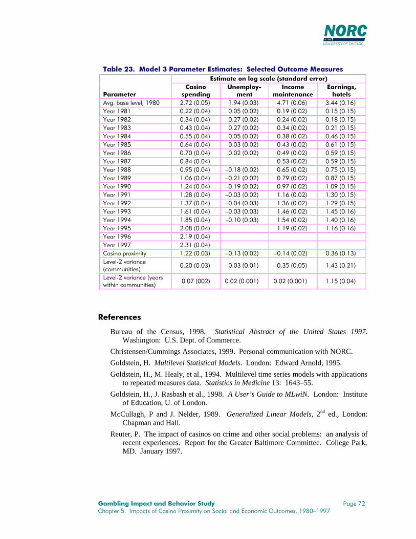
*DPEOLQJ�,PSDFW�DQG�%HKDYLRU�6WXG\ 3DJH���&KDSWHU�����,PSDFWV�RI�&DVLQR�3UR[LPLW\�RQ�6RFLDO�DQG�(FRQRPLF�2XWFRPHV������²����
7DEOH������0RGHO���3DUDPHWHU�(VWLPDWHV���6HOHFWHG�2XWFRPH�0HDVXUHV(VWLPDWH�RQ�ORJ�VFDOH��VWDQGDUG�HUURU�
3DUDPHWHU&DVLQRVSHQGLQJ
8QHPSOR\�PHQW
,QFRPHPDLQWHQDQFH
(DUQLQJV�KRWHOV
$YJ��EDVH�OHYHO������ ����������� ����������� ����������� �����������<HDU����� ����������� ����������� ����������� �����������<HDU����� ����������� ����������� ����������� �����������<HDU����� ����������� ����������� ����������� �����������<HDU����� ����������� ����������� ����������� �����������<HDU����� ����������� ����������� ����������� �����������<HDU����� ����������� ����������� ����������� �����������<HDU����� ����������� ����������� �����������<HDU����� ����������� ²����������� ����������� �����������<HDU����� ����������� ²����������� ����������� �����������<HDU����� ����������� ²����������� ����������� �����������<HDU����� ����������� ²����������� ����������� �����������<HDU����� ����������� ²����������� ����������� �����������<HDU����� ����������� ²����������� ����������� �����������<HDU����� ����������� ²����������� ����������� �����������<HDU����� ����������� ����������� �����������<HDU����� �����������<HDU����� �����������&DVLQR�SUR[LPLW\ ����������� ²����������� ²����������� �����������/HYHO���YDULDQFH�FRPPXQLWLHV�
����������� ����������� ����������� �����������
/HYHO���YDULDQFH��\HDUVZLWKLQ�FRPPXQLWLHV�
���������� ������������ ������������ �����������
5HIHUHQFHV
Bureau of the Census, 1998. Statistical Abstract of the United States 1997.Washington: U.S. Dept. of Commerce.
Christensen/Cummings Associates, 1999. Personal communication with NORC.
Goldstein, H. Multilevel Statistical Models. London: Edward Arnold, 1995.
Goldstein, H., M. Healy, et al., 1994. Multilevel time series models with applicationsto repeated measures data. Statistics in Medicine 13: 1643–55.
Goldstein, H., J. Rasbash et al., 1998. A User’s Guide to MLwiN. London: Instituteof Education, U. of London.
McCullagh, P and J. Nelder, 1989. Generalized Linear Models, 2nd ed., London:Chapman and Hall.
Reuter, P. The impact of casinos on crime and other social problems: an analysis ofrecent experiences. Report for the Greater Baltimore Committee. College Park,MD. January 1997.

*DPEOLQJ�,PSDFW�DQG�%HKDYLRU�6WXG\ 3DJH���&KDSWHU�����&DVH�6WXGLHV�RI�WKH�(IIHFW�RQ�&RPPXQLWLHV�RI�,QFUHDVLQJ�$FFHVV�WR�*DPEOLQJ
&+$37(5�����&$6(�678',(6�2)�7+(�())(&7�21�&20081,7,(6�2),1&5($6,1*�$&&(66�72�0$-25�*$0%/,1*�)$&,/,7,(6
As a part of the NORC team’s work for the Commission, we conducted a 10-communitycase study on the impact of increased access to legalized casino gambling. We randomlyselected our sites from eligible towns and cities across the United States; the onerequirement was that the community have a population of at least 10,000 and lie within a50-mile radius of at least one major casino, as defined by the criterion of at least 500gaming devices, and measuring the distance with commercial place-mapping softwarewith longitude/latitude coordinates. We stratified the selection of cases so that all fourcensus regions of the United States are represented by at least two communities.
Once the communities were selected, we began the process of deciding who theappropriate contacts would be for a telephone interview process. The set of possibilitiesincluded local planners, addiction specialists, social service personnel includingemployment specialists, law enforcement officers, chamber of commerce members, andother persons representing a spectrum of community experience and viewpoints. Wedeveloped a series of open-ended questionnaires that consisted of a core set of questionsplus items that were tailored to each particular type of community member. We thencompiled lists of potential contacts from recommendations of NORC field staff residingin or near these communities, as well as phone directories of government numbers andthe local yellow pages. Finally, in the closing section of each interview, we included anitem asking the respondent whether there was anyone else in the area they wouldrecommend we speak with; this method yielded a number of additional interviews.
Once this process was complete, three experienced interviewers were selected to contactand interview respondents, speaking with seven or eight people in every community.These respondents were often in prominent positions, such as heads of local planningboards and chambers of commerce, chiefs of police, executive directors of mental healthagencies and addiction centers, community development directors, newspaper editors,consumer credit counselors, attorneys, and program directors in local and county socialservice agencies.
We selected our respondents based not only on their positions, but also on the length oftime they have lived in the area and how long they have been in their respective lines ofwork. Many of our respondents have lived in their communities all their lives, and ofthose who have not, many have lived in the area for most of their careers. One interviewhad to be excluded from use due to respondent noncompliance. Our interviews averagedapproximately one-half hour each.
In the sections below, we begin with a brief introduction of the various types of gamingavailable in the case study communities at the current time. We then provide anaggregate overview of the case study sites, discussing common threads we have notedamong the diversity of cities and towns we examined. Finally, we present two of the casestudies in detail. Each case study is an independent, indepth look at how a communityhas responded to legalized casino gaming; taken together, they are a study in contrasts ofthe very different ways that people’s lives can be affected (or not) by the introduction ofcasinos.

*DPEOLQJ�,PSDFW�DQG�%HKDYLRU�6WXG\ 3DJH���&KDSWHU�����&DVH�6WXGLHV�RI�WKH�(IIHFW�RQ�&RPPXQLWLHV�RI�,QFUHDVLQJ�$FFHVV�WR�*DPEOLQJ
7KH�&RPPXQLWLHV
It is important to keep in mind when reading these case studies that people are reporting,more often than not, their own subjective impressions of numbers of people withproblems, of crimes and bankruptcies, and so forth. In many cases, the population of anarea has increased at least modestly (and in some cases dramatically) due to theintroduction of one or more casinos, and in at least two of our case studies, the populationhas increased due to factors that were unrelated to the casinos. What cannot beconcluded based on these vignettes alone is whether the proportion of cases concerning aparticular outcome, negative or positive, has changed.
Where possible, we attempted to verify the descriptions of the types of gamblingavailable in and near the case study communities. With this exception, we shouldemphasize that the information we report here, including the direct and indirect quotesfrom respondents, is based on our interviews alone and have not been validated orinvestigated through external means.
7\SHV�RI�JDPLQJThe sites we chose to examine for our case studies all had a variety of gamblingfacilities
17 within the city limits and nearby; we asked respondents to tell us which
facilities were available within the town proper, as well as any facilities within a 50-mileradius that drew residents. All of these communities were within driving distance of acasino per our selection criteria. Since these casinos are recent additions to the locallandscape, all being introduced within the last 9 years, the issues surrounding theirintroduction were fresh in our respondents’ memories.
Casinos
Until quite recently, casinos were confined to Nevada and Atlantic City. However, in thelast decade, casino gambling has spread to towns and cities across the country, partly inresponse to the need for additional revenues for local and state governments, and partlyas a result of the Indian Gaming Regulatory Act of 1988. The earliest efforts to legalizecasinos outside of Nevada and Atlantic City came in South Dakota and Colorado, wheresmall-stakes casino gambling for the purpose of historic preservation was approved byreferendum in several old mining towns. Published research has reported that the impacton these towns has been enormous, with skyrocketing property values, conversion ofmany businesses to casinos, increased traffic, and increased crime (Long, Clark & Liston1994, in Cox et al. 1997).
17 According to the Commission’s directives, we define the term “gambling” as “an activity that involves
staking or risking something of value upon the outcome of a contest, sporting event, or game of chance, withthe understanding that one may receive something of value in the event of a certain outcome” (RFP, p. 7).Hence, we interpret a “gambling facility” to be any structure where such activity takes place. For thepurposes of this study, we do not include bona fide business transactions governed by the securities laws forthe purchase or sale of stocks, bonds, or securities.

*DPEOLQJ�,PSDFW�DQG�%HKDYLRU�6WXG\ 3DJH���&KDSWHU�����&DVH�6WXGLHV�RI�WKH�(IIHFW�RQ�&RPPXQLWLHV�RI�,QFUHDVLQJ�$FFHVV�WR�*DPEOLQJ
Riverboat casinos in particular have also spread rapidly in the 1990s, and at least one ofour communities is in proximity to one or more riverboats.
18 The first riverboats,
legalized in Iowa in 1991, placed strict limits on both wagers and losses. As riverboatcasinos were legalized in other states, including Illinois, Indiana, Louisiana, Mississippi,and Missouri, these limits were lifted. While these casinos must be located on facilitiesthat look like boats, few of the riverboats actually leave shore. In Mississippi, as well asin Iowa where the earlier restrictions have been eliminated, the term “dockside gambling”is a more accurate description than “riverboat gambling” (Cox et al. 1997), since theminimum requirement is that the gambling occur above a body of water, which may pre-exist or be dredged for the purpose.
The Indian Gaming Regulatory Act created a regulatory structure for gambling on NativeAmerican lands throughout the United States. By establishing a framework fornegotiation between the sovereign tribes and state governments, Congress opened thedoor for Native American tribes to establish casino-style gambling in any state wherecharitable or social gambling is permitted (Eadington 1991). In 1996, more than 700privately owned or Native American casinos were operating in 28 states (InternationalGaming & Wagering Business 1997). At least 3 of our 10 case study sites are based nearone or more tribally owned casinos.
Lotteries
States across the nation have been implementing lotteries since the mid-1960s to fundgovernment services. Today, 37 states have legalized lotteries, and we found state and/ormulti-state lottery games to be present in each of our communities with the exception ofone. With cutbacks in federal spending, pressures on state lotteries to provide revenuesfor government programs have increased. State lotteries now offer a multitude of gamesthat blur the boundaries between their traditional products and other types of gambling,including instant or scratch tickets, daily numbers games, and electronic gaming devicesoffering keno, poker, and line games similar to slot machines at casinos (Cox et al. 1997).In only one of our case study communities did the lottery seem to be a problem for asignificant proportion of residents.
Pari-mutuel gaming
In contrast to lotteries and casinos, the pari-mutuel industry has undergone a dramaticstruggle to stay competitive in the last 10 years. We found a strong representation ofpari-mutuel gaming in our case study sites, with two communities reporting jai alaifrontons in the area, and seven reporting one or more dog and/or horsetracks. However, afull six of the sites reported that one or more tracks have moved or gone bankrupt due tothe increased competition from the casinos. In response, racetracks have sought relieffrom taxation from state legislatures and have also sought to expand their activities.Initially racetracks worked to increase access to their traditional product by establishingoff-track betting systems and broadcasting races from other tracks at their own facilities.More recently, racetracks have sought to compete by offering other types of gambling. In
18 To ensure the confidentiality of our informants, we have tried wherever possible to eliminate information
that could readily identify an individual community. We found in the course of analyzing results from thesesites that the type of casino, particularly whether it was water- or land-based, did not appear to have anydifferential impact on the communities. Therefore, we do not identify riverboats as such in our profiles.

*DPEOLQJ�,PSDFW�DQG�%HKDYLRU�6WXG\ 3DJH���&KDSWHU�����&DVH�6WXGLHV�RI�WKH�(IIHFW�RQ�&RPPXQLWLHV�RI�,QFUHDVLQJ�$FFHVV�WR�*DPEOLQJ
California, several racetracks now have cardrooms where patrons may wager on pokerand other games. In Delaware, Iowa, Rhode Island, and West Virginia, racetracks havebeen permitted to add electronic gaming machines to their traditional products, often withexcellent results for their bottom line (Cox, Lesieur, Rosenthal, & Volberg 1997).Respondents in two of our case study communities reported local referenda on this issue.
Video gaming devices
The innovation widely thought to have the greatest impact in recent years has been theelectronic gaming device, specifically video lottery terminals (VLTs) and video poker.Widely publicized incendiary remarks by one clinician who called video gaming the“crack cocaine” of gambling (Bulkeley 1992), and observations by helpline counselorswho report increased calls from video poker players, indicate the potential value ofundertaking systematic studies of this form of gambling. There are now at least 21 stateswhere electronic gaming devices such as slot machines or video lottery terminals areavailable (McQueen 1996). Of our 10 case study communities, respondents in 5 reportedvideo gaming devices operating (legally and illegally) in local small businesses. Norespondent mentioned this type of game to be particularly addictive or harmful; however,respondents in five communities specifically opined that casinos—in which video gamingdevices are the predominant form of gaming—generate more problems for gamblers thanother types such as the lottery or racetracks.
Other types of games
In addition to these games, all but one community reported bingo. All of these sites hadcharitable bingo, and some also had commercial bingo. In addition, three communitieswere reported to have bookmaking, and one community each was said to have a sportsbar, a bar with a pull-tab dispenser, and keno.
One of the interesting if unexpected outcomes of our interviews was that when we askedrespondents about the effects legalized gaming has had on their communities,respondents seemed to forget all the other kinds of gaming in town and just speak to thecasinos. This is understandable if a community has no other gaming except charitable,which many people do not perceive as really “gambling” but, rather, giving money to agood cause. However, communities reported to have, on average, five major game types.One possible explanation for this focus on casinos may be simple timing. In other words,since, according to our respondents, bingo parlors, lotteries, and tracks have typicallybeen operating in their communities for at least 15 years, it seems reasonable that thesetypes of games have become more a part of day-to-day reality, and that fewer people visitthese types of facilities today, as in the case of racetracks and bingo.
(FRQRPLF�RXWFRPHVA variety of economic themes came through in our case studies; some reflected positivelyon casinos and gaming as a whole, while others did not. The silver linings and darkclouds seemed inextricable from each other. For example, a recurrent positive theme wasthe new employment opportunities that casinos create for local people. In fivecommunities this was cited as a very positive advantage (all but one of these communitieswas located within 10 miles of a major casino). Respondents in the other fourcommunities indicated that unemployment remained a problem, despite former hopes tothe contrary. In two of these sites, as well as in four that cited more jobs, residents

*DPEOLQJ�,PSDFW�DQG�%HKDYLRU�6WXG\ 3DJH���&KDSWHU�����&DVH�6WXGLHV�RI�WKH�(IIHFW�RQ�&RPPXQLWLHV�RI�,QFUHDVLQJ�$FFHVV�WR�*DPEOLQJ
complained that the casinos for the most part provide low-paying and/or part-timepositions with no benefits (four of these communities were located within 10 miles of amajor casino, and two, between 20 and 40 miles of a major casino). One respondentindicated that because of the part-time nature of most of the jobs available in his town,the welfare rolls had not decreased, even though some families had found work in thecasinos. He stated that the reason for this is that people are afraid to take jobs withoutbenefits; while on welfare, they have some assurance that if something happens tothemselves or one of their family members, their medical bills would still be paid.Similarly, in another community, a respondent reported that the welfare rolls havedecreased, but not due to the casinos, because they only brought part-time jobs. On theother hand, one respondent did indicate very clearly that welfare rolls have decreased duein part to the opening of casinos.
19
In addition to casino operations as such, there was growth in the hotel and motel industry(three communities), as well as more funds flowing either directly or indirectly from thecasinos into local government (six communities) and into charitable organizations (threecommunities). Respondents in five communities indicated an increase in construction,and four of these mentioned housing construction in particular. Two communities werereported to have had property values increase. In communities where casinos were builtwithin the city limits, one of the most common concerns was the burden on publicinfrastructure. One town was able to use increased revenues from casinos to upgrade itswater and sewage systems; four reported that either road improvements were needed orthat such improvements had taken place but more work needed to be done. In sixcommunities, at least one resident complained about the increased traffic brought by thecasinos. Three communities reported a growth in the number of retail establishments, buttwo reported a decline since the casinos were built, with a variety of places going out ofbusiness.
All but one of the communities reported an increase in debt problems and/orbankruptcies. One possible explanation that is likely at least in part for this, as told to usin most of these communities, is that people are gambling on their credit cards and takingout cash advances at ATMs in or near the casinos. However, it is also true according to afew of our respondents that because new casinos promise jobs and financial stability fordisadvantaged persons or families, many people move to these towns with their existingdebt problems to try for a better life. If the only work they find available is part-timeservice positions, this may lead to further financial distress and eventually, in severecases, bankruptcy. Respondents in five communities, all but one of which had casinoswithin the town limits, noted that one of the primary problems in the community was thelarge number of working poor. Three communities also mentioned problems withhomelessness, and about four mentioned problems with low-income housing or housingstock.
19 The vast majority of U.S. communities located within 50 miles of a major casino are not located near a
casino with unionized workers, as most unionized casino employees work in the relatively larger, destination-style/resort casinos located in Nevada and Atlantic City. However, due to the concentration and size of thesecasinos, their workers comprise a fair percentage of the total number of casino workers. The sample of casestudies would have to be larger and selected to reflect union presence (for example, 10 communities with and10 without unionized casinos) to permit comparison of the differential effects (if any) that unionization wouldhave on the type of jobs available and related economic effects.
*DPEOLQJ�,PSDFW�DQG�%HKDYLRU�6WXG\ 3DJH���&KDSWHU�����&DVH�6WXGLHV�RI�WKH�(IIHFW�RQ�&RPPXQLWLHV�RI�,QFUHDVLQJ�$FFHVV�WR�*DPEOLQJ
2WKHU�VRFLDO�EHQHILWV�DQG�FRVWVTwo communities reported an overall reduction in crime in their communities, and threereported an overall increase. Interestingly, the youth in particular appear to be havingproblems; five communities reported increases in youth crime, one specific to illegalgambling, and one including illegal gambling. Two of these communities were amongthe three reporting an overall increase in crime, and one was a community reporting anoverall decrease in crime. Illegal gambling did not seem to be much of an issue in thecommunities we looked at; two reported a decrease and one reported an increase, with theremainder either not knowledgeable or not aware of any change having taken place. So-called white collar crimes such as forgery and credit card theft were reported to be on therise in seven of nine communities, including the two towns that reported an overalldecrease in crime; some respondents attributed this change to increased gambling in thecasinos, citing the timing of the increase or the circumstances given in particular newsreports they had seen.
Domestic violence also appeared to be a theme, with respondents in six communitiestelling us they have seen increases in this behavior. Respondents reported, on the whole,no increase in child abuse in their communities. However, six communities had one ormore respondents who said they had seen increases in child neglect, and attributed thisincrease at least in part to parents leaving their children alone at home or in casinolobbies and parking lots while they went to gamble.
A number of social service staff across several communities mentioned they have seen anoverall increase in “family stress” due to gambling. In one community, a mental healthspecialist attributed a recent increase in divorces to casino gambling. Seven communitiesreported either an increase in suicide since the casinos opened, or having seen caseswhere people ended their lives due to problems stemming from their gambling. Inaddition to the need for more gambling treatment, residents of four communities told ofan increased need for general mental health services for gamblers and their families.
Respondents in four communities noted concern over the increased numbers of older andretired persons gambling in the casinos, and respondents in two communities noted anincrease in youth gambling. (As noted in Section 1, data from the national survey do notindicate that particularly large numbers of young adults or elderly are gambling; in fact,past-year gambling statistics for persons between the ages of 18 and 24 and 65 and oldershow that these two groups gamble disproportionately less than one would expect, giventheir proportion of the adult population. See Section 4 for a discussion of gamblingamong 16- and 17-year-olds.)
3UREOHP�JDPEOLQJIn seven of the nine communities we investigated, respondents told us they have seen anincrease in the number of people who are problem and pathological gamblers. Asidefrom the fact that simply more people are gambling, one interviewee pointed out thatonce a community builds a casino, the area may become more attractive to persons whohave the potential to develop into problem gamblers. Furthermore, as the casinos are stilla relative novelty in the communities we investigated, it may be that in time, the numbersof people who find themselves having difficulty controlling their gambling behavior willlearn ways to keep their behavior in check, or will simply lose interest when anothernovel and exciting activity comes along.

*DPEOLQJ�,PSDFW�DQG�%HKDYLRU�6WXG\ 3DJH���&KDSWHU�����&DVH�6WXGLHV�RI�WKH�(IIHFW�RQ�&RPPXQLWLHV�RI�,QFUHDVLQJ�$FFHVV�WR�*DPEOLQJ
While the national prevalence data from the 1998 survey versus its 1975 counterpartindicate an increase in lifetime gambling in the United States, the data do not indicate anincrease in the proportion of people who have gambled in the past year. Therefore, mostof the increase in gambling appears to be from increased activity among those in thepopulation who gamble regularly. From the perspective of our interviewees in at leastfour communities, casino gambling is more habitual than previously available gamingopportunities, so those who gamble do so more frequently and intensively. In fact, it isclear that casinos are “more popular” than other forms of legal gambling in that people, as agroup, spend much more money at them than on other games, other things being equal.People who live within 10 miles of a casino typically spend $400–600 per adult per year oncasino gambling, versus $50–100 per adult per year on state lotteries (in states that havethem) and $10–30 per year on horse and/or greyhound racing (if they live within 10 miles ofa track).
Finally, a major theme that came through in every single case study is that substanceabuse is a major problem in these communities. Respondents complained about the highproportion of drug-related crime, arrests for public intoxication and DWI, youth drug use,and addiction in general. Many interviewees also drew a connection between substanceabuse and gambling, noting that a high proportion of people with one problem will alsohave the other. It is plausible that casinos are affecting substance-using behavior and/orthe reverse. It should also be kept in mind that some of the changes reported in thecommunities may potentially be due to substance abuse.
3XEOLF�RSLQLRQ�UHJDUGLQJ�JDPEOLQJ
One community was strongly in favor of legalized gambling, six indicated a slight bias infavor or a general acceptance of the casinos, two communities were very mixed, and onewas clearly negative. Despite a sample size of only 10 communities, these results arereasonably consistent with how the general population characterizes gambling.
&DVH�6WXG\�2QH���)ORULVVDQW��
The case study interviews were organized in sections, and for the most part, we found itsensible to retain this organization when writing up our findings. We structure each casestudy in the following way: First, we discuss the backgrounds of the interviewees whoparticipated in our survey. Second, we present a summary of the types of gaming that areavailable to residents both within the community itself, as well as nearby, meaning withina 50-mile radius of the city or town. Third, we present our findings on the types ofchanges that have occurred in the community in the past 10 years. Although we stressedto respondents that this question referred to general changes and not just those due togaming, most often respondents told us about the latter; we make this difference explicitwhere needed in the text. Next interviewees were asked what they currently saw as themost important socioeconomic issue in their community. Finally, we asked respondentswhat their views were on how the community generally feels about having legalizedgaming readily available.
20 This name and all other proper names in these case studies are fictitious.

*DPEOLQJ�,PSDFW�DQG�%HKDYLRU�6WXG\ 3DJH���&KDSWHU�����&DVH�6WXGLHV�RI�WKH�(IIHFW�RQ�&RPPXQLWLHV�RI�,QFUHDVLQJ�$FFHVV�WR�*DPEOLQJ
Below we present two of our case studies, chosen in part for the very different impactsgambling has had on these two communities. In Appendix C, we repeat this section, andinclude full discussion of the remaining eight case studies.
2XU�UHVSRQGHQWVFor our case study of the Florissant community, we interviewed a detective in theFlorissant police department, the director of a nonprofit organization specializing in childabuse prevention, an addiction counselor, a city planner, the manager of a consumercredit counseling agency, a tourism office commissioner, and the editor of a localnewspaper. Our respondents have been in their line of work for an average of 15 years(ranging from about 7 years to more than 25). All have lived in the Florissant area ornearby for at least 10 years.
*DPLQJ�LQ�)ORULVVDQWWhen people talk about gaming in Florissant, they are usually talking about casinos.Bingo games are run by nonprofits such as the War Veterans Association, so it appearsthat people view bingo more as making a charitable contribution than as actual gambling.We asked four respondents if they had noticed any trends that appeared to be influencedby the opening or closing of gaming facilities, or by the availability of certain kinds ofgames, and three of them told us that comparisons could not be made, since “We reallyonly have one type.”
Around 1990, state residents voted to allow casino gambling, and within Florissant, thefirst casino opened its doors within a year of the vote. Residents also travel more to anearby state to play in the casinos there. Residents reported some turnover of casinos inthe area, with some of the initial, smaller operations leaving or being bought out by largerfirms. In recent years, several casinos near but not within Florissant have closed or gonebankrupt and changed owners. The two original casinos within the city limits are theonly casinos still operating there and no others have opened and closed in town in themeantime; however, a new casino/hotel complex is expected to open soon.
&RPPXQLW\�FKDQJHVThis city is one of the largest in the state; the opening of the casinos has turned what wasonce a “ghost town” into a popular tourist destination. “[Gambling] is part of thecommunity. Gambling is an active part, it has been involved with community activities.The casinos in [town] are corporate citizens.” In this vein, another stated, “The reasonwe brought [gaming] in was to use it as a leverage point to bring in other business.Gaming is certainly different than most expect it, but the casinos are run by Fortune 500companies, not by gangster types.” In the midst of these changes, the city has beenstriving to maintain a “clean” image. One interviewee reported that “[a] strip jointopened up in downtown [Florissant], but the city took them to court and they left town.”
We asked individuals what community changes they have seen over the last 10 years andwhether they thought any of these changes was related to gaming. Everyone mentionedthe population boom or some change that was related to the increased number of peoplemoving to the area, such as the lack of housing or the traffic and demand for new roads.The thriving economy appears to be the main reason for this influx. People without jobsor many resources come to the Florissant area to start a new life.

*DPEOLQJ�,PSDFW�DQG�%HKDYLRU�6WXG\ 3DJH���&KDSWHU�����&DVH�6WXGLHV�RI�WKH�(IIHFW�RQ�&RPPXQLWLHV�RI�,QFUHDVLQJ�$FFHVV�WR�*DPEOLQJ
Due to the casinos, according to one interviewee, “Investment into schools and publicservices has been greater. Also, there has been more investment in highways andsanitation services.... More people are working; there are more two-income families thanever before. The MSA now has more businesses than any other region . . .”
Gaming, according to the newspaper editor we interviewed, comprises one-quarter toone-half of the local economy, and all respondents except one indicated that they werepleased with the overall direction of the local economy (the exception abstained). Thethread that connects most of these comments is the dramatic improvement in employmentopportunities. Since so many people mentioned this, we break out their comments below.
• According to one respondent who is involved in transportation planning, “We’ve hadto build roads faster, increase housing stock, service businesses.... About 60 percentof these changes are due to gaming.”
• A credit counselor stated, “We see mostly people who have been out of work in otherareas moving here, then paying off creditors....”
• A staff member on the tourist commission stated, “We’ve had significant increases inemployment. We have more two-income households, with more spending power.There’s been a [substantial] rise in per capita income since 1990. It’s generated apositive image about the area, and has attracted other sectors. The timing [of thecasinos being built] was very good.... It has impacted a large portion of the economy,… but not all of it. [New kinds of businesses] have appeared, [and] themanufacturing sector … has strengthened due to independent world conditions. [Thecasinos have] increased exposure for tourism-related business, which we’ve seen indata from [two local associations].
• According to another, “We’ve had a huge increase in employment and tax revenues.It’s a tight labor market, so salaries are increasing. People are moving to Florissantfrom all over the country.”
• A newspaper editor stated that the lower end jobs in the area now have benefits,where before they did not.
• Another respondent stated, “The region’s population has grown [by more than half]in the past 10 years. We have more service-oriented jobs now.”
Respondents also mentioned what could be considered less desirable changes attributableto the casinos, including the rise in problem gambling. According to a respondent in lawenforcement, “there are now Gamblers’ Anonymous meetings in [Florissant] every singlenight of the week, when there used to be none.” An addiction counselor stated thatproblem gamblers were not known before the casinos. The detective stated, “We alreadyhad alcohol and drug addiction services. The casinos opened up . . . and we saw our firstproblem gamblers [within 18 months]. These people were often both alcoholics andproblem gamblers. They have free booze” in the casinos. Two respondents mentionedan increase in bankruptcies. But help is advertised—”They have help-lines now, andmore people are aware that help is available.” Another told us, “Casinos are proactive incombating gambling problems and are bringing money into the community.”
An interviewee in social services mentioned seeing an increase in neglect, though notabuse, over the past several years; “We’ve seen children left unattended, people losing

*DPEOLQJ�,PSDFW�DQG�%HKDYLRU�6WXG\ 3DJH���&KDSWHU�����&DVH�6WXGLHV�RI�WKH�(IIHFW�RQ�&RPPXQLWLHV�RI�,QFUHDVLQJ�$FFHVV�WR�*DPEOLQJ
their money who can’t afford to pay for their food and rent....” Another reported that“[h]ousing prices have gone up. We have traffic congestion and crowded schools.There’s been a strain on infrastructure, construction is up. Not a huge rise in crime.Some traditional neighborhoods have been stressed by growth—high-rise condos,shopping centers, hotels appearing. All of [this change was due to gambling], thoughsome of it was indirect.” One person indicated that chain restaurants were moving in and“chasing away the local restaurants.” A respondent summed up the two sides this way:
It’s been both good and bad. Construction is booming, but there are complaintsof illegal immigrants. The schools have more money, but there’s also theincrease in Gamblers’ Anonymous groups and bankruptcies. Property valueshave gone up, but renters have been hurt, especially seniors. Average rent hasgone from $200 a month to $700a month.
We asked our informants whether they thought the nature or number of crimes inFlorissant had changed. Everyone mentioned an increase in robberies. According to anofficer in law enforcement, crime in general has increased. He added that burglariesaccount for the greatest proportion of crime in the city. Furthermore,
Robberies are up, and there has been a rash of bank robberies … that appear tohave been gambling related. Attempted suicides have also gone up. We havehad some illegal gambling activity in the area. There has also been a rise inprostitution…. The casinos give away alcohol for free, and we have seen a bigrise in alcohol-related crimes. The casinos try to self-regulate, but they areineffective. In Vegas, people catch cabs, but in [Florissant], drunk driving is anissue.
On the other hand, according to a newspaper reporter, prostitution is now less visible thanit was before the casinos, and it should be noted that we were unable to find any escortagencies in the Florissant Yellow Pages. The reporter also stated that “there have beensome isolated, weird crimes, from people freaking out after losing their money. Onewoman faked her own kidnapping, then disappeared for a month.”
&XUUHQW�FRPPXQLW\�LVVXHV
We asked respondents what they thought was the primary social or economic problemtheir community was facing right now, and whether they thought gambling had helpedthe community to control this problem. One respondent was not sure, and did notelaborate. Another interviewee, in social services, had only good things to say:“Economically, we’re doing much better, unemployment is extremely low. Socially, Idon’t know what the primary problem would be.” A respondent on the tourist boardcomplained about the transportation congestion and workforce availability, but added,“Gaming is the cause but also employs [thousands] directly. Tax rates have actually gonedown as we have … extra capital there now.” Similarly, the planner stated, “The cost ofhousing is increasingly too rapidly, but gaming has increased salaries, too.”
The law enforcement interviewee was less positive and pointed to an array of problemshe felt had all been created by the opening of casinos:
Pawnshops are now all over the place operating 24 hours a day, and they don’tworry about dealing in stolen merchandise. There are even places that will letyou sign over the title to your car. We’ve seen some organized crime. We had a
*DPEOLQJ�,PSDFW�DQG�%HKDYLRU�6WXG\ 3DJH���&KDSWHU�����&DVH�6WXGLHV�RI�WKH�(IIHFW�RQ�&RPPXQLWLHV�RI�,QFUHDVLQJ�$FFHVV�WR�*DPEOLQJ
… [situation] where the FBI came in and arrested people.... Casinos are very-image conscious. If there are rapes in the parking lot, the casinos ask us not toreport them. Casinos don’t go after problem gamblers unless they exhibit signsof substance abuse. Also, the increases in bankruptcy.
According to the addiction counselor, the primary problem is Florissant is “[d] rug abuse.Crack has been around 10 or 15 years, and hit a high in the last 4 years.” He added thatgambling does not appear to be related to the drug problem in Florissant. Finally, thenewspaper editor stated that the primary problem Florissant faces is “uncontrolledgrowth. And gambling’s causing it!”
3XEOLF�YLHZV�RQ�JDPLQJ
Next we tried to get a feel for the climate in the community regarding gaming. Peopledid not seem to differ much on their perception that the community felt positively towardthe casinos, although some emphasized the fact that a minority exist who do not approve.Since the community voted to allow casino gaming, it is not surprising that mostinterviewees told us that the majority supports it. However, a few either expounded onthis or disagreed; we include their responses below.
• “There’s no middle of the road. The community is divided. The town votedgambling down before it passed. [Florissant] is a casino town now.”
• “For the most part, it’s understood to be an industry, albeit a recreation/leisureindustry. It’s seen to be positive for our economy.”
• “We had a vote, and it passed. It would depend on whom you talk to. It offends thereligious beliefs of some, but the economic benefits have been significant.”
We also asked people what their expectations had been for when the casinos opened—whether they thought that the community would change in any way. Only one personmentioned having no expectations beforehand. Three people mentioned they believedthat the casinos would bring more tourism to the general area, and two stated that theresult far exceeded their expectations. The flip side to this was expressed by anotherrespondent, who stated, “My expectations were that gaming would cannibalize the area.And it’s happened.” Another stated he had thought that the casinos “would contributemore to treatment programs for compulsive gambling and drug addiction on the local andstate level, though [one casino] did contribute to an awareness program.” Finally, arespondent stated, “I expected a lot more crime and a lot more traffic. Traffic hasincreased, crime has not really increased as much as I expected.”
When it came to their own views on the impact the casinos have had, respondents eitherreiterated their feelings that they have been positive for a majority of the community orwere even more glowing with their praise. In the words of one, “It’s been very good.Very positive. It’s like having Disney World move to your community.”

*DPEOLQJ�,PSDFW�DQG�%HKDYLRU�6WXG\ 3DJH���&KDSWHU�����&DVH�6WXGLHV�RI�WKH�(IIHFW�RQ�&RPPXQLWLHV�RI�,QFUHDVLQJ�$FFHVV�WR�*DPEOLQJ
&DVH�6WXG\�7ZR���+DQVHQ
2XU�UHVSRQGHQWV
For this case study, we interviewed the local chief of police, a mental health programadministrator in the local department of social services, a psychotherapist, a director of acouncil on problem gambling, the local director of community development, a programdirector at a consumer credit counseling service, an administrator in the local chamber ofcommerce, and a reporter for a local newspaper. On the whole, respondents have lived inthe general area for a significant amount of time; with the exception of one respondent(the administrator in the chamber of commerce, who has lived there for just over 5 years);interviewees have lived in the vicinity for a minimum of 20 years.
*DPLQJ�LQ�+DQVHQWe asked respondents about the kinds of gambling available in their area. We found itsignificant that we received such an inconsistent set of responses, and we repeat thembelow:
• “We have lottery games at the gas stations. None, otherwise.”
• “There are three popular bingo halls.”
• “Every kind you can imagine, from legal to illegal.... Charity gaming, illegal sportsbooks, illegal video poker machines in bars.”
• “Zero.”
• “The state lottery.”
• “Absolutely none. [Hansen] was started to be a religious community. It is still dry,and originally no doctors were even allowed.”
• “None that I am aware of, outside of the lottery.”
Respondents also told us about locations outside the immediate community, but within a50-mile radius, that attract local residents. These include a handful of casinos all closeby, which opened around 1990; “numerous bingo halls,” including a tribally ownedparlor; and a dog track. According to one respondent, the dog track has been operatingfor more than a generation. One interviewee stated that the municipal governmentsponsors casino junkets for local senior citizens to a casino about an hour or so fromtown, but he did not know how popular these excursions were.
When asked if any facilities have closed, the majority of the respondents mentioned ahorse track that was a short drive from town; one interviewee added that after the trackclosed, a more local OTB parlor closed. Another respondent stated, “None [have closed],because there haven’t been any.”
The respondents in this case study were unique in that they interpreted our use of thephrase “legalized gambling” with the understanding that this category includes a varietyof types of games. In every other community in which we conducted interviews,respondents appeared to equate “legalized gambling” with casino gaming. In thisparticular town, one interviewee told us that people tend to spend more money at bingo

*DPEOLQJ�,PSDFW�DQG�%HKDYLRU�6WXG\ 3DJH���&KDSWHU�����&DVH�6WXGLHV�RI�WKH�(IIHFW�RQ�&RPPXQLWLHV�RI�,QFUHDVLQJ�$FFHVV�WR�*DPEOLQJ
halls than at the casinos, but added that the share taken by casinos is growing. Anotherrespondent commented that she has seen people in town spending “a disproportionateamount of their meager incomes” on lottery tickets, partly because it is “just soconvenient to play.” A credit counselor told us that about one-half of the people sheworks with play the lottery regularly, and guessed that they spend about ten dollars perweek on tickets. Another resident commented on the popularity of the lottery as well,adding “We occasionally see thefts of lottery tickets from convenience stores, or adomestic dispute over a winning lottery ticket.”
&RPPXQLW\�FKDQJHVHansen is small town that has recently experienced some economic troubles. Severalrespondents told us that a particularly large plant recently closed in the area, whichaffected the tax base significantly. According to an administrator in the local chamber ofcommerce, this shutdown “had a major impact on our community. [Hundreds of] jobswere lost.” However, the newspaper reporter indicated that most of the plant’semployees were from out of town. The real impact seems to have been in revenue loss;three respondents told us that this shutdown has impacted as much as half of the tax base.The chief of police added that the schools have been particularly hard hit.
The director of community development defined the town as a “low-to-moderate incomecommunity, primarily residential in nature. Like many older, inner-suburbancommunities, we are struggling to provide services, meet demands.” Another issue thetown is trying to handle is that people are moving out to newer suburbs. “We face a lackof local jobs, and our taxes are based on residential property.” Another respondent toldus that the town has a high percentage of rental housing per capita, and that they aretrying to take advantage of a local housing boom in the county to improve the housingsituation.
We asked respondents if they personally were pleased with the overall direction of theireconomy at this point. Two respondents indicated they were, while four respondentsindicated dissatisfaction, including
• One interviewee who cited the recent closing of a large plant;
• A program administrator in mental health, who told us that “medical services areoutrageous in our community. If they’re going to legalize gambling, they should putmoney into treatment, across all areas”;
• The director of community development, who stated the community needs “a broadereconomic base, more industrial and business development in the community”; and
• A newspaper reporter, who commented that “[Hansen] really needs to wean itself offof the tax money [from the power plant].”
One respondent declined to answer.
The director of community development told us, “We are part of [a] metro region, andare influenced by [the city]…. We constantly face movement to the green fields, newsuburbs. Urban sprawl contributes to our problems and is part of our planning process.We face a lack of local jobs, and our taxes are based on residential property.” Aside fromthe plant closing, however, “The community has not changed much since 1990.... We

*DPEOLQJ�,PSDFW�DQG�%HKDYLRU�6WXG\ 3DJH���&KDSWHU�����&DVH�6WXGLHV�RI�WKH�(IIHFW�RQ�&RPPXQLWLHV�RI�,QFUHDVLQJ�$FFHVV�WR�*DPEOLQJ
have an ongoing economic development program, though. We have no specific sectorstargeted, but would like to attract light manufacturing jobs. We’re too far from theinterstate to attract warehouse and distribution business.”
According to another interviewee, a couple of new restaurants and banks have openedover the past several years, but overall “There’s not a huge commercial base.... Basically,service industries are all that’s moving in.... It tends to be a strictly residentialcommunity.” The credit counselor commented on the job situation, saying, “We havelow unemployment, but they’re all low-paying, service-industry jobs.”
None of our informants indicated that the local gaming establishments have had anyaffect on the local economy, not even on tourist-related businesses. People from out oftown visit the community to go to the park or to walk along the marina, and the town hasan excellent medical center. In the past 2 years, the chamber of commerce representativesaid, only one person has asked her about gambling in the area.
On the other hand, some controversy exists surrounding whether the opening of casinosnearby has had an affect on individuals in the town. The program director for a consumercredit counselor service said that the town has “seen higher and higher credit card debt....The number of individuals filing for both Chapter 7 and Chapter 13 bankruptcies [i.e.,personal bankruptcy] has increased.” She told us she did not see any connection betweenthese trends and gambling, saying, “gambling losses play a minor role in the debtproblems that we are now seeing.” But she added, “Casino gambling has increased in thearea. A few families have come in with gambling problems.” According to a mentalhealth administrator, the town’s relatively high poverty rate has made residents morevulnerable to potentially addictive behaviors. “People think that they can get rich [if theygamble], and the people that we treat tend to be on the lower end of the income scale in[the] county.... The economic impact creates stress, which creates substance abuse andother negative impacts.”
With regard to changes in social services in the community, the mental health programadministrator told us she has seen “extreme changes” in her agency, and the demand foraddiction services far exceeds their resources. Not-for-profit companies in particularhave been suffering. “It’s been a steady increase, maybe there was a surge since the early1990s. The courts have adopted an interventionist approach as opposed to a punitive one.More people are getting court-ordered treatment instead of jail time. [However,] we’relimited in the number of sessions we can provide and the number of people that we cantreat because of financial concerns.”
Since the agency is not set up to deal with gambling addiction, and none of thecounselors are certified gambling counselors, staff only deal with gambling indirectly.The administrator added that no services exist in the immediate area specifically to helppeople with gambling problems, but she said that gambling treatment centers have beenopening in the state. She told us that her agency now refers more people to gamblingtreatment than they used to. “I’m sure there’s an indirect effect with drinking and otherkinds of drug abuse. I think it’s a cumulative effect. Gambling, drinking and drugsincrease domestic violence and poverty. Can I track that as a statistic? No. That’s moremy opinion than anything I could prove.”
The director of the council on problem gambling also spoke to this issue for the state as awhole:

*DPEOLQJ�,PSDFW�DQG�%HKDYLRU�6WXG\ 3DJH���&KDSWHU�����&DVH�6WXGLHV�RI�WKH�(IIHFW�RQ�&RPPXQLWLHV�RI�,QFUHDVLQJ�$FFHVV�WR�*DPEOLQJ
There’s a tremendous need for treatment of gambling problems. There is betterawareness now, people show up stating that they and their families havegambling problems. Taxpayers also spend much more for prosecution andincarceration of compulsive gamblers. This is often not factored into theequation.... We have seen a doubling, at least, in the number of GamblersAnonymous groups in the state ... over the past 5 to 6 years. The need forservices has expanded dramatically.... We’ve trained [hundreds of]professionals in diagnosis, assessment, and treatment over the last 3 to 4 yearsstatewide.
We also asked respondents about ways in which crime and law enforcement may havechanged in their communities over the last decade or so. According to the chief of police,all types of crime are prevalent in this community, and most of it is related to drugs andgangs. In particular, sales of illegal drugs “are way up.” The newspaper reporter told us,“Substance abuse is still a big problem…. Crack-cocaine [for instance], but it’sdeclining. Drug raids have tapered off, but are very severe when they occur. Theimproved economy also helps, though it’s really not better in [Hansen].” The local policedepartment has responded to this problem by becoming more involved in communitypolicing: “The districts haven’t changed, but officers are permanently assigned to areasnow, and we used to rotate them.”
The chief of police faxed us a brief table displaying major offenses (e.g., homicide,burglary, arson) in the town from 1994 to 1997. These data show a downward trend inviolent offenses, and particularly in robberies and property offenses, although it we havenot calculated whether these changes are statistically significant. The chief of police toldus that although specific types of crime have increased, these trends are not connected togambling. In addition, he reported that illegal gambling has not increased since thecasinos have opened, and a program administrator in mental health told us she is notaware of any trends in underage gambling.
When we asked the director of the council on problem gambling whether he thought thatcrime has increased, he did not speak to the Hansen community in particular, but didspeak to the state as a whole:
Certainly. We have noticed a statewide increase in paper crime—forgery, fraud,theft and embezzlement—none of which are classified by law enforcementofficials as gambling-related crime. Criminal activities of compulsive gamblersare often not recorded. The crime question is being asked incorrectly, and theresults could be completely misleading.
The newspaper reporter told us that, overall; crime in the area has gone down. However,he added that “transient residents” are susceptible to gang activity, and that the townmostly has drug-related crime like robberies and vandalism. “I don’t think the policeforce would want gambling in the area. Crime is already somewhat high for acommunity our size.”
Adolescent suicide rates may also be on an upward trend. The mental healthadministrator told us, “I think teenage suicide is up slightly in this community, though Idon’t know what the statistics are county-wide. I’m not aware of any connectionbetween suicide trends and gambling, but I’m not saying that they don’t exist.”

*DPEOLQJ�,PSDFW�DQG�%HKDYLRU�6WXG\ 3DJH���&KDSWHU�����&DVH�6WXGLHV�RI�WKH�(IIHFW�RQ�&RPPXQLWLHV�RI�,QFUHDVLQJ�$FFHVV�WR�*DPEOLQJ
&XUUHQW�FRPPXQLW\�LVVXHVWe asked respondents to tell us what they thought was the primary social or economicproblem their community faces at this time, and whether they believe legalized gamblinghas had any affect on the community’s efforts to control this problem. One intervieweetold us he did not know. Two respondents mentioned drugs, one also mentioning gangs,and the other explicitly including alcohol. The latter respondent stated, “Crack cocaine isfar too accessible, far too cheap. Our treatment of crack-cocaine users is at an all-timehigh. [Legalized gambling] certainly has a negative impact.” Two respondentsmentioned the tax base, one calling it “unstable,” and the other saying “We have a seriouscrisis.” Neither could say that gambling has helped or worsened this problem. Oneinterviewee mentioned the lack of high-paying jobs, adding that she was not aware of anychange in this area due to the opening or closing of gambling facilities. Finally, onerespondent told us he saw the primary problem as “pathological gambling.... Legalizedgambling has brought the problem more to the surface, but at the same time, has notmade it easier to deal with. In [this state], there’s absolutely no state funding to addresscompulsive gambling problems. The casinos also kick in no money for treatmentprograms.”
3XEOLF�YLHZV�RQ�JDPLQJ
Next we asked respondents how they thought the community generally feels about havinglegalized gaming readily available. We found the nature of our responses to depart ratherradically from the kinds of responses we were given in other case study communities.Basically, the respondents in this town were split into two camps: Interviewees who feltthat overall, the community was pleased with having gambling available due to theirbeing uninformed about the negative impacts, and interviewees who felt that the majorityof the community was opposed to gambling for religious reasons. A sampling ofresponses follow:
• “I think they’re ecstatic. They think that more money’s going into education, thatthey won’t have to pay higher taxes. They don’t grasp the negative impact. They areused to segregating off crime and substance abuse in a societal kind of way.”
• “I think most of the community likes it, and it’s based on ignorance. It’s not even thegambling that the community likes, it’s the fantasy of winning.”
• “[Hansen] was originally formed as a religious community. Most residents are notinterested in having gambling.”
• “I’m sure it would fail miserably in this town. They tried to get alcohol on the ballotin the November election, and it failed to pass.”
Next we asked interviewees what their personal expectations were for the effects of anearby gaming establishment on the community before the casinos opened, and whethertheir expectations have been borne out. Most said they did not have expectations, and sohad no surprises when the casinos opened. The two respondents who did haveexpectations expressed them in the following way:
• “My expectations were that it would be a net loss to the community, and they havebeen borne out. I see things that others don’t see. For every winner, there’s a loser.It’s easy to spot fire plugs painted, streets paved, buildings built... [Also, I have been

*DPEOLQJ�,PSDFW�DQG�%HKDYLRU�6WXG\ 3DJH���&KDSWHU�����&DVH�6WXGLHV�RI�WKH�(IIHFW�RQ�&RPPXQLWLHV�RI�,QFUHDVLQJ�$FFHVV�WR�*DPEOLQJ
surprised] that the public would continue to be as blind as they are to the loss side ofthe equation.”
• “I would expect it to be detrimental. In [other communities in the state that haveopened casinos], jobs were created, but the economic runoff that they expected hasnot been realized.”
Finally, we asked the respondents what their overall feelings were about the effectslegalized gambling has had on their communities. We repeat their comments below (tworespondents were not asked this question):
• “It has social and economic negative impacts, and contributes to addiction. I don’tsupport it, personally.”
• “Negative.”
• “I can’t say that there’s any [effects] that I know of.”
• “I’m not aware of any community effects, but gambling can be devastating for anindividual family.”
• “I’ve never even bought a lottery ticket, but don’t see a big problem with gamblingpersonally.... I’m sure there’s an impact, probably slight.”
5HIHUHQFHV
Bulkeley, W. July 14, 1992. “Video Betting, Called ‘Crack of Gambling,’ isSpreading,” The Wall Street Journal B1.
Cox, S., Lesieur, H., Rosenthal, R., and Volberg, R. 1997. Problem andPathological Gambling in America: The National Picture. New York: NationalCouncil on Problem Gambling.
Eadington, W.R. 1991. “Public Policy Considerations and Challenges and theSpread of Commercial Gambling.” In Gambling and Public Policy:International Perspectives. W.R. Eadington and J.A. Cornelius (eds). Reno,NV: University of Nevada Press.
Harrah’s Entertainment, Inc. 1996. Harrah’s Survey of Casino Entertainment.Memphis, TN: Harrah’s Marketing Communications.
Heubusch, K. May 1997. “Taking Chances on Casinos.” American Demographics.http://www.demographics.com/publications/ad/97_ad/9705_ad/ad970530.htm
IGWB (International Gaming & Wagering Business) Online. August 15, 1997.“1996 Gross Annual Wager: Growth in Gaming Industry Slowed Last Year inBoth Handle and Revenue.” http://www.igwb.com/news/gaw.html, accessedFebruary 4, 1998.
McQueen, P.A. 1996. “North American Gaming at a Glance.” InternationalGaming & Wagering Business 17(9): 52–56.
Scripps Howard News Service and Ohio University. “Recent Bush Center ResearchProjects: Gambling.” http://www.scripps.ohiou.edu/research.htm#gamble,accessed February 6, 1998.