Game Theory 2 - Mechanism Design with Transfers

1 Introduction

Consider a seller who owns an indivisible object, say a house, and wants to sell it to a set

of buyers. Each buyer has a value for the object, which is the utility of the house to the

buyer. The seller wants to design a selling procedure, an auction for example, such that he

gets the maximum possible price (revenue) by selling the house. If the seller knew the values

of the buyers, then he would simply offer the house to the buyer with the highest value

and give him a “take-it-or-leave-it” offer at a price equal to that value. Clearly, the (highest

value) buyer has no incentive to reject such an offer. Now, consider a situation where the

seller is unaware of the values of the buyers. What selling procedure will give the seller the

maximum possible revenue? A clear answer is impossible if the seller knows nothing about

the values of the buyer. However, the seller may have some information about the values of

the buyers. For example, the possible range of values, the probability of having these values

etc. Given these information, is it possible to design a selling procedure that guarantees

maximum (expected) revenue to the seller?

In this example, the seller had a particular objective in mind - maximizing revenue. Given

his objective he wanted to design a selling procedure such that when buyers participate in

the selling procedure and try to maximize their own payoffs within the rules of the selling

procedure, the seller will maximize his expected revenue over all such selling procedures.

The study of mechanism design looks at such issues. A planner (mechanism designer)

needs to design a mechanism (a selling procedure in the above example) where strategic

agents can interact. The interactions of agents result in an outcome. While there are

several possible ways to design the rules of the mechanism, the planner has a particular

objective in mind. For example, the objective can be efficiency (maximization of the total

welfare of agents) or maximization of his own surplus (as was the case in the last example).

Depending on the objective, the mechanism needs to be designed in a manner such that when

strategic agents interact, the resulting outcome gives the desired objective. One can think of

mechanism design as the reverse engineering of game theory. In game theory terminology, a

mechanism induces a game whose equilibrium outcome is the objective that the mechanism

designer has set.

1.1 Private Information and Utility Transfers

The main input to a mechanism design problem is the set of possible outcomes or alternatives.

Agents have preferences over the set of alternatives. These preferences are unknown to the

mechanism designer. Mechanism design problems can be classified based on the amount of

information asymmetry present between the agents and the mechanism designer.

1

1. Complete Information: Consider a setting where an accident takes place on the

road. Three parties (agents) are involved in the accident. Everyone knows perfectly

who is at fault, i.e., who is responsible to what extent for the accident. The traffic

police comes to the site but is unaware of the information agents have. The mechanism

design problem is to design an institution where the traffic police’s objective (to punish

the true offenders) can be realized. The example given here falls in a broad class of

problems where agents perfectly know all the information between themselves, but the

mechanism designer does not know this information.

2. Private Information and Interdependence: Consider the sale of a single object.

The utility of an agent for the object is his private information. This utility information

may be known to him completely, but usually not known to other agents and the

mechanism designer. There are instances where the utility information of an agent

may not be perfectly known to him. Consider the case where a seat in a flight is

being sold by a private airlines. An agent who has never flown this airlines does not

completely know his utility for the flight seat. However, there are other agents who

have flown this airlines and have better utility information for the flight seat. So, the

utility of an agent is influenced by the information of other agents. Still the mechanism

designer is not aware of any information agents have.

Besides the type of information asymmetry, mechanism design problems can also be

classified based on whether monetary transfers are involved or not. Transfers are a means to

redistribute utility among agents.

1. Models without transfers. Consider a setting where a set of agents are deciding

to choose a candidate in an election. There is a set of candidates in the election, and

each of them is an alternative. Agents have preference over the candidates. Usually

monetary transfers are not allowed in such voting problems.

2. Models with transfers and quasi-linear utility. The single object auction

is a classic example where monetary transfers are allowed. If an agent buys the object

he is expected to pay an amount to the seller. The net utility of the agent in that

case is his utility for the object minus the payment he has to make. Such net utility

functions are linear in the payment component, and is referred to as the quasi-linear

utility functions.

In this course, we will focus on (a) voting models without transfers and (b) models

with transfers and quasi-linear utility. In voting models, we will mainly deal with or-

dinal preferences, i.e., intensities of preferences will not matter. We will mainly focus on

the case where agents have private information about their preferences over alter-

natives. Note that such private information is completely known to the respective agents

but not known to other agents and the mechanism designer.

2

1.2 Examples in Practice

The theory of mechanism design is probably the most successful story of game theory. Its

practical applications are found in many places. Below, we will look at some of the applica-

tions.

1. Matching. Consider a setting where students need to be matched to schools. Stu-

dents have preferences over schools and schools have preference over students. What

mechanisms must be used to match students to schools? This is a model without any

transfers. Lessons from mechanism design theory has been used to design centralized

matching mechanisms for major US cities like Boston and New York. Such mechanisms

and its variants are also used to match kidney donors to patients, doctors to hospitals,

and many more.

2. Sponsored Search Auction. If you search for a particular keyword on Google, once

the search results are displayed, one sees a list of advertisements on the right of the

search results. Such slots for advertisements are dynamically sold to potential buyers

(advertising companies) as the search takes place. One can think of the slots on a page

of search result as a set of indivisible objects. So, the sale of slots on a page can be

thought of as simultaneous sale of a set of indivisible objects to a set of buyers. This

is a model where buyers make payments to Google. Google uses a variant of a well

studied auction in the auction theory literature. Bulk of Google’s revenues come from

such auctions.

3. Spectrum Auction. Airwave frequencies are important for communication. Tradition-

ally, Govt. uses these airwaves for defense communication. In late 1990s, various

Govts. started selling (auctioning) airwaves for private communication. Airwaves for

different areas were sold simultaneously. For example, India is divided into various

“circles” like Delhi, Punjab, Haryana etc. A communication company can buy the air-

waves for one or more circles. Adjacent circles have synergy effects and distant circles

have substitutes effects on utility. Lessons from auction theory were used to design

auctions for such spectrum sale in US, UK, India, and many other European countries.

The success of some of these auctions have become the biggest advertisement of game

theory.

2 Mechanism Design with Transfers

2.1 A General Model

The set of agents is denoted by N = 1, . . . , n. The set of potential social decisions or

outcomes or alternatives is denoted by the set A, which can be finite or infinite. For our

3

purposes, we will assume A to be finite. Every agent has a private information, called his

type. The type of agent i ∈ N is denoted by ti which lies in some set Ti. I emphasise that ti

can be multi-dimensional - a vector of dimension greater than or equal to 1. I denote a profile

of types as t = (t1, . . . , tn) and the product of type spaces of all agents as T n = ×i∈NTi. The

type space Ti reflects the information the mechanism designer has about agent i.

Agents have preferences over alternatives which depends on their respective types. This

is captured using a utility function. The utility function of agent i ∈ N is vi : A × Ti → R.

Thus, vi(a, ti) denotes the utility of agent i ∈ N for decision a ∈ A when his type is ti ∈ Ti.

Note that the mechanism designer knows Ti and the utility function vi. Of course, he does

not know the realizations of each agent’s type.

We will restrict attention to this setting, called the private values setting, where the

utility function of an agent is independent of the types of other agents, and is completely

known to him. Below are two examples to illustrate the ideas.

A Public Project

Suppose a bridge needs to be built across a river in a city. The residents need to take a

decision whether to build the bridge or not. Hence, A = 0, 1, where 0 indicates that the

bridge is not built and 1 indicates that it is built. There is a total cost c from building the

bridge which the residents share. The value for the bridge for resident i ∈ N is ti ∈ R (his

type). Hence, utility of agent i with type ti when the decision is a ∈ 0, 1 can be written

as vi(a, ti) = a(

ti −cn

)

.

Allocating Multiple Objects

A set of indivisible goods M = 1, . . . , m need to be allocated to a set of agents N =

1, . . . , n. Let Ω = S : S ⊆ M be the set of bundles of goods. The type of an agent i ∈ N

is a multi-dimensional vector ti ∈ R|Ω|+ , where ti(S) indicates the value of agent i ∈ N for a

bundle S ∈ Ω. Here, a decision is an allocation vector x ∈ 0, 1n×|Ω|, where xi(S) ∈ 0, 1

indicates whether bundle S ∈ Ω is allocated to agent i ∈ N . Of course, an allocation x must

satisfy the feasibility constraints:

∑

i∈N

∑

S∈Ω:j∈S

xi(S) ≤ 1 ∀ j ∈ M

∑

S∈Ω

xi(S) ≤ 1 ∀ i ∈ N.

The first constraint says that no good can be allocated to more than one agent. The second

constraint says that if an agent is allocated multiple goods, then it should be treated as a

bundle of goods - hence, every agent can be allocated at most one bundle. Let X be the set

4

of all allocations (satisfying the feasibility constraints). Then A = X. The utility of agent i

when his type is ti and allocation is x ∈ X is given by

vi(x, ti) =∑

S∈Ω

ti(S)xi(S).

2.2 Allocation Rules

A decision rule or an allocation rule f is a mapping f : T n → A. Hence, an allocation

rule gives a decision as a function of the types of the agents. From every type profile matrix,

we construct a valuation matrix with n rows (one row for every agent) and |A| columns. An

entry in this matrix corresponding to type profile t, agent i, and a ∈ A has value vi(a, ti).

We show one valuation matrix for N = 1, 2 and A = a, b, c below.

[

v1(a, t1) v1(b, t1) v1(c, t1)

v2(a, t2) v2(b, t2) v2(c, t2)

]

Here, we give some examples of allocation rules.

• Constant allocation: The constant allocation rule f c allocates some a ∈ A for every

t ∈ T n. In particular, there exists a a ∈ A such that for every t ∈ T we have

f c(t) = a.

• Dictator allocation: The dictator allocation rule fd allocates the best decision of

some dictator agent i ∈ N . In partcular, let i ∈ N be the dictator agent. Then, for

every ti ∈ Ti and every t−i ∈ T−i,

fd(ti, t−i) ∈ arg maxa∈A

vi(a, ti).

It picks a dictator i and always chooses the column in the valuation matrix for which

the i row has the maximum value in the valuation matrix.

• Efficient allocation: The efficient allocation rule f e is the one which maximizes the

sum of values of agents. In particular, for every t ∈ T n,

f e(t) ∈ arg maxa∈A

∑

i∈N

vi(a, ti).

This rule first sums the entries in each of the columns in the valuation matrix and picks

a column which has the maximum sum.

Hence, efficiency implies that the total value of agents is maximized in all states of the

world (i.e., for all possible type profiles of agents).

5

Consider an example where a seller needs to sell an object to a set of buyers. In any

allocation, one buyer gets the object and the others get nothing. The buyer who gets

the object realizes his value for the object, while others realize no utility. Clearly, to

maximize the total value of the buyers, we need to maximize this realized value, which

is done by allocating the object to the buyer with the highest value.

• Anti-efficient allocation: The anti-efficient allocation rule fa is the one which min-

imizes the sum of values of agents. In particular, for every t ∈ T n

fa(t) ∈ arg mina∈A

∑

i∈N

vi(a, ti).

• Weighted efficient allocation: The weighted efficient allocation rule fw is the one

which maximizes the weighted sum of values of agents. In particular, there exists

λ ∈ Rn+ \ 0 such that for every t ∈ T n,

fw(t) ∈ arg maxa∈A

∑

i∈N

λivi(a, ti).

This rule first does a weighted sum of the entries in each of the columns in the valuation

matrix and picks a column which has the maximum weighted sum.

• Affine maximizer allocation: The affine maximizer allocation rule fa is the one

which maximizes the weighted sum of values of agents and a term for every allocation.

In particular, there exists λ ∈ Rn+ \ 0 and κ : A → R such that for every t ∈ T n,

fa(t) ∈ arg maxa∈A

[

∑

i∈N

λivi(a, ti) − κ(a)]

.

This rule first does a weighted sum of the entries in each of the columns in the valuation

matrix and subtracts κ term corresponding to this column, and picks the column which

has this sum highest.

• Max-min (Rawls) allocation: The max-min (Rawls) allocation rule f r picks the

allocation which maximizes the minimum value of agents. In particular for every

t ∈ T ,

f r(t) ∈ arg maxa∈A

mini∈N

vi(a, ti).

This rule finds the minimum entry in each column of the valuation matrix and picks

the column which has the maximum such minimum entry.

6

2.3 Payment Functions

The fact that the decision maker is uncertain about the types of the agents makes room for

agents to manipulate the decisions by misreporting their types. To give agents incentives

against such manipulation, payments are often used. Formally, a payment function (of agent

i) is a mapping pi : T n → R, where pi(t) represents the payment of agent i when type profile

is t ∈ T n. Note that pi(·) can be negative or positive or zero. A positive pi(·) indicates that

the agent is paying money.

In many situations, we want the total payment of agents to be either non-negative (i.e.,

decision maker does not incur a loss) or to be zero. A payment rule p = (p1, . . . , pn) is

feasible if∑

i∈N pi(t) ≥ 0 for all t ∈ T n. Similarly, a payment rule p = (p1, . . . , pn) is

balanced if∑

i∈N pi(t) = 0 for all t ∈ T n.

2.4 Social Choice Functions and Mechanisms

A social choice function is a pair F = (f, p = (p1, . . . , pn)), where f is an allocation rule

and p1, . . . , pn are payment functions of agents. Hence, the input to a social choice function

is the types of the agents. The output is a decision and payments given the reported types.

Figure 1 gives a pictorial description of a social choice function.

-

-

-

-.....................................................................................................................................................................................................................................................................................................................................

-.....................................................................................................................................................................................................................................................................................................................................

-

--

-

-.................................................................................................................................................................................................................................

f(t)

p1(t)p2(t)

pn(t)

t1

t2

tn

Social Choice Function (f, p)

Figure 1: Social Choice Function

Under a social choice function F = (f, p) the utility of agent i ∈ N with type ti when all

agents “report” t as their types is given by

ui(t, ti, F = (f, p)) = vi(f(t), ti) − pi(t).

This is the quasi-linear utility function, where net utility of the agent is linear in his payment.

A mechanism is a pair (M, g), where M = M1 × . . . × Mn is the message spaces of

agents and g is a mapping g : M → A × Rn. The mapping g is called an outcome function.

The message spaces are restrictions on the strategies of agents in a mechanism.

For every profile of messages m = (m1, . . . , mn) ∈ M , the outcome function g(m) =

(ga(m), g1(m), . . . , gn(m)) gives a decision ga(m) ∈ A and a payment gi(m) to every agent

i ∈ N . Hence, a mechanism is more general than a social choice function. In a social choice

function, the input is types of agents (for example, values of bidders in an auction) but in a

7

mechanism it is messages from agents. A message can be anything arbitrary. For example,

in an auction setting it can be a sequence of bounds on the value of a bidder. The output of a

mechanism and a social choice function is the same - an allocation and a vector of payments.

Clearly, a social choice function is also a mechanism where the messages are restricted to be

types only. Figure 2 gives a pictorial description of a mechanism.

-

-

-

-

-

-

XXXXXz

-

*

-

Mechanism (M, g)M2

ga(m)

g1(m)

gn(m)

M1

Mn

mn

m2

m1

g2(m)

Figure 2: Mechanism

A direct mechanism is a mechanism (M, g) where Mi = Ti for all i ∈ N , and g = F =

(f, p) is a social choice function. Hence, every social choice function is a direct mechanism.

2.4.1 Examples of Mechanisms

Let us revisit the auction of single indivisible good example. One possible mechanism is

where buyers are directly asked to report their values (types) and an allocation and payment

is determined, e.g., the buyer with the highest value wins and pays the amount he reported

(first-price auction). This is a direct mechanism.

Another possible mechanism is a price-based mechanism. The auctioneer announces a

low price and asks if any buyer is interested in buying the good at this price. If more than

one agent is interested, the price is raised by a small amount. Else, the only interested buyer

is awarded the object at the current price, and the process is repeated. The messages of a

buyer in this mechanism is a sequence of prices and demands of that buyer at these prices.

As can be seen the second mechanism is considerably more complicated, in terms of

description, than the first one.

3 Dominant Strategy Incentive Compatibility

The goal of mechanism design is to design the message space and outcome function in a way

such that when agents participate in the mechanism they have (best) strategies (messages)

that they can choose as a function of their private types such that the desired outcome is

achieved. The most fundamental, though somewhat demanding, notion in mechanism design

8

is the notion of dominant strategies. A strategy mi ∈ Mi is a dominant strategy at ti ∈ Ti

in a mechanism (M, g) if for every m−i ∈ M−i1 we have

vi(ga(mi, m−i), ti) − gi(mi, m−i) ≥ vi(ga(mi, m−i), ti) − gi(mi, m−i) ∀ mi ∈ Mi.

Notice the strong requirement that mi has to be the best strategy for every strategy profile

of other agents. Such a strong requirement limits the settings where dominant strategies

exist.

A social choice function F = (f, p) is implemented in dominant strategies by a mech-

anism (M, g) if there exists mappings for every agent i ∈ N , mi : Ti → Mi such that mi(ti)

is a dominant strategy at ti for every ti ∈ Ti and ga(m(t)) = f(t) for all t ∈ T n and

gi(m(t)) = pi(t) for all t ∈ T n and for all i ∈ N .

A direct mechanism (or associated social choice function) is strategy-proof if for every

agent i ∈ N and every ti ∈ Ti, ti is a dominant strategy at ti. In other words, (f, p) is

strategy-proof if for every agent i ∈ N , every t−i ∈ T−i, and every si, ti ∈ Ti, we have

vi(f(ti, t−i), ti) − pi(ti, t−i) ≥ vi(f(si, t−i), ti) − pi(si, t−i),

i.e., truth-telling is a dominant strategy.

So, to verify whether a social choice function is implementable or not, we need to search

over infinite number of mechanisms whether any of them implements this SCF. A fundamen-

tal result in mechanism design says that one can restrict attention to the direct mechanisms.

Proposition 1 (Revelation Principle) If a mechanism (M, g) implements a social choice

function F = (f, p) in dominant strategies then the direct mechanism F = (f, p) is strategy-

proof.

Proof : Fix an agent i ∈ N . Consider two types si, ti ∈ Ti. Consider t−i to be the report of

other agents. Let mi(ti) = mi and m−i(t−i) = m−i, where for all j ∈ N , mj is the dominant

strategy message function of agent j ∈ N . Similarly, mi(si) = m′i. Then, using the fact that

(f, p) is implemented by (M, g) in dominant strategies, we get

vi(f(ti, t−i), ti) − pi(ti, t−i) = vi(ga(mi, m−i), ti) − gi(mi, m−i)

≥ vi(ga(m′i, m−i), ti) − gi(m

′i, m−i)

= vi(f(si, t−i), ti) − pi(si, t−i).

Hence, (f, p) is strategy-proof.

Thus, a social choice function F = (f, p) is implementable in dominant strategies if

and only if the direct mechanism (f, p) is strategy-proof. Revelation principle is a central

1 Here, m−i is the profile of messages of agents except agent i and M

−i is the cross product of message

spaces of agents except agent i.

9

result in mechanism design. One of its implications is that if we wish to find out what

social choice functions can be implemented in dominant strategies, we can restrict attention

to direct mechanisms. This is because, if some non-direct mechanism implements a social

choice function in dominant strategies, revelation principle says that the corresponding direct

mechanism is also strategy-proof. Also, note that the payments in any mechanism which

implements a social choice function is the same as in the direct mechanism. As a result, if

we want to do some “optimization” over payments of implementable social choice functions,

we can restrict attention to direct mechanisms.

4 Dominant Strategy Incentive Compatible Allocation Rules

The main objective of this section is to investigate social choice functions that are dominant

strategy incentive compatible. Instead of focusing on social choice functions, we focus on

allocation rules.

Definition 1 An allocation rule f is dominant strategy incentive compatible (DSIC)

if there exists payment functions (p1, . . . , pn) ≡ p such that (f, p) is implemented in dominant

strategies by some mechanism. Alternatively, using the revelation principle, an allocation rule

f is DSIC if there exists payment functions (p1, . . . , pn) ≡ p such that the direct mechanism

(f, p) is strategy-proof.

We say that p makes f DSIC if (f, p) is strategy-proof.

4.1 An Example

Consider an example with two agents N = 1, 2 and two possible types for each agent

T1 = T2 = tH , tL. Let f : T1 × T2 → A be an allocation rule, where A is the set of

alternatives. In order that f is DSIC, we must find payment functions p1 and p2 such that

the following conditions hold. For every type t2 ∈ T2 of agent 2, agent 1 must satisfy

v1(f(tH , t2), tH) − p1(t

H , t2) ≥ v1(f(tL, t2), tH) − p1(tL, t2),

v1(f(tL, t2), tL) − p1(t

L, t2) ≥ v1(f(tH , t2), tL) − p1(tH , t2).

Similarly, for every type t1 ∈ T2 of agent 1, agent 2 must satisfy

v2(f(t1, tH), tH) − p2(t1, t

H) ≥ v2(f(t1, tL), tH) − p2(t1, tL),

v2(f(t1, tL), tL) − p2(t1, t

L) ≥ v2(f(t1, tH), tL) − p2(t1, tH).

Here, we can treat p1 and p2 as variables. The existence of a solution to these linear

inequalities guarantee f to be DSIC.

10

4.2 Two Properties of Payments

Suppose f is a DSIC allocation rule. Then, there exists payment functions p1, . . . , pn such

that (f, p ≡ (p1, . . . , pn)) is strategy-proof. This means for every agent i ∈ N and every t−i,

we must have

vi(f(ti, t−i), ti) − pi(ti, t−i) ≥ vi(f(si, t−i), ti) − pi(si, t−i) ∀ si, ti ∈ Ti.

Using p, we define another set of payment functions. For every agent i ∈ N , we choose

an arbitrary function hi : T−i → R. So, hi(t−i) assigns a real number to every type profile

t−i of other agents. Now, define the new payment function qi of agent i as

qi(ti, t−i) = pi(ti, t−i) + hi(t−i). (1)

We will argue the following.

Lemma 1 If (f, p ≡ (p1, . . . , pn)) is strategy-proof, then (f, q ≡ (q1, . . . , qn)) is strategy-proof,

where q is defined as in Equation 1.

Proof : Fix agent i and type profile of other agents at t−i. To show (f, q) is strategy-proof,

note that for any pair of types ti, si ∈ Ti, we have

vi(f(ti, t−i), ti) − qi(ti, t−i) = vi(f(ti, t−i), ti) − pi(ti, t−i) − hi(t−i)

≥ vi(f(si, t−i), ti) − pi(si, t−i) − hi(t−i)

= vi(f(si, t−i), ti) − qi(si, t−i),

where the inequality followed from the fact that (f, p) is strategy-proof.

This shows that if we find one set of payment functions which makes f DSIC, then we

can find an infinite set of payment functions which makes f DSIC. Moreover, these payments

differ by a constant for every i ∈ N and for every t−i. In particular, the payments p and q

defined above satisfy the property that for every i ∈ N and for every t−i,

pi(ti, t−i) − qi(ti, t−i) = pi(si, t−i) − qi(si, t−i) = hi(t−i) ∀ si, ti ∈ Ti.

We can ask the converse question. When is it that any two payments which make f DISC

differ by a constant? We will answer this question later.

The other property that we discuss of payments is the fact that they depend on alloca-

tions. Let (f, p) be strategy-proof. Consider an agent i ∈ N and a type profile t−i. Let

si and ti be two types of agent i such that f(si, t−i) = f(ti, t−i) = a. Then, the incentive

constraints give us the following.

vi(a, ti) − pi(ti, t−i) ≥ vi(a, ti) − pi(si, t−i)

vi(a, si) − pi(si, t−i) ≥ vi(a, si) − pi(ti, t−i).

11

This shows that pi(si, t−i) = pi(ti, t−i). Hence, for any pair of types si, ti ∈ Ti, f(si, t−i) =

f(ti, t−i) implies that pi(si, t−i) = pi(ti, t−i). So, payment is a function of types of other

agents and the allocation chosen.

4.3 Efficient Allocation Rule is DSIC

We know that in case of sale of a single object efficient allocation rule can be implemented

by the second-price auction. A fundamental result in mechanism design is that the efficient

allocation rule is always DSIC (under private values and quasi-linear utility functions). For

this, a family of payment rules are known which makes the efficient allocation rule DSIC.

This family of payment rules is known as the Groves payment rules, and the corresponding

direct mechanisms are known as the Groves mechanisms (Groves, 1973).

For agent i ∈ N , for every t−i ∈ T−i, the payment in the Groves mechanism is:

pgi (ti, t−i) = hi(t−i) −

∑

j 6=i

vj(fe(ti, t−i), tj),

where hi is any function hi : T−i → R and f e is the efficient allocation rule.

We give an example in the case of single object auction. Let hi(t−i) = 0 for all i and for

all t−i. Let there be four buyers with values (types): 10,8,6,4. Then, efficiency requires us to

give the object to the first buyer. Now, the total value of buyers other than buyer 1 in the

efficient allocation is zero. Hence, the payment of buyer 1 is zero. The total value of buyers

other than buyer 2 (or buyer 3 or buyer 4) is the value of the first buyer (10). Hence, all the

other buyers are rewarded 10. Thus, this particular choice of hi functions led to the auction:

the highest bidder wins but pays nothing and those who do not win are awarded an amount

equal to the highest bid.

Theorem 1 Groves mechanisms are strategy-proof.

Proof : Consider an agent i ∈ N , si, ti ∈ Ti, and t−i ∈ T−i. Then, we have

vi(fe(ti, t−i), ti) − p

gi (ti, t−i) =

∑

j∈N

vj(fe(ti, t−i), tj) − hi(t−i)

≥∑

j∈N

vj(fe(si, t−i), tj) − hi(t−i)

= vi(fe(si, t−i), ti) −

[

hi(t−i) −∑

j 6=i

vj(fe(si, t−i), tj)

]

= vi(fe(si, t−i), ti) − pg(si, t−i),

where the inequality comes from efficiency. Hence, Groves mechanisms are strategy-proof.

12

An implication of this is that efficient allocation rule is DSIC as Groves payment rules

make it DSIC.

The natural question to ask is whether there are payment rules besides the Groves pay-

ment rules which make the efficient allocation rule DSIC. We will study this question formally

later. A quick answer is that it depends on the type spaces of agents and the value function.

For many reasonable type spaces and value functions, the Groves payment rules are the only

payment rules which make the efficient allocation rule DSIC.

5 The Vickrey-Clarke-Groves Mechanism

A particular mechanism in the class of Groves mechanism is intuitive and has many nice

properties. It is commonly known as the pivotal mechanism or the Vickrey-Clarke-Groves

(VCG) mechanism (Vickrey, 1961; Clarke, 1971; Groves, 1973). The VCG mechanism is

characterized by a unique hi(·) function. In particular, for every agent i ∈ N and every

t−i ∈ T−i,

hi(t−i) = maxa∈A

∑

j 6=i

vj(a, tj).

This gives the following payment function. For every i ∈ N and for every t ∈ T , the payment

in the VCG mechanism is

pvcgi (t) = max

a∈A

∑

j 6=i

vj(a, tj) −∑

j 6=i

vj(fe(t), tj). (2)

Note that pvcgi (t) ≥ 0 for all i ∈ N and for all t ∈ T n. Hence, the payment function in

the VCG mechanism is a feasible payment function.

A careful look at Equation 2 shows that the second term on the right hand side is the

sum of values of agents other than i in the efficient decision. The first term on the right hand

side is the maximum sum of values of agents other than i (note that this corresponds to an

efficient decision when agent i is excluded from the economy). Hence, the payment of agent

i in Equation 2 is the externality agent i inflicts on other agents because of his presence, and

this is the amount he pays. Thus, every agent pays his externality to other agents in the

VCG mechanism.

The payoff of an agent in the VCG mechanism has a nice interpretation too. Denote the

payoff of agent i in the VCG mechanism when his true type is ti and other agents report t−i

13

as πvcgi (ti, t−i). By definition, we have

πvcgi (ti, t−i) = vi(f

e(ti, t−i), ti) − pvcgi (ti, t−i)

= vi(fe(ti, t−i), ti) − max

a∈A

∑

j 6=i

vj(a, tj) +∑

j 6=i

vj(fe(ti, t−i), tj)

= maxa∈A

∑

j∈N

vj(a, tj) − maxa∈A

∑

j 6=i

vj(a, tj),

where the last equality comes from the definition of efficiency. The first term is the total value

of all agents in an efficient allocation rule. The second term is the total value of all agents

except agent i in an efficient allocation rule of the economy in which agent i is absent. Hence,

payoff of agent i in the VCG mechanism is his marginal contribution to the economy.

5.1 Illustration of the VCG (Pivotal) Mechanism

Consider the sale of a single object using the VCG mechanism. Fix an agent i ∈ N . Efficiency

says that the object must go to the bidder with the highest value. Consider the two possible

cases. In one case, bidder i has the highest value. So, when bidder i is present, the sum of

values of other bidders is zero (since no other bidder wins the object). But when bidder i

is absent, the maximum sum of value of other bidders is the second highest value (this is

achieved when the second highest value bidder is awarded the object). Hence, the externality

of bidder i is the second-higest value. In the case where bidder i ∈ N does not have the

highest value, his externality is zero. Hence, for the single object case, the VCG mechanism

is simple: award the object to the bidder with the highest (bid) value and the winner pays

the amount equal to the second highest (bid) value but other bidders pay nothing. This is the

well-known second-price auction or the Vickrey auction. By Theorem 1, it is strategy-proof.

Consider the case of choosing a public project. There are three possible projects - an

opera house, a park, and a museum. Denote the set of projects as A = a, b, c. The citizens

have to choose one of the projects. Suppose there are three citizens, and the values of citizens

are given as follows (row vectors are values of citizens and columns have three alternatives,

a first, b next, and c last column):

5 7 3

10 4 6

3 8 8

It is clear that it is efficient to choose alternative b. To find the payment of agent 1

according to the VCG mechanism, we find its externality on other agents. Without agent 1,

agents 2 and 3 can get a maximum total value of 14 (on project c). When agent 1 is included,

their total value is 12. So, the externality of agent 1 is 2, and hence, its VCG payment is 2.

Similarly, the VCG payments of agents 2 and 3 are respectively 0 and 4.

14

∅ 1 2 1, 2

v1(·) 0 8 6 12

v2(·) 0 9 4 14

Table 1: An Example of VCG Mechanism with Multiple Objects

∅ 1 2

v1(·) 0 5 3

v2(·) 0 3 4

v3(·) 0 2 2

Table 2: An Example of VCG Mechanism with Multiple Objects

We illustrate the VCG mechanism for the sale of multiple objects by an example. Consider

the sale of two objects, with values of two agents on bundles of goods given in Table 1. The

efficient allocation in this example is to give bidder 1 object 2 and bidder 2 object 1 (this

generates a total value of 6 + 9 = 15, which is higher than any other allocation). Let us

calculate the externality of bidder 1. The total value of bidders other than bidder 1, i.e.

bidder 2, in the efficient allocation is 9. When bidder 1 is removed, bidder 2 can get a

maximum value of 14 (when he gets both the objects). Hence, externality of bidder 1 is

14 − 9 = 5. Similarly, we can compute the externality of bidder 2 as 12− 6 = 6. Hence, the

payments of bidders 1 and 2 are 5 and 6 respectively.

Another simpler combinatorial auction setting is when agents or bidders are interested (or

can be allocated) in at most one object - this is the case in job markets or housing markets.

Then, every bidder has a value for every object but wants at most one object. Consider an

example with three agents and two objects. The valuations are given in Table 2. The total

value of agents in the efficient allocation is 5 + 4 = 9 (agent 1 gets object 1 and agent 2 gets

object 2, but agent 3 gets nothing). Agents 2 and 3 get a total value of 4 + 0 = 4 in this

efficient allocation. When we maximize over agents 2 and 3 only, the maximum total value

of agents 2 and 3 is 6 = 4 + 2 (agent 2 gets object 2 and agent 3 gets object 1). Hence,

externality of agent 1 on others is 6−4 = 2. Hence, VCG payment of agent 1 is 2. Similarly,

one can compute the VCG payment of agent 2 to be 2.

5.2 The VCG Mechanism in the Combinatorial Auctions

The combinatorial auctions is a specific example of a mechanism design problem. There is

a set of objects M = 1, . . . , m. The set of bundles is denoted by Ω = S : S ⊆ M. The

type of an agent i ∈ N is a vector ti ∈ R|Ω|+ . Hence, T1 = . . . = Tn = R

|Ω|+ . Here, ti(S)

denotes the value of agent (bidder) i on bundle S. An allocation in this case is a partitioning

of the set of objects: X = (X0, X1, . . . , Xn), where Xi ∩ Xj = ∅ and ∪ni=0Xi = M . Here, X0

15

is the unallocated set of objects and Xi (i 6= 0) is the bundle allocated to agent i, where Xi

can be empty set also. It is natural to assume ti(∅) = 0 for all ti and for all i.

Let f e be the efficient allocation rule. Another crucial feature of the combinatorial auction

setting is it is externality free. Suppose f e(t) = X. Then vi(X, ti) = ti(Xi), i.e., utility of

agent i depends on the bundle allocated to agent i only, but not on the bundles allocated to

other agents.

The first property of the VCG mechanism we note in this setting is that the losers pay

zero amount. Suppose i is a loser (i.e., gets empty bundle in efficient allocation) when the

type profile is t = (t1, . . . , tn). Let f e(t) = X. By assumption, vi(Xi, ti) = ti(∅) = 0.

Let Y ∈ arg maxa

∑

j 6=i vj(a, tj). We need to show that pvcgi (ti, t−i) = 0. Since the VCG

mechanism is feasible, we know that pvcgi (ti, t−i) ≥ 0. Now,

pvcgi (ti, t−i) = max

a∈A

∑

j 6=i

vj(a, tj) −∑

j 6=i

vj(fe(ti, t−i), tj)

=∑

j 6=i

tj(Yj) −∑

j 6=i

tj(Xj)

≤∑

j∈N

tj(Yj) −∑

j∈N

tj(Xj)

≤ 0,

where the first inequality followed from the facts that ti(Yi) ≥ 0 and ti(Xi) = 0, and the

second inequality followed from the efficiency of X. Hence, pvcgi (ti, t−i) = 0.

An important property of a mechanism is individual rationality or voluntary par-

ticipation. Suppose by not participating in a mechanism an agent gets zero payoff. Then

the mechanism must give non-negative payoff to the agent in every state of the world (i.e.,

in every type profile of agents). The VCG mechanism in the combinatorial auction setting

satisfies individual rationality. Consider a type profile t = (t1, . . . , tn) and an agent i ∈ N .

Let Y ∈ arg maxa

∑

j 6=i vj(a, tj) and X ∈ arg maxa

∑

j∈N vj(a, tj). Now,

πvcgi (t) = max

a

∑

j∈N

vj(a, tj) − maxa

∑

j 6=i

vj(a, tj)

=∑

j∈N

tj(Xj) −∑

j 6=i

tj(Yj)

≥∑

j∈N

tj(Xj) −∑

j∈N

tj(Yj)

≥ 0,

where the first inequality followed from the fact that tj(Yj) ≥ 0 and the second inequality

followed from efficiency of X. Hence, πvcgi (t) ≥ 0, i.e., the VCG mechanism is individual

rational.

16

6 Affine Maximizer Allocation Rules are DSIC

As discussed earlier, an affine maximizer allocation rule is characterized by a vector of non-

negative weights λ ≡ (λ1, . . . , λn), not all equal to zero, for agents and a mapping κ : A → R.

If λi = λj for all i, j ∈ N and κ(a) = 0 for all a ∈ A, we recover the efficient allocation rule.

When λi = 1 for some i ∈ N and λj = 0 for all j 6= i, and κ(a) = 0 for all a ∈ A, we get the

dictatorial allocation rule. Thus, the affine maximizer is a general class of allocation rules.

We show that there exists payment rules which makes the affine maximizer allocation rules

DSIC. For this we only consider a particular class of affine maximizers.

Definition 2 An affine maximizer allocation rule fa with weights λ1, . . . , λn and κ : A → R

satisfies independence of irrelevant agents (IIA) if for all i ∈ N with λi = 0, we have

that for all t−i and for all si, ti, f(si, t−i) = f(ti, t−i).

Fix an IIA affine maximizer allocation rule fa, characterized by λ and κ. We generalize

Groves payments for this allocation rule.

For agent i ∈ N , for every t−i ∈ T−i, the payment in the generalized Groves mechanism

is:

pggi (ti, t−i) =

hi(t−i) −1λi

[∑

j 6=i λjvj(fa(ti, t−i), tj) + κ(fa(ti, t−i))

]

if λi > 0

0 otherwise

where hi is any function hi : T−i → R and fa is the IIA affine maximizer allocation rule.

Theorem 2 Every generalized Groves payment rule makes an IIA affine maximizer alloca-

tion rule DSIC.

Proof : Consider an agent i ∈ N , si, ti ∈ Ti, and t−i ∈ T−i. Suppose λi > 0. Then, we have

vi(fa(ti, t−i), ti) − p

ggi (ti, t−i) =

1

λ i

[

∑

j∈N

λjvj(fa(ti, t−i), tj) − κ(fa(ti, t−i))

]

− hi(t−i)

≥1

λ i

[

∑

j∈N

λjvj(fa(si, t−i), tj) − κ(fa(si, t−i))

]

− hi(t−i)

= vi(fa(si, t−i), ti) − hi(t−i) +

1

λi

[

∑

j 6=i

λjvj(fa(si, t−i), tj) + κ(fa(si, t−i))

]

= vi(fa(si, t−i), ti) − pgg(si, t−i),

where the inequality comes from the definition of affine maximization. If λi = 0, then

fa(ti, t−i) = fa(si, t−i) for all si, ti ∈ Ti (by IIA). Also pggi (ti, t−i) = p

ggi (si, t−i) = 0 for all

si, ti ∈ Ti. Hence, vi(fa(ti, t−i), ti) − p

ggi (ti, t−i) = vi(f

a(si, t−i), ti) − p

ggi (si, t−i). So, the

generalized Groves payment rule makes the affine maximizer allocation rule DSIC.

17

6.1 Restricted and Unrestricted Type Spaces

We had assumed that type space of an agent i ∈ N is Ti and vi : A×Ti → R. The mechanism

designer is aware of the value function vi. Hence, without loss of generality, we can imagine

the type vector of agent i to be ti ∈ R|A|. So, tai is the value of agent i for alternative a (which

we were earlier referring to via vi(a, ti)). So, the type space of agent i is now Ti ⊆ R|A|.

We say type space Ti of agent i is unrestricted if Ti = R|A|. So, all possible vectors

in R|A| is likely to be the type of agent i if its type space is unrestricted. Notice that it is

an extremely restrictive assumption. We give two examples where unrestricted type space

assumption is not natural.

• Choosing a public project. Suppose we are given a set of public projects to choose

from. Each of the possible public projects (alternatives) is a “good” and not a “bad”.

In that case, it is natural to assume that the value of an agent for any alternative is

non-negative. Further, it is reasonable to assume that the value is bounded. Hence,

Ti ⊆ R|A|+ for every agent i ∈ N . So, unrestricted type space is not a natural assumption

here.

• Auction settings. Consider the sale of a single object. The alternatives in this case

are A = a0, a1, . . . , an, where a0 denote the alternative that the object is not sold to

any agent and ai with i > 0 denotes the alternative that the object is sold to agent i.

Notice here that agent i has zero value for all the alternatives except alternative ai.

Hence, the unrestricted type space assumption is not valid here.

Are there problems where the unrestricted type space assumption is natural? Suppose

the alternatives are such that it can be a “good” or “bad” for the agents, and any possible

value is plausible. If we accept the assumption of unrestricted type spaces, then the following

is an important theorem. We skip the long proof.

Theorem 3 (Roberts’ theorem) Suppose A is finite and |A| ≥ 3. Further, type space

of every agent is unrestricted. Then, if an allocation rule is DSIC, then it is an affine

maximizer.

We have already shown that IIA affine maximizers are DSIC by constructing generalized

Groves payments which make them DSIC. Roberts’ theorem shows that these are almost

the entire class. The assumptions in the theorem are crucial. If we relax unrestricted type

spaces or let |A| = 2 or allow randomization, then the set of DSIC allocation rules are larger.

It is natural to ask why restricted type spaces allow for larger class of allocation rules to

be DSIC. The answer is very intuitive. Remember that the type space is something that the

mechanism designer knows (about the range of private types of agents). If the type space is

restricted then the mechanism designer has more precise information about the types of the

18

agents. So, there is less opportunity for an agent to lie. Given an allocation rule f if we have

two type spaces T and T with T ( T , then it is possible that f is DSIC in T but not in T

since T allows an agent a larger set of type vectors where it can deviate. In other words, the

set of constraints in the DSIC definition is larger for T then for T . So, finding payments to

make f DSIC is difficult for larger type spaces but easier for smaller type spaces. Hence, the

set of DSIC allocation rules becomes larger as we shrink the type space of agents.

7 Cycle Monotonicity

The generalized Groves mechanisms guarantee that the affine maximizer allocation rule is

DSIC. But it is silent about allocation rules which are not affine maximizers. In this sec-

tion, we derive a necessary and sufficient condition for an allocation rule to be DSIC. This

characterization works even for restricted type spaces, where there may be allocation rules

which are not affine maximizers. Using this characterization, we will be able to recongnize

an allocation rule for which there exists a payment function to make it DSIC. Moreover, we

will also be able to identify a payment function. The central tool we use is the notion of

potentials of graphs. We will no longer require the assumption that A is finite.

7.1 Potentials of Directed Graphs

Since some concepts of graphs will be used extensively, we define them in this section. A

directed graph is a tuple (T, E), where T is called the set of nodes and E is called the set

of edges. The set T can be finite, countable or uncountable. An edge is an ordered pair of

nodes. A complete directed graph is a directed graph (T, E) in which for every i, j ∈ T

(i 6= j) 2, there is an edge from i to j. In this note, we will only be concerned with complete

directed graphs and refer to them as graphs. Also, we will associate with a graph (T, E) a

length function l : E → R such that length of every edge is finite. Note that the length of

an edge can be negative also.

A (finite) path in a graph (T, E) is a sequence of distinct nodes (t1, . . . , tk) with k ≥ 2.

A (finite) cycle in a graph (T, E) is a sequence of nodes (t1, . . . , tk, t1) where (t1, . . . , tk) is

a path. The length of a path P = (t1, . . . , tk) is the sum of lengths of edges in that path P ,

i.e., l(P ) = l(t1, t2) + . . . + l(tk−1, tk). Similarly, the length of a cycle C = (t1, . . . , tk, t1) is

the sum of lengths of edges in the cycle, i.e., l(C) = l(t1, t2) + . . . + l(tk−1, tk) + l(tk, t1).

Figure 3 gives an example of a graph. A cycle in this graph is (a, b, c, a) with length −32.

A path in this graph is (c, b, a) with length 4.

2We do not allow edges from a node to itself.

19

0 −22

12

4

−32

a

b c

Figure 3: A directed graph

Definition 3 A potential of a graph (T, E) 3 with length function l : E → R is a function

p : T → R such that

p(t) − p(s) ≤ l(s, t) ∀ (s, t) ∈ E.

Not all graphs have potentials. For example, the graph in Figure 3 cannot have a po-

tential. To see this, assume for contradiction it has a potential p. Consider nodes a and

b. The potential inequalities for edge (a, b) is p(b) − p(a) ≤ −2 and that for edge (b, a) is

p(a)−p(b) ≤ 0. Adding these two inequalities, we get 0 ≤ −2, a contradiction. The example

also hints that we can extend this argument to edges involved in a cycle, i.e., a necessary

condition seems to be no cycle of negative length. The next theorem asserts that no cycle

of negative length is also sufficient to guarantee the existence of potentials.

Theorem 4 A potential of a graph (T, E) with length function l : E → R exists if and only

if every finite cycle of this graph has non-negative length.

Proof : Suppose a potential p exists for the graph (T, E) with length function l : E → R.

Consider a finite and distinct sequence of nodes (t1, t2, . . . , tk) with k ≥ 2. Since p is a

potential, we get

p(t2) − p(t1) ≤ l(t1, t2)

p(t3) − p(t2) ≤ l(t2, t3)

. . . ≤ . . .

. . . ≤ . . .

p(tk) − p(tk−1) ≤ l(tk−1, tk)

p(t1) − p(tk) ≤ l(tk, t1).

3Of course, potentials can be defined for arbitrary directed graphs, but we define it here only for complete

directed graphs, which we call graphs.

20

Adding these inequalities, we obtain that l(t1, t2) + l(t2, t3) + . . . + l(tk−1, tk) + l(tk, t1) ≥ 0.

Suppose every finite cycle of (T, E) has non-negative length. For any two nodes s, t ∈ T ,

let P (s, t) denote the set of all (finite) paths from s to t. Since graph (T, E) is a complete

graph, there is a direct edge from s to t, and hence P (s, t) is non-empty. Define the shortest

path length from s to t 6= s as follows.

dist(s, t) = infP∈P (s,t)

l(P ).

Also, define dist(s, s) = 0 for all s ∈ T . First, we show that dist(s, t) is finite. Consider any

path P ∈ P (s, t). By non-negative cycle lengths, l(P ) ≥ −l(t, s). Hence, dist(s, t) ≥ −l(t, s).

Since l(t, s) is finite, dist(s, t) is finite.

Now, fix a node r ∈ T . Consider two nodes s, t ∈ T . We first prove a lemma.

Lemma 2 Suppose length of every finite cycle in graph (T, E) has non-negative length. For

any r, s, t ∈ T with s 6= t, we have dist(r, t) ≤ dist(r, s) + l(s, t).

The lemma says that the shortest path length from r to t is shorter than the shortest path

length from r to s plus the direct edge length from s to t. It is quite intuitive for finite T ,

and the proof shows that the intuition extends to arbitrary T case.

Proof : If r = t, dist(r, t) = dist(r, r) = 0. But no negative cycle gives us dist(t, s) ≥ −l(s, t)

or dist(t, s)+ l(s, t) ≥ 0. Hence, dist(r, s)+ l(s, t) ≥ 0 = dist(r, r) = dist(r, t). If r = s, then

dist(r, t) ≤ l(r, t) = dist(r, r) + l(r, t) = dist(r, s) + l(s, t). If r 6= s 6= t, consider any path P

from r to s. We distinguish between two possible cases.

Case 1: Path P contains t. In that case, let Q1 be the path from r to t in P and Q2 be

the path from t to s. Hence, l(P ) = l(Q1) + l(Q2). Adding l(s, t) on both sides, we get

l(P ) + l(s, t) = l(Q1) + l(Q2) + l(s, t). Using no negative cycle, l(Q2) + l(s, t) ≥ 0. Hence,

l(P ) + l(s, t) ≥ l(Q1) ≥ dist(r, t). This gives us l(P ) + l(s, t) ≥ dist(r, t).

Case 2: Path P does not contain t, then the path P from r to s and the direct edge

(s, t) defines a path from r to t. In that case, by definition dist(r, t) ≤ l(P ) + l(s, t), i.e.,

l(P ) + l(s, t) ≥ dist(r, t).

Hence, in both cases, we see l(P ) ≥ dist(r, t)− l(s, t). Since this holds for every path P from

r to s, we have dist(r, s) ≥ dist(r, t) − l(s, t).

Now, define the following potential function: let p(s) = dist(r, s) for all s ∈ T . By Lemma

2, this is a potential because p(t) − p(s) = dist(r, t) − dist(r, s) ≤ l(s, t) for all s, t ∈ T .

21

Theorem 4 defines a potential when the graph has no cycle of negative length. Note that

given a potential p on a graph (T, E), we can get another potential q as follows: q(t) = p(t)+α

for all t ∈ T for some α ∈ R. To see q is a potential, consider s, t ∈ T and notice that

q(t) − q(s) = p(t) − p(s) ≤ l(s, t), where the inequality comes from the fact that p is a

potential.

7.2 Payments as Potentials of Graphs

In this section, we will show that verifying whether an allocation rule is DSIC or not is

equivalent to verifying if potential exists in some graphs. To see this, consider an allocation

rule f . The DSIC constraints for the allocation rule f can be written as follows. For every

agent i ∈ N and for every type profile t−i ∈ T−i of other agents, DSIC requires that there

must exist pi(ti, t−i) for all ti ∈ Ti such that the following inequalities hold.

vi(f(ti, t−i), ti) − pi(ti, t−i) ≥ vi(f(si, t−i), ti) − pi(si, t−i) ∀ si, ti ∈ Ti

or, pi(ti, t−i) − pi(si, t−i) ≤ vi(fi(ti, t−i), ti) − vi(f(si, t−i), si) ∀ si, ti ∈ Ti.

Now, let lt−i(si, ti) = vi(fi(ti, t−i), ti)− vi(f(si, t−i), si) for all si, ti ∈ Ti and for all t−i ∈ T−i.

Hence, the above inequalities can be rewritten for every agent i ∈ N and for every t−i ∈ T−i

as

pi(ti, t−i) − pi(si, t−i) ≤ lt−i(si, ti) ∀ si, ti ∈ Ti.

Now, it is easy to interpret payments as potentials. We construct the following type graph.

The type graph for agent i ∈ N and type profile t−i ∈ T−i is denoted as Tf (t−i). It has a

node for every type ti ∈ Ti and a directed edge from every node to every other node (denote

the set of edges as E). It is a complete directed graph with a length function lt−i: E → R

defined as lt−i(si, ti) = vi(fi(ti, t−i), ti) − vi(f(si, t−i), si). Since pi(·, t−i) is a mapping from

Ti to R, it defines a potential of graph Tf(t−i) if it satisfies

pi(ti, t−i) − pi(si, t−i) ≤ lt−i(si, ti) ∀ si, ti ∈ Ti.

Definition 4 An allocation rule f satisfies cycle monotonicity (or is cyclically mono-

tone) if for every agent i ∈ N and every t−i ∈ T−i, type graph Tf(t−i) has no cycle of negative

length.

Theorem 5 An allocation rule f is DSIC if and only if it satisfies cycle monotonicity.

Proof : We have already argued that f is DSIC if and only if for every agent i ∈ N and

every t−i ∈ T−i, there exists a payment pi(·, t−i) vector which is a potential of graph Tf (t−i).

22

By Theorem 4, graph Tf(t−i) has a potential if and only if it has no cycle of negative length.

Hence, an allocation rule f is DSIC if and only if it satisfies cycle monotonicity.

In the rest of the section, we discuss some applications of Theorem 5. We revisit the

constant (f c) and the dictatorial (fd) allocation rules, and examine if they are DSIC. For

this discussion, we fix an agent i and a type profile t−i ∈ T−i of other agents. To simplify

notation, we drop i and t−i from notations.

• f c: In the constant allocation rule, let f c(t) = a for all t ∈ T . In that case, for any

s, t ∈ T , v(f c(t), t) = v(a, t) = v(f c(s), t). Hence, l(s, t) = 0 for all s, t ∈ T . Thus,

length of any finite cycle is zero. Since l(s, t) = 0 for all s, t ∈ T , a payment rule which

makes f c DSIC is p(r) = 0 for all r ∈ T . So, the constant allocation rule is DSIC

without money.

• fd: In the dictatorial allocation rule fd, we consider two cases.

Case 1: Agent i is not the dictator. In that case, fd(s) = fd(t) for all s, t ∈ T . Hence,

l(s, t) = 0 for all s, t ∈ T , and length of any finite cycle is again zero. Such an agent

requires no payment as in the constant allocation rule.

Case 2: Agent i is the dictator. In that case, fd(s) = arg maxa∈A v(a, s) for all s ∈ T .

Hence, for any s, t ∈ T we have l(s, t) = v(fd(t), t) − v(fd(s), t) ≥ 0. So, any finite

cycle has non-negative length. Note that p(r) = 0 for all r ∈ T is a payment rule which

makes f DSIC.

• f e: Consider the efficient allocation rule f e. Fix agent i and the type profile of other

agents at t−i. Consider a cycle in the type graph of agent i at t−i: (t1, t2, . . . , tk, tk+1),

23

where tk+1 = t1. Now, let f(th, t−i) = ah for all 1 ≤ h ≤ k. Then, we have

lt−i(t1, t2) + lt−i

(t2, t3) + . . . + lt−i(tk, tk+1)

= [vi(fe(t2, t−i), t

2) − vi(fe(t1, t−i), t

2)] + [vi(fe(t3, t−i), t

3) − vi(fe(t2, t−i), t

3)] + . . .

+ [vi(fe(tk+1, t−i), t

k+1) − vi(fe(tk, t−i), t

k+1)]

= [vi(a2, t2) − vi(a1, t

2)] + [vi(a3, t3) − vi(a2, t

3)] + . . . + [vi(ak+1, tk+1) − vi(ak, t

k+1)]

= [vi(a2, t2) +

∑

p 6=i

vp(a2, tp) − vi(a1, t2) −

∑

p 6=i

vh(a1, tp)]

+ [vi(a3, t3) +

∑

h 6=i

vp(a3, tp) − vi(a2, t3)] −

∑

p 6=i

vh(a2, tp)] + . . .

+ [vi(ak+1, tk+1) +

∑

p 6=i

vp(ak+1, tp) −∑

p 6=i

vp(ak, tp) − vi(ak, tk+1)]

≥ 0,

where the inequality comes due to efficiency.

We can apply Theorem 5 to arbitrary allocation rules also. Consider an economy with

a single agent. Let A = a, b and T = [0, 1]. Let the valuation function be v(a, t) = 0 for

t ≥ 0.5 and v(a, t) = 1 if t < 0.5, and v(b, t) = 0.5 for all t ∈ T . Consider an allocation rule

f such that f(t) = a if t < 0.5 and f(t) = b otherwise. Then for every s, t ∈ T , we find the

value of l(s, t). We consider some cases.

Case 1: Suppose s, t ∈ [0, 0.5) or s, t ∈ [0.5, 1]. In either case, f(s) = f(t). Hence,

l(s, t) = l(t, s) = 0.

Case 2: Suppose s ∈ [0, 0.5) and t ∈ [0.5, 1]. In that case, f(s) = a and f(t) = b.

So, l(s, t) = v(f(t), t) − v(f(s), t) = v(b, t) − v(a, t) = 0.5 − 0 = 0.5. Also, l(t, s) =

v(f(s), s) − v(f(t), s) = v(a, s) − v(b, s) = 1 − 0.5 = 0.5.

Hence, in all cases, l(s, t) ≥ 0 for all s, t ∈ T . Hence, length of all cycles is non-negative.

So, f is DSIC.

As we know from potentials, if p is a potential of a graph, then adding a constant to

each node potential generates another potential. Hence, if we know one payment for a DSIC

allocation rule (e.g., the shortest path payments), we can generate infinitely many payments

by adding constants. Of course, in the type graph case, we construct a type graph for every

agent i and every t−i. Hence, if pi(ti, t−i) is a potential of type graph Tf(t−i) for all nodes

ti ∈ Ti, then pi(ti, t−i) + hi(t−i) is another potential for all nodes ti ∈ Ti.

24

8 Single Object Auction Case

In the single object auction case, the type set of an agent is one dimensional, i.e., Ti ⊆ R1

for all i ∈ N . This reflects the value of an agent if he wins the object. An allocation gives

a probability of winning the object. Let A denote the set of all deterministic allocations

(i.e., allocations in which the object either goes to a single agent or is unallocated). Let ∆A

denote the set of all probability distributions over A. An allocation rule is now a mapping

f : T n → ∆A.

Given an allocation, a ∈ ∆A, we denote by ai the allocation probability of agent i. It is

standard to have vi(a, si) = ai × si for all a ∈ ∆A and si ∈ Ti for all i ∈ N . Such a form of

vi is called a product form.

For an allocation rule f , we denote fi(ti, t−i) as the probability of winning the object of

agent i when he reports ti and others report t−i.

Definition 5 An allocation rule f is called non-decreasing if for every agent i ∈ N and

every t−i ∈ T−i we have fi(ti, t−i) ≥ fi(si, t−i) for all si, ti ∈ Ti with si < ti.

A non-decreasing allocation rule satisfies a simple property. For every agent and for every

report of other agents, the probability of winning the object does not decrease with increase

in type of this agent. Remarkably, this characterizes the set of DSIC allocation rules in this

case.

Theorem 6 Suppose Ti ⊆ R1 for all i ∈ N and v is in product form. An allocation rule

f : T n → ∆A is DSIC if and only if it is non-decreasing.

Proof : Throughout the proof, we fix an agent i ∈ N and the type profile of other agents

at t−i ∈ T−i. To simplify notation, we suppress i and t−i from notations. We examine the

type graph Tf (t−i).

Suppose f is DSIC. Then, consider any s, t ∈ T with s > t. By cycle monotonicity,

l(s, t) + l(t, s) ≥ 0. Hence,

v(f(t), t) − v(f(s), t) + v(f(s), s) − v(f(t), s) ≥ 0

or f(t) × t − f(s) × t + f(s) × s − f(t) × s ≥ 0

or [f(t) − f(s)] × (t − s) ≥ 0.

Since s > t, we get f(t) ≤ f(s). Hence f is non-decreasing.

Suppose f is non-decreasing. To show that f is DSIC, we need to show f satisfies cycle

monotonicity, i.e., length of any cycle having finite number of nodes (types) is non-negative

(by Theorem 5). We use induction on number of nodes involved in a cycle.

First note that for any s, t ∈ T , s > t implies that f(s) ≥ f(t), and product form ensures

that l(s, t) = v(f(t), t) − v(f(s), t) = [f(t) − f(s)] × t ≥ [f(t) − f(s)] × s = v(f(t), s) −

25

v(f(s), s) = −l(t, s). Hence, l(s, t) + l(t, s) ≥ 0. So, any cycle involving two nodes has

non-negative length.

Now consider a cycle with (k + 1) nodes, and assume that any cycle involving less than

(k + 1) nodes has non-negative length. Let the cycle be (t1, t2, . . . , tk+1, t1), and let, without

loss of generality, tk+1 > tj for all j ∈ 1, . . . , k. We first show that l(tk, tk+1)+ l(tk+1, t1) ≥

l(tk, t1). This will enable us to show that the length of this cycle is greater than or equal to

the length of cycle (t1, . . . , tk, t1), which has k nodes, and we will be done by the induction

hypothesis.

Assume for contradiction l(tk, tk+1) + l(tk+1, t1) < l(tk, t1). Then, v(f(tk+1), tk+1) −

v(f(tk), tk+1) + v(f(t1), t1) − v(f(tk+1), t1) < v(f(t1), t1) − v(f(tk), t1). Hence,

v(f(tk+1), tk+1) − v(f(tk), tk+1) < v(f(tk+1), t1) − v(f(tk), t1) (3)

or [f(tk+1) − f(tk)] × tk+1 < [f(tk+1) − f(tk)] × t1. (4)

Since tk+1 > t1 and tk+1 > tk implies f(tk+1) ≥ f(tk), Equation 3 gives a contradiction.

Hence, l(tk, tk+1) + l(tk+1, t1) ≥ l(tk, t1).

Now, the length of the cycle (t1, t2, . . . , tk+1, t1) is l(t1, t2)+ . . .+ l(tk, tk+1)+ l(tk+1, t1) ≥

l(t1, t2) + . . . + l(tk−1, tk) + l(tk, t1). But the term in the right is the length of the cycle

(t1, t2, . . . , tk, t1), which has k nodes. By induction hypothesis, the length of this cycle is

non-negative. Hence, l(t1, t2) + . . . + l(tk, tk+1) + l(tk+1, t1) ≥ 0.

Hence, in the single object auction case, many allocation rules can be verified if thery

are DSIC or not by checking if they are non-decreasing. The constant allocation rule is

clearly non-decreasing (it is constant in fact). The dicatorial allocation rule is also non-

decreasing. The efficient allocation rule is non-decreasing because if you are winning the

object by reporting some type, efficiency guarantees that you will continue to win it by

reporting a higher type (remember that efficient allocation rule in the single object case

awards the object to an agent with the highest type).

Efficient allocation rule with a reserve price is the following allocation rule. If types of

all agents are below a threshold level r, then the object is not sold, else all agents whose

type is above r are considered and sold to one of these agents who has the highest type. It

is clear that this allocation rule is also DSIC since it is non-decreasing. We will encounter

this allocation rule again when we study optimal auction design.

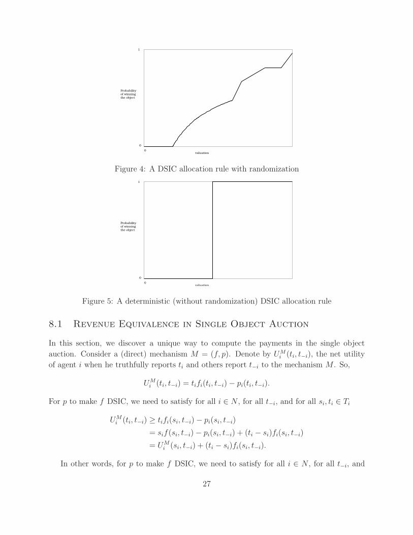
Consider an agent i ∈ N and fix the types of other agents at t−i. Figure 4 shows how

agent i’s probability of winning the object can change in a DSIC allocation rule. If we restrict

attention to DSIC allocation rules which either do not give the object to an agent or gives it

to an agent with probability 1, then the shape of the curve depicting probability of winning

the object will be a step function. We call such allocation rules deterministic allocation

rules. Figure 5 shows a deterministic DSIC allocation rule.

26

1

valuation0

Probabilityof winningthe object

0

Figure 4: A DSIC allocation rule with randomization

1

valuation0

Probabilityof winningthe object

0

Figure 5: A deterministic (without randomization) DSIC allocation rule

8.1 Revenue Equivalence in Single Object Auction

In this section, we discover a unique way to compute the payments in the single object

auction. Consider a (direct) mechanism M = (f, p). Denote by UMi (ti, t−i), the net utility

of agent i when he truthfully reports ti and others report t−i to the mechanism M . So,

UMi (ti, t−i) = tifi(ti, t−i) − pi(ti, t−i).

For p to make f DSIC, we need to satisfy for all i ∈ N , for all t−i, and for all si, ti ∈ Ti

UMi (ti, t−i) ≥ tifi(si, t−i) − pi(si, t−i)

= sif(si, t−i) − pi(si, t−i) + (ti − si)fi(si, t−i)

= UMi (si, t−i) + (ti − si)fi(si, t−i).

In other words, for p to make f DSIC, we need to satisfy for all i ∈ N , for all t−i, and

27

for all si, ti ∈ Ti, we must have

UMi (ti, t−i) − UM

i (si, t−i) ≥ (ti − si)fi(si, t−i).

If we fix i, t−i and si, ti ∈ Ti, we will get a pair of inequalities:

(ti − si)fi(ti, t−i) ≤ UMi (ti, t−i) − UM

i (si, t−i) ≤ (ti − si)fi(si, t−i).

Now, suppose Ti = [0, bi] for all i ∈ N . Consider ti = si + δ for some δ > 0. Then, the

previous pair of inequality reduces to

fi(si + δ, t−i) ≤UM

i (si + δ, t−i) − UMi (si, t−i)

δ≤ fi(si, t−i).

Letting δ → 0, we see that fi(si, t−i) is the slope of a line that supports the function UMi (·, t−i)

at si, i.e., fi(si, t−i) is a subgradient (subderivative) of the function UMi (·, t−i) at si. We know

that if p makes f DSIC, the f is non-decreasing. Further, UMi (·, t−i) is a convex function.

To see this, pick xi, zi ∈ Ti and consider yi = λxi + (1 − λ)zi for some λ ∈ (0, 1). We know

that

UMi (xi, t−i) ≥ UM

i (yi, t−i) + (xi − yi)fi(yi, t−i)

UMi (zi, t−i) ≥ UM

i (yi, t−i) + (zi − yi)fi(yi, t−i).

Adding these two we get

λUMi (xi, t−i) + (1 − λ)UM

i (zi, t−i) ≥ UMi (yi, t−i).

We know that a convex function is continuous in the interior of an interval. In fact, it is

absolutely continuous, and differentiable almost everywhere in the interior of its domain.

Since f is non-decreasing it is integrable. By the fundamental theorem of calculus, we can

write this function as the definite integral of its derivative.

UMi (ti, t−i) − UM

i (0, t−i) =

∫ ti

0

fi(xi, t−i)dxi

Substituting UMi (ti, t−i) = tifi(ti, t−i) − pi(ti, t−i) and UM

i (0, t−i) = −pi(0, t−i), we get

pi(ti, t−i) = pi(0, t−i) + tifi(ti, t−i) −

∫ ti

0

fi(xi, t−i)dxi

Notice that besides pi(0, t−i), the other terms on the right hand side is completely determined

by the allocation rule f . So, payment at any type profile is uniquely determined by f and

the payment pi(0, t−i). This is called the revenue equivalence theorem in single object

auction setting. It says that if we choose an allocation rule f which is DSIC, payments which

makes f DISC can differ by the payment at the lowest type only (i.e., pi(0, t−i) only).

28

An implication of this result is the following. Take two payment functions p and q that

make f DSIC. Then, for every i ∈ N and every t−i, we know that for every si, ti ∈ Ti,

pi(si, t−i) − pi(ti, t−i) =[

sifi(si, t−i) −

∫ si

0

fi(xi, t−i)dxi

]

−[

tifi(ti, t−i) −

∫ ti

0

fi(xi, t−i)dxi

]

and

qi(si, t−i) − qi(ti, t−i) =[

sifi(si, t−i) −

∫ si

0

fi(xi, t−i)dxi

]

−[

tifi(ti, t−i) −

∫ ti

0

fi(xi, t−i)dxi

]

Hence,

pi(si, t−i) − pi(ti, t−i) = qi(si, t−i) − qi(ti, t−i),

or pi(si, t−i) − qi(si, t−i) = pi(ti, t−i) − qi(ti, t−i).

8.2 Discovering the Vickrey Auction

Suppose f is the efficient allocation. We know that the class of Groves payments make f

DSIC. Suppose we impose the restriction that pi(0, t−i) = 0 for all i ∈ N and for all t−i.

Note that if ti is not the highest type in the profile, then fi(xi, t−i) = 0 for all xi ≤ ti.

Hence, pi(ti, t−i) = 0. If ti is the highest type and tj is the second highest type in the

profile, then fi(xi, t−i) = 0 for all xi ≤ tj and fi(xi, t−i) = 1 for all ti ≥ xi > tj . So,

pi(ti, t−i) = ti − [ti − tj] = tj. This is indeed the Vickrey auction. The revenue equivalence

result says that any other strategy-proof auction must have payments which differ from the

Vickrey auction by the amount a bidder pays at type 0, i.e., pi(0, t−i).

8.3 Deterministic Allocations Rules

Call an allocation rule f deterministic (in single object setting) if for all i ∈ N and every

type profile t, we have fi(t) ∈ 0, 1. The aim of this section is to show the simple nature of

payment rules for a deterministic allocation rule to be DSIC. We assume that set of types

of agent i is Ti = [0, bi]. Suppose f is a deterministic allocation rule which is DSIC. Hence,

it is non-decreasing. For every i ∈ N and every t−i, the shape of fi(·, t−i) is a step function

(as in Figure 5). Now, define,

κfi (t−i) =

infti ∈ Ti : fi(ti, t−i) = 1 if fi(ti, t−i) = 1 for some ti ∈ Ti

0 otherwise

If f is DSIC, then it is non-decreasing, which implies that for all ti > κfi (t−i), i gets the

object and for all ti < κfi (t−i), i does not get the object.

29

Consider a type ti ∈ Ti. If fi(ti, t−i) = 0, then using revenue equivalence, we can

compute any payment which makes f DSIC as pi(ti, t−i) = pi(0, t−i). If fi(ti, t−i) = 1, then

pi(ti, t−i) = pi(0, t−i) + ti − [ti − κfi (t−i)] = pi(0, t−i) + κ

fi (t−i). Hence, if p makes f DSIC,

then for all i ∈ N and for all t

pi(t) = pi(0, t−i) + κfi (t−i).

The payments when pi(0, t−i) = 0 has special interpretation. If fi(t) = 0, then agent i

pays nothing (losers pay zero). If fi(t) = 1, then agent i pays the minimum amount required

to win the object when types of other agents are t−i. If f is the efficient allocation rule, this

reduces to the second-price Vickrey auction.

We can also apply this to other allocation rules. Suppose N = 1, 2 and the allocations

are A = a0, a1, a2, where a0 is the allocation where the seller keeps the object, ai (i 6= 0)

is the allocation where agent i keeps the object. Given a type profile t = (t1, t2), the seller

computes, U(t) = max(2, t21, t32), and allocation is a0 if U(t) = 2, it is a1 if U(t) = t21, and a2

if U(t) = t32. Here, 2 serves as a (pseudo) reserve price below which the object is unsold. It

is easy to verify that this allocation rule is non-decreasing, and hence DSIC. Now, consider

a type profile t = (t1, t2). For agent 1, the minimum he needs to bid to win against t2

is√

max2, t32. Similarly, for agent 2, the minimum he needs to bid to win against t1 is

(max2, t21)13 . Hence, the following is a payment scheme which makes this allocation rule

DSIC. At any type profile t = (t1, t2), if none of the agents win the object, they do not pay

anything. If agent 1 wins the object, then he pays√

max2, t32, and if agent 2 wins the

object, then he pays (max2, t21)13 .

8.4 Individual Rationality

We can find out conditions under which a mechanism is individually rational. Notice that

the form of individual rationality we use is ex post individual rationality.

Lemma 3 Suppose a mechanism (f, p) is strategy-proof. The mechanism (f, p) is individu-

ally rational if and only if for all i ∈ N and for all t−i,

pi(0, t−i) ≤ 0.

Further a mechanism (f, p) is individually rational and pi(ti, t−i) ≥ 0 for all i ∈ N and for

all t−i if and only if for all i ∈ N and for all t−i,

pi(0, t−i) = 0.

Proof : Suppose (f, p) is individually rational. Then 0− pi(0, t−i) ≥ 0 for all i ∈ N and for

all t−i. For the converse, suppose pi(0, t−i) ≤ 0 for all i ∈ N and for all t−i. In that case,

ti − pi(ti, t−i) = ti − pi(0, t−i) − tifi(ti, t−i) +∫ ti0

fi(xi, t−i)dxi ≥ 0.

30

Individual rationality says pi(0, t−i) ≤ 0 and the requirement pi(0, t−i) ≥ 0 ensures

pi(0, t−i) = 0. For the converse, pi(0, t−i) = 0 ensures individual rationality.

Hence, individual rationality along with the requirement that payments are always non-

negative pins down pi(0, t−i) = 0 for all i ∈ N and for all t−i.

9 General Revenue Equivalence

Consider an allocation rule f which is DSIC. Let p be a payment rule which makes f DSIC.

Let hi be a function of agent i from the type profiles of agents other than i to R. Define such

family of functions (h1, . . . , hn). Define qi(t) = pi(t)+hi(t−i) for all i ∈ N and for all t ∈ T n.

Since qi(ti, t−i) − qi(si, t−i) = pi(ti, t−i) − pi(si, t−i) ≤ lt−i(si, ti) for every i ∈ N , for every

t−i, and for every si, ti, we see that q is also a payment that makes f DSIC. Is it possible

that there are payments other than those defined by various h functions? This property of

an allocation rule is called revenue equivalence. Not all allocation rules satisfy revenue

equivalence. As we have seen, in the standard auction of single object (one-dimensional type

space), every allocation rule satisfies revenue equivalence when type space of every agent

is a closed interval. The objective of this section is to identify allocation rules that satisfy

revenue equivalence in more general settings.

Definition 6 An allocation rule f satisfies revenue equivalence if for any two payment

rules p and p that make f DSIC, there exists functions hi : T−i → R for every agent i ∈ N

such that

pi(t) = pi(t) + hi(t−i) ∀ i ∈ N, ∀ t ∈ T n. (5)

The first characterization of revenue equivalence involves no assumptions on type spaces,

set of alternatives A, and v. The proof uses the following fact that we have used earlier.

Suppose f is DSIC. Then, we can determine a payment function using the underlying type

graphs. In particular, for every agent i and every t−i, we can define the the underlying

type graph Tf(t−i), where length of edge from si to ti is lTf (t−i)(si, ti) = vi(f(ti, t−i), ti) −

vi(f(si, t−i), ti). Denote the shortest path length from si to ti as distTf (t−i)(si, ti), where

distTf (t−i)(si, si) is assumed to be zero. Now, the following defines a payment function which

makes f DSIC:

pi(ti, t−i) = distTf (t−i)(si, ti).

The proof of this fact lies in the proof of Theorem 4.

Theorem 7 Suppose f is DSIC. Then the following are equivalent.

31

1. The allocation rule f satisfies revenue equivalence.

2. For all i ∈ N , for all t−i, and for all si, ti ∈ Ti, we have

distTf (t−i)(si, ti) + distTf (t−i)(ti, si) = 0.

Proof : Suppose f satisfies revenue equivalence. Fix agent i ∈ N and t−i. Consider any

si, ti ∈ Ti. Since f is DSIC, by Theorem 5, the following two payment rules make f DSIC:

psi

i (ri, t−i) = distTf (t−i)(si, ri) ∀ri ∈ Ti

ptii (ri, t−i) = distTf (t−i)(ti, ri) ∀ri ∈ Ti.

Since revenue equivalence holds, psi

i (si, t−i) − ptii (si, t−i) = psi

i (ti, t−i) − ptii (ti, t−i). But

psi

i (si, t−i) = ptii (ti, t−i) = 0. Hence, psi

i (ti, t−i)+ptii (si, t−i) = 0, which implies that distTf (t−i)(si, ti)+

distTf (t−i)(ti, si) = 0.

Now, suppose distTf (t−i)(si, ti) + distTf (t−i)(ti, si) = 0 for all si, ti ∈ Ti. Consider any

payment rule p that makes f DSIC. Fix si, ti ∈ Ti. Take any path P = (si, u1, . . . , uk, ti)

from si to ti in Tf(t−i). Now, l(P ) = l(si, u1) + l(u1, u2) + . . . + l(uk−1, uk) + l(uk, ti) ≥

[pi(u1, t−i)−pi(si, t−i)]+[pi(u

2, t−i)−pi(u1, t−i)]+. . .+[pi(u

k, t−i)−pi(uk−1, t−i)]+[pi(ti, t−i)−

pi(uk, t−i)] = pi(ti, t−i)−pi(si, t−i). Hence, pi(ti, t−i)−pi(si, t−i) ≤ l(P ) for any path P from

si to ti. Hence, pi(ti, t−i) − pi(si, t−i) ≤ distTf (t−i)(si, ti).

Similarly, pi(si, t−i)−pi(ti, t−i) ≤ distTf (t−i)(ti, si) = −distTf (t−i)(si, ti). Hence, pi(ti, t−i)−

pi(si, t−i) = distTf (t−i)(si, ti), which is independent of p(·). Now, consider two payment rules

p and q which makes f DSIC. By the above, any payment rule is determined by determining

payment of one of the nodes in the type graph. Fix a node si in type graph Tf(t−i). So, for

any type ti ∈ Ti, we know that

pi(ti, t−i) − pi(si, t−i) = qi(ti, t−i) − qi(si, t−i) = distTf (t−i)(si, ti).

This can be rewritten as

pi(ti, t−i) = qi(ti, t−i) + [pi(si, t−i) − qi(si, t−i)].

Since, [pi(si, t−i) − qi(si, t−i)] is independent of ti, we let hi(t−i) = [pi(si, t−i) − qi(si, t−i)].

This gives us,

pi(ti, t−i) = qi(ti, t−i) + hi(t−i).

Here is an example where one can verify revenue equivalence using this result. Consider

an economy with a single agent. The type space of this agent has T = s, t. The set of

32

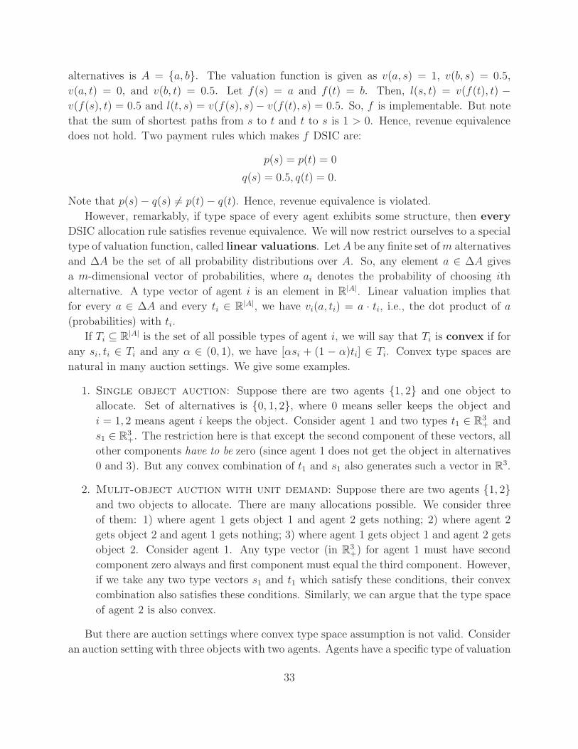
alternatives is A = a, b. The valuation function is given as v(a, s) = 1, v(b, s) = 0.5,

v(a, t) = 0, and v(b, t) = 0.5. Let f(s) = a and f(t) = b. Then, l(s, t) = v(f(t), t) −

v(f(s), t) = 0.5 and l(t, s) = v(f(s), s) − v(f(t), s) = 0.5. So, f is implementable. But note

that the sum of shortest paths from s to t and t to s is 1 > 0. Hence, revenue equivalence

does not hold. Two payment rules which makes f DSIC are:

p(s) = p(t) = 0

q(s) = 0.5, q(t) = 0.

Note that p(s) − q(s) 6= p(t) − q(t). Hence, revenue equivalence is violated.

However, remarkably, if type space of every agent exhibits some structure, then every

DSIC allocation rule satisfies revenue equivalence. We will now restrict ourselves to a special

type of valuation function, called linear valuations. Let A be any finite set of m alternatives

and ∆A be the set of all probability distributions over A. So, any element a ∈ ∆A gives

a m-dimensional vector of probabilities, where ai denotes the probability of choosing ith

alternative. A type vector of agent i is an element in R|A|. Linear valuation implies that

for every a ∈ ∆A and every ti ∈ R|A|, we have vi(a, ti) = a · ti, i.e., the dot product of a

(probabilities) with ti.

If Ti ⊆ R|A| is the set of all possible types of agent i, we will say that Ti is convex if for

any si, ti ∈ Ti and any α ∈ (0, 1), we have [αsi + (1 − α)ti] ∈ Ti. Convex type spaces are

natural in many auction settings. We give some examples.

1. Single object auction: Suppose there are two agents 1, 2 and one object to

allocate. Set of alternatives is 0, 1, 2, where 0 means seller keeps the object and

i = 1, 2 means agent i keeps the object. Consider agent 1 and two types t1 ∈ R3+ and

s1 ∈ R3+. The restriction here is that except the second component of these vectors, all

other components have to be zero (since agent 1 does not get the object in alternatives

0 and 3). But any convex combination of t1 and s1 also generates such a vector in R3.

2. Mulit-object auction with unit demand: Suppose there are two agents 1, 2

and two objects to allocate. There are many allocations possible. We consider three

of them: 1) where agent 1 gets object 1 and agent 2 gets nothing; 2) where agent 2

gets object 2 and agent 1 gets nothing; 3) where agent 1 gets object 1 and agent 2 gets

object 2. Consider agent 1. Any type vector (in R3+) for agent 1 must have second

component zero always and first component must equal the third component. However,

if we take any two type vectors s1 and t1 which satisfy these conditions, their convex

combination also satisfies these conditions. Similarly, we can argue that the type space

of agent 2 is also convex.

But there are auction settings where convex type space assumption is not valid. Consider

an auction setting with three objects with two agents. Agents have a specific type of valuation

33

called the single-minded valuations. Every agent i ∈ N has a desired bundle Si, if gets a

bundle S ⊇ Si, then he gets a value vi, else he gets zero. So, ant single-minded valuation

vector in R|A|+ will contain exactly one positive number. In the example, we consider three

allocations: 1) where agent 1 gets objects 1 and 2 and agent 2 gets object 3, 2) where agent

1 gets object 3 and agent 2 gets objects 1 and 2; 3) where agent 1 gets object 1 and agent

2 gets objects 2 and 3. Consider agent 1. One possible type vector is (5, 0, 0), where his

desired bundle is 1, 2 and value is 5. Another possible type vector is (10, 0, 10) where his

desired bundle is 1. But a convex combination of these two type vectors is (7.5, 0, 5), and

this is not a single-minded valuation because there are two positive numbers in this type

vector.

A consequence of the linear valuations and convex type space assumption is the following

lemma.

Lemma 4 (Path Contraction) Suppose the valuation function of every agent is linear and

Ti ∈ R|A| is convex for every i ∈ N . If f is DSIC, then for every i ∈ N and for every t−i the

following is true. For every si, ti ∈ Ti, and every ǫ > 0, there exists type vectors r1, r2, . . . , rk

such that

lt−i(si, r

1) + lt−i(r1, r2) + . . . + lt−i

(rk−1, rk) + lt−i(rk, ti) + lt−i

(ti, rk) + lt−i

(rk, rk−1)

+ . . . + lt−i(r1, si) < ǫ.

Proof : Let δ = ti − si (it is a vector in R|A|). Fix some integer k ≥ 1 and for every

j ∈ 1, . . . , k, define rj = si + jk+1

δ. Let r0 = si and rk+1 = ti. Because of convexity of Ti,

rj ∈ Ti for all j ∈ 1, . . . , k. Due to linear valuations, we can write for every j ∈ 1, . . . , k,

lt−i(rj, rj+1) = [f(rj+1, t−i) − f(rj, t−i)] · r

j+1

= [f(rj+1, t−i) − f(rj, t−i)] · si +j + 1

k + 1[f(rj+1, t−i) − f(rj, t−i)] · δ.

Similarly,

lt−i(rj+1, rj) = [f(rj, t−i) − f(rj+1, t−i)] · si +

j

k + 1[f(rj, t−i) − f(rj+1, t−i)] · δ.

Hence, we can write for every j ∈ 1, . . . , k,

lt−i(rj, rj+1) + lt−i

(rj+1, rj) =1

k + 1[f(rj+1, t−i) − f(rj, t−i)] · δ.

Hence, we can write,

k∑

j=0

[

lt−i(rj, rj+1 + lt−i

(rj+1, rj)]

=1

k + 1

[

f(ti, t−i) − f(si, t−i)]

· δ.

34

Since δ is fixed for given si and ti, we can make the right hand side arbitrarily small by

choosing large enough k. Hence, for any ǫ > 0, we can make

k∑

j=0

[

lt−i(rj, rj+1) + lt−i

(rj+1, rj)]

< ǫ.

This lemma leads to the main result.

Theorem 8 Suppose A is a finite set of alternatives and f : T n → ∆A be an allocation

rule. Further, let Ti ∈ R|A| be a convex set for every i ∈ N and valuation function of every

agent is linear. If f is DSIC, then it satisfies revenue equivalence.

Proof : Fix an agent i and type profile of other agents at t−i. By Theorem 7, we need to

show that for every si, ti ∈ Ti,

distTf (t−i)(si, ti) + distTf (t−i)(ti, si) = 0.

Since f is DSIC, it satisfies cycle monotonicity, which implies that distTf (t−i)(si, ti)+distTf (t−i)(ti, si) ≥

0. Assume for contradiction, distTf (t−i)(si, ti)+distTf (t−i)(ti, si) = ǫ > 0. By Lemma 4, there

exists paths from si to ti and from ti to si such that sum of their lengths is < ǫ. Hence,

distTf (t−i)(si, ti) + distTf (t−i)(ti, si) < ǫ. This is a contradiction.

10 Bayesian Incentive Compatibility

Bayesian incentive compatibility was introduced in Harsanyi (1967-68). It is a weaker re-

quirement than the dominant strategy incentive compatibility. While dominant strategy

incentive compatibility required the equilibrium strategy to be the best strategy under all

possible strategies of opponents, Bayesian incentive compatibility requires this to hold in

expectation. This means that in Bayesian incentive compatibility, an equilibrium strategy

must give the highest expected utility to the agent, where we take expectation over types of

other agents. To be able to take expectation, agents must have information about the prob-

ability distributions from which types of other agents are drawn. Hence, Bayesian incentive

compatibility is informationally demanding. In dominant strategy incentive compatibility

the mechanism designer needed information on the type space of agents, and every agent

required no prior information of other agents. In Bayesian incentive compatibility, every

agent and the mechanism designer needs to know the distribution from which agents’ types

are drawn.

To understand Bayesian incentive compatibility, fix a mechanism (M, g). A Bayesian

strategy for such a mechanism is a vector of mappings mi : Ti → Mi for every i ∈ N . A

35

profile of such mapping m : T n → M is a Bayesian equilibrium if for all i ∈ N , for all

ti ∈ Ti, and for all mi ∈ Mi we have

E−i

[

vi(ga(m−i(t−i), mi(ti)), ti) + gi(m−i(t−i), mi(ti))|ti]

≥

E−i

[

vi(ga(m−i(t−i), mi)), ti) + gi(m−i(t−i), mi)|ti]

,

where E−i[·] denotes the expectation over type profile t−i conditional on the fact that i has

type ti. If all tis are drawn independently, then we need not condition in the expectation.

A direct mechanism (social choice function) (f, p) is Bayesian incentive compatible

if mi(ti) = ti for all i ∈ N and for all ti ∈ Ti is a Bayesian equilibrium, i.e., for all i ∈ N and

for all ti, ti ∈ Ti we have

E−i

[

vi(f(t−i, ti), ti) + pi(t−i, ti)|ti]

≥ E−i

[

vi(f(t−i, ti), ti) + pi(t−i, ti)|ti]

A dominant strategy incentive compatible mechanism is Bayesian incentive compatible. A

mechanism (M, g) realizes a social choice function (f, p) in Bayesian equilibrium if there

exists a Bayesian equilibrium m : T n → M of (M, g) such that ga(m(t)) = f(t) and gi(t) =

pi(t) for all i ∈ N and for all t ∈ T n. Analogous to the revelation principle for dominant

strategy incentive compatibility, we also have a revelation principle for Bayesian incentive

compatibility.

Proposition 2 (Revelation Principle) If a mechanism (M, g) realizes a social choice

function F = (f, p) in Bayesian equilibrium, then the direct mechanism F = (f, p) is

Bayesian incentive compatible.

11 Optimal Auction Design

This section will describe the design of optimal auction for selling a single indivisible object

to a set of bidders (buyers) who have quasi-linear utility functions. The seminal paper in

this area is (Myerson, 1981). We present a detailed analysis of this work. Before I describe

the formal model, let me describe some popular auction forms used in practice.

11.1 Auctions for a Single Indivisible Object

A single indivisible object is for sale. Let us consider four bidders (agents or buyers) who

are interested in buying the object. Let the valuations of the bidders be 10, 8, 6, and 4

respectively. Let us discuss some commonly used auction formats using this example. As

before, let us assume agents/bidders have quasi-linear utility functions and private values.

36

• Posted price: The seller announces a price at which he will sell the object. The first

buyer to express demand at this price wins the object. It is a very common form of

selling. Since the seller does not elicit any information from the buyers, this makes

sense if the seller has good information about the values of buyers to set his price.

• First-price auction: In the first-price auction, every bidder is asked to report a bid,

which indicates his value. The highest bidder wins the auction and pays the price he

bid. Of course, the bid amount need not equal the value. But if the bidders bid their

value, then the first bidder will win the object and pay an amount of 10.

• Second-price auction: In the second-price auction, like the first-price auction, each

bidder is asked to report a bid. The highest bidder wins the auction and pays the price

of the second highest bid. This is the Vickrey auction we have already discussed. As

we saw, a dominant strategy in this auction is that bidders will bid their values. Hence,

the first bidder will win the object but pay a price equal to 8, the second highest value.

• Dutch auction: The Dutch auction, popular for selling flowers in the Netherlands,

falls into a class of auctions called the open-cry auctions. The Dutch auction starts at

a high price and the price of the object is lowered by a small amount (called the bid

decrement) in iterations. In every iteration, bidders can express their interest to buy

the object. The price of the object is lowered only if no bidder shows interest. The

auction stops as soon as any bidder shows interest. The first bidder to show interest

wins the object at the current price.

In the example above, suppose the Dutch auction is started at price 12 and let the bid

decrement be 1. At price 12, no bidder should express interest since valuation of all

bidders are less than 12. After price 10, the first bidder may choose to express interest

since he starts getting non-negative utility from the object for any price less than or

equal to 10. If he chooses to express interest, then the auction would stop and he will

win the object. Clearly, it is not an equilibrium for the bidder to express interest at

10 since he can potentially get more payoff by waiting for the price to fall. Indeed, in

equilibrium (under some conditions), the bidder will show interest at a price just below

his valuation.

• English auction: The English auction is also an open-cry auction. The seller starts

the auction at a low price and raises it by a small amount (called the bid increment)

in iterations. In every iteration, like in the Dutch auction, the bidders are asked if

they are interested in buying the object. The price is raised only if more than one

bidder shows interest. The auction stops as soon as one or less number of bidders show

interest. The last bidder to show interest wins the auction at the price he last showed

interest.

37

In the example above, suppose the English auction is started at price 0 and let the bid

increment be 1. Then, at price 4 the bidder with value 4 will stop showing interest

(since he starts getting non-positive payoff from that price onwards). Similarly, at

prices 6, bidder with value 6 will drop out. Finally, bidder with value 8 will drop out

at price 8. At this price, only bidder with value 10 will show interest. Hence, the

auction will stop at price 8, and the bidder with value 10 will win the object at price 8.

Notice that the outcome of the auction is the same as the second-price auction. This is

no coincidence. It can be argued easily that it is an equilibrium (under private values

model) for bidders to show interest (bid) till the price reaches their value in the English

auction. Hence, the outcome of the English auction is the same as the second-price

auction.

One can think of many more auction formats - though they may not be used in practice.

Having learnt and thought about these auction formats, some natural questions arise. Is there

an equilibrium strategy for the bidder in each of these auctions? What kind of auctions are

incentive compatible? What is the ranking of these auctions in terms of expected revenue?

Which auction gives the maximum expected revenue to the seller over all possible auctions?

Myerson (1981) answers many of these questions. First, using the revelation principle

(for Bayesian incentive compatibility), he concludes that for every auction (sealed-bid or

open-cry or others) there exists a direct mechanism with the same social choice function,

and thus giving the same expected revenue to the seller. So, he focuses on direct mechanisms

without loss of generality. Second, he characterizes direct mechanisms which are Bayesian

incentive compatible. Third, he shows that all Bayesian incentive compatible mechanisms

which have the same allocation rule, differ in revenue by a constant amount. Using these

results, he is able to give a precise description of an auction which gives the maximum

expected revenue. He calls such an auction an optimal auction. Under some conditions on

the valuation distribution of bidders, the optimal auction is a modified second-price auction.

Next, we describe these results formally.

11.2 The Model

There is a single indivisible object for sale, whose value for the seller is zero. The set of bidders

is denoted by N = 1, . . . , n. Every bidder has a value (this is his type) for the object. The

value of bidder i ∈ N is drawn from [0, bi] using a distribution with density function fi and

cumulative density Fi. We assume that each bidder draws his value independently and this

value is completely determined by this draw (i.e., knowledge of other information such as

value of other bidders does not influence his value). This model of valuation is referred to

as the private independent value model. We let the joint density function of values of

all the bidders as f and the joint density function of values of all the bidders except bidder

38

i as f−i. Due to the independence assumption, for every profile of values x = (x1, . . . , xn)

f(x1, . . . , xn) = f1(x1) × . . . × fn(xn)

f−i(x1, . . . , xi−1, xi+1, . . . , xn) = f1(x1) × . . . × fi−1(xi−1) × fi+1(xi+1) × . . . fn(xn).

Let Xi = [0, bi] and X = [0, b1] × . . .× [0, bn]. Similarly, let X−i = ×j∈N\iXj . A typical

valuation of bidder i will be denoted as xi ∈ Xi, a valuation profile of bidders will be denoted

as x ∈ X, and a valuation profile of bidders in N \ i will be denoted as x−i ∈ X−i. The

valuation profile x = (x1, . . . , xi, . . . , xn) will sometimes be denoted as (xi, x−i). We assume

that fi(xi) > 0 for all i ∈ N and for all xi ∈ Xi.

11.3 The Direct Mechanisms

Though a mechanism can be very complicated, a direct mechanism is simpler to describe.

By virtue of the revelation principle (Proposition 2), we can restrict attention to direct

mechanisms only. Henceforth, I will refer to a direct mechanism as simply a mechanism.

Let A be the set of all deterministic allocation rules, i.e., A = a0, a1, . . . , an, where a0

is the allocation where the seller keeps the object and ai for 1 ≤ i ≤ n denotes the allocation

where agent i gets the object. Let ∆A be the set of all probability distributions over A. A

direct mechanism Γ in this context is a pair of mappings Γ = (a, p), where a : X → ∆A is

the allocation rule and p : X → Rn is the payment rule. Given a mechanism Γ = (a, p),

a bidder i ∈ N with (true) value xi ∈ Xi gets the following utility when all the buyers report

values z = (z1, . . . , zi, . . . , zn)

ui(z; xi) = ai(z)xi − pi(z),

where ai(z) is the probability that agent i gets the object at bid profile z and pi(z) is the

payment of agent i at bid profile z. Every mechanism (a, p) induces an expected allocation

rule and an expected payment rule (α, π), defined as follows. The expected allocation of

bidder i when he reports zi ∈ Xi in allocation rule a is

αi(zi) =

∫

X−i

ai(zi, z−i)f−i(z−i)dz−i.

Similarly, the expected payment of bidder i when he reports zi ∈ Xi in payment rule p is

πi(zi) =

∫

X−i

pi(zi, z−i)f−i(z−i)dz−i.

So, the expected utility from a mechanism (a, p) to a bidder i with true value xi by reporting

a value zi is αi(zi)xi − πi(zi).

39

Definition 7 A mechanism (a, p) is Bayesian incentive compatible (BIC) if for every

bidder i ∈ N and for every possible value xi ∈ Xi we have

αi(xi)xi − πi(xi) ≥ αi(zi)xi − πi(zi) ∀ zi ∈ Xi. (BIC)

Equation BIC says that a bidder maximizes his expected utility by reporting true value. So,

when bidder i has value xi, he gets more expected utility by reporting xi than by reporting

any other value zi ∈ Xi.

11.4 Bayesian Incentive Compatible Allocation Rules

We say an allocation rule a is Bayesian incentive compatible if there exists a payment rule

p such that (a, p) is a Bayesian incentive compatible mechanism. In other words, we must

find p : X → Rn such that for all i ∈ N , we have

πi(xi) − πi(zi) ≤ [αi(xi) − αi(zi)]xi ∀ xi, zi ∈ Xi. (6)

We say that an allocation rule a is non-decreasing in expectation (NDE) if for

all i ∈ N and for all xi, zi ∈ Xi with xi < zi we have αi(xi) ≤ αi(zi). Similar to the

characterization in the dominant strategy case, we have a characterization in the Bayesian

incentive compatible case.

Theorem 9 An allocation rule is Bayesian incentive compatible if and only if it is NDE.

Proof : For the proof, we give a graph theoretic representation of inequalities in Equation

6. For agent i ∈ N , consider a graph Gai , call it type graph of agent i, where the set of

nodes is Xi and there is an edge from every xi ∈ Xi to every other zi 6= xi. The length of

edge from zi to xi is defined as:

li(zi, xi) = [αi(xi) − αi(zi)]xi.

Hence, the inequalities 6 can be written for agent i ∈ N as

πi(xi) − πi(zi) ≤ li(zi, xi) ∀ xi, zi ∈ Xi.

Hence, allocation rule a is Bayesian incentive compatible if and only if for every i ∈ N , there

exists a potential in the type graph Gai . By our earlier result, a potential in type graph Ga

i

exists if and only if there is no cycle of negative length in Gai .

Now, we use the steps in the proof of characterization of dominant strategy incentive

compatible allocation rules here to conclude that no cycle of negative length is equivalent to

requiring that allocation rule is NDE.

40

Throughout the proof, we fix an agent i ∈ N . To simplify notation, we suppress i from

notations. We examine the type graph Gai .

Suppose a is BIC. Then, consider any s, t ∈ X with s > t. By no cycle of negative length

characterization, l(s, t) + l(t, s) ≥ 0. Hence,

[α(t) − α(s)](t − s) ≥ 0.

Since s > t, we get α(t) ≤ α(s). Hence a is NDE.

Suppose a is NDE. To show that a is BIC, we need to show that length of any cycle

having finite number of nodes (types) in Ga is non-negative. We use induction on number

of nodes involved in a cycle.

First note that for any s, t ∈ T , s > t implies that α(s) ≥ α(t), and this implies that

l(s, t) = [α(t) − α(s)]t ≥ [α(t) − α(s)]s = −l(t, s). Hence, l(s, t) + l(t, s) ≥ 0. So, any cycle

involving two nodes has non-negative length.

Now consider a cycle with (k + 1) nodes, and assume that any cycle involving less than

(k + 1) nodes has non-negative length. Let the cycle be (t1, t2, . . . , tk+1), and let, without

loss of generality, tk+1 > tj for all j ∈ 1, . . . , k. We first show that l(tk, tk+1)+ l(tk+1, t1) ≥

l(tk, t1). This will enable us to show that the length of this cycle is greater than or equal to

the length of cycle (t1, . . . , tk, t1), which has k nodes, and we will be done by the induction

hypothesis.

Assume for contradiction l(tk, tk+1) + l(tk+1, t1) < l(tk, t1). Then,

[α(tk+1) − α(tk)]tk+1 + [α(t1) − α(tk+1)]t1 < [α(t1) − α(tk)]t1,

or [α(tk+1) − α(tk)]tk+1 < [α(tk+1) − α(tk)]t1. (7)

Since tk+1 > t1 and tk+1 > tk implies α(tk+1) ≥ α(tk) by NDE, Equation 3 gives a contradic-

tion. Hence, l(tk, tk+1) + l(tk+1, t1) ≥ l(tk, t1).

Now, the length of the cycle (t1, t2, . . . , tk+1, t1) is l(t1, t2)+ . . .+ l(tk, tk+1)+ l(tk+1, t1) ≥

l(t1, t2) + . . . + l(tk−1, tk) + l(tk, t1). But the term in the right is the length of the cycle

(t1, t2, . . . , tk, t1), which has k nodes. By induction hypothesis, the length of this cycle is

non-negative. Hence, l(t1, t2) + . . . + l(tk, tk+1) + l(tk+1, t1) ≥ 0.

Note that NDE guarantees existence of expected payment rule. But we can use the same

payment in every profile of other types to generate a payment rule. Hence, existsnce of an

expected payment rule (π) also guarantees existence of a payment rule (p).

A BIC allocation rule need not be DSIC. We give an example to illustrate this. Consider

a setting with two agents N = 1, 2. Suppose the values of both the agents are drawn

uniformly from [0, 1]. Figure 6 shows an allocation rule a. The type profiles are divided into

cells of equal size (25 of them in total). Some of the cells are assigned some numbers - this

is the probability with which agent 1 gets the object in a. The cells in which no number

41

2/5

v1

v2

1

1

0 0 1

1 1

1

1

0

1

3/51/500

0

Figure 6: A BIC allocation rule which is not DSIC

is written, the probability of agent 1 getting the object at those profiles is zero. For our

purpose, the probability of agent 2 getting the object is irrelevant - for simplicity, we can

assume it to zero or we can put probabilities such that it is non-decreasing in expectation

(there are many ways to do it in this example).

The numbers on the x-axis indicate the expected probability of agent 1 getting the object

in allocation rule a. It is easy to verify that a is not non-decreasing but the expected

probability of agent 1 is non-decreasing, i.e., a is non-decreasing in expectation. Hence, the

allocation rule a is BIC but not DSIC.

11.5 Payments and Revenue Equivalence

The next theorem states a powerful fact about the payments in a Bayesian incentive com-

patible mechanism. It says that once we fix an NDE allocation rule, the payment rule is

uniquely determined upto an additive constant. This is known as the revenue equivalence

result, and proved in Myerson (1981). Note that if (a, p) is BIC, then by adding a constant

α to π also generates another payment rule which makes a BIC. The power of this result is

that it is the only way to generate the payments. Besides, it gives a precise formula on how

to generate these payments.

Theorem 10 (Revenue Equivalence) Suppose (a, p) is Bayesian incentive compatible.

42

Then, for every bidder i ∈ N and every xi ∈ Xi we have

πi(xi) = πi(0) + αi(xi)xi −

∫ xi

0

αi(ti)dti.

Proof : For every i ∈ N and every xi ∈ Xi denote Ui(xi) = αi(xi)xi − πi(xi). Consider a

bidder i ∈ N and xi, zi ∈ Xi. Since (a, p) is Bayesian incentive compatible, we can write

Ui(xi) ≥ αi(zi)xi − πi(zi)

= αi(zi)(xi − zi) + αi(zi)zi − πi(zi)

= Ui(zi) + αi(zi)(xi − zi).

Switching the role of xi and zi we get

Ui(zi) ≥ Ui(xi) + αi(xi)(zi − xi).

Hence, we can write

αi(xi)(zi − xi) ≤ Ui(zi) − Ui(xi) ≤ αi(zi)(zi − xi).

Let zi = xi + δ for δ > 0. Then, we get

αi(xi)δ ≤ Ui(xi + δ) − Ui(xi) ≤ αi(xi + δ)δ.

It is clear that Ui(·) is a continuous function. Also, αi(xi) is the slope of a line that supports

Ui(·) at xi. Using the fundamental theorem of calculus, and the fact that αi(·) is Riemann

integrable since it is non-decreasing, we can write

∫ xi

0

αi(ti)dti = Ui(xi) − Ui(0).

Substituting Ui(0) = −πi(0) and Ui(xi) = αi(xi)xi − πi(xi), we get

∫ xi

0

αi(ti)dti = αi(xi)xi − πi(xi) + πi(0).

This gives us the desired inequality

πi(xi) = πi(0) + αi(xi)xi −

∫ xi

0

αi(ti)dti.

Theorem 10 says that the (expected) payment of a bidder in a mechanism is uniquely

determined by the allocation rule once we fix the expected payment of a bidder with the

43

lowest type. Hence, a mechanism is uniquely determined by its allocation rule and the

payment of a bidder with the lowest type.

It is instructive to examine the payment function when πi(0) = 0. Then payment of

agent i at type xi becomes πi(xi) = αi(xi)xi −∫ xi

0αi(ti)dti. Because of non-decreasing αi(·)

function this is always greater than or equal to zero - it is the difference between area of the

rectangle with sides αi(xi) and xi and the area under the curve αi(·) from 0 to xi.

We next impose a condition on the mechanism which determines the payment of a bidder

when he has the lowest type.

Definition 8 A mechanism (a, p) is individually rational if for every bidder i ∈ N we

have αi(xi)xi − πi(xi) ≥ 0 for all xi ∈ Xi.

This form of individual rationality is weaker than ex post individual rationality that we

used earlier. This is commonly referred to as the interim individual rationality. Notice that

if (a, p) is Bayesian incentive compatible and individually rational, then πi(0) ≤ 0 for all

i ∈ N . As we will see, the optimal auction has πi(0) = 0, and thus πi(xi) ≥ 0 for all xi ∈ Xi,

i.e., biddders pay the auctioneer. This is a standard feature of many auctions in practice

where bidders are never paid.

11.6 Optimal Mechanisms

Denote the expected revenue from a mechanism (a, p) as

Π(a, p) =∑

i∈N

∫ bi

0

πi(xi)fi(xi)dxi.

We say a mechanism (a, p) is an optimal mechanism if

• (a, p) is Bayesian incentive compatible and individually rational,

• and Π(a, p) ≥ Π(a′, p′) for any other Bayesian incentive compatible and individually

rational mechanism (a′, p′).

Fix a mechanism (a, p) which is Bayesian incentive compatible and individually rational.

For any bidder i ∈ N , the expected payment of bidder i ∈ N is given by∫ bi

0

πi(xi)fi(xi)dxi = πi(0) +

∫ bi

0

αi(xi)xifi(xi)dxi −

∫ bi

0

∫ xi

0

(

αi(ti)dti)

fi(xi)dxi,

where the last equality comes by using revenue equivalence (Theorem 10). By interchanging

the order of integration in the last term, we get∫ bi

0

∫ xi

0

(

αi(ti)dti)

fi(xi)dxi =

∫ bi

0

(

∫ bi

ti

fi(xi)dxi

)

αi(ti)dti

=

∫ bi

0

(1 − Fi(ti))αi(ti)dti.

44

Hence, we can write

Π(a, p) =∑

i∈N

πi(0) +∑

i∈N

∫ bi

0

(

xi −1 − Fi(xi)

fi(xi)

)

αi(xi)fi(xi)dxi.

We now define the virtual valuation of bidder i ∈ N with valuation xi ∈ Xi as

wi(xi) = xi −1 − Fi(xi)

fi(xi).

Note that since fi(xi) > 0 for all i ∈ N and for all xi ∈ Xi, the virtual valuation wi(xi) is

well defined. Also, note that virtual valuations can be negative. Using this and the definition

of αi(·), we can write

Π(a, p) =∑

i∈N

πi(0) +∑

i∈N

∫ bi

0

wi(xi)αi(xi)fi(xi)dxi

=∑

i∈N

πi(0) +∑

i∈N

∫ bi

0

(

∫

X−i

ai(xi, x−i)f−i(x−i)dx−i

)

wi(xi)fi(xi)dxi

=∑

i∈N

πi(0) +∑

i∈N

∫

X

wi(xi)ai(x)f(x)dx

=∑

i∈N

πi(0) +

∫

X

(

∑

i∈N

wi(xi)ai(x))

f(x)dx.

We need to maximize Π(a, p) subject to Bayesian incentive compatibility and individual

rationality constraints. Let us sidestep Bayesian incentive compatibility constraint

for the moment. So, we are only concerned about maximizing

Π(a, p) =∑

i∈N

πi(0) +

∫

X

(

∑

i∈N

wi(xi)ai(x))

f(x)dx, (8)

subject to individual rationality constraint. Individual rationality implies that πi(0) ≤ 0 for

all i ∈ N . Hence, if we want to maximize Π(a, p), then πi(0) = 0 for all i ∈ N .

A careful look at the second term on the right hand side of Equation 8 is necessary.

Consider a profile of valuations x ∈ X. Consider∑

i∈N wi(xi)ai(x) for a valuation profile

x ∈ X. This is maximized by setting ai(x) = 1 if wi(xi) = maxj∈N wj(xj) ≥ 0, else setting

ai(x) = 0 for all i ∈ N . That is, we allocate the object to the buyer with the highest

non-negative virtual valuation (breaking ties arbitrarily), and we do not allocate the object

if the highest virtual valuation is negative. This way, we will maximize∑

i∈N wi(xi)ai(x),

and hence will maximize∑

i∈N wi(xi)ai(x)f(x). This in turn will maximize the second term

on the right hand side of Equation 8.

Now, we come back to Bayesian incentive compatibility requirement, which we had

sidestepped. By virtue of Theorem 9, we need to ensure that the suggested allocation

45

here

All BIC and IR randomized mechanisms

BIC and IRdeterministicmechanisms

DSIC and IRrandomizedmechanisms

OptMech

Figure 7: Optimal mechanism is DSIC, IR, and deterministic

rule is NDE. In general, it is not NDE. However, it is NDE under the following condition.

We say the regularity condition holds if for every bidder i ∈ N , for all xi > zi we have

wi(xi) > wi(zi), i.e., wi(·) is an increasing function. Note that regularity is satisfied if for all

i ∈ N and for all xi > zi, we have 1−Fi(xi)fi(xi)

≤ 1−Fi(zi)fi(zi)

. The term fi(xi)1−Fi(xi)

is called the hazard

rate. So, regularity is satisfied if the hazard rate is non-decreasing. To see this consider

xi > zi. By definition xi −1−Fi(xi)

fi(xi)> zi −

1−Fi(zi)fi(zi)

or wi(xi) > wi(zi).

The uniform distribution satisfies the regularity condition. Because 1−Fi(xi)fi(xi)

= bi − xi,

which is non-increasing in xi. For the exponential distribution, f(x) = µe−µx and F (x) =

1 − e−µx. Hence, 1−Fi(xi)fi(xi)

= 1µ, which is a constant. So, the exponential distribution also

satisfies the regularity condition.

If the regularity condition holds, then a is NDE. To see this, consider a bidder i ∈ N

and xi, zi ∈ Xi with xi > zi. Regularity gives us wi(xi) > wi(zi). By the definition of

the allocation rule, for all x−i ∈ X−i, we have ai(xi, x−i) ≥ ai(zi, x−i). Hence, a is NDE.

Moreover, a is non-decreasing, and hence DSIC. Further, a is a deterministic allocation rule.

We already know how to compute the payments corresponding to a deterministic DSIC

allocation rule such that IR constraints are satisfied.

Figure 7 highlights the fact that we started out searching for an optimal mechanism in

a large family of BIC, IR, and randomized mechanisms. But the optimal mechanism turned

out to be DSIC, IR, and deterministic.

If the regularity condition does not hold, the optimal mechanism is more complicated,

and you can refer to Myerson’s paper for a complete treatment.

The associated payment for bidder i ∈ N for a profile of valuation x can be computed

using revenue equivalence by using the fact that pi(0, x−i) = 0 for all i ∈ N and for all x−i.

Hence, for all i ∈ N and for all x ≡ (x1, . . . , xn), the payment of bidder i is computed using

the following expression

pi(x) = ai(x)xi −

∫ xi

0

ai(ti, x−i)dti

46

..............................................................................................................................................................................................................................................................................................................................................................................................................................................................................................................................................

..............................................................................................................................................................................................................................................................................................................................................................................................................................................................................................................................................

.......................................................................................................................................................................................................................................................................................................................................................................

0

1

0κi(x−i) bi

ai(xi, x−i)

xi: Value of bidder i

Figure 8: Allocation in optimal mechanism

Note that this payment makes the allocation rule a DSIC. Further, we know that it satisfies

stronger version of individual rationality. Hence, it must make a BNIC and IR.

This describes an optimal mechanism. From Equation 8 and the description of the

optimal mechanism, the expected highest revenue is the expected value of the highest virtual

valuation provided it is non-negative.

This mechanism can be simplified further (this simplification is something we have already

seen before - computing payments for a deterministic DSIC allocation rule using thresholds).

Define for all i ∈ N and all x−i ∈ X−i

κi(x−i) = infzi : wi(zi) ≥ 0 and wj(xj) ≤ wi(zi) ∀ j 6= i.

Hence, κi(x−i) is the valuation whose corresponding virtual valuation is non-negative and

“beats” the virtual valuations of other bidders. Thus the optimal allocation rule under

regularity condition satisfies, for all i ∈ N , for all zi ∈ Xi, and for all x−i ∈ X−i,

ai(zi, x−i) = 1 if zi > κi(x−i)

ai(zi, x−i) = 0 if zi < κi(x−i).

At zi = κi(x−i), the seller sells the object, but there may be more than one buyer with highest

virtual valuation. So, ai(zi, x−i) may be zero or one. Thus, one of the optimal mechanisms

has the feature where ai(x) ∈ 0, 1 for every i ∈ N and for every x ∈ X. The allocation is

shown in Figure 8.

47

Hence, for all i ∈ N , for all xi ∈ Xi, and for all x−i ∈ X−i

∫ xi

0

ai(zi, x−i)dzi = xi − κi(x−i) if xi ≥ κi(x−i)

∫ xi

0

ai(zi, x−i)dzi = 0 if xi < κi(x−i).

Hence, if ai(x) = 1, then pi(x) = xi −∫ xi

0ai(ti, x−i)dti = xi − (xi − κi(x−i)) = κi(x−i) and if

ai(x) = 0, pi(x) = 0. This simplifies the payment rule. For all i ∈ N , for all xi ∈ Xi, and for

all x−i ∈ X−i

pi(x) = κi(x−i) if ai(x) = 1

pi(x) = 0 if ai(x) = 0.

Thus, the optimal mechanism is the following auction. We order the virtual valuations of

bidders. Award the object to the highest non-negative virtual valuation bidder (breaking ties

arbitrarily - ties will happen with probability zero), and the winner, if any, pays the valuation

corresponding to the second highest virtual valuation, while the losers pay nothing. In other

words, the seller sets a reserve price 4 for bidder i, equal to infzi ∈ Xi : wi(zi) ≥ 0, and

for the bidders whose valuations exceed the respective reserve prices, he conducts the above

auction. This leads to the seminal result in (Myerson, 1981).

Theorem 11 (Optimal Auction) Suppose the regularity condition holds. Then, the fol-

lowing mechanism is optimal. The allocation rule a satisfies∑

i∈N ai(x) = 1 if and only if

maxi∈N wi(x) ≥ 0 and for all i ∈ N with wi(xi) ≥ 0 we must have,

ai(x) = 1 if wi(xi) > maxj 6=i

wj(xj)

ai(x) = 0 if wi(xi) < maxj 6=i

wj(xj),

and ai(x) = 0 for all i ∈ N with wi(x) < 0. The payment rule p is given by

pi(x) = κi(x−i) if ai(x) = 1

pi(x) = 0 if ai(x) = 0.

Figure 9 describes the working of the mechanism for a two bidder example. The virtual

valuation functions w1 and w2 are drawn. The reserve prices, r1 = w−11 (0) and r2 = w−1

2 (0)

are shown. For given values (x1, x2), we notice that x1 > r1 and x2 > r2, and by regularity,

w1(x1) > 0 and w2(x2) > 0. Hence, both the bidders are in contention for winning the

object. But w1(x1) > w2(x2). So, bidder 1 wins the object and pays a price equal to κ1(x2).

4A reserve price in an auction indicates that if bids are less than the reserve price than the object will

not be sold.

48

Virtualvalue ofbidder 1

Virtual valueof bidder 2

Value of bidder 1 Value of bidder 2

k_1(x_2) x_1 x_2

Figure 9: Illustration of the optimal mechanism

11.6.1 Symmetric Bidders

Finally, we look at the special case where the buyers are symmetric, i.e., they draw the

valuations using the same distribution - fi = f and X1 = X2 = . . . = Xn for all i ∈ N . So,

virtual valuations are the same: wi = w for all i ∈ N . In this case w(xi) > w(xj) if and only

if xi > xj by regularity. Hence, maximum virtual valuation corresponds to the maximum

valuation.

Thus, κi(x−i) = maxw−1(0), maxj 6=i xj. This is exactly, the second-price auction with

the reserve price of w−1(0). Hence, when the buyers are symmetric, then the second-price

auction with a reserve price equal to w−1(0) is optimal.

11.6.2 An Example

Consider a setting with two buyers whose values are distributed uniformly in the intervals

X1 = [0, 12] (buyer 1) and X2 = [0, 18] (buyer 2). Virtual valuation functions of buyer 1 and

buyer 2 are given as:

w1(x1) = x1 −1 − F1(x1)

f1(x1)= x1 − (12 − x1) = 2x1 − 12

w2(x2) = x2 −1 − F2(x2)

f2(x2)= x2 − (18 − x2) = 2x2 − 18.

Hence, the reserve prices for both the bidders are respectively r1 = 6 and r2 = 9. The

optimal auction outcomes are shown for some instances in Table 3.

49

Valuations Allocation (who gets object) Payment of Buyer 1 Payment of Buyer 2

(x1 = 4, x2 = 8) Object not sold 0 0

(x1 = 2, x2 = 12) Buyer 2 0 9

(x1 = 6, x2 = 6) Buyer 1 6 0

(x1 = 9, x2 = 9) Buyer 1 6 0

(x1 = 8, x2 = 15) Buyer 2 0 11

Table 3: Description of Optimal Mechanism

11.6.3 Efficiency and Optimality

Typically, the optimal mechanism is inefficient. There are two sources of inefficiency. One is

the asymmetric bidders. Consider two bidders who draw their values uniformly from [0, 10]

and [0, 6] respectively. We know that a uniform distribution with interval [0, h] has a virtual

valuation function w(x) = x − (h − x) = 2x − h. Consider the case when the values of the

bidders are (6, 5) respectively. Then the virtual value of the first bidder is 12− 10 = 2. The

virtual value of the second bidder is 10 − 6 = 4. Hence, the second bidder wins the object

even if he is not the highest bidder.

The other source of inefficiency is the reserve price. Consider the case of a single bidder

with values drawn uniformly from [0, 100]. The optimal auction is to sell the object when

value x satisfies 2x − 100 ≥ 0 or x ≥ 50. Hence, the object is not sold even at positive

values when value is less than 50. This is inefficient. To see how it is an improvement over

efficiency, notice that if the object is always sold, then the bidder would always pay zero,

resulting in expected revenue of zero. On the other hand, raising the reserve price too high

will result in no sale, and hence zero revenue. So, the optimal reserve price is somewhere in

between.

On the other hand, by putting a reserve price, he pays zero when he does not win (x < 50)

and pays the reserve price 50 when he wins (x ≥ 50). So, expected revenue is 25.

However, the optimal mechanism is efficient in a different sense. When bidders are

symmetric, the optimal mechanism sells the object efficiently whenever it sells. Though

the second-price auction is rarely used in practice, but is weakly equivalent to the popular

English auction. Under regularity and symmetric bidders, the optimal mechanism can be

implemented using an English auction. The auction starts at price w−1(0) and the price is

raised till exactly one bidder is interested in the object.

11.6.4 Surplus Extraction

Note that in the optimal mechanism buyers whose values are positive will walk away with

some positive expected utility. This is because the optimal mechanism satisfies individual

50

rationality and the payment of bidder i at valuation profile x, κi(x−i), is usually smaller

than xi. The expected utility of a bidder is sometimes referred to as his informational

rent. This informational rent is accrued by bidder i because of the fact that he has complete

knowledge of his value (private value).

One way to think of the single object auction problem is that there is a maximum achiev-

able surplus equal to maximum value of the object. The seller and the bidders divide this

surplus amongst themselves by the auctioning procedure. Since the seller does not have

information about bidders’ values and bidders are perfectly informed about their individual

values, the seller is unable to extract full surplus extraction 5.

12 Budget Balance and Bilateral Trade

In this section, we will consider the sale of a single object in a more general framework. In

the earlier model, the seller had no value for the object. Here, we assume that the the seller

has a cost of production. The cost of production is a private information of the seller. This

means, the utility of the seller is negative if the object is sold.

To allow for such negative values, we have to tweak the formal model of the last section

a little bit. Let N = 1, . . . , n be the set of agents (which also includes the seller). The

value of each agent i ∈ N is drawn from an interval Xi = [ℓi, bi] with ℓi < bi - here ℓi and

bi can be negative also. An allocation rule a : X1 × . . . × Xn → [0, 1]n, where for any type

profile x ≡ (x1, . . . , xn), ai(x) denotes the probability of winning the good for buyer i, and∑

j 6=i ai(x) = aj(x) denotes the probability of seller j selling the object. Note that if the

object is sold then the seller incurs his cost of production.

We will focus on Bayesian incentive compatible mechanisms. For any mechanism M ≡

(a, p), where p ≡ (p1, . . . , pn) denotes the payment rules of the agents, let αi(xi) and πi(xi)

denote the expected probability of winning the object and expected payment respectively of

agent i when his type is xi. Further, let UMi (xi) denote the expected net utility of agent i

when his type is xi, i.e.,

UMi (xi) = xiαi(xi) − πi(xi).

Using the standard techniques we used in the earlier section, we can arrive at the following

result. We will say that an allocation rule a is Bayes-Nash implementable if there exists

payment rules p such that (a, p) is Bayesian incentive compatible.

Theorem 12 An allocation rule a is Bayes-Nash implementable if and only if αi(·) is non-

decreasing for every i ∈ N . Further, if M ≡ (a, p) is Bayesian incentive compatible, then

5In advanced auction theory lectures, you will learn that it is possible for seller to extract entire surplus

if there is some degree of correlation between values of bidders.

51

for all i ∈ N ,

UMi (xi) = UM

i (ℓi) +

∫ xi

ℓi

αi(ti)dti ∀ xi ∈ Xi.

You are encouraged to go through the earlier proofs, and derive this again. An outcome

of Theorem 12 is that if there are two mechanisms M = (a, p) and M ′ = (a, p′) implementing

the same allocation rule a, then for all i ∈ N and for all xi ∈ Xi, we have

UMi (xi) − UM ′

i (xi) = UMi (ℓi) − UM ′

i (ℓi). (9)

12.1 The Modified Pivotal Mechanism

When the seller is one of the strategic agents, one of the features that seem desirable in a

mechanism is budget-balancedness, i.e., at every type profile the sum of payments must be

zero. A mechanism (a, p) is budget-balanced if for all type profiles x,

∑

i∈N

pi(x) = 0.

The main question that we address in this section is if there exists a Bayesian incentive

compatible mechanism implementing the efficient allocation rule, which is budget-balanced

and individually rational. To remind, a mechanism M is individually rational if UMi (xi) ≥ 0

for all i ∈ N and for all xi ∈ Xi.

To answer this question, we go back to a slight variant of the pivotal mechanism. We

denote this mechanism as M∗ ≡ (a∗, p∗), where a∗ is the efficient allocation rule and p∗ is

defined as follows. For every type profile x, denote by W (x) the total utility of agents in the

efficient allocation, i.e.,

W (x) =∑

i∈N

a∗i (x)xi.

Denote by W−i(x) the sum∑

j 6=i a∗j (x)xj . Then the payment of agent i at type profile x is

given by

p∗i (x) = W (ℓi, x−i) − W−i(x).

This is a slight modification of the pivotal mechanism we had defined earlier - the hi(·)

function here is defined slightly differently. Since this is a Groves mechanism, it is dominant

strategy incentive compatible.

Note that for every i ∈ N , we have UM∗

i (ℓi) = 0. This means that UM∗

i (xi) ≥ 0 for all

i ∈ N and for all xi ∈ Xi. Hence, M∗ is individually rational. Now, consider any other

52

mechanism M ≡ (a∗, p) which is Bayesian incentive compatible and individually rational.

By Equation 9, we know that for every i ∈ N and for every xi ∈ Xi,

UMi (xi) − UM

i (ℓi) = UM∗

i (xi) − UM∗

i (ℓi) = UM∗

i (xi).

Since M is individually rational, UMi (ℓi) ≥ 0. Hence, UM

i (xi) ≥ UM∗

i (xi). Since M and M∗

have the same allocation rule a∗, we get that π∗i (xi) ≥ πi(xi) for all i ∈ N and for all xi ∈ Xi.

This observation is summarized in the following proposition.

Proposition 3 Among all Bayesian incentive compatible and individually rational mecha-

nisms which implement the efficient allocation rule for allocating a single object, the pivotal

mechanism maximizes the expected payment of every agent.

But the pivotal mechanism will usually not balance the budgets. Here is an example with

one buyer and one seller. Suppose the buyer has a value of 10 and the seller has a value of

-5 (cost of 5). Suppose buyer’s values are from [0, 10] and seller’s values are from [−10,−5].

Then, efficiency tells us that the object is allocated to the buyer. His payment is 0 + 5 = 5

and the payment of the seller is 0 − 10 = −10. So, there is a net deficit of 5.

12.2 The AGV Mechanism

We now define a mechanism which is Bayesian incentive compatible, efficient, and balances

budget. It is called the Arrow-d’Aspremont-Gerard-Varet (AGV) mechanism (also called the

expected externality mechanism). The AGV mechanism MA ≡ (a∗, pA) is defined as follows.

The payment in MA is defined as follows. For every agent j define the expected welfare

or remainder utility of agents other than agent j, when agent j has value xj as

rj(xj) = Ey−j[W−j(xj , y−j)] =

∫

X−j

[∑

k 6=j

a∗k(xj , y−j)yk]f−j(y−j)dy−j.

Note that rj(xj) is the expected welfare of agents other than j when agent j reports xj .

Then, the payment of agent i at type profile x is defined as,

pAi (x) =

1

n − 1

∑

j 6=i

rj(xj) − ri(xi).

This mechanism is clearly budget-balanced since summing the payments of all the agents

cancel out terms. The interpretation of this mechanism is the following. We can interpret

rj(xj) as the expected utility left for others when he reports xj . So, 1n−1

∑

j 6=i rj(xj) is the

average remainder utility of other agents. The term ri(xi) is his own remainder utility. This

difference is the payment.

53

To see that it is Bayesian incentive compatible, suppose all other agents play truthfully

and report x−i. The expected payoff to i by reporting zi is

Ex−i[a∗

i (zi, x−i)xi − pAi (zi, x−i)] = Ex−i

[a∗i (zi, x−i)xi + ri(zi) −

1

n − 1

∑

j 6=i

rj(xj)]

= Ex−i[a∗

i (zi, x−i)xi + ri(zi)] − Ex−i[

1

n − 1

∑

j 6=i

rj(xj)]

= Ex−i[a∗

i (zi, x−i)xi] + Ex−i[W−i(zi, x−i)] − Ex−i

[1

n − 1

∑

j 6=i

rj(xj)]

= Ex−i[a∗

i (zi, x−i)xi + W−i(zi, x−i)] −1

n − 1Ex−i

[∑

j 6=i

rj(xj)]. = Ex−i[

Notice the Bayesian incentive compatibility requires that the maximum (over all zi ∈ Xi) of

the above expression must occur at zi = xi, i.e., truth-telling maximizes the expected net

utility. Since the second term of the above expression is independent of zi, the expected net

utility is maximized by maximizing the first term. By efficiency, the first term is maximized

at zi = xi.

We explain the AGV mechanism using an example with two agents - a buyer (denoted

by b) and a seller (denoted by s). The buyer’s values are drawn uniformly from [0, 10] and

the seller’s values are drawn uniformly from [−10,−5]. Consider the type profile where the

buyer has a value of 8 and the seller has a value of −6. By efficiency the object must be

allocated to the buyer (since 8 − 6 > 0). We now compute the remainder utility of every

agent. For the buyer, the remainder utility at value 8 is

rb(8) =

∫ −5

−10

a∗s(8, xs)xsfs(xs)dxs =

∫ −5

−8

xs1

5dxs =

−39

10.

For the seller, the remainder utility at value −6 is

rs(−6) =

∫ 10

0

a∗b(xb,−6)xbfb(xb)dxb =

∫ 10

6

xb1

10dxb =

32

10.

Hence, the payments of the buyer and the seller is given as

pAb (8,−6) = rs(−6) − rb(8) =

71

10

pAs (8,−6) = rb(8) − rs(−6) =

−71

10.

However, the AGV mechanism is not individually rational. On one hand, the pivotal

mechanism is efficient, Bayesian incentive compatible, and individually rational but not

budget-balanced. On the other hand, the AGV mechanism is efficient, Bayesian incentive

54

compatible, and budget-balanced but not individually rational. The following theorem pro-

vides some hint if this is at all possible.

We say a mechanism M ≡ (a, p) runs an expected surplus if∑

i∈N πi(xi) ≥ 0 for all x.

Theorem 13 There exists an efficient, Bayesian incentive compatible, and individually ra-

tional mechanism which balances budget if and only if the pivotal mechanism runs an expected

surplus.

Proof : Suppose the pivotal mechanism does not run an expected surplus. Then for some

x,∑

i∈N π∗i (xi) < 0. For any other efficient, Bayesian incentive compatible mechanism M ≡

(a, p) which is individually rational, we know by Proposition 3,∑

i∈N πi(xi) ≤∑

i∈N π∗i (xi) <

0. Hence, M is not budget-balanced. Hence, if M is budget-balanced, it must be that the

pivotal mechanism runs an expected surplus.

Now, suppose the pivotal mechanism runs an expected surplus. Then, we will construct

a mechanism which is efficient, Bayesian incentive compatible, individually rational, and

budget-balanced. Define for every agent i ∈ N ,

UM∗

i (ℓi) − UMA

i (ℓi) = di.

Note that by Equation 9 for all i ∈ N and for all xi ∈ Xi, we have

UM∗

i (xi) − UMA

i (xi) = di.

This means, for all i ∈ N and for all xi ∈ Xi, we have

πAi (xi) − π∗

i (xi) = di.

Then, for all type profiles x, we have

∑

i∈N

πAi (xi) −

∑

i∈N

π∗i (xi) =

∑

i∈N

di.

Using the fact that the AGV mechanism is budget-balanced and the pivotal mechanism runs

an expected surplus, we get that∑

i∈N di ≤ 0.

Now, we define another mechanism M = (a∗, p) as follows. For every i ∈ N with i 6= 1,

and for every type profile x,

pi(x) = pAi (x) − di.

For agent 1, at every type profile x, his payment is

p1(x) = pA1 (x) +

∑

j 6=1

dj.

55

Note that M is produced from the AGV mechanism MA. We have only added constants to

the payments of agents of MA, and the allocation rule has not changed from MA. Hence,

by revenue equivalence, M is also Bayesian incentive compatible. Also, since MA is budget-

balanced, by definition of M , it is also budget-balanced.

We will show that M is individually rational. To show this, consider i 6= 1 and a type

xi ∈ Xi. Then,

UMi (xi) = UMA

i (xi) + di = UM∗

i (xi) ≥ 0,

where the inequality follows from the fact that the pivotal mechanism is individually rational.

For agent 1, consider any type x1 ∈ X1. Then,

UM1 (x1) = UMA

1 (x1) −∑

j 6=1

dj ≥ UMA

1 (x1) + d1 = UM∗

1 (x1) ≥ 0,

where the first inequality comes from the fact that∑

j∈N dj ≤ 0 and the second inequality

follows from the fact that the pivotal mechanism is individually rational.

12.2.1 Remarks on the Results of Last Subsection

We presented the results in the last section in the context of assigning an indivisible good

among one seller and many buyers. But the results are more general. As long as there are

n agents where each agent (a) has a one-dimensional value, drawn from some interval [ℓi, bi]

and (b) the net utility of each agent i when his true value is xi and the reported profile is

(zi, x−i), is given by ai(zi, x−i)xi − pi(zi, x−i), the results hold true. Here, ai(zi, x−i) can be

interpreted differently in different contexts. We now give two applications of our results.

12.3 Impossibility in Bilateral Trading

We will now show the impossibility of efficient Bayes-Nash implementation, individual ratio-

nality, and budget-balancedness in a model of bilateral trading. In this model there are two

agents: a buyer, denoted by b, and a seller, denoted by s. Seller s has a privately known cost

c ∈ [cl, cu] and buyer b has a privately known value v ∈ [vl, vu]. Suppose that vl < cu and

vu ≥ cl - this is to allow for trade in some type profiles and no trade in some type profiles.

If the object is sold and the price paid by the buyer is pb and the price received by the seller

is ps, then the net payoff to the seller is ps − c and that to the buyer is v − pb. Efficiency

here boils down making trade whenever v > c. If v > c, the seller must produce the object

at cost c and sell it to the buyer.

The following theorem is attributed to Myerson and Satterthwaite, and is called the

Myerson-Satterthwaite impossibility in bilateral trading.

56

Theorem 14 In the bilateral trading problem, there is no mechanism that is efficient,

Bayesian incentive compatible, individually rational, and budget-balanced.

Proof : By Theorem 13, it is enough to show that the modified pivotal mechanism runs a

deficit in some type profiles. For this, note that when the type profile is (v, c), the modified

pivotal mechanism works as follows.

• If v ≤ c, then there is no trade and no payments are made.

• If v > c, there is trade and the buyer pays maxc, vl and the seller receives minv, cu.

As argued earlier, this mechanism is dominant strategy incentive compatible and individually

rational. Consider a type profile (v, c) such that there is trade. This implies that v > c.

Let ps be the payment received by the seller and pb be the payment given by the buyer.

By definition, ps = minv, cu and pb = maxc, vl. Note that if minv, cu = v, then by

definition, v > c and v ≥ vl. Similarly, if minv, cu = cu, then by definition, cu ≥ c and

cu > vl (by our assumption). Hence, ps ≥ pb. Since there is a positive measure of profiles

where ps > pb (this happens whenever minv, cu = v), the expected payment from the

modified pivotal mechanism is negative. By Theorem 13, there is no mechanism that is

efficient, Bayesian incentive compatible, individually rational, and budget-balanced.

12.4 Impossibility in Choosing a Public Project

We now apply our earlier result to the problem of choosing a public project. There are

two choices available A = 0, 1, where 0 indicates not choosing the public project and 1

indicates choosing the public project. There is a cost incurred if the public project is chosen,

and it is denoted by c. There are n agents, denoted by the set N = 1, . . . , n. The value of

each agent for the project is denoted by vi. The set of possible values of agent i is denoted

by Vi = [0, bi].

An allocation rule a gives a number a(v) ∈ [0, 1] at every valuation profile v. The

interpretation of a(v) is the probability with which the public project is chosen. Let α(vi)

be the expected probability with which the public project is chosen if agent i reports vi.

It is then easy to extend the previous analysis and show that a is Bayesian incentive com-

patible if and only if α(·) is non-decreasing. Further, in any Bayesian incentive compatible

mechanism M , the expected net utility of agent i at type vi is given by

UMi (vi) = UM

i (0) +

∫ vi

0

α(xi)dxi.

We say an allocation rule a∗ is cost-efficient if at every type profile v, a∗(v) = 1 if∑

i∈N vi ≥ c and a∗(v) = 0 if∑

i∈N vi < c. We can now define the modified pivotal mechanism

57

for a∗. Denote the total welfare of agents at a valuation profile v by

W (v) = [∑

i∈N

vi − c]a∗(v)

Now, the payment in the modified pivotal mechanism is computed as follows. At valuation

profile v, the payment of agent i is,

p∗i (v) = W (0, v−i) − W−i(v) = [∑

j 6=i

vj − c]a∗(0, v−i) − [∑

j 6=i

vj − c]a∗(v)

= [c −∑

j 6=i

vj][a∗(v) − a∗(0, v−i)].

Now, fix a valuation profile v and an agent i. Note that a∗(v) ≥ a∗(0, v−i) for all v. If

a∗(0, v−i) = 0 and a∗(v) = 1, then p∗i (v) = c −∑

j 6=i vj . But a∗(0, v−i) = 0 implies that

c >∑

j 6=i vj . Hence, p∗i (v) > 0. Hence, p∗i (v) > 0 if and only if a∗(v) = 1 but a∗(0, v−i) = 0 -

such an agent i is called a“pivotal agent”. In all other cases, we see that p∗i (v) = 0. Note that

when p∗i (v) > 0, we have p∗i (v) = c −∑

j 6=i vj ≤ vi. Hence, the modified pivotal mechanism

is individually rational. To see, why it has dominant strategy incentive compatibility, fix an

agent i and a profile (vi, v−i). If the public project is not chosen then his net utility is zero.

Suppose he reports v′i, and the public project is chosen, then he pays c −

∑

j 6=i vj > vi, by

definition (since the public project is not chosen at v, we must have this). Hence, his net

utility in that case is vi − [c −∑

j 6=i vj ] < 0. So, this is not a profitable deviation. If the

public project is chosen, he gets a non-negative utility, but reporting v′i does not change his

payment if the project is still chosen. If by reporting v′i, the project is not chosen, then his

utility is zero. Hence, this is not a profitable deviation either.

Also, note that when agent i reports vi = 0, then cost-efficiency implies that his net

utility is zero in the modified pivotal mechanism - he pays zero irrespective of whether the

project is chosen or not.

Using this, we can write that at any valuation profile v where the public project is chosen

(i.e.,∑

i∈N vi ≥ c), the total payments of agents as follows. Let P be the set of pivotal agents

58

at valuation profile v. Note that only pivotal agents make payments at any valuation profile.

∑

i∈N

p∗i (v) =∑

i∈P

p∗i (v)

=∑

i∈P

[c −∑

j 6=i

vj]

= |P |c −∑

i∈P

∑

j 6=i

vj

= |P |c − (|P | − 1)∑

i∈P

vi − |P |∑

i/∈P

vi

≤ |P |c − (|P | − 1)∑

i∈N

vi

≤ c,

where the equalities come from algebraic manipulation and the last inequality comes from

the fact that c ≤∑

i∈N vi. Note that the last inequality is strict whenever∑

i∈N vi > c. Of

course, if P = ∅, then∑

i∈N p∗i (v) = 0. Hence, the total payments in the modified pivotal

mechanism is always less than or equal to c. Moreover, if there is a positive probability

with which choosing the public project strictly better than not choosing (i.e.,∑

i∈N vi > c),

then the total payment in the modified pivotal mechanism is strictly less than c.

This means the total expected payment is also less than c. To see this, note that at any

type profile v∑

i∈N π∗i (vi) =

∑

i∈N

∫

X−ip∗i (vi, x−i)f−ix−idx−i < c, where the strict inequality

follows from the fact that for some type profiles (where public project is chosen), we have

shown that the total payment in the modified pivotal mechanism is strictly less than c.

Now, consider any other cost-efficient, Bayesian incentive compatible, and individually

rational mechanism M . By revenue equivalence, the expected payment of agent i at value

vi of M and the modified pivotal mechanism M∗ is related as follows:

UMi (vi) − UM

i (0) = UM∗

i (vi) − UM∗

i (0) = UM∗

i (vi).

Using the fact that UMi (0) ≥ 0, we get that UM

i (vi) ≥ UM∗

i (vi). Hence, like Proposition 3,

the expected payments of each agent in M is no greater than the expected payment in the

modified pivotal mechanism. This means for every type profile v, we have∑

i∈N πMi (v) < c.

Then, there is some type profile v, at which the total payments of all the agents in M is less

than c. This leads to the following result.

Theorem 15 Suppose that with positive probability, it is strictly better to choose the public

project than not. Then, there is no cost-efficient, Bayesian incentive compatible, individually

rational mechanism which covers the cost of the public project.

59

References

E. Clarke. Multipart pricing of public goods. Public Choice, 8:19–33, 1971.

T. Groves. Incentives in teams. Econometrica, 41:617–663, 1973.

J. C. Harsanyi. Games of incomplete information played by ‘bayesian’ players. Management

Science, 14:159–189, 320–334, 486–502, 1967-68.

Roger B. Myerson. Optimal auction design. Mathematics of Operations Research, 6:58–73,

1981.

William Vickrey. Counterspeculation, auctions, and competitive sealed tenders. Journal of

Finance, 16:8–37, 1961.

60