game-theory based optimization strategies for stepwise...

lable at ScienceDirect

Energy 148 (2018) 90e111

Contents lists avai

Energy

journal homepage: www.elsevier .com/locate/energy

Game-theory based optimization strategies for stepwise developmentof indirect interplant heat integration plans

Hao-Hsuan Chang a, Chuei-Tin Chang a, *, Bao-Hong Li b

a Department of Chemical Engineering, National Cheng Kung University, Tainan, 70101, Taiwanb Department of Chemical Engineering, Dalian Nationalities University, Dalian, 116600, People's Republic of China

a r t i c l e i n f o

Article history:Received 25 January 2017Received in revised form17 January 2018Accepted 20 January 2018

Keywords:Game theoryInterplant heat integrationIndirect heat transferSequential optimization procedureNash equilibriumNegotiation power

* Corresponding author.E-mail address: [email protected] (C.-T. C

https://doi.org/10.1016/j.energy.2018.01.1060360-5442/© 2018 Elsevier Ltd. All rights reserved.

a b s t r a c t

Since the conventional design strategies for interplant heat integration usually focused upon minimi-zation of the overall utility cost, the optimal solutions may not be implementable due to the additionalneed to distribute the financial benefits “fairly.” To resolve this profit sharing issue, a Nash-equilibriumconstrained optimization strategy has already been developed to sequentially synthesize heat exchangernetworks (HENs) that facilitate direct heat transfers across plant boundaries. Although this availableapproach is thermodynamically viable, the resulting network may be highly coupled and thereforeinoperable. To address the operability issues in any multi-plant HEN, the present study aims to modifythe aforementioned strategy by considering only indirect interplant heat-exchange options. Two separatesets of mathematical programming models are developed in this work for generating the total-site heatintegration schemes with the available utilities and an extra intermediate fluid, respectively. Thenegotiation powers of the participating plants are also considered for reasonably distributing the utilitycost savings and also shouldering the capital cost hikes. Finally, extensive case studies are presented todemonstrate the effectiveness of the proposed procedures and to compare the pros and cons of these twoindirect heat-exchange alternatives.

© 2018 Elsevier Ltd. All rights reserved.

1. Introduction

The total operating cost of almost every chemical plant can belargely attributed to the needs for heating and cooling utilities. Theheat exchanger network (HEN) embedded in a chemical process isusually configured for the purpose of minimizing the utility con-sumption rates. A HEN design is traditionally produced with eithera simultaneous optimization strategy [1] or a stepwise procedurefor determining the minimum utility consumption rates and theminimum match number first [2] and then the network structure[3]. The former usually yields a better trade-off between utility andcapital costs, but the computational effort required for solving thecorresponding mixed-integer nonlinear programming (MINLP)model can be overwhelming. On the other hand, although onlysuboptimal solutions can be obtained in the latter case, imple-menting a stepwise method is much easier. For this very reason, asequential approach is often adopted to configure the inner-plantheat-exchange networks in three steps. In the first two steps, a

hang).

linear program (LP) and a mixed-integer linear program (MILP) aresolved respectively to determine theminimum total utility cost andto identify the minimum number of matches and their heat duties[2]. A nonlinear programming (NLP) model is then solved in thefinal step for synthesizing the cost-optimal network [3].

Driven by the belief that significant extra benefit can be reapedby expanding the feasible region of any optimization problem, anumber of studies have been carried out to develop various inter-plant heat integration schemes, e.g., see Bagajewicz and Rodera [4]and Anita [5] and Liew et al. [6]. The available synthesis methods fortotal site heat integration (TSHI) can be classified into three kinds:the insight-based pinch analysis [7], the model-based methods [8]and the hybrid methods [6], while the required interplant energyflows may be either realized with direct heat exchanges betweenprocess streams or facilitated indirectly with the extraneous fluids[9].

The main advantages of insight-based pinch analysis can beattributed to its target setting strategy and flexible design steps.Matsuda et al. [10] applied the area-wide pinch technology whichincorporated the R-curve analysis and site-source-sink-profileanalysis to TSHI of Kashima industrial area. For the fluctuating

mailto:[email protected]

http://crossmark.crossref.org/dialog/?doi=10.1016/j.energy.2018.01.106&domain=pdf

www.sciencedirect.com/science/journal/03605442

http://www.elsevier.com/locate/energy

https://doi.org/10.1016/j.energy.2018.01.106



H.-H. Chang et al. / Energy 148 (2018) 90e111 91

renewable energy supply, Liew et al. [11] proposed the graphicaltargeting procedures based on the time slices to handle the energysupply/demand variability in TSHI. In addition, a retrofit frameworkwas proposed by the same research group [12] and the frameworkshowed that energy retrofit projects should be approached fromthe total-site context first. Furthermore, Tarighaleslami et al. [13]developed a new improved TSHI method in order to address thenon-isothermal utilities targeting issues.

On the other hand, the model-based methods are more rigorousand thus better equipped to identify the true optimum. Zhang et al.[14] proposed to use a superstructure for building aMINLPmodel tosynthesize multi-plant HEN designs. Chang et al. [8] presented asimultaneous optimization methodology for interplant heat inte-gration using the intermediate fluid circle(s). Wang et al. [9]adopted a hybrid approach for the same problems. The perfor-mances for heat integration across plant boundaries using direct,indirect and combined methods were analyzed and comparedthrough composite curves, while the mathematical programmingmodels were adopted to determine the optimal conditions of directand/or indirect options [9].

As indicated in Cheng et al. [15], the aforementioned interplantheat integration arrangements were often not implementable inpractice due to the fact that the profit margin might be unaccept-able to one or more participating party. This drawback can be pri-marily attributed to the conventional HEN design objective, i.e.,minimization of overall energy cost. Thus, the key to a successfulinterplant heat integration scheme should be to allow every plantto maximize its own benefit while striving for the largest overallsaving at the same time. To address this benefit distribution issue, agame-theory based sequential optimization strategy has beendeveloped by Cheng et al. [15] to generate the “fair” interplantintegration schemes via direct heat exchanges between the hot andcold process streams across plant boundaries. In addition to alighter computation load, this approach is justified by the fact thatthe game theoretic models can be more naturally incorporated intoa step-by-step design practice when the same type of decisionvariables are evaluated one-at-a-time on a consistent basis. To bespecific, let us consider their modeling strategy inmore detail. Afterdetermining the global minimum of total utility cost with the LPmodel used in the first step of the conventional approach, a NLPmodel was then constructed for identifying the acceptable inter-plant heat flows in the given system. Since the commodities to betraded were energies of different grades, this model was formu-lated as a nonzero-sum matrix game, in which each game strategywas the fraction of heat flow entering/leaving a distinct tempera-ture interval. On the basis of this conceptual analogy, the Nashequilibrium constraints [16] were imposed in the NLP model forsolving the gamewhile keeping the overall utility cost at minimum.It should be noted that, although Hiete et al. [17] also treated thebenefit-sharing plan for interplant heat integration as a cooperativegame, this alternative approach is less rigorous due to the re-quirements of heuristic manipulations. Finally, note that the gametheory has been adopted in various other interplant resourceintegration applications, e.g., water network designs [18], supply/value chain optimization [19], and multi-actor distributed pro-cessing systems [20].

Other than the profit-allocation concerns mentioned above, it isalso of critical importance to examine the viable means for facili-tating the desired energy flows among plants in practice. In prin-ciple, these flows can be materialized via heat exchange(s) eitherdirectly between hot and cold process streams located in differentplants or indirectly between the process streams and an interme-diate fluid (or the heating and cooling utilities). Although the directheat exchanges are thermodynamically more efficient than theirindirect counterparts, the resulting highly-coupled interplant HEN

may pose a control problem in the industrial environment. On theother hand, since the indirect heat integration is facilitated with theauxiliary streams (i.e., steam, cooling water and/or hot oil) that donot take part in any production process, a greater degree of oper-ational flexibility can be achieved [21] and, thus, should be regar-ded as a more practical alternative.

It should be noted that Cheng et al. [7] considered only theimpractical direct heat transfers in their studies and, also, ignoredthe negotiation powers of the participating plants in their modelsfor allocating the cost savings. To improve the practical feasibility ofinterplant heat integration projects, the present study aims tomodify their sequential optimization approach by replacing thedirect interplant heat-transfer options with indirect ones. In addi-tion to the advantage of better operability, the resulting HEN designshould also be more acceptable to all players of the game because,on the basis of their respective negotiation powers [11] and theNash equilibrium constraints [8], the utility cost savings and capitalcost increases can both be reasonably distributed among allparticipating members. Extensive case studies are also presented inthis paper to illustrate the proposed procedures and to compare thepros and cons of different indirect heat-exchange alternatives.

Finally, on the basis of the above discussion, the novel contri-butions of this work can be briefly summarized as follows:

C The profit-allocation concerns in interplant heat integrationschemes are addressed systematically with the game theo-retic models.

C The more viable means of indirect heat exchanges betweenthe process streams and an intermediate fluid (or the heatingand cooling utilities) are considered to facilitate interplantheat flows in practical applications.

C Amodified version of the sequential HEN synthesis approachis proposed to incorporate the negotiation powers of theparticipating plants for allocating their cost savings and, also,to reduce the computation effort to a reasonable level.

2. Sequential optimization procedure

For the sake of illustration clarity, let us briefly review thesequential optimization procedure suggested by Cheng et al. [7]:

i. On the basis of given process data, the minimum acceptabletotal utility cost of the entire industrial park is determinedwith a linear program (LP).

ii. By incorporating the constraints of minimum acceptableoverall utility cost obtained in step i and also the Nashequilibrium in a nonlinear program (NLP), the heat flowsbetween every pair of plants on site and also their fair tradeprices can be calculated accordingly.

iii. By fixing the interplant heat-flow patterns determined instep ii, the minimum total number of both inner- and inter-plant matches and the corresponding heat duties can bedetermined with a mixed-integer linear programming(MILP) model.

iv. After constructing a superstructure to facilitate the matchesidentified in step iii, a nonlinear programming (NLP) modelcan be formulated to generate the HEN configuration thatoptimally distributes the total annual cost (TAC) savingsamong all plants.

This study basically follows the same procedure, while each stepis modified for synthesizing the indirect interplant heat integrationschemes.

H.-H. Chang et al. / Energy 148 (2018) 90e11192

3. Indirect integration via heating and cooling utilities(procedure I)

3.1. Step Ii: determine the minimum total utility cost

If the interplant heat flows can be facilitated only with theheating and cooling utilities, it is necessary to modify the conven-tional transshipment model [2] for calculating the minimum totalutility cost. To facilitate model construction with the standardapproach, the entire temperature range should be first partitionedinto K intervals according to the initial and target temperatures ofall hot and cold streams. Starting from the high temperature end,these intervals are labelled sequentially as k ¼ 1;2;/;K .

Let us assume that a total of P plants take part in the interplantheat integration project and they are labelled as  p ¼ 1;2;/; P:Fig. 1 shows the interior and exterior heat-flow patterns of intervalk in plant p ðpsq and  psq0Þ; and the modified transshipmentmodel can be formulated accordingly as follows:

minXPp¼1

Z0p (1)

s.t.

Rip;k � Rip;k�1 þXjp2Cp

k

Qip;jp;k þX

np2Wpk

Qip;np;k þXPq0¼1q0sp

Xnq02Wq0

k

Qip;nq0 ;k

¼ QHip;k; ip2~H

pk;

(2)

Rmp;k � Rmp;k�1 þXjp2Cp

k

Qmp;jp;k þXPq0¼1q0sp

Xjq02Cq0

k

Qmp;jq0 ;k

¼ QSmp;k; mp2~Spk3Sp; (3)

Fig. 1. Interior and exterior heat-flow patterns of interval k in

Xip2~H

pk

Qip;jp;k þX

mp2~Spk

Qmp;jp;k þXPq¼1qsp

Xmq2~S

qk

Qmq;jp;k ¼ QCjp;k; jp2Cp

k ;

(4)

Xip2~H

pk

Qip;np;k þXPq¼1qsp

Xiq2~H

qk

Qiq;np;k ¼ QWnp;k; np2Wpk3Wp; (5)

QWnp ¼XKk¼1

QWnp;k; np2Wp; (6)

QSmp ¼XKk¼1

QSmp;k; mp2Sp; (7)

Z0p ¼

Xmp2Sp

cmpQSmp þX

np2Wp

cnpQWnp : (8)

Rip;0 ¼ Rmp;0 ¼ Rip;K ¼ Rmp;K ¼ 0 (9)

where, QHip;k

is a model parameter which is used to represent the

heat released by hot stream ip in temperature interval k; QCjp;k

is

another model parameter which is used to represent the heatabsorbed by cold stream jp in temperature interval k; cmp and cnp

are model parameters used to denote the unit costs of hot utilitymp

and cold utility np; respectively, in plant p: Notice also that all othersymbols in Equations (1)e(9) are nonnegative variables and theyare defined in the Nomenclature section for the sake of brevity.

3.2. Step Iii: set the optimal trade prices

3.2.1. Payoff matrices and strategy vectorsThe payoff matrices (denoted as Ap and p ¼ 1;2;/; P) in the

present applications are essentially the same as those used inCheng et al. [7], while the strategy vectors are more constrained.For illustration clarity, the general structure of the payoff matricesis given below:

plantp with utility-facilitated interplant heat exchanges.


Ap ¼ �Ap;q1��Ap;q2

��…

��Ap;qN�

(10)

where, N ¼ P � 1; qi2f1;2;/; p� 1; pþ 1;/; Pg and i ¼ 1;2;/;

N: Note that each submatrix of Ap can be explicitly expressed as

Ap;qi ¼

2664Payof f pUqiU Payof f pUqiL NA NAPayof f pLqiU Payof f pLqiL NA NA

NA NA Payof f qiUpU Payof f qiLpU

NA NA Payof f qiUpL Payof f qiLpL

3775

(11)

Note that each element in this submatrix is used to representthe payoff received by plant p per unit heat transferred from plant pto plant qi or vice versa, while the direction of every feasible heatflow and its source and sink temperatures in relation to theirrespective pinch points are denoted in the superscript. For example,payoff pUqiL represents the payoff for transferring a unit of heat fromabove the pinch in plant p to below the pinch in plant qi. Note alsothat the entry NAmeans that the corresponding heat transfer is notallowed since in this case both plants are chosen to be the sources(or sinks). For the other heat flows, the payoffs can be computedaccording to the following formulas:

Payof f pUqiU ¼ �CHUp � CpUqiU

trd

Payof f pUqiL ¼ �CHUp � CpUqiL

trd

Payof f pLqiU ¼ þCCUp � CpLqiU

trd

Payof f pLqiL ¼ þCCUp � CpLqiL

trd

(12a)

Payof f qiUpU ¼ þCHUp þ CqiUpU

trd

Payof f qiLpU ¼ þCHUp þ CqiLpU

trd

Payof f qiUpL ¼ �CCUp þ CqiUpL

trd

Payof f qiLpL ¼ �CCUp þ CqiLpL

trd

(12b)

In the first terms on the right sides of the above equations, CHUp

and CCUp respectively denote the lowest possible unit costs of

heating and cooling utilities in plant p; and both should be positiveconstants. Note that the sign in front of CHU

p or CCUp is determined

according to the heat flow direction and the pinch location in plantp: Let us consider the first two formulas in Equation (12a) as ex-amples. In particular, payoff pUqiU and payoff pUqiL represent thepayoffs of transferring a unit of heat from above the pinch in plant pto above and below the pinch in plant qi respectively. Since thesubsystem above the pinch in any process should be considered as anet heat sink, extra heating utility must be consumed by plant p tofacilitate either heat flow. Therefore, �CHU

p should be used in thesetwo scenarios to represent the negative contributions to the cor-responding payoffs received by plant  p: On the other hand, sincethe 3rd and 4th scenarios in Equation (12a) are concernedwith heatflows from below the pinch in plant p to above and below the pinchin plant qi respectively, both imply that less cooling utility is neededby the subsystem below the pinch (which is a net heat source) inplant  p: Consequently, þCCU

p should be used in these two cases torepresent the positive contributions to the payoffs of plant  p:

The second term of every formula in Equations (12a) And (12b)is the unit trade price of the corresponding heat flow and it is a real-valued variable in the present step. For the sake of formulationconsistency, the direction of cash flow is always assigned to be thatof the corresponding heat flow. As a result of this model conven-tion, a minus sign is placed in the second term on the right side ofeach of the first four equations since in these cases plant p pays afee for delivering heat to plant qi: Note that the trade prices are

treated as variables in this work. A positive price reveals that cashand heat moving toward the same direction, while a negative onedenotes otherwise. Since any interplant heat flow simultaneouslyalters the utility consumptions rates at the source and sink ends,the trade price of this exchange must be bounded by the corre-sponding utility costs as follows:

�max�CHUp ;CHU

qi

�� CpUqiU

trd � �min�CHUp ;CHU

qi

��CHU

p � CpUqiLtrd � þCCU

qi

�CHUqi � CpLqiU

trd � þCCUp

þmin�CCUp ;CCU

qi

�� CpLqiL

trd � þmax�CCUp ;CCU

qi

� (13a)

�max�CHUqi ;CHU

p

�� CqiUpU

trd � �min�CHUqi ;CHU

p

��CHU

qi � CqiUpLtrd � þCCU

p

�CHUp � CqiLpU

trd � þCCUqi

þmin�CCUqi ;CCU

p

�� CqiLpL

trd � þmax�CCUqi ;C

CUp

� (13b)

Themore detailed analysis of these inequality constraints can befound in Cheng et al. [6]. On the other hand, the constrainedstrategy vectors should be determined according to the followinginterplant heat-exchange rates:

QHUq;pk ¼

Xmq2~S

qk

Xjp2Cp

k

Qmq;jp;k (14)

QCUq;pk ¼

Xiq2~H

qk

Xnp2Wp

k

Qiq;np;k (15)

QHUp;qk ¼

Xjq2Cq

k

Xmp2~S

pk

Qmp;jq;k (16)

QCUp;qk ¼

Xnq2Wq

k

Xip2~H

pk

Qip;nq;k (17)

where, QHUq;pk denotes the total heat-exchange rate between all

heating utilities in plant q and all cold streams in interval k of plantp; QCUq;p

k denotes the total heat-exchange rate between all hotstreams in interval k of plant q and all cold utilities in plantp; QHUp;q

k denotes the total heat-exchange rate between all heat-ing utilities in plant p and all cold streams in interval k of plantq; QCUp;q

k denotes the total heat-exchange rate between all hotstreams in interval k of plant p and all cold utilities in plant q. Inorder to keep the total utility cost at theminimum level determinedin step  Ii; these utility-facilitated interplant heat flows shouldremain unchanged in the present step. As a result, it is onlynecessary to determine their trade prices.

Asmentioned before, four different types of heat exchangesmaybe selected by plant p and each can be uniquely characterized onthe basis of pinch location and the corresponding interplant heat-flow direction. A game strategy in this work can be taken as theratio between the total amount of a particular type of heat ex-changes and that of all possible heat flows in and out of plant p:Specifically,


PRUOp ¼ 1QEp

Xk2EU

p

XPq¼1;qsp

�QCUp;q

k þ QHUp;qk

�

PRLOp ¼ 1QEp

Xk2EL

p

XPq¼1;qsp

�QCUp;q

k þ QHUp;qk

�

PRUIp ¼ 1QEp

Xk2EU

p

XPq¼1;qsp

�QCUq;p

k þ QHUq;pk

�

PRLIp ¼ 1QEp

Xk2EL

p

XPq¼1;qsp

�QCUq;p

k þ QHUq;pk

�

(18)

where, EUp and ELp denote the sets of temperature intervals above

and below the pinch in plant p; respectively, and EUp ∩ELp ¼ ∅: Thetotal volume of energy traffic in and out of plant p should be

QEp ¼

XKk¼1

XPq¼1;qsp

�QHUp;q

k þ QCUp;qk þ QHUq;p

k þ QCUq;pk

�(19)

Thus, the strategy vector of plant p can be written as

xp ¼hPRUOp PRLOp PRUIp PRLIp

iT(20)

3.2.2. Trade prices under Nash equilibrium constraintsThe multi-player Nash equilibrium constraints were formulated

explicitly by Quintas [22] and they are directly adopted in thepresent application. Specifically,

xTpXP

q¼1;qsp

Apqxq ¼ ap (21)

XPq¼1;qsp

Apqxq � apJp (22)

xTpJp ¼ 1 (23)

pfp ¼ �XP

q0 ¼1;q0sp

264CpUq

0U

trd

Xk2EU

p ∩EUq0

�QCUp;q

0

k þ QHUp;q0

k

�þ CpUq0L

trd

Xk2EU

p ∩ELq0

�QCUp;q

0

k þ QHUp;q0

k

�

þCpLq0U

trd

Xk2EL

p∩EUq0

�QCUp;q

0

k þ QHUp;q0

k

�þ CpLq

0L

trd

Xk2EL

p∩ELq0

�QCUp;q

0

k þ QHUp;q0

k

�375

þXP

q¼1;qsp

264CqUpU

trd

Xk2EU

p ∩EUq

�QCUq;p

k þ QHUq;pk

�þ CqUpL

trd

Xk2EL

p∩EUq

�QCUq;p

k þ QHUq;pk

�

þCqLpUtrd

Xk2EU

p ∩ELq

�QCUq;p

k þ QHUq;pk

�þ CqLpL

trd

Xk2EL

p∩ELq

�QCUq;p

k þ QHUq;pk

�375

(29)

Jp ¼ ½1 1 1 1 �T (24)

xp � 0 (25)

where, p ¼ 1;2;/; P; q ¼ 1;2;/;p� 1; pþ 1;/; P; ap is theaverage total payoff received by plant p; Apq is the payoff submatrixdefined in Equation (11); xp and xq denote the strategy vectors ofplant p and plant q respectively, which can be determined ac-cording to Equations (18)e(20).

The following objective function is maximized in a NLP modelfor setting the proper trade prices in Equation (12):

maxYPp¼1

�SUp�6p

(26)

where, 6p and SUp respectively denote the negotiation power andthe total saving of utility cost of plant p They can be computed asfollows:

6p ¼ Z0p

Zp(27)

SUp ¼ Zp � Z0p þ pfp (28)

where, Zp is the minimum total utility cost of a standalone HEN inplant p; Z

0p denotes the minimum total utility cost of plant p ach-

ieved with interplant heat integration; pfp is the total revenuereceived by plant p via energy trades. The minimum total utilitycost of plant p in an interplant heat integration scheme ðZ 0

pÞ can bedetermined by solving Equations (1)e(9), while in a standaloneHEN this cost ðZpÞ can be calculated with the conventional trans-shipment model [2]. Note that the negotiation power of plant p isclearly weakened/strengthened by lowering/raising 6p: In otherwords, if step Ii results in significant differences in the utility costsavings, they are moderated in the present step by stipulatingproper energy trade prices to maximize the objective function inEquation (26). Finally, the total trade revenue of plant p can becomputed according to the following formula:


Notice that the highly-nonlinear function in Equation (26) canbe rewritten in the following form to relieve the computationalburden:

maxXPp¼1

6p ln SUp (30)

The equality and inequality constraints of this optimizationproblem are given above in Equations (2)e(29). Finally, to makesure that the optimum solution is acceptable to all participatingmembers and also energy efficient, it is necessary to impose a lowerbound on the utility cost saving of each plant and set the upperlimits of the heating and cooling utility consumption rates. Spe-cifically, the following inequalities are adopted in the proposedmodel:

SUp � 0 (31)

QSmp� QSmp ; mp2Sp (32)

QWnp� QWnp ; np2Wp (33)

where, the upper limits QSmpand QWnp

can be obtained in step Iiaccording to Equations (6) and (7).

Table 1Stream data used in the illustrative example.

Plant # Stream # Tinð�CÞ Toutð�CÞ Fcpðkw=�CÞP1 H1 150 40 7

C1 60 140 9C2 110 190 8

P2 H1 200 70 5.5C1 30 110 3.5C2 140 190 7.5

P3 H1 370 150 3.0H2 200 40 5.5C1 110 360 4.5

3.3. Step Iiii: identify the optimal matches

The optimization results obtained in the previous two steps canbe used for building a MILP model to identify the optimal inner-and inter-plant matches and their heat duties. Specifically, theenergy balances given in Equations (2)e(5) and (14)e(17) should allbe included in this model as equality constraints. Since the con-sumption rates of heating and cooling utilities on the right sides ofEquations (3) and (5) have already been determined in stepIi; QSmp;k and QWnp;k are treated as given parameters in the presentstep. Similarly, since the consumption rates of heating and coolingutilities on the left sides of Equation (14)e(17) have already beendetermined in the previous steps and these utilities are used onlyfor the interplant heat exchanges, QHUpq

k ;QCUpqk ;QHUqp

k ; and

QCUqpk should also be considered as given parameters in the present

model. The objective function should be

minZ ¼XPp¼1

Xip2Hp

Xjp2Cp

zip;jp þXPp¼1

Xip2Sp

Xjp2Cp

zip;jp þXPp¼1

Xip2Hp

�X

jp2Wp

zip;jp þXPp¼1

XPq¼1qsp

Xip2Sp

Xjq2Cq

zip;jq þXPp¼1

XPq¼1qsp

Xip2Hp

�X

jq2Wq

zip;jq

(34)

In addition to the equality constraints mentioned above, thefollowing inequality constraints should also be imposed:

Qip;jq � zip;jqQUip;jq � 0 (35)

where, p; q ¼ 1;2;/; P; and zip ;jq is a binary variable defined asfollows

zip;jq ¼8<:1 if hot streamðor hot utilityÞipexchange heat

with cold streamðor cold utilityÞjq0 otherwise

(36)

In the above equations, Qip;jq ¼Pk2K

Qip;jq;k denotes the heat duty of

match  ðip; jqÞ and the model parameter QUip;jq

is its upper bound. It

should be noted that, although there are actually seven differenttypes of matches in Fig. 1, Qip;jq should be viewed as a generalizednotation for representation of the total amount of heat exchangedbetween hot stream (or utility) ip and cold stream (or utility) jq.

3.4. Step Iiv: generate the optimal interplant HEN structure

Since only the matches and their duties can be fixed in step Iiii;it is necessary to further synthesize the network structure andproduce the design specifications of each exchanger. Asuperstructure-based NLP model can be used for this purpose, e.g.,see Floudas et al. [3], and essentially an identical approach isadopted here to build the model constraints. On the other hand, amodified objective function is utilized in this NLPmodel to facilitatereasonable distribution of the TAC savings of all individual plantsðSTpÞ; i.e.

maxYPp¼1

�STp�up

(37)

or

maxXPp¼1

up ln STp (38)

where, the negotiation power of plant p for the present step, i.e.,up; can be determined according to all utility cost savings ðSUp Þ asfollows

up ¼ 1SUp

0@XP

p¼1

1SUp

1A�1

(39)

Notice that, with this formulation, the negotiation power of eachplant is inversely proportional to its utility cost saving obtained instep Iii. In other words, the plant with a large utility cost saving maybe required to shoulder a large portion of the extra capital invest-ment. On the other hand, the TAC saving of plant p can be computedwith the following formula


STp ¼ SUp þ Af

0@CLIp � TCI

p �XP

q0¼1;q0sp

TRDp;q0 �XP

q¼1;qsp

TRDq;p

1A(40)

where, Af is the annualization factor; CLIp denotes the minimumcapital cost of a standalone HEN design in plant p, which is treatedas a given model parameter in this study; TCI

p denotes the totalcapital cost of all inner-plant matches of plant p in an interplantheat integration scheme; TRDp;q0 represents the capital cost ofinterplant match ðip; jq0 Þ shared by plant p and this match is eitherbetween a hot stream in plant p and a cold utility in plant q0 orbetween a hot utility in plant p and a cold stream in plant q0; TRDq;p

also represents the capital cost of interplant match ðiq; jpÞ sharedby plant p and this match is either between a hot stream in plant qand a cold utility in plant p or between a hot utility in plant q and acold stream in plant p: The minimum capital cost of a standaloneHEN design ðCLIpÞ should be computed in advance by following theexisting methods, while the other three aforementioned capitalcosts can be expressed mathematically as follows:

TCIp ¼

Xip2Hp∪Sp

�X

jp2Cp∪Wp

zip;jp cip;jp

24 Qip;jp

Uip;jp

hq1ip;jpq

2ip;jp

�q1ip;jp þq2ip;jp

�.2i13

35b

(41)

Table 2Utility data used in the illustrative example.

Plant # Utility Type Temperature ð�CÞP1 Cooling water 25

High p. steam 200Fuel oil 500

P2 Cooling water 25High p. steam 200Fuel oil 500

P3 Cooling water 25High p. steam 200Fuel oil 500

TRDp;q0 ¼Xip2Sp

Xjq02Cq0

zip;jq0gpip;jq0

cip;jq0

24 Qip;jq0

Uip;jq0

hq1ip;jq0 q

2ip;jq0

�q1ip;jq0 þ q2ip;jq0

�.2

�X

jq02Wq0zip;jq0g

pip;jq0

cip;jq0

24 Qip;jq0

Uip;jq0

hq1ip;jq0 q

2ip;jq0

�q1ip;jq0 þ q2ip;jq0

�.2i

TRDq;p ¼Xiq2Hq

�X

jp2Wp

ziq;jpgpiq;jp

ciq;jp

24 Qiq;jp

Uiq;jp

hq1iq;jpq

2iq;jp

�q1iq;jp þq2iq;jp

�.2i13

35b

þXiq2Sq

�Xjp2Cp

ziq;jpgpiq;jp

ciq;jp

24 Qiq;jp

Uiq;jp

hq1iq;jpq

2iq;jp

�q1iq;jp þq2iq;jp

�.2i13

35b

(43)

where, gpip;jq0 and gq0

ip;jq0denote the fractions of capital cost of match

ðip; jq0 Þ shared by plant p and plant q0 respectively; gqiq ;jp

and gpiq ;jpdenote the fractions of capital cost of match ðiq; jpÞ shared by plant qand plant p respectively. Thus, the following equality constraintsshould also be imposed under the conditions that  psqsq0:

gpip;jq0þ gq

0

ip;jq0¼ 1 (44)

gqiq;jp0þ gpiq;jp ¼ 1 (45)

Finally, by following the conventional approach [3], a super-structure and the corresponding material and energy balances canbe constructed on the basis of the optimization results obtained instep Iiii. These constraints should also be included in the NLP modelused in the present step for maximizing the objective functiondefined in Equation (37) or (38).

Unit Cost ðUSD=kw$yrÞ Upper Limit ðkwÞ10 500090 500080 500022.5 500030 5000120 500030 500060 500040 5000

i13

35b þ X

ip2Hp

13

35b (42)

Fig. 2. Standalone heat-flow cascades in the illustrative example.

Fig. 3. Integrated heat-flow cascade built at the first step of procedure I in the illustrative example.


3.5. An illustrative example of procedure I

For illustration purpose, the fictitious stream and utility data ofthree different plants are listed in Tables 1 and 2 respectively [6]. Itshould be noted from the outset that, since the present studyfocused primarily upon development of programming models anddesign procedure, the important issues of data accuracy and the

corresponding sensitivity analysis are ignored in this paper for thesake of brevity. On the basis of aminimum temperature approach of 10 K; the three standalone heat-flow cascades can be easily con-structed (see Fig. 2) and the corresponding minimum utility costsfor P1;P2 and P3 were found to be 66;100 ðZp1Þ;6;600 ðZp2Þ and30;300 ðZp3ÞUSD=yr; respectively.

Table 3Utility cost savings and negotiation powers established at the first step of procedure I in the illustrative example.

Plant # Utility Type Utility Costs WithoutIntegration ðUSD=yrÞ

Utility Costs after StepIiðUSD=yrÞ

Total Utility Cost Savingsafter Step IiðUSD=yrÞ

Negotiation Powers Gainedafter Step Iið6pÞ

P1 Fuel oil 64,000 0 55,700 0.157Cooling water 2100 10,400

P2 High pres. steam 3000 27,000 �20,400 4.091Cooling water 3600 0

P3 Fuel oil 10,200 10,200 20,100 0.337Cooling water 20,100 0

Table 4Net utility cost savings and negotiation powers established at the second step of procedure I in the illustrative example.

Plant # Total Utility Cost Savingsafter Step IiðUSD=yrÞ

Total Payoffs from EnergyTrades in Step IiiðUSD=yrÞ

Net Utility Cost Savingsafter Step IiiðUSD=yrÞ

Negotiation PowersGained after Step IiiðupÞ

P1 55,700 �43,700 12,000 0.436P2 �20,400 50,400 30,000 0.174P3 20,100 �6700 13,400 0.39

Table 5Optimalmatches obtained at the third step of procedure I in the illustrative example.

Hot Cold

P1_C1 P1_C2 P2_C1 P2_C2 P3_C1 P1_CW

P1_H1 1 (560) 0 0 0 0 1 (210)P2_H1 0 0 1 (280) 1 (275) 0 1 (160)P3_H1 0 0 0 0 1 (510) 1 (150)P3_H2 0 0 0 0 1 (360) 1 (520)P2_HP 1 (160) 1 (640) 0 1 (100) 0 0P3_Fuel 0 0 0 0 1 (255) 0


3.5.1. First step of procedure IAfter solving Equations (1)e(9), one can produce the heat-flow

cascades in Fig. 3. Note that the lowest-cost heating and coolingutilities are used in all plants to minimize the overall utility cost.The corresponding cost savings and the negotiation powers gainedby implementing this step can be summarized in Table 3.

3.5.2. Second step of procedure IThis step yields the following fair trade prices of all interplant

heat exchanges and the corresponding strategy vectors.

C1U2Utrd ¼ �30; C1U2L

trd ¼ 0; C1U3Utrd ¼ �90; C1U3L

trd ¼ �90;C1L2Utrd ¼ �30; C1L2L

trd ¼ þ10; C1L3Utrd ¼ �60; C1L3L

trd ¼ þ30;C2U1Utrd ¼ �40; C2U1L

trd ¼ �30; C2U3Utrd ¼ �30; C2U3L

trd ¼ �30;C2L1Utrd ¼ �90; C2L1L

trd ¼ þ10; C2L3Utrd ¼ �60; C2L3L

trd ¼ þ22:5;C3U1Utrd ¼ �90; C3U1L

trd ¼ þ10; C3U2Utrd ¼ �30; C3U2L

trd ¼ þ22:5;C3L1Utrd ¼ �90; C3L1L

trd ¼ þ10; C3L2Utrd ¼ 0; C3L2L

trd ¼ þ30:

26664PRUD1PRLD1PRUA1PRLA1

37775 ¼

2664

00

0:4910:509

3775;26664PRUD2PRLD2PRUA2PRLA2

37775 ¼

26640:8330:16700

3775;26664PRUD3PRLD3PRUA3PRLA3

37775 ¼

26640100

3775:

The resulting utility cost savings and the negotiation powersgained after implementing this step can be summarized in Table 4.

3.5.3. Third step of procedure IThe optimalmatches obtained in this step are listed in Table 5. In

this table, a binary number is given in each cell to denote whetheror not a corresponding match should be assigned in the HEN

design. A value of 1 indicates that this match is chosen and its heatduty ðkWÞ is specified in a parenthesis in the same cell, while0 means the corresponding exchanger should be excluded. FromTable 5, one can see that there are 7 inner-plant heat exchangersand 5 interplant heat-transfer units.

3.5.4. Fourth step of procedure IOn the basis the optimal matches listed in Table 5, one could

construct a superstructure for each process stream in the threeplants under consideration. The objective function used in thepresent step, i.e., Equations (37)e(45), can then be formulated ac-cording to the negotiation powers given in Table 4, while the othermodel constraints can be obtained by applying the basic principlesof material and energy balances to the superstructures [3]. Theannualization factor in Equation (40), i.e., Af ; was set at 0.1349. Allcost coefficients in Equations (41)e(43) were chosen to be670 USD=m1:66 and b ¼ 0:83; while all overall heat-transfer co-efficients were taken to be 1 W=m2$K: Finally, the temperature riseof cooling water in every cooler was set to be 5 �C: By solving thecorresponding NLP program, one can produce the interplant HENdesign presented in Fig. 4 and the final economic assessment inTable 6. This interplant heat integration project should be quitefeasible because all TAC savings are positive and reasonablydistributed.

4. Indirect integration via intermediate fluid (procedure II)

The mathematical programming models presented in the sec-tion can be adopted to identify the proper interplant heat inte-gration schemes by using “hot” oil as the intermediate heat-transfer medium. To simplify model formulations, let us assumethat this fluid can only be treated as either a cold or a hot processstream in each plant that joins the integration project and, also, itstemperature ranges in all plants must be identical. To facilitate clearexplanation, let us introduce two label sets to classify these plantsaccordingly, i.e., sets PC and PH represent two groups of plantsðPC∩PH ¼ ∅Þ and the intermediate fluid is used as a cold stream inthe former set and a hot stream in the latter. The optimization stepsfor the present applications are applied to achieve essentially thesame objectives as those given in the previous section, while themodel solved in each step should be modified according to theaforementioned assumptions.

Fig. 4. Interplant HEN design produced at the fourth step of procedure I in the illustrative example.

Table 6Total annual cost savings achieved with procedure I in the illustrative example.

Plant#

Net Utility Cost Savings after StepIiiðUSD=yrÞ

Total Capital Costs without

Integration�USD=yr

� Total Capital Costs after

StepIiv�USD=yr

� Total Capital Cost Savings after

Step Iiv�USD=yr

� TAC Savings after Step

Iiv�USD=yr

�P1 12,000 5891 7548 �1657 10,343P2 30,000 5861 7251 �1390 28,610P3 13,400 7865 7725 140 13,540

Fig. 5. Interior heat-flow patterns of interval k in plantp with the intermediate fluidacting as a cold stream.

Fig. 6. Interior heat-flow patterns of interval k in plantp with the intermediate fluidacting as a hot stream.



4.1. Step IIi: determine the minimum total utility cost

The conventional transshipment model [2] should also bemodified for calculating theminimum total utility cost. Fig. 5 showsthe interior heat-flow pattern of interval k in plant p if the inter-mediate fluid is used as a cold stream, while Fig. 6 is its counterpartunder the condition that this fluid is a hot stream.

The optimization goal here is the same as that of step Ii; i.e., tominimize the total utility cost according to Equation (1), while theequality constraints of the corresponding MINLP model can beobtained primarily on the basis of energy balances. Specifically,

� For p2PC; the energy balances can be established according toFig. 5 as follows:

A: Rip;k � Rip;k�1 þXjp2Cp

k

Qip;jp;k þX

np2Wpk

Qip;np;k þ QFCip;k

¼ QHip;k; ip2~H

pk; (46)

B: Rmp;k � Rmp;k�1 þXjp2Cp

k

Qmp;jp;k þ QFCmp;k ¼ QSmp;k; mp2~Spk;

(47)

C:Xip2~H

pk

Qip;jp;k þX

mp2~Spk

Qmp;jp;k ¼ QCjp;k

; jp2Cpk ; (48)

D:Xip2~H

pk

Qip;np;k ¼ QWnp;k; np2Wpk ; (49)

E:Xip2~H

pk

QFCip;k þX

mp2~Spk

QFCmp;k ¼ FCPpðTk � Tkþ1Þwð1Þk ¼ QTCp;k;

(50)

� For p2PH; the energy balances can be established according toFig. 6 as follows:

F: Rip;k � Rip;k�1 þXjp2Cp

k

Qip;jp;k þX

np2Wpk

Qip;np;k ¼ QHip;k; ip2~H

pk;

(51)

G: Rmp;k � Rmp;k�1 þXjp2Cp

k

Qmp;jp;k ¼ QSmp;k; mp2~Spk; (52)

H: RFk � RFk�1 þXjp2Cp

k

QFHjp;k þX

np2Wpk

QFHnp;k

¼ FCPpðTk � Tkþ1Þwð1Þk ¼ QTHp;k; (53)

I:Xip2~H

pk

Qip;jp;k þX

mp2~Spk

Qmp;jp;k þ QFHjp;k ¼ QCjp;k

; jp2Cpk ; (54)

J:Xip2~H

pk

Qip;np;k þ QFHnp;k ¼ QWnp;k; np2Wpk ; (55)

The following equality constraint must also be imposed tomaintain overall material balance on the intermediate fluid:

Xp2PH

FCPp ¼Xp2PC

FCPp (56)

Since the actual temperature range of hot oil in each plant is not

a priori given, a binary variable wð1Þk 2f0;1g is used in Equations

(50) and (53) to signify whether or not interval  k exists. Further-more, to allow this range start and end at any two boundary tem-peratures of the partitioned intervals, let us introduce two

additional binary variables, i.e., wð2Þk and wð3Þ

k ; for use in thefollowing constraint:

wð1Þk ¼ wð2Þ

k �wð3Þk (57)

where, k ¼ 1;2;/;K: In this equation, wð2Þk ¼ 1 means that interval

k is higher than the low end of the temperature range, andwð3Þk ¼ 1

means that interval k is higher than the corresponding high end. Toensure convexity of the temperature range, two extra logic con-straints should be imposed:

1�wð2Þk þwð2Þ

kþ1 � 1 (58)

1�wð3Þk þwð3Þ

kþ1 � 1 (59)

where, k ¼ 1;2;/;K � 1 and wð2Þ1 ¼ 1: Equations (6) and (7) used

in step Ii should also be included in the present model to computethe individual utility consumption rates, but the formulas forcalculating the total utility costs should be slightly modified asfollows:

Z0p ¼

Xmp2Sp

cmpQSmp þX

n2Wpp

cnpQWnp

þ cMFCPpDTmin; p2PC; M2Sp; (60)

Z0p ¼

Xmp2Sp

cmpQSmp þX

n2Wpp

cnpQWnp

þ cNFCPpDTmin; p2PH; N2Wp: (61)

If the intermediate fluid is adopted to play the role of a coldstream in plant p ðp2PCÞ; its initial and target temperatures mustcoincide with the aforementioned range in cold-stream tempera-ture. In order to reuse this spent cold stream of plant p as a fresh hotstream in another plant, it is necessary to further raise its tem-perature in plant p from the cold-stream target to a higher level toachieve an increase of DTmin: It is also assumed that this tempera-ture change is accomplished by using utility M2Sp at the unit costof cM : Therefore, the third term on the right side of Equation (60) isintroduced to account for the corresponding hot utility cost. Simi-larly, if the intermediate fluid is used as a hot stream in plant pðp2PHÞ; it is necessary to further lower its temperature from thehot-stream target to achieve an additional decrease of DTmin; andthe third term on the right side of Equation (61) is adopted to ac-count for the corresponding cold utility cost.

Finally, theMINLPmodel should include the equality constraintsto stipulate zero residual heat flows entering the first and leavingthe last temperature intervals, i.e., Equation (9) and

RF0 ¼ RFK ¼ 0 (62)

By solving the proposed model, one can obtain the optimalutility consumption rates of every plant

�i:e:; QSmp and QWnp

�; the

heat-capacity flow rate in each plant ðFCPpÞ and its temperature


range ðwð1Þk Þ: Since all plants must be classified and grouped into

two sets, i.e., PC and PH; in advance, it is necessary to construct andsolve the proposed MINLP model repeatedly for 2P � 2 times, andthe optimal solution corresponding to the smallest total utility costshould be chosen for use in the next step.

4.2. Step IIii: set the optimal trade prices

The general structure of the payoff matrix in Equation (10) is stillvalid here, while the submatrix in Equation (11) should be revisedas follows:

If p2PC; then the intermediate fluid is only used to facilitateenergy export. Thus, Ap;qi can be reduced to

Ap;qi ¼Payof f pUqiU Payof f pUqiL

Payof f pLqiU Payof f pLqiL

(63)

If p2PH; then the intermediate fluid is only used to facilitateenergy import. Thus, Ap;qi can be reduced to

Ap;qi ¼Payof f qiUpU Payof f qiLpU

Payof f qiUpL Payof f qiLpL

(64)

As mentioned before, the ratio between the total amount of oneparticular type of heat exchanges and that of all possible heat flowsin and out of plant p is considered as a game strategy in this work.Therefore, Equations (18)e(20) should be reformulated accordinglyfor the present case. For p2PC; there are two strategies to exportheat only, i.e.

PRUOp ¼ 1

QECp

Xk2EU

p

QTCp;k

PRLOp ¼ 1

QECp

Xk2EL

p

QTCp;k

(65)

where, QECp ¼PK

k¼1QTCp;k and PRUOp þ PRLOp ¼ 1: For p2PH; there are

two strategies to import heat only, i.e.

PRUIp ¼ 1QEHp

Xk2EU

p

QTHp;k

PRLIp ¼ 1QEHp

Xk2EL

p

QTHp;k

(66)

where, QEHp ¼PK

k¼1QTHp;k and PRUIp þ PRLIp ¼ 1:

For the purpose of setting the proper trade prices, the generalframework of NLP model used here is essentially the same as thatdescribed previously in step Iii; i.e., see Equations (10), (12), (13),(21)e(28) and (30)e(33). Other than Equations (63)e(66) used inthe present model, the only additional change is in computing thetotal trade revenue received by plant p; i.e., pfp: Specifically,Equation (29) should be replaced with the two formulas givenbelow:

pfp ¼ �QECp

XPq0¼1q0sp

lOp;q0hPRUIq0

�CpUq0Utrd PRUOp þ CpLq0U

trd PRLOp�

þ PRLIq0�CpUq0Ltrd PRUOp þ CpLq0L

trd PRLOp�i

(67)

where, p2PC; lOp;q0 denotes the fraction of total heat exported by

plant p that is received by plant q0; i.e., lOp;q0 ¼ fp;q0=FCPp and

FCPp ¼ Pq02PH

fp;q0 .

pfp ¼ QEHp

XPq¼1qsp

lIq;p

hPRUOq

�CqUpUtrd PRUIp þ CqUpL

trd PRLIp�

þ PRLOq�CqLpUtrd PRUIp þ CqLpL

trd PRLIp�i

(68)

where, p2PH; lIq;p denotes the fraction of total heat imported by

plant p that is released by plant q; i.e., lIq;p ¼ fq;p=FCPp andFCPp ¼ P

q2PCfq;p:

4.3. Step IIiii: identify the optimal matches

As mentioned previously, the third step of the sequentialinterplant heat integration procedure is to minimize the totalnumber of matches. In the present case, the objective functionshould be expressed as

minZ ¼XPp¼1

Xip2Hp

Xjp2Cp

zip;jp þXPp¼1

Xip2Sp

Xjp2Cp

zip;jp þXPp¼1

Xip2Hp

�X

jp2Wp

zip;jp þXp2PC

Xip2Hp∪Sp

zFCip þXp2PH

Xjp2Cp∪Wp

zFHjp

(69)

The first three terms on the right side of this equation are thesame as those in Equation (34) and they represent all possibleinner-plant matches, while the remaining interplant matches arefacilitated indirectly with the intermediate fluid and their heatduties are constrained as follows:

QFCip � zFCipUFip � 0; cp2PC (70)

QFHjp � zFHjp UFjp � 0; cp2PH (71)

where, zFCip2f0;1g; zFHjp 2f0;1g; QFCip

¼ P

k2KQFCip;k

!denotes the

heat duty of the match between hot stream ip and the intermediatefluid acting as a cold stream; QFHjp ð¼ P

k2KQFHjp;kÞ denotes the heat

duty of the match between cold stream jp and the intermediatefluid acting as a hot stream; UFip and UFjp respectively denote theupper bounds of the corresponding heat duties.

On the other hand, the model constraints can be formulatedwith an approach which is very similar to that in step  Iiii: Theoptimization results obtained previously in steps IIi and IIii can beused for building a MILP model to identify the optimal inner- andinter-plant matches and their heat duties. Specifically, the energybalances given in Equations (46)e(56) should be included in thismodel as equality constraints. Notice that the following modelparameters should become available after applying the previoustwo steps:

� the heating utility consumption rates on the right sides ofEquations (47) and (52), i.e., QSmp;k;

� the cooling utility consumption rates on the right sides ofEquations (49) and (55), i.e., QWnp;k;

� the heat-capacity flow rate of intermediate medium used ineach plant, i.e., FCPp; ;

Fig. 7. Integrated heat-flow cascades built at the first step of procedure II in the illustrative example.

Table 7Utility cost savings and negotiation powers established at the first step of procedure II in the illustrative example.

Plant#

Utility Type Utility Costs Without Integration�USD=yr

� Utility Costs after Step

IIi�USD=yr

� Total Utility Cost Savings after Step

IIi�USD=yr

� Negotiation Powers Gained after StepII$ð6pÞ

P1 Fuel oil 64,000 4800 55,400 0.162Cooling water 2100 5900

P2 High pres.steam

3000 8700 �2100 1.318

Cooling water 3600 0P3 Fuel oil 10,200 20,800 4550 0.850

Cooling water 20,100 4950

Table 8Net utility cost savings and negotiation powers established at the second step of procedure II in the illustrative example.

Plant#

Total Utility Cost Savings after Step

IIi�USD=yr

� Total Payoffs from Energy Trades in Step

IIi1�USD=yr

� Net Utility Cost Savings after Step

IIi1�USD=yr

� Negotiation Powers Gained afterStep IIi1ðupÞ

P1 55,400 �48,568 6832 0.61P2 �2100 17,250 15,150 0.27P3 4550 31,318 35,868 0.12

Table 9Optimal matches obtained at the third step of procedure II in the illustrative example.

Cold Hot

P1_H1 P1_F P1_Fuel P2_H1 P2_HP P3_H1 P3_H2 P3_Fuel

P1_C1 1 (260) 1 (400) 1 (60) 0 0 0 0 0P1_C2 0 1 (640) 0 0 0 0 0 0P1_CW 1 (510) 0 0 0 0 0 0 0P2_C1 0 0 0 1 (280) 0 0 0 0P2_C2 0 0 0 1 (110.25) 1 (264.75) 0 0 0P2_F 0 0 0 1 (325) 0 0 0 0P3_C1 0 0 0 0 0 1 (660) 0 1 (465)P3_F 0 0 0 0 0 0 1 (715) 0P3_CW 0 0 0 0 0 0 1 (165) 0



� the temperature range of intermediate medium used in eachplant, i.e., wð1Þ

k :

4.4. Step IIiv: generate the optimal interplant HEN structure

The objective function of the NLPmodel used here is the same asthat given in Equations (37)e(39), and the corresponding modelconstraints can be formulated according to the superstructure-based approach suggested by Floudas et al. [3]. As mentionedpreviously, the above objective function is utilized to facilitate fairdistribution of the TAC savings of all plants ðSTpÞ: If  p2PC; the TACsaving can be expressed as

STp ¼ SUp þ Af

0@CLIp � TCI

p � TPCpp �

Xq2PH

TPHpq

1A (72)

Notice that only two variables in this equation have not been

Fig. 8. Interplant HEN design produced at the fourth

defined before, i.e., TPCpp and TPHp

q ; and they are the capital costs ofinterplant heat exchangers (which are facilitated by the interme-diate fluid) that must be paid by plant p: The former represents afraction of the total capital cost of interplant matches in plant p andeach can be denoted as ðip; FÞ; while the latter represents a fractionof the total capital cost of interplant matches in plant q and each isdenoted as ðF; jqÞ: On the other hand, the TAC saving of plant p2PHshould be

STp ¼ SUp þ Af

0@CLIp � TCI

p �Xq2PC

TPCpq � TPHp

p

1A (73)

Again in this equation only the definitions of two variables havenot been given before. In particular, TPCp

q and TPHpp denote the

capital costs of interplant heat exchangers (which are facilitated bythe intermediate fluid) that must be paid by plant p: The former is afraction of the total capital cost of matches in plant q; i.e., ðiq; FÞ;while the latter a fraction of the total capital cost of matches in

step of procedure II in the illustrative example.

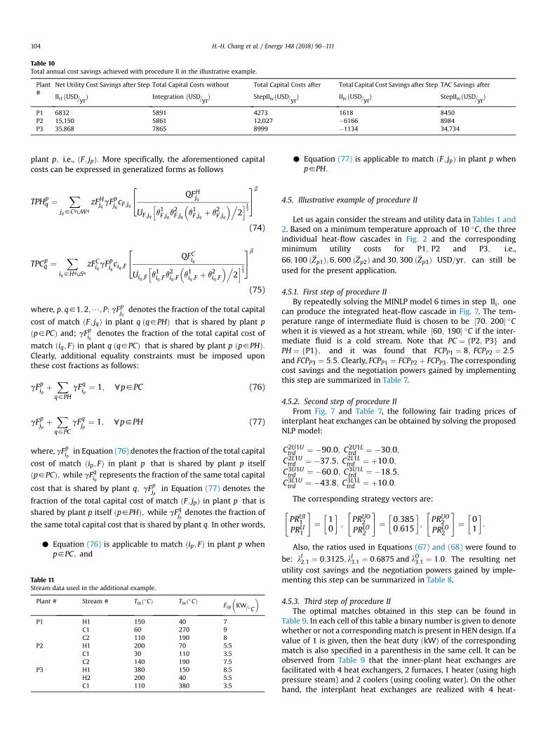
Table 10Total annual cost savings achieved with procedure II in the illustrative example.

Plant#

Net Utility Cost Savings after Step

IIi1�USD=yr

� Total Capital Costs without


� Total Capital Costs after

StepIIiv�USD=yr

� Total Capital Cost Savings after Step

IIiv�USD=yr

� TAC Savings after

StepIIiv�USD=yr

�P1 6832 5891 4273 1618 8450P2 15,150 5861 12,027 �6166 8984P3 35,868 7865 8999 �1134 34,734


plant p; i.e., ðF; jpÞ: More specifically, the aforementioned capitalcosts can be expressed in generalized forms as follows

TPHpq ¼

Xjq2Cq∪Wq

zFHjq gFpjqcF;jq

24 QFHjq

UF;jq

hq1F;jqq

2F;jq

�q1F;jq þ q2F;jq

�.2i13

35b

(74)

TPCpq ¼

Xiq2Hq∪Sq

zFCiqgFpiqciq;F

24 QFCiq

Uiq;F

hq1iq;Fq

2iq;F

�q1iq;F þ q2iq;F

�.2i13

35b

(75)

where, p; q21;2;/; P; gFpjq denotes the fraction of the total capital

cost of match ðF; jqÞ in plant q ðq2PHÞ that is shared by plant p

ðp2PCÞ and; gFpiq denotes the fraction of the total capital cost of

match ðiq; FÞ in plant q ðq2PCÞ that is shared by plant p ðp2PHÞ:Clearly, additional equality constraints must be imposed uponthese cost fractions as follows:

gFpip þXq2PH

gFqip ¼ 1; cp2PC (76)

gFpjp þXq2PC

gFqjp ¼ 1; cp2PH (77)

where, gFpip in Equation (76) denotes the fraction of the total capital

cost of match ðip; FÞ in plant p that is shared by plant p itselfðp2PCÞ; while gFqip represents the fraction of the same total capital

cost that is shared by plant q; gFpjp in Equation (77) denotes the

fraction of the total capital cost of match ðF; jpÞ in plant p that isshared by plant p itself ðp2PHÞ; while gFqjp denotes the fraction of

the same total capital cost that is shared by plant q: In other words,

C Equation (76) is applicable to match ðip; FÞ in plant p whenp2PC; and

Table 11Stream data used in the additional example.

Plant # Stream # Tinð�CÞ Tinð�CÞ Fcp

�KW=�C

�

P1 H1 150 40 7C1 60 270 9C2 110 190 8

P2 H1 200 70 5.5C1 30 110 3.5C2 140 190 7.5

P3 H1 380 150 8.5H2 200 40 5.5C1 110 380 3.5

C Equation (77) is applicable to match ðF; jpÞ in plant p whenp2PH:

4.5. Illustrative example of procedure II

Let us again consider the stream and utility data in Tables 1 and2. Based on a minimum temperature approach of  10 �C, the threeindividual heat-flow cascades in Fig. 2 and the correspondingminimum utility costs for P1; P2 and P3; i.e.,66;100 ðZp1Þ;6;600 ðZp2Þ and 30;300 ðZp3Þ USD=yr; can still beused for the present application.

4.5.1. First step of procedure IIBy repeatedly solving the MINLP model 6 times in step  IIi; one

can produce the integrated heat-flow cascade in Fig. 7. The tem-perature range of intermediate fluid is chosen to be  ½70; 200� �Cwhen it is viewed as a hot stream, while  ½60; 190� �C if the inter-mediate fluid is a cold stream. Note that PC ¼ fP2;  P3g andPH ¼ fP1g; and it was found that FCPP1 ¼ 8; FCPP2 ¼ 2:5and FCPP3 ¼ 5:5: Clearly, FCPP1 ¼ FCPP2 þ FCPP3: The correspondingcost savings and the negotiation powers gained by implementingthis step are summarized in Table 7.

4.5.2. Second step of procedure IIFrom Fig. 7 and Table 7, the following fair trading prices of

interplant heat exchanges can be obtained by solving the proposedNLP model:

C2U1Utrd ¼ �90:0; C2U1L

trd ¼ �30:0;C2L1Utrd ¼ �37:5; C2L1L

trd ¼ þ10:0;C3U1Utrd ¼ �60:0; C3U1L

trd ¼ �18:5;C3L1Utrd ¼ �43:8; C3L1L

trd ¼ þ10:0:

The corresponding strategy vectors are:"PRUI1PRLI1

#¼10

;

"PRUO2PRLO2

#¼0:3850:615

;

"PRUO2PRLO2

#¼01

:

Also, the ratios used in Equations (67) and (68) were found to

be: lI2;1 ¼ 0:3125; lI3;1 ¼ 0:6875 and lO3;1 ¼ 1:0: The resulting netutility cost savings and the negotiation powers gained by imple-menting this step can be summarized in Table 8.

4.5.3. Third step of procedure IIThe optimal matches obtained in this step can be found in

Table 9. In each cell of this table a binary number is given to denotewhether or not a correspondingmatch is present in HEN design. If avalue of 1 is given, then the heat duty ðkWÞ of the correspondingmatch is also specified in a parenthesis in the same cell. It can beobserved from Table 9 that the inner-plant heat exchanges arefacilitated with 4 heat exchangers, 2 furnaces, 1 heater (using highpressure steam) and 2 coolers (using cooling water). On the otherhand, the interplant heat exchanges are realized with 4 heat-

Table 12Utility data used in the additional example.

Plant # Utility Type Temperature ð�CÞUnit Cost

�USD=KW$yr

� Upper Limit ðKWÞ

P1 Cooling water 25 10 5000High p. steam 400 70 5000Medium p. steam 280 50 5000Low p. steam 200 40 5000

P2 Cooling water 25 22.5 5000High p. steam 400 60 5000Medium p. steam 280 40 5000Low p. steam 200 25 5000

P3 Cooling water 25 30 5000High p. steam 400 80 5000Medium p. steam 280 35 5000Low p. steam 200 30 5000

Fig. 9. Standalone heat-flow cascades in the additional example.


transfer units. The intermediate fluid is used as the cold stream inone such unit in plant P2 and also in another in plant P3, while it isthe hot stream in two separate units in plant P1.

4.5.4. Fourth step of procedure IIOn the basis the optimal matches listed in Table 9, a unique

superstructure can be built for every process stream in the threeplants under consideration. The objective function defined byEquations (37), (39), (41) and (72)e(75) can then be establishedaccording to the negotiation powers given in Table 8, while theother model constraints can be obtained by applying the basicprinciples of material and energy balances to the superstructures[3]. The annualization factor in Equation (73), i.e., Af ; was also set at0.1349. All cost coefficients in Equations (41), (74) and (75) werechosen to be 670 USD=m1:66 and b ¼ 0:83; while all overall heat-

transfer coefficients were taken to be 1 W=m2$K: Finally, the tem-perature rise of cooling water in every cooler was set to be 5 �C.

By solving the corresponding NLP program, one could generatethe interplant HEN design presented in Fig. 8 and the final eco-nomic assessment in Table 10. It can be observed that, although thecapital investments of plants P2 and P3must be increased to realizethe required inner- and inter-plant heat exchanges, this interplantheat integration project should still be quite feasible since the TACsavings of all plants are positive and reasonably distributed.

5. Case studies

By comparing the net savings in utility costs (see Tables 4 and 8)achieved in the aforementioned examples and those reportedpreviously in Cheng et al. [6], i.e.,  74;450 USD=yr; one could

Fig. 10. Integrated heat-flow cascades built at the first step of procedure I in the additional example.

Fig. 11. Interplant HEN design produced with procedure I in the additional example.

Table 13Total annual cost savings achieved with procedure I in the additional example.

Plant#


Iii�USD=yr



� Total Capital Costs after Step

Iiv�USD=yr

� Total Capital Cost Savings after

Step Iiv�USD=yr


Iiv�USD=yr

�P1 9748 6066 8367 �2500 7248P2 38,783 6321 8152 �1882 36,901P3 25,219 4533 6674 �1363 23,856


conclude that in general the overall energy cost of a direct heatintegration scheme should be lower than any of its indirect coun-terpart and, also, the sum of net utility cost savings achieved withan intermediate fluid should be larger than that with the heatingand cooling utilities. From Figs. 2 and 3, it can be observed that theminimum consumption rates of steams and cooling water of thestandalone plants are basically the same as those of the utility-facilitated indirect heat integration scheme. Since every availablehot/cold utility in the latter case is essentially a common heatsource/sink shared by all plants, the total utility cost saving re-ported in Table 3, i.e.,55;400 ð¼ 55;700� 20;400þ 20;100Þ USD=yr; is achieved in stepIi simply by replacing the utilities used in standalone cascades(Fig. 2) with their cheapest alternatives (Fig. 3). One can also seefrom Figs. 3 and 7 that, instead of sharing utilities across the plantboundaries, the indirect interplant heat integration scheme can bemade more efficient by using an intermediate fluid to providebetter heat-exchange opportunities. Furthermore, from Figs. 7 and3 in Cheng et al. [6], one would expect that a direct interplant heatintegration scheme can be adopted to reap the largest possibleenergy saving as long as the required interplant heat exchanges arerealizable in practice. Finally, in the illustrative example discussed

Fig. 12. Integrated heat-flow cascades built at the firs

above, the total capital cost of the HEN synthesized with procedureI is lower than that with procedure II and, also, the former isstructurally simpler and should be considered as a more operableand controllable design.

An extra example is presented below to further confirm theabove findings:

5.1. Process data

Tables 11 and 12 respectively show the stream and utility dataused in an additional example. Based on a minimum temperatureapproach of  10 K, the corresponding standalone heat-flow cas-cades can be built and they are given in Fig. 9. The minimum utilitycosts of P1, P2 and P3 can be determined respectively to be88;100 ðZp1Þ;30;100 ðZp2Þ; and 60;500 ðZp3Þ;USD=yr.

5.2. Procedure I

The integrated heat-flow cascade given in Fig. 10 was producedat the first step of procedure I. Although the required utility con-sumption rates are the same as those in the standalone heat-flowcascades (see Fig. 9), the cheapest utility is adopted at every

t step of procedure II in the additional example.

Fig. 13. Interplant HEN design produced with procedure II in the additional example.


occasion in this integrated scheme, i.e., the cooling water is alwaystaken from P1, the high- and low-pressure steams are from P2, andthe medium-pressure steam is from P3. The resulting interplantHEN design is presented in Fig. 11, while a complete economicsummary is provided in Table 13.

5.3. Procedure II

The integrated heat-flow cascade in Fig. 12 was produced byapplying the first step of procedure II. The temperature range of hotoil in this case can be chosen to be  ½70; 280� �C if it is used as a hot

Table 14Total annual cost savings achieved with procedure II in the additional example.

Plant#


IIi1�USD=yr



� Total Cap

StepIIiv�U

P1 73,208 6066 11,841P2 6965 6321 7096P3 36,237 4533 4691

stream, while  ½60; 270� �C if otherwise. Note that PC ¼ fP2;  P3gand PH ¼ fP1g; and it was determined thatFCPP1 ¼ 9; FCPP2 ¼ 0;619 and FCPP3 ¼ 8:381: Note that, by usingthe intermediate fluid, a significant amount of 1459:5 kW can bereduced respectively from the hot and cold utility consumptionrates of the integrated scheme obtained with procedure I (seeFigs. 10 and 12). By adopting the same parameter values presentedpreviously in subsection 3.5.4 or 4.5.4, one can produce the inter-plant HEN design in Fig. 13 and the corresponding cost summarycan be found in Table 14.

ital Costs after

SD=yr� Total Capital Cost Savings after

Step Iiv�USD=yr


IIiv�USD=yr

�

�5775 67,433�775 6190�158 36,079


5.4. Cost analysis

From Tables 13 and 14, it can be observed that these optimiza-tion results clearly reaffirm the conclusions drawn from the pre-vious example (see the beginning of Section 5). Notice that the totalutility cost saving achieved with the heating and cooling utilitiesð73;750 USD=yrÞ is much smaller than that with the intermediatefluid ð116;410 USD=yrÞ: This difference is probably due to theirroles in facilitating heat flows between plants. Although various hotand cold utilities may be available in different plants, they are allsupposed to be treated equally without distinguishing their origins.Thus, if the interplant heat exchanges are facilitated with utilities,then the total hot and cold utility consumption rates in every plantshould respectively remain unchanged. A considerable utility costsaving may still be achievable in this scenario due to the use ofcheaper alternatives. On the other hand, notice that the interme-diate fluid is treated as either an extra hot or cold process stream inevery individual plant. These additional streams are selected in stepIIi for optimally adjusting the grand composite curve of each plantso as to make the corresponding total utility cost lower than that ofthe standalone counterpart. As a result, the overall consumptionrates of hot and cold utilities of the entire site can both be reducedto lower levels as well.

However, since the intermediate fluid is present in a muchwider temperature range than that of any hot or cold utility, theinterplant HEN design synthesized with the intermediate fluid re-quires a slightly higher total capital cost than the utility-facilitateddesign. This tendency is also consistent with that found in theprevious example. Finally, note that the eventual feasibility of eachinterplant heat integration program can also be ensured by thereasonably distributed TAC savings among all participatingmembers.

6. Conclusions

This study aims to improve the practical applicability of inter-plant heat integration scheme. An existing game-theory basedsequential optimization strategy [6] has been improved in thiswork on the basis of the individual negotiation power of everyparticipating plant to stipulate the “fair” price for each energytrade, to determine the “reasonable” proportions of capital cost tobe shouldered by the involved parties of every interplant heatexchanger, and to produce an acceptable distribution of TAC sav-ings. Also, to address various safety and operational concernsagainst direct heat transfers across plant boundaries, the interplantheat flows have been facilitated in the proposed integrationschemes with either the available utilities or an extra intermediatefluid. Because of these additional practical features in interplantheat integration, realization of the resulting financial and envi-ronmental benefits should become more likely. Furthermore, fromthe optimization results obtained in case studies, one can find thatfeasible schemes can indeed be synthesized with the above twoprocedures. The interplant HEN design generated with procedure Ishould be simpler andmore operable, while its counterpart createdby procedure II is usually more energy efficient.

Nomenclature

AbbreviationsHEN heat exchanger networkLP linear programMILP mixed-integer linear programMINLP mixed-integer nonlinear programmingNA the corresponding heat transfer is not allowed

NLP nonlinear programmingTAC total annual costTSHI total site heat integration

SetsCpk the set of cold streams in interval k of plant p

Cp the set of cold streams in plant p

EUp the set of temperature intervals above the pinch in plantp

ELp the set of temperature intervals below the pinch in plantp

Hpk the set of hot process streams in interval k of plant p

Hp the set of hot process streams in plant p~Hpk the set of hot process streams in or above interval k of

plant pPC the set of plants in which the intermediate fluid is

treated as a cold streamPH the set of plants in which the intermediate fluid is

treated as a hot streamS the set of all hot utilitiesSp the set of hot utilities in plant pSpk the set of hot utilities in interval k of plant p~Spk the set of hot utilities in or above interval k of plant pW the set of all cold utilitiesWp the set of cold utilities in plant pWp

k the set of cold utilities in interval k of plant p

SuperscriptsH hot streamC cold streampUqiL from above the pinch in plant p to below the pinch in

plant qipUqiU from above the pinch in plant p to above the pinch in

plant qi

Indicesk label of temperature interval k ð k ¼ 1;2;/;KÞp label of plant pðq0 ¼ 1;2;/; PÞq label of plant qðq0 ¼ 1;2;/; PÞq0 label of plant q0ðq0 ¼ 1;2;/; PÞip label of hot process stream ip in plant p:jp label of cold process streamjp in plant p:mp label of hot utility mp in plant p:np label of cold utility np in plant p:

ParametersAf the annualization factorcip;jq the coefficient in the capital cost model of heat

exchanger between hot stream ip and cold stream jqðUSD=m1:66Þ

cip;jq0 the coefficient in the capital cost model of heat

exchanger between hot stream ip and cold stream jqðUSD=m1:66Þ

cF;jq the coefficient in the capital cost model of heatexchanger between intermediate fluid F and coldstream jq ðUSD=m1:66Þ

ciq;F the coefficient in the capital cost model of heatexchanger between hot stream iq and intermediate fluid

F ðUSD=m1:66Þ


CHUp the lowest unit cost of hot utility needed in plant p to

facilitate the corresponding interplant heat flowðUSD=kW$yÞ

CCUp the lowest unit cost of cold utility needed in plant p to

facilitate the corresponding interplant heat flowðUSD=kW$yÞ

cmp the unit cost of hot utility mp ðUSD=kW$yÞcnp the unit cost of cold utility np ðUSD=kW$yÞK the total number of temperature intervalsP the total number of plants taking part in the interplant

heat integration projectQHip;k

the heat released by hot stream ip in temperature

interval k ðkWÞQCjp;k

the heat absorbed by cold stream jp in temperature

interval k ðkWÞQSmp

the upper bound of the consumption rate of hot utilitymp ðkWÞ

QWnpthe upper bound of the consumption rate of cold utilitynp ðkWÞ

Uip;jq the overall heat transfer coefficient between hot stream

ip and cold stream jq ðkW=m2$KÞUip;jq0 the overall heat transfer coefficient between hot stream

ip and cold stream jq0 ðkW=m2$KÞUiq;jp the overall heat transfer coefficient between hot stream

iq and cold stream jp ðkW=m2$KÞUF;jq the overall heat transfer coefficient between hot oil F

and cold stream jp ðkW=m2$KÞUiq;F the overall heat transfer coefficient between hot oil F

and cold stream jp ðkW=m2$KÞDTmin the minimum temperature approach ð�CÞ

VariablesAp the payoff matrix of plant p ðp ¼ 1;2;/; PÞAp;qi a sub-matrix of the payoff values between plant p and

plant qiCpUqiUtrd the trade price paid by plant p for transferring a unit of

heat from a temperature above the pinch point of plantp to a temperature above the pinch point of plant qiðUSD=kW$yÞ

CpUqiLtrd the trade price paid by plant p for transferring a unit of

heat from a temperature above the pinch point of plantp to a temperature below the pinch point of plant qiðUSD=kW$yÞ

CpLqiUtrd the trade price paid by plant p for transferring a unit of

heat from a temperature below the pinch point of plantp to a temperature above the pinch point of plant qiðUSD=kW$yÞ

CpLqiUtrd the trade price paid by plant p for transferring a unit of

heat from a temperature below the pinch point ofplant p to a temperature below the pinch point of plantqi ðUSD=kW$yÞ

CqiUpUtrd the trade price paid by plant qi for transferring a unit of

heat from a temperature above the pinch point of plantqi to a temperature above the pinch point of plant pðUSD=kW$yÞ

CqiLpUtrd the trade price paid by plant qi for transferring a unit of

heat from a temperature below the pinch point of plant

qi to a temperature above the pinch point of plant pðUSD=kW$yÞ

CqiUpLtrd the trade price paid by plant qi for transferring a unit of

heat from a temperature above the pinch point of plantqi to a temperature below the pinch point of plant pðUSD=kW$yÞ

CqiLpLtrd the trade price paid by plant qi for transferring a unit of

heat from a temperature below the pinch point of plantqi to a temperature below the pinch point of plant pðUSD=kW$yÞ

CLIp the minimum total capital cost of a standalone HENdesign in plant p ðUSD=yÞ

Payoff pLqiL the unit payoff value of exporting heat at a temperaturebelow the pinch in plant p to a temperature below thepinch in plant qi ðUSD=kW$yÞ

Payoff qiUpU the unit payoff value of exporting heat at a temperatureabove the pinch in plant qi to a temperature above thepinch in plant p ðUSD=kW$yÞ

Payoff qiLpU the unit payoff value of exporting heat at a temperaturebelow the pinch in plant qi to a temperature above thepinch in plant p ðUSD=kW$yÞ

Payoff qiUpL the unit payoff value of exporting heat at a temperatureabove the pinch in plant qi to a temperature below thepinch in plant p ðUSD=kW$yÞ

Payoff qiLpL the unit payoff value of exporting heat at a temperaturebelow the pinch in plant qi to a temperature below thepinch in plant p ðUSD=kW$yÞ

pfp the total revenue received by plant p via energy tradesðUSD=yÞ

Qip;jp;k the amount of heat exchanged between hot stream ipand cold stream jp in interval k of plant p ðkWÞ

Qip;np;k the amount of heat exchanged between hot stream ipand cold utility np in interval k of plant p ðkWÞ

Qip;nq0 ;k the amount of heat exchanged between hot stream ip in

interval k and cold utility nq0 of plant q0 ðkWÞQmp;jp ;k the amount of heat exchanged between hot utility mp

and cold stream jp in interval k of plant p ðkWÞQmp;jq0 ;k the amount of heat exchanged between hot utilitymp in

interval k of plant p and cold stream jq0 of plant q0 ðkWÞQmq ;jp;k the amount of heat exchanged between hot utilitymq in

plant q and cold stream jp in interval k of plant p ðkWÞQEp the total volume of energy traffic in and out of plant p

ðkWÞQCUq;p

k the total heat-exchange rate between all hot streams ininterval k of plant q and all cold utilities in plant p ðkWÞ

QCUp;qk the total heat-exchange rate between all hot streams in

interval k of plant p and all cold utilities in plant q ðkWÞQFCip;k the amount of heat exchanged between hot stream ip

and hot oil in interval k of plant p ðkWÞQFCmp;k

the amount of heat exchanged between hot utility mp

and hot oil in interval k of plant p ðkWÞQFHjp;k the amount of heat exchanged between hot oil and cold

stream jp in interval k of plant p ðkWÞQFHnp;k

the amount of heat exchanged between hot oil and cold

utility np in interval k of plant p ðkWÞQHUq;p

k the total heat-exchange rate between all heatingutilities in plant q and all cold streams in interval k ofplant p ðkWÞ


QHUp;qk the total heat-exchange rate between all heating

utilities in plant p and all cold streams in interval k ofplant q ðkWÞ

QTCp;k the amount of heat absorbed by intermediate fluid as a

cold stream in interval k of plant p ðkWÞQTHp;k the amount of heat released by intermediate fluid as a

hot stream in interval k of plant p ðkWÞSUp the utility cost saving of plant p ðUSD=yÞSTp the total cost saving realized by plant p after inter-plant

heat integration ðUSD=yÞTCI

p the total capital cost of all inner-plant matches of plant pin an interplant heat integration scheme ðUSD=yÞ

TPCpp a fraction of the total capital cost of interplant matches

in plant p and each can be denoted as ðip; FÞ ðUSD=yÞTPHp

q a fraction of the total capital cost of interplant matchesin plant q and each is denoted as ðF; jqÞ ðUSD=yÞ

TRDp;q0 the capital cost of interplant match ðip; jq0 Þ shared byplant p ðUSD=yÞ

TRDq;p the capitasssssl cost of interplant match ðiq; jpÞ sharedby plant p ðUSD=yÞ

xp the strategy vector of plant p

Zp the minimum total utility cost of a standalone HEN inplant p ðUSD=yÞ

Z0p the minimum total utility cost of plant p achieved with

interplant heat integration ðUSD=yÞZip;jp the binary parameter to denote if the corresponding

matches between ip and jp are present in HENQSmp;k the consumption rate of hot utility mp of plant p in

temperature interval k ðkWÞQWnp;k the consumption rate of cold utility np of plant p in

temperature interval k ðkWÞRFk the heat residue fromhot oil in interval k of plant p ðkWÞRip;k the heat residue from hot process stream i in interval k

of plant p ðkWÞRmp;k the heat residue fromhot utilitym in interval k of plant p

ðkWÞgpip ;jq0

the proportions of capital cost shared by plant p for the

heat exchanger facilitating heat export from hot streamip to cold stream jq0 (dimensionless)

gq0

ip ;jq0 the proportions of capital cost shared by plant q

0for the

heat exchanger facilitating heat export from hot streamip to cold stream jq0 (dimensionless)

gpiq ;jp

the proportions of capital cost shared by plant p for the

exchanger facilitating heat import from hot streamiqtocold streamjp (dimensionless)

gqiq ;jp

the proportions of capital cost shared by plant q for the

exchanger facilitating heat import from hot stream iqtocold stream jp (dimensionless)

lOp;q0 the fraction of total heat exported by plant p that isreceived by plant q0

lIq;p the fraction of total heat imported by plant p that isreleased by plant q

gFpjq the fraction of the total capital cost of match ðF; jqÞ inplant q ðq2PHÞ that is shared by plant p ðp2PCÞ

gFpiq the fraction of the total capital cost of match ðiq; FÞ inplant q ðq2PCÞ that is shared by plant p ðp2PHÞ

References

[1] Yee TF, Grossmann IE. Simultaneous optimization models for heat integratione II. heat exchanger network synthesis. Comput Chem Eng 1990;14:1165e84.

[2] Papoulias SA, Grossmann IE. A structural optimization approach in processsynthesis e II. heat recovery networks. Comput Chem Eng 1983;7:707e21.

[3] Floudas CA, Ciric AR, Grossmann IE. Automatic synthesis of optimum heatexchanger network configurations. AIChE J 1986;32:276e90.

[4] Bagajewicz MJ, Rodera H. Multiple plant heat integration in a total site. AIChE J2002;48:2255e70.

[5] Kralj AK. Heat Integration between two biodiesel processes using a simplemethod. Energy Fuels 2008;22:1972e9.

[6] Liew PY, Theo WL, Alwi SRW, Lim JS, Manan ZA, Klemes JJ, Varbanov PS. TotalSite Heat Integration planning and design for industrial, urban and renewablesystems. Renew Sustain Energy Rev 2017;68:964e85.

[7] Hackl R, Harvey S. From heat integration targets toward implementation -ATSA (total site analysis)-based design approach for heat recovery systems inindustrial clusters. Energy 2015;90:163e72.

[8] Chang C, Chen X, Wang Y, Feng X. Simultaneous optimization of multi-plantheat integration using intermediate fluid circles. Energy 2017;121:306e17.

[9] Wang Y, Chang C, Feng X. A systematic framework for multi-plants heatintegration combining direct and indirect heat integration methods. Energy2015;90:56e67.

[10] Matsuda K, Hirochi Y, Tatsumi H, Shire T. Applying heat integration total sitebased pinch technology to a large industrial area in Japan to further improveperformance of highly efficient process plants. Energy 2009;34:1687e92.

[11] Liew PY, Alwi SR, Klemes JJ, Varbanov PS, Manan ZA. Algorithmic targeting forTotal Site Heat Integration with variable energy supply/demand. Appl ThermEng 2014;70:1073e83.

[12] Liew PY, Lim JS, Alwi SR, Manan ZA, Varbanov PS, Klemes JJ. A retrofitframework for Total Site heat recovery systems. Appl Energy 2014;135:778e90.

[13] Tarighaleslami AH, Walmsley TG, Atkins MJ, Walmsley MRW, Liew PY,Neale JR. A Unified Total Site Heat Integration targeting method for isothermaland non-isothermal utilities. Energy 2017;119:10e25.

[14] Zhang BJ, Li J, Zhang ZL, Wang K, Chen QL. Simultaneous design of heatexchanger network for heat integration using hot direct discharges/feedsbetween process plants. Energy 2016;109:400e11.

[15] Cheng SL, Chang CT, Jiang D. A game-theory based optimization strategy toconfigure inter-plant heat integration schemes. Chem Eng Sci 2014;118:60e73.

[16] Nash JF. Non-cooperative games. Ann Math 1951;54:286e95.[17] Hiete M, Ludwig J, Schultmann F. Intercompany energy integration - adap-

tation of thermal pinch analysis and allocation of savings. J Ind Ecol 2012;16:689e98.

[18] Chew IML, Tan R, Foo DCY, Chiu ASF. Game theory approach to the analysis ofinter-plant water integration in an eco-industrial park. J Clean Prod 2009;17:1611e9.

[19] Yue D, You F. Fair profit allocation in supply chain optimization with transferprice and revenue sharing: MINLP model and algorithm for cellulosic biofuelsupply chains. AIChE J 2014;60:3211e29.

[20] Torres AI, Stephanopoulos G. Design of multi-actor distributed processingsystems: a game-theoretical approach. AIChE J 2016;62:3369e91.

[21] Bandyopadhyay S, Varghese J, Bansal V. Targeting for cogeneration potentialthrough total site integration. Appl Therm Eng 2010;30:6e14.

[22] Quintas LG. A Note on polymatrix games. Int J Game Theor 1989;18:261e72.

http://refhub.elsevier.com/S0360-5442(18)30124-5/sref1













































































game-theory based optimization strategies for stepwise...

Documents