game theory basics - department of mathematics · game theory basics bernhard von stengel...
TRANSCRIPT

Game Theory Basics
Bernhard von Stengel
Department of Mathematics, London School of Economics,Houghton St, London WC2A 2AE, United Kingdom
email: [email protected]
February 15, 2011

ii
The material in this book has been adapted and developed from material originallyproduced for the BSc Mathematics and Economics by distance learning offered by theUniversity of London External Programme (www.londonexternal.ac.uk).
I am grateful to George Zouros for his valuable comments, and to Rahul Savani forhis continuing interest in this project, his thorough reading of earlier drafts, and the funwe have in joint research and writing on game theory.

Preface
Game theory is the formal study of conflict and cooperation. It is concerned with situa-tions where “players” interact, so that it matters to each player what the other players do.Game theory provides mathematical tools to model, structure and analyse such interac-tive scenarios. The players may be, for example, competing firms, political voters, matinganimals, or buyers and sellers on the internet. The language and concepts of game theoryare widely used in economics, political science, biology, and computer science, to namejust a few disciplines.
Game theory helps to understand effects of interaction that seem puzzling at first.For example, the famous “prisoners’ dilemma” explains why fishers can exhaust theirresources by over-fishing: they hurt themselves collectively, but each fisher on his owncannot really change this and still profits by fishing as much as possible. Other insightscome from the way of looking at interactive situations. Game theory treats players equallyand recommends to each player how to play well, given what the other players do. Thismindset is useful in strategic questions of management, because “you put yourself in youropponent’s shoes”.
Game theory is fascinating as a topic because of its diverse applications. The ideasof game theory started with mathematicians, most notably the outstanding mathematicianJohn von Neumann (1903–1957). In the 1950s, a group of young researchers in mathe-matics at Princeton developed game theory further, among them John Nash, Harold Kuhnand Lloyd Shapley, and these pioneers can still, over 50 years later, be met at conferenceson game theory. Most research in game theory is now done by economists and other socialscientists.
My own interests are in the mathematics of games, so I see my own research in thetradition of early game theory. My research specialty is the connection of game theoryto computer science. In particular, I develop methods to find equilibria of games, whichmake use of insights from geometry. That interest is partly reflected in the choice of topicsin this book. This book has also a strong emphasis on methods, so you will learn a lotof “tricks” that allow you to understand games quickly. With these methods at hand, youwill be in a position to analyse games that you can create for applications to managementor economics.
Structure of this book
Chapter 1 on combinatorial games is on playing and winning games with perfect informa-tion defined by rules, in particular a simple game called “nim”, which has a central role
iii

iv
in that theory. This chapter introduces abstract mathematics with a fun topic. You wouldprobably not learn its content otherwise, because it does not have a typical applicationin economics. However, every game theorist should know the basics of combinatorialgames. In fact, this can be seen as the motto for the contents of this book: what everygame theorist should know.
Chapter 1 on combinatorial games is independent of the other material. This topicis deliberately put at the beginning because it is more mathematical and formal than theother topics, so that it can be used to test whether you can cope with the abstract parts ofgame theory, and with the mathematical style of this subject.
Chapters 2, 3, and 4 successively build on each other. These chapters cover the mainconcepts and methods of non-cooperative game theory.
With the exception of imperfect information, the fundamentals of non-cooperativegame theory are laid out in chapter 2. This part of game theory provides ways to model indetail the agents in an interactive situation, their possible actions, and their incentives. Themodel is called a game and the agents are called players. There are two types of games,called game trees and games in strategic form. The game tree (also called the extensiveform of a game) describes in depth the actions that are available to the players, how theseevolve over time, and what the players know or do not know about the game. (Games withimperfect information are treated in chapter 4.) The players’ incentives are modelled bypayoffs that these players want to maximise, which is the sole guiding principle in non-cooperative game theory. In contrast, cooperative game theory studies, for example, howplayers should split their proceeds when they decide to cooperate, but leaves it open howthey enforce an agreement. (A simple example of this cooperative approach is explainedin chapter 5 on bargaining.)
Chapter 3 shows that in certain games it may be useful to leave your actions uncertain.A nice example is the football penalty kick, which serves as our introduction to zero-sumgames (see figure 3.11). The striker should not always kick into the same corner, norshould the goalkeeper always jump into the same corner, even if they are better at scoringor saving a penalty there. It is better to be unpredictable! Game theory tells the playershow to choose optimal probabilities for each of their available strategies, which are thenused to mix these strategies randomly. With the help of mixed strategies, every game hasan equilibrium. This is the central result of John Nash, who discovered the equilibriumconcept in 1950 for general games. For zero-sum games, this was already found earlier byJohn von Neumann. It is easier to prove for zero-sum games that they have an equilibriumthan for general games. In a logical progression of topics, in particular when starting fromwin/lose games like nim, we could have treated zero-sum games before general games.However, we choose to treat zero-sum games later, as special cases of general games,because the latter are much more important in economics. In a course on game theory, onecould omit zero-sum games and their special properties, which is why we treat them in thelast section of chapter 3. However, one could not omit the concept of Nash equilibrium,which is therefore given prominence early on.
Chapter 4 explains how to model the information that players have in a game. Thisis done by means of so-called information sets in game trees, introduced in 1953 byHarold Kuhn. The central result of this chapter is called Kuhn’s theorem. Essentially, thisresult states that players can choose a “behaviour strategy”, which is a way of playing
v
the game that is not too complicated, provided they do not forget what they knew anddid earlier. This result is typically considered as technical, and given short shrift in manygame theory texts. We go into great detail in explaining this result. The first reason isthat it is a beautiful result of discrete mathematics, because elementary concepts like thegame tree and the information sets are combined naturally to give a new result. Secondly,the result is used in other, more elaborate “dynamic” games that develop over time. Formore advanced studies of game theory, it is therefore useful to have a solid understandingof game trees with imperfect information.
The final chapter 5 on bargaining is a particularly interesting application of non-cooperative theory. It is partly independent of chapters 3 and 4, so to a large extent itcan be understood after chapter 2. A first model provides conditions – called axioms –that an acceptable “solution” to bargaining situations should fulfil, and shows that theseaxioms lead to a unique solution of this kind. A second model of “alternating offers” ismore detailed and uses, in particular, the analysis of game trees with perfect informationintroduced in chapter 2. The “bargaining solution” is thereby given an incentive-basedjustification with a more detailed non-cooperative model.
Game theory, and this text, use only a few prerequisites from elementary linear alge-bra, probability theory, and some analysis. You should know that vectors and points havea geometric interpretation (for example, as either points or vectors in three-dimensionalspace if the dimension is three). It should be clear how to multiply matrices, and how tomultiply a matrix with a vector. The required notions from probability theory are that ofexpected value of a function (that is, function values weighted with their probabilities),and that independent events have a probability that is the product of the probabilities ofthe individual events. The concepts from analysis are those of a continuous function,which, for example, assumes its maximum on a compact (closed and bounded) domain.None of these concepts is difficult, and you are reminded of their basic ideas in the textwhenever they are needed.
We introduce and illustrate each concept with examples, many pictures, and a mini-mum of notation. Not every concept is defined with a formal definition (although manyconcepts are), but instead explained by means of an example. It should in each casebe clear how the concept applies in similar settings, and in general. On the other hand,this requires some maturity in dealing with mathematical concepts, and in being able togeneralise from examples.
Distinction to other textbooks
Game theory has seen an explosion in interest in recent years. Correspondingly, many newtextbooks on game theory have recently appeared. The present text is complementary (or“orthogonal”) to most existing textbooks.
First of all, it is mathematical in spirit, meaning it can be used as a textbook forteaching game theory as a mathematics course. On the other hand, the mathematics inthis book should be accessible enough to students of economics, management, and othersocial sciences.
vi
The book is relatively swift in treating games in strategic form and game trees in asingle chapter (chapter 3), which are often considered separately. I find these conceptssimple enough to allow for that approach.
Mixed strategies and the best response condition are very useful for finding equilibriain games, so they are given detailed treatment. Similarly, game trees with imperfect infor-mation, and the concepts of perfect recall and behaviour strategies, and Kuhn’s theorem,are also given an in-depth treatment, because this not found in many textbooks at thislevel.
The book does not try to be comprehensive in presenting the most relevant economicapplications of game theory. Corresponding “stories” are only told for illustration of theconcepts.
One book served as a starting point for the selection of the material, namely• K. Binmore, Fun and Games, D. C. Heath, 1991. Its recent, significantly revised
version is Playing for Real, Oxford University Press, 2007.This book describes nim as a game that one can learn to play perfectly. In turn, this
led me to the question of why the binary system has such an important role, and towardsthe study of combinatorial games. The topic of bargaining is also motivated by Binmore’sbook. At the same time, the present text is very different from Binmore’s book, becauseit tries to treat as few side topics as possible.
Two short sections can be considered as slightly non-standard side topics, namely thesections 2.9, Symmetries involving strategies, and 4.9 Perfect recall and order of moves,both marked with a star as “can be skipped at first reading”. I included them as topicsthat I have not found elsewhere. Section 4.9 demonstrates how to reason carefully aboutmoves in extensive games, and should help understand the perfect recall condition.
Methods, not philosophyThe general emphasis of the book is to teach methods, not philosophy. Game theoriststend to question and to justify the approaches they take, for example the concept of Nashequilibrium, and the assumed common knowledge of all players about the rules of thegame. These questions are of course very important. In fact, in practice these are probablythe very issues that make a game-theoretic analysis questionable. However, this problemis not remedied by a lengthy discussion of why one should play Nash equilibrium.
I think a student who learns about game theory should first become fluent in knowingthe modelling tools (such as game trees and the strategic form) and in analysing games(finding their Nash equilibria). That toolbox will then be useful when comparing differentgame-theoretic models and looking at their implications. In many disciplines that arefurther away from mathematics, these possible implications are typically more interestingthan the mathematical model itself (the model is necessarily imperfect, so there is no pointin being dogmatic about the analysis).
Contents
1 Nim and combinatorial games 11.1 Aims of the chapter . . . . . . . . . . . . . . . . . . . . . . . . . . . . . 11.2 Learning objectives . . . . . . . . . . . . . . . . . . . . . . . . . . . . . 11.3 Further reading . . . . . . . . . . . . . . . . . . . . . . . . . . . . . . . 21.4 What is combinatorial game theory? . . . . . . . . . . . . . . . . . . . . 21.5 Nim – rules . . . . . . . . . . . . . . . . . . . . . . . . . . . . . . . . . 41.6 Combinatorial games, in particular impartial games . . . . . . . . . . . . 51.7 Simpler games and notation for nim heaps . . . . . . . . . . . . . . . . . 61.8 Sums of games . . . . . . . . . . . . . . . . . . . . . . . . . . . . . . . 71.9 Equivalent games . . . . . . . . . . . . . . . . . . . . . . . . . . . . . . 91.10 Sums of nim heaps . . . . . . . . . . . . . . . . . . . . . . . . . . . . . 121.11 Poker nim and the mex rule . . . . . . . . . . . . . . . . . . . . . . . . . 161.12 Finding nim values . . . . . . . . . . . . . . . . . . . . . . . . . . . . . 171.13 Exercises for chapter 1 . . . . . . . . . . . . . . . . . . . . . . . . . . . 20
2 Games as trees and in strategic form 272.1 Learning objectives . . . . . . . . . . . . . . . . . . . . . . . . . . . . . 272.2 Further reading . . . . . . . . . . . . . . . . . . . . . . . . . . . . . . . 272.3 Introduction . . . . . . . . . . . . . . . . . . . . . . . . . . . . . . . . . 282.4 Definition of game trees . . . . . . . . . . . . . . . . . . . . . . . . . . . 282.5 Backward induction . . . . . . . . . . . . . . . . . . . . . . . . . . . . . 312.6 Strategies and strategy profiles . . . . . . . . . . . . . . . . . . . . . . . 322.7 Games in strategic form . . . . . . . . . . . . . . . . . . . . . . . . . . . 332.8 Symmetric games . . . . . . . . . . . . . . . . . . . . . . . . . . . . . . 342.9 Symmetries involving strategies∗ . . . . . . . . . . . . . . . . . . . . . . 372.10 Dominance and elimination of dominated strategies . . . . . . . . . . . . 382.11 Nash equilibrium . . . . . . . . . . . . . . . . . . . . . . . . . . . . . . 412.12 Reduced strategies . . . . . . . . . . . . . . . . . . . . . . . . . . . . . 432.13 Subgame perfect Nash equilibrium (SPNE) . . . . . . . . . . . . . . . . 452.14 Commitment games . . . . . . . . . . . . . . . . . . . . . . . . . . . . . 482.15 Exercises for chapter 2 . . . . . . . . . . . . . . . . . . . . . . . . . . . 52
3 Mixed strategy equilibria 593.1 Learning objectives . . . . . . . . . . . . . . . . . . . . . . . . . . . . . 593.2 Further reading . . . . . . . . . . . . . . . . . . . . . . . . . . . . . . . 59
vii

viii CONTENTS
3.3 Introduction . . . . . . . . . . . . . . . . . . . . . . . . . . . . . . . . . 603.4 Expected-utility payoffs . . . . . . . . . . . . . . . . . . . . . . . . . . . 613.5 Example: Compliance inspections . . . . . . . . . . . . . . . . . . . . . 623.6 Bimatrix games . . . . . . . . . . . . . . . . . . . . . . . . . . . . . . . 653.7 Matrix notation for expected payoffs . . . . . . . . . . . . . . . . . . . . 663.8 Convex combinations and mixed strategy sets . . . . . . . . . . . . . . . 683.9 The best response condition . . . . . . . . . . . . . . . . . . . . . . . . . 693.10 Existence of mixed equilibria . . . . . . . . . . . . . . . . . . . . . . . . 713.11 Finding mixed equilibria . . . . . . . . . . . . . . . . . . . . . . . . . . 733.12 The upper envelope method . . . . . . . . . . . . . . . . . . . . . . . . . 773.13 Degenerate games . . . . . . . . . . . . . . . . . . . . . . . . . . . . . . 803.14 Zero-sum games . . . . . . . . . . . . . . . . . . . . . . . . . . . . . . . 853.15 Exercises for chapter 3 . . . . . . . . . . . . . . . . . . . . . . . . . . . 91
4 Game trees with imperfect information 954.1 Learning objectives . . . . . . . . . . . . . . . . . . . . . . . . . . . . . 954.2 Further reading . . . . . . . . . . . . . . . . . . . . . . . . . . . . . . . 954.3 Introduction . . . . . . . . . . . . . . . . . . . . . . . . . . . . . . . . . 964.4 Information sets . . . . . . . . . . . . . . . . . . . . . . . . . . . . . . . 964.5 Extensive games . . . . . . . . . . . . . . . . . . . . . . . . . . . . . . 1024.6 Strategies for extensive games and the strategic form . . . . . . . . . . . 1044.7 Reduced strategies . . . . . . . . . . . . . . . . . . . . . . . . . . . . . 1054.8 Perfect recall . . . . . . . . . . . . . . . . . . . . . . . . . . . . . . . . 1064.9 Perfect recall and order of moves∗ . . . . . . . . . . . . . . . . . . . . . 1104.10 Behaviour strategies . . . . . . . . . . . . . . . . . . . . . . . . . . . . . 1124.11 Kuhn’s theorem: behaviour strategies suffice . . . . . . . . . . . . . . . . 1164.12 Subgames and subgame perfect equilibria . . . . . . . . . . . . . . . . . 1204.13 Exercises for chapter 4 . . . . . . . . . . . . . . . . . . . . . . . . . . . 122
5 Bargaining 1255.1 Learning objectives . . . . . . . . . . . . . . . . . . . . . . . . . . . . . 1255.2 Further reading . . . . . . . . . . . . . . . . . . . . . . . . . . . . . . . 1255.3 Introduction . . . . . . . . . . . . . . . . . . . . . . . . . . . . . . . . . 1255.4 Bargaining sets . . . . . . . . . . . . . . . . . . . . . . . . . . . . . . . 1265.5 Bargaining axioms . . . . . . . . . . . . . . . . . . . . . . . . . . . . . 1285.6 The Nash bargaining solution . . . . . . . . . . . . . . . . . . . . . . . . 1305.7 Splitting a unit pie . . . . . . . . . . . . . . . . . . . . . . . . . . . . . . 1345.8 The ultimatum game . . . . . . . . . . . . . . . . . . . . . . . . . . . . 1365.9 Alternating offers over two rounds . . . . . . . . . . . . . . . . . . . . . 1395.10 Alternating offers over several rounds . . . . . . . . . . . . . . . . . . . 1435.11 Stationary strategies . . . . . . . . . . . . . . . . . . . . . . . . . . . . . 1465.12 The Nash bargaining solution via alternating offers . . . . . . . . . . . . 1505.13 Exercises for chapter 5 . . . . . . . . . . . . . . . . . . . . . . . . . . . 151

CONTENTS ix
6 Geometric representation of equilibria 1556.1 Learning objectives . . . . . . . . . . . . . . . . . . . . . . . . . . . . . 1556.2 Further reading . . . . . . . . . . . . . . . . . . . . . . . . . . . . . . . 1556.3 Introduction . . . . . . . . . . . . . . . . . . . . . . . . . . . . . . . . . 1566.4 Best response regions . . . . . . . . . . . . . . . . . . . . . . . . . . . . 1566.5 Identifying equilibria . . . . . . . . . . . . . . . . . . . . . . . . . . . . 1626.6 The Lemke–Howson algorithm . . . . . . . . . . . . . . . . . . . . . . 1636.7 Odd number of Nash equilibria . . . . . . . . . . . . . . . . . . . . . . . 1666.8 Exercises for chapter 6 . . . . . . . . . . . . . . . . . . . . . . . . . . . 168
7 Linear programming and zero-sum games 1717.1 Learning objectives . . . . . . . . . . . . . . . . . . . . . . . . . . . . . 1717.2 Further reading . . . . . . . . . . . . . . . . . . . . . . . . . . . . . . . 1727.3 Linear programs and duality . . . . . . . . . . . . . . . . . . . . . . . . 1727.4 The minimax theorem via LP duality . . . . . . . . . . . . . . . . . . . . 1757.5 General LP duality . . . . . . . . . . . . . . . . . . . . . . . . . . . . . 1777.6 The Lemma of Farkas and proof of strong LP duality∗ . . . . . . . . . . . 1817.7 Exercises for chapter 7 . . . . . . . . . . . . . . . . . . . . . . . . . . . 185

x CONTENTS

Chapter 1
Nim and combinatorial games
1.1 Aims of the chapter
This chapter introduces the basics of combinatorial games, and explains the central roleof the game nim. A detailed summary of the chapter is given in section 1.4.
Furthermore, this chapter demonstrates the use of abstract mathematics in game the-ory. This chapter is written more formally than the other chapters, in parts in the tra-ditional mathematical style of definitions, theorems and proofs. One reason for doingthis, and why we start with combinatorial games, is that this topic and style serves as awarning shot to those who think that game theory, and this text in particular, is “easy”.If we started with the well-known “prisoner’s dilemma” (which makes its due appear-ance in Chapter 2), the less formally inclined student might be lulled into a false sense offamiliarity and “understanding”. We therefore start deliberately with an unfamiliar topic.
This is a mathematics text, with great emphasis on rigour and clarity, and on usingmathematical notions precisely. As mathematical prerequisites, game theory requires onlythe very basics of linear algebra, calculus and probability theory. However, game theoryprovides its own conceptual tools that are used to model and analyse interactive situa-tions. This text emphasises the mathematical structure of these concepts, which belong to“discrete mathematics”. Learning a number of new mathematical concepts is exemplifiedby combinatorial game theory, and it will continue in the study of classical game theoryin the later chapters.
1.2 Learning objectives
After studying this chapter, you should be able to:
• play nim optimally;
• explain the concepts of game-sums, equivalent games, nim values and the mex rule;
• apply these concepts to play other impartial games like those described in the exer-cises.
1
2 CHAPTER 1. NIM AND COMBINATORIAL GAMES
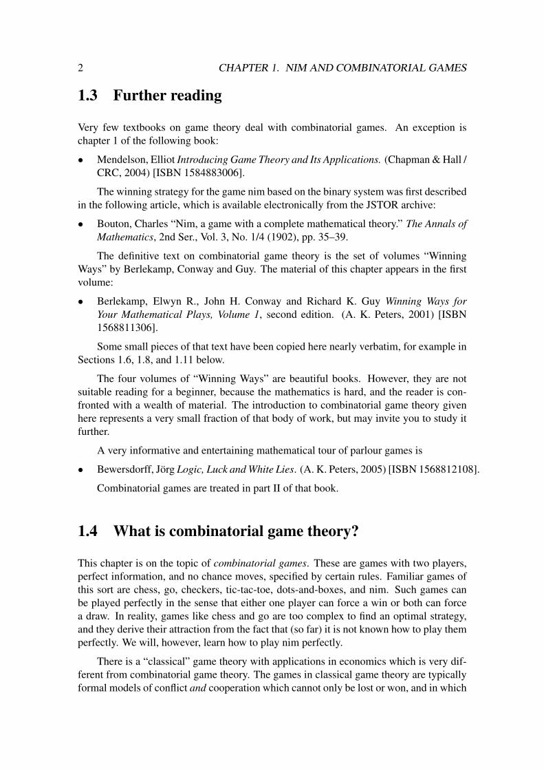
1.3 Further reading
Very few textbooks on game theory deal with combinatorial games. An exception ischapter 1 of the following book:
• Mendelson, Elliot Introducing Game Theory and Its Applications. (Chapman & Hall /CRC, 2004) [ISBN 1584883006].
The winning strategy for the game nim based on the binary system was first describedin the following article, which is available electronically from the JSTOR archive:
• Bouton, Charles “Nim, a game with a complete mathematical theory.” The Annals ofMathematics, 2nd Ser., Vol. 3, No. 1/4 (1902), pp. 35–39.
The definitive text on combinatorial game theory is the set of volumes “WinningWays” by Berlekamp, Conway and Guy. The material of this chapter appears in the firstvolume:
• Berlekamp, Elwyn R., John H. Conway and Richard K. Guy Winning Ways forYour Mathematical Plays, Volume 1, second edition. (A. K. Peters, 2001) [ISBN1568811306].
Some small pieces of that text have been copied here nearly verbatim, for example inSections 1.6, 1.8, and 1.11 below.
The four volumes of “Winning Ways” are beautiful books. However, they are notsuitable reading for a beginner, because the mathematics is hard, and the reader is con-fronted with a wealth of material. The introduction to combinatorial game theory givenhere represents a very small fraction of that body of work, but may invite you to study itfurther.
A very informative and entertaining mathematical tour of parlour games is
• Bewersdorff, Jorg Logic, Luck and White Lies. (A. K. Peters, 2005) [ISBN 1568812108].
Combinatorial games are treated in part II of that book.
1.4 What is combinatorial game theory?
This chapter is on the topic of combinatorial games. These are games with two players,perfect information, and no chance moves, specified by certain rules. Familiar games ofthis sort are chess, go, checkers, tic-tac-toe, dots-and-boxes, and nim. Such games canbe played perfectly in the sense that either one player can force a win or both can forcea draw. In reality, games like chess and go are too complex to find an optimal strategy,and they derive their attraction from the fact that (so far) it is not known how to play themperfectly. We will, however, learn how to play nim perfectly.
There is a “classical” game theory with applications in economics which is very dif-ferent from combinatorial game theory. The games in classical game theory are typicallyformal models of conflict and cooperation which cannot only be lost or won, and in which

1.4. WHAT IS COMBINATORIAL GAME THEORY? 3
there is often no perfect information about past and future moves. To the economist, com-binatorial games are not very interesting. Chapters 2–5 of the book are concerned withclassical game theory.
Why, then, study combinatorial games at all in a text that is mostly about classicalgame theory, and which aims to provide an insight into the theory of games as used in eco-nomics? The reason is that combinatorial games have a rich and interesting mathematicaltheory. We will explain the basics of that theory, in particular the central role of the gamenim for impartial games. It is non-trivial mathematics, it is fun, and you, the student, willhave learned something that you would most likely not have learned otherwise.
The first “trick” from combinatorial game theory is how to win in the game nim, usingthe binary system. Historically, that winning strategy was discovered first (published byCharles Bouton in 1902). Only later did the central importance of nim, in what is knownas the Sprague–Grundy theory of impartial games, become apparent. It also revealedwhy the binary system is important (and not, say, the ternary system, where numbers arewritten in base three), and learning that is more satisfying than just learning how to use it.
In this chapter, we first define the game nim and more general classes of games withperfect information. These are games where every player knows exactly the state of thegame. We then define and study the concepts listed in the learning outcomes above, whichare the concepts of game-sums, equivalent games, nim values and the mex rule. It is bestto learn these concepts by following the chapter in detail. We give a brief summary here,which will make more sense, and should be re-consulted, after a first study of the chapter(so do not despair if you do not understand this summary).
Mathematically, any game is defined by other “games” that a player can reach in hisfirst move. These games are called the options of the game. This seemingly circulardefinition of a “game” is sound because the options are simpler games, which need fewermoves in total until they end. The definition is therefore not circular, but recursive, andthe mathematical tool to argue about such games is that of mathematical induction, whichwill be used extensively (it will also recur in chapter 2 as “backward induction” for gametrees). Here, it is very helpful to be familiar with mathematical induction for provingstatements about natural numbers.
We focus here on impartial games, where the available moves are the same no matterwhether player I or player II is the player to make a move. Games are “combined” bythe simple rule that a player can make a move in exactly one of the games, which definesa sum of these games. In a “losing game”, the first player to move loses (assuming, asalways, that both players play as well as they can). An impartial game added to itselfis always losing, because any move can be copied in the other game, so that the secondplayer always has a move left. This is known as the “copycat” principle (lemma 1.6). Animportant observation is that a losing game can be “added” (via the game-sum operation)to any game without changing the winning or losing properties of the original game.
In section 1.10, the central theorem 1.10 explains the winning strategy in nim. Theimportance of nim for impartial games is then developed in section 1.11 via the beautifulmex rule. After the comparatively hard work of the earlier sections, we almost instantlyobtain that any impartial game is equivalent to a nim heap (corollary 1.13).

4 CHAPTER 1. NIM AND COMBINATORIAL GAMES
At the end of the chapter, the sizes of these equivalent nim heaps (called nim values)are computed for some examples of impartial games. Many other examples are studied inthe exercises.
Our exposition is distinct from the classic text “Winning Ways” in the following re-spects: First, we only consider impartial games, even though many aspects carry over tomore general combinatorial games. Secondly, we use a precise definition of equivalentgames (see section 1.9), because a game where you are bound to lose against a smart op-ponent is not the same as a game where you have already lost. Two such games are merelyequivalent, and the notion of equivalent games is helpful in understanding the theory. Sothis text is much more restricted, but to some extent more precise than “Winning Ways”,which should help make this topic accessible and enjoyable.
1.5 Nim – rules
The game nim is played with heaps (or piles) of chips (or counters, beans, pebbles,matches). Players alternate in making a move, by removing some chips from one ofthe heaps (at least one chip, possibly the entire heap). The first player who cannot moveany more loses the game.
The players will be called, rather unimaginatively, player I and player II, with player Ito start the game.
For example, consider three heaps of size 1,1,2. What is a good move? Removingone of the chips from the heap with two chips will create the position 1,1,1, then player IImust move to 1,1, then player I to 1, and then player II takes the last chip and wins. Sothis is not a good opening move. The winning move is to remove all chips from the heapof size 2, to reach position 1,1, and then player I will win. Hence we call 1,1,2 a winningposition, and 1,1 a losing position.
When moving in a winning position, the player to move can win by playing well, bymoving to a losing position of the other player. In a losing position, the player to movewill lose no matter what move she chooses, if her opponent plays well. This means thatall moves from a losing position lead to a winning position of the opponent. In contrast,one needs only one good move from a winning position that goes to a losing position ofthe next player.
Another winning position consists of three nim heaps of sizes 1,1,1. Here all movesresult in the same position and player I always wins. In general, a player in a winningposition must play well by picking the right move. We assume that players play well,forcing a win if they can.
Suppose nim is played with only two heaps. If the two heaps have equal size, forexample in position 4,4, then the first player to move loses (so this is a losing position),because player II can always copy player I’s move by equalising the two heaps. If the twoheaps have different sizes, then player I can equalise them by removing an appropriatenumber of chips from the larger heap, putting player II in a losing position. The rule for2-heap nim is therefore:

1.6. COMBINATORIAL GAMES, IN PARTICULAR IMPARTIAL GAMES 5
Lemma 1.1 The nim position m,n is winning if and only if m 6= n, otherwise losing, forall m,n≥ 0.
This lemma applies also when m = 0 or n = 0, and thus includes the cases that one orboth heap sizes are zero (meaning only one heap or no heap at all).
With three or more heaps, nim becomes more difficult. For example, it is not imme-diately clear if, say, positions 1,4,5 or 2,3,6 are winning or losing positions.
⇒ At this point, you should try exercise 1.1(a) on page 20.
1.6 Combinatorial games, in particular impartial games
The games we study in this chapter have, like nim, the following properties:
1. There are just two players.
2. There are several, usually finitely many, positions, and sometimes a particular start-ing position.
3. There are clearly defined rules that specify the moves that either player can makefrom a given position to the possible new positions, which are called the options ofthat position.
4. The two players move alternately, in the game as a whole.
5. In the normal play convention a player unable to move loses.
6. The rules are such that play will always come to an end because some player will beunable to move. This is called the ending condition. So there can be no games whichare drawn by repetition of moves.
7. Both players know what is going on, so there is perfect information.
8. There are no chance moves such as rolling dice or shuffling cards.
9. The game is impartial, that is, the possible moves of a player only depend on theposition but not on the player.
As a negation of condition 5, there is also the misere play convention where a playerunable to move wins. In the surrealist (and unsettling) movie “Last year at Marienbad”by Alain Resnais from 1962, misere nim is played, several times, with rows of matchesof sizes 1,3,5,7. If you have a chance, try to watch that movie and spot when the otherplayer (not the guy who brought the matches) makes a mistake! Note that this is miserenim, not nim, but you will be able to find out how to play it once you know how to playnim. (For games other than nim, normal play and misere versions are typically not sosimilar.)
In contrast to condition 9, games where the available moves depend on the player (asin chess where one player can only move white pieces and the other only black pieces)are called partisan games. Much of combinatorial game theory is about partisan games,which we do not consider to keep matters simple.

6 CHAPTER 1. NIM AND COMBINATORIAL GAMES
Chess, and the somewhat simpler tic-tac-toe, also fail condition 6 because they mayend in a tie or draw. The card game poker does not have perfect information (as requiredin 7) and would lose all its interest if it had. The analysis of poker, although it is alsoa win-or-lose game, leads to the “classical” theory of zero-sum games (with imperfectinformation) that we will consider later. The board game backgammon is a game withperfect information but with chance moves (violating condition 8) because dice are rolled.
We will be relatively informal in style, but our notions are precise. In condition 3above, for example, the term option refers to a position that is reachable in one movefrom the current position; do not use “option” when you mean “move”. Similarly, wewill later use the term strategy to define a plan of moves, one for every position that canoccur in the game. Do not use “strategy” when you mean “move”. However, we will takesome liberty in identifying a game with its starting position when the rules of the gameare clear.
⇒ Try now exercises 1.2 and 1.3 starting on page 20.
1.7 Simpler games and notation for nim heaps
A game, like nim, is defined by its rules, and a particular starting position. Let G be such aparticular instance of nim, say with the starting position 1,1,2. Knowing the rules, we canidentify G with its starting position. Then the options of G are 1,2, and 1,1,1, and 1,1.Here, position 1,2 is obtained by removing either the first or the second heap with onechip only, which gives the same result. Positions 1,1,1 and 1,1 are obtained by makinga move in the heap of size two. It is useful to list the options systematically, consideringone heap to move in at a time, so as not to overlook any option.
Each of the options of G is the starting position of another instance of nim, definingone of the new games H, J, K, say. We can also say that G is defined by the moves tothese games H, J, K, and we call these games also the options of G (by identifying themwith their starting positions; recall that the term “option” has been defined in point 3 ofsection 1.6).
That is, we can define a game as follows: Either the game has no move, and theplayer to move loses, or a game is given by one or several possible moves to new games,in which the other player makes the initial move. In our example, G is defined by thepossible moves to H, J, or K. With this definition, the entire game is completely specifiedby listing the initial moves and what games they lead to, because all subsequent use of therules is encoded in those games.
This is a recursive definition because a “game” is defined in terms of “game” itself.We have to add the ending condition that states that every sequence of moves in a gamemust eventually end, to make sure that a game cannot go on indefinitely.
This recursive condition is similar to defining the set of natural numbers as follows:(a) 0 is a natural number; (b) if n is a natural number, then so is n+1; and (c) all naturalnumbers are obtained in this way, starting from 0. Condition (c) can be formalised by the

1.8. SUMS OF GAMES 7
principle of induction that says: if a property P(n) is true for n = 0, and if the propertyP(n) implies P(n+1), then it is true for all natural numbers.
We use the following notation for nim heaps. If G is a single nim heap with n chips,n≥ 0, then we denote this game by ∗n. This game is completely specified by its options,and they are:
options of ∗n : ∗0, ∗1, ∗2, . . . , ∗(n−1). (1.1)
Note that ∗0 is the empty heap with no chips, which allows no moves. It is invisible whenplaying nim, but it is useful to have a notation for it because it defines the most basiclosing position. (In combinatorial game theory, the game with no moves, which is theempty nim heap ∗0, is often simply denoted as 0.)
We could use (1.1) as the definition of ∗n; for example, the game ∗4 is defined by itsoptions ∗0,∗1,∗2,∗3. It is very important to include ∗0 in that list of options, because itmeans that ∗4 has a winning move. Condition (1.1) is a recursive definition of the game∗n, because its options are also defined by reference to such games ∗k , for numbers ksmaller than n. This game fulfils the ending condition because the heap gets successivelysmaller in any sequence of moves.
If G is a game and H is a game reachable by one or more successive moves fromthe starting position of G, then the game H is called simpler than G. We will often provea property of games inductively, using the assumption that the property applies to allsimpler games. An example is the – already stated and rather obvious – property that oneof the two players can force a win. (Note that this applies to games where winning orlosing are the only two outcomes for a player, as implied by the “normal play” conventionin 5 above.)
Lemma 1.2 In any game G, either the starting player I can force a win, or player II canforce a win.
Proof. When the game has no moves, player I loses and player II wins. Now assumethat G does have options, which are simpler games. By inductive assumption, in each ofthese games one of the two players can force a win. If, in all of them, the starting player(which is player II in G) can force a win, then she will win in G by playing accordingly.Otherwise, at least one of the starting moves in G leads to a game G′ where the second-moving player in G′ (which is player I in G) can force a win, and by making that move,player I will force a win in G.
If in G, player I can force a win, its starting position is a winning position, and wecall G a winning game. If player II can force a win, G starts with a losing position, andwe call G a losing game.
1.8 Sums of games
We continue our discussion of nim. Suppose the starting position has heap sizes 1,5,5.Then the obvious good move is to option 5,5, which is losing.

8 CHAPTER 1. NIM AND COMBINATORIAL GAMES
What about nim with four heaps of sizes 2,2,6,6? This is losing, because 2,2 and6,6 independently are losing positions, and any move in a heap of size 2 can be copied inthe other heap of size 2, and similarly for the heaps of size 6. There is a second way oflooking at this example, where it is not just two losing games put together: consider thegame with heap sizes 2,6. This is a winning game. However, two such winning games,put together to give the game 2,6,2,6, result in a losing game, because any move in oneof the games 2,6, for example to 2,4, can be copied in the other game, also to 2,4, givingthe new position 2,4,2,4. So the second player, who plays “copycat”, always has a moveleft (the copying move) and hence cannot lose.
Definition 1.3 The sum of two games G and H, written G+H, is defined as follows: Theplayer may move in either G or H as allowed in that game, leaving the position in theother game unchanged.
Note that G + H is a notation that applies here to games and not to numbers, even ifthe games are in some way defined using numbers (for example as nim heaps). The resultis a new game.
More formally, assume that G and H are defined in terms of their options (via movesfrom the starting position) G1,G2, . . . ,Gk and H1,H2, . . . ,Hm, respectively. Then the op-tions of G+H are given as
options of G+H : G1 +H, . . . , Gk +H, G+H1, . . . , G+Hm . (1.2)
The first list of options G1 +H, G2 +H, . . . , Gk +H in (1.2) simply means that the playermakes his move in G, the second list G+H1, G+H2, . . . , G+Hm that he makes his movein H.
We can define the game nim as a sum of nim heaps, where any single nim heap isrecursively defined in terms of its options by (1.1). So the game nim with heaps of size1,4,6 is written as ∗1+∗4+∗6.
The “addition” of games with the abstract + operation leads to an interesting connec-tion of combinatorial games with abstract algebra. If you are somewhat familiar with theconcept of an abstract group, you will enjoy this connection; if not, you do not need toworry, because this connection it is not essential for our development of the theory.
A group is a set with a binary operation + that fulfils three properties:
1. The operation + is associative, that is, G+(J+K) = (G+J)+K holds for all G,J,K.
2. The operation + has a neutral element 0, so that G+0 = G and 0+G = G for all G.
3. Every element G has an inverse −G so that G+(−G) = 0.
Furthermore,
4. The group is called commutative (or “abelian”) if G+H = H +G holds for all G,H.
Familiar groups in mathematics are, for example, the set of integers with addition, orthe set of positive real numbers with multiplication (where the multiplication operation iswritten as ·, the neutral element is 1, and the inverse of G is written as G−1).

1.9. EQUIVALENT GAMES 9
The games that we consider form a group as well. In the way the sum of two games Gand H is defined, G+H and H +G define the same game, so + is commutative. Moreover,when one of these games is itself a sum of games, for example H = J + K, then G + His G +(J + K) which means the player can make a move in exactly one of the games G,J, or K. This means obviously the same as the sum of games (G + J)+ K, that is, + isassociative. The sum G + (J + K), which is the same as (G + J)+ K, can therefore bewritten unambiguously as G+ J +K.
An obvious neutral element is the empty nim heap ∗0, because it is “invisible” (itallows no moves), and adding it to any game G does not change the game.
However, there is no direct way to get an inverse operation because for any gameG which has some options, if one adds any other game H to it (the intention being thatH is the inverse −G), then G + H will have some options (namely at least the options ofmoving in G and leaving H unchanged), so that G+H is not equal to the empty nim heap.
The way out of this is to identify games that are “equivalent” in a certain sense. Wewill see shortly that if G+H is a losing game (where the first player to move cannot forcea win), then that losing game is “equivalent” to ∗0, so that H fulfils the role of an inverseof G.
1.9 Equivalent games
There is a neutral element that can be added to any game G without changing it. Bydefinition, because it allows no moves, it is the empty nim heap ∗0:
G+∗0 = G. (1.3)
However, other games can also serve as neutral elements for the addition of games. Wewill see that any losing game can serve that purpose, provided we consider certain gamesas equivalent according to the following definition.
Definition 1.4 Two games G,H are called equivalent, written G ≡ H, if and only if forany other game J, the sum G+ J is losing if and only if H + J is losing.
In definition 1.4, we can also say that G≡H if for any other game J, the sum G+J iswinning if and only if H +J is winning. In other words, G is equivalent to H if, wheneverG appears in a sum G + J of games, then G can be replaced by H without changingwhether G+ J is winning or losing.
One can verify easily that ≡ is indeed an equivalence relation, meaning it is reflexive(G ≡ G), symmetric (G ≡ H implies H ≡ G), and transitive (G ≡ H and H ≡ K implyG≡ K; all these conditions hold for all games G,H,K).
Using J = ∗0 in definition 1.4 and (1.3), G ≡ H implies that G is losing if and onlyif H is losing. The converse is not quite true: just because two games are winning doesnot mean they are equivalent, as we will see shortly. However, any two losing games areequivalent, because they are all equivalent to ∗0:
10 CHAPTER 1. NIM AND COMBINATORIAL GAMES
Lemma 1.5 If G is a losing game (the second player to move can force a win), thenG≡ ∗0.
Proof. Let G be a losing game. We want to show G≡ ∗0 By definition 1.4, this is true ifand only if for any other game J, the game G+ J is losing if and only if ∗0+ J is losing.According to (1.3), this holds if and only if J is losing.
So let J be any other game; we want to show that G + J is losing if and only if J islosing. Intuitively, adding the losing game G to J does not change which player in J canforce a win, because any intermediate move in G by his opponent is simply countered bythe winning player, until the moves in G are exhausted.
Formally, we first prove by induction the simpler claim that for all games J, if Jis losing, then G + J is losing. (So we first ignore the “only if” part.) Our inductiveassumptions for this simpler claim are: for all losing games G′′ that are simpler than G,if J is losing, then G′′+ J is losing; and for all games J′′ that are simpler than J, if J′′ islosing, then G+ J′′ is losing.
So suppose that J is losing. We want to show that G + J is losing. Any initial movein J leads to an option J′ which is winning, which means that there is a correspondingoption J′′ of J′ (by player II’s reply) where J′′ is losing. Hence, when player I makesthe corresponding initial move from G + J to G + J′, player II can counter by movingto G + J′′. By inductive assumption, this is losing because J′′ is losing. Alternatively,player I may move from G+ J to G′+ J. Because G is a losing game, there is a move byplayer II from G′ to G′′ where G′′ is again a losing game, and hence G′′+J is also losing,by inductive assumption, because J is losing. This completes the induction and provesthe claim.
What is missing is to show that if G+J is losing, so is J. If J was winning, then therewould be a winning move to some option J′ of J where J′ is losing, but then, by our claim(the “if” part that we just proved), G + J′ is losing, which would be a winning option inG+ J for player I. But this is a contradiction. This completes the proof.
The preceding lemma says that any losing game Z, say, can be added to a game Gwithout changing whether G is winning or losing (in lemma 1.5, Z is called G). That is,extending (1.3),
Z losing =⇒ G+Z ≡ G. (1.4)
As an example, consider Z = ∗1+∗2+∗3, which is nim with three heaps of sizes 1,2,3.To see that Z is losing, we examine the options of Z and show that all of them are winninggames. Removing an entire heap leaves two unequal heaps, which is a winning position bylemma 1.1. Any other move produces three heaps, two of which have equal size. Becausetwo equal heaps define a losing nim game Z, they can be ignored by (1.4), meaning thatall these options are like single nim heaps and therefore winning positions, too.
So Z = ∗1 + ∗2 + ∗3 is losing. The game G = ∗4 +∗5 is clearly winning. By (1.4),the game G + Z is equivalent to G and is also winning. However, verifying directly that∗1+∗2+∗3+∗4+∗5 is winning would not be easy to see without using (1.4).
1.9. EQUIVALENT GAMES 11
It is an easy exercise to show that in sums of games, games can be replaced by equiv-alent games, resulting in an equivalent sum. That is, for all games G,H,J,
G≡ H =⇒ G+ J ≡ H + J. (1.5)
Note that (1.5) is not merely a re-statement of definition 1.4, because equivalence of thegames G + J and H + J means more than just that the games are either both winning orboth losing (see the comments before lemma 1.9 below).
Lemma 1.6 (The copycat principle) G+G≡ ∗0 for any impartial game G.
Proof. Given G, we assume by induction that the claim holds for all simpler games G′.Any option of G + G is of the form G′+ G for an option G′ of G. This is winning bymoving to the game G′+G′ which is losing, by inductive assumption. So G+G is indeeda losing game, and therefore equivalent to ∗0 by lemma 1.5.
We now come back to the issue of inverse elements in abstract groups, mentionedat the end of section 1.8. If we identify equivalent games, then the addition + of gamesdefines indeed a group operation. The neutral element is ∗0, or any equivalent game (thatis, a losing game).
The inverse of a game G, written as the negative −G, fulfils
G+(−G)≡ ∗0. (1.6)
Lemma 1.6 shows that for an impartial game, −G is simply G itself.
Side remark: For games that are not impartial, that is, partisan games, −G existsalso. It is G but with the roles of the two players exchanged, so that whatever movewas available to player I is now available to player II and vice versa. As an example,consider the game checkers (with the rule that whoever can no longer make a move loses),and let G be a certain configuration of pieces on the checkerboard. Then −G is thesame configuration with the white and black pieces interchanged. Then in the game G +(−G), player II (who can move the black pieces, say), can also play “copycat”. Namely,if player I makes a move in either G or −G with a white piece, then player II copiesthat move with a black piece on the other board (−G or G, respectively). Consequently,player II always has a move available and will win the game, so that G+(−G) is indeed alosing game for the starting player I, that is, G+(−G)≡ ∗0. However, we only considerimpartial games, where −G = G.
The following condition is very useful to prove that two games are equivalent.
Lemma 1.7 Two impartial games G,H are equivalent if and only if G+H ≡ ∗0.
Proof. If G≡H, then by (1.5) and lemma 1.6, G+H ≡H +H ≡∗0. Conversely, G+H ≡∗0 implies G≡ G+H +H ≡ ∗0+H ≡ H.
Sometimes, we want to prove equivalence inductively, where the following observa-tion is useful.
12 CHAPTER 1. NIM AND COMBINATORIAL GAMES
Lemma 1.8 Two games G and H are equivalent if all their options are equivalent, thatis, for every option of G there is an equivalent option of H and vice versa.
Proof. Assume that for every option of G there is an equivalent option of H and viceversa. We want to show G + H ≡ ∗0. If player I moves from G + H to G′+ H whereG′ is an option in G, then there is an equivalent option H ′ of H, that is, G′+ H ′ ≡ ∗0by lemma 1.7. Moving there defines a winning move in G′+ H for player II. Similarly,player II has a winning move if player I moves to G + H ′ where H ′ is an option of H,namely to G′+ H ′ where G′ is an option of G that is equivalent to H ′. So G + H is alosing game as claimed, and G≡ H by lemma 1.5 and lemma 1.7.
Note that lemma 1.8 states only a sufficient condition for the equivalence of G andH. Games can be equivalent without that property. For example, G+G≡ ∗0, but ∗0 hasno options whereas G+G has many.
We conclude this section with an important point. Equivalence of two games is a finerdistinction than whether the games are both losing or both winning, because that propertyhas to be preserved in sums of games as well. Unlike losing games, winning games are ingeneral not equivalent.
Lemma 1.9 Two nim heaps are equivalent only if they have equal size: ∗n≡ ∗m =⇒ n =m.
Proof. By lemma 1.7, ∗n≡ ∗m if and only if ∗n+∗m is a losing position. By lemma 1.1,this implies n = m.
That is, different nim heaps are not equivalent. In a sense, this is due to the differentamount of “freedom” in making a move, depending on the size of the heap. However, allthe relevant freedom in making a move in an impartial game can be captured by a nimheap. We will later show that any impartial game is equivalent to some nim heap.
1.10 Sums of nim heaps
Before we show how impartial games can be represented as nim heaps, we consider thegame of nim itself. We show in this section how any nim game, which is a sum of nimheaps, is equivalent to a single nim heap. As an example, we know that ∗1+∗2+∗3≡∗0,so by lemma 1.7, ∗1 + ∗2 is equivalent to ∗3. In general, however, the sizes of the nimheaps cannot simply be added to obtain the equivalent nim heap (which by lemma 1.9 hasa unique size). For example, as shown after (1.4), ∗1+∗2+∗3≡ ∗0, that is, ∗1+∗2+∗3is a losing game and not equivalent to the nim heap ∗6. Adding the game ∗2 to bothsides of the equivalence ∗1 + ∗2 + ∗3 ≡ ∗0 gives ∗1 + ∗3 ≡ ∗2, and in a similar way∗2+∗3≡ ∗1, so any two heaps from sizes 1,2,3 has the third size as its equivalent singleheap. This rule is very useful in simplifying nim positions with small heap sizes.
If ∗k ≡ ∗n + ∗m, we also call k the nim sum of n and m, written k = n⊕m. Thefollowing theorem states that for distinct powers of two, their nim sum is the ordinarysum. For example, 1 = 20 and 2 = 21, so 1⊕2 = 1+2 = 3.

1.10. SUMS OF NIM HEAPS 13
Theorem 1.10 Let n≥ 1, and n = 2a +2b +2c + · · · , where a > b > c > · · · ≥ 0. Then
∗n≡ ∗(2a)+∗(2b)+∗(2c)+ · · · . (1.7)
We first discuss the implications of this theorem, and then prove it. The right-handside of (1.7) is a sum of games, whereas n itself is represented as a sum of powers of two.Any n is uniquely given as such a sum. This amounts to the binary representation of n,which, if n < 2a+1, gives n as the sum of all powers of two 2a,2a−1,2a−2, . . . ,20, eachpower multiplied with one or zero. These ones and zeros are then the digits in the binaryrepresentation of n. For example,
13 = 8+4+1 = 1×23 +1×22 +0×21 +1×20,
so that 13 in decimal is written as 1101 in binary. Theorem 1.10 uses only the powers oftwo 2a,2b,2c, . . . that correspond to the digits “one” in the binary representation of n.
Equation (1.7) shows that ∗n is equivalent to the game sum of many nim heaps, all ofwhich have a size that is a power of two. Any other nim heap ∗m is also a sum of suchgames, so that ∗n +∗m is a game sum of several heaps, where equal heaps cancel out inpairs. The remaining heap sizes are all distinct powers of two, which can be added togive the size of the single nim heap ∗k that is equivalent to ∗n + ∗m. As an example, letn = 13 = 8+4+1 and m = 11 = 8+2+1. Then ∗n+∗m≡∗8+∗4+∗1+∗8+∗2+∗1≡∗4 +∗2≡ ∗6, which we can also write as 13⊕11 = 6. In particular, ∗13 +∗11+∗6 is alosing game, which would be very laborious to show without the theorem.
One consequence of theorem 1.10 is that the nim sum of two numbers never exceedstheir ordinary sum. Moreover, if both numbers are less than some power of two, then sois their nim sum.
Lemma 1.11 Let 0≤ p,q < 2a. Then ∗p+∗q≡ ∗r where 0≤ r < 2a, that is, r = p⊕q <2a.
Proof. Both p and q are sums of distinct powers of two, all smaller than 2a. By theorem1.10, r is also a sum of such powers of two, where those that appear in both p and q cancelout, so that r < 2a.
The following proof may be best understood by considering it along with an example,say n = 7.
Proof of theorem 1.10. We proceed by induction. Consider some n, and assume thatthe theorem holds for all smaller n. Let n = 2a + q where q = 2b + 2c + · · · . If q = 0,the claim holds trivially (n is just a single power of two), so let q > 0. We have q < 2a.By inductive assumption, ∗q ≡ ∗(2b)+ ∗(2c)+ · · ·, so all we have to prove is that ∗n ≡∗(2a) + ∗q in order to show (1.7). We show this using lemma 1.8, that is, by showingthat the options of the games ∗n and ∗(2a)+∗q are all equivalent. The options of ∗n are∗0,∗1,∗2, . . . ,∗(n−1).
14 CHAPTER 1. NIM AND COMBINATORIAL GAMES
The options of ∗(2a)+∗q are of two kinds, depending on whether the player movesin the nim heap ∗(2a) or ∗q. The first kind of options are given by
∗0+∗q≡ ∗r0
∗1+∗q≡ ∗r1
...
∗(2a−1)+∗q≡ ∗r2a−1
(1.8)
where the equivalence of ∗i+∗q with some nim heap ∗ri, for 0≤ i < 2a, holds by inductiveassumption. Moreover, by lemma 1.11 (which is a consequence of theorem 1.10 whichcan be used by inductive assumption), both i and q are less than 2a so that also ri < 2a.On the right-hand side in (1.8), there are 2a many nim heaps ∗ri for 0≤ i < 2a. We claimthey are all different, so that these options form exactly the set {∗0,∗1,∗2, . . . ,∗(2a−1)}.Namely, by adding the game ∗q to the heap ∗ri, (1.5) implies ∗ri +∗q≡ ∗i+∗q+∗q≡ ∗i,so that ∗ri≡∗r j implies ∗ri +∗q≡∗r j +∗q, that is, ∗i≡∗ j and hence i = j by lemma 1.9,for 0≤ i, j < 2a.
The second kind of options of ∗(2a)+∗q are of the form
∗(2a)+∗0≡ ∗(2a +0)
∗(2a)+∗1≡ ∗(2a +1)...
∗(2a)+∗(q−1)≡ ∗(2a +q−1),
where the heap sizes on the right-hand sides are given again by inductive assumption.These heaps form the set {∗(2a),∗(2a +1), . . . ,∗(n−1)}. Together with the first kind ofoptions, they are exactly the options of ∗n. This shows that the options of ∗n and of thegame sum ∗(2a)+∗q are indeed equivalent, which completes the proof.
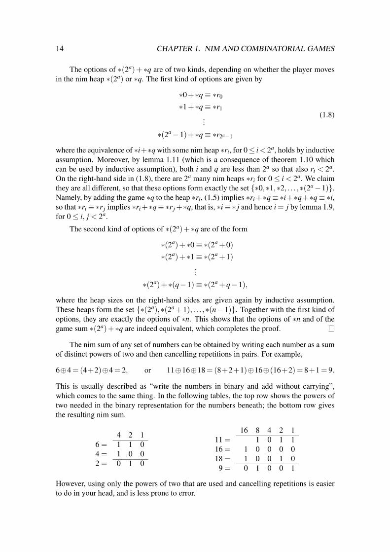
The nim sum of any set of numbers can be obtained by writing each number as a sumof distinct powers of two and then cancelling repetitions in pairs. For example,
6⊕4 = (4+2)⊕4 = 2, or 11⊕16⊕18 = (8+2+1)⊕16⊕(16+2) = 8+1 = 9.
This is usually described as “write the numbers in binary and add without carrying”,which comes to the same thing. In the following tables, the top row shows the powers oftwo needed in the binary representation for the numbers beneath; the bottom row givesthe resulting nim sum.
4 2 16 = 1 1 04 = 1 0 02 = 0 1 0
16 8 4 2 111 = 1 0 1 116 = 1 0 0 0 018 = 1 0 0 1 09 = 0 1 0 0 1
However, using only the powers of two that are used and cancelling repetitions is easierto do in your head, and is less prone to error.

1.10. SUMS OF NIM HEAPS 15
How does theorem 1.10 translate into playing nim? When the nim sum of the heapsizes is zero, then the player is in a losing position. (Such nim positions are sometimescalled balanced positions.) All moves will lead to a winning position, and in practice thebest advice may only be not to move to a winning position that is too obvious, like onewhere two heap sizes are equal, in the hope that the opponent makes a mistake.
If the nim sum of the heap sizes is not zero, it is some sum of powers of two, says = 2a + 2b + 2c + · · ·, like for example 11⊕ 16⊕ 18 = 9 = 8 + 1 above. The winningmove is then obtained as follows:
1. Identify a heap of size n which uses 2a, the largest power of 2 in the nim sum; at leastone such heap must exist. In the example, that heap has size 11 (so it is not alwaysthe largest heap).
2. Compute n⊕ s. In that nim sum, the power 2a appears in both n and s, and it cancelsout, so the result is some number m that is smaller than n. In the example, m =11⊕9 = (8+2+1)⊕ (8+1) = 2.
3. Reduce the heap of size n to size m, in the example from size 11 to size 2. Theresulting heap ∗m is equivalent to ∗n+∗s, so when it replaces ∗n in the original sum,∗s is added and cancels with ∗s, and the result is equivalent to ∗0, a losing position.
On paper, the binary representation may be easier to use. In step 2 above, computingn⊕s amounts to “flipping the bits” in the binary representation of the heap n whenever thecorresponding bit in the binary representation of the sum s is one. In this way, a playerin a winning position moves always from an “unbalanced” position (with nonzero nimsum) to a balanced position (nim sum zero), which is losing because any move will createagain an unbalanced position. This is the way nim is usually explained. The method wasdiscovered by Bouton who published it in 1902.
⇒ You are now in a position to answer all of exercise 1.1 on page 20.
So far, it is not fully clear why powers of two appear in the computation of nimsums. One reason is provided by the proof of theorem 1.10. The options of moving from∗(2a)+ ∗q in (1.8) neatly produce exactly the numbers 0,1, . . . ,2a− 1, which would notwork when replacing 2a with something else.
As a second reason, the copycat principle G+G≡ ∗0 shows that the impartial gamesform a group where every element is its own inverse. There is essentially only one math-ematical structure that has these particular properties, namely the addition of binary vec-tors. In each component, such vectors are separately added modulo two, where 1⊕1 = 0.Here, the binary vectors translate into binary numbers for the sizes of the nim heaps. The“addition without carry” of binary vectors defines exactly the winning strategy in nim, asstated in theorem 1.10. However, the proof of this theorem is stated directly and withoutany recourse to abstract algebra and groups.
A third reason uses the construction of equivalent nim heaps for any impartial game,in particular a sum of two nim heaps, which we explain next; see also figure 1.2 below.

16 CHAPTER 1. NIM AND COMBINATORIAL GAMES
1.11 Poker nim and the mex rule
Poker nim is played with heaps of poker chips. Just as in ordinary nim, either player mayreduce the size of any heap by removing some of the chips. But alternatively, a playermay also increase the size of some heap by adding to it some of the chips he acquired inearlier moves. These two kinds of moves are the only ones allowed.
Let’s suppose that there are three heaps, of sizes 3,4,5, and that the game has beengoing on for some time, so that both players have accumulated substantial reserves ofchips. It’s player I’s turn, who moves to 1,4,5 because that is a good move in ordinarynim. But now player II adds 50 chips to the heap of size 4, creating position 1,54,5,which seems complicated.
What should player I do? After a moment’s thought, he just removes the 50 chipsplayer II has just added to the heap, reverting to the previous position. Player II may keepadding chips, but will eventually run out of them, no matter how many she acquires inbetween, and then player I can proceed as in ordinary nim.
So a player who can win a position in ordinary nim can still win in poker nim. Hereplies to the opponent’s reducing moves just as he would in ordinary nim, and reversesthe effect of any increasing move by using a reducing move to restore the heap to thesame size again. Strictly speaking, the ending condition (see condition 6 in section 1.6) isviolated in poker nim because in theory the game could go on forever. However, a playerin a winning position wants to end the game with his victory, and never has to put backany chips; then the losing player will eventually run out of chips that she can add to aheap, so that the game terminates.
Consider now an impartial game where the options of player I are games that areequivalent to the nim heaps ∗0, ∗1, ∗2, ∗5, ∗9. This can be regarded as a rather peculiarnim heap of size 3 which can be reduced to any of the sizes 0,1,2, but which can also beincreased to size 5 or 9. The poker nim argument shows that this extra freedom is in factof no use whatsoever.
The mex rule says that if the options of a game G are equivalent to nim heaps withsizes from a set S (like S = {0,1,2,5,9} above), then G is equivalent to a nim heap ofsize m, where m is the smallest non-negative integer not contained in S. This number mis written mex(S), where mex stands for “minimum excludant”. That is,
m = mex(S) = min{k ≥ 0 | k 6∈ S}. (1.9)
For example, mex({0,1,2,3,5,6}) = 4, mex({1,2,3,4,5}) = 0, and mex( /0) = 0.
⇒ Which game has the empty set /0 as its set of options?
Theorem 1.12 (The mex rule) Let the impartial game G have the set of options that areequivalent to {∗s | s ∈ S} for some set S of non-negative integers (assuming S is not theset of all non-negative integers, for example if S is finite). Then G≡ ∗(mex(S)).
Proof. Let m = mex(S). We show G+∗m≡ ∗0, which proves the theorem by lemma 1.7.If player I moves from G+∗m to G+∗k for some k < m, then k ∈ S and there is an option

1.12. FINDING NIM VALUES 17
K of G so that K ≡ ∗k by assumption, so player II can counter by moving from G + ∗kto the losing position K +∗k. Otherwise, player I may move to K +∗m, where K is someoption K which is equivalent to ∗k for some k ∈ S. If k < m, then player II counters bymoving to K +∗k. If k > m, then player II counters by moving to M +∗m where M is theoption of K that is equivalent to ∗m (because K ≡ ∗k). The case k = m is excluded by thedefinition of m = mex(S). This shows G+∗m is a losing game.
A special case of the preceding theorem is that mex(S) = 0, which means that alloptions of G are equivalent to positive nim heaps, so they are all winning positions, orthat G has no options at all. Then G is a losing game, and indeed G≡ ∗0.
Corollary 1.13 Any impartial game G is equivalent to some nim heap ∗n.
Proof. We can assume by induction that this holds for all games that are simpler than G,in particular the options of G. They are equivalent to nim heaps whose sizes form the set S(which we assume is not the set of all non-negative integers). Theorem 1.12 then showsG≡ ∗m for m = mex(S).
⇒ Do exercise 1.7 on page 23, which provides an excellent way to understand the mexrule.
1.12 Finding nim values
By corollary 1.13, any impartial game can be played like nim, provided the equivalent nimheaps of the positions of the game are known. This forms the basis of the Sprague–Grundytheory of impartial games, named after the independent discoveries of this principle byR. P. Sprague in 1936 and P. M. Grundy in 1939. Any sum of such games is then evaluatedby taking the nim sum of the sizes of the corresponding nim heaps.
The nim values of the positions can be evaluated by the mex rule (theorem 1.12).This is illustrated in the “rook-move” game in figure 1.1. Place a rook on a chess boardof given arbitrary size. In one move, the rook is moved either horizontally to the leftor vertically upwards, for any number of squares (at least one) as long as it stays on theboard. The first player who can no longer move loses, when the rook is on the top leftsquare of the board. We number the rows and columns of the board by 0,1,2, . . . startingfrom the top left.
Figure 1.2 gives the nim values for the positions of the rook on the chess board. Thetop left square is equivalent to ∗0 because the rook can no longer move. The squarebelow that allows only to reach the square with ∗0 on it, so it is equivalent to ∗1 becausemex{0} = 1. The square below gets ∗2 because its options are equivalent to ∗0 and ∗1.From any square in the leftmost column in figure 1.2, the rook can only move upwards, soany such square in row i corresponds obviously to a nim heap ∗i. Similarly, the topmostrow has entry ∗ j in column j.
In general, a position on the board is evaluated knowing all nim values for the squaresto the left and the top of it, which are the options of that position. As an example, consider

18 CHAPTER 1. NIM AND COMBINATORIAL GAMES
0
1
2
3
4
5
0 1 2 3 4 5 6 7
Figure 1.1 Rook move game, where the player may move the rook on the chess boardin the direction of the arrows.
the square in row 3 and column 2. To the left of that square, the entries ∗3 and ∗2 arefound, and to the top the entries ∗2,∗3,∗0. So the square itself is equivalent to ∗1 becausemex({0,2,3}) = 1. The square in row 3 and column 5, where the rook is placed infigure 1.1, gets entry ∗6.
0
1
2
3
4
5
6
7
8
9
10
0 1 2 3 4 5 6 7 8 9 10
∗0
∗1
∗2
∗3
∗4
∗5
∗6
∗7
∗8
∗9
∗10
∗1
∗0
∗3
∗2
∗5
∗4
∗7
∗6
∗9
∗8
∗11
∗2
∗3
∗0
∗1
∗6
∗7
∗4
∗5
∗10
∗11
∗8
∗3
∗2
∗1
∗0
∗7
∗6
∗5
∗4
∗11
∗10
∗9
∗4
∗5
∗6
∗7
∗0
∗1
∗2
∗3
∗12
∗13
∗14
∗5
∗4
∗7
∗6
∗1
∗0
∗3
∗2
∗13
∗12
∗15
∗6
∗7
∗4
∗5
∗2
∗3
∗0
∗1
∗14
∗15
∗12
∗7
∗6
∗5
∗4
∗3
∗2
∗1
∗0
∗15
∗14
∗13
∗8
∗9
∗10
∗11
∗12
∗13
∗14
∗15
∗0
∗1
∗2
∗9
∗8
∗11
∗10
∗13
∗12
∗15
∗14
∗1
∗0
∗3
∗10
∗11
∗8
∗9
∗14
∗15
∗12
∗13
∗2
∗3
∗0
Figure 1.2 Equivalent nim heaps ∗n for positions of the rook move game.
The astute reader will have noticed that the rook move game is just nim with twoheaps. A rook positioned in row i and column j can either diminish i by moving left, or j
1.12. FINDING NIM VALUES 19
by moving up. So this position is the sum of nim heaps ∗i+∗ j. It is a losing position if andonly if i = j, where the rook is on the diagonal leading to the top left square. Therefore,figure 1.2 represents the computation of nim heaps equivalent to ∗i +∗ j, or, by omittingthe stars, the nim sums i⊕ j, for all i, j ≥ 0.
The nim addition table figure 1.2 is computed by the mex rule, and does not requiretheorem 1.10. Given this nim addition table, one can conjecture (1.7). You may find ituseful to go back to the proof of theorem 1.10 using figure 1.2 and check the options fora position of the form ∗(2a)+∗q for q < 2a, as a square in row 2a and column q.
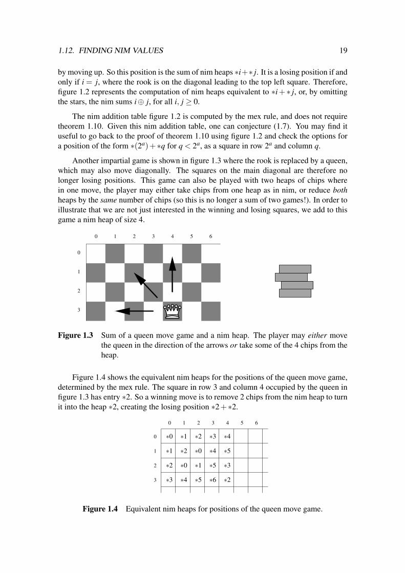
Another impartial game is shown in figure 1.3 where the rook is replaced by a queen,which may also move diagonally. The squares on the main diagonal are therefore nolonger losing positions. This game can also be played with two heaps of chips wherein one move, the player may either take chips from one heap as in nim, or reduce bothheaps by the same number of chips (so this is no longer a sum of two games!). In order toillustrate that we are not just interested in the winning and losing squares, we add to thisgame a nim heap of size 4.
0
1
2
3
0 1 2 3 4 5 6
Figure 1.3 Sum of a queen move game and a nim heap. The player may either movethe queen in the direction of the arrows or take some of the 4 chips from theheap.
Figure 1.4 shows the equivalent nim heaps for the positions of the queen move game,determined by the mex rule. The square in row 3 and column 4 occupied by the queen infigure 1.3 has entry ∗2. So a winning move is to remove 2 chips from the nim heap to turnit into the heap ∗2, creating the losing position ∗2+∗2.
0
1
2
3
0 1 2 3 4 5 6
∗0
∗1
∗2
∗3
∗1
∗2
∗0
∗4
∗2
∗0
∗1
∗5
∗3
∗4
∗5
∗6
∗4
∗5
∗3
∗2
Figure 1.4 Equivalent nim heaps for positions of the queen move game.

20 CHAPTER 1. NIM AND COMBINATORIAL GAMES
This concludes our introduction to combinatorial games. Further examples will begiven in the exercises.
⇒ Do the remaining exercises 1.4–1.11, starting on page 21, which show how to usethe mex rule and what you learned about nim and combinatorial games.
1.13 Exercises for chapter 1
In this chapter, which is more abstract than the others, the exercises are particularly im-portant. Exercise 1.1 is a standard question on nim, where part (a) can be answered evenwithout the theory. Exercise 1.2 is an example of an impartial game, which can also be an-swered without much theory. Exercise 1.3 is difficult – beware not to rush into any quickand false application of nim values here; part (c) of this exercise is particularly challeng-ing. Exercise 1.4 tests your understanding of the queen move game. For exercise 1.5,remember the concept of a sum of games, which applies here naturally. In exercise 1.6,try to see how nim heaps are hidden in the game. Exercise 1.7 is very instructive for un-derstanding the mex rule. In exercise 1.8, it is essential that you understand nim values. Ittakes some work to investigate all the options in the game. Exercise 1.9 is another famil-iar game where you have to find out nim values. In exercise 1.10, a new game is definedthat you can analyse with the mex rule. Exercise 1.11 is an impartial game that is ratherdifferent from the previous games. In the challenging part (c) of that exercise, you shouldfirst formulate a conjecture and then prove it precisely.
Exercise 1.1 Consider the game nim with heaps of chips. The players alternately removesome chips from one of the heaps. The player to remove the last chip wins.(a) For all positions with three heaps, where one of the heaps has only one chip, describe
exactly the losing positions. Justify your answer, for example with a proof by induc-tion, or by theorems on nim.[Hint: Start with the easy cases to find the pattern.]
(b) Determine all initial winning moves for nim with three heaps of size 6, 10 and 15,using the theorem on nim where the heap sizes are represented as sums of powers oftwo.
Exercise 1.2 The game dominos is played on a board of m× n squares, where playersalternately place a domino on the board which covers two adjacent squares that are free(not yet occupied by a domino), vertically or horizontally. The first player who cannotplace a domino any more loses. Example play for a 2×3 board:
Iloses
II I
(a) Who will win in 3×3 dominos?[Hint: Use the symmetry of the game to investigate possible moves, and rememberthat it suffices to find one winning strategy.]

1.13. EXERCISES FOR CHAPTER 1 21
(b) Who will win in m×n dominos when both m and n are even?
(c) Who will win in m×n dominos when m is odd and n is even?
Justify your answers.
Note (not a question): Because of the known answers from (b) and (c), this gameis more interesting for “real play” on an m× n board where both m and n are odd. Playit with your friends on a 5× 5 board, for example. The situation often decomposes intoindependent parts, like contiguous fields of 2, 3, 4, 5, 6 squares, that have a known winner,which may help you analyse the situation.
Exercise 1.3 Consider the following game chomp: A rectangular array of m× n dots isgiven, in m rows and n columns, like 3×4 in the next picture on the left. A dot in row iand column j is named (i, j). A move consists in picking a dot (i, j) and removing it andall other dots to the right and below it, which means removing all dots (i′, j′) with i′ ≥ iand j′ ≥ j, as shown for (i, j) = (2,3) in the middle picture, resulting in the picture on theright:
Player I is the first player to move, players alternate, and the last player who removesa dot loses.
An alternative way is to think of these dots as (real) cookies: a move is to eat acookie and all those to the right and below it, but the top left cookie is poisoned. See alsohttp://www.stolaf.edu/people/molnar/games/chomp/
(a) Assuming optimal play, determine the winning player and a winning move for chompof size 2×2, size 2×3, size 2×n, and size m×m, where m≥ 3. Justify your answers.
(b) In the way described here, chomp is a misere game where the last player to makea move loses. Suppose we want to play the same game so that the normal playconvention applies, where the last player to move wins. (This would be a boringgame with the board as given, by simply taking the top left dot (1,1).) Explain howthis can be done by removing one dot from the initial array of dots.
(c) Show that when chomp is played for a game of any size m× n, player I can alwayswin.[Hint: You only have to show that a winning move exists, but you do not have todescribe that winning move.]
Exercise 1.4(a) Complete the entries of equivalent nim heaps for the queen move game in columns 5
and 6, rows 0 to 3, in the table in figure 1.4.
(b) Describe all winning moves in the game-sum of the queen move game and the nimheap in figure 1.3.

22 CHAPTER 1. NIM AND COMBINATORIAL GAMES
Exercise 1.5 Consider the game dominos from exercise 1.2, played on a 1×n board forn≥ 2. Let Dn be the nim value of that game, so that the starting position of the 1×n boardis equivalent to a nim heap of size Dn. For example, D2 = 1 because the 1× 2 board isequivalent to ∗1.
(a) How is Dn computed from smaller values Dk for k < n?[Hint: Use sums of games and the mex rule. The notation for nim sums is ⊕, wherea⊕b = c if and only if ∗a+∗b≡ ∗c.]
(b) Give the values of Dn up to n = 10 (or more, if you are ambitious – higher valuescome at n = 16, and at some point they even repeat, but before you detect that youwill probably have run out of patience). For which values of n, where 1≤ n≤ 10, isdominos on a 1×n board a losing game?
Exercise 1.6 Consider the following game on a rectangular board where a white and ablack counter are placed in each row, like in this example:
8
5
4
a b d e gc f h
1
2
3
6
7
(*)
Player I is white and starts, and player II is black. Players take turns. In a move, aplayer moves a counter of his colour to any other square within its row, but may not jumpover the other counter. For example, in (*) above, in row 8 white may move from e8 toany of the squares c8, d8, f8, g8, or h8. The player who can no longer move loses.
(a) Who will win in the following position?
8
5
4
a b d e gc f h
1
2
3
6
7
(b) Show that white can win in position (*) above. Give at least two winning moves fromthat position.
Justify your answers.[Hint: Compare this with another game that is not impartial and that also violates the

1.13. EXERCISES FOR CHAPTER 1 23
ending condition, but that nevertheless is close to nim and ends in finite time whenplayed well.]
Exercise 1.7 Consider the following network (in technical terms, a directed graph or “di-graph”). Each circle, here marked with one of the letters A–P, represents a node of thenetwork. Some of these nodes (here A, F, G, H, and K) have counters on them, whichare allowed to share a node, like the two counters on H. In a move, one of the countersis moved to a neighbouring node in the direction of the arrow as indicated, for examplefrom F to I (but not from F to C, nor directly from F to D, say). Players alternate, and thelast player no longer able to move loses.
I
M
P
L
H
E
F
G
J
K
N
O
A
B
C
D
(a) Explain why this game fulfils the ending condition.
(b) Who is winning in the above position? If it is player I (the first player to move),describe all possible winning moves. Justify your answer.
(c) How does the answer to (b) change when the arrow from J to K is reversed so that itpoints from K to J instead?
Exercise 1.8 Consider the game chomp from Exercise 1.3 of size 2× 4, added to a nimheap of size 4.
What are the winning moves of the starting player I, if any?[Hint: Represent chomp as a game in the normal play convention (see exercise 1.3(b),by changing the dot pattern), so that the losing player is not the player who takes the“poisoned cookie”, but the player who can no longer move. This will simplify finding thevarious nim values.]
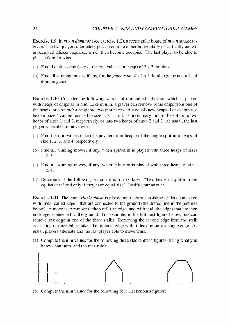
24 CHAPTER 1. NIM AND COMBINATORIAL GAMES
Exercise 1.9 In m×n dominos (see exercise 1.2), a rectangular board of m×n squares isgiven. The two players alternately place a domino either horizontally or vertically on twounoccupied adjacent squares, which then become occupied. The last player to be able toplace a domino wins.
(a) Find the nim-value (size of the equivalent nim heap) of 2×3 dominos.
(b) Find all winning moves, if any, for the game-sum of a 2×3 domino game and a 1×4domino game.
Exercise 1.10 Consider the following variant of nim called split-nim, which is playedwith heaps of chips as in nim. Like in nim, a player can remove some chips from one ofthe heaps, or else split a heap into two (not necessarily equal) new heaps. For example, aheap of size 4 can be reduced to size 3, 2, 1, or 0 as in ordinary nim, or be split into twoheaps of sizes 1 and 3, respectively, or into two heaps of sizes 2 and 2. As usual, the lastplayer to be able to move wins.
(a) Find the nim-values (size of equivalent nim heaps) of the single split-nim heaps ofsize 1, 2, 3, and 4, respectively.
(b) Find all winning moves, if any, when split-nim is played with three heaps of sizes1, 2, 3.
(c) Find all winning moves, if any, when split-nim is played with three heaps of sizes1, 2, 4.
(d) Determine if the following statement is true or false: “Two heaps in split-nim areequivalent if and only if they have equal size.” Justify your answer.
Exercise 1.11 The game Hackenbush is played on a figure consisting of dots connectedwith lines (called edges) that are connected to the ground (the dotted line in the picturesbelow). A move is to remove (“chop off”) an edge, and with it all the edges that are thenno longer connected to the ground. For example, in the leftmost figure below, one canremove any edge in one of the three stalks. Removing the second edge from the stalkconsisting of three edges takes the topmost edge with it, leaving only a single edge. Asusual, players alternate and the last player able to move wins.
(a) Compute the nim values for the following three Hackenbush figures (using what youknow about nim, and the mex rule):
, , .
(b) Compute the nim values for the following four Hackenbush figures:

1.13. EXERCISES FOR CHAPTER 1 25
, , , .
(c) Based on the observation in (b), give a rule how to compute the nim value of a “tree”which is constructed by putting several “branches” with known nim values on topof a “stem” of size n, for example n = 2 in the picture below, where three branchesof height 3, 2, and 4 are put on top of the “stem”. Prove that rule (you may find itadvantageous to glue the branches together at the bottom, as in (b)). Use this to findthe nim value of the rightmost picture.
of becomeson top
.

26 CHAPTER 1. NIM AND COMBINATORIAL GAMES

Chapter 2
Games as trees and in strategic form
This chapter introduces the main concepts of non-cooperative game theory: game treesand games in strategic form and the ways to analyse them.
We occasionally refer to concepts discussed in chapter 1, such as “game states”, toclarify the connection, but chapter 1 is not a requirement to study this chapter.
2.1 Learning objectives
After studying this chapter, you should be able to:
• interpret game trees and games in strategic form;
• explain the concepts of move in a game tree, strategy (and how it differs from move),strategy profile, backward induction, symmetric games, dominance and weak domi-nance, dominance solvable, Nash equilibrium, reduced strategies and reduced strate-gic form, subgame perfect Nash equilibrium, and commitment games;
• apply these concepts to specific games.
2.2 Further reading
The presented concepts are standard in game theory. They can be found, for example, inthe following book:
• Osborne, Martin J., and Ariel Rubinstein A Course in Game Theory. (MIT Press,1994) [ISBN 0262650401].
Osborne and Rubinstein treat game theory as it is used in economics. Rubinstein isalso a pioneer of bargaining theory. He invented the alternating-offers model treated inchapter 5. On the other hand, the book uses some non-standard descriptions. For example,Osborne and Rubinstein define games of perfect information via “histories” and not gametrees; we prefer the latter because they are less abstract. Hence, keep in mind that the
27

28 CHAPTER 2. GAMES AS TREES AND IN STRATEGIC FORM
terminology used by Osborne and Rubinstein may not be standard and may differ fromours.
Another possible reference is:
• Gibbons, Robert A Primer in Game Theory [in the United States sold under the titleGame Theory for Applied Economists]. (Prentice Hall / Harvester Wheatsheaf, 1992)[ISBN 0745011594].
In particular, this book looks at the commitment games of section 2.14 from theeconomic perspective of “Stackelberg leadership”.
2.3 Introduction
In this chapter, we introduce several main concepts of non-cooperative game theory: gametrees (with perfect information), which describe explicitly how a game evolves over time,and strategies, which describe a player’s possible “plans of action”. A game can be de-scribed in terms of strategies alone, which defines a game in strategic form.
Game trees can be solved by backward induction, where one finds optimal movesfor each player, given that all future moves have already been determined. The centralconcept for games in strategic form is the Nash equilibrium, where each player choosesa strategy that is optimal given what the other players are doing. We will show thatbackward induction always produces a Nash equilibrium, also called “subgame perfectNash equilibrium” or SPNE.
The main difference between game trees and games in strategic form is that in a gametree, players act sequentially, being aware of the previous moves of the other players. Incontrast, players in a game in strategic form move simultaneously. The difference betweenthese two descriptions becomes striking when changing a two-player game in strategicform to a game with commitment, described by a game tree where one player moves firstand the other second, but which otherwise has the same payoffs.
Every game tree can be converted to strategic form, which, however, is often muchlarger than the tree. A general game in strategic form can only be represented by a tree bymodelling “imperfect information” where a player is not aware of another player’s action.Game trees with imperfect information are treated in chapter 4.
2.4 Definition of game trees
Figure 2.1 shows an example of a game tree. We always draw trees downwards, with theroot at the top. (Conventions on drawing game trees vary. Sometimes trees are drawnfrom the bottom upwards, sometimes from left to right, and sometimes from the centerwith edges in any direction.)
The nodes of the tree denote game states. (In a combinatorial game, game states arecalled “positions”.) Nodes are connected by lines, called edges. An edge from a node u
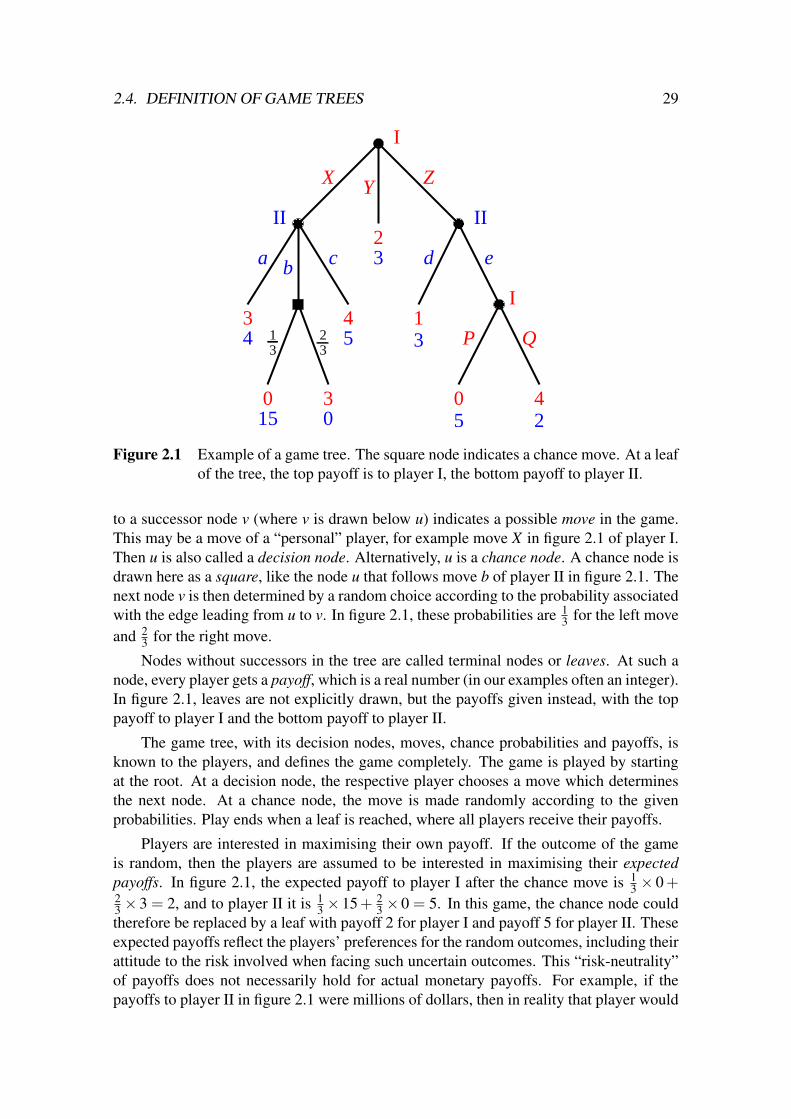
2.4. DEFINITION OF GAME TREES 29
����
����
����
����
3 321
3 4 1
0 3 0 4
QP
I
ZYX
23 d ecba
15
4 5
0
3
5 2
II II
I
Figure 2.1 Example of a game tree. The square node indicates a chance move. At a leafof the tree, the top payoff is to player I, the bottom payoff to player II.
to a successor node v (where v is drawn below u) indicates a possible move in the game.This may be a move of a “personal” player, for example move X in figure 2.1 of player I.Then u is also called a decision node. Alternatively, u is a chance node. A chance node isdrawn here as a square, like the node u that follows move b of player II in figure 2.1. Thenext node v is then determined by a random choice according to the probability associatedwith the edge leading from u to v. In figure 2.1, these probabilities are 1
3 for the left moveand 2
3 for the right move.
Nodes without successors in the tree are called terminal nodes or leaves. At such anode, every player gets a payoff, which is a real number (in our examples often an integer).In figure 2.1, leaves are not explicitly drawn, but the payoffs given instead, with the toppayoff to player I and the bottom payoff to player II.
The game tree, with its decision nodes, moves, chance probabilities and payoffs, isknown to the players, and defines the game completely. The game is played by startingat the root. At a decision node, the respective player chooses a move which determinesthe next node. At a chance node, the move is made randomly according to the givenprobabilities. Play ends when a leaf is reached, where all players receive their payoffs.
Players are interested in maximising their own payoff. If the outcome of the gameis random, then the players are assumed to be interested in maximising their expectedpayoffs. In figure 2.1, the expected payoff to player I after the chance move is 1
3 × 0 +23 ×3 = 2, and to player II it is 1
3 ×15 + 23 ×0 = 5. In this game, the chance node could
therefore be replaced by a leaf with payoff 2 for player I and payoff 5 for player II. Theseexpected payoffs reflect the players’ preferences for the random outcomes, including theirattitude to the risk involved when facing such uncertain outcomes. This “risk-neutrality”of payoffs does not necessarily hold for actual monetary payoffs. For example, if thepayoffs to player II in figure 2.1 were millions of dollars, then in reality that player would

30 CHAPTER 2. GAMES AS TREES AND IN STRATEGIC FORM
probably prefer receiving 5 million dollars for certain to a lottery that gave her 15 milliondollars with probability 1/3 and otherwise nothing. However, payoffs can be adjusted toreflect the player’s attitude to risk, as well as representing the “utility” of an outcome likemoney so that one can take just the expectation. In the example, player II may consider alottery that gives her 15 million dollars with probability 1/3 and otherwise nothing onlyas a valuable as getting 2 million dollars for certain. In that case, “15 million dollars” maybe represented by a payoff of 6 so that the said lottery has an expected payoff 2, assumingthat “2 million dollars” are represented by a payoff of 2 and “getting nothing” by a payoffof 0. This is discussed in greater detail in section 3.4.
(a) (b)����
����
����
����
����
����
2
a
0
II
P A
II
02
11
11
A P
1 2
a
1 0
II
AP AP
II
02
p p
Figure 2.2 The left picture (a) is not a tree because the leaf where both players receivepayoff 1 is reachable by two different paths. The correct tree representationis shown on the right in (b).
For the game tree, it does not matter how it is drawn, but only its “combinatorial”structure, that is, how its nodes are connected by edges. A tree can be considered asa special “directed graph”, given by a set of nodes, and a set of edges, which are pairsof nodes (u,v). A path in such a graph from node u to node v is a sequence of nodesu0u1 . . .uk so that u0 = u, uk = v, and so that (ui,ui+1) is an edge for 0≤ i < k. The graphis a tree if it has a distinguished node, the root, so that to each node of the graph there isa unique path from the root.
Figure 2.2 demonstrates the tree property that every node is reached by a unique pathfrom the root. This fails to hold in the left picture (a) for the middle leaf. Such a structuremay make sense in a game. For example, the figure could represent two people in apub where first player II chooses to pay for the drinks (move p) or to accept (move a)that the first round is paid by player I. In the second round, player I may then decideto either accept not to pay (move A) or to pay (P). Then the players may only care howoften, but not when, they have paid a round, with the middle payoff pair (1,1) for twopossible “histories” of moves. The tree property prohibits game states with more thanone history, because the history is represented by the unique path from the root. Even ifcertain differences in the game history do not matter, these game states are distinguished,mostly as a matter of mathematical convenience. The correct representation of the abovegame is shown in the right picture, figure 2.2(b).
Game trees are also called extensive games with perfect information. Perfect informa-tion means that a player always knows the game state and therefore the complete history

2.5. BACKWARD INDUCTION 31
of the game up to then. Game trees can be enhanced with an additional structure thatrepresents “imperfect information”, which is the topic of chapter 4.
Note how game trees differ from the combinatorial games studied in chapter 1:
(a) A combinatorial game can be described very compactly, in particular when it is givenas a sum of games. For general game trees, such sums are typically not considered.
(b) The “rules” in a game tree are much more flexible: more than two players and chancemoves are allowed, players do not have to alternate, and payoffs do not just stand for“win” or “lose”.
(c) The flexibility of game trees comes at a price, though: The game description is muchlonger than a combinatorial game. For example, a simple instance of nim may requirea huge game tree. Regularities like the mex rule do not apply to general game trees.
2.5 Backward induction
Which moves should the players choose in a game tree? “Optimal” play should maximisea player’s payoff. This can be decided irrespective of other players’ actions when theplayer is the last player to move. In figure 2.2(b), player I maximises his payoff bymove A at both his decision nodes, because at the left node he receives 1 rather than 0with that move, and at the right node payoff 2 rather than 1. Going backwards in time,player II has to make her move a or p at the root of the game tree, where she will receiveeither 1 or 0, assuming the described future behaviour of player I. Consequently, she willchoose a.
This process is called backward induction: Starting with the decision nodes closestto the leaves, a player’s move is chosen which maximises that player’s payoff at the node.In general, a move is chosen in this way for each decision node provided all subsequentmoves have already been decided. Eventually, this will determine a move for every deci-sion node, and hence for the entire game. Backward induction is also known as Zermelo’salgorithm. (This is attributed to an article by Zermelo (1913) on chess. Later, peopledecided that Zermelo proved something different, in fact a more complicated property, sothat Zermelo’s algorithm is sometimes called “Kuhn’s algorithm”, according to a paperby Kuhn (1953), which we cite on page 96.)
The move selected by backward induction is not necessarily unique, if there is morethan one move giving maximal payoff to the player. In the game in figure 2.1, backwardinduction chooses either move b or move c for player II, both of which give her payoff 5(which is an expected payoff for move b) that exceeds her payoff 4 for move a. At theright-most node, player I chooses Q. This determines the preceding move d by player IIwhich gives her the higher payoff 3 as opposed to 2 (via move Q). In turn, this meansthat player I, when choosing between X , Y , or Z at the root of the game tree, will getpayoff 2 for Y and payoff 1 for Z; the payoff when he chooses X depends on the choiceof player II: if that is b, then player I gets 2, and can choose either X or Y , both of whichgive him maximal payoff 2. If player II chooses c, however, then the payoff to player Iis 4 when choosing X , so this is the unique optimal choice. To summarise, the possible

32 CHAPTER 2. GAMES AS TREES AND IN STRATEGIC FORM
combinations of moves that can arise in figure 2.1 by backward induction are, simplylisting the moves for each player: (XQ,bd), (XQ,cd), and (Y Q,bd). Note that Q andd are always chosen, but that Y can only be chosen in combination with the move b byplayer II.
The moves determined by backward induction are therefore, in general, not unique,and possibly interdependent.
Backward induction gives a unique recommendation to each player if there is alwaysonly one move that gives maximal payoff. This applies to generic games. A generic gameis a game where the payoff parameters are real numbers that are in no special dependencyof each other (like two payoffs being equal). In particular, it should be allowed to replacethem with values nearby. For example, the payoffs may be given in some practical sce-nario which has some “noise” that effects the precise value of each payoff. Then two suchpayoffs are equal with probability zero, and so this case can be disregarded. In genericgames, the optimal move is always unique, so that backward induction gives a uniqueresult.
2.6 Strategies and strategy profiles
Definition 2.1 In a game tree, a strategy of a player specifies a move for every decisionnode of that player. A strategy profile is a tuple of strategies, with one strategy for eachplayer of the game.
If the game has only two players, a strategy profile is therefore a pair of strategies,with one strategy for player I and one strategy for player II.
In the game tree in figure 2.1, the possible strategies for player I are XP, XQ, Y P, Y Q,ZP, ZQ. The strategies for player II are ad, ae, bd, be, cd, ce. For simplicity of notation,we have thereby specified a strategy simply as a list of moves, one for each decision nodeof the player. When specifying a strategy in that way, this must be done with respect to afixed order of the decision nodes in the tree, in order to identify each move uniquely. Thismatters when a move name appears more than once, for example in figure 2.2(b). In thattree, the strategies of player I are AA, AP, PA, PP, with the understanding that the firstmove refers to the left decision node and the second move to the right decision node ofplayer I.
Backward induction defines a move for every decision node of the game tree, andtherefore for every decision node of each player, which in turn gives a strategy for eachplayer. The result of backward induction is therefore a strategy profile.
⇒ Exercise 2.1 on page 52 studies a game tree which is not unlike the game in fig-ure 2.1. You can already answer part (a) of this exercise, and apply backward in-duction, which answers (e).
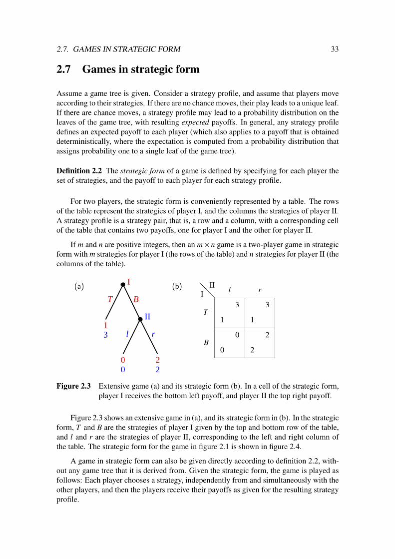
2.7. GAMES IN STRATEGIC FORM 33
2.7 Games in strategic form
Assume a game tree is given. Consider a strategy profile, and assume that players moveaccording to their strategies. If there are no chance moves, their play leads to a unique leaf.If there are chance moves, a strategy profile may lead to a probability distribution on theleaves of the game tree, with resulting expected payoffs. In general, any strategy profiledefines an expected payoff to each player (which also applies to a payoff that is obtaineddeterministically, where the expectation is computed from a probability distribution thatassigns probability one to a single leaf of the game tree).
Definition 2.2 The strategic form of a game is defined by specifying for each player theset of strategies, and the payoff to each player for each strategy profile.
For two players, the strategic form is conveniently represented by a table. The rowsof the table represent the strategies of player I, and the columns the strategies of player II.A strategy profile is a strategy pair, that is, a row and a column, with a corresponding cellof the table that contains two payoffs, one for player I and the other for player II.
If m and n are positive integers, then an m×n game is a two-player game in strategicform with m strategies for player I (the rows of the table) and n strategies for player II (thecolumns of the table).
����
����
1
0 2
3
0 2
I
II
rl
T B @@@I
II
T
B
l r
1 1
3 3
0 2
0 2
(b)(a)
Figure 2.3 Extensive game (a) and its strategic form (b). In a cell of the strategic form,player I receives the bottom left payoff, and player II the top right payoff.
Figure 2.3 shows an extensive game in (a), and its strategic form in (b). In the strategicform, T and B are the strategies of player I given by the top and bottom row of the table,and l and r are the strategies of player II, corresponding to the left and right column ofthe table. The strategic form for the game in figure 2.1 is shown in figure 2.4.
A game in strategic form can also be given directly according to definition 2.2, with-out any game tree that it is derived from. Given the strategic form, the game is played asfollows: Each player chooses a strategy, independently from and simultaneously with theother players, and then the players receive their payoffs as given for the resulting strategyprofile.

34 CHAPTER 2. GAMES AS TREES AND IN STRATEGIC FORM
@@@I
II
XP
XQ
Y P
Y Q
ZP
ZQ
ad ae bd be cd ce
3 3 2 2 4 4
4 4 5 5 5 5
3 3 2 2 4 4
4 4 5 5 5 5
2 2 2 2 2 2
3 3 3 3 3 3
2 2 2 2 2 2
3 3 3 3 3 3
1 0 1 0 1 0
3 5 3 5 3 5
1 4 1 4 1 4
3 2 3 2 3 2
Figure 2.4 Strategic form of the extensive game in figure 2.1. The less redundant re-duced strategic form is shown in figure 2.13 below.
2.8 Symmetric games
Many game-theoretic concepts are based on the strategic form alone. In this section, wediscuss the possible symmetries of such a game. We do this by presenting a number ofstandard games from the literature, mostly 2× 2 games, which are the smallest gameswhich are not just one-player decision problems.
@@@I
II
C
D
c d
2 0
2 3
3 1
0 1
(a)@
@@I
II
C
D
c d
2 0
2 3
3 1
0 1
..................................................
(b)
Figure 2.5 Prisoner’s dilemma game (a), its symmetry shown by reflection along thedotted diagonal line in (b).
Figure 2.5(a) shows the well-known “prisoner’s dilemma” game. Each player hastwo strategies, called C and D for player I and c and d for player II. (We use upper

2.8. SYMMETRIC GAMES 35
case letters for player I and lower case letters for player II for easier identification ofstrategies and moves.) These letters stand for “cooperate” and “defect”, respectively. Thestory behind the name “prisoner’s dilemma” is that of two prisoners held suspect of aserious crime. There is no judicial evidence for this crime except if one of the prisonerstestifies against the other. If one of them testifies, he will be rewarded with immunity fromprosecution (payoff 3), whereas the other will serve a long prison sentence (payoff 0). Ifboth testify, their punishment will be less severe (payoff 1 for each). However, if they both“cooperate” with each other by not testifying at all, they will only be imprisoned brieflyfor some minor charge that can be held against them (payoff 2 for each). The “defection”from that mutually beneficial outcome is to testify, which gives a higher payoff no matterwhat the other prisoner does (which makes “defect” a dominating strategy, as discussedin the next section). However, the resulting payoff is lower to both. This constitutes their“dilemma”.
The prisoner’s dilemma game is symmetric in the sense that if one exchanges player Iwith player II, and strategy C with c, and D with d, then the game is unchanged. This isdemonstrated in figure 2.5(b) with the dotted line that connects the top left of the table withthe bottom right: the payoffs remain the same when reflected along that dotted line. Inorder to illustrate the symmetry in this visual way, payoffs have to be written in diagonallyopposite corners in a cell of the table.
This representation of payoffs in different corners of cells of the table is due toThomas Schelling, which he used, for example, in his book The Strategy of Conflict(1961). Schelling modestly (and not quite seriously) calls the staggered payoff matri-ces his most important contribution to game theory, despite that fact that this book wasmost influential in applications of game theory to social science. Schelling received the2005 Nobel prize in economics for his contribution to the understanding of conflict andcooperation using game theory.
The payoff to player I has to appear in the bottom left corner, the payoff to player II atthe top right. These are also the natural positions for the payoffs that leave no ambiguityabout which player each payoff belongs to, because the table is read from top to bottomand from left to right.
For this symmetry, the order of the strategies matters (which it does not for otheraspects of the game), so that, when exchanging the two players, the first row is ex-changed with the first column, the second row with the second column, and so on. Anon-symmetric game can sometimes be made symmetric when re-ordering the strategiesof one player, as illustrated in figure 2.7 below. Obviously, in a symmetric game, bothplayers must have the same number of strategies.
The game of “chicken” is another symmetric game, shown in figure 2.6. The twostrategies are A and C for player I and a and c for player II, which may be termed “ag-gressive” and “cautious” behaviour, respectively. The aggressive strategy is only advan-tageous (with payoff 2 rather than 0) if the other player is cautious, whereas a cautiousstrategy always gives payoff 1 to the player using it.
The game known as the “battle of sexes” is shown in figure 2.7(a). In this scenario,player I and player II are a couple each deciding whether to go to a concert (strategies C

36 CHAPTER 2. GAMES AS TREES AND IN STRATEGIC FORM
@@@I
II
A
C
a c
0 2
0 1
1 1
2 1
..................................................
Figure 2.6 The game “chicken”, its symmetry indicated by the diagonal dotted line.
@@@I
II
C
S
c s
1 0
2 0
0 2
0 1
(a)@
@@I
II
C
S
s c
0 1
0 2
2 0
1 0
..................................................
(b)
Figure 2.7 The “battle of sexes” game (a), which is symmetric if the strategies of oneplayer are exchanged, as shown in (b).
and c) or to a sports event (strategies S and s). The players have different payoffs arisingfrom which event they go to, but that payoff is zero if they have to attend the event alone.
This game is not symmetric when written as in figure 2.7(a), where strategy C ofplayer I would be exchanged with strategy c of player II, and correspondingly S with s,because the payoffs for the strategy pairs (C,c) and (S,s) on the diagonal are not the samefor both players, which is clearly necessary for symmetry. However, changing the orderof the strategies of one player, for example of player II as shown in figure 2.7(b), makesthis a symmetric game.
@@@I
II
R
S
P
r s p
0 1 −1
0 −1 1
−1 0 1
1 0 −1
1 −1 0
−1 1 0
...........................................................................
Figure 2.8 The “rock-scissors-paper” game.
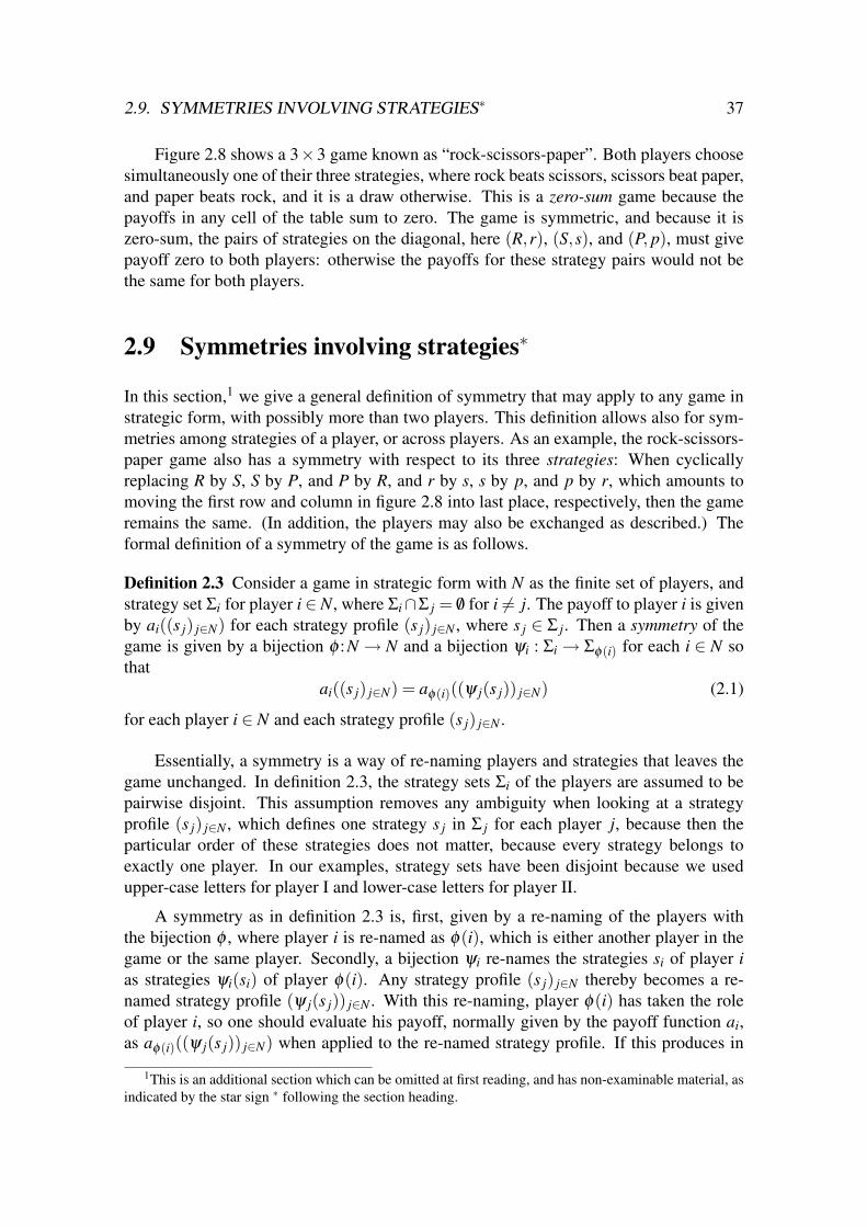
2.9. SYMMETRIES INVOLVING STRATEGIES∗ 37
Figure 2.8 shows a 3×3 game known as “rock-scissors-paper”. Both players choosesimultaneously one of their three strategies, where rock beats scissors, scissors beat paper,and paper beats rock, and it is a draw otherwise. This is a zero-sum game because thepayoffs in any cell of the table sum to zero. The game is symmetric, and because it iszero-sum, the pairs of strategies on the diagonal, here (R,r), (S,s), and (P, p), must givepayoff zero to both players: otherwise the payoffs for these strategy pairs would not bethe same for both players.
2.9 Symmetries involving strategies∗
In this section,1 we give a general definition of symmetry that may apply to any game instrategic form, with possibly more than two players. This definition allows also for sym-metries among strategies of a player, or across players. As an example, the rock-scissors-paper game also has a symmetry with respect to its three strategies: When cyclicallyreplacing R by S, S by P, and P by R, and r by s, s by p, and p by r, which amounts tomoving the first row and column in figure 2.8 into last place, respectively, then the gameremains the same. (In addition, the players may also be exchanged as described.) Theformal definition of a symmetry of the game is as follows.
Definition 2.3 Consider a game in strategic form with N as the finite set of players, andstrategy set Σi for player i ∈ N, where Σi∩Σ j = /0 for i 6= j. The payoff to player i is givenby ai((s j) j∈N) for each strategy profile (s j) j∈N , where s j ∈ Σ j. Then a symmetry of thegame is given by a bijection φ :N → N and a bijection ψi : Σi→ Σφ(i) for each i ∈ N sothat
ai((s j) j∈N) = aφ(i)((ψ j(s j)) j∈N) (2.1)
for each player i ∈ N and each strategy profile (s j) j∈N .
Essentially, a symmetry is a way of re-naming players and strategies that leaves thegame unchanged. In definition 2.3, the strategy sets Σi of the players are assumed to bepairwise disjoint. This assumption removes any ambiguity when looking at a strategyprofile (s j) j∈N , which defines one strategy s j in Σ j for each player j, because then theparticular order of these strategies does not matter, because every strategy belongs toexactly one player. In our examples, strategy sets have been disjoint because we usedupper-case letters for player I and lower-case letters for player II.
A symmetry as in definition 2.3 is, first, given by a re-naming of the players withthe bijection φ , where player i is re-named as φ(i), which is either another player in thegame or the same player. Secondly, a bijection ψi re-names the strategies si of player ias strategies ψi(si) of player φ(i). Any strategy profile (s j) j∈N thereby becomes a re-named strategy profile (ψ j(s j)) j∈N . With this re-naming, player φ(i) has taken the roleof player i, so one should evaluate his payoff, normally given by the payoff function ai,as aφ(i)((ψ j(s j)) j∈N) when applied to the re-named strategy profile. If this produces in
1This is an additional section which can be omitted at first reading, and has non-examinable material, asindicated by the star sign ∗ following the section heading.

38 CHAPTER 2. GAMES AS TREES AND IN STRATEGIC FORM
all cases the same payoffs, as stated in (2.1), then the re-naming has produced the samegame in strategic form, and is therefore called a symmetry of the game.
For two players, the reflection along the diagonal is obviously simpler to state andto observe. In this symmetry among the two players, with player set N = {I, II} andwith strategy sets ΣI and ΣII, we used φ(I) = II and thus φ(II) = I, and a single bijectionψI : ΣI→ΣII for re-naming the strategies, where ψII is the inverse of ψI. This last conditiondoes not have to apply in definition 2.3, which makes this definition more general.
@@@I
II
H
T
h t
1 −1
−1 1
−1 1
1 −1
Figure 2.9 The “matching pennies” game.
The game of “matching pennies” in figure 2.9 illustrates the greater generality of def-inition 2.3. This zero-sum game is played with two players that each have a penny, whichthe player can choose to show as heads or tails, which is the strategy H or T for player I,and h or t for player II. If the pennies match, for the strategy pairs (H,h) and (T, t), thenplayer II has to give her penny to player I; if they do not, for the strategy pairs (H, t) and(T,h), then player I loses his penny to player II. This game has an obvious symmetry instrategies where heads are exchanged with tails for both players, but where the playersare not re-named, so that φ is the identity function on the player set. However, the gamecannot be written so that it remains the same when reflected along the diagonal, becausethe diagonal payoffs would have to be zero, as in the rock-scissors-paper game, so it is notsymmetric among players in the sense of any of the earlier examples. Definition 2.3 doescapture the symmetry between the two players as follows (for example): φ exchanges Iand II, and ψI(H) = h, ψI(T ) = t, but ψII(h) = T , ψII(t) = H. That is, the sides of thepenny keep their meaning for player I when he is re-named as player II, but heads andtails change their role for player II. In effect, this exchanges the players’ preference formatching versus non-matching pennies, as required for the symmetry.
Please note: In the following discussion, when we call a game “symmetric”, wealways mean the simpler symmetry of a two-player game described in the previous sec-tion 2.8 that can be seen by reflecting the game along the diagonal.
2.10 Dominance and elimination of dominated strategies
This section discusses the concepts of strict and weak dominance, which apply to strate-gies and therefore to games in strategic form.

2.10. DOMINANCE AND ELIMINATION OF DOMINATED STRATEGIES 39
Definition 2.4 Consider a game in strategic form, and let s and t be two strategies of someplayer P of that game. Then s dominates (or strictly dominates) t if for any fixed strategiesof the other players, the payoff to player P when using s is higher than his payoff whenusing t. Strategy s weakly dominates t if for any fixed strategies of the other players, thepayoff to player P when using s is at least as high as when using t, and in at least one casestrictly higher.
In a two-player game, player P in definition 2.4 is either player I or player II. Forplayer I, his strategy s dominates t if row s of the payoffs to player I is in each componentlarger than row t. If one denotes the payoff to player I for row i and column j by a(i, j),then s dominates t if a(s, j) > a(t, j) for each strategy j of player II. Similarly, if thepayoff to player II is denoted by b(i, j), and s and t are two strategies of player II, whichare columns of the payoff table, then s dominates t if b(i,s) > b(i, t) for each strategy i ofplayer I.
In the prisoner’s dilemma game in figure 2.5, strategy D of player I dominates strat-egy C, because, with the notation of the preceding paragraph, a(D,c) = 3 > 2 = a(C,c)and a(D,d) = 1 > 0 = a(C,d). Because the game is symmetric, strategy d of player IIalso dominates c.
It would be inaccurate to define dominance by saying that a strategy s dominatesstrategy t if s is “always” better than t. This is only correct if “always” means “giventhe same strategies of the other players”. Even if s dominates t, it may happen that somepayoff when playing s is worse than some other payoff when playing t. For example,a(C,c) = 2 > 1 = a(D,d) in the prisoner’s dilemma game, so this is a case where thedominating strategy D gives a lower payoff than C. However, the strategy used by theother player is necessarily different in that case. When s dominates t, then strategy sis better than t when considering any arbitrary (but same) fixed strategies of the otherplayers.
Dominance is sometimes called strict dominance in order to distinguish it from weakdominance. Consider a two-player game with payoffs a(i, j) to player I and b(i, j) toplayer II when they play row i and column j. According to definition 2.4, strategy s ofplayer I weakly dominates t if a(s, j) ≥ a(t, j) for all j and a(s, j) > a(t, j) for at leastone column j. The latter condition ensures that if the two rows s and t of payoffs toplayer I are equal, s is not said to weakly dominate t (because for the same reason, t couldalso be said to dominate s). Similarly, if s and t are strategies of player II, then s weaklydominates t if the column s of payoffs b(i,s) to player II is in each component i at leastas large as column t, and strictly larger, with b(i,s) > b(i, t), in at least one row i. Anexample of such a strategy is l in figure 2.3(b), which is weakly dominated by r.
When a strategy s of player P dominates his strategy t, player P can always improvehis payoff by playing s rather than t. This follows from the way a game in strategic form isplayed, where the players choose their strategies simultaneously, and the game is playedonly once.2 Then player P may consider the strategies of the other players as fixed, and
2The game in strategic form is considered as a “one-shot” game. Many studies concern the possibleemergence of cooperation in the prisoner’s dilemma when the game is repeated, which is a different context.

40 CHAPTER 2. GAMES AS TREES AND IN STRATEGIC FORM
his own strategy choice cannot be observed and should not influence the choice of theothers, so he is better off playing s rather than t.
In consequence, one may study the game where all dominated strategies are elimi-nated. If some strategies are eliminated in this way, one then obtains a game that is simplerbecause some players have fewer strategies. In the prisoner’s dilemma game, eliminationof the dominated strategies C and c results in a game that has only one strategy per player,D for player I and d for player II. This strategy profile (D,d) may therefore be consideredas a “solution” of the game, a recommendation of a strategy for each player.
@@@I
II
T
B
l r
2 0
2 1
3 1
0 1
Figure 2.10 The “quality game”, with T and B as good or bad quality offered byplayer I, and l and r as buying or refusing to buy the product as strategiesof player II.
If one accepts that a player will never play a dominated strategy, one may eliminateit from the game and continue eliminating strategies that are dominated in the resultinggame. This is called iterated elimination of dominated strategies. If this process ends in aunique strategy profile, the game is said to be dominance solvable, with the final strategyprofile as its solution.
The “quality game” in figure 2.10 is a game that is dominance solvable in this way.The game is nearly identical to the prisoner’s dilemma game in figure 2.5, except for thepayoff to player II for the top right cell of the table, which is changed from 3 to 1. Thegame may describe the situation of, say, player I as a restaurant owner, who can providefood of good quality (strategy T ) or bad quality (B), and a potential customer, player II,who may decide to eat there (l) or not (r). The customer prefers l to r only if the qualityis good. However, whatever player II does, player I is better off by choosing B, whichtherefore dominates T . After eliminating T from the game, player II’s two strategies l andr remain, but in this smaller game r dominates l, and l is therefore eliminated in a seconditeration. The resulting strategy pair is (B,r).
When eliminating dominated strategies, the order of elimination does not matter,because if s dominates t, then s still dominates t in the game where some strategies (otherthan t) are eliminated. In contrast, when eliminating weakly dominated strategies, theorder of elimination may matter. Moreover, a weakly dominated strategy, such as strategyl of player II in figure 2.3, may be just as good as the strategy that weakly dominates it,if the other player chooses some strategy, like T in figure 2.3, where the two strategieshave equal payoff. Hence, there are no strong reasons for eliminating a weakly dominatedstrategy in the first place.

2.11. NASH EQUILIBRIUM 41
⇒ Exercise 2.5 on page 54 studies weakly dominated strategies, and what can happenwhen these are eliminated. You can answer this exercise except for (d) which youshould do after having understood the concept of Nash equilibrium, treated in thenext section.
2.11 Nash equilibrium
Not every game is dominance solvable, as the games of chicken and the battle of sexesdemonstrate. The central concept of non-cooperative game theory is that of equilibrium,often called Nash equilibrium after John Nash, who introduced this concept in 1950 forgeneral games in strategic form (the equivalent concept for zero-sum games was consid-ered earlier). An equilibrium is a strategy profile where each player’s strategy is a “bestresponse” to the remaining strategies.
Definition 2.5 Consider a game in strategic form and a strategy profile given by a strategys j for each player j. Then for player i, his strategy si is a best response to the strategiesof the remaining players if no other strategy gives player i a higher payoff, when thestrategies of the other players are unchanged. An equilibrium of the game, also calledNash equilibrium, is a strategy profile where the strategy of each player is a best responseto the other strategies.
In other words, a Nash equilibrium is a strategy profile so that no player can gain bychanging his strategy unilaterally, that is, with the remaining strategies kept fixed.
@@@I
II
T
B
l r
2 0
2 1
3 1
0 1↓ ↓
←
→
(a)@
@@I
II
T
B
l r
2 0
2 1
3 1
0 1
(b)
Figure 2.11 Indicating best responses in the quality game with arrows (a), or by puttingbest response payoffs in boxes (b).
Figure 2.11(a) shows the quality game of figure 2.10 where the best responses areindicated with arrows: The downward arrow on the left shows that if player II plays herleft strategy l, then player I has best response B; the downward arrow on the right showsthat the best response to r is also B; the leftward arrow at the top shows that player II’sbest response to T is l, and the rightward arrow at the bottom that the best response to Bis r.
This works well for 2× 2 games, and shows that a Nash equilibrium is where thearrows “flow together”. For the quality game, player I’s arrows both point downwards,

42 CHAPTER 2. GAMES AS TREES AND IN STRATEGIC FORM
which shows that B dominates T , and the bottom arrow points right, so that starting fromany cell and following the arrows, one arrives at the equilibrium (B,r).
In figure 2.11(b), best responses are indicated by boxes drawn around the payoffs foreach strategy that is a best response. For player I, a best response is considered against astrategy of player II. That strategy is a column of the game, so the best response payoffis the maximum of each column (which may occur more than once) of the payoffs ofplayer I. Similarly, a best response payoff for player II is the maximum in each row of thepayoffs to player II. Unlike arrows, putting best response payoffs into boxes can be doneeasily even when a player has more than two strategies. A Nash equilibrium is then givenby a cell of the table where both payoffs are boxed.
@@@I
II
A
C
a c
0 2
0 1
1 1
2 1
(a)@
@@I
II
C
S
c s
1 0
2 0
0 2
0 1
(b)
Figure 2.12 Best responses and Nash equilibria in the game of chicken (a), and in thebattle of sexes game (b).
The game of chicken in figure 2.12(a) has two equilibria, (A,c) and (a,C). If a gameis symmetric, like in this case, then an equilibrium is symmetric if it does not change underthe symmetry (that is, when exchanging the two players). Neither of the two equilibria(A,c) and (a,C) is symmetric, but they map to each other under the symmetry (any non-symmetric equilibrium must have a symmetric counterpart; only symmetric equilibriamap to themselves).
As figure 2.12(b) shows, the battle of sexes game has two Nash equilibria, (C,c)and (S,s). (When writing the battle of sexes game symmetrically as in figure 2.7(b), itsequilibria are not symmetric either.) The prisoner’s dilemma game has one equilibrium(D,d), which is symmetric.
It is clear that a dominated strategy is never a best response, and hence cannot bepart of an equilibrium. Consequently, one can eliminate any dominated strategy from agame, and not lose any equilibrium. Moreover, this elimination cannot create additionalequilibria because any best response in the absence of a dominated strategy remains abest response when adding the dominated strategy back to the game. By repeating thisargument when considering the iterated elimination of dominated strategies, we obtainthe following proposition.
Proposition 2.6 If a game in strategic form is dominance solvable, its solution is the onlyNash equilibrium of the game.
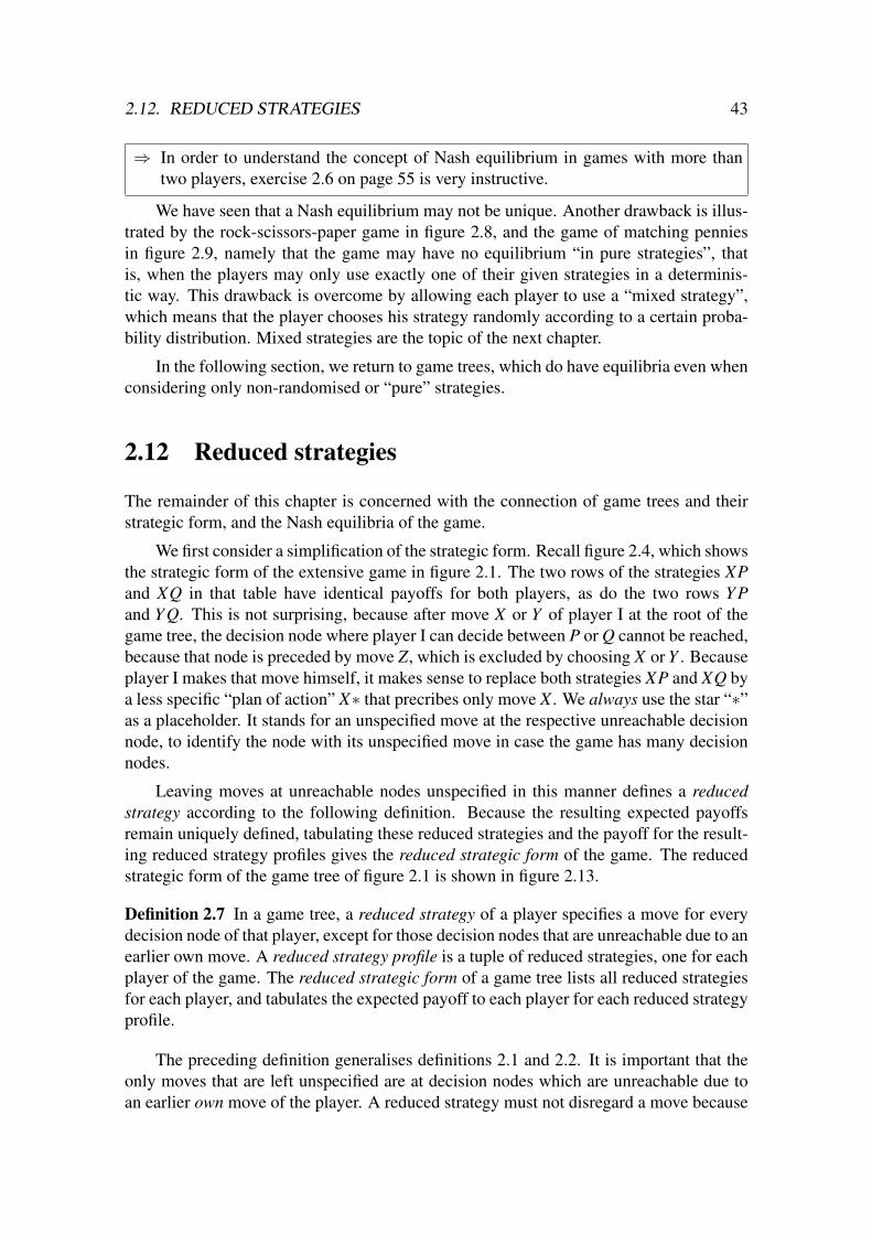
2.12. REDUCED STRATEGIES 43
⇒ In order to understand the concept of Nash equilibrium in games with more thantwo players, exercise 2.6 on page 55 is very instructive.
We have seen that a Nash equilibrium may not be unique. Another drawback is illus-trated by the rock-scissors-paper game in figure 2.8, and the game of matching penniesin figure 2.9, namely that the game may have no equilibrium “in pure strategies”, thatis, when the players may only use exactly one of their given strategies in a determinis-tic way. This drawback is overcome by allowing each player to use a “mixed strategy”,which means that the player chooses his strategy randomly according to a certain proba-bility distribution. Mixed strategies are the topic of the next chapter.
In the following section, we return to game trees, which do have equilibria even whenconsidering only non-randomised or “pure” strategies.
2.12 Reduced strategies
The remainder of this chapter is concerned with the connection of game trees and theirstrategic form, and the Nash equilibria of the game.
We first consider a simplification of the strategic form. Recall figure 2.4, which showsthe strategic form of the extensive game in figure 2.1. The two rows of the strategies XPand XQ in that table have identical payoffs for both players, as do the two rows Y Pand Y Q. This is not surprising, because after move X or Y of player I at the root of thegame tree, the decision node where player I can decide between P or Q cannot be reached,because that node is preceded by move Z, which is excluded by choosing X or Y . Becauseplayer I makes that move himself, it makes sense to replace both strategies XP and XQ bya less specific “plan of action” X∗ that precribes only move X . We always use the star “∗”as a placeholder. It stands for an unspecified move at the respective unreachable decisionnode, to identify the node with its unspecified move in case the game has many decisionnodes.
Leaving moves at unreachable nodes unspecified in this manner defines a reducedstrategy according to the following definition. Because the resulting expected payoffsremain uniquely defined, tabulating these reduced strategies and the payoff for the result-ing reduced strategy profiles gives the reduced strategic form of the game. The reducedstrategic form of the game tree of figure 2.1 is shown in figure 2.13.
Definition 2.7 In a game tree, a reduced strategy of a player specifies a move for everydecision node of that player, except for those decision nodes that are unreachable due to anearlier own move. A reduced strategy profile is a tuple of reduced strategies, one for eachplayer of the game. The reduced strategic form of a game tree lists all reduced strategiesfor each player, and tabulates the expected payoff to each player for each reduced strategyprofile.
The preceding definition generalises definitions 2.1 and 2.2. It is important that theonly moves that are left unspecified are at decision nodes which are unreachable due toan earlier own move of the player. A reduced strategy must not disregard a move because

44 CHAPTER 2. GAMES AS TREES AND IN STRATEGIC FORM
@@@I
II
X∗
Y∗
ZP
ZQ
ad ae bd be cd ce
3 3 2 2 4 4
4 4 5 5 5 5
2 2 2 2 2 2
3 3 3 3 3 3
1 0 1 0 1 0
3 5 3 5 3 5
1 4 1 4 1 4
3 2 3 2 3 2
Figure 2.13 Reduced strategic form of the extensive game in figure 2.1. The star ∗stands for an arbitrary move at the second decision node of player I, whichis not reachable after move X or Y .
another player may not move there, because that possibility cannot be excluded by lookingonly at the player’s own moves. In the game tree in figure 2.1, for example, no reductionis possible for the strategies of player II, because neither of her moves at one decisionnode precludes a move at her other decision node. Therefore, the reduced strategies ofplayer II in that game are the same as her (unreduced, original) strategies.
In definition 2.7, reduced strategies are defined without any reference to payoffs, onlyby looking at the structure of the game tree. One could derive the reduced strategic formin figure 2.13 from the strategic form in figure 2.4 by identifying the strategies that haveidentical payoffs for both players and replacing them by a single reduced strategy. Someauthors define the reduced strategic form in terms of this elimination of duplicate strate-gies in the strategic form. (Sometimes, dominated strategies are also eliminated whendefining the reduced strategic form.) We define the reduced strategic form without anyreference to payoffs because strategies may have identical payoffs by accident, due tospecial payoffs at the leaves of the game (this does not occur in generic games). More-over, we prefer that reduced strategies refer to the structure of the game tree, not to somerelationship of the payoffs, which is a different aspect of the game.
Strategies are combinations of moves, so for every additional decision node of aplayer, each move at that node can be combined with move combinations already consid-ered. The number of move combinations therefore grows exponentially with the numberof decision nodes of the player, because it is the product of the numbers of moves at eachnode. In the game in figure 2.14, for example, where m possible initial moves of player Iare followed each time by two possible moves of player II, the number of strategies ofplayer II is 2m. Moreover, this is also the number of reduced strategies of player II be-cause no reduction is possible. This shows that even the reduced strategic form can beexponentially large in the size of the game tree. If a player’s move is preceded by an own

2.13. SUBGAME PERFECT NASH EQUILIBRIUM (SPNE) 45
����
������
����������������������
����
����
I
II
rl
C C
l r1 1
II
l r2 2
II
C m21
mm
Figure 2.14 Extensive game with m moves C1, . . . ,Cm of player I at the root of the gametree. To each move Ci, player II may respond with two possible moves li orri. Player II has 2m strategies.
earlier move, the reduced strategic form is smaller because then that move can be leftunspecified if the preceding own move is not made.
⇒ Exercise 2.4 on page 54 tests your understanding of reduced strategies.
In the reduced strategic form, a Nash equilibrium is defined, as in definition 2.5, as aprofile of reduced strategies, each of which is a best response to the others.
In this context, we will for brevity sometimes refer to reduced strategies simply as“strategies”. This is justified because, when looking at the reduced strategic form, theconcepts of dominance and equilibrium can be applied directly to the reduced strategicform, for example to the table defining a two-player game. Then “strategy” means simplya row or column of that table. The term “reduced strategy” is only relevant when referringto the extensive form.
The Nash equilibria in figure 2.13 are identified as those pairs of (reduced) strategiesthat are best responses to each other, with both payoffs surrounded by a box in the respec-tive cell of the table. These Nash equilibria in reduced strategies are (X∗,bd), (X∗,cd),(X∗,ce), and (Y∗,bd).
⇒ You are now in a position answer (b)–(e) of exercise 2.1 on page 52.
2.13 Subgame perfect Nash equilibrium (SPNE)
In this section, we consider the relationship between Nash equilibria of games in extensiveform and backward induction.
The 2×2 game in figure 2.3(b) has two Nash equilibria, (T, l) and (B,r). The strategypair (B,r) is also obtained, uniquely, by backward induction. We will prove shortly thatbackward induction always defines a Nash equilibrium.
The equilibrium (T, l) in figure 2.3(b) is not obtained by backward induction, becauseit prescribes the non-optimal move l for player II at her only decision node. Moreover, lis a weakly dominated strategy. Nevertheless, this is a Nash equilibrium because T is thebest response to l, and, moreover, l is a best response to T because against T , the payoff

46 CHAPTER 2. GAMES AS TREES AND IN STRATEGIC FORM
to player II is no worse than when choosing r. This can also be seen when considering thegame tree in figure 2.3(a): Move l is a best response to T because player II never has tomake that move when player I chooses T , so player II’s move does not affect her payoff,and she is indifferent between l and r. On the other hand, only when she makes move lis it optimal for player I to respond by choosing T , because against r player I would getmore by choosing B.
The game in figure 2.3(a) is also called a “threat game” because it has a Nash equi-librium (T, l) where player II “threatens” to make the move l that is bad for both players,against which player I chooses T , which is then advantageous for player II compared tothe backward induction outcome when the players choose (B,r). The threat works onlybecause player II never has to execute it, given that player I acts rationally and chooses T .
The concept of Nash equilibrium is based on the strategic form because it applies to astrategy profile. When applied to a game tree, the strategies in that profile are assumed tobe chosen by the players before the game starts, and the concept of best response appliesto this given expectation of what the other players will do.
With the game tree as the given specification of the game, it is often desirable to keepits sequential interpretation. The strategies chosen by the players should therefore alsoexpress some “sequential rationality” as expressed by backward induction. That is, themoves in a strategy profile should be optimal for any part of the game, including subtreesthat cannot be reached due to earlier moves, possibly of other players, like the tree startingat the decision node of player II in the threat game in figure 2.3(a).
In a game tree, a subgame is any subtree of the game, given by a node of the tree asthe root of the subtree and all its descendants. (Note: This definition of a subgame appliesonly to games with perfect information, which are the game trees considered so far. Inextensive games with imperfect information, which we consider later, the subtree is a sub-game only if all players know that they are in that subtree.) A strategy profile that definesa Nash equilibrium for every subgame is called a subgame perfect Nash equilibrium orSPNE.
⇒ You can now answer the final question (e) of exercise 2.1 on page 52, and exer-cise 2.2 on page 53.
Theorem 2.8 Backward induction defines an SPNE.
Proof. Recall the process of backward induction: Starting with the nodes closest to theleaves, consider a decision node u, say, with the assumption that all moves after u havealready been selected. Among the moves at u, select a move that maximises the expectedpayoff to the player that moves at u. (Expected payoffs must be regarded if there arechance moves after u.) In that manner, a move is selected for every decision node, whichdetermines an entire strategy profile.
We prove the theorem inductively: Consider a non-terminal node u of the game tree,which may be a decision node (as in the backward induction process), or a chance node.Suppose that the moves at u are c1,c2, . . . ,ck, which lead to subtrees T1,T2, . . . ,Tk of thegame tree, and assume, as inductive hypothesis, that the moves selected so far define an

2.13. SUBGAME PERFECT NASH EQUILIBRIUM (SPNE) 47
SPNE in each of these trees. (As the “base case” of the induction, this is certainly true ifeach of T1,T2, . . . ,Tk is just a leaf of the tree, so that u is a “last” decision node consideredfirst in the backward induction process.) The induction step is completed if one showsthat, by selecting the move at u, one obtains an SPNE for the subgame with root u.
First, suppose that u is a chance node, so that the next node is chosen according to thefixed probabilities specified in the game tree. Then backward induction does not selecta move for u, and the inductive step holds trivially: For every player, the payoff in thesubgame starting at u is the expectation of the payoffs for each subgame Ti (weightedwith the probability for move ci), and if a player could improve on that payoff, she wouldhave to do so by changing her moves within at least one subtree Ti, which, by inductivehypothesis, she cannot.
Secondly, suppose that u is a decision node, and consider a player other than theplayer to move at u. Again, for that player, the moves in the subgame starting at u arecompletely specified, and, irrespective of what move is selected for u, she cannot im-prove her payoff because that would mean she could improve her payoff already in somesubtree Ti.
Finally, consider the player to move at u. Backward induction selects a move for uthat is best for that player, given the remaining moves. Suppose the player could improvehis payoff by choosing some move ci and additionally change his moves in the subtree Ti.But the resulting improved payoff would only be the improved payoff in Ti, that is, theplayer could already get a better payoff in Ti itself, contradicting the inductive assumptionthat the moves selected so far defined an SPNE for Ti. This completes the induction.
This theorem has two important consequences. In backward induction, each movecan be chosen deterministically, so that backward induction determines a profile of purestrategies. Theorem 2.8 therefore implies that game trees have Nash equilibria, and it isnot necessary to consider randomised strategies. Secondly, subgame perfect Nash equi-libria exist. For game trees, we can use “SPNE” synonymously with “strategy profileobtained by backward induction”.
Corollary 2.9 Every game tree with perfect information has a pure-strategy Nash equi-librium.
Corollary 2.10 Every game tree has an SPNE.
In order to describe an SPNE, it is important to consider unreduced (that is, fullyspecified) strategies. Recall that in the game in figure 2.1, the SPNE are (XQ,bd),(XQ,cd), and (Y Q,bd). The reduced strategic form of the game in figure 2.13 showsthe Nash equilibria (X∗,bd), (X∗,cd), and (Y∗,bd). However, we cannot call any ofthese an SPNE because they leave the second move of player I unspecified, as indicatedby the ∗ symbol. In this case, replacing ∗ by Q results in all cases in an SPNE. The fullstrategies are necessary to determine if they define a Nash equilibrium in every subgame.As seen in figure 2.13, the game has, in addition, the Nash equilibrium (X∗,ce). This isnot subgame perfect because it prescribes the move e, which is not part of a Nash equi-librium in the subgame starting with the decision node where player II chooses between

48 CHAPTER 2. GAMES AS TREES AND IN STRATEGIC FORM
d and e: When replacing ∗ by P, this would not be the best response by player I to e inthat subgame, and when replacing ∗ by Q, player II’s best response would not be e. Thisproperty can only be seen in the game tree, not even in the unreduced strategic form infigure 2.4, because it concerns an unreached part of the game tree due to the earlier moveX of player I.
⇒ For understanding subgame perfection, exercise 2.3 on page 54 is very instructive.Exercise 2.7 on page 56 studies a three-player game.
2.14 Commitment games
The main difference between game trees and games in strategic form is that in a gametree, players act sequentially, being aware of the previous moves of the other players.In contrast, players in a game in strategic form move simultaneously. The differencebetween these two descriptions becomes striking when changing a two-player game instrategic form to a commitment game, as described in this section.
We start with a two-player game in strategic form, say an m× n game. The corre-sponding commitment game is an extensive game with perfect information. One of theplayers (we always choose player I) moves first, by choosing one of his m strategies.Then, unlike in the strategic form, player II is informed about the move of player I. Foreach move of player I, the possible moves of player II are the n strategies of the originalstrategic form game, with resulting payoffs to both players as specified in that game.
����
����
����II
T B
I
II
2 02 1
r
3 10 1
rl lTT B B
@@I
II
T
B
lT lB lT rB rT lB rT rB
2 2 0 0
2 2 1 1
3 1 3 1
0 1 0 1
(b)(a)
Figure 2.15 The extensive game (a) is the commitment game of the quality game infigure 2.10. Player I moves first, and player II can react to that choice.The arrows show the backward induction outcome. Its strategic form withbest-response payoffs is shown in (b).
An example is figure 2.15, which is the commitment game for the quality game infigure 2.10. The original strategies T and B of player I become his moves T and B. Ingeneral, if player I has m strategies in the given game, he also has m strategies in thecommitment game. In the commitment game, each strategy l or r of player II becomes amove, which depends on the preceding move of player I, so we call them lT and rT whenfollowing move T , and lB and rB when following move B. In general, when player I hasm moves in the commitment game and player II has n responses, then each combination

2.14. COMMITMENT GAMES 49
of moves defines a pure strategy of player II, so she has nm strategies in the commitmentgame. Figure 2.15(b) shows the resulting strategic form of the commitment game in theexample. It shows that the given game and the commitment game are very different.
We then look for subgame perfect equilibria of the commitment game, that is, applybackward induction, which we can do because the game has perfect information. Fig-ure 2.15(a) shows that the resulting unique SPNE is (T, lT rB), which means that (goingbackwards) player II, when offered high quality T , chooses lT , and rB when offered lowquality. In consequence, player I will then choose T because that gives him the higherpayoff 2 rather than just 1 with B. Note that it is important that player I has the power tocommit to T and cannot change later back to B after seeing that player II chose l; with-out that commitment power, the game would not be accurately reflected by the extensivegame as described.
The commitment game in figure 2.15 also demonstrates the difference between anequilibrium, which is a strategy profile, and the equilibrium path, which is describedby the moves that are actually played in the game when players use their equilibriumstrategies. If the game has no chance moves, the equilibrium path is just a certain path inthe game tree. In contrast, a strategy profile defines a move in every part of the game tree.Here, the SPNE (T, lT rB) specifies moves lT and rB for both decision points of player II.Player I chooses T , and then only lT is played. The equilibrium path is then given bymove T followed by move lT . However, it is not sufficient to simply call this equilibrium(T, lT ) or (T, l), because player II’s move rB must be specified to know that T is player I’sbest response.
We only consider SPNE when analysing commitment games. For example, the Nashequilibrium (B,r) of the original quality game in figure 2.10 can also be found in fig-ure 2.15, where player II always chooses the move r corresponding to her equilibriumstrategy in the original game, which is the strategy rT rB in the commitment game. Thisdefines the Nash equilibrium (B,rT rB) in the commitment game, because B is a bestresponse to rT rB, and rT rB is a best response to B (which clearly holds as a general ar-gument, starting with any Nash equilibrium of the original game). However, this Nashequilibrium of the commitment game is not subgame perfect, because it prescribes thesuboptimal move rT off the equilibrium path; this does not affect the Nash equilibriumproperty because T is not chosen by player I. In order to compare a strategic-form gamewith its commitment game in an interesting way, we consider only SPNE of the commit-ment game.
A practical application of a game-theoretic analysis may be to reveal the potentialeffects of changing the “rules” of the game. This is illustrated by changing the qualitygame to its commitment version.
⇒ This is a good point to try exercise 2.8 on page 56.
Games in strategic form, when converted to a commitment game, typically have afirst-mover advantage. A player in a game becomes a first mover or “leader” when hecan commit to a strategy as described, that is, choose a strategy irrevocably and informthe other players about it; this is a change of the “rules of the game”. The first-moveradvantage states that a player who can become a leader is not worse off than in the original

50 CHAPTER 2. GAMES AS TREES AND IN STRATEGIC FORM
game where the players act simultaneously. In other words, if one of the players has thepower to commit, he or she should do so.
This statement must be interpreted carefully. For example, if more than one playerhas the power to commit, then it is not necessarily best to go first. For example, considerchanging the game in figure 2.10 so that player II can commit to her strategy, and player Imoves second. Then player I will always respond by choosing B because this is hisdominant strategy in figure 2.10. Backward induction would then amount to player IIchoosing l, and player I choosing BlBr, with the low payoff 1 to both. Then player IIis not worse off than in the simultaneous-choice game, as asserted by the first-moveradvantage, but does not gain anything either. In contrast, making player I the first moveras in figure 2.15 is beneficial to both.
The first-mover advantage is also known as Stackelberg leadership, after the econ-omist Heinrich von Stackelberg, who formulated this concept for the structure of marketsin 1934. The classic application is to the duopoly model by Cournot, which dates back to1838.
@@@I
II
H
M
L
N
h m l n
0 12 18 36
0 8 9 0
8 16 20 32
12 16 15 0
9 15 18 27
18 20 18 0
0 0 0 0
36 32 27 0
Figure 2.16 Duopoly game between two chip manufacturers who can decide betweenhigh, medium, low, or no production, denoted by H,M,L,N for player Iand h,m, l,n for player II. Payoffs denote profits in millions of dollars.
As an example, suppose that the market for a certain type of memory chip is domi-nated by two producers. The players can choose to produce a certain quantity of chips, sayeither high, medium, low, or none at all, denoted by H,M,L,N for player I and h,m, l,n forplayer II. The market price of the memory chips decreases with increasing total quantityproduced by both companies. In particular, if both choose a high quantity of production,the price collapses so that profits drop to zero. The players know how increased produc-tion lowers the chip price and their profits. Figure 2.16 shows the game in strategic form,where both players choose their output level simultaneously. The symmetric payoffs arederived from Cournot’s model, explained below.
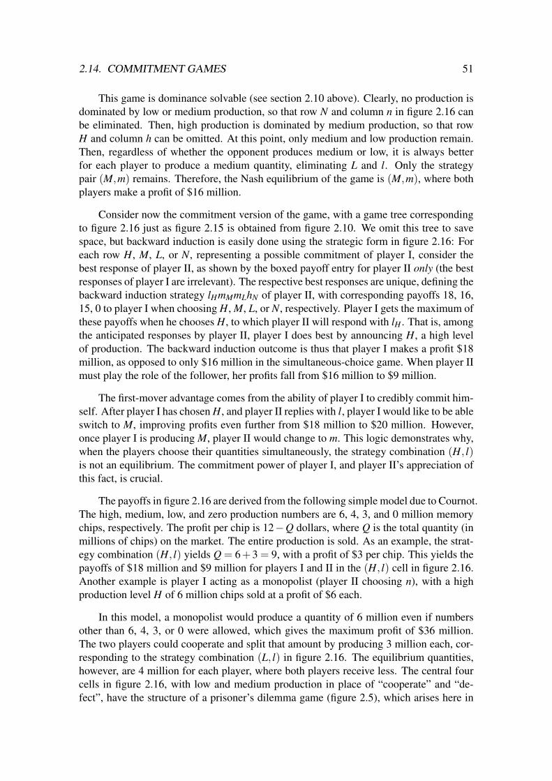
2.14. COMMITMENT GAMES 51
This game is dominance solvable (see section 2.10 above). Clearly, no production isdominated by low or medium production, so that row N and column n in figure 2.16 canbe eliminated. Then, high production is dominated by medium production, so that rowH and column h can be omitted. At this point, only medium and low production remain.Then, regardless of whether the opponent produces medium or low, it is always betterfor each player to produce a medium quantity, eliminating L and l. Only the strategypair (M,m) remains. Therefore, the Nash equilibrium of the game is (M,m), where bothplayers make a profit of $16 million.
Consider now the commitment version of the game, with a game tree correspondingto figure 2.16 just as figure 2.15 is obtained from figure 2.10. We omit this tree to savespace, but backward induction is easily done using the strategic form in figure 2.16: Foreach row H, M, L, or N, representing a possible commitment of player I, consider thebest response of player II, as shown by the boxed payoff entry for player II only (the bestresponses of player I are irrelevant). The respective best responses are unique, defining thebackward induction strategy lHmMmLhN of player II, with corresponding payoffs 18, 16,15, 0 to player I when choosing H, M, L, or N, respectively. Player I gets the maximum ofthese payoffs when he chooses H, to which player II will respond with lH . That is, amongthe anticipated responses by player II, player I does best by announcing H, a high levelof production. The backward induction outcome is thus that player I makes a profit $18million, as opposed to only $16 million in the simultaneous-choice game. When player IImust play the role of the follower, her profits fall from $16 million to $9 million.
The first-mover advantage comes from the ability of player I to credibly commit him-self. After player I has chosen H, and player II replies with l, player I would like to be ableswitch to M, improving profits even further from $18 million to $20 million. However,once player I is producing M, player II would change to m. This logic demonstrates why,when the players choose their quantities simultaneously, the strategy combination (H, l)is not an equilibrium. The commitment power of player I, and player II’s appreciation ofthis fact, is crucial.
The payoffs in figure 2.16 are derived from the following simple model due to Cournot.The high, medium, low, and zero production numbers are 6, 4, 3, and 0 million memorychips, respectively. The profit per chip is 12−Q dollars, where Q is the total quantity (inmillions of chips) on the market. The entire production is sold. As an example, the strat-egy combination (H, l) yields Q = 6+3 = 9, with a profit of $3 per chip. This yields thepayoffs of $18 million and $9 million for players I and II in the (H, l) cell in figure 2.16.Another example is player I acting as a monopolist (player II choosing n), with a highproduction level H of 6 million chips sold at a profit of $6 each.
In this model, a monopolist would produce a quantity of 6 million even if numbersother than 6, 4, 3, or 0 were allowed, which gives the maximum profit of $36 million.The two players could cooperate and split that amount by producing 3 million each, cor-responding to the strategy combination (L, l) in figure 2.16. The equilibrium quantities,however, are 4 million for each player, where both players receive less. The central fourcells in figure 2.16, with low and medium production in place of “cooperate” and “de-fect”, have the structure of a prisoner’s dilemma game (figure 2.5), which arises here in

52 CHAPTER 2. GAMES AS TREES AND IN STRATEGIC FORM
a natural economic context. The optimal commitment of a first mover is to produce aquantity of 6 million, with the follower choosing 3 million.
These numbers, and the equilibrium (“Cournot”) quantity of 4 million, apply evenwhen arbitrary quantities are allowed. That is, suppose x and y are the quantities ofproduction for player I and player II, respectively. The payoffs a(x,y) to player I andb(x,y) to player II are defined as
a(x,y) = x · (12− x− y),b(x,y) = y · (12− x− y). (2.2)
Then it is easy to see that player I’s best response x(y) to y is given by 6− y/2, andplayer II’s best response y(x) to x is given by 6−x/2. The pair of linear equations x(y) = xand y(x) = y has the solution x = y = 4, which is the above Nash equilibrium (M,m)of figure 2.16. In the commitment game, player I maximises his payoff, assuming theunique best response y(x) of player II in the SPNE, by maximising a(x,y(x)), which isx · (12− x−6 + x/2) = x · (12− x)/2. That maximum is given for x = 6, which happensto be the strategy H (high production) in figure 2.16. The best response of player II to thatcommitment is 6−6/2 = 3, which we have named strategy l for low production.
⇒ Exercise 2.9 on page 57 studies a game with infinite strategy sets like (2.2), andmakes interesting observations, in particular in (d), concerning the payoffs to thetwo players in the commitment game compared to the original simultaneous game.
2.15 Exercises for chapter 2
Exercises 2.1 and 2.2 ask you to apply the main concepts of this chapter to a simple gametree. A more detailed study of the concept of SPNE is exercise 2.3. Exercise 2.4 is oncounting strategies and reduced strategies. Exercise 2.5 shows that iterated eliminationof weakly dominated strategies is a problematic concept. Exercises 2.6 and 2.7 concernthree-player games, which are very important to understand because the concepts of dom-inance and equilibrium require to keep the strategies of all other players fixed; this is notlike just having another player in a two-player game. Exercise 2.8 is an instructive exer-cise on commitment games. Exercise 2.9 studies commitment games where in the originalgame both players have infinitely many strategies.
Exercise 2.1 Consider the following game tree. At a leaf, the top payoffs are for player I,the bottom payoffs are for player II.

2.15. EXERCISES FOR CHAPTER 2 53
����
����
����
����
����
I
IIII
I I102
93
92
84
111
L R
AB
C D E
barl
4 302
(a) What is the number of strategies of player I and of player II?
(b) How many reduced strategies do they have?
(c) Give the reduced strategic form of the game.
(d) What are the Nash equilibria of the game in reduced strategies?
(e) What are the subgame perfect Nash equilibria of the game?
Exercise 2.2 Consider the game tree in figure 2.17. At a leaf, the top payoff is for player I,the bottom payoff for player II.
•I@
@@
@@
@
¡¡
¡¡
¡¡
L R
•IIAAAAAA
¢¢
¢¢
¢¢
a b
• IIAAAAAA
¢¢
¢¢
¢¢
c d
• IAAAAAA
¢¢
¢¢
¢¢
S T52
31
41
12
03
Figure 2.17 Game tree for exercise 2.2.
(a) What is the number of strategies of player I and of player II? How many reducedstrategies does each of the players have?
(b) Give the reduced strategic form of the game.
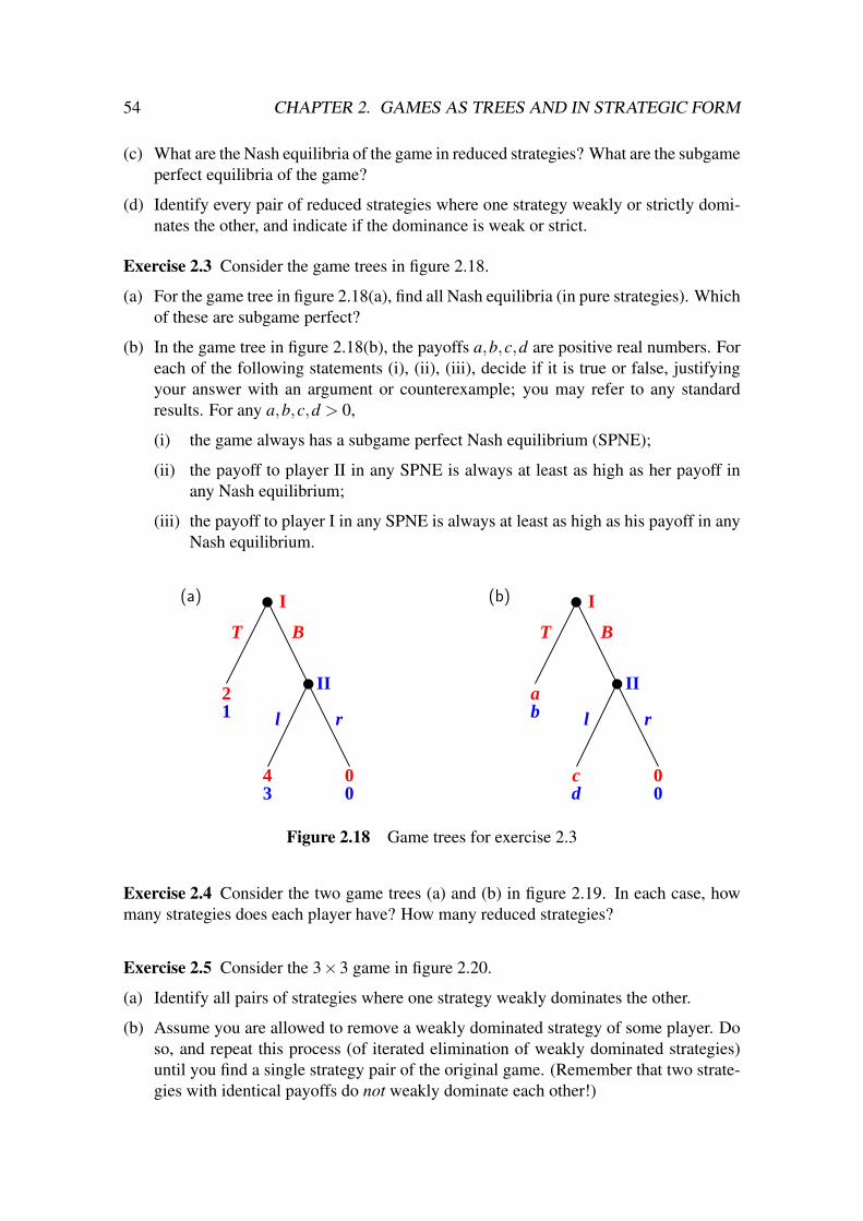
54 CHAPTER 2. GAMES AS TREES AND IN STRATEGIC FORM
(c) What are the Nash equilibria of the game in reduced strategies? What are the subgameperfect equilibria of the game?
(d) Identify every pair of reduced strategies where one strategy weakly or strictly domi-nates the other, and indicate if the dominance is weak or strict.
Exercise 2.3 Consider the game trees in figure 2.18.
(a) For the game tree in figure 2.18(a), find all Nash equilibria (in pure strategies). Whichof these are subgame perfect?
(b) In the game tree in figure 2.18(b), the payoffs a,b,c,d are positive real numbers. Foreach of the following statements (i), (ii), (iii), decide if it is true or false, justifyingyour answer with an argument or counterexample; you may refer to any standardresults. For any a,b,c,d > 0,
(i) the game always has a subgame perfect Nash equilibrium (SPNE);
(ii) the payoff to player II in any SPNE is always at least as high as her payoff inany Nash equilibrium;
(iii) the payoff to player I in any SPNE is always at least as high as his payoff in anyNash equilibrium.
(a)
T B
I
II
l r
00
2
43
1
(b)
T B
I
II
l r
00
ab
cd
Figure 2.18 Game trees for exercise 2.3
Exercise 2.4 Consider the two game trees (a) and (b) in figure 2.19. In each case, howmany strategies does each player have? How many reduced strategies?
Exercise 2.5 Consider the 3×3 game in figure 2.20.
(a) Identify all pairs of strategies where one strategy weakly dominates the other.
(b) Assume you are allowed to remove a weakly dominated strategy of some player. Doso, and repeat this process (of iterated elimination of weakly dominated strategies)until you find a single strategy pair of the original game. (Remember that two strate-gies with identical payoffs do not weakly dominate each other!)
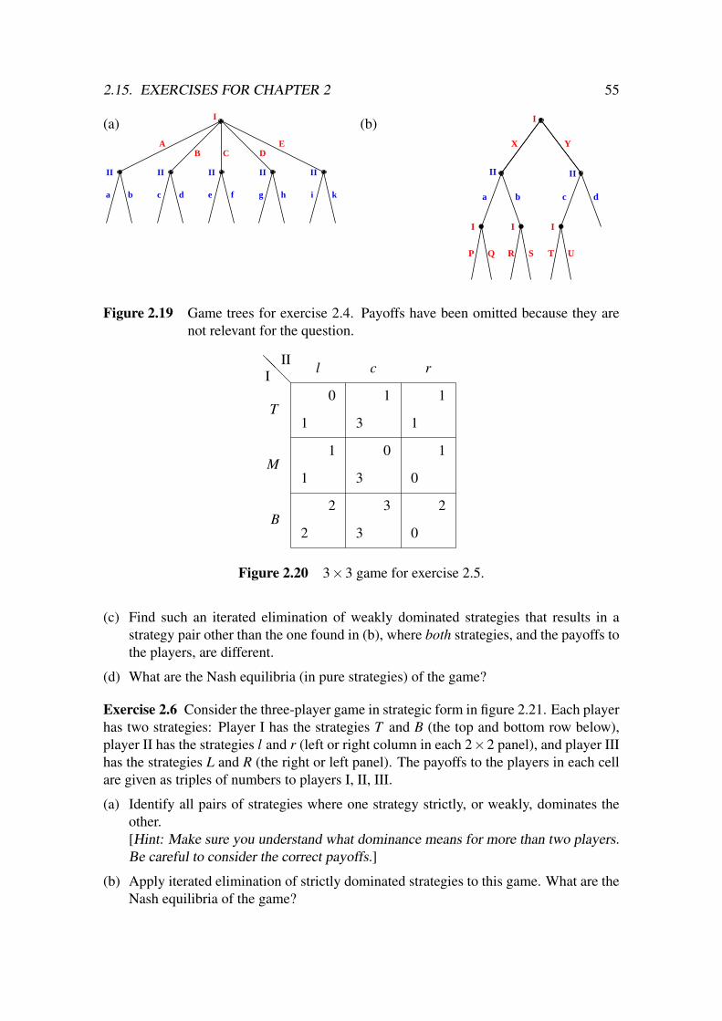
2.15. EXERCISES FOR CHAPTER 2 55
(a) (b)
����
��������
����
����
����
����II
a b
I
CA E
DB
II
c d
II
e f
II
g h
II
i k
����
����
����
P Q
I
R S
I
T U
I
I
X Y
II II
c dba
Figure 2.19 Game trees for exercise 2.4. Payoffs have been omitted because they arenot relevant for the question.
@@@I
II
T
M
B
l c r
1 3 1
0 1 1
1 3 0
1 0 1
2 3 0
2 3 2
Figure 2.20 3×3 game for exercise 2.5.
(c) Find such an iterated elimination of weakly dominated strategies that results in astrategy pair other than the one found in (b), where both strategies, and the payoffs tothe players, are different.
(d) What are the Nash equilibria (in pure strategies) of the game?
Exercise 2.6 Consider the three-player game in strategic form in figure 2.21. Each playerhas two strategies: Player I has the strategies T and B (the top and bottom row below),player II has the strategies l and r (left or right column in each 2×2 panel), and player IIIhas the strategies L and R (the right or left panel). The payoffs to the players in each cellare given as triples of numbers to players I, II, III.
(a) Identify all pairs of strategies where one strategy strictly, or weakly, dominates theother.[Hint: Make sure you understand what dominance means for more than two players.Be careful to consider the correct payoffs.]
(b) Apply iterated elimination of strictly dominated strategies to this game. What are theNash equilibria of the game?
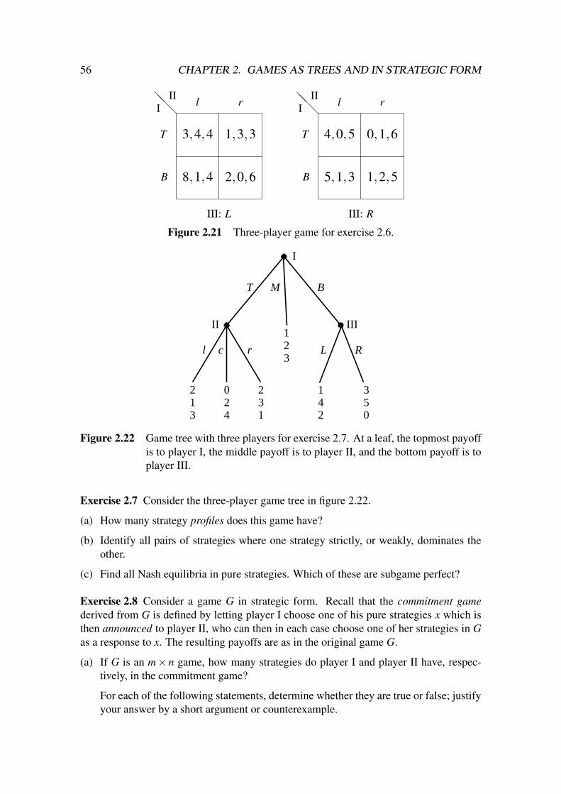
56 CHAPTER 2. GAMES AS TREES AND IN STRATEGIC FORM
@@@I
II
T
B
l r
3,4,4 1,3,3
8,1,4 2,0,6
III: L
@@@I
II
T
B
l r
4,0,5 0,1,6
5,1,3 1,2,5
III: R
Figure 2.21 Three-player game for exercise 2.6.
����
����
����
IIIII
I
M B
L R
123
142
350
l c r
213
024
231
T
Figure 2.22 Game tree with three players for exercise 2.7. At a leaf, the topmost payoffis to player I, the middle payoff is to player II, and the bottom payoff is toplayer III.
Exercise 2.7 Consider the three-player game tree in figure 2.22.
(a) How many strategy profiles does this game have?
(b) Identify all pairs of strategies where one strategy strictly, or weakly, dominates theother.
(c) Find all Nash equilibria in pure strategies. Which of these are subgame perfect?
Exercise 2.8 Consider a game G in strategic form. Recall that the commitment gamederived from G is defined by letting player I choose one of his pure strategies x which isthen announced to player II, who can then in each case choose one of her strategies in Gas a response to x. The resulting payoffs are as in the original game G.
(a) If G is an m× n game, how many strategies do player I and player II have, respec-tively, in the commitment game?
For each of the following statements, determine whether they are true or false; justifyyour answer by a short argument or counterexample.
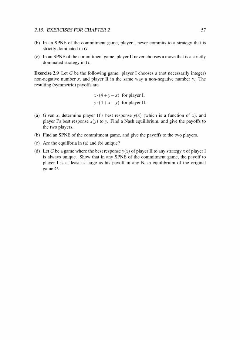
2.15. EXERCISES FOR CHAPTER 2 57
(b) In an SPNE of the commitment game, player I never commits to a strategy that isstrictly dominated in G.
(c) In an SPNE of the commitment game, player II never chooses a move that is a strictlydominated strategy in G.
Exercise 2.9 Let G be the following game: player I chooses a (not necessarily integer)non-negative number x, and player II in the same way a non-negative number y. Theresulting (symmetric) payoffs are
x · (4+ y− x) for player I,
y · (4+ x− y) for player II.
(a) Given x, determine player II’s best response y(x) (which is a function of x), andplayer I’s best response x(y) to y. Find a Nash equilibrium, and give the payoffs tothe two players.
(b) Find an SPNE of the commitment game, and give the payoffs to the two players.
(c) Are the equilibria in (a) and (b) unique?
(d) Let G be a game where the best response y(x) of player II to any strategy x of player Iis always unique. Show that in any SPNE of the commitment game, the payoff toplayer I is at least as large as his payoff in any Nash equilibrium of the originalgame G.

58 CHAPTER 2. GAMES AS TREES AND IN STRATEGIC FORM

Chapter 3
Mixed strategy equilibria
This chapter studies mixed strategy equilibria, extending the considerations of chapter 2.
3.1 Learning objectives
After studying this chapter, you should be able to:
• explain what mixed strategies and mixed equilibria are;
• state the main theorems about mixed strategies: the best response condition, Nash’stheorem on the existence of mixed equilibria, and the minimax theorem;
• find mixed equilibria of small bimatrix games, using geometric tools like the upperenvelope method where necessary;
• give the definition of a degenerate game, and find all equilibria of small degenerategames;
• explain the concept of max-min strategies and their importance for zero-sum games,and apply this to given games.
3.2 Further reading
The strong emphasis on geometric concepts for understanding mixed strategies is notfound to this extent in other books. For zero-sum games, which are the subject of sec-tion 3.14, a detailed treatment is given in the following book:
• Mendelson, Elliot Introducing Game Theory and Its Applications. (Chapman & Hall/ CRC, 2004) [ISBN 1584883006].
Later sections and appendices in that book treat, more briefly, also the non-zero-sumgames studied here.
In section 3.5, an “inspection game” is used to motivate mixed strategies. A book oninspection games is
59

60 CHAPTER 3. MIXED STRATEGY EQUILIBRIA
• Avenhaus, Rudolf, and Morton J. Canty Compliance Quantified. (Cambridge Uni-versity Press, 1996) [ISBN 0521019192].
Nash’s central paper is
• Nash, John F. “Non-cooperative games.” Annals of Mathematics, Vol. 54 (1951), pp.286–295.
This paper is easy to obtain. It should be relatively accessible after a study of this chapter.
3.3 Introduction
A game in strategic form does not always have a Nash equilibrium in which each playerdeterministically chooses one of his strategies. However, players may instead randomlyselect from among these pure strategies with certain probabilities. Randomising one’sown choice in this way is called a mixed strategy. A profile of mixed strategies is called amixed equilibrium if no player can gain on average by unilateral deviation. Nash showedin 1951 that any finite strategic-form game has a mixed equilibrium.
In this chapter, we first discuss how a player’s payoffs represent his preference forrandom outcomes via an expected-utility function. This is illustrated first with a single-player decision problem and then with a game whether to comply or not with a legal re-quirement. The game is known as an inspection game between a player II called inspecteeand an inspector as player I. This game has no equilibrium using pure (that is, determin-istic) strategies. However, active randomisation comes up naturally in this game, becausethe inspector can and will choose to inspect only some of the time. The mixed equilibriumin this game demonstrates many aspects of general mixed equilibria, in particular that aplayer’s randomisation probabilities depend on the payoffs of the other player.
We then turn to general two-player games in strategic form, called bimatrix games.The payoff matrices for the two players are convenient to represent expected payoffsvia multiplication with vectors of probabilities which are the players’ mixed strategies.These mixed strategies, as vectors of probabilities, have a geometric interpretation, whichwe study in detail. Mixing with probabilities is geometrically equivalent to taking convexcombinations.
The best response condition gives a convenient, finite condition when a mixed strat-egy is a best response to the mixed strategy of the other player (or against the mixedstrategies of all other players in a game with more than two players, which we do notconsider). Namely, only the pure strategies that are best responses are allowed to havepositive probability. These pure best responses must have maximal, and hence equal, ex-pected payoff. This is stated as an “obvious fact” in Nash’s paper, and it is not hard toprove. However, the best response condition is central for understanding and computingmixed-strategy equilibria.
In section 3.10, we state and prove Nash’s theorem that every game has an equilib-rium. We follow Nash’s original proof, and state and briefly motivate Brouwer’s fixedpoint theorem used in that proof, but do not prove the fixed point theorem itself.

3.4. EXPECTED-UTILITY PAYOFFS 61
Sections 3.11–3.13 show how to find equilibria in bimatrix games, in particular whenone player has only two strategies.
The special and interesting case of zero-sum games is treated in section 3.14.
3.4 Expected-utility payoffs
The payoffs in a game represent a player’s preferences, in that higher payoffs correspondto more desirable outcomes for the player. In this sense, the payoffs have the role of an“ordinal” utility function, meaning that only the order of preference is important. Forexample, the order among payoffs 0, 8, and 10 can equally be represented by the numbers0, 2, and 10.
As soon as the outcome is random, the payoffs also represent a “cardinal” utility,which means that the relative size of the numbers also matters. The reason is that aver-age (that is, expected) payoffs are considered to represent the preference for the randomoutcomes. For example, the payoffs 0, 8, and 10 do not represent the same preferencesas 0, 2 and 10 when the player has to decide between a coin-toss that gives 0 or 10 withprobability 1/2 each, which is a risky choice, or taking the “middle” payoff. The expectedpayoff of the coin-toss is 5, which is larger than 2 but smaller than 8, so it matters whetherthe middle payoff is 2 or 8. In a game, a player’s payoffs always represent his “expectedutility” function in the sense that the payoffs can be weighted with probabilities in orderto represent the player’s preference for a random outcome.
0
10
0.9 0.1
90
comply cheat
Figure 3.1 One-player decision problem to decide between “comply” and “cheat”. Thisproblem demonstrates expected-utility payoffs. With these payoffs, theplayer is indifferent.
As a concrete example, figure 3.1 shows a game with a single player who can decideto comply with a regulation, like to buy a parking permit, or to cheat otherwise. Thepayoff when she chooses to comply is 0. Cheating involves a 10 percent chance of gettingcaught and having to pay a penalty, stated as the negative payoff −90, and otherwise a 90percent chance of gaining a payoff of 10. With these numbers, cheating leads to a randomoutcome with an expected payoff of 0.9× 10 + 0.1× (−90), which is zero, so that theplayer is exactly indifferent (prefers neither one nor the other) between her two availablemoves.

62 CHAPTER 3. MIXED STRATEGY EQUILIBRIA
If the payoffs are monetary amounts, each payoff unit standing for a dollar, say, onewould not necessarily assume such a risk neutrality on the part of the player. In practice,decision-makers are typically risk averse, meaning they prefer the safe payoff of 0 to thegamble with an expectation of 0.
In a game-theoretic model with random outcomes, as in the game above, the payoffis not necessarily to be interpreted as money. Rather, the player’s attitude towards riskis incorporated into the payoff figure as well. To take our example, the player faces apunishment or reward when cheating, depending on whether she is caught or not. Supposethat the player’s decision only depends on the probability of being caught, which is 0.1 infigure 3.1, so that she would cheat if that probability was zero. Moreover, set the rewardfor cheating arbitrarily to 10 units, as in the figure above, and suppose that being caughthas clearly defined consequences for the player, like regret and losing money and time.Then there must be a certain probability of getting caught where the player in the abovegame is indifferent, say 4 percent. This determines the utility−u, say, for “getting caught”by the equation
0 = 0.96×10+0.04× (−u)
which states equal expected utility for the choices “comply” and “cheat”. This equationis equivalent to u = 9.6/0.04 = 240. That is, in the above game, the negative utility−90 would have to be replaced by −240 to reflect the player’s attitude towards the riskof getting caught. With that payoff, she will now prefer to comply if the probability ofgetting caught stays at 0.1.
The point of this consideration is to show that payoffs exist, and can be constructed,that represent a player’s preference for a risky outcome, as measured by the resultingexpected payoff. These payoffs do not have to represent money. The existence of suchexpected-utility payoffs depends on a certain consistency of the player when facing choiceswith random outcomes. This can be formalised, but the respective theory, known as thevon Neumann–Morgenstern axioms for expected utility, is omitted here for brevity.
In practice, the risk attitude of a player may not be known. A game-theoretic analysisshould be carried out for different choices of the payoff parameters in order to test howmuch they influence the results. Often, these parameters represent the “political” featuresof a game-theoretic model, those most sensitive to subjective judgement, compared tothe more “technical” part of a solution. In particular, there are more involved variantsof the inspection game discussed in the next section. In those more complicated models,the technical part often concerns the optimal usage of limited inspection resources, likemaximising the probability of catching a player who wants to cheat. A separate step after-wards is the “political decision” when to declare that the inspectee has actually cheated.Such models and practical issues are discussed in the book by Avenhaus and Canty, Com-pliance Quantified (see section 3.2).
3.5 Example: Compliance inspections
Suppose a player, whom we simply call “inspectee”, must fulfil some legal obligation(such as buying a transport ticket, or paying tax). The inspectee has an incentive to violate
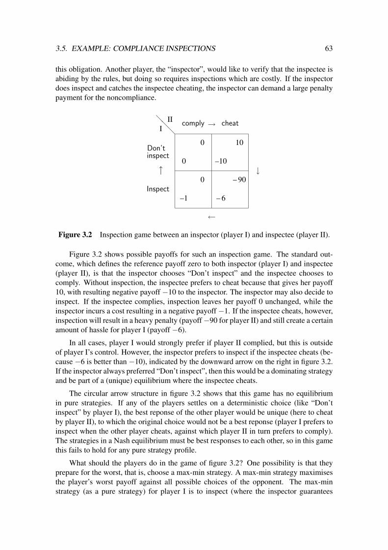
3.5. EXAMPLE: COMPLIANCE INSPECTIONS 63
this obligation. Another player, the “inspector”, would like to verify that the inspectee isabiding by the rules, but doing so requires inspections which are costly. If the inspectordoes inspect and catches the inspectee cheating, the inspector can demand a large penaltypayment for the noncompliance.
@@
@
0
0
–1
0
–10
10
– 6
– 90
III
Don’tinspect
Inspect
comply cheat
↑ ↓
→
←
Figure 3.2 Inspection game between an inspector (player I) and inspectee (player II).
Figure 3.2 shows possible payoffs for such an inspection game. The standard out-come, which defines the reference payoff zero to both inspector (player I) and inspectee(player II), is that the inspector chooses “Don’t inspect” and the inspectee chooses tocomply. Without inspection, the inspectee prefers to cheat because that gives her payoff10, with resulting negative payoff −10 to the inspector. The inspector may also decide toinspect. If the inspectee complies, inspection leaves her payoff 0 unchanged, while theinspector incurs a cost resulting in a negative payoff−1. If the inspectee cheats, however,inspection will result in a heavy penalty (payoff−90 for player II) and still create a certainamount of hassle for player I (payoff −6).
In all cases, player I would strongly prefer if player II complied, but this is outsideof player I’s control. However, the inspector prefers to inspect if the inspectee cheats (be-cause −6 is better than −10), indicated by the downward arrow on the right in figure 3.2.If the inspector always preferred “Don’t inspect”, then this would be a dominating strategyand be part of a (unique) equilibrium where the inspectee cheats.
The circular arrow structure in figure 3.2 shows that this game has no equilibriumin pure strategies. If any of the players settles on a deterministic choice (like “Don’tinspect” by player I), the best reponse of the other player would be unique (here to cheatby player II), to which the original choice would not be a best reponse (player I prefers toinspect when the other player cheats, against which player II in turn prefers to comply).The strategies in a Nash equilibrium must be best responses to each other, so in this gamethis fails to hold for any pure strategy profile.
What should the players do in the game of figure 3.2? One possibility is that theyprepare for the worst, that is, choose a max-min strategy. A max-min strategy maximisesthe player’s worst payoff against all possible choices of the opponent. The max-minstrategy (as a pure strategy) for player I is to inspect (where the inspector guarantees

64 CHAPTER 3. MIXED STRATEGY EQUILIBRIA
himself payoff −6), and for player II it is to comply (which guarantees her payoff 0).However, this is not a Nash equilibrium and hence not a stable recommendation to thetwo players, because player I could switch his strategy and improve his payoff.
A mixed strategy of player I in this game is to inspect only with a certain probability.In the context of inspections, randomising is also a practical approach that reduces costs.Even if an inspection is not certain, a sufficiently high chance of being caught shoulddeter from cheating, at least to some extent.
The following considerations show how to find the probability of inspection that willlead to an equilibrium. If the probability of inspection is very low, for example onepercent, then player II receives (irrespective of that probability) payoff 0 for complying,and payoff 0.99×10+0.01× (−90) = 9, which is bigger than zero, for cheating. Hence,player II will still cheat, just as in the absence of inspection.
If the probability of inspection is much higher, for example 0.2, then the expectedpayoff for “cheat” is 0.8× 10 + 0.2× (−90) = −10, which is less than zero, so thatplayer II prefers to comply. If the inspection probability is either too low or too high, thenplayer II has a unique best response. As shown above, such a pure strategy cannot be partof an equilibrium.
Hence, the only case where player II herself could possibly randomise between herstrategies is if both strategies give her the same payoff, that is, if she is indifferent. Asstated and proved formally in theorem 3.1 below, it is never optimal for a player to assigna positive probability to a pure strategy that is inferior to other pure strategies, given whatthe other players are doing. It is not hard to see that player II is indifferent if and onlyif player I inspects with probability 0.1, because then the expected payoff for cheating is0.9×10+0.1× (−90) = 0, which is then the same as the payoff for complying.
With this mixed strategy of player I (don’t inspect with probability 0.9 and inspectwith probability 0.1), player II is indifferent between her strategies. Hence, she can mixthem (that is, play them randomly) without losing payoff. The only case where, in turn,the original mixed strategy of player I is a best response is if player I is indifferent. Ac-cording to the payoffs in figure 3.2, this requires player II to comply with probability 0.8and to cheat with probability 0.2. The expected payoffs to player I are then for “Don’tinspect” 0.8×0+0.2×(−10) =−2, and for “Inspect” 0.8×(−1)+0.2×(−6) =−2, sothat player I is indeed indifferent, and his mixed strategy is a best response to the mixedstrategy of player II.
This defines the only Nash equilibrium of the game. It uses mixed strategies and istherefore called a mixed equilibrium. The resulting expected payoffs are −2 for player Iand 0 for player II.
The preceding analysis shows that the game in figure 3.2 has a mixed equilibrium,where the players choose their pure strategies according to certain probabilities. Theseprobabilities have several noteworthy features.
First, the equilibrium probability of 0.1 for inspecting makes player II indifferentbetween complying and cheating. As explained in section 3.4 above, this requires payoffsto be expected utilities.
3.6. BIMATRIX GAMES 65
Secondly, mixing seems paradoxical when the player is indifferent in equilibrium. Ifplayer II, for example, can equally well comply or cheat, why should she gamble? Inparticular, she could comply and get payoff zero for certain, which is simpler and safer.The answer is that precisely because there is no incentive to choose one strategy overthe other, a player can mix, and only in that case there can be an equilibrium. If player IIwould comply for certain, then the only optimal choice of player I is not to inspect, makingthe choice of complying not optimal, so this is not an equilibrium.
The least intuitive aspect of mixed equilibrium is that the probabilities depend onthe opponent’s payoffs and not on the player’s own payoffs (as long as the qualitativepreference structure, represented by the arrows, remains intact). For example, one wouldexpect that raising the penalty −90 in figure 3.2 for being caught lowers the probabilityof cheating in equilibrium. In fact, it does not. What does change is the probability ofinspection, which is reduced until the inspectee is indifferent.
3.6 Bimatrix games
In the following, we discuss mixed equilibria for general games in strategic form. Wealways assume that each player has only a finite number of given pure strategies. In orderto simplify notation, we consider the case of two players. Many definitions and resultscarry over without difficulty to the case of more than two players.
Recall that a game in strategic form is specified by a finite set of “pure” strategiesfor each player, and a payoff for each player for each strategy profile, which is a tupleof strategies, one for each player. The game is played by each player independentlyand simultaneously choosing one strategy, whereupon the players receive their respectivepayoffs.
For two players, a game in strategic form is also called a bimatrix game (A,B). Here,A and B are two payoff matrices. By definition, they have equal dimensions, that is, theyare both m×n matrices, having m rows and n columns. The m rows are the pure strategiesi of player I and the n columns are the pure strategies j of player II. For a row i, where1≤ i≤m, and column j, where 1≤ j≤ n, the matrix entry of A is ai j as payoff to player I,and the matrix entry of B is bi j as payoff to player II.
Usually, we depict such a game as a table with m rows and n columns, so that eachcell of the table corresponds to a pure strategy pair (i, j), and we enter both payoffs ai jand bi j in that cell, ai j in the lower-left corner, preferably written in red if we have coloursat hand, and bi j in the upper-right corner of the cell, displayed in blue. The “red” numbersare then the entries of the matrix A, the “blue” numbers those of the matrix B. It does notmatter if we take two matrices A and B, or a single table where each cell has two entries(the respective components of A and B).
A mixed strategy is a randomised strategy of a player. It is defined as a probabilitydistribution on the set of pure strategies of that player. This is played as an “active ran-domisation”: Using a lottery device with the given probabilities, the player picks eachpure strategy according to its probability. When a player plays according to a mixed

66 CHAPTER 3. MIXED STRATEGY EQUILIBRIA
strategy, the other player is not supposed to know the outcome of the lottery. Rather, it isassumed that the opponent knows that the strategy chosen by the player is a random event,and bases his or her decision on the resulting distribution of payoffs. The payoffs are then“weighted with their probabilities” to determine the expected payoff , which represents theplayer’s preference, as explained in section 3.4.
A pure strategy is a special mixed strategy. Namely, consider a pure strategy i ofplayer I. Then the mixed strategy x that selects i with probability one and any other purestrategy with probability zero is effectively the same as the pure strategy i, because xchooses i with certainty. The resulting expected payoff is the same as the pure strategypayoff, because any unplayed strategy has probability zero and hence does not affect theexpected payoff, and the pure strategy i is weighted with probability one.
3.7 Matrix notation for expected payoffs
Unless specified otherwise, we assume that in the two-player game under consideration,player I has m strategies and player II has n strategies. The pure strategies of player I,which are the m rows of the bimatrix game, are denoted by i = 1, . . . ,m, and the purestrategies of player II, which are the n columns of the bimatrix game, are denoted byj = 1, . . . ,n.
A mixed strategy is determined by the probabilities that it assigns to the player’s purestrategies. For player I, a mixed strategy x can therefore be identified with the m-tupleof probabilities (x1,x2, . . . ,xm) that it assigns to the pure strategies 1,2, . . . ,m of player I.We can therefore consider x as an element of m-space (written Rm). We assume that thevector x with m components is a row vector, that is, a 1×m matrix with a single row andm columns. This will allow us to write expected payoffs in a short way.
A mixed strategy y of player II is an n-tuple of probabilities y j for playing the purestrategies j = 1, . . . ,n. That is, y is an element of Rn. We write y as a column vector,as (y1,y2, . . . ,yn)>, that is, the row vector (y1,y2, . . . ,yn) transposed. Transposition ingeneral applies to any matrix. The transpose B> of the payoff matrix B, for example,is the n×m matrix where the entry in row j and column i is bi j, because transpositionmeans exchanging rows and columns. A column vector with n components is thereforeconsidered as an n×1 matrix; transposition gives a row vector, a 1×n matrix.
Normally, all vectors are considered as column vectors, so Rn is equal to Rn×1, theset of all n× 1 matrices with n rows and one column. We have made an exception indefining a mixed strategy x of player I as a row vector. Whether we mean row or columnvectors will be clear from the context.
Suppose that player I uses the mixed strategy x and that player II uses the mixedstrategy y. With these conventions, we can now succinctly express the expected payoff toplayer I as xAy, and the expected payoff to player II as xBy.
In order to see this, recall that the matrix product CD of two matrices C and D isdefined when the number of columns of C is equal to the number of rows of D. That is,C is a p×q matrix, and D is a q× r matrix. The product CD is then a p× r matrix with
3.7. MATRIX NOTATION FOR EXPECTED PAYOFFS 67
entry ∑qk=1 cikdk j in row i and column j, where cik and dk j are the respective entries of C
and D. Matrix multiplication is associative, that is, for another r× s matrix E the matrixproduct CDE is a p× s matrix, which can be computed either as (CD)E or as C(DE).
For mixed strategies x and y, we read xAy and xBy as matrix products. This worksbecause x, considered as a matrix, is of dimension 1×m, both A and B are of dimensionm× n, and y is of dimension n× 1. The result is a 1× 1 matrix, that is, a single realnumber.
It is best to think of xAy being computed as x(Ay), that is, as the product of a rowvector x that has m components with a column vector Ay that has m components. (Thematrix product of two such vectors is also known as the scalar product of these twovectors.) The column vector Ay has m rows. We denote the entry of Ay in row i by (Ay)ifor each row i. It is given by
(Ay)i =n
∑j=1
ai j y j for 1≤ i≤ m. (3.1)
That is, the entries ai j of row i of player I’s payoff matrix A are multiplied with theprobabilities y j of their columns, so (Ay)i is the expected payoff to player I when playingrow i. One can also think of y j as a linear coefficient of the jth column of the matrix A.That is, Ay is the linear combination of the column vectors of A, each multiplied with itsprobability under y. This linear combination Ay is a vector of expected payoffs, with oneexpected payoff (Ay)i for each row i.
Furthermore, xAy is the expected payoff to player I when the players use x and y,because
x(Ay) =m
∑i=1
xi(Ay)i =m
∑i=1
xi
n
∑j=1
ai j y j =m
∑i=1
n
∑j=1
(xi y j)ai j . (3.2)
Because the players choose their pure strategies i and j independently, the probability thatthey choose the pure strategy pair (i, j) is the product xi y j of these probabilities, which isthe coefficient of the payoff ai j in (3.2).
Analogously, xBy is the expected payoff to player II when the players use the mixedstrategies x and y. Here, it is best to read this as (xB)y. The vector xB, as the productof a 1×m with an m×n matrix, is a 1×n matrix, that is, a row vector. Each column ofthat row corresponds to a strategy j of player II, for 1≤ j ≤ n. We denote the respectivecolumn entry by (xB) j. It is given by ∑m
i=1 xi bi j, which is the scalar product of x with thejth column of B. That is, (xB) j is the expected payoff to player II when player I plays xand player II plays the pure strategy j. If these numbers are multiplied with the columnprobabilities y j and added up, then the result is the expected payoff to player II, which inanalogy to (3.2) is given by
(xB)y =n
∑j=1
(xB) j y j =n
∑j=1
(m
∑i=1
xi bi j
)y j =
n
∑j=1
m
∑i=1
(xi y j)bi j . (3.3)

68 CHAPTER 3. MIXED STRATEGY EQUILIBRIA
3.8 Convex combinations and mixed strategy sets
It is useful to regard mixed strategy vectors as geometric objects. A mixed strategy x ofplayer I assigns probabilities xi to the pure strategies i. The pure strategies, in turn, arespecial mixed strategies, namely the unit vectors in Rm, for example (1,0,0), (0,1,0),(0,0,1) if m = 3. The mixed strategy (x1,x2,x3) is then a linear combination of the purestrategies, namely x1 ·(1,0,0)+x2 ·(0,1,0)+x3 ·(0,0,1), where the linear coefficients arejust the probabilities. Such a linear combination is called a convex combination becausethe coefficients sum to one and are non-negative.
{x+ p(y− x) | p ∈ R}0
yb
ax
c
Figure 3.3 The line through the points x and y is given by the points x+ p(y−x) wherep ∈ R. Examples are point a for p = 0.6, point b for p = 1.5, and pointc when p = −0.4. The line segment connecting x and y results when p isrestricted to 0≤ p≤ 1.
Figure 3.3 shows two points x and y, here in the plane, but the picture may also beregarded as a suitable view of the situation in a higher-dimensional space. The line thatgoes through the points x and y is obtained by adding to the point x, regarded as a vector,any multiple of the difference y− x. The resulting vector x + p · (y− x), for p ∈ R, givesx when p = 0, and y when p = 1. Figure 3.3 gives some examples a, b, c of other points.When 0≤ p≤ 1, as for point a, the resulting points give the line segment joining x and y.If p > 1, then one obtains points on the line through x and y on the other side of y relativeto x, like the point b in figure 3.3. For p < 0, the corresponding point, like c in figure 3.3,is on that line but on the other side of x relative to y.
The expression x+ p(y−x) can be re-written as (1− p)x+ py, where the given pointsx and y appear only once. This expression (with 1− p as the coefficient of the first vectorand p of the second) shows how the line segment joining x to y corresponds to the realinterval [0,1] for the possible values of p, with the endpoints 0 and 1 of the intervalcorresponding to the endpoints x and y, respectively, of the line segment.
In general, a convex combination of points z1,z2, . . . ,zk in some space is given as anylinear combination p1 · z1 + p2 · z2 + · · ·+ pk · zk where the linear coefficients p1, . . . , pkare non-negative and sum to one. The previously discussed case corresponds to z1 = x,z2 = y, p1 = 1− p, and p2 = p ∈ [0,1].
A set of points is called convex if it contains with any points z1,z2, . . . ,zk also everyconvex combination of these points. Equivalently, one can show that a set is convex if it
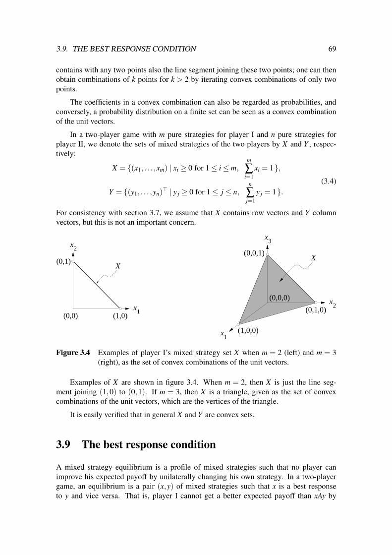
3.9. THE BEST RESPONSE CONDITION 69
contains with any two points also the line segment joining these two points; one can thenobtain combinations of k points for k > 2 by iterating convex combinations of only twopoints.
The coefficients in a convex combination can also be regarded as probabilities, andconversely, a probability distribution on a finite set can be seen as a convex combinationof the unit vectors.
In a two-player game with m pure strategies for player I and n pure strategies forplayer II, we denote the sets of mixed strategies of the two players by X and Y , respec-tively:
X = {(x1, . . . ,xm) | xi ≥ 0 for 1≤ i≤ m,m
∑i=1
xi = 1},
Y = {(y1, . . . ,yn)> | y j ≥ 0 for 1≤ j ≤ n,n
∑j=1
y j = 1}.(3.4)
For consistency with section 3.7, we assume that X contains row vectors and Y columnvectors, but this is not an important concern.
x1
x2
(0,0) (1,0)
(0,1)X
x2
x3
x1
(0,0,1)
(0,1,0)
(1,0,0)
X
(0,0,0)
Figure 3.4 Examples of player I’s mixed strategy set X when m = 2 (left) and m = 3(right), as the set of convex combinations of the unit vectors.
Examples of X are shown in figure 3.4. When m = 2, then X is just the line seg-ment joining (1,0) to (0,1). If m = 3, then X is a triangle, given as the set of convexcombinations of the unit vectors, which are the vertices of the triangle.
It is easily verified that in general X and Y are convex sets.
3.9 The best response condition
A mixed strategy equilibrium is a profile of mixed strategies such that no player canimprove his expected payoff by unilaterally changing his own strategy. In a two-playergame, an equilibrium is a pair (x,y) of mixed strategies such that x is a best responseto y and vice versa. That is, player I cannot get a better expected payoff than xAy by
70 CHAPTER 3. MIXED STRATEGY EQUILIBRIA
choosing any other strategy than x, and player II cannot improve her expected payoff xByby changing y.
It does not seem easy to decide if x is a best response to y among all possible mixedstrategies, that is, if x maximises xAy for all x in X , because X is an infinite set. However,the following theorem, known as the best response condition, shows how to recognise this.This theorem is not difficult but it is important to understand. We discuss it afterwards.
Theorem 3.1 (Best response condition) Let x and y be mixed strategies of player I and II,respectively. Then x is a best response to y if and only if for all pure strategies i of player I,
xi > 0 =⇒ (Ay)i = max{(Ay)k | 1≤ k ≤ m}. (3.5)
Proof. Recall that (Ay)i is the ith component of Ay, which is the expected payoff toplayer I when playing row i, according to (3.1). Let u = max{(Ay)k | 1≤ k ≤ m}, whichis the maximum of these expected payoffs for the pure strategies of player I. Then
xAy =m
∑i=1
xi (Ay)i =m
∑i=1
xi (u− (u− (Ay)i) =m
∑i=1
xi u−m
∑i=1
xi (u− (Ay)i)
= u−m
∑i=1
xi (u− (Ay)i).(3.6)
Because, for any pure strategy i, both xi and the difference of the maximum payoff u andthe payoff (Ay)i for row i is non-negative, the sum ∑m
i=1 xi(u− (Ay)i) is also non-negative,so that xAy≤ u. The expected payoff xAy achieves the maximum u if and only if that sumis zero, that is, if xi > 0 implies (Ay)i = u, as claimed.
Consider the phrase “x is a best response to y” in the preceding theorem. This meansthat among all mixed strategies in X of player I, x gives maximum expected payoff toplayer I. However, the pure best responses to y in (3.5) only deal with the pure strategiesof player I. Each such pure strategy corresponds to a row i of the payoff matrix. In thatrow, the payoffs ai j are multiplied with the column probabilities y j, and the sum over allcolumns gives the expected payoff (Ay)i for the pure strategy i according to (3.1). Thispure strategy is a best response if and only if no other row gives a higher payoff.
The first point of the theorem is that the condition whether a pure strategy is a bestresponse is very easy to check, as one only has to compute the m expected payoffs (Ay)ifor i = 1, . . . ,m. For example, if player I has three pure strategies (m = 3), and the expectedpayoffs in (3.1) are (Ay)1 = 4, (Ay)2 = 4, and (Ay)3 = 3, then only the first two strategiesare pure best responses. If these expected payoffs are 3, 5, and 3, then only the secondstrategy is a best response. Clearly, at least one pure best response exists, because thenumbers (Ay)k in (3.5) have their maximum u for at least one k. The theorem states thatonly pure best responses i may have positive probability xi if x is to be a best responseto y.
A second consequence of theorem 3.1, used also in its proof, is that a mixed strat-egy can never give a higher payoff than the best pure strategy. This is intuitive because“mixing” amounts to averaging, which is an average weighted with the probabilities, in

3.10. EXISTENCE OF MIXED EQUILIBRIA 71
the way that the overall expected payoff xAy in (3.6) is obtained from those in (3.1) bymultiplying (weighting) each row i with weight xi and summing over all rows i, as shownin (3.2). Consequently, any pure best response i to y is also a mixed best response, so themaximum of xAy for x ∈ X is the same as when x is restricted to the unit vectors in Rm
that represent the pure strategies of player I.
⇒ Try now exercise 3.1 on page 91, with the help of theorem 3.1. This will help youappreciate methods for finding mixed equilibria that you will learn in later sections.You can also answer exercise 3.2 on page 91, which concerns a game with threeplayers.
3.10 Existence of mixed equilibria
In this section, we give the original proof of John Nash from 1951 that shows that anygame with a finite number of players, and finitely many strategies per player, has a mixedequilibrium. This proof uses the following theorem about continuous functions. Thetheorem concerns compact sets; here, a set is compact if it is closed (containing all pointsnear the set) and bounded.
Theorem 3.2 (Brouwer’s fixed point theorem) Let S be a subset of RN that is convexand compact, and let f be a continuous function from S to S. Then f has at least one fixedpoint, that is, a point s in S so that f (s) = s.
We do not prove theorem 3.2, but instead demonstrate its assumptions with exampleswhere not all assumptions hold and the conclusion fails. Consider the function f :R→ Rdefined by f (x) = x + 1. This is clearly a continuous function, and the set R of all realnumbers is closed and convex, but f has no fixed point. Some assumption of the fixedpoint theorem must be violated, and in this case it is compactness, because the set R is notbounded. Consider another function f : [0,1]→ [0,1], given by f (x) = x2. The fixed pointsof this function are 0 and 1. If we consider the function f (x) = x2 as a function on theopen interval (0,1) (which is [0,1] without its endpoints), then this function has no longerany fixed points. In this case, the missing condition is that the function is not defined on aclosed set, which is therefore not compact. Another function is f (x) = 1−x for x∈ {0,1},where the domain of this function has just two elements, so this is a compact set. Thisfunction has no fixed points which is possible because its domain is not convex. Finally,the function on [0,1] defined by f (x) = 1 for 0≤ x≤ 1/2 and by f (x) = 0 for 1/2 < x≤ 1has no fixed point, which is possible in this case because the function is not continuous.These simple examples demonstrate why the assumptions of theorem 3.2 are necessary.
Theorem 3.3 (Nash [1951]) Every finite game has at least one equilibrium in mixedstrategies.
Proof. We will give the proof for two players, to simplify notation. It extends in the samemanner to any finite number of players. The set S that is used in the present context is theproduct of the sets of mixed strategies of the players. Let X and Y be the sets of mixedstrategies of player I and player II as in (3.4), and let S = X ×Y .

72 CHAPTER 3. MIXED STRATEGY EQUILIBRIA
Then the function f :S → S that we are going to construct maps a pair of mixedstrategies (x,y) to another pair f (x,y) = (x,y). Intuitively, a mixed strategy probabilityxi (of player I, similarly y j of player II) is changed to xi, such that it will decrease ifthe pure strategy i does worse than the average of all pure strategies. In equilibrium,all pure strategies of a player that have positive probability do equally well, so no sub-optimal pure strategy can have a probability that is reduced further. This means that themixed strategies do not change, so this is indeed equivalent to the fixed point property(x,y) = (x,y) = f (x,y).
In order to define f as described, consider the following functions χ :X ×Y → Rm
and ψ:X ×Y → Rn (we do not worry whether these vectors are row or column vectors;it suffices that Rm contains m-tuples of real numbers, and similarly Rn contains n-tuples).For each pure strategy i of player I, let χi(x,y) be the ith component of χ(x,y), and for eachpure strategy j of player II, let ψ j(x,y) be the jth component of ψ(x,y). The functions χand ψ are defined by
χi(x,y) = max{0,(Ay)i− xAy}, ψ j(x,y) = max{0,(xB) j− xBy},
for 1≤ i≤ m and 1≤ j ≤ n. Recall that (Ay)i is the expected payoff to player I against ywhen he uses the pure strategy i, and that (xB) j is the expected payoff to player II againstx when she uses the pure strategy j. Moreover, xAy and xBy are the overall expectedpayoffs to player I and player II, respectively. So the difference (Ay)i− xAy is positiveif the pure strategy i gives more than the average xAy against y, zero if it gives the samepayoff, and negative if it gives less. The term χi(x,y) is this difference, except that it isreplaced by zero if the difference is negative. The term ψ j(x,y) is defined analogously.Thus, χ(x,y) is a non-negative vector in Rm, and ψ(x,y) is a non-negative vector in Rn.The functions χ and ψ are continuous.
The pair of vectors (x,y) is now changed by replacing x by x+ χ(x,y) in order to getx, and y by y+ψ(x,y) to get y. Both sums are non-negative. The only problem is that ingeneral these new vectors are no longer probabilities because their components do not sumto one. For that purpose, they are “re-normalised” by the following functions r :Rm→Rm
and s : Rn→ Rn, defined by their components ri and s j, that is, r(x) = (r1(x), . . . ,rm(x)),and s(y) = (s1(y), . . . ,sn(y)):
ri(x1, . . . ,xm) =xi
∑mk=1 xk
, s j(y1, . . . ,yn) =y j
∑nk=1 yk
.
Clearly, if xi ≥ 0 for 1 ≤ i ≤ m and ∑mk=1 xk > 0, then r(x) is defined and is a probability
distribution, that is, an element of the mixed strategy set X . Analogously, s(y) ∈ Y .
The function f :X → Y is now defined by
f (x,y) =(r(x+ χ(x,y)), s(y+ψ(x,y))
).
What is a fixed point (x,y) of that function, so that f (x,y) = (x,y)? Among all strategiesi where xi > 0, consider the smallest pure strategy payoff (Ay)i against y, that is, (Ay)i =min{(Ay)k | xk > 0}. Then (Ay)i ≤ xAy, which is proved analogously to (3.6), so thecomponent χi(x,y) of χ(x,y) is zero. This means that the respective term xi + χi(x,y)

3.11. FINDING MIXED EQUILIBRIA 73
is equal to xi. Conversely, consider any other pure strategy l of player I that gets themaximum payoff (Ay)l = maxk(Ay)k. If that payoff is better than the average xAy, thenclearly χl(x,y) > 0, so that xl + χl(x,y) > xl . Because χk(x,y) ≥ 0 for all k, this implies∑m
k=1(xk + χk(x,y)) > 1, which is the denominator in the re-normalisation with r in r(x+χ(x,y)). This re-normalisation will now decrease the value of xi for the pure strategy iwith (Ay)i ≤ xAy, so the relative weight xi of the pure strategy i decreases. (It would stayunchanged, that is, not decrease, if xi = 0.) But (Ay)l > xAy can only occur if there issome sub-optimal strategy i (with (Ay)i ≤ xAy < (Ay)l) that has positive probability xi. Inthat case, r(x+ χ(x,y)) is not equal to x, so that f (x,y) 6= (x,y).
Analogously, if ψ(x,y) has some component that is positive, then the respective purestrategy of player II has a better payoff than xBy, so y 6= s(y + ψ(x,y)) and (x,y) is not afixed point of f . In that case, y is also not a best response to x.
Hence, the function f has a fixed point (x,y) if and only if both χ(x,y) and ψ(x,y)are zero in all components. But that means that xAy is the maximum possible payoffmaxi(Ay)i against y, and xBy is the maximum possible payoff max j(xB) j against x, thatis, x and y are mutual best responses. The fixed points (x,y) are therefore exactly the Nashequilibria of the game.
3.11 Finding mixed equilibria
How can we find all Nash equilibria of a two-player game in strategic form? It is easy todetermine the Nash equilibria where both players use a pure strategy, because these arethe cells of the payoff table where both payoffs are best-response payoffs, shown by a boxaround that payoff. We now describe how to find mixed strategy equilibria, using the bestresponse condition theorem 3.1.
We first consider 2× 2 games. Our first example above, the inspection game in fig-ure 3.2, has no pure-strategy equilibrium. There we have determined the mixed strategyprobabilities of a player so as to make the other player indifferent between his or herpure strategies, because only then that player will mix between these strategies. This isa consequence of theorem 3.1: Only pure strategies that get maximum, and hence equal,expected payoff can be played with positive probability in equilibrium.
A mixed strategy equilibrium can exist also in 2× 2 games that have pure-strategyequilibria. As an example, consider the battle of sexes game, shown on the left in fig-ure 3.5, which has the pure strategy equilibria (C,c) and (S,s). As indicated by the boxes,the best response of the other player depends on the player’s own strategy: If player Iplays C then player II’s best response is c, and the best response to S is s. Suppose nowthat player I plays a mixed strategy, playing C with probability 1− p and S with prob-ability p. Clearly, when p is close to zero so that player I almost certainly chooses C,the best response will still be c, whereas if p is close to one the best response will be s.Consequently, there is some probability so that player II is indifferent. This probability pis found as follows. Given p, which defines the mixed strategy of player I, the expectedpayoff to player II when she plays c is 2(1− p), and when she plays s that expected payoff

74 CHAPTER 3. MIXED STRATEGY EQUILIBRIA
@@@I
II
C
S
c s
1 0
2 0
0 2
0 1
@@@I
II
C
S
B
c s
1 0
2 0
0 2
0 1
−1 3
4 1
Figure 3.5 Battle of sexes game (left) and a 3×2 game (right) which is the same gamewith an extra strategy B for player I.
is simply p. She is indifferent between c and s if and only if these expected payoffs areequal, that is, 2(1− p) = p or 2 = 3p, that is, p = 2/3. This mixed strategy of player I,where he plays C and S with probabilities 1/3 and 2/3, respectively, gives player II forboth her strategies, the two columns, the same expected payoff 2/3. Then player II canmix between c and s, and a similar calculation shows that player I is indifferent betweenhis two strategies if player II uses the mixed strategy (2/3,1/3), which is the vector ofprobabilities for her two strategies c,s. Then and only then player I gets the same expectedpayoff for both rows, which is 2/3. This describes the mixed equilibrium of the game,which we write as ((1/3,2/3),(2/3,1/3)), as a pair (x,y) of mixed strategies x and y,which are probability vectors.
In short, the rule to find a mixed strategy equilibrium in a 2× 2 game is to makethe other player indifferent, because only in that case can the other player mix. Thisindifference means the expected payoffs for the two opponent strategies have to be equal,and the resulting equation determines the player’s own probability.
The mixed strategy probabilities in the battle of sexes game can be seen relativelyquickly by looking at the payoff matrices: For example, player II must give twice asmuch weight to strategy c compared to s, because player I’s strategy C only gets onepayoff unit from c whereas his strategy S gets two payoff units when player II chooses s.Because the strategy pairs (C,s) and (S,c) give payoff zero, the two rows C and S givethe same expected payoff only when c has probability 2/3 and s has probability 1/3.
We now explain a quick method, the “difference trick”, to find the probabilities ina mixed strategy equilibrium of a general 2× 2 game. Consider the game on the leftin figure 3.6. When player II plays T , then l is a best response, and when player IIplays B, then r is a best response. Consequently, there must be a way to mix T and Bso that player II is indifferent between l and r. We consider now the difference ∆ inpayoffs to the other player for both rows: When player I plays T , then the differencebetween the two payoffs to player II is ∆ = 2− 1 = 1, and when player I plays B, thenthat difference, in absolute value, is ∆ = 7− 3 = 4, as shown on the side of the game.(Note that these differences, when considered as differences between the payoffs for l
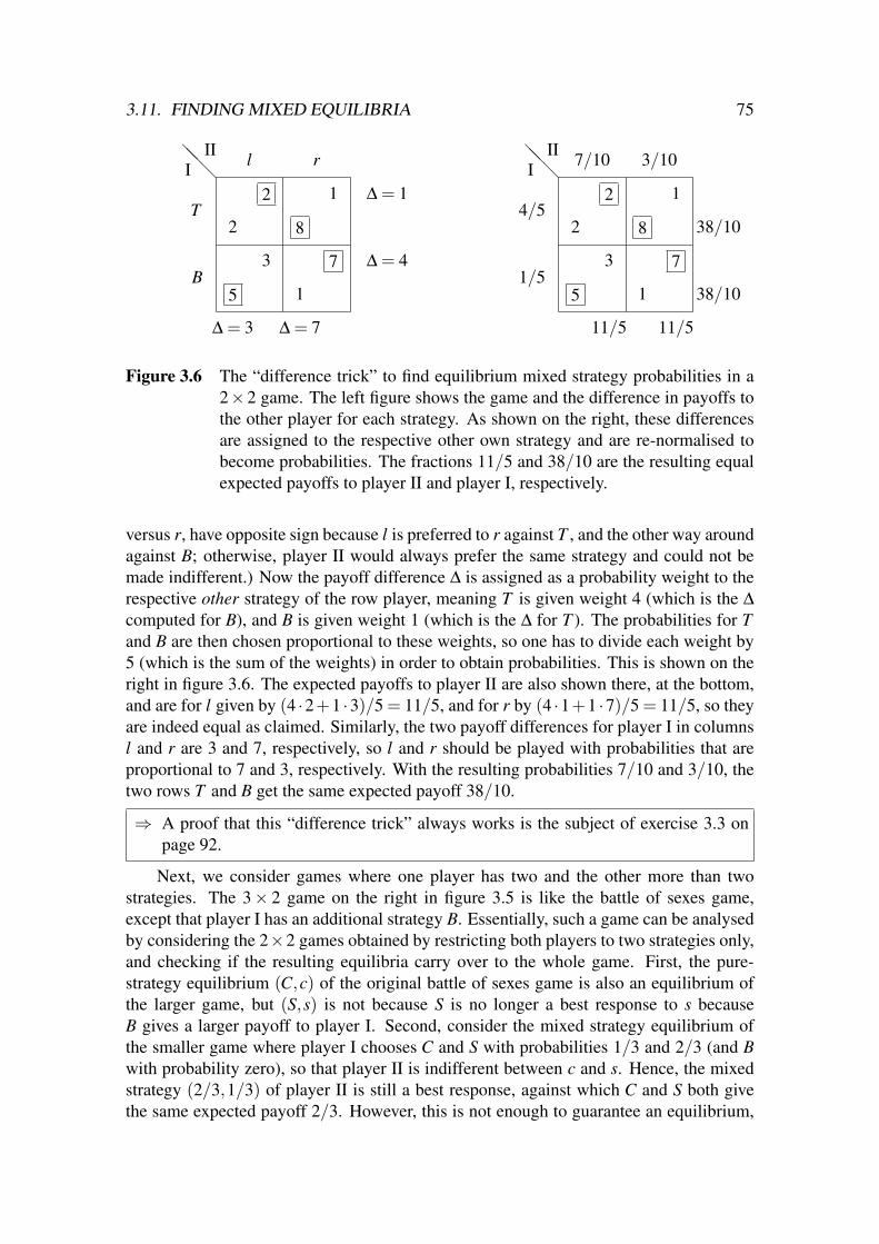
3.11. FINDING MIXED EQUILIBRIA 75
@@@I
II
T
B
l r
2 8
2 1 ∆ = 1
5 1
3 7 ∆ = 4
∆ = 3 ∆ = 7
@@@I
II
4/5
1/5
7/10 3/10
2 8 38/10
2 1
5 1 38/10
3 7
11/5 11/5
Figure 3.6 The “difference trick” to find equilibrium mixed strategy probabilities in a2×2 game. The left figure shows the game and the difference in payoffs tothe other player for each strategy. As shown on the right, these differencesare assigned to the respective other own strategy and are re-normalised tobecome probabilities. The fractions 11/5 and 38/10 are the resulting equalexpected payoffs to player II and player I, respectively.
versus r, have opposite sign because l is preferred to r against T , and the other way aroundagainst B; otherwise, player II would always prefer the same strategy and could not bemade indifferent.) Now the payoff difference ∆ is assigned as a probability weight to therespective other strategy of the row player, meaning T is given weight 4 (which is the ∆computed for B), and B is given weight 1 (which is the ∆ for T ). The probabilities for Tand B are then chosen proportional to these weights, so one has to divide each weight by5 (which is the sum of the weights) in order to obtain probabilities. This is shown on theright in figure 3.6. The expected payoffs to player II are also shown there, at the bottom,and are for l given by (4 ·2+1 ·3)/5 = 11/5, and for r by (4 ·1+1 ·7)/5 = 11/5, so theyare indeed equal as claimed. Similarly, the two payoff differences for player I in columnsl and r are 3 and 7, respectively, so l and r should be played with probabilities that areproportional to 7 and 3, respectively. With the resulting probabilities 7/10 and 3/10, thetwo rows T and B get the same expected payoff 38/10.
⇒ A proof that this “difference trick” always works is the subject of exercise 3.3 onpage 92.
Next, we consider games where one player has two and the other more than twostrategies. The 3× 2 game on the right in figure 3.5 is like the battle of sexes game,except that player I has an additional strategy B. Essentially, such a game can be analysedby considering the 2×2 games obtained by restricting both players to two strategies only,and checking if the resulting equilibria carry over to the whole game. First, the pure-strategy equilibrium (C,c) of the original battle of sexes game is also an equilibrium ofthe larger game, but (S,s) is not because S is no longer a best response to s becauseB gives a larger payoff to player I. Second, consider the mixed strategy equilibrium ofthe smaller game where player I chooses C and S with probabilities 1/3 and 2/3 (and Bwith probability zero), so that player II is indifferent between c and s. Hence, the mixedstrategy (2/3,1/3) of player II is still a best response, against which C and S both givethe same expected payoff 2/3. However, this is not enough to guarantee an equilibrium,
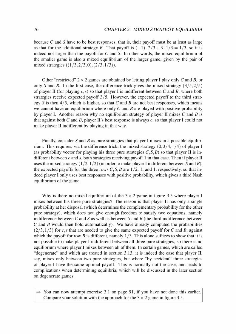
76 CHAPTER 3. MIXED STRATEGY EQUILIBRIA
because C and S have to be best responses, that is, their payoff must be at least as largeas that for the additional strategy B. That payoff is (−1) · 2/3 + 3 · 1/3 = 1/3, so it isindeed not larger than the payoff for C and S. In other words, the mixed equilibrium ofthe smaller game is also a mixed equilibrium of the larger game, given by the pair ofmixed strategies ((1/3,2/3,0),(2/3,1/3)).
Other “restricted” 2×2 games are obtained by letting player I play only C and B, oronly S and B. In the first case, the difference trick gives the mixed strategy (3/5,2/5)of player II (for playing c,s) so that player I is indifferent between C and B, where bothstrategies receive expected payoff 3/5. However, the expected payoff to the third strat-egy S is then 4/5, which is higher, so that C and B are not best responses, which meanswe cannot have an equilibrium where only C and B are played with positive probabilityby player I. Another reason why no equilibrium strategy of player II mixes C and B isthat against both C and B, player II’s best response is always c, so that player I could notmake player II indifferent by playing in that way.
Finally, consider S and B as pure strategies that player I mixes in a possible equilib-rium. This requires, via the difference trick, the mixed strategy (0,3/4,1/4) of player I(as probability vector for playing his three pure strategies C,S,B) so that player II is in-different between c and s, both strategies receiving payoff 1 in that case. Then if player IIuses the mixed strategy (1/2,1/2) (in order to make player I indifferent between S and B),the expected payoffs for the three rows C,S,B are 1/2, 1, and 1, respectively, so that in-deed player I only uses best responses with positive probability, which gives a third Nashequilibrium of the game.
Why is there no mixed equilibrium of the 3× 2 game in figure 3.5 where player Imixes between his three pure strategies? The reason is that player II has only a singleprobability at her disposal (which determines the complementary probability for the otherpure strategy), which does not give enough freedom to satisfy two equations, namelyindifference between C and S as well as between S and B (the third indifference betweenC and B would then hold automatically). We have already computed the probabilities(2/3,1/3) for c,s that are needed to give the same expected payoff for C and B, againstwhich the payoff for row B is different, namely 1/3. This alone suffices to show that it isnot possible to make player I indifferent between all three pure strategies, so there is noequilibrium where player I mixes between all of them. In certain games, which are called“degenerate” and which are treated in section 3.13, it is indeed the case that player II,say, mixes only between two pure strategies, but where “by accident” three strategiesof player I have the same optimal payoff. This is normally not the case, and leads tocomplications when determining equilibria, which will be discussed in the later sectionon degenerate games.
⇒ You can now attempt exercise 3.1 on page 91, if you have not done this earlier.Compare your solution with the approach for the 3×2 game in figure 3.5.

3.12. THE UPPER ENVELOPE METHOD 77
3.12 The upper envelope method
The topic of this section is the “upper-envelope” diagram that simplifies finding mixedequilibria, in particular of games where one player has only two strategies.
The left graph in figure 3.7 shows the upper-envelope diagram for the left game infigure 3.5. This diagram is a plot of the expected payoff of one player against the mixedstrategy of the other player. We use this typically when that mixed strategy is determinedby a single probability, that is, we consider a player who has only two pure strategies,in this example player II. The horizontal axis represents the probability for playing thesecond pure strategy s of player II, so this is q = prob(s). In the vertical direction, we plotthe resulting expected payoffs to the other player, here player I, for his pure strategies. Inthis game, this is the expected payoff 1−q when he plays row C, and the expected payoff2q when he plays row S. The plots are lines because expected payoffs are linear functionsof the mixed strategy probabilities.
These lines are particularly easy to obtain graphically. To see this, consider row Cof player I. When player II plays her left strategy c (where q = 0), row C gives payoff 1(according to the table of payoffs to player I). When player II plays her right strategy s(where q = 1), row C gives payoff 0. The probabilities q = 0 or q = 1 and correspondingpayoffs define the two endpoints with co-ordinates (0,1) and (1,0) of a line that describesthe expected payoff 1− q as a function of q, which consists of the points (q,1− q) forq∈ [0,1]. As explained in section 3.8 above, this line is just the set of convex combinations(1− q) · (0,1) + q · (1,0) of the two endpoints. The first component of such a convexcombination is always q and second component (1− q) · 1 + q · 0 is the expected payoff.For row S, this expected payoff is (1−q) ·0 + q ·2, so the line of expected payoffs for Sconnects the left endpoint (0,0) with the right endpoint (1,2).
0 1
payoff to I
2
1
0 prob(s)
1/3
CS
1
2
1
0 prob(s)
1/3
−1
payoff to I
3
1/2
C S
B
Figure 3.7 Upper envelope of expected payoffs to player I for the two games in fig-ure 3.5.
The upper-envelope diagram can also be described as the “goalpost” method. First,identify a player who has only two pure strategies (here player II). Second, plot the

78 CHAPTER 3. MIXED STRATEGY EQUILIBRIA
probability (here q) for the second of these pure strategies horizontally, along the interval[0,1]. Third, erect a vertical line (a “goalpost”) at the left endpoint 0 and at the rightendpoint 1 of that interval. Fourth, do the following for each pure strategy of the otherplayer (which are here rows C and S for player I): Mark the payoff (as given in the gamedescription) against the left strategy (of player II, that is, against q = 0) as a “height” onthe left goalpost, and against the right strategy (q = 1) as a height on the right goalpost,and connect the two heights by a line, which gives the expected payoff as a function of qfor 0≤ q≤ 1.
Note that for these goalposts it is very useful to consider player II’s mixed strategyas the vector of probabilities (1−q,q) (according to the second step above), because thenthe left goalpost corresponds to the left strategy of player II, and the right goalpost to theright strategy of player II. (This would not be the case if q was taken as the probabilityfor the left strategy, writing player II’s mixed strategy as (q,1− q), because then q = 0would be the left goalpost but represent the right pure strategy of player II, creating anunnecessary source of confusion.)
In the left diagram in figure 3.7, the two lines of expected payoffs for rows C and Sobviously intersect exactly where player I is indifferent between these two rows, whichhappens when q = 1/3. However, the diagram not only gives information about thisindifference, but about player I’s preference in general: Any pure strategy that is a bestresponse of player I is obviously the topmost line segment of all the lines describing theexpected payoffs. Here, row C is a best response whenever 0 ≤ q ≤ 1/3, and row S isa best response whenever 1/3 ≤ q ≤ 1, with indifference between C and S exactly whenq = 1/3. The upper envelope of expected payoffs is the maximum of the lines that describethe expected payoffs for the different pure strategies, and it is indicated by the bold linesegments in the diagram. Marking this upper envelope in bold is therefore the fifth stepof the “goalpost” method.
The upper envelope is of particular use when a player has more than two pure strate-gies, because mixed equilibria of a 2× 2 are anyhow quickly determined with the “dif-ference trick”. Consider the upper-envelope diagram on the right of figure 3.7, for the3×2 game in figure 3.5. The extra strategy B of player I gives the line connecting height−1 on the left goalpost to height 3 on the right goalpost, which shows that B is a bestresponse for all q so that 1/2≤ q≤ 1, with indifference between S and B when q = 1/2.The upper envelope consists of three line segments for the three pure strategies C, S, andB of player I. Moreover, there are only two points where player I is indifferent betweenany two such strategies, namely between C and S when q = 1/3, and between S and Bwhen q = 1/2. These two points, indicated by small circles on the upper envelope, givethe only two mixed strategy probabilities of player II where player I can mix between twopure strategies (the small circle for q = 0 corresponds to the pure equilibrium strategy c).There is a third indifference between C and B, for q = 2/5, where the two lines for C andB intersect, but this intersection point is below the line for S and hence not on the upperenvelope. Consequently, it does not have to be investigated as a possible mixed strategyequilibrium strategy where player I mixes between the two rows C and B because they arenot best responses.

3.12. THE UPPER ENVELOPE METHOD 79
Given these candidates of mixtures for player I, we can quickly find if and how thetwo respective pure strategies can be mixed in order to make player II indifferent usingthe difference trick, as described in the previous section.
So the upper envelope restricts the pairs of strategies that need to be tested as possiblestrategies that are mixed in equilibrium. Exercise 3.4, for example, gives a 2× 5 game,where the upper envelope may consist of up to five line segments (there may be fewer linesegments if some pure strategy of player II is never a best response). Consequently, thereare up to four points where these line segments join up, so that player II is indifferentbetween two strategies and can mix. Without the upper envelope, there would not be fourbut ten (which are the different ways to pick two out of five) pure strategy pairs to bechecked as possible pure strategies that player II mixes in equilibrium, which would bemuch more laborious to investigate.
⇒ The familiar exercise 3.1 on page 91 can also be solved with the upper envelopemethod. This method is of particular help for larger games as in exercise 3.4 onpage 92.
In principle, the upper-envelope diagram is also defined for the expected payoffsagainst a mixed strategy that mixes between more than two pure strategies. This diagramis much harder to draw and visualise in this case because it requires higher dimensions.We demonstrate this for the game on the right in figure 3.5, although we do not suggestusing this as a method to find all equilibria of such a game.
Consider the set of mixed strategies of player I for the 3×2 game of figure 3.5, whichis a triangle. Then the payoff to the other player II needs an extra “vertical” dimension. Aperspective drawing of the resulting three-dimensional picture is shown in figure 3.8, inseveral stages. First (top left), the mixed strategy triangle is shown with goalposts erectedon its corners (1,0,0), (0,1,0), and (0,0,1). Next (top right), we mark the heights 2, 0,and 4 on these posts which are the payoffs to player II for her first strategy c. The result-ing expected payoffs define a plane above the triangle through these height markings. Thethird picture (bottom left) does the same for the second strategy s of player II, which haspayoffs 0, 1, and 1 as heights in the three corners of the triangle. The final picture (bottomright) gives the upper envelope as the maximum of the two expected-payoff planes (whichin the lower dimension as in figure 3.7 is drawn in bold). The small circles indicate thethree mixed strategies of player I which are his strategies, respectively, in the three Nashequilibria ((1,0,0),(1,0)) ((1/3,2/3,0),(2/3,1/3)), and ((0,3/4,1/4),(1/2,1/2)). Thefirst of these three equilibria is the pure strategy equilibrium (C,c), and the last two in-volve mixing both columns c and s of player II. Hence, player II must be indifferentbetween both c and s, so player I must choose a mixed strategy where the planes of ex-pected payoffs for these two strategies c and s of player II meet. (These two planes meet ina line, which is given by any convex combination of the two mixed strategies (1/3,2/3,0)and (0,3/4,1/4) of player I; however, player I must choose one of these two endpointsbecause he can only mix either between C and S or between S and B as described earlier,depending on the mixed strategy of player II.)
⇒ The simple exercise 3.5 on page 93 helps to understand dominated strategies withthe upper-envelope diagram.

80 CHAPTER 3. MIXED STRATEGY EQUILIBRIA
(1,0,0) (0,1,0)
(0,0,1) 2
4
0(1,0,0) (0,1,0)
(0,0,1)
0
1
1
(1,0,0) (0,1,0)
(0,0,1)
Figure 3.8 Expected payoffs to player II as a function of the mixed strategy (x1,x2,x3)of player I for the 3×2 game in figure 3.5. Top left: goalposts for the threepure strategies C = (1,0,0), S = (0,1,0), B = (0,0,1); top right: plane ofexpected payoffs for the left column c, with payoffs 2,0,4 against C,S,B;bottom left: plane of expected payoffs for the right column s, with payoffs0,1,1; bottom right: upper envelope (maximum) of expected payoffs, withsmall white circles indicating equilibrium strategies, which match the rightpicture of figure 3.7.
3.13 Degenerate games
In this section, we treat games that have to be analysed more carefully in order to find alltheir Nash equilibria. We completely analyse an example, and then give the definition ofa degenerate game that applies to 2×2 games like in this example. We then discuss largergames, and give the general definition 3.5 when an m×n game is degenerate.

3.13. DEGENERATE GAMES 81
Figure 3.9 is the strategic form, with best response payoffs, of the “threat game” offigure 2.3. It is similar to the battle of sexes game in that it has two pure Nash equilibria,here (T, l) and (B,r). As in the battle of sexes game, we should expect an additionalmixed strategy equilibrium, which indeed exists. Assume this equilibrium is given by themixed strategy (1− p, p) for player I and (1− q,q) for player II. The difference trickgives q = 1/2 so that player I is indifferent between T and B and can mix, and for player Ithe difference trick gives p = 0 so that player II is indifferent between l and r.
In more detail, if player I plays T and B with probabilities 1− p and p, then theexpected payoff to player II is 3(1− p) for her strategy l, and 3(1− p) + 2p for r, sothat she is indifferent between l and r only when p = 0. Indeed, because l and r give thesame payoff when player I plays T , but the payoff for r is larger when player I plays B,any positive probability for B would make r the unique best response of player II, againstwhich B is the unique best response of player I. Hence, the only Nash equilibrium whereB is played with positive probability is the pure-strategy equilibrium (B,r).
@@@I
II
T
B
l r
1 1
3 3
0 2
0 2
Figure 3.9 Strategic form of the threat game, which is a degenerate game.
Consequently, a mixed-strategy equilibrium of the game is ((1,0),(1/2,1/2)). How-ever, only player II uses a properly mixed strategy in this equilibrium, whereas the strat-egy of player I is the pure strategy T . The best response condition requires that player IIis indifferent between her pure strategies l and r because both are played with positiveprobability, and this implies that T is played with probability one, as just described. Forplayer I, however, the best response condition requires that T has maximal expected pay-off, which does not have to be the same as the expected payoff for B because B does nothave positive probability! That is to say, player I’s indifference between T and B, whichwe have used to determine player II’s mixed strategy (1−q,q) as q = 1/2, is too stronga requirement. All we need is that T is a best response to this mixed strategy, so theexpected payoff 1 to player I when he plays T has to be at least as large as his expectedpayoff 2q when he plays B, that is, 1≥ 2q. In other words, the equation 1 = 2q has to bereplaced by an inequality.
The inequality 1 ≥ 2q is equivalent to 0 ≤ q ≤ 1/2. With these possible values forq, we obtain an infinite set of equilibria ((1,0),(1− q,q)). The two extreme cases forq, namely q = 0 and q = 1/2, give the pure-strategy equilibrium (T, l) and the mixedequilibrium ((1,0),(1/2,1/2)) that we found earlier.
Note: An equilibrium where at least one player uses a mixed strategy that is nota pure strategy is always called a mixed equilibrium. Also, when we want to find “all
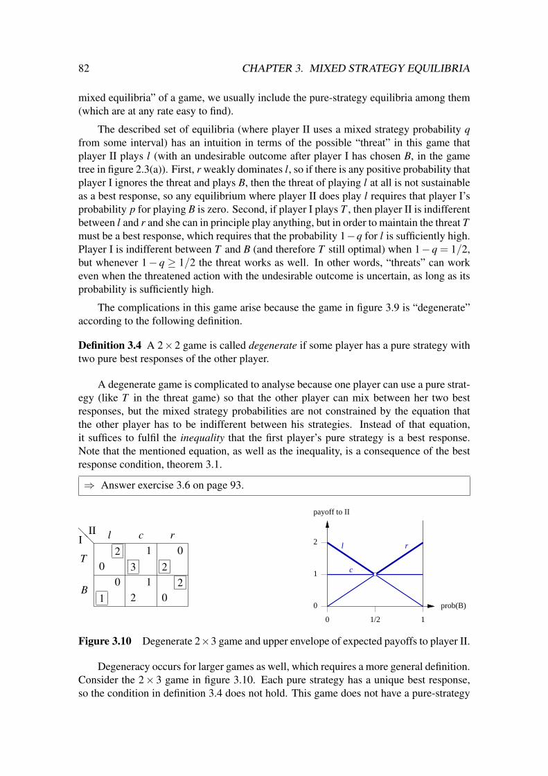
82 CHAPTER 3. MIXED STRATEGY EQUILIBRIA
mixed equilibria” of a game, we usually include the pure-strategy equilibria among them(which are at any rate easy to find).
The described set of equilibria (where player II uses a mixed strategy probability qfrom some interval) has an intuition in terms of the possible “threat” in this game thatplayer II plays l (with an undesirable outcome after player I has chosen B, in the gametree in figure 2.3(a)). First, r weakly dominates l, so if there is any positive probability thatplayer I ignores the threat and plays B, then the threat of playing l at all is not sustainableas a best response, so any equilibrium where player II does play l requires that player I’sprobability p for playing B is zero. Second, if player I plays T , then player II is indifferentbetween l and r and she can in principle play anything, but in order to maintain the threat Tmust be a best response, which requires that the probability 1−q for l is sufficiently high.Player I is indifferent between T and B (and therefore T still optimal) when 1−q = 1/2,but whenever 1− q ≥ 1/2 the threat works as well. In other words, “threats” can workeven when the threatened action with the undesirable outcome is uncertain, as long as itsprobability is sufficiently high.
The complications in this game arise because the game in figure 3.9 is “degenerate”according to the following definition.
Definition 3.4 A 2×2 game is called degenerate if some player has a pure strategy withtwo pure best responses of the other player.
A degenerate game is complicated to analyse because one player can use a pure strat-egy (like T in the threat game) so that the other player can mix between her two bestresponses, but the mixed strategy probabilities are not constrained by the equation thatthe other player has to be indifferent between his strategies. Instead of that equation,it suffices to fulfil the inequality that the first player’s pure strategy is a best response.Note that the mentioned equation, as well as the inequality, is a consequence of the bestresponse condition, theorem 3.1.
⇒ Answer exercise 3.6 on page 93.
@@I
II
T
B
l c r
0 3 22 1 0
1 2 00 1 2
1
2
1
0 prob(B)
1/2
payoff to II
0
c
l r
Figure 3.10 Degenerate 2×3 game and upper envelope of expected payoffs to player II.
Degeneracy occurs for larger games as well, which requires a more general definition.Consider the 2× 3 game in figure 3.10. Each pure strategy has a unique best response,so the condition in definition 3.4 does not hold. This game does not have a pure-strategy
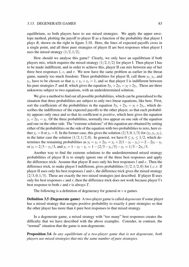
3.13. DEGENERATE GAMES 83
equilibrium, so both players have to use mixed strategies. We apply the upper enve-lope method, plotting the payoff to player II as a function of the probability that player Iplays B, shown on the right in figure 3.10. Here, the lines of expected payoffs cross ina single point, and all three pure strategies of player II are best responses when player Iuses the mixed strategy (1/2,1/2).
How should we analyse this game? Clearly, we only have an equilibrium if bothplayers mix, which requires the mixed strategy (1/2,1/2) for player I. Then player I hasto be made indifferent, and in order to achieve this, player II can mix between any of herthree best responses l, c, and r. We now have the same problem as earlier in the threatgame, namely too much freedom: Three probabilities for player II, call them yl , yc, andyr, have to be chosen so that yl + yc + yr = 1, and so that player I is indifferent betweenhis pure strategies T and B, which gives the equation 3yc +2yr = yl +2yc. These are threeunknowns subject to two equations, with an underdetermined solution.
We give a method to find out all possible probabilities, which can be generalised to thesituation that three probabilities are subject to only two linear equations, like here. First,sort the coefficients of the probabilities in the equation 3yc + 2yr = yl + 2yc, which de-scribes the indifference of the expected payoffs to the other player, so that each probabil-ity appears only once and so that its coefficient is positive, which here gives the equationyc +2yr = yl . Of the three probabilities, normally two appear on one side of the equationand one on the other side. The “extreme solutions” of this equation are obtained by settingeither of the probabilities on the side of the equation with two probabilities to zero, here ei-ther yc = 0 or yr = 0. In the former case, this gives the solution (2/3,0,1/3) for (yl,yc,yr),in the latter case the solution (1/2,1/2,0). In general, we have 0 ≤ yc ≤ 1/2, which de-termines the remaining probabilities as yl = yc +2yr = yc +2(1− yl− yc) = 2−2yl− ycor yl = 2/3− yc/3, and yr = 1− yl− yc = 1− (2/3− yc/3)− yc = 1/3−2yc/3.
Another way to find the extreme solutions to the underdetermined mixed strategyprobabilities of player II is to simply ignore one of the three best responses and applythe difference trick: Assume that player II uses only his best responses l and c. Then thedifference trick, to make player I indifferent, gives probabilities (1/2,1/2,0) for l,c,r. Ifplayer II uses only his best responses l and r, the difference trick gives the mixed strategy(2/3,0,1/3). These are exactly the two mixed strategies just described. If player II usesonly his best responses c and r, then the difference trick does not work because player I’sbest response to both c and r is always T .
The following is a definition of degeneracy for general m×n games.
Definition 3.5 (Degenerate game) A two-player game is called degenerate if some playerhas a mixed strategy that assigns positive probability to exactly k pure strategies so thatthe other player has more than k pure best responses to that mixed strategy.
In a degenerate game, a mixed strategy with “too many” best responses creates thedifficulty that we have described with the above examples. Consider, in contrast, the“normal” situation that the game is non-degenerate.
Proposition 3.6 In any equilibrium of a two-player game that is not degenerate, bothplayers use mixed strategies that mix the same number of pure strategies.

84 CHAPTER 3. MIXED STRATEGY EQUILIBRIA
⇒ You are asked to give the easy and instructive proof of proposition 3.6 in exercise 3.7on page 93.
In other words, in a non-degenerate game we have pure-strategy equilibria (both play-ers use exactly one pure strategy), or mixed-strategy equilibria where both players mixbetween exactly two strategies, or equilibria where both player mix between exactly threestrategies, and so on. In general, both players mix between exactly k pure strategies. Eachof these strategies has a probability, and these probabilities are subject to k equations inorder to make the other player indifferent between his or her pure strategies: One of theseequations states that the probabilities sum to one, and the other k− 1 equations state theequality between the first and second, second and third, etc., up to the (k− 1)st and kthstrategy of the other player. These equations have unique solutions. (It can be shown thatnon-unique solutions can occur only in a degenerate game.) These solutions have to bechecked for the equilibrium property: The resulting probabilities have to be non-negative,and the unused pure strategies of the other player must not have a higher payoff. Find-ing mixed strategy probabilities by equating the expected payoffs to the other player nolonger gives unique solutions in degenerate games, as we have demonstrated.
Should we or should we not care about degenerate games? In a certain sense, degen-erate games can be ignored when considering games that are given in strategic form, andwhere each cell of the payoff table arises from a different circumstance of the interactivesituation that is modelled by the game. In that case, it is “unlikely” that two payoffs areidentical, which is necessary to get two pure best responses to a pure strategy, which is theonly case where a 2×2 game can be degenerate. A small change of the payoff will resultin a unique preference of the other player. Similarly, it is unlikely that more than two linesdefining the upper envelope of expected payoffs cross in one point, or that more than threeplanes of expected payoffs against a mixed strategy that mixes three pure strategies (likein the two planes in figure 3.8) cross in one point, and so on. In other words, “generic” (or“almost all”) games in strategic form are not degenerate. On the other hand, degeneracyis very likely when looking at a game tree, because a payoff of the game tree will occurrepeatedly in the strategic form, as demonstrated by the threat game.
We conclude with a useful proposition that can be used when looking for all equi-libria of a degenerate game. In the threat game in figure 3.9, there are two equilib-ria ((1,0),(1,0)) and ((1,0),(1/2,1/2)) that are obtained, essentially, by “ignoring”the degeneracy. These two equilibria have the same strategy (1,0) of player I. Sim-ilarly, the game in figure 3.10 has two mixed equilibria ((1/2,1/2),(1/2,1/2,0)) and((1/2,1/2),(2/3,0,1/3)), which again share the same strategy of player I. The follow-ing proposition states that two mixed equilibria that have the same strategy of one player(here stated for player I, but it holds similarly for the other player) can be combined byconvex combinations to obtain further equilibria, as it is the case in the above examples.
Proposition 3.7 Consider a bimatrix game (A,B) with X as the set of mixed strategies ofplayer I, and Y as the set of mixed strategies of player II. Suppose that (x,y) and (x′,y)are equilibria of the game, where x,x′ ∈ X and y ∈ Y . Then ((1− p)x+ px′),y) is also anequilibrium of the game, for any p ∈ [0,1].

3.14. ZERO-SUM GAMES 85
Proof. Let x = (1− p)x + px′. Clearly, x ∈ X because xi ≥ 0 for all pure strategies i ofplayer I, and
m
∑i=1
xi =m
∑i=1
((1− p)xi + px′i) = (1− p)m
∑i=1
xi + pm
∑i=1
x′i = (1− p)+ p = 1.
The pair (x,y) is an equilibrium if x is a best response to y and vice versa. For anymixed strategy x of player I, we have xAy≥ xAy, and x′Ay≥ xAy, and consequently xAy =((1− p)x+ px′)Ay = (1− p)xAy+ px′Ay≥ (1− p)xAy+ pxAy = xAy, which shows that xis a best response to y. In other words, these inequalities hold because they are preservedunder convex combinations. In a similar way, y is a best response to x and x′, that is, forany y∈Y we have xBy≥ xBy and x′By≥ x′By. Again, taking convex combinations showsxBy≥ xBy.
We come back to the example of figure 3.10 to illustrate proposition 3.7: This gamehas two equilibria (x,y) and (x,y′) where x = (1/2,1/2), y = (1/2,1/2,0), and y′ =(2/3,0,1/3), so this is the situation of proposition 3.7, except that the two equilibria havesame mixed strategy of player I rather than player II. Consequently, for any y which is aconvex combination of y and y′ we have a Nash equilibrium (x,y). The equilibria (x,y)and (x,y′) are “extreme” in the sense that y and y′ have as many zero probabilities aspossible, which means that y and y′ are the endpoints of the line segment consisting ofequilibrium strategies y (that is, (x,y) is an equilibrium), where y = (1− p)y+ py′.
⇒ Express the set of Nash equilibria for the threat game in figure 3.9 with the help ofproposition 3.7.
3.14 Zero-sum games
Zero-sum games are games of two players where the interests of the two players aredirectly opposed: One player’s loss is the other player’s gain. Competitions betweentwo players in sports or in parlor games can be thought of as zero-sum games. Thecombinatorial games studied in chapter 1 are also zero-sum games.
Consider a zero-sum game in strategic form. If the row player chooses row i andthe column player chooses column j, then the payoff a(i, j) to the row player can beconsidered as a cost to the column player which she tries to minimise. That is, her payoffis given by b(i, j) = −a(i, j), that is, a(i, j)+ b(i, j) = 0, which explains the term “zero-sum”. The zero-sum game is completely specified by the matrix A with entries a(i, j)of payoffs to the row player, and the game is therefore often called a matrix game. Inprinciple, such a matrix game is a special case of a bimatrix game (A,B), where thecolumn player’s payoff matrix is B = −A. Consequently, we can analyse matrix gamesjust like bimatrix games. However, zero-sum games have additional strong properties,which are the subject of this section, that do not hold for general bimatrix games.
Figure 3.11 shows the football penalty kick as a zero-sum game between striker andgoalkeeper. For simplicity, assume that the striker’s possible strategies are L and R, that is,

86 CHAPTER 3. MIXED STRATEGY EQUILIBRIA
L w
l r
R
Figure 3.11 Strategic options for striker and goalkeeper in a football penalty.
to kick into the left or right corner, and that the goalkeeper’s strategies are l, w, r, where land r mean that he jumps immediately into the left or right corner, respectively, and w thathe waits and sees where the ball goes and jumps afterwards. On the left in figure 3.12,we give an example of resulting probabilities that the striker scores a goal, dependingon the choices of the two players. Clearly, the striker (player I) tries to maximise and thegoalkeeper (player II) to minimise that probability, and we only need this payoff to player Ito specify the game. The two players in a zero-sum game are therefore often called“Max” and “min”, respectively (where we keep our tradition of using lower case lettersfor the column player). In reality, one would expect higher scoring probabilities when thegoalkeeper chooses w, but the given numbers lead to a more interesting equilibrium. Inthis case, the striker does not score particularly well, especially when he kicks into theright corner.
@@
Maxmin
L
R
l w r
0.5 0.7 1.0
1.0 0.6 0.4
1
0 prob(R)
0
payoff to Max, = cost to min
0.70.60.50.4
3/5= 1/3x
1.0
lw
r
Figure 3.12 Left: the football penalty as a zero-sum game with scoring probabilities aspayoffs to the striker (row player), which the goalkeeper (column player)tries to minimise. Right: lower envelope of best response costs to the min-imiser.
In the payoff table in figure 3.12, we have indicated the pure best responses with littleboxes, in the lower left for the row player and in the upper right for the column player,similar to the boxes put around the payoffs in a bimatrix game when each cell has two
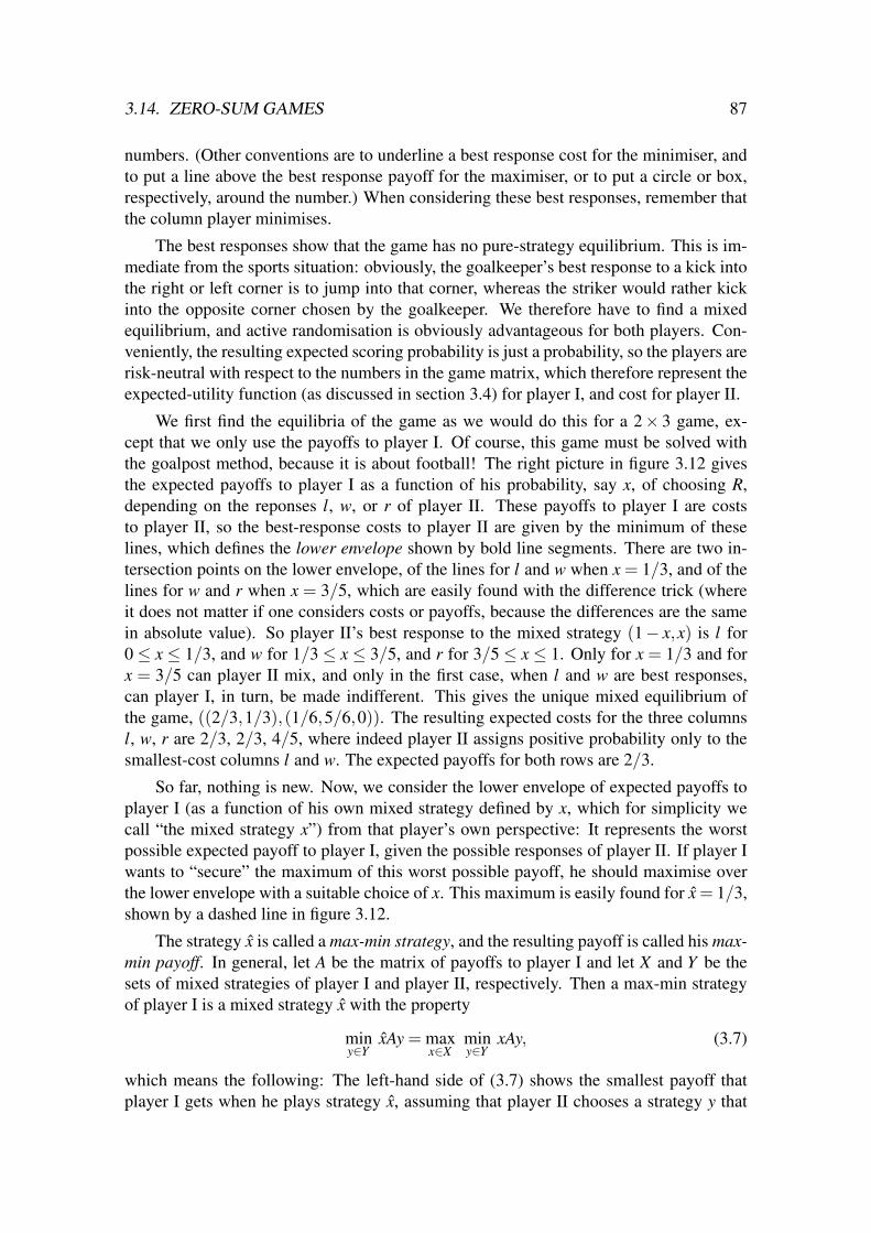
3.14. ZERO-SUM GAMES 87
numbers. (Other conventions are to underline a best response cost for the minimiser, andto put a line above the best response payoff for the maximiser, or to put a circle or box,respectively, around the number.) When considering these best responses, remember thatthe column player minimises.
The best responses show that the game has no pure-strategy equilibrium. This is im-mediate from the sports situation: obviously, the goalkeeper’s best response to a kick intothe right or left corner is to jump into that corner, whereas the striker would rather kickinto the opposite corner chosen by the goalkeeper. We therefore have to find a mixedequilibrium, and active randomisation is obviously advantageous for both players. Con-veniently, the resulting expected scoring probability is just a probability, so the players arerisk-neutral with respect to the numbers in the game matrix, which therefore represent theexpected-utility function (as discussed in section 3.4) for player I, and cost for player II.
We first find the equilibria of the game as we would do this for a 2× 3 game, ex-cept that we only use the payoffs to player I. Of course, this game must be solved withthe goalpost method, because it is about football! The right picture in figure 3.12 givesthe expected payoffs to player I as a function of his probability, say x, of choosing R,depending on the reponses l, w, or r of player II. These payoffs to player I are coststo player II, so the best-response costs to player II are given by the minimum of theselines, which defines the lower envelope shown by bold line segments. There are two in-tersection points on the lower envelope, of the lines for l and w when x = 1/3, and of thelines for w and r when x = 3/5, which are easily found with the difference trick (whereit does not matter if one considers costs or payoffs, because the differences are the samein absolute value). So player II’s best response to the mixed strategy (1− x,x) is l for0 ≤ x ≤ 1/3, and w for 1/3 ≤ x ≤ 3/5, and r for 3/5 ≤ x ≤ 1. Only for x = 1/3 and forx = 3/5 can player II mix, and only in the first case, when l and w are best responses,can player I, in turn, be made indifferent. This gives the unique mixed equilibrium ofthe game, ((2/3,1/3),(1/6,5/6,0)). The resulting expected costs for the three columnsl, w, r are 2/3, 2/3, 4/5, where indeed player II assigns positive probability only to thesmallest-cost columns l and w. The expected payoffs for both rows are 2/3.
So far, nothing is new. Now, we consider the lower envelope of expected payoffs toplayer I (as a function of his own mixed strategy defined by x, which for simplicity wecall “the mixed strategy x”) from that player’s own perspective: It represents the worstpossible expected payoff to player I, given the possible responses of player II. If player Iwants to “secure” the maximum of this worst possible payoff, he should maximise overthe lower envelope with a suitable choice of x. This maximum is easily found for x = 1/3,shown by a dashed line in figure 3.12.
The strategy x is called a max-min strategy, and the resulting payoff is called his max-min payoff. In general, let A be the matrix of payoffs to player I and let X and Y be thesets of mixed strategies of player I and player II, respectively. Then a max-min strategyof player I is a mixed strategy x with the property
miny∈Y
xAy = maxx∈X
miny∈Y
xAy, (3.7)
which means the following: The left-hand side of (3.7) shows the smallest payoff thatplayer I gets when he plays strategy x, assuming that player II chooses a strategy y that

88 CHAPTER 3. MIXED STRATEGY EQUILIBRIA
minimises player I’s payoff. The right-hand side of (3.7) gives the largest such “worst-case” payoff over all possible choices of x. The equality in (3.7) states that x is the strategyof player I that achieves this best possible worst-case payoff. It is therefore also sometimescalled a security strategy of player I, because it defines what player I can secure to get (interms of expected payoffs).
As a side observation, it is easy to see that the payoff miny∈Y xAy which describes the“worst case” payoff to player I when he plays x can be obtained by only looking at thepure strategies, the columns j, of player II. In other words, miny∈Y xAy = min j(xA) j. Thereason is that with a mixed strategy y, player II cannot produce a worse expected payoffto player I than with a pure strategy j, because the expectation represents a “weightedaverage” of the pure-strategy payoffs (xA) j with the probabilities y j as weights, so it isnever worse than the smallest of these pure-strategy payoffs (which is proved in the sameway as the best-response condition theorem 3.1). However, we keep the minimisationover all mixed strategies y in (3.7) because we will later exchange taking the maximumand the minimum. For player I, the max-min strategy x is better if he can use a mixedstrategy, as the football penalty game shows: If he was restricted to playing pure strategiesonly, his (pure-strategy) max-min payoff maxi min j a(i, j) would be 0.5, with pure max-min strategy L, rather than the max-min payoff 2/3 when he is allowed to use a mixedstrategy.
The max-min payoff in (3.7) is well defined and does not depend on what player IIdoes, because we always take the minimum over player II’s choices y. The functionminy∈Y xAy is a continuous function of x, and x is taken from the compact set X , so thereis some x where the maximum maxx∈X miny∈Y xAy of that function is achieved. The max-imum (and thus the max-min payoff) is unique, but there may be more than one choiceof x, for example if in the game in figure 3.12, the payoff 0.7 for the strategy pair (L,w)was replaced by 0.6, in which case the lower envelope would have its maximum 0.6 alongan interval of probabilities that player I chooses R, with any x in that interval defining amax-min strategy.
Recall how the max-min strategy x is found graphically over the lower envelope ofexpected payoffs. The max-min strategy x identifies the “peak” of that lower envelope.The “hat” accent x may be thought of as representing that peak.
⇒ Try exercise 3.8 on page 93, which is a variant of the football penalty game.
A max-min strategy, and the max-min payoff, only depends on the player’s own pay-offs. It can therefore also be defined for a game with general payoffs which are not nec-essarily zero-sum. In that case, a max-min strategy represents a rather pessimistic viewof the world: Player I chooses a strategy x that maximises his potential loss against anopponent who has nothing else on her mind than harming player I. In a zero-sum game,however, that view is eminently rational: Player II is not trying to harm player I, but sheis merely trying to maximise her own utility. This is because her payoffs are directlyopposed those of player I, her payoff matrix being given by B = −A. So the expressionminy∈Y xAy in (3.7) can also be written as −maxy∈Y xBy which is the (negative of the)best response payoff to player II. This is exactly what player II tries to do when maximis-ing her payoff against the strategy x of player I. As described above, the lower envelope

3.14. ZERO-SUM GAMES 89
of payoffs to player I is just the negative of the upper envelope of payoffs to player II,which defines her best responses.
So a max-min strategy is a natural strategy to look at when studying a zero-sum game.Our goal is now to show that in a zero-sum game, a max-min strategy is the same as anequilibrium strategy. This has some striking consequences, for example the uniquenessof the equilibrium payoff in any equilibrium of a zero-sum game, which we will discuss.
We consider such a max-min strategy not only for player I but also for player II,whose payoff matrix is B =−A. According to (3.7), this is a mixed strategy y of player IIwith the property
minx∈X
xBy = maxy∈Y
minx∈X
xBy,
which we re-write as−max
x∈XxAy =−min
y∈Ymaxx∈X
xAy
or, omitting the minus signs,
maxx∈X
xAy = miny∈Y
maxx∈X
xAy. (3.8)
Equation (3.8) expresses everything in terms of a single matrix A of payoffs to player I,which are costs to player II that she tries to minimise. In order to simplify the discussion ofthese strategies, a max-min strategy of player II (in terms of her own payoffs) is thereforealso called a min-max strategy (with the min-max understood in terms of her own costs,which are the payoffs to her opponent). So a min-max strategy of player II is a strategyy that minimises the worst-case cost maxx∈X xAy that she has to pay to player I, as statedin (3.8).
The first simple relationship between the max-min payoff to player I in a zero-sumgame and the min-max cost to player II is
maxx∈X
miny∈Y
xAy≤miny∈Y
maxx∈X
xAy. (3.9)
The left-hand side is the “secure” payoff that player I can guarantee to himself (on aver-age) when using a max-min strategy x, the right-hand side the “secure” cost that player IIcan guarantee to herself to pay at most (on average) when using a min-max strategy y. Itis clear that this is the only direction in which the inequality can hold if that “guarantee”is to be meaningful. For example, if player I could guarantee to get a payoff of 10, andplayer II could guarantee to pay at most 5, something would be wrong. The proof of (3.9)is similarly simple:
maxx∈X
miny∈Y
xAy = miny∈Y
xAy≤ xAy≤maxx∈X
xAy = miny∈Y
maxx∈X
xAy.
The main theorem on zero-sum games states the equation “max min = min max”, tobe understood for the payoffs, that is, equality instead of an inequality in (3.9). This isalso called the “minimax” theorem, and it is due to von Neumann.
The next theorem clarifies the connection between max-min strategies (which forplayer II we called min-max strategies) and the concept of Nash equilibrium strategies.Namely, for zero-sum games they are the same. Furthermore, the existence of a Nashequilibrium strategy pair (x∗,y∗) implies the minimax theorem, that is, equality in (3.9).

90 CHAPTER 3. MIXED STRATEGY EQUILIBRIA
Theorem 3.8 (von Neumann’s minimax theorem) Consider a zero-sum game with pay-off matrix A to player I. Let X and Y be the sets of mixed strategies of player I and II,respectively, and let (x∗,y∗) ∈ X×Y . Then (x∗,y∗) is a Nash equilibrium if and only if x∗is a max-min strategy and y∗ is a min-max strategy, that is,
miny∈Y
x∗Ay = maxx∈X
miny∈Y
xAy, maxx∈X
xAy∗ = miny∈Y
maxx∈X
xAy. (3.10)
Furthermore,maxx∈X
miny∈Y
xAy = miny∈Y
maxx∈X
xAy. (3.11)
Proof. Consider a max-min strategy x in X and a min-max strategy y in Y , which fulfil(3.10) in place of x∗ and y∗, respectively. Such strategies exist because X and Y arecompact sets. Let (x∗,y∗) be any Nash equilibrium of the game, which exists by Nash’stheorem 3.3. The equilibrium property is equivalent to the “saddle point” property
maxx∈X
xAy∗ = x∗Ay∗ = miny∈Y
x∗Ay, (3.12)
where the left equation states that x∗ is a best response to y∗ and the right equation statesthat y∗ is a best response to x∗ (recall that B = −A, so player II tries to minimise herexpected costs xAy). Then
xAy≤maxx∈X
xAy = miny∈Y
maxx∈X
xAy≤maxx∈X
xAy∗ = x∗Ay∗ (3.13)
andxAy≥min
y∈YxAy = max
x∈Xminy∈Y
xAy≥miny∈Y
x∗Ay = x∗Ay∗, (3.14)
so all these inequalities hold as equalities. With the second inequality in both (3.13) and(3.14) as an equality we get (3.10), that is, y∗ is a min-max and x∗ is a max-min strategy.Having the first inequality in both (3.13) and (3.14) as an equality gives
maxx∈X
xAy = xAy = miny∈Y
xAy,
which says that (x, y) is a Nash equilibrium. Furthermore, we obtain (3.11).
One consequence of theorem 3.8 is that in any Nash equilibrium of a zero-sum game,a player receives the same payoff, namely the max-min payoff to player I in (3.11), whichis the min-max cost to player II. This payoff is also called the value of the zero-sum game.
Another important consequence of the theorem 3.8 is that the concept of “Nash equi-librium strategy” in a zero-sum game is independent of what the opponent does, becauseit is the same as a max-min strategy (when considered in terms of the player’s own pay-offs). This is far from being the case in general-payoff games, as, for example, the gameof “chicken” demonstrates. In particular, if player I’s strategies x∗ and x are both part ofa Nash equilibrium in a zero-sum game, they are part of any Nash equilibrium. So Nashequilibrium strategies are interchangeable: if (x∗,y∗) and (x,y) are Nash equilibria, so are(x∗,y) and (x,y∗). The reason is that x∗ and x are then max-min strategies, and y∗ and yare min-max strategies, which has nothing to do with what the opponent does.

3.15. EXERCISES FOR CHAPTER 3 91
A further consequence is that if (x∗,y∗) is a Nash equilibrium and y∗ is the unique bestresponse (for example, this is often the case when y∗ is a pure strategy), then y∗ is also theunique min-max strategy. The reason is that if there was another min-max strategy y thatis different from y∗, then (x∗, y) would be a Nash equilibrium, and consequently y wouldbe a best response to x∗, contradicting the uniqueness of the best response y∗. Similarly,if, say, x is the unique max-min strategy of player I (for example, obtained by plotting thelower envelope against x as in figure 3.12), it is also the only Nash equilibrium strategyof player I.
These properties of zero-sum games make equilibrium strategies, or equivalentlymax-min/min-max strategies, a particularly convincing solution concept. They are alsocalled “optimal” strategies for the players.
3.15 Exercises for chapter 3
Exercise 3.1 shows how to find all mixed equilibria of a small bimatrix game, which ishowever not a 2×2 game. It is useful to attempt this exercise as early as possible, becausethis will help you appreciate the methods developed later. The given solution to this exer-cise does not use the upper envelope method, but you should try using that method onceyou have learned it; it will help you solve the exercise faster. Exercise 3.2 is a (not easy)continuation of exercise 2.7, and asks about mixed equilibria in a three-player game tree.In exercise 3.3, you are asked to derive the “difference trick”. Exercise 3.4 demonstratesthe power of the upper envelope method for 2× n games. In exercise 3.5, you shouldunderstand the concept of dominated strategies with the help of of the upper-envelopediagram, which provides a useful geometric insight. A degenerate game is treated in ex-ercise 3.6. Exercise 3.7 shows that in non-degenerate games, Nash equilibria are alwaysplayed on square games that are part of the original game, in the sense that both playersmix between the same number of pure strategies. Exercise 3.8 is a variant of the footballpenalty.
Exercise 3.1 Find all Nash equilibria of the following 3× 2 game, including equilibriaconsisting of mixed strategies.
@@@I
II
T
M
B
l r
0 6
1 0
2 5
0 2
3 3
3 4
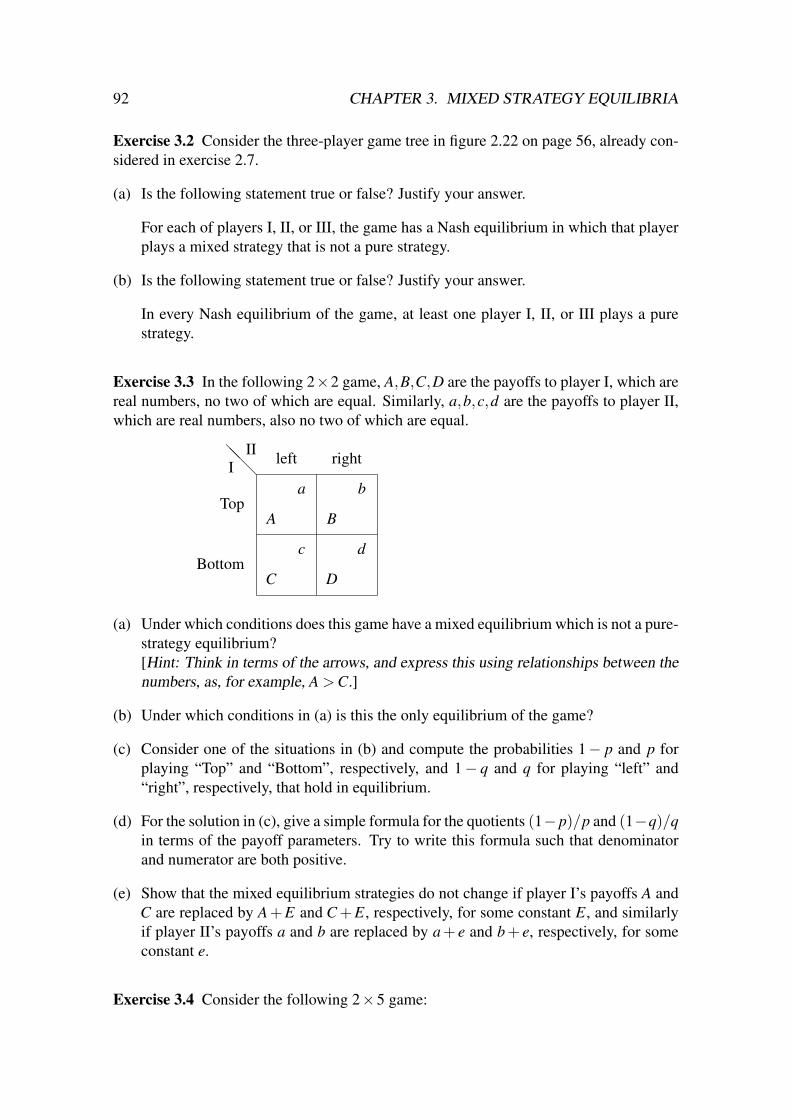
92 CHAPTER 3. MIXED STRATEGY EQUILIBRIA
Exercise 3.2 Consider the three-player game tree in figure 2.22 on page 56, already con-sidered in exercise 2.7.
(a) Is the following statement true or false? Justify your answer.
For each of players I, II, or III, the game has a Nash equilibrium in which that playerplays a mixed strategy that is not a pure strategy.
(b) Is the following statement true or false? Justify your answer.
In every Nash equilibrium of the game, at least one player I, II, or III plays a purestrategy.
Exercise 3.3 In the following 2×2 game, A,B,C,D are the payoffs to player I, which arereal numbers, no two of which are equal. Similarly, a,b,c,d are the payoffs to player II,which are real numbers, also no two of which are equal.
@@@I
II
Top
Bottom
left right
A B
a b
C D
c d
(a) Under which conditions does this game have a mixed equilibrium which is not a pure-strategy equilibrium?[Hint: Think in terms of the arrows, and express this using relationships between thenumbers, as, for example, A > C.]
(b) Under which conditions in (a) is this the only equilibrium of the game?
(c) Consider one of the situations in (b) and compute the probabilities 1− p and p forplaying “Top” and “Bottom”, respectively, and 1− q and q for playing “left” and“right”, respectively, that hold in equilibrium.
(d) For the solution in (c), give a simple formula for the quotients (1− p)/p and (1−q)/qin terms of the payoff parameters. Try to write this formula such that denominatorand numerator are both positive.
(e) Show that the mixed equilibrium strategies do not change if player I’s payoffs A andC are replaced by A + E and C + E, respectively, for some constant E, and similarlyif player II’s payoffs a and b are replaced by a + e and b + e, respectively, for someconstant e.
Exercise 3.4 Consider the following 2×5 game:

3.15. EXERCISES FOR CHAPTER 3 93
@@@I
II
T
B
a b c d e
0 2 1 0 3
2 4 3 5 0
1 0 4 1 0
7 4 5 0 8
(a) Draw the expected payoffs to player II for all her strategies a,b,c,d,e, in terms ofthe probability p, say, that player I plays strategy B. Indicate the best responses ofplayer II, depending on that probability p.
(b) Using the diagram in (a), find all pure or mixed equilibria of the game.
Exercise 3.5 Consider the quality game in figure 2.10.
(a) Use the “goalpost” method twice, to draw the upper envelope of best-response pay-offs to player I against the mixed strategy of player II, and vice versa.
(b) Explain which of these diagrams shows that a pure strategy dominates another purestrategy.
(c) Explain how that diagram shows that if a strategy s dominates a strategy t, then t isnever a best response, even against a mixed strategy of the other player.
Exercise 3.6 Find all equilibria of the following degenerate game, which is a variant ofthe inspection game in figure 3.2. The difference is that player II, the inspectee, derivesno gain from acting illegally (playing r) even if she is not inspected (player I choosing T ).
@@@I
II
T
B
l r
0 −10
0 0
−1 −6
0 −90
Exercise 3.7 Prove proposition 3.6.
Exercise 3.8 Consider the duel in a football penalty kick. The following table describesthis as a zero-sum game. It gives the probability of scoring a goal when the row player(the striker) adopts one of the strategies L (shoot left), R (shoot right), and the columnplayer (the goalkeeper) uses the strategies l (jump left), w (wait then jump), r (jumpright). The row player is interested in maximising and the column player in minimisingthe probability of scoring a goal.

94 CHAPTER 3. MIXED STRATEGY EQUILIBRIA
@@@
Maxmin
L
R
l w r
0.6 0.7 1.0
1.0 0.8 0.7
(a) Find an equilibrium of this game in pure or mixed strategies, and the equilibriumpayoff. Why is the payoff unique?
(b) Now suppose that player I has an additional strategy M (shoot in the middle), so thatthe payoff matrix is
@@@
Maxmin
L
R
M
l w r
0.6 0.7 1.0
1.0 0.8 0.7
1.0 0.0 1.0
Find an equilibrium of this game, and the equilibrium payoff.[Hint: The result from (a) will be useful.]

Chapter 4
Game trees with imperfect information
This chapter studies extensive games, which are game trees with imperfect information.It relies on chapters 2 and 3.
4.1 Learning objectives
After studying this chapter, you should be able to:
• explain extensive games and the concept of information sets;
• describe pure and reduced pure strategies for extensive games, and the correspondingstrategic form and reduced strategic form of the game;
• define the concept of perfect recall, and see if this holds for a given game;
• explain the difference between behaviour and mixed strategies, and state Kuhn’s the-orem;
• construct simple extensive games from descriptions of games with imperfect infor-mation, like the game in exercise 4.3 on page 123;
• find all equilibria of simple extensive games, and represent the mixed strategies inthese equilibria as behaviour strategies.
4.2 Further reading
Extensive games with imperfect information are a standard concept in game theory. Theyare treated here in greater detail than elsewhere, in particular as concerns information setsand the condition of perfect recall.
One alternative reference is chapter 11 of
• Osborne, Martin J., and Ariel Rubinstein A Course in Game Theory. (MIT Press,1994) [ISBN 0262650401].
A short treatment of extensive games is given in section 2.4 of
95

96 CHAPTER 4. GAME TREES WITH IMPERFECT INFORMATION
• Gibbons, Robert A Primer in Game Theory [in the United States sold under the titleGame Theory for Applied Economists]. (Prentice Hall / Harvester Wheatsheaf, 1992)[ISBN 0745011594].
Information sets were introduced by Harold Kuhn in the following article:
• Kuhn, Harold W. “Extensive games and the problem of information”, in: Contri-butions to the Theory of Games II, eds. H. W. Kuhn and A. W. Tucker, Annals ofMathematics Studies, Vol. 28 (1953), Princeton Univ. Press, pp. 193–216.
The “Annals of Mathematics Studies” where this article appeared is a book series.Kuhn’s article defines perfect recall in a way that is not, at first glance, the same as here,but it should be possible to understand that the definitions are the same after having stud-ied this chapter. The definition 4.1 of perfect recall that we give is due to the followingarticle by Reinhard Selten.
• Selten, Reinhard “Reexamination of the perfectness concept for equilibrium points inextensive games”, International Journal of Game Theory, Vol. 4 (1975), pp. 25–55.
4.3 Introduction
Typically, players do not always have full access to all the information which is relevantto their choices. Extensive games with imperfect information model exactly what infor-mation is available to the players when they make a move. Modelling and evaluatingstrategic information precisely is one of the strengths of game theory.
The central concept of information sets is introduced in section 4.4 by means ofa detailed example. We then give the general definition of extensive games, and thedefinition of strategies and reduced strategies, which generalise these concepts as theyhave been introduced for game trees with perfect information. Essentially, all one has todo is to replace “decision node” by “information set”.
The concept of perfect recall states a condition on the structure of the informationsets of a player, which have to be in a certain sense “compatible” with the game tree.(Perfect recall is not about how to interpret the game.) The related concept of behaviourstrategies and Kuhn’s theorem is then studied in depth.
The final section 4.12 treats subgames and subgame perfect Nash equilibria (SPNE).
4.4 Information sets
Consider the situation faced by a large software company (player I) after a small startupfirm (player II) has announced deployment of a key new technology. The large companyhas a large research and development operation. It is generally known that they haveresearchers working on a wide variety of innovations. However, only the large companyknows for sure whether or not they have made any progress on a product similar to thestartup’s new technology. The startup believes that there is a 50 percent chance that the

4.4. INFORMATION SETS 97
large company has developed the basis for a strong competing product. For brevity, whenthe large company has the ability to produce a strong competing product, the companywill be referred to as having a “strong” position, as opposed to a “weak” one.
The large company, after the announcement by the small company, has two choices.It can counter by announcing that it too will release a competing product. Alternatively, itcan choose to cede the market for this product. The large company will certainly conditionits choice upon its private knowledge, and may choose to act differently when it has astrong position than when it has a weak one. If the large company has announced aproduct, the startup is faced with a choice: it can either negotiate a buyout and sell itselfto the large company, or it can remain independent and launch its product. The startupdoes not have access to the large firm’s private information on the status of its research.However, it does observe whether or not the large company announces its own product,and may attempt to infer from that choice the likelihood that the large company has madeprogress of its own.
When the large company does not have a strong product, the startup would prefer tostay in the market over selling out. When the large company does have a strong product,the opposite is true, and the startup is better off selling out instead of staying in.
20−44
12−4204
12
1600
16
DCBT
a b a b
II
II
chance
1/21/2
Figure 4.1 Game with imperfect information for player II, indicated by the informationset that contains two decision nodes with the same moves a and b. At a leafof the tree, the top payoff is to player I, the bottom payoff to player II (asalways).
Figure 4.1 shows a game tree with imperfect information (also called “extensivegame”) that models this situation. From the perspective of the startup, whether or notthe large company has done research in this area is random. This is here modelled byan initial chance move, where the left branch stands for a “weak” player I (as describedabove), and the right branch for a “strong” player I. Both branches have here probabil-ity 1/2.
When the large company is in a weak position, it can choose to cede the market tothe startup. This is given by move T , with payoffs (0,16) to the two players. It can

98 CHAPTER 4. GAME TREES WITH IMPERFECT INFORMATION
also announce a competing product, modeled by move B, in the hope that the startupcompany, player II, will sell out, choosing move a, with payoffs 12 and 4 to players Iand II. However, if player II decides instead to stay in the market (move b) it will evenprofit from the increased publicity and gain a payoff of 20, with a loss of −4 to player I.
In contrast, when player I is in a strong position, it can again cede the market toplayer II (move C, with the same payoff pair (0,16) as before), or instead announceits own product (move D). It will quickly become apparent that player I should neverchoose C, but we keep it as a possibility. After move D of the “strong” player I, thepayoffs to the two players are (12,4) if the startup sells out (move a) and (20,−4) if thestartup stays in (move b).
In addition to a game tree with perfect information, the nodes of the players are en-closed by ovals which define information sets. These are simply sets of decision nodes,subject to certain restrictions that we will describe shortly in generality. The interpreta-tion is that a player cannot distinguish among the nodes in an information set, given hisknowledge at the time he makes the move. Because his knowledge at all nodes in aninformation set is the same, he makes the same choice at each node in that set. Here, thestartup company, player II, must choose between move a (sell out) and move b (stay inthe market). These are the two choices at player II’s information set, which has two nodesaccording to the different histories of play, which player II cannot distinguish.
Because player II is not informed about her position in the game, backward inductioncan no longer be applied. If player II knew whether player I is in a weak or strongposition, then it would be better for her to choose b when facing a weak player I (leftnode in figure 4.1), and to choose a when facing a strong player I (right node of theinformation set).
One “optimal move” that can be seen directly from the game tree is the choice be-tween C or D of player I. Choosing C gives player I a payoff of zero, whereas D gives himeither 12 or 20, depending on whether player II chooses a or b. Both payoffs are largerthan zero, so player I should choose D at any rate. So the game reduces to a decisionbetween move T and B for player I, and between a and b for player II, assuming player Ialways chooses D.
The game tree shows that no pair of these moves for the two players is optimal againstthe other. For player I, if player II chooses b, then move T is better (because 0 is a higherpayoff than−4). If player I chooses T , then the left node of the information set of player IIis not reached. In that case, when player II has the choice between a and b, she knowswith certainty that she is at the right node of her information set. Hence, she gets thehigher payoff 4 when choosing a (rather than −4 when choosing b), that is, player II will“sell out” to the big company and choose move a. If player II, in turn, chooses a, thenplayer I’s choice between T and B is in favour of B, which gives the higher payoff 12compared to 0. If player I chooses B, then player II will be with equal probability at eitherthe left or the right node in her information set. Player II then has to use expected payoffswhen comparing a and b. Clearly, move a will give her payoff 4, whereas move b willgive her the expected payoff 1/2 ·20+1/2 · (−4) = 8. That expected payoff exceeds thepayoff for move a. That is, against B, player II is better off choosing b. We have now come

4.4. INFORMATION SETS 99
full circle: The sequence of best-response moves for the players is b→ T → a→ B→ b,so there is no deterministic behaviour of the players that defines an equilibrium.
The game in figure 4.1 can be analysed in terms of the moves alone (we will give suchan analysis at the end of this section), because for each player, only two choices matter;this follows from the initial separate consideration that excludes move C as a rationalchoice.
However, in general it is useful to consider the strategic form of the game that hasalready been considered for game trees with perfect information. This involves system-atically considering the strategies that players have in the game. The Nash equilibriumconcept is also defined in terms of strategies, and not in terms of moves.
@@@I
II
TC
T D
BC
BD
a b
0 0
16 16
6 10
10 6
6 −2
10 18
12 8
4 8
@@@I
II
T D
BD
a b
6 10
10 6
12 8
4 8
Figure 4.2 Strategic form of the game in figure 4.1 (left), and the 2×2 game (right) thatresults after eliminating the strictly dominated strategies TC and BC, withbest response payoffs.
The left table in figure 4.2 gives the strategic form of the game in figure 4.1. As inthe case of game trees with perfect information, a strategy of a player defines a movefor each of the player’s decision nodes. The difference, however, is that such a move isonly specified once for all the decision nodes that belong to an information set, becauseby definition the choice of that move is the same no matter where the player is in theinformation set. In figure 4.1, this means that player II has only two moves, which are thetwo moves a and b at her only information set. Because player II has only one informationset, her strategies are the same as her moves. Player I has two information sets, so astrategy for player I is a pair of moves, one move for the first and one move for the secondinformation set. These pairs of moves are TC,T D,BC,BD.
The four strategies of player I correspond to the rows on the left in figure 4.2, whereasthe columns are the strategies a and b of player II. Each of the eight cells in that table givesthe expected payoffs as they are calculated from the payoffs at the leaves and the chanceprobabilities. For example, the strategy pair (BC,a) gives expected payoff 1/2 · 12 +1/2 ·0 = 6 to player I and payoff 1/2 ·4 + 1/2 ·16 = 10 to player II. These expectations

100 CHAPTER 4. GAME TREES WITH IMPERFECT INFORMATION
come from the possible chance moves, both of which have probability 1/2 according tofigure 4.1. So when the chance move goes to the left, the strategy pair (BC,a) means theplay of the game follows move B and then move a, reaching the leaf with payoffs 12,4 toplayers I, II. When the chance move goes to the right, the strategy pair (BC,a) means thatmove C leads immediately to the leaf with payoffs 0,16.
The left 4× 2 game in figure 4.2 has two strictly dominated strategies, namely TC,which is strictly dominated by T D, and BC, which is strictly dominated by BD. Thisis in agreement with the earlier observation that for player I, move C is always worsethan move D, no matter what player II does. In a certain respect one has to be careful,though, to conclude that a “worse move” always leads to a strictly dominated strategy(the dominated strategy, for example TC instead of T D, would be obtained by replacinga given move, like D as part of the strategy T D, by the “worse move”, here C). Namely,even if the payoffs from the “worse move” (in the example C) are strictly worse than thoseresulting from the given move (D), one has to make sure that the decision point with themoves in question (C and D) is always reached with positive probability. (Only in thiscase the expected payoffs from the two strategies will always differ.) This is here the casebecause the decision point of player I with moves C and D is reached by a chance move.If, in contrast, the chance move was replaced by a move of a third player, for example,then if that third player does not move to the right, the choice between C and D wouldnot affect the payoff to player I. So in this case, we could only conclude that T D weaklydominates TC. In short, it is safer to look at the strategic form of the game, even thougha careful look at the game tree may eliminate some strategies right away.
Elimination of the strictly dominated strategies TC and BC gives the 2× 2 game onthe right in figure 4.2. There, each player has two strategies, which correspond to thetwo moves discussed earlier. The best response payoffs indicated by boxes show that thisgame has no pure-strategy equilibrium.
The equilibrium of the game involves both players randomising. The mixed strategyprobabilities can be determined in the familiar way. Player I randomises with equal prob-ability 1/2 between T D and BD so that the expected payoff to player II is 7 for both aand b. Conversely, player II chooses a with probability 1/4 and b with probability 3/4.Then player I is indifferent, receiving an overall expected payoff of 36/4 = 9 in each case.
The game in figure 4.1 is a competition between two firms that is more familiar whenviewed as a simple case of the card game poker. We can think of player I being dealt aweak or strong hand, which is with equal probability either worse or better than the handof player II (this is represented by the left and right chance move, respectively). Player Iknows whether his hand is weak or strong (in a real poker game, player I knows his handbut not necessarily whether it is better or worse than that of player II). Player I can theneither “fold” (moves T and C), or “raise” (moves B and D). In turn, player II can either“pass” (move a) or “meet”. The “fold” and “pass” moves entail a fixed outcome wherethe players receive payoffs that are independent of the hands they hold. Only the combi-nations of moves “raise” and “meet”, corresponding to the strategy pair (BD,b), lead tooutcomes where the players’ hands matter, as can be seen from figure 4.1 (the reason thatother strategy pairs give non-constant payoffs in figure 4.2 is due to the different effect ofthe chance move in each case).

4.4. INFORMATION SETS 101
We can say that when player I has a weak hand and decides to “raise” (move B),this amounts to bluffing, pretending that he has a strong hand, because player II does notknow this. The purpose of bluffing, however, is not only to make player II “pass”. Indeed,player II would not “pass” (move a) if player I bluffed all the time, as analysed before.One main effect of bluffing is to leave player II uncertain as to whether player I has astrong or weak hand. The best possible outcome for player I is if player II meets a stronghand of player I (moves D and b), because this gives player I maximum payoff. If player Iraises only if he has a strong hand, then player II would rather pass, which is not in theinterest of player I. Above, we have reasoned that no deterministic combination of movesleads to an equilibrium. As described, this is made very vivid in terms of the poker gameinterpretation.
To conclude the discussion of this example, we can also deduce in this case directlyfrom the game tree the probabilities for the moves T and B, and for a and b, that arenecessary in order to reach an equilibrium. Even without constructing the strategic form,we have seen that no deterministic choice of these moves gives an equilibrium. Hence,both players must randomise, and for that purpose they must be indifferent between theirchoices. For player I, this indifference is very easy to determine: If he has to decidebetween T and B, then he gets the certain payoff 0 with T , so indifference results onlywhen the expected payoff for B is also 0. If player II chooses a and b with probabilities1−q and q, respectively, that expected payoff to player I is 12(1−q)−4q, so the equation0 = 12(1−q)−4q = 12−16q determines uniquely q = 3/4.
In turn, player II has to be indifferent between her moves a and b in order to ran-domise in that way. Here the situation is somewhat more complicated, because the ex-pected payoff to player II depends on the probabilities of being either at the left or at theright node in her information set. Assuming, as we do, that player I makes the rationalchoice and chooses D with certainty, the probability of being at the right node is 1/2,whereas the probability of being at the left node is 1/2 · p, where p is the probability ofplayer I choosing B. Because there is a non-zero probability 1− p for T , the game endswith probability 1/2 · (1− p) at the leftmost leaf of the tree, and then the information setof player II will not be reached at all. Technically, what has to be computed is the con-ditional probability that player II will be at the left node versus being at the right node.Before going into the details, we note that from the description so far, the probability forthe left node is p times the probability for the right node. Only these relative weightsmatter. Indifference of player II between a and b then gives the following equation, withthe weighted payoffs for a and b on the left and right, respectively:
p ·4+1 ·4 = p ·20+1 · (−4), (4.1)
which simplifies to 4p+4 = 20p−4 or 8 = 16p, that is, p = 1/2.
The conditional probabilities for player II being at the left and right node are com-puted as follows: The left node has absolute probability 1/2 · p of being reached, the rightnode absolute probability 1/2. The total probability of being at any of the two nodes(which are disjoint events) is the sum of these two probabilities, namely (p + 1)/2. Theconditional probability is then the absolute probability divided by the total probability,that is, for the left node, p/2
(p+1)/2 or pp+1 , and for the right node, 1/2
(p+1)/2 or 1p+1 . Using

102 CHAPTER 4. GAME TREES WITH IMPERFECT INFORMATION
these conditional probabilities instead of the “weights” in (4.1) would mean dividing bothsides of equation (4.1) by p+1. The first step in solving that amended equation would beto multiply both sides by p + 1, giving back (4.1), so what we have done is perfectly inorder (as long as the total probability of reaching the information set in the first place isnonzero).
One more time, we interpret the equilibrium probabilities p = 1/2 and q = 3/4 interms of the game tree: Player I, by choosing B with probability 1/2, and D with certainty,achieves that player II is half as likely to be at the left node of her information set asat her right node. Therefore, the conditional probabilities for left versus right node are1/3 and 2/3, respectively (1/4 and 1/2 divided by the total probability 3/4 of reachingthe information set). Exactly in that case, player II is indifferent between a and b: Theconditional expected payoffs to player II are then (clearly) 4 for move a, and 1/3 · 20 +2/3 · (−4) = 12/3 = 4 for move b. The overall expected payoff to player II has to takethe absolute probabilities into account: With probability 1/4 (left chance move, player Ichoosing T ), she gets payoff 16, with probability 3/4, the mentioned conditional payoff 4,overall 1/4 · 16 + 3/4 · 4 = 4 + 3 = 7. For player I, we have observed the indifferencebetween T and B, so when the chance move goes to the left, player I gets payoff zero.When the chance move goes to the right, player I when choosing D will get (1−q) ·12+q ·20 = 1/4 ·12+3/4 ·20 = 18. The overall payoff to player I is 1/2 ·0+1/2 ·18 = 9.
4.5 Extensive games
In this section, we give the general definition of an extensive game, also known as a gamein extensive form, or as a game tree with imperfect information.
Similar to the game trees with perfect information considered earlier, the basic struc-ture of an extensive game is a tree. As before, it has three types of nodes: Terminal nodes,called leaves, with a payoff for each player; non-terminal nodes which are either chancenodes (typically drawn as squares), where the next node is chosen randomly accordingto a given probability that is specified in the tree, or non-terminal nodes that are decisionnodes, which belong to a particular player. The outgoing edges from each decision nodeare labelled with the names of choices or moves which uniquely identify the respectiveedges.
The decision nodes are partitioned into information sets. “Partitioned” means thatevery decision node belongs to exactly one information set, and no information set isempty. When drawing the extensive game, information sets are typically shown as ovalsaround the nodes that they contain; some people draw information sets by joining thenodes in the set with a single dashed line instead.
The interpretation of an information set is that in the course of the game, a player isonly told that he is at some node in an information set, but not at which particular node.Consequently, the information sets have to fulfil certain conditions: In an information set,all decision nodes belong to the same player; all decision nodes in the set have the samenumber of outgoing edges; and the set of moves (given by the labels on the outgoingedges) is the same for each node in the information set. In figure 4.1, for example, the

4.5. EXTENSIVE GAMES 103
information set of player II has two moves, a and b. When the player has reached aninformation set, he makes a choice by picking a move, which is by definition the samemove no matter where he is in the information set.
These conditions are trivially fulfilled if every information set is a singleton (containsonly one node). If all information sets are singletons, then the game has perfect infor-mation and the information sets could as well be omitted. This gives a game tree withperfect information as considered earlier. Only for information sets that contain two ormore nodes do these conditions matter.
chance
1/21/2
IR
L
L
R
0 2
1
3
Figure 4.3 Game with an information set where two nodes share a path, which is usuallynot allowed in an extensive game.
In addition to the above conditions, we will impose additional constraints on thestructure of the information sets. The first of these is that no two nodes in an informationset share a path, as in the example in figure 4.3. The single-player game in that figurehas two decision nodes of player I, which belong to a single information set that hasthe two moves L and R. The only other non-terminal node is a chance move. Everycondition about extensive games is met. However, the two decision nodes of player Ishare a path, because the first node is the root, from which there is a path to the secondnode. Information sets with this feature have a very problematic interpretation, becausewe require that a move, for example L, at such an information set is the same no matterwhere the player is. However, in figure 4.3, what would it mean for player I to makemove L? It certainly means going left from the root, but if afterwards the chance movegoes to the right so that player I can move again, does he automatically have to makemove L again?
The problem with the information set in figure 4.3 is that, by the interpretation ofinformation sets, player I must have forgotten if he made a move at all when called tochoose between L and R, and it is not even clear whether he is allowed to choose “again”or not. An information set can represent that a player forgets what he knew or did earlier.In that case, the player is said to have imperfect recall. However, players with imperfectrecall do not conform to our idea of “rational” players. Moreover, their forgetfulness isnot very adequately represented by information sets. We will therefore assume that allplayers have perfect recall, which is defined, and discussed in detail, in section 4.8 below.In particular, we will see that perfect recall implies that no two nodes in an informationset are connected by a path in the tree (see proposition 4.2 below), so that a situation likein figure 4.3 cannot occur.

104 CHAPTER 4. GAME TREES WITH IMPERFECT INFORMATION
To summarise the definition of game trees with imperfect information: The only newfeature added to the game tree is the concept of information sets, which model a player’slack of information about where he is in the game.
4.6 Strategies for extensive games and the strategic form
The definition of a strategy in an extensive game generalises the definition of a strategyfor a game tree with perfect information: A (pure) strategy of a player specifies a movefor each information set of the player.
A formal definition of strategies requires some notation to refer to the informationsets of a player, and the moves available at each information set. Suppose player i is aplayer in the extensive game (like player I or player II in a two-player game). Then Hidenotes the set of information sets of player i. A particular information set of player iis typically called h. We denote the set of choices or moves at the information set h byCh for h ∈ Hi. For example, if h is the left information set of player I in figure 4.1, thenCh = {T,B}.
The set Σi of strategies of player i is then
Σi = ∏h∈Hi
Ch, (4.2)
that is, the cartesian product of the choice sets Ch of player i. An element of Σi is a tuple(vector) of moves, one move c from Ch for each information set h of player i.
If N is the set of players, like N = {I, II} in the notation we use for a two-playergame, then the set of pure strategy profiles is ∏i∈N Σi, so a strategy profile specifies onepure strategy for each player.
The strategic form of the extensive game is given by the set N of players, the setof strategies Σi for each player i, and the expected payoff that each player gets for eachstrategy profile. If the game has no chance moves, then the payoff for each strategy profileis given deterministically by the leaf of the game tree that is reached when the players usetheir strategies. If the game has chance moves, more than one leaf may be reached witha given profile, and then expected payoffs have to be computed, as in the example offigure 4.2.
With the help of information sets, it is possible to model simultaneous play in anextensive game. This is not possible with a game tree with perfect information where thesequential moves mean that the player who moves second is informed about the move ofthe first player.
In particular, given a game in strategic form, there is an extensive game that hasexactly this strategic form. For example, consider an m×n game. It does not matter whichplayer moves first, so we can assume this is player I, who has m moves, say r1,r2, . . . ,rmfor the m rows of the game, at the root of the game tree. Each of these moves leads toa decision node of player II. All these nodes belong to a single information set. At thisinformation set, player II has n moves c1,c2, . . . ,cn corresponding to the n columns of the

4.7. REDUCED STRATEGIES 105
@@@I
II
r1
r2
r3
c1 c2
0 1
0 1
2 3
9 8
4 5
7 6
•¡
¡¡
¡¡
¡
r1 r2
@@
@@
@@
r3
•£
££
££
c1
00
BBBBB
c2
11
•BBBBB
c1
29
££
£££
c2
38
•BBBBB
c1
47
££
£££
c2
56
º
¹
·
¸
º
¹
·
¸
I
II
Figure 4.4 A 3×2 game and an extensive game that has this game as its strategic form.
game. Each move of player II leads to a leaf of the game tree. Because m possible movesof player I are succeeded by n moves of player II, the game tree has mn leaves. If thegiven game has payoffs ai j and bi j to player I and II when they play row i and column j,respectively, then these two payoffs are given at the leaf of the game tree that is reachedby move ri followed by move c j. Because each player has only one information set, hisstrategies coincide with his moves. The strategic form of the constructed extensive gameis then the original m× n game. Its rows are marked with the strategies r1, . . . ,rm andits columns with c1, . . . ,cn because this is how we chose to name the moves of the twoplayers in the extensive game. Figure 4.4 gives an example.
⇒ Exercise 4.1 on page 123 asks you to repeat this argument, with any one of the twoplayers moving first and the other player moving second.
4.7 Reduced strategies
Consider the extensive game in figure 4.5. Player II has three information sets, call themh, h′, and h′′, with Ch = {l,r}, Ch′ = {a,b}, and Ch′′ = {c,d}. Consequently, she has2× 2× 2 = 8 pure strategies. Each pure strategy is a triple of moves, an element ofΣII = Ch×Ch′ ×Ch′′ , for example lac (we write the triple of moves by just writing thethree moves next to each other for brevity). If player I chooses T , then this strategy lacof player II will lead to the leftmost leaf of the game tree with the payoff pair (1,5) forplayers I ,II, because the play of the game follows the moves l, T , and then a. Clearly, ifplayer I plays T and player II plays the strategy lad, play will lead to the same leaf. Infact, irrespective of the strategy chosen by player I, the strategies lac and lad of player IIhave always the same effect. This can be seen directly from the game tree, because whenplayer II makes move l, she will never reach the information set h′′ where she has todecide between c and d.
This leads us to the concept of a reduced strategy which is already known for a gametree with perfect information. Namely, a reduced strategy of player i specifies a movefor each information set of player i, except for those information sets of player i that are

106 CHAPTER 4. GAME TREES WITH IMPERFECT INFORMATION
•HHHHHHHHHH
©©©©©©©©©©
º
¹
·
¸II
l rº
¹
·
¸I•
@@
@@
@
¡¡
¡¡
¡
T B
•¢
¢¢
¢¢
AAAAA
a b
•¢
¢¢
¢¢
AAAAA
a b
º
¹
·
¸II
•@
@@
@@
¡¡
¡¡
¡
T B
•¢
¢¢
¢¢
AAAAA
c d
•¢
¢¢
¢¢
AAAAA
c d
º
¹
·
¸II
1 3 0 0 0 1 2 05 4 0 2 3 0 3 4
h
h′ h′′
Figure 4.5 Extensive game with one information set for player I and three informationsets h,h′,h′′ for player II.
unreachable because of an own earlier move (that is, because of a move of player i). Whenwriting down a reduced strategy, we give the moves for each information set (in a fixedorder of the information sets), where an unspecified move is denoted by an extra symbol,the star “∗”, which stands for any move at that unreachable information set.
In figure 4.5, the information set h′′ of player II is unreachable after her own ear-lier move l, and her information set h′ is unreachable after her own earlier move r. Herreduced strategies are therefore la∗, lb∗, r∗c, r∗d. Note that the star stands for any un-specified move that would normally be at that place when considering a full (unreduced)strategy. So player II’s reduced strategy la∗ can be thought of representing both her purestrategies lac and lad.
The reduced strategic form of an extensive game is the same as its strategic form,except that for each player, only reduced strategies are considered and not pure strategies.By construction, the resulting expected payoffs for each player are well defined, becausethe unspecified moves never influence the leaves of the game tree that are reached duringplay. Figure 4.6 gives the reduced strategic form of the game in figure 4.5.
4.8 Perfect recall
What do the information sets of player II in figure 4.5 describe? At the information set h,player II knows for certain that she is at the root of the game. At the information set h′,she does not know the move of player I, but she knows that she made the earlier move lat the root. At the information set h′′, she again does not know the move of player I, butshe knows that she made the move r earlier at the root.
For comparison, consider the game in figure 4.7, which has the same tree and thesame payoffs as the game in figure 4.5, except that the information sets h′ and h′′ havebeen united to form a new set h′′′ which has four nodes. Moreover, in order to conform

4.8. PERFECT RECALL 107
@@@I
II
T
B
la∗ lb∗ r∗c r∗d
1 3 0 1
5 4 3 0
0 0 2 0
0 2 3 4
Figure 4.6 Reduced strategic form of the game in figure 4.5. In the strategies ofplayer II, a star ∗ indicates a unspecified move at an information set thatis unreachable due to an own earlier move. The numbers in boxes are best-response payoffs.
•HHHHHHHHHH
©©©©©©©©©©
º
¹
·
¸II
l rº
¹
·
¸
º
¹
·
¸
I
II
•@
@@
@@
¡¡
¡¡
¡
T B
•¢
¢¢
¢¢
AAAAA
a b
•¢
¢¢
¢¢
AAAAA
a b
•@
@@
@@
¡¡
¡¡
¡
T B
•¢
¢¢
¢¢
AAAAA
a b
•¢
¢¢
¢¢
AAAAA
a b
1 3 0 0 0 1 2 05 4 0 2 3 0 3 4
h′′′
Figure 4.7 Extensive game where player II does not have perfect recall.
with the definition of an extensive game, the moves at h′′′ have to be the same at all nodes;they are here called a and b which replace the earlier moves c and d at h′′. When player IIis to make a move at h′′′, she knows nothing about the game state except that she has madesome move at the beginning of the game, followed by either move T or B of player I. Inparticular, the interpretation of h′′′ implies that player II forgot her earlier move l or r thatshe made at the root. We say that player II has imperfect recall in the game in figure 4.7.
Imperfect recall creates difficulties when interpreting the game, and contradicts ouridea of “rational” players. All the extensive games that we will analyse have perfectrecall, which we now proceed to define formally. For example, figure 4.5 shows a gamewith perfect recall. There, player II has two information sets h′ and h′′ that have more thanone node, so these are information sets where player II has some lack of information. Wecan test whether this lack of information involves her earlier moves. Namely, each nodein an information set, say in h′, is reached by a unique path from the root of the game tree.Along that path, we look at the moves that the players make, which is move l of player II,followed by move T of player I for the left node of h′, or followed by move B for the right

108 CHAPTER 4. GAME TREES WITH IMPERFECT INFORMATION
node of h′. (In general, this may also involve chance moves.) Among these moves, weignore all moves made by the other players (which is here only player I) or by chance.Consequently, we see that each node in h′ is preceded by move l of player II. That is,each node in the information set has the same sequence of own earlier moves. This is thedefinition of perfect recall.
Definition 4.1 Player i in an extensive game has perfect recall if for every informationset h of player i, all nodes in h are preceded by the same sequence of moves of player i.The extensive game is said to have perfect recall if all its players have perfect recall.
To repeat, the crucial condition about the nodes in an information set h of player i isthat they are preceded by the same own earlier moves. We have to disregard the movesof the other players because there must be something that player i is lacking informationabout if player i does not have perfect information.
⇒ Make sure you clearly understand the distinction between perfect information andperfect recall. How are the respective concepts defined?
We can verify that all players have perfect recall in figure 4.5. We have alreadyverified the condition of definition 4.1 for h′. The other information sets of player II areh and h′′. For h, the condition holds trivially because h has only a single node (so wecan make the easy observation that in a game with perfect information, that is, singletoninformation sets, all players have perfect recall). For h′′, both nodes in h′′ are precededby the sequence of own moves that consists of the single move r. Player I has only oneinformation set, and for both nodes in that set the sequence of own earlier moves is empty,because player I has not made a move before. It is useful to consider the empty sequence,often denoted by /0 like the empty set, as a sequence of moves, so that definition 4.1 canbe applied.
In figure 4.7, player II does not have perfect recall because, for example, the leftmostnode of her information set h′′′ is preceded by her own earlier move l, whereas the right-most node is preceded by the move r. So the sequences of own earlier moves are not thesame for all nodes in h′′′.
One way to understand definition 4.1 is via the interpretation of information sets.They represent a player’s lack of knowledge about the game state, that is, at which ofthe nodes in the information set the player is at that moment. When the sequence ofown earlier moves is the same for all these nodes, then the player can indeed not getadditional information about where he is in the information set from knowing what moveshe already played (as should normally be the case). If, on the other hand, some nodes inthe information set are preceded by different own earlier moves, then the player can onlyfail to know where he is in the information set when he has forgotten these moves. Forthat reason, we say he has imperfect recall. So a player with perfect recall cannot havesuch information sets, because they would not accurately reflect his knowledge about thegame state.
However, definition 4.1 is not about how to interpret the game. Perfect recall is astructural property of the information sets. This property is easily verified by considering

4.8. PERFECT RECALL 109
2012−412
00
BTBT
L R L R
I
II
chance
1/21/2
Figure 4.8 Single-player game where player I does not have perfect recall. Moves atdifferent information sets are always considered as distinct, even if they arenamed the same (for example, here B).
for each information set the nodes therein and checking that they are reached by the samesequence of earlier own moves, which can be done without interpreting the game at all.
Figure 4.8 shows a game with only one player, who has an information set (withmoves L and R) that contains two nodes. Both nodes are preceded by an own earliermove named “B”, so it seems that player I has perfect recall in this game. However, thiswould obviously not be the case if the two singleton information sets had moves that arenamed differently, for example T and B at the left information set and C and D at the rightinformation set (as in figure 4.1). Indeed, player I does not have perfect recall in the gamein figure 4.8 because moves at different information sets are always considered distinct. Aformal way of saying this is that the choice sets Ch and Ch′ are disjoint whenever h 6= h′.This can be assumed without loss of generality, either by re-naming the moves suitably,or by assuming that in addition to the name of the move that is indicated in the game tree,part of the “identity” of a move c ∈Ch is the information set h where that move is made.
In the game in figure 4.8, player I has imperfect recall, because he forgot his earlierknowledge, namely the outcome of the chance move. In contrast, player II in figure 4.7has not forgotten any earlier knowledge (all she knew earlier was that she makes the firstmove in the game, which she still knows when she reaches the information set h′′′), but shehas forgotten the move that she made. For that reason, it is sometimes said that a playerhas perfect recall if she never forgets what she “knew or did earlier”. Definition 4.1 is aprecise way of stating this.
⇒ Exercise 4.2 on page 123 tests your understanding of perfect recall. It also givesyou an opportunity to apply the methods that you learned in chapter 3.

110 CHAPTER 4. GAME TREES WITH IMPERFECT INFORMATION
4.9 Perfect recall and order of moves∗
This section concerns perfect recall and the “time structure” of a game. First, we note thata situation like in figure 4.3 cannot occur.
Proposition 4.2 If a player has perfect recall, no two nodes in an information set of thatplayer are connected by a path.
Proof. Suppose otherwise, that is, h is an information set of a player who has perfectrecall, so that there are nodes in h where one node precedes the other on a path in thegame tree. If there are several such nodes, let u be the earliest such node (that is, thereis no other node in h from which there is a path to u), and let v be a node in h so thatthere is a path from u to v. (An example is figure 4.3 with u as the root of the gametree and v as the second node in player I’s information set.) On the path from u to v, theplayer makes a move c at the decision node u. This move c precedes v. However, thereis no other node in h where move c precedes u, by the choice of u, so u is not precededby c. Consequently, the sets of the player’s own moves that precede v and u are alreadydifferent, so the sequences of own earlier moves for the two nodes certainly differ as well.So the player does not have perfect recall, which is a contradiction.
Figure 4.9 shows a game where a chance move decides whether player I is to movefirst, choosing between T and B, or player II, who can choose between l and r. Move Tof player I terminates the game, and so does move r of player II. However, with move B(respectively, move l), play continues, and then it is the other player’s turn to move, whois not informed whether he or she moves first or second. That is, the time order in whichthe players move depends on the chance move. Nevertheless, both players have perfectrecall, because both nodes in a player’s information set are preceded by the same (empty)sequence of own earlier moves.
@@
@@
@@
@@@
¡¡
¡¡
¡¡
¡¡¡
•@
@@
@@
@
©©©©©©©©©©©©
•¡
¡¡
¡¡
¡
HHHHHHHHHHHH•AAAAAA
¢¢
¢¢
¢¢
•AAAAAA
¢¢
¢¢
¢¢
chance12
12
T B
T B
l r
l r00
06
20
20
−22
20
I II
º
¹
·
¸
º
¹
·
¸
Figure 4.9 Extensive game where players do not know who moves first.

4.9. PERFECT RECALL AND ORDER OF MOVES∗ 111
The game looks somewhat strange because it has crossing tree edges. However, theseare easier to draw than crossing information sets. This game cannot be drawn with hor-izontal information sets whose nodes are on the same level (and tree edges going down-ward) because of the different time order of the nodes.
@@
@@
@@
@@@
¡¡
¡¡
¡¡
¡¡¡
•@
@@
@@
@
©©©©©©©©©©©©w u
v•¡
¡¡
¡¡
¡
HHHHHHHHHHHH•AAAAAA
¢¢
¢¢
¢¢
•AAAAAA
¢¢
¢¢
¢¢
chance12
12
T B
T B
L R
L R
S T S T
0
0 −2
2
1 2 3 4
•CCCCCC
¤¤¤¤¤¤
•CCCCCC
¤¤¤¤¤¤
I I
Ih
º
¹
·
¸
º
¹
·
¸
º
¹
·
¸
Figure 4.10 Single-player extensive game with an information set h containing twonodes that have the same set {B,L} of own earlier moves, but differentsequences LB and BL of own earlier moves.
Our next question is whether we can state definition 4.1 less restrictively by sayingthat a player has perfect recall if for any of his information sets h, any two nodes in h arepreceded by the same earlier moves. In other words, does it suffice to say that the set ofown earlier moves is the same for all nodes in an information set? (As before, we alwaysassume that moves at different information sets are distinct from each other.) Figure 4.10shows a game where both nodes in the last information set h of player I are preceded bymove B and move L, which are his earlier moves. However, at the left node of h, he mademove L first and move B second (so this is the sequence LB of own earlier moves), and atthe right node of h it is the other way around. According to definition 4.1, player I alreadyfails to have perfect recall because of the different sequences.
However, suppose we are more generous as concerns what a player I has to remember,in this case only that player I knows, when reaching h, that he made moves B and L, butdoes not remember in which order. In other words, suppose that only the set of own earliermoves matters for the definition of perfect recall, but not the sequence. This condition isnot violated for h in figure 4.10. We claim that even with this seemingly laxer definitionof perfect recall, some other information set of the player violates this condition, so theplayer cannot have perfect recall according to definition 4.1.
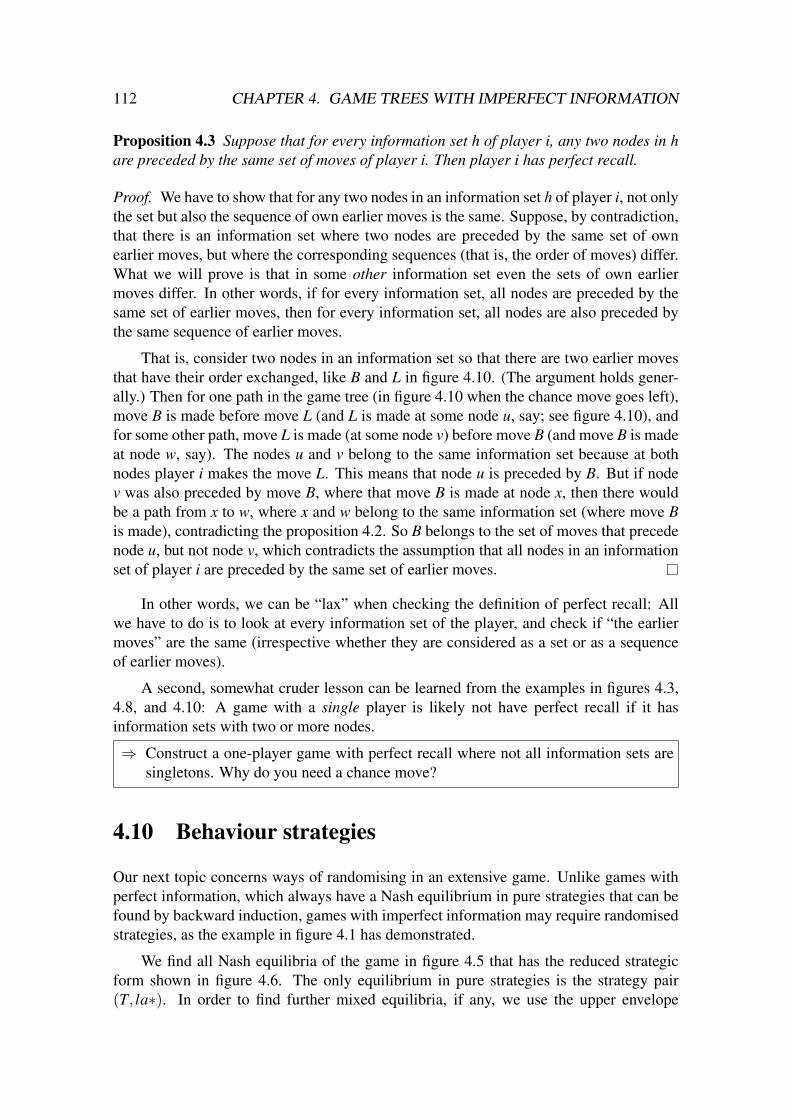
112 CHAPTER 4. GAME TREES WITH IMPERFECT INFORMATION
Proposition 4.3 Suppose that for every information set h of player i, any two nodes in hare preceded by the same set of moves of player i. Then player i has perfect recall.
Proof. We have to show that for any two nodes in an information set h of player i, not onlythe set but also the sequence of own earlier moves is the same. Suppose, by contradiction,that there is an information set where two nodes are preceded by the same set of ownearlier moves, but where the corresponding sequences (that is, the order of moves) differ.What we will prove is that in some other information set even the sets of own earliermoves differ. In other words, if for every information set, all nodes are preceded by thesame set of earlier moves, then for every information set, all nodes are also preceded bythe same sequence of earlier moves.
That is, consider two nodes in an information set so that there are two earlier movesthat have their order exchanged, like B and L in figure 4.10. (The argument holds gener-ally.) Then for one path in the game tree (in figure 4.10 when the chance move goes left),move B is made before move L (and L is made at some node u, say; see figure 4.10), andfor some other path, move L is made (at some node v) before move B (and move B is madeat node w, say). The nodes u and v belong to the same information set because at bothnodes player i makes the move L. This means that node u is preceded by B. But if nodev was also preceded by move B, where that move B is made at node x, then there wouldbe a path from x to w, where x and w belong to the same information set (where move Bis made), contradicting the proposition 4.2. So B belongs to the set of moves that precedenode u, but not node v, which contradicts the assumption that all nodes in an informationset of player i are preceded by the same set of earlier moves.
In other words, we can be “lax” when checking the definition of perfect recall: Allwe have to do is to look at every information set of the player, and check if “the earliermoves” are the same (irrespective whether they are considered as a set or as a sequenceof earlier moves).
A second, somewhat cruder lesson can be learned from the examples in figures 4.3,4.8, and 4.10: A game with a single player is likely not have perfect recall if it hasinformation sets with two or more nodes.
⇒ Construct a one-player game with perfect recall where not all information sets aresingletons. Why do you need a chance move?
4.10 Behaviour strategies
Our next topic concerns ways of randomising in an extensive game. Unlike games withperfect information, which always have a Nash equilibrium in pure strategies that can befound by backward induction, games with imperfect information may require randomisedstrategies, as the example in figure 4.1 has demonstrated.
We find all Nash equilibria of the game in figure 4.5 that has the reduced strategicform shown in figure 4.6. The only equilibrium in pure strategies is the strategy pair(T, la∗). In order to find further mixed equilibria, if any, we use the upper envelope

4.10. BEHAVIOUR STRATEGIES 113
prob(B)
0 11/2 3/4
payoff to II
3
4
5
2
1
0
la*
lb* r*c
r*d
Figure 4.11 Upper envelope of expected payoffs to player II for the game in figure 4.6.
method. Figure 4.11 shows the expected payoffs to player II as a function of the proba-bility that player I chooses B. As this figure shows, the only pairs of strategies betweenwhich player II can be indifferent are la∗ and lb∗ when prob(B) = 1/3; or lb∗ and r∗cwhen prob(B) = 1/2; or r∗c and r∗d when prob(B) = 3/4. The first of these cannot beplayed in an equilibrium because against both la∗ and lb∗, the best response of player Iis T , so that player I cannot be made indifferent between T and B, which is necessary forplayer I wanting to mix between T and B in equilibrium. In the other two cases, how-ever, the pure best responses of player I differ, and it is possible to obtain Nash equilibria.These equilibria are ((1/2,1/2),(0,2/5,3/5,0)) and ((1/4,3/4),(0,0,1/3,2/3)).
What do these mixed strategies mean in terms of the extensive game? For player I,the mixed strategy (1/2,1/2) means that he chooses T and B with equal probability. Forplayer II, the mixed strategy (0,2/5,3/5,0) amounts to choosing lb∗ with probability2/5, and r∗c with probability 3/5. The interpretation of such a mixed strategy is that eachplayer chooses at the beginning of the game a reduced pure strategy, which is a plan ofaction of what do at each reachable information set. The player then sticks to this planof action throughout the game. In particular, if player II has chosen to play lb∗, she firstmakes the move l with certainty, and then move b at her second information set h′. Herreduced pure strategy r∗c is a similar plan of action.
There is a different way of playing such a mixed strategy, which is called a behaviourstrategy. A behaviour strategy is a randomised choice of a move for each information set.That is, rather than using a lottery to determine a (reduced) pure strategy at the begin-ning of the game, the player uses a “local” lottery whenever she reaches an informationset. In our example, player II’s mixed strategy (0,2/5,3/5,0) is then played as follows:At her first information set h, she plays moves l and r with probabilities 2/5 and 3/5,respectively. When she reaches her information set h′ (which is only possible when shehas made the earlier move l), she chooses move a with probability zero and move b withprobability one; this “behaviour” at h′ is deterministic. Similarly, when she reaches herinformation set h′′ (having made move r earlier), then she chooses move c with certainty.

114 CHAPTER 4. GAME TREES WITH IMPERFECT INFORMATION
Definition 4.4 In an extensive game, a behaviour strategy β of player i is defined by aprobability distribution on the set of moves Ch for each information set h of player i. It isgiven by a probability β (c) for each c ∈Ch, that is, a number β (c)≥ 0 for each c ∈Ch sothat ∑c∈Ch
β (c) = 1. In a reduced behaviour strategy, these numbers are left unspecified ifh is unreachable because all earlier own moves by player i that allow her to reach h haveprobability zero under β .
The concept of a reduced behaviour strategy is illustrated by the other mixed equilib-rium of the game in figure 4.5, with the mixed strategy (0,0,1/3,2/3) of player II. Thisis a randomisation between the two pure strategies r∗c and r∗d. It can also be played asa (reduced) behaviour strategy. Namely, at her first information set h, player II choosesl and r with probability 0 and 1, respectively. Then the information set h′ is unreachablebecause it is only reachable when player II makes move l earlier; this event has probabilityzero. Consequently, the behaviour probabilities for making moves a and b are not spec-ified, as in a reduced behaviour strategy. (To obtain an “unreduced” behaviour strategy,one would specify arbitrary probabilities for a and b.) At her information set h′′, player IIchooses c and d with probability 1/3 and 2/3, respectively.
A behaviour strategy can be played by “delaying” the player’s random choice untilshe has reached an information set, when she makes the next move. However, nothingprevents the player making these random choices in advance for each information set,which will then give her a pure strategy that she plays throughout the game. Then thebehaviour strategy is used like a mixed strategy. In other words, behaviour strategies canbe considered as special mixed strategies.
A behaviour strategy β of player i defines a mixed strategy µ in the following way:What we need is the probability µ(π) for a particular pure strategy π in Σi; recall from(4.2) that Σi is the set of pure strategies of player i. This pure strategy π defines a moveπ(h) for each information set h ∈ Hi. When player i uses the behaviour strategy β , thatmove has a certain probability β (π(h)). Because these random moves at the informationsets h of player i are made independently, the probability that all the moves specified byπ are made is the product of these probabilities. That is, the mixed strategy probability is
µ(π) = ∏h∈Hi
β (π(h)). (4.3)
We have been using equation (4.3) when considering a mixed strategy, for exam-ple µ = (0,0,1/3,2/3) in figure 4.5, as a behaviour strategy. That behaviour strategy βwas given by β (l) = 0, β (r) = 1, β (c) = 1/3, and β (d) = 2/3, so that 2/3 = µ(r∗d) =β (r) ·β (∗) ·β (d). This is expressed as a product of three behaviour probabilities, one foreach information set, because the pure strategies are given by a move for each informationset; note that in (4.3), the product has to be taken over all information sets h of player i.There is one complication here, because we are already considering reduced behaviourstrategies and reduced pure strategies: What is meant by β (∗)? This means the behaviourprobability for making any move at h′ (in this case, as part of the pure strategy r∗d),which is unspecified. Clearly, that probability is equal to 1. So we take β (∗) = 1 when-ever applying (4.3) to reduced strategies. Equivalently, we may just omit the unspecifiedbehaviour probabilities from the product, writing simply µ(r∗d) = β (r) ·β (d).

4.10. BEHAVIOUR STRATEGIES 115
The convention β (∗) = 1 is easily seen to agree with the use of (4.3) for unreducedstrategies. For example, consider the unreduced strategic form where r∗d stands for thetwo pure strategies rad and rbd. Each of these has a certain probability under both µ andβ (when extended to the unreduced strategic form), where µ is the representation of β asa mixed strategy. Whatever these probabilities are (obtained by splitting the probabilityfor r∗d into probabilities for rad and rbd), we certainly have
µ(rad)+ µ(rbd) = β (r)β (a)β (d)+β (r)β (b)β (d) = β (r) · (β (a)+β (b)) ·β (d).
The left-hand side is the proper interpretation of the mixed strategy probability µ(r∗d),the right-hand side of β (r) ·β (∗) ·β (d), in agreement with β (∗) = β (a)+β (b) = 1.
•@
@@
@@
¡¡
¡¡
¡
T B
•¢
¢¢
¢¢
AAAAA
a b
•¢
¢¢
¢¢
AAAAA
c d
º
¹
·
¸I
º
¹
·
¸II
º
¹
·
¸II
0 4 1 20 0 0 0
Figure 4.12 Game with four pure strategies of player II. Here, not all mixed strategiesof player II are representable as behaviour strategies.
While every behaviour strategy can be considered as a mixed strategy, the conversedoes not hold. Figure 4.12 shows a game where player II has the four pure strategiesac, ad, bc, bd, which are also her reduced pure strategies. Consider the mixed strategyµ = (1/2,0,0,1/2) of player II, where she chooses the pure strategy ac, that is, moves aand c, with probability 1/2, otherwise the pure strategy bd. Clearly, every move is madewith positive probability overall (in fact, probability 1/2 for each single move). Then if(4.3) was true, then every move combination would have to have positive probability aswell! However, this is not the case, because the strategy ad, for example, has probabilityzero under µ . The reason is that when player II uses µ , the random choice between themoves a and b is correlated with the random choice between c and d. That is, knowingthat move a has been made gives some information about whether move c or d has beenmade (here, the correlation is maximal: move a implies move c). If these random choiceswere made independently, as required in a behaviour strategy, then the random choicebetween a and b would not affect the random choice between c and d.
In this example, the “behaviour” of player II at the left information set in figure 4.12described by µ is to choose a with probability 1/2 and b with probability 1/2, and ditomoves c and d. This defines a behaviour strategy β of player II. This behaviour strategydefines the mixed strategy (1/4,1/4,1/4,1/4) because it chooses each pure strategy withequal probability. This mixed strategy is clearly different from µ .
A second example using figure 4.12 is the mixed strategy µ ′ = (1/6,1/3,1/4,1/4).The corresponding behaviour strategy β ′ has move probabilities β ′(a) = β ′(b) = 1/2,

116 CHAPTER 4. GAME TREES WITH IMPERFECT INFORMATION
because β ′(a) = µ ′(ac) + µ ′(ad) = 1/6 + 1/3, and β ′(c) = µ ′(ac) + µ ′(bc) = 1/6 +1/4 = 5/12 and β ′(d) = µ ′(ad) + µ ′(bd) = 1/3 + 1/4 = 7/12. Again, making thesemoves independently with β ′ results in different probabilities for the pure strategies, forexample in β ′(a) ·β ′(c) = 5/24 for ac, which is different from µ ′(ac).
What we have done in this example is to take a mixed strategy µ of a player and“observe” at each information set of that player the “behaviour” resulting from µ . Thisbehaviour defines a certain behaviour strategy β . In a similar way, β ′ is obtained fromµ ′. The behaviour strategy may differ from the original mixed strategy because with thebehaviour strategy, random choices at different information sets are no longer correlated.However, what does not change are the probabilities of reaching the nodes of game tree,given some (pure or mixed) strategy of the other players. We say that the strategies µand β are equivalent (similarly, µ ′ and β ′ are equivalent). This equivalence holds in anyextensive game with perfect recall. This is the topic of the next section.
⇒ You should now attempt exercise 4.3 on page 123.
4.11 Kuhn’s theorem: behaviour strategies suffice
Information sets were introduced by Harold Kuhn in 1953. His article also defined per-fect recall and behaviour strategies, and proved an important connection between the twoconcepts. This connection is the central property of extensive games and is often called“Kuhn’s theorem”. It says that a player who has perfect recall can always replace a mixedstrategy by an equivalent behaviour strategy.
Why should we even care about whether a player can use a behaviour instead of amixed strategy? The reason is that a behaviour strategy is much simpler to describe thana mixed strategy, significantly so for larger games. As an example, consider a simplifiedpoker game where each player is dealt only a single card, with 13 different possibilitiesfor the rank of that card. A game tree for that game may start with a chance move with13 possibilities for the card dealt to player I, who learns the rank of his card and canthen either “fold” or “raise”. Irrespective of the rest of the game, this defines already213 = 8192 move combinations for player I. Assuming these are all the pure strategiesof player I, a mixed strategy for player I would have to specify 8191 probabilities (whichdetermine the remaining probability because these probabilities sum to one). In contrast, abehaviour strategy would specify one probability (of folding, say) for each possible card,which are 13 different numbers. So a behaviour strategy is much less complex to describethan a mixed strategy.
This example also gives an intuition why a behaviour strategy suffices. The movesat the different decision nodes of player I can be randomised independently because theyconcern disjoint parts of the game. There is no need to correlate the moves for differentcards because in any one game, only one card is drawn.
In general, a player may make moves in sequence and a priori there may be somegain in correlating an earlier move with a subsequent move. This is where the conditionof perfect recall comes in. Namely, the knowledge about any earlier move is already

4.11. KUHN’S THEOREM: BEHAVIOUR STRATEGIES SUFFICE 117
captured by the information sets because perfect recall says that the player knows all hisearlier moves. So there is no need to “condition” a later move on an earlier move becauseall earlier moves are known.
For illustration, consider the game in figure 4.7 which does not have perfect recall.It is easily seen that this game has the same strategic form, shown in figure 4.6, as thegame in figure 4.5, except that the pure strategies of player II are la, lb, ra, rb insteadof the reduced strategies la∗, lb∗, r∗c, r∗d. Here, the mixed strategy (0,2/5,3/5,0) ofplayer II, which selects the pure strategy lb with probability 2/5, and ra with probability3/5, cannot be expressed as a behaviour strategy. Namely, this behaviour strategy wouldhave to choose moves l and r with probability 2/5 and 3/5, respectively, but the probabil-ities for moves a and b, which would be 3/5 and 2/5, are not independent of the earliermove (because otherwise the pure strategy la, for example, would not have probabilityzero). So this mixed strategy, which is part of a Nash equilibrium, cannot be expressed asa behaviour strategy. Using a mixed strategy gives player II more possibilities of playingin the game.
In contrast, the mixed strategy (0,2/5,3/5,0) of player II in the perfect-recall gamein figure 4.5 chooses lb∗ and r∗c with probability 2/5 and 3/5, respectively. As shownearlier, this is in effect a behaviour strategy, because correlating move l with move b, andmove r with move c, is done via the information sets h′ and h′′, which are separate infigure 4.5 but merged in figure 4.7. That is, player II knows that she made move l whenshe has to make her move b at h′, and she knows that she made move r when she has tomake her move c at h′′.
Before stating Kuhn’s theorem, we have to define what it means to say that tworandomised strategies µ and ρ of a player are equivalent. This is the case if for anyfixed strategies of the other players, every node of the game tree is reached with the sameprobability when the player uses µ as when he uses ρ . (Sometimes µ and ρ are alsocalled “realisation equivalent” in this case because every node in the game tree has thesame “realisation probability” when the player uses µ as when he uses ρ .) Two equivalentstrategies µ and ρ always give every player the same expected payoff because the leavesof the game tree are reached with the same probability no matter whether µ or ρ is used.
When are two strategies µ and ρ equivalent? Suppose these are strategies of player i.Consider a particular node, say u, of the game tree. Equivalence of µ and ρ means that,given that the other players play in a certain way, the probability that u is reached is thesame when player i uses µ as when he uses ρ . In order to reach u, the play of the gamehas to make a certain sequence of moves, including chance moves, that lead to u. Thismove sequence is unique because we have a tree. In that sequence, some moves are madeby chance or by players other than player i. These moves have certain given probabilitiesbecause the chance move probabilities and the strategies adopted by the other playersare fixed. We can assume that the overall probability for these moves is not zero, byconsidering fixed strategies of the other players which allow to reach u (otherwise u istrivially reached with the same zero probability with µ as with ρ). So what matters inorder to compare µ and ρ are the moves by player i on the path to u. If the probability forplaying the sequence of moves of player i on the path to u is the same under µ and ρ , and

118 CHAPTER 4. GAME TREES WITH IMPERFECT INFORMATION
if this holds for every node u, then µ and ρ are equivalent. This is the key ingredient ofthe proof of Kuhn’s theorem.
Theorem 4.5 (Kuhn [1953]) If player i in an extensive game has perfect recall, then forany mixed strategy µ of player i there is an equivalent behaviour strategy β of player i.
Proof. We illustrate the proof with the extensive game in figure 4.13, with player II asplayer i. The payoffs are omitted; they are not relevant because only the probabilities ofreaching the nodes of the game tree matter.
II
IIl r
RL
II
d
b
vuh
w
I
c d c
a b a
Figure 4.13 Game illustrating sequences of moves of player II. Payoffs are omitted.
Given µ , we want to construct an equivalent behaviour strategy β . Essentially, theprobability β (c) for any move c at an information set h of player i will be the “observed”probability that player i makes move c when she uses µ . In order to obtain this probability,we consider sequences of moves of player i. Such a sequence is obtained by consideringany node x of the game tree and taking the moves of player i on the path from the rootto x; the resulting sequence shall be denoted by σ i(x). For example, if x is the leaf w ofthe game tree in figure 4.13 and i = II, then that sequence is σ II(w) = lbc, that is, movel followed by b followed by c. If all players are considered, then node w is reached bythe sequence of moves lLbc which includes move L of player I, but that move is ignoredin the definition of σ II(w); for player I, the sequence of moves defined by w is just themove L, that is, σ I(w) = L.
According to definition 4.1, the condition of perfect recall states that the sequence ofown earlier moves is the same for all nodes in an information set. That is,
h ∈ Hi =⇒ ∀u,v ∈ h σ i(u) = σ i(v).
An example is given in figure 4.13 by the information set h where player II has the twomoves c and d, which has two nodes u and v with σ i(u) = σ i(v) = lb. Consequently,

4.11. KUHN’S THEOREM: BEHAVIOUR STRATEGIES SUFFICE 119
the sequence of moves leading to h can be defined uniquely as σh = σ i(u) for any u ∈ h,where i is identified as the player who moves at h, that is, h ∈ Hi. Furthermore, we canextend the sequence σh that leads to h by any move c at h, which we write as the longersequence σhc, to be read as “σh followed by c”. In the example, we have σh = lb, and itcan be extended either by move c or by move d, giving the longer sequences lbc and lbd.Any sequence of moves of player i is either the empty sequence /0 (for example σ i(r) = /0if r is the root of the tree), or it has a last move c made at some information set h ofplayer i, and then it can be written as σhc. So these sequences σhc for h ∈ Hi, c ∈Ch and/0 are all possible sequences of moves of player i.
We now consider the probability µ[σ ] that such a sequence σ of player i is playedwhen player i uses µ . This probability µ [σ ] is simply the combined probability under µfor all the pure strategies that agree with σ in the sense that they prescribe all the movesin σ . For example, if σ = lb in figure 4.13, then the pure strategies of player i that agreewith σ are the strategies that prescribe the moves l and b, which are the pure strategieslbc and lbd. So
µ[lb] = µ(lbc)+ µ(lbd), (4.4)
where µ(lbc) and µ(lbd) are the mixed strategy probabilities for the pure strategies lbcand lbd.
The longer the sequence σ is, the smaller is the set of pure strategies that agree withσ . Conversely, shorter sequences have more strategies that agree with them. The extremecase is the empty sequence /0, because every pure strategy agrees with that sequence.Consequently, we have
µ[ /0] = 1. (4.5)
We now look at a different interpretation of equation (4.4). In this special example,lbc and lbd are also sequences of moves, namely lbc = σhc and lbd = σhd with σh = lb.So the combined probability µ[lbc] of all pure strategies that agree with lbc is simply themixed strategy probability µ(lbc), and similarly µ[lbd] = µ(lbd). Clearly,
µ [lb] = µ[lbc]+ µ [lbd].
In general, considering any information set h of player i, we have the following importantequation:
µ [σh] = ∑c∈Ch
µ[σhc]. (4.6)
This equation holds because because the sequence σh that leads to h is extended by somemove c at h, giving the longer sequence σhc. When considering the pure strategies thatagree with these extended sequences, we obtain exactly the pure strategies that agree withσh.
We are now in a position to define the behaviour strategy β that is equivalent to µ .Namely, given an information set h of player i so that µ [σh] > 0, let
β (c) =µ[σhc]µ[σh]
. (4.7)

120 CHAPTER 4. GAME TREES WITH IMPERFECT INFORMATION
Because of (4.6), this defines a probability distribution on the set Ch of moves at h, asrequired by a behaviour strategy. In (4.7), the condition of perfect recall is used becauseotherwise the sequence σh that leads to the information set h would not be uniquely de-fined.
What about the case µ [σh] = 0? This means that no pure strategy that agrees with σhhas positive probability under µ . In other words, h is unreachable when player i uses µ .We will show soon that µ[σ ] = β [σ ] for all sequences σ of player i. Hence, h is alsounreachable when the player uses β , so that β (c) for c ∈Ch does not need to be defined,that is, β is a reduced behaviour strategy according to definition 4.4. Alternatively, wecan define some behaviour at h (although it will never matter because player i will notmove so as to reach h) in an arbitrary manner, for example by giving each move c at hequal probability, setting β (c) = 1/|Ch|.
We claim that β , as defined by (4.7), is equivalent to µ . We can define β [σ ] for asequence σ of player i, which is the probability that all the moves in σ are made whenthe player uses β . Clearly, this is simply the product of the probabilities for the moves inσ . That is, if σ = c1c2 · · ·cn, then β [σ ] = β (c1)β (c2) · · ·β (cn). When n = 0, then σ isthe empty sequence /0, in which case we set β [ /0] = 1. So we get by (4.7)
β [c1c2 · · ·cn] = β (c1)β (c2) · · ·β (cn) =µ[c1]µ[ /0]
µ [c1c2]µ[c1]
· · · µ[c1c2 · · ·cn−1cn]µ [c1c2 · · ·cn−1]
= µ[c1c2 · · ·cn]
because all the intermediate terms cancel out, and by (4.5). (This is best understood byconsidering an example like σ = lbc = c1c2c3 in figure 4.13.) Because β [σ ] = µ[σ ] forall sequences σ of player i, the strategies β and µ are equivalent, as explained beforetheorem 4.5. The reason is that any node u of the game tree is reached by a uniquesequence of moves of all players and of chance. The moves of the other players havefixed probabilities, so all that matters is the sequence σ i(u) of moves of player i, whichis some sequence σ , which has the same probability no matter whether player i uses β orµ .
4.12 Subgames and subgame perfect equilibria
In an extensive game with perfect information, a subgame is any subtree of the game,given by a node of the tree as the root of the subtree and all its descendants. This definitionhas to be refined when considering games with imperfect information, where every playerhas to know that they have entered the subtree.
Definition 4.6 In an extensive game, a subgame is any subtree of the game tree so thatevery information set is either disjoint to or a subset of the nodes in the subtree.
In other words, if any information set h contains some node of the subtree, then hmust be completely contained in the subtree. This means that the player to move at hknows that he or she is in the subgame. Information sets that have no nodes in the subtreedo not matter.

4.12. SUBGAMES AND SUBGAME PERFECT EQUILIBRIA 121
•@
@@
@@
¡¡
¡¡
¡
º
¹
·
¸II
l rº
¹
·
¸I•
@@
@@
@
¡¡
¡¡
¡
T B
•¢
¢¢
¢¢
AAAAA
a b
•¢
¢¢
¢¢
AAAAA
a b
º
¹
·
¸II
1 3 3 1
3
6 5 0 2
3
@@I
II
T
B
la lb r∗
1 3 3
6 5 3
3 1 3
0 2 3
Figure 4.14 Extensive game and its reduced strategic form. Only one Nash equilibriumof the game is subgame perfect.
In figure 4.14, the subtree with player I’s decision node as root defines a subgame ofthe game. On the other hand, any of the two nodes in player II’s second information setare not roots of subgames, because this information set is neither contained in nor disjointto the respective subtree.
A trivial subgame is either the game itself, or any leaf of the game tree. Some gameshave no other subgames, for example the games in figure 4.1 or 4.5.
⇒ Test your understanding of subgames with exercise 4.4 on page 123.
If every player has perfect recall, then any mixed strategy can be replaced by anequivalent behaviour strategy by Kuhn’s theorem 4.5. The strategies in any Nash equilib-rium can therefore be assumed to be behaviour strategies. A behaviour strategy can easilybe restricted to a subgame, by ignoring the behaviour probabilities for the informationsets that are disjoint to the subgame.
Definition 4.7 In an extensive game with perfect recall, a subgame perfect Nash equilib-rium (SPNE) is a profile of behaviour strategies that defines a Nash equilibrium for everysubgame of the game.
In figure 4.14, the reduced strategic form of the extensive game is shown on theright. If one ignores the third strategy r∗ of player II in this strategic form, the resulting2× 2 game, with columns called a and b instead of la and lb, defines the strategic formof the subgame that starts with the move of player I. This subgame has a unique mixedequilibrium, where player I chooses T,B with probabilities 2/3,1/3, and player II choosesa,b with probabilities 1/2,1/2. The resulting payoffs to player I and II are 2 and 4, whichcan be substituted for the subgame to obtain a smaller game where player II choosesbetween l and r. Then it is optimal for player II to choose l with certainty. This defines abehaviour strategy for each player, which is an SPNE.

122 CHAPTER 4. GAME TREES WITH IMPERFECT INFORMATION
The step of computing an equilibrium of a subgame and substituting the resultingequilibrium payoffs for the subgame generalises the backward induction step in gameswith perfect information. In games with perfect information, this backward inductionstep amounts to finding an optimal move of a single player in a very simple subgamewhere each move leads directly to a payoff. The optimal move defines an equilibrium inthat subgame. In a game with imperfect information, the subgame may involve more thanone player, and the equilibrium is usually more difficult to find.
The described SPNE of the extensive game in figure 4.12 is the mixed-strategy equi-librium ((2/3,1/3),(1/2,1/2,0)) of the reduced strategic form, which also defines a pairof behaviour strategies. Another Nash equilibrium is the pair (B,r∗) of reduced purestrategies. The strategy r∗ is only a reduced behaviour strategy for player II, because itdoes not specify the probabilities for the moves a and b at her second information set(which is unreachable when she makes move r). However, no matter how the behaviourprobabilities for player II’s moves a and b are specified, they are not part of a Nash equi-librium of the subgame when player I makes move B. Consequently, we can safely saythat (B,r∗) does not correspond to an SPNE of the game.
In general, just as for games with perfect information, an equilibrium of an extensivegame can only be called subgame perfect if each player’s behaviour (or pure) strategy isnot reduced, but is fully specified and defines a probability distribution (or deterministicmove) for each information set of the player.
We described for the example in figure 4.14 how to find an SPNE, which generalisesthe backward induction process. Starting with each leaf of the game tree (which repre-sents a trivial subgame), one considers any subgame that does not have any non-trivialsubgames on its own. This subgame has an equilibrium by Nash’s theorem. The mixedstrategies in this equilibrium can be represented as behaviour strategies by Kuhn’s theo-rem. The resulting expected payoffs to the players in the equilibrium are then assigned toa new leaf that substitutes the considered subgame, and then this is iterated. (Unlike ingames with perfect information, however, the step of finding an equilibrium of a subgamemay involve a large game, for example if the game has no non-trivial subgames at all,where the next subgame considered after each leaf is the entire game.) This construc-tion gives an SPNE; we omit the proof that we obtain indeed an equilibrium of the entiregame, which is analogous to the theorem that asserts that backward induction defines anequilibrium. We summarise the existence of SPNE in the last theorem of this chapter.
Theorem 4.8 Any extensive game with perfect recall has an SPNE in behaviour strate-gies.
4.13 Exercises for chapter 4
Exercise 4.1 shows how, with the help of information sets, any strategic-form game(where the players move simultaneously) can be represented as an extensive game. Exer-cise 4.2 asks to look at a number of extensive games, to check whether they have perfectrecall, and to find all their equilibria using the methods from earlier chapters. Exercise 4.4

4.13. EXERCISES FOR CHAPTER 4 123
shows that information sets can intersect a path in the game tree only once, and tests yourunderstanding of the concept of subgames. In exercise 4.3, you have to construct an ex-tensive game with imperfect information, which tests your understanding of informationsets; for the analysis of this game, the theory of zero-sum games is useful.
Exercise 4.1 Explain two ways, with either player I or player II moving first, of rep-resenting an m× n bimatrix game as an extensive game that has the given game as itsstrategic form. Giving an example may be helpful. In each case, what are the number ofdecision nodes of player I and of player II, respectively? How many terminal nodes doesthe game tree have? Why do we need information sets here?
Exercise 4.2 Which of the six pictures in figure 4.15 define extensive games where eachplayer has perfect recall, and which do not? The games (a) and (b) are zero-sum games,with payoffs to player I. For each of the “legal” extensive games with perfect recall, findall Nash equilibria in pure or mixed strategies. Justify your answers.
Exercise 4.3 Consider the following two-person zero-sum game: A deck has three cards(of different ranks: High, Middle, Low), and each player is dealt a card. All deals areequally likely, and of course the players get different cards. A player does not know thecard dealt to the other player. After seeing his hand, player I has the option to Raise (R) orFold (F). When he folds, he loses one unit to the other player. When he raises, player IIhas the option to meet (m) or pass (p). When player II chooses “pass”, he will have to payplayer I one unit. When player II chooses “meet”, the higher card wins, and the playerwith the lower card has to pay two units to the winning player.
(a) Draw a game in extensive form that models this game, with information sets, andpayoffs to player I at the leaves.
(b) Simplify this game by assuming that at an information set where a player’s move isalways at least as good as the other move, no matter what the other player’s move orthe chance move were or will be, then the player will choose that move. Draw thesimplified extensive form game.
(c) What does the simplification in (b) have to do with weakly dominated strategies?Why is the simplification legitimate here?
(d) Give the strategic form of the simplified game from (b) and find an equilibrium ofthat game. What are the behaviour probabilities of the players in that equilibrium?What is the unique payoff to the players in equilibrium?
Exercise 4.4 For an extensive game with perfect recall, show that the the information setcontaining the root (starting node) of any subgame is always a singleton (that is, containsonly that node).[Hint: Use proposition 4.2 on page 110.]

124 CHAPTER 4. GAME TREES WITH IMPERFECT INFORMATION
(a)
(c)
(e)
(b)
(d)
(f)
����
����
����
����
����
I
RL
II
I
II
a ab b
5 1 4
2 3
1
c d
S T
����
����
����
����
����
I
II
II
I
RL
S
a ab b
c d
T
5 1 4
2 3
1
����
����
����
����
I
II
II
a ab b
T B
l r
22
00
1 13 3
13
����
���� I
II
a b
T B
22
00
11
����
����
����
����
I
II
II
RL
c
a ab b
d
30
5 2 6 00 0 21
����
����
����
����
I
II
I
RL
S
a ab b
T
30
5 2 6 00 0 21
Figure 4.15 Extensive games for exercise 4.2.

Chapter 5
Bargaining
This chapter presents models of bargaining. Chapter 2 has to be understood first, as wellas the concept of max-min strategies from section 3.14.
5.1 Learning objectives
After studying this chapter, you should be able to:• explain the concepts of bargaining sets, bargaining axioms, Nash bargaining solution,
threat point, and Nash product;• draw bargaining sets derived from bimatrix games, and for bargaining over a “unit
pie” when players have concave utility functions;• explain, and solve specific examples of, the model of bargaining over multiple rounds
of demands and counter-demands, and of stationary SPNE for infinitely many rounds.
5.2 Further reading
Chapters 15 and 7 of• Osborne, Martin J., and Ariel Rubinstein A Course in Game Theory. (MIT Press,
1994) [ISBN 0262650401].The original article on the iterated-offers bargaining model is
• Rubinstein, Ariel “Perfect equilibrium in a bargaining model.” Econometrica, Vol. 50(1982), pp. 97–109.
5.3 Introduction
This chapter treats bargaining situations. This is a very practical game-theoretic problemthat, for example, buyers and sellers encounter in real life. The two players have some-thing to gain by reaching an agreement. This approach belongs to “cooperative gametheory”, which tries to guide players that have decided to cooperate.
125

126 CHAPTER 5. BARGAINING
A basic bargaining model is that of “splitting a pie” in a way that is acceptable to bothplayers, but where within that range a player can only gain at the expense of the other. Thequestion is how to split the pie fairly. In his undergraduate thesis, John Nash proposed asystem of “axioms”, or natural conditions, that should allow an impartial judge to arriveat a fair “bargaining solution”. Nash showed that these axioms always entail a uniquesolution, which is also easy to calculate. Nash’s development is presented in sections 5.4to 5.6.
The later sections of this chapter go back to the game-theoretic models consideredearlier which, unlike the Nash bargaining solution, are “non-cooperative” in nature, mean-ing that players have no recourse to a judge but have to follow their own incentives asmodelled with actions and payoffs in the game. Here, bargaining is modelled by playersalternately making offers which the other player can accept or reject. The analysis of thisgame uses the study of commitment games learned at the end of Chapter 2. The most ba-sic form is the “ultimatum game” that consists of a single take-it-or-leave-it offer whichcan only be accepted or rejected.
With alternating offers over several rounds, there is a chance at each stage that thegame does not proceed to the next round so that players wind up with nothing becausethey could not agree. The effect of this is a “discount factor” which quantifies to whatextent an earlier agreement is better that a later one. By thinking ahead, the optimalstrategies of the players define sequences of alternating offers, with agreement in the firstround. This can be done with a fixed number of rounds, or with “stationary strategies” foran infinite number of bargaining rounds where, in essence, the game repeats every tworounds when it comes back to the same player to make an offer.
The nice conclusion of this alternating-offers bargaining model is that when the dis-count factor represents very patient players, it gives the same outcome as Nash’s axiomaticbargaining solution. Nash’s “cooperative” solution concept is thereby given a good foun-dation in terms of self-interested behaviour.
5.4 Bargaining sets
Consider the variant of the prisoner’s dilemma game on the left in figure 5.1. Player I’sstrategy B dominates T , and r dominates l, so that the unique Nash equilibrium of thegame is (B,r) with payoff 1 to both players. The outcome (T, l) would give payoffs 2and 3 to players I and II, which would clearly be better.
Suppose now that the players can talk to each other and have some means of enforcingan agreement, for example by entering some legal contract that would be very costly tobreak. We do not model how the players can talk, agree, or enforce contracts, but insteadtry to give guidelines about the agreement they can reach.
The first step is to model what players can achieve by an agreement, by describing a“bargaining set” of possible payoff pairs that they can bargain over. Suppose that the play-ers can agree to play any of the cells of the payoff table. The resulting utility pairs (u,v)are dots in a two-dimensional diagram with horizontal coordinate u (utility to player I)

5.4. BARGAINING SETS 127
and vertical coordinate v (utility to player II). These dots are shown on the right in fig-ure 5.1, marked with the respective strategy pairs, for example T, l marking the utility pair(2,3).
@@@I
II
T
B
l r
2 0
3 4
5 1
0 1
0 1
1
0
2
2
3
3
4
4 5
T,l
B,rB,l
T,r
S
v
u
( )U,V
Figure 5.1 Left: 2× 2 game similar to the prisoner’s dilemma. Right: correspondingbargaining set S (dark grey), and its bargaining solution (U,V ).
The convex hull (set of convex combinations) of these utility pairs is shown in lightand dark grey in figure 5.1. Any such convex combination is obtained by a joint lotterythat the players have decided to play as a possible result of their agreement. For example,the utility pair (1.5,2) would be the expected utility if the players have decided to toss afair coin, and, depending on the outcome, to either play (T, l) or else (B,r); we assumethat this play is part of the players’ contract that they have to adhere to.
Making the bargaining set convex with the help of lotteries is not as strange as itsounds. For example, if two people find something that both would like to have but thatcannot be divided, tossing a coin to decide who gets it is an accepted fair solution.
Not every point in the convex hull is “reasonable” because we always assume thatthe players have the option not to agree. For example, player I would not agree that bothplayers choose only the strategy pair (T,r), where player I gets payoff zero. The reason isthat without any agreement, player I can use his max-min strategy B that guarantees him apayoff of 1 irrespective of what the other player does. As shown in the earlier section onzero-sum games, a max-min strategy may be a mixed strategy; in the prisoner’s dilemmagame it is a pure strategy, in fact the dominating strategy. We ask that every agreedoutcome of the bargaining situation should give each player at least his or her max-minpayoff (which is, as usual, defined in terms of that player’s own payoffs).
The bargaining set S derived from a two-player game in strategic form is thus definedas the convex hull of utility pairs (as specified in the game), with the additional constraintthat u ≥ u0 and v ≥ v0 for all (u,v) in S, where u0 is the max-min payoff to player I andv0 is the max-min payoff to player II. With u0 = v0 = 1, the resulting set S is shown indarker grey in figure 5.1.
In this example, the “Nash bargaining solution” (which is not to be confused with“Nash equilibrium”, a very different concept) will give the utility pair (U,V ) = (2.5,2.5),

128 CHAPTER 5. BARGAINING
as we will explain (the fact that U = V is a coincidence). This expected payoff pair is aconvex combination of the utility pairs (2,3) and (5,0). It is achieved by a joint lotteryof playing T, l with probability 5/6 and B, l with probability 1/6. In effect, player IIalways plays l and player I randomises between T and B with probabilities 5/6 and 1/6.However, this is not a “mixed strategy” but rather a lottery performed by a third party,with an outcome that both players (in particular player II) have decided to accept.
5.5 Bargaining axioms
We consider bargaining situations modelled as bargaining sets, and try to obtain a “so-lution” for any such situation. The conditions about this model are called axioms andconcern the bargaining set itself, as well as the solution one wants to obtain for any suchset.
Definition 5.1 (Axioms for bargaining set) A bargaining set S with threat point (u0,v0)is a non-empty subset of R2 so that
(a) u≥ u0, v≥ v0 for all (u,v) ∈ S;
(b) S is compact;
(c) S is convex.
Each pair (u,v) in a bargaining set S represents a utility u for player I and a utility vfor player II which the players can achieve by reaching a specific agreement. At leastone agreement is possible because S is non-empty. The threat point (u0,v0) is the pair ofutilities that each player can (in expectation) guarantee for himself or herself. Axiom (b)in definition 5.1 states that S is bounded and closed, so it is possible define a “bargainingsolution” by some sort of maximisation process. The convexity axiom (c) means thatplayers have access to joint lotteries as part of their agreement, if necessary.
In section 5.4, we have constructed a bargaining set S from a bimatrix game, andnow argue that it fulfils the axioms in definition 5.1. This is clear for (b) and (c). Byconstruction, (a) holds, but we have to show that S is not empty. The threat point (u0,v0)is obtained with u0 as the max-min payoff to player I (in terms of his payoffs) and v0as the max-min payoff to player II (in terms of her payoffs). Thus, if player I playshis max-min strategy x and player II plays her max-min strategy y, then the payoff pair(u,v) = (a(x, y),b(x, y)) that results in the game is an element of S because u ≥ u0 andv≥ v0, so S is not empty.
⇒ Try exercise 5.1 on page 152.
However, in the construction of a bargaining set from a bimatrix game, the threatpoint (u0,v0) need not itself be an element of S, as shown in exercise 5.1. For this reason,the threat point (u0,v0) is explicitly stated together with the bargaining set. If the threatpoint belongs to S and (a) holds, then there can be no other threat point. The axioms indefinition 5.2 below would be easier to state if the threat point was included in S, but thenwe would have to take additional steps to obtain such a bargaining set from a bimatrix

5.5. BARGAINING AXIOMS 129
game. In our examples and drawings we will typically consider sets S that include thethreat point.
From now on, we simply assume that the bargaining set S fulfils these axioms. Wewill later consider bargaining sets for other situations, which are specified directly andnot from a bimatrix game.
In the following definition, the axioms (d)–(h) continue (a)–(c) from definition 5.1.We discuss them afterwards.
Definition 5.2 (Axioms for bargaining solution) For a given bargaining set S with threatpoint (u0,v0), a bargaining solution N(S) is a pair (U,V ) so that
(d) (U,V ) ∈ S;
(e) the solution (U,V ) is Pareto-optimal, that is, for all (u,v) ∈ S, if u ≥U and v ≥ V ,then (u,v) = (U,V );
(f) it is invariant under utility scaling, that is, if a,c > 0, b,d ∈R and S′ is the bargainingset {(au + b,cv + d) | (u,v) ∈ S} with threat point (au0 + b,cv0 + d), then N(S′) =(aU +b,cV +d);
(g) it preserves symmetry, that is, if u0 = v0 and if any (u,v) ∈ S fulfils (v,u) ∈ S, thenU = V ;
(h) it is independent of irrelevant alternatives: If S,T are bargaining sets with the samethreat point and S⊂ T , then either N(T ) 6∈ S or N(T ) = N(S).
The notation N(S) is short for “Nash bargaining solution”. The solution is a pair(U,V ) of utilities for the two players that belongs to the bargaining set S by axiom (d).
The Pareto-optimality stated in (e) means that it should not be possible to improvethe solution for one player without hurting the other player. Graphically, the solution istherefore on the upper-right (or “north-east”) border of the bargaining set, which is alsocalled the Pareto-frontier of the set.
Invariance under utility scaling as stated in (f) means the following. The utility func-tion of a player can be changed by changing its “scale” and “base point” without changingits meaning, just like a temperature scale. Such a change for player I means that insteadof u we consider au + b where a and b are fixed real numbers and a > 0. Similarly, forplayer II we can replace v by cv+d for fixed c,d and c > 0. When drawing the bargainingset S, this means that (by adding b) the first coordinate of any point in that set is movedby the amount b (to the right or left depending on whether b is positive or negative), andstretched by the factor a (if a > 1, and shrunk if a < 1). In (f), the set S′ and the new threatpoint are obtained from S by applying such a “change of scale” for both players.
Because this scaling does not change the meaning of the utility values (they stillrepresent the same preference), the bargaining solution should not be affected either, asstated in axiom (f). In a sense, this means the bargaining solution should not dependon a direct comparison of the players’ utilities. For example, if you want to split a barof chocolate with a friend you cannot claim more because you like chocolate “ten timesmore than she does” (which you could represent by changing your utility from u to 10u),
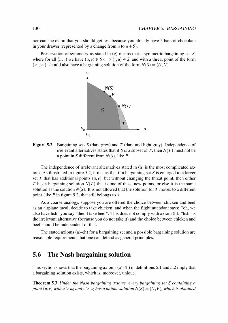
130 CHAPTER 5. BARGAINING
nor can she claim that you should get less because you already have 5 bars of chocolatein your drawer (represented by a change from u to u+5).
Preservation of symmetry as stated in (g) means that a symmetric bargaining set S,where for all (u,v) we have (u,v) ∈ S⇐⇒ (v,u) ∈ S, and with a threat point of the form(u0,u0), should also have a bargaining solution of the form N(S) = (U,U).
v
uvu
0
0
N(T)
N(S)P
S
T
Figure 5.2 Bargaining sets S (dark grey) and T (dark and light grey). Independence ofirrelevant alternatives states that if S is a subset of T , then N(T ) must not bea point in S different from N(S), like P.
The independence of irrelevant alternatives stated in (h) is the most complicated ax-iom. As illustrated in figure 5.2, it means that if a bargaining set S is enlarged to a largerset T that has additional points (u,v), but without changing the threat point, then eitherT has a bargaining solution N(T ) that is one of these new points, or else it is the samesolution as the solution N(S). It is not allowed that the solution for T moves to a differentpoint, like P in figure 5.2, that still belongs to S.
As a coarse analogy, suppose you are offered the choice between chicken and beefas an airplane meal, decide to take chicken, and when the flight attendant says: “oh, wealso have fish” you say “then I take beef”. This does not comply with axiom (h): “fish” isthe irrelevant alternative (because you do not take it) and the choice between chicken andbeef should be independent of that.
The stated axioms (a)–(h) for a bargaining set and a possible bargaining solution arereasonable requirements that one can defend as general principles.
5.6 The Nash bargaining solution
This section shows that the bargaining axioms (a)–(h) in definitions 5.1 and 5.2 imply thata bargaining solution exists, which is, moreover, unique.
Theorem 5.3 Under the Nash bargaining axioms, every bargaining set S containing apoint (u,v) with u > u0 and v > v0 has a unique solution N(S) = (U,V ), which is obtained

5.6. THE NASH BARGAINING SOLUTION 131
as the point (u,v) that maximises the product (also called the “Nash product”) (u−u0)(v− v0) for (u,v) ∈ S.
Proof. First, consider the set S′ = {(u−u0,v− v0) | (u,v) ∈ S}, which is the set S trans-lated so that the threat point (u0,v0) is simply the origin (0,0). Maximising the Nashproduct now amounts to maximising u · v for (u,v) ∈ S. Let (U,V ) be the utility pair(u,v) where this happens, where by assumption UV > 0. We re-scale the utilities so that(U,V ) = (1,1), by replacing S with the set S′′ = {(u/U,v/V ) | (u,v) ∈ S}.
We now consider the set T = {(u,v) | u ≥ 0, v ≥ 0, u + v ≤ 2}. For the bargainingset T , the solution is N(T ) = (1,1), because T is a symmetric set, and (1,1) is the onlysymmetric point on the Pareto-frontier of T . We claim that S⊆ T . Then, by the indepen-dence of irrelevant alternatives, N(S) must be equal to N(T ) because this point (1,1) isan element of S, so because it is not the case that N(T ) 6∈ S, we must have N(S) = N(T ).
Proving S ⊆ T uses the convexity of S. Namely, suppose there was a point (u,v) inS which is not in T . Because u ≥ 0, v ≥ 0, this means u + v > 2. The idea is now thateven if the Nash product u · v is not larger than 1 (which is the Nash product UV ), thenthe Nash product uv of a suitable convex combination (u,v) = (1− ε)(U,V )+ ε(u,v) islarger than 1. Here, ε will be a small positive real number.
uv = 1
u v( , )
u v( , )
v
20u
1
1
2
S
T
(1,1)
Figure 5.3 Proof that the point (u,v), which is outside the triangle T (dark and lightgrey), cannot belong to S (dark grey), which shows that S⊆ T .
This is illustrated in figure 5.3: The hyperbola {(u,v) | uv = 1} touches the set T atthe point (1,1). The tangent to the hyperbola is the line through points (2,0) and (0,2),which is the Pareto-frontier of T . Because the point (u,v) is to the right of that tangent,the line segment that connects (1,1) and (u,v) must intersect the hyperbola and thereforecontain points (u,v) to the right of the hyperbola, where uv > 1. This is a contradiction,because (u,v) ∈ S since S is convex, but the maximum Nash product of a point in S is 1.
So consider the Nash product for the convex combination (u,v) of (1,1) and (u,v):

132 CHAPTER 5. BARGAINING
uv = [(1− ε)U + εu][(1− ε)V + εv]= [U + ε(u−U)][V + ε(v−V )]
= UV + ε[u+ v− (U +V )+ ε(u−U)(v−V )].
Now, because u + v > 2, but U +V = 2, the term u + v− (U +V ) is positive, and ε(u−U)(v−V ) can be made smaller than that term in absolute value, for suitably small ε > 0,even if (u−U)(v−V ) is any negative number. Consequently, uv > 1 =UV for sufficientlysmall positive ε , which shows that UV was not the maximum Nash product in S, whichcontradicts the construction of (U,V ). This proves that, indeed, S⊆ T , and hence N(S) =N(T ) as claimed.
In order to show that the point (U,V ) = (1,1) is unique, we can again look at thehyperbola, and argue similarly as before. Namely, suppose that (u,v) is a point in Sdifferent from (1,1) so that u · v = 1. Then this point and (1,1) are two points on thehyperbola, and points on the line segment joining these two points belong to S because Sis convex. However, they have a larger Nash product. For example, the mid-point 1/2 ·(1,1)+1/2 ·(u,v) has the Nash product (1/2+u/2)(1/2+v/2) = 1/4+u/4+v/4+u ·v.Because u · v = 1, this is equal to 1/2 +(u + v)/4, which is larger than 1 if and only if(u+v)/4 > 1/2 or u+v > 2. The latter condition is equivalent to u+1/u > 2 or, becauseu > 0, to u2 +1 > 2u or u2−2u+1 > 0, that is, (u−1)2 > 0, which is true because u 6= 1.So, again because S is convex, the Nash product has a unique maximum in S.
The assumption that S has a point (u,v) with u > u0 and v > v0 has the followingpurpose: Otherwise, for (u,v) ∈ S, all utilities u of player I or v of player II (or both) fulfilu = u0 or v = v0, respectively. Then the Nash product (U − u0)(V − v0) for (U,V ) ∈ Swould always be zero, so it has no unique maximum. In this rather trivial case, thebargaining set S is either just the singleton {(u0,v0)} or a line segment {u0}× [v0,V ] or[u0,U ]×{v0}. In both cases, the Pareto-frontier consists of a single point (U,V ), whichdefines the unique Nash solution N(S).
⇒ If the bargaining set is a line segment as discussed in the preceding paragraph, whyis its Pareto-frontier a single point? Is this always so if the line segment is notparallel to one of the coordinate axes?
It can be shown relatively easily that the maximisation of the Nash product as de-scribed in theorem 5.3 gives a solution (U,V ) that fulfils the axioms in definitions 5.1and 5.2.
⇒ In exercise 5.2, you are asked to verify this for axiom (f).
We describe how to find the bargaining solution (U,V ) for the bargaining set S infigure 5.1. The threat point (u0,v0) is (1,1). The Pareto-frontier consists of two linesegments, a first line segment joining (1,3.5) to (2,3), and a second line segment joining(2,3) to (4,1). The Nash product (u−u0)(v− v0) for a point (u,v) on the Pareto-frontieris the size of the area of the rectangle between the threat point (u0,v0) and the point (u,v).In this case, the diagram shows that the second line segment creates the larger rectanglein that way. A point on the second line segment is of the form (1− p)(2,3)+ p(4,1) for0≤ p≤ 1, that is, (2+2p,3−2p). Because (u0,v0) = (1,1), the resulting Nash product

5.6. THE NASH BARGAINING SOLUTION 133
is (1 + 2p)(2− 2p) or 2 + 2p− 4p2. The unique maximum over p of this expressionis obtained for p = 1/4 because that is the zero of its derivative 2− 8p, with negativesecond derivative so this is a maximum. The point (U,V ) is therefore given as (2.5,2.5).(In general, such a maximum can result for p < 0 or p > 1, which implies that the leftor right endpoint of the line segment with p = 0 or p = 1, respectively, gives the largestvalue of the Nash product. Then one has to check the adjoining line segment for a possiblylarger Nash product, which may occur on the corner point.)
The following proposition gives a useful condition to find the bargaining solutiongeometrically. It is of particular importance later, in section 5.12.
Proposition 5.4 Suppose that the Pareto-frontier of a bargaining set S with threat point(0,0) is given by {(u, f (u)) | 0≤ u≤ 1} for a decreasing and continuous function f withf (0) = 1 and f (1) = 0. Then the bargaining solution (U,V ) is the unique point (U, f (U))where the bargaining set has a tangent with slope − f (U)/U. If f is differentiable, thenthis slope is the derivative f ′(U) of f at U, that is, f ′(U) =− f (U)/U.
αα
1
v = f u
10u
( )
( )U,V
αα
uv = constant1
v
10u
( )U,V
Figure 5.4 Characterisation of the Nash bargaining solution for differentiable (left) andnon-differentiable bargaining frontier (right).
Proof. We first consider the case that the function f that defines the Pareto-frontier isdifferentiable. The bargaining solution maximises the Nash product u · f (u) on the Pareto-frontier. This requires the derivative with respect to u to be zero, that is, f (u)+u · f ′(u)= 0or f ′(u) = − f (u)/u, so U has to solve this equation as claimed. The solution is alsounique: f ′(u) is negative and decreasing with u because the bargaining set is convex (so fis a concave function, see the definition in (5.1) below); furthermore, the function f (u) isdecreasing and 1/u (where we can assume u > 0) is strictly decreasing, so that − f (u)/uis strictly increasing, and hence there is at most one u with f ′(u) =− f (u)/u.
The left picture in figure 5.4 shows the line connecting the origin (0,0) with (U,V ),which has the slope V/U , that is, f (U)/U , as indicated by the angle α near the origin. Thetangent of the Pareto-frontier at the point (U,V ) slopes downwards, with negative slopef ′(U). The equation f ′(U) = − f (U)/U states that this tangent intersects the horizontal
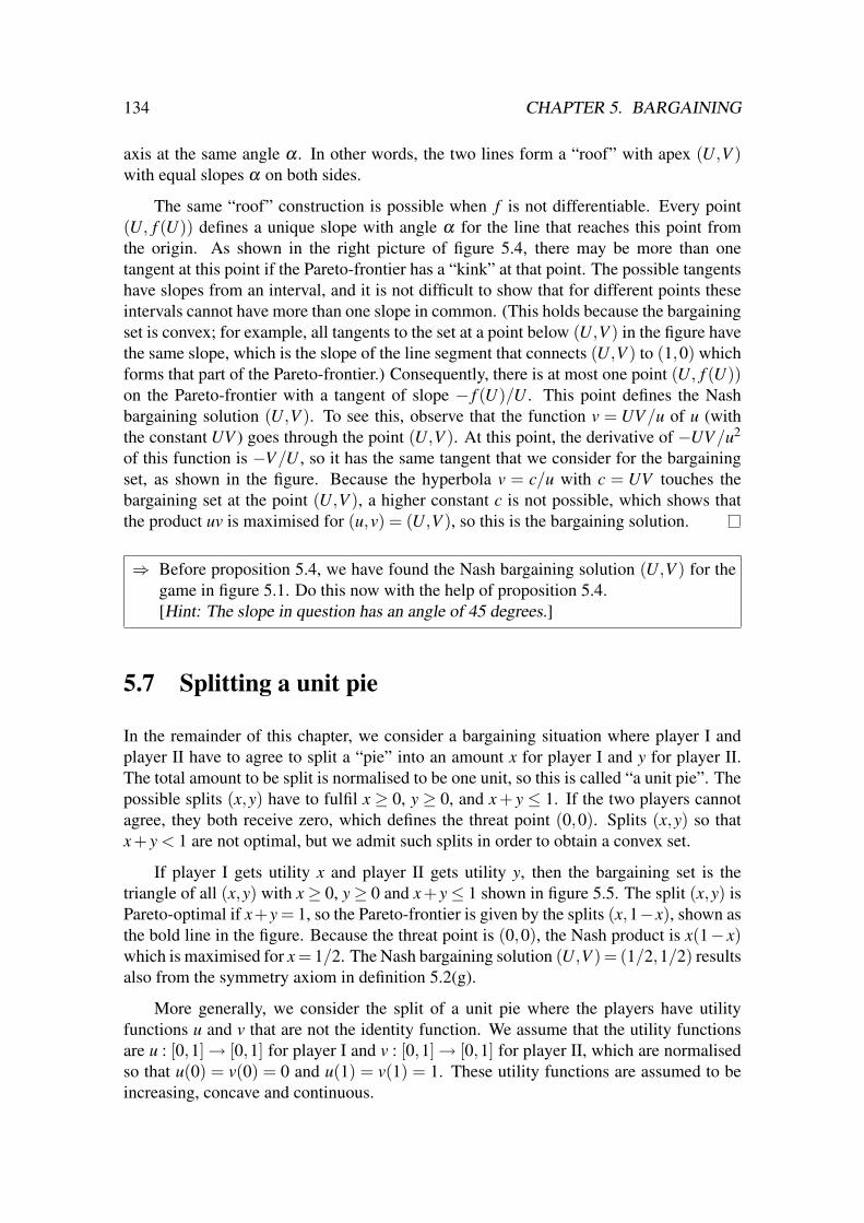
134 CHAPTER 5. BARGAINING
axis at the same angle α . In other words, the two lines form a “roof” with apex (U,V )with equal slopes α on both sides.
The same “roof” construction is possible when f is not differentiable. Every point(U, f (U)) defines a unique slope with angle α for the line that reaches this point fromthe origin. As shown in the right picture of figure 5.4, there may be more than onetangent at this point if the Pareto-frontier has a “kink” at that point. The possible tangentshave slopes from an interval, and it is not difficult to show that for different points theseintervals cannot have more than one slope in common. (This holds because the bargainingset is convex; for example, all tangents to the set at a point below (U,V ) in the figure havethe same slope, which is the slope of the line segment that connects (U,V ) to (1,0) whichforms that part of the Pareto-frontier.) Consequently, there is at most one point (U, f (U))on the Pareto-frontier with a tangent of slope − f (U)/U . This point defines the Nashbargaining solution (U,V ). To see this, observe that the function v = UV/u of u (withthe constant UV ) goes through the point (U,V ). At this point, the derivative of −UV/u2
of this function is −V/U , so it has the same tangent that we consider for the bargainingset, as shown in the figure. Because the hyperbola v = c/u with c = UV touches thebargaining set at the point (U,V ), a higher constant c is not possible, which shows thatthe product uv is maximised for (u,v) = (U,V ), so this is the bargaining solution.
⇒ Before proposition 5.4, we have found the Nash bargaining solution (U,V ) for thegame in figure 5.1. Do this now with the help of proposition 5.4.[Hint: The slope in question has an angle of 45 degrees.]
5.7 Splitting a unit pie
In the remainder of this chapter, we consider a bargaining situation where player I andplayer II have to agree to split a “pie” into an amount x for player I and y for player II.The total amount to be split is normalised to be one unit, so this is called “a unit pie”. Thepossible splits (x,y) have to fulfil x ≥ 0, y ≥ 0, and x + y ≤ 1. If the two players cannotagree, they both receive zero, which defines the threat point (0,0). Splits (x,y) so thatx+ y < 1 are not optimal, but we admit such splits in order to obtain a convex set.
If player I gets utility x and player II gets utility y, then the bargaining set is thetriangle of all (x,y) with x≥ 0, y≥ 0 and x+ y≤ 1 shown in figure 5.5. The split (x,y) isPareto-optimal if x+y = 1, so the Pareto-frontier is given by the splits (x,1−x), shown asthe bold line in the figure. Because the threat point is (0,0), the Nash product is x(1− x)which is maximised for x = 1/2. The Nash bargaining solution (U,V ) = (1/2,1/2) resultsalso from the symmetry axiom in definition 5.2(g).
More generally, we consider the split of a unit pie where the players have utilityfunctions u and v that are not the identity function. We assume that the utility functionsare u : [0,1]→ [0,1] for player I and v : [0,1]→ [0,1] for player II, which are normalisedso that u(0) = v(0) = 0 and u(1) = v(1) = 1. These utility functions are assumed to beincreasing, concave and continuous.
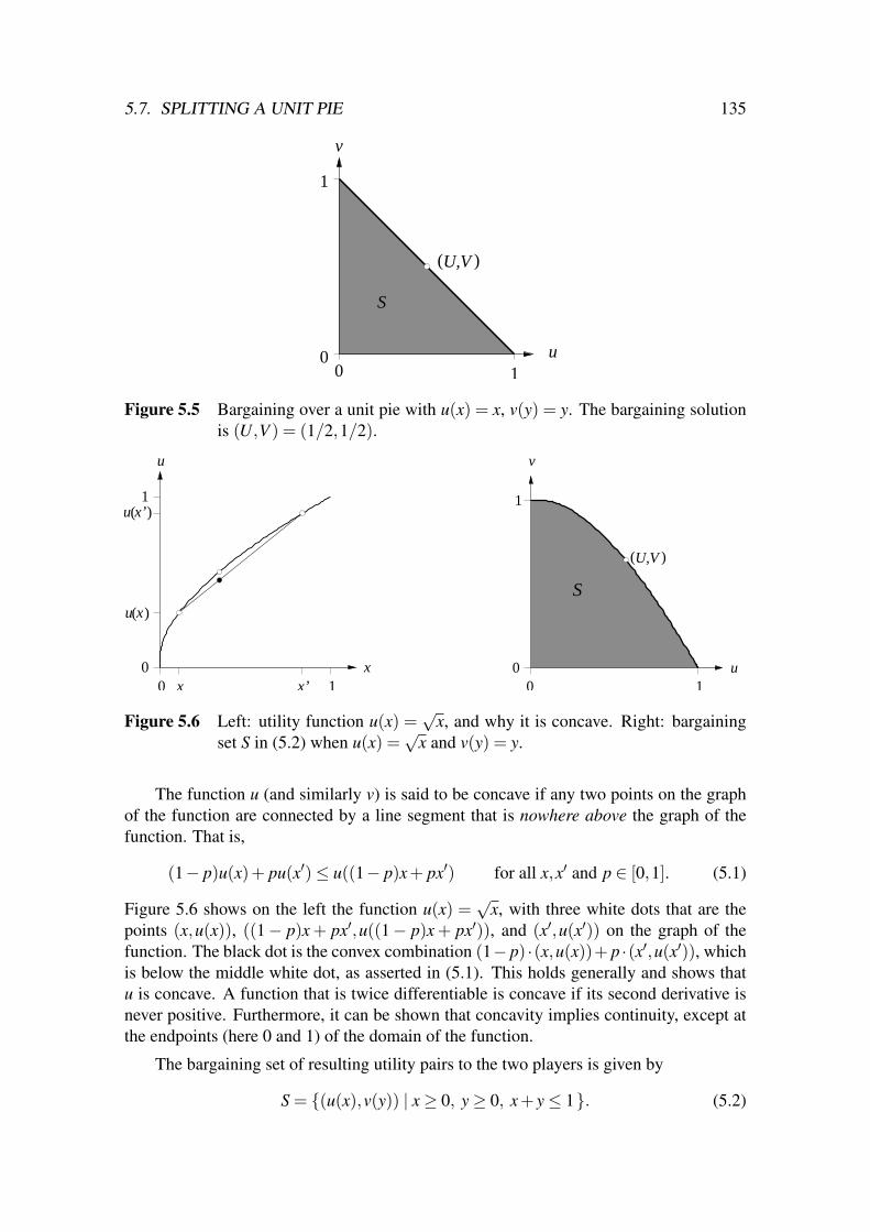
5.7. SPLITTING A UNIT PIE 135
v
u
1
00 1
S
( )U,V
Figure 5.5 Bargaining over a unit pie with u(x) = x, v(y) = y. The bargaining solutionis (U,V ) = (1/2,1/2).
u
u x
u x’
x 1
0
1
x x’0
( )
( )
u
v
0
1
0 1
( )U,V
S
Figure 5.6 Left: utility function u(x) =√
x, and why it is concave. Right: bargainingset S in (5.2) when u(x) =
√x and v(y) = y.
The function u (and similarly v) is said to be concave if any two points on the graphof the function are connected by a line segment that is nowhere above the graph of thefunction. That is,
(1− p)u(x)+ pu(x′)≤ u((1− p)x+ px′) for all x,x′ and p ∈ [0,1]. (5.1)
Figure 5.6 shows on the left the function u(x) =√
x, with three white dots that are thepoints (x,u(x)), ((1− p)x + px′,u((1− p)x + px′)), and (x′,u(x′)) on the graph of thefunction. The black dot is the convex combination (1− p) ·(x,u(x))+ p ·(x′,u(x′)), whichis below the middle white dot, as asserted in (5.1). This holds generally and shows thatu is concave. A function that is twice differentiable is concave if its second derivative isnever positive. Furthermore, it can be shown that concavity implies continuity, except atthe endpoints (here 0 and 1) of the domain of the function.
The bargaining set of resulting utility pairs to the two players is given by
S = {(u(x),v(y)) | x≥ 0, y≥ 0, x+ y≤ 1}. (5.2)

136 CHAPTER 5. BARGAINING
It can be shown that S is convex and compact because u and v are increasing, concaveand continuous as assumed. Intuitively, this holds because S consists of utility pairs (u,v)where the possible values of u(x) give the horizontal coordinate u, and the values of v(y)the vertical coordinate v. In comparison to x and y, concavity means that these coordinatesare “dilated” for small values of x and y and are more “compressed” for larger values ofx and y. Hence, one can view S as a deformation of the triangle in Figure 5.5 with thePareto-frontier bulging outward.
For u(x) =√
x and v(y) = y, the set S is shown on the right in figure 5.6. The Pareto-frontier is given by points (u,v) = (u(x),v(1− x)) for 0 ≤ x ≤ 1. Because u =
√x and
v = 1− x = 1−u2, these are pairs (u,1−u2), so v is easy to draw as the function 1−u2
of u. In general, one may think of traversing the points (u(x),v(1− x)) on the Pareto-frontier when changing the parameter x, from the upper endpoint (0,1) of the frontierwhen x = 0, to its right endpoint (1,0) when x = 1.
The Nash bargaining solution (U,V ) is found on the Pareto-frontier (u(x),v(1− x))by maximising the Nash product u(x)v(1−x). In figure 5.6, the Nash product is
√x(1−x)
or x1/2− x3/2 with derivative 12x−1/2− 3
2x1/2 or 12x−1/2(1−3x), which is zero when x =
1/3, so the pie is split into 1/3 for player I and 2/3 for player II. The corresponding pair(U,V ) of utilities is (1/
√3,2/3) or about (0.577,0.667).
⇒ Do exercise 5.4 on page 153.
5.8 The ultimatum game
Assume that two players have to split a unit pie, as described in the previous section. Inthe following, we will develop the “alternating offers” bargaining game applied to thissituation. This is a non-cooperative game which gives a specific model of how playersmay interact in a bargaining situation. The outcome of this non-cooperative game, in itsmost elaborate version of “stationary strategies” (see section 5.11), will approximate theNash bargaining solution. The model justifies the Nash solution via a different approach,which is not axiomatic, but instead uses the concept of subgame perfect equilibria in gametrees.
The model is that the pie is split according to the suggestion of one of the players.Suppose player I suggests splitting the pie into x for player I and 1− x for player II, sothat the players receive utility u(x) and v(1− x), respectively. The amount x proposed byplayer I is also called his demand because that is the share of the pie that he receives inthe proposed split.
In the most basic form, this model is called the ultimatum game, where player IIcan either accept the split or reject it. If player II accepts, the payoff pair is (u(x),v(1−x)), and if she rejects, it is (0,0), so neither player receives anything. Figure 5.7 showsa discretised version of this game where the possible demand x is a multiple of 0.01.Hence, player I has 101 possible actions for x ∈ {i/100 | i = 0,1, . . . ,100}, and for eachproposed x player II can either choose A (accept) or R (reject). Player II therefore has 2101
pure strategies, given by the different combinations of A and R for each possible x.
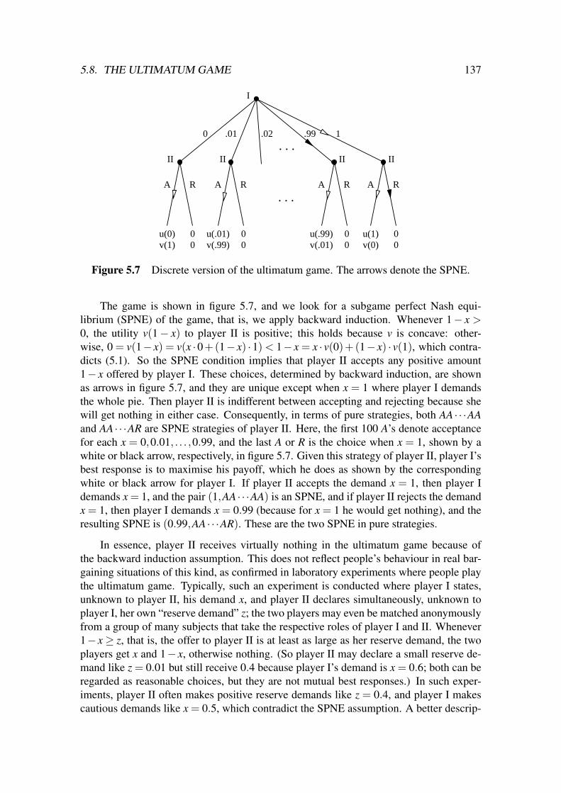
5.8. THE ULTIMATUM GAME 137
A R
v(1)00
A R
u(.01)v(.99)
00
.010
II II
I
.02
u(0)
.99 1
A R
u(.99)v(.01)
00
II
A R
u(1)v(0)
00
II. . .
. . .
Figure 5.7 Discrete version of the ultimatum game. The arrows denote the SPNE.
The game is shown in figure 5.7, and we look for a subgame perfect Nash equi-librium (SPNE) of the game, that is, we apply backward induction. Whenever 1− x >0, the utility v(1− x) to player II is positive; this holds because v is concave: other-wise, 0 = v(1− x) = v(x ·0+(1− x) ·1) < 1− x = x · v(0)+(1− x) · v(1), which contra-dicts (5.1). So the SPNE condition implies that player II accepts any positive amount1− x offered by player I. These choices, determined by backward induction, are shownas arrows in figure 5.7, and they are unique except when x = 1 where player I demandsthe whole pie. Then player II is indifferent between accepting and rejecting because shewill get nothing in either case. Consequently, in terms of pure strategies, both AA · · ·AAand AA · · ·AR are SPNE strategies of player II. Here, the first 100 A’s denote acceptancefor each x = 0,0.01, . . . ,0.99, and the last A or R is the choice when x = 1, shown by awhite or black arrow, respectively, in figure 5.7. Given this strategy of player II, player I’sbest response is to maximise his payoff, which he does as shown by the correspondingwhite or black arrow for player I. If player II accepts the demand x = 1, then player Idemands x = 1, and the pair (1,AA · · ·AA) is an SPNE, and if player II rejects the demandx = 1, then player I demands x = 0.99 (because for x = 1 he would get nothing), and theresulting SPNE is (0.99,AA · · ·AR). These are the two SPNE in pure strategies.
In essence, player II receives virtually nothing in the ultimatum game because ofthe backward induction assumption. This does not reflect people’s behaviour in real bar-gaining situations of this kind, as confirmed in laboratory experiments where people playthe ultimatum game. Typically, such an experiment is conducted where player I states,unknown to player II, his demand x, and player II declares simultaneously, unknown toplayer I, her own “reserve demand” z; the two players may even be matched anonymouslyfrom a group of many subjects that take the respective roles of player I and II. Whenever1− x≥ z, that is, the offer to player II is at least as large as her reserve demand, the twoplayers get x and 1− x, otherwise nothing. (So player II may declare a small reserve de-mand like z = 0.01 but still receive 0.4 because player I’s demand is x = 0.6; both can beregarded as reasonable choices, but they are not mutual best responses.) In such exper-iments, player II often makes positive reserve demands like z = 0.4, and player I makescautious demands like x = 0.5, which contradict the SPNE assumption. A better descrip-

138 CHAPTER 5. BARGAINING
tion of these experiments may therefore be Nash equilibria that are not subgame perfect,with “threats” by player II to reject offers 1−x that are too low. Nevertheless, we assumeSPNE because they allow definite conclusions, and because the model will be refined, andmade more realistic, by allowing rejections to be followed by “counter-demands”.
The described two SPNE of the discrete ultimatum game are found whenever the unitpie can be split into M + 1 possible splits (x,1− x) for x = i/M, for i = 0,1, . . . ,M−1,M, like M = 100 above. Of her 2M+1 pure strategies, player II can play only two inan SPNE, namely always choosing A whenever x < 1, and either A or R in response tox = 1. The respective demand by player I is x = 1 or x = 1− 1/M. With a very finediscretisation where M becomes very large, these two SPNE are nearly identical, withplayer I demanding all (or nearly all) of the pie, and player II receiving almost nothing.
⇒ Exercise 5.3 on page 152 asks you to find all Nash equilibria of the ultimatum game.
0
I
1
. . . A R
u(x)v(1−x)
00
II
x
Figure 5.8 Continuous version of the ultimatum game.
In the “continuous” version of the ultimatum game, the possible demand x by player Iis any number in the interval [0,1], which defines an infinite number of strategies forplayer I. The strategies for player II are even more complicated, namely given by afunction f : [0,1]→ {A,R}, where f (x) = A means that player II accepts the demand x,and f (x) = R means that player II rejects it. (Equivalently, a strategy of player II is anarbitrary subset of [0,1] which consists exactly of those demands x that she accepts.) Thisinfinite game is indicated in figure 5.8. The infinitely many choices x are indicated by thetriangle, whose baseline represents the interval [0,1]. Every point of that baseline has aseparate decision point for player II where she can decide between A and R. Only a singledecision point is drawn in the picture.
We want to show that the continuous ultimatum game has a unique SPNE. Thisrequires an additional assumption, namely that the utility function u of player I is strictlyincreasing.
We first show that concavity of u implies that u is strictly increasing on an interval[0,x′], where u(x) = 1 for all x with x′≤ x≤ 1, so that u is constant on the interval [x′,x]. In

5.9. ALTERNATING OFFERS OVER TWO ROUNDS 139
particular, if x′= 1, then u is increasing throughout. Above, we have shown that because vis concave, v(1−x) cannot be zero if 1−x > 0 because then v would be constant between0 and 1− x and the graph of the function would be below the line connecting the points(0,v(0)) and (1,v(1)). By the same reasoning, u cannot be constant on an interval [x′,x′′]unless x′′ = 1 and u takes constant value 1 on that interval, because a line connecting thetwo points (x′,u(x′)) and (1,u(1)) of the graph of u would have points above the graph.So for all x′,x′′ with x′ < x′′ < 1, we have u(x′) < u(x′′), which means that u is strictlyincreasing.
In the case where u(x′) = 1 holds for some x′ < 1, player I is perfectly satisifed byreceiving only x′, which is less than a full share of the pie. Then any demand x withx′ ≤ x < is accepted by player II because she receives v(1− x) > 0, and x is a possiblestrategy of player I in an SPNE. In that case, we do not get a unique SPNE. We thereforerequire that u is strictly increasing, or equivalently (as explained, because u is concave)that u(x) = 1 implies x = 1. So we make this additional assumption, and similarly assumethat player II’s utility function v is strictly increasing.
We claim that the only SPNE of the continuous ultimatum game is where player Idemands the whole pie, with x = 1, and where player II accepts any demand, includingthe demand x = 1 on the equilibrium path where she is indifferent between acceptingand rejecting. Clearly, this is one SPNE of the game, but why is there no other? Oneargument is that this is the only “limit” of the two SPNE found in any discretised versionof the game. A direct reasoning is as follows. Clearly, player II has to accept wheneverx < 1 because then she receives a positive payoff v(1− x). Suppose there is an SPNEwhere player I’s demand is x so that x < 1. Because u is strictly increasing, player I wouldget more by demanding a little more, but still less than 1, for example (x + 1)/2, whichplayer II still accepts. So x = 1 is the only strategy by player I in an SPNE. Then onthe equilibrium path, player II is indifferent, and can choose either A or R in response tox = 1, and in fact she could randomise between A and R. Suppose that R is played withany positive probability ε > 0, giving player I expected payoff (1−ε)u(1)+εu(0), whichis 1− ε . But then player I’s best response to that strategy of player II would not be x = 1.Instead, player I could improve his payoff, for example by demanding 1− ε/2 becausethen player II would accept for sure and player I receives u(1− ε/2) ≥ 1− ε/2 > 1− ε .However, no demand less than 1 is possible in an SPNE, as we saw earlier.
⇒ Show that concavity of u implies the inequality u(1− ε/2) ≥ 1− ε/2 stated in thepreceding paragraph.
In summary, with demands that can be chosen continuously, the demand of a playerin an SPNE makes the other player indifferent between accepting and rejecting, which theother player nevertheless accepts with certainty. This will also be the guiding principle inSPNE of more complicated games, which we study next.
5.9 Alternating offers over two rounds
Next, we extend the bargaining model so that once a player has rejected the demand ofthe other player, she can make a counter-demand that, in turn, the other player can accept

140 CHAPTER 5. BARGAINING
or reject. In order to find an SPNE of this game by backward induction, these alternatingoffers have to end after some time. The simplest case is bargaining over two rounds,discussed in this section. In the first round, player I makes a demand x, which player IIcan accept or reject. In the latter case, she can make a counter-demand y that representsthe share of the pie she claims for herself, so the pie is split into 1− y for player I andy for player II. If player I accepts that demand, he receives utility u(1− y) and player IIutility v(y). If player I rejects the final demand, both players receive zero.
0
I
1
. . .
II
1
. . . A R
u(1−y)v(y)
00
I
y0
00
u(x)v(1−x)
II
x
A R
δ1−δ
Figure 5.9 Two-round bargaining with a chance move with probability δ that a secondround takes place.
In this game, player II can make the demand in the final round, which is the ultimatumgame with the roles of the players exchanged. In that game, player II can demand thewhole pie, so there would be no reason for her to accept anything offered to her in thefirst round. For that reason, the model has an additional feature shown in figure 5.9.Namely, when player II rejects the first demand, there is a positive probability 1− δthat bargaining terminates with no agreement, where we assume 0 < δ < 1. This is theunsuccessful outcome, with payoff zero to both, given as the result of a chance move. Thegame proceeds to player II’s counter-demand only with probability δ .
By computing expected values, the chance move can be eliminated from the game,which gives the game in figure 5.10. In that game, the pair (u(1− y),v(y)) of utilitieswhen agreement is reached in the second round is multiplied by δ , which is a reduction

5.9. ALTERNATING OFFERS OVER TWO ROUNDS 141
0
I
1
. . .
u(x)v(1−x)
II
x
A R
II
1
. . . A R
u(1−y) 00
I
y0
v(y)δδ
Figure 5.10 The game of figure 5.9 with δ as discount factor applied to second-roundutility values.
of the payoffs because δ < 1. The usual interpretation of δ is that of a discount factor,which expresses that later payoffs are worth less than earlier payoffs.
A discount factor applied to future payoffs is realistic. In monetary terms, it canexpress lost interest payments (for money today as opposed to money in the future). Moreimportantly, future payoffs are less secure because, for example, the buyer or seller in adeal may change his or her mind, or because of other unforeseen circumstances. This ismodelled with the chance move in figure 5.9. In addition, this chance move provides agood reason why both players have the same discount factor. Alternatively, one may usedifferent discount factors δI and δII for the two players, which give second-round payoffsδIu(1− y) and δIIv(y). If these discount factors are different, a higher discount factorrepresents a more patient player because his or her future payoff would differ less fromthe present payoff. However, the resulting game would be more complicated to analyse,and it would be more difficult to establish a connection to the Nash bargaining solution.For that reason, we use only one discount factor, in agreement with the model that δrepresents the probability that bargaining continues into the next round.
An SPNE of the game is found as follows. By backward induction, we have toanalyse the last round first. When player II makes her demand y to player I, he can onlyaccept or reject. This is the ultimatum game analysed earlier, so player II demands thewhole pie y = 1, and player I accepts any offer made to him, in particular this demandy = 1 (recall that player I’s strategy is a function of the demand y that he faces), andplayer I will get nothing. Here, it does not matter if the last stage represents the subgame

142 CHAPTER 5. BARGAINING
starting with player II’s demand y in figure 5.9, or the same game with discounted payoffsin figure 5.10, because the latter payoffs are merely scaled with the positive scalar δ , sothese are the same games in strategic terms, with the same equilibria. In either game,backward induction shows that if player II rejects player I’s demand x in the first roundand chooses R, the payoffs for both players are zero for player I, and δv(1), which is δ ,for player II.
According to the next backward induction step, what should player I do in the firstround? Player II’s reaction is unique except when she is indifferent. This means that shewill accept if she is offered a utility v(1− x) (now undiscounted, because this is the firstround) that exceeds the amount δ that she can expect to get by rejection; she is indifferentif v(1− x) = δ ; and she will reject if v(1− x) < δ . By the same reasoning as that usedin the continuous ultimatum game, the demand x by player I in the SPNE is chosen sothat v(1− x) = δ , and player II accepts on the equilibrium path. (If she did not accept,player I would offer her a little bit more and make her accept, but player I must make herindifferent in order to obtain an SPNE.)
The resulting SPNE is unique. Player I demands x so that v(1− x) = δ , which isaccepted immediately by player II, so that the game terminates with player I receivingu(x) and player II receiving v(1− x), which is equal to δ . The full equilibrium strategiesare (with this x): Player II accepts any demand x′ so that 0≤ x′ ≤ x, and rejects any x′ > x.Any counter-demand by player II in the second round is y = 1, and player I accepts anyamount in the second round. The strategies have to specify the actions of the players inthe second stage in order to perform the backward induction analysis.
1
u
v
10 δ
δA B
Figure 5.11 Graphical solution of the two-round bargaining game in figure 5.10. Theinner curve is the set of discounted payoff pairs for the second round.
Player I’s demand x in the first round is easily found graphically as shown in fig-ure 5.11. This shows, as the outer curve, the Pareto-frontier of the bargaining set, herefor the utility functions u(x) =
√x and v(y) = y used earlier. Recall that for 0 ≤ x ≤ 1,
one obtains any point (u(x),v(1− x)) on that Pareto-frontier. Multiplying any such pairof real numbers with the factor δ gives a “shrunk” version of the Pareto-frontier, shown
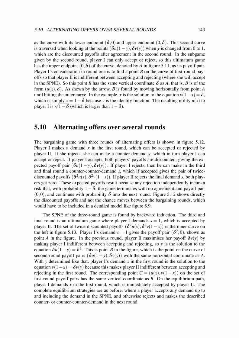
5.10. ALTERNATING OFFERS OVER SEVERAL ROUNDS 143
as the curve with its lower endpoint (δ ,0) and upper endpoint (0,δ ). This second curveis traversed when looking at the points (δu(1− y),δv(y)) when y is changed from 0 to 1,which are the discounted payoffs after agreement in the second round. In the subgamegiven by the second round, player I can only accept or reject, so this ultimatum gamehas the upper endpoint (0,δ ) of the curve, denoted by A in figure 5.11, as its payoff pair.Player I’s consideration in round one is to find a point B on the curve of first-round pay-offs so that player II is indifferent between accepting and rejecting (where she will acceptin the SPNE). So this point B has the same vertical coordinate δ as A, that is, B is of theform (u(x),δ ). As shown by the arrow, B is found by moving horizontally from point Auntil hitting the outer curve. In the example, x is the solution to the equation v(1−x) = δ ,which is simply x = 1−δ because v is the identity function. The resulting utility u(x) toplayer I is
√1−δ (which is larger than 1−δ ).
5.10 Alternating offers over several rounds
The bargaining game with three rounds of alternating offers is shown in figure 5.12.Player I makes a demand x in the first round, which can be accepted or rejected byplayer II. If she rejects, she can make a counter-demand y, which in turn player I canaccept or reject. If player I accepts, both players’ payoffs are discounted, giving the ex-pected payoff pair (δu(1− y),δv(y)). If player I rejects, then he can make in the thirdand final round a counter-counter-demand s, which if accepted gives the pair of twice-discounted payoffs (δ 2u(s),δ 2v(1− s)). If player II rejects the final demand s, both play-ers get zero. These expected payoffs result because any rejection independently incurs arisk that, with probability 1− δ , the game terminates with no agreement and payoff pair(0,0), and continues with probability δ into the next round. Figure 5.12 shows directlythe discounted payoffs and not the chance moves between the bargaining rounds, whichwould have to be included in a detailed model like figure 5.9.
The SPNE of the three-round game is found by backward induction. The third andfinal round is an ultimatum game where player I demands s = 1, which is accepted byplayer II. The set of twice discounted payoffs (δ 2u(s),δ 2v(1− s)) is the inner curve onthe left in figure 5.13. Player I’s demand s = 1 gives the payoff pair (δ 2,0), shown aspoint A in the figure. In the previous round, player II maximises her payoff δv(y) bymaking player I indifferent between accepting and rejecting, so y is the solution to theequation δu(1− y) = δ 2. This is point B in the figure, which is the point on the curve ofsecond-round payoff pairs (δu(1− y),δv(y)) with the same horizontal coordinate as A.With y determined like that, player I’s demand x in the first round is the solution to theequation v(1−x) = δv(y) because this makes player II indifferent between accepting andrejecting in the first round. The corresponding point C = (u(x),v(1− x)) on the set offirst-round payoff pairs has the same vertical coordinate as B. On the equilibrium path,player I demands x in the first round, which is immediately accepted by player II. Thecomplete equilibrium strategies are as before, where a player accepts any demand up toand including the demand in the SPNE, and otherwise rejects and makes the describedcounter- or counter-counter-demand in the next round.

144 CHAPTER 5. BARGAINING
u(x)v(1−x)
I
y0
II
1
u(1−y)v(y)
I
II
s 10
u(s)2
2v(1−s)
I
II
A R
0 1x
. . .A R
A R. . .
00
. . .
δδ
δδ
Figure 5.12 Bargaining over three rounds.
The game with four bargaining rounds has the same structure as the game with threerounds, except that if player II rejects player I’s demand s in round three, she can makea final demand t of her own in the fourth and final round, which player I can only ac-cept or reject. If player I accepts, the players receive the three-times discounted payoffs(δ 3u(1− t),δ 3v(t)). The corresponding SPNE is solved graphically as shown on theright in figure 5.13. The last round is an ultimatum game where player II can demandthe whole pie with t = 1, which determines the payoff pair (0,δ 3), which is point A inthe figure. In the previous round, the third round of the game, player I demands s so thatplayer II is indifferent between accepting and rejecting, which gives point B, which isthe pair of discounted payoffs (δ 2u(s),δ 2v(1− s)) so that δ 2v(1− s) = δ 3. In the roundbefore that, player II makes player I indifferent between accepting and rejecting with thedemand y so that δu(1− y) = δ 2u(s), shown as point C. In the first round, player I de-mands x so as to make player II indifferent, according to v(1− x) = δv(y), which defines
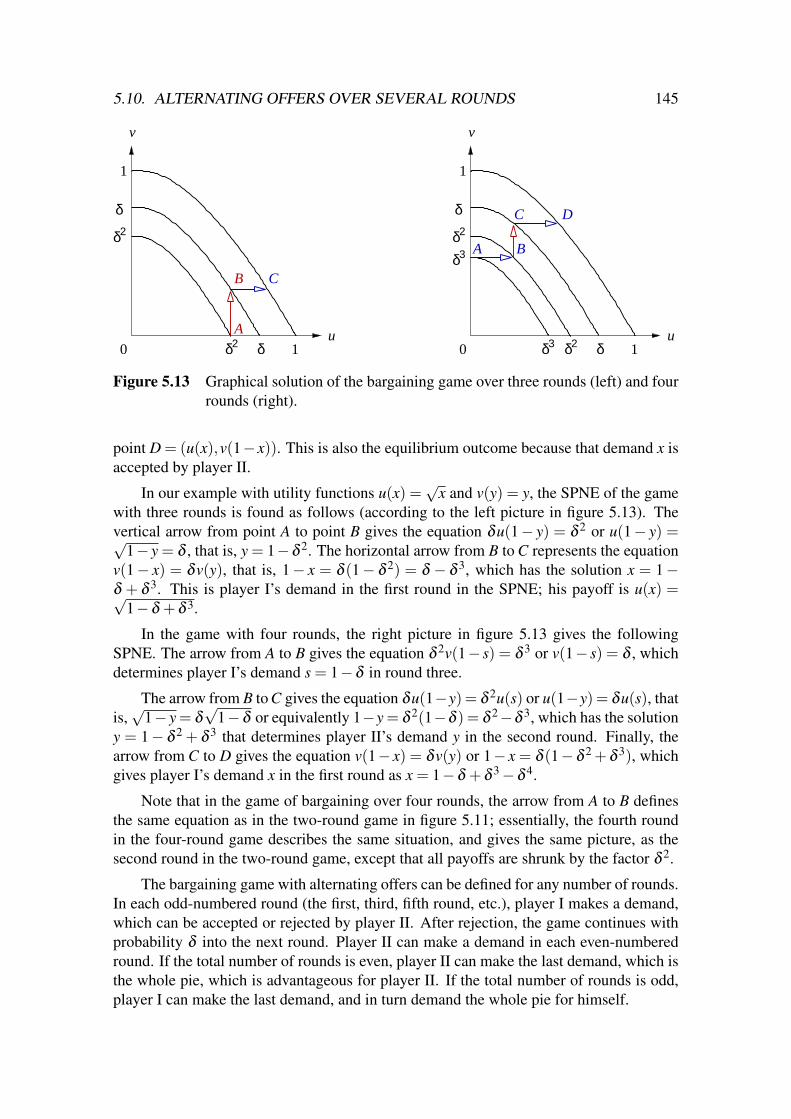
5.10. ALTERNATING OFFERS OVER SEVERAL ROUNDS 145
1
u
v
10 δ
δ
δ2
δ2
A
B C
1
u
v
10 δ
δ
δ2
δ2
δ3
δ3 A
C D
B
Figure 5.13 Graphical solution of the bargaining game over three rounds (left) and fourrounds (right).
point D = (u(x),v(1−x)). This is also the equilibrium outcome because that demand x isaccepted by player II.
In our example with utility functions u(x) =√
x and v(y) = y, the SPNE of the gamewith three rounds is found as follows (according to the left picture in figure 5.13). Thevertical arrow from point A to point B gives the equation δu(1− y) = δ 2 or u(1− y) =√
1− y = δ , that is, y = 1−δ 2. The horizontal arrow from B to C represents the equationv(1− x) = δv(y), that is, 1− x = δ (1− δ 2) = δ − δ 3, which has the solution x = 1−δ + δ 3. This is player I’s demand in the first round in the SPNE; his payoff is u(x) =√
1−δ +δ 3.
In the game with four rounds, the right picture in figure 5.13 gives the followingSPNE. The arrow from A to B gives the equation δ 2v(1− s) = δ 3 or v(1− s) = δ , whichdetermines player I’s demand s = 1−δ in round three.
The arrow from B to C gives the equation δu(1−y) = δ 2u(s) or u(1−y) = δu(s), thatis,√
1− y = δ√
1−δ or equivalently 1−y = δ 2(1−δ ) = δ 2−δ 3, which has the solutiony = 1− δ 2 + δ 3 that determines player II’s demand y in the second round. Finally, thearrow from C to D gives the equation v(1− x) = δv(y) or 1− x = δ (1−δ 2 +δ 3), whichgives player I’s demand x in the first round as x = 1−δ +δ 3−δ 4.
Note that in the game of bargaining over four rounds, the arrow from A to B definesthe same equation as in the two-round game in figure 5.11; essentially, the fourth roundin the four-round game describes the same situation, and gives the same picture, as thesecond round in the two-round game, except that all payoffs are shrunk by the factor δ 2.
The bargaining game with alternating offers can be defined for any number of rounds.In each odd-numbered round (the first, third, fifth round, etc.), player I makes a demand,which can be accepted or rejected by player II. After rejection, the game continues withprobability δ into the next round. Player II can make a demand in each even-numberedround. If the total number of rounds is even, player II can make the last demand, which isthe whole pie, which is advantageous for player II. If the total number of rounds is odd,player I can make the last demand, and in turn demand the whole pie for himself.
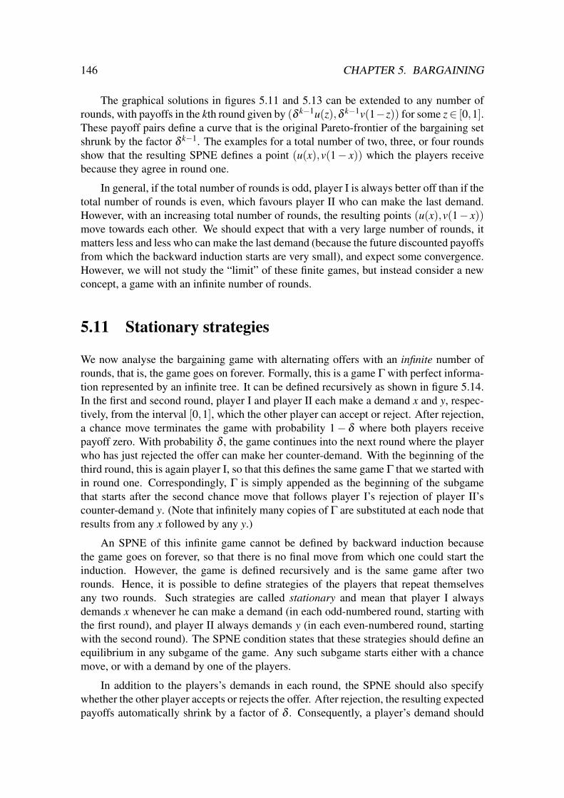
146 CHAPTER 5. BARGAINING
The graphical solutions in figures 5.11 and 5.13 can be extended to any number ofrounds, with payoffs in the kth round given by (δ k−1u(z),δ k−1v(1−z)) for some z∈ [0,1].These payoff pairs define a curve that is the original Pareto-frontier of the bargaining setshrunk by the factor δ k−1. The examples for a total number of two, three, or four roundsshow that the resulting SPNE defines a point (u(x),v(1− x)) which the players receivebecause they agree in round one.
In general, if the total number of rounds is odd, player I is always better off than if thetotal number of rounds is even, which favours player II who can make the last demand.However, with an increasing total number of rounds, the resulting points (u(x),v(1− x))move towards each other. We should expect that with a very large number of rounds, itmatters less and less who can make the last demand (because the future discounted payoffsfrom which the backward induction starts are very small), and expect some convergence.However, we will not study the “limit” of these finite games, but instead consider a newconcept, a game with an infinite number of rounds.
5.11 Stationary strategies
We now analyse the bargaining game with alternating offers with an infinite number ofrounds, that is, the game goes on forever. Formally, this is a game Γ with perfect informa-tion represented by an infinite tree. It can be defined recursively as shown in figure 5.14.In the first and second round, player I and player II each make a demand x and y, respec-tively, from the interval [0,1], which the other player can accept or reject. After rejection,a chance move terminates the game with probability 1− δ where both players receivepayoff zero. With probability δ , the game continues into the next round where the playerwho has just rejected the offer can make her counter-demand. With the beginning of thethird round, this is again player I, so that this defines the same game Γ that we started within round one. Correspondingly, Γ is simply appended as the beginning of the subgamethat starts after the second chance move that follows player I’s rejection of player II’scounter-demand y. (Note that infinitely many copies of Γ are substituted at each node thatresults from any x followed by any y.)
An SPNE of this infinite game cannot be defined by backward induction becausethe game goes on forever, so that there is no final move from which one could start theinduction. However, the game is defined recursively and is the same game after tworounds. Hence, it is possible to define strategies of the players that repeat themselvesany two rounds. Such strategies are called stationary and mean that player I alwaysdemands x whenever he can make a demand (in each odd-numbered round, starting withthe first round), and player II always demands y (in each even-numbered round, startingwith the second round). The SPNE condition states that these strategies should define anequilibrium in any subgame of the game. Any such subgame starts either with a chancemove, or with a demand by one of the players.
In addition to the players’s demands in each round, the SPNE should also specifywhether the other player accepts or rejects the offer. After rejection, the resulting expectedpayoffs automatically shrink by a factor of δ . Consequently, a player’s demand should

5.11. STATIONARY STRATEGIES 147
II
00
0
I
1
. . .
1
. . .
0
u(x)v(1−x)
II
x
A R
00
y
I
A R
u(1−y)v(y)
δ1−δ
δ1−δ
Γ
Figure 5.14 The bargaining game Γ with an infinite number of rounds, which repeatsitself after any demand x of player I in round one and any demand y ofplayer II in round two after each player has rejected the other’s demand;each time, the next round is reached with probability δ .
not be so high as to result in rejection, but should instead make it optimal for the otherplayer to accept. The demand itself is maximal subject to this condition, that is, it is, asbefore, chosen so as to make the other player indifferent between accepting and rejecting,and the other player accepts in the SPNE.
We now show that an SPNE exists, and how to find it, using a graph similar to the leftpicture in figure 5.13. Like there, we draw the three curves of payoff pairs (u(x),v(1−x))resulting from player I’s demand x in round one if this demand is accepted by player II,the discounted payoffs δ (u(1− y),δv(y)) if player I accepts player II’s demand y in roundtwo, and the third-round twice-discounted payoffs δ 2(u(s),δ 2v(1− s)) if player II acceptsplayer I’s demand s in round three. The demands x and y are chosen so as to make theother player indifferent between acceptance and rejection. For the demand s in roundthree, we want to fulfil the requirement of stationary strategies, that is, s = x.
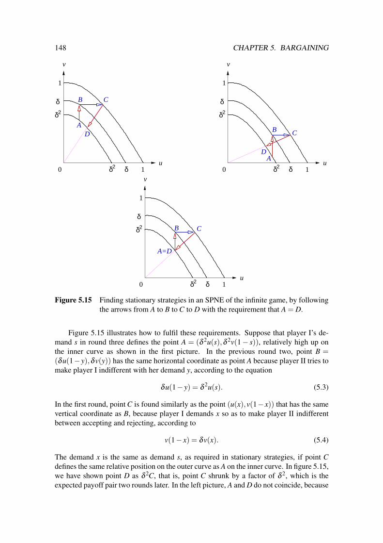
148 CHAPTER 5. BARGAINING
1
u
v
10 δ
δ
δ2
δ2
A
B C
D
1
u
v
10 δ
δ
δ2
δ2
AD
CB
1
u
v
10 δ
δ
δ2
δ2 B C
A=D
Figure 5.15 Finding stationary strategies in an SPNE of the infinite game, by followingthe arrows from A to B to C to D with the requirement that A = D.
Figure 5.15 illustrates how to fulfil these requirements. Suppose that player I’s de-mand s in round three defines the point A = (δ 2u(s),δ 2v(1− s)), relatively high up onthe inner curve as shown in the first picture. In the previous round two, point B =(δu(1−y),δv(y)) has the same horizontal coordinate as point A because player II tries tomake player I indifferent with her demand y, according to the equation
δu(1− y) = δ 2u(s). (5.3)
In the first round, point C is found similarly as the point (u(x),v(1−x)) that has the samevertical coordinate as B, because player I demands x so as to make player II indifferentbetween accepting and rejecting, according to
v(1− x) = δv(x). (5.4)
The demand x is the same as demand s, as required in stationary strategies, if point Cdefines the same relative position on the outer curve as A on the inner curve. In figure 5.15,we have shown point D as δ 2C, that is, point C shrunk by a factor of δ 2, which is theexpected payoff pair two rounds later. In the left picture, A and D do not coincide, because

5.11. STATIONARY STRATEGIES 149
s < x, that is, the third-round demand s was too small. The second picture in figure 5.15shows a point A on the inner curve corresponding to a demand s that is too favourable forplayer I, where the arrows from A to B to C according to equations (5.3) and (5.4) give afirst-round demand x with x < s.
In general, the pictures demonstrate that when starting from s = 0, these equationsgive a first-round demand x where x > s, and when starting from s = 1, a first-rounddemand x where x < s. (Note that these extreme starting points s = 0 and s = 1 giveexactly the solutions of bargaining over two and three rounds, respectively.) Moreover,when starting from any s in [0,1], the resulting demand x is a continuous function of s.Because the continuous function x− s is positive for s = 0 and negative for s = 1, it iszero for some intermediate value s, where s = x, which defines a stationary SPNE.
In short, the stationary SPNE of the infinite bargaining game is a solution to the equa-tions (5.3), (5.4), and s = x. These are equivalent to the two, nicely symmetric equations
u(1− y) = δu(x), v(1− x) = δv(y). (5.5)
The first of these equations expresses that player II makes player I indifferent in everyeven-numbered round by her demand y. The second equation in (5.5) states that player Imakes player II indifferent by his demand x in every odd-numbered round. In this sta-tionary SPNE, player I’s demand x in round one is immediately accepted by player II.As before, the full strategies specify acceptance of any lower and rejection of any higherdemand. The actual demand of the other player is always accepted, so the later rounds arenever reached.
In the example with utility functions u(x) =√
x and v(y) = y, the stationary strategiesin an SPNE are found as follows. They are given by the demands x and y that solve (5.5),that is, √
1− y = δ√
x, 1− x = δy.
The first equation is equivalent to y = 1−δ 2x, which substituted into the second equationgives 1− x = δ −δ 3x, or 1−δ = x(1−δ 3). Because 1−δ 3 = (1−δ )(1+δ +δ 2), thisgives the solutions for x and y as
x =1−δ1−δ 3 =
11+δ +δ 2 , y =
1+δ1+δ +δ 2 . (5.6)
The pie is split in the first round into x = 1/(1 + δ + δ 2) for player I and 1− x = (δ +δ 2)/(1 + δ + δ 2) for player II. The share 1− x of the pie for player II is lower than herdemand y in the second round, as illustrated by the last picture in figure 5.15, which showsthat the relative position of point A on the outer curve is higher than that of point B on themiddle curve. This holds because the second-round payoffs are discounted.
Does it matter for our analysis that player I makes the first demand? Of course, ifplayer II made the first demand, one could swap the players and analyse the game withthe described method. However, the game where player II makes the first demand, and thecorresponding stationary solution, is already analysed as part of the game Γ where player Imoves first. The reason is that the game with player II moving first is the subgame of Γin figure 5.14 after the first chance move, which repeats itself as in Γ. All we would have
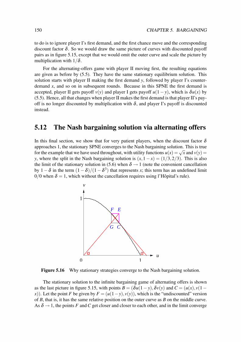
150 CHAPTER 5. BARGAINING
to do is to ignore player I’s first demand, and the first chance move and the correspondingdiscount factor δ . So we would draw the same picture of curves with discounted payoffpairs as in figure 5.15, except that we would omit the outer curve and scale the picture bymultiplication with 1/δ .
For the alternating-offers game with player II moving first, the resulting equationsare given as before by (5.5). They have the same stationary equilibrium solution. Thissolution starts with player II making the first demand y, followed by player I’s counter-demand x, and so on in subsequent rounds. Because in this SPNE the first demand isaccepted, player II gets payoff v(y) and player I gets payoff u(1− y), which is δu(x) by(5.5). Hence, all that changes when player II makes the first demand is that player II’s pay-off is no longer discounted by multiplication with δ , and player I’s payoff is discountedinstead.
5.12 The Nash bargaining solution via alternating offers
In this final section, we show that for very patient players, when the discount factor δapproaches 1, the stationary SPNE converges to the Nash bargaining solution. This is truefor the example that we have used throughout, with utility functions u(x) =
√x and v(y) =
y, where the split in the Nash bargaining solution is (x,1− x) = (1/3,2/3). This is alsothe limit of the stationary solution in (5.6) when δ → 1 (note the convenient cancellationby 1− δ in the term (1− δ )/(1− δ 3) that represents x; this term has an undefined limit0/0 when δ = 1, which without the cancellation requires using l’Hopital’s rule).
αα
1
v
10u
G
F E
C
Figure 5.16 Why stationary strategies converge to the Nash bargaining solution.
The stationary solution to the infinite bargaining game of alternating offers is shownas the last picture in figure 5.15, with points B = (δu(1− y),δv(y) and C = (u(x),v(1−x)). Let the point F be given by F = (u(1−y),v(y)), which is the “undiscounted” versionof B, that is, it has the same relative position on the outer curve as B on the middle curve.As δ → 1, the points F and C get closer and closer to each other, and in the limit converge
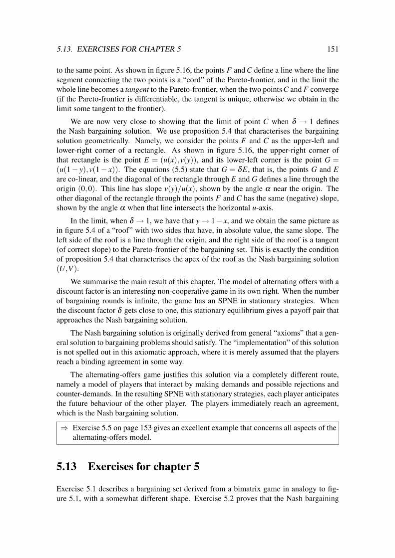
5.13. EXERCISES FOR CHAPTER 5 151
to the same point. As shown in figure 5.16, the points F and C define a line where the linesegment connecting the two points is a “cord” of the Pareto-frontier, and in the limit thewhole line becomes a tangent to the Pareto-frontier, when the two points C and F converge(if the Pareto-frontier is differentiable, the tangent is unique, otherwise we obtain in thelimit some tangent to the frontier).
We are now very close to showing that the limit of point C when δ → 1 definesthe Nash bargaining solution. We use proposition 5.4 that characterises the bargainingsolution geometrically. Namely, we consider the points F and C as the upper-left andlower-right corner of a rectangle. As shown in figure 5.16, the upper-right corner ofthat rectangle is the point E = (u(x),v(y)), and its lower-left corner is the point G =(u(1− y),v(1− x)). The equations (5.5) state that G = δE, that is, the points G and Eare co-linear, and the diagonal of the rectangle through E and G defines a line through theorigin (0,0). This line has slope v(y)/u(x), shown by the angle α near the origin. Theother diagonal of the rectangle through the points F and C has the same (negative) slope,shown by the angle α when that line intersects the horizontal u-axis.
In the limit, when δ → 1, we have that y→ 1− x, and we obtain the same picture asin figure 5.4 of a “roof” with two sides that have, in absolute value, the same slope. Theleft side of the roof is a line through the origin, and the right side of the roof is a tangent(of correct slope) to the Pareto-frontier of the bargaining set. This is exactly the conditionof proposition 5.4 that characterises the apex of the roof as the Nash bargaining solution(U,V ).
We summarise the main result of this chapter. The model of alternating offers with adiscount factor is an interesting non-cooperative game in its own right. When the numberof bargaining rounds is infinite, the game has an SPNE in stationary strategies. Whenthe discount factor δ gets close to one, this stationary equilibrium gives a payoff pair thatapproaches the Nash bargaining solution.
The Nash bargaining solution is originally derived from general “axioms” that a gen-eral solution to bargaining problems should satisfy. The “implementation” of this solutionis not spelled out in this axiomatic approach, where it is merely assumed that the playersreach a binding agreement in some way.
The alternating-offers game justifies this solution via a completely different route,namely a model of players that interact by making demands and possible rejections andcounter-demands. In the resulting SPNE with stationary strategies, each player anticipatesthe future behaviour of the other player. The players immediately reach an agreement,which is the Nash bargaining solution.
⇒ Exercise 5.5 on page 153 gives an excellent example that concerns all aspects of thealternating-offers model.
5.13 Exercises for chapter 5
Exercise 5.1 describes a bargaining set derived from a bimatrix game in analogy to fig-ure 5.1, with a somewhat different shape. Exercise 5.2 proves that the Nash bargaining

152 CHAPTER 5. BARGAINING
solution obtained by maximising the Nash product actually fulfils one of the required ax-ioms. Exercise 5.3 considers a discrete ultimatum game similar to figure 5.7, where youare asked in (d) to find all its Nash equilibria; not all of these are SPNE, so they may in-volve the “threat” of rejecting an offer that would be accepted in an SPNE. Exercises 5.4and 5.5 consider the problem of splitting a unit pie with a specific pair of utility functions,and the iterated-offers bargaining game.
Exercise 5.1 Draw the convex hull of payoff pairs for the following 2× 2 game. Whatis the threat point? Show the bargaining set derived from this game, as explained insection 5.4. Indicate the Pareto-frontier. Find the Nash bargaining solution (U,V ).
@@@I
II
T
B
l r
3 2
4 1
4 1
3 1
Exercise 5.2 Consider a bargaining set S with threat point (0,0). Let a > 0, b > 0, andlet S′ = {(au,bv) | (u,v) ∈ S}. The set S′ is the set of utility pairs in S rescaled by afor player I and by b for player II. Recall that one axiomatic property of the bargainingsolution is independence from these scale factors.
Show that the Nash product fulfils this property, that is, the Nash bargaining solutionfrom S obtained by maximising the Nash product re-scales to become the solution for S′.
Note: Don’t panic! This is extremely easy once you state in the right way what itmeans that something maximises something. You may find it useful to consider first thesimpler case b = 1.
Exercise 5.3 We repeat the definition of the discretised ultimatum game. Let M be apositive integer. Player I’s possible actions are to ask for a number x, called his demand,which is one of the (integer) numbers 0,1,2, . . . ,M. In response to this demand, player IIcan either accept (A) or reject (R). When player II accepts, then player I will receive apayoff of x and player II a payoff of M− x. When player II rejects, both players receivepayoff zero.
(a) Draw the game tree for this game, as an extensive game with perfect information, forM = 3.
(b) What is the number of pure strategies in this game, for general M, for player I andfor player II? What is the number of reduced pure strategies in this game, for player Iand for player II?
(c) Determine all subgame perfect equilibria of the game in pure strategies.
(d) Determine all Nash equilibria (not necessarily subgame perfect) of this game in purestrategies.

5.13. EXERCISES FOR CHAPTER 5 153
(e) Determine all subgame perfect equilibria of this game where both players may usebehaviour strategies, in addition to those in (c).
Exercise 5.4 Consider the following bargaining problem. In the usual way, a “unit pie”is split into non-negative amounts x and y with x+y≤ 1. The utility function of player I isu(x) = x, the utility function of player II is v(y) = 1− (1− y)2. The threat point is (0,0).
(a) Draw the bargaining set (as set of possible utilities (u,v)) and indicate the Pareto-frontier in the picture.
(b) Find the Nash bargaining solution. How will the pie be split, and what are the utilitiesof the players?
Exercise 5.5 Consider the bargaining problem of splitting a unit pie with utility functionsu,v: [0,1]→ [0,1] as in exercise 5.4, that is, u(x) = x and v(y) = 1− (1− y)2. Assumenow that the bargaining outcome is determined by the subgame perfect equilibrium ofthe standard alternating-offers bargaining game with k rounds. In round 1 player I makesa certain demand. If player II rejects this, she can make a certain counter-demand inround 2, and so on. A rejection in the last round k means that both players get nothing.The last player to make a demand is player I if k is odd, and player II if k is even. Whenagreement takes place in round i for some i with 1 ≤ i ≤ k, then the bargaining set hasshrunk by a factor of δ i−1. That is, the utility of what the players can get after each roundof rejection is reduced by multiplication with the discount factor δ .
(a) Suppose that the number of rounds is k = 2. Draw the picture of shrinking bargainingsets (for some choice of δ ) in these two rounds. Find the subgame perfect equilib-rium, in terms of player I’s demand x, for general δ . What is the demand x whenδ = 3/4? What are the strategies of the two players in this subgame perfect equilib-rium?
(b) Suppose that the number of rounds is k = 3. Draw the picture of shrinking bargain-ing sets in these three rounds. Find the subgame perfect equilibrium, for general δ ,computing the demand of player I in round 1 (you do not need to specify the players’strategies). What is player I’s demand x when δ = 1/4? (Then x happens to be arational number.)
(c) Consider now an infinite number of rounds, and look for stationary equilibrium strate-gies, where player I demands the same amount x each time he makes a demand, andplayer II demands the same amount y every time she makes a demand. What is thisdemand x when δ = 3/5? What is the demand x when δ goes to 1? Compare thiswith the result of exercise 5.4(b).

154 CHAPTER 5. BARGAINING

Chapter 6
Geometric representation of equilibria
This chapter is an extension of the lecture notes “Game Theory Basics” on topics that havebeen first taught in autumn 2010. It comprises about one week of lectures that partiallyreplace the old chapter 5 on bargaining, and follows on from section 3.13.
In this chapter we consider a geometric method to identify the Nash equilibria of atwo-player game with up to three strategies per player, and provide an existence proofof Nash equilibria for nondegenerate two-player games known as the “Lemke–Howsonalgorithm”.
6.1 Learning objectives
After studying this chapter, you should be able to:
• draw best response diagrams for bimatrix games with up three strategies per player;
• identify the Nash equilibria of the game with the help of the labels used in thesediagrams, and explain the connection of labels and the best response condition;
• show the computation of one Nash equilibrium with the Lemke–Howson algorithmusing the diagram.
6.2 Further reading
The best response diagrams are to my knowledge not found in undergraduate textbooks.A general description of the Lemke–Howson algorithm is found in my chapter of a post-graduate textbook,
• B. von Stengel (2007), Equilibrium computation for two-player games in strategicand extensive form. Chapter 3 of Algorithmic Game Theory, eds. N. Nisan, T. Rough-garden, E. Tardos, and V. Vazirani, Cambridge Univ. Press, Cambridge, pages 53–78.
155

156 CHAPTER 6. GEOMETRIC REPRESENTATION OF EQUILIBRIA
6.3 Introduction
The following sections present methods for finding Nash equilibria in mixed strategies fortwo-player games in strategic form.
We recall the notation used in chapter 3. Player I has m and player II has n strategies.For any pair (i, j) of strategies, each player receives a payoff, which is independent ofthe payoff to the other player. In particular, we do not require the zero-sum property. Asusual, the m strategies of player I can be considered as rows and the n pure strategiesof player II as columns in a table representing the strategic form. The game is thencompletely specified by two m×n matrices A and B containing the payoffs to player I andplayer II, respectively. The game is therefore also called a bimatrix game, given by thematrix pair (A,B).
In the following, we give a geometric illustration of equilibria for such bimatrixgames. This is particularly helpful for games with up to three pure strategies per player,in particular 3×3 games, and can even be pictured (although less easily drawn) if a playerhas four strategies. A number of considerations can be demonstrated with 3× 3 gameswhich would be too simple or pointless with 2×2 games, so that this geometric approachis very useful.
Given this geometric approach, we will then present an algorithm – a systematicmethod which can be performed by a computer – for finding one equilibrium of a bimatrixgame, known as the Lemke–Howson algorithm. This method provides also a constructiveand elementary proof that every bimatrix has at least one equilibrium. Moreover, themethod shows that a nondegenerate bimatrix game has always an odd number of Nashequilibria.
6.4 Best response regions
Consider an m×n bimatrix game (A,B), with payoff matrix A for the row player (player I)and B for the column player (player II). Throughout, we will use as an example the 3×3game
A =
0 3 01 0 1−3 4 5
, B =
0 1 −22 0 32 1 0
. (6.1)
Note, however, that the presented method does not require that both players have the samenumber of pure strategies. That is, m 6= n is quite possible. In that respect, a 3×2 game,for example, would be more typical, but this would be less suitable to illustrate the powerof the construction.
The first step of the construction is a unique numbering of the pure strategies of theplayers to identify them more easily. Let the set of pure strategies of player I be given by
M = {1, . . . ,m}

6.4. BEST RESPONSE REGIONS 157
and the set of pure strategies of player II by
N = {m+1, . . . ,m+n}.
That is, the numbering of the strategies is continued for player II to produce two disjointsets M and N. The pure strategies will be used to identify equilibria by considering themas labels of certain geometrically defined sets. That is, a label is defined as an element ofM∪N. We will circle these numbers to identify them as such labels. In our example (6.1)we therefore have
M = {©1 ,©2 ,©3 }, N = {©4 ,©5 ,©6 }.It is helpful to mark the rows of A with the pure strategies©1 ,©2 ,©3 of player I and thecolumns of B with the pure strategies©4 ,©5 ,©6 of player II (that is, writing©1 ,©2 ,©3 tothe left of A and©4 ,©5 ,©6 at the top of B).
The second step is the geometric representation of the sets of mixed strategies ofplayer I and player II which we recall from section 3.8. A mixed strategy of player I isa probability distribution on the set M of his pure strategies. This is an m-dimensionalvector x with nonnegative components xi for i in M that sum up to one. In the samemanner, y is a mixed strategy of player II if it has n nonnegative components y j for j inN with ∑ j∈N y j = 1. The sets X and Y of mixed strategies of player I and II are thereforedefined as
X = {x ∈ RM | ∑i∈M
xi = 1, xi ≥ 0 for i ∈M},
Y = {y ∈ RN | ∑j∈N
y j = 1, y j ≥ 0 for j ∈ N}.
We use here the notation RN instead of Rn to indicate that the components y j of a vector yin RN have the elements j in N has subscripts, which are here not the first n natural num-bers, but, according to the above definition of N, the numbers m+1, . . . ,m+n. Instead ofRM one could also write Rm.
For n = 3 as in the above example (6.1) the set Y is the set of all convex combinations
of the unit vectors
100
,
010
,
001
(we use x and y as column vectors). That is, Y is
a triangle, as figure 6.1 illustrates, which is similar to figure 3.4. Note the numbering ofthe components y4,y5,y6 of y.
This triangle is part of the plane that goes through the three unit vectors and is there-fore a two-dimensional geometric figure. For n = 4 one would obtain a tetrahedron, forn = 2 merely a line segment. In general, the “convex hull” of the unit vectors is calleda simplex. This geometric object has one dimension less than the space containing theunit vectors ander consideration, because the components of any vector contained in thatsimplex add up to one, that is, they fulfill one linear equation.
The third and most important step in the construction is the subdivision of the strat-egy sets into best response regions. Such a best response region is that set of mixedstrategies of a player where a pure strategy of the other player is a best response. Wefirst illustrate this with our example (6.1) with n = 3 and consider a mixed strategy y

158 CHAPTER 6. GEOMETRIC REPRESENTATION OF EQUILIBRIA
-¡
¡¡
¡¡
¡¡
¡¡ª
6
££
££
££
££
££
££
££
£££³³³³³³³³³³³³³³³³³@
@@
@@
@@
@@
@@
y4
y5
y6
Figure 6.1 Mixed strategy simplex of player II for a 3×3 game.
of player II. Then y = (y4,y5,y6)>, where the superscript “>” means transposition, towrite the column vector y as a transposed row vector. For given y, player I has the purestrategies©1 ,©2 and©3 as possible reponses and then gets the expected payoffs for
©1 : 3y5, ©2 : y4 + y6, ©3 :−3y4 +4y5 +5y6.
When is©1 a best response to y? Apparently when the expected payoff for©1 is at leastas high as that for©2 and©3 , that is, if the inequalities
3y5 ≥ y4 + y6, 3y5 ≥−3y4 +4y5 +5y6 (6.2)
hold, or equivalently3y5 ≥ y4 + y6, 3y4 ≥ y5 +5y6. (6.3)
The inequalities in (6.3) have been obtained by sorting the linear coefficients of the vari-ables y4,y5,y6 so that they appear only once and with positive sign on one side of eachinequality; for example, rather than writing 3y5−y4≥ y6 we write 3y5≥ y4 +y6 by addingy4 on both sides.
The best response region for the strategy ©1 is therefore that subset of Y where theinequalities (6.2) are fulfilled. These are in general m−1 linear inequalities that describethe comparison with the other pure strategies of player I. The general definition of a bestresponse region for a pure strategy i in M of player I is
Y (i) = {y ∈ Y | i is a best response to y}

6.4. BEST RESPONSE REGIONS 159
and correspondingly for a pure strategy j in N of player II
X( j) = {x ∈ X | j is a best response to x},where X( j) is defined by n−1 inequalities.
In addition to these inequalities we have the linear constraints that define Y and X ,respectively. These are the n respectively m inequalities y j ≥ 0 for j ∈ N and xi ≥ 0 fori ∈M, and the equation that these components sum to one because they are probabilities.Each best response region is therefore a so-called “polytope”, a set of vectors that isbounded and described by linear inequalities and equalities.
(1,0,0)
(0,1,0)
(0,0,1)
¡¡
¡¡
¡¡
¡¡
¡¡¡
¡¡
¡¡
¡¡
¡¡
XXXXXXXXXXXXXXCCCCCCCCCCCCCC
©1©2
(1,0,0)
(0,1,0)
(0,0,1)
¡¡
¡¡
¡¡
¡¡
¡¡¡
XXXXXXXXXXXXXXCCCCCCCCCCCCCC
@@
@@
@@@
©1
©3
(1,0,0)
(0,1,0)
(0,0,1)
¡¡
¡¡
¡¡
¡¡
¡¡¡
XXXXXXXXXXXXXXCCCCCCCCCCCCCC
CCCC
CCCC
©3©2
Figure 6.2 Pairwise comparison of©1 ,©2 ,©3 to construct the best response regions forthese three strategies of player I in the game (6.1).
In our example we obtain Y (©1 ), Y (©2 ), Y (©3 ) as follows. Recall that we drew Y asa triangle. Then the set where both ©1 and ©2 are best responses is a line segment in Ydefined by the equation
3y5 = y4 + y6. (6.4)
As mentioned, it is useful to sort this linear equation in y4, y5, and y6 so that all coeffi-cients are nonnegative (which is here already the case), in a similar manner as (6.3) is anequivalent way of writing (6.2). The reason is that then one can easily identify two points

160 CHAPTER 6. GEOMETRIC REPRESENTATION OF EQUILIBRIA
on the mentioned line segment that represents the intersection of Y (©1 ) and Y (©2 ). Eachof these points is on one side of the triangle Y , namely for y6 = 0 and for y4 = 0. Theresulting solutions to (6.4) are (y4,y5,y6) = (3/4,1/4,0) and (y4,y5,y6) = (0,1/4,3/4).Both are solutions (y4,y5,y6) to (6.4), and hence any convex combination of these isalso a solution: In general, consider a vector a and scalar a0 and let the vectors y andy′ fulfill the same linear equation a>y = a0 and a>y′ = a0, and let p ∈ [0,1]. Thena>(y(1− p)+ y′p) = (a>y)(1− p)+(a>y′)p = a0(1− p)+a0 p = a0.
Then, a simple sign test in the corners of the triangle shows on which side of said linesegment we can find the respective best response region: For example, for (y4,y5,y6) =(1,0,0) the pure strategy©2 is obviously better for player I than©1 . The three pictures infigure 6.2 show geometrically the best response regions that would result if player I hadonly two pure strategies, disregarding the respective third strategy. The first picture showsthis for the two strategies©1 ,©2 , the second one for©1 ,©3 , and the last one for©2 ,©3 .
⇒ Construct the second and third picture in figure 6.2 in analogy to the above con-struction of the first picture that uses the “indifference line” between©1 and©2 inequation (6.4). See also exercise 6.1(a).
The intersections of these sets, which were obtained by pairwise comparison, forexample in (6.3) for Y (©1 ), then yield the following picture, where the circled numbers©1 ,©2 ,©3 label the sets Y (©1 ), Y (©2 ), Y (©3 ).
(1,0,0)
(0,1,0)
(0,0,1)
¡¡
¡¡
¡¡
¡¡
¡¡¡
¡¡¡
XXXXXXXXXXXXXXCCCCCCCCCCCCCC
@@
@@@
CCCC
©1
©3©2
Figure 6.3 Best response regions as obtained from the intersections of the pairwisecomparisons shown in figure 6.2.
So far we have subdivided the mixed strategy set of one player, like here Y forplayer II, into regions where a pure strategy of the other player is a best response. Wecall such a pure strategy the label of a mixed strategy y. That is, y has label i in M if andonly if y ∈ Y (i). A mixed strategy y can have more than one label (as the points on theline segments in the last picture do), namely if y has more than one best response. Forexample, (y4,y5,y6) = (3/4,1/4,0) has the two labels©1 and©2 .
The fourth step of the construction is now the introduction of own pure strategies asadditional labels, that is, labels of player II for mixed strategies in Y . Namely, y gets the

6.4. BEST RESPONSE REGIONS 161
label j in N if y j = 0. That is, a mixed strategy y is also labelled with those own strategiesthat it does not choose with positive probability. Formally, these labels are defined fori ∈M and j ∈ N according to
X(i) = {x ∈ X | xi = 0},Y ( j) = {y ∈ Y | y j = 0}
and we say x in X has the label k in M∪N if x ∈ X(k). Correspondingly, y in Y is saidto have label k if y ∈ Y (k), for any k in M∪N. In our example (6.1) these labels are thenrepresented as shown in Figure 6.4.
¡¡
¡¡
¡¡
¡¡
¡¡¡
¡¡
¡¡XXXXXXXXXXXXXXCCCCCCCCCCCCCC
••
•¦¦¦¦¦¦¦
•
•
•
•
©1
©3
©2 ©4©5
©6
X
x1
x2
x3
x4
x5
x6
x7
¡¡
¡¡
¡¡
¡¡
¡¡¡
¡¡¡
XXXXXXXXXXXXXXCCCCCCCCCCCCCC
• ••@
@@
@@•CCCC•
•
•
©4
©6
©5
©1
©3©2
Y
y1
y2
y3y4
y5
y6
y7
Figure 6.4 Mixed strategy sets X and Y for the game (6.1) subdivided into best responseregions. The dots identify points x1, . . . ,x7 and y1, . . . ,y7 that have threelabels.
The picture on the right is Y with the already constructed labels©1 ,©2 , and©3 , wherethe additional labels ©4 , ©5 , ©6 represent the sides of the triangle. In the interior of thetriangle, all pure strategies of player II have positive probability, so they have only thebest responses of player I as labels (in any dimension, the “own” labels define the sides ofthe mixed strategy simplex). This also means that the corner points no longer have to beannotated with the unit vectors, because they can be identified by the only own strategythat does not have probability zero. For example, the left corner of Y in the above picturewhere (y4,y5,y6) = (1,0,0) is identified by the labels©5 and©6 because there y5 = 0 andy6 = 0.
The left picture shows the analogous labelling of X , namely with the “own” labels©1 ,©2 ,©3 at the sides, and the labels©4 ,©5 ,©6 of the other player for the best responseregions X(©4 ), X(©5 ), X(©6 ), which indicate when a pure strategy j of player II is a bestresponse to x in X . We leave it as an exercise to construct these best response regionsby drawing suitable line segments that define the intersections of any two best responseregions in X .
The two strategy sets X and Y are now labelled as described. A pair of mixed strate-gies (x,y) carries certain labels k from M∪N, which denote pure strategies of the players.For example, the pair (x,y) with (x1,x2,x3) = (0,0,1) and (y4,y5,y6) = (1,0,0) – in X

162 CHAPTER 6. GEOMETRIC REPRESENTATION OF EQUILIBRIA
the top and in Y the leftmost point of the triangle in Figure 6.4 – has the labels©2 (labelsof both x and y),©1 and©4 (label of x), and©5 and©6 (label of y). This is an example ofa pair (x,y) of strategies which is not an equilibrium. Why? Because y is a best responseto x (it uses only the strategy©4 with positive probability, and that is a best response to xbecause x is labelled with©4 ), but, conversely, the strategy©3 that x chooses with positiveprobability is not a best response to y because otherwise y would be labelled with©3 . Inother words,©3 is a label that is missing from the labels of x and y. We will now see easilythat as long as a label is missing in that way, we cannot have an equilibrium.
6.5 Identifying equilibria
Step five of our construction is the identification of equilibria in the pair of labelled mixedstrategy sets as for our example in Figure 6.4. Namely, an equilibrium is a completelylabelled pair x,y of strategies. That is, a pair x,y is an equilibrium of the game if and onlyif every label in M∪N appears either as a label of x or of y (or both). The reason for thisis the best response condition, Theorem 3.1.
An equilibrium is a pair of mixed strategies that are best responses to each other. Ac-cording to Theorem 3.1, this means that all pure strategies that they choose with positiveprobability must be best responses. In other words, any pure strategy must be either a bestresponse or have probability zero. This is exactly the purpose of the labelling: A labelmarks a pure strategy as a best response, or as pure strategy that has probability zero.Hence we obtain the earlier claim: In order to have an equilibrium, every pure strategymust appear as a label of a mixed strategy of a player.
We are thus left with a combinatorial condition that means checking for all pairs (x,y)in X×Y whether they have all labels. In our example, each of the six labels©1 ,©2 ,©3 ,©4 ,©5 ,©6 must appear either as a label of x or of y. Luckily, there are not many candidates ofsuch mixed strategies where one could fulfill that condition. Figure 6.4 shows that thereare only few points in either triangle that have three labels, and because six labels areneeded in total, only those points have to be examined as to whether they have togetherall six labels. These points x1, . . . ,x7 and y1, . . . ,y7 are marked by dots in the figure.
We use these points to find the equilibria of the game, according to the followingtable.
x labels labels yx1 ©1 ©2 ©4x3 ©2 ©3 ©5x6 ©3 ©4 ©6x7 ©1 ©3 ©6x2 ©2 ©4 ©5 ©1 ©3 ©6 y6
x4 ©3 ©4 ©5 ©1 ©2 ©6 y4
x5 ©1 ©4 ©6 ©2 ©3 ©5 y2
©3 ©4 ©5 y1
©2 ©5 ©6 y3
©1 ©2 ©3 y5
©3 ©4 ©6 y7
(6.5)

6.6. THE LEMKE–HOWSON ALGORITHM 163
The three middle rows are equilibria because they describe those pairs of points that to-gether have all labels. The first equilibrium is the strategy pair (x2,y6) with labels©2 ©4 ©5and ©1 ©3 ©6 and x2 = (1/2,0,1/2) and y6 = (1/4,3/4,0). The second equilibrium isthe strategy pair (x4,y4) with labels ©3 ©4 ©5 and ©1 ©2 ©6 and x4 = (2/3,1/3,0) andy4 = (3/4,1/4,0). The third equilibrium is the strategy pair (x5,y2) with labels©1 ©4 ©6and©2 ©3 ©5 and x5 = (0,2/3,1/3) and y2 = (1/2,0,1/2).
It is not mere luck that only finitely many points in X have m labels and, similarly,finitely many points in Y of n labels, but this is generally so unless there are certain specialdependencies between the payoffs. Namely, consider how one obtains a label of a mixedstrategy: Clearly, every mixed strategy – say y of player II – has at least one label becausethere is at least one pure best response to it. But every extra label means that y has to fulfillan extra linear equation: If that label is a strategy j of player II, it means that y j = 0. Ifthat label is a strategy i of player I, then the expected payoff for that strategy i must equalthe expected payoff for the label that y already has, which is another linear equation. Inour example, such an equation determines a line as used in the above construction ofbest response regions. That is, every label uses up one freedom for choosing y, and aftern− 1 labels in addition to the first label, there is at most a point y left that fulfills theresulting n− 1 linear equalities in addition to the equation ∑ j∈N y j = 1. The only casewhere this does not happen is when these linear equations are not independent, which isnot normally the case. So, in general, one would expect that only finitely many points inX have m labels and finitely many points in Y have n labels. Only these can be parts ofpairs that together have the required m + n labels, namely all the labels in M∪N that weare looking for. In other words, a game usually only has a finite number of mixed strategyequilibria.
The geometric-combinatorial method can be sped up somewhat by the observationthat at most one point y in Y has “matching” labels for a point in x (namely all thoselabels in M∪N that x does not have). For example, going through the above list of labelsof points in X we note that the point x3 with labels©2 ©3 ©5 would have to have matchinglabels ©1 ©4 ©6 of corresponding point in Y , but no such point in Y exists because theregion labelled with©1 does not have a common point with the side of the triangle labelled©4 , for example. In that way, it suffices to go through the points in X that have three labelsand look for their possible “partners”, without having to check all points in Y .
6.6 The Lemke–Howson algorithm
The construction of mixed strategy sets and their labels provides a quick way of findingall equilibria of a bimatrix game. However, we have not yet shown that there is evenone equilibrium. We continue to use the labelling technique to prove that there is anequilibrium, which can in fact be turned into an algorithm which is known as the Lemke–Howson algorithm, named after the people who discovered it.
For that purpose – step six in our construction – we add another point to each strategyset which is not a point in that set. This is the zero vector in m-space for the set X , call it0x, and the zero vector 0y in n-space for the set Y . We then connect 0x by line segments

164 CHAPTER 6. GEOMETRIC REPRESENTATION OF EQUILIBRIA
to all the corners x1, x3 and x7 of X (the unit vectors), and similarly 0y with line segmentsto the corners y1, y3 and y7 of Y . The resulting pair of diagrams is shown in figure 6.5.
x1
x2
x3
x4
x5
x6
x7´´
´´
´´
´´
´´
´´
´´
´´
´´
´´
³³³³³³³³³³³
•0x
¡¡
¡¡
¡¡
¡¡
¡¡¡
¡¡
¡¡XXXXXXXXXXXXXXCCCCCCCCCCCCCC
••
•¦¦¦¦¦¦¦
•
•
•
•
©1
©1
©3
©2 ©4©5
©6
Lemke–Howson-diagram for X
y1
y2
y3y4
y5
y6
y7´´
´´
´´
´´
´´
´´
´´
´´
´´
´´
³³³³³³³³³³³
•0y
¡¡
¡¡
¡¡
¡¡
¡¡¡
¡¡¡
XXXXXXXXXXXXXXCCCCCCCCCCCCCC
• ••@
@@
@@•CCCC•
•
•
©4
©4
©6
©5
©1
©3©2
Lemke–Howson-diagram for Y
Figure 6.5 Subdivision of the mixed strategy sets X and Y into labelled best regions,together with connecting their vertices with the respective zero vectors 0xand 0y.
The pair (0x,0y) does not belong to the strategy sets, but it is a so-called artificialequilibrium because it shares with an equilibrium the property that is completely la-belled. Namely, every pure strategy has “probability” zero, so every i in M is a label of0x, and every j in N is a label of 0y.
The pair (0x,0y) serves as a starting pair for our construction. The main trick is now torelax the condition that the pair of points under consideration must be completely labelled.That, we allow one label to be missing. Any label can serve that purpose, but it must befixed once it is chosen. For example, assume we decide that©1 is the missing label. Thenthere are additional points in the diagram besides (0x,0y) that have all labels except ©1 .This is the line segment connecting (0,0,0) to x3 which is the unit vector (1,0,0) (because©1 is missing, the first component of that vector is allowed to be positive). So we moveto x3 in X which has the three labels ©2 , ©3 , and, as a new label, ©5 (which is the bestresponse to x3). In the other set, we have stayed at the artificial point 0y. However, now

6.6. THE LEMKE–HOWSON ALGORITHM 165
observe that we have in X a point with three labels, and in the set Y extended by 0y a pointwith the three labels©4 ,©5 ,©6 , and label©1 is still missing, so there must be a duplicatelabel – obviously the label©5 that was just “picked up” in X . So we now can safely droplabel ©5 by leaving 0y (and still have only ©1 as a missing label) and move to y7 in Ywhich has labels©4 ,©6 , and, as new label,©3 .
We have now arrived at (x3,y7) which is a pair of points in X ×Y , and will not leavethese strategy sets again. Observe that we are still missing label©1 and therefore have aduplicate label which is the most recently encountered label ©3 in Y . We can thereforedrop this label in X , where we move from x3 which has labels ©2 , ©3 , ©5 by droppinglabel ©3 , that is, by moving along the line segment defined by the points in X labelledwith both©2 and©5 to the new point x2 with labels©2 ,©4 ,©5 . The new label of x2 is©4 ,which is now duplicate. We therefore drop label©4 from y7 in Y and move on to the pointy6 with labels©1 ,©3 ,©6 . Here, the new label is©1 , and this terminates our path becausethat was the only label that has been missing all along, and which is the only missinglabel, so that we have found an equilibrium, namely (x2,y6), which is the first equilibriumin the table (6.5).
To repeat, the entire path of strategy pairs defined by the missing label©1 is (0x,0y)→(x3,0y)→ (x3,y7)→ (x2,y7)→ (x2,y6). The sequence of pairs starts and ends at a pairthat is completely labelled, where the starting pair the is the artificial equilibrium (0x,0y).The first step is determined by the missing label, here ©1 . The steps alternate betweenchanging either x or y in the pair (x,y), and keeping the other strategy fixed. Each stepfrom the second step onwards is determined by the duplicate label because one label ismissing, and all other labels are present, and x has m and y has n labels, so one of them + n labels of (x,y) is duplicate. That duplicate label has just been picked up in onestrategy (say x) and is then dropped in the other strategy (then y), always preserving theproperty that all m+n−1 labels, except the missing label, are present throughout the pathof points (this path includes the edge of changing a strategy, e.g. the edge that joins x3 tox2 defines the edge in X×Y that joins (x3,y7) to (x2,y7) above).
This is the general argument: First, we start from the artificial equilibrium (0x,0y).Then we decide on a missing label, which gives us the freedom to move along a linesegment in one strategy set or the other (both also connected to the artificial equilibrium).The result will be a path where we move alternatingly along a line segment in one setand stay fixed in the other (these are indeed line segments, because one linear equalityis dropped, so the fact that there is one label less defines a line for the resulting linearequations, rather than a point). At the end of such a line segment, there will be one newlabel that we encounter. Either that is the missing label: In that case we have found anequilibrium. Or it is another label, which is not the missing label, and hence a duplicatelabel because it was not in the strategy set that we currently moved in (because we justfound this in that strategy set as a new label), so, because all other labels have beenpresent, it must be also a label belonging to the point that is currently kept fixed in theother strategy set. We then drop that label in the other set, continuing along a unique linesegment there. Eventually, we must reach an equilibrium.
Finding an equilibrium is crucially based on the observation that the method producesa unique path with the artificial equilibrium and another equilibrium (the one that we find)

166 CHAPTER 6. GEOMETRIC REPRESENTATION OF EQUILIBRIA
as endpoints. The reason has just been indicated: any m labels in X define a unique point,and dropping a particular of these m labels a unique line segment having that point asone of its endpoints. Similarly, n labels in Y define a unique point there, which againhas a unique line segment resulting from dropping one of these labels. In that way, thepath progresses in a unique manner (alternating between the two sets). Also, this meansthat the path cannot fork because that would mean that it comes back to itself. Namely,this would mean there is a Y-shaped intersection, given by line segments defined by them + n− 1 labels (all labels but the missing one), and at such an intersection one couldprogress non-uniquely, which is not the case. Finally, there are only finitely many pointswhere we switch on the path because there are only finitely many combinations of mlabels in X and of n labels in Y , so the path must terminate.
The preceding argument has often be cast in the story of the haunted castle: In thecastle there is princess who sits in a room with only one door, the castle has only onedoor leading to the outside, and every other room in the castle has exactly two doors. Aknight comes to rescue the princess, and easily finds her as follows. The knight enters thecastle from the outside door and enters a room that either has the princess in it, or it isa room with two doors, in which case he goes through the other door of that room, andcontinues in that manner. In that way the knight passes through a number of rooms in thecastle, but cannot enter a room again, because that room would have needed a third doorto enter it. The knight can also not get out of the castle because it has only one door to theoutside, which is the one he entered. So the sequence of rooms (the castle has only a finitenumber of rooms) must end somewhere, which can only be the room with only one doorthat contains the princess. In this analogy, the room with the princess is the equilibrium,and the outside door, the starting point, is the artificial equilibrium.
6.7 Odd number of Nash equilibria
The analogy in the last section of the castle with the princess as the Nash equilibrium is notquite right because a game may have more than one Nash equilibrium. A better analogyis the following: The castle has only one room with an outside door, and any room haseither one or two doors. (This requires a princess for every room that has only one door,see figure 6.6.) Then by entering from the outside and leaving each encountered room thathas two doors through the other door, the knight will eventually find a room with only onedoor. When starting from a room with a princess in it, following the rooms may eitherlead back to the outside, or to a room with yet another princess. So the princesses are theendpoints of paths that are defined by sequences of rooms with two doors, which eitherend with a single-door room with a princess in it, or the outside. Clearly, the number ofprincesses is odd. In addition, there may be “circuits” of rooms that all have two doors,like at the bottom left in figure 6.6.
Applied to the Lemke–Howson algorithm, the construction does not depend on start-ing at the artificial equilibrium which is the completely labelled pair. One could start atany equilibrium of the game itself. Decide on a missing label, for example ©1 as in thepreceding example. This will lead away from that equilibrium along a unique line seg-ment, and then continue in the manner described. Starting from the equilibrium (x2,y6)

6.7. ODD NUMBER OF NASH EQUILIBRIA 167
Figure 6.6 Floorplan of a castle with one outside door and each room having only oneor two doors. Each room with only door has a princess in it. There is an oddnumber of them.
just found given by the pair with labels©2 ©4 ©5 and©1 ©3 ©6 in X and Y , this just leadsbackwards along the path that was just computed to the artificial equilibrium. (Each end-points of that path has a unique adjacent line segment, and the intermediate points havetwo such line segments, one in the forward and one in the backward direction, in differentstrategy sets.)
Starting from any other equilibrium, however, must, when using the same missinglabel, lead to yet another equilibrium. In our example, we know by the earlier inspectionin (6.5) that there is also the equilibrium (x4,y4) with labels©3 ©4 ©5 and©1 ©2 ©6 in Xand Y . With missing label©1 , this time dropped from y4 in Y , leads to the pair (x4,y3) withlabels©3 ©4 ©5 and©2 ©5 ©6 with duplicate label©5 . Moving away from x4 in X leads tothe pair (x6,y3) with labels©3 ©4 ©6 and©2 ©5 ©6 where the newly picked up label©6 isduplicate. Dropping©6 from y3 in Y gives the next pair (x6,y2) with labels©3 ©4 ©6 and

168 CHAPTER 6. GEOMETRIC REPRESENTATION OF EQUILIBRIA
©2 ©3 ©5 where ©3 is picked up in Y and therefore duplicate. Finally, dropping ©3 in Xleads to the pair (x6,y2) with labels©1 ©4 ©6 and©2 ©3 ©5 where the missing label©1 isfound, which is the third equilibrium in (6.5).
That is, any missing label (©1 in our example) defines pairs of points in the set X×Yextended by the artificial equilibrium. These are collections of pairs of points and linesegments, which together define certain paths. These paths have as endpoints the missingequilibria and the artificial equilibrium, which are all different. Since these endpointscome in pairs, there is an even number of them. Apart from the artificial equilibrium,these are all equilibria of the game, so the game has an odd number of equilibria. This isthe claim we announced.
The uniqueness of the Lemke–Howson path (that is, the fact that any room in thecastle has only one or two doors) is due to the assumption of nondegeneracy of the gameas defined in Definition 3.5. According to this definition, a game is nondegenerate if thenumber of pure best responses to any mixed strategy is never larger than the number ofpure strategies that the strategy itself uses with positive probability. In other words, apure strategy must have at most one pure best response, a strategy that uses only two purestrategies must have at most two pure best responses, and so on. We leave it as an exerciseto show that this equivalent to the statement: any mixed strategy in X has at most m labels,and any mixed strategy in Y has at most n labels. Nondegeneracy is a “safe” assumptionif a strategic form game is given “generically”, i.e. with all payoffs being independent andallowing for some randomness as to their exact values (within a small range around theirassumed value), so that a degeneracy is very unlikely in the first place, or can be removedby perturbing that payoff a little to achieve the necessary independence if this should notbe so. Even for degenerate games, however, the geometric description in terms of bestresponse regions is useful and provides insight into the structure of the set of equilibria ofthe game.
The description we have given applies to 3× 3 games, where the strategy sets aretriangles and best response regions that subdivide these triangles are easily drawn. How-ever, all these considerations apply to general m×n games as well, but then cannot easilybe visualised any more.
6.8 Exercises for chapter 6
Exercise 6.1 Consider the following 3×3 game, which is the game (A,B) in (6.1).
@@I
II
©1
©2
©3
©4 ©5 ©6
0 3 00 1 −2
1 0 12 0 3
−3 4 52 1 0
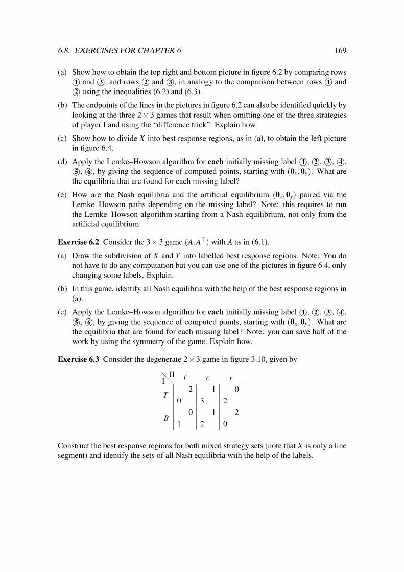
6.8. EXERCISES FOR CHAPTER 6 169
(a) Show how to obtain the top right and bottom picture in figure 6.2 by comparing rows©1 and©3 , and rows©2 and©3 , in analogy to the comparison between rows©1 and©2 using the inequalities (6.2) and (6.3).
(b) The endpoints of the lines in the pictures in figure 6.2 can also be identified quickly bylooking at the three 2×3 games that result when omitting one of the three strategiesof player I and using the “difference trick”. Explain how.
(c) Show how to divide X into best response regions, as in (a), to obtain the left picturein figure 6.4.
(d) Apply the Lemke–Howson algorithm for each initially missing label©1 ,©2 ,©3 ,©4 ,©5 , ©6 , by giving the sequence of computed points, starting with (0x,0y). What arethe equilibria that are found for each missing label?
(e) How are the Nash equilibria and the artificial equilibrium (0x,0y) paired via theLemke–Howson paths depending on the missing label? Note: this requires to runthe Lemke–Howson algorithm starting from a Nash equilibrium, not only from theartificial equilibrium.
Exercise 6.2 Consider the 3×3 game (A,A>) with A as in (6.1).
(a) Draw the subdivision of X and Y into labelled best response regions. Note: You donot have to do any computation but you can use one of the pictures in figure 6.4, onlychanging some labels. Explain.
(b) In this game, identify all Nash equilibria with the help of the best response regions in(a).
(c) Apply the Lemke–Howson algorithm for each initially missing label©1 ,©2 ,©3 ,©4 ,©5 , ©6 , by giving the sequence of computed points, starting with (0x,0y). What arethe equilibria that are found for each missing label? Note: you can save half of thework by using the symmetry of the game. Explain how.
Exercise 6.3 Consider the degenerate 2×3 game in figure 3.10, given by
@@I
II
T
B
l c r
0 3 22 1 0
1 2 00 1 2
Construct the best response regions for both mixed strategy sets (note that X is only a linesegment) and identify the sets of all Nash equilibria with the help of the labels.

170 CHAPTER 6. GEOMETRIC REPRESENTATION OF EQUILIBRIA

Chapter 7
Linear programming and zero-sumgames
This chapter is another extension of the lecture notes “Game Theory Basics” on topicsthat have been first taught in autumn 2010. It comprises a second week of lectures thatpartially replace the old chapter 5 on bargaining, and follows on from section 3.14.
The topic of this chapter is the strong connection between linear programming andfinding equilibria of zero-sum games. Linear programming is the science of solving linearoptimization problems, also called linear programs. It can be applied to zero-sum games,as we explain in this chapter. The central theorem of linear programming is the dualitytheorem (Theorem 7.3). In Section 7.3, we first define linear programs in the standardinequality form. Finding bounds for the objective function motivates the construction ofthe dual linear program, as we show with an example. We then state the weak and strongduality theorems.
In Section 7.4, we show how the strong duality theorem implies the minimax theoremfor zero-sum games.
Section 7.5 is concerned with linear programs in general form where variables may benonnegative or unconstrained, and the linear constraints may be inequalities or equations.The corresponding duality theorem is a very useful tool, and it is worth acquiring practicein using it. We will give several exercises that show its use.
As non-examinable material, we also give a proof of the strong duality theorem, withthe help of Farkas’s Lemma, also known as the theorem of the separating hyperplane.This is done in Section 7.6.
7.1 Learning objectives
After studying this chapter, you should be able to:
• Write down a linear program (LP) in standard inequality form (7.1) and its corre-sponding Tucker diagram (7.4) and understand how to read this diagram to obtain thedual LP (7.3).
171

172 CHAPTER 7. LINEAR PROGRAMMING AND ZERO-SUM GAMES
• State the weak and strong duality theorems.
• Do the same for an LP in general form.
• Apply LP duality as in the exercises.
7.2 Further reading
A good introductory text for linear programming is:
• V. Chvatal (1983), Linear Programming. Freeman, New York.
Shorter, classical texts that give mathematical definitions more directly are:
• G. B. Dantzig (1963), Linear Programming and Extensions. Princeton UniversityPress, Princeton.
• D. Gale (1960), The Theory of Linear Economic Models. McGraw-Hill, New York.
7.3 Linear programs and duality
We use the following notation. For positive integers m,n, the set of m× n matrices isdenoted by Rm×n. An m-vector is an element of Rm. Unless stated otherwise, all vectorsare column vectors, so a vector x in Rm is considered as an m×1 matrix. Its transpose x>is the corresponding row vector in R1×m. The vectors 0 and 1 have all components equalto zero and one, respectively, and have suitable dimension, which may vary with each useof 0 or 1. An inequality like x ≥ 0 holds for all components. The identity matrix, of anydimension, is denoted by I.
A linear optimization problem or linear program (LP) says: optimize (maximize orminimize) a linear objective function subject to linear constraints (inequalities or equali-ties).
The standard inequality form of an LP is given by an m×n matrix A, an m-vector band an n-vector c and says:
maximize c>x
subject to Ax≤ b ,
x≥ 0 .
(7.1)
Thereby, x is the n-vector (x1, . . . ,xn)> of variables. The vector c of coefficients de-termines the objective function. The matrix A and the vector b determine the m linearconstraints, which are here only inequalities. Furthermore, all variables x1, . . . ,xn areconstrained to be nonnegative; this is stated as x ≥ 0 separately from Ax ≤ b becausenonnegative variables are a standard case.
The LP (7.1) states maximization subject to “upper bounds” (inequalities “≤”). Away to remember this is to assume that the components of b and A are positive (they donot have to be), so that these impose actual constraints on x. Clearly, if A has only positiveentries, then Ax≤ b can only be fulfilled for nonnegative x if b≥ 0.

7.3. LINEAR PROGRAMS AND DUALITY 173
In general, the LP (7.1) is called feasible if Ax≤ b and x≥ 0 hold for some x, other-wise infeasible. If c>x can be arbitrarily large for suitable x subject to these constraints,then the LP is called unbounded, otherwise bounded. The LP has an optimal solution onlyif it is feasible and bounded.
Example 7.1 Consider (7.1) with
A =[
3 4 21 1 1
], b =
[72
], c> = [8 10 5 ] ,
which can be stated explicitly as: for x1,x2,x3 ≥ 0 subject to
3x1 + 4x2 +2x3 ≤ 7
x1 + x2 + x3 ≤ 2
maximize 8x1 +10x2 +5x3
(7.2)
The bar is commonly written to separate the objective function from the constraints.
One feasible solution to (7.2) is x1 = 0, x2 = 1, x3 = 1 with objective function value15. Another is x1 = 1, x2 = 1, x3 = 0 with objective function value 18, which is better.(We often choose integers in our examples, but coefficients and variables are allowed toassume any real values.) How do we know when we have an optimal value?
The dual of an LP can be motivated by finding an upper bound to the objective func-tion of the given LP (which is called the primal LP). The dual LP results by readingthe constraint matrix vertically rather than horizontally, exchanging the roles of objectivefunction and right hand side, as follows.
In the example (7.2), we multiply each of the two inequalities by some nonnegativenumber, for example the first inequality by y1 = 1 and the second by y2 = 6, and add theinequalities up, which yields
(3+6)x1 +(4+6)x2 +(2+6)x3 ≤ 7+6 ·2or
9x1 +10x2 +8x3 ≤ 19.
In this inequality, which holds for any feasible solution, all coefficients of the nonnegativevariables x j are at least as large as in the primal objective function, so the right hand side19 is certainly an upper bound for this objective function. In fact, we can obtain an evenbetter bound by multiplying the two primal inequalities by y1 = 2 and y2 = 2, getting
(3 ·2+2)x1 +(4 ·2+2)x2 +(2 ·2+2)x3 ≤ 2 ·7+2 ·2or
8x1 +10x2 +6x3 ≤ 18.
Again, all coefficients are at least as large as in the primal objective function. Thus,it cannot be larger than 18, which was achieved by the above solution x1 = 1, x2 = 1,x3 = 0, which is therefore optimal.
In general, the dual LP for the primal LP (7.1) is obtained as follows:
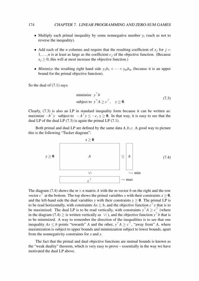
174 CHAPTER 7. LINEAR PROGRAMMING AND ZERO-SUM GAMES
• Multiply each primal inequality by some nonnegative number yi (such as not toreverse the inequality).
• Add each of the n columns and require that the resulting coefficient of x j for j =1, . . . ,n is at least as large as the coefficient c j of the objective function. (Becausex j ≥ 0, this will at most increase the objective function.)
• Minimize the resulting right hand side y1b1 + · · ·+ ymbm (because it is an upperbound for the primal objective function).
So the dual of (7.1) says:
minimize y>b
subject to y>A≥ c>, y≥ 0.(7.3)
Clearly, (7.3) is also an LP in standard inequality form because it can be written as:maximize −b>y subject to −A>y ≤ −c, y ≥ 0. In that way, it is easy to see that thedual LP of the dual LP (7.3) is again the primal LP (7.1).
Both primal and dual LP are defined by the same data A,b,c. A good way to picturethis is the following “Tucker diagram”:
c>
∨
A
x≥ 0
y≥ 0 ≤ b
→ max
↪→ min
(7.4)
The diagram (7.4) shows the m×n matrix A with the m-vector b on the right and the rowvector c> at the bottom. The top shows the primal variables x with their constraints x≥ 0,and the left-hand side the dual variables y with their constraints y ≥ 0. The primal LP isto be read horizontally, with constraints Ax ≤ b, and the objective function c>x that is tobe maximized. The dual LP is to be read vertically, with constraints y>A ≥ c> (wherein the diagram (7.4) ≥ is written vertically as ∨ ), and the objective function y>b that isto be minimized. A way to remember the direction of the inequalities is to see that oneinequality Ax ≤ b points “towards” A and the other, y>A ≥ c>, “away from” A, wheremaximization is subject to upper bounds and minimization subject to lower bounds, apartfrom the nonnegativity constraints for x and y.
The fact that the primal and dual objective functions are mutual bounds is known asthe “weak duality” theorem, which is very easy to prove – essentially in the way we havemotivated the dual LP above.

7.4. THE MINIMAX THEOREM VIA LP DUALITY 175
Theorem 7.2 (Weak LP duality) For a pair x,y of feasible solutions of the primal LP(7.1) and its dual LP (7.3), the objective functions are mutual bounds:
c>x≤ y>b.
If thereby c>x = y>b (equality holds), then these two solutions are optimal for both LPs.
Proof. In general, if u,v,w are vectors of the same dimension, then
u≥ 0, v≤ w ⇒ u>v≤ u>w, (7.5)
because v ≤ w is equivalent to (w− v) ≥ 0 which with u ≥ 0 implies u>(w− v) ≥ 0 andhence u>v≤ u>w; note that this is an inequality between scalars which can also be writtenas v>u≤ w>u.
Feasibility of x for (7.1) and of y for (7.3) means Ax ≤ b, x ≥ 0, y>A ≥ c>, y ≥ 0.Using (7.5), this implies
c>x≤ (y>A)x = y>(Ax)≤ y>b
as claimed.
If c>x∗=(y∗)>b for some primal feasible x∗ and dual feasible y∗, then c>x≤ (y∗)>b =c>x∗ for any primal feasible x, and y>b≥ c>x∗ = (y∗)>b for any dual feasible y, so equal-ity of the objective functions implies optimality.
The following “strong duality” theorem is the central theorem of linear programming.
Theorem 7.3 (Strong LP duality) Whenever both the primal LP (7.1) and its dual LP(7.3) are feasible, they have optimal solutions with equal value of their objective func-tions.
We will prove this theorem in Section 7.6. Its proof is not trivial. In fact, manytheorems in economics have a hidden LP duality so that they can be proved by writingdown a suitable LP and interpreting its dual LP. For that reason, Theorem 7.3 is extremelyuseful. A first, classical application is the proof of the minimax theorem.
7.4 The minimax theorem via LP duality
In this section, we prove the minimax theorem, that is, the existence of an equilibrium fora finite zero-sum game, with the help of Theorem 7.3.
Consider an m× n zero-sum game given by the game matrix A with payoffs ai j for1 ≤ i ≤ m and 1 ≤ j ≤ n to the row player (the maximizer). The problem of finding amin-max strategy for the column player (the minimizer) can be stated as follows: Findprobabilities q1, . . . ,qn and a real number u so that
n
∑j=1
ai jq j ≤ u (1≤ i≤ m) (7.6)

176 CHAPTER 7. LINEAR PROGRAMMING AND ZERO-SUM GAMES
and so that u is minimal. Then the column player does not have to pay more than u for anypure strategy i of the row player, so u is clearly the min-max cost. The problem of findingq1, . . . ,qn and u defines already an LP, except that it is not in the standard inequality formbecause of the equality constraint q1 + · · ·+qn = 1 for the probabilities.
We do obtain an LP with constraints Ax ≤ b and x ≥ 0 with the game matrix A asfollows:
• Assume that all payoffs ai j are positive, if necessary by adding a constant to allpayoffs.
• Then (7.6) implies u > 0 whenever q1, . . . ,qn are probabilities, so that (7.6) is equiv-alent to
n
∑j=1
ai j(q j/u)≤ 1 (1≤ i≤ m). (7.7)
• Consider the LP
maximizen
∑j=1
x j
subject ton
∑j=1
ai jx j ≤ 1 (1≤ i≤ m)
x j ≥ 0 (1≤ j ≤ n).
(7.8)
Then the minimax theorem can be stated as follows.
Theorem 7.4 Consider an m× n zero-sum game with payoffs ai j > 0 to the row player.An optimal solution x∗ to the LP (7.8) with u∗ defined as u∗ = 1/∑n
j=1 x∗j defines a min-max strategy q of the column player by q j = x∗j · u∗ for 1 ≤ j ≤ n. The dual LP of (7.8)is
minimizem
∑i=1
yi
subject tom
∑i=1
yiai j ≥ 1 (1≤ j ≤ n)
yi ≥ 0 (1≤ i≤ m).
(7.9)
Its optimal solution y∗ fulfills u∗ = 1/∑mi=1 y∗i and defines a max-min strategy p of the row
player by pi = y∗i ·u∗ for 1≤ i≤m, so (p,q) is a Nash equilibrium of the game. The valueof the game is u∗.
Proof. The LP (7.8) is feasible with x = 0. Its Tucker diagram is

7.5. GENERAL LP DUALITY 177
1>
∨
A
x≥ 0
y≥ 0 ≤ 1
→ max
↪→ min
(7.10)
which shows that (7.9) is indeed its dual LP. This dual LP is also feasible, for examplewith y1 = max{1/a1 j | 1≤ j≤ n} and y2 = · · ·= ym = 0. By Theorem 7.3, both LPs haveoptimal solutions x∗ and y∗ with equal objective function value v∗ = ∑n
j=1 x∗j = ∑mi=1 y∗i
where v∗ > 0 because y∗ 6= 0 since y = 0 is not feasible for (7.9). Hence, u∗ = 1/v∗ existsas claimed. With q = x · u∗, (7.6) holds with u = u∗. Hence, q is a mixed strategy of thecolumn player who has to pay no more than u∗ against any pure strategy i (and thereforealso against any mixed strategy) of the row player. Similarly, p = y ·u∗ is a mixed strategyof the row player where (7.9) implies
m
∑i=1
piai j ≥ u∗ (1≤ j ≤ n),
that is, against any column j he gets at least payoff u∗. Hence the max-min-value andmin-max-value of the game are both equal to u∗, which is the value of the game, and(p,q) is a Nash equilibrium.
The Tucker diagram (7.10) shows how the zero-sum game matrix A defines an LPwhere the column player chooses the primal variables x and the row player chooses thedual variables y. Optimal primal and dual solutions x∗,y∗ are nonnegative and nonzeroand can therefore be normalized, by multiplication with a constant u∗ (the inverse ofthe optimal value of both objective functions), so that x∗,y∗ becomes a pair of mixedstrategies q, p, where q is a min-max strategy and p is a max-min strategy. In (7.10),the vectors 1 and 1> define the primal and dual “right-hand side”. After normalizing themixed strategies, each component 1 of these vectors becomes the min-max cost u∗ in eachrow and max-min payoff u∗ in each column. Hence, these 1’s in (7.10) represent this costand payoff before normalization. It is important that A has only positive entries in orderto guarantee that the game has a positive value, that is, u∗ > 0, so that the normalizationis possible.
7.5 General LP duality
An LP in standard inequality form is not always the most convenient way to use theduality theorem, which holds in a more general setting. In this section, we consider thegeneral form of an LP that allows for linear equalities as constraints (in addition to linearinequalities), and for variables that are unrestricted in sign (in addition to the standard

178 CHAPTER 7. LINEAR PROGRAMMING AND ZERO-SUM GAMES
case of nonnegative variables). These cases are closely related with respect to the dualityproperty. As we will see, a primal equality constraint corresponds to a dual variable thatis unrestricted in sign, and a primal variable that is unrestricted in sign gives rise to a dualconstraint that is an equality. The other case, which we have already seen, is a primalinequality that corresponds to a dual variable that is nonnegative, or a primal nonnegativevariable where the corresponding dual constraint is an inequality.
In the standard in LP in inequality form (7.1), the constraint x ≥ 0 looks somewhatredundant since the nonnegativity of x can easily be made part of Ax ≤ b by including inthose inequalities n additional inequalities −x j ≤ 0 for 1≤ j ≤ n. By omitting nonnega-tivity of x, one obtains an LP with unconstrained variables x, given by
maximize c>x
subject to Ax≤ b.(7.11)
With (7.11) as the primal LP, we can again multiply any of the inequalities in Ax≤ b witha variable yi, with the aim of finding an upper bound to the primal objective function c>x.The inequality is preserved when yi is nonnegative, but in order to obtain an upper boundwe have to require that y>A = c> because the sign of any component of x is not known.That, is the dual to (7.11) is
minimize y>b
subject to y>A = c>, y≥ 0.(7.12)
Weak duality applied to the pair of prima and dual LPs (7.11) and (7.12) states that forfeasible solutions x and y the corresponding objective functions are mutual bounds, thatis (including proof)
c>x = y>Ax≤ y>b. (7.13)
Another case is an LP with nonnegative variables and equality constraints, which isoften called an LP in equality form:
maximize c>x
subject to Ax = b ,
x≥ 0 .
(7.14)
In the corresponding dual LP, each constraint in Ax = b is again multiplied with a dualvariable yi. However, because the constraint is an equality, the variable yi can be unre-stricted in sign. The dual constraints are inequalities because the primal objective functionhas nonnegative variables x j. That is, the dual LP to (7.14) is
minimize y>b
subject to y>A≥ c>.(7.15)
The weak duality theorem uses that for feasible solutions x and y to (7.14) and (7.15) wehave x≥ 0 and y>A− c> ≥ 0 and thus
c>x≤ y>Ax = y>b. (7.16)

7.5. GENERAL LP DUALITY 179
These two cases, of a primal LP (7.11) with unrestricted variables and a correspond-ing dual LP (7.12) with equality constraints, and of a primal LP (7.14) with nonnegativevariables and (7.15) with equality constraints, and of a corresponding dual LP with unre-stricted variables, show that as before the dual of the dual is the primal.
Any LP in inequality form (7.1) can be converted to equality form by introducing aslack variable zi for each constraint:
maximize c>x
subject to Ax+ z = b ,
x ≥ 0
z≥ 0 .
(7.17)
This amounts to extending the constraint matrix A to the right by an identity matrix andby adding coefficients 0 in the objective function for the slack variables.
Note: Converting the inequality form (7.1) to equality form (7.17) defines a new dualLP with unrestricted variables y1, . . . ,ym, but the former inequalities yi ≥ 0 reappear nowexplicitly via the identity matrix and objective function zeros introduced with the slackvariables, as shown in the following Tucker diagram.
z≥ 0
∨
11
. . .
1
0 0 · · · 0c>∨
A
x≥ 0
y ∈ R = b
An LP in general form has inequalities and equalities as constraints, as well as non-negative and unrestricted variables. In the dual LP, the inequalities correspond to non-negative variables and the equalities correspond to unrestricted variables and vice versa.The full definition of an LP in general form is as follows. Let M and N be finite sets(whose elements denote rows and columns, respectively), I ⊆M, J ⊆ N, A ∈ RM×N (thatis, A is a matrix with entries ai j for i ∈M and j ∈ N), b ∈ RM, c ∈ RN . We first draw theTucker diagram, shown in Figure 7.1. The big boxes contain the respective parts of theconstraint matrix A, the vertical boxes on the right the parts of the right hand side b, andthe horizontal box at the bottom the parts of the primal objective function c>.
Here the indices in I denote primal inequalities and corresponding nonnegative dualvariables, whereas those in M− I denote primal equality constraints and correspondingunconstrained dual variables. Analogously, the indices in J denote primal variables thatare nonnegative and corresponding dual inequalities, whereas the indices in N − J de-note unconstrained primal variables and corresponding unconstrained dual equality con-straints. Figure 7.1 is drawn as if the elements of I and J are listed first in the sets M andN, respectively, but the order of the indices in M and N does not matter.
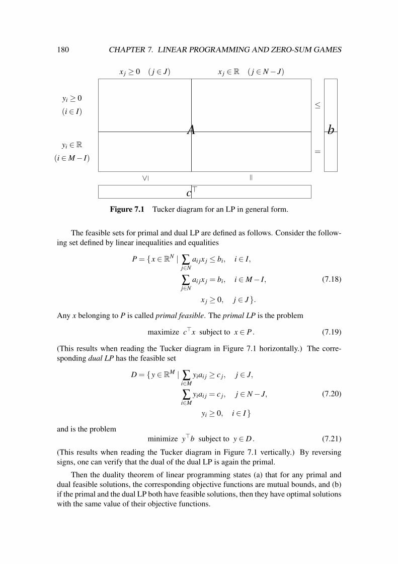
180 CHAPTER 7. LINEAR PROGRAMMING AND ZERO-SUM GAMES
c>
A byi ∈ R
(i ∈M− I)=
yi ≥ 0
(i ∈ I)≤
∨
x j ≥ 0 ( j ∈ J) x j ∈ R ( j ∈ N− J)
Figure 7.1 Tucker diagram for an LP in general form.
The feasible sets for primal and dual LP are defined as follows. Consider the follow-ing set defined by linear inequalities and equalities
P = {x ∈ RN | ∑j∈N
ai jx j ≤ bi, i ∈ I,
∑j∈N
ai jx j = bi, i ∈M− I,
x j ≥ 0, j ∈ J }.
(7.18)
Any x belonging to P is called primal feasible. The primal LP is the problem
maximize c>x subject to x ∈ P . (7.19)
(This results when reading the Tucker diagram in Figure 7.1 horizontally.) The corre-sponding dual LP has the feasible set
D = {y ∈ RM | ∑i∈M
yiai j ≥ c j, j ∈ J,
∑i∈M
yiai j = c j, j ∈ N− J,
yi ≥ 0, i ∈ I }
(7.20)
and is the problemminimize y>b subject to y ∈ D . (7.21)
(This results when reading the Tucker diagram in Figure 7.1 vertically.) By reversingsigns, one can verify that the dual of the dual LP is again the primal.
Then the duality theorem of linear programming states (a) that for any primal anddual feasible solutions, the corresponding objective functions are mutual bounds, and (b)if the primal and the dual LP both have feasible solutions, then they have optimal solutionswith the same value of their objective functions.
7.6. THE LEMMA OF FARKAS AND PROOF OF STRONG LP DUALITY∗ 181
Theorem 7.5 (General LP duality) Consider the primal-dual pair of LPs (7.19), (7.21).Then(a) (Weak duality.) c>x≤ y>b for all x ∈ P and y ∈ D.(b) (Strong duality.) If P 6= /0 and D 6= /0 then c>x = y>b for some x ∈ P and y ∈ D.
Theorem 7.5 can be proved with the help of Theorem 7.3 by representing an equationas two inequalities in opposite directions, and an unrestricted variable as the difference oftwo nonnegative variables. The details are omitted for the moment.
7.6 The Lemma of Farkas and proof of strong LP duality∗
In this section, we state and prove Farkas’s Lemma, also know as the theorem of theseparating hyperplane, and use it to prove Theorem 7.3.
The Lemma of Farkas is concerned with the question of finding a nonnegative so-lution x to a system Ax = b of linear equations. If A = [A1 · · ·An], this means that b isa nonnegative linear combination A1x1 + · · ·+ Anxn of the columns of A. We first ob-serve that such linear combinations can always be obtained by taking suitable linearlyindependent columns of A.
Lemma 7.6 Let A = [A1 · · ·An] ∈ Rm×n, let v ∈ Rm, and let
C = {Ax | x ∈ Rn, x≥ 0}. (7.22)
Then if v ∈ C, there is a set J ⊆ {1, . . . ,n} so that the vectors A j for j ∈ J are linearlyindependent, and unique positive reals u j for j ∈ J so that
∑j∈J
A ju j = v. (7.23)
Proof. Because v ∈C, we have Au = v for some u≥ 0, so that (7.23) holds with J = { j |u j > 0}. If the vectors A j for j ∈ J are linearly independent (in which case we simply callJ independent), we are done. Otherwise, we change the coefficients u j by keeping themnonnegative but so that at least one of them becomes zero, which gives a smaller set J.
Suppose J is not independent, that is, there are scalars x j for j ∈ J, not all zero, sothat
∑j∈J
A jx j = 0,
where we can assume that the set S = { j ∈ J | x j > 0} is not empty (otherwise replace xby −x). Then
∑j∈J
A j(u j−λx j) = v
for any λ . We choose the largest λ so that u j−λx j ≥ 0 for all j ∈ J. If x j ≤ 0 this imposesno constraint on λ , but for x j > 0 (that is, j ∈ S) this means u j/x j ≥ λ , so the largest λfulfilling all these constraints is given by
λ = min{u j
x j| j ∈ S}=:
u j∗
x j∗(7.24)

182 CHAPTER 7. LINEAR PROGRAMMING AND ZERO-SUM GAMES
which implies u j∗−λx j∗ = 0 so that we can remove any j∗ that achieves the minimum in(7.24) from J. By replacing u j with u j−λx j, we thus obtain a smaller set J to representv as in (7.23). By continuing in this manner, we eventually obtain an independent set J asclaimed (if v = 0, then J is the empty set). Because the vectors A j for j ∈ J are linearlyindependent, the scalars u j for j ∈ J are unique.
The set C in (7.22) of nonnegative linear combinations of the column vectors of Ais also called the cone generated by these vectors. Figure 7.2(a) gives an example withA ∈ R2×4 and a vector b ∈ R2 that is not in the cone C generated by A1,A2,A3,A4.
C
b0
1
A4
A3
A2
A
(a)
cyH
(b)
0
A1
A4
A3
A2
C
b
Figure 7.2 (a) vectors A1,A2,A3,A4, the cone C generated by them, and a vector b notin C; (b) a separating hyperplane H for b with normal vector y = c−b.
For the same vectors, Figure 7.2(b) shows a vector y with the following properties:
• y>A j ≥ 0 for all j, for 1≤ j ≤ n, and
• y>b < 0.
The set H = {z ∈ Rm | y>z = 0} is called a separating hyperplane with normal vectory because all vectors A j are on one side of H (they fulfill y>A j ≥ 0, which includes thecase y>A j = 0 where A j belongs to H, like A2 in Figure 7.2(b)), whereas b is strictlyon the other side of H because y>b < 0. Farkas’s Lemma asserts that such a separatinghyperplane exists for any b that does not belong to C.
Lemma 7.7 (Farkas) Let A ∈ Rm×n and b ∈ Rm. Then either
(a) ∃x ∈ Rn : x≥ 0, Ax = b, or
(b) ∃y ∈ Rm : y>A≥ 0, y>b < 0.
In Lemma 7.7, it is clear that (a) and (b) cannot both hold because if (a) holds, theny>A≥ 0 implies y>b = y>(Ax) = (y>A)x≥ 0.
If (a) is false, that is, b does not belong to the cone C in (7.22), then y can be con-structed by the following intuitive geometric argument: Take the vector c in C that isclosest to b (see Figure 7.2(b)), and let y = c− b. We will show that y fulfills the condi-tions in (b).

7.6. THE LEMMA OF FARKAS AND PROOF OF STRONG LP DUALITY∗ 183
Apart from this geometric argument, an important part of the proof is to show that thecone C is topologically closed, that is, it contains any point nearby. Otherwise, b could bea point near C but not in C which would mean that the distance ||c−b|| for any c in C canbe arbitrarily small, where ||z|| denotes the Euclidean norm, ||z|| =
√z>z. In that case,
one could not define y as described. We first show that C is closed as a separate property.
Lemma 7.8 For an m×n matrix A = [A1 · · ·An], the cone C in (7.22) is a closed set.
Proof. Let z be a point in Rm near C, that is, for all ε > 0 there is a v in C so that||v− z|| < ε . Consider a sequence v(k) (for k = 1,2, . . .) of elements of C that convergesto z. By Lemma 7.6, for each k there exist a subset J(k) of {1, . . . ,n} and unique positivereal numbers u(k)
j for j ∈ J(k) so that the columns A j for j ∈ J(k) are linearly independentand
v(k) = ∑j∈J(k)
A ju(k)j .
There are only finitely many different sets J(k), so there is a set J that appears infinitelyoften among them; we consider the subsequence of the vectors v(k) that use this set, thatis,
v(k) = ∑j∈J
A ju(k)j = AJu(k)
J (7.25)
where AJ is the matrix with columns A j for j ∈ J and u(k)J is the vector with components
u(k)j for j ∈ J. Now, u(k)
J in (7.25) is a continuous function of v(k): In order to see this,consider a set I of |J| linearly independent rows of AJ , let AIJ be the square submatrix of AJ
with these rows and let v(k)I be the subvector of v(k) with these rows, so that u(k)
J = A−1IJ v(k)
I
in (7.25). Hence, as v(k) converges to z, the |J|-vector u(k)J converges to some u∗J with
z = AJu∗J , where u(k)J > 0 implies u∗J ≥ 0, which shows that z ∈C.
Remark 7.9 In Lemma 7.8, it is important that C is the cone generated by a finite setA1, . . . ,An of vectors. The cone generated from an infinite set may not be closed. Forexample, let C be the set of nonnegative linear combinations of the (row) vectors (n,1) inR2, for n = 0,1,2, . . .. Then (1,0) is a vector near C that does not belong to C.
⇒ Prove Remark 7.9, by giving an exact description of C.
⇒ Show that Farkas’s Lemma 7.10 below implies that the cone C in (7.22) is an in-tersection of half-spaces, that is, of sets of the form {v ∈ Rm | a>v ≤ a0} for somea ∈ Rm and a0 ∈ R, which implies that C is closed. However, note that the proof ofthe lemma uses that C is closed, so this has to be shown first.
Proof of Lemma 7.7. Let A = [A1 · · ·An] and C as in (7.22). Assume that (a) is false, thatis, b 6∈C; we have to prove that (b) holds. Choose c ∈C so that ||c−b|| is minimal. Thisminimum exists because C is closed by Lemma 7.8. Then ||c−b||> 0 because b 6∈C, andthus ||c−b||2 = (c−b)>(c−b) > 0, that is,
(c−b)>c > (c−b)>b . (7.26)
184 CHAPTER 7. LINEAR PROGRAMMING AND ZERO-SUM GAMES
Let y = c−b. We show that for all d in C
(c−b)>d ≥ (c−b)>c . (7.27)
If (7.27) was false, then(c−b)>(d− c) < 0 (7.28)
for some d in C. Consider the convex combination of d and c given by dε = c+ε(d−c) =(1− ε)c+ εd which belongs to C, which is clearly a convex set. Then
||dε −b||2 = ||c−b||2 + ε(
2(c−b)>(d− c)+ ε||d− c||2)
which by (7.28) is less than ||c− b||2 for sufficiently small positive ε , which contradictsthe minimality of ||c−b||2 for c ∈C. So (7.27) holds.
In particular, for d = A j + c we have y>A j ≥ 0, for any 1≤ j ≤ n, that is, y>A≥ 0.
Equations (7.27) and (7.26) imply (c−b)>d > (c−b)>b for all d ∈C. For d = 0 thisshows 0 > y>b.
Lemma 7.7 is concerned with finding nonnegative solutions x to a system of equationsAx = b. We will use a closely related “inequality form” of this lemma that concernsnonnegative solutions x to a system of inequalities Ax≤ b.
Lemma 7.10 (Farkas with inequalities) Let A ∈ Rm×n and b ∈ Rm. Then either
(a) ∃x ∈ Rn : x≥ 0, Ax≤ b, or
(b) ∃y ∈ Rm : y≥ 0, y>A≥ 0, y>b < 0.
Proof. Clearly, there is a vector x so that Ax≤ b and x≥ 0 if and only if there are x ∈ Rn
and s ∈ Rm withAx+ s = b, x≥ 0, s≥ 0. (7.29)
The system (7.29) is a system of equations as in Lemma 7.7 with the matrix [A I], whereI is the m×m identity matrix, instead of A, and vector (x,s)> instead of x. The conditiony>[A I]≥ 0 in Lemma 7.7(b) is then simply y≥ 0, y>A≥ 0 as stated here in (b).
The conversion of inequalities Ax≤ b to a system of equations by means of nonneg-ative “slack variables” as in (7.29) is a standard trick in linear programming that we haveseen before.
We can now prove the strong duality theorem.
Proof of Theorem 7.3. We assume that (7.1) and (7.3) are feasible, and want to show thatthere are feasible x and y so that c>x ≥ y>b, which by Theorem 7.2 implies c>x = y>b.Suppose, to the contrary, that there are x,y so that
x≥ 0, Ax≤ b, y≥ 0, yT A≥ c> (7.30)

7.7. EXERCISES FOR CHAPTER 7 185
but no solution x,y to the system of inequalities
−A>y≤ − c
Ax ≤ b
−c>x +b>y≤ 0
(7.31)
and x,y≥ 0. By Lemma 7.10, this means there are u ∈ Rm, v ∈ Rn, and t ∈ R so that
u≥ 0, v≥ 0, v>A− tc> ≥ 0, t ≥ 0, u>(−A>)+ tb> ≥ 0, (7.32)
but−u>c+ v>b < 0. (7.33)
We derive a contradiction as follows: If t = 0, this means v>A≥ 0, u>A> ≤ 0, which with(7.31), using (7.30), implies
v>b≥ v>Ax≥ 0≥ u>A>y≥ u>c
in contradiction to (7.33).
If t > 0, then u and v are essentially primal and dual feasible solutions that violateweak LP duality, because then by (7.32) bt ≥ Au and v>A≥ tc> and therefore
v>bt ≥ v>Au≥ tc>u
which after division by t gives v>b≥ c>u, again contradicting (7.33).
So if the first two sets of inequalities in (7.31) have a solution x,y ≥ 0, then there isalso a solution that fulfills the last inequality, as claimed by strong LP duality.
7.7 Exercises for chapter 7
Exercise 7.1 As in Section 7.4, consider a zero-sum game with an m× n matrix A ofpayoffs to player 1 (the maximizing row player). The minimax theorem was proved withthe help of LP duality by converting the constraints in (7.6) to (7.7) and arriving at an LP(7.8). The assumption was that A has positive entries. Instead, use the duality theorem forgeneral LPs by considering directly the inequalities in (7.6) with an unconstrained dualvariable u, and the additional equality constraint that q1, . . . ,qn are probabilities, to provethe minimax theorem. Why do you no longer need any sign restrictions about the entriesof the matrix A?
Exercise 7.2 Consider an m×n game with payoffs ai j to player I. A mixed strategy p ofplayer I is said to dominate a pure strategy i if the expected payoff to player I resultingfrom p is always larger than the payoff resulting from i no matter which pure strategy j ischosen by player II. (Note that p may be a pure strategy in the sense that this pure strategyis chosen with probability 1 by p.) That is, for all j = 1, . . . ,n we have
m
∑k=1
pkak j > ai j .

186 CHAPTER 7. LINEAR PROGRAMMING AND ZERO-SUM GAMES
Moreover, here we can assume pi = 0 because pi = 1 is clearly not possible, and then pkfor k 6= i can be replaced by pk/∑m
l=1, l 6=i pl and pi set to zero.
(a) The following is the matrix of payoffs to player I in a 3×2 game:
A =
6 00 62 2
.
Show that the bottom row of player I is dominated by a mixed strategy.
(b) Consider the following statements and argue that (1) implies (2):
(1) Strategy i of player I is a best response to a suitable mixed strategy q of player II.
(2) Strategy i of player I is not dominated by a mixed strategy.
(c) The following is the matrix of payoffs to player I in a 3×2 game:
A =
6 00 64 4
.
Show that the bottom row of player I is not dominated by a mixed strategy.
(d) Show, using linear programming duality, that in (b) also statement (2) implies state-ment (1), so that the two statements are in fact equivalent. Since it takes some practiceto do this, here are fairly detailed instructions: Write down condition (1) as a primalLP, with the following components: a linear equation that states that row i of A hasexpected payoff u against a mixed strategy q of player II; next, inequalities statingthat all other rows k have smaller payoff than u, by introducing a variable that de-notes the difference – that variable is then maximized in the linear program; andfinally, that the variables that describe the mixed strategy q of player II are indeeda probability distribution. Once you have done this and have written these equali-ties and inequalities in a Tucker diagram, read that diagram vertically to obtain thedual linear program. The dual variables should then give you the answer (a statementabout mixed strategies p for player I in this case). All you have to do is to suitablyinterpret the fact that the dual program has the same optimal objective function valueas the primal program.