game theory: distributed selfish load balancing on networks · 2015-06-15 · 2 game theory:...
TRANSCRIPT

Faculty of ScienceDepartment of Mathematics
Game Theory: Distributed Selfish LoadBalancing on Networks
Bachelor Thesis I
Filip Moons
Promotor: Prof. Dr. Ann Nowe
January 2013

i
Abstract for non-mathematicians
Explaining the subject of my Bachelor thesis to those who do not study either Math-ematics or Computer Science isn’t an easy task, but I can give an idea of the problemstudied by giving an example. Imagine, for example, that there are only two roads fromParis to Brussels: road A & road B. If you take road A you’ll always drive 5 hours, inde-pendent from the usage of road A by other drivers (agents is the more game theoreticalword). If you take road B, the time you need depends of the number of other agentsusing road B: you’ll drive 5 x
100 hours, with x the number of agents, but also on this roadthe maximum time spend is 5 hours, so mathematically that becomes min(5, 5 x
100 ) hours.Because every agent acts selfish and rational, the result under this circumstances and withonly this information will be that every agent will take at any time road B: with road Athey drive always 5 hours, with road B there is a chance to get to Brussels in less time.But consider now the following situation: exact 100 agents decide at the same time togo to Brussels, that means that all of them will take road B and so everyone will drive5 hours. It would be much better that 50 agents would take road A (and thus drive 5hours) and the other 50 take road B (and drive 5 50
100 = 2.5 hours), that would reduce theaverage time to 3.75 hours! This kind of problems where the selfishness of agents reducethe power (load) of a general system take place in a wide range of real life problems: notonly in traffic, but also in economics, politics and, that’s more my interest, also in Com-puter Science: in a distributed system computers interact on a selfish base because thereisn’t a central computer that organizes the network. It’s extremely interesting to studywhich solutions and/or which information these kind of agents (computers) need to knowor to reduce their selfishness and reach the optimal power of the distributed network.
CONTENTS ii
Contents
1 Introduction 11.1 Why we need Game Theory . . . . . . . . . . . . . . . . . . . . . . . . . . . . 1
2 Game Theory: Introducing Load Balancing Games 12.1 Strategic games . . . . . . . . . . . . . . . . . . . . . . . . . . . . . . . . . . . 1
2.1.1 Definition . . . . . . . . . . . . . . . . . . . . . . . . . . . . . . . . . . 12.1.2 Mixed and pure strategies . . . . . . . . . . . . . . . . . . . . . . . . . 22.1.3 Nash Equilibra . . . . . . . . . . . . . . . . . . . . . . . . . . . . . . . 32.1.4 Theorem of Nash . . . . . . . . . . . . . . . . . . . . . . . . . . . . . . 3
2.2 Congestion games . . . . . . . . . . . . . . . . . . . . . . . . . . . . . . . . . . 52.2.1 Definition . . . . . . . . . . . . . . . . . . . . . . . . . . . . . . . . . . 52.2.2 The existence of a pure Nash equilbrum . . . . . . . . . . . . . . . . . 6
2.3 Load balancing games . . . . . . . . . . . . . . . . . . . . . . . . . . . . . . . 82.3.1 Definition . . . . . . . . . . . . . . . . . . . . . . . . . . . . . . . . . . 82.3.2 Payoffs and makespan for linear cost functions . . . . . . . . . . . . . 8
Pure strategies . . . . . . . . . . . . . . . . . . . . . . . . . . . . . . . 8Mixed strategies . . . . . . . . . . . . . . . . . . . . . . . . . . . . . . 9
2.3.3 An example with linear costs . . . . . . . . . . . . . . . . . . . . . . . 10
3 The Price of Anarchy 113.1 Definition . . . . . . . . . . . . . . . . . . . . . . . . . . . . . . . . . . . . . . 113.2 Bachmann-Landau notations . . . . . . . . . . . . . . . . . . . . . . . . . . . 12
3.2.1 Bigh Oh, Big Omega & Big Theta . . . . . . . . . . . . . . . . . . . . 123.2.2 Small Oh, Small Omega & Small Theta . . . . . . . . . . . . . . . . . 133.2.3 Asymptotical Equality . . . . . . . . . . . . . . . . . . . . . . . . . . . 13
3.3 PoA in Pure Nash Equilibria . . . . . . . . . . . . . . . . . . . . . . . . . . . 133.3.1 Identical Machines . . . . . . . . . . . . . . . . . . . . . . . . . . . . . 133.3.2 Uniformly Related Machines . . . . . . . . . . . . . . . . . . . . . . . 14
3.4 PoA in Mixed Nash Equilibria . . . . . . . . . . . . . . . . . . . . . . . . . . 183.4.1 Identical Machines . . . . . . . . . . . . . . . . . . . . . . . . . . . . . 183.4.2 Uniformly Related Machines . . . . . . . . . . . . . . . . . . . . . . . 20
3.5 Summary . . . . . . . . . . . . . . . . . . . . . . . . . . . . . . . . . . . . . . 243.6 PoA in Load Balancing Games with non-linear cost functions . . . . . . . . . 24
4 Coordinations Mechanisms 244.1 Policies . . . . . . . . . . . . . . . . . . . . . . . . . . . . . . . . . . . . . . . 244.2 Taxation . . . . . . . . . . . . . . . . . . . . . . . . . . . . . . . . . . . . . . . 25

1 INTRODUCTION 1
1 Introduction
Whenever a set of tasks should be executed on a set of resources, the problem of load balancingevidently arouses. We need to balance the load among the resources in order to exploit theavailable resources efficiently and fair.
1.1 Why we need Game Theory
One of the most fundamental load balancing problems is makespan scheduling on uniformlyrelated machines. This problem is defined by m machines with speeds s1, ...sm and n taskswith weights w1, ..., wn. Let [n] = 1, ..., n be the set of tasks and [m] the set of machines.Now, the problem is to find an assignment function A : [n]→ [m] of the tasks to the machinesthat is as balanced as possible. The load of machine j ∈ [m] under A is defined as:
`j =∑i∈[n]j=A(i)
wisj
The makespan is defined asmaxj∈[m]
(`j)
Now, of course, the objective is to minimize the makespan. When there is a centralmachine, it ins’t that hard to design algorithms that compute a mapping A that minimizesthe makespan. Suppose, however, that there is not a central machine that can enforce anefficient mapping of the tasks to the machines (e.g. in P2P Networks). This naturally leadsto the following game theoretic setting in which we will be able to analyze what happens tothe makespan if there is no global authority but selfish agents aiming at maximizing theirindividual benefit decide about the assignment of tasks. To understand the problem and it’ssolution, we first give the most important game theoretical results you’ll need.
2 Game Theory: Introducing Load Balancing Games
Important note: This section doesn’t aim to give the reader an introduction in Game Theory.Instead, it gives only the relevant results that the reader must know for understanding therest of this paper.
2.1 Strategic games
2.1.1 Definition
Definition 2.1. [JOARU1994] A strategic game 〈N, (Ai),i〉 consists of:
• a finite set N (the set of players),
• for each player i ∈ N a nonempty set Ai (the set of actions available to player i),
• for each player i ∈ N a preference relation i on A = ×j∈NAj (the preference rela-tion of player i).
2 GAME THEORY: INTRODUCING LOAD BALANCING GAMES 2
Remark 2.2. Under a wide range of circumstances the preference relation i of player i ina strategic game can be represented by a payoff function ui : A → R, in the sense thatui(a) ≥ ui(b) whenever a i b. Sometimes this function is also called a utility function. Astrategic game is then often denoted as G = 〈N, (Ai), (ui)〉. In this paper, we assume thatevery strategic game has a payoff function, because the more general case is irrelevant for thesubject studied.
2.1.2 Mixed and pure strategies
A pure strategy provides a complete definition of how a player will play a game. In particular,it determines the action a player will make for any situation he or she could face. Mathemat-ically, an element a = (a1, ..., an) ∈ A is called pure strategy profile. The components ai of acontain an action for each player at any stage of the game.
A mixed strategy is an assignment of a probability to each action that is available tothe player. This allows for a player to randomly select a pure strategy. Since probabilitiesare continuous, there are infinitely many mixed strategies available to a player, even if theirstrategy set is finite.
Of course, one can regard a pure strategy as a degenerated case of a mixed strategy, inwhich that particular pure strategy is selected with probability 1 and every other strategywith probability 0.
Let in a mixed strategy, αi(aj) (with aj ∈ Ai) denote the probability that player i chooseaction j, thus: αi(aj) = P[Ai = aj ]. A mixed strategy profile
α = (αi)i∈N
specifies the probabilities for all players for all their possible actions. The probability ofobtaining a specific pure strategy profile a = (a1, ..., an) is:
P[α = a] =∏i∈N
αi(ai)
We can now define the expected payoff for player i under a mixed strategy profile α:
Ui(α) =∑a∈A
∏j∈N
αj(aj)
ui(a)
Or, by using the properties of the (discrete) expected value (we iterate over the pure strategyprofiles a ∈ A)1:
Ui(α) = E[ui(a)]
The set of all mixed strategy profiles in a strategic game for a specific player i is denotedas ∆(Ai). Note that (αi(a1), ..., αi(ak), ...) with the aj ’s the pure actions of player i (thusaj ∈ Ai) are the (vector)elements in ∆(Ai). The set of all mixed strategy profiles in a strategicgame is denoted as ∆(A) and is defined as: ∆(A) = ∆(A1)× ...×∆(An) .
1This notation is a little bit ambiguous, because in advanced game theory, also the payoff function may havea distribution. The reader must keep in mind that in this paper, payoff functions do not have a distribution.
2 GAME THEORY: INTRODUCING LOAD BALANCING GAMES 3
2.1.3 Nash Equilibra
One of the most fundamental concepts in game theory is that of Nash equilibrum. This notioncaptures a steady state of the play of a strategic game in which no player can improve hiscost by unilaterally changing his strategy. Of course, we distinguish pure and mixed NashEquilibra.
Definition 2.3. (Pure Nash Equilibrum) [THAR2011] A pure strategy profile a∗ ∈ A is apure Nash Equilibrum if for each player i ∈ N :
ui(a∗−i, a∗i )) ≥ ui(a∗−i, ai) ∀ai ∈ Ai
Definition 2.4. (Mixed Nash Equilibrum)[SUR2004] A mixed strategy profile α∗ is a mixedNash Equilibrum if for each player i ∈ N :
Ui(α∗−i, α∗i )) ≥ Ui(α∗−i, αi) ∀αi
Remark 2.5. The notation (a∗−i, ai) for a pure strategy profile a∗ is a slight abuse of notationthat is quite common in Game Theory, meaning that a∗i ∈ Ai and Sa−i ∈ A1 × ... × Ai−1 ×Ai+1... × An. The same holds for the mixed strategy profiles. It’s important to realize thatplayers have no exact order in a strategy profile, so they can always be re-ordered.
Although there is not enough space to give a deep explanation of the concept of a Nashequilibrum, it’s important to know that a Nash equilibrum is not necessary an optimal solutionof a game. It’s only a profile in which no player will benefit from changing his strategy onit’s own.
2.1.4 Theorem of Nash
Now we have defined the concept of Nash Equilibrum, we can look at one of the most fun-damental theorems in Game Theory: the Theorem of Nash. This theorem states that everyfinite strategic game has at least one mixed Nash Equilibrum.
Nash proved his theorem in 1950 by using the Brouwer fixed point theorem. Later on, a loteasier version of the proof is found by using the Kakutani’s fixed point theorem. However, the(one dimensional version of) the Brouwer fixed point theorem is much more familiar becauseit’s proved in almost every intermediate Analysis course. Therefore, we will give the originalproof of Nash.
Definition 2.6. (Fixed point)[COL2011] Let X be a set and f : X → X a function. A pointx ∈ X is called a fixed point of f if f(x) = x.
Property 2.7. (One dimensional version Brouwer fixed point theorem) [MEU2011] Everycontinuous function
f : [a, b]→ [a, b]has a fixed point.
Proof. As the codomain of f is [a, b] it follows that the image of f is a subset of [a, b]. Thusf(a) ≥ a and f(b) ≤ b. Consider the function
g : [a, b]→ R : x 7→ f(x)− x.
Then is g also continuous and g(a) ≥ 0 and g(b) ≤ 0. By the theorem of Bolzano (see[MEU2011]): ∃c ∈ [a, b] : g(c) = 0, but this means that f(c) = c.
2 GAME THEORY: INTRODUCING LOAD BALANCING GAMES 4
The previous result is a very easy case of the Brouwer fixed point theorem. Proving thegeneral theorem (see below) is very hard and falls behind the scope of this paper.Lemma 2.8. (Brouwer fixed point theorem) Let X be a non-empty, compact and convex set.If f : X → X is continuous, then there must exist x ∈ X such that f(x) = x.Theorem 2.9. (Theorem of Nash) Every finite strategic game has a mixed Nash equilibrum.Proof. For every player i, let the set of actions Ai be a1, ..., am. For 1 ≤ i ≤ n. Let α bea mixed strategy profile of the the game and define gij(α) to be the gain for player i formswitching to his (pure) action aj ,:
gij(α) = maxUi(α−i, aj)− Ui(α), 0We can now define a map between mixed strategies of player i, y : ∆(Ai)→ ∆(Ai) by
yij(α) = αi(aj) + gij(α)1 +
∑mj=1 gij(α)
We now make two observations about this mapping:
• For every player i and his action aj , the mapping gij(α) is continuous. This is due tothe fact that Ui(α) is obviously continuous (it consists of the sum of products betweena probability function and the continuous ui), making gij(α) and consequently yij(α)continuous.
• For every player i, the vector (yij(α))mj=1 is a distribution. This is due to the fact thatthe denominator of yij(α) is a normalization constant for any given i.
• Remember that ∆(Ai) has (vector)elements of the form (αi(a1), ..., αi(ak), ...). Be-cause the given strategic game is finite, we can identify ∆(Ai) with the set of vectors(αi(a1), ..., αi(ak)), for which αi(aj) ≥ 0 ∀j and
∑kj=1 αi(aj) = 1. We now proof that
the set ∆(Ai) satisfies the conditions for the Brouwer fixed point theorem:
– The set ∆(Ai) is non-empty by definition of a strategic game.– To proof that the set ∆(Ai) is convex, take ~x = (αxi (a1), ..., αxi (ak)) and ~y =
(αyi (a1), ..., αyi (ak)) then ~z = θ~x+ (1− θ)~y for some θ ∈ [0, 1] is in ∆(Ai) because~z is also a mixed strategy for player i (the sum of the components of ~z is 1).
– The compactness in Rk can be shown by proving that the set is closed and bounded.The set is bounded because 0 ≤ αi(aj) ≤ 1. To proof closeness in Rk, we’ll proofthat the limit of every convergent sequence in ∆(Ai) is an element of ∆(Ai). Con-sider a convergent sequence in ∆(Ai) : ((αni (a1), ..., αni (ak))n → (α∗i (a1), ..., α∗i (ak)).Remember that a convergent sequence of vectors converges componentwise andthat the addition is a continuous function, so:
k∑j=1
α∗i (aj) =k∑j=1
limn→∞
αni (aj)
= limn→∞
k∑j=1
αni (aj)
= limn→∞
1= 1
2 GAME THEORY: INTRODUCING LOAD BALANCING GAMES 5
this means that (α∗i (a1), ..., α∗i (ak)) is also a mixed strategy for player i, but bydefinition of ∆(Ai), this limit belongs to ∆(Ai).
Therefore y fulfills the conditions of Brouwer’s Fixed Point Theorem. Using the theorem,we conclude that there is a fixed point α∗ for y. This point satisfies
α∗i (aj) = α∗i (aj) + gij(α∗)1 +
∑mj=1 gij(α∗)
Notice that this is possible only in one of two cases. Either gij(α) = 0 for every i and j,in which case we have an equilibrium (since no one can profit from switching their strategy).If this is not the case, then there is a player i such that gij(α) > 0. This would imply,
α∗i (aj)
1 +m∑j=1
gij(α∗)
= α∗i (aj) + gij(α∗)
or
α∗i (aj)
m∑j=1
gij(σ)
= gij(α∗)
.This means that gij(α∗) = 0 if and only if α∗i (aj) = 0, and therefore, α∗i (aj) > 0 =⇒
gij(α∗) > 0. However, this is impossible by the definition of gij(α). Recall that Ui(α) givesthe expected payoff for a player under a mixed strategy α. Therefore, it cannot be that playeri can profit from ‘every’ pure action in the support of αi (with respect to Ui(α)).
We are therefore left with the former possibility, i.e. gij(α) = 0 for all i and j, implyinga mixed Nash Equilibrium.
2.2 Congestion games
2.2.1 Definition
Strategic games contains a wide range of games. We will now look at congestion games: aspecific kind of strategic games for which we can prove the existence of a pure Nash equilibrum.We will use this result for defining in the next section load balancing games, a subclass ofcongestion games, this game is the one we’ll need to handle the subject of this paper. Becausewe only need the theorem of the existence of a pure Nash equilibrum for congestion games,we will not take mixed strategies in consideration in this section.
Definition 2.10. [YMAN2003, ICAR2008] A congestion model (N,M, (Ai)i∈N , (cj)j∈M )is defined as follows:
• a finite set N of players. Each player i has a weight (or demand) wi ∈ N,
• a finite set M of facilities.
• For i ∈ N , Ai denotes the set of strategies of player i, where each ai ∈ Ai is a non-emptysubset of the facilities,
• For j ∈ M, cj is a cost function N → R, cj(k) denotes the cost related to the use offacility j under a certain load k;
2 GAME THEORY: INTRODUCING LOAD BALANCING GAMES 6
Definition 2.11. [JOARU1994, YMAN2003] A congestion game associated with a con-gestion model is a strategic game with:
• a finite set N of players,
• for each player i ∈ N , there is a nonempty set of actions (strategies) Ai,
• the preference relation i for each player i is defined by a payoff function ui : A → R.For any a ∈ A and for any j ∈M , let `j(a) be the expected load on facility j, assuminga is the current pure strategy profile, so `j(a) =
∑i∈[n]j∈ai
wi . Then the payoff function
for player i becomes: ui(a) =∑j∈ai
cj(`j(a)).
Remark 2.12. Congestion models aren’t always defined with the notion of weights of players(especially not in more economic game theory books). In those definitions, players have anequal weight. Those definitions match with ours if you give all players weight 1. Note thatonly the function `j(a) becomes much easier: it will just return the number of players usingfacility j under a pure strategy profile a. From a computer scientific point of view, suchdefinitions are not sufficient because players ( tasks) don’t have the same weight. Watchingthe Eurovision Song Contest through a live stream is for example a much heavier task thensending an e-mail.
Remark 2.13. In order to preserve the generality in the definition of congestion games,note that we only stated that cj are cost functions, without the need to explicitly define them.This is sufficient in this stage of the paper, however, the subject studied will require explicitdefinitions for cj. These are given in section 2.3.2.
2.2.2 The existence of a pure Nash equilbrum
Rosenthal proved in 1973 that every congestion game has a pure Nash Equilibrum. The proofof this statement uses the notion of a potential function. We will first define a potentialfunction, give a concrete potential function for congestion games and proof that it holds theright properties. With this result we can finally proof the existence of a pure Nash Equilibrumin congestion games.
Definition 2.14. Consider a function Φ : A→ R defined on the space of pure stategy profilesof a (strategic) game G. If player i switches unilaterally from ai to a∗i , taking us from profilea to profile ~a∗ = (a∗i , ~a−i) and the following property holds:
Φ(a)− Φ( ~a∗) = ui(a)− ui( ~a∗)
then the function Φ is called a potential function.
Lemma 2.15. The function
Φ : A → R
a 7→m∑j=1
`j(a)∑k=1
cj(k)
is a potential function for congestion games.
2 GAME THEORY: INTRODUCING LOAD BALANCING GAMES 7
Proof. (Rosenthal 1973)[ROSENTHAL73, ETE2007] In remark 2.5 we already mentionedthat players can be re-ordered. In particular, re-index player i as player n and vice versa.
Then, for i′ ∈ 1, ..., n, define:
`i′j (a) =
∑l∈[1,...,i′]j∈al
wl
Now, by using the commutativity, you can exchange the order of summation and become:
Φ(a) =n∑i=1
∑j∈ai
cj(`ij(a))
Denote that `nj (a) = `j(a), thus:∑j∈ai
cj(`nj (a)) =∑j∈ai
cj(`j(a)) = un(a)
So, if player n switches from strategy an to a∗n, taking us from profile a to profile ~a∗ =(a∗n, ~a−n) then:
Φ(a)− Φ( ~a∗) =
∑j∈a1
cj(`1j (a)) + ...+ un(a)
−∑j∈a1
cj(`1j ( ~a∗)) + ...+ un( ~a∗)
By definition of `ij , this becomes (the n’th player doesn’t count for `ij with i < n):
=
∑j∈a1
cj(`1j (a)) + ...+ un(a)
−∑j∈a1
cj(`1j (a)) + ...+ un( ~a∗)
= un(a)− un( ~a∗)
We switched player i with player n, so this holds for every player i.
Theorem 2.16. (Rosenthal 1973)[ROSENTHAL73] Every congestion game has a pure Nashequilibrum.
Proof. Start from a random strategy vector a, and let repeatedly one player reduce it’s costs.That means, that at each step Φ is reduced identically. Since Φ can accept a finite amount ofvalues (A is finite because it’s the finite cartesian product of sets Ai (i ∈ 1, ..., n), and everyAi is finite because it’s by definition a subset of the finite set of facilities M), this procedurewill stop and reach a local minimum. At this point, no player can achieve any improvements,and we reach a pure Nash Equilibrum.
2 GAME THEORY: INTRODUCING LOAD BALANCING GAMES 8
2.3 Load balancing games
2.3.1 Definition
Now we have introduced congestion games and proved that they always have a pure NashEquilibrum, we take a closer look at a more specific kind of congestion games. Looking atthe definition of a congestion game, it’s immediately clear that this model is too general forgiving a deeper understanding of the subject studied. Their is indeed a little problem withthe actions (strategies) that a player can undertake: in a general congestion game, under apure strategy profile a the strategy of player i, ai, consist of multiple facilities j. That meansthat the weight of a player (task) counts for every function cj where j ∈ ai. Of course, thisis not realistic: a single task (player) is not executed multiple times on different facilities.Therefore load balancing games are congestion games where the possible (pure) actions ofplayers are singletons. So each ai = j (i ∈ N, j ∈ M) in a pure strategy profile a ∈ A. So,for every player i, Ai ⊂ M . In load balancing terminology, we use the terms machines andtasks instead of the terms facility and player.
Definition 2.17. [ICAR2008] A load balancing game is a congestion game based on acongestion model with:
• a finite set N of tasks (each task i has a weight wi,
• for each player i ∈ N , there is a nonempty set of machines Ai with Ai ⊂ M . Theelements of Ai are the possible machines on which task i can be executed.
• the preference relation i for each client i is defined by a payoff function ui : A → R.For any a ∈ A and for any j ∈M , let `j(a) be the expected load on machine j, assuminga is the current pure strategy profile (`j(a) =
∑i∈[n]j=ai
wi) . Then the payoff function for
task i becomes: ui(a) = cai(`ai(a)).
2.3.2 Payoffs and makespan for linear cost functions
Now we have defined load balancing games, we can take a closer look at the subject studied. Asalready mentioned in remark 2.13, the cost functions in the previous section aren’t explicitlydefined. In this section we look at the situation where the cost functions cj for each machinej are linear (thus of the form: cj(x) = λjx+µj with λj , µj non-negative constants) and everyserver has a certain speed sj ∈ N .
Pure strategies In the most easy case, not only the players have a certain weight wi ∈ N ,also the servers have certain speed sj ∈ N . Intuitively, such sj is the maximum amount ofweight a server can handle. The cost functions cj can then easily be defined as:
cj(k) = k
sj
The payoff functions become then:
ui(a) = cai(`ai(a)) = `ai(a)sai
2 GAME THEORY: INTRODUCING LOAD BALANCING GAMES 9
The social costs of a pure strategy is denoted as cost(a) and is defined to be the makespan,i.e.
cost(a) = maxj∈[m]
cj(`j(a)) = maxj∈[m]
`j(a)sj
Mixed strategies Of course, players may use mixed strategies. Now we can also define `jon mixed strategies: `j : ∆(A)→ R, we will define `j(α) as the expected load:
`j(α) = E[`j(a)]
=∑a∈A
∏k∈N
αk(ak)
`j(a)
=∑a∈A
∏k∈N
αk(ak)
∑i∈[n]j=ai
wi
=∑a∈A
∏k∈N
αk(ak)
∑i∈[n]
wiδai,j
=∑a∈A
(P[α = A])∑i∈[n]
wiδai,j
=∑i∈[n]
wiP[Ai = j]
=∑i∈[n]
wiαi(j)
The social cost of a mixed strategy profile is defined as the expected makespan:
cost(α) = E[cost(a)] = E[
maxj∈[m]
`j(a)sj
]For mixed strategies, the expected payoff for player i, denoted by Ui is defined as:
Ui(α) = E[ui(a)]
=∑a∈A
∏k∈N
αk(ak)
`ai(a)sai
=∑j∈[m]
`j(α)sj
αi(j)
From point of view of client i, the expected cost on machine j under a mixed strategyprofile α, denoted by U ji , is:
U ji (α) = E[Ui(α)|Ai = j]
=wi +
∑k 6=iwkαk(j)sj
= `j(α) + (1− αi(j))wisj

2 GAME THEORY: INTRODUCING LOAD BALANCING GAMES 10
2.3.3 An example with linear costs
After more than 10 pages of theory, we give an easy example in which all the introducedconcepts are contained.
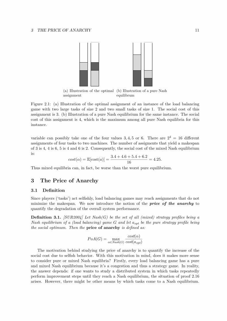
Suppose that there are two identical machines that have both speed 1 and four tasks, twosmall tasks of weight 1 and two large tasks of weight 2. An optimal assignment would map asmall and a large task to each of the machines so that the load on both machines is 3. Thisassignment is illustrated in figure 2.1a.
Now consider a pure strategy profile a that maps the two large tasks to the first machinesand the two small tasks to the second machine as illustrated in figure 2.1b. This way, thefirst machine has a load of 4 and the second machine has a load of 2. Obviously, a small taskcannot improve its cost by moving from the second to the first machine. A large task cannotimprove its cost by moving from the first tot the second machine either as its cost wouldremain 4 if it does. Thus this pure strategy profile a constitutes a pure Nash equilibrium withcost(a) = 4. This is a beautiful example to show the already stated statement that Nashequilibra aren’t mostly the optimal situations. Observe that all assigments that yield a largermakespan than 4 cannot be a Nash equilibrium as, in this case, one of the machines has aload of at least 5 and the other has a load of at most 1 so that moving any task from theformer to the latter would decrease the cost of this task. Thus, for this instance of the loadbalancing game, the social cost of the worst pure Nash Equilibrium is 4.
Clearly, the worst mixed equilibrium cannot be better than the worst pure equilibriumas the set of mixed equilibria is a superset of the set of pure equilibria, but can it really beworse? Suppose that each task is assigned to each of the machines with probability 1
2 . Thiscorresponds to a mixed strategy profile α with the αi’s being constant functions,
α =( 1
2︸︷︷︸α1
,12︸︷︷︸α2
,12︸︷︷︸α3
,12︸︷︷︸α4
)
. The expected load on machine j is thus:
`j(α) =∑
1≤i≤4wiαi(j) = 1
2 + 12 + 1 + 1 = 3
It’s important to notice that te expected cost of a task on a machine is larger than theexpected load of the machine, unless the task is assigned with probability 1 to this machine.For example, if we assume that task 1 is a small task, then:
U j1 = `j(α) + (1− α1(j))w1= 3 + 1
2 = 3.5
and, if task 3 is a large task, then:
U j3 = `j(α) + (1− α3(j))w3= 3 + 1
2 .2 = 4
For symmetry reasons, the expected cost of each task under the considered mixed strategyprofile α is the same on both machines so that α is a mixed Nash equilibrium. The social costof this equilibrium, cost(α), is defined to be the expected makespan, E[cost(a)], of the randompure assignment A induced by α. The makespan, cost(a), is in fact a random variable. This
3 THE PRICE OF ANARCHY 11
(a) Illustration of the optimalassignment
(b) Illustration of a pure Nashequilibrum
Figure 2.1: (a) Illustration of the optimal assignment of an instance of the load balancinggame with two large tasks of size 2 and two small tasks of size 1. The social cost of thisassignment is 3. (b) Illustration of a pure Nash equilibrium for the same instance. The socialcost of this assignment is 4, which is the maximum among all pure Nash equilibria for thisinstance.
variable can possibly take one of the four values 3, 4, 5 or 6. There are 24 = 16 differentassignments of four tasks to two machines. The number of assigments that yield a makespanof 3 is 4, 4 is 6, 5 is 4 and 6 is 2. Consequently, the social cost of the mixed Nash equilibriumis:
cost(α) = E[cost(a)] = 3.4 + 4.6 + 5.4 + 6.216 = 4.25.
Thus mixed equilibria can, in fact, be worse than the worst pure equilibrium.
3 The Price of Anarchy
3.1 Definition
Since players (‘tasks’) act selfishly, load balancing games may reach assignments that do notminimize the makespan. We now introduce the notion of the price of the anarchy toquantify the degradation of the overall system performance.
Definition 3.1. [SUR2004] Let Nash(G) be the set of all (mixed) strategy profiles being aNash equilibrium of a (load balancing) game G and let aopt be the pure strategy profile beingthe social optimum. Then the price of anarchy is defined as:
PoA(G) = maxα∈Nash(G)
cost(α)cost(aopt)
The motivation behind studying the price of anarchy is to quantify the increase of thesocial cost due to selfish behavior. With this motivation in mind, does it makes more senseto consider pure or mixed Nash equilibria? Firstly, every load balancing game has a pureand mixed Nash equilibrium because it’s a congestion and thus a strategy game. In reality,the answer depends: if one wants to study a distributed system in which tasks repeatedlyperform improvement steps until they reach a Nash equilibrium, the situation of proof 2.16arises. However, there might be other means by which tasks come to a Nash equilibrium.
3 THE PRICE OF ANARCHY 12
Moreover, the upper bounds about the price of anarchy for mixed equilibria are more robustthan upper bounds for pure equilibira as mixed equilibria are more general. We’ll study bothequilibria in two situations: the case in which all machines have an equal speed and the casethey don’t. It will be clear that if the server speeds are relatively bounded an the number oftask is large compared to the number of machines, then every Nash assignment approachesthe social optimum!
3.2 Bachmann-Landau notations
For understanding the four cases for which we’ll study the price of the anarchy, it’s importantto know the Bachmann-Landau notations. These notation are used to describe the limitingbehavior of a function in terms of simpler functions. These notations are used a lot incomputer science to classify algorithms by how they respond to change in input size.
3.2.1 Bigh Oh, Big Omega & Big Theta
Definition 3.2. (Big Oh)[MEU2011]Big Oh is the set of all functions f that are bounded above by g asymptotically (up to constantfactor).
O(g(n)) = f |∃c, n0 ≥ 0 : ∀n ≥ n0 : 0 ≤ f(n) ≤ cg(n)
We now proof a very simple lemma to show that indeed constant factors doesn’t matterfor Big Oh:
Lemma 3.3. ∀k > 0 : O(k.g(n)) = O(g(n))
Proof.
O(k.g(n)) = f |∃c, n0 ≥ 0 : ∀n ≥ n0 : 0 ≤ f(n) ≤ k.c.g(n)= f |∃c, n0 ≥ 0 : ∀n ≥ n0 : 0 ≤ f(n) ≤ (k.c).g(n)
let c’ = k.c= f |∃c′, n0 ≥ 0 : ∀n ≥ n0 : 0 ≤ f(n) ≤ c′.g(n)= O(g(n))
Definition 3.4. (Big Omega)[MEU2011]Big Omega is the set of all functions f that are bounded below by g asymptotically (up toconstant factor).
Ω(g(n)) = f |∃c, n0 ≥ 0 : ∀n ≥ n0 : 0 ≤ cg(n) ≤ f(n)
Definition 3.5. (Big Theta)[MEU2011]Big Theta is the set of all functions f that are bounded above and below by g asymptotically(up to constant factors).
Θ(g(n)) = f |∃c1, c2 > 0, n0 ≥ 0 : ∀n ≥ n0 : 0 ≤ c1.g(n) ≤ f(n) ≤ c2.g(n)
3 THE PRICE OF ANARCHY 13
3.2.2 Small Oh, Small Omega & Small Theta
Definition 3.6. (Small Oh)[BIN1977]Small Oh is the set of all functions f that are dominated by g asymptotically.
o(g(n)) = f |∀ε > 0, ∃n0∀n ≥ n0 : f(n) ≤ ε.g(n)
Equivalent definitions for small omega & small theta can easily be found. Note that thesmall oh-notation is a much stronger statement than the corresponding big oh-notation: everyfunction that is in the small oh of g is also in big oh, but the inverse isn’t necessarily true.Intuitively, f(x) ∈ o(g(x)) means that g(x) grows much faster than f(x).
3.2.3 Asymptotical Equality
Definition 3.7. (Asymptotically Equal)[BIN1977]
Let f and g real functions, then f is asymptotically equal to g ⇔ limx→+∞
f(x)g(x) = 1. Notation:
f ∼ g.In fact asymptotical equality, can also be defined as an equivalency relation: f ∼ g ⇔
(f − g) ∈ o(g). It’s trivially clear that as f ∼ g ⇒ f ∈ O(g).
3.3 PoA in Pure Nash Equilibria
3.3.1 Identical Machines
Theorem 3.8. Let G be a load balancing game with n tasks of weight w1, ..., wn and midentical machines. Under a pure Nash equilibrium a ∈ A it holds:
cost(a)cost(aopt)
≤ 2− 2m+ 1
Proof. Let j∗ be a machine with the highest load under profile a, and let i∗ be a task ofsmallest weight assigned to this machine. WLOG, there are at least two tasks assigned tomachine j∗ as, otherwise, cost(a) = cost(aopt) so that the upper bound given in the theoremfollows trivially. Thus wi∗ ≤ 1
2cost(a).
Suppose there is a machine j ∈ [m]\j∗ with load less than lj∗ − wi∗ . Then moving thetask i∗ from j∗ to j would decrease the cost for this task. Hence, as a is a Nash equilibriumit holds:
`j ≥ `j∗ − wi∗ ≥ cost(a)− 12cost(a) = 1
2cost(a).
Now observe that the cost of an optimal assignment cannot be smaller than the averageload over all machines, so:
cost(aopt) ≥∑i∈[n]wi
m
=∑j∈[m] `j
m
≥cost(a) + 1
2cost(a)(m− 1)m
= (m+ 1)cost(a)2m
3 THE PRICE OF ANARCHY 14
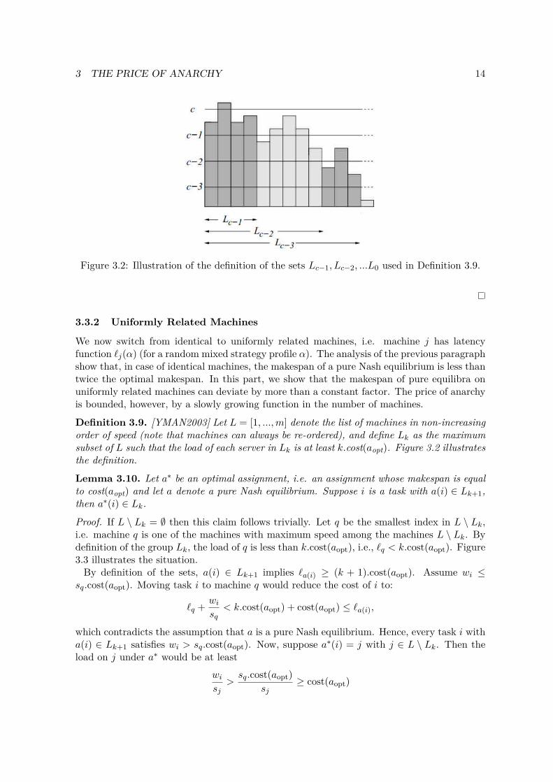
Figure 3.2: Illustration of the definition of the sets Lc−1, Lc−2, ...L0 used in Definition 3.9.
3.3.2 Uniformly Related Machines
We now switch from identical to uniformly related machines, i.e. machine j has latencyfunction `j(α) (for a random mixed strategy profile α). The analysis of the previous paragraphshow that, in case of identical machines, the makespan of a pure Nash equilibrium is less thantwice the optimal makespan. In this part, we show that the makespan of pure equilibra onuniformly related machines can deviate by more than a constant factor. The price of anarchyis bounded, however, by a slowly growing function in the number of machines.
Definition 3.9. [YMAN2003] Let L = [1, ...,m] denote the list of machines in non-increasingorder of speed (note that machines can always be re-ordered), and define Lk as the maximumsubset of L such that the load of each server in Lk is at least k.cost(aopt). Figure 3.2 illustratesthe definition.
Lemma 3.10. Let a∗ be an optimal assignment, i.e. an assignment whose makespan is equalto cost(aopt) and let a denote a pure Nash equilibrium. Suppose i is a task with a(i) ∈ Lk+1,then a∗(i) ∈ Lk.
Proof. If L \ Lk = ∅ then this claim follows trivially. Let q be the smallest index in L \ Lk,i.e. machine q is one of the machines with maximum speed among the machines L \ Lk. Bydefinition of the group Lk, the load of q is less than k.cost(aopt), i.e., `q < k.cost(aopt). Figure3.3 illustrates the situation.
By definition of the sets, a(i) ∈ Lk+1 implies `a(i) ≥ (k + 1).cost(aopt). Assume wi ≤sq.cost(aopt). Moving task i to machine q would reduce the cost of i to:
`q + wisq
< k.cost(aopt) + cost(aopt) ≤ `a(i),
which contradicts the assumption that a is a pure Nash equilibrium. Hence, every task i witha(i) ∈ Lk+1 satisfies wi > sq.cost(aopt). Now, suppose a∗(i) = j with j ∈ L \ Lk. Then theload on j under a∗ would be at least
wisj
>sq.cost(aopt)
sj≥ cost(aopt)

3 THE PRICE OF ANARCHY 15
Figure 3.3: Illustration of the sets Lk and Lk+1 and the machine q used in the proof of Lemma3.10.
because sj ≤ sq. However, this contradicts that a∗ is an optimal assignment. Consequently,a∗(i) ∈ Lk.
Γ−1 denotes the inverse of the gamma function, an extension of the factorial function withthe property that Γ(k) = (k − 1)!, for every positive integer k. In the rest of this paper, thefollowing property of Γ−1 will be used several times:
Lemma 3.11. ∀m ∈ R : Γ−1(m) ∈ O(
logmlog logm
).
Proof. Let Γ−1(m) = k, then k! is the greatest factorial smaller or equal to m, by definitionof the (general) gamma function (Γ(z) =
∫∞0 tz−1e−t dt). Because m ∼ k! and k! ∼ kk we get:
⇒ m ∼ kk
⇒ logm ∼ k log(k)
⇒ k ∼ logmlog(k)
⇒ k ∼ logmlog( logm
log(k))
⇒ k ∼ logmlog logm− log log(k)
Remember that, when using O(...), constant factors don’t matter by Definition 3.3, and anyterm that grows more slowly than another term can be abandoned by definition, becausem > k:
⇒ k ∼ logmlog logm
So thatΓ−1(m) ∈ O
( logmlog logm
)
3 THE PRICE OF ANARCHY 16
Theorem 3.12. Let G be a load balancing game with n tasks of weight w1, ..., wn and mmachines of speed s1, ..., sm. Let a denote a pure Nash equilibrium. Then, it holds that:
cost(a)cost(aopt)
∈ O( logm
log logm
)Proof. Let
c =⌊cost(α)
cost(aopt)
⌋.
We show c ≤ Γ−1(m). This yields the theorem as in Lemma 3.11:
Γ−1(m) ∈ Θ( logm
log logm
).
WLOG, let us assume s1 ≥ s2 ≥ ... ≥ sm and let L = [1, 2, ...,m] denote the list of machines innon-increasing order of speed. With definition 3.9 in mind, we will show the follow recurrenceon the lengths of the sets Lk:
|Lk| ≥ (k + 1)|Lk+1| (0 ≤ k ≤ c− 2)|Lc−1| ≥ 1
Solving the recurrence yields |L0| ≥ (c − 1)! = Γ(c). Now observe that Lo = L, and, hence,|Lo| = m. Consequently, m ≥ Γ(c) so that c ≤ Γ−1(m), which proves the statement.
It remains to prove the recurrence. We first prove |Lc−1| ≥ 1. Assume Lc−1 = ∅, then theload of machine 1 is less than (c− 1).cost(aopt). Moving i to machine 1 reduces the cost of ito strictly less than
(c− 1).cost(aopt) + wis1≤ (c− 1).cost(aopt) + cost(aopt) ≤ c.cost(aopt)
where the inequality wis1≤ cost(aopt) follows from the fact that s1 is the speed of the fastest
machine. Consequently, player i is able to unilaterally decrease its cost by moving its taskfrom machine j to machine 1, which contradicts the assumption that α is a mixed Nash equi-librium. Thus, we have shown that |Lc−1| ≥ 1.
Next, we show |Lk| ≥ (k + 1)|Lk+1|, for 0 ≤ k ≤ c− 2. Let a∗ be an optimal assignment,i.e., an assignment whose makespan is equal to cost(aopt). By definition of Lk+1, the sum ofthe weights that a assigns to a machine j ∈ Lk+1 is at least (k + 1).cost(aopt).sj . Hence, thetotal weight assigned to the machines in Lk+1 is at least
∑j∈Lk+1
(k + 1).cost(aopt).sj . Bylemma 3.10 an optimal assignment has to assign all this weight to the machines in Lk suchthat the load on each of these machines is at most cost(aopt). As a consequence,∑
j∈Lk+1
(k + 1).cost(aopt).sj ≤∑j∈Lk
cost(aopt).sj
Dividing by cost(aopt) and substracting∑j∈Lk+1
sj from both sides yields∑j∈Lk+1
k.sj ≤∑
j∈Lk\Lk+1
sj
3 THE PRICE OF ANARCHY 17
Now let s∗ denote the speed of the slowest machine in Lk+1, i.e., s∗ = s|Lk+1|. For allj ∈ Lk+1, sj ≥ s∗, and, for all j ∈ Lk \ Lk+1, sj ≤ s∗. Hence, we obtain∑
j∈Lk+1
k.s∗ ≤∑
j∈Lk\Lk+1
s∗,
which implies |Lk+1|.k ≤ |Lk \ Lk+1| = |Lk| − |Lk+1|. Thus, |Lk| ≥ (k + 1).|Lk+1|.
We now prove a lower bound for the price of anarchy for pure Nash equilibria for uniformlyrelated machines. This lower bound is important, because it shows us that the upper boundon the price of anarchy given in Theorem 3.12 is essentially tight.
Theorem 3.13. For every m ∈ N, there exists an instance of G of the load balancing gamewith m machines and n ≤ m tasks that has a pure Nash equilibrium a with:
cost(a)cost(aopt)
∈ Ω( logm
log logm
)Proof. We will describe in this proof a game instance G together with an equilibrium assign-ment a satisfying
cost(a)cost(aopt)
≥ 12(Γ−1(m)− 2− o(1)
)which yields the theorem. Our construction uses q + 1 disjoint sets of machines denotedG0, ..., Gq with q ≈ Γ−1(m). More, precisely, we set
q =⌊Γ−1(m3 )− 1
⌋≥ Γ−1(m)− 2− o(1).
For 0 ≤ k ≤ q, group Gk consists of q!/k! machines of speed 2k each of which is assigned ktasks of weight 2k. The total number of machines in these groups is thus:
q∑k=0|Gk| = q!
q∑k=0
1k! ≤ 3Γ(q + 1) ≤ m
because∑qk=0
1k! ≤ 3 and 3Γ(q+1) ≤ m, which follows directly from the definition of q. As m
might be larger than the number of the machines in the sets, there might be some machinesthat do not belong to any of the groups. We assume that these machines have the sameparameters as the machines in group G0: i.e., they have speed 20 = 1 and a does not assigntasks to them.We need to show that the described assignment is a pure Nash equilibrium. A task on amachine from set Gk has cost k. It can neither reduce its cost by moving its task to amachine in Gj with j ≥ k as these machines have at least a load of k, nor can it reduce itscost by moving its task to a machine in group Gj with j < k as the load on such a machine,after the task moved to this machine, would be:
j + 2k
2j = j + 2k−j ≥ j + (k − j + 1) = k + 1
since 2t ≥ t + 1, for every t ≥ 1. Hence, none of the tasks can unilaterally decrease its cost.In other words, a is a pure Nash equilibrium. The social cost or makespan of the equilibrium
3 THE PRICE OF ANARCHY 18
a is q. Next, we show that cost(aopt) ≤ 2 so that the theorem follows. We construct anassignment or strategy profile with load at moast 2 on every machine. For each k ∈ 1, ..., q,the task mapped by A to the machines in Gk are now assigned tot the machines in Gk−1.Observe that the total number of tasks that a maps to the machines in Gk is
k|Gk| = kq!k! = q!
(k − 1)! = |Gk−1|.
Hence, we can assign the tasks in such a way that each machine in group Gk−1 receives exactlyone of the tasks that A mapped to a machine in group Gk. This task has a weight of 2k andthe speed of the machine is 2k−1. Hence, the load of each machine in this assignment is atmost 2, which completes the proof.
Theorem 3.12 gives an upper bound and Theorem 3.13 gives a lower bound for the priceof anarchy for pure equilibria on uniformly related machines, so we conclude ∀G with a pureequilibrium:
PoA(G) ∈ Θ( logm
log logm
)
3.4 PoA in Mixed Nash Equilibria
3.4.1 Identical Machines
In the following paragraph, we will prove a bound for the PoA(G) for a mixed Nash Equi-librium. The proof uses the weighted Chernoff Bound theorem and Boole’s inequality fromprobability theory. The weighted Chernoff Bound will not be proved in this paper.
Theorem 3.14. weighted Chernoff Bound Let X1, ....Xn be independent random variableswith values in the interval [0, z] for some z > 0, and let X =
∑ni=1Xi, then for any t it holds
that P[∑ni=1Xi ≥ t] ≤ (e.E[X]/t)t/z.
Theorem 3.15. Boole’s inequality[GAL1996] For a countable set of events A1, ..., An wehave:
P(⋃
i
Ai
)≤∑i
P(Ai).
Proof. Boole’s inequality may be proved using the method of induction.For the n = 1 case, it follows that P(A1) ≤ P(A1).For the case n+ 1, we have
P(n+1⋃i=1
Ai
)≤
n+1∑i=1
P(Ai).
Since P(A ∪ B) = P(A) + P(B) − P(A ∩ B), and because the union operation is associative,we have
P(n+1⋃i=1
Ai
)= P
( n⋃i=1
Ai
)+ P(An+1)− P
( n⋃i=1
Ai ∩An+1
).
Since P(⋃n
i=1 Ai ∩An+1
)≥ 0, as is the case for any probability measure, we have
P(n+1⋃i=1
Ai
)≤ P
( n⋃i=1
Ai
)+ P(An+1)
3 THE PRICE OF ANARCHY 19
, and therefore
P(n+1⋃i=1
Ai
)≤
n∑i=1
P(Ai) + P(An+1) =n+1∑i=1
P(Ai)
.
Theorem 3.16. Let G be a load balancing game with n tasks of weight w1, ..., wn and mmachines of equal speed. Let α denote a mixed Nash equilibrium. Then, it holds that:
cost(α)cost(aopt)
∈ O( logm
log logm
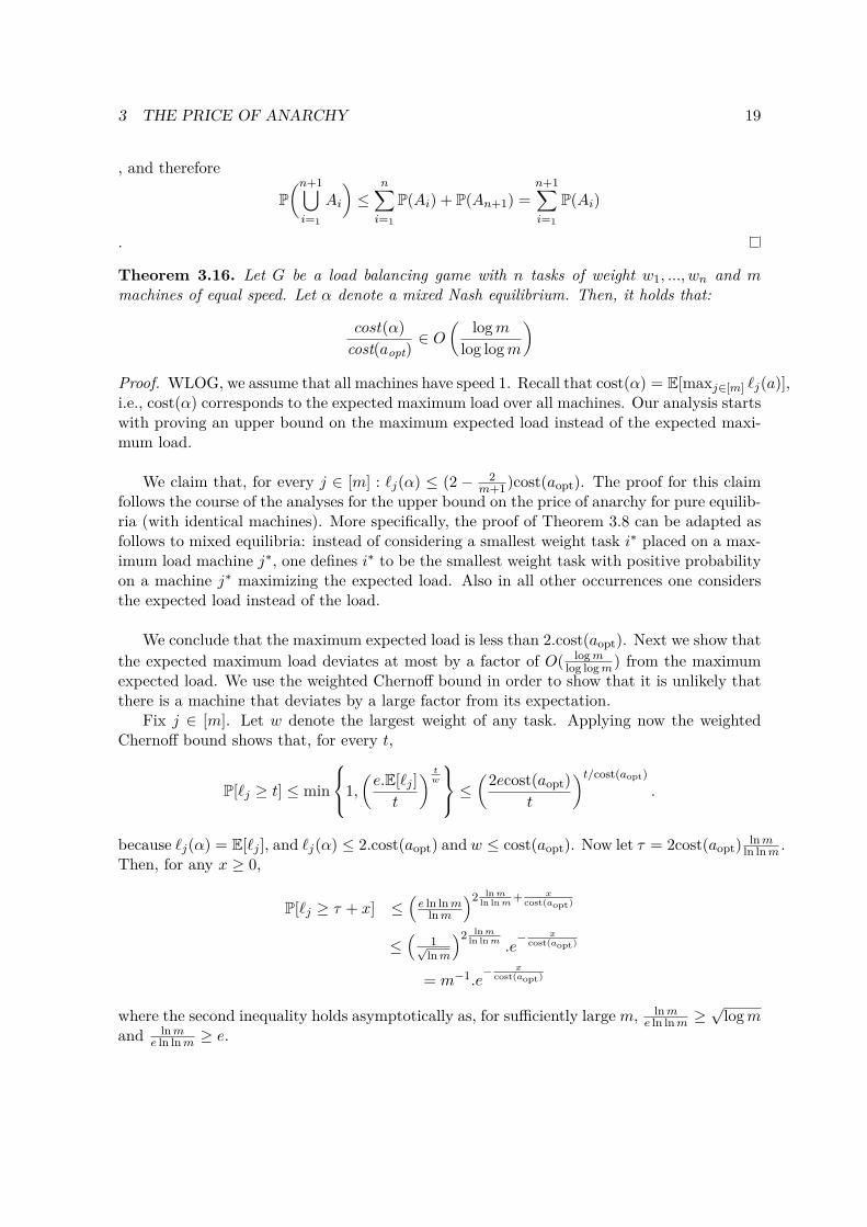
)Proof. WLOG, we assume that all machines have speed 1. Recall that cost(α) = E[maxj∈[m] `j(a)],i.e., cost(α) corresponds to the expected maximum load over all machines. Our analysis startswith proving an upper bound on the maximum expected load instead of the expected maxi-mum load.
We claim that, for every j ∈ [m] : `j(α) ≤ (2 − 2m+1)cost(aopt). The proof for this claim
follows the course of the analyses for the upper bound on the price of anarchy for pure equilib-ria (with identical machines). More specifically, the proof of Theorem 3.8 can be adapted asfollows to mixed equilibria: instead of considering a smallest weight task i∗ placed on a max-imum load machine j∗, one defines i∗ to be the smallest weight task with positive probabilityon a machine j∗ maximizing the expected load. Also in all other occurrences one considersthe expected load instead of the load.
We conclude that the maximum expected load is less than 2.cost(aopt). Next we show thatthe expected maximum load deviates at most by a factor of O( logm
log logm) from the maximumexpected load. We use the weighted Chernoff bound in order to show that it is unlikely thatthere is a machine that deviates by a large factor from its expectation.
Fix j ∈ [m]. Let w denote the largest weight of any task. Applying now the weightedChernoff bound shows that, for every t,
P[`j ≥ t] ≤ min
1,(e.E[`j ]t
) tw
≤(2ecost(aopt)
t
)t/cost(aopt).
because `j(α) = E[`j ], and `j(α) ≤ 2.cost(aopt) and w ≤ cost(aopt). Now let τ = 2cost(aopt) lnmln lnm .
Then, for any x ≥ 0,
P[`j ≥ τ + x] ≤(e ln lnm
lnm
)2 ln mln ln m
+ xcost(aopt)
≤(
1√lnm
)2 ln mln ln m .e
− xcost(aopt)
= m−1.e− x
cost(aopt)
where the second inequality holds asymptotically as, for sufficiently large m, lnme ln lnm ≥
√logm
and lnme ln lnm ≥ e.
3 THE PRICE OF ANARCHY 20
Now we can upper-bound cost(α) as follows. For every nonnegative random variable X,E[X] =
∫∞0 P[X ≥ t]dt. Consequently,
cost(α) = E[
maxj∈[m]
`j(a)]
=∫ ∞
0P[maxj∈[m]
`j(a) ≥ t]dt.
Substituting t by τ + x and then applying the union bound yields:
cost(α) ≤ τ +∫ ∞
0P[maxj∈[m]
`j(a) ≥ τ + x]dx ≤∫ ∞
0P[`j(a) ≥ τ + x]dx
, Finally, we apply the tail bound derived above and obtain
cost(P ) ≤ τ +∫ ∞
0e
−xcost(aopt)dx = τ + cost(aopt),
which yields the theorem as τ = 2cost(aopt) lnmln lnm .
From a purely mathematical point of view, it’s necessary to proof also the lower boundin mixed Nash equilibria to conclude that Pa(α) ∈ Θ( logm
log logm) for identical machines, butpure intuitively we can also use the fact that pure Nash equilibria reduce the level of anarchy,unlike mixed equilibria who increase the price. So, with Theorem 3.13, we conclude for mixedstrategies on identical machines:
PoA(G) ∈ Θ( logm
log logm
)
3.4.2 Uniformly Related Machines
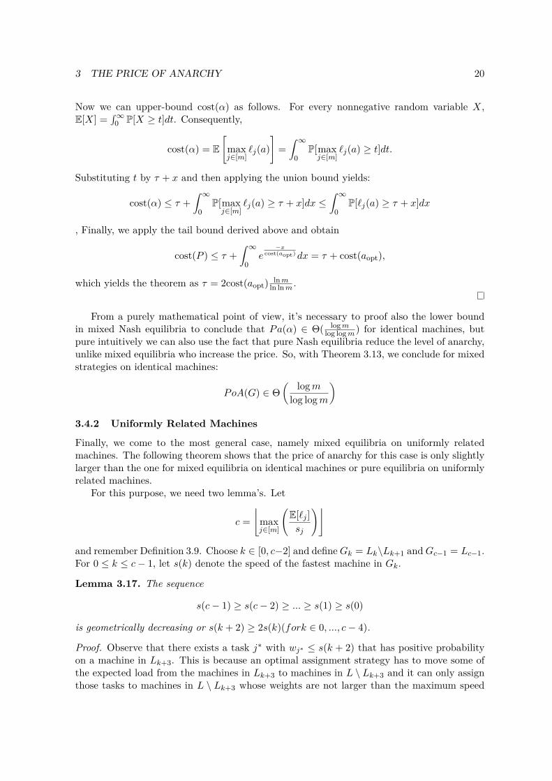
Finally, we come to the most general case, namely mixed equilibria on uniformly relatedmachines. The following theorem shows that the price of anarchy for this case is only slightlylarger than the one for mixed equilibria on identical machines or pure equilibria on uniformlyrelated machines.
For this purpose, we need two lemma’s. Let
c =⌊
maxj∈[m]
(E[`j ]sj
)⌋
and remember Definition 3.9. Choose k ∈ [0, c−2] and defineGk = Lk\Lk+1 andGc−1 = Lc−1.For 0 ≤ k ≤ c− 1, let s(k) denote the speed of the fastest machine in Gk.
Lemma 3.17. The sequence
s(c− 1) ≥ s(c− 2) ≥ ... ≥ s(1) ≥ s(0)
is geometrically decreasing or s(k + 2) ≥ 2s(k)(fork ∈ 0, ..., c− 4).
Proof. Observe that there exists a task j∗ with wj∗ ≤ s(k + 2) that has positive probabilityon a machine in Lk+3. This is because an optimal assignment strategy has to move some ofthe expected load from the machines in Lk+3 to machines in L \ Lk+3 and it can only assignthose tasks to machines in L \ Lk+3 whose weights are not larger than the maximum speed
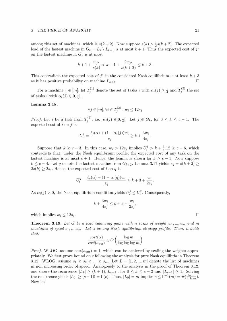
3 THE PRICE OF ANARCHY 21
among this set of machines, which is s(k + 2). Now suppose s(k) > 12s(k + 2). The expected
load of the fastest machine in Gk = Lk \ Lk+1 is at most k + 1. Thus the expected cost of j∗on the fastest machine in Gk is at most
k + 1 + wj∗
s(k) < k + 1 + 2wj∗s(k + 2) ≤ k + 3.
This contradicts the expected cost of j∗ in the considered Nash equilibrium is at least k + 3as it has positive probability on machine Lk+3.
For a machine j ∈ [m], let T (1)j denote the set of tasks i with αi(j) ≥ 1
4 and T(2)j the set
of tasks i with αi(j) ∈]0, 14 [.
Lemma 3.18.∀j ∈ [m], ∀i ∈ T (2)
j : wi ≤ 12sj
Proof. Let i be a task from T(2)j , i.e. αi(j) ∈]0, 1
4 [. Let j ∈ Gk, for 0 ≤ k ≤ c − 1. Theexpected cost of i on j is:
U ji = `j(α) + (1− αi(j))wisj
≥ k + 3wi4sj
.
Suppose that k ≥ c − 3. In this case, wi > 12sj implies U ji > k + 34 .12 ≥ c + 6, which
contradicts that, under the Nash equilibrium profile, the expected cost of any task on thefastest machine is at most c + 1. Hence, the lemma is shown for k ≥ c − 3. Now supposek ≤ c− 4. Let q denote the fastest machine from Gk+2. Lemma 3.17 yields sq = s(k + 2) ≥2s(k) ≥ 2sj . Hence, the expected cost of i on q is
U qi = `q(α) + (1− αi(q))wisq
≤ k + 3 + wi2sj
.
As αi(j) > 0, the Nash equilibrium condition yields U ji ≤ Uqi . Consequently,
k + 3wi4sj≤ k + 3 + wi
2sj,
which implies wi ≤ 12sj .
Theorem 3.19. Let G be a load balancing game with n tasks of weight w1, ..., wn and mmachines of speed s1, ..., sm. Let α be any Nash equilibrium strategy profile. Then, it holdsthat:
cost(α)cost(aopt)
∈ O( logm
log log logm
)Proof. WLOG, assume cost(aopt) = 1, which can be achieved by scaling the weights appro-priately. We first prove bound on c following the analysis for pure Nash equilibria in Theorem3.12. WLOG, assume s1 ≥ s2 ≥ ... ≥ sm. Let L = [1, 2, ...,m] denote the list of machinesin non increasing order of speed. Analogously to the analysis in the proof of Theorem 3.12,one shows the recurrence |Lk| ≥ (k + 1).|Lk+1|, for 0 ≤ k ≤ c − 2 and |Lc−1| ≥ 1. Solvingthe recurrence yields |L0| ≥ (c− 1)! = Γ(c). Thus, |L0| = m implies c ≤ Γ−1(m) = Θ( lnm
ln lnm).Now let

3 THE PRICE OF ANARCHY 22
C = maxc+ 1, lnm
ln lnm
= Θ
( lnmln lnm
)In the rest of the proof, we show that the expected makespan of the equilibrium assignment
can exceed C at most by a factor of order ln lnm/ ln ln lnm so that the expected makespanis O(lnm/ ln ln lnm), which proves the theorem as we assume cost(aopt) = 1.
As the next step, we prove a tail bound on `j(α)sj
, for any fixed j ∈ [m] and, afterward, weuse this tail bound to derive an upper bound on the expected makespan.
Let `(1)j and `
(2)j
sjdenote random variables that the describe the load on link j only taking
into account the tasks T (1)j and T
(2)j , respectively. Observe that `j(α)
sj= `
(1)j (α)sj
+ `(2)j (α)sj
. For
the tasks in T(1)j , we immediately obtain
`(1)j
sj≤
∑i∈T (1)
j
wisj≤ 4
∑i∈T (1)
j
wipji
sj= 4E[`
(1)jsj
] ≤ 4C. (1)
To prove an upper bound on `(2)j
sj, we use the weighted Chernoff bound from Lemma 3.14.
This bound requires an upper bound on the maximum weight. As a first step to bound theweights, we prove a result about the relationship between the speeds of the machines in thedifferent groups that are defined by the prefixes. For 0 ≤ k ≤ c−2, let Gk = Lk\Lk+1, and letGc−1 = Lc−1. For 0 ≤ k ≤ c− 1, let s(k) denote the speed of the fastest machine in Gk. By,Lemma 3.17, we know that this sequence is geometrically decreasing. Let z = max
i∈T (2)j
(wisj
.Lemma 3.18 implies z ≤ 12. Now applying the weighted Chernoff bound from Lemma 3.14yields that, for every ϕ > 0
P[`
(2)j /sj ≥ ϕC
]≤
eE[`(2)j /sj ]ϕC
ϕC/z ≤ ( eϕ
)ϕC/12
since E[ `(2)j
sj] ≤ C. We define τ = 24C ln lnm/ ln ln lnm. As C is of order lnm/ ln lnm, it
follows that τ is of order lnm/ ln ln lnm. Let x ≥ 0. We substitute τ + x for ϕC and obtain:
P[`
(2)j /sj ≥ τ + x
]≤
(eC
τ + x
)
≤(e ln ln lnm24 ln lnm
)2C ln ln mln ln ln m
+ x12
Observe that 24 ln lnm/(e ln ln lnm) is lower bounded by√
ln lnm and also lower boundedby e2. Furthermore, C ≥ lnm/ ln lnm. Applying these bounds yields
P[`
(2)j /sj ≥ τ + x
]≤( 1√
ln lnm
)2 ln mln ln ln m
.e−x/6 = m−1.e−x/6
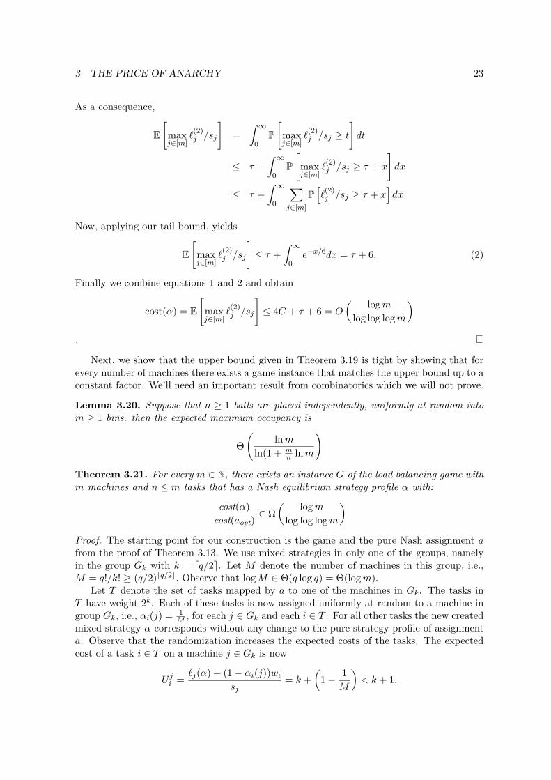
3 THE PRICE OF ANARCHY 23
As a consequence,
E[
maxj∈[m]
`(2)j /sj
]=
∫ ∞0
P[
maxj∈[m]
`(2)j /sj ≥ t
]dt
≤ τ +∫ ∞
0P[
maxj∈[m]
`(2)j /sj ≥ τ + x
]dx
≤ τ +∫ ∞
0
∑j∈[m]
P[`
(2)j /sj ≥ τ + x
]dx
Now, applying our tail bound, yields
E[
maxj∈[m]
`(2)j /sj
]≤ τ +
∫ ∞0
e−x/6dx = τ + 6. (2)
Finally we combine equations 1 and 2 and obtain
cost(α) = E[
maxj∈[m]
`(2)j /sj
]≤ 4C + τ + 6 = O
( logmlog log logm
).
Next, we show that the upper bound given in Theorem 3.19 is tight by showing that forevery number of machines there exists a game instance that matches the upper bound up to aconstant factor. We’ll need an important result from combinatorics which we will not prove.
Lemma 3.20. Suppose that n ≥ 1 balls are placed independently, uniformly at random intom ≥ 1 bins. then the expected maximum occupancy is
Θ(
lnmln(1 + m
n lnm
)
Theorem 3.21. For every m ∈ N, there exists an instance G of the load balancing game withm machines and n ≤ m tasks that has a Nash equilibrium strategy profile α with:
cost(α)cost(aopt)
∈ Ω( logm
log log logm
)Proof. The starting point for our construction is the game and the pure Nash assignment afrom the proof of Theorem 3.13. We use mixed strategies in only one of the groups, namelyin the group Gk with k = dq/2e. Let M denote the number of machines in this group, i.e.,M = q!/k! ≥ (q/2)bq/2c. Observe that logM ∈ Θ(q log q) = Θ(logm).
Let T denote the set of tasks mapped by a to one of the machines in Gk. The tasks inT have weight 2k. Each of these tasks is now assigned uniformly at random to a machine ingroup Gk, i.e., αi(j) = 1
M , for each j ∈ Gk and each i ∈ T . For all other tasks the new createdmixed strategy α corresponds without any change to the pure strategy profile of assignmenta. Observe that the randomization increases the expected costs of the tasks. The expectedcost of a task i ∈ T on a machine j ∈ Gk is now
U ji = `j(α) + (1− αi(j))wisj
= k +(
1− 1M
)< k + 1.
4 COORDINATIONS MECHANISMS 24
In the proof of Theorem 3.13, we have shown that the cost of a task i of weight 2k on amachine of group Gj with j 6= k is at least k + 1. Thus, the mixed strategy profile α is aNash equilibrium.
It remains to compare the social cost of the equilibrium profile α with the optimal cost.The structure of the optimal assignment is not affected by the modifications. It has socialscost cost(aopt) = 2. Now we give a lower bound for the social cost of α. This social cost is,obviously, bounded from below by the maximum number of tasks that are mapped to thesame machine in the group Gk. Applying Lemma ?? with M bins and N = kM balls showsthat the expected makespan is:
Ω(
lnMln(1 + 1
k lnM)
)= Ω
( logmlog log logm
),
where the last estimate holds as k ∈ Θ(logm/ log logm) and logM = Θ(logm). T
Theorem 3.19 gives an upper bound and Theorem 3.21 gives a lower bound for the priceof anarchy for mixed equilibria on uniformly related machines, so we conclude ∀G with anequilibrium:
PoA(G) ∈ Θ( logm
log log logm
)
3.5 Summary
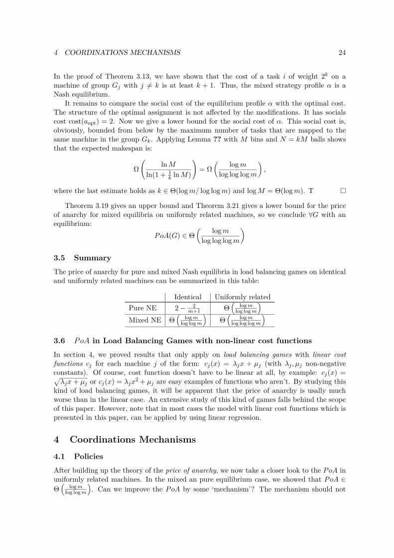
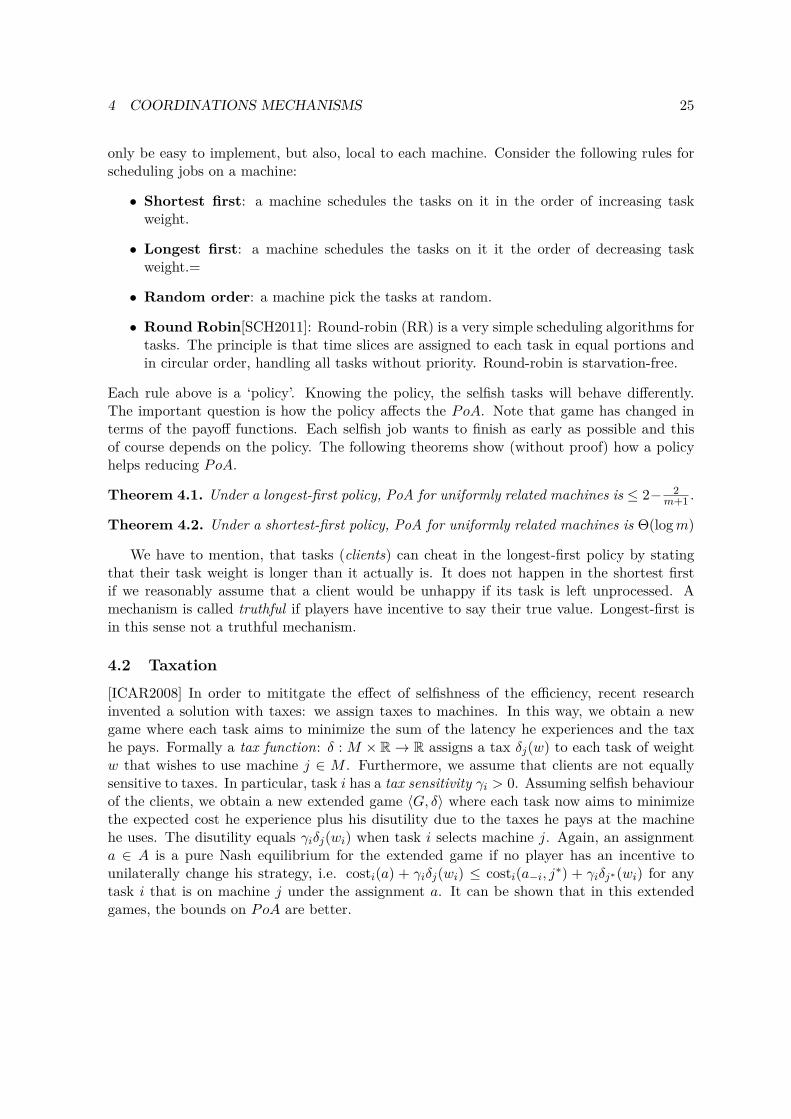
The price of anarchy for pure and mixed Nash equilibria in load balancing games on identicaland uniformly related machines can be summarized in this table:
Identical Uniformly relatedPure NE 2− 2
m+1 Θ(
logmlog logm
)Mixed NE Θ
(logm
log logm
)Θ(
logmlog log logm
)3.6 PoA in Load Balancing Games with non-linear cost functions
In section 4, we proved results that only apply on load balancing games with linear costfunctions cj for each machine j of the form: cj(x) = λjx + µj (with λj , µj non-negativeconstants). Of course, cost function doesn’t have to be linear at all, by example: cj(x) =√λjx+ µj or cj(x) = λjx
2 + µj are easy examples of functions who aren’t. By studying thiskind of load balancing games, it will be apparent that the price of anarchy is usally muchworse than in the linear case. An extensive study of this kind of games falls behind the scopeof this paper. However, note that in most cases the model with linear cost functions which ispresented in this paper, can be applied by using linear regression.
4 Coordinations Mechanisms
4.1 Policies
After building up the theory of the price of anarchy, we now take a closer look to the PoA inuniformly related machines. In the mixed an pure equilibrium case, we showed that PoA ∈Θ(
logmlog logm
). Can we improve the PoA by some ‘mechanism’? The mechanism should not
4 COORDINATIONS MECHANISMS 25
only be easy to implement, but also, local to each machine. Consider the following rules forscheduling jobs on a machine:
• Shortest first: a machine schedules the tasks on it in the order of increasing taskweight.
• Longest first: a machine schedules the tasks on it it the order of decreasing taskweight.=
• Random order: a machine pick the tasks at random.
• Round Robin[SCH2011]: Round-robin (RR) is a very simple scheduling algorithms fortasks. The principle is that time slices are assigned to each task in equal portions andin circular order, handling all tasks without priority. Round-robin is starvation-free.
Each rule above is a ‘policy’. Knowing the policy, the selfish tasks will behave differently.The important question is how the policy affects the PoA. Note that game has changed interms of the payoff functions. Each selfish job wants to finish as early as possible and thisof course depends on the policy. The following theorems show (without proof) how a policyhelps reducing PoA.
Theorem 4.1. Under a longest-first policy, PoA for uniformly related machines is ≤ 2− 2m+1 .
Theorem 4.2. Under a shortest-first policy, PoA for uniformly related machines is Θ(logm)
We have to mention, that tasks (clients) can cheat in the longest-first policy by statingthat their task weight is longer than it actually is. It does not happen in the shortest firstif we reasonably assume that a client would be unhappy if its task is left unprocessed. Amechanism is called truthful if players have incentive to say their true value. Longest-first isin this sense not a truthful mechanism.
4.2 Taxation
[ICAR2008] In order to mititgate the effect of selfishness of the efficiency, recent researchinvented a solution with taxes: we assign taxes to machines. In this way, we obtain a newgame where each task aims to minimize the sum of the latency he experiences and the taxhe pays. Formally a tax function: δ : M × R→ R assigns a tax δj(w) to each task of weightw that wishes to use machine j ∈ M . Furthermore, we assume that clients are not equallysensitive to taxes. In particular, task i has a tax sensitivity γi > 0. Assuming selfish behaviourof the clients, we obtain a new extended game 〈G, δ〉 where each task now aims to minimizethe expected cost he experience plus his disutility due to the taxes he pays at the machinehe uses. The disutility equals γiδj(wi) when task i selects machine j. Again, an assignmenta ∈ A is a pure Nash equilibrium for the extended game if no player has an incentive tounilaterally change his strategy, i.e. costi(a) + γiδj(wi) ≤ costi(a−i, j∗) + γiδj∗(wi) for anytask i that is on machine j under the assignment a. It can be shown that in this extendedgames, the bounds on PoA are better.
REFERENCES 26
References
[BVOCK2007] B. Vocking, Selfish Load Balancing, Chapter 20 in Algorithmic Game Theory,Cambridge University Press, December 2007.
[JOARU1994] d J. Osborne and A. Rubinstein, A course in Game Theory, The MIT Press,1994.
[MANN2008] S. Mannor, Advancded Topics in Systems, Learning and Control, Lecture 3:Lecture 3: Mixed Actions, Nash and Correlated Equilibria, Technicon, November 2008.
[COL2011] E. Colebunders, Analyse II, Vrije Universiteit Brussel, 2011.
[CW2007] C. Witteveen, Intreerede: De Prijs van de Onafhankelijkheid, TU Delft 2007.
[YMAN2003] Y. Mansour, Lecture 6: Congestion and potential games, Computational Learn-ing Theory, University of Tel Aviv, 2003.
[JMAR] Jason R. Marden, Lecture 12: Game Theory Course, University of Colorado.
[THAR2011] T. Harks, M. Klimm, R. H. Mohring, Characterizing the Existence of PotentialFunctions in Weighted Congestion Games, February 2011
[ROSENTHAL73] R. W. Rosenthal, A class of games possessing pure-strategy Nash equilib-ria. International Journal of Game Theory, 2:65âĂŞ67, 1973
[ETE2007] K. Etessami, Algorithmic Game Theory - Lecture 16 Best response dynamics andpure Nash Equilibria, University of Edingburgh, 2007.
[ICAR2008] I. Caragiannis, C. Kaklamanis, P. Kanellopoulos, Improving the Efficiency ofLoad Balancing Games through Taxes, University of Patras, 2008.
[SUR2004] S. Suri, C. D. Toth, Y. Zhou. Selfish Load Balancing and Atomic CongestionGames, University of California, 2004.
[MEU2011] W. De Meuter. Algoritmen en Datastructuren I, Vrije Universiteit Brussel, 2011.
[BIN1977] K.G. Binmore. Mathematical Analysis: A Straightforward Approach, CambridgeUniversitiy Press, 1977.
[GAL1996] Galambos, Janos, Simonelli. Bonferroni-Type Inequalities with Applications,Probability and Its Applications, Springer-Verlag, 1996.
[SHI2008] A. Shirazi, Algorithmic Game Theory: Coordination mechanisms, University ofIllinois, 2008.
[SCH2011] P. Schelkens, Syllabus: Computersystemen, Vrije Universiteit Brussel, 2011.