gamermann, d.; montagud aquino, a.; conejero casares, ja

Document downloaded from:

This paper must be cited as:

The final publication is available at

Copyright

http://dx.doi.org/10.1089/cmb.2013.0150

http://hdl.handle.net/10251/51205

Mary Ann Liebert

Gamermann, D.; Montagud Aquino, A.; Conejero Casares, JA.; Urchueguía Schölzel, JF.;Fernández De Córdoba Castellá, PJ. (2014). New approach for phylogenetic tree recoverybased on genome-scale metabolic networks. Journal of Computational Biology. 21(7):508-519. doi:10.1089/cmb.2013.0150.

Phylogenetic tree reconstruction from genome-scalemetabolic models

D. Gamermann∗1,2 , A. Montagud2 , J. A. Conejero2 , P. F. de Cordoba2 and J. F. Urchieguıa2

1Catedra Energesis de Tecnologıa Interdisciplinar, Universidad Catolica de Valencia San Vicente Martir,Guillem de Castro 94, E-46003, Valencia, Spain.2Instituto Universitario de Matematica Pura y Aplicada, Universidad Politecnica de Valencia,

Camino de Vera 14, 46022 Valencia, Spain.

Email: Daniel Gamermann∗- [email protected];

∗Corresponding author

Abstract

A wide range of applications and research has been done with genome-scale metabolic models. In this work

we describe a methodology for comparing metabolic networks constructed from genome-scale metabolic models

and how to apply this comparison in order to infer evolutionary distances between different organisms. Our

methodology allows a quantification of the metabolic differences between different species from a broad range of

families and even kingdoms. This quantification is then applied in order to reconstruct phylogenetic trees for sets

of various organisms.

1 Introduction

Metabolic models at the genome-scale are one of the pre-requisites for obtaining insight into the operation

and regulation of metabolism as a whole [1–4]. Uses of metabolic models embrace all aspects of biotechnology:

from food [5] to pharmaceutical [6] and biofuels [7–9]. Genome-scale metabolic network reconstruction is, in

essence, a systematic assembly and organization of all reactions which build up the metabolism of a given

organism. It usually starts with genome sequences in order to identify reactions and network topology. This

methodology also offers an opportunity to systematically analyse omics datasets in the context of cellular

metabolic phenotypes.

1

arX

iv:1

211.

7192

v1 [

q-bi

o.M

N]

30

Nov

201

2

Reconstructions have now been built for a wide variety of organisms, and have been used toward five

major ends [10]: contextualization of high-throughput data [4, 8, 9, 11], guidance of metabolic engineering

[12], directing hypothesis-driven discovery [17], interrogation of multi-species relationships [18], and network

property discovery [15].

Nowadays, phylogenies are becoming increasingly popular, being used in almost every branch of biol-

ogy [16]. Beyond representing the relationships among species in the tree of life, phylogenies are used to

describe relationships between paralogues in a gene family [17], histories of populations [18], the evolutionary

and epidemiological dynamics of pathogens [19,20], the genealogical relationship of somatic cells during dif-

ferentiation and cancer development [21] and even the evolution of language [22]. More recently, molecular

phylogenetics has become an indispensible tool for genome comparisons [23–25].

A phylogeny is a tree containing vertex that are connected by branches. Each branch represents the

persistence of a genetic lineage through time, and each vertex represents the birth of a new lineage. If

the tree represents the relationships among a group of species, then the vertex represent speciation events.

Phylogenetic trees are not directly observed and are instead inferred from sequence or other data. Phy-

logeny reconstruction methods are either distance-based or character-based. In distance matrix methods,

the distance between every pair of sequences is calculated, and the resulting distance matrix is used for tree

reconstruction. For a very instructive review, please refer to [16].

This work is organized as follows. In the next section we briefly explain the genome-scale models we

work with and how we define a parameter for comparing two models. Following that section, we explain how

we recover the phylogenetic tree from the comparison matrix obtained for many metabolic models. This

will be done taking into account the minimum spanning tree of a non-directed connected weighted network

associated to these metabolic models. In the section after that, we present the results and a brief study of the

sensibility of the comparison parameter, and in the last section we present a brief summary and overview.

2 Comparison between metabolic models

In a recent paper [26], it has been presented a method for automatically generate genome-scale metabolic

models from data contained in the KEGG [27] database. The method consists in searching the database for

genes and pathways present in an organism and download the corresponding set of chemical reactions. The

algorithm filters isosenzymes, or other repeated reactions, and may add missing reactions to a given pathway

using a probabilistic criterion based on the comparison of the organism’s pathway with the same pathway

in other organisms. In this work we are using data obtained from this platform, but the method described

2

can, in principle, be used with any set of metabolic models given that the compounds names in the models

follow the same standard (the same compound has the same name in all models).

The first step in our work is to construct for every metabolic model A a non-directed connected network

NA = (VA, EA) from the information contained in it. Here, VA stands for the set of vertex (nodes) of

A and EA for its set of edges. A metabolic model comprises a set of chemical reactions. Each chemical

reaction associates a set of substrates with a set of products. For constructing the network, first we define

the set of vertex VA as the set of compounds in A (metabolites present in the model), assigning a vertex to

each metabolite. The chemical reactions in the model will define the edges (links) of the network. If two

metabolites appear as substrate and as a product, respectively, in a chemical reaction, an edge connecting

the correspondent vertex is added to the network. A typical metabolic model of a prokaryote, with around

1000 metabolites and the same number of chemical reactions, becomes through this process a non-directed

connected network with 1000 vertex and around 3000 links.

The problem at hand now is to elaborate a method for systematically compare and quantify the differences

between two metabolic networks. For this purpose we define a parameter that scales between zero and infinity,

zero meaning identical networks and infinity for networks that either share no node or no edge in common.

The definition of this parameter is based on the identity of the nodes (the compounds), but not directly on

the chemical reactions of the metabolic models, only indirectly through the edges of the network.

Here we start with the metabolic networks of two organisms A = (VA, EA) and B = (VB , EB). The set

of all metabolites in between the two organisms A∪B = (VA ∪VB , EA ∪EB) can be divided into a partition

of three disjoint sets: the set of metabolites only present in A, the set of metabolites only present in B, and

the set of metabolites common to both organisms:

VA∪B = (VA \ VB)︸︷︷︸Only in A

∪ (VA ∩ VB)︸︷︷︸Common

∪ (VB \ VA)︸︷︷︸Only in B

(1)

where \ stands for the difference of sets. A representation of this situation is shown in Figure 5.1. As it is

represented there, each metabolite may have connections to metabolites within its set and connections to

metabolites in the other sets.

Suppose that VA ∪ VB = {v1, . . . , vn}. Fix an arbitrary node vi, 1 ≤ i ≤ n. We can consider its degree

in A ∪ B, i.e. the total number of connections of vi to the rest of metabolites of VA ∪ VB , that we denote

by deg(vi). We can also consider the degree of vi when we restrict ourselves to the subnetwork generated

by the vertex in (VA \ VB) ∪ {vi}, that we will call degA\B(vi). Similarly, we can also define degA∩B(vi),

3

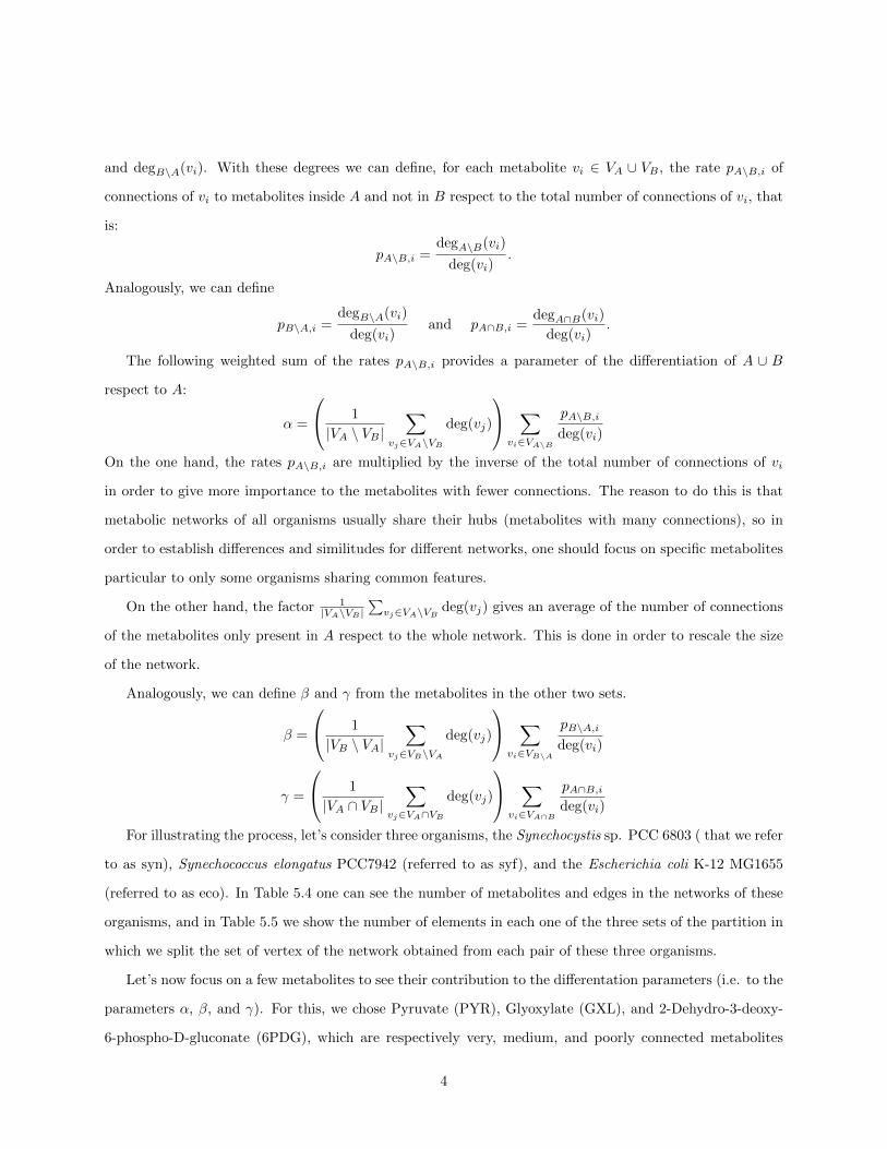
and degB\A(vi). With these degrees we can define, for each metabolite vi ∈ VA ∪ VB , the rate pA\B,i of

connections of vi to metabolites inside A and not in B respect to the total number of connections of vi, that

is:

pA\B,i =degA\B(vi)

deg(vi).

Analogously, we can define

pB\A,i =degB\A(vi)

deg(vi)and pA∩B,i =

degA∩B(vi)

deg(vi).

The following weighted sum of the rates pA\B,i provides a parameter of the differentiation of A ∪ B

respect to A:

α =

1

|VA \ VB |∑

vj∈VA\VB

deg(vj)

∑vi∈VA\B

pA\B,i

deg(vi)

On the one hand, the rates pA\B,i are multiplied by the inverse of the total number of connections of vi

in order to give more importance to the metabolites with fewer connections. The reason to do this is that

metabolic networks of all organisms usually share their hubs (metabolites with many connections), so in

order to establish differences and similitudes for different networks, one should focus on specific metabolites

particular to only some organisms sharing common features.

On the other hand, the factor 1|VA\VB |

∑vj∈VA\VB

deg(vj) gives an average of the number of connections

of the metabolites only present in A respect to the whole network. This is done in order to rescale the size

of the network.

Analogously, we can define β and γ from the metabolites in the other two sets.

β =

1

|VB \ VA|∑

vj∈VB\VA

deg(vj)

∑vi∈VB\A

pB\A,i

deg(vi)

γ =

1

|VA ∩ VB |∑

vj∈VA∩VB

deg(vj)

∑vi∈VA∩B

pA∩B,ideg(vi)

For illustrating the process, let’s consider three organisms, the Synechocystis sp. PCC 6803 ( that we refer

to as syn), Synechococcus elongatus PCC7942 (referred to as syf), and the Escherichia coli K-12 MG1655

(referred to as eco). In Table 5.4 one can see the number of metabolites and edges in the networks of these

organisms, and in Table 5.5 we show the number of elements in each one of the three sets of the partition in

which we split the set of vertex of the network obtained from each pair of these three organisms.

Let’s now focus on a few metabolites to see their contribution to the differentation parameters (i.e. to the

parameters α, β, and γ). For this, we chose Pyruvate (PYR), Glyoxylate (GXL), and 2-Dehydro-3-deoxy-

6-phospho-D-gluconate (6PDG), which are respectively very, medium, and poorly connected metabolites

4

present in these three organisms. In Table 5.6 we show the contribution of these metabolites to the parameters

α, β, and γ.

Finally, the comparison between the networks A and B, namely ζA,B , is defined as:

ζA,B =

|VB ||VA|α+ |VA|

|VB |β

2γ

The parameters α and β are balanced since some organisms have much smaller metabolic networks than

others. If this is not corrected, it results in a disproportionate size between subnetworks generated by VA\B

and by VB\A. In order to weaken this difference, the parameter factors |VB ||VA| and |VA|

|VB | are introduced. For

two identical networks, α and β are zero, and so that ζ = 0. For two networks which have not a single

metabolite in common we have γ=0 and so ζ =∞.

3 Reconstruction of the phylogenetic tree

Given a set of n organisms {A1, A2, . . . , An}, we will see how to construct their phylogenetic tree taking into

account the degrees of similarity between every pair of metabolic models.

Firstly, let N = (V,E,w) be a non-directed connected complete weighted network, where V =

{A1, A2, . . . , An} is the set of vertex that represent the metabolic models of the aforementioned organ-

isms, E is the set of edges (Ai, Aj), 1 ≤ i, j ≤ n, i 6= j, and w : E → R is a function that assigns to every

edge (Ai, Aj) the amount wi,j = ζAi,Aj. Looking at the definition of ζ, we observe that this network N must

be symmetric. In particular, all the weights in our study are strictly positive.

Secondly, we will compute a minimum spanning tree of N , that is a tree which has V as the set of vertex,

and such that the sum of the weights associated to the edges of this tree is minimum. In these trees, every

vertex Ai ∈ V is connected with at least one of the other vertex of V \ {Ai} by an edge that has minimum

weight among all the edges incident to Ai. The well-known Kruskal algorithm give us a procedure for finding

these trees, see for instance [28]. We just have to follow the trace of Kruskal algorithm in order to recover

the phylogenetic tree of the organisms represented by the models A1, . . . , An.

In order to compute the phylogenetic tree of the models {A1, A2, . . . , An}, consider the minimum spanning

tree of N , namely T = (V,E′, w|E′) where E′ ⊂ E and w|E′ denotes the restriction of the function w to the

elements in E′. Let us take all the elements of E′ in decreasing order of weights, that is E′ = {e′1, e′2, . . . , e′n−1}

with w(e′1) ≥ w(e′2) . . . ≥ w(e′1). We are going to remove edges from T following this order. Everytime an

edge is removed, the number of connected components of the resulting graph is increased in one respect to

the previous one. We can represent this division of connected componets by a binary tree. The phylogenetic

5

tree is generated taking into account how we divide T .

There are two different situations depending on the size of the (new) connected components (if any of

them consists on a single vertex or not). Let us start with the edge with maximum weight in T , that we

have denoted as e′1. Suppose that e′1 is adjacent to two vertex Ai0 and Aj0 , with 1 ≤ i0, j0 ≤ n, i 6= j. Then

two situations can happen:

(a) One of these vertex, for instance Ai0 , is a leaf (vertex of degree 1),

(b) No one of these two vertex is a leaf (each vertex is still connected with other vertex). This happens

only if the former connected component has 3 or more vertex.

We point out that our phylogenetic tree will have two types of vertex: the leaves, that represent metabolic

models, and the inner vertex, that represent that there are two branches and each one has more than one

vertex.

We start our phylogenetic tree with a vertex v0 that will be its root. Then two vertex v1, v2 are hanged

from v0. Each one of these vertex represents one of the two connected components of the network T \ {e′1}.

Let us see what to do with v1 and v2 depending in which case we are.

• If we are in case (a), one of these two vertex, for instance v1, represents the vertex Ai0 and v2 the other

one, v2, represents the other connected component of T , which is generated subgraph of T generated

by the vertex of V \ {Ai0}.

• If we are in case (b), one of the vertex, for instance v1, represents the connected component of T \{e′1}

that contains Ai0 , and the other vertex, v2, the connected component of T \ {e′1} that contains Aj0 .

This procedure is repeated again with v1 and v2 and removing e′2 from T \ {e′1}. When we remove e′2,

then either the connected component that represents v1 or v2 is split into two smaller ones, and the vertex

associated to this component plays again the role of v0. This proccess is repeated until we remove all the

edges.

Let us see how it works with two examples:

1. In Table 5.7 we have the weights associated to a set of 10 organisms. The edge of maximum weight in

the minimum spanning tree associated to the underlying network is the one that connects the mge with

the lpl, with weight 0.123. We can see in Figure 5.2 that two vertex are hanging from the root of the

tree. The one on the left represents the mge, the one on the right represents the subgraph associated

to the rest of vertex, where the lpl can be found.

6

2. In the case of 33 organisms, when we remove from the minimum spanning tree the edge with maximum

weight, we split this tree into 2 connected components: the one associated to the pair mge and mpm,

and one the associated to the other vertex.

Finally, the vertex in the phylogenetic tree can keep more information concerning the aforementioned

minimum spanning tree. Suppose that the height of our phlyogenic tree is w(e′1), that represents the

maximum of the weights in the minimum spanning tree. i.e. the weight associated to e′1. We place the root

of our phylogenetic tree at height y = w(e′1). Now, two vertex are hanged from the root. If one is associated

to a single vertex for instance v1 in case (a), then we place this vertex at height y = 0. We remember that

this vertex represents the metabolite Ai0 . If not, for instance v2 in case (a) and either v1 or v2 in case (b),

each one of these vertex represents a connected component with more than one vertex in which the minimum

spanning tree is split. In order to know at which height we should put these vertex we have to continue

removing edges from the former tree. After removing e′2, one of these connected components, for instance

the one represented by v2, is split again into 2 smaller connected components. So we place the vertex v2 at

height w(e′2). We repeat this process recursevely until the initial tree is just reduced to isolated vertex.

4 Results

We have reconstructed two phylogenetic trees, one with 10 bacteria and another one with both, prokaryotes

and eukaryotes. In Table 5.7 we show the parameter ζ for the pairwise comparison of the 10 prokaryotes in

the first tree. The data for the comparison of the 33 organisms in the second tree is given in a file in the

supplementary materials.

The organisms in each comparison are:

• 10 organisms tree → Mycoplasma genitalium (mge), Lactobacillus plantarum WCFS1 (lpl), Syne-

chocystis sp. PCC 6803 (syn), Synechococcus elongatus PCC7942 (syf), Synechococcus elongatus

PCC6301 (syc), Clostridium beijerinckii (cbe), Burkhoderia cenocepacia J2315 (bcj), Escherichia coli

K-12 MG1655 (eco), Thermotoga maritima (tma) and Yersinia pestis KIM10 (ypk).

• 33 organisms tree→ Mycoplasma genitalium (mge), Mycoplasma pneumoniae 309 (mpm), Synechocys-

tis sp. PCC 6803 (syn), Synechococcus elongatus PCC7942 (syf), Synechococcus elongatus PCC6301

(syc), Clostridium beijerinckii (cbe), Salmonella bongori (sbg), Escherichia coli K-12 MG1655 (eco),

Aquifex aeolicus (aae), Yersinia pestis KIM 10 (ypk), Cyanobacterium UCYN-A (cyu), Thermosyne-

chococcus elongatus (tel), Microcystis aeruginosa (mar), Cyanothece sp. ATCC 51142 (cyt), Cyanoth-

7

ece sp. PCC 8801 (cyp), Gloeobacter violaceus (gvi), Anabaena sp. PCC7120 (ana), Anabaena azollae

0708 (naz), Prochlorococcus marinus SS120 (pma), Trichodesmium erythraeum (ter), Acaryochloris ma-

rina (amr), Halophilic archaeon (hah), Polymorphum gilvum (pgv), Micavibrio aeruginosavorus (mai),

Agrobacterium radiobacter K84 (ara), Clostridiales genomosp. BVAB3 (clo), Gamma proteobacterium

HdN1 (gpb), Vibrio fischeri ES114 (vfi), Vibrio fischeri MJ11 (vfm), Haemophilus influenzae F3031

(hif), Coprinopsis cinerea (cci), Sus scrofa (ssc) and Leishmania braziliensis (lbz).

In Figures 5.2 and 5.3 we present the two phylogenetic trees that we have constructed.

In the first tree the only organism displaced in relation to what is expected from standard methods of

phylogenetic tree reconstruction is the tma. In both trees mge (and mpm in the second one) diverge from

other organisms at the beginning of the tree. This happens because of their minimalistic genomes, with only

a couple of hundred of metabolites in their metaboloms. As a result, when comparing with an organism

without a reduced genome with around almost a thousand metabolites, several hundred metabolites will

not have a correspondent one, increasing hugely the value of α in the calculation of the parameter ζ, and

therefore distancing these organisms from the rest. In any case, we used for the second study organisms from

very different origins in the evolutionary history and we found that the method is able to separate bacteria,

archea and eukaryotes. Different strains of the same species also appear closely related and sharing branches

with organisms from the same family and order.

We have also studied the sensibility of the parameter ζ. For this we performed a monte-carlo analysis of

ζ. The procedure for this analysis is explained as follows. Given two organisms, one of them remains the wild

type while, with the other, one builds an ensemble with Nt elements, where each element is the result of nK

knock-outs (removal of nK randomly selected reactions from the metabolic model) in the organism. Then the

calculation of ζ is performed between the wild type organism and each organism in the knock-out ensemble.

From this process one obtains an ensemble of Nt values of ζ for the comparison (one from each version of the

organism in the knock-out ensemble), from which one calculates its average and standard deviation. This

standard deviation is treated as an indicator of the sensibility of the parameter (as a function the number

of knock-outs).

We performed this sensibility analysis for four organisms (syn, syf, eco and mge) with ensembles of sizes

Nt = 500 for nK =5, 10, 50 and 100. The results are in Tables 5.8-5.11. These four organisms have been

chosen in order to observe the sensibility in the comparison between very similar organisms (syn and syf),

more distant ones (syn and eco) and very different ones (syn and mge).

8

5 Conclusions

In this work we have developed a methodology for comparing organisms based on their metabolic networks.

This methodology has been successfully applied for the reconstruction of phylogenic trees for several organ-

isms from a broad range of families and kingdoms. Resulting trees stand well their comparison with the

so-called “tree of life”. The great majority of the branches in the tree fit well their expected positions and

their distance is in good correlation with evolutionary distances. The discrepancies found can be explained

by particularities in these very few organisms not fitting the tree, such as tremendous genome reductions

that caused reduced metabolisms.

Our methodology is innovative for it is not directly based on the structure and evolution of proteins or

DNA, but on the metabolism and on the organisms’ components and metabolic capabilities, allowing one

to compare organisms very distant from the evolutionary point of view or organisms for which ortholog’s

comparison is difficult. In order to accomplish this, we make use of the correlation between evolutionary

distances and metabolic network likelihood and propose our methodology as a starting point to study it.

Metabolism information is retrieved as a subset of the whole genome information. We hereby show that

metabolic network connectivity can be used to build phylogenetic trees that are in accordance with gene-

directed trees. It can be argued whether the selected construction parameter (ζ) is the optimal one for this

purpose (or even if there is an optimal one), but it stands clear that this is an innovative application for

metabolic models, their curation and cross-species evolutionary studies.

Author’s contributions

D .Gamermann calculated the comparison coefficients and together with A. Conejero implemented the

Kruskal algorithm and reconstructed the philogenetic trees. A. Montagud analyzed the results and these

three authors contributed to the writting of the manuscript. P .F . de Cordoba and J. Urchueguıa conceived

and funded the study. All authors read and approved the manuscript.

Acknowledgements

This work has been funded by the MICINN TIN2009-12359 project ArtBioCom from the Spanish Ministerio

de Educacion y Ciencia and FP7-ENERGY-2012-1-2STAGE (Project number 308518) CyanoFactory from

the EU.

9

References1. Barrett CL, Kim TY, Kim HU, Palsson BØ, Lee SY: Systems biology as a foundation for genome-scale synthetic

biology. Current Opinion in Biotechnology 2006, 17:488–492.

2. Morange M: A new revolution? The place of systems biology and synthetic biology in the history of biology.EMBO reports 2009, 10.

3. Patil KR, Akesson M, Nielsen J: Use of genome-scale microbial models for metabolic engineering. Current opinionin Biotechnology 2004, 15:64–9.

4. Stephanopoulos G, Aristidou A, Nielsen J: Metabolic engineering: principles and methodologies. San Diego:Academic Press; 1998.

5. Nielsen J: Metabolic engineering. Applied microbiology and biotechnology 2001, 55:263–283.

6. Boghigian BA, Seth G, Kiss R, Pfeifer BA: Metabolic flux analysis and pharmaceutical production. Metabolicengineering 2010, 12:81–95.

7. Navarro E, Montagud A, Fernandez de Cordoba P, Urchueguıa JF: Metabolic flux analysis of the hydrogen pro-duction potential in Synechocystis sp. PCC6803. International Journal of Hydrogen Energy 2009, 34:8828–8838.

8. Montagud A, Navarro E, Fernandez de Cordoba P, Urchueguıa JF, Patil KR: Reconstruction and analysis ofgenome-scale metabolic model of a photosynthetic bacterium. BMC Systems Biology 2010, 4:156.

9. Montagud A, Zelezniak A, Navarro E, Fernandez de Cordoba P, Urchueguıa JF, Patil KR: Flux coupling and tran-scriptional regulation within the metabolic network of the photosynthetic bacterium Synechocystis sp. PCC6803.Biotechnology Journal 2011, 6:330–342.

10. Oberhardt MA, Palsson BØ, Papin JA: Applications of genome-scale metabolic reconstructions. Molecular sys-tems biology 2009, 5:320.

11. Edwards JS, Ramakrishna R, Schilling CH, Palsson BØ: Metabolic flux balance analysis. In Metabolic Engineer-ing. edited by Lee S, Papoutsakis E New York: Marcel Dekker Inc; 1999.

12. Angermayr SA, Hellingwerf KJ, Lindblad P, de Mattos MJT: Energy biotechnology with cyanobacteria. CurrentOpinion in Biotechnology 2009, 20:257–63.

13. Nevoigt E (2008) Progress in metabolic engineering of Saccharomyces cerevisiae. Microbiol Mol Biol Rev 72:379–412

14. Stolyar S,Van Dien S, Hillesland KL, Pinel N, Lie TJ, Leigh JA, StahlDA (2007) Metabolic modeling of amutualistic microbial community. Mol Syst Biol 3: 92

15. Guimera R, Nunes Amaral LA: Functional cartography of complex metabolic networks. Nature 2005, 433:895–900.

16. Yang Z, Rannala B: Molecular phylogenetics: principles and practice. Nature reviews. Genetics 2012, 13:303–14.

17. Maser, P. et al. Phylogenetic relationships within cation transporter families of Arabidopsis. Plant Physiol. 126,1646–1667 (2001).

18. Edwards, S. V. Is a new and general theory of molecular systematics emerging? Evolution 63, 1–19 (2009)

19. Marra, M. A. et al. The genome sequence of the SARS-associated coronavirus. Science 300, 1399–1404 (2003).

20. Grenfell, B. T. et al. Unifying the epidemiological and evolutionary dynamics of pathogens. Science 303, 327–332(2004).

21. Salipante, S. J. Horwitz, M. S. Phylogenetic fate mapping. Proc. Natl Acad. Sci. USA 103, 5448–5453 (2006).

22. Gray, R. D., Drummond, A. J. Greenhill, S. J. Language phylogenies reveal expansion pulses and pauses in pacificsettlement. Science 323, 479–483 (2009).

23. Brady, A., Salzberg, S. PhymmBL expanded: confidence scores, custom databases, parallelization and more.Nature Methods 8, 367 (2011).

24. Kellis, M., Patterson, N., Endrizzi, M., Birren, B., Lander, E. S. Sequencing and comparison of yeast species toidentify genes and regulatory elements. Nature 423, 241–254 (2003).

25. Green, R. E. et al. A draft sequence of the Neandertal genome. Science 328, 710–722 (2010).)

26. R. Reyes, D. Gamermann, A. Montagud, D. Fuente, J. Triana, J. F. Urchuegıa, P. Fernandez deCordoba. Automation on the generation of genome scale metabolic models. arXiv:1206.0616v1 [q-bio.MN](http://arxiv.org/abs/1206.0616v1). Journal of computational biology (2012) in print.

27. M. Kanehisa and S. Goto. KEGG: Kyoto encyclopedia of genes and genomes. Nucleic acids res. 28, 27-30 (2000).

28. J.L. Gross and J. Yellen, Graph theory and its applications. Boca Raton: Chapman & Hall/CRC; 2006.

10

Figures5.1 Figure 1 - conjs.pdf

A B

A B

A B

A B

(Color on-line) Representation of the sets of metabolites between two organisms.

5.2 Figure 2 - tree10.png

(Color on-line) Phylogenetic tree with 10 organisms.

11

5.3 Figure 3 - tree30.png

(Color on-line) Phylogenetic tree with 33 organisms.

Tables5.4 Table 1 - Vertex and edges in the networks of syn, syf and eco.

Organism # Vertex # Edgessyn 1001 2891syf 979 2810eco 1227 3801

5.5 Table 2 - Metabolites in the three sets of the partition when comparing three organisms.syf eco

|VA ∩ VB | = 911 |VA ∩ VB | = 778syn |VA \ VB | = 90 |VA \ VB | = 223

|VB \ VA| = 68 |VB \ VA| = 449- |VA ∩ VB | = 775

syf - |VA \ VB | = 204- |VB \ VA| = 452

12

5.6 Table 3 - Contribution of different metabolites to the differentiation parameter (ζ) between twonetworks. The column δi shows the weight of the metabolite in the calculation of pA∩B,i which isthe inverse of the degree of the metabolite divided by the sum of the inverses of the degrees ofall metabolites contributing to the parameter.

Metabolite Organisms in pA∩B,i δi Contribution (%)comparison

syn and syf 0.98 0.127 0.0064PYR syn and eco 0.73 0.117 0.0044

syf and eco 0.75 0.113 0.0044syn and syf 0.86 0.454 0.020

GXL syn and eco 0.87 0.550 0.024syf and eco 0.80 0.439 0.018syn and syf 1.00 3.176 0.16

6PDG syn and eco 0.80 1.762 0.072syf and eco 0.80 1.757 0.072

5.7 Table 4 - Comparison matrix for ten organisms.org mge lpl syn syf syc cbe bcj eco tma ypk

mge 0.0 0.123 0.1951 0.1753 0.1906 0.1438 0.1374 0.1384 0.1306 0.1384lpl 0.123 0.0 0.1554 0.1543 0.1645 0.0719 0.1217 0.1227 0.0716 0.1154syn 0.1951 0.1554 0.0 0.0195 0.0188 0.1286 0.1135 0.1137 0.1687 0.1248syf 0.1753 0.1543 0.0195 0.0 0.0054 0.1262 0.117 0.1076 0.1677 0.1174syc 0.1906 0.1645 0.0188 0.0054 0.0 0.1327 0.1149 0.1043 0.1657 0.1133cbe 0.1438 0.0719 0.1286 0.1262 0.1327 0.0 0.1121 0.0933 0.0737 0.1071bcj 0.1374 0.1217 0.1135 0.117 0.1149 0.1121 0.0 0.0678 0.1324 0.068eco 0.1384 0.1227 0.1137 0.1076 0.1043 0.0933 0.0678 0.0 0.1101 0.0295tma 0.1306 0.0716 0.1687 0.1677 0.1657 0.0737 0.1324 0.1101 0.0 0.1075ypk 0.1384 0.1154 0.1248 0.1174 0.1133 0.1071 0.068 0.0295 0.1075 0.0

5.8 Table 5 - Sensibility calculation for Nt = 500 and nK = 5. Each element in the table is the averageof the parameter ζ in an ensemble plus (minus) its standard deviation (ζ ± σζ).

org / org syn syf eco mgesyn 0.0002 ± 0.0003 0.0184 ± 0.0005 0.0893 ± 0.0005 0.1600 ± 0.0014syf 0.0184 ± 0.0004 0.0002 ± 0.0003 0.0857 ± 0.0006 0.1527 ± 0.0014eco 0.0892 ± 0.0005 0.0856 ± 0.0005 0.0001 ± 0.0002 0.1278 ± 0.0009mge 0.1597 ± 0.0025 0.1527 ± 0.0026 0.1283 ± 0.0015 0.0014 ± 0.0016

5.9 Table 6 - Sensibility calculation for Nt = 500 and nK = 10. Each element in the table is theaverage of the parameter ζ in an ensemble plus (minus) its standard deviation (ζ ± σζ).


13





Additional FilesAdditional file 1 - comps 33orgs.dat

Table with the parameter ζ resulting from the comparison of 33 organisms.

14

gamermann, d.; montagud aquino, a.; conejero casares, ja

Documents