garch modeling by lars karlsson - analytical financejanroman.dhis.org/finance/volatility...
TRANSCRIPT
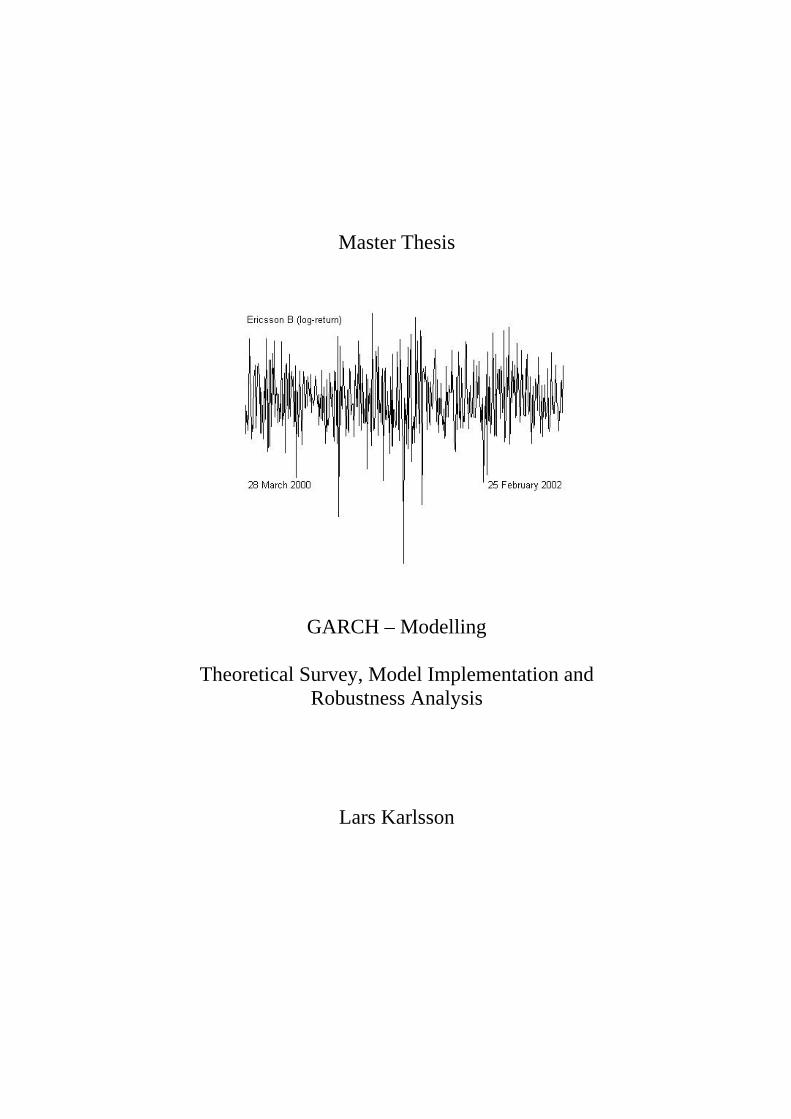
Master Thesis
GARCH – Modelling
Theoretical Survey, Model Implementation and Robustness Analysis
Lars Karlsson

2
3
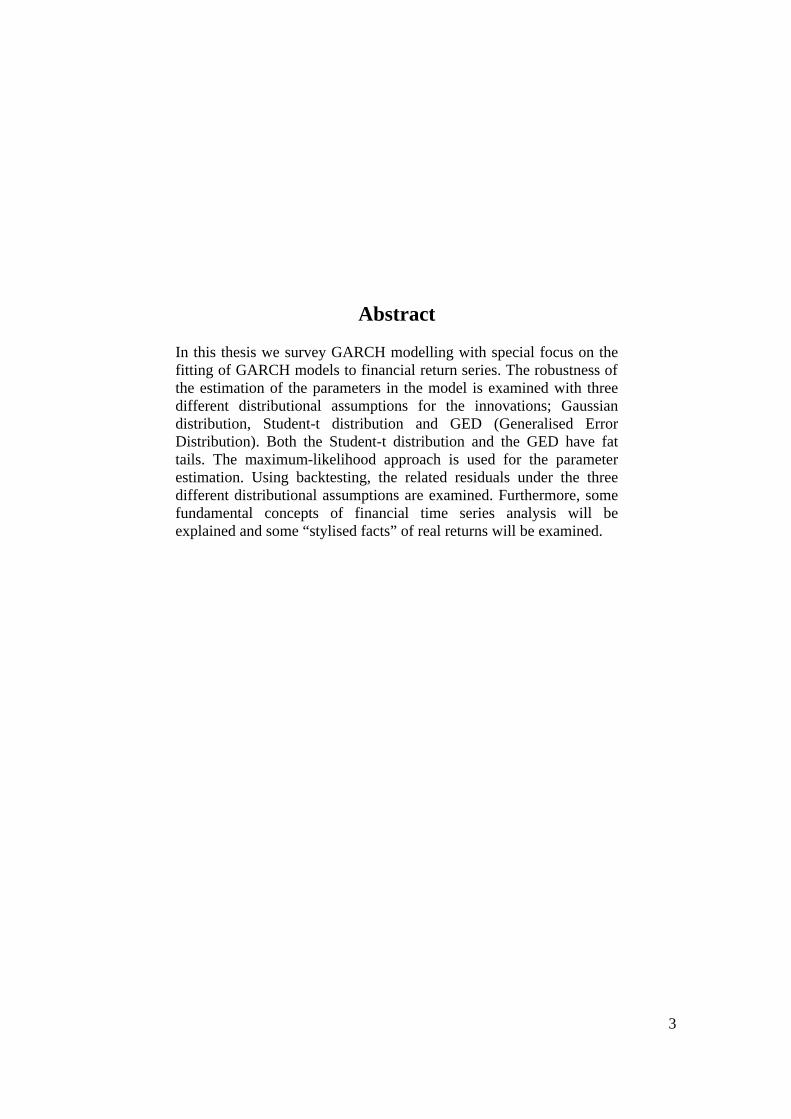
Abstract
In this thesis we survey GARCH modelling with special focus on the fitting of GARCH models to financial return series. The robustness of the estimation of the parameters in the model is examined with three different distributional assumptions for the innovations; Gaussian distribution, Student-t distribution and GED (Generalised Error Distribution). Both the Student-t distribution and the GED have fat tails. The maximum-likelihood approach is used for the parameter estimation. Using backtesting, the related residuals under the three different distributional assumptions are examined. Furthermore, some fundamental concepts of financial time series analysis will be explained and some “stylised facts” of real returns will be examined.
4
Acknowledgements I would like to thank Peter Alaton and Robert Thorén at Algorithmica Research AB for giving me the opportunity of doing this thesis and for their help and contributions with real-world financial knowledge. I also would like to thank Professor Boualem Djehiche and Senior Lecturer Jan Enger, as well as Henrik Hult, at the Department of Mathematical Statistics at the Royal Institute of Technology (KTH) for their important guidance and valuable remarks. Finally, I would like to thank my family and girlfriend for their support during the whole project. Especially, I would like to express my deepest gratitude to my mother and sister for their endless love, support and encouragement.
5
Contents 1 Introduction . . . . . . . . . . . . . . . . . . . . . . . . . . . . . . . . . . . . . . . . . . . . . . . . . . . . .7 2 Financial Time Series . . . . . . . . . . . . . . . . . . . . . . . . . . . . . . . . . . . . . . . . . . . . . 8
2.1 Empirical Properties 9 2.1.1 Kurtosis 9 2.1.2 Autocorrelation 11 2.1.3 Power Law Tails 12 2.1.4 Skewness 12 2.1.5 Holiday Effect 13
3 “Stylised Facts” About Financial Data . . . . . . . . . . . . . . . . . . . . . . . . . . . . . . 14 4 Stochastic Volatility Models . . . . . . . . . . . . . . . . . . . . . . . . . . . . . . . . . . . . . . . 16 5 The GARCH Family . . . . . . . . . . . . . . . . . . . . . . . . . . . . . . . . . . . . . . . . . . . . . 18
5.1 Symmetric GARCH Models 18 5.1.1 GARCH 18 5.1.2 IGARCH 19
5.2 Asymmetric GARCH Models 20 5.2.1 EGARCH 20 5.2.2 GJR-GARCH 21 5.2.3 APARCH 22
6 Parameter Estimation in the GARCH Model . . . . . . . . . . . . . . . . . . . . . . . . 23 6.1 Maximum-Likelihood Estimation (MLE) 23
6.1.1 Stationarity 23 6.1.2 Gaussian Quasi Maximum-Likelihood Estimation 25 6.1.3 Fat-Tailed Maximum-Likelihood Estimation 26
6.2 Distributions 27 6.2.1 Normal Distribution 27 6.2.2 Student-t Distribution 27 6.2.3 Generalised Error Distribution (GED) 28
7 Robustness of Estimation . . . . . . . . . . . . . . . . . . . . . . . . . . . . . . . . . . . . . . . . . 29 7.1 Residuals 29 7.2 Robustness of MLE on Simulated Data 31
7.2.1 Examples With Simulated Data 32 7.2.2 Conclusion of Examples 38
7.3 Robustness of MLE on Empirical Data 39 7.3.1 Example With Empirical Data 39 7.3.2 Conclusion of Empirical Example 44
7.4 Maximum-Likelihood Value Comparison 45 7.4.1 Conclusion Maximum-Likelihood Value Comparison 45
6
8 Variance Forecasting . . . . . . . . . . . . . . . . . . . . . . . . . . . . . . . . . . . . . . . . . . . . 46 8.1 GARCH(1,1) 46 8.2 IGARCH(p,q) 48
9 Multivariate GARCH Models . . . . . . . . . . . . . . . . . . . . . . . . . . . . . . . . . . . . . 48 10 Appendix A . . . . . . . . . . . . . . . . . . . . . . . . . . . . . . . . . . . . . . . . . . . . . . . . . . . . 49
10.1 Stationarity 49 10.2 Proof of Corollary 49
11 References . . . . . . . . . . . . . . . . . . . . . . . . . . . . . . . . . . . . . . . . . . . . . . . . . . . . . 50
7
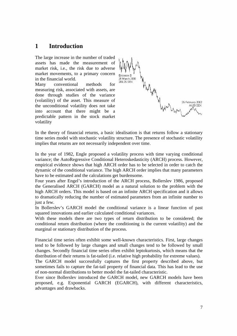
1 Introduction The large increase in the number of traded assets has made the measurement of market risk, i.e., the risk due to adverse market movements, to a primary concern in the financial world. Many conventional methods for measuring risk, associated with assets, are done through studies of the variance (volatility) of the asset. This measure of the unconditional volatility does not take into account that there might be a predictable pattern in the stock market volatility In the theory of financial returns, a basic idealisation is that returns follow a stationary time series model with stochastic volatility structure. The presence of stochastic volatility implies that returns are not necessarily independent over time. In the year of 1982, Engle proposed a volatility process with time varying conditional variance; the AutoRegressive Conditional Heteroskedasticity (ARCH) process. However, empirical evidence shows that high ARCH order has to be selected in order to catch the dynamic of the conditional variance. The high ARCH order implies that many parameters have to be estimated and the calculations get burdensome. Four years after Engel’s introduction of the ARCH process, Bollerslev 1986, proposed the Generalised ARCH (GARCH) model as a natural solution to the problem with the high ARCH orders. This model is based on an infinite ARCH specification and it allows to dramatically reducing the number of estimated parameters from an infinite number to just a few. In Bollerslev’s GARCH model the conditional variance is a linear function of past squared innovations and earlier calculated conditional variances. With these models there are two types of return distribution to be considered; the conditional return distribution (where the conditioning is the current volatility) and the marginal or stationary distribution of the process. Financial time series often exhibit some well-known characteristics. First, large changes tend to be followed by large changes and small changes tend to be followed by small changes. Secondly financial time series often exhibit leptokurtosis, which means that the distribution of their returns is fat-tailed (i.e. relative high probability for extreme values). The GARCH model successfully captures the first property described above, but sometimes fails to capture the fat-tail property of financial data. This has lead to the use of non-normal distributions to better model the fat-tailed characteristic. Ever since Bollerslev introduced the GARCH model, new GARCH models have been proposed, e.g. Exponential GARCH (EGARCH), with different characteristics, advantages and drawbacks.
8
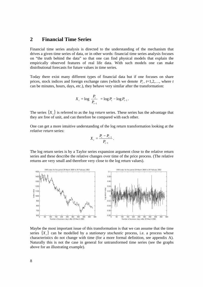
2 Financial Time Series Financial time series analysis is directed to the understanding of the mechanism that drives a given time series of data, or in other words: financial time series analysis focuses on “the truth behind the data” so that one can find physical models that explain the empirically observed features of real life data. With such models one can make distributional forecasts for future values in time series. Today there exist many different types of financial data but if one focuses on share prices, stock indices and foreign exchange rates (which we denote tP , t=1,2,…, where t can be minutes, hours, days, etc.), they behave very similar after the transformation:
11
logloglog −−
−=
= tt
t
tt PP
PP
X .
The series { }tX is referred to as the log return series. These series has the advantage that they are free of unit, and can therefore be compared with each other. One can get a more intuitive understanding of the log return transformation looking at the relative return series:
1
1
−
−−=
t
ttt P
PPX .
The log return series is by a Taylor series expansion argument close to the relative return series and these describe the relative changes over time of the price process. (The relative returns are very small and therefore very close to the log return values).
Maybe the most important issue of this transformation is that we can assume that the time series { }tX can be modelled by a stationary stochastic process, i.e. a process whose characteristics do not change with time (for a more formal definition, see appendix A). Naturally this is not the case in general for untransformed time series (see the graphs above for an illustrating example).
9
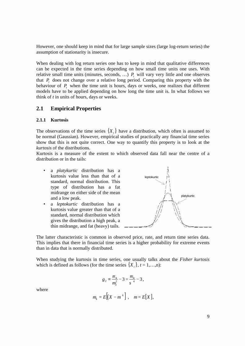
However, one should keep in mind that for large sample sizes (large log-return series) the assumption of stationarity is insecure. When dealing with log return series one has to keep in mind that qualitative differences can be expected in the time series depending on how small time units one uses. With relative small time units (minutes, seconds, …) tP will vary very little and one observes that tP does not change over a relative long period. Comparing this property with the behaviour of tP when the time unit is hours, days or weeks, one realizes that different models have to be applied depending on how long the time unit is. In what follows we think of t in units of hours, days or weeks. 2.1 Empirical Properties 2.1.1 Kurtosis The observations of the time series { }tX have a distribution, which often is assumed to be normal (Gaussian). However, empirical studies of practically any financial time series show that this is not quite correct. One way to quantify this property is to look at the kurtosis of the distributions. Kurtosis is a measure of the extent to which observed data fall near the centre of a distribution or in the tails:
• a platykurtic distribution has a kurtosis value less than that of a standard, normal distribution. This type of distribution has a fat midrange on either side of the mean and a low peak.
• a leptokurtic distribution has a kurtosis value greater than that of a standard, normal distribution which gives the distribution a high peak, a thin midrange, and fat (heavy) tails.
The latter characteristic is common in observed price, rate, and return time series data. This implies that there in financial time series is a higher probability for extreme events than in data that is normally distributed. When studying the kurtosis in time series, one usually talks about the Fisher kurtosis which is defined as follows (for the time series { }tX , t = 1,…,n):
33 44
22
42 −=−≡
σµ
µµ
γ ,
where
( )[ ] [ ]XEXE kk =−= µµµ , ,
leptokurtic
platykurtic
10
is the central moment of degree k. This kurtosis measure exists only if the fourth moment exists and is finite. Kurtosis is a normalized form of the fourth central moment of a distribution. In the Fisher kurtosis the digit three is subtracted to give the normal distribution the kurtosis zero (the distribution is mesokurtic). Supposing that
)1,0(~ NX t , the fourth and second central moments are given by:
[ ] [ ] 3e21
)( 2t-4444
2
===−= ∫∞
∞−
dttXEXEπ
µµ
[ ] 1)()( 22 ==−= XVarXE µµ
which shows that the Fisher kurtosis for normal distributions is zero. The central moment of degree k is estimated with:
( )∑=
−=n
i
kik xx
n 1
1µ .
In the cases above we have the following definitions:
• platykurtic distributions: 02 <γ • leptokurtic distributions: 02 >γ (excess kurtosis) • mesokurtic distributions: 02 =γ
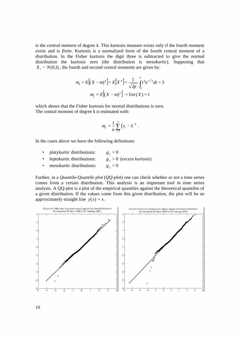
Further, in a Quantile-Quantile plot (QQ-plot) one can check whether or not a time series comes from a certain distribution. This analysis is an important tool in time series analysis. A QQ-plot is a plot of the empirical quantiles against the theoretical quantiles of a given distribution. If the values come from this given distribution, the plot will be an approximately straight line xxy =)( .
11
This is a visual method of analysis where the analyser can get a better knowledge of the empirical distribution and its deviations from a theoretical distribution. 2.1.2 Autocorrelation One important tool for assessing the degree of dependence in observed data is the sample autocorrelation function (sample ACF) of the data. First some definitions:
• Let nxx ,...,1 be observations of a time series. The sample mean of nxx ,...,1 is
∑=
=n
ttx
nx
1
1.
• The sample autocovariance function is:
nhnxxxxn
h t
hn
tht <<−−−≡ ∑
−
=+ ),)((
1)(ˆ
||
1||γ ,
where ),(Cov)( thtX XXh +=γ .
• The sample autocorrelation function is:
nhnh
h <<−= ,)0(ˆ)(ˆ
)(ˆγγ
ρ .
A typical feature of financial time series is the structure of the autocorrelation function; the sample autocorrelations are negligible at almost all lags, i.e., the assumption of { }tX being white noise feels quite natural, but the sample autocorrelations of the squares or absolute values are different for a large number of lags and stay almost constant and positive for large lags. There are different opinions of how this property is to be interpreted and the most common idea is to interpret the slow decaying lags as a long-term memory or long-range dependence (LRD). Although some opponents claim that this might not be right due to non-existence of fourth moments, which implies that the ACF does not produce anything meaningful, and secondly due to non-stationary effects. Definition: Long-Range Dependence { }tX is said to exhibit long-range dependence if
∞=∑∞
=
|)(|0h
X hρ .
12
fat-tailed distribution
normal distribution
Why bother looking at the absolute and squared log-returns? One reason is that empirical evidence shows that the sequence of the signs of a log-return series has similar statistical properties as a sequence of i.i.d. (independent, identically distributed) symmetric Bernoulli random variables. Therefore numerous models are of the form
)(|| ttt XsignXX = , where the sequence { })( tXsign consists of i.i.d. symmetric Bernoulli random variables, and so one is left to model absolute returns. Various popular models, for example GARCH models, are of the form ttt ZX σ= (see chapter 3), where { }tZ is an i.i.d. symmetric sequence, the volatility process { }tσ is stationary and non-negative, and tZ and tσ are independent for every fixed t. Thus, the sequence { } { })()( tt ZsignXsign = is i.i.d. Bernoulli, as desired. What one is interested in is the volatility of the log-return, but by its construction, it cannot be observed. Therefore the observable quantities | tX | and 2
tX often are considered as surrogate values or “estimators” of tσ and 2
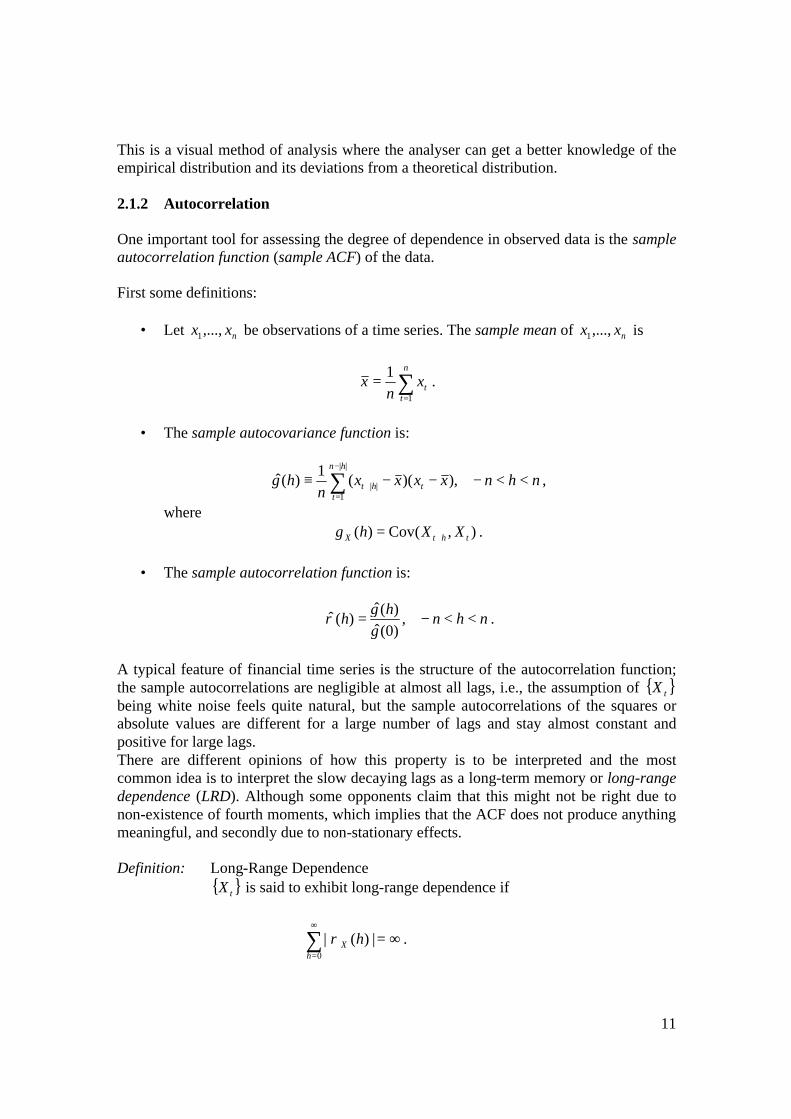
tσ respectively and that is why they sometimes are in focus. 2.1.3 Power Law Tails Log-return data of financial time series often exhibits heavy-tailed distributions. Conveniently, these tails can be modelled with distributions with power law tails, i.e., for large x and some positive number α (the tail index),
α−
∞→=
>>
xuXPxuXP
u )()(
lim .
Examples of distributions satisfying this tail condition are for example the Pareto distribution (with an exact power law) and the Student-t distribution with α degrees of freedom. In this thesis the Student-t distribution is considered. 2.1.4 Skewness Observations of the empirical distribution of { }tX often show that the distribution is leptokurtic. Another property that deviates from the so often assumed Gaussian distribution is that the empirical distribution is not symmetric. Skewness defines the degree of asymmetry of a distribution and several types of skewness are defined. The Fisher skewness (the most common type of skewness, usually referred to simply as skewness) is defined by:
33
232
31 σ
µµµ
γ =≡ ,
where 3µ is the third central moment, and 2/1
2µ is the standard deviation. A negative skewness value indicates that the data has a distribution skewed to the left. This means that the left tail is heavier than the right tail in the distribution. Respectively, a positive skewness value indicates a right skewed distribution with a right tail heavier than its left tail. In this thesis the skewness of the time series is neglected.
13
2.1.5 Holiday Effect During weekends and holidays information accumulates. This could be reflected in prices when the markets reopen. If the information stream assumes to be constant, the variance of the returns over the period from Friday close to the Monday close should be three times the variance from the Monday close to the Tuesday close. However, the assumption of constant information stream is not in accordance to the real life experience. The information rate during weekends and holidays is lower than during working days, which reduces the holiday effect. This property is also neglected in this thesis.
14
3 “Stylised Facts” About Financial Data The log-returns ( 1loglog −−= ttt PPX ) of share prices, stock indices and foreign exchange rates tP , ,...2,1=t , often show the following features:
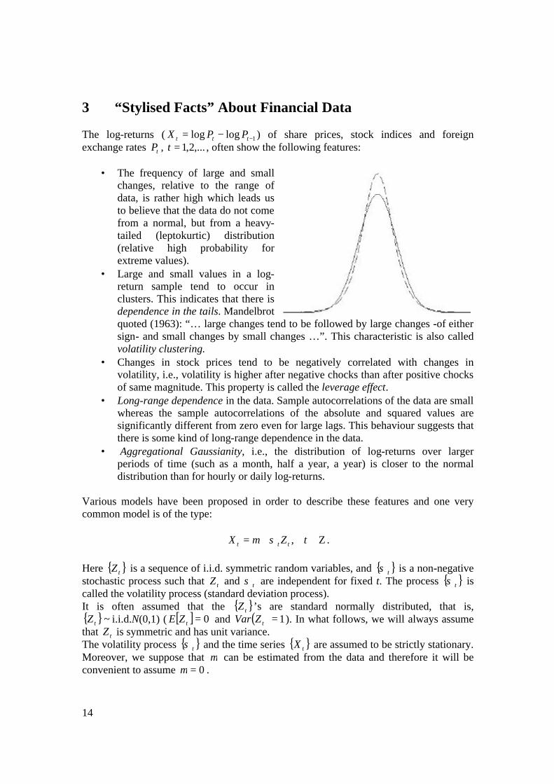
• The frequency of large and small changes, relative to the range of data, is rather high which leads us to believe that the data do not come from a normal, but from a heavy-tailed (leptokurtic) distribution (relative high probability for extreme values).
• Large and small values in a log-return sample tend to occur in clusters. This indicates that there is dependence in the tails. Mandelbrot quoted (1963): “… large changes tend to be followed by large changes -of either sign- and small changes by small changes …”. This characteristic is also called volatility clustering.
• Changes in stock prices tend to be negatively correlated with changes in volatility, i.e., volatility is higher after negative chocks than after positive chocks of same magnitude. This property is called the leverage effect.
• Long-range dependence in the data. Sample autocorrelations of the data are small whereas the sample autocorrelations of the absolute and squared values are significantly different from zero even for large lags. This behaviour suggests that there is some kind of long-range dependence in the data.
• Aggregational Gaussianity, i.e., the distribution of log-returns over larger periods of time (such as a month, half a year, a year) is closer to the normal distribution than for hourly or daily log-returns.
Various models have been proposed in order to describe these features and one very common model is of the type:
Ζ∈+= tZX ttt ,σµ . Here { }tZ is a sequence of i.i.d. symmetric random variables, and { }tσ is a non-negative stochastic process such that tZ and tσ are independent for fixed t. The process { }tσ is called the volatility process (standard deviation process). It is often assumed that the { }tZ ’s are standard normally distributed, that is, { }~tZ i.i.d.N(0,1) ( [ ] 0=tZE and ( ) 1=tZVar ). In what follows, we will always assume that tZ is symmetric and has unit variance. The volatility process { }tσ and the time series { }tX are assumed to be strictly stationary. Moreover, we suppose that µ can be estimated from the data and therefore it will be convenient to assume 0=µ .
15
There are various reasons for this particular choice of model:
• the direction of the price changes is modelled only by the sign of tZ , independently of the order of magnitude of this change, which is directed by the volatility tσ . This is in agreement with the empirical observation that it is difficult, or even impossible, to predict the sign of price changes.
• since tσ and tZ are independent, and tZ is assumed to have mean zero and variance 1, 2
tσ is then the conditional variance of tX given tσ .
( ) [ ] [ ]( ) [ ] [ ]( ) =−=−= 22222tttttttttttt ZEZEXEXEXVar σσσσσσσ
[ ] [ ] [ ] [ ]( ) [ ] 22222ttttttttttt EZEEZEE σσσσσσσσσ ==−= .
16
4 Stochastic Volatility Models As shown in the previous chapter, most models for financial returns are of the form:
Ζ∈= tZX ttt ,σ ,
where { }tZ is a sequence of i.i.d. symmetric random variables, and { }tσ is a non-negative stochastic process such that tZ and tσ are independent for fixed t. There is strong empirical support for stochastic volatility in financial time series and the presence of stochastic volatility implies that returns are not necessarily independent over time. The standard assumption for the noise tZ is that { }~tZ i.i.d. )1,0(N with { }tZ independent of the standard deviation process { }tσ . Volatility is a central part of most asset pricing models. In these models, one often assumes that the volatility is constant over time. However, it is well known that financial time series exhibit time-varying volatility. In the year of 1982, Engle [6] proposed a model for { }tσ :
2
10
2it
p
iit X −
=∑+= αασ .
This model is called the AutoRegressive Conditional Heteroskedasticity (ARCH process) where the “autoregressive” property in principle means that old events leave waves behind a certain time after the actual time of the action. The process depends on its past. The terms “conditional heteroskedasticity” means that the variance (conditional on the available information) varies and depends on old values of the process. One can resemble this with the process having a short-term memory and that the behaviour of the process is influenced by this memory. However, since it can expected that 2
tσ is a time-changing weighted average of past squared observations, it is quite natural to define 2
tσ , not only as a weighted average of past 2
tX ’s, but also of past 2tσ . Empirical evidence shows that high ARCH order has to
be selected in order to catch the dynamic of the conditional variance. This leads to the Generalised ARCH model (GARCH) introduced 1986 by Bollerslev [1]. The volatility process is:
∑∑=
−−=
++=q
jjtjit
p
iit X
1
22
10
2 σβαασ ,
where the iα ’s and the jβ ’s are non-negative parameters. This model reduces the number of estimated parameters from infinitely many to only just a few. (One can easily see that the GARCH model is based on an infinite ARCH specification. See derivation in chapter 5.1.1)

17
GARCH has gained fast acceptance and popularity in the financial world. This can be explained by various arguments:
• the GARCH process has a close relation to ARMA processes. This suggests that the theory behind the GARCH process might be closely related to the theory of ARMA processes, which is well studied and widely known.
• one can get a reasonable good fit to real life financial data even with a GARCH(1,1) model with only three parameters, provided that the sample is not too long so that the stationary assumption is unreliable.
In the following chapter a survey of some different GARCH models is done.
18
5 The GARCH Family Ever since Bollerslev introduced the GARCH(p,q)-model, new models with different characteristics have been invented. The existing models can be divided into two main categories: symmetric and asymmetric models. In the symmetric models, the conditional variance only depends on the magnitude, and not the sign, of the underlying asset tX . This property is seldom in accordance with empirical results where a leverage effect often is present, i.e., volatility increases more after negative return shocks than after positive return shocks of the same magnitude (“bad news” generates higher volatility more than “good news” lowers the volatility). However, in the asymmetric models these characteristics are more or less captured. All the following models build on the multiplicative form ttt ZX σ= , Ζ∈t for the financial log-returns (as shown earlier). The standard assumption for the noise is that { }tZ is i.i.d. symmetric random variables with zero mean and unit variance. The volatility process { }tσ is a non-negative stochastic process such that tZ and tσ are independent for fixed t. 5.1 Symmetric GARCH Models 5.1.1 GARCH Let tX denote a real-valued discrete-time stochastic process. The GARCH(p,q) process proposed by Bollerslev is then given by:
∑∑=
−−=
++=q
jjtjit
p
iit
ttt
X
NX
1
22
10
2
2 ),0(~|
σβαασ
σσ
qj
piqp
j
i
,...,1,0
,...,1,0,00,0
0
=≥=≥>
≥>
βαα
or, using the lag or backshift operator B defined as B tX = 1−tX , the GARCH(p,q) model is:
220
2 )()( ttt BXB σβαασ ++= , with p
p zzzz αααα +++= ...)( 221 and q
q zzzz ββββ +++= ...)( 221 . For q=0 the
process reduces to the ARCH(p) process, and for p=q=0 tX is simply white noise. The GARCH(p,q) process with an i.i.d. noise sequence { }tZ such that [ ] 12 =tZE and
[ ] 0=tZE , is strictly stationary with finite variance if (see chapter 6.1.1):
19
00 >α and 111
<+ ∑∑==
q
jj
p
ii βα .
The GARCH process has a close relation to ARMA processes. By rearranging the GARCH(p,q) model defining 22
ttt X συ −≡ , it follows that:
( ) tttt BXBBX υυββαα +−++= −− 12
102 )()()( ,
which defines an ARMA(max(p,q),p) model for 2
tX . This relation to ARMA processes suggests that the theory behind the GARCH processes might be closely related to ARMA process theory, which is quite easy and widely known. Although, one has to be careful because the noise sequence { }tσ depends on the tX ’s themselves, so that a complicated non-linear relationship of the tX ’s is built up. Furthermore, it is easy to see that the GARCH model is based on an infinite ARCH specification. If all the roots of the polynomial 0)(1 =− Bβ lie outside the unit circle, we get: ( ) 2
02 )()(1 tt XBB αασβ +=− , or equivalently:
2
11
0202
...1)(1)(
)1(1 iti
iq
tt XXB
B−
∞
=∑+
−−−=
−+
−= λ
ββα
βα
βα
σ ,
where the ?i’s are suitable constants which together with ),0(~| 2
ttt NX σσ may be seen as an ARCH( ∞ ) process. 5.1.2 IGARCH When estimating the parameters in the GARCH model one often observes that the sum of the parameters is close to one. For the parameter setting:
111
=+ ∑∑==
q
jj
p
ii βα .
Engle and Bollerslev coined the name Integrated GARCH (IGARCH). Here, the “integrated” refers to the fact that there might be a unit root problem which could lead to the non-existence of a stationary version of { }tX (it has infinite variance). However, this is not the case for the IGARCH under the conditions of Theorem in chapter 6.1.1 plus some mild additional assumptions (see [10] for further information). Thus, the IGARCH has a strictly stationary solution, but with infinite variance. To see this we take the expectations of the conditional variance and observe that E[ 2
tX ] = E[ 2tσ ] which gives:
[ ] [ ] [ ] ( ) [ ]20
220
2 )1()1()()( tttt EEBXEBE σβαασβαασ ++=++= .
20
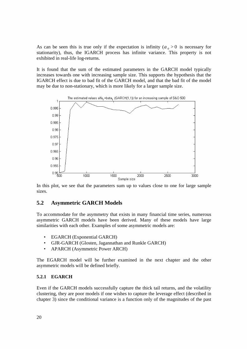
As can be seen this is true only if the expectation is infinity ( 00 >α is necessary for stationarity), thus, the IGARCH process has infinite variance. This property is not exhibited in real-life log-returns. It is found that the sum of the estimated parameters in the GARCH model typically increases towards one with increasing sample size. This supports the hypothesis that the IGARCH effect is due to bad fit of the GARCH model, and that the bad fit of the model may be due to non-stationary, which is more likely for a larger sample size.
In this plot, we see that the parameters sum up to values close to one for large sample sizes. 5.2 Asymmetric GARCH Models To accommodate for the asymmetry that exists in many financial time series, numerous asymmetric GARCH models have been derived. Many of these models have large similarities with each other. Examples of some asymmetric models are:
• EGARCH (Exponential GARCH) • GJR-GARCH (Glosten, Jagannathan and Runkle GARCH) • APARCH (Asymmetric Power ARCH)
The EGARCH model will be further examined in the next chapter and the other asymmetric models will be defined briefly. 5.2.1 EGARCH Even if the GARCH models successfully capture the thick tail returns, and the volatility clustering, they are poor models if one wishes to capture the leverage effect (described in chapter 3) since the conditional variance is a function only of the magnitudes of the past
21
values and not their sign. The conditional variance 2tσ of tX given information at time t,
obviously must be non-negative with probability one. In GARCH models this property is assured by making 2
tσ a linear combination (with positive weights) of positive random variables (as in the GARCH(p,q) case). Another way of making 2
tσ non-negative is by making ( )2ln tσ linear in some function of time and lagged tZ ’s. This formulation leads to the asymmetric GARCH model, Exponential GARCH, of Nelson (1991) [7]:
( ) ( )2
11-it0
2 lnZ)ln( jt
q
jj
p
iit g −
==∑∑ ++= σβαασ .
The value of )( tZg depends on several elements. Nelson notes, “to accommodate the asymmetric relation between stock returns and volatility changes, the value of )( tZg must be a function of both the magnitude and the sign of tZ .” This leads to following representation:
{ [ ][ ]44 344 21effect magnitude
2
effectsign
1 ||||)( tttt ZEZZZg −+= θθ .
With this construction, { } ∞−∞= ,)( ttZg is a zero-mean, i.i.d. random sequence. (Each component has mean zero.) Over the range ∞<< tZ0 , )( tZg is linear in tZ with slope
21 θθ + , and over the range 0≤<∞− tZ , )( tZg is linear with slope 21 θθ − . Thus )( tZg allows the conditional variance 2
tσ to respond asymmetrically to rises and falls in stock price. To see that the term [ ][ ]||||2 tt ZEZ −θ represents the magnitude effect one first assumes that 01 =θ and 02 >θ . This makes the innovation in )ln( 2
1+tσ positive (negative) when the magnitude of tZ is larger (smaller) than its expected value. Assuming that 01 <θ and
02 =θ . The innovation in conditional variance is now positive (negative) when returns innovations are negative (positive). In contrast to the GARCH models, the EGARCH models do not have any restrictions on the parameters in the model. The EGARCH model always produces a positive conditional variance independently of the signs of the estimated parameters in the model and no restrictions are needed. This is preferable when the restrictions in the GARCH model sometimes create problems when estimated parameters violate the inequality constraints. 5.2.2 GJR-GARCH GJR-GARCH (Glosten, Jagannathan and Runkle GARCH):
( )
≥<
=
+++=
−
−==
−−−− ∑∑
0when1
0when0
2
11
220
2
t
tt
jt
q
jj
p
iititiitit
X
XS
XSX σβωαασ
22
In this model it is supposed that the effect of the 2tX on the conditional variance 2
tσ is different accordingly to the sign of tX and this is why the variable −
tS is introduced. This implies that the model accommodates the leverage effect. 5.2.5 APARCH APARCH (Asymmetric Power ARCH):
( )
pi
qjpi
XX
i
j
i
jt
p
i
q
jjitiitit
,..,111
,...,10,...,10
0 ,0
||
0
1 10
=<<−
=≥=≥≥>
+−+= −= =
−−∑ ∑
γ
βα
δα
σβγαασ δδδ
Most of the GARCH models are non-nested (they can not be written as a restricted version of a more general process), but the APARCH model includes seven other ARCH specifications as special cases:
• ARCH when 2=δ , p), . . 1,. (i 0 i ==γ and q), . . 1,. (j 0 j ==β • GARCH when 2=δ and p), . . 1,. (i 0 i ==γ • Taylor (1986) / Schwert (1990)’s GARCH when 1 =δ , and p), . . 1,. (i 0 i ==γ • GJR-GARCH when 2=δ • TARCH when 1 =δ • NARCH when p), . . 1,. (i 0 i ==γ and q), . . 1,. (j 0 j ==β • Log-ARCH by Geweke (1986) and Pentula (1986), when 0 →δ
23
6 Parameter Estimation in the GARCH Model To be able to predict the volatility for a time series, one first has to fit the GARCH-model to the time series in question. This is done via estimation of the parameters in the model. The most common method of this estimation is the maximum-likelihood estimation (MLE). 6.1 Maximum-Likelihood Estimation (MLE) The maximum-likelihood estimation works as follows: The data 1x ,…, nx assumes to be random observations from a distribution );( θxFX that depends on the unknown parameters θ (where [ ]qp ββαααθ ,...,,,...,, 110= in the GARCH(p,q) case) with the parameter space Θ . X has the probability distribution
);( θXpX where );( θXpX denotes the probability that xX = , thus )( xXP = . Supposing that the probability function is known (except from the unknown parameters) it is possible to estimate the unknown θ ’s by putting up the likelihood function (the L function):
);(...);();()( 21 θθθθ nXXX xpxpxpL ⋅⋅⋅= . Obviously, L(θ ) defines the probability that exactly the values 1x ,…, nx is observed as realisations from the distribution. Now to the sophisticated idea behind the MLE; by letting the unknown θ assume all the values in the parameter space Θ , one can see for what values of θ the L(θ ) has it maximum value. These values are denoted θ *. Hence, the estimation of θ * is chosen so that the L(θ *)-function is maximised (for observed 1x ,…, nx ). 6.1.1 Stationarity When dealing with GARCH models the assumption of stationarity of the time series { }tX is basic for the statistical analysis of the data. This implies constraints on the estimated parameters in the maximum likelihood-estimation. Here follows two theorems that state restrictions on the estimated parameters in the GARCH(p,q) model for stationarity in the GARCH(p,q) process. Theorem: The GARCH(p,q) process ttt ZX σ= , Ζ∈t , with the specification of the
conditional variance specified earlier and an i.i.d. noise sequence { }tZ with mean zero and unit variance, has a non-vanishing strictly stationary causal version if and only if 00 >α and 0<γ . Here, γ is the Lyapnov exponent. (For further information of the exponent, see [10]). A sufficient condition for 0<γ is given by:
111
<+ ∑∑==
q
jj
p
ii βα
24
provided that [ ] 12 =tZE and [ ] 0=tZE .
In other words, the GARCH(p,q) process with an i.i.d. noise sequence { }tZ such that [ ] 12 =tZE and [ ] 0=tZE , { }tX is strictly stationary with finite variance if:
00 >α and 111
<+ ∑∑==
q
jj
p
ii βα .
Proof: See [10] for information. ¦ Corollary: The GARCH(p,q) process
++= ∑∑=
−−=
q
jjtiit
p
iit
ttt
X
NX
1
22
10
2
2 ),0(~|
σβαασ
σσ
is weakly stationary with:
• [ ] 0=tXE
• ( )1
110 1
−
==
+−= ∑∑
q
jj
p
iitXVar βαα
• ( ) 0, =st XXCov for st ≠
if and only if 111
<+ ∑∑==
q
jj
p
ii βα , ( 00 >α ).
Proof: See appendix A. ¦ For different GARCH models there are different restrictions on the estimated parameters.
25
6.1.2 Gaussian Quasi Maximum-Likelihood Estimation Now, suppose that the noise { }tZ in the GARCH(p,q) model of a given order is i.i.d. standard normal. Then tX is Gaussian N(0, σt
2) given the whole past 1−tX , 2−tX ,…, and a conditioning argument yields the density function
np XXp ,..., of pX ,…, nX through the conditional Gaussian densities of the tX ’s given 11 xX = ,…, nn xX = :
( ) )(2
1
)()|(...
),...,|(),...,|(),...,(
1
2
)1(
1
22111,...,
2
2
1
1
pX
n
pt t
x
pn
pXpppX
ppnnnXppnnnXnpXX
xpe
xpxXxp
xXxXxpxXxXxpxxp
p
t
t
pp
nnnp
∏+=
−
+−
+
−−−−−
=
==⋅⋅
⋅=====
+
−
σπ
σ
where s t is a function of a0, a1,…, ap, ß1,…, ßq. Conditioning on pp xX = and replacing
1+= pt with 1=t , the Gaussian log-likelihood of 1X ,…, nX is given by:
∑=
++−=
n
t t
ttqpn
Xl
12
22
110 )2log()log(21
),...,,,...,,( πσ
σββααα .
For a general GARCH(p,q) process the likelihood function is maximised as a function of the iα ’s and jβ ’s involved. The resulting value in the parameter space is the Gaussian quasi maximum-likelihood estimator of the parameters of a GARCH(p,q) process. There are problems associated with this estimation procedure. The assumption of Gaussian noise: It is assumed that the noise { }tZ is Gaussian. Although this is not the most realistic assumption; empirical tests indicate that the tZ ’s are much better modelled by a Student-t distribution or a GED. Theoretical work ([7] and Heyde (1997) Quasi-Likelihood and its Application: A General Approach to Optimal Parameter Estimation) shows that asymptotic properties such as n -consistency and asymptotic normality with n -rate of the Gaussian quasi MLE remain valid for large classes of noise distributions. Calculation of unobservable values: The formula of the likelihood-function requires calculating the unobservable values tσ ,
1=t ,…,n, from the observed sample 1X ,…, nX . This is obviously not possible in the general GARCH(p,q) case. One iteration of the volatility process 2
tσ yields that one has to know all values 1−nX ,…, 0X , 1−X ,… for the calculation of 1σ ,…, nσ . Alternatively, one needs to know finitely many values of the unobservable values 0X , 1−X ,… and
0σ , 1−σ ,… . A common technique for solving this problem is to choose initial values as the equilibrium values, i.e., for a GARCH(1,1) model )(2
0 XVar=σ and )(0 XVarX = . The choice of the initial values implies that the calculated 1σ ,…, nσ cannot be considered as a realisation of a stationary sequence. Now, one hope that the dependence of the initial values disappear for large values of n in a similar way to a Markov chain with arbitrary initial value whose distribution becomes closer to the stationary
26
distribution. However, the Gaussian quasi ML-function is a complicated function built up on the X’s and the σ ’s. Therefore are the theoretical properties of the Gaussian quasi MLE not easy to derive. In this thesis, in MLE, it is assumed that the dependence of the initial values disappears with reasonably large values of n. However, one should bear in mind that this is a difficult problem. 6.1.3 Fat-Tailed Maximum-Likelihood Estimation An alternative way of dealing with non-Gaussian errors (the first problem described in the chapter above) is to assume a distribution that reflects the features of the data better than the normal distribution, and estimate the parameters using this distribution in the likelihood function instead of the Gaussian. Thus, the problem with the calculation of unobservable values (described in previous chapter) is yet present in this model. When choosing a distribution for the innovations, QQ-plots can be very helpful. In this thesis two distributions, apart from the Gaussian, are considered; the Student-t Distribution (t Distribution) and the Generalised Error Distribution (GED). The likelihood functions for two distributional assumptions are:
• the log-likelihood function for the Student-t distribution:
( )∑=
−−−−
Γ−
+
Γ=n
ttnl
1
2log21
)2(log21
2log
21
log σνπνν
−
+
+
−)2(
1log2
12
2
νσν
t
tX.
• the log-likelihood-function for the GED:
( ) ( )∑=
−
−
Γ−+−−
=
n
tt
t
tn
Xl
1
21 log211
log)2(log121
log σν
νλσλ
νν
where ( )⋅Γ is the gamma function, and
21
2
)3()1(2
Γ
Γ=
−
νν
λν
.
These log-likelihood functions are maximised with respect to the unknown parameters (the same procedure as in the Gaussian quasi MLE case).
27
6.2 Distributions As discussed earlier, observations of the financial time series { }tX have a distribution that one often assumes to be normal (Gaussian) but, as shown in chapter 2.1, they often tend to be leptokurtic (fat tailed). QQ-plots have been shown to be good tools when deciding what distribution to use. In this thesis the fat tailed Student-t distribution and the GED are considered. The GED can be both leptokurtic and platykurtic depending on the chosen degree of freedom. Here follows some further information about these distributions. 6.2.1 Normal Distribution The normal (or Gaussian) distribution is a symmetric distribution with density function:
22 2/)(
22
1)( σµ
σπ−−= x
X exf
where µ is the expectation value and 2σ is the variance of the stochastic variable X, thus X~N( µ , 2σ ). The so-called standard normal distribution is given by taking 0=µ and
12 =σ . The Fisher kurtosis is for the normal distribution per definition zero (see chapter 2.1.1). In the EGARCH model, when tX is assumed to be normally distributed, the expectation in the )( tZg function is given by:
[ ] π2|| =tZE . 6.2.2 Student-t Distribution The Student-t distribution, or t distribution, has following density function:
( )[ ]
[ ]( ) 2/)1(2 /12/
2/1);( +
+Γ
+Γ= ν
ννπν
νν
xxf X
where ν is the degree of freedom (ν >2). Like the normal distribution, the t distribution is symmetric. The mean, variance and kurtosis of the distribution are:
• 0=µ for ν ≥ 2
• 2
2
−=
νν
σ for ν ≥ 3
• 4
62 −
=ν
γ for ν ≥ 5
28
The Student-t distribution with unit variance has the following density function:
( )[ ][ ]( ) 2/)1(2 )2/(12/
2/1);( +
−+Γ
+Γ= ν
ννπν
νν
xxf X .
In the EGARCH model, when tX is assumed to be Student-t(ν ) distributed, the expectation in the )( tZg function is given by:
[ ] [ ][ ]2/)2(
222/)1(||
ννπνν
Γ−−+Γ
=tZE .
6.2.3 Generalised Error Distribution (GED) The GED is a symmetric distribution that can be both leptokurtic and platykurtic depending on the degree of freedom ν (ν >1). The GED has the following density function:
[ ]νλ
νν
νν
λ
ν
/12);(
/)1(
21
Γ=
+
−x
Xe
xf
where
[ ][ ]
21
2
/312
Γ
Γ=
−
νν
λν
.
The GED with unit variance has the following density function:
[ ] ( )2/12);(
/)1(
21
−Γ=
+
−
νννλ
νν
νν
λ
νx
Xe
xf .
For ν =2, the GED is a standard normal distribution whereas the tails are thicker than in the normal case when 2<ν , and thinner when 2>ν . The GED becomes a uniform distribution on the interval [ 3,3− ] when ∞→ν . In the EGARCH model, when tX is assumed to be GED(ν ) distributed, the expectation in the )( tZg function is given by:
[ ] [ ][ ]ν
νλ ν
/1/22 /1
1 ΓΓ
=−tXE .
29
7 Robustness of Estimation As described in previous chapter, GARCH(p,q) models are fitted to the return series using maximum-likelihood estimation. In the Gaussian quasi MLE method, this estimation is done under the assumption that the innovations { }tZ have a Gaussian distribution. In the fat-tailed MLE, the innovations are assumed to be leptokurtic. Now, one wants to know if the estimations are robust, i.e.:
• do the estimations of the parameters 0σ , 1σ , …, pσ , 1β , …, qβ depend on the distributional assumption of the innovations { }tZ .
• do the residuals of the estimated process have the same distribution as the assumed distribution of the innovations.
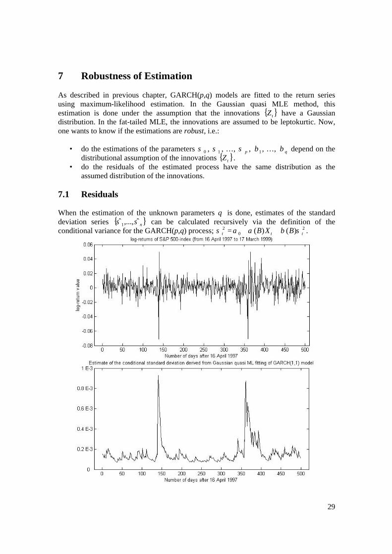
7.1 Residuals When the estimation of the unknown parameters θ is done, estimates of the standard deviation series { }nσσ ˆ,...,ˆ1 can be calculated recursively via the definition of the conditional variance for the GARCH(p,q) process; 2
02 )()( ttt BXB σβαασ ++= .
30
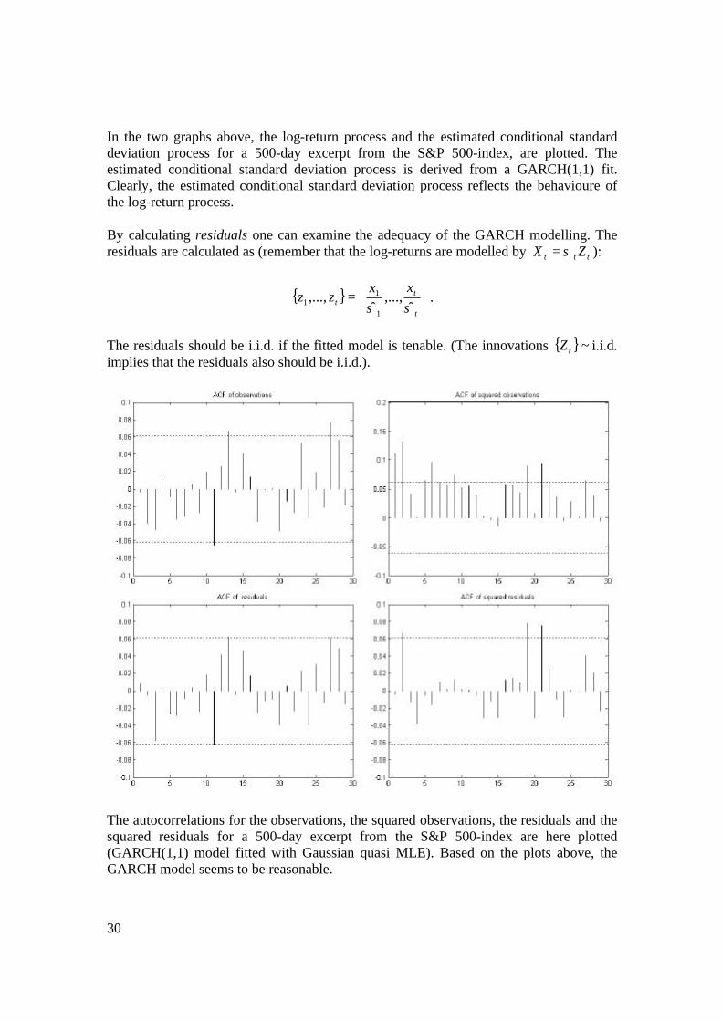
In the two graphs above, the log-return process and the estimated conditional standard deviation process for a 500-day excerpt from the S&P 500-index, are plotted. The estimated conditional standard deviation process is derived from a GARCH(1,1) fit. Clearly, the estimated conditional standard deviation process reflects the behavioure of the log-return process. By calculating residuals one can examine the adequacy of the GARCH modelling. The residuals are calculated as (remember that the log-returns are modelled by ttt ZX σ= ):
{ }
=t
tt
xxzz
σσ ˆ,...,
ˆ,...,
1
11 .
The residuals should be i.i.d. if the fitted model is tenable. (The innovations { }~tZ i.i.d. implies that the residuals also should be i.i.d.).
The autocorrelations for the observations, the squared observations, the residuals and the squared residuals for a 500-day excerpt from the S&P 500-index are here plotted (GARCH(1,1) model fitted with Gaussian quasi MLE). Based on the plots above, the GARCH model seems to be reasonable.
31
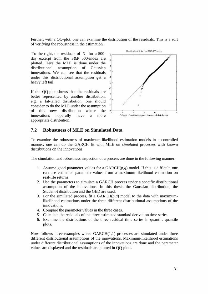
Further, with a QQ-plot, one can examine the distribution of the residuals. This is a sort of verifying the robustness in the estimation. To the right, the residuals of tX for a 500-day excerpt from the S&P 500-index are plotted. Here the MLE is done under the distributional assumption of Gaussian innovations. We can see that the residuals under this distributional assumption get a heavy left tail. If the QQ-plot shows that the residuals are better represented by another distribution, e.g. a fat-tailed distribution, one should consider to do the MLE under the assumption of this new distribution where the innovations hopefully have a more appropriate distribution. 7.2 Robustness of MLE on Simulated Data To examine the robustness of maximum-likelihood estimation models in a controlled manner, one can do the GARCH fit with MLE on simulated processes with known distributions on the innovations. The simulation and robustness inspection of a process are done in the following manner:
1. Assume good parameter values for a GARCH(p,q) model. If this is difficult, one can use estimated parameter-values from a maximum-likelihood estimation on real-life returns.
2. Use the parameters to simulate a GARCH process under a specific distributional assumption of the innovations. In this thesis the Gaussian distribution, the Student-t distribution and the GED are used.
3. For the simulated process, fit a GARCH(p,q) model to the data with maximum-likelihood estimations under the three different distributional assumptions of the innovations.
4. Compare the parameter values in the three cases. 5. Calculate the residuals of the three estimated standard derivation time series. 6. Examine the distributions of the three residual time series in quantile-quantile
plots. Now follows three examples where GARCH(1,1) processes are simulated under three different distributional assumptions of the innovations. Maximum-likelihood estimations under different distributional assumptions of the innovations are done and the parameter values are displayed and the residuals are plotted in QQ-plots.
32
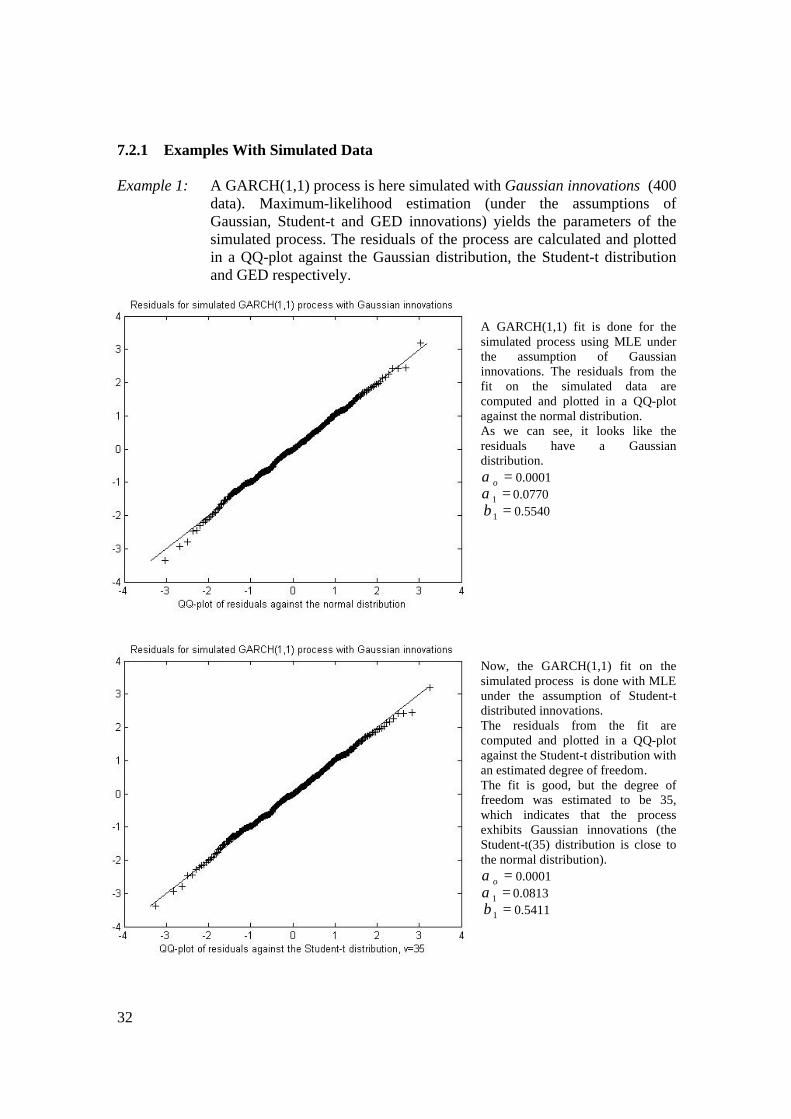
7.2.1 Examples With Simulated Data Example 1: A GARCH(1,1) process is here simulated with Gaussian innovations (400
data). Maximum-likelihood estimation (under the assumptions of Gaussian, Student-t and GED innovations) yields the parameters of the simulated process. The residuals of the process are calculated and plotted in a QQ-plot against the Gaussian distribution, the Student-t distribution and GED respectively.
A GARCH(1,1) fit is done for the simulated process using MLE under the assumption of Gaussian innovations. The residuals from the fit on the simulated data are computed and plotted in a QQ-plot against the normal distribution. As we can see, it looks like the residuals have a Gaussian distribution.
=oα 0.0001 =1α 0.0770 =1β 0.5540
Now, the GARCH(1,1) fit on the simulated process is done with MLE under the assumption of Student-t distributed innovations. The residuals from the fit are computed and plotted in a QQ-plot against the Student-t distribution with an estimated degree of freedom. The fit is good, but the degree of freedom was estimated to be 35, which indicates that the process exhibits Gaussian innovations (the Student-t(35) distribution is close to the normal distribution).
=oα 0.0001 =1α 0.0813 =1β 0.5411
33
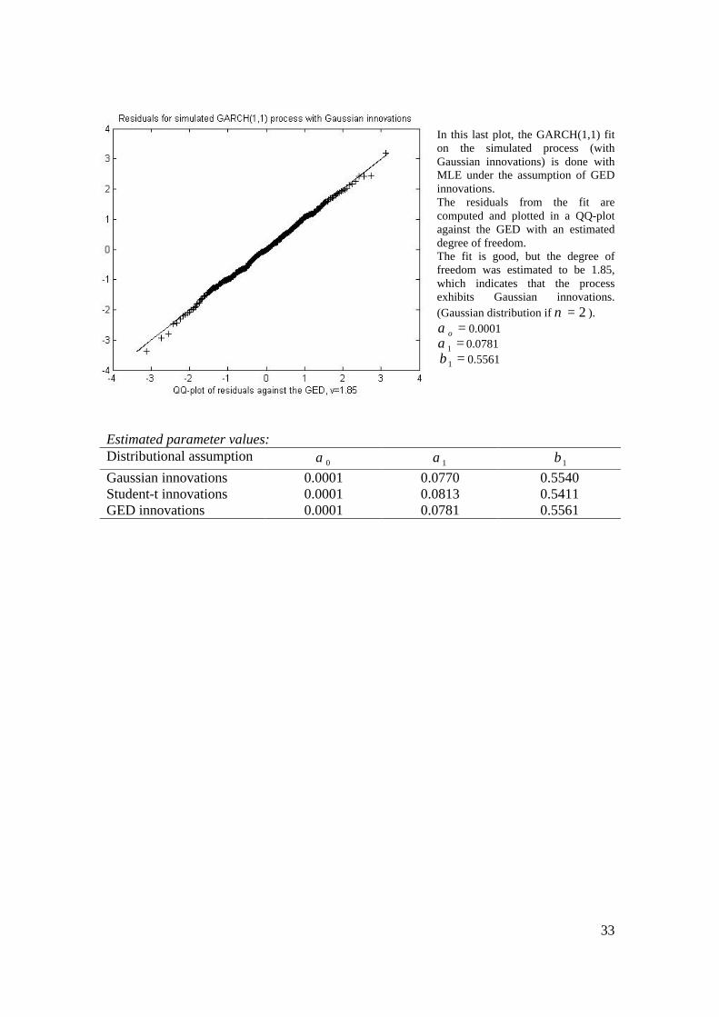
In this last plot, the GARCH(1,1) fit on the simulated process (with Gaussian innovations) is done with MLE under the assumption of GED innovations. The residuals from the fit are computed and plotted in a QQ-plot against the GED with an estimated degree of freedom. The fit is good, but the degree of freedom was estimated to be 1.85, which indicates that the process exhibits Gaussian innovations. (Gaussian distribution if 2=ν ).
=oα 0.0001 =1α 0.0781 =1β 0.5561
Estimated parameter values: Distributional assumption 0α 1α 1β Gaussian innovations 0.0001 0.0770 0.5540 Student-t innovations 0.0001 0.0813 0.5411 GED innovations 0.0001 0.0781 0.5561
34
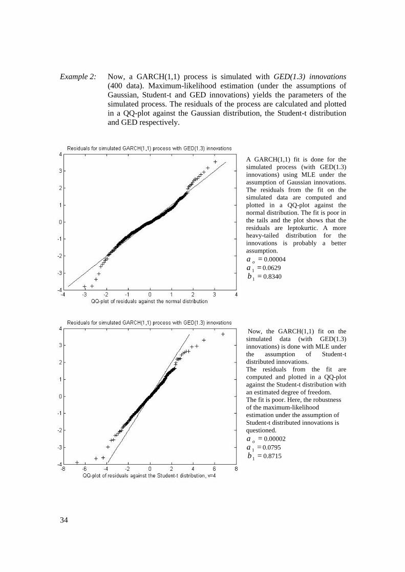
Example 2: Now, a GARCH(1,1) process is simulated with GED(1.3) innovations (400 data). Maximum-likelihood estimation (under the assumptions of Gaussian, Student-t and GED innovations) yields the parameters of the simulated process. The residuals of the process are calculated and plotted in a QQ-plot against the Gaussian distribution, the Student-t distribution and GED respectively.
A GARCH(1,1) fit is done for the simulated process (with GED(1.3) innovations) using MLE under the assumption of Gaussian innovations. The residuals from the fit on the simulated data are computed and plotted in a QQ-plot against the normal distribution. The fit is poor in the tails and the plot shows that the residuals are leptokurtic. A more heavy-tailed distribution for the innovations is probably a better assumption.
=oα 0.00004 =1α 0.0629 =1β 0.8340
Now, the GARCH(1,1) fit on the simulated data (with GED(1.3) innovations) is done with MLE under the assumption of Student-t distributed innovations. The residuals from the fit are computed and plotted in a QQ-plot against the Student-t distribution with an estimated degree of freedom. The fit is poor. Here, the robustness of the maximum-likelihood estimation under the assumption of Student-t distributed innovations is questioned.
=oα 0.00002 =1α 0.0795 =1β 0.8715
35
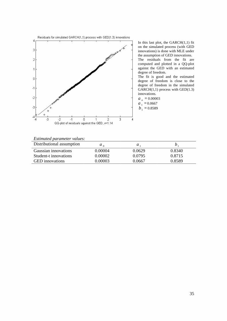
In this last plot, the GARCH(1,1) fit on the simulated process (with GED innovations) is done with MLE under the assumption of GED innovations. The residuals from the fit are computed and plotted in a QQ-plot against the GED with an estimated degree of freedom. The fit is good and the estimated degree of freedom is close to the degree of freedom in the simulated GARCH(1,1) process with GED(1.3) innovations.
=oα 0.00003 =1α 0.0667 =1β 0.8589
Estimated parameter values: Distributional assumption 0α 1α 1β Gaussian innovations 0.00004 0.0629 0.8340 Student-t innovations 0.00002 0.0795 0.8715 GED innovations 0.00003 0.0667 0.8589
36
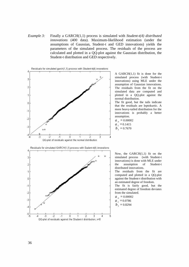
Example 3: Finally a GARCH(1,1) process is simulated with Student-t(4) distributed innovations (400 data). Maximum-likelihood estimation (under the assumptions of Gaussian, Student-t and GED innovations) yields the parameters of the simulated process. The residuals of the process are calculated and plotted in a QQ-plot against the Gaussian distribution, the Student-t distribution and GED respectively.
A GARCH(1,1) fit is done for the simulated process (with Student-t innovations) using MLE under the assumption of Gaussian innovations. The residuals from the fit on the simulated data are computed and plotted in a QQ-plot against the normal distribution. The fit good, but the tails indicate that the residuals are leptokurtic. A more heavy-tailed distribution for the innovations is probably a better assumption.
=oα 0.00002 =1α 0.1415 =1β 0.7670
Now, the GARCH(1,1) fit on the simulated process (with Student-t innovations) is done with MLE under the assumption of Student-t distributed innovations. The residuals from the fit are computed and plotted in a QQ-plot against the Student-t distribution with an estimated degree of freedom. The fit is fairly good, but the estimated degree of freedom deviates from the simulated.
=oα 0.00002 =1α 0.0786 =1β 0.8294
37
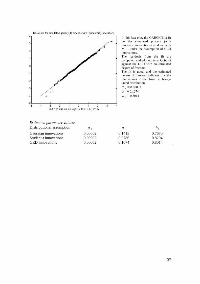
In this last plot, the GARCH(1,1) fit on the simulated process (with Student-t innovations) is done with MLE under the assumption of GED innovations. The residuals from the fit are computed and plotted in a QQ-plot against the GED with an estimated degree of freedom. The fit is good, and the estimated degree of freedom indicates that the innovations come from a heavy-tailed distribution.
=oα 0.00002 =1α 0.1074 =1β 0.8014
Estimated parameter values: Distributional assumption 0α 1α 1β Gaussian innovations 0.00002 0.1415 0.7670 Student-t innovations 0.00002 0.0786 0.8294 GED innovations 0.00002 0.1074 0.8014
38
7.2.2 Conclusion of Examples First, by looking at the estimated parameters for the different distributional assumptions, one can conclude that the models seem to be robust. The values of the estimated parameters do not differ from each other much under the different distributional assumptions. The plots in the examples indicate that the MLE is robust under the assumptions of Gaussian and GED distributed innovations. The overall performance for the MLE under the assumption of Student-t distributed innovations is yet not convincing. The examples support the usefulness of QQ-plots as tools for examining the residuals. With the aid of the QQ-plots, an appropriate model can be chosen. If the innovations come from a Gaussian distribution, the maximum-likelihood estimations are good independent of the assumed distributions. The two MLE models that assume fat-tailed distributions for the innovations assign the degree of freedom so that the fat-tailed distribution is close to the Gaussian. On the other hand, if the innovations come from a fat-tailed distribution, the best fit is achieved with an MLE that assumes GED innovations. The maximum-likelihood estimation under the distributional assumption of Student-t distributed innovations is questioned. The overall performance for the estimation under the assumption of Student-t distributed innovations is not convincing. This robustness examination can be used to choose the right estimation model for given data.
1. Estimate the parameters under the assumption of Gaussian innovations. 2. Plot the residuals in a QQ-plot against the normal distribution. If the residuals are
leptokurtic probably a better distributional assumption is a fat-tailed distribution, e.g. GED innovations.
3. Now, estimate the parameters under the assumption of leptokurtic innovations, e.g. GED.
4. Plot the residuals in a QQ-plot against the chosen leptokurtic distribution. If the fit is good, the distributional assumption most probably is correct.
The simulations in this example consist of only 400 simulated data. Larger simulated sample sizes should give us more information, but large samples imply problems with the stationary assumption of { }tX .
39
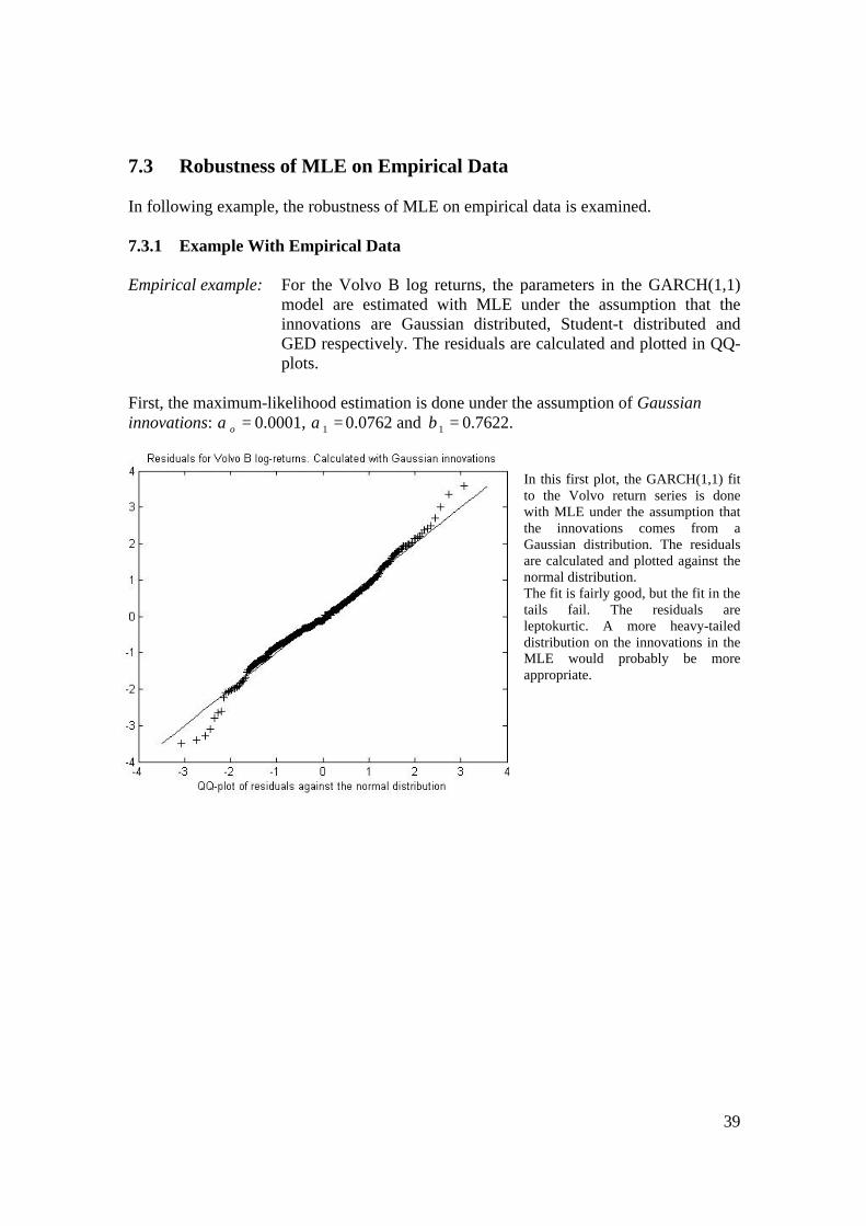
7.3 Robustness of MLE on Empirical Data In following example, the robustness of MLE on empirical data is examined. 7.3.1 Example With Empirical Data Empirical example: For the Volvo B log returns, the parameters in the GARCH(1,1)
model are estimated with MLE under the assumption that the innovations are Gaussian distributed, Student-t distributed and GED respectively. The residuals are calculated and plotted in QQ-plots.
First, the maximum-likelihood estimation is done under the assumption of Gaussian innovations: =oα 0.0001, =1α 0.0762 and =1β 0.7622.
In this first plot, the GARCH(1,1) fit to the Volvo return series is done with MLE under the assumption that the innovations comes from a Gaussian distribution. The residuals are calculated and plotted against the normal distribution. The fit is fairly good, but the fit in the tails fail. The residuals are leptokurtic. A more heavy-tailed distribution on the innovations in the MLE would probably be more appropriate.
40
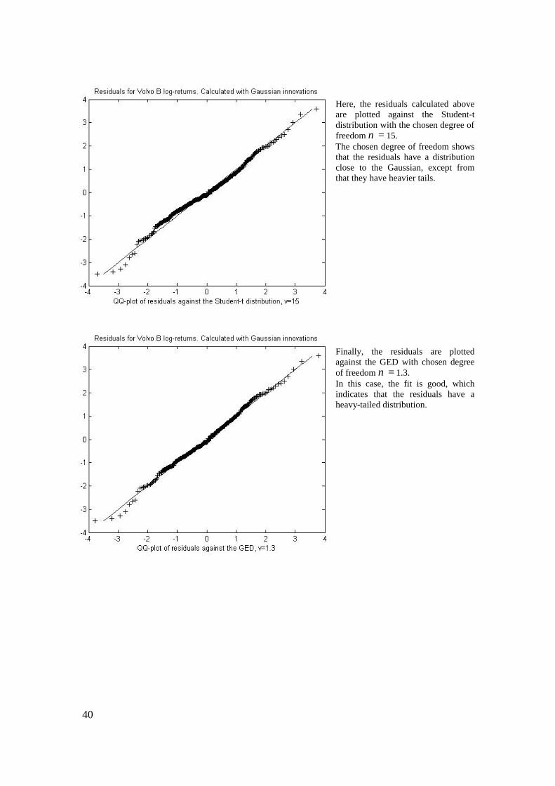
Here, the residuals calculated above are plotted against the Student-t distribution with the chosen degree of freedom =ν 15. The chosen degree of freedom shows that the residuals have a distribution close to the Gaussian, except from that they have heavier tails. Finally, the residuals are plotted against the GED with chosen degree of freedom =ν 1.3. In this case, the fit is good, which indicates that the residuals have a heavy-tailed distribution.
41
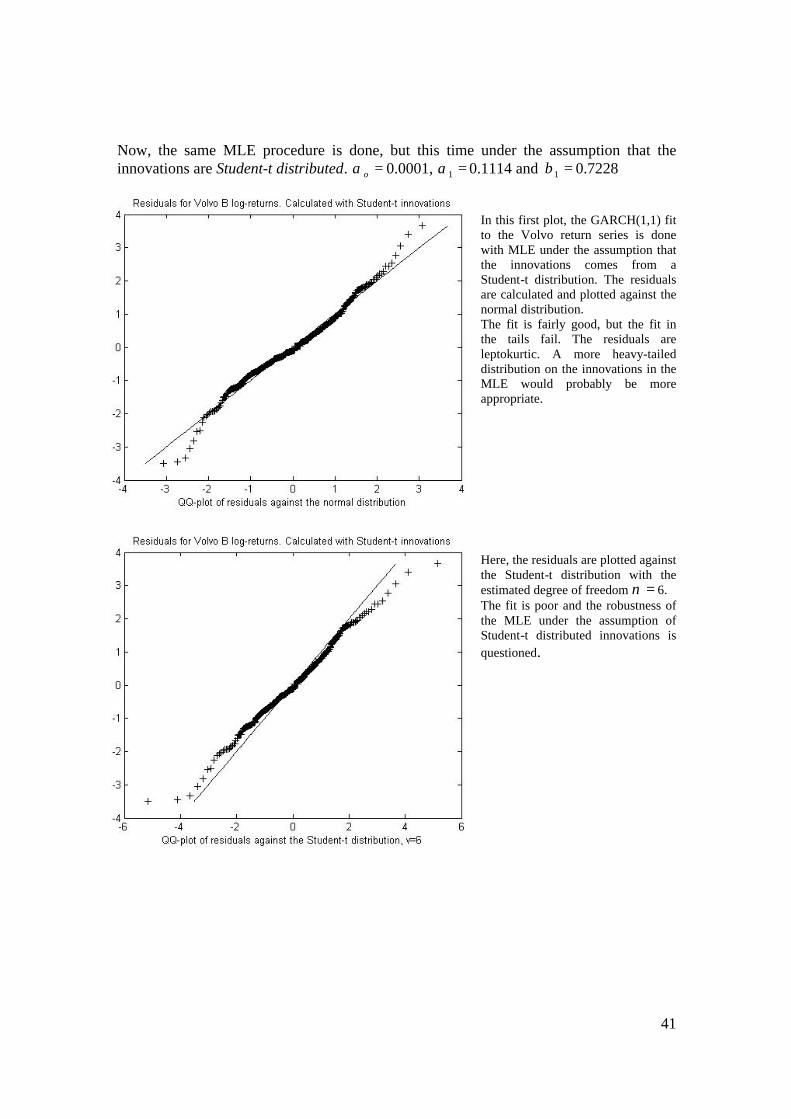
Now, the same MLE procedure is done, but this time under the assumption that the innovations are Student-t distributed. =oα 0.0001, =1α 0.1114 and =1β 0.7228
In this first plot, the GARCH(1,1) fit to the Volvo return series is done with MLE under the assumption that the innovations comes from a Student-t distribution. The residuals are calculated and plotted against the normal distribution. The fit is fairly good, but the fit in the tails fail. The residuals are leptokurtic. A more heavy-tailed distribution on the innovations in the MLE would probably be more appropriate. Here, the residuals are plotted against the Student-t distribution with the estimated degree of freedom =ν 6. The fit is poor and the robustness of the MLE under the assumption of Student-t distributed innovations is questioned.
42
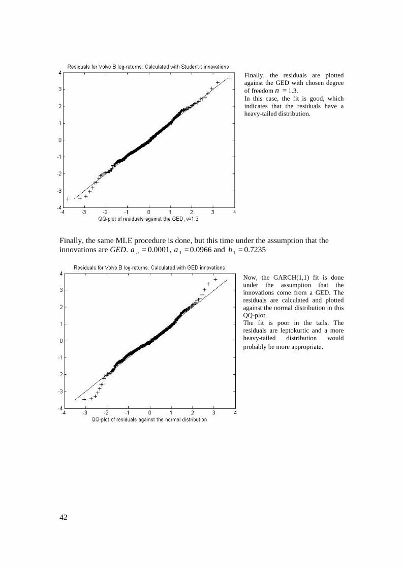
Finally, the residuals are plotted against the GED with chosen degree of freedom =ν 1.3. In this case, the fit is good, which indicates that the residuals have a heavy-tailed distribution.
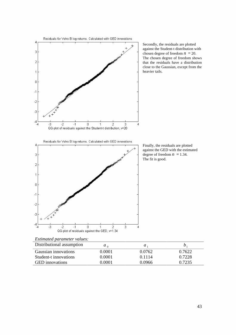
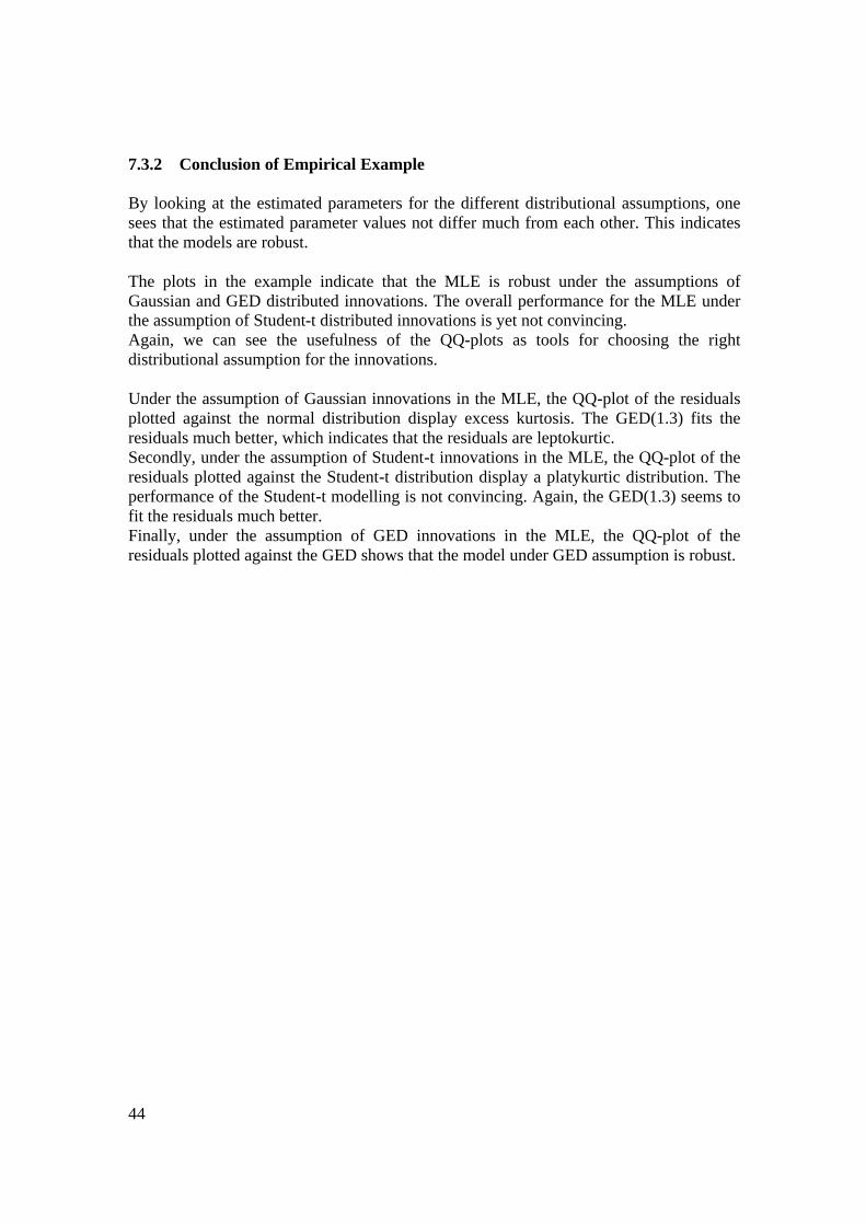
Finally, the same MLE procedure is done, but this time under the assumption that the innovations are GED. =oα 0.0001, =1α 0.0966 and =1β 0.7235
Now, the GARCH(1,1) fit is done under the assumption that the innovations come from a GED. The residuals are calculated and plotted against the normal distribution in this QQ-plot. The fit is poor in the tails. The residuals are leptokurtic and a more heavy-tailed distribution would probably be more appropriate.
43
Secondly, the residuals are plotted against the Student-t distribution with chosen degree of freedom =ν 20. The chosen degree of freedom shows that the residuals have a distribution close to the Gaussian, except from the heavier tails. Finally, the residuals are plotted against the GED with the estimated degree of freedom =ν 1.34. The fit is good.
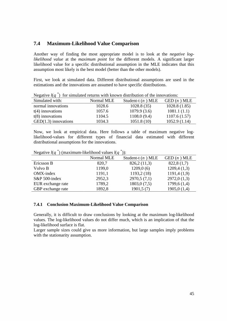
Estimated parameter values: Distributional assumption 0α 1α 1β Gaussian innovations 0.0001 0.0762 0.7622 Student-t innovations 0.0001 0.1114 0.7228 GED innovations 0.0001 0.0966 0.7235
44
7.3.2 Conclusion of Empirical Example By looking at the estimated parameters for the different distributional assumptions, one sees that the estimated parameter values not differ much from each other. This indicates that the models are robust. The plots in the example indicate that the MLE is robust under the assumptions of Gaussian and GED distributed innovations. The overall performance for the MLE under the assumption of Student-t distributed innovations is yet not convincing. Again, we can see the usefulness of the QQ-plots as tools for choosing the right distributional assumption for the innovations. Under the assumption of Gaussian innovations in the MLE, the QQ-plot of the residuals plotted against the normal distribution display excess kurtosis. The GED(1.3) fits the residuals much better, which indicates that the residuals are leptokurtic. Secondly, under the assumption of Student-t innovations in the MLE, the QQ-plot of the residuals plotted against the Student-t distribution display a platykurtic distribution. The performance of the Student-t modelling is not convincing. Again, the GED(1.3) seems to fit the residuals much better. Finally, under the assumption of GED innovations in the MLE, the QQ-plot of the residuals plotted against the GED shows that the model under GED assumption is robust.
45
7.4 Maximum-Likelihood Value Comparison Another way of finding the most appropriate model is to look at the negative log-likelihood value at the maximum point for the different models. A significant larger likelihood value for a specific distributional assumption in the MLE indicates that this assumption most likely is the best model (better than the other models). First, we look at simulated data. Different distributional assumptions are used in the estimations and the innovations are assumed to have specific distributions. Negative l(θ *) for simulated returns with known distribution of the innovations: Simulated with: Normal MLE Student-t (ν ) MLE GED (ν ) MLE normal innovations 1028.6 1028.8 (35) 1028.8 (1.85) t(4) innovations 1057.6 1079.9 (3.6) 1081.1 (1.1) t(8) innovations 1104.5 1108.0 (9.4) 1107.6 (1.57) GED(1.3) innovations 1034.3 1051.8 (10) 1052.9 (1.14) Now, we look at empirical data. Here follows a table of maximum negative log-likelihood-values for different types of financial data estimated with different distributional assumptions for the innovations. Negative l(θ *) (maximum-likelihood values l(θ *)): Normal MLE Student-t (ν ) MLE GED (ν ) MLE Ericsson B 820,7 826,2 (11,3) 822,8 (1,7) Volvo B 1199,0 1209,0 (6) 1209,4 (1,3) OMX-index 1191,1 1193,2 (18) 1191,4 (1,9) S&P 500-index 2952,3 2970,5 (7,1) 2972,0 (1,3) EUR exchange rate 1789,2 1803,0 (7,5) 1799,6 (1,4) GBP exchange rate 1892,8 1901,5 (7) 1905,0 (1,4) 7.4.1 Conclusion Maximum-Likelihood Value Comparison Generally, it is difficult to draw conclusions by looking at the maximum log-likelihood values. The log-likelihood values do not differ much, which is an implication of that the log-likelihood surface is flat. Larger sample sizes could give us more information, but large samples imply problems with the stationarity assumption.
46
8 Variance Forecasting The GARCH-model considered in this thesis assumes that tσ is a function of the past, i.e., 1−tX , 2−tX , … and 1−tσ , 2−tσ , …, and therefore it is in principle known at time t. For this reason, tσ in connection with the distribution of tZ can be used to give a distributional forecast of tX . Assume for example that tZ is i.i.d. N(0,1). Then conditionally on the past values 1−tX , 1−tσ , 2−tX , 2−tσ , …, today’s return tX has an N(0, 2
tσ ) distribution. ( [ ] [ ] [ ] [ ] 0=== ttttt ZEEZEXE σσ ). This allows one to give a distributional forecast of the values tX . For example, there is a 95% chance that tX assumes values in [-1.96 tσ , 1.96 tσ ]. Hence it is an easy matter to determine the conditional VaR (Value at Risk) of the sequence { }tX . 8.1 GARCH(1,1) Once the parameters of the GARCH-models have been estimated one is interested in the variance forecast for the underlying asset. For the GARCH(1,1) model (given that 111 <+ βα ), the expected value of the one-period variance 2
kt+σ at time t is:
[ ] 2)()(1
)(1 21
111
11
111
02 ≥++
+−+−
= +−
−
+ kE tk
k
tktt σβαβα
βαασσ
where 2
12
102
1 ttt X σβαασ ++=+ .
Derivation of this formula:
• 211
2110
22 +++ ++= ttt X σβαασ
• [ ] [ ] [ ]=++= +++ tttttt EXEE σσβσαασσ 211
2110
22
[ ] [ ] { }[ ] [ ] { } [ ] =
===
===⇒==
222
222
)1,0(i.i.d.~ tttt
tttttt
ENZZEE
tindependenZEXEZX
σσ
σσ
( ) [ ] ( ) 21110
21110 ++ ++=++= tttE σβαασσβαα
• [ ] [ ] [ ] ( ) =++=++= ++++2
21102
212
2102
3 ttttttt EXEE σβαασσβσαασσ
( ) ( ) 21
211
11
211
02
1110110 )()(1
)(1++ ++
+−+−
=++++= tt σβαβα
βαασβααβαα
• etc. With increasing value of k the variance forecast will converge to the unconditional variance with the rate 11 βα + :
)(1 11
02
βαα
σ+−
= .
47
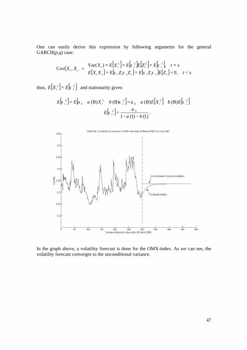
One can easily derive this expression by following arguments for the general GARCH(p,q) case:
( ) [ ] [ ] [ ] [ ][ ] [ ] [ ] [ ]
<=======
=stZEZEZZEXXE
stEZEEXEXXX
ssttssttst
tttttst ,0
,)(Var,Cov
2222
σσσσσσ
thus, [ ] [ ]22tt EXE σ= and stationarity gives:
[ ] [ ] [ ] [ ]220
220
2 B)()B(B)()B( ttttt EXEXEE σβαασβαασ ++=++=
[ ]1)()1(1
02
βαα
σ−−
=⇒ tE .
In the graph above, a volatility forecast is done for the OMX-index. As we can see, the volatility forecast converges to the unconditional variance.
48
8.2 IGARCH For the IGARCH(p,q) models ( 1)1()1( =+ βα ), the conditional expectation of the one period variance 2
kT +σ at time T is:
[ ] 022 ασσ kE TkTT +=+ .
Proof: [ ] [ ] [ ] =++= +++2
112
1102
2 ttt EXEE σβαασ
[ ] [ ] { }[ ] [ ] { } [ ] =
===
===⇒== +
222
2221
)1,0(~ tttt
tttttt
EiidNZZEE
tindependenZEXEZX
σσ
σσ
( ) [ ] 210
21110 ++ +=++= ttE σασβαα
[ ] [ ] [ ] ( ) =++=++= ++++2
21102
212
2102
3 tttt EXEE σβαασβαασ
( ) ( ) 210
21110110 2 ++ +=++++= tt σασβααβαα
etc. ¦ 9 Multivariate GARCH Models Recall chapter 3 where different “stylised facts” about financial data were considered. In addition to these, it is worth mention another “stylised” fact. In financial data the volatilities of different securities very often move together, indicating that there are linkages between markets and that some common factors may explain the temporal variation in conditional second markets. The analysis of many issues in asset pricing and portfolio allocation requires a multivariate framework.
49
10 Appendix A 10.1 Stationarity Definition: { }tX is (weakly) stationary if (i) [ ] oft independen is)( tXEt tX =µ and
(ii) heach for t oft independen is),(),( thtX XXCovtht +=+γ Definition: { }tX is a strictly stationary time series if
( ) ( )´1
´1 ,...,,..., hnh
d
n XXXX ++=
for all integers h and n ≥ 1. (Here d
= is used to indicate that the two random vectors have the same joint distribution function.)
10.2 Proof of Corollary: Strict stationarity implies weak stationarity. (See Theorem in chapter 6.1.1).
• [ ] [ ] { tttt ZEXE σσ == and tZ are independent for every } [ ] [ ] 0== tt ZEEt σ
• ( ) [ ] [ ] [ ] [ ][ ] [ ] [ ] [ ]
<=======
=stZEZEZZEXXE
stEZEEXEXXX
ssttssttst
tttttst when0
when)(Var,Cov
2222
σσσσσσ
thus, [ ] [ ]22tt EXE σ= plus stationarity yields:
[ ] [ ] [ ] [ ]
[ ]1
110
02
220
220
2
11)()1(1
)(
B)()B()()(−
==
+−=
−−==⇒
++=++=
∑∑q
jj
p
iitt
ttttt
EXVar
EXEBXBEE
βααβα
ασ
σβαασβαασ
¦
50
11 References [1] Bollerslev, T. (1986) Generalized Autoregressive Conditional Heteroskedasticity Journal of Econometrics 31, pp. 307-327. [2] Bollerslev, T., Chou, R.Y. and K.F. Kroner (1992) ARCH Modelling in Finance: A Review of the Theory and Empirical Evidence Journal of Econometrics 52, pp. 5-59. [3] Bollerslev, T., Engle R.F. and D.B. Nelson (1994) ARCH Models Handbook of Econometrics vol. 4, pp. 2959-3038. [4] Brockwell, P.J. and R.A. Davis (1991) Time Series: Theory and Methods Springer, New York [5] Brockwell, P.J. and R.A. Davis (1996) Introduction to Time Series and Forecasting Springer, New York [6] Engle, R.F. (1982)
Autoregressive Conditional Heteroskedasticity with Estimates of the Variance of United Kingdom Inflation
Econometrica vol. 50, pp. 987-1007. [7] Engle, R.F. (1995) ARCH Selected Readings Oxford University Press [8] Grandell, J. (1998) Time Series Analysis Lecture notes, KTH Stockholm [9] Hansson, B. and P. Hördahl (1998) Forecasting Variance Using Stochastic Volatility and GARCH
Working Paper Series, Department of Economics, School of Economics and Management, University of Lund
[10] Mikosch, T. (2000) Modelling Dependence and Tails of Financial Time Series http://www.math.ku.dk/~Mikosch/Semstat

51
[11] Palm, F.C. (1996) GARCH Models of Volatility in Maddala, G.S. and C.R. Rao (eds.), Handbook of Statistics, Vol. 14 Amsterdam, Elsevier Science B.V., pp. 209-240. _______ [12] Luenberger, D.G. (1984) Linear and Non-linear Programming (Second Edition) Addison-Wesley, Reading, Massachusetts [13] Standard & Poor The S&P 500 Index (time series) http://www.standardandpoors.com