gary e. - dtic.mil · this report was prepared by gary e. phetteplace, mechanical engineer, martin...

* AD-A247 460

* Field Measurements of Heat LossesFrom Three Types of HeatDistribution SystemsGary E. Phetteplace, Marlin J. Kryska, and David L. Carbee November 1991

DTICELECTE

*MAR 0 19921

a 0]

f l e~ ,br QPPiovedio, ubik,. rejoase and sale; i= tdl strbution is unjimite4L

a!

For conversion of SI metric units to U.S./British customary unitsof measurement consult ASTM Standard E380, Metric PracticeGuide, published by the American Society for Testing andMaterials, 1916 Race St., Philadelphia, Pa. 19103.

This report is printed on paper that contains a minimum of50% recycled material.

Special Report 91-19

U.S. Army Corpsof EngineersCold Regions Research &Engineering Laboratory

Field Measurements of Heat LossesFrom Three Types of HeatDistribution SystemsGary E. Phetteplace, Martin J. Kryska, and David L. Carbee November 1991

,TEO

Ux:....:j

S;,, _

ByDi' .!h tio, I1

-F .:..,:,i . : ......... .

Dist ..i;-

92-057291111 1 IIII III I ltl i 111Prepared forU.S. ARMY ENGINEERING AND HOUSING SUPPORT CENTER

Approved for public releose; distribution is unlimited.

92 3 039 219

PREFACE

This report was prepared by Gary E. Phetteplace, Mechanical Engineer, Martin J. Kryska,Mechanical Engineer, and David L. Carbee, Engineering Technician, Applied ResearchBranch, Experimental Engineering Division, U.S. Army Cold Regions Research and EngineeringLaboratory.

Funding forthis research was provided by the U.S. Army Facilities Engineering ApplicationsProgram, Work Unit 10/015.

The authors acknowledge the careful technical reviews of this report given by the followingindividuals: F. Donald Haynes, Dr. Virgil Lunardini, and Herbert Ueda of CRREL and VernonMeyer of the Missouri River Division. The many useful comments they each provided helpedto improve the content and clarity of this report. The authors would also like to acknowledgeseveral individuals who contributed to this study in various ways: Nancy Greely, Gary Trachier,Robert Bigl, and Richard Roberts of CRREL; and Frank Hall of the U.S. Army Corps ofEngineers, Ft. Jackson Area Office, and Michael Munn of the Ft. Jackson Directorate ofEngineering and Housing.

The contents of this report are not to be used for advertising or promotional purposes. Citationof brand names does not constitute an official endorsement or approval of the use of suchcommercial products.

CONTENTS

Preface ............................................................................................................................................ iiIntroduction ..................................................................................................................................... 1

Problem statem ent ...................................................................................................................... IObjective and approach .............................................................................................................. 1

System description and instrum entation layout ............................................................................. ICom m on conduit system ............................................................................................................ IIndividual conduit system ......................................................................................................... . 3Shallow concrete trench system ................................................................................................ . 3Therm al insulation ..................................................................................................................... 5Instrum entation layout ............................................................................................................... 5G eneral description of instrum entation ...................................................................................... 5Data logging and com m unication system s ................................................................................ 8Data acquisition schedule and coverage .................................................................................... 10Soil classification and m oisture content data ............................................................................. 10

M ethods of data analysis ................................................................................................................ I ID ata processing .......................................................................................................................... 11Description of calculation m ethods ........................................................................................... 11

Results ............................................................................................................................................. 16Trench site .................................................................................................................................. 16Com m on conduit site ................................................................................................................. 22Individual conduit site ................................................................................................................ 24

Conclusions ..................................................................................................................................... 27Literature cited ................................................................................................................................ 27A ppendix A : Sensor locations ........................................................................................................ 29A bstract ........................................................................................................................................... 35

ILLUSTRATIONS

Figure1. Com m on conduit site details ............................................................................................... 22. Individual conduit site details ............................................................................................. 33. Trench site construction details .......................................................................................... 64. Data as recorded by data logging system 1, trench and common conduit sites ................... 95. Data as recorded by data logging system 2, individual conduit site .................................... 106. Trench air tem perature over the study period ...................................................................... 187. Trench tem peratures for 1986-1987 .................................................................................... 188. Trench tem peratures for 1988-1989 .................................................................................... 199. Heat losses for the trench site over the study period ........................................................... 20

10. Heat flux sensor data for the trench site ............................................................................... 2011. Com m on conduit site tem peratures ..................................................................................... 2212. Com m on conduit site heat loss for 1986-1987 .................................................................... 2313. Com m on conduit heat loss for 1988-1989 .......................................................................... 2314. Individual conduit site tem peratures ................................................................................... 2615. Average undisturbed soil temperature at 74 in. and fitted sinusoidal curve ........................ 2616. Individual conduit site heat losses ...................................................................................... 2617. Heat flux sensor data for the individual conduit site, 10 day averages ................................ 27

TABLES

Table1. Therm al properties of m ineral wool pipe insulation ........................................................... 82. Data scan frequencies for each site ...................................................................................... I I3. Tim e periods for which data were collected ........................................................................ 124. Soil data from com m on conduit site .................................................................................... 135. Soil data from individual conduit site .................................................................................. 136. Selected raw and reduced data for the trench site ................................................................ 177. Selected raw and reduced data from the common conduit site ............................................ 218. Selected raw and reduced data from the individual conduit site .......................................... 25

iii

Field Measurements of Heat Losses FromThree Types of Heat Distribution Systems

GARY E. PHETIEPLACE, MARTIN J. KRYSKA, AND DAVID L. CARBEE

INTRODUCTION the quantification of heat losses from operating heatdistribution piping systems. This project is ajoint effort

Problem statement between two of the U.S. Army Corps of EngineersMost major Department of Defense facilities are Laboratories: CRREL and the Construction Engineer-

heated with central heat distribution systems. The heat ing Research Laboratory (CERL). This report describesfrom the central heating plants is usually distributed to only the portion of the work for which CRREL wasthe buildings as high temperature hot water or steam responsible. Ajoint report on the project will be availablethrough buried piping systems. DoD has approximately at a later date.6,000 miles of heat distribution piping systems in ser- From the discussion presented above it is clear thatvice (Segan and Chen 1984). The Army owns and heat losses are a major portion of the operations andoperates over 3,000 miles of this (Department of the maintenance (O&M) costs for heat distribution systems.Army 1988). Many of our systems are old and in need In spite of this, little emphasis has been placed on theof major repairs or replacement. To replace these sys- thermal design of these systems and the subsequenttems currently costs about $300 per lineal foot. Thus we operational costs. To date heat losses have been calcu-are facing monumental costs for replacement. In addi- lated based on formulas that rely on several untestedtion, the technology now being used by DoD is prob- assumptions. The work described here represents one oflematic, and many systems that have been recently the first efforts to measure actual heat losses fromreplaced have failed prematurely. A previous study by operational systems and compare these measurementsthe Corps of Engineers (Segan and Chen 1984) identi- with calculated results. Other efforts are currently un-fied many problems caused by improper design, in- derway to make similar types of measurements on otherstallation and maintenance. Most of these problems led types of systems (Phetteplace 1990) and under closelyto premature failure of the system. controlled laboratory conditions (Lunardini 1990).

Capital costs and system life are only a portion of the To accomplish our objective we chose to instrumentlife-cycle cost issue. These systems are very costly to an operating system on an Army facility. Ft. Jackson,operate and maintain as well. If we assume an optimistic South Carolina, which was selected because a largevalue for system losses of 50 Btu/hr-ft (foraged systems replacement project was underway there. Three types ofa value of several times this is likely) and a cost of $10 buried heat distribution piping systems were installed:per million Btu for heat energy, we find that heat losses I. Shallow concrete trench with top cover at gradecost the Army around $85 million per year. The FY 88 level."Redbook" (U.S. Army 1988) gives annual mainte- 2. Class A steel conduit system with supply andnance costs of over $41 million. This, of course, does return piping in a common conduit.not include any significant replacement projects. 3. Class A steel conduit system with supply and

return piping in individual conduits.Objective and approach

The objective of DoD heat distribution research is toidentify improvements in methods and systems that will SYSTEM DESCRIPTION ANDprove to be less costly and problematic. This report INSTRUMENTATION LAYOUTdescribes a portion of the work underway in a FacilitiesEngineering Applications Program (FEAP) project that Common conduit systemhas this objective. This project is funded by the Army's The prefabricated common conduit system, both theEngineering and Housing Support Center (EHSC). The supply and return piping in the same steel conduit (Fig.portion of the project covered by this report deals with I), conforms to the federal agency criteria for a Class A

Thermocouple StringsC C2

Building "2-

2255

Buried

Instrument Cable

400

$R

Concrete Thermocouple 24.7'Pad String C2 22.8'

1222

Sidewalk

CommonConduit

10

a. Instrumentation site with thermocouple c. Ground thermocouple locations.strings and cable locations.

Ir aInstrumentationb

Sealed Cable 4-in.Access PlugC reu 2Thermocouple

121 138in.

SUPPLY MThc Insulation

S l5-in. Supy and

RETURN Heat Flux • Return PipeSensors

b. Isometric view of instrumented pipe and conduit d. Pipe thermocouple and sensor location.

Figure 1. Common conduit site details.

Intrmetaio 42n

system. This type of system is designed and installed in signed to be drainable and dryable. The integrity of theaccordance with Corps of Engineers Guide Specifica- air space can be checked by pressure testing at 15 psig.tion (CEGS) 02695 (U.S. Army 1989).

The Class A conduit system used at Ft. Jackson Individual conduit systemconsists of schedule 40 steel supply and return pipes of The individual conduit system employs the same5-in. nominal pipe size (NPS). These pipes are insulated construction features as the common conduit systemwith a mineral wool insulation of 1.5-in. thickness. The described above. In this case the supply and return pipesinsulated supply and return pipes are encased in a spiral- are of 4-in. NPS Schedule 40 steel and each is encasedwound steel conduit that is approximately 1/8 in. thick. in its own individual conduit of approximately 16-in.The supply and return pipes are oriented vertically outer diameter (Fig. 2). The insulation on the pipes iswithin the conduit with the supply pipe on top of the 2.5-in.-thick mineral wool in each case.return pipe. The conduit has an outer diameter of ap-proximately 20 in., thus allowing for an air space Shallow concrete trench systembetween the pipe insulation and inside of the conduit. The shallow concrete trench system consists of aThe conduit is covered with an asphalt-based corrosion- cast-in-place concrete trench with cast-in-place con-resistant coating. All field closures of the conduit are crete covers (Fig. 3). The system is designed such thatwelded and coated. The interior air space between the the top surface of the covers is slightly above thepipe insulation and the conduit inner diameter is de- surrounding grade level and can be used as a sidewalk.

Building 3276 Building 3285

13' 13

IndividualConduits

IThermocouple

Strings Existing- 8" CHW

Existing4" HTW

40'

-30'

Manhole

(w/instrumentation access)

a. Instrumentation site with thermocouple string locations.

Figure 2. Individual conduit site details.

3

Sealed InstrumentationAccess Plugs Cables

Thermocouples

Heat Flux

Sensors

b. Isometric view of instrumented pipe and conduit.

Figure 2. (cont'd).

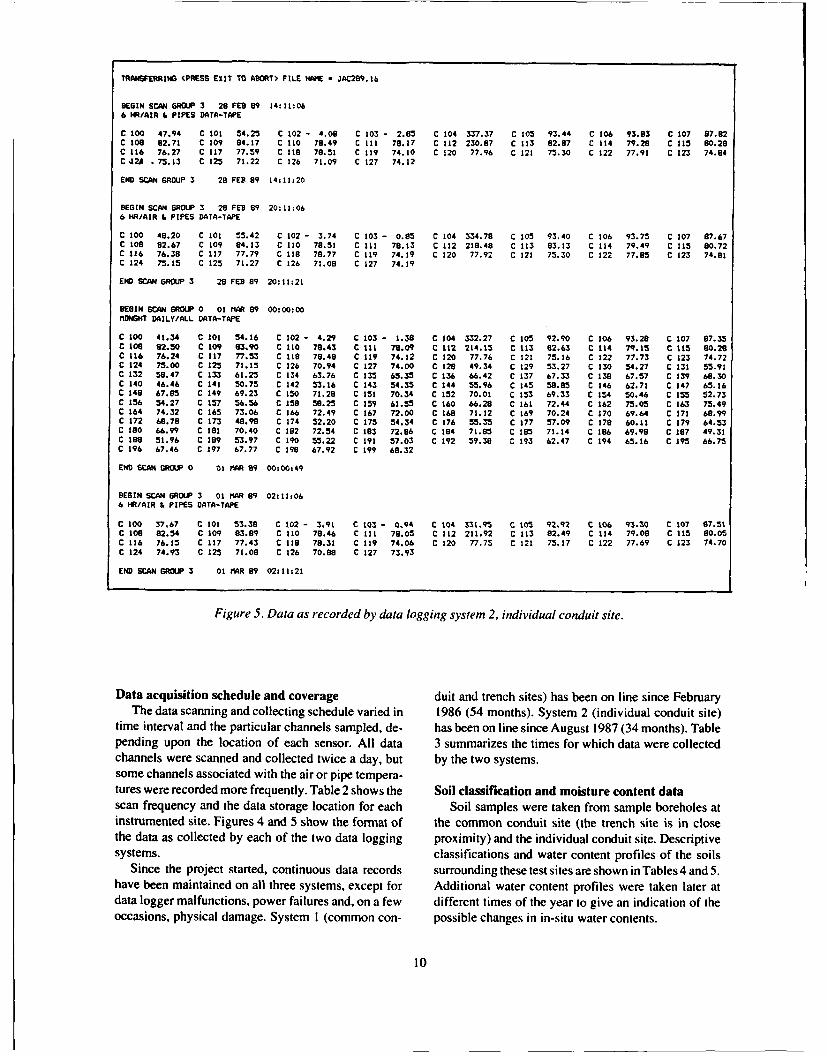
The covers have lifting eyes cast into them and thus they cided to use an average of the two for this study. Thecan be removed in the event that the system must be average value is within 10% of each of the two insula-serviced. The pipes are supported by pillars protruding tion thermal conductivities in every case. The thermalfrom the floor. This allows any water that enters the properties of each insulation and the average value usedtrench to drain to the manholes where it can be removed are given in Table 1. For the calculations an equationby sump pumps or gravity drainage, was fitted to the average insulation thermal conductiv-

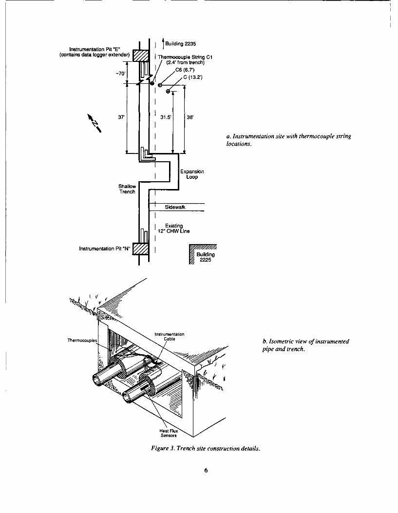
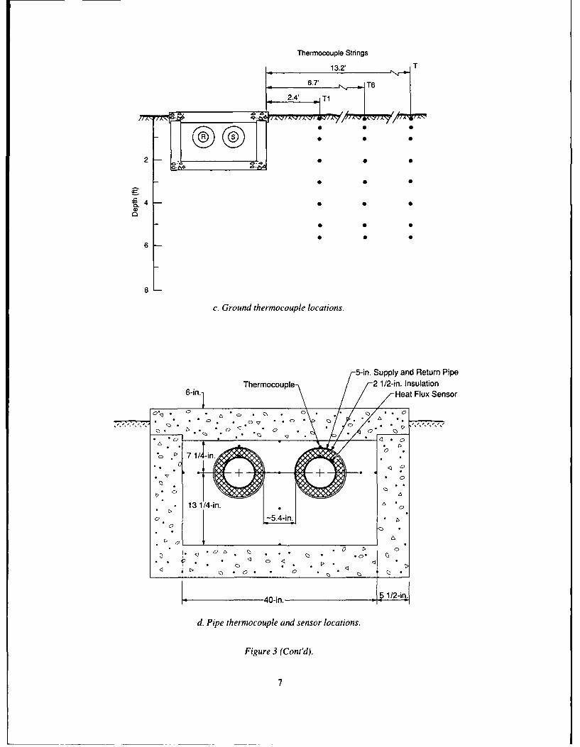
The interior dimensions of the shallow concrete ity data:trench at the Ft. Jackson test site are 40 in.wide and 21.5in. high. The trench walls are 5.5 in. thick. The thickness k. = 0.0233 - (4.17 x 10- 3T) + (8.33 x I OT?)of the trench covers can be varied as required for theloading expected. At our Ft. Jackson test site the trenchcovers are 6 in. thick and have a lip of about I in. at the where ki is average thermal conductivity and Ti is meanoutside edge, so that the portion resting on the trench insulation temperature (°F).wall is about 5 in. thick. The supply and return piping is5-in. NPS schedule 40 steel. Each pipe is insulated with Instrumentation layout2.5 in. of mineral wool pipe insulation. The location of the temperature and heat flux sensors

as well as the approximate location of the sites them-Thermal insulation selves are shown in Figures 1,2, and 3 for the common

Only two manufacturers of mineral wool insulation conduit, trench and individual conduit sites, respec-have a product approved for use on underground heat tively.distribution systems. We were not able to determinewhich product had been used on each of the systems in General description of instrumentationthis study. Since the thermal properties of the two Heat flow measurements were taken at each siteapproved insulations are somewhat different, we de- using commercially available heat flux transducers

4

Thermocouple Stringsz Y X W V

2

a 10

166

70in

Hea Flu Seso

12 1 Ad-i). 6 in 0 d

. Gron thermocouple dsn locations.

Figure 1 1/4-int'd. 16diin.a conduitsiedtl.

5

Instrumentation Pit "E" ijBilding 2235

(contains data logger extender) Thermocouple String C1(2.4' from trench)

7C6 (6.7')7,C (13.2')

37' 31.5 36'

a. Instrumentation site with thermocouple string

locations.

ExpansionLoop

ShallowTrench

Sidewalk

Existing12" CHW Line

Instrumentation Pit "N" 7 uBlding

i2225

Instrumentation

rhermocouples Ce b. Isometric view of instrumented

pipe and trench.

Figure 3. Trench site construction details.

6

Thermocouple Strings

00

* 0 0

6

8L

c. Ground thermocouple locations.

5-in. Supply and Return PipeThermocouple r 2 1/2-in. Insulation

6-in. H eat Flux Sensor0 0

, . .o . . .0 . . .

0

00

0 0C 0

> <A

40-in 5 "12-i0

d. Pip throcul an esrlctos

Figure__________ 3o ACnt

.7A

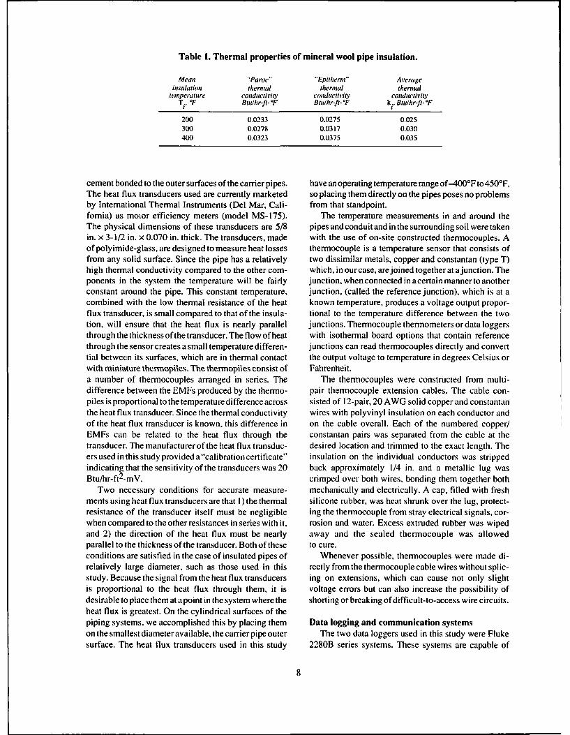
Table 1. Thermal properties of mineral wool pipe insulation.

Mean "Paroc" Epithern" Averageinsulation thermal thermal thermal

temperature conductivity conductivity conductivityT.. F Btu/hr-ft- OF Btu/hr-ft- kF I .. Btu/hr-ft- °F

200 0.0233 0.0275 0.025300 0.0278 0.0317 0.030400 0.0323 0.0375 0.035

cement bonded to the outer surfaces of the carrier pipes. have an operating temperature range of-400*F to4500 F,The heat flux transducers used are currently marketed so placing them directly on the pipes poses no problemsby International Thermal Instruments (Del Mar, Cali- from that standpoint.fornia) as motor efficiency meters (model MS-175). The temperature measurements in and around theThe physical dimensions of these transducers are 5/8 pipes and conduit and in the surrounding soil were takenin. x 3-1/2 in. x 0.070 in. thick. The transducers, made with the use of on-site constructed thermocouples. Aof polyimide-glass, are designed to measure heat losses thermocouple is a temperature sensor that consists offrom any solid surface. Since the pipe has a relatively two dissimilar metals, copper and constantan (type T)high thermal conductivity compared to the other com- which, in our case, are joined together at a junction. Theponents in the system the temperature will be fairly junction, when connected in acertain mannerto anotherconstant around the pipe. This constant temperature, junction, (called the reference junction), which is at acombined with the low thermal resistance of the heat known temperature, produces a voltage output propor-flux transducer, is small compared to that of the insula- tional to the temperature difference between the twotion, will ensure that the heat flux is nearly parallel junctions. Thermocouple thermometers or data loggersthroughthethicknessofthetransducer.Theflowofheat with isothermal board options that contain referencethrough the sensor creates a small temperature differen- junctions can read thermocouples directly and converttial between its surfaces, which are in thermal contact the output voltage to temperature in degrees Celsius orwith miniature thermopiles. The thermopiles consist of Fahrenheit.a number of thermocouples arranged in series. The The thermocouples were constructed from multi-difference between the EMFs produced by the thermo- pair thermocouple extension cables. The cable con-piles is proportional to the temperature difference across sisted of 12-pair, 20 AWG solid copper and constantanthe heat flux transducer. Since the thermal conductivity wires with polyvinyl insulation on each conductor andof the heat flux transducer is known, this difference in on the cable overall. Each of the numbered copper/EMFs can be related to the heat flux through the constantan pairs was separated from the cable at thetransducer. The manufacturer of the heat flux transduc- desired location and trimmed to the exact length. Theers used in this study provided a "calibration certificate" insulation on the individual conductors was strippedindicating that the sensitivity of the transducers was 20 back approximately 1/4 in. and a metallic lug wasBtu/hr-ft2-mV. crimped over both wires, bonding them together both

Two necessary conditions for accurate measure- mechanically and electrically. A cap, filled with freshments using heat flux transducers are that i) the thermal silicone rubber, was heat shrunk over the lug, protect-resistance of the transducer itself must be negligible ing the thermocouple from stray electrical signals, cor-when compared to the other resistances in series with it, rosion and water. Excess extruded rubber was wipedand 2) the direction of the heat flux must be nearly away and the sealed thermocouple was allowedparallel to the thickness of the transducer. Both of these to cure.conditions are satisfied in the case of insulated pipes of Whenever possible, thermocouples were made di-relatively large diameter, such as those used in this rectly from the thermocouple cable wires without splic-study. Because the signal from the heat flux transducers ing on extensions, which can cause not only slightis proportional to the heat flux through them, it is voltage errors but can also increase the possibility ofdesirable to place them at a point in the system where the shorting or breaking of difficult-to-access wire circuits.heat flux is greatest. On the cylindrical surfaces of thepiping systems, we accomplished this by placing them Data logging and communication systemson the smallest diameter available, the carrier pipe outer The two data loggers used in this study were Flukesurface. The heat flux transducers used in this study 2280B series systems. These systems are capable of

8

TRANSFERRING <PRESS EXIT TO ABORT> FILE NAIE = JACK88.16

BEGIN SCAN GROUP 3 20 JUL 88 20:23:07PIPE TEIMPS/TAPE/6N

C 1 330.16 C 2 293.34 C 3 176.10 C 4 157.01 C 5 162.43 C 6 143.56 C 7 177.55 C B 145.72C lB - 8.18 C 19 4.36 C 100 134.20 C 101 110.31 C 102 332.90 C 103 140.95 C 104 132.86 C 105 261.67C 106 146.51 C 107 127.20 C 108 102.98 C 109 109.69 C 110 128.49 C I1 128.64 C 136 1.80 C 137 - 2.94

END SCAN GROUP 3 20 JUL 88 20:23:21

BEGIN SCAN GROUP 1 20 JUL 88 22:23:018IHOU0I Y AIR TEMPS-TAPE

C 0 80.98 C 32 84.70 C 139 86.41 C 100 130.94 C 104 128.32 C 110 124.55 C 111 124.64


BE6IN SCAN GROUP 0 21 JUL 88 00:00:00DAILY/EVERYTHING-TAPE

C 0 78.43 C 1 330.56 C 2 303.88 C 3 176.13 C 4 157.53 C 5 161.77 C 6 143.90 C 7 178.24C 8 145.45 C 9 89.26 C 10 93.00 C It 96.26 C 12 99.48 C 13 103.53 C 14 115.77 C 15 125.66C 16 125.48 C 17 128.49 C 18 - 8.06 C 19 4.17 C 20 92.67 C 21 95.10 C 22 98.04 C 23 101.23C 24 104.33 C 25 109.56 C 26 109.19 C 27 103.40 C 28 98.15 C 29 93.36 C 30 89.40 C 31 89.53C 32 84.47 C 100 130.31 C 101 109.48 C 102 331.19 C 103 136.82 C 104 128.10 C 105 300.25 C 106 141.32C 107 119.56 C 10 103.12 C 109 108.34 C 110 124.87 C 111 124.85 C 112 85.93 C 113 85.68 C 114 83.61C 115 82.21 C 116 82.90 C 117 81.47 C 118 81.67 C 119 82.44 C 120 88.12 C 121 89.24 C 122 88.20C 123 83.28 C 124 79.62 C 125 77.10 C 126 75.63 C 127 75.27 C 128 86.06 C 129 87.05 C 130 84.75C 131 77.81 C 132 68.89 C 133 68.27 C 134 71.05 C 135 71.85 C 136 4.13 C 137 - 2.89 C 139 84.98


BEGIN SCAN GROUP 1 21 JUL 88 00:23:018IHOURLY AIR TEI'PS-TAPE

C 0 78.02 C 32 84.48 C 139 84.51 C 100 130.11 C 104 127.75 C 110 124.19 C 111 124.38


BEGIN SCAN GROUP 1 21 JUL 88 02:23:01SIHOURLY AIR TEIPS-TAPE

C 0 73.58 C 32 84.32 C 139 82.99 C 100 127.76 C 104 125.27 C 110 122.28 C 111 122.36


BEGIN SCAN GROUP 3 21 JUL 88 02:23:07PIPE TEMPS/TAPE/6HR

C I 331.30 C 2 301.89 C 3 176.64 C 4 157.97 C 5 162.42 C 6 144.39 C 7 178.77 C 8 146.14C is - 8.30 C 19 5.13 C 100 127.76 C 101 108.39 C 102 332.87 C 103 133.93 C 104 125.28 C 105 299.65C 106 138.66 C 107 115.80 C 108 102.98 C 109 107.13 C 110 122.34 C III 122.37 C 136 4.18 C 137 - 3.02


Figure 4. Data as recorded by data logging system 1, trench and common conduit sites.

monitoring and logging up to 100 separate inputs, with puter at CRREL by telephone using RS-232 interfacesexpansion to 1,500 inputs using additional remote 100- in the data loggers and modems. This allowed us to notchannel input extenders. The individual input channels only collect and process the data but to keep a closewere monitored and values collected in different scan evaluation of the operation of the utility systems. Thisgroups at different time intervals to accommodate the was done approximately every week.needs of the study. All data scans were stored on a DC One data logger was used to collect values from both100 magnetic tape drive that recorded date, time, scan the trench and common conduit sites and the other wasgroup, channel number and value. Limited data were used for the individual conduit site. Appendix A con-also printed onto paper for backup purposes in the event tains listings of monitored inputs from the three instru-of a problem with the magnetic tape. This also served as mented sites. These tables give the channel number,a quick visual check on the individual channel functions label, output unit and the sensor location. Figures 4 andwhenever we visited the test site. The data collected on 5 are samples of some typical data as collected from themagnetic tape were transferred to our personal com- data logging systems.

9

TRANSFERRING <PRESS EXIT TO ABORT> FILE NAME - JAC289.16

BEGIN SCAN GROIUP 3 28 FEB 89 14:11:066 R/AIR & PIPES DATA-TAPE

C 100 47.94 C 101 54.25 C 102- 4.08 C 103- 2.85 C 104 337.37 C 105 93.44 C 106 93.83 C 107 87.82C 108 82.71 C 109 84.17 C 110 78.49 C 111 79.17 C 112 230.87 C 113 82.87 C 114 79.28 C 215 80.28C 116 76.27 C 117 77.59 C 118 78.51 C 119 74.10 C 120 77.96 C 121 75.30 C 122 77.91 C 123 74.84C.12A . 75.13 C 125 71.22 C 126 71.09 C 127 74.12

END SCAN GROUP 3 28 FEB 89 14:11:20

BEGIN SCAN GROUP 3 28 FEB 89 20:11:066 HR/AIR & PIPES DATA-TAPE

C 100 48.20 C 101 55.42 C 102- 3.74 C 103- 0.85 C 104 334.78 C 105 93.40 C 106 93.75 C 107 87.67C 108 82.67 C 109 84.13 C 110 78.51 C 111 78.13 C 112 218.48 C 113 83.13 C 114 79.49 C 115 80.72C 116 76.38 C 117 77.79 C 118 78.77 C 119 74.19 C 120 77.92 C 121 75.30 C 122 77.85 C 123 74.81C 124 75.15 C 125 71.27 C 126 71.08 C 127 74.19

END SCAN GROUP 3 29 FEB 89 20:11:21

BEGIN SCAN GROUP 0 01 MAR 89 00:00:00MDNGHT DAILY/ALL DATA-TAPE

C 100 41.34 C 101 54.16 C 102 - 4.29 C 103 - 1.38 C 104 332.27 C 105 92.90 C 106 93.28 C 107 87.35C 108 82.50 C 109 63.90 C 110 78.43 C 111 78.09 C 112 24.15 C 113 82.63 C 114 79.15 C 115 60.26C 116 76.24 C 117 77.53 C 118 78.48 C 119 74.12 C 120 77.76 C 121 75.16 C 122 77.73 C 123 74.72C 124 75.00 C 125 71.15 C 126 70.94 C 127 74.00 C 128 49.34 C 129 53.27 C 130 54.27 C 131 55.91C 132 58.47 C 133 61.25 C 134 63.76 C 135 65.35 C 136 66.42 C 137 67.33 C 138 67.57 C 139 68.30C 140 46.46 C 141 50.75 C 142 53.16 C 143 54.35 C 144 55.96 C 145 58.85 C 146 62.71 C 147 65.16C 148 67.85 C 149 69.23 C 150 71.28 C 151 70.34 C 152 70.01 C 153 69.33 C 154 50.46 C 155 52.73C 156 54.27 C 157 56.56 C 158 58.25 C 159 61.55 C 160 66.28 C 161 72.44 C 162 75.05 C 163 75.49C 164 74.32 C 165 73.06 C 166 72.49 C 167 72.00 C 168 71.12 C 169 70.24 C 170 69.64 C 171 68.99C 172 68.78 C 173 48.98 C 174 52.20 C 175 54.34 C 176 55.35 C 177 57.09 C 178 60.11 C 179 64.53C 180 66.99 C 181 70.40 C 182 72.54 C 183 72.86 C 184 71.85 C 185 71.14 C 186 69.98 C 187 49.31C 188 51.96 C 189 53.97 C 190 53.22 C 191 57.03 C 192 59.38 C 193 62.47 C 194 65.16 C 195 66.75C 196 67.46 C 197 67.77 C 198 67.92 C 199 68.32

END SCAN GROUP 0 01 MAR 89 00:00:49

BEGIN SCAN GROUP 3 02 MAR 89 02:21:066 HR/AIR & PIPES DATA-TAPE

C 100 37.67 C 101 53.38 C 102 - 3.91 C 103 - 0.94 C 104 331.95 C 105 92.92 C 106 93.30 C 107 87.51C 108 82.54 C 109 83.89 C 110 78.46 C 111 78.05 C 112 211.92 C 113 82.49 C 114 79.08 C 115 80.05C 116 76.15 C 117 77.43 C 118 78.31 C 119 74.06 C 120 77.75 C 121 75.17 C 122 77.69 C 123 74.70C 124 74.93 C 125 71.08 C 126 70.88 C 127 73.93

END SCAN GROUP 3 01 MAR 89 02:11:21

Figure 5. Data as recorded by data logging system 2, individual conduit site.

Data acquisition schedule and coverage duit and trench sites) has been on line since FebruaryThe data scanning and collecting schedule varied in 1986 (54 months). System 2 (individual conduit site)

time interval and the particular channels sampled, de- has been on line since August 1987 (34 months). Tablepending upon the location of each sensor. All data 3 summarizes the times for which data were collectedchannels were scanned and collected twice a day, but by the two systems.some channels associated with the air or pipe tempera-tures were recorded more frequently. Table 2 shows the Soil classification and moisture content datascan frequency and the data storage location for each Soil samples were taken from sample boreholes atinstrumented site. Figures 4 and 5 show the format of the common conduit site (the trench site is in closethe data as collected by each of the two data logging proximity) and the individual conduit site. Descriptivesystems. classifications and water content profiles of the soils

Since the project started, continuous data records surrounding these test sites are shown in Tables 4 and 5.have been maintained on all three systems, except for Additional water content profiles were taken later atdata logger malfunctions, power failures and, on a few different times of the year to give an indication of theoccasions, physical damage. System I (common con- possible changes in in-situ water contents.

10

Table 2. Data scan frequencies for each site.

Scan StorageSite times Description Channel no. locations

All 3 Noon and All data All channels Tapemidnight

CC* 2-hour Air temp. 0 and 32 TapeT 2-hour Air temp. 139 TapeCC 6-hour Pipe temp. I thru 8. Tape

18 and 19T 6-hour Pipe temp. 100 thru I I I Tape

136 and 137IC 6-hour Air and pipe temp. 100 thru 127 TapeAll 3 4-day All data All channels Printer

*CC = Common conduit site.

T = Trench site.IC = Individual conduit site.

METHODS OF DATA ANALYSIS supported by the data of Lunardini (1989), where tem-perature measurements were made in each quadrant

Data processing around the insulation and pipe surfaces. Of 16 tempera-All data processing was done on an IBM-compatible ture difference measurements made at four different test

personal computer. Due to the size of the data sets the sites, the maximum that any temperature differencemachine used was equipped with an Intel 80386 micro- deviated from the mean for its set of four was 8.1%. Theprocessor, an Intel 80387 math coprocessor, and 5 average variation from the individual means was onlymegabytes of random access memory. The data were 3.4%.processed using several commercial software pack- To use this method, we first calculate the meanages. The "as logged" data from the Fluke 2280B were insulation temperature using the inner and outer insula-first processed with the Prologger software package tion temperatures. Using the data in Table I we thenavailable from Fluke. This transforms the data into a interpolate to find the thermal conductivity of the pipeformat suitable for use by Lotus 1-2-3. The remaining insulation. The thermal resistance of the pipe insulationdata analysis was done using the various capabilities of is then found fromthe Lotus 1-2-3 package. Plots were produced by Lotus ln[q0ohii1-2-3 and other methods. Ri [ (1)

27tki

Description of calculation methods where R. thermal resistance of pipe insulation,Several different procedures are used to calculate the hr-ft-0F/Btu

heat losses from the data collected at Ft. Jackson. Some k. thermal conductivity of insulation,of these procedures are applicable to more than one of Btu/hr-ft-°Fthe three system types while others are applicable only r. = outer radius of insulation, ft1O

to one type of system. Each of these methods will be r.. = inner radius of insulation, ft.described here and the systems for which each is appli-cable will be given. More detail on heat transfer calcu- Once the thermal resistance of the insulation is known,lations appearing below, including worked examples, the heat flow is then calculated frommay be found in Phetteplace and Meyer (1990).

T.. - T.(2

Insulation method q R-(2)The insulation method of heat loss calculation is

applicable to all system types. With the observed tem- where T.. = the insulation inner surface temperature,II

peratures on the inside and outside of the pipe insula- OFtion, the heat flow through the insulation can be easily T = the insulation outer surface temperature,calculated. In using this method we first assume that 0 Fthese temperatures are reasonably uniform around the q = the heat loss by the insulation method,circumference of the insulation. This assumption is Btu/hr-ft.

11

21 ii:9 9

I1 1 : 1.:

I ~ I S

11 fi1~I I I

- 111wI - I I S S

- S 9 9

Iw I *~ ** *~ :104 I

.. If

1o 9- S I

I 1LI. : : I

1133135533 LIStS

- £11 I i Li .~ I iZ LI' I a

.5 S. * : ;- ~1

o I J

I *1 : : I

I * 1 : :Mg.........................................-"S. - . 5*: : ~

I I : :

SF .1

88888 333313 StIllS 288* KWh I I I I

I ~ ~15 I~A * ~ a

9***] 9- S.

* : 1

* I* I~ I

I. * I I

w I :

eM * *

ci! I 9 9 1 * : I I

I * ~ ~ * 1 I

I.. I I :] :tI 8181 8t~ Cliii 33335135998I31~1 1~ A' *'1 ~ ~ A ~ 'j'ia Li'ia Lh'? 1 LIA)a

12

Table 4. Soil data from common conduit site. Ft. Jackson site 1, common conduit site.

Average water contents (% by weight)Depth

(fi) Soil description Apr 87 Jul88 Dec 89

Top Grass/sod ( in.)Brown silty sand, w/organics 11.0 8.8 6.6

1

Course brown sand 14.3 12.0 8.12

Clayey material w/brown 14.8 15.8 10.93 sand layers

15.9 14.9 10.84

17.9 21.75

23.46

23.37

Whitish clayey material 20.68 w/red varves

17.89

10

Table 5. Soil data from individual conduit site. Ft. Jackson site 2, individualconduit site.

Average water contents (% by weight)Depth

(ft) Soil description Jul88 Dec 89

Top Grass/sod (1 in.)Brown silty sand, loose packed 5.4 8.3

1

Brown silty sand 8.0 9.42

8.2 9.13

9.0 10.14

10.2 12.05

Brown silty sand 12.4 12.06 w/rusty colored deposits

11.3 11.07

Mixed light brown sand and 11.38 dark brown sand w/rusty

colored deposits 12.69

Light brown clayey sand 12.910

12.6II

13

Soil method the air space and the interaction of the two conduits.The soil method of heat loss calculation is applicable Otherminorthermal resistances, such as those ofthe con-

only to the common conduit type of system. We use the duits and their coatings, are neglected. First we addressformula for a single buried uninsulated pipe, taking the the issue of the thermal resistance of the air space.pipe temperature and diameter as those of the outside of The actual heat transfer processes within the airthe conduit. To use this method, we first calculate the space are far too complicated to warrant a completesoil thermal resistance. This can be done with eq 3 treatment forthe purpose of determining the heat lossesbelow: from such systems. A heat transfer coefficient of 3 Btu/

hr-ft-0 F (based on the outer surface area of the insula-Rs - ln[2d/rco] for d/ro > 4 (3) tion) has been assumed in the calculational procedure

2tks outlined in the Corps of Engineers Guide Specificationwhere: for this system (CEGS 02695). The validity of this

R = thermal resistance of soil, hr-ft-°F/Btu assumption is discussed later in the results section ofk = thermal conductivity of soil, Btu/hr-ft-*F this report. Using this heat transfer coefficient, we can

= burial depth to centerline of conduit, ft calculate the resistance due to it fromr = outer radius of conduit, ft.co

Ra = 1/(3 x 2nrio) = 0.053/rio (5)From this we can calculate the heat loss using eq 4below: where

r. = the outer radius of the insulation, ftT - T R o = the resistance of the air space, hr-ft-0 F/Btu.

R (4)s The following resistance-based formulation was

where developedby oneof theauthors andwill bedocumentedT = the soil temperature at the burial depth, F in a future report. It is much different in appearance

T O = the outer conduit temperature, F than the conductance-based formulation presented inqscc = the heat loss by the soil method for common CEGS-02695. However, the heat transfer calculated

conduit system, Btu/hr-ft. with either will be almost identical. We feel that theresistance-based formulation is much easier to follow

Soil temperatures vary with depth due primarily to and thus we have chosen to present it here. The resis-changes inthe airtemperature. The thermal propertiesof tance-based formulation also makes it much easier tothe soil damp the amplitude of the temperature fluctua- calculate intermediate temperatures within the system.tions at the surface and also cause a delay in the time until In the calculations presented in the Results, the for-a temperature disturbance at the surface reaches the soil mulation presented in CEGS-02695 has been usedat some depth below. To accurately model the variations where so indicated.in heat transfer rate from a buried heat distribution The case of two buried conduits may be formulatedsystem due to temperature variations at the surface in terms of the thermal resistances that would be usedrequires a transient solution to the problem. Unfortu- for a single buried conduit and some correction factors.nately, no closed-form transient solution is available for The total thermal resistance for each of the individualthe case of a buried pipe. Numerical methods can be used conduits if they were not in close proximity would beto find very good approximate solutions to such prob-lems, but they require much more effort than the closed- Rt i a + R Sform steady-state solutions. To account for the transientnature of the problem, an approximation can be made by where R, = the total thermal resistance for oneusing the undisturbed soil temperature at burial depth conduit independent of the otherconduit,instead of the ground surface temperature in the steady- hr-ft-°F/Btu.state solution for a buried pipe (CSCE 1986). Thissubstitution has been made in eq 4 above and is used for The correction factors needed because the conduits arethe other solutions that require soil surface temperatures close to one another and interact thermally areas well.

01 = (Tii 2 - Ts)/(Tii I - Ts) (7)Method for two buried pipes in individual conduits

This method is a combination of the two outlinedabove, which also accounts for the thermal resistance of 02 = 1/0, = (Tili - Ts)/(Tii2 - Ts) (8)

14

l= n( (Ildh +d aJ/(d - R2=Ri2+Ra2 (16)

P, lnf _41 -+,f +d,) 24+ all)) (9)2nks The subscripts I and 2 differentiate between the two

pipe/insulation systems within the conduit. The corn-

P2 ln(Y {[(d2" + di ) + / j( -dd + )) (10) bined heat loss is then given by

27tks (10) [(Til - Ts)]R ) + ((Tii 2 - Ts)/R2)]qcc- 1 + (Rs/R I)+ (Rs/R 2) (17)

where a is the horizontal separation distance between

the centerlines of the two pipes (ft). where qcc is the heat loss from both pipes within acommon conduit (Btu/hr-ft).

And the effective thermal resistance for each conduit isgiven by The bulk temperature within the air space can be calcu-

R (p 2/R) lated once the combined heat flow is determined from:R tl I(P

Sl-(PO o1R (1) T= T+qccR (18)R I (pIR )

R " = Q--- 1) .. (12) where Tia is the bulk temperature of the air within theI - (P,,QR 11 ) conduit air space ('F).

where 0 = a temperature dimensionless correction The heat flow from each pipe is given byfactor

P = a geometric/material correction factor, qccl= (Ti - Ta)/R1 (19)hr-ft-°F/Btu

Re = the effective thermal resistance of one qcc2 = (T 2 -Ta)/R 2 (20)pipe/conduit in the two pipe system, hr-ft-°F/Btu.

Heat flux transducer methodSubscripts I and 2, respectively, indicate quantities for This method is used with all three types of systemeach of the two conduit systems. constructions. The heat flux transducers used are de-

scribed in the previous section. In each case the heat fluxThe heat flow from each of the conduit systems is then transducers are attached directly to the outside surfacecalculated from of the carrier pipes. This location is the most desirable

because the heat flux is greatest there, resulting inq SO= (Ti I - T)/Re1 (13) signals that are higher and thus less susceptible to

electrical noise. To convert the heat flux transducer

qc2= (Tii2 - TS)/Re 2 (14) signals to heat losses we use eq 21 given below:

where q = the heat loss by the Corps of Engineers = v CF TCF 2n r.. (21)guide specification method for a individual conduit in a qhft (two conduit system (Btu/hr-ft).

where qhft = the heat flow determined by the heat fluxMethod for two pipes buried in a common conduit transducer, Btu/hr-ft.

Thismethod is applicableonly tothecase where both CF = heat flux transducer calibration factor,the supply and return pipes are in a common conduit. Btu/ hr 2-mVHere the same assumption as above is made regarding TCF = temperature correction factorfor the heatheat transfer within the air space. The equations used are flux transducer, dimensionless.again based on resistance formulations rather than the v = the signal from the heat flux transducer,formulation prescribed by the Corps of Engineers Guide mV.Specification 02695 as described in the previous sec-tion. For convenience some of the thermal resistances The calibration factor CF furnished by the manu-will be added together as follows: facturer of the heat flux transducers was 20 Btu/hr-ft2-

mV. The temperature correction factor is a function ofR= RiI+ R a 1(15) the temperature at which the heat flux transducer is

15

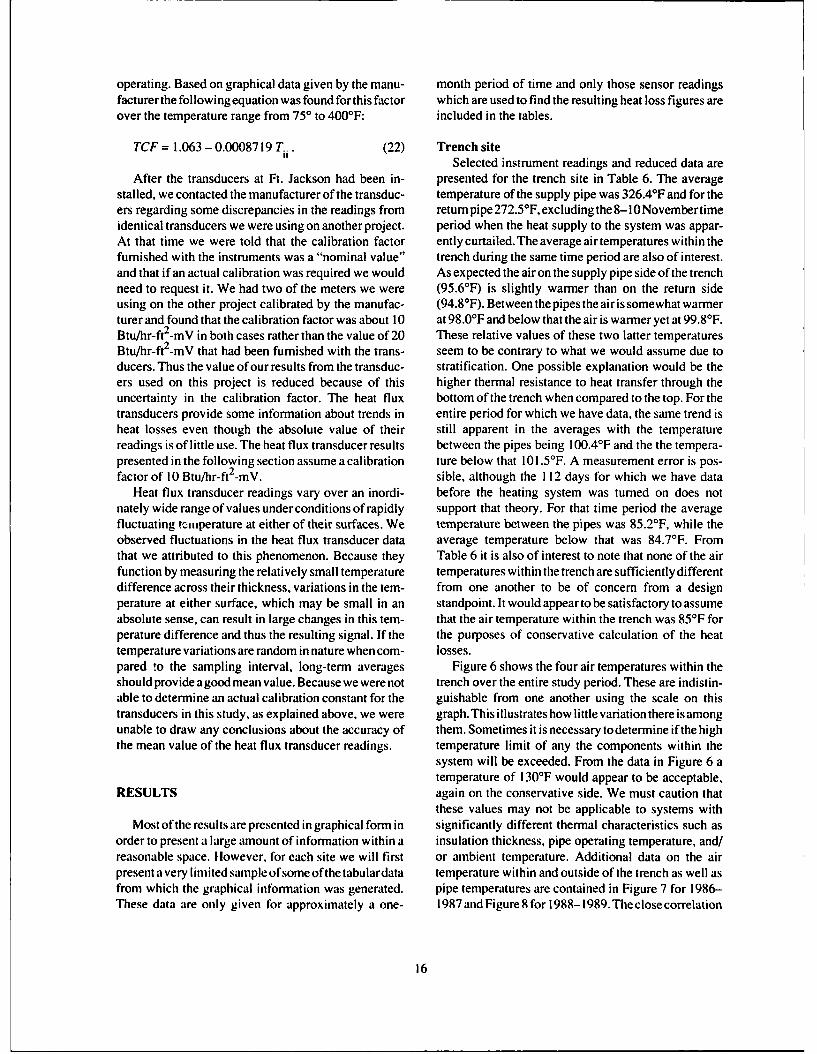
operating. Based on graphical data given by the manu- month period of time and only those sensor readingsfacturer the following equation was found for this factor which are used to find the resulting heat loss figures areover the temperature range from 750 to 400'F: included in the tables.

TCF = 1.063 - 0.0008719 T... (22) Trench siteSelected instrument readings and reduced data are

After the transducers at Ft. Jackson had been in- presented for the trench site in Table 6. The averagestalled, we contacted the manufacturer of the transduc- temperature of the supply pipe was 326.4°F and for theers regarding some discrepancies in the readings from returnpipe272.5°F, excludingthe8-10Novembertimeidentical transducers we were using on another project. period when the heat supply to the system was appar-At that time we were told that the calibration factor ently curtailed. The average air temperatures within thefurnished with the instruments was a "nominal value" trench during the same time period are also of interest.and that if an actual calibration was required we would As expected the air on the supply pipe side of the trenchneed to request it. We had two of the meters we were (95.6°F) is slightly warmer than on the return sideusing on the other project calibrated by the manufac- (94.8°F). Between the pipes the air is somewhat warmerturer and found that the calibration factor was about 10 at 98.0°F and below that the air is warmer yet at 99.8°F.Btu/hr-ft2-mV in both cases rather than the value of 20 These relative values of these two latter temperaturesBtu/hr-ft2-mV that had been furnished with the trans- seem to be contrary to what we would assume due toducers. Thus the value of our results from the transduc- stratification. One possible explanation would be theers used on this project is reduced because of this higher thermal resistance to heat transfer through theuncertainty in the calibration factor. The heat flux bottom of the trench when compared to the top. For thetransducers provide some information about trends in entire period for which we have data, the same trend isheat losses even though the absolute value of their still apparent in the averages with the temperaturereadings is of little use. The heat flux transducer results between the pipes being 100.4°F and the the tempera-presented in the following section assume a calibration ture below that 101.5°F. A measurement error is pos-factor of 10 Btu/hr-ft2-mV. sible, although the 112 days for which we have data

Heat flux transducer readings vary over an inordi- before the heating system was turned on does notnately wide range of values under conditions of rapidly support that theory. For that time period the averagefluctuating tciiperature at either of their surfaces. We temperature between the pipes was 85.2°F, while theobserved fluctuations in the heat flux transducer data average temperature below that was 84.7°F. Fromthat we attributed to this phenomenon. Because they Table 6 it is also of interest to note that none of the airfunction by measuring the relatively small temperature temperatures within the trench are sufficiently differentdifference across their thickness, variations in the tem- from one another to be of concern from a designperature at either surface, which may be small in an standpoint. It would appear to be satisfactory to assumeabsolute sense, can result in large changes in this tem- that the air temperature within the trench was 85°F forperature difference and thus the resulting signal. If the the purposes of conservative calculation of the heattemperature variations are random in nature when com- losses.pared to the sampling interval, long-term averages Figure 6 shows the four air temperatures within theshould provide agood mean value. Because we were not trench over the entire study period. These are indistin-able to determine an actual calibration constant for the guishable from one another using the scale on thistransducers in this study, as explained above, we were graph. This illustrates how little variation there is amongunable to draw any conclusions about the accuracy of them. Sometimes it is necessary to determine if the highthe mean value of the heat flux transducer readings. temperature limit of any the components within the

system will be exceeded. From the data in Figure 6 atemperature of 130°F would appear to be acceptable,

RESULTS again on the conservative side. We must caution thatthese values may not be applicable to systems with

Most of the results are presented in graphical form in significantly different thermal characteristics such asorder to present a large amount of information within a insulation thickness, pipe operating temperature, and/reasonable space. However, for each site we will first or ambient temperature. Additional data on the airpresent a very limited sample of some ofthe tabulardata temperature within and outside of the trench as well asfrom which the graphical information was generated. pipe temperatures are contained in Figure 7 for 1986-These data are only given for approximately a one- 1987 and Figure 8 for 1988-1989. The close correlation

16

0 0.00-C 0C0P~' "m 0.0D- 0.00. 0. 0.gOlG

04., L^ 0Nl: tL MMin P-INW n70. Y0 N 0 ' 0 1 cm -%QNOom c

U) n N in% WN iN Wn V% WN in W in% in i in in in in in in in in WN in in WN W% in W% i

c nf 0 ni I4*. 0 It I uL AV lW w %V %in n N N

go.4 L o 'a ' in 'o 0100100 010 101,01 c

V-n!c9 msn 000-N rnmt- 10c onri rns N niF' in G N

-Q L3U '0n' ' 'o O n n LMM In LM

Cu U) ( - -- -

Q.5- 0 m N G n'0 1 iniC(Dn9-.0 ''U i 0It PIt n imnICu U g..-O. 0..006 s8 0.i & 00 W) 0 U 00, 0. l .0-0 0. 00-0. 0. 0. 0.

-:W 6 ' 3, V().LA t -* t'-*ON '0j N.*~''N -!S -* ) Y P

1 L6

0., -' n.' -! 0l gg9'0:7

U~~~~~ OCr.-00oo0-.-00& 0 ,,,00 0-r.-r

.. 0. . . . . . ... . .0. '*n. .O. .0 . . . . . . .

61 0L4

m 41 .- 00000 0.0a04DUo0.0.0a.a, 0.0. c. 0.0.0.C>0. 0. 0.

LU .. -u

417

Trench Air TemperaturesInside trench only140 T

120

80 Figure 6. Trenchair temperaturea I over the studyE 60

I- period.

40

20

0 ; i I I1986 1987 1988 1989

Shallow trench temperaturesDaily averages for 1986

350 -300 Supply pipe

",Return pipe~250

. 200

E 150Trench air

10050 Outside air

0 I I . I I I I I I I

J F M A M J J A S 0 N D

Shallow trench temperatures Figure 7. TrenchDaily averages for 1987 temperatures for

350 1986-1987.

300 Supply pipe

250

e 200

150 Return pipe

100 T Trench air

50 Outside air

0 I I I I I I I, I

J F M A M J J A S 0 N D

18

Shallow trench temperatures

350 Daily averages for 1988

300Supply pipe

C 250 Return pipe

. 200

12 100.. Trench air

50 --W kOutside air00. 0

SF M A M J J A S 0 N D

Shallow trench temperatures

400 Daily averages for 1989

350 . Supply pipe® 300 .. ,t .

5 250 "Vl1 " ' Return pipe

C200E150

e M100 A - hlo t t uTrenchair50 ,,,W , / V v Outside air

J F i A M J J A S 0 N D

Figure 8. Trench temperatures for 1988-1989.

of trench temperature variations to ambient air tempera- tern was apparently curtailed for some time during theture variations is obvious in these figures. This is a 8-10 November period as we noted above. If we exam-manifestation of the relatively small thermal resistance ine the average heat loss exclusive of this time period,between the trench interior and the environment which we see that the average is slightly higher at 96.0 Btu/hr-the trench lid provides. In extreme cold climates sub- ft. Figure 9 shows the heat loss from the shallow trenchfreezing temperatures within such a system are pos- for the entire study period. The reduction in heat lossessible. Heat tracing and/or insulation of the trench from during 1988 and 1989 over the previous years is attrib-the environment may be necessary in such cases. For utable to the reduced return temperature during thatadditional information on such designs we refer the time period. This is a fairly significant reduction andreader to Phetteplace et al. (1986) and Kennedy et al. provides a clear example of the benefits of keeping the(1988). temperature differential between supply and return as

Because the heat flux transducer readings were of large as possible, thus resulting in lower return tempera-limited valueasexplainedinthesectionabove, onlyone ture. Not only will heat losses be reduced by lowermethod of computing the heat loss is available for this return temperatures, but pumping costs are also reducedsite. For the month of November 1986 the average heat since less mass will need to be circulated. Of course, thisloss from the trench system was 90.2 Btu/hr-ft. This is assumes that the thermal load is constant and that somesomewhat misleading since the heat supply to the sys- method of reducing pumping power input, such as

19

110 IT F - -I I I I I-TI I I 71"1-r I 1 I I I I I

100 -

E

70

60

50

OIN D IFIMA MJ JA SON FMAM J J J F M A M J

1986 1987 1988 1989

Figure 9. Heat losses for the trench site over the study period.

80-

60-1C _supply

40-

rn

20-I I

1986 1987 1988 1989 1990

Figure /0. Heatflux sensor data for the trench site.

variable speed drives or multiple pumps, is available. Common conduit siteHeat flux sensor output is shown in Figure 10. Here Table 7 contains selected raw and reduced data for

the sensor output has been averaged over 10-day peri- the common conduit site. As with the data forthe trenchods to attempt to eliminate the oscillations which occur site, averages have been compiled that exclude thein the daily average data. A calibration factor of 10 Btu/ period of 8-10 November during which the heat supplyhr-ft-mV has been assumed. The general agreement to the system was apparently turned off. The tempera-between the total loss of the supply and return pipes as ture of the supply during the period summarized indetermined by the heat flux sensors and the insulation Table 7 averaged 325.3°F and the return averagedmethod (Fig. 9) is reasonable using this calibration factor. 256.8°F for the same period of time. The supply tem-

20

400 I I

Supply300 - Pipe y---

MReturn= 200 Pipe

r1 , Conduit.-

-' ",,-Ground _

0 .I I I

1986 1987 1988 1989 1990

Figure I. Common conduit site temperatures.

perature is very close to the supply temperature ob- The heat losses for the entire study period for theserved at the trench site, which is reasonably close to common conduit site are shown in Figure 12 for 1986-this site. The return temperature averaged about 16'F 1987 and Figure 13 for 1988-1989. Note that during thelower at this site when compared to the trench site. This early spring (around March), for each of the three yearswould tend to make heat losses lower at this site if all that we have data during this time period, the results

else were equal, as of course is not the case. The from the insulation method increase to a value greatertemperature of the outer surface of the conduit averaged than those for the soil method. Some time during the fall131.7'F while the undisturbed ground temperature at (about mid-September for 1987, the only year for whichapproximately the same depth as the centerline of the we have data during this time period) the trend isconduit averaged 63.6'F. This illustrates the rather dra- reversed. One possible explanation for this is the soilmatic effect which the buried conduit has on surround- moisture content. The data in Table 4 suggest that theing soil temperatures. Figure I I shows the temperatures soil moisture content is higher during the spring anddiscussed above for the entire study period. summer than in the winter. If the moisture content of the

The heat losses for the common conduit system were soil around the conduit, particularly that between thecalculated by three of the methods described earlier, conduit and the ground surface, increases during theexclusive of the heat flux transducer method. The method spring and summer months, then the thermal conductiv-referred to as the "soil method" uses the single buried ity of the soil will increase during that time period aspipe equation presented earlier and the conduit outer well. This will reduce the thermal resistance of the soilsurface temperature to calculate the heat flow. The in an absolute sense as well as relative to the otherthermal conductivity of the soil is taken as 7.5 Btu-in./ thermal resistances in the system.hr-ft -F (0.625 Btu/hr-ft-°F) in this and the CEGS- Presumably the other thermal resistances remain02695 method. This is felt to be a realistic average value fairly constant year-round, notably the insulation ther-based on the observed soil type and moisture content mal resistance, which is much greater than the thermaland published data (Kersten 1949). resistance of the soil or any other thermal resistance in

The average of the values computed by the three the system. Thus, the overall thermal resistance will bemethods is 114.1 Btu/hr-ft. The highest of the methods reduced by a much smaller relative amount than the soil(CEGS-02695) was approximately 7.3% greater than thermal resistance. With the lower thermal resistancethe average value and the lowest (Insulation method) the temperature drop across the soil from the conduitwas 5.8% below the average. Considering the diffi- casing to the ground surface will decrease relative to theculty involved in making thermal measurements of this other temperature drops in the system. However, wenature, we feel this agreement is very good. This is have assumed that the thermal conductivity of the soilparticularly true when one considers that the CEGS- is constant year-round in our soil method and thus, with02695 method has conservative assumptions (in that the lower actual resistance and relative temperaturethey would underpredict the actual thermal re- drop measured, we will underpredict the heat flow. Wesistance) regarding the heat transfer across the air are continuing to take temperature data at this site andspace. plan to take additional soil moisture data as well. Once

21

fn:- 4C4mnr 00 n fn 0 0i~ Fn ~ 0pn ~ ~ U% Cc -LN41 6. - - -

0 r' 0O '~ * - 1 Pl0 0 - b N

- .0

c-~~wrwN QP in inni C4i jF A L %U N 0 on

0 do 0 . .- r 0

410

z 't NybOP-IN f-ON 40y Nyb IN I'N 0yb it1 MCMninC nC 'r - N 0'LO 0o ~ t #ov3 orL*'o-

0%- C UO in 0 4O 0 N -Go'tMC0 -N 0 O '0 N l 4MrCP . t 1%D 4- A Nn - r I r -S11ItI t- % ft1 1 4rt It s

041p .0I= >. " -t & Mr ;;;;R ? ; N e r 40'No-' Q000 Q

U It 19 . ini . *'0't'-''0'0000N0'.' NNN

l. C a-o1 101 1 tI 10'0'0'0 0 -*'00'00 t ^. '. 0 - 0 10 0 0 o n '0 '0I- Ye I i t NNNNNNNNNNNNNNNNNNNNNNNNNNNNNcmcmcm m li m y C NrN N Nm

C,.aaQ 4Ca C3. a 0000000000000000000000000 000 0 C 0

to 1L- '4-

3. -4Uy% NPNP cm cmmmmmN mm m mm...I

*00UN 4INO tn CC Q 0 N a . cm m.trst ON

101 N-0 r- % 100 Ni0 yb kn 010 0 0 0 0' N, iMnAa

C Ln 410 '0 4 0 NPm '0N1"-m0N 0Itnni0 '0.0 ,% %0 M

0.1 Cn * tn 0' 00 ! Oy P-0N N N 0l sr m '0 '0'N in a 0' Ln. .10: W!

0.1a n10 4-1 -4 10n0iii NyrO 0 :83OON'0'0'0 0 10'--00 0-. -r -rrr -rrrrrrrrrrrrrrrra-r-

v N4O N 'ieN o0O'n %0 00 Om w -S b r'0O inoro y N N%U Go ~ r O' -*' ^Oy ino unin-; taNAin WVt I 't

o - C M0' Go00000'''''

* ' Ok'40P-r.%NO 0 PNNt0M&A nOOinN'0NininsP. t tnO P,400- P, CMkrN- vc jr 0 l cjMc % - cmcmc OP-mO. ru-O tv' '00 0y ru ̂ A NCY As N0' 0y '0 r

L1410.41 l lFnwlw w w m m Fn M m P- Mi' onyyi'i~--tt0n n 4 m inm

0 - l NNNNNNNNNN0. NNNNNNNNMNNNN N, Nn W Igcc0~~~~~~~~~l in1NO-0n O-*OO.N0~n0 0 0

00 0 0 00 0c c

T .I .I TF77I -;- . iF. I T . r r T-.L rymg( n0P Aa 4M' %ON0 0 1 w-

coo 0 --- M i AG

22

20I I I CEGS-02695

Qsoil 7.510 0 k- I °nI "

- 1986 Insulation0 I . , I

~160.216 , d,,(EGS=.0269S3n

120 -

8 Osoil 7.5 Insulation

401987

0 i L I i i I i i iJ F M A M J J A S O N D

Figure 12. Common conduit site heat loss for 1986-1987.

we have more data we will attempt to adjust the soil trench/soil in the case of the shallow trench. It is difficultmoisture content and thermal conductivity used in our to make precise comparisons because the insulationcalculation on a seasonal basis to more accurately thicknesses vary for the two sites. If, however, wemodel this effect. compare the effective thermal resistance between the

Study of the outer conduit temperature and the tem- average insulation surface temperature and the ambientperature forthe corresponding time period forthe trench air temperature, we find that it is 34 % lower (0.55 hr-interior gives some indication of the thermal resistance ft-°F/Btu) for the trench than for the common conduitprovided by the soil for the buried conduit, in compari- (0.84 hr-ft-°F/Btu). Thus the burial depth of the conduitson to the lesser thermal resistance provided by the provides additional thermal resistance over the trench

160 1 i 1 1 1 1 I 1 1CEGS - 02695

120 - I * Insulation

1 t soil7.580-

401988

16 0 i I I I i i I I I

160

120 C EGS - 02695

4e Insulation80 0 soil 7.5

40 1989

0 I I I I I I I I I IJ F M A M J J A SO N D

Figure 13. Common conduit heat loss for 1988-1989.

23

system with its top cover at grade level. The trench than the lowest (CEGS-02695 method). Again, consid-system, however, can accommodate incrementally ering the difficulty involved in making thermal mea-thicker insulation at much lower cost than the conduit surements of this nature we feel this agreement is verysystem. good. The heat losses for the entire study period for the

individual conduit site are shown in Figure 16.Individual conduit site Figure 17 shows the heat flux sensor data for the

Table 8 contains selected raw and reduced data for study period at the individual conduit site. The sensorthe individual conduit site. The temperature of the data have been averaged over 1 0-day periods in Figuresupply during the period summarized in Table 8 aver- 17 in order to eliminate the wide fluctuations that areaged 348.5°F and the return averaged 203.4°F for the found in the readings, as discussed earlier. The calibra-same period of time. The temperature of the outer tion factor has been assumed to be 10 Btu/hr-ft -mV assurface of the conduit averaged 73.81F for the supply before. With this calibration factor the agreement be-and 71.7°F for the return. The undisturbed ground tem- tween the heat losses predicted by this method and theperatureat approximately the samedepthasthecenterline results of the other two methods shown in Figure 16 isof the conduit averaged 50.3°F. Here the temperature fairly good.difference between the outside of the conduit and the Earlier when introducing eq 5 we noted that theundisturbed soil temperature at the burial depth is only thermal resistance of the air space is currently base5 on21 .4°F. This can be compared to a temperature differ- an assumed heat transfer coefficient of 3 Btu/hr-ft -'Fence of nearly 60°F at the common conduit site. The where the surface area is that of the insulation's outerprimary reason for this much lower temperature differ- surface. From our data we can calculate an observedence at the individual conduit site is the increased value for this heat transfer coefficient. This can be doneinsulation thickness at that site. Because the thermal by combining the equation for the resistance of the airresistance of the insulation is much larger at the indi- gap, eq 5, with the definition of this resistance to get thevidual conduit site, the thermal resistance of the soil following equation:becomes a much smaller fraction of the total and thusthe corresponding temperature drop across that resis- qtance decreases. I = (22)

Figure 14 shows the temperatures discussed above 2n rio (Tio - Too)forthe entire study period. At the individual conduit sitea data logging system separate from that used at the where h = the equivalent heat transfer coefficient ofother two sites is used. The control string of thermo- the air space based on the outer surface area of thecouples, which gives undisturbed ground temperatures, insulation (Btu/hr-ft -°F).

is connected to the data logging system for the common This expression neglects the thermal resistance ofconduit and trench sites. This has presented an unusual the steel conduit, which is a reasonable assumption indifficulty in reducing the data for the individual conduit most cases. We have also used the heat flow as mea-site because the data logging system at this site was sured with the insulation method described earlier, asoperational during some periods when thedata loggerat this was felt to be the most reliable of the methodsthe other site was not. In order to obtain the control data used.on undisturbed soil temperatures at the individual con- Equation 22 was used to calculate ha for 626 sets of• asduit site, we used least squares techniques to fit a daily averages for the data. For the supply conduitsinusoidal curve to all of the control string data we had system the mean value ofh asw 1.15 Btu/hr-ft 2 -F withfrom the data logger at the other two sites. Figure 15 the standarddeviationbeing . 1lOBtu/hr-ftl-°F.Fortheshows the resulting curve and the average of all avail- return conduit system the mean value was 1.51 and theable temperature data. standard deviation was 0.225. These values woud tend

The heat losses for the individual conduit system to indicate that the assumed value of 3 Btu/hr-ft -*F iswere calculated by the insulation and CEGS-02695 higherthan those experienced in practice, at least in thismethods described earlier. As in the calculations for the case. More data are needed from other system configu-common conduit site, the therryal conductivity of the rations, however, before sufficient justification for low-soil wastaken as7.5 Btu-in./hr-ft -FfortheCEGS-02695 ering this value would exist. If the results of this studymethod. are representative, the current factor is conservative in

The average of the heat loss values computed by the that it would underpredict the thermal resistance of thetwomethodsis78.8Btu/hr-ft.Thehighestofthemeth- air space and thus the heat transfer would beods (Insulation Method) was approximately 9.3% greater overpredicted.

24

0- .. 2N in-i 09 O9 1 NNVn.a c eI N cl c9r9e99rrr * c) z1.r22rz fA

00, 4- 990 971 , 7 n 9V 79P :1 1

Nih m~" N" m

u~~~~~~ C ~~ ~ I 0 O N 0 - O- i in t * - 0N ' .C -mM FA

A~ k.C 0n UN inL nN Nk NL %9 %W tW %b n6%I n6 ni nWI-0~nNN N N N N N N t J N N f J

PL0!4-O0it .0L ;;gL; s

0- 020 70 0N . * O . NoZZ ZG' o Coo w m d 0 G

z n a o o& N ae i ntyc *'oo o oc~ .c w%- PN N . o. t-

So " 4W ; ;1 *** , **,*,*,****,, ,,, ,.2-A :.cItI I pIN.0 1 nN a 'AO * t ra wa 01 V%evC Y Y

2 -am,. - P ~ .N 0*N V V 1- n-~-

. ~ ~ N -,Q 0, 0 0 0 0 N NNO f00000 woPo0 Ikn &^L 1W %W V %V ni n'r ni ni %gni %0 %V %w NW % L

It It4-rI tI tI rItI tI 11" tI tIt n6 ni tt ^ %1.4 1. *VI "A"NN"

N It( (D0L4- !1 W W0) Go0 . 6c oNNNG oG .o0 0 O C )C %W NL 3

= oWa %. ,. tI I tI tI tI t0 It .4 W%.. 0O 0 O0N0N 0 WN I-t % O-*.. 1in '0. &nW '0U i

C ~ ~ Ll,, PI N0'0'0 11! .1% W! ,ininnOnD'

0- -. P1 2PPP r I i4iiiiiiiiiiiiiiiiiiiiiiiiiii in " " N

C! -2 - NNz NN NNN NN NNNNNNNNzN24;z N"N NNu~ t 4) 000 9 00 00 000-

40 c 0

3 3 00) >n 0.t4> *0 t.*itoo Go.GonGoiNiN C 0 NiNinn n i

c~

C'V .- N NN0N'ii t;'0 0O0.. N 0in N

NL1,4 NNN N 0.N..NN 0-. ~CW'.M MNN NMNNMN NMinONNN NN NN. N It

.= L00I-- l0 0 l0 0 0 0 0 lO l 0 lO l 0 0 lC00 ,E~.. Nn'N~ 0 N NiN'000.coV

CL1' 1 4911O r! '%0 0 0 C n1 r U .0 %'4 909 91N n 900:

R3 0- M MN"NmNmNM NNNN N 0 N N N 0 0 0 0 NM" )m"(J0)C0 .0 o 0 ( >0 ) l0 0 0 0 l l0 lO 0 C 0 o

C 02 . C 000NN 0 0 O 0 i n N O00~ n 0 . ~ 0? ~ . . ?C ? V

- IL00 0 000.0Q0v000 0 NONNN.1.,'Om inm0

LMON)O l '46N20 -N I? C6 >IOL 06 - -- -- - -- CY~cvjcjtj N ~ oQ ~~ o

.000...000...000....00OO00f.L25LL L L

1988289

-,400 SPp

I20 Ground

0

J F MA MJ J ASO0N DJ F MA MJ

Figure 14. Individual conduit site temperatures.

00

60 -Bs i

E 2o 20

Figure 15. Average undisturbed soil temperature at 74 in. andfitted sinusoidal curve.

100 I I I

90

80 -Total Insulation j' A Ai

70 - Total CEGS - 02695

60

E~50

Supply Insulation-J V' d '

40 - Supply CEGS -02695

Return Insulation r,130- Return CEGS - 02695

20-

1 MajArMay Jun Jul Aug Sep Oct Nov DcJan F 1 Mar Apr1 May J

1988 1989

Figure 16. Individual conduit site heat losses.

26

60 1 1 1

50

supply

'. 40

Return

30

20-

J F M A M J J A S 0 N D J F M A M J J

Figure 17. Heat flux sensor data for the individual conduit site, 10-dayaverages.

CONCLUSIONS reduced significantly for this extended monitoring pe-riod. Because the data logging systems are currently in

Much of the data taken on this project has not yet place and operating satisfactorily we are continuingbeen reduced. This is particularly true of the extensive data acquisition as described earlier. We currently havesoil temperature data, which have been gathered around approximately one year of additional data at all the sitesthe three types of systems. We plan to analyze these data beyond that presented here. This is information cur-numerically using finite element methods. A small rently being reduced and will be published in a futuresample of data from this project was analyzed in this comprehensive report on the project.way by Fleck (1989). We plan to expand both theamount of data analyzed and the methods used.

The results from the data that have been reduced are LITERATURE CITEDvery encouraging. We feel that two of the major objec-tives of the study have been accomplished: CSCE (1986) Cold Climate Utilities Manual. Canadian

1. We have shown that heat losses can be measured Society for Civil Engineering, Montreal, Quebec.by several different methods with reliable and Fleck, B.H. (1989) Heat loss from buried pipes. Masterrepeatable results. of Science Thesis (unpublished), Thayer School of

2. We have established the level of heat losses from Engineering, Dartmouth College.three types of operating heat distribution systems Kennedy, F.E., G. Phetteplace, N. Humiston and V.under field conditions. Prabhakar (1988) Thermal performance of a shallow

At this point three other objectives remain: utilidor. In Proceedings of the Fifth International Per-1. To determine the long-term thermal performance mafrost Conference, Trondheim, Norway, vol 2, pp.

of these heat distribution systems. 1262-1267.2. To analyze the soil temperature data more exhaus- Kersten, M.S. (1949) Laboratory research for the de-

tively to determine if heat losses can be accurately termination of the thermal properties of soils. Engineer-predicted using such information. ing Experiment Station, University of Minnesota.

3. To determine if the existing calculational methods Lunardini, V.J. (1989) Measurement of heat lossesand assumptions are valid or if they are in need of from aconduit-type heat distribution system. USA Coldmodification. Regions Research and Engineering Laboratory, Pre-

In order to determine the long-term performance of liminary Report (unpublished).the systems we would like to continue monitoring them Lunardini, V.J. (1990) Measurement of heat lossesforat least 10 more years. This would provide almost 15 from a conduit-type heat distribution system. Paperyears worth of data on the trench and common conduit presented at the 1990 Army Science Conference (ASC),site. The amount of data being collected could be Durham, N.C.

27

Phetteplace,G., P. Richmond and N. Humiston (1986) Segan, E.G. and C. Chen (1984) Investigation of tri-Thermal analysis of a shallow utilidor. In Proceedings service heat distribution systems. Technical Report M-of the International District Heating and Cooling 347, USA Construction Engineering Research Labora-Association, Washington, D.C., pp. 61-69. tory, Champaign, Illinois.Phetteplace, G. (1990) Low temperature hot water heat U.S. Army (1988) Facilities Engineering and Housingdistribution systems. Facilities Engineering Applica- Annual Summary of Operations. Volume Il-Installa-tions Program (FEAP) Fact Sheet, USA Cold Regions tions Performance. Office of the Assistant Chief ofResearch and Engineering Laboratory. Engineers, Department of the Army.Phetteplace, G. and V. Meyer (1990) Piping for ther- U.S. Army Corps of Engineers (1989) Undergroundmal distribution systems. CRREL Internal Report 1059 Heat Distribution Systems (Preapproved Systems).(unpublished), USA Cold Regions Research and Engi- CEGS 02695, USA Corps of Engineers, Washington,neering Laboratory. D.C.

28

APPENDIX A: SENSOR LOCATIONS

Two pipes, single conduit, C-site.

Channel Outputno. Label units Location

0 AIR/C-SITE TREE F Air temperature, located on side of tree.I C-SITE TOP PIPE F Attached to top of supply pipe.2 C-SITE BTM PIPE F Attached to top of return pipe.3 C-SITE TOP INS F Attached to top of supply pipe insulation.4 C-SITE BTM INS F Attached to top of return pipe insulation.5 C-SITE TOP AIR F Air temp. inside conduit above pipes.6 C-SITE BTM AIR F Air temp. inside conduit below pipes.7 C-SITE MID AIR F Air temp. inside conduit between pipes.8 C INNER SURFACE F Att'd. at 45 deg. to inner surf. of conduit.9 C CTR STR Y=2.0 F Gnd temp. 2 in. from surf. above center of pipe.

10 C CTR STR Y=7.0 F Gnd temp. 7 in. from surf. above center of pipe.11 C CTR STR Y= 13 F Gnd temp. 13 in. from surf. above center of pipe.12 C CTR STR Y=19 F Gnd temp. 19 in. from surf. above center of pipe.13 C CTR STR Y=25 F Gnd temp. 25 in. from surf. above center of pipe.14 C CTR STR Y=37 F Gnd temp. 37 in. from surf. above center of pipe.15 C CTR CDT TP 44 F Top outside surf. of conduit, 44 in. from surface.16 C CTR CDT TP 44 F Top outside surf. of conduit, 44 in. from surface.17 C OUTER SURFACE F Attached to outer surface of conduit.18 HFS TOP PIPE mV Heat flow sensor attached to the top pipe.19 HFS BOTTOM PIPE mV Heat flow sensor attached to bottom pipe.20 C2 STG Y=9.0 F Gnd temp. 9 in. from surf. I'l l in. from ctr. cond.21 C2 STG Y=14 F Gnd temp. 14 in. from surf. I'll in. from ctr cond.22 C2 STG Y=20 F Gnd temp. 20 in. from surf. I'l I in. from ctr cond.23 C2 STG Y=26 F Gnd temp. 26 in. from surf. I'I in. from ctr cond.24 C2 STG Y=32 F Gnd temp. 32 in. from surf. I I! in. from ctr cond.25 C2 STG Y=44 F Gnd temp. 44 in. from surf. I' 11 in. from ctr cond.26 C2 STG Y=56 F Gnd temp. 56 in. from surf. I'l I in. from ctr cond.27 C2 STG Y=68 F Gnd temp. 68 in. from surf. I'l l in. from ctr cond.28 C2 STG Y=80 F Gnd temp. 80 in. from surf. I'l l in. from ctr cond.29 C2 STG Y=92 F Gnd temp. 92 in. from surf. I'l l in. from ctr cond.30 C2 STG Y= 104 F Gnd temp 104 in. from surf. 1. 11 in. from ctr cond.31 C2 STG Y=104 F Gnd temp 104 in. from surf. 1.11 in. from ctr cond.32 DATA LOGGER BOX F Temperature inside data logger storage box.

29

Two pipes, concrete trench, T-site.


100 T-BTM CTR AIR F Air temperature inside, trench, lower center.101 T-LH WALL CTR F Inside trench wall, return side, at mid-height.102 T-RT PIPE F Attached to supply pipe.103 T-LH PIPE INS F Attached to top of return pipe insulation.104 T-CTR AIR F Air temp.between supply and return pipes.105 T-LH PIPE F Attached to return pipe.106 T-RH PIPE INS F Attached to top of supply pipe insulation.107 T-LID UNDERSIDE F Attached to underside of trench cover.108 T-FLOOR CTR F Attached inside trench to center of floor.109 T-RH WALL CTR F Inside trench wall, supply side, at mid-height.110 T-AIR LT OF LP F Air temp. inside trench, left of return pipe.111 T-AIR RT OF RP F Air temp. inside trench, right of supply pipe.112 T-CTL Y=3.0 F Gnd temp., 3 in. from surface, 13.2' from trench.113 T-CTL Y=8.0 F Gnd temp., 8 in. from surface, 13.2' from trench.114 T-CTL Y=14.0 F Gnd temp., 14 in. from surface, 13.2' from trench.115 T-CTL Y=26.0 F Gnd temp., 26 in. from surface, 13.2' from trench.116 T-CTL Y=38.0 F Gnd temp., 38 in. from surface, 13.2' from trench.117 T-CTL Y=56.O F Gnd temp., 56 in. from surface, 13.2' from trench.118 T-CTL Y=74.0 F Gnd temp., 74 in. from surface, 13.2' from trench.119 T-CTL Y=98.0 F Gnd temp., 98 in. from surface, 13.2' from trench.120 TI STG Y=2.0 F Gnd temp., 2 in. from surface, 2.4' from trench.121 TI STG Y=7.0 F Gnd temp., 7 in. from surface, 2.4' from trench.122 TI STG Y=13.0 F Gnd temp., 13 in. from surface, 2.4' from trench.123 TI STO Y=25.0 F Gnd temp., 25 in. from surface, 2.4 from trench.124 TI STG Y=37.0 F Gnd temp., 37 in. from surface, 2.4' from trench.125 TI STG Y-49.0 F Gnd temp., 49 in. from surface, 2.4' from trench.126 TI STG Y=6 1.0 F Gnd temp., 61 in. from surface, 2.4' from trench.127 TI STG Y=68-CWP F Gnd temp., 68 in. from surface, 2.4' from trench.128 T6 STG Y=2.0 F Gnd temp., 2 in. from surface, 6.7' from trench.129 T6 STG Y=7.0 F Gnd temp., 7 in. from surface, 6.7' from trench.130 T6 STG Y= 13.0 F Gnd temp., 13 in. from surface, 6.7' from trench.131 T6 STG Y=25.0 F Gnd temp., 25 in. from surface, 6.7' from trench.132 T6 STG Y=37.0 F Gnd temp., 37 in. from surface, 6.7' from trench.133 T6 STG Y-49.0 F Gnd temp., 49 in. from surface, 6.7' from trench.134 T6 STG Y=61.0 F Gnd temp., 61 in. from surface, 6.7' from trench.135 T6 STG Y=73.0 F Gnd temp., 73 in. from surface, 6.7' from trench.136 T-HFS LH PIPE mV Heat flow sensor attached to return pipe.137 T-HSF RH PIPE mV Heat flow sensor attached to supply pipe.139 T-AIR IN MNHOLE F Air temperature inside man hole w/extender.

30

Two pipes, individual conduits, S-site.


100 SITE2-OUTSD AIR F Air temperature located on side of tree.101 SITE2-MANHL AIR F Air temperature inside man hole.102 SUPPLY(S) HFS mV Heat flow sensor attached to supply pipe.103 RETURN(R) HFS mV Heat flow sensor attached to return pipe.104 S-TOP CAR.PIPE F Attached to top of supply carrier pipe.105 S-TOP INSUL F Attached to top of insulation on supply pipe.106 S-BOT INSUL F Att'd to bot. of insulation on supply pipe.107 S-TOP AIRSPACE F Air temp. in space above supply carrier pipe.108 S-MID AIRSPACE F Air temp. in space beside supply carrier pipe.109 S-BOT AIRSPACE F Air temp. in space below supply carrier pipe.110 S-TOP INSD COND F Attached to top inside of supply conduit.III S-BOT INSD COND F Attached to bottom inside of supply conduit.112 R-TOP CAR. PIPE F Attached to top of return carrier pipe.113 R-TOP INSUL F Attached to top of insulation on return pipe.114 R-BOT INSUL F Att'd to bot. of insulation on return pipe.115 R-TOP AIRSPACE F Air temp. in space above return carrier pipe.116 R-MID AIRSPACE F Air temp. in space beside return carrier pipe.117 R-BOT AIRSPACE F Air temp. in space below return carrier pipe.118 R-TOP INSD COND F Attached to top inside of return conduit.119 R-BOT INSD COND F Attached to bottom inside of return conduit.120 S-ON COND, RGHT F Attached outside, rightside of supply conduit.121 S-ON COND, TOP F Attached outside, top of supply conduit.122 S-ON COND, LEFT F Attached outside, leftside of supply conduit.123 S-ON COND, BOT F Attached outside, bottom of supply conduit.124 R-ON COND, RGHT F Attached outside, rightside of return conduit.125 R-ON COND, TOP F Attached outside, top of return conduit.126 R-ON COND, LEFT F Attached outside, leftside of return conduit.127 R-ON COND, BOT F Attached outside, bottom of return conduit.128 Z-Q CBL/21N F Gnd-temp. 2 in., 30 in. rt. of return pipe center.129 Z-Q CBL/121N F Gnd-temp. 12 in., 30 in. rt. of return pipe center.130 Z CBL/231N F Gnd-temp. 23 in., 30 in. rt. of return pipe center.131 Z CBL/35IN F Gnd-temp. 35 in., 30 in. rt. of return pipe center.132 Z CBL/471N F Gnd-temp. 47 in., 30 in. rt. of return pipe center.133 Z CBL/591N F Gnd-temp. 59 in., 30 in. rt. of return pipe center.134 Z CBL/7 I IN F Gnd-temp. 71 in., 30 in. rt. of return pipe center.135 Z CBL/831N F Gnd-temp. 83 in., 30 in. nt. of return pipe center.136 Z CBL/951N F Gnd-temp. 95 in., 30 in. rt. of return pipe center.137 Z CBL/l 191N F Gnd-temp. 119 in.. 30 in. rt. of return pipe center.138 Z CBL/1431N F Gnd-temp. 143 in., 30 in. rt. of return pipe center.139 Z CBL/179IN F Gnd-temp. 179 in., 30 in. rt. of return pipe center.140 Y-Q CBL/2IN F Gnd-temp. 2 in., on center line of return pipe.141 Y-Q CBL/61N F Gnd-temp. 6 in., on center line of return pipe.142 Y CBL/121N F Gnd-temp. 12 in., on center line of return pipe.143 Y CBL/1 81N F Gnd-temp. 18 in., on center line of return pipe.144 Y CBL/28IN F Gnd-temp. 28 in., on center line of return pipe.145 Y CBL/40IN F Gnd-temp. 40 in., on center line of return pipe.146 Y CBL/521N F Gnd-temp. 52 in., on center line of return pipe.147 Y CBL/581N F Gnd-temp. 58 in., on center line of return pipe.148 Y CBL/64IN F Gnd-temp. 64 in., on center line of return pipe.

31

Two pipes, individual conduits (cont'd).


149 Y CBL/70IN F Gnd-temp. 70 in., on center line of return pipe.150 Y-S CBL/921N F Gnd-temp. 92 in., on center line of return pipe.151 Y-S CBL/981N F Gnd-temp. 98 in., on center line of return pipe.152 Y-S CBL/104IN F Gnd-temp. 104 in., on center line of return pipe.153 Y-S CBL/ 1161N F God-temp. 116 in., on center line of return pipe.154 X-Q CBL/21N F Gnd-temp. 2 in., between supply and return pipes.155 X-Q CBL/61N F Gnd-temp. 6 in., between supply and return pipes.156 XTOP CBL/12iN F Gnd-temp. 12 in., between supply & return pipes.157 XTOP CBL/271N F Gnd-temp. 27 in., between supply & return pipes.158 XTOP CBL/331N F Gnd-temp. 33 in., between supply & return pipes.159 XTOP CBL/451N F Gnd-temp. 45 in., between supply & return pipes.160 XTOP CBL/571N F Gnd-temp. 57 in., between supply & return pipes.161 XTOP CBL/69IN F Gnd-temp. 69 in., between supply & return pipes.162 XTOP CBL/751N F Gnd-temp. 75 in., between supply & return pipes.163 XTOP CBL/81IN F Gnd-temp. 81 in., between supply & return pipes.164 XTOP CBL/871N F Gnd-temp. 87 in., between supply & return pipes.165 XBOT CBL/931N F Gnd-temp. 93 in., between supply & return pipes.166 XBOT CBL/991N F Gnd-temp. 99 in., between supply & return pipes.167 XBOT CBL/1051N F Gnd-temp. 105 in., between supply & return pipes.168 XBOT CBL/i 171N F Gnd-temp. 117 in., between supply & return pipes.169 XBOT CBL/129IN F Gnd-temp. 129 in., between supply & return pipes.170 XBOT CBL/141IN F Gnd-temp. 141 in., between supply & return pipes.171 XBOT CBL/1651N F God-temp. 165 in., between supply & return pipes.172 XBOT SNGL/201IN F Gnd-temp. 201 in., between supply & return pipes.173 W-Q CBL/21N F Gnd-temp. 2 in., on center line of supply pipe.174 W-Q CBL/61N F Gnd-temp. 6 in., on center line of supply pipe.175 W CBL/121N F Gnd-temp. 12 in., on center line of supply pipe.176 W CBL/I8IN F God-temp. 18 in., on center line of supply pipe.177 W CBL/281N F Gnd-temp. 28 in., on center line of supply pipe.178 W CBL/40IN F Gnd-temp. 40 in., on center line of supply pipe.179 W CBL/521N F Gnd-temp. 52 in., on center line of supply pipe.180 W CBL/581N F God-temp. 58 in., on center line of supply pipe.181 W CBL/64IN F Gnd-temp. 64 in., on center line of supply pipe.182 W CBL/701N F Gnd-temp. 70 in., on center line of supply pipe.183 W-S CBL/921N F Gnd-temp. 92 in., on center line of supply pipe.184 W-S CBL/981N F Gnd-temp. 98 in., on center line of supply pipe.185 W-S CBL/104IN F Gnd-temp. 104 in., on center line of supply pipe.186 W-S CBL/l 161N F Gnd-temp. 116 in., on center line of supply pipe.187 V-Q CBL/21N F Gnd-temp. 2 in., 29 in. rt. of supply pipe center.188 V-Q CBL/61N F Gnd-temp. 6 in., 29 in. rt. of supply pipe center.189 V-Q CBL/! 21N F Gnd-temp. 12 in., 29 in. rt. of supply pipe center.190 V CBL/221N F Gnd-temp. 22 in., 29 in. rt. of supply pipe center.191 V CBL/341N F Gnd-temp. 34 in., 29 in. rt. of supply pipe center.192 V CBL/461N F Gnd-temp. 46 in., 29 in. rt. of supply pipe center.193 V CBL/581N F Gnd-temp. 58 in., 29 in. rt. of supply pipe center.194 V CBL/70IN F Gnd-temp. 70 in., 29 in. rt. of supply pipe center.195 V CBL/821N F Gnd-temp. 82 in., 29 in. rt. of supply pipe center.196 V CBL/941N F Gnd-temp. 94 in., 29 in. rt. of supply pipe center.

32

Two pipes, individual conduits (cont'd).


197 V CBL/1 181N F Gnd-temp. 118 in., 29 in. rt. of supply pipe center.198 V CBL/142[N F Gnd-temp. 142 in., 29 in. rt. of supply pipe center.199 V CBL/1 841N F Gnd-temp. 184 in., 29 in. rt. of supply pipe center.

33

Form Approved

REPORT DOCUMENTATION PAGE OMB No. 07040188Public reporting burden for this collection of information is estimated to average 1 hour per response, includinge tim for reviewing Instructions, searching 0xis1ng data soues, gathering n

maintaining the dat needed, and completing and reviewing the collecton of Information. Send comments regarding this burden estimate or any other aspect of this collection of Intonaton,Including suggestion for reducing this burden, to Washington Headquarters Services. Directorate for Information Operations and Reports. 1215 Jefferson Davis Highway. Suite 1204. Arlington.VA 22202-4302, and to the Office of Management and Budget. Paperwodit Reduction Project (0704-0188), Washington, DC 20503.

1. AGENCY USE ONLY (Leave blank) 2. REPORT DATE 3. REPORT TYPE AND DATES COVEREDI November 1991J

4. TITLE AND SUBTITLE 5. FUNDING NUMBERSField Measurements of Heat Losses From Three Types of Heat FEAP 10/015Distribution Systems

6. AUTHORS

Gary E. Phetteplace, Martin J. Kryska, and David L. Carbee

7. PERFORMING ORGANIZATION NAME(S) AND ADDRESS(ES) 8. PERFORMING ORGANIZATIONREPORT NUMBER

U.S. Army Cold Regions Research and Engineering Laboratory Special Report 91-1972 Lyme RoadHanover, N.H. 03755-1290

9: SPONSORING/MONITORING AGENCY NAME(S) AND ADDRESS(ES) 10. SPONSORING/MONITORINGAGENCY REPORT NUMBER

U.S. Army Engineering and Housing Support CenterFt. Belvoir, Virginia 22060

11. SUPPLEMENTARY NOTES

12a. DISTRIBUTION/AVAILABILITY STATEMENT 12b. DISTRIBUTION CODE

Approved for public release; distribution is unlimited.

Available from NTIS, Springfield, Virginia 22161.

13. ABSTRACT (Maximum 200 words)

The actual level of heat losses from operating heat distribution systems is not well known. The effect of the type of distributionsystem and the length of time in service in heat losses are also not known, and methods used to calculate heat losses have notbeen adequately verified. This report describes a field project at Ft. Jackson, South Carolina, which addresses these needs. AtFt. Jackson three different types of systems have been instrumented: shallow concrete trench, steel conduit with supply andreturn in common conduit, and separate conduits for supply and return pipes. The heat losses from these systems are beingmonitored using several methods. Data have been collected from these sites for over four years, and some of the initial resultsare presented.

14. SUBJECT TERMS 15. NUMBER OF PAGESHeat distribution system Heat loss measurement 36Heat loss calculation 16. PRICE CODE

17. SECURITY CLASSIFICATION 18. SECURITY CLASSIFICATION 19. SECURITY CLASSIFICATION 20. LIMITATION OF ABSTRACT

OF REPORT OF THIS PAGE OF ABSTRACT

UNCLASSIFIED UNCLASSIFIED UNCLASSIFIED ULNSN 7540-01-260-5600 Standard Form 298 (Rev. 2-89)

U. S. GOVERNMENT PRINTING OFFICE: 1992--600-063--420 PrescribedbyANSISid. Z39-18298-102

gary e. - dtic.mil · this report was prepared by gary e. phetteplace, mechanical engineer, martin...

Documents