gas-phase valence-electron photoemission … curr chem (2014) 347: 137–192 doi:...

Top Curr Chem (2014) 347: 137–192DOI: 10.1007/128_2013_522# Springer-Verlag Berlin Heidelberg 2014Published online: 24 April 2014

Gas-Phase Valence-Electron Photoemission

Spectroscopy Using Density Functional

Theory

Leeor Kronik and Stephan Kummel

Abstract We present a tutorial overview of the simulation of gas-phase valence-

electron photoemission spectra using density functional theory (DFT), emphasiz-

ing both fundamental considerations and practical applications, and making appro-

priate links between the two. We explain how an elementary quantum mechanics

view of photoemission couples naturally to a many-body perturbation theory view.

We discuss a rigorous approach to photoemission within the framework of time-

dependent DFT. Then we focus our attention on ground-state DFT. We clarify the

extent to which it can be used to mimic many-body perturbation theory in principle,

and then provide a detailed discussion of the accuracy one can and cannot expect in

practice with various approximate DFT forms.

Keywords Density functional theory �Many-body perturbation theory � Photoemission

Contents

1 Introduction . . . . . . . . . . . . . . . . . . . . . . . . . . . . . . . . . . . . . . . . . . . . . . . . . . . . . . . . . . . . . . . . . . . . . . . . . . . . . . . . . . 138

2 Photoemission from an Elementary Wave Function Perspective . . . . . . . . . . . . . . . . . . . . . . . . . 141

3 Photoemission from a Many-Body Perturbation Theory View . . . . . . . . . . . . . . . . . . . . . . . . . . . . 143

4 Photoemission from a Rigorous Density Functional Theory View: Excited-State Theory 146

4.1 Concepts of Ground-State Density Functional Theory . . . . . . . . . . . . . . . . . . . . . . . . . . . . . . 146

4.2 Time-Dependent Density Functional Theory and Photoemission . . . . . . . . . . . . . . . . . . . 148

5 Photoemission from an Approximate Density Functional Theory View: Ground-State

Theory . . . . . . . . . . . . . . . . . . . . . . . . . . . . . . . . . . . . . . . . . . . . . . . . . . . . . . . . . . . . . . . . . . . . . . . . . . . . . . . . . . . . . . . 154

L. Kronik (*)

Department of Materials and Interfaces, Weizmann Institute of Science, Rehovoth 76100,

Israel

e-mail: [email protected]

S. Kummel (*)

Theoretical Physics IV, Universitat Bayreuth, 95440 Bayreuth, Germany

e-mail: [email protected]

mailto:[email protected]

mailto:[email protected]

6 Photoemission from Ground-State Density Functional Theory: Practical Performance

of Approximate Functionals . . . . . . . . . . . . . . . . . . . . . . . . . . . . . . . . . . . . . . . . . . . . . . . . . . . . . . . . . . . . . . . . 159

6.1 Semi-Local Functionals . . . . . . . . . . . . . . . . . . . . . . . . . . . . . . . . . . . . . . . . . . . . . . . . . . . . . . . . . . . . . . . 159

6.2 Self-Interaction Correction . . . . . . . . . . . . . . . . . . . . . . . . . . . . . . . . . . . . . . . . . . . . . . . . . . . . . . . . . . . 166

6.3 Conventional Hybrid Functionals . . . . . . . . . . . . . . . . . . . . . . . . . . . . . . . . . . . . . . . . . . . . . . . . . . . . 171

6.4 Range-Separated Hybrid Functionals . . . . . . . . . . . . . . . . . . . . . . . . . . . . . . . . . . . . . . . . . . . . . . . . 175

7 Conclusions . . . . . . . . . . . . . . . . . . . . . . . . . . . . . . . . . . . . . . . . . . . . . . . . . . . . . . . . . . . . . . . . . . . . . . . . . . . . . . . . . . 181

References . . . . . . . . . . . . . . . . . . . . . . . . . . . . . . . . . . . . . . . . . . . . . . . . . . . . . . . . . . . . . . . . . . . . . . . . . . . . . . . . . . . . . . . 182

1 Introduction

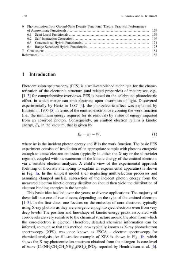
Photoemission spectroscopy (PES) is a well-established technique for the charac-

terization of the electronic structure (and related properties) of matter; see, e.g.,

[1–3] for comprehensive overviews. PES is based on the celebrated photoelectric

effect, in which matter can emit electrons upon absorption of light. Discovered

experimentally by Hertz in 1887 [4], the photoelectric effect was explained by

Einstein in 1905 [5] in terms of the emitted electron overcoming the work function

(i.e., the minimum energy required for its removal) by virtue of energy imparted

from an absorbed photon. Consequently, an emitted electron retains a kinetic

energy, Ek, in the vacuum, that is given by

Ek ¼ hv�W, ð1Þ

where hv is the incident photon energy and W is the work function. The basic PES

experiment consists of irradiation of an appropriate sample with photons energetic

enough to cause electron emission (typically in either the X-ray or the ultraviolet

regime), coupled with measurement of the kinetic energy of the emitted electrons

via a suitable electron analyzer. A child’s view of the experimental approach

(befitting of theorists attempting to explain an experimental apparatus) is shown

in Fig. 1a. In the simplest model (i.e., neglecting multi-electron processes and

assuming clamped nuclei), subtraction of the incident photon energy from the

measured electron kinetic energy distribution should then yield the distribution of

electron binding energies in the sample.

This basic idea has led, over the years, to diverse applications. The majority of

these fall into one of two classes, depending on the type of the emitted electrons

[1–3]. In the first class, one focuses on the emission of core-electrons, typically

using X-ray photons as they are energetic enough to eject electrons even from very

deep levels. The position and line-shape of kinetic energy peaks associated with

core-levels are very sensitive to the chemical structure around the atom from which

the core-electron is ejected. Therefore, detailed chemical information can be

inferred, so much so that this method, now typically known as X-ray photoelectron

spectroscopy (XPS), was once known as ESCA – electron spectroscopy for

chemical analysis. An illustrative example of XPS is shown in Fig. 1b, which

shows the X-ray photoemission spectrum obtained from the nitrogen 1s core level

of trans-[Co(NH2CH2CH2NH2)2(NO2)2]NO3, reported by Hendrickson et al. [6].

138 L. Kronik and S. Kummel

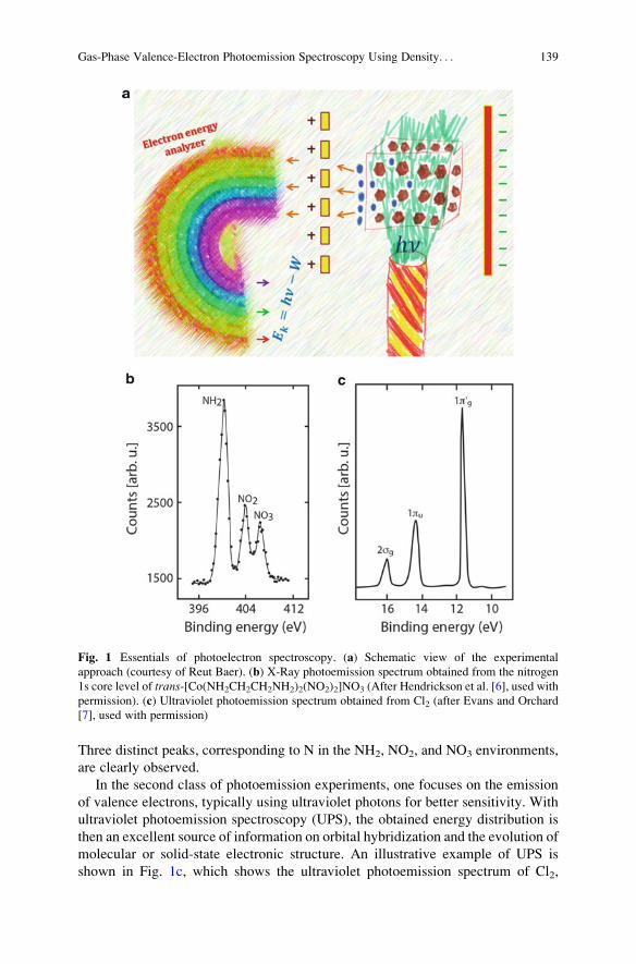
Three distinct peaks, corresponding to N in the NH2, NO2, and NO3 environments,

are clearly observed.

In the second class of photoemission experiments, one focuses on the emission

of valence electrons, typically using ultraviolet photons for better sensitivity. With

ultraviolet photoemission spectroscopy (UPS), the obtained energy distribution is

then an excellent source of information on orbital hybridization and the evolution of

molecular or solid-state electronic structure. An illustrative example of UPS is

shown in Fig. 1c, which shows the ultraviolet photoemission spectrum of Cl2,

Fig. 1 Essentials of photoelectron spectroscopy. (a) Schematic view of the experimental

approach (courtesy of Reut Baer). (b) X-Ray photoemission spectrum obtained from the nitrogen

1s core level of trans-[Co(NH2CH2CH2NH2)2(NO2)2]NO3 (After Hendrickson et al. [6], used with

permission). (c) Ultraviolet photoemission spectrum obtained from Cl2 (after Evans and Orchard

[7], used with permission)

Gas-Phase Valence-Electron Photoemission Spectroscopy Using Density. . . 139

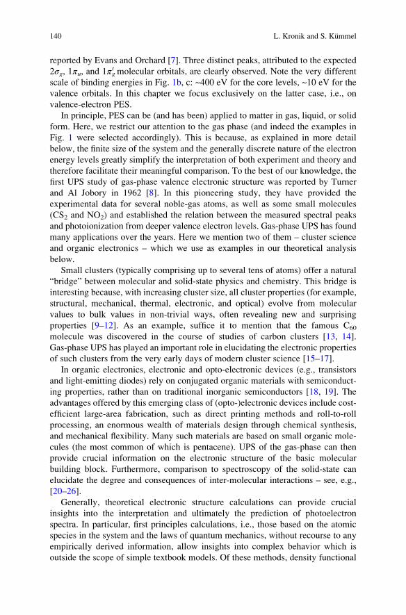
reported by Evans and Orchard [7]. Three distinct peaks, attributed to the expected

2σg, 1πu, and 1πg0 molecular orbitals, are clearly observed. Note the very different

scale of binding energies in Fig. 1b, c: ~400 eV for the core levels, ~10 eV for the

valence orbitals. In this chapter we focus exclusively on the latter case, i.e., on

valence-electron PES.

In principle, PES can be (and has been) applied to matter in gas, liquid, or solid

form. Here, we restrict our attention to the gas phase (and indeed the examples in

Fig. 1 were selected accordingly). This is because, as explained in more detail

below, the finite size of the system and the generally discrete nature of the electron

energy levels greatly simplify the interpretation of both experiment and theory and

therefore facilitate their meaningful comparison. To the best of our knowledge, the

first UPS study of gas-phase valence electronic structure was reported by Turner

and Al Jobory in 1962 [8]. In this pioneering study, they have provided the

experimental data for several noble-gas atoms, as well as some small molecules

(CS2 and NO2) and established the relation between the measured spectral peaks

and photoionization from deeper valence electron levels. Gas-phase UPS has found

many applications over the years. Here we mention two of them – cluster science

and organic electronics – which we use as examples in our theoretical analysis

below.

Small clusters (typically comprising up to several tens of atoms) offer a natural

“bridge” between molecular and solid-state physics and chemistry. This bridge is

interesting because, with increasing cluster size, all cluster properties (for example,

structural, mechanical, thermal, electronic, and optical) evolve from molecular

values to bulk values in non-trivial ways, often revealing new and surprising

properties [9–12]. As an example, suffice it to mention that the famous C60

molecule was discovered in the course of studies of carbon clusters [13, 14].

Gas-phase UPS has played an important role in elucidating the electronic properties

of such clusters from the very early days of modern cluster science [15–17].

In organic electronics, electronic and opto-electronic devices (e.g., transistors

and light-emitting diodes) rely on conjugated organic materials with semiconduct-

ing properties, rather than on traditional inorganic semiconductors [18, 19]. The

advantages offered by this emerging class of (opto-)electronic devices include cost-

efficient large-area fabrication, such as direct printing methods and roll-to-roll

processing, an enormous wealth of materials design through chemical synthesis,

and mechanical flexibility. Many such materials are based on small organic mole-

cules (the most common of which is pentacene). UPS of the gas-phase can then

provide crucial information on the electronic structure of the basic molecular

building block. Furthermore, comparison to spectroscopy of the solid-state can

elucidate the degree and consequences of inter-molecular interactions – see, e.g.,

[20–26].

Generally, theoretical electronic structure calculations can provide crucial

insights into the interpretation and ultimately the prediction of photoelectron

spectra. In particular, first principles calculations, i.e., those based on the atomic

species in the system and the laws of quantum mechanics, without recourse to any

empirically derived information, allow insights into complex behavior which is

outside the scope of simple textbook models. Of these methods, density functional


theory (DFT) [27–34] has become the method of choice for electronic-structure

calculations across an unusually wide variety of disciplines, from organic chemistry

[29] to condensed matter physics [35], as it allows for fully quantum-mechanical

calculations at a relatively modest computational cost. However, for reasons

discussed in greater detail below, the application of DFT to photoelectron spec-

troscopy has generated considerable controversy over the years, regarding both the

limitations of the theory in principle and its performance with popular approximate

forms in practice. In this chapter, we survey our recent progress in, and present

understanding of, this subtle issue. We emphasize both fundamental considerations

and practical applications, making appropriate links between the two.

The chapter is arranged as follows. We begin with the theory of the photoemis-

sion experiment from an elementary quantum mechanics point of view. Then we

explain how this view couples naturally to the more advanced many-body pertur-

bation theory view of photoemission. We then turn our attention to DFT. First, we

discuss a rigorous approach to photoemission within the framework of time-

dependent DFT (TDDFT). Then we focus on ground-state DFT. We clarify the

extent to which it can be used to mimic many-body perturbation theory in principle,

then provide a detailed discussion of the accuracy one can and cannot expect in

practice with various approximate DFT forms. We end with concluding remarks

and a brief outlook.

2 Photoemission from an Elementary Wave Function

Perspective

In the following, we start from the basic principles of quantum mechanics to relate

photoemission observables to the quantities that are typically accessible to elec-

tronic structure calculations. One of the basic assumptions that we make is that

perturbation theory, in the sense of Fermi’s golden rule, can be applied. In doing so,

we exclude non-perturbative photoemission processes. For our purposes this is not a

serious restriction because for elucidating the structure of the type of materials in

which we are most interested – semiconductors and organic molecules – experi-

ments are rarely done in the non-perturbative regime. We can therefore follow the

usual derivation [36, 37] and start from the observation that, according to Fermi’s

golden rule, the probability for a transition from an initial N-electron state |ΨNini to a

final state |ΨNf i that is triggered by a photon of energy ℏω of an electromagnetic

field with vector potential A is given by

Win!f / Ψ Nin

� ��A � P Ψ Nf

�� 2δ ℏωþ Ein � Efð Þ: ð2Þ

Here P is the momentum operator, and Ein and Ef are the initial and final state

energies, respectively. For clarity we assume that the N-electron molecule is

initially in its ground state ΨN0 with energy E0. In writing the final state one typically


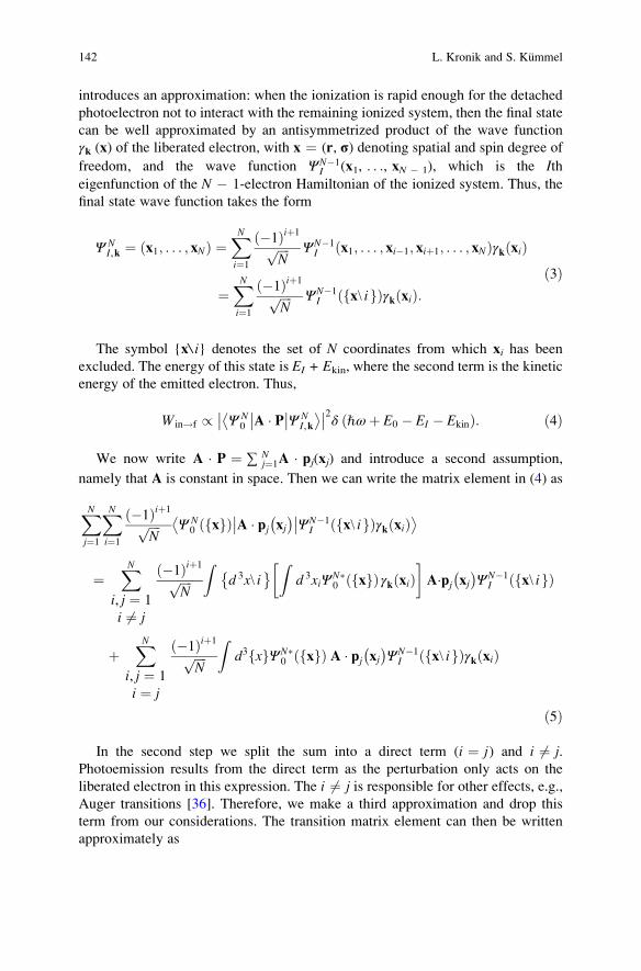
introduces an approximation: when the ionization is rapid enough for the detached

photoelectron not to interact with the remaining ionized system, then the final state

can be well approximated by an antisymmetrized product of the wave function

γk (x) of the liberated electron, with x ¼ (r, σ) denoting spatial and spin degree of

freedom, and the wave function ΨN�1I (x1, . . ., xN � 1), which is the Ith

eigenfunction of the N � 1-electron Hamiltonian of the ionized system. Thus, the

final state wave function takes the form

Ψ NI,k ¼ x1; . . . ; xNð Þ ¼

XNi¼1

�1ð Þiþ1ffiffiffiffiN

p ΨN�1I x1; . . . ; xi�1; xiþ1; . . . ; xNð Þγk xið Þ

¼XNi¼1


p ΨN�1I x\ if gð Þγk xið Þ:

ð3Þ

The symbol {x\ i} denotes the set of N coordinates from which xi has been

excluded. The energy of this state is EI + Ekin, where the second term is the kinetic

energy of the emitted electron. Thus,

Win!f / Ψ N0

� ��A � P Ψ NI,k

�� 2δ ℏωþ E0 � EI � Ekinð Þ: ð4Þ

We now write A � P ¼ ∑ Nj¼1A � pj(xj) and introduce a second assumption,

namely that A is constant in space. Then we can write the matrix element in (4) as

XNj¼1

XNi¼1


p Ψ N0 xf gð Þ� ��A � pj xj

� �ΨN�1

I x\ if gð Þγk xið Þ��

¼XN

i, j ¼ 1

i 6¼ j


pZ

d 3x\ i� Z

d 3xiΨN�0 xf gð Þγk xið Þ

�A�pj xj

� �ΨN�1

I x\ if gð Þ

þXN

i, j ¼ 1

i ¼ j


pZ

d3 xf gΨN�0 xf gð Þ A � pj xj

� �ΨN�1

I x\ if gð Þγk xið Þ

ð5Þ

In the second step we split the sum into a direct term (i ¼ j) and i 6¼ j.Photoemission results from the direct term as the perturbation only acts on the

liberated electron in this expression. The i 6¼ j is responsible for other effects, e.g.,Auger transitions [36]. Therefore, we make a third approximation and drop this

term from our considerations. The transition matrix element can then be written

approximately as


Ψ N0

� ��A � P Ψ NI,k

�� ¼ XNi¼1

�1ð Þiþ1

N

Zd3xi

ffiffiffiffiN

p Zd3x\ i

� ΨN�

0 xf gð ÞΨN�1I x\ if gð Þ

�|fflfflfflfflfflfflfflfflfflfflfflfflfflfflfflfflfflfflfflfflfflfflfflfflfflfflfflfflfflfflfflfflfflfflffl{zfflfflfflfflfflfflfflfflfflfflfflfflfflfflfflfflfflfflfflfflfflfflfflfflfflfflfflfflfflfflfflfflfflfflffl}

:¼ϕI xið Þ

�A � pi xið Þγk�xi�: ð6Þ

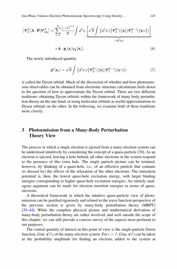
The newly introduced quantity

ϕI xið Þ ¼ffiffiffiffiN

p Zd3x\ i

� ΨN�

0 xf gð ÞΨN�1I x\ if gð Þ ð7Þ

is called the Dyson orbital. Much of the discussion of whether and how photoemis-

sion observables can be obtained from electronic structure calculations boils down

to the question of how to approximate the Dyson orbital. There are two different

traditions: obtaining Dyson orbitals within the framework of many body perturba-

tion theory on the one hand, or using molecular orbitals as useful approximations to

Dyson orbitals on the other. In the following, we examine both of these traditions

more closely.

3 Photoemission from a Many-Body Perturbation

Theory View

The process in which a single electron is ejected from a many-electron system can

be understood intuitively by considering the concept of a quasi-particle [38]. As an

electron is ejected, leaving a hole behind, all other electrons in the system respond

to the presence of this extra hole. The single particle picture can be retained,

however, by thinking of a quasi-hole, i.e., of an effective particle that contains

(is dressed by) the effects of the relaxation of the other electrons. The ionization

potential is, then, the lowest quasi-hole excitation energy, with larger binding

energies corresponding to higher quasi-hole excitation energies. An entirely anal-

ogous argument can be made for electron insertion energies in terms of quasi-

electrons.

A theoretical framework in which the intuitive quasi-particle view of photo-

emission can be justified rigorously and related to the wave function perspective of

the previous section is given by many-body perturbation theory (MBPT)

[39–44]. While the complete physical picture and mathematical derivation of

many-body perturbation theory are rather involved, and well outside the scope of

this chapter, we can still provide a concise survey of the aspects most pertinent to

our purposes.

The central quantity of interest in this point of view is the single-particle Green

function,G(xt, x0t0), of the many-electron system. For t > t0,G(xt, x0t0) can be takenas the probability amplitude for finding an electron, added to the system at


coordinates x0 and time t0, at coordinates x at a later time t. For t < t0, it correspondsto the probability amplitude for finding a missing electron, removed from the

system at coordinates x and time t, to be missing at coordinates x0 at a later time

t0. The two scenarios clearly correspond closely to the above concepts of the quasi-

electron and quasi-hole, respectively.

Many important properties can be extracted from the Green function (see, e.g.,

[45]). Among these, of chief interest here are those corresponding to the energy and

probability of electron insertion or removal. In the absence of external time-

dependent fields, one can assume time invariance, i.e., that the Green function

only depends on the relative time, t0 � t. A frequency-dependent Green function,

G(x,x0;ω), can then be defined using a Fourier transform. Importantly. this Green

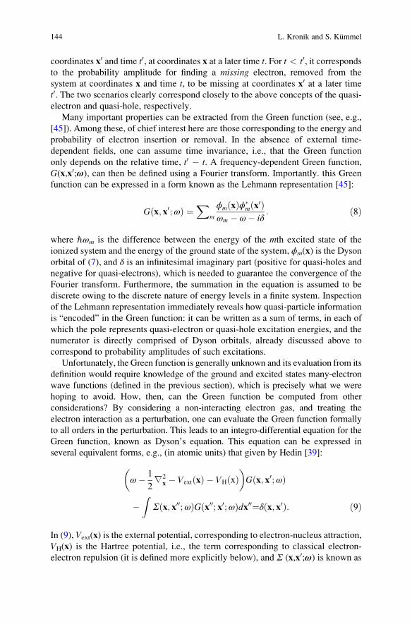
function can be expressed in a form known as the Lehmann representation [45]:

G x; x0;ωð Þ ¼X

m

ϕm xð Þϕ�m x0ð Þ

ωm � ω� iδ: ð8Þ

where ℏωm is the difference between the energy of the mth excited state of the

ionized system and the energy of the ground state of the system, ϕm(x) is the Dyson

orbital of (7), and δ is an infinitesimal imaginary part (positive for quasi-holes and

negative for quasi-electrons), which is needed to guarantee the convergence of the

Fourier transform. Furthermore, the summation in the equation is assumed to be

discrete owing to the discrete nature of energy levels in a finite system. Inspection

of the Lehmann representation immediately reveals how quasi-particle information

is “encoded” in the Green function: it can be written as a sum of terms, in each of

which the pole represents quasi-electron or quasi-hole excitation energies, and the

numerator is directly comprised of Dyson orbitals, already discussed above to

correspond to probability amplitudes of such excitations.

Unfortunately, the Green function is generally unknown and its evaluation from its

definition would require knowledge of the ground and excited states many-electron

wave functions (defined in the previous section), which is precisely what we were

hoping to avoid. How, then, can the Green function be computed from other

considerations? By considering a non-interacting electron gas, and treating the

electron interaction as a perturbation, one can evaluate the Green function formally

to all orders in the perturbation. This leads to an integro-differential equation for the

Green function, known as Dyson’s equation. This equation can be expressed in

several equivalent forms, e.g., (in atomic units) that given by Hedin [39]:

ω� 1

2∇2

x � Vext xð Þ � VH xð Þ �

G x; x0;ωð Þ

�Z

Σ x; x00;ωð ÞG x00; x0;ωð Þdx00¼δ x; x0ð Þ: ð9Þ

In (9), Vext(x) is the external potential, corresponding to electron-nucleus attraction,

VH(x) is the Hartree potential, i.e., the term corresponding to classical electron-

electron repulsion (it is defined more explicitly below), and Σ (x,x0;ω) is known as


the self-energy – it is the precise mathematical expression of the above-mentioned

“dressing” of the electron by its environment, beyond the simple electrostatic

picture of the Hartree potential.

Using the Lehmann representation of (8) in (9) leads to the Schwinger form of

Dyson’s equation, given (in atomic units) by

� 1

2∇2 þ Vext xð Þ þ VH xð Þ

�ϕm xð Þ

þZ

Σ x; x0; εmð Þϕm x0ð Þdx0¼ωmϕm xð Þ: ð10Þ

Equation (10) resembles the time-independent single-particle Schrodinger equa-

tion. As with the Schrodinger equation itself, its eigenvalues correspond to energies

and its eigenfunctions are related to probability amplitudes (naturally, for the

extraction of probabilities the eigenfunctions need to be normalized so as to

conform to (7)). However, there are key differences. First, while Dyson’s equation

has the form of a single-particle equation, it is in fact an exact many-particle

equation, with many-electron information contained in the self-energy operator.

Second, Dyson’s equation does not predict steady-state energies, but rather charged

excitation energies. Last, but by no means least, whereas the potential in

Schrodinger’s equation is a multiplicative operator, the self-energy is in general

non-multiplicative, frequency-dependent, and even non-Hermitian (reflecting, e.g.,

finite lifetime effects).

While Dyson’s equation provides an interesting and rigorous framework for the

quasi-particle point of view, in the absence of further information it is still insuf-

ficient as a basis for practical computation. This is because generally the self-

energy, Σ(x,x0;ω), is as unknown as the Green function, G(x,x0;ω). Hedin [39]

has suggested that a practical way forward can be obtained by considering an

expansion of the self-energy operator in terms of the dynamically screened Cou-

lomb interaction,W(x,x0;ω), which is related to the bare Coulomb repulsion via the

inverse dielectric matrix, ε�1 (x, x0;ω). This leads to a set of five coupled integral

equations, from which both Σ(x,x0;ω) and G(x,x0;ω) can formally be extracted.

Practically, the hope is that because the screened Coulomb potential, W(x, x0;ω), isweaker than the bare one, the self-energy expansion would converge rapidly and

that, ideally, only its leading term would need to be retained. This leads to a

relatively simple expression of the self-energy in terms of G and W:

Σ x; x0;ωð Þ ¼ i

2π

Zdω0eiδω

0G x; x0;ω0ð ÞW x, x0;ω� ω0ð Þ, ð11Þ

where δ is an infinitesimal convergence factor. Equation (11) is known as the GWapproximation.

For (11) to be used in conjunction with (10) as a practical tool, one still needs to

know how to calculate G and W. Typically, one first performs a ground-state DFT


calculation, explained in the next section, then computes G and W (and ergo Σ)based on the DFT orbitals and solves Dyson’s equation. This simplified procedure

is sometimes known as a “one-shot” GW calculation or as a G0W0 calculation.

Despite the seeming crudeness of the procedure, it often provides surprisingly

accurate excitation energies, even in molecular systems where screening is usually

not nearly as strong as in solids. As one representative and early example of the

application of GW to molecules, consider that for silane (SiH4) the ionization

potential obtained as the lowest quasi-hole excitation energy from Dyson’s equa-

tion in the G0W0 approximation is 12.7 eV [46], as compared to an experimental

value of 12.6 eV. A similar degree of agreement between G0W0 and experiment

and/or wave function-based theory has also been found for other small molecules,

e.g., CO and BeO [47, 48]. We note, however, that agreement is not always this

good, notably for the electron affinity – see, e.g., [49–51]. Also, the results of

differentGW calculations can differ considerably, as also exemplified by the case of

Silane [52–55]. The pros and cons of refining the GW method via partial or full

iteration to self-consistency and/or modified choices of the DFT starting point, as

well as the limitations of theGW approximation itself in any form, constitute a topic

of active and lively debate. This discussion is far too varied and contemporary to

survey in any meaningful detail here. We do note, however, that this means that the

“umbrella term” GW is insufficient to define uniquely a given computation, which

may vary in DFT starting point, iterative approach (or lack thereof), and many

additional details and approximations in the evaluation of both G and W.

4 Photoemission from a Rigorous Density Functional

Theory View: Excited-State Theory

4.1 Concepts of Ground-State Density Functional Theory

DFT [27–34] is an approach to the many-electron problem in which the electron

density, rather than the many-electron wave function, plays the central role. As

already mentioned in the introduction, DFT is by far the most common first

principles electronic structure theory, as it allows for fully quantum-mechanical

calculations at a relatively modest computational cost. It is therefore of great

interest to assess how the theory of photoemission, which we have already exam-

ined from the many-body wave function and the many-body perturbation theory

points of view, can be rigorously captured within DFT.

Just as with MBPT, the complete physical picture and mathematical derivation

of DFT are rather involved and are well outside the scope of this chapter. Never-

theless, here too we can still provide a concise survey of the aspects most pertinent

to our purposes. The central tenet of DFT is the Hohenberg–Kohn theorem [56],

which states that the ground-state density, n(r), of a system of interacting electrons

subject to some external potential, vext(r), determines this potential uniquely (up to


a physically trivial constant). The importance of this theorem lies in the fact that

(within the Born–Oppenheimer approximation) any system is completely described

by the number of electrons in it, which is simply an integral of n(r) over space, andby the types and positions of the nuclei in it. However, the effect of the latter two

quantities on the electron system is given completely by the ion–electron attraction

potential. This potential is external to the electron system and therefore, according

to the Hohenberg–Kohn theorem, is uniquely determined by the ground-state

density. This means that the ground-state density contains all the information

needed to describe the system completely and uniquely.

The above considerations are typically not employed directly, but rather are used

in the construction of the Kohn–Sham (KS) equation [57], which is the “workhorse”

of DFT. In Kohn–Sham DFT, the original interacting-electron Schrodinger equa-

tion is mapped into an equivalent problem of fictitious, non-interacting electrons,

such that the ground-state density of the non-interacting system is equal to that of

the original system. This leads to a set of effective one-particle equations, which in

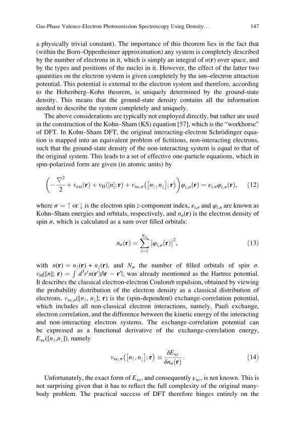
spin-polarized form are given (in atomic units) by

�∇2

2þ vext rð Þ þ vH n½ �; rð Þ þ vxc,σ n"; n#

� �; r

� � �φi,σ rð Þ ¼ εi,σφi,σ rð Þ, ð12Þ

where σ ¼ " or # is the electron spin z-component index, εi,σ and φi,σ are known as

Kohn–Sham energies and orbitals, respectively, and nσ(r) is the electron density of

spin σ, which is calculated as a sum over filled orbitals:

nσ rð Þ ¼XNσ

i¼1

φi,σ rð Þ�� 2, ð13Þ

with n(r) ¼ n"(r) + n#(r), and Nσ the number of filled orbitals of spin σ.vH([n]; r) ¼

Rd3r0n(r0)/|r � r0|, was already mentioned as the Hartree potential.

It describes the classical electron-electron Coulomb repulsion, obtained by viewing

the probability distribution of the electron density as a classical distribution of

electrons. vxc,σ([n", n#]; r) is the (spin-dependent) exchange-correlation potential,

which includes all non-classical electron interactions, namely, Pauli exchange,

electron correlation, and the difference between the kinetic energy of the interacting

and non-interacting electron systems. The exchange-correlation potential can

be expressed as a functional derivative of the exchange-correlation energy,

Exc([n",n#]), namely

vxc,σ n"; n#� �

; r� � � δExc

δnσ rð Þ : ð14Þ

Unfortunately, the exact form of Exc, and consequently νxc, is not known. This isnot surprising given that it has to reflect the full complexity of the original many-

body problem. The practical success of DFT therefore hinges entirely on the


existence of suitable approximations for Exc. The earliest, appealingly simple

approximation for the exchange-correlation energy functional, already suggested

by Kohn and Sham [57], is the local density approximation (LDA) or, in its

spin-polarized form, the local spin density approximation (LSDA) [58, 59].

In this approximation, we assume that at each point in space the exchange-

correlation energy per particle is given by its value for a homogeneous electron

gas, exc(n"(r), n#(r)), namely

ELSDAxc n"; n#

� � ¼ Zd3rn rð Þexc n" rð Þ, n# rð Þ� �

: ð15Þ

The L(S)DA has several advantages. First, exc(n"(r), n#(r)) is unique because ofthe theoretical existence of a system with uniform spin densities. Second, there is

ample information on exc: it was already known approximately when Hohenberg,

Kohn, and Sham were formulating DFT, and has since been computed more

accurately using Monte Carlo methods [60]. Furthermore, several useful analytical

parametrizations of the Monte Carlo results, that also take into account other known

limits and/or scaling laws of exc, have been given [61–63]. Last, but not least, the

exchange-correlation potential, given by (14), becomes a simple function, ratherthan a functional, of n"(r) and n#(r). The difficulty with L(S)DA is that in real

systems the density is clearly not uniform. More often than not, it actually exhibits

rapid changes in space. L(S)DA was therefore expected to be of limited value in

providing an accurate description of the electron interaction [57]. Nevertheless, it

has often been found to provide surprisingly accurate predictions of experimental

results (see, e.g., [64]), partly due to a systematic cancellation of errors between the

exchange and correlation terms. More advanced approximate functionals, designed

to overcome these limitations partly, are discussed in detail in Sect. 6. However,

L(S)DA is sufficient to establish that DFT can indeed be a practical tool and not just

a formal framework.

The degree to which single-electron DFT quantities can approximate quasi-

particle quantities is discussed in detail in Sect. 5. However, in any case, DFT is

a ground-state theory, while we are obviously trying to obtain quantities manifestly

related to excitation. Rigor can therefore be restored by considering TDDFT

[65–68] – a generalization of the original theory that is suitable for studies of

excited states.

4.2 Time-Dependent Density Functional Theoryand Photoemission

Just as DFT rests on the Hohenberg–Kohn theorem, TDDFT rests on the Runge–

Gross theorem [69], which establishes a one-to-one correspondence between the

time-dependent density and a time-dependent external potential. When the


interaction of an electronic system with light is modeled by a classical electric field

that is described by a time-dependent external scalar potential, the corresponding

electron dynamics can be obtained from the time-dependent Kohn–Sham equations

(in atomic units):

�∇2

2þ vext r; tð Þ þ vH n½ �; r; tð Þ þ vxc,σ n"; n#

� �; r; t

� �0@

1Aφi,σ r; tð Þ

¼ i∂∂t

φi,σ r; tð Þ,ð16Þ

i.e., the time-dependent analogue of (12). The time-dependent density follows from

(13) with the time-dependent orbitals replacing the static ones. In (16) the Hartree

and exchange-correlation potential inherit a time-dependence from the time-

dependence of the density.

In principle these equations allow for a parameter free, first principles calcula-

tion of photoemission, because the photoemission information is encoded in the

time-dependent density. The latter can, in principle, be obtained exactly from (16).

However, in practice the situation is more complicated, with complications arising

at different levels. First, the exact time-dependent exchange-correlation potential is

not known and approximations for it must be used. These approximations may need

to be rather involved functionals of the density, because not only does the time-

dependent vxc,σ share some of the intricacies of the ground-state exchange-correla-

tion potential (such as the derivative discontinuity [70] discussed in detail in

Sect. 5) but also it offers additional challenges that are not present in ground-state

DFT. Prominent examples are the initial-state and memory effects [71], i.e., the

dependence of the exchange-correlation functional on the initial conditions and on

the history of the density and not just its present form.

Even when sufficiently accurate approximations for vxc,σ are known, it is not

obvious how photoemission observables are to be calculated, because rigorously

speaking the orbitals in (16) only serve to build the density. The physical meaning

of these orbitals is discussed at length in Sect. 5, but in a traditional view that

focuses only on exact relations, they are not endowed with a precise physical

interpretation. Consequently, all observables should be calculated from the density.

The exact, explicit density functional for the photoemission intensity is, however,

so far unknown. Therefore, approximations must also be used at the level of

calculating the observables. Different ways in which TDDFT allows the extraction

of information about photoemission in practice, by making such approximations,

are discussed in the following.

A first approach to extract photoemission information from a TDDFT calcula-

tion builds on the fact that the photoemission energies, i.e., the peaks in the

recorded photoemission signal, are directly related to the eigenenergies EI of the

N � 1 electron system that remains after detection of the photoelectron, cf. (4). If

the ultimate vxc,σ were known, the N � 1-electron system’s ground state and


excited state energies could be calculated exactly, e.g., by transforming to the

frequency domain and using TDDFT in the linear-response limit [36, 72] or by

analyzing [73] the density response obtained from real-time propagation solution

[74] of (16). For many systems the commonly available approximations for vxc,σ areaccurate enough to yield excitation energies of finite systems with reasonable

accuracy. Therefore, the energetic positions at which photoemission peaks can

occur are accessible even in practice [36, 73, 75]. The problem that remains,

though, is to know with which intensity a photoemission signal will be detected

at each of the possible energies.

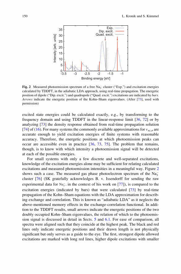
For small systems with only a few discrete and well-separated excitations,

knowledge of the excitation energies alone may be sufficient for relating calculated

excitations and measured photoemission intensities in a meaningful way. Figure 2

shows such a case. The measured gas phase photoelectron spectrum of the Na�3cluster [76] (SK gratefully acknowledges B. v. Issendorff for sending the raw

experimental data for Na−3 , in the context of his work on [77]), is compared to the

excitation energies (indicated by bars) that were calculated [73] by real-time

propagation of the Kohn–Sham equations with the LDA approximation for describ-

ing exchange and correlation. This is known as “adiabatic LDA” as it neglects the

above-mentioned memory effects in the exchange-correlation functional. In addi-

tion to the TDDFT results, small arrows indicate the energetic positions of the two

doubly occupied Kohn–Sham eigenvalues, the relation of which to the photoemis-

sion signal is discussed in detail in Sects. 5 and 6.1. For ease of comparison, all

spectra were aligned such that they coincide at the highest peak. The black and red

lines only indicate energetic positions and their drawn length is not physically

significant but only serves as a guide to the eye. The first, strongest dipole allowed

excitations are marked with long red lines, higher dipole excitations with smaller

0

5

10

15

20

25

30

35

-3.5 -3 -2.5 -2 -1.5 -1

Inte

nsity

[arb

. uni

ts]

Binding energy [eV]

Exp.Dip. excit.

Quad. excit.

Fig. 2 Measured photoemission spectrum of a free Na�3 cluster (“Exp.”) and excitation energies

calculated by TDDFT, in the adiabatic LDA approach, using real-time propagation. The energetic

position of dipole (“Dip. excit.”) and quadrupole (“Quad. excit.”) excitations are indicated by bars.Arrows indicate the energetic position of the Kohn–Sham eigenvalues. (After [73], used with

permission)


red lines, and quadrupole excitations correspondingly with black dotted lines. The

figure shows that there are electronic transitions corresponding to each peak in the

spectrum, and that the TDDFT approach allows one to obtain information about

the photoemission intensities at binding energies below �2 eV, which cannot be

explained based on the eigenvalue approach discussed below (note that for spin-

unpolarized calculations of Na�3 , as here, there are only two eigenvalues

corresponding to valence electrons). However, for this simple system it is already

apparent that access to only the energetic positions, without being able to predict

intensities (i.e., peak heights), is a limitation.

This limitation becomes very serious when the system of interest shows a wealth

of excitations and the majority of them are not visible in the photoemission

experiment. Knowing with which intensity an excitation contributes to the photo-

emission signal then is mandatory for a meaningful interpretation of the data. The

situation can be seen in analogy to a photoabsorption calculation. Without knowing

the oscillator strength that is associated with a transition, the photoabsorption

spectrum cannot be predicted, because one needs the oscillator strength to distin-

guish between forbidden and allowed transitions. However, there is a decisive

difference between the TDDFT calculation of photoabsorption and photoemission.

Photoabsorption intensities are related to oscillator strengths, and the latter can be

calculated from the frequency dependent dipole moment. The dipole moment is

itself an explicit functional of the density and thus very naturally accessible in

TDDFT. The intensity of the photoemission peaks, on the other hand, is related to

the matrix element that appears in (4). This matrix element cannot – to the best of

our knowledge – be simplified to yield an expression that explicitly depends on the

density. Evaluating it would require knowledge of the wavefunction – but the latter

is not known in (TD)DFT. Therefore, whereas excitation energies can rigorously be

calculated from TDDFT, the photoemission intensities cannot.

In order to make further progress one has to invoke additional approximations.

One possibility is to approximate the true correlated wavefunction ΨN�1I of Sect. 2

by the Ith Slater-determinant of Kohn–Sham orbitals. It has been argued [78–81]

that, among all non-interacting wave-functions, the Kohn–Sham Slater-determinant

is likely to approximate the true wave-function best because it is density optimal.

However, it is also well known that there are systems for which any single Slater-

determinant is not a good approximation to the true wavefunction. Luckily, for

organic systems the single Slater-determinant approximation can often be justified.

When this is the case, (4) can be evaluated with ΨN�1I replaced by either the Slater-

determinant ΨKS,0 calculated from a self-consistent ground-state calculation for the

N � 1 electron system to obtain the first emission peak or, for further peaks, with

the Ith excited-state Kohn–Sham Slater-determinant. The latter can be obtained

from the linear-response TDDFT (for the N � 1 electron system), given (in the

Tamm–Dancoff approximation) in the form [72]


ΨKS, I ¼Xiocc:

Xj unocc:

kij, Ic{j ciΨKS,0: ð17Þ

Here, c{j and ci are creation and annihilation operators referring to the Kohn–Sham

single particle basis, kij,I are the weights with which the i, j particle-hole transitioncontributes to the Ith excitation, and the sums run over all occupied or unoccupied

orbitals, respectively. Using this equation, the Dyson orbital of (7) can also be

approximately expressed as an overlap of Kohn–Sham Slater-determinants [37, 82].

The approach just described – calculating excitation energies within the rigorous

framework of TDDFT, but for the transition strengths making the possibly far

reaching approximation of using the Kohn–Sham Slater-determinant in place of

the true wavefunction – is not the only way of extracting photoemission observables

from TDDFT calculations. Instead of trying to tie in with the concepts of Sect. 2 and

focusing on the N � 1-electron system and its wavefunction, one can instead make

the transition from traditional wavefunction-based quantum mechanics to TDDFT

at an earlier stage and focus directly on the TDDFT simulation of the photoemission

process. Thus, instead of the N � 1-electron system, one directly simulates the N-electron system. With the help of (12) and (16) the corresponding computational

procedure is straightforward. First calculate the ground-state of the N-electronsystem by solving the time-independent Kohn–Sham equations, then switch on

the classical electric field in the form of an explicitly time-dependent, oscillating

linear (dipole) potential and let the system evolve according to the time-dependent

Kohn–Sham equations. If the vxc,σ-approximation employed is accurate enough and

the numerical representation allows for the density escaping towards large distances

of the system’s center, e.g., by using large real-space grids, then the resulting

electron dynamics will faithfully reproduce the photoemission process in terms of

the time-dependent density.

Focusing in this way on the N- instead of the N � 1-electron system has

advantages. For example, there is no need for assumptions about the nature of the

state of the emitted electron, γk, that was introduced in Sect. 2, and nuclear

dynamics can straightforwardly be included at the Ehrenfest level. Also, as the

Kohn–Sham equations are directly solved numerically, the approach is not limited

to the linear response regime, but can also be used for simulating non-perturbative

photoemission, e.g., as triggered by highly intense lasers. This type of approach has

therefore frequently been employed for calculating approximate average ionization

probabilities, e.g., in [83–85]. By dividing space into a region close to the system in

which electrons are considered bound and a region far away from the system in

which electrons are considered unbound, the average ionization can be obtained by

integrating the total (or orbital) density over the bound region.

For calculating the kinetic energy spectrum of the photoemitted electrons, a

calculation based on (16) faces the problem of extracting the photoemission observ-

ables from the time-dependent density. In other words, a problem similar to the one

described above for the N � 1-electron TDDFT approach emerges. One solution to


this problem that has been suggested in the past is to use real-space grids [86, 87]

and record the time-dependent orbitals φi,σ(rO,t) at one or several observation

point(s), rO, far from the system. Then Fourier-transform the orbitals with respect

to t in order to find φiσ(rO,ω), and calculate the intensity of electrons emitted with a

kinetic energy Ekin from the equation

I rO;Ekinð Þ ¼Xσ¼", #

XNσ

j¼1

��φjσ rO,ω ¼ Ekin=ℏð Þ��2: ð18Þ

This procedure can be rationalized by thinking about the orbital at the recording point as a

plane wave expansion, φjσ (rO,t) ¼ Σω ec jσ,ω exp[i (k�rO � ωt)] ¼ Σω cjσ,ω exp(�iωt).The sum over the squares of the absolute values of the orbitals’ (at point rO)

Fourier-transforms (with respect to t) reflects the total probability amplitudeXσ¼",#

XNσ

j¼1cjσ,ω�� 2, with which a plane wave of energy ℏω is detected at the

observation point.

Equation (18) avoids the association of a specific orbital with a specific emission

energy. It is thus more general than the interpretation relying on orbital eigenvalues

that is discussed in detail in the next section. In addition, the approach very

naturally allows for extracting directional information about the photoemission

process: recording the orbitals at different observation points (which can be done

within one calculation) allows one to calculate angularly resolved photoemission

intensities in a very natural way. However, one has to note that this approach is not

an exact one – it still relies on a direct interpretation of the orbitals. More formally

phrased, (18) constitutes an implicit density functional for the photoemission

intensity, but an approximate one.

Beyond the formal limitation, much more serious difficulties for the practical use

of (18) result from seemingly “simple” technical issues. Allowing the density to

escape to regions of space that are far away from the system’s center precludes the

use of small, atom-centered basis sets that computationally can be handled very

efficiently. Instead, real space grids are employed to allow for an unbiased and

accurate representation of the density in all regions of space. Real-time, real-space

propagation calculations on grids as large as those required for an accurate deter-

mination of the photoemission signal are, however, computationally very time

consuming. In addition, one has to ensure that the outgoing density is not reflected

at the boundaries of the numerical simulation grid. This can in principle be achieved

with complex absorbing potentials [88] or mask functions [89, 90]. In practice,

however, it turns out that adjusting the absorbing layer such that the photoemission

signal can be recorded without substantial numerical noise, without an unphysical

dependence on the chosen observation point, and without disturbances due to the

boundary layer, is a tedious task. The adjustment has to be done anew for each

system and set of laser parameters [90, 91]. Therefore, the technique is not easy to

use for large systems with a complex electronic structure.

As an alternative to the observation point method, one can invoke the concept of

the Wigner transform for calculating the momentum distribution of the


photoemitted electrons. The Wigner transform of the one-body density matrix can

be interpreted as a semi-classical, approximate probability distribution for finding a

particle with a certain momentum at a certain position. The concept has been used

in calculations with correlated wavefunctions [92] and it has been transferred to

TDDFT by using the Kohn–Sham one-body density matrix

ρKS r, r0, tð Þ ¼Xj, occ

φ�j r; tð Þφj r

0, tð Þ ð19Þ

instead of the interacting one-body density matrix. In addition to the Wigner

function, which is not free of ambiguities itself, this involves the further assumption

that the interacting one-body density matrix far from the system’s center should be

well represented by (19). This is again an approximation, the accuracy of which is

hard to predict. However, calculations for small molecules indicate that the concept

is quite useful in practice. For details on the Wigner function approach we refer the

reader to [90].

In summary, TDDFT allows the calculation of excitation energies in a way that

is formally correct and exact in principle. Yet, as the density functional for the

photoemission intensities is not known, approximations have to be invoked for

calculating observables such as the intensities. The techniques described in this

section have so far almost exclusively been used for relatively small systems. This

is understandable, as TDDFT calculations are computationally much more inten-

sive than DFT calculations. Therefore, it is highly desirable to look for less

demanding ways of extracting photoemission information from electronic structure

calculations, preferably requiring only ground-state quantities. To which extent and

how this can be achieved is the topic of the next section.

5 Photoemission from an Approximate Density Functional

Theory View: Ground-State Theory

While TDDFT can provide a rigorous theoretical approach to photoemission, in

light of its above-mentioned difficulties it is still clearly tempting to utilize the

conceptually and computationally simpler ground-state DFT. This would be possi-

ble if we could identify the Kohn–Sham energies and orbitals, εi and φi of (12), with

the quasi-particle energies and Dyson orbitals, ℏωi and ϕi, respectively, of (10).

This identification may naively appear to be obvious, as both cases involve single-

electron energies and orbitals. Furthermore, it is relatively straightforward to show

that, for a non-interacting electron gas, insertion of the single-electron energies and

orbitals in the Lehmann representation of (8) yields the non-interacting Green

function [45]. This means that εi, and φi really are the quasi-particle energies and

Dyson orbitals of the non-interacting Kohn–Sham electron gas.


However, do εi, and φi correspond to the same quantities in the original,

interacting electron system? As explained above, the Kohn–Sham electron gas is

a fictitious system of non-interacting electrons in their ground state, obtained based

on a unique mapping from the physical system of electrons in their ground state.

The criterion leading to the KS mapping is that both systems have the same ground

state density. Therefore, any physical property of the real and fictitious system

which is determined directly and solely by the electron density (e.g., the electronic

dipole moment) must be the same for both systems. However, any other property

(e.g., the total energy, the kinetic energy, the current density, etc.) are not neces-

sarily identical between the two systems. This means that εi and φi need not

necessarily correspond to ℏωi and ϕi of the original system. Strictly speaking, εi,φi are merely auxiliary devices en route to the ground state density. In fact there is

nothing in the original proof of the KS construct [57] to suggest that KS single-

electron quantities carry the physical meaning of corresponding many-body per-

turbation theory quasi-particle quantities (or, for that matter, any meaning at all).

What relations, if any, do exist then between Kohn–Sham quantities and quasi-

particle properties? It is well known that the ground state density, n(r), of a finite,bound system of electrons (whether interacting or not), decays exponentially as

r ! 1, with a decay constant given (in atomic units) by 2ffiffiffiffiffi2I

p, where I is the

fundamental ionization energy (i.e., negative of the lowest quasi-hole energy)

[93, 94]. Because the physical and Kohn–Sham systems share the same density,

they must possess identical ionization potentials. Hence, the energy of highest

occupied molecular orbital (HOMO) of the Kohn–Sham system, εH, already

established to correspond to �I of the fictitious system, automatically also corre-

sponds to �I of the real system. We therefore obtain an important relation, known

as the ionization potential theorem [93–96] or as “the equivalent of Koopmans’

theorem in DFT”:

�εH ¼ I ð20Þ

Note that the original Koopmans’ theorem [97] states a relation identical to (20)

as an approximate result, which neglects orbital relaxation upon electron ejection,

within Hartree–Fock theory, which itself neglects correlation. The DFT version of

this theorem is in fact stronger – it is an exact relation, not an approximate one.

Because of (20), the Kohn–Sham HOMO eigenvalue should indeed, satisfyingly,

correspond to the leading photoemission peak.

Encouraged by this success, we can ask whether the same conclusion can be

reached for the other occupied Kohn–Sham states. Here, unfortunately, there is no

such rigorous justification. In fact, in general such an identification cannot be exact

[98]. While being profoundly different physically, mathematically the Kohn–Sham

equation (12) differs from the Dyson equation (10) only in that the self-energy is

replaced by the exchange-correlation potential. However, whereas the former

operator is non-multiplicative, frequency-dependent, and non-Hermitian, the latter

operator is multiplicative, frequency-independent, and Hermitian. Sham and

Schluter derived an exact relation between the self-energy operator and the


Kohn–Sham exchange-correlation potential, by constructing an integral equation

that connects these quantities and the Green function [99]. Using this relation, the

Kohn–Sham exchange-correlation potential can be interpreted as the variationally

best local approximation to the self-energy expression [100]. This gives us hope

that the solutions of the Dyson and Kohn–Sham equations need not be completely

unrelated. Nevertheless, there is no reason to think that the two equations would

yield the same eigenvalues throughout.

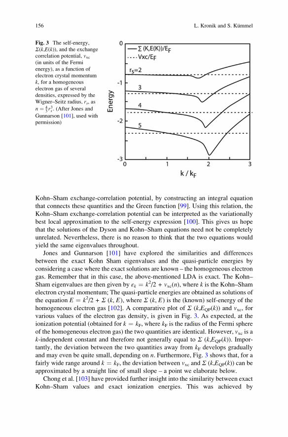
Jones and Gunnarson [101] have explored the similarities and differences

between the exact Kohn Sham eigenvalues and the quasi-particle energies by

considering a case where the exact solutions are known – the homogeneous electron

gas. Remember that in this case, the above-mentioned LDA is exact. The Kohn–

Sham eigenvalues are then given by εk ¼ k2/2 + vxc(n), where k is the Kohn–Shamelectron crystal momentum; The quasi-particle energies are obtained as solutions of

the equation E ¼ k2/2 + Σ (k, E), where Σ (k, E) is the (known) self-energy of the

homogeneous electron gas [102]. A comparative plot of Σ (k,EQP(k)) and vxc, forvarious values of the electron gas density, is given in Fig. 3. As expected, at the

ionization potential (obtained for k ¼ kF, where kF is the radius of the Fermi sphere

of the homogeneous electron gas) the two quantities are identical. However, vxc is ak-independent constant and therefore not generally equal to Σ (k,EQP(k)). Impor-

tantly, the deviation between the two quantities away from kF develops gradually

and may even be quite small, depending on n. Furthermore, Fig. 3 shows that, for a

fairly wide range around k ¼ kF, the deviation between vxc and Σ (k,EQP(k)) can beapproximated by a straight line of small slope – a point we elaborate below.

Chong et al. [103] have provided further insight into the similarity between exact

Kohn–Sham values and exact ionization energies. This was achieved by

Fig. 3 The self-energy,

Σ(k,E(k)), and the exchange

correlation potential, vxc(in units of the Fermi

energy), as a function of

electron crystal momentum

k, for a homogeneous

electron gas of several

densities, expressed by the

Wigner–Seitz radius, rs, as

n ¼ 43r3s . (After Jones and

Gunnarson [101], used with

permission)


reconstructing the exact Kohn–Sham potential from the exact density for several

atomic and small molecular systems and comparing the obtained eigenvalues to

experimental photoemission energies. Their results agreed very well with the above

findings for the homogeneous electron gas. They found that for eigenvalues close to

εH (often called outer valence orbital energies), the correspondence between Kohn–

Sham theory and experiment was very close, with deviations typically on the order

of 0.05–0.1 eV. This deviation is at least a factor of ten better than the typical

deviation with a Hartree–Fock calculation, and often close to the experimental

resolution. In agreement with the above-mentioned findings of Jones and

Gunnarson, for deeper levels Chong et al. found that the Kohn–Sham eigenvalues

exhibited increasingly larger deviations, ultimately reaching an order of 10 eV

(which is similar to the errors made by Hartree–Fock theory). Chong et al. further

established that – εi is the leading contribution to the ith quasi-particle energy, withadditional contributions determined by the overlaps between the densities of the KS

orbitals, as well as by overlaps between the KS and Dyson orbital densities.

Because photoemission involves the removal of electrons, up to this point we

have been comparing quasi-hole energies to occupied KS orbital energies. One can

also ask a closely related question on the similarities and differences between quasi-

electron energies and the energies of unoccupied Kohn–Sham orbitals. This ques-

tion is directly relevant when trying to interpret inverse photoemission spectros-

copy (IPES), where photons are emitted from a sample due to its irradiation with

fixed-energy electrons and the energy distribution of the emitted photons is mea-

sured [1]. Because we are unaware of any applications of IPES in the gas phase, we

do not dwell on it in this chapter. However, Fig. 3 indicates that the considerations

we have made for the similarities and differences between Kohn–Sham occupied

orbital energies and quasi-hole energies should also apply to unoccupied (virtual)

Kohn–Sham orbital energies and quasi-electron energies. However, the homoge-

neous electron gas of Fig. 3 is metallic. For a non-metallic system, one should still

ask whether there is a relation equivalent to (20) between the electron affinity, A,and the energy of the lowest unoccupied molecular orbital (LUMO) of the Kohn–

Sham system, εL. Equivalently, one should ask whether one can equate the funda-

mental quasi-particle gap, Eg ¼ I � A, and the KS gap, EKSg ¼ εL � εH.

Unfortunately, even with the exact KS potential, the answer is no [99, 104]. This

is due to a peculiar property of the exact Kohn–Sham potential – the derivative

discontinuity (DD) [95]. Briefly, for any system with a non-zero fundamental gap,

the derivative of the total energy with respect to particle number must be discon-

tinuous at the N-electron point. This is simply a reflection of the discontinuity in the

chemical potential, i.e., the fact that the electron removal energy is not the same as

the electron insertion energy. Consider how this is reflected in the KS description of

the total energy. Because the energy contributions of the external potential and the

Hartree potential are continuous with respect to the density, such discontinuity can

arise, in principle, from the kinetic energy of the non-interacting electrons and/or

from the exchange-correlation energy. A discontinuity in the derivative of the latter

would correspond to a (spatially constant [105]) discontinuity in vxc([n]; r) at an


integer particle number. We refer to this potential “jump” as the derivative discon-

tinuity (DD) [95]. Importantly, while in some cases the DD can be small, both

formal considerations [99, 104] and numerical investigation [106–109] show that it

is usually sizable. We emphasize that the DD may seem unintuitive, but remember

that the KS potential describes the fictitious, non-interacting electron system.

Therefore, it doesn’t have to obey the intuition we may have for physical potentials.

We would expect that electron removal and addition, which approach the integer

number of particles from opposite directions by definition, would require KS poten-

tials differing by the DD (an expectation borne out by more formal arguments –

see, e.g., [28, 104, 110–113]. Therefore, the relations�εH ¼ I and�εL ¼ A cannot

be satisfied simultaneously if the DD is non-zero. Choosing to uphold the former

equality, as in (20), means that�εL will differ fromA by the DD. Consequently, even

with the exact functional εL � εH is typically much smaller than I � A, often by

many tens of percent [106–109]. In extreme cases, such as that of the Mott insulator,

theKS system can even possess no gap at all, with all of the physical fundamental gap

expressed in the DD [114]. Therefore, no comparison between unoccupied Kohn–

Sham orbital energies and quasi-electron energies should commence until the DD is

accounted for.

So far, we have discussed the relation between KS eigenvalues and quasi-

particle excitation energies at length. Last, but far from least, we turn to the

Kohn–Sham orbitals. Here we follow an argument given by Duffy

et al. [78]. Consider again that for a non-interacting electron gas, Kohn–Sham

orbitals are Dyson orbitals. Therefore, one may start with the non-interacting

Kohn–Sham system and consider the difference between the self-energy Σ and

the exchange-correlation potential vxc as a perturbation. If one can further assume a

one-to-one correspondence between Kohn–Sham and Dyson orbitals, and think of

the former as a zero-order approximation for the latter, then straightforward per-

turbation theory yields (using spin-unpolarized notation for simplicity)

ϕi rð Þ ¼ φi rð Þ þXj 6¼i

φj rð Þ φj Σ ℏωið Þ � vxcð Þj jφi

� �εi � εj

ð21Þ

Therefore, once again the extent to which the Kohn–Sham orbitals ϕi and the Dyson

orbitals ϕi resemble each other leads us right back to the extent to which the self-

energy and the exchange-correlation potential resemble each other. For the same

reasons already discussed above [101, 103], we can expect this resemblance to be

more convincing for orbitals lying closer to the HOMO.

To summarize, it is wrong to think about the exact Kohn–Sham eigenvalues and

orbitals as identical to quasi-particle energies and Dyson orbitals, except for the

energy of the highest occupied state. However, it is equally wrong to think of them

as completely divorced from the quasi-particle picture. In fact, they are approxi-

mations to quasi-particle quantities, the utility of which can vary, depending on the

system and the sought-after degree of accuracy. To some extent, one may argue

alternatively that a careful definition of the term “quasi-particle” is needed here.


Kohn–Sham particles are certainly not Dyson’s quasi-particles. However, Kohn–Sham eigenvalues and orbitals do not describe bare electrons but interacting

electrons, with the interaction effects incorporated – in the Kohn–Sham way –

into the single particle properties. In this sense, the Kohn–Sham particles are a

special kind of “electrons dressed with interaction effects” and one may thus say

that they too are a distinct kind of quasi-particles. When thinking along these lines,

one has to keep in mind, though, that they are quasi-particles of a different sort

compared to what one usually refers to based on Dyson’s equation, and the latter are

those that are exactly related to photoemission.

6 Photoemission from Ground-State Density Functional

Theory: Practical Performance of Approximate

Functionals

In the previous section we explained that exact Kohn–Sham eigenvalues and

orbitals can, but do not necessarily have to, serve as useful approximations to

quasi-particle energies and Dyson orbitals. Using DFT to gain new insights into

realistic systems, however, necessarily requires the use of approximate exchange-

correlation density functionals. The practical question before us, then, is what to

expect from Kohn–Sham single-electron quantities obtained using approximate

exchange-correlation functionals. This question is addressed in the present section.

6.1 Semi-Local Functionals

In Sect. 4.1 we introduced the local (spin) density approximation as a useful simple

approximation for the exact exchange-correlation functional. Despite its numerous

successes, L(S)DA is by no means a panacea. Even when its predictions are

qualitatively acceptable (which is not always the case), L(S)DA is far from perfect

quantitatively. L(S)DA tends to overestimate the bonding strength, resulting in

bond lengths that are too short by a few percent. It also provides an absolute error of

molecular atomization energies of the order of 1 eV – much larger than the desired

“chemical accuracy” of roughly 0.05 eV [115].

Many of these quantitative limitations of L(S)DA are improved significantly by

using the generalized gradient approximation (GGA) for the exchange-correlation

energy [115]:

EGGAxc n" rð Þ, n# rð Þ� �¼

Zd3rf n" rð Þ, n# rð Þ,∇n" rð Þ,∇n# rð Þ� �

:ð22Þ

GGA is often dubbed a “semi-local” approximation of the exchange-correlation

energy. It is no longer strictly local like L(S)DA, but includes information on


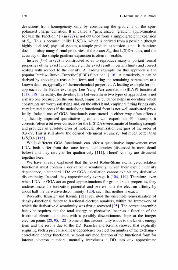
deviations from homogeneity only by considering the gradients of the spin-

polarized charge densities. It is called a “generalized” gradient approximation

because the function f (�) in (22) is not obtained from a simple gradient expansion

of Exc. This is because, unlike L(S)DA, which is derived from a possible (though

highly idealized) physical system, a simple gradient expansion is not. It therefore

does not obey many formal properties of the exact Exc that L(S)DA does, and the

accuracy of the simple gradient expansion is often miserable.

Instead, f (�) in (22) is constructed so as to reproduce many important formal

properties of the exact functional, e.g., the exact result in certain limits and correct

scaling with respect to the density. A leading example for this approach is the

popular Perdew–Burke–Ernzerhof (PBE) functional [116]. Alternatively, it can be

derived by choosing a reasonable form and fitting the remaining parameters to a

known data set, typically of thermochemical properties. A leading example for this

approach is the Becke exchange, Lee–Yang–Parr correlation (BLYP) functional

[117, 118]. In reality, the dividing line between these two types of approaches is not

a sharp one because, on the one hand, empirical guidance helps in deciding which

constraints are worth satisfying and, on the other hand, empirical fitting brings only

very limited success if the underlying functional form is not well-motivated phys-

ically. Indeed, use of GGA functionals constructed in either way often offers a

significantly improved quantitative agreement with experiment. For example, it

corrects (often a bit over-corrects) for the L(S)DA overestimate of bonding strength

and provides an absolute error of molecular atomization energies of the order of

0.3 eV. This is still above the desired “chemical accuracy,” but much better than

L(S)DA [115].

While different GGA functionals can offer a quantitative improvement over

LDA, both suffer from the same formal deficiencies (discussed in more detail

below) and they rarely differ qualitatively [111]. Therefore, they are discussed

together here.

We have already explained that the exact Kohn–Sham exchange-correlation

functional must contain a derivative discontinuity. Given their explicit density

dependence, a standard LDA or GGA calculation cannot exhibit any derivative

discontinuity. Instead, they approximately average it [104, 119]. Therefore, even

when LDA or GGA act as good approximations for ground state properties, they

underestimate the ionization potential and overestimate the electron affinity by

about half the derivative discontinuity [120], such that neither is exact.

Recently, Kraisler and Kronik [121] revisited the ensemble generalization of

density-functional theory to fractional electron numbers, within the framework of

which the derivative discontinuity was first discovered [95]. The correct ensemble

behavior requires that the total energy be piecewise-linear as a function of the

fractional electron number, with a possibly discontinuous slope at the integer

electron points [28, 95, 122]. Some of this discontinuity is due to the kinetic energy

term and the rest is due to the DD. Kraisler and Kronik showed that explicitly

requiring such a piecewise-linear dependence on electron number of the exchange-

correlation energy functional, without any modification of the functional form for

integer electron numbers, naturally introduces a DD into any approximate


exchange-correlation functional, even LDA and GGA. It does so by resulting in a

non-vanishing, spatially-uniform potential that leads to a different limiting value if

one approaches the integer number of electron from above or from below, which is

precisely the above-mentioned desired behavior of the DD. We also note that

Armiento and Kummel have recently shown that the conventional GGA form

allows one to construct an explicitly density dependent functional with a derivative

discontinuity that behaves much like the exact exchange discontinuity [123]. Yet, in

the following we only discuss calculations performed in the usual way, i.e., without

taking ensemble-DFT potential shifts into account and without the new GGA form.

However, one can still introduce, via other means, a rigid shift so as to account for

the difference between the HOMO and the ionization potential. If such a rigid shift

is allowed, how well do the results agree with experiment?

For simple semiconducting solids such as Si, it has long been known that all

salient features of the band structure corresponding to both filled and empty states,

save for the bandgap, are indeed captured rather accurately even with LDA, albeit

with an effective mass that is too small (see, e.g., [124, 125]). Furthermore, for Si

the LDA orbitals were found to possess a greater than 99% overlap with those

obtained from full diagonalization of the self-energy in the GW approximation

[40]. This is a first practical example for which we observe the general principle

laid down in the previous section – Kohn–Sham eigenvalues are not exactly quasi-

particle energies, but they are certainly not divorced from them, and they do provide

useful information. However, bulk Si is an exceptionally convenient example, for

which LDA results are very close to those obtained from the exact KS potential

[106]. Therefore, while confirmation of the principles of the previous section is

encouraging, is such performance to be generally expected from semi-local

functionals?

For finite systems the ionization potential can be determined independently,

using the same approximate density functional, simply by computing the total

energy difference between the system and its cation. The eigenvalue spectrum

can then be rigidly shifted, entirely from first principles, so as to set the HOMO

at the total-energy-difference ionization potential value [76, 126, 127]. In some

cases, this simple rigid-shift procedure is all that is needed to achieve satisfactory

agreement between ground-state DFT eigenvalues and the experimental UPS data.

An example is given by a UPS study of SimD�n gas-phase cluster anions [126, 128].

(The original study surveyed a broad range of 4 � m � 10 and 0 � n � 2. For

pedagogical reasons, we restrict our attention here to the subset m ¼ 4, 5, 6, and

n ¼ 0,1.) A fundamental problem in the study of clusters is that their geometrical

structure is generally unknown. Here, theory can assist by identifying low-lying

isomers using simulated-annealing that is based on first principles molecular-

dynamics [129, 130]. Agreement of the theoretical photoemission spectrum,

obtained from the predicted structure, with the experimentally measured spectrum

can then serve as evidence supporting the structure identification. We also note that

in studies of clusters it is known that statistical changes to the detailed cluster

geometry, due to finite-temperature effects, can be accounted for by averaging over


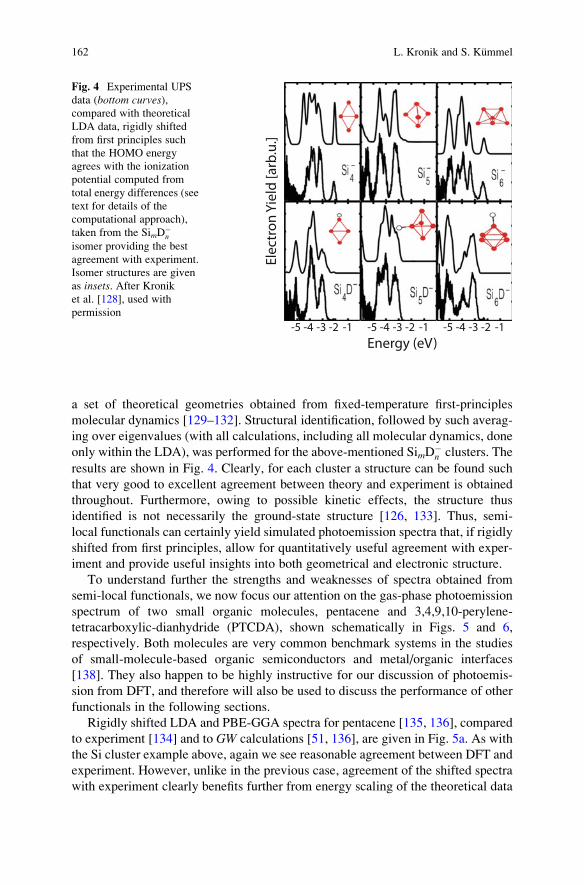
a set of theoretical geometries obtained from fixed-temperature first-principles

molecular dynamics [129–132]. Structural identification, followed by such averag-

ing over eigenvalues (with all calculations, including all molecular dynamics, done

only within the LDA), was performed for the above-mentioned SimD�n clusters. The

results are shown in Fig. 4. Clearly, for each cluster a structure can be found such

that very good to excellent agreement between theory and experiment is obtained

throughout. Furthermore, owing to possible kinetic effects, the structure thus

identified is not necessarily the ground-state structure [126, 133]. Thus, semi-

local functionals can certainly yield simulated photoemission spectra that, if rigidly

shifted from first principles, allow for quantitatively useful agreement with exper-

iment and provide useful insights into both geometrical and electronic structure.

To understand further the strengths and weaknesses of spectra obtained from

semi-local functionals, we now focus our attention on the gas-phase photoemission

spectrum of two small organic molecules, pentacene and 3,4,9,10-perylene-

tetracarboxylic-dianhydride (PTCDA), shown schematically in Figs. 5 and 6,

respectively. Both molecules are very common benchmark systems in the studies

of small-molecule-based organic semiconductors and metal/organic interfaces

[138]. They also happen to be highly instructive for our discussion of photoemis-

sion from DFT, and therefore will also be used to discuss the performance of other

functionals in the following sections.

Rigidly shifted LDA and PBE-GGA spectra for pentacene [135, 136], compared

to experiment [134] and to GW calculations [51, 136], are given in Fig. 5a. As with

the Si cluster example above, again we see reasonable agreement between DFT and

experiment. However, unlike in the previous case, agreement of the shifted spectra

with experiment clearly benefits further from energy scaling of the theoretical data

Elec

tron

Yie

ld [a

rb.u

.]

Energy (eV)5- 4- 3- 2- 1-5- 4- 3- 2- 1-5- 4- 3- 2- 1-

Fig. 4 Experimental UPS

data (bottom curves),compared with theoretical

LDA data, rigidly shifted

from first principles such

that the HOMO energy

agrees with the ionization

potential computed from

total energy differences (see

text for details of the

computational approach),

taken from the SimD�n

isomer providing the best

agreement with experiment.

Isomer structures are given

as insets. After Kroniket al. [128], used with

permission


(i.e., “stretching” of the energy axis) [135] by a factor of ~1.2. If this factor is

included (as also shown in Fig. 5a), quantitative agreement with experiment is

improved. This linear stretching is clearly in accordance with the above-mentioned

dominant nature of the linear corrections between self-energy and exchange-

correlation potential [101] and between Kohn–Sham eigenvalues and quasi-particle

energies [103, 135]. This combined “shift and stretch” procedure is often employed

a

b

Fig. 5 Gas-phase outer-valence photoemission spectroscopy of pentacene (shown schematically

in top right corner). (a) Experimental data (scanned in from Boschi et al. [134]), compared to

theoretically simulated data obtained from GW, LDA, PBE-GGA, and energy rescaled (by 20%)

PBE-GGA. (b) The same experimental data, compared to theoretically simulated data obtained

from the hybrid functional B3LYP in both OEP and GKS form, the hybrid functional PBE0 in

GKS form, and the PBE-based optimally-tuned range-separated hybrid functional with no

nonlocal short-range exchange and with 20% non-local short-range exchange. All spectra in

both (a) and (b) have been shifted rigidly so as to align the leading spectral peak. The size of

the shift needed to align the HOMO energy with the experimental ionization potential is indicated

by Δ to the right of each theoretical spectrum. See text for a complete description of the various

theoretical methods. The theoretical data were collected from Korzdorfer and Kummel, [135] and

Refaely-Abramson et al. [136], used with permission


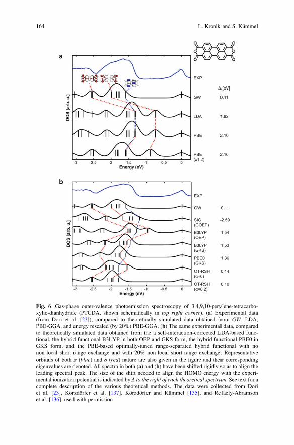
b

a

Fig. 6 Gas-phase outer-valence photoemission spectroscopy of 3,4,9,10-perylene-tetracarbo-

xylic-dianhydride (PTCDA, shown schematically in top right corner). (a) Experimental data

(from Dori et al. [23]), compared to theoretically simulated data obtained from GW, LDA,

PBE-GGA, and energy rescaled (by 20%) PBE-GGA. (b) The same experimental data, compared

to theoretically simulated data obtained from the a self-interaction-corrected LDA-based func-

tional, the hybrid functional B3LYP in both OEP and GKS form, the hybrid functional PBE0 in

GKS form, and the PBE-based optimally-tuned range-separated hybrid functional with no

non-local short-range exchange and with 20% non-local short-range exchange. Representative

orbitals of both π (blue) and σ (red) nature are also given in the figure and their corresponding

eigenvalues are denoted. All spectra in both (a) and (b) have been shifted rigidly so as to align the

leading spectral peak. The size of the shift needed to align the HOMO energy with the experi-

mental ionization potential is indicated by Δ to the right of each theoretical spectrum. See text for acomplete description of the various theoretical methods. The data were collected from Dori

et al. [23], Korzdorfer et al. [137], Korzdorfer and Kummel [135], and Refaely-Abramson

et al. [136], used with permission


semi-empirically in the literature (see, e.g., [139, 140]) when interpreting photo-

emission data with DFT based on semi-local functionals. It is often derided as a

heuristic “fudge-factor,” but here we see that it has a deep and well-justified

theoretical foundation. In fact it has even been recommended by Stowasser and

Hoffmann as a systematic means for quantitative interpretation of Kohn–Sham

eigenvalues obtained from the use of approximate exchange-correlation

functionals [81].

Our next prototypical molecule, PTCDA, shows that eigenvalue spectra from

semi-local functionals cannot always be remedied by a “shift and stretch” opera-

tion, as shown in Fig. 6a. By comparing LDA and PBE-GGA calculations with

gas-phase experimental photoemission data and with GW calculation, Dori

et al. [23] showed the DFT-based data to be in poor agreement with GW or

experiment even after a rigid shift. Most glaringly, the theoretical HOMO-1/

HOMO-2 peak (which is due to a doubly-degenerate eigenvalue) is found in a

region devoid of any meaningful signal in either GW or experiment. A key

observation for understanding the origin of the problem is that in PTCDA the

outer-valence orbitals can be broadly classified as π-orbitals, delocalized on the

perylene core, or σ-orbitals localized on the anhydride side groups. Representative

orbitals of either kind are also given in Fig. 6a and their corresponding eigenvalues

are denoted. Simultaneous description of localized and delocalized states is difficult

with semi-local functionals, also in the solid-state (see, e.g., [141, 142]) owing to

self-interaction errors [62].

What is the self-interaction error? In the Kohn–Sham equation (12) we have

somewhat arbitrarily selected to partition the consequences of electron–electron

interaction to a classical Coulomb part and an “everything else” exchange-

correlation part. As a result, an explicit classical electron–electron repulsion poten-

tial, namely the Hartree term, arises. As mentioned above, the latter is an essentially

classical expression that views the quantum charge probability distribution as a

classical distribution of charges. This, however, means that it is inherently in error,

because each electron is repelled from the total charge in the system, including a

spurious repulsion from itself. This effect is known as the self-interaction error and

was noted as early as 1934 by Fermi and Amaldi [143] in the context of Thomas–

Fermi theory [144, 145] – a “forerunner” of DFT. The spurious repulsion is

particularly easy to see in one-electron systems, where clearly there should be no

electron–electron repulsion at all, and yet the Hartree term is not zero. Because

electron–electron interaction is, in principle, handled exactly in DFT, whatever

error we are making in the Hartree term must be completely canceled out by the

exchange-correlation term. Unfortunately, complete error cancellation is

guaranteed for the exact exchange-correlation functional, but only partial cancel-

lation is obtained in either LDA or GGA.

Dori et al. found that the spectral distortions shown in Fig. 6a result primarily

from spurious positive energy shifts of the localized σ-orbitals. They therefore

hypothesized that these shifts reflect significant self-interaction errors: as the

electron is spuriously repelled from itself, it is destabilized, and therefore its

binding energy spuriously decreases. This error affects, in principle, all orbitals,


but self-repulsion is much more severe for the localized orbitals. As different

orbitals are affected in different ways, “stretching” provides no relief in this case.

Effects of a similar nature, but even greater quantitatively, were subsequently

observed for metal-phthalocyanine molecules [146–148].

Korzdorfer et al. [137] proved the self-interaction error hypothesis by quantify-

ing the per-orbital self-interaction error. Furthermore, they have shown that quan-

tification of the self-interaction error can be used as a predictive criterion for the

reliability of DFT calculations based on semi-local functionals: If the per-orbital

self-interaction error is constant, to within the accuracy sought, then the (shifted and

possibly stretched) eigenvalue spectrum will agree well with experiment. If not, the

spectrum will be distorted. This quantitative criterion was successfully used by

Rissner et al. to decide against the use of LDA/GGA in the theoretical study of

oligopyrimidines, where experimental data were not available [149].

To summarize, simulated photoemission data, constructed from the eigenvalues

of semi-local functionals, can be quantitatively useful. However, the two over-

whelming deficiencies of semi-local functionals [111] – self-interaction errors and

(in the standard implementation) a missing DD – limit its usefulness. Self-

interaction errors restrict the application range to systems where one does not

have to describe orbitals with greatly varying degrees of localization. For those

systems, the missing DD requires a rigid shift of the raw data, with the general

limitations of the Kohn–Sham potential typically requiring some further energy

scaling of the raw data.

6.2 Self-Interaction Correction

With self-interaction being a decisive criterion for the interpretability of DFT

eigenvalues, it is a natural question to ask whether one can eliminate the

one-electron self-interaction error completely. A famous scheme for self-

interaction correction (SIC) that achieves this has been suggested by Perdew and

Zunger [62]. The basic idea is quite transparent: From a given functional approx-

imation, here LSDA, subtract the terms that correspond to the one-electron self

interaction described in the previous section:

ESICxc n"; n#

� � ¼ ELSDAxc n"; n#

� �� Xσ¼", #

XNσ

i¼1

EH ni,σ½ � þ ELSDAxc ni,σ; 0½ ��

: ð23Þ

Here, ni,σ ¼ |φi,σ|2 are the orbital densities. The self-interaction terms are those in

parenthesis on the right-hand side of (23). Several general statements can be made

about the SIC that is defined in this way. For example, what are the formal grounds

of this functional? It is a non-empirical, explicitly orbital-dependent (and thus an

implicit) density functional. It is parameter-free and intuitively plausible. The

Perdew–Zunger type correction, when used in the Kohn–Sham context, leads to


the correct / � 1/r decay of the exchange-correlation potential, and this is gener-

ally beneficial for making �εH closer to I. However, the correct asymptotics alone

will not be enough for making �εH identical to I or for obtaining deeper lying

eigenvalues that reflect higher ionization potentials.

Quite generally, on looking closer, there are many subtleties buried in the

innocent looking (23). One should realize, e.g., that this SIC rests on identifying

orbitals with electrons [150]. This immediately brings about all the caveats

discussed in Sect. 5. In addition, the functional form is plausible, but there is no

way of systematically improving it or expanding on it. Its intuitive plausibility can

even be deceptive in some respects. For example, it has frequently been argued that

the SIC of (23) would vanish when applied to the ultimate functional, because by

definition the ultimate functional must be self-interaction free. Therefore, when

ELSDAxc in (23) would be replaced by the true, unknown exact Exc, then the correction

in parenthesis on the right-hand side of (23) should vanish. It has recently been

pointed out [151], though, that this need not be the case: Any ground-state density

functional and specifically the ultimate one is rigorously defined only on the domain

of ground-state densities. Almost all many-electron system orbital densities are not

ground-state densities, e.g., due to their nodal structure. Thus, strictly speaking (23)

uses the ground-state energy functional with input densities that are not in the set for

which the functional is defined. Furthermore, one could be tempted to use (23) as a

general definition and apply it not only to LSDA but also to other functionals, e.g.,

GGAs. However, it has also recently been argued here that this should be avoided

[152], because orbital densities are typically so different from ground-state densi-

ties that the gradient corrections that are reasonable when evaluated for ground-

state densities can take unphysical values when evaluated for orbital (i.e., excited-

state) densities.

The fact that makes the SIC interesting in the context of photoemission is

precisely the identification of orbitals with electrons that we mentioned above.

Perdew and Zunger have taken this argument to a formal level [62] and reasoned

that eigenvalues from a SIC calculation should benefit from a systematic cancella-

tion of errors. Remember that there is no formal equivalent to the original, Hartree–

Fock Koopmans’ in LSDA, i.e., no equality between eigenvalues and unrelaxed

excitation energies. Phrased slightly differently, this means that the unrelaxed

ionization energy is given by the negative of the DFT eigenvalue plus a “non-

Koopmans” correction. Of course the true ionization energies include relaxation

effects. Therefore, the relaxed ionization energy can be expressed as the DFT

eigenvalue plus the “non-Koopmans” correction plus a relaxation energy correc-

tion. The latter correction has the opposite sign of the former. Estimating both terms

for atomic densities, Perdew and Zunger showed that for LSDA the absolute value

of the “non-Koopmans” correction is much larger than the relaxation correction,

whereas for the SIC of (23) one can expect a reasonable cancellation between the

two. Therefore, SIC eigenvalues can be good approximations to relaxed ionization

potentials. This is a very attractive feature of the SIC, and not being tied to the


Koopmans’ theorem of Hartree–Fock theory thus turns into a very powerful

strength of DFT instead of a weakness.

Yet there are two reasons for being somewhat cautious about building too high

expectations on these considerations. The first is that it is not clear to what extent

the atom-based cancellation argument of [62] carries over to considerably more

complex molecules and solids. The second is rooted in (23) itself. As the SIC

energy depends on the orbitals directly, it is not straightforward to evaluate the

functional derivative of (14) that yields the exchange-correlation potential. There-

fore, the work of Perdew and Zunger and many SIC applications since then did not

use (23) with (14), but minimized the energy with respect to the orbitals, similar to

the procedure used in Hartree–Fock theory. When doing so, one has to face yet

another subtlety of (23): it is not invariant under a unitary transformation of the set

of occupied orbitals, i.e., different sets of occupied orbitals that yield the same

density lead to different energies. As a consequence of this unitary variance

problem, a direct minimization with respect to the orbitals leads to orbitals that

are not orthogonal. Orthogonality can be enforced via a set of Lagrangian multi-

pliers. This, however, leads to further questions, because with a matrix of Lagrang-

ian multipliers εiσjσ0 instead of eigenvalues εiσ, it is no longer clear which object may

serve as the approximation to the ionization potential. Traditionally the eigenvalues

of the matrix of Lagrange multipliers have been considered to be the equivalent of

the Kohn–Sham eigenvalues [153–155]. However, it has also been argued that the

eigenvalues of the matrix of Lagrange multipliers do not have any physical mean-

ing and that the diagonal elements of this matrix correspond to the orbital energies

[156]. Going deeper into the intricacies of SIC with orbital specific potentials is

beyond the scope of this chapter and the reader is referred to [111, 150] for a review

of different approaches to SIC. Here, we focus instead on how (23) can be related to

photoemission when it is used in a Kohn–Sham context.

Equation (14) can be evaluated for explicitly orbital dependent functionals with

the help of the optimized effective potential (OEP) equation [100, 111, 157–160].

The OEP combines two insights to build the local, multiplicative Kohn–Sham

potential. First, the Kohn–Sham orbitals are themselves functionals of the density

and, second, the functional derivative of (14) can be evaluated by using the chain

rule of functional derivatives. The chain rule allows for turning the derivative of the

energy with respect to the density into one with respect to the orbitals, multiplied by

a derivative of the orbitals with respect to the density. The latter can be evaluated by

linear response theory. A comprehensive review of OEP techniques is given in

[111]. Constructing the local Kohn–Sham exchange correlation potential via the

OEP approach for the SIC is numerically tedious but possible [161]. It leads to

HOMO eigenvalues that often compare to first ionization potentials more favorably

than those obtained from semi-local functionals. The difference between the

LSDA-SIC HOMO eigenvalue and the experimental ionization potential is, e.g.,

0.14 eV, 0.82 eV, and�0.27 eV for the molecules CH4, H2O, and CO, respectively.

This is a huge improvement over LSDA, for which the corresponding values are

�4.90 eV, �5.17 eV, and �6.66 eV. However, the problem with straightforward

OEP calculations for the LSDA-SIC functional is that the calculations converge


very poorly – an effect that is to a considerable extent a consequence of the unitary

variance problem. Therefore systematic tests or results for larger molecules are not

available.

The problem can be considerably reduced by taking the unitary variance degree

of freedom into account explicitly in the OEP equation. This generalized OEP

(GOEP) approach allows for SIC calculations that converge much more rapidly and

therefore also allow for Kohn–Sham SIC calculations for larger molecules. The

theory of GOEP has been described in detail in [150]. Therefore, here we focus on

the relation to photoemission. Returning to the previously mentioned small mole-

cules reveals the drawback of going from OEP to GOEP: for CH4, H2O, and CO the

differences between the GOEP HOMO eigenvalue and the experimental ionization

potential are 1.63, 2.31, and �0.27 eV, respectively. These numbers are typical. In

contrast to most other DFT approximations, which lead to eigenvalues that are too

high, SIC eigenvalues are too negative, and GOEP enhances this trend over OEP. In

some sense, SIC overcorrects the errors of LSDA, and thus overestimates ionization

potentials.

The true strength of GOEP-SIC in practical applications thus lies not in the

accurate prediction of absolute ionization energies, but in predicting orbital order-

ings and the relative eigenvalue spectrum, e.g., the ionization energies up to a rigid

shift. The relative eigenvalue spectrum of GOEP-SIC provides, e.g., a very reason-

able estimate for the upper parts of the photoemission spectrum even for “difficult”

cases such as the previously discussed PTCDAmolecule [137], as shown in Fig. 6b.

Note that the GOEP-SIC calculation would still benefit from “stretching,” for the

same reasons given above, but the spectral distortion due to self-interaction errors

has been removed.

A yet more notable use of GOEP-SIC has been the prediction of the intensity

patterns observed in angularly resolved photoemission spectroscopy (ARPES). The

relation between orbitals and ARPES can be understood based on the equations of

Sect. 2. Assuming the final state γk to be a plane wave, approximating the other

wavefunctions by Slater determinants, further assuming that relaxation effects are

small so that initial and final Slater-determinant are built from the same set of

orbitals, and taking the emission intensity as proportional to the matrix element of

(4) will lead to the relation [162]

I kx; ky;Ekin

� � / ��φiσ kð Þ��2��k¼const

��A � k��2: ð24Þ

As previously defined, k is the momentum of the outgoing electron (plane wave).

The power of (24) lies in the observation that it builds a direct connection between

the measured photoemission intensity and the Fourier transform, i.e., momentum

space representation, of a molecular orbital. The factor |A � k|2 is known both

experimentally and theoretically. Therefore, (24) allows for a direct comparison

of theory and experiment as follows. (1) Calculate, via Fourier-transformation, the

momentum representation of a molecular orbital. (2) For a given value of k, i.e., acertain kinetic energy, obtain a two-dimensional cut through the orbital

(in momentum space) by plotting φiσ(k) as a function of kx and ky (the value of kz


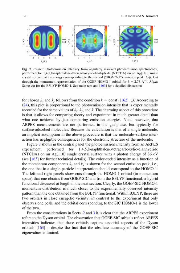
for chosen kx and ky follows from the condition k ¼ const) [162]. (3) According to

(24), this plot is proportional to the photoemission intensity that is experimentally

recorded for the same values of kx, ky, and k. The charming aspect of this procedure

is that it allows for comparing theory and experiment in much greater detail than

what one achieves by just comparing emission energies. Note, however, that

ARPES measurements are not performed in the gas-phase, but typically for

surface-adsorbed molecules. Because the calculation is that of a single molecule,

an implicit assumption in the above procedure is that the molecule–surface inter-

action has negligible consequences for the electronic structure of the molecule.

Figure 7 shows in the central panel the photoemission intensity from an ARPES

experiment, performed for 1,4,5,8-naphthalene-tetracarboxylic-dianhydride

(NTCDA) on an Ag(110) single crystal surface with a photon energy of 36 eV

(see [163] for further technical details). The color-coded intensity as a function of

the momentum components kx and ky is shown for the second emission peak, i.e.,

the one that in a single-particle interpretation should correspond to the HOMO-1.

The left and right panels show cuts through the HOMO-1 orbital (in momentum

space) that one obtains from GOEP-SIC and from the B3LYP functional, a hybrid

functional discussed at length in the next section. Clearly, the GOEP-SIC HOMO-1

momentum distribution is much closer to the experimentally observed intensity

pattern than the one obtained from the B3LYP functional. Within B3LYP, there are

two orbitals in close energetic vicinity, in contrast to the experiment that only

observes one peak, and the orbital corresponding to the SIC HOMO-1 is the lower

of the two.

From the considerations in Sects. 2 and 3 it is clear that the ARPES experiment

refers to the Dyson orbital. The observation that GOEP-SIC orbitals reflect ARPES

intensities indicates that these orbitals capture essential aspects of the Dyson

orbitals [163] – despite the fact that the absolute accuracy of the GOEP-SIC

eigenvalues is limited.

Fig. 7 Center: Photoemission intensity from angularly resolved photoemission spectroscopy,

performed for 1,4,5,8-naphthalene-tetracarboxylic-dianhydride (NTCDA) on an Ag(110) single

crystal surface, at the energy corresponding to the second (“HOMO-1”) emission peak. Left: Cut

through the momentum representation of the GOEP HOMO-1 orbital for k ¼ 2.73 Å�1. Right:Same cut for the B3LYP HOMO-1. See main text and [163] for a detailed discussion


6.3 Conventional Hybrid Functionals

The next functional class we examine is that of hybrid functionals [111], pioneered

by Becke [164, 165] some 20 years ago as a means of overcoming some of the

remaining limitations of GGA functionals. Generally, conventional hybrid func-

tionals incorporate a fixed fraction of exact-exchange energy, defined in terms of

the Fock integral, given (in atomic units) by

E exactx ¼ � 1

2

Xσ¼", #

XNσ

i, j¼1

Z Zφ�i,σ rð Þφ�

j,σ r0ð Þφj,σ rð Þφi,σ r0ð Þr-r0j j d3r0d3r, ð25Þ

which is familiar from Hartree–Fock theory. The exchange-correlation energy is

then expressed as

Ehybxc ¼ bE exact

x þ 1� bð ÞE appx þ E app

c , ð26Þ

where b is the exact-exchange fraction and the superscripts ‘hyb’ and ‘app’ denote

the hybrid functional and the approximate (typically semi-local) exchange and

correlation functionals from which it is constructed. As with GGA functionals,

hybrid functionals can be constructed either non-empirically or semi-empirically.

In the non-empirical hybrid functional based on the above-mentioned PBE

GGA-functional (called PBE0 to emphasize the lack of empirical parameters)

[166–168], Eappx and Eapp

c are taken from the PBE functional. Therefore b is the

only free parameter and it is determined from non-empirical (though still heuristic)

considerations to be 0.25 [166]. In the semi-empirical hybrid functional based on

the BLYP GGA-functional, the fraction of exact exchange, as well as two addi-

tional parameters in the underlying GGA expressions, are left free and are deter-

mined by fitting to thermochemical data, leading to the functional name –

B3LYP [169].

While hybrid functionals are also of growing influence in solid-state physics

(see, e.g., [170, 171]), they have particularly left their mark in organic chemistry

[29]. This is because they offer a further and significant reduction of errors with

respect to GGA functionals. For example, for the formation enthalpies of the G3 set

of thermochemical data, the mean error is 0.94 eV with PBE-GGA, but only 0.2 eV

with the PBE0 hybrid functional, and 0.15 eV with B3LYP, respectively

[172]. From a fundamental point of view, there are several perspectives to ratio-

nalize why one would wish to use a fraction of exact exchange, rather than all of

it. One formal justification, dating back to Becke’s original work [164], is grounded

in the adiabatic connection theorem, the discussion of which is outside the scope of

this chapter (but see [111] for an overview). For our purposes, it suffices to note that

full exact exchange would necessarily require a highly non-local correlation expres-

sion, which at present is unknown. Retaining only a fraction of it provides for a

reasonable balance between enjoying its advantages and retaining a simple, semi-

local correlation functional.


To be used within the Kohn–Sham scheme, the exchange-correlation potential

needs to be determined from the exchange-correlation energy of (26) via a func-

tional derivative with respect to the electron density. Such derivation is certainly

possible. If the orbital-dependent Fock expression is taken as an implicit functional

of the density, the functional derivative can be evaluated using the OEP procedure

explained in the previous section. However, this is rarely done in practice. Instead,

because the Fock-exchange depends explicitly on the orbitals, the energy is derived

with respect to the latter, leading to a non-local, Fock-operator potential. The name

“hybrid functionals” is derived from this property, because such evaluation was

originally understood to be a mixture of the Kohn–Sham and Hartree–Fock world

views [164].

A more modern perspective is to view such non-local potential operators as

indeed being outside the scope of the Kohn–Sham equation, but well within formal

DFT nevertheless, by virtue of the generalized Kohn–Sham equation [173, 174]. As

discussed above, the original Kohn–Sham scheme relies on the Hohenberg–Kohn

theorem to establish mapping into a system that, by virtue of its non-interacting-

particle nature, could be described by a single Slater determinant. In a seminal

article, Seidl et al. [173] pointed out that one could equally well rely on the

Hohenberg–Kohn theorem to map the real system into any interacting model

system that can still be represented by a single Slater determinant, but will no

longer necessarily be described by a strictly local potential. They proved that such

an alternate mapping can be achieved in practice by defining an energy functional,

S [{φi}], of the orbitals {φi} comprising the Slater determinant of the model system,

and expressing the total energy as a sum of S [{φi}], the ion–electron attraction, and

a “remainder” term. One next seeks the Slater determinant that minimizes this form

of the energy functional while yielding the density of the original system. The

minimizing orbitals then play a role analogous to that of the Kohn–Sham orbitals.

A thorough discussion of this procedure, from various perspectives, can be found in

the original work of Seidl et al., as well as in several review articles [111, 112, 175].

It leads to a generalized Kohn–Sham (GKS) equation in the form

O S φif g½ � þ vext rð Þ þ vR rð Þ� �

φj rð Þ ¼ εjφj rð Þ, ð27Þ

where Oˆ S [{φi}] is a generally non-local, orbital-specific operator that depends on

the choice of S [�] but not on the system specifics, and

vR rð Þ � δRS n½ �δn rð Þ ð28Þ

is the “remainder potential,” a multiplicative potential which is a functional of the

density, that is determined from a functional derivative of a “remainder” energy

term, RS[n].Formally, both the KS and the GKS maps are exact [173]. However, whereas

there is only one KS map, there exist a multitude of GKS maps, depending on the


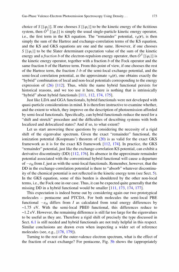
choice of S [{φi}]. If one chooses S [{φi}] to be the kinetic energy of the fictitious

system, then Oˆ S [{φi}] is simply the usual single-particle kinetic energy operator,

i.e., the first term in the KS equation. The “remainder” potential, vR(r), is then

simply the sum of the Hartree and exchange-correlation terms of the KS equation,

and the KS and GKS equations are one and the same. However, if one chooses

S [{φi}] to be the Slater determinant expectation value of the sum of the kinetic

energy and a fraction b of the electron-repulsion energy operator, then Oˆ S [{φi}] is

the kinetic energy operator, together with a fraction b of the Fock operator and the

same fraction b of the Hartree term. From this point of view, if one chooses the rest

of the Hartree term, the fraction 1-b of the semi-local exchange potential, and the

semi-local correlation potential, as the approximate vR(r), one obtains exactly the

“hybrid” combination of local and non-local potentials corresponding to the energy

expression of (26) [112]. Thus, while the name hybrid functional persists for

historical reasons, and we too use it here, there is nothing that is intrinsically

“hybrid” about hybrid functionals [111, 112, 174, 175].

Just like LDA and GGA functionals, hybrid functionals were not developed with

quasi-particle considerations in mind. It is therefore instructive to examine whether,

and the extent to which, they improve on the description of photoemission afforded

by semi-local functionals. Specifically, can hybrid functionals reduce the need for a

“shift and stretch” procedure and the difficulties of describing systems with both

localized and delocalized states? And if so, to what extent?

Let us start answering these questions by considering the necessity of a rigid

shift of the eigenvalue spectrum. Given the exact “remainder” functional, the

ionization potential (Koopmans’) theorem of (20) is as valid for the exact GKS

framework as it is for the exact KS framework [112, 174]. In practice, the GKS

“remainder” potential, just like the exchange-correlation KS potential, can exhibit a

derivative discontinuity (DD) [112, 176]. Its absence in the approximate remainder

potential associated with the conventional hybrid functional will cause a departure

of�εH from I, just as with the semi-local functionals. Remember, however, that the

DD in the exchange-correlation potential is there to “absorb” whatever discontinu-

ity of the chemical potential is not reflected in the kinetic energy term (see Sect. 5).

In the GKS equation, some of this burden is shouldered by the other non-local

terms, i.e., the Fock one in our case. Thus, it can be expected quite generally that the

missing DD in a hybrid functional would be smaller [111, 173, 174, 177].

This expectation is indeed borne out by considering again our two prototypical

molecules – pentacene and PTCDA. For both molecules the semi-local PBE

functional �εH differs from I as calculated from total energy differences by

~1.75 eV. With the semi-local PBE0 functional, this differences reduce to

~1.2 eV. However, the remaining difference is still far too large for the eigenvalues

to be useful as they are. Therefore a rigid shift of precisely the type discussed in

Sect. 6.1 is still needed and hybrid functionals are not truly helpful in this respect.

Similar conclusions are drawn even when inspecting a wider set of reference

molecules (see, e.g., [178, 179]).

Turning to the rest of the outer-valence electron spectrum, what is the effect of

the fraction of exact exchange? For pentacene, Fig. 5b shows the (appropriately


shifted) eigenvalue spectrum obtained with the B3LYP and PBE0 hybrid func-

tionals [135, 136]. For this system, where the shifted spectrum from the PBE

functional already provided a qualitatively useful answer, the hybrid functional

spectrum provides further improvement by essentially eliminating the need for a

“stretch factor.” We emphasize strongly that this is a direct consequence of using

the GKS approach, i.e., a non-local Fock-operator potential. To prove that, Fig. 5b

also shows the spectrum obtained from the B3LYP functional, but with a KS

potential obtained from solving the OEP equation [135]. Clearly, these results do

need stretching, despite the underlying use of hybrid functional energy expression,

and are in fact quite similar to those obtained with PBE-GGA.

Korzdorfer and Kummel rationalized the stretching afforded by using the GKS

procedure [135]. They argued that, if the differences in the KS and GKS orbitals are

ignored, then the difference between each GKS and corresponding KS eigenvalue

can be viewed in terms of first-order perturbation theory involving the difference

between the Fock and semi-local exchange. They suggested that this first-order

correction mimics successfully the above-mentioned first-order correction between

Kohn–Sham values and ionization energies due to Chong et al. [103]. We note that

the hybrid first-order correction only involves a term related to fractional non-local

exchange, whereas the Chong et al. correction involves a non-local exchange term

as well as a correlation term. However, using only a fraction of Fock exchange so as

to affect a reasonable balance between exchange and correlation is precisely the

rationale of the hybrid functional. Indeed, if the photoemission spectrum of a hybrid

functional is studied as a function of the Fock fraction b, it is discovered that the

standard fraction, conceived in the design of the functional from energetic consid-

erations is also best for the photoemission spectrum [135, 180]. A different,

complementary perspective for the improved “stretch” afforded by the hybrid

functional calculation is that the non-local potential is more likely to mimic well

the self-energy operator, which is itself non-local [111, 112, 173, 181, 182]. While

the non-local potential still cannot be equivalent to the self-energy operator, as it is

not frequency-dependent, it certainly constitutes a step in the right direction.

An even more dramatic improvement of hybrid functionals, employed using the

GKS scheme, over semi-local ones is found for our second prototypical system –

PTCDA – as shown in Fig. 6b. Clearly, the spectral distortion is strongly reduced.

In particular, the leading spurious peak obtained from the PBE-GGA calculation is

gone and eigenvalues of localized states, spuriously pushed too high by the GGA

calculation, are returned to lower energies where their resemblance to experimental

and/or GW data is greatly improved. Again, this improvement is not fully obtained

if one employs the hybrid functional using the OEP procedure, as also shown in

Fig. 6b. Not only is “stretching” needed with the OEP procedure, as explained

above, but in fact some of the desirable orbital ordering is lost. A similar improve-

ment of conventional hybrid functionals over semi-local ones has been repeatedly

found for porphyrins and phthalocyanins – a different class of prototypical mole-

cules comprising both localized and delocalized states; see, e.g., [147, 148, 180,

183–185]. For such systems, highly detailed comparisons to sufficiently-resolved

experimental data often reveal that some further quantitative improvement can be


obtained from a GW calculation (see, e.g., [186, 187]). Nevertheless, the degree of

quantitative agreement between the conventional hybrid spectrum and the GWspectrum is often as good as the experimental resolution.

This success of the hybrid functional approach is not at all a trivial finding: we

have argued above that these distortions result from self-interaction errors, but

hybrid functionals are certainly not self-interaction free! Complete cancellation of

the self-interaction in the Hartree term would require the full Fock exchange, not

just a fraction of it, along with a self-interaction free correlation potential. Neither

condition is met in a conventional hybrid functional. One can only conclude that

again a reasonable balance between exchange and correlation is struck by using a

fraction of Fock exchange. While this balance cannot and does not eliminate self-

interaction errors (as also obvious from the results of Fig. 7 and the above discus-

sion), it does mitigate them to a point where the eigenvalue spectrum more closely

resembles the spectrum obtained from many-body perturbation theory, to the point

where quantitative or close-to-quantitative agreement of the shifted eigenvalue

spectrum with experiment is often found.

To summarize, conventional hybrid functionals differ from semi-local ones not

only in the form of the exchange-correlation energy but also in that they are usually

evaluated using a non-local potential operator within the generalized Kohn–Sham

scheme. These two differences reduce, but far from eliminate, the need for a rigid

shift of the eigenvalue spectrum. They do mitigate very strongly, often quantita-

tively, the need for spectral “stretching” and the distortions arising from self-

interaction errors.

6.4 Range-Separated Hybrid Functionals

A disadvantage that is common to all preceding classes of functionals is the

incorrect prediction of the ionization potential, I, as well as the electron affinity,

A. For gas-phase systems, we have already mentioned that these quantities can

easily be calculated from total energy differences. Therefore one could argue that

obtaining an eigenvalue spectrum that is similar to photoemission data, up to a rigid

shift (as with the self-interaction-corrected or hybrid functionals of the preceding

two sections), is quite sufficient. However, significant further advantages can be

gained if indeed I and A can be equated with �εH and �εL, respectively. Forexample, accurate positioning of frontier orbitals is essential for transport calcula-

tions and therefore gross errors in the calculation of conductance can ensue from the

use of approximate DFT forms [188–190]. More importantly for the gas phase, if

we are truly to mimic the results of many-body perturbation theory with DFT, one

would prefer to retain, if possible, an intuitive connection between single-particle

energy levels and quasi-particle excitations. This is especially so if one also wishes

to consider optical excitations, which can be thought of as simultaneous excitation

of a quasi-electron and a quasi-hole [44, 191]. Obtaining the correct fundamental

gap is in fact crucial for describing the electron–hole interaction in terms of an


exciton binding energy, as one does in many-body perturbation theory [112] and in

particular indispensable for the description of charge transfer excitations using

linear-response within TDDFT [192–196].

We have already explained in Sect. 5 that equating �εL with A is not possible

within the Kohn–Sham scheme owing to the usually non-negligible DD. We have

also argued in Sect. 6.3 that within the generalized Kohn–Sham scheme there is

hope for reducing the magnitude of the DD, but that in practice conventional hybrid

functionals do not achieve this lofty goal. Stein et al. [197] observed that in the gas

phase the asymptotic potential must play a crucial role in the energetics of electron

addition and removal. However, an asymptotically correct 1/r Coulomb potential is

obtained only if the full Fock exchange cancels out the self-interaction in the

Hartree term. As explained in Sect. 6.3, in conventional hybrid functionals only a

fraction of the Fock exchange is used. Increasing that fraction would disrupt the

hard-earned and delicate balanced between exchange and correlation. In order to

escape this conundrum, then, we must step out of the conventional hybrid func-

tional framework.

One appealing idea is the range-separated hybrid (RSH) functional, proposed by

Savin and co-workers [198]. In the simplest realization of this idea, the repulsive

Coulomb potential is split into a long-range (LR) and short-range (SR) term, e.g., via

1=r ¼ erf γrð Þ=rþerfc γrð Þ=r, ð29Þ

where erf(�) and erfc(�) denote the standard and complementary error functions,

respectively, and γ is a range-separation parameter. The SR and LR components are

taken together in the usual way for the Hartree term, yielding the standard Hartree

potential, but the components are treated differently in the generation of the

exchange term. The LR part is treated via a Fock exchange term, but the SR part

is treated using semi-local exchange. A conventional semi-local correlation expres-

sion is used throughout. Minimization of the ensuing exchange-correlation energy

expression with respect to orbitals then leads to

�∇2

2þ vext rð Þ þ vH n½ �; rð Þ þ v lr, γ

F þ vsr, γx n½ �; rð Þ þ v slc n½ �; rð Þ �

φi rð Þ

¼ εiφi rð Þ, ð30Þ

where v lr, γF is a long-range Fock-like operator, namely

v lr, γF φi rð Þ ¼ �

Xj

φj rð ÞZ

dr0erf γ

��r� r0��

r� r0j j φ�j r0ð Þφi r

0ð Þ, ð31Þ

vsr;γx ([n]; r) is the multiplicative potential arising from the semi-local treatment

of the SR exchange, and vslc ([n]; r) is the (multiplicative) correlation potential.

The logic of the range-separation idea (which is rooted in even earlier efforts to

wed DFT with the configuration-interaction method [199, 200]) is that the relative


importance of exchange and correlation is different for different interaction ranges.

Our above quandary of the two seemingly contradictory requirements is solved,

then, by “partition of labor.” The exact LR Fock exchange is in charge of enforcing

the correct form of the asymptotic potential. At the same time, the semi-local SR

exchange is in charge of maintaining the delicate balance with correlation.

It is readily established that the RSH construct of (30) is yet another special case

of the generalized Kohn–Sham approach [112]. To show that, we choose S[{φi}] to

be the Slater-determinant expectation value of the sum of the kinetic energy and the

long-range electron-repulsion energy operator, erf(γr)/r. This yields the usual

kinetic energy operator, together with the LR fraction of the Fock operator and

the Hartree term. Our specific choice of the “remainder potential,” νR(r), is then thesum of the SR Hartree term, the local potential derived from the SR exchange term,

and a standard correlation potential.

In order to use the RSH scheme, one must still decide on the choice for the range-

separation parameter, γ. Physically, 1/γ can be viewed as the range below which the

exchange is dominated by its SR contribution and above which the exchange is

dominated by its LR contribution. To realize that the choice of γ plays a crucial rolein the success of the approach, it suffices to consider its limits. For γ ! 0, (30)

reduces to the usual Kohn–Sham equation (12), with a semi-local functional. For

γ ! 1, it reduces to the Hartree–Fock equation with added semi-local correlation.

The former has already been noted to underestimate the fundamental gap severely

and the latter is well-known to overestimate it severely [111]. How can we tell,

then, in a predictive manner, which values of γ we should choose to use?

Clearly, just as in some semi-local functionals and conventional hybrid func-

tionals, one can opt to proceed semi-empirically. This means that γ, possiblytogether with other free parameters in the semi-local exchange and correlation

terms, can be fitted based on appropriate reference data. In fact, most modern

RSH functionals are constructed in this way – see, e.g., [201–207]. However,

both formal considerations [208] and practical simulations for the homogeneous

electron gas problem [209] show that obtaining accurate results often requires

significantly different values of γ. In fact, γ itself can be viewed as functional of

the density [208], on which very little is known.

Within the range-separated hybrid functional approach, an essential concept for

overcoming this difficulty is the use of non-empirical, system-specific optimal

tuning to determine the range separation parameter. This allows us to overcome

the absence of a universal, system-independent value for the range-separation

parameter, γ. For photoemission, one would like to identify the HOMO orbital

with the ionization potential, i.e., to uphold the ionization potential theorem of (20),

�εH ¼ I. Therefore, one can employ the concept of optimal tuning in practice by

actively seeking the value of γ for which (20) is obeyed [209]. This means that we

seek γ for which the negative of the HOMO energy is the same as the ionization

potential determined from the total energy difference between cation and neutral.

This approach was indeed found to be very successful in the prediction of ionization


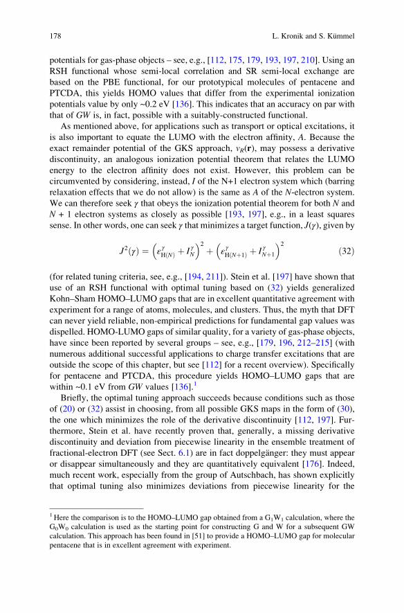
potentials for gas-phase objects – see, e.g., [112, 175, 179, 193, 197, 210]. Using an

RSH functional whose semi-local correlation and SR semi-local exchange are

based on the PBE functional, for our prototypical molecules of pentacene and

PTCDA, this yields HOMO values that differ from the experimental ionization

potentials value by only ~0.2 eV [136]. This indicates that an accuracy on par with

that of GW is, in fact, possible with a suitably-constructed functional.

As mentioned above, for applications such as transport or optical excitations, it

is also important to equate the LUMO with the electron affinity, A. Because the

exact remainder potential of the GKS approach, vR(r), may possess a derivative

discontinuity, an analogous ionization potential theorem that relates the LUMO

energy to the electron affinity does not exist. However, this problem can be

circumvented by considering, instead, I of the N+1 electron system which (barring

relaxation effects that we do not allow) is the same as A of the N-electron system.

We can therefore seek γ that obeys the ionization potential theorem for both N and

N + 1 electron systems as closely as possible [193, 197], e.g., in a least squares

sense. In other words, one can seek γ that minimizes a target function, J(γ), given by

J2 γð Þ ¼ εγH Nð Þ þ I γN

� �2

þ εγH Nþ1ð Þ þ I γNþ1

� �2

ð32Þ

(for related tuning criteria, see, e.g., [194, 211]). Stein et al. [197] have shown that

use of an RSH functional with optimal tuning based on (32) yields generalized

Kohn–Sham HOMO–LUMO gaps that are in excellent quantitative agreement with

experiment for a range of atoms, molecules, and clusters. Thus, the myth that DFT

can never yield reliable, non-empirical predictions for fundamental gap values was

dispelled. HOMO-LUMO gaps of similar quality, for a variety of gas-phase objects,

have since been reported by several groups – see, e.g., [179, 196, 212–215] (with

numerous additional successful applications to charge transfer excitations that are

outside the scope of this chapter, but see [112] for a recent overview). Specifically

for pentacene and PTCDA, this procedure yields HOMO–LUMO gaps that are

within ~0.1 eV from GW values [136].1

Briefly, the optimal tuning approach succeeds because conditions such as those

of (20) or (32) assist in choosing, from all possible GKS maps in the form of (30),

the one which minimizes the role of the derivative discontinuity [112, 197]. Fur-

thermore, Stein et al. have recently proven that, generally, a missing derivative

discontinuity and deviation from piecewise linearity in the ensemble treatment of

fractional-electron DFT (see Sect. 6.1) are in fact doppelganger: they must appear

or disappear simultaneously and they are quantitatively equivalent [176]. Indeed,

much recent work, especially from the group of Autschbach, has shown explicitly

that optimal tuning also minimizes deviations from piecewise linearity for the

1Here the comparison is to the HOMO–LUMO gap obtained from a G1W1 calculation, where the

G0W0 calculation is used as the starting point for constructing G and W for a subsequent GW

calculation. This approach has been found in [51] to provide a HOMO–LUMO gap for molecular

pentacene that is in excellent agreement with experiment.


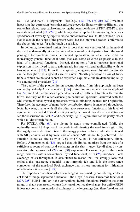
[N � 1,N] and [N,N + 1] segments – see, e.g., [112, 136, 176, 216–220]. We note

in passing that correction terms that enforce piecewise linearity offer a different, but

somewhat related, approach to improving the correspondence of DFT HOMO to the

ionization potential [221–226], which may also be applied to improving the corre-

spondence of lower-lying eigenvalues to photoemission results. Its detailed discus-

sion is outside the scope of the present work, but the interested reader is referred to

the above references for a thorough discussion.

Importantly, the optimal tuning idea is more than just a successful mathematical

device. Fundamentally, it can be viewed as a significant departure from the usual

paradigm for functional construction and application, in which one seeks an

increasingly general functional form that can come as close as possible to the

ideal of a universal functional. Instead, the notion of an all-purpose functional

expression is sacrificed so as to gain greatly in simplicity and applicability with no

loss of accuracy [112]. From this perspective, range-separated hybrid functionals

can be thought of as a special case of a new, “fourth generation” class of func-

tionals, which are not and cannot be expressed explicitly, but are defined implicitly

via a numerical procedure [211].

The quality of the photoemission spectra obtained from this approach has been

studied by Refaely-Abramson et al. [136]. Returning to the pentacene example of

Fig. 5b, we find that the above procedure is indeed sufficient to retain the quanti-

tative accuracy of the outer-valence photoemission spectrum, achieved with the

SIC or conventional hybrid approaches, while eliminating the need for a rigid shift.

Therefore, the accuracy of many-body perturbation theory is matched throughout.

Note, however, that as with all the other above-surveyed functionals, this level of

agreement is expected to (and does) gradually deteriorate for deeper excitations –

see the discussion in Sect. 5 and especially Fig. 3. Again, this can be partly offset

with a milder stretch factor.

For PTCDA (Fig. 6b), the picture is again more complicated. While the

optimally-tuned RSH approach succeeds in eliminating the need for a rigid shift,

the largely successful description of the energy position of localized states, obtained

with SIC, conventional hybrids, and of course GW, is not fully achieved. The

situation is not as dire as with LDA or GGA, but is not satisfactory either.

Refaely-Abramson et al. [136] argued that this limitation arises from the lack of a

sufficient amount of non-local exchange in the short-range. Recall that, by con-

struction, the approach of (29) and (30) suppresses Fock-exchange in the short-

range, whereas with a conventional hybrid functional, as in (26), non-local Fock

exchange exists throughout. It also stands to reason that, for strongly localized

orbitals, the long-range potential is not strongly felt and it is the short-range

component of the non-local Fock exchange that is more important for mitigation

of self-interaction errors [147].

The importance of SR non-local exchange is confirmed by considering a differ-

ent kind of range-separated functional – the Heyd–Scuseria–Ernzerhof functional

[227, 228]. HSE is similar to the conventional hybrid functional PBE0 in the short

range, in that it possesses the same fraction of non-local exchange, but unlike PBE0

it does not contain any non-local exchange in the long-range (and therefore does not


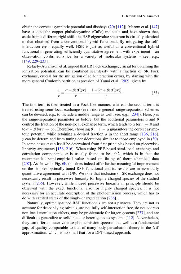
obtain the correct asymptotic potential and disobeys (20) [112]). Marom et al. [147]

have studied the copper phthalocyanine (CuPc) molecule and have shown that,

aside from a different rigid shift, the HSE eigenvalue spectrum is virtually identical

to that obtained from a conventional hybrid functional. By mitigating the self-

interaction error equally well, HSE is just as useful as a conventional hybrid

functional in generating sufficiently quantitative agreement with experiment – an

observation confirmed since for a variety of molecular systems – see, e.g.,

[149, 229–233].

Refaely-Abramson et al. argued that LR Fock exchange, crucial for obtaining the

ionization potential, can be combined seamlessly with a fraction of SR Fock

exchange, crucial for the mitigation of self-interaction errors, by starting with the

more general Coulomb partition expression of Yanai et al. [202], given by

1

r¼ αþ βerf γrð Þ

rþ 1� αþ βerf γrð Þ½ �

r: ð33Þ

The first term is then treated in a Fock-like manner, whereas the second term is

treated using semi-local exchange (even more general range-separation schemes

can be devised, e.g., to include a middle range as well; see, e.g., [234]). Here, γ isthe range-separation parameter as before, but the additional parameters α and βcontrol the fraction of the non-local exchange term, which tends to α for r ! 0 and

to α + β for r ! 1. Therefore, choosing β ¼ 1 � α guarantees the correct asymp-

totic potential while retaining a desired fraction α in the short range [136, 216].

γ can be determined from tuning considerations similar to those employed in (30).

In some cases α can itself be determined from first principles based on piecewise-

linearity arguments [136, 216]. When using PBE-based semi-local exchange and

correlation components, α is usually found to be ~0.2, which is in fact the

recommended semi-empirical value based on fitting of thermochemical data

[207]. As shown in Fig. 6b, this does indeed offer further meaningful improvement

on the simpler optimally-tuned RSH functional and its results are in essentially

quantitative agreement with GW. We note that inclusion of SR exchange does not

necessarily result in piecewise linearity for highly charged species of the studied

system [235]. However, while indeed piecewise linearity in principle should be

observed with the exact functional also for highly charged species, it is not

necessary for an accurate description of the photoemission process, which has to

do with excited states of the singly-charged cation [236].

Naturally, optimally-tuned RSH functionals are not a panacea. They are not as

accurate for deeper-lying orbitals, are not fully self-interaction free, do not address

non-local correlation effects, may be problematic for larger systems [237], and are

difficult to generalize to solid-state or heterogeneous systems [112]. Nevertheless,

they can offer an outer-valence photoemission spectrum, as well as a fundamental

gap, of quality comparable to that of many-body perturbation theory in the GWapproximation, which is no small feat for a DFT-based approach.


7 Conclusions

In this chapter, we have attempted to portray challenges and progress made with the

application of density functional theory to the simulation of gas-phase outer-

valence photoemission spectra. After a brief explanation of photoemission spec-

troscopy, we discussed how it should be viewed theoretically from a many-electron

wave function approach and from a many-body perturbation theory approach. We

then discussed how photoemission should be approached within time-dependent

DFT, a rigorous excited-state theory, and also how it can be understood approxi-

mately using the single-electron energies and orbitals of ground state DFT. Finally,

we examined the achievements made, and the difficulties remaining, with classes of

approximate functionals, using prototypical molecular systems as benchmark cases

for practical performance.

We end this chapter with two comments. First, we have discussed numerous

instances where DFT calculations can go wrong and indeed we feel that, as in

experimental work, one must be deeply familiar with the inner workings of the

methods employed in order to avoid artifacts. Nevertheless, we would like to stress

very strongly that our message is not at all one of disappointment, but in fact one of

optimism. As we have explained throughout, recent years have seen significant

progress in understanding potential pitfalls in the application of DFT to photoemis-

sion and in developing successful methods to overcome them. Consequently, many

applications once considered to be “too difficult for DFT” are now well within our

reach. Second, the examples we have selected for this tutorial overview were, quite

naturally, strongly biased towards the (joint and separate) research work of the

authors. Unfortunately, within the confines of this chapter it would be impossible to

do full justice to the all work of many other scientists on a great variety of additional

systems. Nevertheless, we do believe that the work surveyed here provides some

general lessons and perspectives. We therefore hope it will be of benefit to scientists

working in this fascinating area.

Acknowledgements We thank Roi Baer (Hebrew University, Jerusalem) for a very large number

of illuminating discussions, as part of joint work discussed throughout this chapter. We also thank

Reut Baer (second grade student, Yeffe Nof Elementary School, Jerusalem) for her artistic work

on Fig. 1a. We thank Sivan Refaely-Abramson and Matthias Dauth for helpful discussions, and

Sivan Refaely-Abramson for preparing Figs. 5 and 6. Work in Rehovoth was supported by the

European Research Council, the Israel Science Foundation, the German-Israeli Foundation, the

Leona M. and Harry B. Helmsley Charitable Trust, the Wolfson Foundation, and the Lise Meitner

Center for Computational Chemistry. Work in Bayreuth was supported by the German-Israeli

Foundation, by Deutsche Forschungsgemeinschaft GRK 1640, by the Bavarian State Ministry of

Science, Research, and by the Arts for the Collaborative Research Network “Solar Technologies

go Hybrid”.


References

1. Hufner S (2010) Photoelectron spectroscopy: principles and applications. Springer, Berlin

2. Briggs D, Seah MP (eds) (1990) Practical surface analysis, Auger and X-ray photoelectron

spectroscopy, 2nd edn. Wiley, New York

3. Woodruff DP, Delchar AT (1994) Modern techniques of surface science, 2nd edn. Cambridge

University Press, Cambridge

4. Hertz H (1887) Uber einen einfluss des ultravioletten lichtes auf die electrische entladung.

Ann Phys 267:983

5. Einstein A (1905) Zur elektrodynamik ewegter korper. Ann Phys 17:891

6. Hendrickson DN, Hollander JM, Jolly WL (1969) Nitrogen 1s electron binding energies.

Correlations with molecular orbital calculated nitrogen charges. Inorg Chem 8:2642

7. Evans S, Orchard AF (1970) The Helium-(I) photoelectron spectra of some halogens and

diatomic interhalogens. Inorg Chim Acta 5:81

8. Turner DW, Al Jobory MI (1962) Determination of ionization potentials by photoelectron

energy measurement. J Chem Phys 37:3007

9. Jellinek J (ed) (1999) Theory of atomic and molecular clusters: with a glimpse at experi-

ments. Springer, Berlin

10. Khanna SN, Castleman AW (eds) (2007) Quantum phenomena in clusters and

nanostructures. Springer, Berlin

11. Kawazoe Y, Kondow T, Ohno K (eds) (2009) Clusters and nanomaterials: theory and

experiment. Springer, Berlin

12. Eberhardt W (2002) Clusters as new materials. Surf Sci 500:242

13. Kroto HW, Heath JR, O’Brian SC, Curl RF, Smalley RE (1985) C60: buckminsterfullerene.

Nature 318:162

14. Kroto HW (1992) C60: buckminsterfullerene, the celestial sphere that fell to Earth. Angew

Chem 31:111

15. Cheshnovsky O, Yang SH, Pettiette CL, Craycraft MJ, Smalley RE (1987) Ultraviolet photo-

electron spectroscopy of semiconductor clusters: silicon and germanium. Chem Phys Lett

138:119

16. Yang S, Taylor KJ, Craycraft MJ, Conciecao J, Pettiertte CL, Cheshnovsky O, Smalley RE

(1988) UPS of 230-atom carbon C: chains and rings. Chem Phys Lett 144:431

17. Taylor KJ, Pettiette-Hall CL, Cheshnovsky O, Smalley RE (1992) Ultraviolet photoelectron

spectra of coinage metal clusters. J Chem Phys 96:3319

18. Klauk H (ed) (2006) Organic electronics: materials, manufacturing, and applications. Wiley-

VCH, Hoboken

19. Klauk H (ed) (2012) Organic electronics II: more materials and applications. Wiley-VCH,

Hoboken

20. Sato N, Seki K, Inokuchi H (1981) Polarization energies of organic solids determined by

ultraviolet photoelectron spectroscopy. J Chem Soc Faraday Trans 2 77:1621

21. Liebsch T, Plotzke O, Heiser F, Hergenhahn U, Hemmers O, Wehlitz R, Viefhous J,

Langer B, Whitfield SB, Becker U (1995) Angle-resolved photoelectron spectroscopy of

C60. Phys Rev A 52:547

22. Fukagawa H, Yamane H, Kataoka T, Kera S, Nakamura M, Kudo K, Ueno N (2006) Origin of

the highest occupied band position in pentacene films from ultraviolet photoelectron spec-

troscopy: hole stabilization versus band dispersion. Phys Rev B 73:245310

23. Dori N, Menon M, Kilian L, Sokolowski M, Kronik L, Umbach E (2006) Valence electronic

structure of gas phase 3,4,9,10-perylene tetracarboxylic-acid-dianhydride (PTCDA): exper-

iment and theory. Phys Rev B 73:195208

24. Evangelista F, Carravetta V, Stefani G, Jansik B, Alagia M, Stranges S, Ruocco A (2007)

Electronic structure of copper phthalocyanine: an experimental and theoretical study of

occupied and unoccupied levels. J Chem Phys 126:124709


25. Akaike K, Kanai K, Yoshida H, Tsutsumi J, Nishi T, Sato N, Ouchi Y, Seki K (2008)

Ultraviolet photoelectron spectroscopy and inverse photoemission spectroscopy of

[6,6]-phenyl-C61-butyric acid methyl ester in gas and solid phases. J Appl Phys 104:023710

26. Sauther J, Wusten J, Lach S, Ziegler C (2009) Gas phase and bulk ultraviolet photoemission

spectroscopy of 3,4,9,10-perylene-tetracarboxylic dianhydride, 1,4,5,8-naphthalenetetracarbo-

xylic dianhydride, and 1,8-naphthalene-dicarboxylic anhydride. J Chem Phys 131:034711

27. Parr RG, Yang W (1989) Density functional theory of atoms and molecules. Oxford Univer-

sity Press, Oxford

28. Gross EKU, Dreizler RM (1990) Density functional theory: an approach to the quantum

many-body problem. Springer, Berlin

29. Koch W, Holthausen MC (2001) A chemist’s guide to density functional theory. Wiley,

Heidelberg

30. Fiolhais C, Nogueira F, Marques MAL (eds) (2003) A primer in density functional theory, vol

620, Lectures in Physics. Springer, Berlin

31. Capelle K (2006) A bird’s-eye view of density-functional theory. Braz J Phys 36:1318

32. Sholl DS, Steckel JA (2009) Density functional theory: a practical introduction. Wiley,

Hoboken

33. Engel E, Dreizler R (2011) Density functional theory: an advanced course. Springer, Berlin

34. Burke K, Wagner LO (2013) DFT in a nutshell. Int J Quant Chem 113:96

35. Martin RM (2004) Electronic structure: basic theory and practical methods. Cambridge

University Press, Cambridge

36. Walter M, Hakkinen H (2008) Photoelectron spectra from first principles: from the many-

body to the single-particle picture. New J Phys 10:043018

37. Dauth M, Wiessner M, Scholl A, Puschnig P, Reinert F, Kummel S (2014) Angular resolved

photoemission from organic semiconductors: orbital imaging beyond the molecular orbital

interpretation (unpublished)

38. Landau LD (1957) The theory of a Fermi liquid. Sov Phys JETP 3:920

39. Hedin L (1965) New method for calculating the one-particle Green’s function with applica-

tion to the electron-gas problem. Phys Rev 139:A796

40. Hybertsen MS, Louie SG (1986) Electron correlation in semiconductors and insulators: band

gaps and quasiparticle energies. Phys Rev B 34:5390

41. Aryasetiawan F, Gunnarsson O (1998) The GW method. Rep Prog Phys 61:237

42. Aulbur WG, Jonsson L, Wilkins JW (1999) Quasiparticle calculations in solids. Solid State

Phys 54:1

43. Hedin L (1999) On correlation effects in electron spectroscopies and the GW approximation.

J Phys Condens Matter 11:R489

44. Onida G, Reining L, Rubio A (2002) Electronic excitations: density-functional versus many-

body Green’s functions approaches. Rev Mod Phys 74:601

45. Gross EKU, Runge E, Heinonen O (1991) Many-particle theory. IOP Publishing, Bristol

46. Grossman JC, Rohlfing M, Mitas L, Louie SG, Cohen ML (2001) High accuracy many-body

calculational approaches for excitations in molecules. Phys Rev Lett 86:472

47. Chelikowsky JR, Kronik L, Vasiliev I (2003) Time-dependent density-functional calculations

for the optical spectra of molecules, clusters, and nanocrystals. J Phys Condens Matter 15:

R1517

48. Makmal A, Armiento R, Engel E, Kronik L, Kummel S (2009) Examining the role of

pseudopotentials in exact-exchange-based Kohn-Sham Gaps. Phys Rev B 80:161204(R)

49. Sai N, Tiago ML, Chelikowsky JR, Reboredo FA (2008) Optical spectra and exchange-

correlation effects in molecular crystals. Phys Rev B 77:161306

50. Blase X, Attaccalite C (2011) Charge-transfer excitations in molecular donor-acceptor

complexes within the many-body Bethe-Salpeter approach. Appl Phys Lett 99:171909

51. Sharifzadeh S, Biller A, Kronik L, Neaton JB (2012) Quasiparticle and optical spectroscopy

of the organic semiconductors pentacene and PTCDA from first principles. Phys Rev B

85:125307


52. Rohlfing M, Louie SG (1998) Excitonic effects and optical absorption spectrum of hydroge-

nated Si clusters. Phys Rev Lett 80:3320

53. Rohlfing M, Louie SG (2000) Electron-hole excitations and optical spectra from first princi-

ples. Phys Rev B 62:4927

54. Tiago ML, Chelikowsky JR (2006) Optical excitations in organic molecules, clusters, and

defects studied by first-principles greens function methods. Phys Rev B 73:205334

55. Rocca D, Lu D, Galli G (2010) Ab initio calculations of optical absorption spectra: solution of

the Bethe-Salpeter equation within density matrix perturbation theory. J Chem Phys

133:164109

56. Hohenberg P, Kohn W (1964) Inhomogeneous electron gas. Phys Rev 136:B864

57. Kohn W, Sham L (1965) Self-consistent equations including exchange and correlation

effects. J Phys Rev 140:A1133

58. von Barth U, Hedin L (1972) A local exchange-correlation potential for the spin polarized

case: I. J Phys C Solid State Phys 5:1629

59. Rajagopal AK, Callaway J (1973) Inhomogeneous electron gas. Phys Rev B 7:1912

60. Ceperley DM, Alder BJ (1980) Ground state of the electron gas by a stochastic method. Phys

Rev Lett 45:566

61. Vosko SJ, Wilk L, Nusair M (1980) Accurate spin-dependent electron liquid correlation

energies for local spin density calculations: a critical analysis. Can J Phys 58:1200

62. Perdew JP, Zunger A (1981) Self-interaction correction to density-functional approximations

for many-electron systems. Phys Rev B 23:5048

63. Perdew JP, Wang Y (1992) Accurate and simple analytic representation of the electron-gas

correlation energy. Phys Rev B 45:13244

64. Yin MT, Cohen ML (1980) Microscopic theory of the phase transformation and lattice

dynamics of Si. Phys Rev Lett 45:1004

65. Marques MAL, Maitra NT, Noqueira FMS, Gross EKU, Rubio A (eds) (2012) Fundamentals

of time-dependent density functional theory, vol 837, Lecture Notes in Physics. Springer,

Berlin

66. Ullrich C (2012) Time-dependent density-functional theory: concepts and applications.

Oxford University Press, Oxford

67. Burke K, Werschnik J, Gross EKU (2005) Time-dependent density functional theory: past,

present, and future. J Chem Phys 123:062206

68. Baer R, Kronik L, Kummel S (eds) (2011) Special issue on ‘open problems and new solutions

in time-dependent density functional theory’. Chem Phys 391:1–176

69. Runge E, Gross EKU (1984) Density-functional theory for time-dependent systems. Phys

Rev Lett 52:997

70. Mundt M, Kummel S (2005) Derivative discontinuities in time-dependent density-functional

theory. Phys Rev Lett 95:203004

71. Gross EKU, Dobson JF, Petersilka M (1996) Density functional theory of time-dependent

phenomena. In: Nalewajski RF (ed) Density functional theory (Topics in Current Chemistry,

vol 181). Springer, Berlin

72. Casida ME (1995) Time-dependent density functional response theory for molecules. In:

Chong DP (ed) Recent advances in density functional methods, part I. World Scientific,

Singapore

73. Mundt M, Kummel S (2007) Photoelectron spectra of anionic sodium clusters from time-

dependent density-functional theory in real time. Phys Rev B 76:035413

74. Castro A, Marques MAL, Rubio A (2004) Propagators for the time-dependent Kohn-Sham

equations. J Chem Phys 121:3425

75. Ehrler OT, Weber JM, Furche F, Kappes MM (2003) Photoelectron spectroscopy of C84

dianions. Phys Rev Lett 91:113006

76. Moseler M, Huber B, Hakkinen H, Landman U, Wrigge G, Hoffmann MA, von Issendorff B

(2003) Thermal effects in the photoelectron spectra of NaN� clusters (N ¼ 419). Phys Rev B

68:165413


77. Issendorff BV (2007) Phys Rev B 76:035413

78. Duffy P, Chong DP, Casida ME, Salahub DR (1994) Assessment of Kohn–Sham density-

functional orbitals as approximate Dyson orbitals for the calculation of electron-momentum-

spectroscopy scattering cross sections. Phys Rev A 50:4707

79. Baerends EJ, Gritsenko OV (1997) A quantum chemical view of density functional theory.

J Phys Chem A 101:5383

80. Baerends EJ (2000) Perspective on ‘self-consistent equations including exchange and corre-

lation effects’. Theor Chem Acc 103:1265

81. Stowasser R, Hoffmann R (1999) What do the kohn-sham orbitals and eigenvalues mean?

J Am Chem Soc 121:3414

82. Humeniuk A, Wohlgemuth M, Suzuki T, Mitric R (2013) Time-resolved photoelectron

imaging spectra from non-adiabatic molecular dynamics simulations. J Chem Phys

82:134104

83. Ullrich CA, Reinhard P-G, Suraud E (1997) Metallic clusters in strong femtosecond laser

pulses. J Phys B At Mol Opt Phys 30:5043

84. Telnov DA, Chu S (2009) Effects of multiple electronic shells on strong-field multiphoton

ionization and high-order harmonic generation of diatomic molecules with arbitrary orienta-

tion: an all-electron time-dependent density-functional approach. Phys Rev A 80:043412

85. Thiele M, Gross EKU, Kummel S (2008) Adiabatic approximation in nonperturbative time-

dependent density-functional theory. Phys Rev Lett 100:153004

86. Pohl A, Reinhard P-G, Suraud E (2000) Towards single-particle spectroscopy of small metal

clusters. Phys Rev Lett 84:5090

87. Vincendon M, Dinh PM, Romaniello P, Reinhard P-G, Suraud E (2013) Photoelectron

spectra from full time dependent self-interaction correction. Eur Phys J D 67:97

88. Goldberg A, Shore BW (1978) Modelling laser ionisation. J Phys B Atom Mol Phys 11:3339

89. Reinhard P-G, Stevenson PD, Almehed D, Maruhn JA, Strayer MR (2006) Role of boundary

conditions in dynamic studies of nuclear giant resonances and collisions. Phys Rev E

73:036709

90. De Giovannini U, Varsano D, Marques MAL, Appel H, Gross EKU, Rubio A (2012)

Ab-initio angle and energy resolved photoelectron spectroscopy with time-dependent den-

sity-functional theory. Phys Rev A 85:062515

91. Dauth M, Kummel S (2013) (submitted for publication)

92. Lein M, Gross EKU, Engel V (2000) Intense-field double ionization of helium: identifying

the mechanism. Phys Rev Lett 85:4707

93. Levy M, Perdew JP, Sahni V (1984) Exact differential equation for the density and ionization

energy of a many-particle system. Phys Rev A 30:2745

94. Almbladh CO, von-Barth U (1985) Exact results for the charge and spin densities, exchange-

correlation potentials, and density-functional eigenvalues. Phys Rev B 31:3231

95. Perdew JP, Parr RG, Levy M, Balduz JL (1982) Density-functional theory for fractional

particle number: derivative discontinuities of the energy. Phys Rev Lett 49:1691

96. Perdew JP, Levy M (1987) Comment on ‘significance of the highest occupied Kohn-Sham

eigenvalue’. Phys Rev B 56:16021

97. Koopmans TC (1934) Uber die Zuordnung von Wellenfunktionen und Eigenwerten zu den

Einzelnen Elektronen Eines Atoms. Physica 1:104

98. Sham LJ, Kohn W (1966) One-particle properties of an inhomogeneous interacting electron

gas. Phys Rev 145:561

99. Sham LJ, Schluter M (1983) Density-functional theory of the energy gap. Phys Rev Lett

51:1888

100. Casida ME (1995) Generalization of the optimized-effective-potential model to include

electron correlation: a variational derivation of the Sham-Schluter equation for the exact

exchange-correlation potential. Phys Rev A 51:2005

101. Jones RO, Gunnarsson O (1989) The density functional formalism, its applications and

prospects. Rev Mod Phys 61:68


102. Hedin L, Lundqvist S (1969) Effects of electron-electron and electron-phonon interactions on

the one-electron states of solids. Solid State Phys 23:1

103. Chong DP, Gritsenko OV, Baerends EJ (2002) Interpretation of the Kohnsham orbital

energies as approximate vertical ionization potentials. J Chem Phys 116:1760

104. Perdew JP, Levy M (1983) Physical content of the exact Kohn-Sham orbital energies: band

gaps and derivative discontinuities. Phys Rev Lett 51:1884

105. Sagvolden E, Perdew JP (2008) Discontinuity of the exchange-correlation potential: support

for assumptions used to find it. Phys Rev A 77:01251

106. Godby RW, Schluter M, Sham LJ (1986) Accurate exchange-correlation potential for silicon

and its discontinuity on addition of an electron. Phys Rev Lett 56:2415

107. Godby RW, Schluter M, Sham LJ (1987) Trends in self-energy operators and their

corresponding exchange-correlation potentials. Phys Rev B 36:6497

108. Chan GKL (1999) A fresh look at ensembles: derivative discontinuities in density functional

theory. J Chem Phys 110:4710

109. Allen MJ, Tozer D (2002) Eigenvalues, integer discontinuities and NMR shielding constants

in Kohn-Sham theory. J Mol Phys 100:433

110. Teale AM, De Proft F, Tozer DJ (2008) Orbital energies and negative electron affinities from

density functional theory: insight from the integer discontinuity. J Chem Phys 129:044110

111. Kummel S, Kronik L (2008) Orbital-dependent density functionals: theory and applications.

Rev Mod Phys 80:3

112. Kronik L, Stein T, Refaely-Abramson S, Baer R (2012) Excitation gaps of finite-sized

systems from optimally tuned range-separated hybrid functionals. J Chem Theory Comput

8:1515

113. Hellgren M, Gross EKU (2012) Discontinuities of the exchange-correlation kernel and

charge-transfer excitations in time-dependent density-functional theory. Phys Rev A

85:022514

114. Perdew JP (1986) Density functional theory and the band gap problem. Int J Quant Chem

19:497

115. Perdew JP, Kurth S (2003) Density functionals for non-relativistic coulomb systems in the

new century. In: Fiolhais C, Nogueira F, Marques MAL (eds) A primer in density functional

theory. Springer, Berlin

116. Perdew JP, Burke K, Ernzerhof M (1996) Generalized gradient approximation made simple.

Phys Rev Lett 77:3865

117. Becke AD (1988) Density-functional exchange-energy approximation with correct asymp-

totic behavior. Phys Rev A 38:3098

118. Lee C, Yang W, Parr RG (1988) Development of the Colle-Salvetti correlation-energy

formula into a functional of the electron density. Phys Rev B 37:785

119. Borgoo A, Teale AM, Tozer DJ (2012) Effective homogeneity of the exchange-correlation

and non-interacting kinetic energy functionals under density scaling. J Chem Phys

136:034101

120. Tozer DJ (1998) Effective homogeneity of the exchange-correlation energy functional. Phys

Rev A 58:3524

121. Kraisler E, Kronik L (2013) Piecewise linearity of approximate density functionals revisited:

implications for frontier orbital energies. Phys Rev Lett 110:126403

122. Cohen AJ, Mori-Sanchez P, Yang W (2008) Insights into current limitations of density

functional theory. Science 321:792

123. Armiento R, Kummel S (2013) Orbital localization, charge transfer, and band gaps in

semilocal density-functional theory. Phys Rev Lett 111:036402

124. Apelbaum JA, Hamann DR (1973) Self-consistent pseudopotential for Si. Phys Rev B 8:1777

125. Glotzel D, Segall B, Andersen OK (1980) Self-consistent electronic structure of Si, Ge and

diamond by the LMTO-ASA method. Solid State Comm 36:403

126. Kronik L, Fromherz R, Ko E, Gantefor G, Chelikowsky JR (2002) Electron affinity as a

predictor of cluster anion structures. Nat Mater 1:49


127. Guliamov O, Kronik L, Jackson KA (2005) Photoelectron spectroscopy as a structural probe

of intermediate size clusters. J Chem Phys 123:204312

128. Kronik L, Fromherz R, Ko E, Gantefor G, Chelikowsky JR (2003) Photoemission spectra of

deuterated silicon clusters: experiment and theory. Eur Phys J D 24:33

129. Binggeli N, Martins JL, Chelikowsky JR (1992) Simulation of Si clusters via Langevin

molecular dynamics with quantum forces. Phys Rev Lett 68:2956

130. Barnett RN, Landman U (1993) Born-Oppenheimer molecular-dynamics simulations of finite

systems: structure and dynamics of H2O2. Phys Rev B 48:2081

131. Kummel S, Akola J, Manninen M (2000) Thermal expansion in small metal clusters and its

impact on the electric polarizability. Phys Rev Lett 84:3827

132. Kronik L, Vasiliev I, Chelikowsky JR (2000) Ab initio calculations for structure and

temperature effects on the polarizabilities of Nan (n � 20) clusters. Phys Rev B 62:9992

133. Marom N, Kim N, Chelikowsky JR (2012) Structure selection based on high vertical electron

affinity for TiO2 clusters. Phys Rev Lett 108:106801

134. Boschi R, Murrell JN, Schmidt W (1972) Photoelectron spectra of polycyclic aromatic

hydrocarbons. Faraday Discuss Chem Soc 54:116

135. Korzdorfer T, Kummel S (2010) Single-particle and quasiparticle interpretation of Kohn-

Sham and generalized Kohn-Sham eigenvalues for hybrid functionals. Phys Rev B 82:155206

136. Refaely-Abramson S, Sharifzadeh S, Govind N, Autschbach J, Neaton JB, Baer R, Kronik L

(2012) Quasiparticle spectra from a nonempirical optimally tuned range-separated hybrid

density functional. Phys Rev Lett 109:226405

137. Korzdorfer T, Kummel S, Marom N, Kronik L (2009) When to trust photoelectron spectra

from Kohn-Sham eigenvalues: the case of organic semiconductors. Phys Rev B 79:201205

(R). (2010). Erratum: Phys Rev B 82:129903(E)

138. Ueno N, Koch N, Wee ATS (eds) (2013) The molecule-metal interface. Wiley-VCH,

Weinheim

139. Segev L, Salomon A, Natan A, Cahen D, Kronik L, Amy F, Chan CK, Kahn A (2006)

Electronic structure of Si(111)-bound alkyl monolayers: theory and experiment. Phys Rev B

74:165323

140. Hwang J, Kim EG, Liu J, Bredas JL, Duggal A, Kahn A (2007) Photoelectron spectroscopic

study of the electronic band structure of polyfluorene and fluorene-arylamine copolymers at

interfaces. J Phys Chem C 111:1378

141. Rinke P, Scheffler M, Qteish A, Winkelnkemper M, Bimberg D, Neugebauer J (2006) Band

gap and band parameters of InN and GaN from quasiparticle energy calculations based on

exact-exchange density-functional theory. Appl Phys Lett 89:161919

142. Fuchs F, Bechstedt F (2008) Indium-oxide polymorphs from first principles: quasiparticle

electronic states. Phys Rev B 77:155107

143. Fermi E, Amaldi E (1934) Le Orbite oos degli elementi. Atti R Accad Naz Lincei Mem C1

Sci Fis. Mat Nat 6:119

144. Fermi E (1927) Un metodo statistico per la determinazione di alcune prioprieta dell’atomo.

Rend Accad Naz Lincei 6:602

145. Thomas LH (1927) The calculation of atomic fields. Proc Camb Philos Soc 23:542

146. Nemykin VN, Hadt RG, Belosludov RV, Mizuseki H, Kawazoe Y (2007) Influence of

molecular geometry, exchange-correlation functional, and solvent effects in the modeling

of vertical excitation energies in phthalocyanines using time-dependent density functional

theory (TDDFT) and polarized continuum model TDDFT methods: can modern computa-

tional chemistry methods explain experimental controversies? J Phys Chem 111:12901

147. Marom N, Hod O, Scuseria GE, Kronik L (2008) Electronic structure of copper phthalocy-

anine: a comparative density functional theory study. J Chem Phys 128:164107

148. Marom N, Kronik L (2009) Density functional theory of transition metal phthalocyanines.

I: Electronic structure of NiPc and CoPc - self-interaction effects. Appl Phys A 95:159


149. Rissner F, Egger DA, Natan A, Korzdorfer KS, Kronik L, Zojer E (2011) Collectively

induced quantum-confined stark effect in monolayers of molecules consisting of polar

repeating units. J Am Chem Soc 133:18634

150. Korzdorfer T, Kummel S, Mundt M (2008) Self-interaction correction and the optimized

effective potential. J Chem Phys 129:014110

151. Hofmann D, Kummel S (2012) Self-interaction correction in a real-time Kohn-Sham scheme:

access to difficult excitations in time-dependent density functional theory. J Chem Phys

137:064117

152. Hofmann D, Klupfel S, Klupfel P, Kummel S (2012) Using complex degrees of freedom in

the Kohn-Sham self-interaction correction. Phys Rev A 85:062514

153. Pederson MR, Heaton RA, Lin CC (1984) Local-density Hartree-Fock theory of electronic

states of molecules with self-interaction correction. J Chem Phys 80:1972

154. Pederson MR, Heaton RA, Lin CC (1985) Density-functional theory with self-interaction

correction: application to the lithium molecule. J Chem Phys 82:2688

155. Pederson MR, Heaton RA, Lin CC (1988) Localized and canonical atomic orbitals in self-

interaction corrected local density functional approximation. J Chem Phys 88:1807

156. Vydrov OA, Scuseria GE, Perdew JP (2007) Tests of functionals for systems with fractional

electron number. J Chem Phys 126:154109

157. Sharp RT, Horton GK (1953) A variational approach to the unipotential many-electron

problem. Phys Rev 90:317

158. Talman JD, Shadwick WF (1976) Optimized effective atomic central potential. Phys Rev A

14:36

159. Sahni V, Gruenebaum J, Perdew JP (1982) Study of the density-gradient expansion for the

exchange energy. Phys Rev B 26:4731

160. Grabo T, Kreibich T, Gross EKU (1997) Optimized effective potential for atoms and

molecules. Mol Eng 7:27

161. Korzdorfer T, Mundt M, Kummel S (2008) Electrical response of molecular systems: the

power of self-interaction corrected Kohn-Sham theory. Phys Rev Lett 100:133004

162. Puschnig P, Berkebile S, Fleming AJ, Koller G, Emtsev K, Seyller T, Riley JD, Ambrosch-

Draxl C, Netzer FP, Ramsey MG (2009) Reconstruction of molecular orbital densities from

photoemission data. Science 326:702

163. Dauth M, Korzdorfer T, Kummel S, Ziroff J, Wiessner M, Scholl A, Reinert F, Arita M,

Shimada K (2011) Orbital density reconstruction for molecules. Phys Rev Lett 107:193002

164. Becke AD (1993) A new mixing of Hartree-Fock and local density-functional theories.

J Chem Phys 98:1372

165. Becke AD (1993) Density-functional thermochemistry. III. The role of exact exchange.

J Chem Phys 98:5648

166. Perdew JP, Ernzerhof M, Burke K (1996) Rationale for mixing exact exchange with density

functional approximations. J Chem Phys 105:9982

167. Adamo C, Barone V (1999) Toward reliable density functional methods without adjustable

parameters: The PBE0 model. J Chem Phys 110:6158

168. Ernzerhof M, Scuseria GE (1999) Assessment of the Perdew-Burke-Ernzerhof exchange-

correlation functional. J Chem Phys 110:5029

169. Stephens PJ, Devlin FJ, Chabalowski FC, Frisch MJ (1994) Ab initio calculation of vibra-

tional absorption and circular dichroism spectra using density functional force fields. J Phys

Chem 98:11623

170. Cora F, Alfredsson M, Mallia G, Middlemiss DS, Mackrodt WC, Dovesi R, Orlando R (2004)

The performance of hybrid density functionals in solid state chemistry. Struct Bond 113:171

171. Paier J, Marsman M, Hummer K, Kresse G, Gerber IC, Angyan JG (2006) Screened hybrid

density functionals applied to solids. J Chem Phys 124:154709

172. Staroverov VN, Scuseria GE, Tao J, Perdew JP (2003) Comparative assessment of a new

nonempirical density functional: molecules and hydrogen-bonded complexes. J Chem Phys

119:12129


173. Seidl A, Gorling A, Vogl P, Majewski JA, Levy M (1996) Generalized Kohn–Sham schemes

and the band-gap problem. Phys Rev B 53:3764

174. Gorling A, Levy M (1997) Hybrid schemes combining the Hartree-Fock method and density-

functional theory: underlying formalism and properties of correlation functionals. J Chem

Phys 107:2675

175. Baer R, Livshits E, Salzner U (2010) Tuned range-separated hybrids in density functional

theory. Annu Rev Phys Chem 61:85

176. Stein T, Autschbach J, Govind N, Kronik L, Baer R (2012) Curvature and frontier orbital

energies in density functional theory. J Phys Chem Lett 3:3740

177. Gruning M, Marini A, Rubio A (2006) Effect of spatial nonlocality on the density functional

band gap. Phys Rev B 74:161103

178. Blase X, Attaccalite C, Olevano V (2011) First-principles GW calculations for fullerenes,

porphyrins, phtalocyanine, and other molecules of interest for organic photovoltaic applica-

tions. Phys Rev B 83:115103

179. Refaely-Abramson S, Baer R, Kronik L (2011) Fundamental and excitation gaps in molecules

of relevance for organic photovoltaics from an optimally tuned range-separated hybrid

functional. Phys Rev B 84:075144

180. Marom N, Tkatchenko A, Scheffler M, Kronik L (2010) Describing both dispersion interac-

tions and electronic structure using density functional theory: the case of metal-

phthalocyanine dimers. J Chem Theory Comput 6:81

181. Yasuhara H, Takada Y (1991) Analysis of the self-energy for an electron gas and a proposal

of an improved exchange and correlation potential for band calculations. Phys Rev B 43:7200

182. van Schilfgaarde M, Sher A, Chen AB (1997) Theory of A1N, GaN, InN and their alloys.

J Cryst Growth 178:8

183. Palummo M, Hogan C, Sottile F, Bagala P, Rubio AJ (2009) Ab initio electronic and optical

spectra of free-base porphyrins: the role of electronic correlation. J Chem Phys 131:084102

184. Stradi D, Dıaz C, Martn F, Alcamı M (2011) A density functional theory study of the

manganese-phthalocyanine. Theor Chem Acc 128:497

185. Brena B, Puglia C, de Simone M, Coreno M, Tarafder K, Feyer V, Banerjee R, Gothelid E,

Sanyal B, Oppeneer PM, Eriksson O (2011) Valence-band electronic structure of iron

phthalocyanine: an experimental and theoretical photoelectron spectroscopy study. J Chem

Phys 134:074312

186. Marom N, Ren X, Moussa JE, Chelikowsky JR, Kronik L (2011) Electronic structure of

copper phthalocyanine from G0W0 calculations. Phys Rev B 84:195143

187. Salomon E, Amsalem P, Marom N, Vondracek M, Kronik L, Koch N, Angot T (2013)

Electronic structure of CoPc adsorbed on Ag(100): evidence for molecule-substrate interac-

tion mediated by Co 3d orbitals. Phys Rev B 87:075407

188. Toher C, Filippetti A, Sanvito S, Burke K (2005) Self-interaction errors in density-functional

calculations of electronic transport. Phys Rev Lett 95:146402

189. Cehovin A, Mera H, Jensen JH, Stokbro K, Pedersen TB (2008) Role of the virtual orbitals

and HOMO-LUMO gap in mean-field approximations to the conductance of molecular

junctions. Phys Rev B 77:195432

190. Quek SY, Choi HJ, Louie SG, Neaton JB (2009) Length dependence of conductance in

aromatic single-molecule junctions. Nano Lett 9:3949

191. Strinati G (1988) Application of the Greens functions method to the study of the optical

properties of semiconductors. Riv Nuovo Cimento 11:1

192. Tozer DJ (2003) Relationship between long-range charge-transfer excitation energy error and

integer discontinuity in Kohn-Sham theory. J Chem Phys 119:12697

193. Stein T, Kronik L, Baer R (2009) Reliable prediction of charge transfer excitations in

molecular complexes using time-dependent density functional theory. J Am Chem Soc

131:2818

194. Stein T, Kronik L, Baer R (2009) Prediction of charge-transfer excitations in coumarin-based

dyes using a range-separated functional tuned from first principles. J Chem Phys 131:244119


195. Karolewski A, Stein T, Baer R, Kummel S (2011) Tailoring the optical gap in light-

harvesting molecules. J Chem Phys 134:151101

196. Risko C, Bredas JL (2013) Small optical gap molecules and polymers: using theory to design

more efficient materials for organic photovoltaics. Top Curr Chem.

doi:10.1007.128.2013.459, in press

197. Stein T, Eisenberg H, Kronik L, Baer R (2010) Fundamental gaps in finite systems from

eigenvalues of a generalized Kohn-Sham method. Phys Rev Lett 105:266802

198. Leininger T, Stoll H, Werner HJ, Savin A (1997) Combining long-range configuration

interaction with short-range density functionals. Chem Phys Lett 275:151

199. Savin A (1995) Beyond the Kohn-Sham determinant. In: Chong DP (ed) Recent advances in

density functional methods, part I. World Scientific, Singapore

200. Savin A, Flad HJ (1995) Density functionals for the Yukawa electron-electron interaction. Int

J Quantum Chem 56:327

201. Iikura H, Tsuneda T, Yanai T, Hirao K (2001) A long-range correction scheme for

generalized-gradient-approximation exchange functionals. J Chem Phys 115:3540

202. Yanai T, Tew DP, Handy NC (2004) A new hybrid exchange-correlation functional using the

coulomb-attenuating method (CAM-B3LYP). Chem Phys Lett 393:51

203. Vydrov OA, Scuseria GE (2006) Assessment of a long-range corrected hybrid functional.

J Chem Phys 125:234109

204. Cohen AJ, Mori-Sanchez P, Yang WT (2007) Development of exchange-correlation func-

tionals with minimal many-electron self-interaction error. J Chem Phys 126:191109

205. Chai JD, Head-Gordon M (2008) Systematic optimization of long-range corrected hybrid

density functionals. J Chem Phys 128:084106

206. Chai JD, Head-Gordon M (2008) Long-range corrected hybrid density functionals with

damped atom–atom dispersion corrections. Phys Chem Chem Phys 10:6615

207. Rohrdanz MA, Martins KM, Herbert JM (2009) A long-range-corrected density functional

that performs well for both ground-state properties and time-dependent density functional

theory excitation energies, including charge-transfer excited states. J Chem Phys 130:054112

208. Baer R, Neuhauser D (2005) Density functional theory with correct long-range asymptotic

behavior. Phys Rev Lett 94:043002

209. Livshits E, Baer R (2007) A well-tempered density functional theory of electrons in mole-

cules. Phys Chem Chem Phys 9:2932

210. Salzner U, Baer R (2009) Koopmans springs to life. J Chem Phys 131:231101

211. Karolewski A, Kronik L, Kummel S (2013) Using optimally tuned range separated hybrid

functionals in ground-state calculations: consequences and caveats. J Chem Phys 138:204115

212. Sini G, Sears JS, Bredas JL (2011) Evaluating the performance of DFT functionals in

assessing the interaction energy and ground-state charge transfer of donor/acceptor com-

plexes: tetrathiafulvalene-tetracyanoquinodimethane (TTF-TCNQ) as a model case. J Chem

Theory Comput 7:602

213. Korzdorfer T, Sears JS, Sutton C, Bredas JL (2011) Long-range corrected hybrid functionals

for π-conjugated systems: dependence of the range-separation parameter on conjugation

length. J Chem Phys 135:204107

214. Phillips H, Zheng S, Hyla A, Laine R, Goodson T, Geva E, Dunietz BD (2012) Ab initio

calculation of the electronic absorption of functionalized octahedral silsesquioxanes via time-

dependent density functional theory with range-separated hybrid functionals. J Phys Chem A

116:1137

215. Foster ME, Wong BM (2012) Nonempirically tuned range-separated DFT accurately predicts

both fundamental and excitation gaps in DNA and RNA nucleobases. J Chem Theory

Comput 8:2682

216. Srebro M, Autschbach J (2012) Does a molecule-specific density functional give an accurate

electron density? The challenging case of the CuCl electric field gradient. J Phys Chem Lett

3:576


http://dx.doi.org/10.1007/128_2013_459

217. Moore B, Autschbach J (2012) Density functional study of tetraphenylporphyrin long-range

exciton coupling. Chem Open 1:184

218. Moore B, Srebro M, Autschbach J (2012) Analysis of optical activity in terms of bonds and

lone-pairs: the exceptionally large optical rotation of norbornenone. J Chem Theory Comput

8:4336

219. Sun H, Autschbach J (2013) Influence of the delocalization error and applicability of optimal

functional tuning in density functional calculations of nonlinear optical properties of organic

donoracceptor chromophores. Chem Phys Chem 14:2450

220. Gledhill JD, Peach MGJ, Tozer DJ (2013) Assessment of tuning methods for enforcing

approximate energy linearity in range-separated hybrid functionals. J Chem Theory Comput

9:4414

221. Cococcioni M, de Gironcoli S (2005) Linear response approach to the calculation of the

effective interaction parameters in the LDA+U method. Phys Rev B 71:035105

222. Lany S, Zunger A (2009) Polaronic hole localization and multiple hole binding of acceptors

in oxide wide-gap semiconductors. Phys Rev B 80:085202

223. Dabo I, Ferretti A, Poilvert N, Li YL, Marzari N, Cococcioni M (2010) Koopmans’ condition

for density-functional theory. Phys Rev B 82:115121

224. Dabo I, Ferretti A, Park CH, Poilvert N, Li YL, Cococcioni M, Marzari N (2013) Donor and

acceptor levels of organic photovoltaic compounds from first principles. Phys Chem Chem

Phys 15:685

225. Flores F, Abad E, Martınez JI, Pieczyrak B, Ortega J (2013) On the organic energy gap

problem. J Phys Condens Matter 25:094007

226. Zheng X, Zhou T, Yang W (2013) A nonempirical scaling correction approach for density

functional methods involving substantial amount of Hartree–Fock exchange. J Chem Phys

138:174105

227. Heyd J, Scuseria GE, Ernzerhof M (2003) Hybrid functionals based on a screened Coulomb

potential. J Chem Phys 118:8207

228. Krukau A, Vydrov O, Izmaylov A, Scuseria GE (2006) Influence of the exchange screening

parameter on the performance of screened hybrid functionals. J Chem Phys 125:224106

229. Janesko BG, Henderson TM, Scuseria GE (2009) Screened hybrid density functionals for

solid-state chemistry and physics. Phys Chem Chem Phys 11:443

230. Ren J, Meng S, Wang YL, Ma XC, Xue QK, Kaxiras E (2011) Properties of copper (fluoro-)

phthalocyanine layers deposited on epitaxial graphene. Chem Phys 134:194706

231. Bisti F, Stroppa A, Picozzi S, Ottaviano S (2011) Fingerprints of the hydrogen bond in the

photoemission spectra of croconic acid condensed phase: an X-ray photoelectron spectros-

copy and ab-initio study. J Chem Phys 134:174505

232. Bisti F, Stroppa A, Donarelli M, Picozzi S, Ottaviano S (2011) Electronic structure of tris

(8-hydroxyquinolinato)aluminium(III) revisited using the Heyd-Scuseria-Ernzerhof hybrid

functional: theory and experiments. Phys Rev B 84:195112

233. Bisti F, Stroppa A, Perrozzi F, Donarelli M, Picozzi S, Coreno M, de Simone M, Prince KC,

Ottaviano S (2013) The electronic structure of gas phase croconic acid compared to the

condensed phase: more insight into the hydrogen bond interaction. J Chem Phys 138:014308

234. Lucero MJ, Henderson TM, Scuseria GE (2012) Improved semiconductor lattice parameters

and band gaps from a middle-range screened hybrid exchange functional. J Phys Condens

Matter 24:145504

235. Korzdorfer T, Parrish RM, Marom N, Sears JS, Sherrill CD, Bredas JL (2012) Assessment of

the performance of tuned range-separated hybrid density functionals in predicting accurate

quasiparticle spectra. Phys Rev B 86:205110

236. Egger DA, Weissman S, Refaely-Abramson S, Sharifzadeh S, Dauth M, Baer R, Kummel S,

Neaton JB, Zojer E, Kronik L (2014) Outer-valence electron spectra of prototypical aromatic

heterocycles from an optimally-tuned range-separated hybrid functional. J Chem Theo

Comp, in press. http://dx.doi.org/10.1021/ct400956h

237. Salzner U, Aydin A (2011) Improved prediction of properties of π-conjugated oligomers with

range-separated hybrid density functionals. J Chem Theory Comput 7:2568


http://dx.doi.org/10.1021/ct400956h

gas-phase valence-electron photoemission … curr chem (2014) 347: 137–192 doi:...

Documents