Gas Prices, Fuel Efficiency, and Endogenous Product Choice

in the U.S. Automobile Industry

Jacob Gramlich∗

Georgetown University

Abstract

I develop and estimate a model of the U.S. automobile industry in which firms choose the

fuel efficiency of their new vehicles. I use the model to analyze the 2008 gas price increase, and

to computer the “gas-tax equivalent” of the 35 miles-per-gallon (mpg) CAFE proposals. Firms

face a technological frontier between providing fuel efficiency and other quality, and the gas

price shifts incentives to locate along this frontier. Where firms locate along this frontier is of

environmental and policy significance. Demand is nested logit, supply is differentiated products

oligopoly. The model is estimated using data from the US automobile market from 1971-2007.

The model matches 2008 sales decline well, and suggests that an after-tax gasoline price of $4.55

would achieve fuel efficiency of 35 mpg, the stated goal of new CAFE proposals. Contributions

to previous work include modeling product choice, relaxing restrictive identifying assumptions,

and obtaining more realistic estimates of fuel efficiency preference. The model can be used to

predict market equilibrium at any after-tax gasoline price.

KEYWORDS: Automobiles, endogenous product choice, environmental policy

J.E.L. CLASSIFICATION: D21, D12, H23, L1, Q38

∗Georgetown University, McDonough School of Business, jpg72@georgetown.eduI thank my advisors Steven Berry and Philip Haile for guidance. I also thank Justine Hastings, Patrick Bayer,Philip Keenan of General Motors, Martin Zimmerman, William Brainard, Costas Arkolakis, Larry Samuelson, AlvinKlevorick, Fiona Scott-Morton, Yuichi Kitamura, Donald Andrews, Robert Shiller, Joshua Lustig, Christopher Conlon,Myrto Kalouptsidi, and participants in the Yale microeconomics prospectus workshop for helpful comments. StevenBerry, Jim Levinsohn, and Ariel Pakes generously shared data for this research. The Cowles Foundation generouslypurchased data for this research.

1 Introduction

The industry for new automobiles is large and environmentally significant. 2007 revenues exceeded$400 billion, or 3% of U.S. GDP. Passenger vehicles consume 20% of our nation’s energy1 and emit20% of our nation’s CO2.2 Automotive fuel efficiency3 is one of the most direct measures of avehicle’s environmental impact, and has played a prominent role in our domestic energy policy forover 30 years.4

Recently fuel efficiency has received increased attention due to changes in both the economic andpolicy environment. Gasoline prices rose steadily for a decade before spiking dramatically in thesummer of 2008. Also in 2008, the federal government passed the first significant increase in theCAFE Standards since they were instituted over 30 years ago.5

This paper investigates how changes in the economic and policy environment affect firms’ decisionsabout product characteristics. In particular in the auto industry, changes in gasoline prices andtaxes are likely to affect the fuel efficiency firms place in their new vehicles. This paper seeks toaddress the questions: how, and by how much, will changes in the economic and policy environmentaffect firms’ choices of fuel efficiency in their new vehicles? Understanding how firms choose fuelefficiency is crucial to informing our energy policy.

I develop a model of the U.S. automobile industry in which firms choose the fuel efficiency of theirnew vehicles. Previous models held fuel efficiency fixed, and thus were unable to make predictionsas to how this choice variable would change. Endogenizing this choice enables predictions of fuelefficiency in response to policy and market changes. The model gives quantitative predictions formarket fuel efficiency at any gas price and tax combination.

The basic workings of the model are that consumers care more about fuel efficiency when gasprices are high, less when they are low, and firms face a technological frontier between providingfuel efficiency and other quality. The level of the gas price, therefore, working through consumer

1NEED (2008).

2EPA (2008).

3Fuel efficiency is the rate of gasoline consumption. In this analysis it is miles (traveled) per gallon (of gasolineconsumed) - mpg.

4Fuel efficiency is the subject of the CAFE standards (Corporate Average Fuel Efficiency), which were instituted in1975. These standards stipulate minimum sales-weighted fuel efficiencies for automobiles sold in America, and carryfines for non-complying firms.

5This increase was, at least in part, a response to rising gasoline prices.

2

demand, shifts firms’ optimal locations along this frontier.6

Automobile manufacturers can increase fuel efficiency in their vehicle fleet in three ways. First,because they are multi-product firms, they may introduce more fuel efficient automobiles and/ordiscontinue less efficient models. Second, they may increase fuel efficiency of an existing vehicle,holding other quality constant. Third, they may increase fuel efficiency by trading off quality of thevehicle.7 This paper focuses on the third mechanism. In the “medium run” (3-5 years) the firsttwo mechanisms are limited because they change the automobile’s “class” or “segment.”8 Theseare larger changes and take longer to implement. In this analysis I hold vehicle segments constantand focus on the third margin, the tradeoff between quality and efficiency within vehicle segment.Changes in the gas price induce changes in firms’ optimal locations along this efficiency v. qualityfrontier.

Empirical models of industry, including seminal work on automobiles (Berry, Levinsohn, and Pakes,1995), have focused on controlling for the correlation of price with unobservable quantities.9 How-ever, a limitation of these models has been the treatment of product characteristics. The limitationhas been twofold. First, characteristics have been assumed to be fixed exogenously. This is a limita-tion when changes in these characteristics (such as fuel efficiency) are of direct interest. Second, incontrast to prices, the models have not allowed characteristics to be correlated with the unobservedcost and quality shocks. In fact, the identifying assumption of these models has been strict orthogo-nality between characteristics and the unobserved error terms. This restriction is implausible for thesame reason it is with prices: prices and characteristics are both choice variables of the firm, and arechosen in response to an observed economic environment which includes econometrically unobservedquantities. So while the orthogonality assumption is useful in estimation, it is implausible in manyindustries including automobiles.

My model addresses both of these limitations in the context of automobiles. I develop a model inwhich firms choose product characteristics and this allows me to analyze changes in fuel efficiencyitself. Second, I relax the restrictive identifying assumption commonly used to estimate demand. Iinstead construct estimation moments based on the timing of events in the auto industry. Thesemoments are based on the assumption that ex-post regret in product planning is not systematic, orpredictable, by the firms in any way. The reason there is ex-post regret in product planning is that

6In the wake of the 1979 gas price increase, GM President Elliott M. Estes noted that consumer demand placedpressure on firms to offer more fuel efficient choices. He stated that consumers were reasserting themselves as theauto companies’ “No.1 taskmaster”.

7Most notably, fuel efficiency is increased by decreasing engine power or vehicle weight. Engine power providesperformance, and vehicle weight can provide luxury and/or safety.

8Segments are vehicle designations such as Sport Utility Vehicle (SUV) or Small Car.

9Price is correlated with “unobserved” portions of cost and quality. “Unobserved” means unobserved to theeconometrician, but still observable to market participants. Allowing for this correlation has improved model fit andpredictions.

3

firms must commit to product planning in a stochastic environment. They choose characteristicsbefore the year of sale, a this means they do not know the gas price that will prevail during theyear of sale. This has the potential to cause ex-post regret in characteristic choice.10 The timingof the model implies that this regret is not foreseeable, systematic, or predictable. The regret isuncorrelated with anything known at the time the decision was made(Hansen and Singleton, 1982).If the regret were systematic, that would imply sub-optimal decision making (inconsistent with themodel) rather than decision-making in a stochastic environment (consistent with the model). Thisimplication of the timing becomes an estimation moment and allows me to relax the implausibleassumption that unobserved qualities are orthogonal to observed characteristics. Given that I allowcorrelation between product characteristics and unobserved qualities, I report these correlations inthe estimation results and show them to be quantitatively significant.

A third contribution of the model relates to the representation of consumer preferences for fuelefficiency. Previous models, including seminal work,11 have had some difficulty finding parameterestimates that show consumers care about fuel efficiency. Parameters on preference for fuel efficiencyhave been biased towards zero. The reason for this is that in automobiles, fuel efficiency (mpg) isnegatively correlated with other characteristics that provide utility. Some of these characteristics areobserved and easily controlled for, such as horsepower and weight. Others, however, are not. Enginecharacteristics such as timing of transmissions and gear ratios can also affect the fuel efficiencyv. performance tradeoff but are harder to capture in data. I correct for this aspect of unobservedproduct quality by controlling for both the economic and quality effects of fuel efficiency in consumerpreferences. Unlike previous work, my resulting parameter estimates indicate that consumers carestrongly about fuel efficiency.12 There are quality tradeoffs in providing fuel efficiency, even beyondthe characteristics most commonly observed and controlled for in automotive data. I propose amethod for controlling for these unobservables.

The rest of the paper is structured as follows. Section 2 provides a brief discussion of two strandsof literature to which this analysis is related. In Section 3 I describe the model. This includes themarket participants, their objective functions, and the timing of the game. In Section 4 I discuss thedata and industry. Section 5 discusses estimation - both the estimation moments and the estimationmethods used. Section 6 presents estimation results and Section 7 discusses various robustnesstests. Section 8 discusses the model’s predictions for counterfactual scenarios of market equilibriumat various after-tax gasoline prices. I analyze summer 2008 gasoline prices, and the after-tax price ofgasoline needed to achieve 35 mpg, the goal of recent CAFE proposals. (The level is $4.55). Section9 concludes.

10Note this is not ex-ante regret. Ex-ante regret would mean firms are making sub-optimal decisions, but ex-postregret does not. Ex-post regret simply means firms must optimize in an uncertain environment. The uncertainty forauto manufacturers in this context is the gas price.

11Berry, Levinsohn, and Pakes (1995).

12I discuss the magnitude and distribution of these preferences further in the estimation results (Section 6).

4

2 Relation to Literature

This paper is related to literatures on both the automotive industry and endogenous product selec-tion. The automotive literature has recently focused on endogeneity of prices [Berry (1994), Berry,Levinsohn, and Pakes (1995)], as well as various policy questions [Goldberg (1995), Gruenspecht(1982), Berry, Levinsohn, and Pakes (1999), Kleit (1990) and numerous others]. This paper inves-tigates a similar question to Pakes, Berry, and Levinsohn (1993) (the effects of a gas price increaseon the automobile market) but adds a model of product choices in order to analyze fuel efficiencychange.13

This work is also related to a growing literature on endogenous product selection. This literaturereflects the importance of changes to product characteristics, not just changes to prices. The indus-tries and applications within which this question have been studied are various, and the modelingobstacles and adaptations are as varied. Some examples are early work in this area by Mazzeo(2002) which studied binary and trinary entry decisions in the motel market. Lustig (2008) usescross sectional variation in market structure to investigate health insurance quality. Sweeting (2007)uses a dynamic framework to analyze the radio industry, and Crawford and Shum (2007) use thetheory of monopoly screening to study choices in the cable television industry.

The aim of this paper is to bring the two literatures together. There are important product choicesin the automobile industry that affect energy consumption. My goal is to advance our understandingof how these choice are made, and how they might respond to economic and policy changes.

3 Model

3.1 Demand

Consumer demand is based on the unit of the household. Each year, U.S. households take as givenboth the gas price and the product offerings of firms. They choose a new automobile (or no newautomobile - the outside good) to maximize a conditional indirect utility function:

13Modeling choices of non-price attributes is essentially new to the automobile literature. Goldberg (1998) modelsthe proportion of domestic (vs. foreign) production in response to CAFE standards.

5

uijt = u(pj , econj , qualj , Xjt, ξj , ε̃ijt) (1)

The subscripts are i for individual, j for automobile model, and t for time (year).14 I use theterms “model,” “product,” and “vehicle” (subscript j) interchangeably. Vehicle “type” (v), vehicle“segment” (s), and vehicle “sub-segment” (ss) refer to specific levels of auto classification that comein my data.15 These are displayed in Figure 2 at the end of the text. Throughout the discussion,scalar quantities (such as pj) will be plain text, while vector quantities (such as p) will be in bold.

The utility specification in Equation (1) indicates that within an automotive sub-segment, consumershave preferences over price (p), fuel economy (econ), and “other quality” qual. Other qualityincludes things such as power, weight, acceleration, electronics, sportiness, interior room, etc. X

contains terms controlling for sub-segment, vehicle origin, and macroeconomic variables such asGDP growth. The macroeconomic variables are intended to capture the utility of the “outsidegood” which is purchasing no new automobile. ξ is unobservable quality not captured in the otherutility covariates. ε̃ is a nested logit error term.

Fuel efficiency (mpg) affects both the fuel economy (econ) and “other quality” (qual) of a vehiclethrough the technological tradeoff. The measure I use for econ is dollars-per-mile (dpm), which isequal to the gas price over the fuel efficiency (pgasmpg ).16 This is a key component of the economiccost to operating a vehicle.17 This form implies the natural result that the marginal benefit of fuelefficiency, ∂u

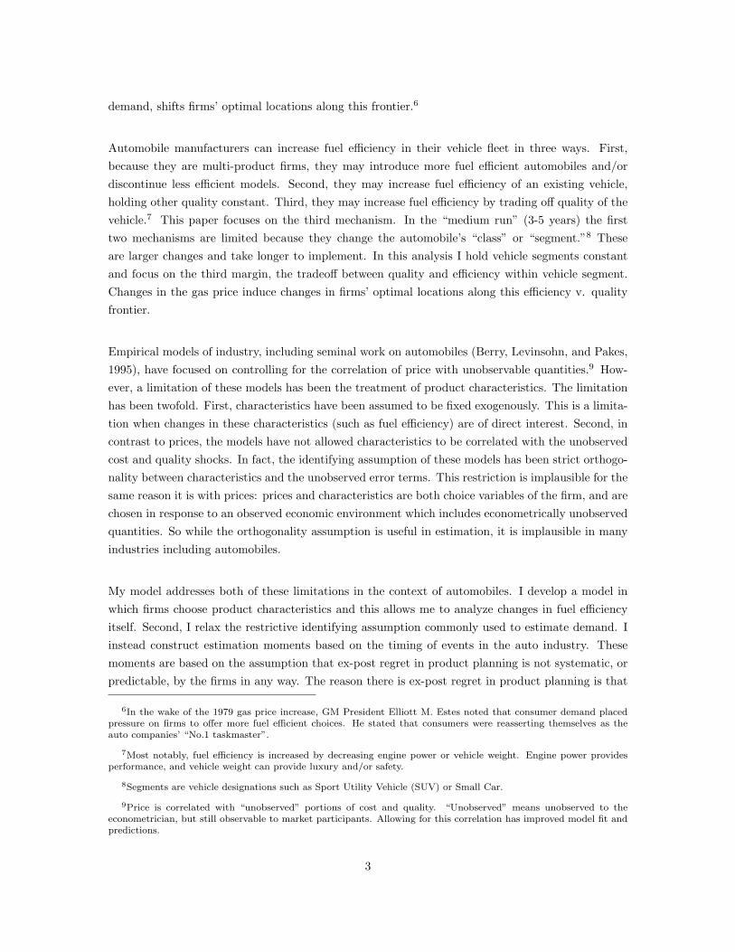
∂mpg , is increasing in the price of gas.18 The measure I use for qual is ln(mpg). Thismay seem counterintuitive to use the very quantity that trades off with quality to proxy for qualityitself. But it is a very strong empirical regularity that, conditional on both dpm and sub-segment,higher mpg is associated with lower “other quality” of a vehicle. This tradeoff can be pictured witha technology frontier for a given manufacturer within a given sub-segment, Figure 1 in the text. Iwill discuss first the concept of the frontier, then the suitability of ln(mpg) as a proxy for the qualityaxis.

14Any j subscript could itself be subscripted by t because model attributes change from year to year, but I suppressthis notation for ease of exposition. Where t subscripts do appear, they are to emphasize that some variables arecommon across all j in a given year (such as macroeconomic variables in Xjt) or to emphasize the frequency of someerrors or decisions (such as ε̃ijt).

15t would be the natural subscript for vehicle “type,” but it already subscripts time.

16Note the distinction between the technological parameter fuel efficiency (mpg) and the consumer preferenceparameter fuel economy (dpm).

17I do not separately model consumers’ vehicle utilization decisions.

18I.e., ∂2u∂mpg∂pgas

> 0.

6

Figure 1: Technology Frontier Within an Automobile Sub-Segment:

Technology Frontier

Fuel

Economy

Other Quality

This frontier reflects the tradeoffs (within a particular sub-segment) between providing efficiency andother attributes such as power (performance) and weight (luxury/safety). This tradeoff has beendocumented in previous work (Kleit, 1990). It is also evident in Figure 3 at the end of the text, whichshows the relationship between ln(mpg), ln(hp)19, and ln(weight) in my data. The tradeoff betweenln(mpg) and (these two) attributes of quality holds true at any level of vehicle aggregation, thoughfor purposes of my model it is important that it holds within a sub-segment (the lower right panelof the Figure). Table 4 shows this relationship in the form of a regression. ln(mpg) is regressed onln(hp), ln(weight), and a time trend to capture advancing technology. The regression shows a strongnegative relationship between fuel efficiency and both power and weight. The regression numbers inthe Table are pooled over all vehicle types, but at finer levels of aggregation the results change little.Despite the decreasing numbers of observations, the coefficients remain large and significant, andthe R-squared generally remains above .5. R-squared remains high despite decreasing numbers ofobservations because the technological relationship captured is increasingly precise.20 In my model

19hp is horsepower, a measure of engine power.

20The regression in Table 4 is of equilibrium choices of these three magnitudes by firms. Therefore, by itself theregression is not conclusive regarding the underlying production function. However, given the competitive structurein the automobile industry the relationship does suggest a tradeoff. Within an automotive sub-segment, firms cannot

7

I assume this tradeoff between fuel efficiency and other quality holds exactly within a sub-segment.

There are improvements that can be made to vehicle power and/or weight which sacrifice less fuelefficiency (or vice-versa). However, they are expensive and amount to changing the sub-segment ofthe vehicle. Luxury cars will have more horsepower than a mid-sized car with similar fuel efficiency,but it is much more expensive to produce the luxury car and it therefore does not compete in thesame sales segment. Another way to think of the technology tradeoff is that isocost curves exhibitthis shape, and competition within a sub-segment occurs along a single isocost curve. A firm can,to some extent, shift out the frontier, but only by incurring higher costs and switching segments ofthe market.

Independent of the question of whether technology tradeoffs exist, there is the question of whetherln(mpg) is an appropriate proxy for “other quality.” It seems counterintuitive because these wouldappear to be opposite axes of the same technology tradeoff. But there is reason to use ln(mpg) tocapture quality. The reason is that, conditional on dpm, ln(mpg) is the best empirical proxy for thequality tradeoffs. Any demand specification I estimate, no matter what observables are controlledfor, puts a negative and significant sign on ln(mpg) (provided dpm is controlled for). This meansthere are attributes of quality that are a) not measured in the dataset, and b) negatively correlatedwith ln(mpg). Trying to construct a metric for other quality based on all non-mpg observablesmisses some of these.21 One implication of this for future work is that specifications of automobiledemand ought to include both dpm and ln(mpg), not simply one nor the other. (At least until thedatasets are more rich).

As a final note on the subject, there is both conceptual and empirical reason to choose ln(mpg),rather than simply mpg or any other functional form, to represent “other quality.” Conceptually thequality tradeoffs required to move from 10 mpg to 20 mpg are larger than those required to movefrom 40 mpg to 50 mpg. The decreases in quality are decreasing in constant mpg improvements.Another way to think of this that increasing quality is more costly (in terms of efficiency sacrificed)as quality levels become higher. The second, empirical, reason to favor the logarithm is that itinsures the relationship between quality and efficiency always stays negative, whereas higher orderexpansions do not.22

push past the frontier without incurring extra costs and essentially changing the sub-segment within which the vehiclecompetes. If firms could attain more of both without a tradeoff, and/or without incurring costs, then the regressionrelationship would not hold.

21These unmeasured qualities likely include engine characteristics that can tweak mpg, conditional on power andweight. These may include timing of transmissions, gear ratios, turbo charging, cylinder shutdown, variable valvetiming, etc.

22The second order expansion bends back on itself around 55-60 mpg, and the third order expansion does reversethis because there is not enough data in that mpg range to calibrate it. So for high levels of mpg, increasing mpgimproves quality and this leads to non-sensible predictions in the counterfactual.

8

Given the above definitions, and with an additional linearity and separability assumption, consumerutility in Equation (1) becomes:

uijt = αpj + βddpmj + βmln(mpgj) + ξj +BXjt + ε̃ijt (2)

I expect α, βd, βm < 0. The nesting structure designations in Figure 2 come from Wards Automo-tive. The structure is a 3-level nest, where each level is an increasingly specific level of automobileclassification. The top level, vehicle type (v), are Cars, Utility Vehicles, and Trucks/Vans. The nextlevel, segment (s), consists of designations such as Small Car and Sport Utility Vehicle (SUV). Thethird and most specific level, sub-segment (ss) designates categories such as Lower Small Car, orLuxury SUV. Finally, the model (j) designate names such as Honda Accord or Ford Explorer.

The nested logit error term ε̃ contains parameters to be estimated (σss, σs, σv) which describe thesimilarity of choices within a nest. To be consistent with utility maximization, these nesting param-eters must be between 0 and 1 (Cardell, 1997). Appendix A contains details on the calculation ofnested logit shares and σ’s. The nested logit does restrict cross-price elasticities in a specific way.23

This means I do not measure substitution patterns as flexibly as if I were to forego the nesting struc-ture and include more utility covariates. As I will discuss in the supply side, however, the nestedlogit structure is instrumental in enabling my model of endogenous characteristic determination,and past empirical work in the auto industry has used the nested logit with some success (Goldberg,1995). So I find the tradeoff a reasonable price to pay.

Note that similar to other applied work, ξj from Equation (2) will be used in estimation moments.However, as I will also discuss in the supply section, I will use less restrictive assumptions on itsdistribution.

3.2 Supply

The timing of the supply side model is depicted in Figure 4 at the end of the text. One yearbefore the year of sale,24 firms observe gas prices, cost shocks, and demand shocks. In responsethey commit to product characteristics for each vehicle, still one year in advance, to allow for aproduction lag. Then, in the interim, gas prices change. Finally, in the year of sale, firms choose

23Choice probabilities within a nest, for the choices down one level, are logit based on inclusive value.

24As a robustness check I also estimate the model assuming 3 and 5 year lags in Section 7.

9

a price for each vehicle and consumers make purchase decisions. The information sets (H and I)as well as the ex-post regret (R) will play a role in the estimation moments as discussed in Section5. Note that this timing allow firms to observe their cost and demand shocks when choosing theirproduct characteristic, mpg, which is plausible but not allowed in previous models of the automobileindustry.

Firms take actions to maximize expected profit. Firms’ two choice variables (mpg and p) form asubgame-perfect Nash equilibrium. Each firm f ’s problem is:

maxmpgf

Epgas

[maxpf

Πf

](3)

Firm f ’s profits are given by:

Πf =∑j∈=f

Mtsj(mpg,p; θ) [pj −mcj(mpgj ; θ)− λft{bindft}(CAFEt −mpgft)] (4)

Subscript f is for firm, and recall that j is a model. =f is the set of cars produced by firm f ,as auto manufacturers are multiproduct firms. Mt is the size of the market (the number of U.S.households), sj is the market share of model j, and is a function of mpg and p, the entire industryvectors. θ is a vector of demand and cost parameters to be estimated. CAFEt are the stipulatedCAFE standards, and mpgft is the firm’s average fuel efficiency for determining CAFE compliance.25

{bindft} indicates whether the standards are binding for the firm, and λft is a firm and time-specificshadow cost of violating the standards. Recall that the t subscripts have been suppressed in a numberof places for ease of exposition.

Because of the Nash equilibrium assumption, derivatives of the profit function (with respect to thechoice variables) lead to first-order conditions of optimality. These hold with respect to the bothchoices, pj and mpgj , for each model j:

25CAFE standards calculate firm fuel efficiency as a harmonic average rather than a raw average. mpgf =qf∑

j∈=fqj

mpgj

. Harmonic averages are used to average rates, as they indicate the rate of fuel consumption when

all automobiles are driven the same distance. When averaging any (unequal) numbers, harmonic averages are me-chanically lower than raw averages, since low rates pull down more than high rates push up.

10

sj +∑r∈=f

[(pr −mcr)

∂sr∂pj

+ λ{bind}∂mpgf∂pj

]= 0 (5)

Epgas

∑r∈=f

[sr(

∂pr∂mpgj

− ∂mcr∂mpgj

) + (pr −mcr)∂sr

∂mpgj+ λ{bind}∂mpgf

∂mpgj

] = 0 (6)

Note that a single choice of mpg along the sub-segment frontier, or isocost curve, determines boththe fuel efficiency (dpmj = pgas,t

mpgj) and other quality (ln(mpgj)) for consumer demand. A challenge

in modeling product choice in any industry is finding exogenous variation to shift incentives to offercharacteristics. Characteristics-based models of auto demand have tended to include approximatelysix preference characteristics of automobiles. Because choices of these attributes are interrelated (forexample increasing fuel efficiency by decreasing engine power), a model that allows firms to chooseany of these characteristics must allow firms to choose them all.26 Having said this, however, it isdifficult to find instruments to shift firms incentives’ to provide all six characteristics in the autoindustry. Some industries have the benefit of having many local, geographic markets in the crosssection that provide variation in market structure (e.g. Lustig (2008)) to shift incentives. However,automobile supply is one, national market each year, so any shifter must have national time-seriesvariation.

My solution to this problem is to use the nested logit structure, the technology tradeoff, and anassumption of medium run time horizons. First, the nested logit structure captures consumer sub-stitution patterns without having to use a full set of characteristic controls. Consumers in my modelare free to have preferences over other/all auto characteristics, but I do assume these preferencesinfluence the sub-segment choice itself, not the choice within sub-segment. The choice within sub-segment is based only on two non-price characteristics (econ and qual).27 Having used the nests toreduce the endogenous choices to two, I use the technology tradeoff to parameterize these two choicesinto one choice. Third, I restrict firms from changing the sub-segment of their vehicles. This essen-tially amounts to assuming a medium run horizon of perhaps 5 years. Changing the sub-segment ofa car essentially means rebranding and reintroducing, and this is likely to be difficult to do in under4-5 years.28 So these three modeling features - the nesting structure, the technology tradeoff, andthe medium run focus - allow me to pare down the endogenous choice variables to a single choicempg (which determines the two utility characteristics), and there is a clear stochastic and exogenous

26Allowing firms to choose only some characteristics, while treating others as exogenous, would bias measuredincentives.

27Which is more general than saying that competition throughout all vehicles is only based on these two character-istics.

28On the other hand, modifying an engine to gain/lose fuel efficiency is something that can, and does, happen morefrequently.

11

shifter for this characteristic choice is the gas price.

There are costs of this approach. Though the nested logit captures some relevant consumer behavior,there is likely loss of richness in the demand system by not retaining more preference characteristics.Also, because I limit my attention to the medium run, there are interesting longer-run decisions anddynamics which I will not capture in the model. I find think these costs are worth the price to pay forbeing able to model fuel efficiency choice. Nested logits work better when the more nesting groupsare relevant to consumers’ decisions, and there is some indication in the trade press and previousempirical literate29 that this is at least somewhat true with autos. In terms of the medium-runrestriction of the analysis, this is at least an improvement on previous work which was unable toanalyze fuel efficiency choice on any time horizon. I trust that future work will develop methods tolook at issues of new model introduction.

Firms face constant marginal costs of producing automobile j:

ln(mcj) = mc(mpgj , Xjt, ωj , t) (7)

The specific functional form I use is:

ln(mcj) =γ1 + γ2ln(mpg) + ΓXjt + ωj (8)

Because firms locate along an isocost curve, the standard interpretations of γ2 does not necessarilyapply. Normally in empirical work a term like γ2 is expected to be greater than zero because it isattached to a good. But here, ln(mpg) is a parameterization of a tradeoff between 2 goods, ratherthan a good itself. Within a sub-segment, cars with relatively more fuel efficiency may or may notbe more expensive to produce. In fact, the better the model approximation of reality, the morelikely that γ2 = 0. The model does not impose this restriction, but it is an implication check of themodel.30 X is a full set of sub-segment dummies, country of origin, and a time trend. ωj is theunobserved product cost (unobserved but inferred from the data).

Note that ωj , like ξj in demand, are used in estimation moments. However ωj , also like ξj , is usedin a less restrictive way than in previous work.

29Goldberg (1995) and Goldberg (1998).

30If my proxies for economy and quality closely match consumer valuations, and competition within the sub-segmentis nearly on a single-isocost curve, then γ2 should estimate out to 0.

12

3.3 Modeling CAFE Standards

The federal government’s fines for violating CAFE standards in a given year are $55 per car soldper 1 mpg below the standard that the firm average falls. It is commonly thought, however, thatthere may be additional reputation and political costs to American manufacturers of violating CAFEstandards. The Big Three31 have influence over the CAFE standards through their relationship withthe federal government. One thought is that these manufacturers may risk this influence by violatingthe standards, or might lose reputation with American consumers by violating our country’s owndomestic energy policy. I leave the fine (λ in Equations (5) and (6)) as a shadow cost to be estimated.The estimation results can thus speak to whether the implicit costs are higher than the fine alone.

For simplicity, I assume CAFE binds on all American manufacturers in all years after 1977, and onno other manufacturers in any years. This is not exactly true, but is a reasonable approximation ofboth a somewhat complicated system of carry-overs and credits used in calculating CAFE fines, andhistorical evidence on sales-weighted fuel efficiency. For Asian manufacturers, CAFE has not bound.They have never paid fines, and have never been particularly close to the standards. Some Europeanfirms have paid $55 per car-mpg fines. (In fact, European firms are the only firms to have ever paidCAFE fines.) However, for these European firms there is likely less political pressure to abide byU.S. domestic energy policy than there is for U.S. firms. These fines to European manufacturershave tended to be on small fleets of luxury and sports cars where the pecuniary penalties are a smallportion of the list price. I simply add them as an extra tax to these models, rather than estimate ashadow cost of compliance. American firms, in contrast to both Asians and Europeans, are likely tohave been genuinely constrained over the years. They face unique pressure in being the domestics,and they have hovered close to the regulation for many, many years. No American manufacturerhas ever actually paid a fine, but this is only due to the system of carry-overs and credits from yearto year. The standard looks to have been binding or near binding for the whole time period since1977 when the standards began. The model is general enough to handle a rich set of year-specific,firm-specific shadow costs, but I estimate only one shadow cost. Interpreting yearly costs wouldbe muddy because of the system of carryovers, and each shadow cost is an extra non-linear searchparameter for the GMM search routine. So for computational reasons fewer terms is preferable. Isimply assume one shadow cost on all 3 American manufacturers, starting in 1977.

31General Motors, Ford, and Chrysler are the three American manufacturers.

13

4 Data & Industry

The model is estimated using data on all new automobiles sold in the U.S., and macroeconomicdata, from 1971-2007. I have data on all sales and characteristics of passenger vehicles during thattime period with two exceptions. First, I’m missing data from 1991-1995. The collection of theearlier data stopped in 1990, and the electronic data-keeping by Wards Automotive did not beginuntil 1996. Second, I’m missing truck data for the early years (1971-1990), which were not collectedwith the original data set.32

The early year data, 1971-1990, are the same data used in Berry, Levinsohn, and Pakes (1995), andwere generously shared with me by the authors. These data are from Automotive News Market DataBook, and contain information on sales and base model characteristics of all passenger cars sold inthe U.S. I supplement these with segment information that I collected from Wards Automotive Year-books. The later data, 1996-2007, are from Wards Automotive. They contain sales, characteristics,and segment data on all passenger vehicles sold in the U.S. during those years. Table 5 in the backof the text shows popular cars in the various sub-segments for the later years.

Prices are list prices, fuel efficiency is city fuel efficiency as measured by the EPA (U.S. EnvironmentalProtection Agency). The unit of observation is the vehicle model, the level at which sales data arereported. I use the characteristics of the base model for each model-year.33

I also collect macroeconomic data from various government agencies: the Energy Information Ad-ministration (gas prices), Bureau of Labor Statistics (CPI, number of households, unemployment,income distribution), and the Bureau of Economic Analysis (GDP and GDP growth).

Table 6 contains selected summary statistics from all data sources. Sample average mpg is 20.7.(At a finer level of detail this would be higher for Cars and lower for Trucks and Utility Vehicles.)There is substantial variation in the gas price, both in levels and in changes. Note that year-to-datethrough August 2008 (outside the sample summarized in the Table) the gas price jumped from $2.80to $3.43, which is above the highest real gas price of the sample. This jump also nearly equalledthe highest change of the sample, which is $0.68 in 1980. The summer of 2008 is analyzed in thecounterfactual Section (8). There are 4,820 model-years over the course of 32 years, for an averageof 151 models offered each year. There are 3 vehicle types, 9 vehicle segments, and 28 vehiclesub-segments.

32I intend the collect the missing years of data to supplement the analysis.

33Models have even finer distinctions of various trim levels. These offer slightly different configurations of enginesand accessories. I ignore this in my analysis, as I do not have sales data at this level. The base model is usually themost fuel efficient trim of each model.

14

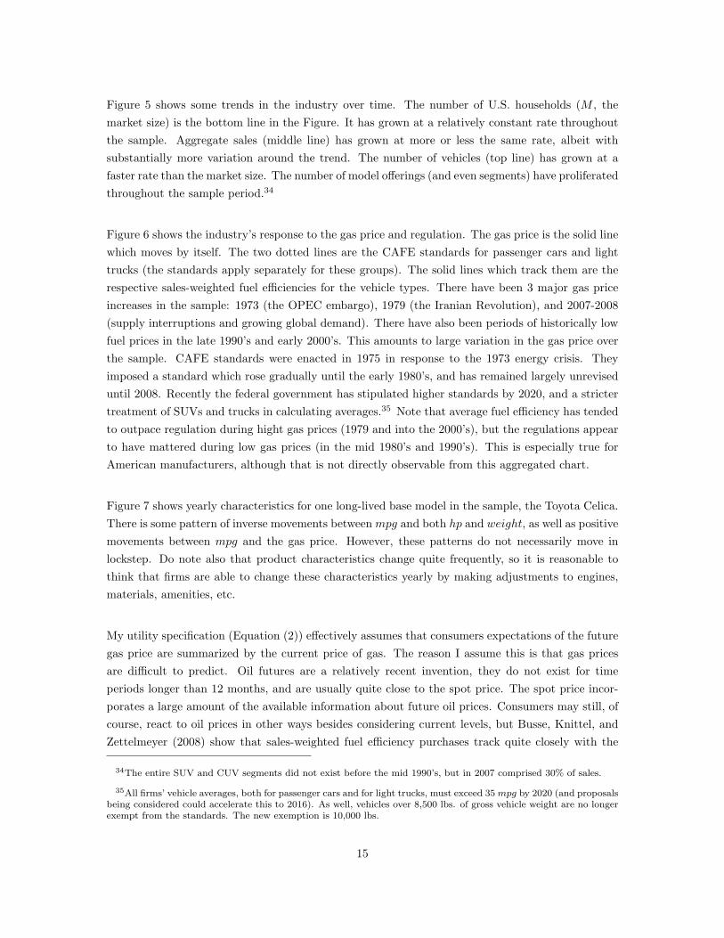
Figure 5 shows some trends in the industry over time. The number of U.S. households (M , themarket size) is the bottom line in the Figure. It has grown at a relatively constant rate throughoutthe sample. Aggregate sales (middle line) has grown at more or less the same rate, albeit withsubstantially more variation around the trend. The number of vehicles (top line) has grown at afaster rate than the market size. The number of model offerings (and even segments) have proliferatedthroughout the sample period.34

Figure 6 shows the industry’s response to the gas price and regulation. The gas price is the solid linewhich moves by itself. The two dotted lines are the CAFE standards for passenger cars and lighttrucks (the standards apply separately for these groups). The solid lines which track them are therespective sales-weighted fuel efficiencies for the vehicle types. There have been 3 major gas priceincreases in the sample: 1973 (the OPEC embargo), 1979 (the Iranian Revolution), and 2007-2008(supply interruptions and growing global demand). There have also been periods of historically lowfuel prices in the late 1990’s and early 2000’s. This amounts to large variation in the gas price overthe sample. CAFE standards were enacted in 1975 in response to the 1973 energy crisis. Theyimposed a standard which rose gradually until the early 1980’s, and has remained largely unreviseduntil 2008. Recently the federal government has stipulated higher standards by 2020, and a strictertreatment of SUVs and trucks in calculating averages.35 Note that average fuel efficiency has tendedto outpace regulation during hight gas prices (1979 and into the 2000’s), but the regulations appearto have mattered during low gas prices (in the mid 1980’s and 1990’s). This is especially true forAmerican manufacturers, although that is not directly observable from this aggregated chart.

Figure 7 shows yearly characteristics for one long-lived base model in the sample, the Toyota Celica.There is some pattern of inverse movements between mpg and both hp and weight, as well as positivemovements between mpg and the gas price. However, these patterns do not necessarily move inlockstep. Do note also that product characteristics change quite frequently, so it is reasonable tothink that firms are able to change these characteristics yearly by making adjustments to engines,materials, amenities, etc.

My utility specification (Equation (2)) effectively assumes that consumers expectations of the futuregas price are summarized by the current price of gas. The reason I assume this is that gas pricesare difficult to predict. Oil futures are a relatively recent invention, they do not exist for timeperiods longer than 12 months, and are usually quite close to the spot price. The spot price incor-porates a large amount of the available information about future oil prices. Consumers may still, ofcourse, react to oil prices in other ways besides considering current levels, but Busse, Knittel, andZettelmeyer (2008) show that sales-weighted fuel efficiency purchases track quite closely with the

34The entire SUV and CUV segments did not exist before the mid 1990’s, but in 2007 comprised 30% of sales.

35All firms’ vehicle averages, both for passenger cars and for light trucks, must exceed 35 mpg by 2020 (and proposalsbeing considered could accelerate this to 2016). As well, vehicles over 8,500 lbs. of gross vehicle weight are no longerexempt from the standards. The new exemption is 10,000 lbs.

15

current gas price, not outpacing it nor lagging it. So this is the specification I use in the estimationresults, and I discuss other specifications in the robustness Section (7).

5 Estimation

The estimation routine is Generalized Method of Moments, and the moments are constructed fromthe timing of the model.

5.1 Estimation Moments I

To help understand the estimation moments, it is useful to refer again to Figure 4, the model timing.The two information sets defined in the Figure are snapshots of information at various points in theyear leading up to production. These information sets, when they are visible, are visible to allmarket participants. Loosely speaking, these sets are:

Ht−1 = {Information known about time t at the “beginning” of time t− 1} (9)

It−1 = {Information known about time t at the “end” of time t− 1} (10)

Take the example year t=2008. Let Ht−1 be the knowledge at the beginning of 2007, before 2008characteristics are chosen, about what the auto industry will look like in 2008. This includes the setof all 2008 models, their manufacturers, their sub-segments, and the 2007 gas price. Ht−1 does notinclude the cost and demand shocks, mpg choices, or gas prices and macroeconomic variables thatwill prevail in the 2008 marketplace.

Then, still in 2007, the cost and demand shocks, ω and ξ, that will affect the 2008 market are revealedto all manufacturers on all models. They are common knowledge. In response to these, and still in2007, mpg is chosen for all 2008 models. Now take another snapshot and redefine this informationset as It−1. It contains Ht−1, but is also updated to include shocks and mpg. It still, however, doesnot include the final pieces of the 2008 market - gas prices and macroeconomic variables. So, morespecifically:

16

Ht−1 = {1, pgas,t−1, ownership/sub-segment of year t models} (11)

It−1 = {1, pgas,t−1, ownership/sub-segment of year t models, ωt, ξt,mpgt} (12)

ωt, ξt, and mpgt are vectors for the entire industry, observed by all participants. The inclusion of“1” in these information sets simply indicates that anything (shocks or ex-post regret) orthogonalto these information sets should be mean zero.

Two estimation moments that are implications of this timing (rather than new assumptions), arethat demand and cost shocks are uncorrelated with Ht−1:

E[ξjt ∗Ht−1] = 0 (13)

E[ωjt ∗Ht−1] = 0 (14)

These moments hold model by model - no vehicles’ demand or cost errors should be correlated withthe exogenous observables. Errors are always orthogonal to observables in empirical work - the logicof this assumption is standard. However the formulation here is less restrictive because I exclude theendogenous choice variable mpg from the instrument set. This means that in my model firms areable to observe market shocks when choosing their mpg, and this allows for a free correlation betweenerrors and mpg. The standard demand identifying assumption would be to add mpgt into what Icall Ht−1, which would mean firms are unaware of the cost and demands shocks when they committo characteristic decisions. This scenario is implausible in the auto industry because automobilemodels survive multiple years and there is learning. For example, the Toyota Camry sells quite wellrelative to other cars with comparable characteristics. This indicates a high ξ for the Camry, andall auto firms are likely to be aware of this when they choose their own product characteristics.36

36In addition to observing the shocks, firms might actually be choosing these shocks, or at least a portion of them.In the automotive industry, firms likely choose a portion of these shocks. I do not allow for this in my model,however, because doing so would require additional assumptions in order to split a single unobservable quantity intotwo unobservable portions (chosen and unchosen), and/or additional exogenous variation as an instrument. This isan interesting pursuit for future work.

17

5.2 Estimation Moments II

The second set of estimation moments are, like the first set, implications of the timing of the modelrather than new assumptions. They are the first-order conditions on optimal firm choice of p andmpg in (see Equations (5) and (6)). Because the first-order condition for mpg has an expectation, theempirical counterpart will not hold exactly equal to zero. I have two choices as to how to handle thewedge. One is that I can simulate the empirical distribution of gas price change to approximate theintegral in the expectation, and make this integral hold equal zero. Because this is computationallyburdensome, and requires me to commit to my belief as to firms’ beliefs concerning gas prices, Iinstead use a second method outlined in Hansen and Singleton (1982).

To understand the Hansen and Singleton moments, define:

Rjt =∂Πft

∂mpgjt(15)

Rjt =∑r∈=f

[(pr −mcr)

∂sr∂mj

+ sj(∂pr∂mj

− ∂mcr∂mj

+ λ{bind}∂mpgf∂mj

)]

(16)

Rjt is the derivative of the profit function with respect to mpgjt. It is the ex-post regret in mpg

choice. In Figure 4, this appears at the extreme right of the timetable. It is the object which is setto zero in expectation in the firms’ first-order condition. But because the gas price changes aftermpgjt is chosen, Rjt will not generally equal zero in the year of sale. It represents the ex-post regret(thus the choice of the letter R) in the mpgjt choice. Another way of saying this is that if firmscould readjust mpgjt during the year of sale, they would. This is not the same as saying that firmsfail to optimize. Firms do optimize, they simply must do so at a time when not all the informationthey would wish to see (the gas price) has been revealed.

With this definition, Hansen and Singleton (1982) note that an implication of stochastic optimizationis:

E[Rjt ∗ It−1] = 0 (17)

This says there are no patterns of ex-post regret (Rjt) which are systematic, or in any way predictableat time t−1. If there were such patterns, then this would, indeed, imply that firms are not optimizingcorrectly. That would be inconsistent with the model.

The benefit of this estimation approach is twofold. First, it is far less computationally burdensomethan simulating the empirical distribution of gas price changes. Second, it allows me to remain

18

agnostic about firms’ beliefs as to future gas prices.

As I have mentioned, I do experiment in the robustness section with placing It−3 and It−5 intoEquation (17) to reflect the possibility that firms have to choose product characteristics more than1 year before the year of sale. Note that all that is different in these two information sets is that theolder gas prices (pgas,t−3 and pgas,t−5, as opposed to pgas,t−1). I discuss the results of this robustnesstest further in Section 7.

5.3 Estimation Mechanics

Three moments, (13), (14) and (17) are stacked for estimation. The fourth equation, the pricing first-order condition (in Equation (5)), holds exactly for any parameter values because of the continuousfunctions ξ(θ) and ω(θ) (Berry, 1994). So that equation does not enter estimation as a moment,though it is used within each moment evaluation to back out the error terms. Estimation is by2-stage GMM (Generalized Method of Moments). Parameter values are chosen to minimize thefollowing objective function:

minθ

ξt(θ) ∗Ht−1

ωt(θ) ∗Ht−1

Rjt(θ) ∗ It−1(θ)

Wn

ξt(θ) ∗Ht−1

ωt(θ) ∗Ht−1

Rjt(θ) ∗ It−1(θ)

′

(18)

There are only 4 parameters that require non-linear search - the three nesting parameters (σ’s in theutility function), and the shadow cost on CAFE compliance (λ). Conditional on these 4 parameters,the rest of the parameters in θ can be calculated by Two Stage Least Squares to minimize the valueof the moments. I choose starting values for the 3 nesting parameters based on Two Stage LeastSquares estimates of demand with just the first two moments. I choose starting values for the CAFEstandard based on the pecuniary fine $55, though the search routine is not sensitive to any of thesestarting values.37

In the first stage of GMM, Wn is a block diagonal matrix containing the inverse of the normalizedinstrument matrices Ht−1, Ht−1, and It−1(θ). The only non-standard part of the routine is thatweight matrix is updated for each parameter guess, because It−1 is a function of θ by virtue of con-taining the elements ξ(θ) and ω(θ). In the second stage of GMM, Wn is the standard block diagonalmatrix containing the inverses of the variance-covariance matrices of the moments themselves.

37The objective function has a clear global minimum, which the estimation finds.

19

I do ignore two equilibrium effects in the calculation of Rjt (Equation (16)) because they are likelyto be small in magnitude and yet add considerable computational complexity. The first is the∂p

∂mpgjterm - the effect that changing one’s fuel efficiency will have on the equilibrium prices (of

all vehicles) played in the subsequent game. I assume this term to be zero. The second omissionis that in calculating ∂mpgf

∂mj, I ignore ∂q

∂mpgj- the effect that changing one’s fuel efficiency will

have on equilibrium quantities in the downstream game.38 In sum, I ignore effects of mpg choiceson the equilibrium of the downstream pricing and purchasing game. This means that I am onlyapproximating the subgame perfect Nash equilibrium, but this approximation is a reasonable priceto pay for tractability. These terms are likely to be small because of the number of automobiles inthe market is large.

6 Estimation Results

The results of the GMM estimation are reported in Table 7. They exhibit sensible and statisticallysignificant parameter estimates. The nesting parameters (σ’s) are between one and zero. α, βd,and βm, are significant and negative as expected.39 There are three findings that are of particularinterest: the shadow cost of the CAFE standards, the “cost” of providing fuel efficiency, and theresults for fuel efficiency preference by segment.

First, the parameter estimate on the CAFE standard indicates that the shadow cost to Americanmanufacturers of violating the CAFE standards is $347 per vehicle per year. This is significantlylarger than the non-compliance fine of $55 per vehicle per mpg. A common hypothesis is that theseshadow costs are due to political and reputation pressure, either from the federal government and/ordomestic consumers. Whatever the cause, the parameter estimates are consistent with the notionthat American manufacturers incur lost profits due to the regulations. This also suggests that duringthis time period domestic manufacturers would have set lower fuel efficiency in the absence of theCAFE standards. American manufacturers did not actually pay any fines during this time period -the shadow cost estimate is rather an indication that they incurred significant resources trying notto.

The second result of interest is the coefficient on ln(mpg) in cost. It is not insignificant. This resultwas not imposed by the model, but rather is an implicit test of model specification that turns outfavorably. Unlike most empirical cost functions, when firms provide more mpg they also provide lessquality. They slide along a production frontier, or isocost curve, for the given sub-segment, rather

38This term also includes another instance of the first ignored term, ∂p∂mpgj

.

39Recall that higher dpm means less fuel economy, higher ln(mpg) means less “other quality,” and p always entersutility negatively.

20

than incurring more cost to provide more mpg ceteris paribus. The sub-segment dummies do thelion’s share of the work on the cost side, not surprising given that competition within sub-segmentsis along an isocost curve.

The third result of interest is the set of findings concerning preference for fuel economy. Preferencefor fuel economy (dpm) is allowed to vary by segment. Note that all segments have a preference forfuel economy (all 9 coefficients are negative), but some moreso others. Conditional on sub-segmentof purchase, Utility Vehicle purchasers are actually the most sensitive to fuel economy. Luxury Carand Van purchasers are the least sensitive to fuel economy. Trucks, and the remaining four carsegments are in between.

It may seem counterintuitive that purchasers of Utility Vehicles (Crossover Utility Vehicles, CUVs,and Sport Utility Vehicles, SUVs) are the most conscious of fuel efficiency, because these vehicles(especially SUVs) are rather fuel inefficient. However, it is actually a sensible result, given thatit is conditional on sub-segment purchased. A driver saves more money by increasing mpg on agas-guzzler than on an efficient vehicle. Adding 2 mpg to the mean SUV (16.2 mpg in 2007) savesmore gas money than adding 2 mpg to the mean middle sized car (28.2 mpg in 2007), conditionalon equal mileage driven by each car.40 Despite, and perhaps even because of, UVs being inefficientcompared to other segments, competition within the segment is quite sensitive to fuel efficiency.Another way to interpret the result is that drivers have chosen this segment for reasons other thanefficiency (they may need the space, or prefer the safety or amenities of an SUV), but once in thesegment the returns to fuel efficiency are high.41 In the summer of 2008 when gas prices were quitehigh, the market saw large declines in SUV purchases relative to other segments. This corroborates,rather than refutes, the notion that UV purchases are efficiency-minded.

I put a time trend on CUV and SUV utility. This is not standard - generally the literature assumespreferences are stable over time. One of the virtues of a hedonic demand system is that it cantease out a stable set of preferences despite large product turnover. However, there is a historicalcoincidence that makes a time trend on these segments necessary, in my judgement. That coincidenceis that the two UV segments were introduced in the mid 1990’s, and grew steadily and rapidly in sales(0 to 30% market share within 10 years) at the same time that the gas price was also steadily andmonotonically rising. With no time trend in the model, the estimation attributes this correlationto consumers of these vehicles having a strong dislike for fuel economy. I think it is more likelythe case that utility for these vehicles was growing because consumers were gaining experience andfamiliarity with the vehicles. So I have chosen to add a time trend to utility to capture experienceand familiarity. This restores the natural result that consumers prefer lower gas expenditure, not

40This is the reason many countries express fuel efficiency as Volume per Distance rather than Distance per Volume:fuel costs are linear in Vol/Dist, but concave in Dist/Vol. Some have argued that we ought to adapt the same systemin the United States(Larrick and Soll, 2008).

41 ∂2u∂mpg∂mpg

< 0.

21

higher.

To interpret the magnitudes of these parameter estimates, I have calculated willingness-to-pay(WTP) for fuel efficiency increases in Table 8. WTP depends on a number of factors: segment,starting mpg, ending mpg, and the price of gas.42 Concerning segments, I display all 9. Concerningstarting and ending mpg, I consider a 20% improvement from the segment-average mpg. Becausethe segment averages are different, this means that both the starting mpg, and the absolute mpgimprovement, are different across segments. This is still the fairest comparison, because the alter-native is to compare a single mpg jump (such as 20 to 24 mpg) across all segments. But any singlejump means very different things across segments. Lastly, concerning gas prices, I choose three gasprices at which to display WTP. These are $1.50, $3.43, and $4.55. $1.50 is a relatively low gasprice, $3.43 was the price from the summer of 2008, and $4.55 is the gas price we’d need to achieve35 mpg as an industry. ($3.43 and $4.50 are the two prices that I feature in the section on policyimplications (Section 8)).

As anticipated by the unequal segment preferences for dpm, there are unequal segment WTP formpg. Within a segment, higher gas price always means higher willingness to pay. At $3.43 gas, SUVconsumers are willing to pay $7,059 for the 20%-from-average mpg improvement. CUV consumers$5,246. Luxury car purchasers were almost indifferent to fuel efficiency at average levels, and mostsegments’ consumers were willing to pay between $1,000 - $3,000 for the 20% increase.

Note that for low gas prices WTP for higher fuel efficiency can be negative. This is because ofthe quality tradeoffs associated with higher efficiency. At a high enough gas price, all WTPs arepositive, and at a low enough gas price all WTPs are negative. Table 9 shows, for comparison, thewillingness to pay for efficiency improvement without quality loss. This Table does not reflect howthe model works, nor how I believe the real industry works, but I include it for comparison. Withoutquality adjustment, all WTPs are both a) higher than their quality-adjusted counterparts, and b)necessarily higher than 0.

GDP variables are statistically significant, especially GDP growth per capita. “autonews” is adummy indicating the variable is from the early years of the data when Truck/Van data are notcollected. Therefore vehicles (cars) from this time period are deemed to have a higher intercept.Costs are increasing over time, and are higher for Asian and European vehicles.

The model implies a mean Lerner index ((p-mc)/p) of 32.5%, and a minimum of 3.9%.

42WTP is higher during times of high gas price because the marginal benefit of fuel efficiency, ∂u∂mpgj

, is increasing

in the price of gas. ∂2u∂mpg∂pgas

> 0.

22

Table 1: Estimated Correlation of Shocks and Characteristics

mpg p ωξ -0.28 0.45 0.25ω -0.26 0.61

Allowing for correlation between errors and characteristics proves to have quantitative significance.The correlations are reported in Table 1, in the text. Previous literature had allowed for the corre-lation with price (second column), but not the correlation with characteristics (first column). Thenew correlations are not as large as the existing correlations, but this is unsurprising. All qualityis priced to the consumer, but not all quality correlates with all other dimensions of quality. Carswith high demand and/or cost errors tend to be of the less efficient - more quality variety.

7 Robustness

There are a number of robustness checks of the model that I run. First, one might assume thatfirms set product characteristics before year t − 1. In other words, there may be a longer leadtime in production than 1 year. I have tested this alternative assumption by assuming productcharacteristics are set 3 and 5 years from the year of sale. This changes the estimation resultssurprisingly little. Though the change is large conceptually, mathematically all it means is that asingle element of the instrument set (pgas) is changed. Furthermore, the 3 and 5 year lagged gasprice is (serially) correlated with the 1 year lag, so the instrument set is largely unchanged. This is astrength of the model - that it is fairly robust to when, exactly, firms must lock in their productiondecisions.

A second robustness check is whether the addition of the sub-segment level of the nest is too fine apartition for automobiles. When nesting groups are too finely partitioned, too much of the utility canend up being generated by the nest shares. This can lead to minimal substitution across nests. I re-estimate the model omitting sub-segments, but the results also change little. The nesting parametersare still relatively high. Substitution patterns in the counterfactuals are plausible with the 3-levelsof nest, so I prefer this specification as it adds more richness to the demand specification.

A third robustness check is to incorporate consumers who are forward (or backward) looking withrespect to the price of gas. This is done with interactions of fuel efficiency preference and lagged gasprices and/or movements. Upswings could, for example, make people more aware of gas prices andthus more sensitive to fuel efficiency. On the other hand, upswings could make people less sensitiveto fuel efficiency if they expect prices to mean revert. It turns out that in this sample the formeris somewhat true, though the effect is not large and steals some statistical precision from the dpm

23

term itself. Therefore I prefer the specification with only the spot price of gas (as the numerator ofdpm). Other work has documented that consumers’ preferences for fuel efficiency follows the spotprice of gasoline rather closely (Busse, Knittel, and Zettelmeyer, 2008).

I have also experimented with other controls (in X) on both demand and cost. I left out mostwhich were insignificant. These included other functional forms of mpg, interaction terms with mpgand gas prices, and macroeconomic variables attempting to further control for the utility of theoutside good (such as the Federal Funds Rate, unemployment, and election year dummies). Thefinal specification leaves in the terms with explanatory power.

8 Counterfactuals: Summer 2008, and 35 mpg

8.1 Introduction

Having developed a model in which firms are free to choose the fuel efficiency of their new vehicles,I now use the model to learn about how the market would respond to various gasoline prices andtaxes. Higher gasoline prices lead to a higher consumer sensitivity to fuel efficiency, and this in turnyields incentives for firms to raise fuel efficiency in their vehicles even though it requires makingquality tradeoffs. As we consider ways to curtail energy expenditure and pollution, one option isgasoline taxes. Gasoline taxes raise the price of gasoline that consumers pay. Consumers wouldtherefore want fuel efficient cars, and firms would have incentive to offer them.

There are other policy instruments that raise fuel efficiency - most notably the CAFE standards.The CAFE standards stipulate minimum sales-weighted fuel efficiency, firm by firm, and levy finesfor non-compliance. The United States has had the CAFE standards in place since 1975, and thereis evidence these have affected the fuel efficiency of new vehicle purchases. However, there havealso been criticisms of the CAFE standards both in the academic literature and in the press.43

Some criticisms apply equally to any policy that would increase fuel efficiency - for example thatthey encourage smaller cars which are less safe. Other criticisms of CAFE apply specifically vis-a-vis gasoline taxes. These criticisms have a common theme - that because the Standards do nottarget the specific behavior that causes the negative environmental externality (burning a gallon ofgasoline), they have perverse effects and do not achieve their intended ends. One example is thatboth trucks and heavy vehicles receive more lenient Standards. This gives perverse incentive toproduce more of these inefficient vehicles. Another example is that while the Standards may affect

43Gruenspecht (1982), Crandall and Graham (1989), and the series of citations herein by Kleit are some of themany academic papers which discuss the CAFE standards.

24

Table 2: International Gasoline Taxes

Average Gas Taxes Per Gallon

August 2006

U.S. taxes include all State and Federal Taxes

Source: International Energy Agency (IEA), "Energy Prices and Taxes"

As reported in NYT, "Raise the Gasoline Tax?" Oct 2006

$4.24

$3.99

$3.80

$3.75

$2.07

$1.03

$0.40

$- $1.00 $2.00 $3.00 $4.00 $5.00

Britain

Germany

France

Italy

Japan

Canada

U.S.

new vehicle purchases, they do not necessarily curb driving (the gas-burning) behavior. In fact, theeffect on driving could be perverse: shifting people into more fuel efficient cars, while gas prices arestill relatively low, could induce more driving. Taxing gasoline, on the other hand, would attachthe policy instrument directly to the externality causing behavior of driving. This would solve bothof the above problems. Some argue, therefore, that taxes are a more effective (less costly) way toachieve any given level of fuel conservation.

There is international precedent for using gasoline taxes, either in addition to or instead of regulationsuch as CAFE. Consumers in many industrialized nations face considerably higher gasoline taxesthan the United States. (See Table 2 set in the text.) Many of these nations also have considerablyhigher fuel efficiency than the United States. The European Union sees over 40 sales-weighted mpg,compared to the United States which is under 25. This correlation does not establish causation, andthere are many factors which affect nations’ fuel efficiency.44 However, the link between gasolinetaxes and fuel efficiency in noteworthy, and gives context to our own consideration of domesticgasoline taxes. Higher gasoline taxes in European countries mean these consumers routinely pay$6-$8 per gallon of gasoline, and even more during global oil price spikes such as in the summer of2008.

This section will consider two policy scenarios in this country. First, what would happen to domestic

44Some of these nations even have regulations similar to the CAFE standards (ICCT, 2007).

25

Table 3: Actual and Predicted Sales Declines, Summer 2008

Aggregation Level Actual Model PredictionCars -3% -9%Utility Vehicles -19% -23%Trucks -16% -13%Total -13% -14%

fuel efficiency if the gas price were $3.43? Second, what would the gas price need to be in order toachieve 35 mpg industry wide? The first scenario is of interest because this was the summer 2008gasoline price when consumers because to react dramatically. During summer months the price waseven higher than $3.43, but $3.43 was the annualized average price through August so I can compareYTD sales with model predictions. The second question of 35 mpg is of interest because recent policyproposals have stated a goal of raising the CAFE standards to 35 mpg by 2016. To preview theresults of both scenarios, the $3.43 gasoline (a 23% price increase over 2007) would increase averagefuel efficiency offered to 26.9 mpg (a 31% increase) and sales-weighted fuel efficiency to 26.4 mpg

(a 17% increase). The level of gas price (after tax) that would be require to boost market-wideefficiency to 35 mpg would be $4.55 per gallon.

8.2 What Happens at $3.43 Gasoline?

When the price of gasoline rose quickly to $3.43, as it did in the summer of 2008, the first responseis from consumers. Firms do not have a chance to adjust their product lines in the middle of theyear, but consumers can adjust their purchasing behavior overnight. In the summer of 2008, the didso. All car sales were down, but even moreso in the SUV and truck segments as compared to cars.Table 3 in the text reports actual and model-predicted sales declines for August year-to-date 2008automobile sales. The predictions at the finer aggregations levels are somewhat less precise, but thegeneral shape/ordering of these predictions matches well, as does the overall level.

Table 3 is a condensed version of a table at the back of the text, Table 10. That Table tells thecomplete story of the counterfactual. The counterfactual can be thought of in three stages. First,2007 is used as a baseline before the gas price increase. Then, 2008 is the year of the gas priceincrease - consumers have time to respond but firms do not. Then, in 2009, firms have the chanceto update their characteristics. The 2009 column represents the new equilibrium of mpg offeringsand purchases under $3.43 gasoline.

A few notes are in order about this new equilibrium. First, because gas prices fell back downtowards the end of 2008, it is not realistic to expect these “2009” fuel efficiency improvements tohave materialized in 2009. These are simply what the model predicts would have happened if high

26

gas prices had remained long enough to be reflected in new model years.

Second, despite calling this the “2009” equilibrium, I prefer to remain agnostic as to exactly how/howquickly would firms would arrive at this equilibrium, and whether or not it would be within a year.I have been able, in the model and in estimation, to remain rather agnostic about production lags.This is a strength in the model, though it means less specificity in the timing of the counterfactual.This tradeoff is reasonable, because I believe the level of the new equilibrium to be more interestingthan the timing of the adjustment path to arrive there. Gas prices and product planning areadmittedly much more continuous processes than the once-a-year snapshot of data that I observe,so trying to overextending the model’s ability to predict timing would add little value. Firms mayadjust more quickly or slowly based on when (in the model planning year) information about gasprices is revealed, whether a policy was pre-announced, and depending on production lead times.But the model indicates that at $3.43 gas, under the assumption that firms’ historical record ofex-post regret was not foreseeable, there is an equilibrium of fuel efficiency offerings and purchasesas described in column 2009.

The third and final note is that I do not model scenarios for gas price innovations from $3.43 gasoline.Gas prices are volatile, so it is true they will not simply move to $3.43 and stay there. (They didnot in the summer of 2008). But the mpg-equilibrium is a function of the gas price, and the goal ofthe counterfactual is to understand how the levels are related.

Turning to the predictions in Table 10 for “2009,” the new equilibrium, they indicate that at $3.43gasoline, there is a new Nash equilibrium (offerings by firms and choices by consumers) which hasaverage offerings of 26.9 mpg (31% higher than 2007) and average purchases of 26.4 mpg (17%higher than 2007). This is substantial improvement given that $3.43 gasoline was only 23% higherthan 2007. Fuel efficiency changes are different for different segments in accordance with differentwillingness-to-pay for dpm (see Section 6 and Table 8). CUV’s (both offered and purchased) havempg’s in the low 40’s, SUV’s in the high 30’s. These levels are high but plausible. They are dueto the high consumer sensitivity to dpm in these segments. Trucks, Vans, Middle Cars and LargeCars show more modest mpg improvements. Specialty, Luxury, and Small Cars actually reduce fuelefficiency. These consumers have the lowest willing-ness-to-pay for dpm, there are more fuel efficientsubstitutes now available, and there is more room under the CAFE standards (the standards ceaseto bind for all manufacturers in this equilibrium). To put the overall efficiency in context, it wouldbe historically high fuel efficiency for this country, but still considerably lower than the EuropeanUnion’s fuel efficiency of over 40 mpg. $3.43 is, after all, still a far lower price than what prevails inmost of the EU.

27

8.3 Notes on Computing New Equilibria

Before turning to the other counterfactual scenario, this subsection contains comments on comput-ing the new equilibrium described above. I use two different algorithms to converge to the newequilibrium. One is to iterate on best responses, the other is to slide there slowly. Conceptually,iteration on best responses (by full jumps) may be the “quicker” way to arrive at a destinationfixed point. But with concern over multiple equilibria (fixed points), it may be prudent to takethe slow and cautious approach. For my purposes it does not matter - both algorithms converge tothe same equilibrium. This would appear to indicate that the nesting and ownership informationare sufficient to avoid both “different-shaped” equilibria, and “same-shaped” equilibria but withinterchanged identities. In other words, it suggests there may only be one fixed point. (Though itcertainly does not prove it).

The first algorithm, iteration on best responses, is as follows. Conditional on old optimal choices,introducing a change in the economic environment (a gas price/tax) gives every vehicle a new optimalmpg. Calculate each of these new optima, vehicle by vehicle and holding all others fixed, and thenmove all vehicles at once to their new optima. Now that all the optima have changed presumably sohave the best responses. Recalculate new best responses (again, one by one, holding others fixed),and again update all vehicles at once. Repeat this process until a fixed point attains.

There are two potential short-comings of this algorithm. First, and most importantly, it can involvelarge jumps of optima from iteration to iteration. This could potentially change the “shape” ofthe new equilibrium, and/or the identities of the agents in the case that they leapfrogged eachother. If there are multiple equilibria, a desirable property of a new equilibrium would be that itfind the “same” equilibria as was played before. A second potential short-coming is that finding anew optimal choice is computationally intensive compared to, for example, simply evaluating theprofit derivative at the current choice. Finding the new optimal choice involves evaluating the profitfunction (or derivative) as many times as one wants to bisect the choice space (or update a NewtonMethod). The more desired precision for the new optima, the more evaluations. Evaluating theprofit derivative at only the current choice is considerably faster.

The second algorithm I use attempts to address both of these potential short-comings of the iterationmethod. First, to establish the next “jump,” I only evaluate the profit derivative once (at the currentchoice) rather than multiple times (to find the actual best response). The profit function is smoothand globally concave in the choice variable (second derivative always negative), so the first derivativeis a good indicator of distance-to-root. (See Figure 8 for a picture of profit derivatives at two differentlevels of gas price for the Toyota Avalon.) Second, I only move in small steps towards new optima.The relative size of the move is in proportion is profit derivative, and the absolute size of movesis scaled to be a small distance. There is a tradeoff here - the smaller the jumps the slower the

28

convergence but the less likely to jump to another equilibrium.

As I mentioned, both algorithms converge to the same equilibrium. So the multiple-equilibria consid-eration is moot in relation to selecting a convergence algorithm. This does not prove the equilibriumis unique, but it is a comforting finding nonetheless. In other contexts of industries the convergencealgorithm may matter. The iteration by best responses did exhibit some large jumps in optimafrom iteration to iteration. The second, small-stepping equilibrium, can provide visual depiction ofnon-leapfrogging convergence. Figure 9 shows a sequence of scatter plots of mpg (Y-axis) and profitderivative (X-axis). The points slide smoothly and regularly towards the X-origin, which is the newNash equilibrium.45

Another note on the equilibrium is that I do not allow firms to adjust prices of their vehicles in thenew equilibrium. I did this for computational reasons. Finding one new equilibrium in mpg takes afew thousand iterations, and 20-40 minutes. Conceptually speaking, finding a new equilibrium wouldin prices would be similar to finding the 20-40 minute equilibrium on top of each of the iterationsof mpg. By not allowing firms to adjust prices I am only approximating the Nash Equilibrium,but I have two reasons to believe this approximation may be a good one. First, in Pakes, Berry,and Levinsohn (1993) the authors found that new equilibrium prices were scarcely affected by agas price change of similar size (21%) in the mid-1970’s. So the gas price change itself is likely notto affect optimal prices overly much. The characteristics changes are also unlikely to affect pricesmuch, because in my model these are repositioning along the same isocost curve. So optimal choicesof mpg do not affect cost, and are therefore unlikely to affect optimal significantly. I would be moreconcerned if I were adjusting a characteristic that did affect cost. The approximation of the NashEquilibrium is a reasonable price to pay for significant computational reduction.

8.4 Achieving 35 mpg

In 2007 Congress passed legislation to increase the CAFE standards to 35 mpg by 2020.46 As ofthe time of writing, the Obama Administration has proposed accelerating the timetable to 2016.Whether by 2020 or 2016, my model allows me to put this CAFE improvement in terms of “gasolineprice equivalent.” In other words, I can answer the question: what gasoline price/tax combinationwould induce the market to achieve 35 mpg without the help of CAFE? The answer is $4.55. Thisis higher than the historical highs in the late 1970’s and summer of 2008, though not by much. It isalso still relatively low compared to European gasoline prices.47

45Here ∂π∂mpg

= 0 for each model.

46This was the first substantial change to the standards in over 30 years since they were first instituted.

47Though, again, 35 mpg is also relatively low compared to the E.U.

29

A similar table of predictions to the $3.43 scenario is provided in the back of the text in Table 11.I have left the column headings the same - 2007, 2008, and 2009 - though, again, these need notbe thought of as literal years. They can be thought of respectively as the baseline, with consumeradjustment but not firms’, and once firms adjust. Again, I remain agnostic as to exactly how/howquickly we might arrive at this equilibrium. The Table indicates the level equilibrium efficiencyassociated with $4.55 gasoline. The 35 mpg statistic is in the lower right - it is the sales-weightedaverage fuel-efficiency of all vehicle purchases. The composition effects are qualitatively similar tothe previous scenario of $3.43, but the efficiencies are higher everywhere. Utility Vehicles are stillpushed highest, and perhaps to levels that begin to strain plausibility. On the other hand, theyare not far out of the range of existing mpg’s in these classes, and as green technology continues todevelop they become even more attainable.

8.5 A Note on Gas Prices and Taxes

As I have mentioned, the $3.43 or $4.55 levels of gasoline could be achieved either by market forces(if the price of crude oil increased) or analogously through an increase in gasoline taxes. In themodel, gasoline prices and taxes enter the same way. There is a wealth of information concerningdomestic gasoline prices and taxes on the website of the Energy Information Administration (EIA).One rough way to summarize a large amount of information is that the U.S. pump price for agallon of unleaded gasoline is roughly $1.00 + 1/42 times the price of a barrel of crude oil. The$1.00 is somewhat stable - $0.40 for taxes ($0.18 Federal, $0.22 average state), $0.30 refining, $0.30distribution and marketing. A barrel of crude (the more volatile component of price) contains 42gallons, thus the 1/42 factor.48 So, when a barrel of crude is $42, we pay in the neighborhood of$2 at the pump. When it is $126, we pay in the neighborhood of $4 at the pump. There is largeregional and temporal variation in this relationship, but this heuristic fixes magnitudes. Raising thegasoline tax could add either to the volatile portion of the price (if it were a percentage tax) or tothe more stable portion (if it were a fixed tax per gallon).

Gas prices will always exhibit some volatility because of their link to crude oil. Per gallon gasolinetaxes, though, are part of the relatively stable base of prices exhibiting less volatility. Increases inper gallon gas taxes, therefore, seem more likely to induce fuel efficiency gains than spikes in thecrude oil price because they are more likely to persist.

Recall also that firms in the counterfactual scenarios are constrained from introducing new auto-mobiles. It may be, therefore, that the fuel efficiency gains I report are lower bounds, especiallyover greater lengths of time. The more time elapsed from a gas tax increase, presumably the more

48Only half of a barrel of crude will turn into gasoline for motor vehicles, but no crude is wasted. The rest turnsinto jet fuel, kerosene, plastics, etc.

30

resources would be shifted towards developing and introducing relatively fuel efficient vehicles.

9 Conclusion

The auto industry is large, represents a significant portion of the nation’s energy needs, and con-tributes significantly to carbon emissions. Understanding the impacts that various policies andmarkets (particularly the gasoline market) have on automotive fuel efficiency is crucial to informingenergy policy.

I develop a model of the automobile industry to analyze these issues. In the model, firms provide moreor less fuel efficiency depending on the stochastically changing gas price. The model contributes toboth the methodological literature and the policy discussion. There are three modeling contributions.First, unlike previous work I allow firms to choose product characteristics of their new vehicles.This allows me to analyze changes in vehicle characteristics themselves. Second, I relax identifyingassumptions commonly used in empirical demand estimation. These identifying assumptions areconvenient but implausible in the automobile market, and I relax them by forming moments based onthe timing of product selection. Third, I provide parameter estimates that imply that consumers careabout fuel efficiency. Previous work has had some difficulty doing so, due to a negative correlationbetween the economic and quality effects of fuel efficiency. Controlling for both of these effectssimultaneously restores the expected preference pattern.

The model makes contributions to policy discussion, as well. The model can be used to predict thelevel of fuel efficiency that a given gas price/tax combination may achieve. Gasoline taxes are an oft-proposed alternative to CAFE standards, though gas taxes are still relatively low in this country. Ianalyze two hypothetical gas price scenarios - the high prices from the summer of 2008, and achieving35 mpg with taxes. In the summer of 2008 gasoline prices were $3.43. If gas prices were to havestayed at this level, the model indicates that sales-weighted fuel efficiency would increase 17% to26.4 mpg. The other question I address is: what level of gas price would we need in order to achieve35 mpg fleet-wide? 35 mpg is the goal of recent CAFE proposals that will take effect between 2016and 2020. The model indicates that a gas price of $4.55 would take us to 35 mpg absent CAFE.This price is high for U.S. standards, but modest compared to other developing nations where gastaxes, gas prices, and fuel efficiency are all higher than in the U.S.

The estimation results, incidentally, indicate that the CAFE standards have been quite costly toAmerican manufacturers. The model estimates a shadow cost imposed on domestic manufacturers,since 1977, of $347 per car. That is much larger than the $55 per-mpg fine. If such a shadow cost istrue it indicates that the domestic firms are strongly averse to violating the standards, and/or that

31

these firms’ fuel efficiencies would have been considerably lower without the CAFE statutes.

The model is best thought of as a medium-run analysis. While I do control for improvements in thetechnology frontier over time, I do not allow firms to introduce new vehicle models. On a longer timehorizon, firms would have time to not only adjust characteristics on existing vehicles but also developnew models. This extra degree of freedom would presumably magnify fuel efficiency movements ineither direction.

The main message of the paper is that historical data strongly indicate consumers care about fuelefficiency. They do so all the more when gas prices are high. This gives firms an incentive to offerefficient vehicles when consumers pay a lot at the pump. One way to increase price at the pumpis through gas taxes. Taxes have the benefit of directly pricing the environmentally costly behavior- burning gasoline. My model suggests that taxes would also have the effect of raising the fuelefficiency of our domestic fleet considerably. Raising fuel efficiency has been a long-standing policyobjective and appears likely to remain one into the future.

32

References

Berry, S. (1994): “Estimating Discrete-Choice Models of Product Differentiation,” RAND Journalof Economics, 25, 242–242.

Berry, S., J. Levinsohn, and A. Pakes (1995): “Automobile Prices in Market Equilibrium,”Econometrica, 63, 841–841.

(1999): “Voluntary Export Restraints on Automobiles: Evaluating a Trade Policy,” Amer-ican Economic Review, 89(3), 400–30.

Busse, M., C. Knittel, and F. Zettelmeyer (2008): “Pain at the Pump: How Gasoline PricesAffect Automobile Purchasing,” Working Paper.

Cardell, N. (1997): “Variance Components Structures for the Extreme-Value and Logistic Distri-butions with Application to Models of Heterogeneity,” Econometric Theory, 13, 185–213.

Crandall, R., and J. Graham (1989): “Effect of Fuel Economy Standards on Automobile Safety,The,” Journal of Law and Economics, 32, 97.

Crawford, G., and M. Shum (2007): “Monopoly Quality Degradation and Regulation in CableTelevision,” The Journal of Law and Economics, 50(1), 181–219.

EPA (2008): “Environmental Protection Agency: Inventory of US Greenhouse Gas Emissions andSinks, 1990 - 2006,” .

Federal Reserve Board, C. (2003): “Predicting Oil Prices,” .

Goldberg, P. (1995): “Product Differentiation and Oligopoly in International Markets: The Caseof the US Automobile Industry,” Econometrica, 63, 891–891.

(1998): “The Effects of the Corporate Average Fuel Efficiency Standards in the US,”Journal of Industrial Economics, 46(1), 1–33.

Goldberg, P., and F. Verboven (2001): “The Evolution of Price Dispersion in the EuropeanCar Market,” The Review of Economic Studies, 68(4), 811–848.

Gruenspecht, H. (1982): “Differentiated Regulation: The Case of Auto Emissions Standards,”American Economic Review, 72(2), 328–331.

Hansen, L., and K. Singleton (1982): “Generalized Instrumental Variables Estimation of Non-linear Rational Expectations Models,” Econometrica, 50(5), 1269–1286.

Hotelling, H. (1929): “Stability in Competition,” Economic Journal, 39(153), 41–57.

ICCT (2007): “Passenger Vehicle Greenhouse Gas and Fuel Economy Standards: A Global Update,”The International Council on Clean Transportation.

33

Kleit, A. (1990): “The effect of annual changes in automobile fuel economy standards,” Journalof Regulatory Economics, 2(2), 151–172.

(2004): “Impacts of Long-Range Increases in the Fuel Economy (CAFE) Standard,” Eco-nomic Inquiry, 42(2), 279–294.

Kleit, A. N. (2002): “CAFE Changes, by the Numbers,” Regulation, 25(3).

Larrick, P. L., and J. B. Soll (2008): “The MPG Illusion,” Science, 320(20 June), 1593–1594.

Lustig, J. (2008): “The Welfare Effects of Adverse Selection in Privatized Medicare,” WorkingPaper.

Mazzeo, M. (2002): “Product Choice and Oligopoly Market Structure,” RAND Journal of Eco-nomics, 33(2), 221–242.

NEED (2008): “National Energy Education Development Project: Intermediate Energy InfoBook,”.

Pakes, A., S. Berry, and J. Levinsohn (1993): “Applications and Limitations of Some RecentAdvances in Empirical Industrial Organization: Price Indexes and the Analysis of EnvironmentalChange,” American Economic Review, 83(2), 240–246.

Seim, K. (2006): “An empirical model of firm entry with endogenous product-type choices,” RANDJournal of Economics, 37(3), 619–640.

Sweeting, A. (2007): “Dynamic Product Repositioning in Differentiated Product Industries: TheCase of Format Switching in the Commercial Radio Industry,” Forthcoming Econometrica.

Thomadsen, R. (2005): “The Effect of Ownership Structure in Geographically Different indus-tries,” RAND Journal of Economics, 36(4), 908–929.

Wu, T., and A. McCallum (2005): “Do Oil Futures Prices Help Predict Future Oil Prices?,”Federal Reserve Board San Francisco Economic Letter, (38).

34

Appendix A: Nested Logit Shares

This appendix details the nested logit errors, shares, and nesting parameters σ.

Rewrite the utility function in Equation (2) as:

uijt = δj + ε̃ijt (19)

The nested logit error term ε̃ijt is:

ε̃ijt = εi,v + (1− σv)εi,s + (1− σs)εi,ss + (1− σss)εij (20)

Each individual i has a shock not only on the auto model (εij), but also a shock common to allvehicles within the same sub-segment (εi,ss), segment (εi,s), and vehicle type (εi,v). These errorterms have a distribution such that the cumulative error term within any group follows the type-Iextreme value distribution. Therefore, market shares for product j are:

sj =e

δj1−σss

Dss∗ D

1−σss1−σsss

Ds∗ D

1−σs1−σts

Dt∗ D

1−σtt

Da(21)

where D’s are inclusive values for nests:

Dss =∑j∈ss

eδj

1−σss

Ds =∑ss∈s

D1−σss1−σsss

Dt =∑s∈t

D1−σs1−σts

Da =∑t

D1−σtt + 1

Taking logs and rearranging yields:

lnsjso

= σsslnsjsss

+ σslnsssss

+ σvlnsssv

+ δj (22)

δj customarily includes a demand error, ξj , that is used to form estimation moments.

35

Appendix B: Derivation of First-Order Condition

This appendix details the derivation of the first-order condition of profit with respect to mpg choice.This includes the handling of the shadow cost, λ. The derivation of the first-order condition forprice p is similar but reduces to a simpler form. mpg is abbreviated as m for parsimony:

Πf =∑j∈=f

Mtsj(mpg,p; θ) [pj −mcj(mpgj ; θ)− λft{bindft}(CAFEt −mpgft)]

0 =∂Πft

∂mpgjt

=∑r∈=f

[(pr −mcr)

∂sr∂mj

+ sj(∂pr∂mj

− ∂mcr∂mj

+ λ{bind}∂mpgf∂mj

)]

=∑r∈=f

[(pr −mcr)

∂sr∂mj

+ sjλ{bind}∂mpgf∂mj

]− sj

∂mcj∂mj

=∑r∈=f

(pr −mcr)∂sr∂mj

+ sjλ{bind}

M ∑r∈=f

[∂sr∂mj

(mpgfqf

− mpgf2

qfmr)]

+qrmpgf

2

qfm2j

− sj

∂mcj∂mj

=∑r∈=f

∂sr∂mj

+ λ{bind}qfT1 +mpgf

2qrMm2

j

λ{bind} − sj∂mcj∂mj

(23)

36

Fig

ure

2:N

esti

ngSt

ruct

ure

14%

Sm

all

Hou

seho

ld

Low

Met

ro

Civ

ic

Son

ata

Acc

ord

Intre

pid

49% Car

23% UV

28% Truc

k/Va

n

19%

Pic

kup

21%

Mid

dle

Out

side

Opt

ion

* use

d* l

ease

* no

purc

hase

* etc

.8% Lu

xury

4% Larg

e4% S

peci

alty

16%

SUV

9% Van

7% CU

V

Low

Reg

Up

Up

Mid

Spo

rtLo

wU

p

Mid

Lux

SmLg

Mid

Mid

.Lux

SmLg

Lg.L

uxM

idM

id.L

uxSm

LgLg

.Lux

BM

W3

Tow

n C

r Ja

g S

Cor

vetteB

eetle

Mus

tang

Cou

gar

Seb

ring

Wra

ngle

r E

xplo

rer

Taho

e M

erce

des

M

Nav

igat

orR

AV

4

C

RV

Pilo

t

B

MW

X5

A

cura

MD

X

LgSm

Lux

Car

avan

Eco

nolin

e S

ilhou

ette

LgSm

Ford

Ran

ger

Ford

F

v:

s: ss: j:

Nes

ting

Stru

ctur

e

37

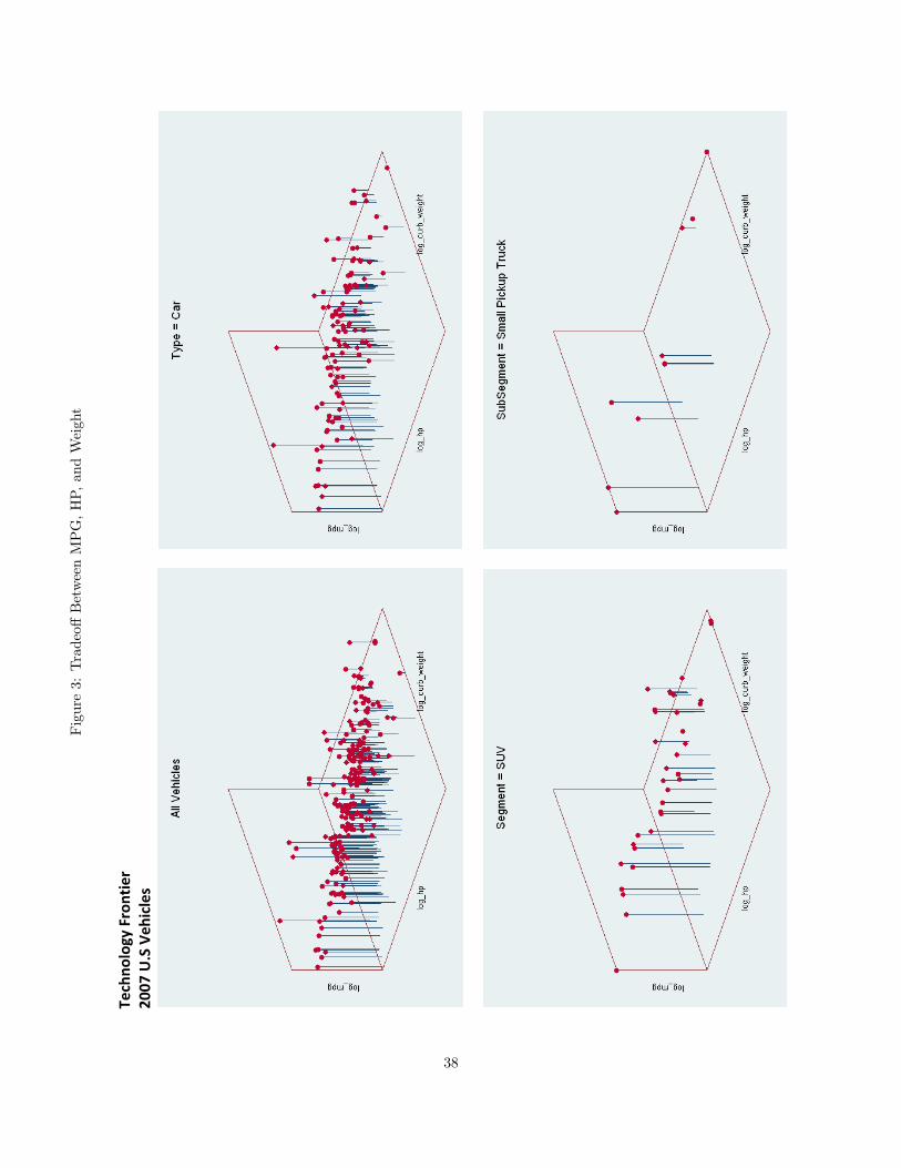
Fig

ure

3:T

rade

offB

etw

een

MP

G,

HP,

and

Wei

ght

Techno

logy Frontier 

2007

 U.S Veh

icles 

      

  

      

 

38

Fig

ure

4:T

imin

gof

the

Gam

e

Timing of Events

Time t‐1

Time t

Ht‐1

ξ t, ω

tmpg

tI t‐

1P g

as,t

p tq t

R t

Inform

ation set

Shocks

Characteristic

Inform

ation set

Shock

Characteristic

Purchases

Ex post regret

in m

pgt cho

ice

Know

nRe

vealed

Chosen

Know

nRe

vealed

Chosen

Chosen

Revealed

by all

by nature

by firm

sby

 all

by nature

by firm

sby

 csrs

by nature

Includ

es:

Includ

es:

Due

 to p

gas,t

*i

dl'

*i

dl'

* tim

e t m

odels' 

sub‐segm

ents

* tim

e t m

odels' 

sub‐segm

ents

* tim

e t m

odels' 

manufacturers

* tim

e t m

odels' 

manufacturers

* p g

as,t‐1

* p g

as,t‐1

* ξ t, ω

t

* mpg

t

39

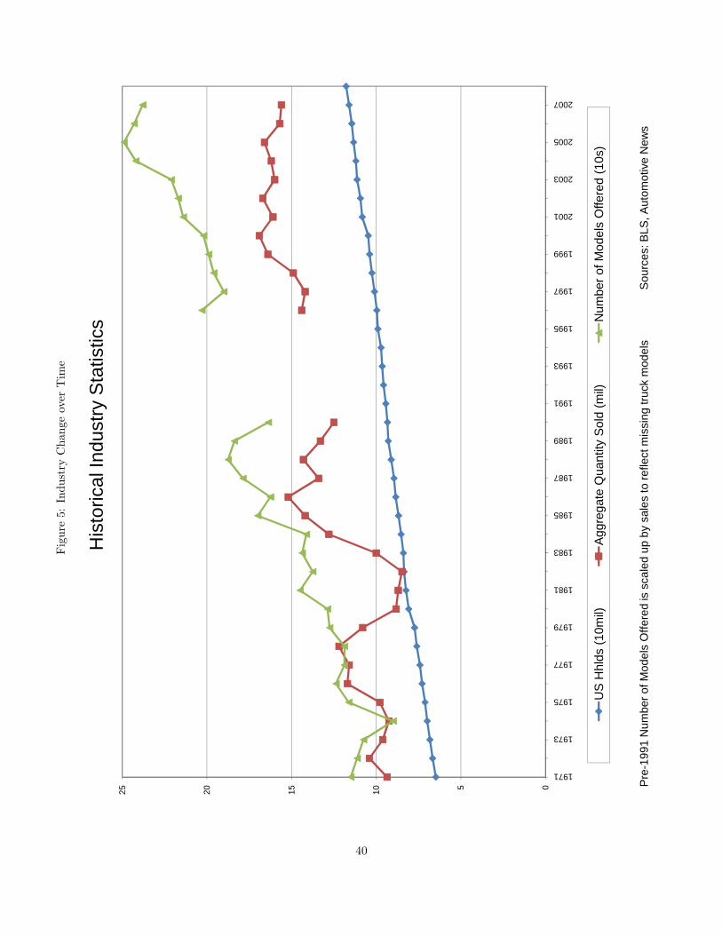
Fig

ure

5:In

dust

ryC

hang

eov

erT

ime

152025

His

toric

al In

dust

ry S

tatis

tics

0510

1971

1973

1975

1977

1979

1981

1983

1985

1987

1989

1991

1993

1995

1997

1999

2001

2003

2005

2007

US

Hhl

ds (1

0mil)

Agg

rega

te Q

uant

ity S

old

(mil)

Num

ber o

f Mod

els

Offe

red

(10s

)

Pre

-199

1N

umbe

r of M

odel

s O

ffere

d is

sca

led

up b

y sa

les

to re

flect

mis

sing

truc

k m

odel

s

Sou

rces

: BLS

, Aut

omot

ive

New

s

40

Fig

ure

6:H

isto

ryof

Fuel

Effi

cien

cyan

dR

egul

atio

n

40

His

toric

al G

as P

rice

& F

uel E

ffici

ency

35 2530 imes 20 nd 2007 d 15 mpg an

510 0

971

973

975

977

979

981

983

985

987

989

991

993

995

997

999

001

003

005

007

19

19

19

19

19

19

19

19

19

19

19

19

19

19

19

20

20

20

20

real

gas

pric

e (2

007

dim

es)

PC

std

LT s

tdP

C a

ctLT

act

PC

= P

asse

nger

Car

s, L

T =L

ight

Tru

cks

S

ourc

es: W

ards

,Aut

omot

ive

New

s, E

IA, N

HS

TA

41

Fig

ure

7:Y

earl

yC

hara

cter

isti

csC

hang

es

20253035

Year

ly C

hara

cter

istic

Cha

nges

Toyo

ta C

elic

a

mpg

Wei

ght (

thou

s lb

s.)

051015

71

72

73

74

75

76

77

78

79

80

81

82

83

84

85

86

87

88

89

90

91

92

93

94

95

96

97

98

99

00

01

02

03

04

05

Pgas

(200

7 di

mes

)

Hp/

10

42

Fig

ure

8:C

hang

ing

Gas

Pri

ce,

Cha

ngin

gO

ptim

a

-0.4

-0.20

0.2

0.4

0.6

0.8

18

19

20

21

22

23

24

25

26

27

∂πf / ∂mpgj

mp

gj

Incen

tive t

o C

han

ge F

uel

Eff

icie

nc

yTo

yo

ta A

valo

n

20

07

20

08

Actu

al2007

22m

pg

Optim

al 2008

23.5

mpg

Optim

al 2007

21.3

mpg

43

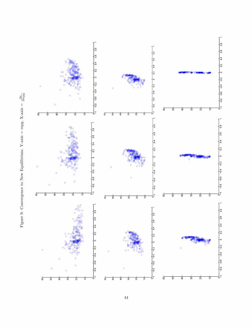
Fig

ure

9:C

onve

rgen

ceto

New

Equ

ilibr

ium

:Y

-axi

s=mpg,

X-a

xis

=∂π

∂mpg

44

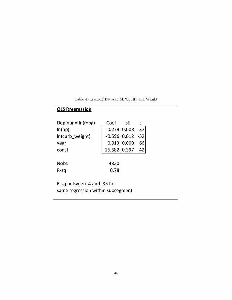
Table 4: Tradeoff Between MPG, HP, and Weight

OLS Rregression

Dep Var = ln(mpg) Coef SE tln(hp) ‐0.279 0.008 ‐37ln(curb_weight) ‐0.596 0.012 ‐52year 0.013 0.000 66const ‐16.682 0.397 ‐42

Nobs 4820R‐sq 0.78

R‐sq between .4 and .85 forsame regression within subsegment

45

Tab

le5:

Pop

ular

Car

sby

Aut

omot

ive

Sub-

Segm

ent

Aut

omot

ive

Type

s, S

egm

ents

and

Sub

-Seg

men

tsSe

gmen

tS

ub-S

egm

ent

Smal

l10

.9%

13.5

%Lo

wer

Sm

all

3.6%

1.1%

GM

C M

etro

Hyu

ndai

Acc

ent

Kia

Sep

hia

Upp

er S

mal

l7.

3%12

.3%

Hon

da C

ivic

GM

C C

aval

ier

Ford

Esc

ort

Toyo

ta C

orol

la

Mid

dle

11.5

%20

.5%

Low

er M

iddl

e4.

7%5.

8%H

onda

Civ

icG

MC

Gra

nd A

mG

MC

Mal

ibu

Hyu

ndai

Son

ata

Nis

san

Alti

ma

Upp

er M

iddl

e6.

8%14

.7%

Toyo

ta C

amry

Hon

da A

ccor

dFo

rd T

auru

sG

MC

Impa

laN

issa

n A

ltim

a

Larg

e3.

1%3.

8%La

rge

Reg

ular

3.1%

3.8%

GM

C L

esab

reC

hrys

ler I

ntre

pid

Chy

sler

300

Ser

ies

Ford

Gra

nd M

arqu

isFo

rd C

row

n V

icto

ria

Luxu

ry23

.6%

7.6%

Low

er L

uxur

y7.

6%3.

5%B

MW

3To

yota

Ava

lon

Vol

vo 7

0A

cura

TL

Lexu

s E

S33

0M

iddl

e Lu

xury

6.4%

2.6%

GM

C F

leet

woo

d D

evill

eFo

rd T

own

Car

GM

C P

ark

Ave

nue

BM

W 5

Mer

cede

s C

Upp

er L

uxur

y3.

8%0.

8%M

erce

des

EG

MC

Sev

ille

BM

W 5

Lexu

s LS

430

Jagu

ar S

Luxu

ry S

port

5.7%

0.7%

Cor

vette

BM

W Z

3C

hrys

ler C

ross

fire

Por

sche

911

Spec

ialty

10.8

%4.

1%S

mal

l Spe

cial

ty3.

3%0.

8%B

eetle

IITo

yota

Sci

onTo

yota

Cel

ica

BM

W M

ini C

oope

rM

azda

MX

3M

iddl

e S

peci

alty

4.5%

2.7%

Ford

Mus

tang

Mits

ubis

hi E

clip

seG

MC

Cam

aro

GM

C M

onte

Car

loTo

yota

Cel

ica

Larg

e S

peci

alty

0.3%

0.1%

Ford

Thu

nder

bird

Ford

Cou

gar

thes

e ar

e th

e on

ly tw

o ca

rs in

this

cla

ss &

they

onl

y ex

ist 9

6-98

Luxu

ry S

peci

alty

2.6%

0.5%

Chr

ysle

r Seb

ring

CN

VT

Acu

ra C

LM

erce

des

CLK

GM

C E

ldor

ado

BM

W 6

CU

V10

.6%

6.5%

Sm

all C

UV

1.4%

1.2%

Chr

ysle

r PT

Cru

iser

GM

C H

HR

Toyo

ta R

AV

4H

onda

Ele

men

tM

iddl

e C

UV

4.3%

3.5%

Ford

Esc

ape

Hon

da C

RV

GM

C E

quin

oxTo

yota

Hig

hlan

der

Larg

e C

UV

1.0%

0.6%

Hon

da P

ilot

Chr

ysle

r Pac

ifica

Ford

Fre

esty

leM

iddl

e Lu

xury

CU

V3.

0%1.

0%Le

xus

RX

330

BM

W X

5V

olvo

XC

90M

erce

des

MLa

rge

Luxu

ry C

UV

0.9%

0.3%

Acu

ra M

DX

GM

C S

RX

Mer

cede

s R

Cla

ss

SUV

13.0

%16

.0%

Sm

all S

UV

1.4%

0.9%

Chr

ysle

r Wra

ngle

rK

ia S

porta

geG

MC

Tra

cker

Suz

uki V

itara

Mid

dle

SU

V4.

9%9.

3%Fo

rd E

xplo

rer

Jeep

Gra

nd C

hero

kee

GM

C T

railb

laze

rC

hrys

ler L

iber

tyLa

rge

SU

V2.

3%4.

5%Fo

rd E

xped

ition

GM

C T

ahoe

Chr

ysle

r Dur

ango

Mid

dle

Luxu

ry S

UV

2.6%

0.7%

Mer

cede

s M

Lexu

s G

X47

0G

MC

Bra

vada

Infin

iti Q

X4

Larg

e Lu

xury

SU

V1.

9%0.

6%Fo

rd N

avig

ator

GM

C E

scal

ade

GM

C H

umm

er 2

Van

9.7%

9.4%

Sm

all V

an6.

1%6.

6%C

hrys

ler C

arav

anFo

rd W

inds

tar P

ass.

Chr

ysle

r Tow

n &

Cou

ntry

Toyo

ta S

ienn

aLa

rge

Van

2.4%

2.2%

Ford

Eco

nolin

eG

MC

Exp

ress

Car

goLu

xury

Van

1.2%

0.6%

Chr

ysle

r Tow

n &

Cou

ntry

GM

C S

ilhou

ette

Maz

da M

PV

Pas

s. V

anTo

yota

Pre

via

Pick

up5.

4%18

.5%

Sm

all P

icku

p3.

3%5.

3%Fo

rd R

ange

rG

MC

S10

Pic

kup

Toyo

ta T

acom

aLa

rge

Pic

kup

2.1%

13.2

%Fo

rd F

Ser

ies

GM

C S

ilver

ado

GM

C C

hevy

CK

Pic

kup

Chr

ysle

r Ram

Pic

kup

Oth

er1.

4%0.

1%C

omm

. Cha

ssis

1.4%

0.1%

Che

vy P

Mod

elIs

uzu

NP

R

Cars Trucks/VansUtility Vehicles

% o

fM

odel

-Yrs

% o

fSa

les

Popu

lar M

odel

s

46

Table 6: Summary Statistics

Summary Statistics

Variable Mean Std. Dev. Min Max

Year 1992.5 11.1 1971 2007

Mpg 20.7 5.8 9.13 61

Dpm $0.10 $0.04 $0.03 $0.24

Price $30,059 $21,195 $7,038 $115,000

q 75,566 95,043 123 890,790

Price gas $2.02 $0.48 $1.31 $3.15

Price gas change $0.05 $0.24 -$0.56 $0.68

GDP Growth 3.1% 1.7% -1.9% 7.2%

N Models in Year 150.6 55.9 72 249

N Model-Years 4,820

N Years 32

N Types 3

N Segments 9

N Sub-segments 28

Note: Prices are Real 2007 Dollars

47

Table 7: Estimation Results

GMM Estimation Results

Demand parameters: Cost parameters:

Variable Coeff S.E. T-stat Variable Coeff S.E. T-stat

price ($10k) α -0.33 0.02 -18.41 ln mpg γ -0.03 0.11 -0.32

ln mpg βm -0.75 0.17 -4.51 year γ 0.03 0.00 14.72

dpm Car small βd -4.70 0.66 -7.13 autonews γ 0.32 0.05 6.14

dpm Car middle βd -5.55 0.55 -10.01 asian γ 0.16 0.02 6.78

dpm Car large βd -4.68 0.65 -7.16 euro γ 0.60 0.03 21.96

dpm Car luxury βd -2.13 0.43 -4.98 Subsegment_dums ‡ γ 9.86 0.21 47.87

dpm Car specialty βd -4.02 0.44 -9.17 (range 9.02 to 10.74)

dpm CUV βd -9.07 2.95 -3.08 CAFÉ λ 347$ 3.40$ 102

dpm SUV βd -8.10 1.13 -7.20

dpm Truck βd -4.17 0.70 -5.98

dpm Van βd -3.65 0.70 -5.20

gdp gr β 2.06 0.36 5.79

gdp per cap β 0.02 0.01 1.45

cuv x year β 0.08 0.03 2.50

suv x year β 0.11 0.01 8.11

autonews datasource β 0.34 0.04 8.33

asian β -0.06 0.01 -4.52

euro β 0.14 0.03 5.30

partial year of sales β -0.57 0.02 -27.06

ln(sj|ss) † σss 0.78 0.00 388

ln(sss|s) † σs 0.92 0.00 1081

ln(ss|t) † σv 0.83 0.00 360

Subsegment_dums ‡ β 1.28 0.23 4.76

(range -4.07 to 0.56)

Notes:

† In addition to being statistically different from 0, log shares are also statistically different from 1.

They are, respectively, 108, 97, and 76 standard errors from 1.

‡ There are 31 Subsegment Dummies. Rather than report them all,

I report means of absolute values of Coeff, S.E., and T-stat.

N observations = 5,244

R2 from 2sls on demand (for starting values) is 0.95

48

Tab

le8:

Will

ingn

ess

toP

ay

Segm

ent

Smal

lM

idd

leLa

rge

Luxu

rySp

eci

alty

CU

VSU

VTr

uck

Van

Mea

n M

PG

*3

1.2

28

.32

0.2

20

.32

2.0

22

.81

6.2

17

.21

8.1

20

% o

f M

ean

MP

G6

.25

.74

.04

.14

.44

.63

.23

.43

.6

p_

gas

$4

.55

1,5

54

$

3,4

57

$

4,0

30

$

55

6$

2,3

80

$

7,5

71

$

9,9

64

$

4,4

40

$

3,4

13

$

$3

.43

72

0$

2,1

54

$

2,5

86

$

(33

)$

1,3

42

$

5,2

56

$

7,0

59

$

2,8

95

$

2,1

21

$

$1

.50

(71

8)

$

(91

)$

98

$

(1

,04

7)

$

(4

46

)$

1

,26

5$

2

,05

4$

2

33

$

(1

05

)$

* 2

00

7 S

ales

-Wei

ghte

d, S

egm

ent-

Ave

rage

MP

G

Neg

ativ

e en

trie

s ar

e d

ue

to

th

e q

ual

ity

red

uct

ion

s re

qu

ired

to

imp

rove

MP

G (

wit

hin

a s

ub

-seg

men

t).

Will

ingn

ess

to

Pay

fo

r 2

0%

MP

G in

cre

ase

By

Segm

ent

and

By

Gas

Pri

ce

49

Tab

le9:

Will

ingn

ess

toP

ayw

itho

utQ

ualit

yIn

crea

se

Segm

ent

Smal

lM

idd

leLa

rge

Luxu

rySp

eci

alty

CU

VSU

VTr

uck

Van

Mea

n M

PG

*3

1.2

28

.32

0.2

20

.32

2.0

22

.81

6.2

17

.21

8.1

20

% o

f M

ean

MP

G6

.25

.74

.04

.14

.44

.63

.23

.43

.6

p_

gas

$4

.55

3,3

90

$

5,2

93

$

5,8

66

$

2,3

92

$

4,2

15

$

9,4

07

$

11

,79

9$

6,2

76

$

5,2

49

$

$3

.43

2,5

56

$

3,9

90

$

4,4

22

$

1,8

03

$

3,1

78

$

7,0

91

$

8,8

95

$

4,7

31

$

3,9

57

$

$1

.50

1,1

18

$

1,7

45

$

1,9

34

$

78

9$

1,3

90

$

3,1

01

$

3,8

90

$

2,0

69

$

1,7

30

$

* 2

00

7 S

ales

-Wei

ghte

d, S

egm

ent-

Ave

rage

MP

G

The

se W

TP's

:

1)

ho

ld q

ual

ity

con

stan

t (w

hile

imp

rovi

ng

MP

G)

2)

ther

efo

re d

o n

ot

refl

ect

the

eco

no

mic

mo

del

3)

are

incl

ud

ed f

or

com

par

iso

n t

o t

he

pre

vio

us

tab

le (

wh

ich

do

ref

lect

th

e ec

on

om

ic m

od

el)

4)

are

stri

ctly

larg

er t

han

th

eir

cou

nte

rpar

ts in

th

e p

revi

ou

s ta

ble

5)

are

stri

ctly

larg

er t

han

0

Wit

ho

ut

Qu

alit

y D

ecr

eas

e:

Will

ingn

ess

to

Pay

fo

r 2

0%

MP

G in

cre

ase

By

Segm

ent

and

By

Gas

Pri

ce

50

Table 10: Model Predictions for $3.43 gas

Model Predictions for $3.43 gas

Type Segment # Models 2007 2008 2009 2007 2008 ‡ 2009 2007 2008 2009

Car 140 7,567 6,861 7,266 22.6 22.6 19.0 26.8 27.6 19.3

-9% -4% 0% -16% 3% -28%

Small 29 2,312 2,357 2,350 28.3 28.3 21.1 31.2 31.8 21.0

Middle 27 2,893 2,136 1,714 24.4 24.4 29.8 28.3 30.4 30.1

Large 14 674 479 320 19.9 19.9 24.1 20.2 20.3 23.8

Luxury 49 1,192 1,440 2,551 19.6 19.6 10.3 20.3 20.4 10.0

Specialty 21 496 451 332 21.4 21.4 18.9 22.0 22.5 18.5

UV 93 4,644 3,577 4,716 18.5 18.5 41.4 19.9 21.9 41.0

-23% 2% 0% 124% 10% 106%

CUV 54 2,636 2,320 2,058 20.6 20.6 43.2 22.8 24.7 43.4

SUV 39 2,008 1,257 2,658 15.5 15.5 39.0 16.2 16.7 39.2

Truck/Van 37 3,673 3,181 3,129 18.0 18.0 20.6 17.4 17.8 21.0

-13% -15% 0% 14% 2% 20%

Pickup 21 2,730 2,264 2,290 18.4 18.4 21.7 17.2 17.6 21.6

Van 16 943 916 839 17.6 17.6 19.1 18.1 18.4 19.2

All Vehicles 270 15,883 13,619 15,110 20.6 20.6 26.9 22.6 23.8 26.4

-14% -5% 0% 31% 5% 17%

† All percentages (shaded) are percentage changes from 2007 levels

‡ 2008 Fuel Efficiency Offerings are fixed at 2007 levels for comparability

Quantity = Sales (1000s)

MPG Offered = Raw-average MPG across models

MPG Purchased = Sales-weighted MPG

2007 - actual

2008 - predicted (before firms adjust characteristics - only consumers respond)

2009 - predicted (after firms adjustt characteristics)

For comparison, actual 2008 (Aug-YTD) Quantities were:

-3%, -19%, -16%, and -14%, for, respectively,

Cars, Utility Vehicles, Trucks/Vans, and All Vehicles.

MPG MPG

Vehicle Classification Quantity †

Offered †

Purchased †

51

Table 11: Model Predictions for $4.55 gas

Model Predictions for $4.55 gas

Type Segment # Models 2007 2008 2009 2007 2008 ‡ 2009 2007 2008 2009

Car 140 7,567 5,878 6,020 22.6 22.6 25.0 26.8 28.6 25.6

-22% -20% 0% 11% 7% -5%

Small 29 2,312 2,229 1,947 28.3 28.3 27.8 31.2 33.2 27.8

Middle 27 2,893 1,252 1,420 24.4 24.4 39.6 28.3 35.0 39.9

Large 14 674 233 265 19.9 19.9 31.6 20.2 20.4 31.6

Luxury 49 1,192 1,811 2,114 19.6 19.6 13.4 20.3 20.6 13.2

Specialty 21 496 353 275 21.4 21.4 25.0 22.0 23.6 24.6

UV 93 4,644 2,348 3,907 18.5 18.5 55.1 19.9 25.8 54.4

-49% -16% 0% 198% 30% 173%

CUV 54 2,636 1,873 1,705 20.6 20.6 57.4 22.8 28.0 57.5

SUV 39 2,008 475 2,202 15.5 15.5 51.8 16.2 17.3 51.9

Truck/Van 37 3,673 2,475 2,593 18.0 18.0 27.3 17.4 18.6 27.8

-33% -29% 0% 51% 7% 59%

Pickup 21 2,730 1,622 1,897 18.4 18.4 28.7 17.2 18.5 28.7

Van 16 943 853 695 17.6 17.6 25.3 18.1 18.7 25.4

All Vehicles 270 15,883 10,701 12,520 20.6 20.6 35.7 22.6 25.7 35.0

-33% -21% 0% 73% 14% 55%

† All percentages (shaded) are percentage changes from 2007 levels

‡ 2008 Fuel Efficiency Offerings are fixed at 2007 levels for comparability

Quantity = Sales (1000s)

MPG Offered = Raw-average MPG across models

MPG Purchased = Sales-weighted MPG

2007 - actual

2008 - predicted (before firms adjust characteristics - only consumers respond)

2009 - predicted (after firms adjustt characteristics)

MPG MPG

Vehicle Classification Quantity †

Offered †

Purchased †

52