November 2017

OIES PAPER: WPM 74

Gasoline Demand in Non-OECD Asia: Drivers and Constraints

Anupama Sen, OIES

Michal Meidan, OIES Research Associate and Energy Aspects &

Miswin Mahesh, Energy Aspects

Gasoline Demand in Non-OECD Asia

i

The contents of this paper are the authors’ sole responsibility. They do not necessarily represent the

views of the Oxford Institute for Energy Studies or any of its members.

Copyright © 2017

Oxford Institute for Energy Studies

(Registered Charity, No. 286084)

This publication may be reproduced in part for educational or non-profit purposes without special

permission from the copyright holder, provided acknowledgment of the source is made. No use of this

publication may be made for resale or for any other commercial purpose whatsoever without prior

permission in writing from the Oxford Institute for Energy Studies.

ISBN 978-1-78467-096-2

DOI: https://doi.org/10.26889/9781784670962

Gasoline Demand in Non-OECD Asia

ii

Contents

Abstract .................................................................................................................................................. 1

1. Introduction ....................................................................................................................................... 2

2. Drivers of Gasoline Demand ............................................................................................................ 3

2.1 Transport as a Key Driver ............................................................................................................. 3

2.2 Other Determinants of Gasoline Demand ..................................................................................... 9

3. Empirical Estimation ....................................................................................................................... 10

4. Constraints to Gasoline Demand Growth in Transport: The Cases of India and China .......... 14

4.1 India – the Race to Leapfrog to Electric Vehicles ....................................................................... 14

Current EV Market ......................................................................................................................... 14

Implications for the power sector ................................................................................................... 16

Policy measures to enable EV penetration .................................................................................... 17

4.2 China – Implications of New Energy Vehicles and Fuel Efficiency ............................................. 17

New Energy Vehicle (NEV) Plan and Impact on Gasoline Demand ............................................. 18

Impact of higher fuel efficiencies, NGVs and bike-sharing ............................................................ 21

5. Conclusion: between slower gasoline growth and new paradigms .......................................... 22

References ........................................................................................................................................... 24

Appendices .......................................................................................................................................... 28

A. Data Sources ................................................................................................................................ 28

B. Descriptive Statistics ..................................................................................................................... 28

C. List of Countries ............................................................................................................................ 28

D. Correlation Matrix ......................................................................................................................... 29

E. Postestimation Tests .................................................................................................................... 29

F. Econometric Method ..................................................................................................................... 30

G: Fractional Polynomial Prediction Plots on Gasoline Consumption per Capita ............................ 31

Figures and Tables

Figure 1: Car ownership/population ratios, 2002 vs. 2015 ..................................................................... 4

Figure 2: Income elasticity of car ownership vs per capita income, 2002-15 ......................................... 5

Figure 3: Car Ownership & GDP per capita: Historical Data & Projections to 2021 ............................... 6

Figure 4: Historical Data & Projections to 2021; based on income elasticity from 1.0-2.0* .................... 6

Figure 5: Car Ownership Levels (Historical and Projected) Fitted Values from a Gompertz Function ... 8

Figure 6: Indian gasoline demand, y/y, mb/d ........................................................................................ 15

Figure 7: Indian car sales, ex-two wheelers, thousand ......................................................................... 15

Figure 8: China NEV sales, thousand units .......................................................................................... 18

Figure 9: China car sales, million units ................................................................................................. 19

Figure10: China gasoline demand, y/y change, mb/d .......................................................................... 22

Figure 11: Asian gasoline demand, mb/d ............................................................................................. 22

Table 1: Car Ownership projections for Asia (and Pacific) based on historical income elasticity .......... 7

Table 2: Description of Untransformed Variables ................................................................................. 11

Table 3: Results from Estimations ........................................................................................................ 13

1

Abstract1

Global oil demand is undergoing a structural shift. This is broadly reflected in changing demand

dynamics over the last 15 years. While OECD demand decreased by 3 million barrels per day (mb/d)

from 2000-15, demand in non-OECD countries grew by 21 mb/d (IEA, 2015). This shift is

characterised by two developments: first, the rapid growth in China’s oil consumption from 2000-13,

and second, the subsequent ‘jump’ in India’s oil demand growth – which overtook China’s in 2015 to

emerge as the main engine of non-OECD Asian oil demand growth. As the emerging market

economies of non-OECD Asia continue to industrialise, rising per capita incomes are likely to further

underpin this structural shift. The shift is particularly visible in gasoline demand – driven primarily by

transport – which has defied expectations in terms of the sources of demand growth. Contrary to

those expectations, the centre of growth has shifted from West of Suez markets to non-OECD Asia,

which had previously been dominated by distillates. Average gasoline demand growth in Asia has

nearly doubled from 130 kb/d a year from 2005-10, to 290 kb/d from 2011 onwards. At the same time,

climate change mitigation and growing concerns over air quality imply that Asia’s economic growth

will occur in a carbon-constrained world, and non-OECD Asia may not follow the trajectories of the

OECD countries. Given this context, this paper investigates two research questions: first, what are the

key drivers of gasoline demand growth in non-OECD Asia, based on historical trends? And second,

what are the constraints to gasoline demand growth in this region? The first question is investigated

using statistical analyses on a panel dataset of 19 countries in the Asia-Pacific region, of which over

half are non-OECD countries. The second question, driven by regional policies, is investigated by

looking in depth at the cases of India and China. The paper gives a broad insight into the drivers and

constraints on Asian gasoline demand, focusing on the transport sector as a key variable.

1 The authors are grateful to Bassam Fattouh for comments on an earlier draft of this paper, and to Kate Teasdale and Justin

Jacobs for their help with publication.

2

1. Introduction

Global oil demand is undergoing a structural shift. Over the last 15 years, while OECD demand

decreased by 3 million barrels per day (mb/d) from 2000-15, demand in non-OECD countries grew by

21 mb/d (IEA, 2015). This shift is characterised by the rapid growth in China’s oil consumption from

2000-13, and the ‘jump’ in India’s oil demand growth – which overtook China in 2015 to emerge as

the main engine of non-OECD Asian oil demand growth. As the emerging market economies of non-

OECD Asia continue to industrialise, rising per capita incomes will further underpin this structural shift.

The shift is particularly visible in gasoline. Growth in gasoline demand has defied expectations –

which were for demand to decline as it was mainly driven by West of Suez markets while East of

Suez demand was distillate-heavy. Gasoline growth is now being driven by non-OECD economies in

Asia. Asian gasoline demand, which was growing at an average of 130 kb/d a year between 2005 and

2010, nearly doubled to 290 kb/d a year from 2011 onwards.

In consumer theory, the demand for gasoline is a ‘derived’ demand (Storchmann, 2005; Becker, 1965;

Lancaster, 1966; Muth, 1966). It is not gasoline itself which gives benefit to the consumer, but the

end-product – namely, mobility (Storchmann, 2005). Hence the key drivers of gasoline demand

growth pertain to specific products or sectors. For instance, in India three key sectors have been

identified as driving growth in the derived demand for oil (Sen and Sen, 2016):

Transportation (rising car ownership levels and the growth of the vehicle fleet);

Infrastructure (road construction); and,

Manufacturing (the push to expand manufacturing’s share within Gross Domestic Product (GDP)).

While the literature2 suggests an increase in the growth or stock of oil-consuming sectors or products

based on historical trends, there are increasing policy constraints on the pace of such trends as the

world economy enters a carbon-constrained era of economic growth. Thus, the same trends which

applied to the advanced OECD countries may not necessarily hold for non-OECD Asia.

On the one hand, non-OECD Asian economies are expected to enter or continue along high-growth

trajectories over the next decade, driven by significant expansions in infrastructure, output and

income at the national level; examples include India’s nationwide programme to add 30 km of

roads/day, and its push to increase manufacturing’s share of GDP from 15% to 25% by early next

decade through focusing on energy-intensive industry, as well as China’s ‘One Belt One Road’

initiative to create connecting infrastructure across Asia. On the other hand, given the carbon

constraint on economic growth arising from the ratification of the Paris Agreement, there is a push

towards increasing the efficiency of energy use (such as through stricter fuel efficiency standards in

transportation and eliminating fossil fuel subsidies from end-user prices), as well as a greater number

of local or regional level initiatives to curb environmental externalities (such as the adoption of Electric

Vehicles (EVs), and bans on polluting vehicles). Notably, while the push to increase output and

income is primarily occurring at the national level in most non-OECD Asian countries, the constraints

to this expansion are currently being driven at the local or regional level. These counteracting trends

and the complexity of the policies which underpin them make it unlikely that non-OECD Asian

economies will follow the same historical trends in oil consumption as the OECD. There are three

potential arguments that can be made:

One argument is that these economies will enter high-growth trajectories, but that these trajectories could be shorter, and the plateaus in consumption may come sooner than they have in the OECD.

2 For instance, see Dargay et al (2007), Dargay (2001), and Huo et al (2007).

3

A second argument is that technological advancements (such as in storage technologies) will facilitate a faster substitution of oil in its core consuming sectors (for example, gasoline in the transport sector) regardless of the growth in car ownership.

A third argument is that the fragmented nature of regional-level policy constraints will fail to have a significant impact on nationally-driven movements to industrialise.

Given this context, this paper aims to investigate two research questions: first, what are the key

drivers of gasoline demand growth in non-OECD Asia, based on historical trends? And second, what

are the key constraints to gasoline demand growth in this region? The first question, driven by

historical trends, is investigated by applying statistical analyses to a panel dataset of 19 countries in

the Asia-Pacific region, of which over half are non-OECD countries. The second question, driven by

local and regional policies, is investigated by looking at the cases of India and China, in which we also

examine the plausibility of the three potential arguments. The paper gives a broad insight into the

drivers and constraints on Asian gasoline demand, focusing on the transport sector as a key variable.

2. Drivers of Gasoline Demand

2.1 Transport as a Key Driver

The transport sector accounts for roughly 63% of global oil consumption, and has historically been the

fastest growing oil-consuming sector (WEC, 2016). By 2035, it has been projected that 88% of the

world’s oil demand growth will come from transportation, largely from developing economies (BP,

2016). Medlock and Soligo (2001) show that per capita energy demand in the transport sector steadily

increases throughout the process of economic development, eventually accounting for the largest

share of total final energy consumption. As oil demand for road transportation is closely linked with

the number of cars and other road vehicles in use, projections of future growth in the vehicle stock

can provide an insight into future fuel requirements (Dargay and Gately, 1999). In OECD countries,

the growth of the vehicle stock, measured in terms of vehicle (or more specifically, car) ownership,

has followed a clear path, varying closely with changes in per capita income. As per capita income

increased beyond a ‘trigger’ threshold, car ownership grew exponentially. However, as per capita

income in these countries continued to increase to higher levels and reached a second ‘trigger’

threshold, car ownership levels have begun to level off. This relationship has been formalised in the

existing literature: vehicle ownership grows relatively slowly at the lowest levels of per capita income,

then about twice as fast at middle income levels (for instance, estimated at $3,000 to $10,000 per

capita in Dargay and Gately (2007)), and finally, about as fast as income at higher income levels,

before reaching saturation at the highest levels of income (Dargay and Gately, 1999; Dargay et al,

2007; Medlock and Soligo, 2002; Storchmann, 2005; Button et al, 1993).

The historical relationship between per capita income and vehicle ownership implies that ceteris

paribus, as the developing non-OECD countries climb to higher levels of per capita income, vehicle

ownership could follow a similar trajectory to the OECD, increasing oil demand for transportation.

Historical data supports this argument – for instance, Dargay et al (2007) showed that this relationship

held for 45 countries in which non-OECD countries comprised more than a third, and for three-fourths

of the sample’s population, for the time period 1960-2002. In the 15 years since, some have entered

lower middle-income levels (based on Purchasing Power Parity or PPP). A more recent dataset on

vehicle (car) ownership and per capita income was assembled for this paper, covering the period

2002-20153 for 19 Asian countries (the majority of which are non-OECD). This period is especially

significant because non-OECD oil demand increased by roughly 21 mb/d from 2000-2015, while

3 Our analysis covers a shorter time period as public data on vehicle ownership across non-OECD countries is not easily

available. Other notable studies have covered much shorter time periods (for instance Storchmann (2005) uses data for 7

years), and therefore a shorter time-series should not detract from our results.

4

OECD oil demand decreased by 3 mb/d, with this secular decline expected to continue at around 5

mb/d by 2035 (BP, 2016). The two largest non-OECD economies, China and India, are expected to

account for 50% of the increase in oil demand to 2035 (BP, 2016).

Figure 1: Car ownership/population ratios, 2002 vs. 2015

Source: Authors

Figure 1 above summarises the changes in car ownership from 2002-15 for the countries in the

dataset.4 5 Each country’s 2002 car/population ratio is plotted on the vertical axis and its 2015 ratio on

the horizontal axis. The higher up the country is on the diagonal (1:1 line), the higher its car ownership

levels. The greater its distance from the diagonal, the faster was its increase in car ownership relative

to per capita income. For instance, Australia’s car ownership ratio in 2015 was very high relative to

most other countries, at approximately 0.565 (or 565 cars per 1,000 population); however, its average

annual growth from 2002-15 was only 0.71% (up from 0.517 in 2002). China’s car ownership ratio

was relatively low in 2015 (approximately 0.083); however, the average annual growth from 2002-15

was 60% (from 0.009 in 2002). Similarly, India’s car ownership ratio was only 0.02 in 2015, but

average annual growth from 2002-15 was around 14%. In Vietnam, the corresponding figures were

roughly 0.021 (2015) and nearly 18% annual average growth (2002-15). This is a very broad measure

of the car ownership to per capita income relationship and does not take into account the specific

anomalies and circumstances of each country. For instance, Brunei (a resource-rich country) appears

to have experienced a rapid increase in car ownership levels during the period in question despite

being a relatively high-income country – this could be due to many other factors such as economic

conditions, pricing/subsidies6 or government policy. Or it could simply be due to issues with the

reliability of published data.

Figure 2 provides a more detailed picture of the responsiveness of car ownership to changes in

income levels, as it plots the historical ratio of the average annual percentage growth in car ownership

to the average annual percentage growth in per capita income, which is widely considered a broad

measure/estimate of the income elasticity of car (or vehicle) ownership (Dargay and Gately, 1999).

4 See Table C in appendices. The graph is based on Dargay et al (2007) and Dargay and Gately (1999). 5 The figure includes 18 countries, as sufficient data was unavailable on Papua New Guinea. 6 Resource-rich countries have tended to subsidise fuel prices to citizens, leading to excessive increases in domestic fuel

consumption and a potentially lower price-relative-to-income elasticity of car ownership. Due to high private consumption, the

vehicle fleet tends to be dominated by private cars (IBP, 2015).

Australia

Bangladesh

Brunei

China

Taipei

Hong Kong (China)

IndiaIndonesia

Japan

Korea

Malaysia

Myanmar

New Zealand

Pakistan

Philippines

Singapore

Thailand

Vietnam

0

0.1

0.2

0.3

0.4

0.5

0.6

0.7

0 0.1 0.2 0.3 0.4 0.5 0.6 0.7

Car

ow

ner

ship

/po

pn

rat

io 2

00

2

Car ownership/popn ratio 2015

5

Growth rate ratios are plotted for the majority of countries in our dataset on the vertical axis, and

compared with each country’s average income (measured by per capita GDP on the horizontal axis)

over the period 2002-15. The figure shows that car ownership grew almost twice as fast as income for

the lower and middle-income countries (that is, income elasticity was around 2.0). For China, it grew

3.7 times as fast7, whereas for Vietnam it was nearly 2.5.8 For India, it was around 1.7 times as fast.

The figure also shows that the higher a country’s income level, the lower its income elasticity of car

ownership – at very high levels of income, car ownership begins to approach zero as saturation is

reached.

Figure 2: Income elasticity of car ownership vs per capita income, 2002-15

Source: Authors

These broad estimates (based on historical data from 2002-15) of income elasticity of car ownership

can be combined with forecasts on GDP and population to project forward estimates of car ownership

levels in both OECD and non-OECD Asian countries, holding constant all other factors that may be

likely to influence the growth in the car (or vehicle) fleet (we return to these later). Accordingly, we

used International Monetary Fund (IMF) forecasts for GDP to 2021 and UN Population forecasts to

the same period to obtain simple projections for car ownership to 2021. Figure 3 graphs the historical

data along with these broad projections, with car ownership plotted on the vertical axis and per capita

income on the horizontal axis. The multiple series plotted represent both low and high-income

countries and the trend can be seen as mimicking an ‘S’ curve (illustrated by the polynomial trend

line).

Each solid line in the graph can be interpreted as representing a country time series (historical and

projection) for car ownership levels vis-à-vis per capita GDP, between 20029 and 2021. In order to

simulate the ‘S’ curve, we included data on both low and high-income countries (non-OECD and

OECD) in the Asia-Pacific region (for instance, New Zealand and Australia are the two series at the

top of the graph). It can be seen that countries with relatively higher income elasticity of car ownership

7 These high values are not limited to Asia. Eskeland and Feyzioglu (1997) for instance showed a similarly high-income

elasticity (3.34) for Mexico. 8 The figure shows the Philippines as an outlier in the dataset with very low-income elasticity; based on available data, its car

ownership ratio grew by only 0.23% on average annually from 2002-15. The Nielsen Global Survey of Automotive Demand

(2013) estimates that 47% of households did not own cars. 9 The starting year is 2005 for some countries which lacked historical data.

Australia

Bangladesh

China

Taipei

Hong Kong (China)

IndiaIndonesia

JapanKorea

Malaysia

New Zealand

Pakistan

PhilippinesSingapore

Thailand

Vietnam

0.00

0.50

1.00

1.50

2.00

2.50

3.00

3.50

4.00

0 10 20 30 40 50 60 70 80

Avg

inco

me

elas

tici

ty o

f ve

hic

le o

wn

ersh

ip,

20

02

-15

Avg per capita GDP, 2002-15 (thousands, PPP$2011)

6

are clustered in the bottom left of the graph. Figure 4 below expands further upon these countries to

give a clearer picture; it plots historical data and projections on car ownership levels (2002-2021)

focusing on countries with an estimated income elasticity of car ownership between 1.0 and 2.0.

Figure 3: Car Ownership & GDP per capita: Historical Data & Projections to 2021

Source: Authors

Figure 4: Historical Data & Projections to 2021; based on income elasticity from 1.0-2.0*

Source: Authors; *Inset graph shows China

1

51

101

151

201

251

301

351

401

451

501

551

601

651

701

0 20000 40000 60000 80000 100000 120000

Car

ow

ner

ship

(p

er 1

00

0):

20

02

-21

GDP per capita ($'000)

AusBangladeshChinaC.Taipei/TaiwanHong Kong (China)IndiaIndonesiaJapanKoreaMalaysiaNZPakistanPhilippinesSingaporeThailandVietnam

7

Some broad observations can be made here. Although Vietnam’s car ownership level in 2005 was

lower than India’s, its projected car ownership levels rise much faster with its per capita GDP, as it

has an estimated historical income elasticity of roughly 2.5 compared with India’s at 1.7. Thus,

Vietnam’s projected car ownership level goes from roughly 6 per 1000 (in 2005) to 50 per 1000

people, compared with India’s which rises from 9 to around 44 per 1000 people by 2021. Thailand has

the highest starting car ownership level among the group of countries, rising from roughly 60 to 180

per 1000 by 2021, at an estimated income elasticity of roughly 2.0. It is followed by Indonesia, which

with an estimated income elasticity of 1.7 rises from 23 cars per 1000 people in 2005 to over 100 by

2021. Although Bangladesh similarly has an estimated income elasticity of nearly 2.0, its very low

levels of car ownership (around 1 per 1000) and projected per capita income see car ownership levels

rising to just over 6 per 1000 by 2021, according to this broad calculation. Car ownership levels in

Pakistan rise from around 9 to 19 per 1000 by 2021 based on an estimated income elasticity of 1.4.

The non-OECD Asian country with the highest income elasticity is China, and although it has not

been plotted within Figure 4 to allow for a clearer scale, it is included as an inset (within the figure

above), showing car ownership rising from very low levels (around 10 per 1000) in the early 2000s to

well over 300 per 1000 by 2021, based on an estimated (historical) income elasticity of 3.7. 10 Table 1

below depicts the broad estimates shown in Figure 4 for 2002 and 2021.

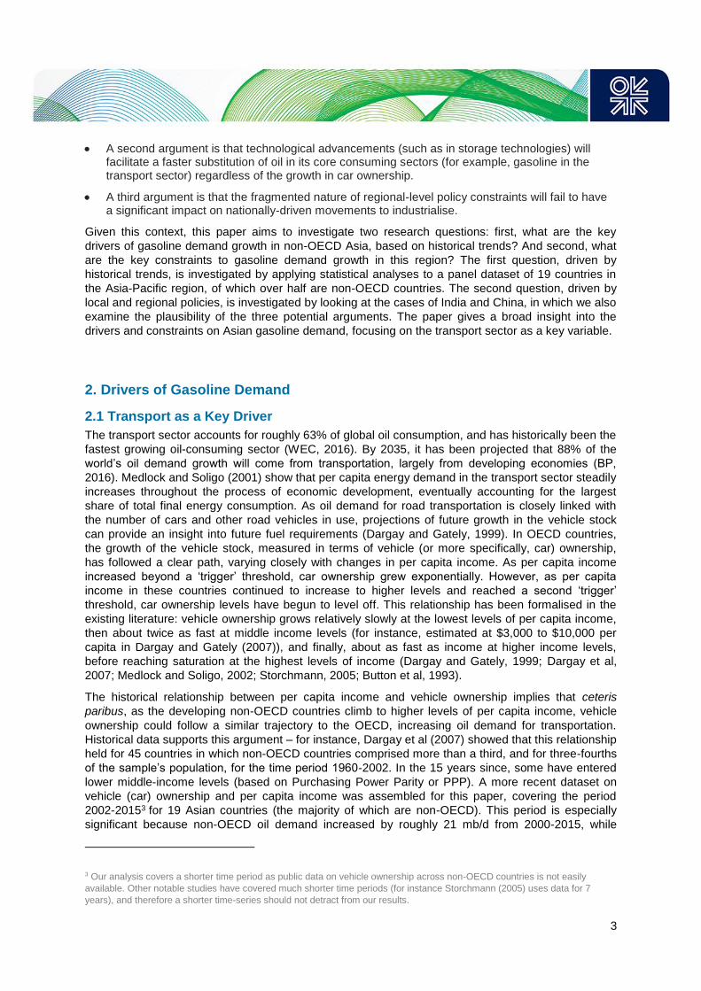
Table 1: Car Ownership projections for Asia (and Pacific) based on historical income elasticity

Estimated

Historical Income

elasticity

GDP per

capita 2002

($)

Cars per

1,000 people

(2002)

GDP per

capita 2021

($)

Cars per

1,000 people

(2021)

Australia 0.46 36,364 518 56,408 618

Bangladesh 2.02 1,730 1 5,587 6

China 3.69 4,285 9 21,733 368

Taipei 0.27 21,066 248 59,166 343

Hong Kong

(China) 0.58 34,366 54 71,202 80

India 1.61 2,651 7 9,837 43

Indonesia 1.73 6,119 23 15,848 100

Japan 0.57 32,248 450 44,574 578

Korea 0.70 23,008 236 47,176 380

Malaysia 0.81 16,417 254 35,058 539

New Zealand 0.55 29,637 583 43,931 740

Pakistan 1.39 3,533 9 6,648 19

Philippines 0.05 4,322 30 10,341 32

Singapore 0.25 51,435 103 104,537 122

Thailand 1.95 9,905 60 21,303 180

Vietnam 2.47 2,920 6 9,065 51

Source: Authors

The estimates in Figure 4 (and Table 1) are broadly indicative of individual country projections on car

ownership and per capita income. They are considerably higher than, for instance, Dargay et al

(2007), who project vehicle ownership to 2030.11 We can however obtain further information on the

10 This is significantly higher than Dargay et al (2007) who base their projections on an income elasticity of 2.2 for China, but

close to Wang et al (2011) who estimate an income elasticity of 3.96 for their projections to 2022. Some of Dargay et al

(2007)’s projections for 2002-2030 have underestimated actual growth (see footnote 11). 11 For instance, Dargay et al (2007) estimate India’s car ownership per 1,000 people at 17 in 2030. However, actual car

ownership levels for in India even as early as 2015 were higher than the 2030 projection (20 per 1,000 people) implying that our

projection is not implausible (albeit based on a simple statistical extrapolation).

8

dataset (historical and projected) as a whole by fitting an arbitrary nonlinear regression function by

least squares. This is based on the ‘S’ curve or Gompertz distribution (an asymmetric sigmoid shape)

which allows for asymmetry in the curve.12 The results are shown in Figure 5 below.

The fitted line (overlaid on a scatter plot of the data) suggests a lower ‘plateau’, or level of saturation,

of car ownership in Asia than seen in other OECD countries – at around 400 cars per 1000 people.

Previous estimates for countries in Western Europe put the plateau in excess of 500 per 1000 people

and close to 800 in the USA. This observation, an estimate rather than a prediction, has interesting

implications: non-OECD Asian countries represent around 60% of global population, two-thirds of the

world’s poor population and yet only 34% of global energy demand. Storchmann (2005) argues that

the income elasticity of demand for vehicles in developing countries is higher than in developed

countries because of the extremely high marginal rate of consumption of automobiles in the former

lower-income countries. As opposed to developed countries, in lower-income countries cars are seen

as a luxury good and their stock is far away from saturation – cars constitute a first purchase or

necessity (i.e. citizens of developing countries purchase their first vehicles as their incomes increase,

often moving up the ladder of mobility from two wheelers to four wheelers). This suggests substantial

potential for growth in car ownership – yet results from the arbitrary nonlinear regression indicate that

this potential could be constrained relative to OECD trajectories, with knock-on effects on oil

consumption in transport. We return to factors that could potentially constrain gasoline consumption in

transport later in the paper (in the case studies).

Figure 5: Car Ownership Levels (Historical and Projected) Fitted Values from a Gompertz Function

Source: Authors

12 We Stata’s nl command with gom3 option. The model estimated is Y = β1*exp (-exp (-β2*(X- β3))).

9

2.2 Other Determinants of Gasoline Demand

Previous empirical studies on oil demand using cross-sectional or time series data have focused on

estimating the relationship between per capita income and vehicle ownership, using the latter as a

key indicator for derived demand. This is based on the assumption that given the historical dominance

of per capita income in determining vehicle ownership, this simplification should not detract from the

validity of the projections obtained (Dargay and Gately, 1999). Within the stock of vehicles, passenger

cars are the largest consumers of oil products and have the highest growth rate (Storchmann, 2005).

Further, passenger cars increase more rapidly than goods vehicles (trucks), as the production of

services grows faster with income than the production of goods (Ingram and Liu, 1997).13 The fact

that cars are traded goods allows for the use of market exchange rates, also making comparisons of

cross-country data easier. The economic rationale behind the use of ‘S’ curves for estimating vehicle

ownership is provided by product life-cycle and diffusion theories, where the take-up rate for new

products is initially slow, then increases as the product becomes more established, and finally

diminishes as the market comes closer to saturation (de Jong et al, 2004).14

Despite the predominant share of passenger vehicles in gasoline consumption, there are arguably

other determinants of gasoline demand that should be taken into account. Several of these are

consistently identified in the existing literature, which utilises pooled cross-sectional or panel datasets

to measure the effects of economic and demographic variables on the levels and rates of vehicle

ownership and/or gasoline demand. Button et al (1993) while focusing on vehicle ownership as the

main dependent variable consider per capita income, fuel price, urbanisation, and the degree of

industrialisation of a country as the main explanatory variables. Similarly, Ingram and Liu (1997)

consider per capita income, motor vehicle prices, population density, the provision of roads, and the

provision of ‘motor vehicle transport services’15 as key explanatory variables determining motorisation.

Dargay and Gately (1999) list several variables that could potentially be considered as influencing

vehicle ownership and thus the derived demand for gasoline: costs (fixed and variable); demography

(the adult/population ratio); population density; urbanisation; and, road density. Storchmann (2005)

takes a slightly different approach: in addition to per capita income, fuel prices, the fixed cost of new

cars and population density as explanatory variables determining gasoline demand, it considers

income inequality (or the distribution of income) as important explanatory variables.16 Medlock and

Soligo (2002) base their estimates on the assumption that individuals purchase vehicles subject to

their budget constraint and some function that describes the rate at which the vehicle is devalued;

individuals therefore invest in the vehicle stock in each period in order to facilitate a flow of services.

Thus, the demand for vehicle stocks is a function of the consumer’s wealth and the user cost of motor

vehicles (for which fuel prices are used as an indicator). 17 Ingram and Liu (1999) probe the

determinants of motorisation and road provision by regressing per capita income, population density,

and fuel prices on the ratio of vehicles to roads. Wang et al (2011) on the other hand question the

premise that vehicle ownership will level off at higher levels of per capita income and use data for

China to project forward rates of vehicle ownership that are far higher than other studies.18 Similarly,

13 Moavenzadeh and Gletner (1984) for instance point out that in general, passenger traffic grows at two to three times that of

freight traffic in developing countries (Button et al, 1993). 14 Interestingly, Ingram and Liu (1999) observed that the estimated ‘saturation’ levels tend to increase over time. 15 Measured by a combination of vehicles and roads (vehicle/road ratio). 16 De Jong et al (2004) argue that for developing countries, the income of the top 20% of the population may be a better

explanatory variable than overall income. 17 Medlock and Soligo (2002) draw from ‘lifetime utility theory’: individuals maximise the present value of their lifetime utility

which is derived from flows of consumption goods and services provided by a stock of physical assets – in this case, motor

vehicles. 18 Primarily based on higher GDP growth forecasts than most other studies, as well as fewer constraints regarding ‘vehicle

saturation’ levels (i.e. they assume that China will be able to absorb huge numbers of vehicles, barring aggressive policy

intervention to restrain car ownership).

10

Huo and Wang (2012) look at total car stock as a function of income distribution, fuel prices and

population in China.

Existing empirical studies provide useful insights not just on the determinants of the demand for

gasoline, but also on the relationships between variables, which are distinctively different for

developed versus developing countries.

The relationship between car ownership and fuel prices is different for developed versus developing countries. Demand for cars tends to be price elastic in the former, whereas developing countries have a higher income elasticity of demand relative to price elasticity.

Urbanisation has different relationships with car ownership when observed across country income groups. In developed countries, car ownership tends to drop with higher rates of urbanisation, particularly as public transportation improves. In developing countries, urbanisation tends to occur alongside growth in car ownership.

Income distribution also tends to demonstrate different relationships with gasoline demand. Storchmann (2005) specifically argues that in developing countries an unequal income distribution is needed to enable people to buy automobiles and thus drive car ownership growth, whereas in developed countries an unequal income distribution would exclude some people from acquiring automobiles. Thus, depending on a country’s income level, inequality has a diverging impact on the ability to buy durable goods, which affects gasoline demand.

Empirical work of the type in the literature cited above is primarily based on the determinants of past

growth, based on the reasonable assumption that this can help researchers understand how policy

interventions may influence future growth. However, it is important to note that these empirical models

do not capture another important aspect of the determinants of the derived demand for gasoline –

namely, consumer behaviour or attitudinal variables. The data requirements for behavioural studies

are onerous, as they rely on consistent attitudinal surveys carried out within countries, and are

therefore beyond the scope of this paper.19 Nevertheless, it can be argued that price and income

elasticities of demand estimated in a partial equilibrium approach capture some behavioural elements

related to consumer spending decisions.

3. Empirical Estimation

This section explores the impact of other determinants on the derived demand for gasoline using a

simple empirical estimation. Previous empirical work (discussed above) identified a consistent set of

variables used as determinants of the derived demand for gasoline (see Table 2). We collated data

on these variables for 19 countries in the Asia-Pacific region, of which more than half are non-OECD

countries (see Appendix C for details), covering the years 2002-15. The data therefore represent a

panel containing both cross-sectional and time series information, where each cross section

represents a country.20

19 De Jong et al (2004) provide a comprehensive survey of models that can be applied to account for the behavioural aspect of

gasoline demand. 20 Panel data analyses present certain advantages. Studies that have used only time series data tend to solely emphasize

short-run elasticities whereas those which use only cross-section data place emphasis on long-run elasticities. A panel dataset

provides a broader picture, allowing for a more general interpretation of results. Panel data techniques are also better placed to

deal with unobserved heterogeneity in the micro-units (Kennedy, 2008).

11

Table 2: Description of Untransformed Variables

Variable Name Variable Label Units

Dependent Variable

Gasoline Consumption gdd kb/d

Explanatory & Control Variables

Per Capita Income gdppc US$’000

Vehicle Ownership vo Cars per 1,000 people

Share of Manufacturing in GDP gdpman % of total GDP

Fuel Price price Brent crude US$/barrel

Other Variables

Urban population urpop Thousands

Total Population pop Thousands

Road Length rdl Kilometres (Kms)

Road Density rden Kms per 1,000 km2

*variables scaled by population are indicated in later tables by the suffix -pc, and logged variables by prefix -l.

Variables in the dataset are scaled by population (where feasible) in order to normalise them prior to

carrying out any analysis. The correlations between variables21 appear to confirm the existence of

many of the relationships demonstrated by the literature described in the section above. For instance,

per capita income and per capita vehicle ownership have large significant positive correlations with

gasoline demand per capita (0.63 and 0.91, respectively), whereas price has a low correlation (0.04).

Similarly, road density is positively correlated with per capita income but negatively with gasoline

demand – implying that higher-income countries have higher road density but with a dampening

impact on gasoline demand. The data is however subject to certain limitations. For instance, for the

purposes of estimation, motor vehicles are treated as a continuous variable and the vehicle fleet as

homogenous, whereas in reality vehicles are purchased in integer units and the vehicle fleet has

heterogenous characteristics (e.g. on quality and efficiency).

Previous studies have used different specifications to model the determinants of gasoline demand,

including log-log (Storchmann, 2005), quasi-logistic or ‘log-odds’ (Button et al, 1993), log-quadratic

(Medlock and Soligo, 2001), and sigmoid (based on Gompertz function) models (Dargay et al, 2007;

Dargay, 2001; Dargay and Gately, 1999) – although the latter are primarily used with car ownership

as the dependent variable, rather than gasoline demand. We opt for a simple log-log specification for

the purposes of our analysis, given potentially nonlinear relationships between the variables.22 This

specification also yields coefficients that can be interpreted as elasticities – or the impact of a

percentage change in an explanatory variable on percentage changes in the dependent variable. The

limitation of our specification is that it provides constant elasticity estimates, whereas models based

on sigmoid functions, for instance, allow for varying elasticities. The literature provides mixed

evidence on the restrictions of our specification in relation to estimating the determinants of gasoline

demand: Ingram and Liu (1999), for instance, state that constant elasticities are robust but have

limited predictive power, while Ingram and Liu (1997) claim that varying elasticity estimates do not

have greater predictive power than constant elasticity estimates.

We specify our model using gasoline consumption as the dependent variable, upon which we regress

three explanatory variables – per capita income, vehicle ownership and share of manufacturing in

21 Table D in the appendices. 22 See Appendix F for a note on econometric method and Appendix G for fractional polynomial prediction plots.

12

GDP. The fuel price (Brent, in US$/bbl)23 is included as a control for the price elasticity of demand,

which as we have discussed manifests differently in developed versus developing countries.

Variables are log-transformed in order to allow for interpretation of elasticities. A key issue in our

specification is that of endogeneity – per capita income and vehicle ownership are both included as

regressors, yet as discussed in Section 2.1, per capita income (which is considered exogenous in the

literature)24 is a determinant of vehicle ownership. This necessitates that we instrument for vehicle

ownership, using an appropriate instrumental variable which should be correlated with the

endogenous variable, but uncorrelated with the error term in our specification. We use road length

(per capita, logged) to instrument for vehicle ownership as it fulfils these conditions. 25 Finally,

economic reasoning implies that past decisions have an impact on current behaviours – the

dependent variable may therefore be influenced not just by the regressors, but also by past values of

itself. We therefore include the lagged value of the dependent variable (logged gasoline consumption

– lgdd) as a regressor. This also captures the effect of potentially omitted variables.

We run four model estimations:

Model 1 and Model 2 (Asia Pacific): estimations are run on the whole Asia-Pacific dataset, without and with a lagged dependent variable among the regressors.

Model 3 and Model 4 (Non-OECD Asia): estimations are run on data for non-OECD Asia only, without and with a lagged dependent variable among the regressors.

The results from the four estimations are summarised in Table 3 below. 26 We reiterate here that the

purpose of the analysis is not to be predictive, but to provide insights into the general responsiveness

of gasoline demand to the key drivers in non-OECD Asia.

We first consider results for all Asia-Pacific countries (OECD and non-OECD) in the dataset: Models 1

and 2. We find that per capita income has a strong positive effect on gasoline consumption, while at

the same time, price effects appear relatively more influential than income effects (although the

results are significant at 10% indicating that they may not be statistically robust) – reflective of the

influence of OECD countries in the dataset. We also find that an increase in manufacturing GDP

leads to an increase in gasoline consumption (of around 10%). The coefficient for the impact of

vehicle ownership on gasoline consumption is positive but extremely high, indicating the possibility of

omitted variable bias. Model 2 therefore shows results from an estimation containing a lagged

dependent variable as a regressor (which potentially captures omitted effects) but we do not find

significant results.

23 This is considered an acceptable indicator as most Asian countries have removed subsidies on gasoline, bringing prices in

line with international levels. 24 See Storchmann (2005). 25 Appendix D shows that per capita road length (rdlpc) is highly correlated with per capita vehicle ownership (vopc) and has

very low correlations with other explanatory variables. Further, road length is used to instrument for vehicle ownership in

several other studies (Storchmann, 2005; Ingram and Liu (1997). 26 We use Stata routine ‘ivregress’ to run our empirical model, which supports estimation via generalised method of moments

(GMM) for models where one or more of the regressors are endogenously determined (see Appendix F). The routine performs

three tests for multicollinearity before estimation, and provides standard errors that are robust to heteroscedasticity. We also

perform two postestimation tests: one for overidentifying restrictions which checks the validity of the instruments, and another

for endogeneity which tests whether endogenous regressors in the model are in fact exogenous. The tests confirm the validity

of our results (see Appendix E). We also report R-squared statistics, although it should be noted that R-squared statistics have

a limited interpretation in instrumental variable regressions.

13

Table 3: Results from Estimations

Asia-Pacific Non-OECD Asia

Model (1) Static

Model (2) Dynamic

Model (3) Static

Model (4) Dynamic

lgddpc lgddpc lgddpc lgddpc

lvopc 0.963*** 3.621 0.824*** 0.246* (0.0403) (13.97) (0.0774) (0.103) L. lgddpc - -2.739 - 0.728*** (14.45) (0.108) lgdppc 0.129+ 0.471 0.583*** 0.156* (0.0780) (2.033) (0.0988) (0.0608) lprice -0.289+ -1.110 -0.537** -0.184+ (0.149) (4.431) (0.196) (0.108) lgdpman 0.105* 0.364 -0.252 -0.142 (0.0488) (1.472) (0.283) (0.100) _cons 1.900* 7.424 -0.195 0.473 (0.924) (27.18) (1.663) (0.586)

N 160 158 89 87 R2 0.898 . 0.854 0.981 Standard errors in parentheses; + p < 0.10, * p < 0.05, ** p < 0.01, *** p < 0.001

Models 3 and 4 contain results pertaining only to non-OECD Asia, which are of greater interest. We

find that in the static model, vehicle ownership, GDP and per capita income all lead to a positive

impact on gasoline consumption. The dynamic specification shows that a 1% increase in vehicle

ownership could potentially lead to a 25% increase in gasoline consumption. This result, however,

needs to be strongly qualified by the fact that the statistical analysis does not account for country-

specific policy interventions which could change the outcome. The income effect is also marginally

stronger than the price effect in Model 3, and the dynamic estimation in Model 4 which corrects for

omitted variable bias yields a plausible coefficient of 16%.27 Interestingly, we do not find statistically

significant results for share of manufacturing in GDP, which leads us to the important conclusion that

income and vehicle ownership are the key drivers of gasoline consumption in non-OECD Asia. The

coefficient on the lagged dependent variable is large and significant, implying a potential limitation of

the model, in that there may be other country-specific drivers of gasoline consumption which have yet

to be identified.

This empirical estimation is, however, subject to the constraints of statistical analyses as discussed

above, and is meant to provide broad insights into the drivers of gasoline demand. However, in the

next section we move to discuss the constraints to gasoline demand growth in transport, focusing on

country-specific experience.

27 Relatively poor statistical significance (p<0.10) for the coefficient on price in Model 4 suggests limited interpretability for the

price effect.

14

4. Constraints to Gasoline Demand Growth in Transport: The Cases of India and China

The section above highlighted the central role of transport as a key driver of oil demand growth in

non-OECD Asia. As also seen in Section 2.1, China and India have high income elasticities of vehicle

ownership; they are also collectively expected to account for over half of the total increase in oil

demand (estimated at 15 mb/d) to 2035 (BP, 2017). However, both countries have recently adopted

policy measures to push their economies towards energy consumption trajectories that could

potentially be met more sustainably, both in terms of economy and the environment – and there are

two main sets of policy measures that are likely to pose the greatest constraints to gasoline demand

in transport going forward. Namely, fuel efficiency standards, and the electrification of the vehicle fleet

– both leading to a potential drop in oil consumption. In the sections below, we examine these in

greater detail for India and China.

4.1 India – the Race to Leapfrog to Electric Vehicles

India’s need for oil has surged as its economy has grown, with transportation accounting for 40% of

total demand. India is now the world’s sixth largest car market, with over 3 million units sold in 2016.

From 2010-15, car sales have been increasing by around 2 million units annually, with the vast

majority of new car sales going to fleet expansion. Unlike developed markets where the majority of

new cars are replacing ageing vehicles that are being scrapped, the average Indian car is roughly 5

years old, and the size of the vehicle fleet continues to increase rapidly alongside rising vehicle sales.

Furthermore, most of the sales growth is accounted for by two-wheelers, reflecting the entry of new

consumers into the passenger vehicle transportation market. In the coming years, as the economy

continues to expand and incomes rise, the number of cars is set to increase exponentially. Yet, in an

ambitious new plan, the Indian government aims to save the country an estimated $60 billion in

energy bills by 2030 and decrease carbon emissions by 37% by switching the country’s transportation

system towards EVs. To achieve this goal, government Think Tank NITI Aayog has recommended

offering fiscal incentives to EV manufacturers — while simultaneously discouraging privately-owned

petrol and diesel-fueled vehicles. The ambitious target is underpinned by the fact that India currently

has a low per capita ownership of vehicles, and has the potential to make a leap directly to a new

mobility paradigm which involves shared, electric and connected cars. This could leverage India’s

inherent advantages in technology and favourable demographics, while offsetting pressures that

would have otherwise developed from higher import bills as the country’s oil resources are small.28

Current EV Market

The current base for EVs is low, at 4,800 vehicles in 2016 representing 0.2% of the total fleet, having

grown y/y by 450 cars (ICCT, 2016). The government is targeting 6 million electric and hybrid vehicles

on the roads by 2020 under the National Electric Mobility Mission Plan 2020 and Faster Adoption and

Manufacturing of Hybrid and Electric Vehicles (FAME) programme. The 2030 target implies a stock of

over 50 million electric vehicles (HT, 2017), and although India’s government seems committed to the

target it will face many challenges in implementation. EVs are unlikely to severely dent India’s

gasoline demand growth over the next five years, given that the starting base is small. If the 6 million

EV fleet target for 2020 is achieved, it could displace roughly 90,000 b/d of gasoline demand in the

country; a lower EV fleet of around 2 million – which may be closer to being achievable – could

displace 20,000-30,000 b/d of gasoline demand in the country.

Currently, there is only one EV maker in India (Mahindra & Mahindra). The group plans to expand its

production capacity for electric vehicles to 5,000 units a month by mid-2019, from 500 units a month

28 India imports around 80% of its oil consumption of roughly 4.49s Mb/d.

15

(PTI, 2017). In response to this policy proposal, however, other Indian automakers are gearing up.

The Tata Group is working on a comprehensive hybrid and EV strategy that includes developing

lithium batteries as well as charging stations. Tata Motors is holding discussions with various state

governments to conduct road trials of its EVs. The company is already in the process of introducing

the first batch of five diesel-hybrid buses to the city of Mumbai as part of an order for 25 such vehicles

(Auto Today, 2017). It is also planning to hold trials of its electric buses in cities including New Delhi,

Bangalore and Mysore as it aims to win more such orders from state transport undertakings (Nikkei

Asian Review, 2017). While local companies are gearing up, collaboration with foreign companies will

also be needed to meet the target, as current supply chains are inadequate. But the government’s

‘Make in India’29 policy and its preference for locally-made components could slow EV development.

However, in the long run, this policy could benefit the country through an indigenous manufacturing

hub which unifies technology (IJAREEIE, 2017).

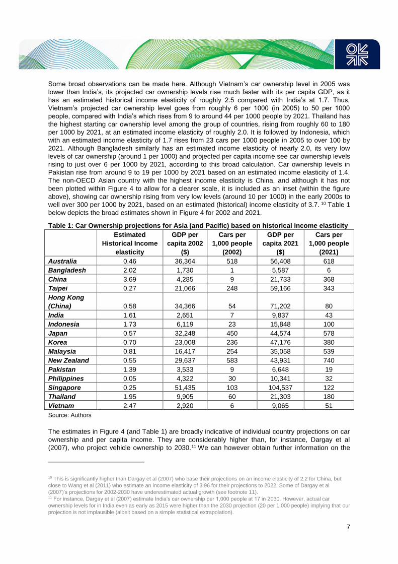
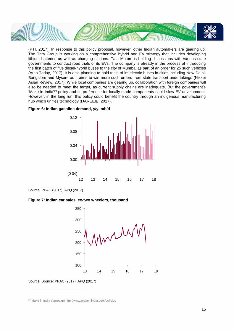
Figure 6: Indian gasoline demand, y/y, mb/d

Source: PPAC (2017); APQ (2017)

Figure 7: Indian car sales, ex-two wheelers, thousand

Source: Source: PPAC (2017); APQ (2017)

29 Make in India campaign http://www.makeinindia.com/policies

(0.04)

0.00

0.04

0.08

0.12

12 13 14 15 16 17 18

100

150

200

250

300

350

13 14 15 16 17 18

16

Implications for the power sector

While automakers prepare to meet the challenge of new vehicle demand, the power sector also

needs to gear up, by building capacity as well as improving plant load factors and distribution

networks. India has 330 GW of installed generating capacity consisting of 57 GW of renewables and

198 GW of thermal (Sen, 2017). Assuming an electric vehicle has a 100 KWh battery size, the annual

additional power demand for 6 million EVs is expected to be 93 TWh, which would require 10 GW of

power plant capacity in 2020. According to our estimates 2 million EVs would take roughly 3 GW of

power plant capacity, which represents 1% of installed capacity (EY, 2016; APQ, 2017).

While the country is likely to have sufficient power capacity to meet incremental demand from EVs, it

will need to overcome a number of structural challenges that are keeping power capacity at low

utilisation rates. Despite abundant coal resources, development has been stymied by bureaucratic

hurdles around various ministries and permits for land acquisition (Cornot-Gandolphe, 2016).

Feedstock sourcing, especially for natural gas, will be a limiting factor given the rising need for

imports alongside import infrastructure constraints. Gas also cannot compete with coal in the power

sector at current electricity prices, unless there is an explicit disincentive to using coal (such as a

carbon tax).30 The reliance on hydro resources has also left the country dependent on reservoir levels

during peak demand periods, often resulting in power cuts. Distribution infrastructure is inefficient with

large transmission losses, and power theft is perennial, deterring private investments while leaving

state utilities with poor finances that restrict their capacity to upgrade (Sen et al. 2016). Current power

capacity is largely underutilized despite urban areas facing erratic power cuts and the country aiming

to electrify more rural areas (Prasad, 2017). This implies that upcoming power capacity projects have

already been earmarked for solving current challenges. Additional stress on the power grid from EVs

will require a revamp of the sector to improve efficiencies at current power plants as well as the

distribution network.

Policy makers could, however, come around to seeing the utility in EVs not only for transportation but

also for its benefits to the power sector. For the power sector, EVs offer an opportunity to encourage

distributed generation, reducing dependence on electricity distribution companies (Discoms) and

setting up commercially sustainable micro grids, especially in remote areas. Batteries used in EVs

usually have a vehicle lifetime of 8-10 years, but they have significant potential after that for

alternative uses, especially as cheap storage for renewable energy capacity. It also helps improve

utilisation of existing domestic coal capacity by providing demand assurance to sustain a certain

baseload. Plant load factors have declined from 77% in 2010 to less than 60% currently (Prasad,

2017). With most of the charging expected to be done during off-peak hours, utilities can better

manage their base load rather than rely on expensive sources for generating peak load. India’s

largest power generation utility (NTPC) is looking to set up charging stations, with plans to halve the

cost of setting up these charging stations to $1,500 each, as a way to expand its market (PV

Magazine, 2017).

There is thus scope for baseload management at current capacity to improve plant load factors to

over 70% and more, to absorb the strain of millions of EVs on the power grid. In order for the EV push

to also conform with India’s COP21 commitments, electricity will need to be generated from

renewables, of which the government plans to generate 175 GW by 2022 (100 GW will be from solar

power).

While the power sector can accommodate the expansion of EVs by improving utilisation rates, the

biggest infrastructure challenge comes from expanding the charging infrastructure. While plug-in

sockets at household and commercial centres can be used, ultimately the infrastructure required to

charge EVs and lorries within a few minutes would have to be built from scratch. The challenge with

30 See Sen (2017) for details.

17

expanding the retail fuel network has been the dearth of reliable power supply in small towns and

remote highways. If such fuel stations were also to meet the demand of charging EVs, during power

cuts and low voltage periods the owners would have to set up generators. To incentivise the build out

of charging stations, the government is considering using a private retail method, using the same

model for distributed charging as was the case for privately-owned phone booths, implying that

anyone could set up a charging station and earn a small income from it.

Policy measures to enable EV penetration

The up-front price of the vehicle is likely to be a limiting factor, as they currently cost more than those

based on internal combustion engines (Shakti, 2017). That said, several measures are being

considered that could reduce the initial cost of buying an EV. For the individual user, the initial cost of

buying EVs can be brought down by as much as 50% if EVs are sold without batteries which will then

be swapped out rather than embedded (NITI Aayog, 2017). One option being considered is to allow

drivers to buy the car and lease the battery, which they can switch when they need to recharge

(Froese, 2017).

In order to build scale rapidly, India’s government is considering rolling out an EV-based public

transport system with auto-rickshaws and buses sold with batteries that can be swapped after a

certain distance (QI, 2017). Auto-rickshaws, for instance, travel between 80 km and 130 km daily, so

batteries could, in theory, be swapped at around the 40 km-mark (QI, 2017). A swappable battery

system is also an alternative being considered for city buses. With close to 95% of buses in the

country traveling 30 km per trip routes, batteries can be swapped at the terminal point where the bus

turns around for the return journey (QI, 2017). While this solves the challenge of having charging

stations that need to charge the batteries rapidly, as well as the cost of buying an electric vehicle for

the user, it would still require considerable investment to set up a battery swapping station, as well as

a convergence in technology across the industry, which is a challenge that will have to be overcome

with the right incentives for the sector, but it is possible to achieve. Adopting a shared ownership

model over an individual ownership model could bring down the cost of both ownership and travel.

India’s ride hailing companies are also partnering with manufacturers to grow its fleet (e.g. Ola with

Mahindra) by offering discounts on the cars, vehicle financing and maintenance plans to drivers (ET

Auto, 2017).

Currently, India has roughly 31 million passenger cars and 150 million two and three-wheeler

vehicles. The country consumes an average of 0.5 mb/d of gasoline and 1.56 mb/d of diesel. The

current target of 6 million EVs by 2020, if realised, could potentially displace roughly 90,000 b/d of fuel

demand in the country (APQ, 2017). Given the charging infrastructure limitations, and the challenges

of ramping up domestic manufacturing, a lower achievement of say 2 million EVs is more likely, and

would displace around 30,000 b/d of fuel demand (APQ, 2017). In the near term, EVs are unlikely to

be big disruptors to an otherwise steady gasoline demand story, with growth set to rise by 8-10%

year-on-year on average through 2020. It is the post-2020 timeframe where EV adoption is likely to

pick up pace, once charging infrastructure grows. The impact on fuel demand could be large if

commercial vehicles such as trucks are also electrified. The Indian government has already set in

motion efforts to electrify the diesel-dependent railways, which will lead to further displacement of fuel.

4.2 China – Implications of New Energy Vehicles and Fuel Efficiency

Unlike India, China’s ambitious efforts to tackle tailpipe emissions are already starting to slow

gasoline demand growth, but the government’s measures go beyond EVs to include policies to raise

fuel efficiencies in internal combustion engine vehicles, promoting use of hybrid vehicles, as well as

natural gas vehicles (NGVs). Even the advent of bike sharing apps is chipping away at gasoline

demand growth. Already in 2017, China’s gasoline demand growth is expected to slow to 0.11 mb/d

(3.5%), almost half of the 2016 growth rate (SCMP, 2017), as incremental car sales slow from over

18

13% in 2016 (China Daily, 2017b) to 5%31 at best in 2017, and alternative energy vehicles begin to

chip away at demand growth. Going forward, EVs alone could displace 45,000 to 55,000 b/d of

demand growth, with measures to increase fuel efficiencies knocking off even higher volumes. In

other words, had Chinese gasoline demand growth maintained the average growth rates seen

between 2011 and 2015 (0.23 mb/d, or 11%), the country would have consumed an additional 0.25-

0.30 mb/d of gasoline every year through 2020. At current rates, however, with car sales slowing,

efficiency gains rising and new energy vehicle sales rising, demand growth could average 0.15-0.20

mb/d through 2020 (APQ, 2017).

New Energy Vehicle (NEV) Plan and Impact on Gasoline Demand

The country’s NEV plan—which includes plug-ins, EVs and gas-fired vehicles—was rolled out in 2012

with goals through to 2020 (China State Council, 2012), and after some teething pains is now

increasingly starting to gain traction. China’s electric car fleet is dwarfed by conventional cars; last

year’s sales of the latter were more than 25 times the country’s entire electric car fleet. Electric cars

make up 0.5% of China’s fleet and the effects on fuel demand patterns are still marginal. Yet China’s

NEV push meets three distinct goals. First, to reduce some of the country’s hefty oil import bill and

enhance energy security (Zheng, 2017). Second, it should support the country’s environmental goals,

though as in India, it will require substantial progress on plans for renewables to take up a growing

share of power generation given the predominance of coal in the energy mix. Third, NEVs are also

part of the ‘Made in China 2025’ programme, China’s industrial upgrading plan (SCC, 2015). This goal

resonates with China’s carmakers, the majority of which see this as an opportunity to leapfrog their

western competitors.

Figure 8: China NEV sales, thousand units

Source: CAAM, Energy Aspects analysis, APQ (2017)

31 According to the China Association of Automobile Manufactures (CAAM), cited in China Daily (2017b).

0

20

40

60

80

100

120

140

Jan 15 Jul 15 Jan 16 Jul 16 Jan 17 Jul 17

19

Figure 9: China car sales, million units

Source: CAAM, Energy Aspects analysis, APQ (2017)

By 2020, Beijing plans to have 5 million NEVs on the road. This target includes 4.3 million passenger

vehicles, around 0.3 million taxis, 0.2 million buses and 0.2 million special vehicles. The ‘Made in

China 2025’ programme also highlights infrastructure development: it aims to install 4.3 million private

charging outlets (essentially one charger par car) and 0.5 million public chargers for cars, 4,000

charging stations for buses, 2,500 for taxis, 2,500 for special vehicles and about 2,400 city public

charging stations. At the end of 2016, China had 1 million EVs and 150,000 charging stations, or one

for every seven cars. The government is aiming to add another 100,000 charging stations by the end

of 2017 (IEA, 2016).

Issuing a plan is not enough, though. To encourage EV sales, China’s Ministry of Finance has been

providing subsidies ranging from RMB 30,000 to 60,000 ($4,400-8,800) for electric passenger

vehicles and subsidies of RMB 500-600,000 ($74,000-88,000) for commercial vehicles (MoF, 2015),

most of which are also matched by provincial governments. Local subsidies vary significantly as they

tend to favour local carmakers. The city of Beijing, for example, is home to Beijing Automotive

Industry Corp (BAIC), which makes pure electric cars, so Beijing city offers high subsidies for pure

electrics but no subsidies at all for plug-in hybrids. By contrast, Shanghai provides generous subsidies

for plug-in hybrids, largely because the Shanghai government owns SAIC, which makes that type of

vehicle. Localities therefore have a substantial say in NEV penetration rates and tailor their subsidies

to fit only locally made cars, or direct city governments to purchase locally made electric cars for their

fleets.

The central government has also waived sales tax and license taxes for EVs. Indeed, several of

China’s major metropolitan areas control the growth of their vehicle population in order to limit traffic

congestion by employing a license lottery or auction system, from which EVs are generally excluded.

In Beijing, EVs are also excluded from driving restrictions on heavily polluted days, making them

increasingly appealing to local drivers. And in order to support domestic industry, the government

scrapped a purchase tax on locally produced NEVs. On the supply side, the government has

introduced multiple R&D programmes to promote battery technology development, and has been

encouraging charging infrastructure development (MoF, 2016; IEA, 2016). These measures have

helped accelerate adoption rates: from total production of just over 8,000 five years ago, new electric

0.0

0.5

1.0

1.5

2.0

2.5

3.0

13 14 15 16 17 18

20

vehicle production in China grew to nearly half a million by 2015 with sales reaching 450,000. In 2016,

that number surged again by 53% y/y to 507,000 units sold.32

At the same time, the government’s generous subsidies led over 200 Chinese companies to enter the

NEV space, some of which have been happy to take subsidies without producing commercially viable

vehicles. In September 2016, the Chinese government fined five manufacturers that collected over

$120 million in subsidies but either failed to produce the vehicles, or sold vehicles with lower battery

ranges than the models they received the subsidies for. The government subsequently launched a

nation-wide investigation (Cui et al, 2017) and reviewed its subsidy scheme, leading it to slash

subsidies by 20% in January 2017 and plan to phase them out completely by 2020 (Cui et al, 2017).

After the government cut subsidies, NEV sales plummeted in January 2017, compared to a 132% y/y

increase in January 2016, but recovered in subsequent months. In May 2017, NEV sales totalled

45,000, up 28.4% y/y, while 51,000 NEVs were produced, a 38% y/y increase.33 These growth rates

have slowed compared to 2016 and could continue to decelerate as subsidies are phased out, but the

government is currently drafting new regulations which will also include a requirement that EVs

account for 8% of total car sales, perhaps as soon as 2018, and 12% by 2020 (Bloomberg, 2017).

Automakers that fall short of their production quotas can import EVs, or purchase credits from other

EV makers. While the aim is to encourage EV production with both carrots and sticks, following the

large subsidy scandals, Beijing is also looking to cut the number of players down to just 10. Those

that survive the cull will benefit from subsidies designed to nurture a competitive domestic industry

and create a vibrant consumer market for new energy vehicles. In addition, sales of low-speed electric

vehicles (LSEV: an indigenous Chinese innovation that looks a lot like an electric golf cart, used

traditionally in rural China) have also grown considerably from under 100,000 in 2010 to 600,000 in

2015, skyrocketing to almost 1 million vehicles in 2016, because of their small size, cheap price and

the fact that they can be driven without a license. Although initially popular in rural China, LSEVs have

become common in China’s third and fourth tier cities and are increasingly making inroads into the

country’s larger cities as an energy efficient alternative to traditional gasoline fired cars, public

transportation and two-wheelers. That said, the lack of regulations on LSEV production and sales as

well as rising safety concerns associated both with driving them and with the disposal of the lead-acid

batteries will likely prompt the government to tighten oversight over LSEVs (IEA, 2016). This could

lead to a slowdown in sales growth, but auto industry sources in China still expect sales to reach 2

million by 2020. Even though NEVs will not transform fuel demand patterns, they could shave off an

estimated 40,000 to 50,000 b/d of gasoline demand by 2020 (APQ, 2017).

At the same time, NEVs—large or small—are only part of the reason for the softness in gasoline

demand growth seen in 2017-to-date: the rise of electric buses and two-wheelers are further slowing

gains in gasoline demand growth. China currently has an estimated stock of over 200 million electric

two-wheelers, following a rapid uptick when conventional two-wheelers were banned in several cities

in order to reduce local pollution. Electric bike sales began modestly in the 1990s and started to take

off in 2004, when 40,000 were sold. In late 2016, that number had reached 20 million. China is also

leading the global deployment of electric bus fleets, with more than 170,000 buses already circulating

today.

That said, a number of challenges remain: Chinese battery technology is relatively weak and the

driving range for Chinese models, despite significant improvements, remains lower than Western

carmakers, while charging times are still longer. Second, battery costs remain high and the

fragmented nature of the Chinese automotive industry discourages economies of scale in R&D. The

hefty subsidies currently in place reduce the urgency for carmakers to cut battery costs, but as the

government begins to phase out subsidies, failure to trim expenses could impede EV penetration into

the Chinese car fleet. Third, even though Beijing is focusing increasingly on infrastructure

32 According to CAAM. 33 Ibid.

21

development, regulatory approvals for land acquisition or facility installation in residential compounds

could slow the infrastructure rollout and increase the costs associated with it.

Nonetheless, even though the government may fail to reach its 5-million-unit target in 2020, NEVs will

become a larger component of the Chinese car fleet and will slow demand growth for gasoline. CNPC

estimates that in 2015, NEVs shaved off roughly 80,000 b/d of gasoline demand and according to

government estimates, by 2020 NEVs will displace 0.3-0.4 mb/d of gasoline demand (CSD, 2017).

Impact of higher fuel efficiencies, NGVs and bike-sharing

The biggest factor for gasoline demand, however, is fuel efficiency targets. Beijing has set out

ambitious targets for reducing average fuel consumption from 6.9 litre/100km in 2015 to 5.0

litre/100km in 2020. In 2016, domestic passenger vehicle manufacturers claimed to have reached an

average of 6.95 litre/100km and after including credits from NEV production, the average fuel

consumption decreased to 6.6 litre/100km, suggesting that the government is on track to meet its goal

(ICET, 2016). If these fuel efficiencies continue to be rolled out, they will be key in reducing gasoline

demand growth—potentially displacing 50,000 to 80,000 b/d (with even further upside depending on

the efficiencies implemented as well as the overall miles driven in the country) (APQ, 2017).34

Beijing has equally ambitious targets for natural-gas vehicles (NGVs). The government is looking to

increase the number of NGVs in China from 5.2 million in 2015 to 10.5 million units by 2020. NGVs

have already benefitted from government support, including production subsidies as well as R&D

funding for technology development. Highway tolls are also waived for NGVs. But there are a number

of constraints to promoting NGVs more rapidly. First, as demand growth is recovering, natural gas

supplies are failing to keep up and are prioritised for industrial and residential use. Second, major gas

producing regions such as Shandong, Xinjiang, and Sichuan, boast high levels of NGVs—the three

provinces combined account for more than half of China’s NGVs—as they can supply gas for

transportation at close to well-head price, but in other potential consumer hubs, especially along

China’s coastal provinces where air pollution is at its most severe, prices for natural gas in

transportation are higher (Hao et al, 2016). Moreover, the priority for natural gas in these provinces is

phasing out coal-fired boilers so gas in transport will have a less prominent role. As more coal use is

phased out through late 2017 and early 2018, incremental supplies in these provinces could start

going into the transportation sector.

Finally, bike sharing apps are also denting gasoline demand growth. This latest craze picked up in

mid-2016 and has since brought more than 2 million bikes to city streets, operated by around 30

companies. These rival companies offer bikes—at steep discounts as they compete for market

share—around China’s largest cities that can be unlocked using mobile apps. But unlike similar

initiatives around the world, bikes can be picked up and left anywhere by scanning a QR code on the

frame, making them convenient for users, even though the piles of bikes left around the city has

frustrated the authorities (Horwitz, 2017). An estimated 20 million people used these bike-share

schemes in 2016 and that figure is expected to reach over 200 million by 2020, according to a report

by research firm Research and Markets. There are some 30 operators deploying bike-sharing

services since mid-2016. In light of the rapid expansion, large municipalities such as Beijing and

Shanghai are tightening regulations over bike sharing, especially on parking standards (Jaganathan

and Tan, 2017; Yifan, 2017).

All these measures combined start to affect China’s gasoline demand patterns even though in a fleet

of over 200 million conventional vehicles, the impact of 5 million units is extremely limited. The

country’s gasoline demand at 3.1 mb/d may still rise to around 3.6 mb/d in 2020 (APQ, 2017). Had the

country continued on its 2011-2015 path, of 11% average growth rates, it would be adding around

0.25-0.30 mb/d of demand each year. But with NEVs denting demand at the margins and fuel

34 Energy Aspects estimates.

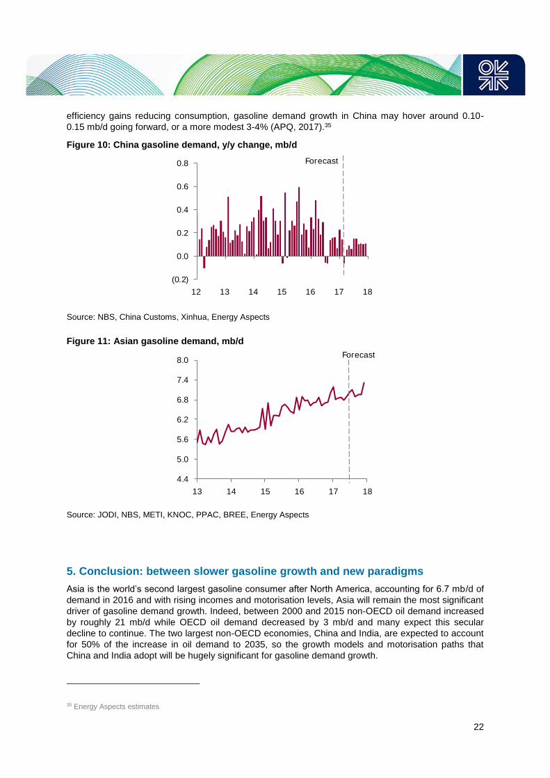
22

efficiency gains reducing consumption, gasoline demand growth in China may hover around 0.10-

0.15 mb/d going forward, or a more modest 3-4% (APQ, 2017).35

Figure 10: China gasoline demand, y/y change, mb/d

Source: NBS, China Customs, Xinhua, Energy Aspects

Figure 11: Asian gasoline demand, mb/d

Source: JODI, NBS, METI, KNOC, PPAC, BREE, Energy Aspects

5. Conclusion: between slower gasoline growth and new paradigms

Asia is the world’s second largest gasoline consumer after North America, accounting for 6.7 mb/d of

demand in 2016 and with rising incomes and motorisation levels, Asia will remain the most significant

driver of gasoline demand growth. Indeed, between 2000 and 2015 non-OECD oil demand increased

by roughly 21 mb/d while OECD oil demand decreased by 3 mb/d and many expect this secular

decline to continue. The two largest non-OECD economies, China and India, are expected to account

for 50% of the increase in oil demand to 2035, so the growth models and motorisation paths that

China and India adopt will be hugely significant for gasoline demand growth.

35 Energy Aspects estimates

(0.2)

0.0

0.2

0.4

0.6

0.8

12 13 14 15 16 17 18

Forecast

4.4

5.0

5.6

6.2

6.8

7.4

8.0

13 14 15 16 17 18

Forecast

23

This paper investigated the following research questions: first, what are the key drivers of gasoline

demand growth in non-OECD Asia, based on historical trends? And second, what are the constraints

to gasoline demand growth in this region? The first question, driven by historical trends, was

investigated using statistical analyses on a panel dataset of 19 countries in the Asia-Pacific region, of

which over half are non-OECD countries. The dynamic specification of our model suggested that on

average a 1% increase in vehicle ownership could potentially lead to a 25% increase in gasoline

consumption – but this result needs to be strongly qualified by the fact that the statistical analysis

does not account for country-specific policy interventions which could change the outcome. Results

from the statistical analysis also confirmed that income and vehicle ownership are the key drivers of

gasoline consumption in non-OECD Asia. When looking solely at the income elasticity of car

ownership alongside GDP and population, our results suggested that car ownership in Asia could

plateau at lower levels than in OECD countries, at around 400 cars per 1000 people, roughly half of

the US model (800 cars per 1000 people). Our case studies showed that China and India are both

charting different courses. Both have seen rising oil imports take a toll on their foreign exchange

reserves, and the need to tackle poor air quality is leading them to substitute traditional vehicles and

improve efficiencies. While India’s efforts may only begin to displace around 15,000 to 20,000 b/d of

gasoline demand around 2020, China’s policies to encourage NEV penetration, combined with more

stringent fuel economy standards, are already slowing demand growth, displacing around 0.1-0.15

mb/d of gasoline demand every year.

If we return to the three potential arguments set out in Section 1, it is evident that policy constraints on

gasoline demand growth, while in many cases initiated at the regional or city level, are being

consolidated at the national level. While these economies are entering or are already in high growth

trajectories with car ownership levels rising, oil demand growth in transport is likely to slow relative to

a baseline as policies to substitute away from oil in transport are implemented on a widespread basis

and backed by strong political commitment. Oil demand growth could slow further if battery

technologies improve rapidly and costs come down, and if these countries transition to different

mobility models with ride sharing gaining prominence – causing rapid and disruptive change in

transport. Displacement of gasoline consumption will then be even higher—especially in India after

2020.

24

References

APQ (2017) ‘Driving Asia’s Gasoline Demand’, Asia-Pacific Quarterly, pp. 5-23, Energy Aspects.

Auto Today (2017) ‘Tata Motors launches electric hybrid buses priced up to Rs. 2 crore,’ 25 January

[Available at http://indiatoday.intoday.in/auto/story/tata-motors-launches-electric-hybrid-buses-priced-

up-to-rs-2-crore/1/866223.html]

Baum, C.F. (2006). An Introduction to Modern Econometrics Using Stata. College Station, TX: Stata

Press.

Becker, Gary S. (1965) ‘A theory of the allocation of time’, Economic Journal, 75, 493– 517.

Bloomberg (2017) ‘China Revises EV Credit Points to Reward Longer-Range Models’, Bloomberg

News, 13 June. [Available at https://www.bloomberg.com/news/articles/2017-06-13/china-tweaks-

proposed-ev-formula-to-reward-longer-range-models-j3v68b09]

BP (2016) BP Energy Outlook 2016 Edition.

BP (2017) BP Energy Outlook 2017 Edition.

Bun, M.J G. and Kiviet, J.F. (2003). ‘On the diminishing returns of higher-order terms in asymptotic

expansions of bias’. Economics Letters, 79(2), pp. 145-152.

Button, Kenneth, Ndoh Ngoe, and John Hine (1993). “Modeling Vehicle Ownership and Use in Low

Income Countries.” Journal of Transport Economics and Policy. January: 51-67.

China Daily (2017a) ‘China 2016 car sales surge at fastest rate in three years’, South China Morning

Post, 12 January. [Available at http://www.scmp.com/business/china-business/article/2061642/china-

2016-car-sales-surge-fastest-rate-three-years]

China Daily (2017b) “July car sales hit five month low”, China Daily, 14 August. [Available at

http://www.chinadaily.com.cn/business/motoring/2017-08/14/content_30573571.htm]

China State Council (2012) China State Council, “Energy saving and new energy vehicles industry

development planning (2012-2020)”. [Available at http://www.gov.cn/zwgk/2012-

07/09/content_2179032.htm] (Chinese)

CSD (2017) A ban on traditional vehicles is now on the agenda”, 14 September, China Securities

Daily, [Available at http://energy.people.com.cn/n1/2017/0914/c71661-29534908.html]

Cornot-Gandolphe, S. (2016) ‘Indian Steam Coal Imports: The Great Equation’, OIES Paper CL3,

Oxford Institute for Energy Studies. https://doi.org/10.26889/9781784670528

Cui, H. Yang, Z. and He, H. (2017) ‘Adjustment to subsidies for new energy vehicles in China’, ICCT

policy update, 17 May [Available at http://www.theicct.org/publications/adjustment-subsidies-new-

energy-vehicles-china].

Dargay, J., Gately, D., and Sommer, M. (2007). ‘Vehicle Ownership and Income Growth, Worldwide:

1960–2030’,The Energy Journal, 28 (4), 143–70.

Dargay, Joyce (2001). “The effect of income on car ownership: evidence of asymmetry”,

Transportation Research, Part A. 35:807-821.

Dargay, J., and Gately, D. (1999). ‘Income’s effect on car and vehicle ownership, worldwide: 1960–

2015’, Transportation Research, Part A, 33: 101–38.

de Jong, G., Fox, J. Pieters, M., Daly, A.J. and Smit, R. (2004) ‘A Comparison of Car Ownership

Models’, Transport Reviews, 24 (4), 397-408.

25

Eskeland, G., and T. Feyzioglu (1997), ‘Rationing can backfire: The "day without a car" in Mexico

City’, World Bank Economic Review, 11, 383-408.

ET Auto (2017) ‘Ola, Mahindra partners with governments to build electric mobility system in Nagpur’,

ET Auto, 26 May. [Available at https://auto.economictimes.indiatimes.com/news/industry/ola-

mahindra-partners-with-govt-to-build-electric-mobility-system-in-nagpur/58860040].

EY (2016) ‘Electric vehicles adoption: potential impact in India’, EY. [Available at

http://www.ey.com/Publication/vwLUAssets/EY-ev-adoption-potential-impact-in-India-july-

2016/$FILE/EY-ev-adoption-potential-impact-in-India-july-2016.pdf]

Froese, M. (2017) ‘Plug-in EVs: Future market conditions and adoption rates’, Windpower

Engineering Development, 24 October. [Available at

http://www.windpowerengineering.com/electrical/plug-evs-future-market-conditions-adoption-rates/]

Hall, A.R. (2005). Generalized Method of Moments. Oxford: Oxford University Press.

Hao, H., Liu, Z., Zhao, F. and Li, W. (2016) ‘Natural gas as vehicle fuel in China: A review’,

Renewable and Sustainable Energy Reviews, Vol 62, September, pp 521-33.

HBL (2015) ‘Modi calls for slashing oil, gas imports by 10% in next 7 years’ Hindu Business Line, 27

March [Available at http://www.thehindubusinessline.com/economy/pm-says-india-should-try-to-cut-

oil-imports-by-10-in-2022/article7039287.ece]

Horwitz, J. (2017) ‘China’s cities are saying “enough already” to bike sharing services run rampant’,

Quartz, 22 August. [Available at https://qz.com/1058438/chinese-cities-saying-enough-already-to-

chaos-generated-by-bike-sharing-services-like-ofo-and-mobike/]

HT (2017) ‘India, China vie to tap clean energy market by phasing out fossil-fuel vehicles’, Hindustan

Times, 3 October. [Available at http://www.hindustantimes.com/india-news/india-china-vie-to-tap-

clean-energy-market-by-phasing-out-fossil-fuel-vehicles/story-jjvrxOo3FTDk0DpR6jo0YO.html]

Huo, H., Wang, M., Johnson, L. and Dongquan, H. (2007) ‘Projection of Chinese Motor Vehicle

Growth, Oil Demand, and CO2 Emissions through 2050’, Transportation Research Record: Journal of

the Transportation Research Board, Volume 2038.

Huo, H. and Wang, M. (2012) ‘Modelling future vehicle sales and stock in China’, Energy Policy, Vol.

43, pp.17-29.

ICET (2016) China Passenger Vehicle Fuel Consumption Development Annual Report 2016, The

Innovation Center for Energy and Transportation, September. [Available at

http://www.icet.org.cn/english/admin/upload/2016092735417005.pdf]

IBP (2015) Brunei Energy Policy, Laws and Regulations Handbook, International Business

Publications, USA.

ICCT (2016) ‘Hybrid and Electric Vehicles in India: Current Scenario and Market Incentives’, the

International Council on Clean Transportation. [Available at

http://www.theicct.org/sites/default/files/publications/India-hybrid-and-EV-incentives_working-

paper_ICCT_27122016.pdf].

IEA (2015) World Energy Outlook, International Energy Agency, Paris.

IEA (2016) Global EV outlook 2016: Beyond one million electric cars, Paris: OECD/IEA 2016

IJAREEIE (2017) ‘Alternative Energy Based Electric Vehicle Charging Station’, International Journal

of Advanced Research in Electrical, Electronics and Instrumentation Engineering; Vol. 3 Issue 6.

[Available at https://www.rroij.com/open-access/alternative-energy-based-electric-vehicle-charging-

station-.pdf]

26

Ingram, G.K. and Liu, Z (1999) ‘Vehicles, Roads, and Road Use: Alternative Empirical Specifications’,

World Bank Policy Research Working Paper, World Bank, Washington.

Ingram, G.K. and Liu, Z (1997) ‘Motorization and Road Provision in Countries and Cities’, World Bank

Policy Research Working Paper WPS1842, World Bank, Washington.

Jaganathan, J. and Tan, F. (2017) “Two wheels good: Bike boom nibbles on Asia gasoline demand

growth”, Reuters, 26 September. [Available at https://www.reuters.com/article/us-asia-bicycles/two-

wheels-good-bike-boom-nibbles-on-asia-gasoline-demand-growth-idUSKCN1C10ZJ]

Judson, R.A. and A.L. Owen (1999). ‘Estimating Dynamic Panel Data Models: A Guide for

Macroeconomists’, Economics Letters, 65, pp. 9-15.

Kennedy, P. (2008). A Guide to Econometrics. Oxford, Blackwell Publishing.

Kiviet, J.F. (1995) ‘On Bias, Inconsistency, and Efficiency of Various Estimators in Dynamic Panel

Data Models’, Journal of Econometrics, 68 (1), pp. 53-78

Lancaster, K.J. (1966) ‘A new approach to consumer theory’, Journal of Political Economy, 74, 132–

157.

Medlock, K.B. III and Soligo, R. (2001) ‘Car Ownership and Economic Development with Forecasts to

the Year 2015’, Journal of Transport Economics and Policy, Vol. 36, No. 2 (May, 2002), pp. 163-188

Moavenzadeh, F. and Gletner, D (1984) ‘Transport, Energy and Economic Development’, Elsevier,

Amsterdam.

MoF (2015) Ministry of Finance, Notice on 2016-2020 fiscal subsidy policies on NEV promotion and

application. 2015. [Available at

http://jjs.mof.gov.cn/zhengwuxinxi/zhengcefagui/201504/t20150429_1224515.html]

MoF (2016). Ministry of Finance. “Notice on adjusting the fiscal subsidy policies on NEV promotion

and application”. [Available at

http://jjs.mof.gov.cn/zhengwuxinxi/tongzhigonggao/201612/t20161229_2508628.html]

Muth, R.F. (1966) ‘Household production and consumer demand functions’, Econometrica, 34, 699–

708.

Nielsen Global Survey of Automotive Demand (2013), Nielsen. [Available at

http://www.nielsen.com/ae/en/press-room/2014/nielsen-global-automotive-report.html]

Nikkei Asian Review (2017). ‘Tata Group ramps up electric vehicle strategy as India seeks to curb air

pollution’, Nikkei Asian Review, June 27. [Available at https://asia.nikkei.com/Business/AC/Tata-

Group-ramps-up-electric-vehicle-strategy-as-India-seeks-to-curb-air-pollution]

NITI Aayog (2017) ‘India Leaps Ahead: Transformative Mobility Solutions for All’, Government of

India. [Available at

http://niti.gov.in/writereaddata/files/document_publication/RMI_India_Report_web.pdf]

PPAC (2017) Consumption of Petroleum Products; Petroleum Planning and Analysis Cell;

Government of India. [Available at http://ppac.org.in/index.aspx].

Prasad, G.C. (2017) ‘Government planning liberal norms for electric vehicle charging stations’,

LiveMint, 21 October. [Available at http://www.livemint.com/Politics/Pii8GbSglucqIvIQqgG1SI/Govt-

planning-liberal-norms-for-electric-vehicle-charging-st.html].

PTI (2017) ‘Mahindra aims to increase electric vehicle production to 5,000 units per month by 2019’,

Press Trust of India; May 28. [Available at https://auto.ndtv.com/news/mahindra-aims-to-increase-

electric-vehicle-production-to-5000-units-per-month-by-2019-1704853]

27

PV Magazine (2017) ‘India’s NTPC set to enter EV charging station business’, PV Magazine, 24

October. [Available at https://www.pv-magazine.com/2017/10/24/indias-ntpc-set-to-enter-ev-charging-

stations-business/].

QI (2017) ‘India’s electric vehicle revolution will begin with autorickshaws running on swappable

batteries’, Quartz India, 9 June. [Available at https://qz.com/1001518/indias-electric-vehicle-

revolution-will-begin-with-auto-rickshaws-running-on-swappable-batteries/].

SCC (2015) State Council of China, ~Made in China 2025, 2015 [Available at

http://www.gov.cn/zheng ce/content/2015- 05/19/content_9784.htm]

SCMP (2017) ‘China 2016 car sales surge at fastest rate in three years’, South China Morning Post,

12 January, [Available at http://www.scmp.com/business/china-business/article/2061642/china-2016-

car-sales-surge-fastest-rate-three-years]

Sen, A. and Sen, A. (2016) ‘India’s Oil Demand: On the Verge of Take-off?’ OIES Paper WPM 65,

Oxford Institute for Energy Studies. https://doi.org/10.26889/9781784670535

Sen, A., Nepal, R., and Jamasb, T. (2016) ‘Reforming Electricity Reforms? Empirical Evidence from

Asian Economies’, OIES Paper EL18, Oxford Institute for Energy Studies.

https://doi.org/10.26889/9781784670504

Sen, A. (2017) ‘India’s Gas Market Post-COP21’, OIES Paper NG120, Oxford Institute for Energy

Studies. https://doi.org/10.26889/9781784670863

Shakti (2017) ‘Dispelling Myths: Electric Vehicles will be Expensive and a Burden on the Indian

Electricity Grid’, Shakti Sustainable Energy Foundation [Available at http://shaktifoundation.in/wp-

content/uploads/2014/02/Myth-Buster-Electric-Vehicles-September-2017.pdf]

Storchmann, K. (2005) ‘Long-Run Gasoline demand for passenger cars: the role of income

distribution’, Energy Economics, 27, 25-28.

Wang, Y., Teter, J. and Sperling, D. (2011) ‘China’s sparing vehicle population: even greater than

forecasted?’ Energy Policy 39, pp. 3296-3306.

WEC (2016) World Energy Resources 2016, World Energy Council. [Available at

https://www.worldenergy.org/wp-content/uploads/2016/10/World-Energy-Resources-Full-report-

2016.10.03.pdf]

Yifan, G. (2017), “Industry Observer: Where has China’s gasoline demand growth gone?” Financial

News Daily, 13 July. [Available at http://futures.jrj.com.cn/2017/07/13074522741334.shtml ](Chinese)

Zheng, L. (2017) “Review of CO2 emissions cutbacks with Electric Vehicles in China”, IEEJ, April

2017. [Available at https://eneken.ieej.or.jp/data/7259.pdf]

28

Appendices

A. Data Sources

Data was obtained from the International Road Federation Statistics, World Bank World Development

Indicators, ASEAN Statistical Database, UNESCAP Database, UN Population Statistics, Energy

Aspects, International Organization of Motor Vehicle Manufacturers, and country-specific statistical

divisions where necessary.

B. Descriptive Statistics

Variable Name Var. Label Mean SD Min Max

Gasoline Consumption (b/d) gdd 246.7008 418.0532 .9153005 2669.905 Gasoline Cons. Per Capita (Bbls) gddpc 1.543749 1.775675 .0160921 6.270487 Fuel Price (US$/bbl) price 78.55291 27.90167 32.96797 117.2294 Per Capita Income (US$) gdppc 22714.19 22122.47 656.5597 80192 Vehicle Ownership (cars/’000) vo 182.7467 205.2189 .99466 638.6898 Total Vehicles vtot 1.08e+07 1.85e+07 77000 1.16e+08 Vehicle Ownership Per Capita vopc .1827467 .2052189 .0009947 .6386898 Road Density (Kms/1,000km2) rden 1250.278 2415.168 43 14080 Share of Manufacturing in GDP (%) gdpman 19.30533 7.90537 1.283804 32.718 Population pop 1.92e+08 3.75e+08 346000 1.40e+09 Urban Population urpop 8.18e+07 1.55e+08 250000 7.79e+08 Road Length (kms) rdl 594829.1 1237639 1943 5231922 Road Length Per Capita (kms) rdlpc .0048348 .0088344 .0001343 .0411939

N 266

C. List of Countries

OECD Non-OECD

Australia Bangladesh

Brunei China

Chinese Taipei/Taiwan India

Hong Kong China Indonesia

Japan Malaysia

South Korea Myanmar

Singapore Pakistan

New Zealand Papua New Guinea

Philippines

Thailand

Vietnam

29

D. Correlation Matrix

gdd gddpc price gdppc vo vtot vopc rden lrden gdpman pop urpop rdl rdlpc

gdd 1 gddpc -0.0223 1 price 0.0512 0.0425 1 gdppc -0.155 0.627*** 0.168* 1 vo 0.0513 0.906*** 0.0622 0.486*** 1 vtot 0.922*** 0.0531 0.128 -0.0668 0.190* 1 vopc 0.0513 0.906*** 0.0622 0.486*** 1 0.190* 1 rden -0.135 0.0463 0.102 0.324*** -0.00120 -0.118 -0.00120 1 lrden -0.116 -0.111 0.0780 0.387*** -0.109 -0.0334 -0.109 0.744*** 1 gdpman 0.433*** -0.252** -0.0137 -0.246** -0.174* 0.326*** -0.174* 0.175* 0.0854 1 pop 0.664*** -0.355*** -0.0633 -0.408*** -0.356*** 0.501*** -0.356*** -0.134 -0.0235 0.317*** 1 urpop 0.817*** -0.302*** -0.0265 -0.357*** -0.288*** 0.649*** -0.288*** -0.146 -0.0597 0.401*** 0.966*** 1 rdl 0.617*** -0.214** 0.00412 -0.312*** -0.212** 0.527*** -0.212** -0.123 -0.0106 0.189* 0.947*** 0.893*** 1 rdlpc 0.00917 0.810*** -0.0353 0.274*** 0.769*** 0.0141 0.769*** -0.192* -0.378*** -0.353*** -0.153 -0.142 0.0128 1

* p < 0.05, ** p < 0.01, *** p < 0.001

E. Postestimation Tests

Test of Endogeneity

H0: Variables are Exogenous

Models 1 & 2: GMM ‘C’ statistic chi2(1) = 42.6183 (p-value = 0.0000)

[H0 rejected]

Models 3 & 4: GMM ‘C’ statistic chi2(1) = 7.92765 (p-value = 0.0049)

[H0 rejected]

No overidentifying restrictions.

30

F. Econometric Method

The starting point for analysis in panel data techniques is to look at Least Squares Dummy Variable

(LSDV) estimators. However, LSDV performs well only when T is adequately large; with 30 years

suggested as a minimum threshold (Judson and Owen, 1999). Kiviet (1995) devised a bias-corrected

LSDV estimator (LSDVC), later refined by Bun and Kiviet (2003), which is generally seen to have the

lowest RMSE36 for panels of all sizes; its applicability was, however, limited to balanced panels. A

version of the bias-corrected LSDV estimator (LSDVC) for unbalanced panels was developed by

Bruno (2005), which operates under two assumptions; first, it has a strictly exogenous selection rule,

and second, it classifies the error term it as an ‘unobserved white noise disturbance’ (Bruno, 2005).

The LSDVC estimator’s exogenous selection rule conflicts with our model specification which includes

endogenous regressors, as described in Section 3. A number of consistent Instrumental Variable

(IV)37 and Generalised Method of Moments (GMM)38 estimators have been proposed in the literature

as alternatives to the LSDV and LSDVC estimators, and we run our estimations using an

instrumented variable regression (STATA routine ivregress).39 This fits a regression of depvar on

varlist1 and varlist2, using varlistiv (along with varlist1) as instruments for varlist2. 40 It supports

estimation using generalised method of moments (GMM) estimators.

The model estimated under this routine is as follows:

𝑦𝑖 = 𝑌𝑖𝛽1 + 𝑥1𝑖𝛽2 + 𝑢𝑖 (Structural equation)

𝑌𝑖 = 𝑥1𝑖Π1 + 𝑥2𝑖Π2 + 𝑣𝑖 (First-stage equation)

Here, 𝑦𝑖 is the dependent variable for the ith observation, 𝑌𝑖 represents the endogenous regressors,

𝑥1𝑖 and 𝑥2𝑖 represent the instruments and 𝑢𝑖 and 𝑣𝑖 are zero-mean error terms, and the correlations

between 𝑢𝑖 and the elements of 𝑣𝑖 are presumably non-zero. In our estimation method, apart from any

additional exogenous variables that are specified, other exogenous variables that appear in the

regression equation are automatically included as instruments. The results are robust to

heteroscedasticity.

36 Root Mean Square Error. 37 Baum (2006). 38 Hall (2005). 39 The syntax for ivregress assumes that you want to fit one equation from a system of equations or an equation for which you

do not want to specify the functional form for the remaining equations of the system. An advantage of ivregress is that you can

fit one equation of a multiple-equation system without specifying the functional form of the remaining equations. 40 varlist1 and varlistiv are the exogenous variables, and varlist2 the endogenous variables.

31

G: Fractional Polynomial Prediction Plots41 on Gasoline Consumption per Capita

Per Capita Income: Asia-Pacific Per Capita Income: Non-OECD Asia

Per Capita Vehicle Ownership: Asia-Pacific Per Capita Vehicle Ownership: Non-OECD Asia

Per Capita Road Length: Asia-Pacific Per Capita Road Length: Non-OECD Asia

41 Calculates the prediction for yvar (gasoline consumption) based on the estimation of a fractional polynomial of xvar and plots

the resulting curve along the confidence interval of the mean; these plots are a tool for graphically estimating relationships

between variables.