gaston giordana and michael ziegelmeyer, central … debt burden and financial vulnerability in...
TRANSCRIPT
IFC-National Bank of Belgium Workshop on "Data needs and Statistics compilation for macroprudential analysis"
Brussels, Belgium, 18-19 May 2017
Household debt burden and financial vulnerability in Luxembourg1
Gaston Giordana and Michael Ziegelmeyer, Central Bank of Luxembourg
1 This paper was prepared for the meeting. The views expressed are those of the authors and do not necessarily reflect the views of the BIS, the IFC or the central banks and other institutions represented at the meeting.
Household debt burden and financial vulnerability in Luxembourg 1
Household debt burden and financial vulnerability in Luxembourg1
Gaston Giordana2 and Michael Ziegelmeyer3
Abstract
We construct debt burden indicators at the level of individual households and calculate the share of households that are financially vulnerable using Luxembourg survey data collected in 2010 and 2014. The share of households that were indebted declined from 58.3% in 2010 to 54.6% in 2014, but the median level of debt (among indebted households) increased by 22% to reach €89,800. This suggests that indebted households in 2014 carried a heavier burden than indebted households in 2010. However, among several debt burden indicators considered, only the debt-to-income ratio and the loan-to-value ratio of the outstanding stock registered a statistically significant increase. The median debt service-to-income ratio actually declined, mainly reflecting lower costs on non-mortgage debt. Using conventional thresholds to identify financially vulnerable households, we find that their share in the population of indebted households increased, although the change was only statistically significant when measured by the debt-to-income ratio. The different indicators of debt burden and financial vulnerability are highly correlated with several socio-economic characteristics, including age, gross income and net wealth. In particular, low income households have lower leverage and disadvantaged socio-economic groups (in terms of education, employment status and home-ownership status) tend to be less financially vulnerable. However, after controlling for other factors, low income or low wealth increase the probability of being identified as vulnerable.
Keywords: Household debt; Household financial vulnerability; Financial stability; HFCS; Household finance
JEL classification: D10, D14, G21
1 This paper should not be reported as representing the views of the Banque centrale du
Luxembourg (BCL) or the Eurosystem. The views expressed are those of the authors and may not be shared by other research staff or policymakers in the BCL, the Eurosystem or the Eurosystem Household Finance and Consumption Network. We give special thanks to Paolo Guarda. In addition, we would like to thank Anastasia Girshina, Abdelaziz Rouabah, Jean-Pierre Schoder, Cindy Veiga, and participants at a seminar at the BCL for useful comments.
2 Economics and Research Department, Banque centrale du Luxembourg. E-mail: [email protected], tel. +352 4774 4553, fax +352 4774 4920.
3 Economics and Research Department, Banque centrale du Luxembourg. E-mail: [email protected], tel. +352 4774 4566, fax +352 4774 4920.
2 Household debt burden and financial vulnerability in Luxembourg
Contents
Household debt burden and financial vulnerability in Luxembourg .................................. 1
1 Introduction ....................................................................................................................................... 3
2 Methodology and data ................................................................................................................. 4
3 Results .................................................................................................................................................. 7
3.1 Indebted households........................................................................................................... 7
3.2 Debt burden indicators....................................................................................................... 9
3.3 Linking debt burden and household characteristics ............................................. 10
3.4 Vulnerable households ..................................................................................................... 12
3.4.1 Single indicator approach ............................................................................. 12
3.4.2 Multiple indicator approach ......................................................................... 14
3.5 Linking vulnerability and household characteristics ............................................. 17
4 Conclusion ........................................................................................................................................ 20
5 References ........................................................................................................................................ 21

Household debt burden and financial vulnerability in Luxembourg 3
1 Introduction
Despite their relative wealth, Luxembourg households are generally more indebted than households in other European countries (HFCN, 2013). This emphasises the need for a detailed assessment of household debt sustainability in Luxembourg. During the global financial crisis mortgage defaults had consequences for financial stability around the world. Unsustainable household debt also contributed to deepening the economic consequences of systemic banking crises in certain European countries following the global financial crisis. More recently, in responding to the low inflation environment, the European Central Bank (ECB) took unprecedented monetary policy measures, which cut household borrowing costs in the euro area (EA).
More recently, the Luxembourg central bank drew attention to concerns regarding household financial vulnerability (BCL 2015, 2016, 2017).4,5 In particular, the latest financial stability reviews noted the substantial share of loans with a short mortgage rate fixation period, which are vulnerable to unexpected interest rate increases. They also noted that household debt was growing faster than the value of household assets, implying higher bank losses in case of default. However, this analysis is limited by its reliance on aggregate data and population averages. The picture drawn from the analysis of time series data can be enriched using detailed cross-sectional balance sheet data at the individual household level. In spite of that, our cross-sectional balance sheet data refers to 2010 and 2014 and is less timely than aggregate data.
This paper calculates household-level indicators of debt burden and identifies financially vulnerable households using the 1st and 2nd wave of the Luxembourg Household Finance and Consumption Survey (LU-HFCS). Our analysis extends work reported in BCL (2013) to include the 2nd wave of the LU-HFCS conducted in 2014, and aims to complement the BCL (2017) assessment of household financial vulnerability by studying survey data. In particular, we provide a detailed description of the distribution of debt burden indicators by household socio-economic characteristics. In addition, we investigate which characteristics are more closely linked to household financial vulnerability. In future research we plan to implement a household stress test using micro-simulation methods.
The evidence we provide draws a mixed picture on the changes of household indebtedness and financial vulnerability in Luxembourg across the two waves. In 2014, 54.6% of all resident households were indebted. These households are the reference population for the analysis in this paper. The share of indebted households actually fell by 3.8 percentage points (ppt) since 2010, but the level of debt in the typical household increased. The conditional mean of household total debt increased by 27% to reach € 178,400 (the conditional median increased by 22% to reach € 89,800). Among the debt burden indicators we study, there were increases in the median debt-to-asset ratio, the median loan-to-value ratio (of the outstanding stock) and the median debt-to-income ratio. However, these changes
4 See the Section 3 in the first chapter of Revue de Stabilité Financière 2015 (pages 17-25) and Box
1.1 in Revue de Stabilité Financière 2016 (pages 21-23).
5 The European Systemic Risk Board also addressed a warning to Luxembourg about residential real estate developments and their financial stability consequences (ESRB/2016/09).

4 Household debt burden and financial vulnerability in Luxembourg
are only statistically significant for the debt-to-income ratio and the loan-to-value ratio (of the outstanding stock). In contrast, the debt service-to-income ratio declined due to the low interest rate environment. This was mostly driven by lower debt service on non-mortgage debt.
Financially vulnerable households are identified following two alternative approaches. The first approach considers one debt burden indicator at a time. This approach does not indicate a uniform significant increase in the share of financially vulnerable households between 2010 and 2014. The second approach combines information from several debt burden indicators and shows a larger (in relative terms) but still not statistically significant increase. The share of financially vulnerable households is 2.2% of the indebted population and 2.6% of the population with mortgages on their main residence in 2014.
Finally, we analyse the household socio-economic characteristics most closely associated with a higher probability of being financially vulnerable. We find that age, gross income and net wealth are highly correlated with various debt burden indicators and the share of financially vulnerable households. Disadvantaged socio-economic groups (in terms of education, employment and home-ownership status) tend be less often financially vulnerable. Conversely, low income and low wealth increase the probability of being identified as vulnerable. However, the analysis of the median debt burden indicators suggests that low income households are those with the lowest median leverage (debt-to-asset ratio and loan-to-value ratio of the outstanding stock).
The paper is organized as follows. In section 2, debt burden indicators are defined and the different approaches to identify vulnerable households are explained. The dataset used is briefly presented. Section 3 compares household debt burden indicators and the share of financially vulnerable households in 2010 and 2014. The distribution by demographic characteristics is also described. In addition, we use multivariate regression techniques to identify which household characteristics are more closely correlated with the probability of having a high median debt burden or being financially vulnerable. Section 4 concludes.
2 Methodology and data
To investigate different dimensions of the household debt burden, we consider several possible indicators (HFCN, 2013). These indicators are calculated for every indebted household. We identify indebted households as those with outstanding loans from financial institutions (mortgage, consumer, personal, instalment, etc.) and/or from relatives, friends, employers, etc. Households with credit lines/overdraft debt or credit card debt are also considered indebted. Overall debt is divided into non-mortgage debt and mortgage debt. Unless indicated differently, the indicators below are all calculated over the entire population of indebted households.
Financially vulnerable households are identified as those for which the debt burden indicators exceed certain thresholds. We adopt both single indicator and multiple indicator approaches for this purpose as detailed below.
Table 1 below reports the definitions of the different debt burden indicators. Three of them refer to the level of household leverage. The debt-to-asset (DA) ratio is the most traditional of these leverage measures. The debt-to-income (DI) ratio

Household debt burden and financial vulnerability in Luxembourg 5
captures households’ ability to service their debt from income streams rather than by selling their assets. The outstanding loan-to-value (LTV) ratio captures the current leverage position of the household in relation to the current self-assessed selling price of their household main residence (HMR). The outstanding LTV should not be confused with the LTV ratio at mortgage origination. The former contains the current stock of all HMR mortgages taken out. The outstanding LTV (stock) is the preferred measure to assess the current debt burden of households. The initial LTV (flow) is of additional interest as it can be the object of macro-prudential regulation.
Household debt burden indicators and financial vulnerability thresholds
Table 1
Debt burden indicator
Definition Vulnerability threshold
Number of observations6
Debt-to-assets ratio (DA)
Total outstanding debt divided by household assets. ≥ 75% 2010: 580 2014: 952
Debt-to-income ratio (DI)
Total outstanding debt divided by annual household gross income.
≥ 3 2010: 580 2014: 952
Debt service-to-income ratio (DSI)
Monthly debt payments divided by monthly gross income. No debt service information is collected in the HFCS for credit lines/overdraft liabilities (set to zero). Debt service includes interest and principal repayment but excludes taxes, insurance and any other related fees. Payments for leasing contracts are also excluded.
≥ 40% 2010: 580 2014: 952
Mortgage debt service-to-income ratio (MDSI)
Total monthly mortgage debt payments (mortgages on the HMR and other properties) divided by household gross monthly income. Only defined for households with mortgage debt.
≥ 40% 2010: 405 2014: 664
Outstanding loan-to-value ratio of HMR (LTV) - stock
Outstanding stock of HMR mortgages divided by the current value of the HMR. Only defined for households with HMR mortgage debt.
≥ 75% 2010: 328 2014: 547
Complementary indicator
Definition Threshold Number of observations
Net liquid assets to income ratio (NLAI)
Net liquid assets divided by gross annual income. Net liquid assets include deposits, mutual funds, debt securities, non-self-employment business wealth, (publicly traded) shares and managed accounts, net of credit line/overdraft debt, credit card debt and other non-mortgage debt.
< 2 months of income
2010: 580 2014: 952
We also consider two indicators based on the flow of payments servicing the debt. The debt-service-to-income (DSI) ratio focuses on short-term requirements by measuring the drain on current income from payments of interest and principal. The mortgage debt service-to-income (MDSI) ratio provides similar information but only considers debt with real estate collateral. Since these ratios compare flows, they can vary with changes in the interest rate.
Finally, we calculate the net liquid assets to income (NLAI) ratio. This does not really measure the debt burden, but rather a household’s ability to continue
6 We report the unweighted numbers of observations. The weighted numbers of observations would
be smaller as we oversample high income households, which are also more likely to hold debt.

6 Household debt burden and financial vulnerability in Luxembourg
servicing debt (by selling its liquid assets) when faced with a sudden temporary drop in income. Unlike the debt burden indicators introduced above, NLAI focuses on the liquidity of household balance sheets. Specifically, it represents the number of months that a household can replace its usual sources of income by selling its liquid assets.
We classify a household as vulnerable if its debt burden indicator exceeds the associated threshold reported in the last column of Table 1. These are conventional thresholds common across the existing literature on household financial vulnerability and were applied in similar exercises for the US (Bricker et al., 2011), the EA (ECB, 2013), the UK (IMF, 2011), Canada (Djoudad, 2012), Korea (Karasulu, 2008), Spain (IMF, 2012) and Austria (Albacete and Lindner, 2013).
These conventional thresholds are chosen by economic reasoning. Households with a DA ratio above 75% might have difficulties repaying their debt even if they sell all their assets. In this case, the 75% threshold was chosen to represent a plausible haircut, accounting for transaction costs, search costs, and the risk of future drops in asset prices. Likewise, an outstanding LTV ratio (stock) above 75% serves to identify households for whom bank losses given household default could be substantial. In the same vein, a ratio of total debt to gross income in excess of three suggests that households will remain indebted for a long period of time and are therefore more exposed to future shocks that could affect their repayment capacity.
As regards debt service, households with a DSI (or MDSI) ratio above 40% devote an important share of their current gross income flow to debt service. Therefore, any shock increasing the debt service flow or decreasing the income flow would jeopardise debt repayment. Finally, a NLAI ratio below 2 may indicate a household that is unable to cover debt payments following a sudden drop in income. However, the thresholds chosen might seem somewhat arbitrary. Thus, we perform a sensitivity analysis of the share of vulnerable households and of the changes between the two waves.
We also identify vulnerable households by combining several of the indicators above. The aim is to focus on those vulnerable households that could run into serious problems which would represent a risk of losses for the lender. The single indicator approach may identify many households as vulnerable because they have high DSI and/or MDSI ratios and a low NLAI ratio. However, many of these households will not represent a substantial loss because they are not highly leveraged (i.e. low DA, and/or outstanding LTV ratios (stock)). Even if these household default, bank losses will be limited after liquidating household assets. Thus, a banks’ loss given default perspective suggests to focus on households that meet the following conditions: (i) the DSI or MDSI ratio breaches its threshold and ii) the NLAI ratio breaches its threshold; as well as (iiia) the DA ratio or (iiib) outstanding LTV ratio (stock) breach their threshold. Finally, we also report the share of indebted households satisfying at least one of these conditions (i.e. the union of the conditions instead of their intersection).
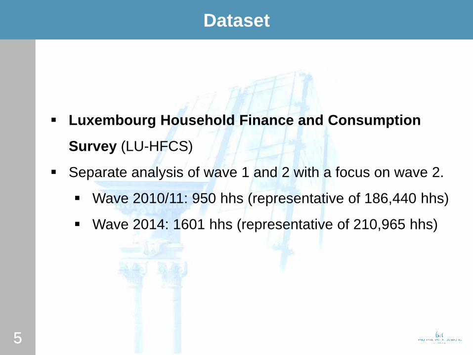
In order to calculate the debt burden indicators, this paper uses household micro data from the 1st and 2nd wave of the LU-HFCS. Both are representative samples of the population of households resident in Luxembourg. The 1st wave was conducted mostly in 2010 and included 950 households. The 2nd wave was conducted in 2014 and included 1601 households. Both waves were conducted by computer-assisted personal interviews (CAPI). Table 1 provides also the underlying

Household debt burden and financial vulnerability in Luxembourg 7
number of observations for the analysis. Four indicators are defined for the indebted population. The MDSI can only be calculated for households with mortgage debt and the outstanding LTV ratio (stock) is defined for HMR mortgage holders only.
Survey data are not free of drawbacks. In general, they suffer from a bias due to underreporting and missing responses, especially among the wealthiest households. In order to limit this bias, HFCS data is multiply imputed and the analyses included here account for uncertainty due to sampling and imputation methods. Unless indicated differently, the standard errors and confidence intervals reported below account for both sampling and imputation variability. They are based on 1000 replicate weights and 5 multiply imputed implicates of the dataset. This ensures a more accurate analysis of financial vulnerability for the full population of households resident in Luxembourg. References below to personal characteristics of a household (indicated by a *) always refer to those of the “financially knowledgeable person” (FKP). The FKP is the person within the household who was self-declared as the best informed about household finances and responded to survey questions on financial matters.
3 Results
We first describe the demographic and socio-economic characteristics of indebted households and provide an overview on the mean and median level of debt (subsection 3.1). Subsection 3.2 compares the debt burden indicators for 2010 and 2014 and subsection 3.3 identifies household characteristics most closely correlated with higher debt burden indicators in 2014. Subsection 3.4 compares the share of financially vulnerable households in 2010 and in 2014 and subsection 3.5 identifies household characteristics most closely correlated with financial vulnerability in 2014.
3.1 Indebted households
In 2014, 54.6% of all households were indebted. This is a 3.8 percentage point (ppt) decline compared to 2010. Girshina, Mathä, and Ziegelmeyer (2017; section 2.2) provide details on participation rates and mean/median debt across debt categories7 conditional on participation.
Figure 1 shows the population composition for all households and for indebted households according to various socio-demographic and economic variables for both 2010 and 2014. Indebted households are younger relative to the total population of households, have more household members, have more dependent children, and are less likely to be single and widowed. They are less likely to have low educational attainment and more likely to have high educational attainment. Indebted households are more likely to be (self-)employed, more likely to belong to the higher income quintiles, less likely to belong to the top or the bottom net
7 Mortgage debt comprises that on the HMR and that on other real estate property. Non-mortgage
debt includes overdraft debt, credit card debt, private and consumer loans.

8 Household debt burden and financial vulnerability in Luxembourg
wealth quintile, but more likely to belong to the second lowest net wealth quintile. More than half of indebted households have outstanding mortgage debt.
Population composition – all households and indebted households
Figure 1
Source: Own calculations based on the 1st and 2nd wave of the LU-HFCS; data are multiply imputed and weighted.
The share of households that were indebted declined from 2010 to 2014. However, among those households that were in debt, the mean level of total debt increased by 27% (the median level rose by 22%). The nominal mean value of debt reached € 178,400 in 2014 (the median level reached € 89,800). This increase was mainly driven by mortgage debt on the HMR and exceeded the increase in total real assets, whose mean value rose by only 4.3% (median value rose 7%). The different growth of debt and real assets corroborates the analysis in BCL (2016) and will influence the debt burden and vulnerability measures as discussed below.
0% 10% 20% 30% 40% 50% 60% 70% 80%
16-3435-4445-5455-64
65+
BelgiumFrance
GermanyItaly
LuxembourgOther countries
Portugal
Low (ISCED=0,1,2)Middle (ISCED=3,4)
High (ISCED=5,6)
EmployedSelf-Employed
UnemployedRetired
Other
FemaleMale
1 member2 members3 members4 members
5+ members
Owner-outright Owner-with mortgage
Renter or other
SingleCouple
DivorcedWidowed
1 child2 children
3+ childrenno children
Quintile 1Quintile 2Quintile 3Quintile 4Quintile 5
Quintile 1Quintile 2Quintile 3Quintile 4Quintile 5
Age
clas
ses*
Coun
try o
f birt
h*Ed
ucat
ion
leve
l*Em
ploy
men
t st
atus
*Ge
n-de
rHo
useh
old
size
Hous
ing
stat
usM
arita
l st
atus
*
Num
ber o
f de
pend
ent
child
ren
Tota
l gro
ss
inco
me
Tota
l net
wea
lth
2010: total population
2010: indebted households
0% 10% 20% 30% 40% 50% 60% 70% 80%
2014: total population
2014: indebted households

Household debt burden and financial vulnerability in Luxembourg 9
3.2 Debt burden indicators
Table 2 presents the median value of several debt burden indicators in the population of indebted households in Luxembourg. These ratios suggest that households that were indebted in 2014 carried a heavier debt burden than those that were indebted in 2010. The increase in debt exceeded the increase in the value of assets which could be pledged as collateral, as well as the increase in annual gross income. However, the p-values in the final column indicate that the difference between 2010 and 2014 was only statistically significant for the DI and outstanding LTV ratios (stock). The DSI ratio, instead, declined between 2010 and 2014, mainly driven by the lower cost of non-mortgage debt.
Median debt burden indicators
Table 2
Source: Own calculations based on the 1st and 2nd wave of the LU-HFCS; data are multiply imputed and weighted; variance estimation based on 1000 replicate weights. P-values indicate whether difference between 2010 and 2014 is significant: *** p<0.01, ** p<0.05, * p<0.1.
In part, these changes reflect macro-economic developments between the two waves of the survey. Weakness in the EA and abroad lead to a drop in inflation that prompted the Eurosystem to implement a series of unprecedented monetary policy measures (both conventional and unconventional). This lowered the cost of borrowing as well as the return on many financial investments. This context could explain why the increase in the median DA ratio was not statistically significant in Luxembourg. On the other hand, the statistically significant increase in the DI ratio may reflect the fact that around 70% of indebted households are reported as “employed” (see Figure 1), and wages progressed little given low inflation during those years (mean household gross income increased by only 4% between 2010 and 2014; the median was unchanged). Finally, the accommodating monetary policy stance contributes to lower the cost of debt service.
Debt burden indicators Year Median Std. err. p-value2010 18.2% 2.1% 14.6% 21.7%2014 22.2% 2.1% 18.7% 25.6%2010 86.9% 11.2% 68.4% 105.4%2014 114.1% 10.6% 96.7% 131.5%2010 15.7% 0.9% 14.3% 17.2%2014 14.8% 0.6% 13.8% 15.8%2010 16.3% 0.7% 15.2% 17.3%2014 17.6% 0.7% 16.4% 18.7%2010 27.5% 2.6% 23.2% 31.7%2014 34.6% 2.8% 30.1% 39.2%
2010 12.2% 2.2% 8.6% 15.9%2014 11.5% 1.7% 8.8% 14.2%
36.7%Debt service-to-income ratio
Mortgage debt service-to-income
Outstanding loan-to-value ratio of main residence (stock)
Net liquid assets to income 79.0%
5.6% *
17.3%
[90% conf. interval]
16.1%Debt-to-asset ratio
Debt-to-income ratio 8.9% *
10 Household debt burden and financial vulnerability in Luxembourg
3.3 Linking debt burden and household characteristics
We use a median regression8 (see Christelis et al. 2013; Bauer et al., 2011) to quantify the correlation between the debt burden indicators defined above and the household characteristics shown in Table 3.9 We run the median regressions only for 2014 as we are interested in identifying groups of households with higher debt burdens using the most recent data (estimated coefficients are shown in Table 3). A statistically significant effect on the median identifies correlation not necessarily causation, so the results should be interpreted as descriptive analysis. For some indicators, income or wealth appears on both sides of the regression (as a ratio for the dependent variable and a set of dummy variables for the independent variables), so we acknowledge that there is a potential simultaneity bias, although this may be limited given the different nonlinear transformations used. Despite this drawback, the regression approach provides the important advantage that we can control for other explanatory variables when testing for a significant correlation.
The benchmark or reference group is defined for each explanatory variable separately: it is a household with a male FKP, between 16 and 34 years old, born in Luxembourg, low educated, married, and employed. Referring to the household characteristics the reference group is also defined for each explanatory variable separately: single person household, no dependent children, renting the HMR, belonging to the highest quintiles of gross income and net wealth. Given that our independent variables are all binary, the estimated coefficients presented in Table 3 indicate the difference with respect to the median of the reference group. The estimated coefficient on the intercept term represents the median of the reference group. Coefficient estimates reported in Table 3 demonstrate that some household characteristics are significantly related to the debt burden indicators. These characteristics include net wealth quintiles, age classes, and (to a lesser extent) gross income quintiles. As will be explained below, the pattern of the estimated coefficients is consistent with theoretical models of the life-cycle (Modigliani and Brumberg, 1954; Friedman, 1957). First, net wealth correlates negatively with most debt burden indicators (except the DSI ratio). This was expected, particularly for the DA ratio and the outstanding LTV ratio (stock), as higher assets (or lower debts) increase net wealth while reducing these ratios. Less wealthy households have less net liquid assets relative to their gross income, as confirmed by the larger (negative) coefficient for higher net wealth quintiles in column 6 (Net liquid assets to income ratio).10 For instance, a household in the middle net wealth quintile has a median ratio of net liquid assets to gross income which is 64ppt smaller than in the highest net wealth quintile. Surprisingly, differences in the median NLAI ratio across gross income quintiles are not statistically significant.
8 Median regression, also known as least-absolute-deviations regression, is a quantile regression
at the median. While quantile regression minimizes a sum of absolute errors with asymmetric penalties for over- and underprediction, the median regression uses symmetric penalties and therefore provides the optimal prediction at the conditional median.
9 We use a bootstrap procedure for complex survey data using the bs4rw command in Stata. It is based on 1000 replicate weights to ensure that our estimates are representative of the population (Kolenikov, 2010).
10 Net wealth quintiles are almost the only explanatory variables significantly correlated with the median NLAI.

Household debt burden and financial vulnerability in Luxembourg 11
Median regression – Debt burden indicators on household characteristics – 2014
Table 3
Source: Own calculations based on the 2nd wave of the LU-HFCS; data are multiply imputed and weighted; variance estimation based on 1000 replicate weights. The reference group is defined for each explanatory variable separately: it is a household with a male FKP, between 16 and 34 years old, born in Luxembourg, low educated, married, and employed. Referring to the household characteristics the reference group is also defined for each explanatory variable separately: single person household, no dependent children, renting the HMR, belonging to the highest quintiles of gross income and net wealth. Dummies related to household size and marital status are not shown as they are not statistically significant. Significant results are highlighted in grey.
(1) (2) (3) (4) (5) (6)
VARIABLESDebt-to-asset
ratioDebt-to-income
ratioDebt service-to-
income ratio
Mortgage debt service-to-
income ratio
Outstanding loan-to-value ratio of
HMR (stock)
Net l iquid assets as a fraction of
annual gross income
Female 0.009 0.097 0.013 0.016 0.005 0.058(0.025) (0.150) (0.012) (0.014) (0.027) (0.049)
Age class 35-44 -0.053 -0.002 0.020 0.013 -0.091* 0.013(0.047) (0.259) (0.016) (0.021) (0.049) (0.065)
Age class 45-54 -0.144*** -0.594*** -0.009 -0.005 -0.231*** -0.010(0.052) (0.229) (0.018) (0.026) (0.059) (0.086)
Age class 55-64 -0.154*** -0.835*** 0.003 -0.018 -0.265*** 0.076(0.052) (0.275) (0.021) (0.030) (0.064) (0.117)
Age class 65+ -0.117* -0.753** 0.020 0.023 -0.193 0.161(0.063) (0.340) (0.036) (0.046) (0.160) (0.199)
Country of birth: PT 0.034 0.071 -0.042* -0.059** 0.053 0.081(0.048) (0.282) (0.024) (0.027) (0.056) (0.068)
Country of birth: FR -0.035 -0.300 0.011 -0.010 -0.024 -0.023(0.038) (0.231) (0.020) (0.027) (0.063) (0.089)
Country of birth: BE -0.027 -0.307 -0.023 -0.041 0.060 0.126(0.046) (0.260) (0.027) (0.032) (0.074) (0.157)
Country of birth: IT 0.080 0.088 -0.031 0.012 0.116** 0.061(0.310) (0.338) (0.032) (0.037) (0.059) (0.123)
Country of birth: DE 0.061 0.043 0.024 0.002 0.051 0.153(0.055) (0.679) (0.032) (0.029) (0.064) (0.304)
Country of birth: Other -0.056* -0.560*** -0.037** -0.049*** -0.012 0.007(0.030) (0.203) (0.015) (0.018) (0.038) (0.084)
1 child 0.078** 0.275 0.021 0.030 0.063 -0.105(0.035) (0.247) (0.020) (0.023) (0.053) (0.083)
2 children 0.051 0.108 0.012 0.017 0.027 -0.132(0.039) (0.287) (0.024) (0.030) (0.064) (0.103)
3+ children 0.082 0.144 0.049 0.008 0.068 -0.179(0.063) (0.487) (0.038) (0.061) (0.110) (0.166)
Education: ISCED=3,4 0.008 0.028 -0.025 -0.025 0.031 0.102(0.028) (0.193) (0.020) (0.024) (0.049) (0.062)
Education: ISCED=5,6 0.043 0.319 -0.023 -0.005 0.091* 0.179*(0.034) (0.244) (0.022) (0.027) (0.053) (0.092)
Self-employed 0.034 0.227 -0.027 0.022 0.090 -0.073(0.040) (0.330) (0.032) (0.044) (0.064) (0.108)
Unemployed -0.179 -0.481 -0.084* -0.059 -0.130 0.105(0.115) (0.391) (0.047) (0.055) (0.164) (0.177)
Retired -0.011 0.062 -0.061*** -0.054* 0.014 -0.096(0.029) (0.219) (0.022) (0.028) (0.052) (0.123)
Other employment status -0.005 0.085 -0.039* -0.022 -0.001 -0.120(0.053) (0.258) (0.022) (0.052) (0.141) (0.131)
Owner-outright 0.084* 0.916*** 0.010 -0.158(0.046) (0.328) (0.021) (0.133)
Owner with mortgage 0.174*** 2.246*** 0.111*** -0.065(0.041) (0.300) (0.018) (0.081)
Gross income quintile 1 -0.113** 0.573 0.153*** 0.208* -0.173** 0.041(0.057) (0.355) (0.049) (0.117) (0.084) (0.115)
Gross income quintile 2 -0.044 0.286 0.080*** 0.142*** -0.067 0.003(0.040) (0.308) (0.019) (0.034) (0.059) (0.110)
Gross income quintile 3 -0.046 0.318 0.063*** 0.101*** -0.063 0.035(0.029) (0.210) (0.015) (0.022) (0.046) (0.084)
Gross income quintile 4 -0.027 0.277 0.022 0.035** -0.038 -0.031(0.025) (0.198) (0.014) (0.017) (0.036) (0.069)
Net wealth quintile 1 0.852*** 0.695* -0.012 0.206* 0.974*** -1.023***(0.112) (0.402) (0.030) (0.120) (0.205) (0.191)
Net wealth quintile 2 0.361*** 1.088*** 0.022 0.019 0.412*** -0.751***(0.035) (0.305) (0.019) (0.031) (0.049) (0.163)
Net wealth quintile 3 0.103*** -0.004 0.001 0.009 0.163*** -0.642***(0.036) (0.242) (0.017) (0.021) (0.040) (0.148)
Net wealth quintile 4 0.039* -0.150 -0.009 0.007 0.068* -0.564***(0.022) (0.194) (0.016) (0.017) (0.036) (0.162)
Constant 0.085 -0.122 0.056 0.098* 0.244** 0.827***(0.075) (0.562) (0.039) (0.051) (0.098) (0.214)
Observations 952 952 952 664 547 952Standard errors in parentheses, *** p<0.01, ** p<0.05, * p<0.1

12 Household debt burden and financial vulnerability in Luxembourg
Second, columns 1, 2 and 5 suggest that debt is lower among households where the FKP is older. The outstanding LTV ratio (stock) declines with age, confirming that households purchase their main residence at early stages of their active life.
As expected, the median DSI and MDSI ratios (columns 3 and 4) gradually decline with gross income. However, the first quintile of gross income is associated with a significantly lower DA ratio and a lower outstanding LTV ratio (stock). These results indicate that low income households are also those with the lowest median leverage.
3.4 Vulnerable households
3.4.1 Single indicator approach
For each debt burden indicator, Table 4 reports the share of the population of indebted households that are identified as financially vulnerable. Comparing the wave in 2010 to the one in 2014, these results do not signal a substantial change in financial vulnerability. The only statistically significant increase (at the 5% significance level) is for the share of households with a DI ratio higher or equal than 3. The increases in the share of households with DSI ≥ 40% and those with MDSI ≥ 40% are not statistically significant. Finally, the share of households with outstanding LTV ≥ 75% is lower than in 2010 (not statistically significant), possibly reflecting regulatory changes introduced between the two waves. These changes in the share of vulnerable households tend to be consistent with changes in median debt burden indicators (described in section 3.2).
Share of vulnerable households: single indicator approach
Table 4
Source: Own calculations based on the 1st and 2nd wave of the LU-HFCS; data are multiply imputed and weighted; variance estimation based on 1000 replicate weights. P-values indicate whether difference between 2010 and 2014 is significant: *** p<0.01, ** p<0.05, * p<0.1.
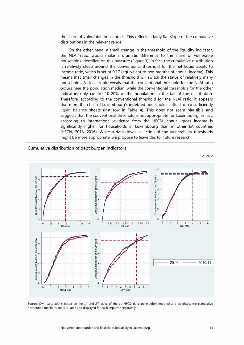
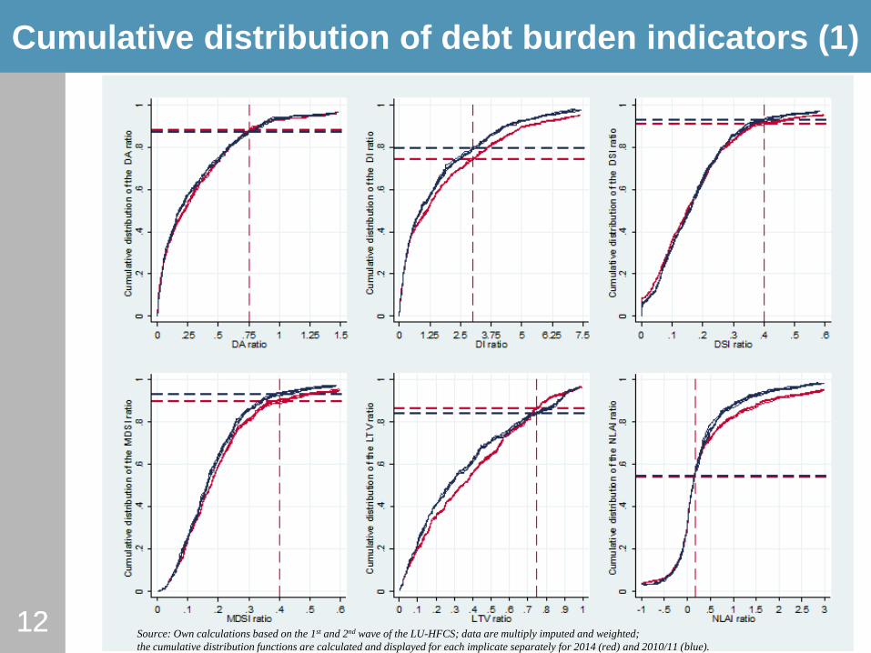
The vulnerability thresholds we employ are conventional in the literature, but they remain somewhat arbitrary. In order to assess the robustness of the result (share of vulnerable households) to alternative values of the threshold, Figure 2 depicts the cumulative distributions for each debt burden indicator in 2010 (blue lines) and in 2014 (red lines). The dashed horizontal lines represent the conventional thresholds reported in Table 1 and applied in Table 4. Moderate changes in the threshold around their conventional levels would not generally produce significant changes in
Vulnerability measures Year Mean Std. err. p-value2010 12.8% 1.6% 10.2% 15.5%2014 12.0% 1.4% 9.7% 14.3%2010 20.6% 1.9% 17.5% 23.7%2014 25.8% 1.8% 22.8% 28.8%2010 7.0% 1.3% 4.9% 9.2%2014 8.9% 1.3% 6.8% 11.0%2010 6.8% 1.6% 4.1% 9.5%2014 10.3% 1.7% 7.4% 13.1%2010 15.9% 2.3% 12.0% 19.8%2014 13.4% 1.9% 10.3% 16.4%
2010 55.5% 2.5% 51.4% 59.7%2014 55.7% 1.9% 52.6% 58.9%
[90% conf. interval]
Debt-to-income ratio ≥ 3
Debt service-to-income ratio ≥ 40%
Mortgage debt service-to-income ratio ≥ 40%
Outstanding loan-to-value ratio of main residence (stock) ≥ 75%
94.6%Net liquid assets < 2 months income
70.0%
4.7% **
31.4%
10.7%
40.7%
Debt-to-asset ratio ≥ 75%
Household debt burden and financial vulnerability in Luxembourg 13
the share of vulnerable households. This reflects a fairly flat slope of the cumulative distributions in the relevant range.
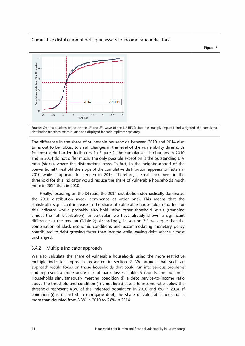
On the other hand, a small change in the threshold of the liquidity indicator, the NLAI ratio, would make a dramatic difference to the share of vulnerable households identified on this measure (Figure 3). In fact, the cumulative distribution is relatively steep around the conventional threshold for the net liquid assets to income ratio, which is set at 0.17 (equivalent to two months of annual income). This means that small changes in the threshold will switch the status of relatively many households. A closer look reveals that the conventional threshold for the NLAI ratio occurs near the population median, while the conventional thresholds for the other indicators only cut off 10-20% of the population in the tail of the distribution. Therefore, according to the conventional threshold for the NLAI ratio, it appears that more than half of Luxembourg’s indebted households suffer from insufficiently liquid balance sheets (last row in Table 4). This does not seem plausible and suggests that the conventional threshold is not appropriate for Luxembourg. In fact, according to international evidence from the HFCN, annual gross income is significantly higher for households in Luxembourg than in other EA countries (HFCN, 2013, 2016). While a data-driven selection of the vulnerability thresholds might be more appropriate, we propose to leave this for future research.
Cumulative distribution of debt burden indicators
Figure 2
Source: Own calculations based on the 1st and 2nd wave of the LU-HFCS; data are multiply imputed and weighted; the cumulative distribution functions are calculated and displayed for each implicate separately.
0.2
.4.6
.81
Cum
ulat
ive
dist
ribut
ion
of th
e D
A ra
tio
0 .25 .5 .75 1 1.25 1.5DA ratio
0.2
.4.6
.81
Cum
ulat
ive
dist
ribut
ion
of th
e D
I rat
io
0 1.25 2.5 3.75 5 6.25 7.5DI ratio
0.2
.4.6
.81
Cum
ulat
ive
dist
ribut
ion
of th
e D
SI ra
tio
0 .1 .2 .3 .4 .5 .6DSI ratio
0.2
.4.6
.81
Cum
ulat
ive
dist
ribut
ion
of th
e M
DSI
ratio
0 .1 .2 .3 .4 .5 .6MDSI ratio
0.2
.4.6
.81
Cum
ulat
ive
dist
ribut
ion
of th
e LT
V ra
tio
0 .1 .2 .3 .4 .5 .6 .7 .8 .9 1LTV ratio
14 Household debt burden and financial vulnerability in Luxembourg
Cumulative distribution of net liquid assets to income ratio indicators
Figure 3
Source: Own calculations based on the 1st and 2nd wave of the LU-HFCS; data are multiply imputed and weighted; the cumulative distribution functions are calculated and displayed for each implicate separately.
The difference in the share of vulnerable households between 2010 and 2014 also turns out to be robust to small changes in the level of the vulnerability thresholds for most debt burden indicators. In Figure 2, the cumulative distributions in 2010 and in 2014 do not differ much. The only possible exception is the outstanding LTV ratio (stock), where the distributions cross. In fact, in the neighbourhood of the conventional threshold the slope of the cumulative distribution appears to flatten in 2010 while it appears to steepen in 2014. Therefore, a small increment in the threshold for this indicator would reduce the share of vulnerable households much more in 2014 than in 2010.
Finally, focussing on the DI ratio, the 2014 distribution stochastically dominates the 2010 distribution (weak dominance at order one). This means that the statistically significant increase in the share of vulnerable households reported for this indicator would probably also hold using other threshold levels (spanning almost the full distribution). In particular, we have already shown a significant difference at the median (Table 2). Accordingly, in section 3.2 we argue that the combination of slack economic conditions and accommodating monetary policy contributed to debt growing faster than income while leaving debt service almost unchanged.
3.4.2 Multiple indicator approach
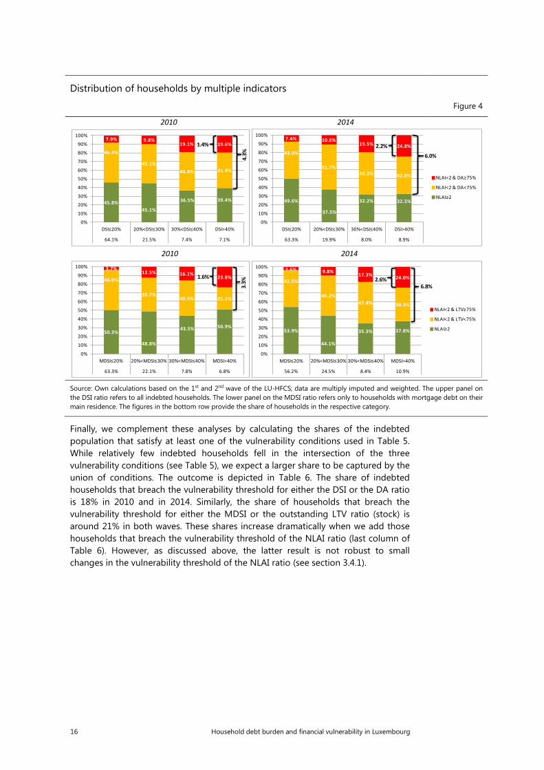
We also calculate the share of vulnerable households using the more restrictive multiple indicator approach presented in section 2. We argued that such an approach would focus on those households that could run into serious problems and represent a more acute risk of bank losses. Table 5 reports the outcome. Households simultaneously meeting condition (i) a debt service-to-income ratio above the threshold and condition (ii) a net liquid assets to income ratio below the threshold represent 4.3% of the indebted population in 2010 and 6% in 2014. If condition (i) is restricted to mortgage debt, the share of vulnerable households more than doubled from 3.3% in 2010 to 6.8% in 2014.
0.2
.4.6
.81
Cum
ulat
ive
dist
ribut
ion
of th
e N
LAI r
atio
-1 -.5 0 .5 1 1.5 2 2.5 3NLAI ratio

Household debt burden and financial vulnerability in Luxembourg 15
Share of vulnerable households across waves: multiple indicator approach
Table 5
Source: Own calculations based on the 1st and 2nd wave of the LU-HFCS; data are multiply imputed and weighted. The rows on the DSI ratio refer to all indebted households. The rows on the MDSI ratio refer only to households with mortgage debt on their main residence.
Bank losses will only be important if these vulnerable households are also highly leveraged. When we add condition (iiia), a DA ratio breaching the threshold, there remain 1.4% of indebted households in 2010 and 2.2% in 2014 (the change between years is not statistically significant). If instead we add condition (iiib), the outstanding LTV ratio (stock) on the HMR breaching the threshold, there remain 1.6% of indebted households in 2010 and 2.6% in 2014 (the change between years is not statistically significant). The aggregate value of banks’ exposure of default can be approximated by summing up the debt holdings of these population shares. In future research, we plan to calculate loss given default, exposure at default and probabilities of default at the individual household level in a stress test of household balance sheets.
While Table 5 focuses on households with a debt service-to-income ratio above the 40% threshold, Figure 4 provides more detailed information on the whole distribution of indebted households, including those with DSI ratios below the threshold. The upper panel refers to the population of all indebted households, while the bottom one focuses only on households with mortgage debt on their main residence. The bar on the far right in each panel provides the same information as in Table 5.
Most households have moderate DSI ratios below 20% or 30% (first two columns on the left account for 83.2% of indebted households in 2014). Comparing household groups according to their DSI ratios (the different bars) reveals heterogeneous distributions of the NLAI ratio. In 2014, the share of households with net liquid assets above 2 months income (green segment) decreases from around 50% for indebted households with a DSI below 20% (first bar) to around 32% for households with a DSI above 30% (last two bars). In addition, the share of households that combine an insufficient NLAI ratio with an excessive DA ratio (red segment) increases from 7% for households with a DSI below 20% (first bar) to 25% for households with a DSI of more than 40% (last bar). Thus, households with high DSI ratios tend to have proportionally less favourable NLAI and DA ratios. The pattern is generally confirmed if we focus on debt service-to-income ratio from mortgage on the main residence only (lower panel).
(i) (ii) (iiia) (iiib)
YearDSI ratio ≥ 40% or MDSI ratio ≥ 40%
Net liquid assets < 2 months
incomeDA ratio ≥ 75%
Outstanding LTV ratio of HMR (stock)
≥ 75%
2010 7.1 4.3 1.4 -2014 8.9 6.0 2.2 -2010 6.8 3.3 - 1.62014 10.9 6.8 - 2.6
Additional conditions
DSI ratio ≥ 40%
MDSI ratio ≥ 40%
16 Household debt burden and financial vulnerability in Luxembourg
Distribution of households by multiple indicators
Figure 4
2010 2014
2010 2014
Source: Own calculations based on the 1st and 2nd wave of the LU-HFCS; data are multiply imputed and weighted. The upper panel on the DSI ratio refers to all indebted households. The lower panel on the MDSI ratio refers only to households with mortgage debt on their main residence. The figures in the bottom row provide the share of households in the respective category.
Finally, we complement these analyses by calculating the shares of the indebted population that satisfy at least one of the vulnerability conditions used in Table 5. While relatively few indebted households fell in the intersection of the three vulnerability conditions (see Table 5), we expect a larger share to be captured by the union of conditions. The outcome is depicted in Table 6. The share of indebted households that breach the vulnerability threshold for either the DSI or the DA ratio is 18% in 2010 and in 2014. Similarly, the share of households that breach the vulnerability threshold for either the MDSI or the outstanding LTV ratio (stock) is around 21% in both waves. These shares increase dramatically when we add those households that breach the vulnerability threshold of the NLAI ratio (last column of Table 6). However, as discussed above, the latter result is not robust to small changes in the vulnerability threshold of the NLAI ratio (see section 3.4.1).
45.8%45.1%
36.5% 39.4%
46.4%
45.1%44.4% 41.0%
7.9% 9.8%19.1% 19.6%
0%
10%
20%
30%
40%
50%
60%
70%
80%
90%
100%
DSI≤20% 20%<DSI≤30% 30%<DSI≤40% DSI>40%
64.1% 21.5% 7.4% 7.1%4.
3%
1.4%
49.6%
37.5%
32.2% 32.5%
43.0%
51.7%48.3% 42.8%
7.4% 10.8%19.5% 24.8%
0%
10%
20%
30%
40%
50%
60%
70%
80%
90%
100%
DSI≤20% 20%<DSI≤30% 30%<DSI≤40% DSI>40%
63.3% 19.9% 8.0% 8.9%
NLAI<2 & DA≥75%
NLAI<2 & DA<75%
NLAI≥2
6.0%
2.2%
50.3%
48.8%
43.5% 50.9%
46.0%
38.7%40.5% 25.3%
3.7%12.5% 16.1%
23.8%
0%
10%
20%
30%
40%
50%
60%
70%
80%
90%
100%
MDSI≤20% 20%<MDSI≤30% 30%<MDSI≤40% MDSI>40%
63.3% 22.1% 7.8% 6.8%
3.3%
1.6%
53.9%
44.1%
35.3% 37.8%
42.5%
46.2%47.4% 38.3%
3.6% 9.8% 17.3% 24.0%
0%
10%
20%
30%
40%
50%
60%
70%
80%
90%
100%
MDSI≤20% 20%<MDSI≤30% 30%<MDSI≤40% MDSI>40%
56.2% 24.5% 8.4% 10.9%
NLAI<2 & LTV≥75%
NLAI<2 & LTV<75%
NLAI≥2
6.8%2.6%

Household debt burden and financial vulnerability in Luxembourg 17
Share of households classified as vulnerable by at least one indicator
Table 6
Source: Own calculations based on the 1st and 2nd wave of the LU-HFCS; data are multiply imputed and weighted. The rows on the DSI ratio refer to all indebted households. The rows on the MDSI ratio refer only to households with mortgage debt on their main residence.
3.5 Linking vulnerability and household characteristics
We use a probit model to estimate the probability that a given household is classified as vulnerable (using the conventional thresholds and the standard single indicator approach). This adds to the median regression on the debt burden indicators as the probit model helps identifying the characteristics of vulnerable households which are by definition in the tail of the corresponding distribution (the conventional vulnerability thresholds are, for 5 out of 6 measures, at the right tail of the distribution, Figure 2 and Figure 3). As one can see below, the relevant characteristics differ in the two exercises.
The dependent variable is unity if the household is identified as vulnerable on a given measure and zero otherwise. Thus, the model can be written as follows:
( ) ( ) ( ) |0Pr|1Pr * xxVxV ii Φ=>== (1)
0*
iiXi XV εββ ++= (2)
Household i’s probability of being classified as vulnerable is expressed as a function of several determinants x, which influence a latent variable *Vi . We use the
same explanatory variables as for the median regression on debt burden indicators (Table 3). Again, we aim to identify household characteristics which are correlated with financial vulnerability while controlling for other household characteristics. Marginal effects are calculated at the observation level and then averaged. Potential simultaneity bias may also arise in this setting. Table 7 reports the estimated average marginal effects. These are strong for net wealth, gross income and the age of the FKP in the household. Including four net wealth quintiles allows the DA ≥ 75% regression in column 1 to perfectly identify households in our sample. This is why only the first net wealth quintile is included in column 1. In column 5, the marginal effect on the probability that LTV ≥ 75% is highest for households in the first net wealth quintile and the marginal effects tend to decrease with higher wealth. For instance, the probability that a household in the lowest net wealth quintile is vulnerable is 54% higher compared to a household in the reference (highest) quintile. In column 6, low net liquid assets relative to gross income are more likely for low wealth households. Marginal effects decline steadily with higher
(iia) (iib) (iii)
YearDA ratio
≥ 75%
Outstanding LTV ratio of HMR (stock)
≥ 75%
Net liquid assets < 2 months income
2010 18.0 - 60.72014 18.0 - 59.32010 - 21.1 73.92014 - 21.2 73.4
Additional conditions
DSI ratio ≥ 40%
MDSI ratio ≥ 40%

18 Household debt burden and financial vulnerability in Luxembourg
wealth. In column 4, the probability that the MDSI ratio exceeds 40% is significantly higher for households in the lowest net wealth quintile compared to those in the reference (highest) quintile. The average marginal effects in this column are negative for quintiles 2 and 3. This means that households belonging to these middle quintiles are less likely to be classified as vulnerable on this criterion compared to those in the reference (highest) net wealth quintile.
As expected, gross income tends to play a significant role in columns 3 and 4 (probability that total DSI or MDSI exceeds 40%). According to these indicators, the probability of being identified as vulnerable is lowest for the top gross income quintile and increases steadily as one approaches the lower end of the income distribution.
If the indicator is based on the stock of debt (columns 1, 2 and 5), the probability that the household will be classified as vulnerable decreases with the age of the FKP. This is consistent with the life cycle pattern of indebtedness, which suggests that high DI ratios are in line with models of optimal portfolio choice over the life-cycle.
Some results in Table 7 may appear puzzling at first sight, such as those concerning ownership status, education level and occupation. The positive and highly significant coefficient for outright owners compared to renters might be surprising in columns 2, 3 and 6. We also ran the regressions omitting net wealth quintiles from the set of explanatory variables (results not shown to save space). In this case, owners (with or without a mortgage) were less likely to be identified as vulnerable in column 6. This suggests a high correlation between net wealth and housing status that may be biasing the coefficient on the latter variable.
Similarly, in columns 2 and 4 households where the FKP is highly educated tend to be more vulnerable. This may be related to a higher potential income growth. Likewise, in columns 2-4 households where the FKP is self-employed are more likely to be vulnerable, while in column 1 those where the FKP is unemployed are less likely to be vulnerable. The latter result might be explained by credit constraints facing the unemployed.
We conclude that highly leveraged households (columns 1, 2 and 5) and household with a high debt servicing burden (columns 3 and 4) tend, on the one hand, to be part of the less vulnerable socio-economic groups of the population (in terms of education, employment and HMR ownership status) but, on the other hand, also to be part of more vulnerable groups (low income and wealth), which is at least partly opposite to the findings for the median regression reported in Table 3.

Household debt burden and financial vulnerability in Luxembourg 19
Probit regression - Probability of financial vulnerability on household characteristics - 2014 Table 7
Source: Own calculations based on the 2nd wave of the LU-HFCS; data are multiply imputed and weighted; variance estimation based on final weights. The reference group is defined for each explanatory variable separately: it is a household with a male FKP, between 16 and 34 years old, born in Luxembourg, low educated, married, and employed. Referring to the household characteristics the reference group is also defined for each explanatory variable separately: single person household, no dependent children, renting the HMR, belonging to the highest quintiles of gross income and net wealth. Marginal effects are calculated at the observation level and then averaged. Dummies related to the marital status are not shown as they are not statistically significant. Significant results are highlighted in grey.
(1) (2) (3) (4) (5) (6)
VARIABLESDebt-to-asset
ratio ≥ 75%Debt-to-income
ratio ≥ 3
Debt service-to-income ratio
≥ 40 %
Mortgage debt service-to-
income ratio ≥ 40 %
Outstanding loan-to-value ratio (stock) ≥ 75 %
Net l iquid assets < 2 months gross
income
Female 0.016 0.006 0.004 -0.025 0.040 -0.049(0.020) (0.029) (0.022) (0.025) (0.028) (0.039)
Age class 35-44 -0.059** -0.026 0.013 0.045 -0.080** 0.033(0.026) (0.042) (0.028) (0.034) (0.035) (0.061)
Age class 45-54 -0.104*** -0.173*** -0.033 0.002 -0.110** 0.086(0.031) (0.047) (0.036) (0.043) (0.047) (0.064)
Age class 55-64 -0.159*** -0.207*** -0.009 -0.000 -0.176*** -0.046(0.049) (0.074) (0.055) (0.063) (0.065) (0.073)
Age class 65+ 0.008 -0.081 -0.035 -0.049 † -0.094(0.059) (0.101) (0.087) (0.088) (0.115)
Country of birth: PT -0.001 -0.036 -0.036 -0.067 0.075* -0.075(0.032) (0.052) (0.035) (0.050) (0.040) (0.066)
Country of birth: FR -0.029 -0.067 -0.116** -0.103 0.054 0.026(0.034) (0.054) (0.045) (0.064) (0.051) (0.073)
Country of birth: BE 0.001 -0.120 -0.201*** -0.146*** 0.064 -0.168*(0.037) (0.075) (0.055) (0.054) (0.062) (0.099)
Country of birth: IT 0.055 -0.020 -0.101** -0.082* 0.064 -0.043(0.044) (0.084) (0.048) (0.049) (0.068) (0.093)
Country of birth: DE -0.108** 0.064 0.079 0.065 -0.275*** -0.045(0.045) (0.101) (0.060) (0.051) (0.090) (0.114)
Country of birth: Other -0.074** -0.177*** -0.099*** -0.076* -0.096* -0.012(0.034) (0.049) (0.037) (0.040) (0.058) (0.057)
Household size: 2 0.025 -0.022 0.072** 0.101** 0.091* 0.109(0.036) (0.055) (0.035) (0.044) (0.053) (0.070)
Household size: 3 -0.012 -0.092 0.042 0.080 0.017 0.228**(0.056) (0.072) (0.052) (0.065) (0.077) (0.096)
Household size: 4 0.040 -0.012 0.068 0.115* 0.020 0.181*(0.054) (0.079) (0.061) (0.067) (0.068) (0.102)
Household size: 5 -0.116 -0.070 0.155** 0.245*** -0.504 0.203(0.226) (0.105) (0.069) (0.072) (0.312) (0.164)
1 child 0.004 0.117** -0.003 -0.027 -0.037 -0.009(0.048) (0.054) (0.041) (0.047) (0.055) (0.077)
2 children -0.011 0.025 -0.019 -0.052 -0.001 -0.028(0.050) (0.062) (0.052) (0.060) (0.064) (0.079)
3+ children 0.191 0.100 -0.041 -0.078 0.631** 0.044(0.217) (0.098) (0.061) (0.067) (0.305) (0.154)
Single -0.066** -0.013 -0.007 -0.000 -0.014 0.078(0.030) (0.042) (0.032) (0.038) (0.035) (0.051)
Divorced 0.018 0.059 0.022 0.023 0.017 0.034(0.035) (0.048) (0.032) (0.038) (0.049) (0.067)
Widowed 0.077 -0.127 -0.011 † † -0.046(0.048) (0.140) (0.073) (0.106)
Education: ISCED=3,4 -0.000 0.024 0.008 0.051 0.056 -0.146***(0.027) (0.046) (0.026) (0.031) (0.040) (0.056)
Education: ISCED=5,6 0.005 0.088* 0.029 0.063* 0.028 -0.221***(0.033) (0.054) (0.031) (0.035) (0.057) (0.062)
Self-employed -0.055 0.105** 0.081** 0.102*** -0.023 0.083(0.038) (0.050) (0.033) (0.035) (0.058) (0.075)
Unemployed -0.133** -0.219 † † † -0.002(0.066) (0.133) (0.118)
Retired -0.148*** 0.015 0.001 0.028 † 0.043(0.049) (0.101) (0.074) (0.070) (0.083)
Other employment status 0.012 0.004 0.018 0.060 0.018 0.036(0.037) (0.068) (0.043) (0.046) (0.050) (0.087)
Owner-outright -0.089 0.160** 0.086* 0.162**(0.062) (0.070) (0.052) (0.079)
Owner with mortgage 0.071** 0.358*** 0.146*** 0.076(0.036) (0.053) (0.045) (0.067)
Gross income quintile 1 0.080* 0.209*** 0.278*** 0.347*** 0.003 -0.007(0.045) (0.079) (0.051) (0.059) (0.072) (0.096)
Gross income quintile 2 0.060 0.259*** 0.170*** 0.235*** 0.007 0.006(0.040) (0.059) (0.041) (0.048) (0.075) (0.071)
Gross income quintile 3 0.092*** 0.167*** 0.086** 0.111** -0.019 0.023(0.031) (0.050) (0.043) (0.047) (0.046) (0.059)
Gross income quintile 4 0.029 0.132*** 0.066* 0.081** -0.034 0.012(0.030) (0.045) (0.037) (0.041) (0.043) (0.049)
Net wealth quintile 1 0.257*** 0.089 0.045 0.156*** 0.543*** 0.726***(0.030) (0.079) (0.054) (0.053) (0.078) (0.094)
Net wealth quintile 2 † 0.138*** -0.040 -0.076* 0.160*** 0.384***(0.052) (0.038) (0.043) (0.049) (0.074)
Net wealth quintile 3 † -0.005 -0.084** -0.156*** 0.038 0.248***(0.051) (0.037) (0.042) (0.050) (0.059)
Net wealth quintile 4 † 0.001 -0.054 -0.041 0.073 0.171***(0.051) (0.035) (0.039) (0.061) (0.063)
Observations 952 952 952 664 547 952Standard errors in parentheses; *** p<0.01, ** p<0.05, * p<0.1; † variable omitted to avoid perfect coll inearity.
20 Household debt burden and financial vulnerability in Luxembourg
4 Conclusion
This paper investigates household financial vulnerability in Luxembourg using balance sheet information from the 1st (2010) and 2nd (2014) wave of the Luxembourg Household Finance and Consumption Survey. To account for different dimensions of household vulnerability, we calculate several indicators for each household in a representative sample.
The evidence we provide does not lead to one overarching key message but draws a mixed picture on the changes of household indebtedness and financial vulnerability in Luxembourg across the two currently available waves (the third wave is planned to be conducted at the end of 2017/ beginning of 2018). Indebted households in 2014 carried a heavier burden than indebted households in 2010, mainly because of mortgage loans on the main residence. However, increases in the median ratios between 2010 and 2014 are only statistically significant for the debt-to-income ratio and the outstanding loan-to-value ratio (stock). The median debt service-to-income ratio declined, although mostly due to lower costs of non-mortgage debt.
First we analyse the distribution of median debt burden indicators across household characteristics. The median regression estimates indicate that low income households are also those with the lowest median leverage. Thus, debt appears to be concentrated on the less vulnerable households.
Then we identify financially vulnerable households as those where debt burden indicators exceed conventional thresholds. On several measures, financial vulnerability of indebted households appears to have increased between 2010 and 2014. However, only the debt-to-income ratio suggests a statistically significant increase in the share of vulnerable households. On the one hand, disadvantaged socio-economic groups (in terms of education, employment status and HMR ownership status) are less often financially vulnerable. On the other hand, low income and wealth increases the likelihood of households’ vulnerability.
In addition to the standard single indicator approach, we also combine the information derived from several indicators. The multiple indicator approach shows a larger increase (in relative terms) than the single indicator approach but the increase is still not statistically significant. The share of financially vulnerable households is 2.2% of the indebted population and 2.6% of the population with mortgages on their main residence in 2014.
Finally, we conclude with some suggestions for further research. First, our assessment of household financial vulnerability depends on the thresholds chosen for the different indicators. These are set at conventional levels that remain somewhat arbitrary. In future research one could develop a data driven selection of these thresholds when measuring household financial vulnerability. Second, the impact of a rise in household financial vulnerability on bank balance sheets also depends on other negative shocks facing the sector. Therefore, we plan to implement alternative severe but plausible macroeconomic scenarios in a stress test of individual Luxembourg households.
Household debt burden and financial vulnerability in Luxembourg 21
5 References
Albacete, N., and P. Lindner (2013): Household Vulnerability in Austria – A Microeconomic Analysis Based on the Household Finance and Consumption Survey. Financial Stability Report 25, Österreichische Nationalbank, June.
Bauer, T. K., D.A. Cobb-Clark, V.A. Hildebrand, and M. Sinning (2011): A comparative analysis of the nativity wealth gap. Economic Inquiry, 49(4), 989-1007.
BCL (2013): L’endettement des ménages au Luxembourg. Bulletin 2013-2, Encadré 3, 38-44.
BCL (2015): Revue de Stabilité Financière de la Banque centrale du Luxembourg, June.
BCL (2016): Mesure de l’endettement des ménages et évaluation de leur vulnerabilité. Revue de Stabilité Financière, Encadré 1.1, 21-23.
BCL (2017): Revue de Stabilité Financière de la Banque centrale du Luxembourg, May.
Bricker, J., Bucks, B., Kennickell, A., Mach, T., and Moore, K. (2011): Surveying the Aftermath of the Storm: Changes in Family Finances from 2007 to 2009. Finance and Economics Discussion Series, Federal Reserve Board, 2011-17.
Christelis, D., D. Georgarakos, and M. Haliassos (2013): Differences in portfolios across countries: Economic environment versus household characteristics. Review of Economics and Statistics, 95(1), 220–236.
Djoudad, R. (2012): A Framework to Assess Vulnerabilities Arising from Household Indebtedness Using Microdata. Discussion Paper Number 2012-3. Bank of Canada.
European Systemic Risk Board (2016): Vulnerabilities in the EU residential real estate sector. November 2016, ISBN 978-92-95081-86-4 (online).
ECB (2013): Financial Stability Review. November 2013, ISSN 1830-2025 (online).
Friedman, M. (1957): A Theory of the Consumption Function. Princeton: Princeton University Press.
Girshina, A., Mathä, T., and M. Ziegelmeyer (2017): The Luxembourg Household Finance and Consumption Survey: results from the 2nd wave. Banque centrale du Luxembourg Working Paper 106.
Household Finance and Consumption Network (2013): The Eurosystem Household Finance and Consumption Survey – Results from the First Wave. ECB Statistics Paper No. 2.
Household Finance and Consumption Network (2016): The Household Finance and Consumption Survey – results from the second wave. ECB Statistics Paper No. 18.
IMF (2011): United Kingdom: Vulnerabilities of Household and Corporate Balance Sheets and Risks for the Financial Sector Technical Note. IMF Country Report No. 11/229. July.
IMF (2012): Spain: Vulnerabilities of Private Sector Balance Sheets and Risks to the Financial Sector. Technical Notes. IMF Country Report No. 12/140. June.
Karasulu, M. (2008): Stress Testing Household Debt in Korea. IMF Working Paper WP/08/255.

22 Household debt burden and financial vulnerability in Luxembourg
Modigliani, F., and R. Brumberg (1954): Utility analysis and the consumption function: An interpretation of cross-section data. in: Flavell, J. H., and L. Ross (eds): Social Cognitive Development Frontiers and Possible Futures. Cambridge, NY: University Press.
IFC-National Bank of Belgium Workshop on "Data needs and Statistics compilation for macroprudential analysis"
Brussels, Belgium, 18-19 May 2017
Household debt burden and financial vulnerability in Luxembourg1 Gaston Giordana and Michael Ziegelmeyer,
Central Bank of Luxembourg
1 This presentation was prepared for the meeting. The views expressed are those of the authors and do not necessarily reflect the views of the BIS, the IFC or the central banks and other institutions represented at the meeting.

Household debt burden and financial vulnerability
in Luxembourg
Gaston Giordana and Michael Ziegelmeyer

2 2
DISCLAIMER
The results in this presentation are preliminary materials
circulated to stimulate discussion and critical comment.
References in publications should be cleared with the
authors.
This presentation should not be reported as representing
the views of the BCL or the Eurosystem.
The views expressed are those of the authors and may not
be shared by other research staff or policymakers in the
BCL or the Eurosystem.

3 3 3
LU households are generally more indebted than households in
other EA countries (HFCN, 2013, 2016).
BCL Financial Stability Review (FSR) identifies the household
sector as a potential source of systemic risk (BCL 2015, 2016).
In Nov. 2016 the ECB FSR raised concerns about a potential
real estate bubble in LU.
European Systemic Risk Board (ESRB, 2016) addressed a
warning to LU about residential real estate developments and
their financial stability consequences.
Assessment of household debt sustainability in Luxembourg using
micro-data (might deliver a different message) is needed as
complement.
Analyses based on aggregate data cannot properly account for
differences in distributions.
Motivation
4 4 4
Data
Household debt burden indicators and financial
vulnerability thresholds
Results
Indebted households
Debt burden indicators
Linking debt burden and household characteristics
Vulnerable households (single-indicator and multiple-
indicator approaches)
Linking vulnerability and household characteristics
Summary
Overview
5 5
Dataset
Luxembourg Household Finance and Consumption
Survey (LU-HFCS)
Separate analysis of wave 1 and 2 with a focus on wave 2.
Wave 2010/11: 950 hhs (representative of 186,440 hhs)
Wave 2014: 1601 hhs (representative of 210,965 hhs)

6 6 6
Debt burden indicators
Debt-to-assets ratio (DA)
Debt-to-income ratio (DI)
Debt service-to-income ratio (DSI)
Mortgage debt service-to-income ratio (MDSI)
Current loan-to-value ratio of HMR (LTV)
Net liquid assets to income (NLAI)
HFCN (2013)
Definitions of debt burden indicators and thresholds
Vulnerability thresholds
DA ≥ 75%
DI ≥ 300%
DSI ≥ 40%
MDSI ≥ 40%
LTV ≥ 75%
NLA ≤ 2 months income
Thresholds common in literature:
US (Bricker et al., 2011), EA (ECB,
2013), UK (IMF, 2011), Canada
(Djoudad, 2012), Korea (Karasulu,
2008), Spain (IMF, 2012) & Austria
(Albacete & Lindner, 2013).
Consider several indicators as they shed light on household
debt burden and vulnerability from different perspectives.
7 7
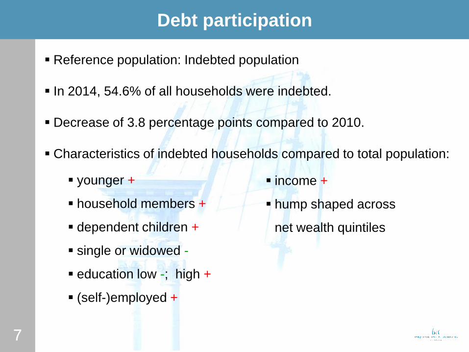
Debt participation
Reference population: Indebted population
In 2014, 54.6% of all households were indebted.
Decrease of 3.8 percentage points compared to 2010.
Characteristics of indebted households compared to total population:
younger +
household members +
dependent children +
single or widowed -
education low -; high +
(self-)employed +
income +
hump shaped across
net wealth quintiles
8 8
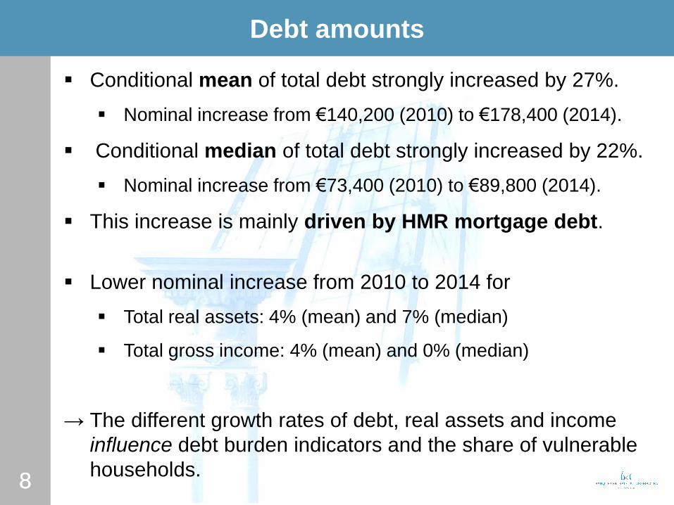
Debt amounts
Conditional mean of total debt strongly increased by 27%.
Nominal increase from €140,200 (2010) to €178,400 (2014).
Conditional median of total debt strongly increased by 22%.
Nominal increase from €73,400 (2010) to €89,800 (2014).
This increase is mainly driven by HMR mortgage debt.
Lower nominal increase from 2010 to 2014 for
Total real assets: 4% (mean) and 7% (median)
Total gross income: 4% (mean) and 0% (median)
→ The different growth rates of debt, real assets and income
influence debt burden indicators and the share of vulnerable
households.
9 9
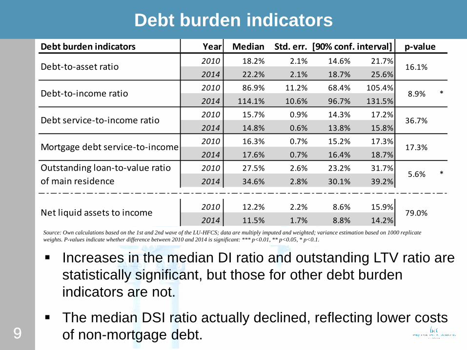
Debt burden indicators
Source: Own calculations based on the 1st and 2nd wave of the LU-HFCS; data are multiply imputed and weighted; variance estimation based on 1000 replicate
weights. P-values indicate whether difference between 2010 and 2014 is significant: *** p<0.01, ** p<0.05, * p<0.1.
Increases in the median DI ratio and outstanding LTV ratio are
statistically significant, but those for other debt burden
indicators are not.
The median DSI ratio actually declined, reflecting lower costs
of non-mortgage debt.
Debt burden indicators Year Median Std. err. p-value
2010 18.2% 2.1% 14.6% 21.7%
2014 22.2% 2.1% 18.7% 25.6%
2010 86.9% 11.2% 68.4% 105.4%
2014 114.1% 10.6% 96.7% 131.5%
2010 15.7% 0.9% 14.3% 17.2%
2014 14.8% 0.6% 13.8% 15.8%
2010 16.3% 0.7% 15.2% 17.3%
2014 17.6% 0.7% 16.4% 18.7%
2010 27.5% 2.6% 23.2% 31.7%
2014 34.6% 2.8% 30.1% 39.2%
2010 12.2% 2.2% 8.6% 15.9%
2014 11.5% 1.7% 8.8% 14.2%
[90% conf. interval]
16.1%Debt-to-asset ratio
Debt-to-income ratio 8.9% *
36.7%Debt service-to-income ratio
Mortgage debt service-to-income ratio
Outstanding loan-to-value ratio
of main residence
Net liquid assets to income 79.0%
5.6% *
17.3%

10 10
Debt burden indicators across HH characteristics
Median regression to quantify the correlation between debt
burden indicators and household characteristics.
Focus on wave 2.
Summary:
Net wealth correlates negatively with most debt burden
indicators (except the DSI ratio).
Low income households are also those with the lowest
median leverage.
Debt is lower among households where the financially
knowledgeable person is older.
11 11
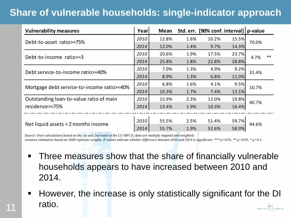
Share of vulnerable households: single-indicator approach
Source: Own calculations based on the 1st and 2nd wave of the LU-HFCS; data are multiply imputed and weighted;
variance estimation based on 1000 replicate weights. P-values indicate whether difference between 2010 and 2014 is significant: *** p<0.01, ** p<0.05, * p<0.1.
Three measures show that the share of financially vulnerable
households appears to have increased between 2010 and
2014.
However, the increase is only statistically significant for the DI
ratio.
Vulnerability measures Year Mean Std. err. p-value
2010 12.8% 1.6% 10.2% 15.5%
2014 12.0% 1.4% 9.7% 14.3%
2010 20.6% 1.9% 17.5% 23.7%
2014 25.8% 1.8% 22.8% 28.8%
2010 7.0% 1.3% 4.9% 9.2%
2014 8.9% 1.3% 6.8% 11.0%
2010 6.8% 1.6% 4.1% 9.5%
2014 10.3% 1.7% 7.4% 13.1%
2010 15.9% 2.3% 12.0% 19.8%
2014 13.4% 1.9% 10.3% 16.4%
2010 55.5% 2.5% 51.4% 59.7%
2014 55.7% 1.9% 52.6% 58.9%94.6%Net liquid assets < 2 months income
70.0%
4.7% **
31.4%
10.7%
40.7%
Debt-to-asset ratio>=75%
[90% conf. interval]
Debt-to-income ratio>=3
Debt service-to-income ratio>=40%
Mortgage debt service-to-income ratio>=40%
Outstanding loan-to-value ratio of main
residence>=75%
12 12
Cumulative distribution of debt burden indicators (1)
Source: Own calculations based on the 1st and 2nd wave of the LU-HFCS; data are multiply imputed and weighted;
the cumulative distribution functions are calculated and displayed for each implicate separately for 2014 (red) and 2010/11 (blue).
13 13
Cumulative distribution of debt burden indicators (2)
Moderate changes in the thresholds around conventional
levels would not generally produce significant changes in the
share of vulnerable households.
Exception is the NLAI ratio: small change in the threshold
makes a difference.
Conventional threshold for the NLAI ratio nearly cuts the
population in half, while for the other indicators the
conventional threshold usually cuts off only 10-20% of the
population in the tail of the distribution.
Cumulative distributions in 2010 and in 2014 do not differ
much.
Moderate changes in thresholds would not much affect the
share of vulnerable households from 2010 to 2014.
Exception is the outstanding LTV ratio.

14 14
Share of vulnerable households: multiple-indicator approach
Source: Own calculations based on the 1st and 2nd wave of the LU-HFCS; data are multiply imputed and weighted.
The rows on the DSI ratio refer to all indebted households. The rows on the MDSI ratio refer only to households with mortgage debt on their main residence.
Focus on those vulnerable households that represent a
risk of losses for the lender.
Identify households that meet several conditions:
→ Relative increase in the share of vulnerable households
is more sizable but still not statistically significant.

15 15
Distribution of households by multiple-indicators
Source: Own calculations based on the 1st and 2nd wave of the LU-HFCS; data are multiply imputed and weighted.
The upper panel on the DSI ratio refers to all indebted households. The figures in the bottom row provide the share of households in the respective category.
45.8%
45.1%
36.5% 39.4%
46.4%
45.1%
44.4% 41.0%
7.9% 9.8%19.1% 19.6%
0%
10%
20%
30%
40%
50%
60%
70%
80%
90%
100%
DSI≤20% 20%<DSI≤30% 30%<DSI≤40% DSI>40%
64.1% 21.5% 7.4% 7.1%
4.3%
1.4%
49.6%
37.5%
32.2% 32.5%
43.0%
51.7%48.3% 42.8%
7.4% 10.8%19.5% 24.8%
0%
10%
20%
30%
40%
50%
60%
70%
80%
90%
100%
DSI≤20% 20%<DSI≤30% 30%<DSI≤40% DSI>40%
63.3% 19.9% 8.0% 8.9%
NLAI<2 & DA≥75%
NLAI<2 & DA<75%
NLAI≥2
6.0%
2.2%
2010 2014
Most households have moderate DSI ratios below 20% or 30%.
Share of households with NLA > 2 months income (green segment)
decreases with increasing DSI ratio.
Share of households that combine a low NLAI ratio with a high DA
ratio (red segment) increases with increasing DSI ratio.
→ Households with high DSI ratios tend to have proportionally less
favourable NLAI and DA ratios.
*
* *
*
* Refers to figures
in slide 14.

16 16
Vulnerability indicators across HH characteristics
Probit analysis to quantify the correlation between the
vulnerability indicators and household characteristics.
Focus on wave 2.
Summary:
Highly leveraged households and household with a high
debt servicing burden tend …
to be part of more vulnerable groups (low income &
wealth);
to be part of the less vulnerable socio-economic
groups of the population (in terms of education,
employment and HMR ownership status).

17 17
Summary
Mixed picture on the changes of household indebtedness and
financial vulnerability in LU across the two waves.
Summary statistics Across the distribution
+
Debt participation rate
decreased
Most median debt burden
indicators show no statistically
significant changes
The share of vulnerable
households does not change
significantly for most indicators
More advantaged households hold
debt
Low income households have lower
leverage than high income households
Most households have moderate DSI
ratios below 20% or 30%
Disadvantaged socio-economic
groups (in terms of education,
employment status & HMR ownership
status) tend to be less financially
vulnerable
-
Total debt increased (more than
assets and income)
Median DI ratio & outstanding
LTV ratio increased statistically
DI ratio suggests a statistically
significant increase in the share
of vulnerable households
Households with high DSI ratios tend
to have proportionally less favourable
NLAI and DA ratios
Low income and wealth increase the
probability of being identified as
financially vulnerable

Thank you!