ETH Zurich

Proseminar in Theoretical Physics

Gauge/Gravity DualityThe AdS5/CFT4 Correspondence

Coordinator:Prof. M. Gaberdiel

Supervisor:Dr. Cristian Vergu

Author:Kevin Ferreira

Abstract

The introductory point consisting of a description of ’t Hooft’s large N limitand its relation with string theory, a quick jump is then made towards theexposition of Maldacena’s argument of the AdS5/CFT4 duality. The holo-graphic principle is introduced and analysed in the context of the correspon-dence. Finally, correlation functions, in the context of the AdSd+1/CFTd,are studied for scalar fields and the simple examples are computed in detail.

Contents

1 Introduction 2

2 Large N Gauge Theories as String Theories 52.1 Double Line Notation and ’t Hooft Limit . . . . . . . . . . . . . . 52.2 Perturbative Expansion and Link with Strings . . . . . . . . . . . 6

3 D3-Branes: Gauge Theories andClassical Super-Gravity Solutions 103.1 N = 4 Super-Yang Mills U(N) Theory . . . . . . . . . . . . . . . 113.2 Classical Super-Gravity Solutions . . . . . . . . . . . . . . . . . . 12

3.2.1 Black p-Branes . . . . . . . . . . . . . . . . . . . . . . . . 133.2.2 Near Horizon Limit and Redshift . . . . . . . . . . . . . . 16

3.3 5-dimensional Anti-de Sitter Space . . . . . . . . . . . . . . . . . 173.3.1 Global Coordinates and General Features . . . . . . . . . . 173.3.2 Poincare Coordinates . . . . . . . . . . . . . . . . . . . . . 183.3.3 Boundary and Conformal Boundary . . . . . . . . . . . . . 20

4 The AdS5/CFT4 Correspondence 234.1 The Dual Descriptions . . . . . . . . . . . . . . . . . . . . . . . . 23

4.1.1 Matching of Symmetries . . . . . . . . . . . . . . . . . . . 244.1.2 Tractable Limits, Validity Regimes and Duality . . . . . . 25

4.2 Formulation of the Correspondence . . . . . . . . . . . . . . . . . 274.3 Holography . . . . . . . . . . . . . . . . . . . . . . . . . . . . . . 28

4.3.1 Matter Entropy Bound . . . . . . . . . . . . . . . . . . . . 284.3.2 The Holographic Principle . . . . . . . . . . . . . . . . . . 294.3.3 AdS/CFT and Holography . . . . . . . . . . . . . . . . . . 30

5 AdS/CFT Correlation Functions 335.1 Massless Scalar Field 2-point Function . . . . . . . . . . . . . . . 335.2 General Method for Massive Scalar Field n-point Function . . . . 37

6 Conclusion 39

1 Introduction

This document reports the presentation given on the 27th of May at ETH Zurichin the frame of the Proseminar in Theoretical Physics: Conformal Field Theoryand String Theory, coordinated by the Prof. Matthias Gaberdiel.The objective of this talk as intended by its author was to present the basicfeatures of the AdS5/CFT4 correspondence, namely:

• a brief description of the first ideas that lead to conjecture a gauge/stringduality (the ’t Hooft limit, following [1],[9])

• the emergence of the conjecture from the D3-brane dual low energy descrip-tion in terms of a maximally supersymmetric gauge theory on the world-volume and its backreaction on the geometry (following mainly [1])

• Anti-de-Sitter space and its features (following [1],[9],[2])

• a brief account for the precise statement of the strong form of the dualityand its formulation (following [2],[1])

• the realisation of the duality as a boundary-bulk relation and how hologra-phy may be incorporated (following [2])

• a brief description of the holographic ideas and their realisation in AdS/CFT(following [6],[4],[1])

• AdS/CFT correlation functions for scalar fields (following [2],[9]).

The conjecture of the AdS/CFT correspondence was first made by Juan Mal-dacena in 1997, and since then it has been subject of intense research. One of themain concerns of today ’s research on the subject is integrability, which will bebriefly accounted for towards the end of this report.

Firstly, a brief exposition of ’t Hooft’s ideas on gauge/string duality will bepresented as a hint to what may such a duality look like, and how it may beformulated. This is done via an expansion in terms of Feynman diagrams on thelarge N limit of a U(N) gauge theory, mainly following [9].

2

In this document the argument presented in [1] is followed intending to con-jecture the duality between Type IIB String Theory in AdS5×S5 and N = 4U(N) gauge theory in M1,3 Minkowski space. In this argument, the low energydescription of D3-branes as classical p-dimensional supergravity solutions (blackp-branes) in 10-dimensional type IIB string theory and their dual description asa N = 4 Super-Yang Mills gauge theory in the 4-dimensional world-volume witha 10-dimensional type IIB string theory in the bulk, play a fundamental role1.Indeed, it is the analysis of a stack of N D3-branes in a low energy limit in bothdescriptions that allows the conjecture to relate a gravity-including string theoryin a non-trivial background created by the stack and the gauge theory living inthe stack world-volume itself.

Among these considerations, a brief presentation of the 5-dimensional Anti-deSitter space (AdS5) will be given. This will be done by considering the usualdescription of AdS5 as a hypersurface in M2,4 6-dimensional Minkowski space. Abrief account for different patches will be given, emphasising the Poincare patch,which is the one naturally arising when considering the near-horizon limit of theD3-branes geometry.

Supported by this, the strong form of the conjecture is made and a briefaccount of its consequences and first matches is done. In particular, the symmetrygroups of both theories are compared (the bosonic subgroup only), and certaintractable regimes are briefly studied. Also, the correspondence is seen to berealised in terms of a boundary-bulk formulation where the bulk string fieldscouple as sources of boundary CFT local operators (as given in [2]), allowing foran explicit computation of correlation functions. This will be done in the finalchapter of this report for the case of a massless scalar field, following [2], andthe result for the massive case will be presented. Then, the general perturbativemethod to compute n-point correlation functions is exposed, as given in [9], andbulk-to-bulk propagators are introduced. With this the exposition of the subjectends, as well as the report.

Before the final chapter, a small detour on the holographic principle and itsbasic arguments is done; then, this principle is seen to be realised explicitly inthe context of the AdS5/CFT4 correspondence, as in [1] and [2], with the usualregularised-boundary techniques.

I would like to thank Cristian Vergu for all his help as a supervisor of this workand good hints for the presentation, as well as Prof. Gaberdiel for the opportunityof working on this subject.

1This duality of descriptions was first conjectured in Polchinski, Dirichlet-Branes andRamond-Ramond Charges, hep-th/9510017v3.

3

Figure 1: The AdS5/CFT4 correspondence. The duality allows in principle tosolve theories in hard regimes using the dual theory in a soft regime. The linkbetween the different regimes between the theories is made by the use of therelation on the bottom of the figure, issued from the black p-brane calculations.

4

2 Large N Gauge Theories as String Theories

In this section, we follow [9] on the analysis first made by ’t Hooft of large Ngauge theories with gauge group U(N). This analysis proceeds by considering aperturbative 1/N expansion in terms of Feynman diagrams with a slight change innotation with respect to the usual Yang-Mills notation. It will be seen explicitlythat for vacuum bubbles made up of adjoint fields this leads to an expansionin topological triangulations where topologies are suppressed by N−2g factors,where g is the genus. The main contributions are therefore given by sphere-triangulations, i.e. planar graphs. This corresponds to the usual closed interactingstrings gs expansion in terms of worldsheet topologies.

2.1 Double Line Notation and ’t Hooft Limit

Consider a U(N) Yang-Mills gauge theory with gauge fields Aaµ in the adjointrepresentation, coupling constant gYM and some general Lmatter part of the La-grangian composed of matter fields. Write the Lagrangian density in the usualform as

L =1

g2YM(Tr(FµνF

µν) + Lmatter) , (1)

where the field strength is given by Fµν = ∂µAν − ∂νAµ + igYM [Aµ, Aν ].

Define the ’t Hooft parameter to be λ ≡ g2YMN . The ’t Hooft limit is definedas letting N →∞ while keeping λ fixed. It is possible to see that the Lagrangiandensity goes as L ∼ N/λ, and this will be used later.

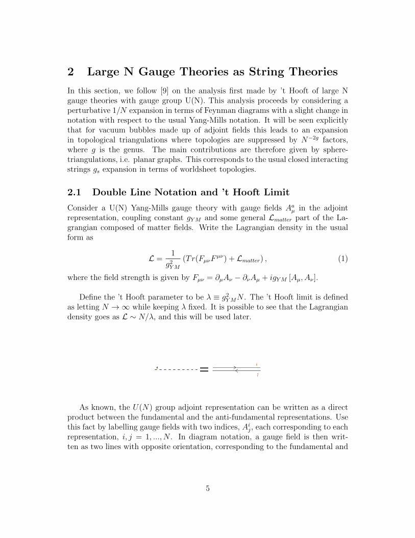
As known, the U(N) group adjoint representation can be written as a directproduct between the fundamental and the anti-fundamental representations. Usethis fact by labelling gauge fields with two indices, Aij, each corresponding to eachrepresentation, i, j = 1, ..., N . In diagram notation, a gauge field is then writ-ten as two lines with opposite orientation, corresponding to the fundamental and

5

anti-fundamental representations indices2, as in the figure above.

In this way, the Feynman graphs used when performing perturbative expan-sions on this theory will be networks of double lines, if only the gauge fields areconsidered, by the form of the gauge fields propagator:

〈AijAkl 〉 ∝ δilδkj .

The figure below is the diagram corresponding to the gauge field self-energy, inthe usual and new notations.

Figure 2: Gluon field self-energy, as in [9].

This diagram is of order O(g2YMN), as each propagator contributes with afactor g2YM , each 3-gluon vertex with g−1YM and the loop index runs between Npossible values. In the ’t Hooft limit, this diagram receives therefore no divergentcontributions.

2.2 Perturbative Expansion and Link with Strings

Keeping in mind the form of the Lagrangian as

L =N

λ(Tr(FµνF

µν) + Lmatter) ,

it is easy to derive a set of Feynman rules that allows to write the contributionsgiven by connected vacuum diagrams of gauge fields.

By the considerations given before, these graphs can be seen as correspond-ing to compact, closed, oriented surfaces. One useful way of understanding thisfact is by considering the double line diagrams as topological simplicial triangula-tions. In the figure below this is explained for two different vacuum bubble graphs.

2Each line is made to correspond to an index, and not to a field as usual in quantum fieldtheories

6

Figure 3: Some graphs in the double line notation, as in [9].

The Feynman rules read:

• N/λ for each vertex (V)

• λ/N for each propagator (E, edge)

• N for each loop (F, face)

where edge is used to denote propagators as it corresponds to the object connectingtwo vertices, and face is used to denote loops as it corresponds to a successionof propagators/edges that close on themselves with no propagators/edges inside.Therefore each graph contributes with

NV+F−EλE−V = NχλE−V , (2)

where χ is Euler’s characteristic of the 2-dimensional surface represented by thegraph. For closed oriented surfaces we can write χ = 2 − 2g, with g the surfacegenus. The sum over all Feynman graphs therefore takes the form

∑g fixed

∞∑g=0

N2−2gfg(λ) =∑

g fixed

∞∑g=0

(1

N

)2g

N2fg(λ),

and the ’t Hooft limit corresponds to a perturbative expansion in even negativepowers of N . This means that higher genus surfaces are suppressed by factors of

7

N−2g and therefore the leading contributions come from planar graphs that havethe topology of a sphere g = 0. Remark that no assumption is made about howto sum over all graphs of a given genus, but the conclusion remains.

This corresponds remarkably to the closed string perturbative gs expansion inworldsheet topologies, with the identification gs ∼ 1/N . This expansion arises instring theory when considering closed oriented strings interactions by summingnot only over possible worldsheet metrics but also possible topologies. We havethen

Sstring = SPolyakov + φχ, χ =1

4π

∫d2σ√gR,

and by Gauss-Bonnet theorem χ is just Euler’s characteristic, a topologicallyinvariant number for 2-dimensional surfaces. When summing over possible world-sheet topologies, gs ≡ eφ plays the role of a coupling constant and the sum maybe seen as a perturbative expansion.

Figure 4: String interactions and topological expansion.

To compute connected n-point correlation functions for some operators Oj

consider the transformed action3 S → S + N∑

j JjOj, for any arbitrary sourcesJj, and write in the ’t Hooft limit

〈n∏j=1

Oj〉 = (iN)−n

δnWn∏j=1

δJj

Jj=0

∝ N2−n, (3)

where W is the generating functional of connected graphs. It is remarkable to seethat 2-point functions come out canonically normalised and 3-point functions areproportional to 1/N , so that indeed in this limit 1/N is the coupling constant.One can easily be convinced that the addition of matter fields in the fundamen-tal representation of U(N) corresponds to the effect of open strings. Indeed, as

3For consistency the additional term is made to scale in the same way as the first originalterm in the ’t Hooft limit.

8

fundamental fields carry only one index, in our notation they would correspondto the presence of boundaries in the surfaces representing the Feynman diagramexpansion. Then again the expansion would be made in terms of the Euler’s char-acteristic χ = 2− 2g − b, where b is the number of independent boundaries, andit would correspond to a gs string theory expansion, for both open and closedstrings. Remark that now, contrary to the previous case, the expansion containsterms in odd powers of 1/N .

It is finallly important to take away from this section that it is possible to ob-tain a similar treatment as the one obtained in standard string theory by analysinga special limit in a gauge theory. It has not been treated, and this method does notprovide it, any way of explicitly deriving such possible correspondence betweenthe two theories, this is rather the purpose of the AdS/CFT.

9

3 D3-Branes: Gauge Theories and

Classical Super-Gravity Solutions

This section introduces a paradigm that is central to the AdS/CFT correspon-dence. This paradigm is a dual description of a stack of N D3-Branes, which willthen lead to the gauge/gravity duality of the correspondence.

In a first part a description of the gauge theory living in the world-volume ismade, with an emphasis on its symmetries. Indeed, in a low energy limit whenN parallel D-branes are made to coincide, the usual U(1) gauge theory living oneach brane enhances the system’s gauge symmetry from U(1)N to U(N). In thisprocess enter the Chan-Paton factors, which label the brane on which each end ofthe strings live, and that in the end become the indices of the final gauge group.The gauge theory surviving in the D3-branes world-volume inherites the space-time supersymmetry of type IIB string theory, but not fully as D-branes breakhalf the supersymmetries. Therefore, this gauge theory contains 16 conserved su-percharges; being a 4-dimensional theory, it is constrained to have supersymmetryrank N = 4. The Lagrangian of this theory is completely settled by these consid-erations and the final unique theory is called N = 4 Super-Yang Mills theory.

In a second part of the section, same system of N D3-branes is again describedbut using a different analysis. Given the natural emergence of gravity from stringtheory, and D-branes being charged massive objects in this theory, the questionnaturally arises of knowing what is the geometric meaning of a stack of D-branes.In particular, using the low energy limit of superstring theory, namely super-gravity, it is possible to replace the D-branes influence on the theory by a non-trivial geometry4 and let strings react to this non-trivial background. This is muchin the same way as a very familiar dicotomy in physics, which can be grasped byconsidering the example of an electron-proton scattering process. Indeed, thereare two different ways of describing this process, at least in a low energy limit.The first one is by considering and summing over all possible Feynman diagramsthat contribute to the process, find an expression for the S-matrix using the usualQED methods and obtaining a scattering amplitude. The second is to considerthat the proton creates a static electric field in its surroundings and that theelectron reacts to this non-trivial space by scattering through it5, i.e. by beingfree in a deformed background and interacting with it. This is indeed the perfectanalogy of what will be done when describing the N D3-branes by its geometrybackreaction.

4In opposition to the usual flat 10-dimensional background considered in superstring theory5Taking the simplistic and helpful consideration that the proton does not move.

10

3.1 N = 4 Super-Yang Mills U(N) Theory

As discussed, the theory living on the world-volume of a stack of D3-branes in alow energy limit is a supersymmetric non-abelian gauge theory N = 4 with gaugegroup U(N).This theory contains the following fields:

• λaα, α = 1, 2, a = 1, ..., 4 left Weyl fermionic fields

• X i, i = 1, ..., 6 real scalar fields - SO(6) ∼ SU(4)

• Fµν = ∂µAν − ∂νAµ + i [Aµ, Aν ], Aµ gauge fields with field strength Fµν

• Dµλ = ∂λ+ i [Aµ, λ], a covariant derivative.

The 6 real scalar fields X i transform between themselves by a SO(6) rotation,which appears from the breaking of Lorentz symmetry by the D3-branes, namelySO(1, 9) −→ SO(1, 3)×SO(6), the first part being related to the fields tangent tothe D3-branes that live in a theory with Lorentz symmetry in the world-volume,and the second part representing the transversal dynamics, the fields X i labellingthese type of excitations of the branes.

The Lagrangian is completely settled by supersymmetry:

L = Tr

(− 1

2g2FµνF

µν +θI

8π2FµνF

µν −∑a

iλaσµDµλa

−∑i

DµXiDµXi +

∑a,b,i

gCabi λa

[X i, λb

]+∑a,b,i

gCiabλa[X i, λb

]+g2

2

∑i,j

[X i, Xj

]2),

where F µν = εµνρσFρσ is the dual field strength and θI is the instanton angle. The

constants Cabi are Clebsch-Gordon coefficients relating fields of different spins and

the Yang Mills coupling g is related to the string coupling by g2 ∼ gs.

The details of this theory, including the consequences of such Lagrangian den-sity, are not of fundamental importance in the context of this report, except forthe few following points. Firstly, it can be seen by dimensional analysis that

11

Figure 5: The brane modes composing N = 4 SYM and low energy limit describ-ing the bulk modes, 10d supergravity.

this theory is renormalisable. But this isn’t all, it can be shown that the theoryhas a vanishing β-function. This means that this theory is actually a ConformalField Theory, or CFT. Also, it preserves all its symmetries at the quantum level,namely:

• R-symmetry SO(6) ∼ SU(4), with 15 traceless hermitian generators T ab, a, b =1, ..., 4

• conformal symmetry in 4d SO(2, 4) with generators Pµ, Lµν , D,Kµ

• N = 4 Poincare Supersymmetry

These symmetries compose the superconformal group SU(2, 2|4) of this gaugetheory, and the superalgebra may be represented by a diagonal bosonic part andan off-diagonal fermionic part: Pµ, Kµ, Lµν , D Qa

α, Saα

Qαa, Sαa T ab

where Qa

α, Qαa are the usual supersymmetry generators and Sαa, Saα are the gen-

erators given by the commutation relations of Qaα, Qαa with the special conformal

transformations Kµ, and that therefore close the algebra.

3.2 Classical Super-Gravity Solutions

Historically this subject didn’t develop as presented in this report. In fact, theconjecture of the D-branes existence was proposed in parallel of the discovery of

12

the black p-brane solution of supergravity that is exposed here. It was only in1995 that J. Polchinski conjectured the duality of the description, i.e. that infact this solution corresponds to D-branes6. The exposition made in this reportis based in a full aknowledgement of this conjecture.

3.2.1 Black p-Branes

As known, Dp-branes are massive charged objects. Consider the classical super-gravity action

S =1

(2π)7α′4

∫d10x√−g(e−2φ(R + 4(∇φ)2)− 2

(8− p)!F 2p+2

), (4)

where Fp+2 = dAp+1 is the field strength associated to a Ap+1 potential obtainedin superstring theory. In the case of interest here, type IIB string theory, there area 2-rank tensor and a 4-rank tensor resulting from the theory, i.e. p = 1, 3. Thecase which corresponds to D3-branes, p = 3, which will be detailed in this report,corresponds to the 4-rank tensor in the Ramond-Ramond sector of superstringtheory, with self-dual field strength F5 = ∗F5

7.

Look for a p-dimensional solution carrying N charges8 with respect to thispotential9

N =

∫S8−p∗Fp+2,

and require some desirable symmetries: euclidean symmetry ISO(p) in p dimen-sions along the Dp-branes, and spherical symmetry SO(9-p) in the (9-p) transver-sal directions.

This reduces the problem to the finding of a spherically symmetric chargedblack hole static solution in (10-p) dimensions. In general relativity this corre-sponds to the Reissner-Nordstrom solution of a static, charged black-hole. In thiscase, the situation is more complex but the solution has some similarities:

ds2 = − f+(ρ)√f−(ρ)

dt2 +√f−(ρ)

p∑i=1

dxidxi +f−(ρ)−

12− 5−p

7−p

f+(ρ)dρ2 +ρ2f−(ρ)

12− 5−p

7−pdΩ28−p,

(5)

6In Dirichlet-Branes and Ramond-Ramond Charges, November 1995, arXiv-hep-th/9510017v3

7This condition has actually to be added to the action (4), as it is not implied by it.8Each Dp-brane carries one unit of charge.9The dimension of the world-volume of the object and the rank of the potential coincide, as

required by a minimal coupling.

13

where

f± = 1−(r±ρ

)7−p

,

and the parameters r± are related to the mass and charge of the N Dp-branes by

M =1

(7− p)(2π)7dpl8P

((8− p)r7−p+ )− r7−p−

), (6)

N =1

dpgsl7−ps

(r+r−)7−p2 . (7)

Here ρ is the radial direction in the (9-p) spherically symmetric submanifold,and the xi parametrise the Dp-branes. The symbol lP is Planck’s constant in 10dimensions and dp is the area of the unit (p-1)-sphere.

It is possible to see that there is a horizon at ρ = r+. Indeed, use the metricto compute

g

(∂

∂t,∂

∂t

)= − f+(ρ)√

f−(ρ)= 0 at ρ = r+.

Also, for p ≤ 6, there is a curvature singularity at ρ = r−. It is possible tosee it by computing some frame-invariant quantity, as the Kretschmann scalarK = RµνρσR

µνρσ, and see its divergence when ρ = r−. This is done in the sameway, and yielding a similar result, as in simpler Schwarzschild solution.

By the cosmic censorship hypothesis, which states that no naked singularitiesshould exist10, it is imperative to have r+ ≥ r−. This implies a lower bound tothe mass, using (7) and (6),

M ≥ N

(2π)7gslp+1s

.

where it has been used l4P = gsl4s . For supersymmetry reasons11 we retain the

solution with r+ = r− ≡ R , called the extremal solution, where the horizon andthe curvature singularity are made to coincide. All care is necessary to treat thiscase as the supergravity description becomes inadequate at a certain distance ofthe singularity, as the curvature becomes too high. For the case p=3, which willbe the case in interest, the situation is nevertheless more gentle as the ρ = r+surface is regular and it is possible to find a smooth analytic extension of thesolution. Writing everything in this extremal case, the solution (5) becomes

10This is usually linked to the requirement of having a well-posed Cauchy problem.11The found inequality is related to the BPS bound with respect to the 10 dimensional space-

time supersymmetry.

14

ds2 =√f+(ρ)

(−dt2 +

p∑i=1

dxidxi

)+ f+(ρ)

32− 5−p

7−pdρ2 + ρ2f+(ρ)12− 5−p

7−pdΩ28−p, (8)

where now

f+(ρ) = 1−(R

ρ

)7−p

.

The symmetry ISO(p) is enhanced to the Poincare symmetry ISO(1,p), whichis rather pertinent as theories in Dp-branes should carry this kind of spacetimesymmetry in the limits which are of interest to us. Using equation (7) in theextremal case, it is possible to get an expression for R:

R7−p = dpgsl7−ps . (9)

Define a new coordinate r7−p = ρ7−p−R7−p; notice that the horizon is now atr = 0. Also, define H(r) = [f+(ρ(r))]−1:

H(r) =1

1−(Rρ

)7−p =1

1− R7−p

r7−p+R7−p

=r7−p +R7−p

r7−p= 1 +

(R

r

)7−p

.

Focus on the p=3 case, corresponding to D3-branes. Then using

d(ρ4) = d(r4) =⇒ dρ2 =

(r3

ρ3

)2

dr2 =r6dr2

(r4 +R4)3/2

=⇒ dρ2 =1

(1 + R4

r4)3/2

dr2 = H(r)−3/2dr2,

and also ρ2 = (r4 +R4)1/2 = r2H(r)1/2, the solution (8) reads

ds2 =1√H(r)

ηµνdxµdxν +H(r)2H(r)−3/2dr2 + r2H(r)1/2dΩ2

5

=⇒ ds2 =1√H(r)

ηµνdxµdxν +

√H(r)(dr2 + r2dΩ2

5). (10)

Before continuing, it is useful to remark that this supergravity description isadequate in a low curvature limit, i.e. when R ls. Using the relation

R4 = 4πNgsl4s , (11)

15

obtained from (9) by using d3 = 4π, it is easy to conclude that this description isvalid when

1 gsN N, (12)

where the last relation arises from the fact that we are always implicitly consider-ing gs to be small and a perturbative expansion on gs to be meaningful. Thereforeby this relation this is also a large N limit of the system12.

It is interesting, as well as fundamental, to remark that this decription is dualto the one obtained in the previous section via a gauge theory in the world-volumeof the D3-branes. Indeed, a perturbative treatment of this gauge theory is compre-hensible and meaningful when the effective parameter is small enough, i.e. whengsN 1. This is perfectly incompatible, and thus dual, with the regime found in(12). This is a central statement to the gauge/gravity duality.

3.2.2 Near Horizon Limit and Redshift

In the next chapter the near horizon limit of this geometry will be needed. Asalready mentioned, the horizon is at r = 0, so that a meaningful limit to takenear the horizon is r/R 1. In this limit,

√H(r) =

√1 +

R4

r4=R2

r2

√r4

R4+ 1 ' R2

r2,

and therefore the solution represents a geometry which in this limit is

ds2 =r2

R2ηµνdx

µdxν +R2

r2dr2 +R2dΩ2

5. (13)

This is the metric of the product space of 5-dimensional Anti-de Sitter spacewith a 5-dimensional sphere, AdS5×S5, both with radius R. The 5-sphere is trivialto see in this solution, as it constitutes the third term. For those unfamiliar withAnti-de Sitter space, the next subsection should be useful to clarify this aspect.

Another important aspect of this geometry is the redshift it produces. Considertwo observers (r, t) and (r′, t′), describing some line element such that

ds2 = ds′2 =⇒ −dt2√H(r)

=−dt′2√H(r′)

12It is evident that it is easier to treat the system when the number N of D-branes, and thusthe total charge and mass, are large, since in this way it is easier to clear-cut it from quantuminfluences.

16

=⇒ dt′

(H(r′))1/4=

dt

(H(r))1/4.

Send one of the radial coordinates to infinity, so that H(r) ' 1, and remark that

there will be an associated redshift [H(r)]−1/4. Since the redshift goes to zerowhen r −→ 0, i.e. near the horizon, an observer at infinity see states in thisregion as having a very low energy no matter the energy the state has in thestring frame. This will be important to keep in mind in the next section.

3.3 5-dimensional Anti-de Sitter Space

Anti-de Sitter space has a variety of descriptions, one of the most interesting onesbeing that it is a maximally symmetric13 solution to Einstein field equations witha negative cosmological constant. Nevertheless, for the sake of brevity and objec-tivity, the description used here is the one of a 5-dimensional hypersurface in a2+4-dimensional Minkowski space.

Consider for that matter the metric in M2,4 in cartesian coordinates (xi)5i=0

ds2 = −dx20 − dx25 +4∑i=1

dx2i ,

and the hypersurface given by

x20 + x25 −4∑i=1

x2i = R2,

for some real positive R2.

3.3.1 Global Coordinates and General Features

Introduce a new set of coordinates (τ, ρ,Ωi), ρ ≥ 0, τ ∈ [0, 2π), defined by

x0 = R cosh ρ cos τ, x5 = R cosh ρ sin τ

xi = R sinh ρ Ωi, i = 1, ..., 4 :∑i

Ω2i = 1,

that solve the quadric equation defining AdS5. Then

dx20 = R2 (sinh ρ cos τ dρ− cosh ρ sin τ dτ)2

13Carrying the same number of isometry generators as Euclidean space.

17

dx25 = R2 (sinh ρ sin τ dρ− p+ cosh ρ cos τ dτ)2

dx2i = R2 (cosh ρ Ωi dρ+ sinh ρ dΩi)2 .

Substituting this results in the Minkowski metric, and carrying the computationusing trigonometric identities and

ΩiΩi = 1 =⇒ ΩidΩi = 0,

it is possible to find the intrinsic metric of the AdS5 hypersurface:

ds2AdS = R2(dρ2 + sinh2 ρ dΩ2

i − cosh2 ρ dτ 2).

These are called the global coordinates. Two things should be remarked by the useof these coordinates: first, the time coordinate is 2π-periodic. This unpleasantfeature can be discarded by unwarping the τ coordinate to −∞ < τ <∞ withoutany identifications. By this means the result is the universal cover of AdS5, andthis is what will be used throughout this report. Secondly, at ρ ∼ 0 the metricreads

ds2AdS ' R2(dρ2 + ρ2 dΩ2i − dτ 2)

which indicates that AdS5 is isomorphic to a cylinder S1 × R4, as τ is periodic.

Figure 6: Anti-de Sitter as a hypersurface in Minkowski space, in global coordi-nates.

3.3.2 Poincare Coordinates

To get the form of the metric found in the near horizon region in the last sub-section, a new set of coordinates (u, ~x, t), called Poincare coordinates, must beused:

x0 =1

2u(1 + u2(R2 + ~x2 − t2)), x5 = R u t

18

x4 =1

2u(1− u2(R2 − ~x2 + t2)), xi = R u xi.

In this new patch the differentials read

dx0 =([−x0u

+R2 + ~x2 − t2]du− ut dt+ uxi dxi

)dx5 = Rt du+Ru dt

dxi = Rxi du+Ru dxi

dx4 =([−x4u−R2 + ~x2 − t2

]du− ut dt+ uxi dxi

).

Inserting these results on the metric and using the easily confirmed and helpfulresults

−x20 + x24 = −R2

u2(−t2 + ~x2 + u2

),

andx0(~x

2 − t2) + x4(t2 − ~x2) = u2R2(~x2 − t2),

one easily finds in a first computation

−dx20 + dx24 = −R2

u4(−t2 + ~x2 − u2)du2 − 2R2(uxi dxidu− ut dtdu),

and

−dx25 + dx21 + dx22 + dx23 = −R2t2 du2 −R2u2 dt2 − 2R2tu dudt+R2x2i du2

+R2u2 dx2i + 2R2xiu dudxi.

Therefore it is straightforward to see that

ds2AdS =R2

u2du2 + u2R2ηµνdx

µdxν ,

where the Lorentz notation is here used to specify the four-vector (t, ~x).This is the metric of AdS5 expressed in the Poincare coordinates, but it is not yetthe result found in (13). To find it, define

r = R2u, dr = R2du,

so that

ds2AdS =R2

r2R4dr

2

R4+r2

R4R2ηµνdx

µdxν

=⇒ ds2AdS =R2

r2dr2 +

r2

R2ηµνdx

µdxν ,

which is exactly the first two terms in (13). Remark that u has dimension(lenght)−1 so that r is a length coordinate, as R has dimension (length)1

19

3.3.3 Boundary and Conformal Boundary

Introduce a new change in coordinates by z = u−1. Then dz2 = u−4du2 and theAdS metric reads

ds2AdS = R2z2z−4dz2 +R2

z2ηµνdx

µdxν = R2 dz2 + ηµνdx

µdxν

z2. (14)

The boundary of AdS is placed on the limit r −→∞, i.e. u −→∞ or z −→ 0.The horizon, on the other hand, as seen is at r −→ 0, i.e. u −→ 0 or z −→∞.

Using this coordinate patch, it is possible to compute the time needed for alight-ray to travel radially to the boundary. First, see that

0 = ds2 =R2

u2du2 − u2R2dt2 =⇒ du

u= udt.

Integrate from some region in spacetime u = a, a 6= 0 so that it is not at thehorizon (from where it cannot escape), to the boundary u =∞ to get

∆t =

∫ ∞a

u−2du <∞.

The light ray can reach the boundary at a finite time, and therefore each point inAdS is in causal contact with the boundary of the space. This is a very specialfeature, clearly not present in Minkowski space; it becomes important to knowwhat the boundary of AdS5 looks like. To do that, there are at least two basicconstructions, which are presented in the following.

Consider the AdS5 metric above; perform a Wick rotation t −→ itE so thatthe Minkowski part of the metric becomes euclidean in the coordinates (tE, ~x).Now change the names of the coordinates to something more familiar, x0 = z,x4 = tE. Then the metric is

ds2AdSE =1

x20

4∑i=0

dx2i . (15)

These coordinates are called half-plane coordinates as in two dimensions itdescribes the half-plane z ∈ C : Im(z) > 0 with Poincare metric as given above.The half plane can be mapped to a ball in euclidean space, as in the figure below in2-dimensions, where the hole |z| =∞ is mapped to a point u = 0 in the boundaryof the ball.

The boundary u = ∞ is a 4-sphere with one point removed; this is preciselythe result of the compactification of 4-dimensional Euclidean space R4. Perform

20

Figure 7: Mapping AdS2 to a disc, as in [1].

the Wick rotation again to get the initial AdS space and finally the conclusion isthat the conformal boundary of AdS5 is compactified Minkowski space M4. Es-cher’s painting on the title page of this report is a visualisation of this feature ofhyperbolic spaces.

The second, more precise, way of seeing this is by considering the problem interms of quadrics. Start with a set of coordinates (u, v, xi) in M2,4 and considerthe quadric equation

uv − ηijxixj = 0. (16)

This quadric is invariant under an overall rescaling u −→ su, v −→ sv,xi −→ sxi. Use this scaling to fix v = 1 and solve for u

u = ηijxixj.

This parametrises the portion of the quadric with v 6= 0, not taken into account inthe previous considerations. So the quadric describes a parametrisation of (3+1)dimensional Minkowski space plus some points ”at infinity” v = 0. This is pre-cisely what is obtained from a compactification of Minkowski space.Indeed, it is analogous to the euclidean case; take for example the compactifica-tion of the real line into a circle. We may use the stereographic projection as amap from every point in the real line to every point in the circle, except the poleP. This point P would correspond to a ”point at infinity” in the real line. The fullcircle can be obtained by this procedure simply by adding this point P and de-manding that every sequence (xn) ⊂ R such that xn −→ ∞ when n −→ ∞, nowin the circle satisfies xn −→ P when n −→ ∞, thus closing the compactification

21

completely.

Figure 8: Compactification of the real line into a circle.

Use the same coordinates to write14 AdS5 as

uv − ηijxixj = 1.

Let u, v, xi −→ ∞ and do a conformal transformation by dividing by a positiveconstant factor, so that the right-hand side can be neglected and the quadric(16) is obtained. Then this quadric, the compactification of M4, is the conformalboundary of AdS5.

14Set R = 1.

22

4 The AdS5/CFT4 Correspondence

In this section the results of the previous sections are taken in order to formu-late the correspondence. The strong form of the conjecture is suggested, andits formalisation is made using the previous results on the conformal boundary ofAdS. Finally, the holographic principle is derived from black hole thermodynamicsconsiderations and its realisation in the AdS/CFT correspondence is analysed.

4.1 The Dual Descriptions

In the previous section it was seen that a stack of N D3-branes can be describedby the means of two very different descriptions: on the one hand we obtain N = 4Super-Yang Mills U(N) theory in the 4-dimensional world-volume. On the otherhand, we can replace the effect of the D3-branes by a non-trivial geometry whichis the manifold AdS5×S5 in the near horizon region. A closer analysis of the the-ories emerging from this dual description is the next step.

Consider the first encountered description. Taking the low energy limit, thesystem is completely described by two theories: a type IIB supergravity theoryliving in the bulk, and N = 4 U(N) SYM up to some higher derivative correctionterms. The total action has the form

S = Sbulk + Sbrane + Sint,

where the last term represents the interaction between the bulk states and thebrane states. It can be shown that these interactions are proportional to positivepowers of α′, so that if the limit α′ → 0 is taken while keeping gs, N fixed, theseinteractions vanish. Plus, Sbulk becomes type IIB free gravity and Sbrane becomespure N = 4 U(N) SYM theory. Therefore the states that survive to this limit canbe fully described by

• 10-dimensional free gravity in the bulk

• 4-dimensional gauge theory in the branes

Consider now the second description of the N D3-branes:

ds2 =1√H(r)

ηµνdxµdxν +

√H(r)(dr2 + r2dΩ2

5),

H(r) = 1 +R4

r4, R4 = 4πgsα

′2N.

23

As seen, energies are redshifted by a factor(

1 + R4

r4

)− 14, so that when taking

the low energy limit states of any mass close to the horizon r = 0 will survive.Indeed, any state sufficiently close to the horizon will have sufficiently low energyto survive to the limit. Plus, there are also the massless states away from thehorizon, and these two sets decouple from each other in the limit that is beingtaken.Again, the states that survive can be fully described by

• 10d free gravity in the bulk

• near horizon full theory

Therefore in both approaches two decoupled theories describing all states inthe prescribed limit are obtained. Remember that the near horizon region isAdS5×S5. If the two approaches are seen as different descritpions of the sameobject, as it has been conjectured until now, then this identification forces toidentify the two obtained results so that

N = 4 U(N) SYM in flat 3+1 dimensions

is ”equivalent” to

Type IIB superstring theory on AdS5 × S5.

The strong form of this conjecture applies for any value of gs and N , and is theone analysed in this report. Remark that, by fully aknowledging this correspon-dence, no reference is needed from now on to how the argument that was exposedand leads to this conjecture actually works. In this way, for example when readingtype IIB superstring theory on AdS 5×S 5, it should be read type IIB superstringtheory living in a background which asymptotically is as AdS 5×S 5.

4.1.1 Matching of Symmetries

The conjecture just made seems in a first regard to be more enigmatic than whatit turns out to be. These two theories are completely different: on one hand thereis 10-dimensional string theory, a gravity theory, in a very special spacetime. Onthe other hand, there is a U(N) gauge theory, which is, as seen, also a conformaltheory, living in a flat 4-dimensional spacetime!A first question that should be asked is whether the global symmetries of thesetwo theories match, and the answer is yes. Indeed, on the string theory side, theproduct space AdS5×S5 has isometry group SO(2, 4)×SO(6), the first being the

24

manifest isometry group of AdS5, the second rotating the 5-sphere.On the CFT side, there is a 4-dimensional conformal symmetry SO(2, 4) and aSO(6) symmetry as seen in section 3.1. So indeed, the bosonic part is seen tocoincide perfectly. In fact, the whole supersymmetric group SU(2, 2|4) matchesin both theories, the strange geometry on the string theory side being respon-sible for the breaking of half of the supersymmetries. Gauge symmetries, beingredundancies of the description, do not need to match.

4.1.2 Tractable Limits, Validity Regimes and Duality

The strong equivalence relation conjectured previously should be substantiatedwith strong evidence for it15. This is the purpose of the remaining of this report.For that, it is useful to start by considering the consequences of such correspon-dence between the two theories. The most fundamental one is that there shouldexist a map between states and fields on the AdS string side and local gaugeinvariant operators on the Yang-Mills CFT side, as well as a correspondence be-tween correlators. Indeed, the matching of observables between theories is theultimate request and a necessity for the theories to be different descriptions ofthe same theory, where these observables would take their full meaning.Even if the conjecture concerns the two complete theories, there are special limitsin which it is possible to see this correspondence somehow closer. One of theselimits is the ’t Hooft limit described in the first part of this report. As it wasseen, a large N limit of a U(N) gauge theory with λ = g2N fixed leads to a topo-logical expansion as the one found in classical string theory. In the context of thecorrespondence, the large N limit of N = 4 U(N) SYM corresponds to a genusexpansion in powers of gs in type IIB string theory.Another regime expected to have a meaningful result is an α′ expansion in typeIIB supergravity. What is the corresponding behaviour in the CFT part? Use theAdS metric in the form

ds2AdS = R2 dz2 + dxµdx

µ

z2,

and include it in the string theory non-linear sigma model

SG =1

4πα′

∫√γγmnGMN(x;R)∂mX

M∂nXN

=⇒ SG =R2

4πα′

∫√γγmnGMN(x;R)∂mX

M∂nXN

where

R2 dz2 + dxµdx

µ

z2= ds2AdS = GMNdx

MdxN = R2 GMNdxMdxN .

15In the perspective of today’s lack of a rigorous proof.

25

Keeping in mind equation (11), write R2/4πα′ =√

4πλ so that the supergravityα′ expansion corresponds now to a λ−1/2 expansion, meaningful in a large λ limit.

Issuing from the dual description decribed in the last section, the AdS/CFTcorrespondence inherits a similar dual behaviour. A perturbative analysis in theYang-Mills CFT part of the relation is meaningful when the coupling effectiveparameter g2N is small enough. Using relation (11), this is

g2N ∼ gsN ∼R4

l4s 1.

On the other hand, the classical gravity description is valid when the typical radiusof curvature R is large when compared to the string length. Again by equation(11) this means

R4

l4s∼ gsN ∼ g2YMN 1.

These validity regimes are perfectly incompatible, again we find this correspon-dence as a duality relation. Two important consequences arise from this fact: first,the duality gives the correspondence a much larger importance from a theoreticalpoint of view. Clearly, this duality is stating that it is possible to solve a stringtheory in a strongly curved background16 by easily solving a gauge theory in aperturbative expansion. Similarly, it should be possible to solve strongly coupledgauge theories17 by solving a low curvature string theory, which includes gravity.It is hard to overestimate the potential importance of such statement.

On the other hand, no rigorous proof or real test was given here, so given thiscomplete opposition of comprehensible regimes of validity a legitimate questionwould be how could this correspondence ever be tested if each side is understand-able in non-overlapping regimes. One important result would be to compare quan-tities from both theories which do not depend on the coupling/curvature radius.This is possible and has been done. Another more significant result obtained fromthe research made on this topic in the past 10 years has to do with the subjectof integrability. Briefly stated, the result obtained allows to interpolate betweenthe two regimes described above to a region where the overlapping happens andthe two theories can be directly compared. This has been done and yields verypromising confirmations of the AdS/CFT correspondence.

16Something which today is not at all obvious in a full quantum level, at least in the author’sunderstanding of it.

17Low energy QCD would be rather useful.

26

4.2 Formulation of the Correspondence

The precise formulation of the AdS/CFT correspondence may be made using theresults obtained until now. The main problem concerning this formulation is thatit should provide a link between the fields living in AdS5 and the operators in theCFT4.As seen, because of the particular form of Anti-de Sitter space, any field theoryin this spacetime needs boundary conditions on its fields for the theory to becompletely determined. This is by no means an easy problem, as boundary andpoints in the bulk are causally connected, as seen. It is possible nevertheless to usethis, together with the fact that the conformal boundary of AdS5 is compactified4-dimensional Minkowski space M4, and introduce a coupling∫

d4x φ0(~x)O(~x) (17)

in the CFT4 side, where O is a CFT operator and φ0(~x) is an arbitrary sourcefor this operator such that there exists a field φ(~x, z)18 in AdS5 with boundarycondition

φ(~x, z)|z=0 = φ0(~x).

In this way, a link between AdS-fields and CFT-operators is realised as a boundary-bulk relation, which is by all means possible with what was studied. Of course,mass dimensions should agree in the appropriate way so that expression (17) isdimensionless; also the quantum numbers with respect to the full symmetry groupof both the operator O and of the field φ should agree so that the coupling as awhole is meaningful in the theories.Since this bulk-boundary relation is also a source-operator correspondence, it isnatural to propose the following statement:

〈e∫d4x φ0(~x)O(~x)〉CFT

AdS/CFT= Zstring

AdS [φ(~x, z)|z=0 = φ0(~x)] , (18)

that is, the generating functional of O-correlation functions in the CFT sidematches the full partition function on the AdS side where the field correspondingto the operator O is solved having a specific boundary condition. In the end,when φ(~x) is solved in terms of φ0(~x), i.e. it is on-shell with respect to the actionin AdS5, both sides are functionals of φ0(~x). O-correlation functions on the CFTside may be computed by taking functional derivatives on the left hand side, andthen letting the sources vanish, as usual by the QFT path integral methods. Thisrelation then states that by computing the partition function in the AdS side andtaking functional derivatives with respect to the boundary field φ0(~x) the resultshould be the same. This will be done in the next section for a massless scalar

18The used coordinate system is the one introduced in (14) after a Wick rotation.

27

field, but this is a general proposition applicable in principle to fields of any spinand mass.

4.3 Holography

Before proceeding to take on hands the problem of computing correlation func-tions in the context of the correspondence, this section ends with one of the mostpromising and fascinating preliminary results of the AdS/CFT correspondence.This correspondence in its full form is an explicit statement about the equivalenceof two theories, one living in a 5-dimensional spacetime and the other in the usual4-dimensional Minkowski spacetime, on the boundary of the first as seen. Thisequivalence apparently reduces the dimension of the spacetime where the descrip-tions take its forms by 1 without any further problems. But this mismatching ofdimensions in a boundary-bulk relation seems in a first view very problematic, asthere are degrees of freedom in the 5-dimensional theory which seem to be utterlyredundant.Throughout this section it will be seen that this is not a problem, it is even anecessity if a full quantum gravity description is ever to be obtained, by meansof the holographic principle. By the end of the section, the explicit realisation ofthis principle in the context of the AdS/CFT correspondence is fully analysed.

4.3.1 Matter Entropy Bound

Black hole thermodynamics, a subject firstly introduced by Hawking and his semi-classical analysis resulting on what is now called Hawking radiation, yields theimportant result concerning black hole entropy:

SBH =A

4GN

,

where A is the black hole’s event horizon area and GN is Newton’s gravitationalconstant. Another feature which is important for the following is the fact that theblack hole’s event horizon area is proportional to the second power of the totalmass19 of the black hole, A ∼M2. Finally, it is important to state the generalised2nd law of thermodynamics, which aknowledges black hole entropy as a part of thetotal entropy of the universe and the unitarity of the processes involving blackholes, e.g. black hole scattering. In this way, it states

dSBH+matter ≥ 0,

19The subject presented in this fashion is only concerned with static black-holes.

28

where here and hereon matter refers to non-collapsed matter systems.

Following these assumptions, consider a system composed of matter of massm and entropy Smatter and a black hole of mass M and entropy SBH ∼ A ∼ M2.Let the total system evolve in such a way that the matter enters the event horizoncreated by the black hole. Then, the total entropy before and after the collapseis given by

Sbefore = Smatter +A

4,

Safter = S ′BH ∼ A′ ∼ (M +m)2.

The generalised 2nd law requires Sbefore ≤ Safter. However, as the black hole afterthe collapsing of the in-falling matter keeps no information about its entropySmatter, but only takes its mass m to enlarge its area and thus its entropy, itis straightforward to see that there must exist an upper limit to Smatter if thegeneralised 2nd law is to be true. In other words, a large enough matter entropyfor a small enough mass would violate the 2nd law as presented.Using these considerations, Bekenstein and Susskind derived generalised matterentropy bounds by considering specific processes. In particular, by consideringthe collapse of a mass shell around a matter system in order to create a blackhole, Susskind derived what is called the spherical entropy bound

S ≤ A

4GN

,

where A is the area of the smallest volume inclosing the system. Black holessaturate this inequality, and therefore have the highest possible entropy for thegiven occupied volume.

4.3.2 The Holographic Principle

Using the thermodynamical relation S = kB lnW , it is then easy to view eS asthe number of independent quantum states compatible with certain macroscopicparameters. In a full quantum theory of nature, this corresponds to the numberof degrees of freedom of the theory. More precisely,

N ≡ #dof = log dim(H),

dim(H) = eS,

where H is the Hilbert space where the theory is formulated, so that in the endthe entropy S corresponds to the number of degrees of freedom.

29

In a standard QFT, the number of degrees of freedom is infinite. Indeed, it iscostumary to view the framework of a QFT as consisting of an harmonic oscillatorin each point in space, which yields an infinite number of degrees of freedom asa system. When regularised, e.g. to describe some quantum gravity theory, as tohave 1 d.o.f. per Planck volume, the number of degrees of freedom grows as thevolume considered. This is however in contradiction to what has been exposed,as the correct relation given by the matter entropy bound is that the entropy, i.e.the number of d.o.f., should grow as the area of the considered volume, S ∼ A.

The holographic principle is obtained by fully aknowledging the previous re-sults as a principle of nature and by generalising it to all frameworks susceptibleof describing nature. It states

In a quantum theory of gravity all physics within some volume can bedescribed in terms of some theory on the boundary which has less thanone d.o.f. per Planck area.

This principle is formulated so that every system satisfies the required entropybound. For conclusion, our usual theories have a redundacy in the form of uselessdegrees of freedom. This redundancy can be solved by considering some corre-sponding theory on the boundary of the space our theories live in. Even if statedin a purposely intended fashion so to be used in the AdS/CFT correspondence,this principle in its general form, and by what has been presented as argument toit, can be seen to have a faithful realisation in the bulk-boundary relation exposedto formulate the AdS/CFT correspondence.

4.3.3 AdS/CFT and Holography

The explicit analysis of the holographic character of the AdS/CFT correspondenceis of no trivial matter, contrary to what the explicit boundary-bulk relation maylead to think. Indeed, the CFT living on the boundary, being a field theory, hasan infinity of degrees of freedom. In the same way, the area of the boundary ofAdS space is infinite, so that in these terms a comparison between the two isimpossible.In order to be able to make such comparison, a regularisation of the 4-dimensionalboundary space has to be achieved. For that purpose, a discretisation of its spatialpart in terms of small cells of size δ 1 is made, and 1 d.o.f. is considered percell. As the total number of cells is proportional to δ−3, and the theory living onthe boundary is a U(N) gauge theory, the total number of degrees of freedom goesas

SregCFT ∼ δ−3N2. (19)

30

This UV cut-off introduced in the boundary relates to the bulk AdS theoryby imposing a IR cut-off. This is part of a broader subject usually refered to asIR-UV connection. It can be seen by considering a string stretching in the bulkto a point in the boundary. In the boundary theory, it will be seen as a pointparticle, and being charged it yields a divergent self-energy. This can be solvedin the CFT context by imposing a UV cut-off to regularise these divergences. Inthe AdS string theory part, the string has infinite length, yielding therefore a di-vergent energy content. In order to regularise this divergence it is possible to cutthe length of the string so that it does not touch the boundary anymore, resultingby these means in a finite length string. Therefore, the IR-UV connection is arelation that allows the relating of UV-effects on the boundary with IR-effects inthe bulk. This is a striking feature of such boundary-bulk correspondences.

Then, using the coordinate frame described in (14), this amounts to introducea cut-off at z ∼ δ. The metric as given by (15) allows to compute the area of thehypersurface z ∼ δ:

A =

∫z∼δ

ds ∼∫d3x

R

δ∼ R3

δ3.

the 3 coordinates xi being periodic and describing the tangent coordinates to theball at a given radius, i.e. for a fixed z. Then, by substituting for δ in (19),

S ∼ N2AR−3.

It should be enough to see thatN2R−3 ∼ G−1N in order to obtain the result requiredby the holographic principle and conclude that the AdS/CFT correspondence asformulated realises this principle.

Start with the 10-dimensional bulk gravitational constant G(10)N . In d dimen-

sions, Newton’s constant has dimensions20 (length)d−2 and therefore it may be

written as G(d)N ∼ α′(d−2)/2. In d = 10 this yields G

(10)N ∼ α′4, and using the

identity (11) to find a relatiom between α′ and R,N , it is easy to find

G(10)N ∼ R8N−2.

Nevertheless the 10-dimensional bulk space is effectively 5-dimensional, as 5 di-mensions are compactified into the 5-sphere. Remark the result

G(d)N

G(d′)N

∼ ld−d′

c ,

20It couples gravity to the system via a term 1GN

∫ddx√gR where R is the Ricci scalar which

has dimensions (length)−2.

31

where lc is the length of the compactified dimensions21. In this case lc is propor-tional to R as it is the radius of the 5-sphere. Then it yields

G(5)N ∼ R−5G

(10)N ∼ R3N−2,

which is wanted result. The AdS/CFT correspondence is therefore a holographicrelation.

21See [13] for a derivation of this result.

32

5 AdS/CFT Correlation Functions

Consider the formulation of the correspondence given in equation (18), namely

ZCFT [φ0] ≡ 〈e∫d4x φ0(~x)O(~x)〉CFT = Zstring

AdS [φ(~x, z)|z=0 = φ0(~x)] .

The computation of O-correlatiom functions is achieved by

〈O...O〉 =δnZCFT [φ0]

δφn0

∣∣∣∣φ0=0

.

By the above statement ZCFT can be made to correspond to ZstringAdS . In partic-

ular, as φ(~x, z) solves the equations of motion derived from SAdS5 with the givenboundary condition, Zstring

AdS is a functional of φ0(~x) and the functional derivativeas stated has a meaning.The uniqueness of the extension of φ0 to φ is guaranteed if suitable boundary con-ditions are chosen. As the equations of motion in AdS are usually second-orderdifferential equations, two boundary conditions are needed. On the other hand,it is not a valid request to ask for φ(~x, z = 0) = φ0(~x) since the AdS metric blowsup at the boundary z = 0. Instead, the appropriate is to ask

φ(~x, z) ∼ f(z)φ0(~x)

for a well suited function f(z). This is usually done by requiring some normal-isability condition. The second boundary condition is usually imposed on theinterior of AdS, namely some requirement at the horizon z −→∞.

5.1 Massless Scalar Field 2-point Function

Consider the AdS action in d+ 1 dimensions of a massless scalar field:

SAdS [φ] =1

2

∫dd+1x

√g (∂φ)2.

Following the presented method, the idea is to solve φ in terms of φ0 with a reg-ularised boundary condition, then evaluate S [φ] on φ such that the action is afunctional of φ0 and finally take functional derivatives with respect to φ0, hopingto obtain CFT correlation functions by the AdS/CFT correspondence formulation.

A first simplification can be done by integrating SAdS by parts. The termgiving the equations of motion is zero by the vanishing of the action variation andthe remaining regularised-boundary term is

33

SAdS [φ] = limε→0

1

2

∫Tε

ddx√h φ ∂nφ, (20)

where the boundary has been regularised so that the integral is made on the sur-face Tε = (~x, z) : z ∼ ε. Furthermore, h is the determinant of the inducedmetric on Tε and ∂n denotes the derivative normal to this surface.

Start by recalling the Euclidean form of the AdSd+1 metric:

ds2 =1

z2

(d∑i=1

dx2i + dz2

),

where it is set R = 1 for simplicity. Solve the equations of motion ∆φ(~x, z) = 0by the use of a Green’s function K(~x− ~x′, z) such that

φ(~x, z) =

∫d~x′ K(~x− ~x′, z)φ0(~x

′),

where the Green’s function must satisfy

∆~x,zK(~x− ~x′, z) = 0,

by the equations of motion and

K(~x− ~x′, z) −→ f(z)δ(~x− ~x′),

by the boundary condition.The symmetry of the metric rotating the xi, together with the fact that theboundary condition will be taken at ~x′ being the point at infinity, so that K isinvariant under translations of |~x|, implies that K(~x, z) = K(z). Therefore thefirst condition for K(z) reads

0 = ∆K =1√g∂µ√ggµν∂νK =

1√g∂z√ggzz∂zK,

where the last relation is obtained by the form of the metric and because of thesymmetry consideration just referred.In view of the metric it is easy to infer the results

√g = z−d−1,

gzz = z2,

34

as the computation is made in d+1 dimensions and the last identity being achievednot for the metric but its inverse. Then the Green’s function must solve

0 = zd+1∂z(z−d−1z2∂zK(z)

)=⇒ z−d+1∂zK(z) = c

=⇒ ∂zK(z) = czd−1

=⇒ K(z) =czd

d+ b

where b, c are integration constants. Fix the constants by demanding the solutionto vanish at the boundary22 z = 0, so that b = 0, and by setting the singularityat z = ∞ to be a δ-function at some ~x. To clearly see this, perform a SO(1,d)transformation23, which is the isometry group of the space the field lives in, definedby

xµ −→xµ

z2 +d∑i=1

x2i

, µ = 0, ..., d and z = x0,

so that the z =∞ point is mapped to z = 0, and therefore

K(~x, z) =c

d

zd(z2 +

d∑i=1

x2i

)d .When z −→ 0, this Green’s function vanishes everywhere except at x1 = ... =

xd = 0. It can be shown by integration that K is actually a δ-function supportedat this point, with a suitable choice of the constant c, with f(z) = 124.

Write now the solution for φ using this Green’s function as

φ(~x, z) =c

d

∫d~x′

zd

(z2 + |~x− ~x′|2)dφ0(~x

′).

Take the derivative of this solution with respect to z (it will be needed whencomputing (20)):

∂zφ(~x, z) =c

d

∫d~x′

(d zd−1

(z2 + |~x− ~x′|2)d− d zd

(z2 + |~x− ~x′|2)d+12z

)φ0(~x

′).

22As it was seen in the ball form of the metric, the boundary includes a z = 0 surface and apoint z =∞.

23This is simply a Euclidean version of a special conformal transformation in SO(2,d-1), aswe are in Euclidean AdS space.

24This is a particular property of the massless scalar field, and is not true in general.

35

The evaluation of the action (20) only concerns the limit z −→ 0. In this limitthis derivative becomes

∂zφ(~x, z) = c

∫d~x′

(zd−1(z2 + |~x− ~x′|2)− 2zd+1

(z2 + |~x− ~x′|2)d+1

)φ0(~x

′)

= c

∫d~x′

(zd+1 + zd−1(|~x− ~x′|2)− 2zd+1

(z2 + |~x− ~x′|2)d+1

)φ0(~x

′)

= czd−1∫d~x′

φ0(~x′)

|~x− ~x′|2d+O(zd+1).

Consider now the normal derivative. The normal vector is a vector whosecomponents are zero except in the z-direction:

nµ =1

N(1, 0, ..., 0),

where N is a normalisation factor which can be computed:

1 = gµνnµnν = gzz1

N2= z2

1

N2,

so that N = z by chosing the right orientation. Then it is easy to conclude

∂nφ = nµgµν∂νφ = nzg

zz∂zφ =1

zz2∂zφ,

so that ∂n = z∂z.

It is now possible to evaluate the action (20) using these results. First, remarkthat

limε→0

φ = φ0

so that inside (20) the φ term can be replaced by φ0, in view of the limit beingtaken. The induced metric on the hypersurface Tε is simply

√h = z−d,

and therefore (20) reads

SAdS [φ0] =1

2

∫d~xz−d φ0(~x) zczd−1

∫d~x′

φ0(~x′)

|~x− ~x′|2d

=c

2

∫d~xd~x′

φ0(~x)φ0(~x′)

|~x− ~x′|2d.

36

By the formulation of the AdS/CFT correspondence in (18) the functionalderivative of this action with respect to φ0 should give O CFT correlation func-tions. Indeed:(

−i δ

δφ0(~y)

) (−i δ

δφ0(~z)

)e−iSAdS [φ0] |φ0=0 =

=c

2

∫d~xd~x′

[1

|~x− ~x′|2dδ(~x− ~y)δ(~x′ − ~z) + (~z ↔ ~y)

]=⇒ 〈O(~y)O(~z)〉 =

c

|~y − ~z|2d.

This is precisely the 2-point correlation function of a CFT operator with con-formal dimension ∆ = d.Also, the 1-point function is

〈O(~y)〉 =

(−i δ

δφ0(~y)

)e−iSAdS [φ0] |φ0=0 = 0,

as required by conformal invariance, since a non-zero vacuum expectation valueof some operator would explicitly break dilation-invariance.

This same treatment, but in a more complex form where the boundary be-haviour has to be carefully chosen and where the equations of motion do notadmit such a simple form, can be made for a massive scalar field. The result isthe same, where the conformal dimension of the associated CFT operator is

∆ =1

2

(d+√d2 + 4m2R2

),

where the AdS radius R is recovered. There is therefore an explicit relationbetween the mass of a field propagating in AdS space and the corresponding CFToperator’s conformal dimension in the boundary. For a more profound discussionof this result, see [9]. For an exposition of the correspondence between fields andoperators for any quantum numbers (and thus in particular any spin and mass)see [5] and [9].

5.2 General Method for Massive Scalar Field n-point Func-tion

Consider a general Lagrangian density for interacting scalar fields in AdS5:

SAdS =

∫d5x√g

(1

2(∂φi)

2 +1

2m2iφ

2i +

m∑k=3

λi1...ikφi1 ...φik

).

37

Each scalar field has a typical equation of motion of the form

( +m2)φ = λφn.

It is possible to treat this system perturbatively in λ by means of a similar methodof standard QFT. Expand the field solution as

φ = φzero + λφone + λ2φtwo + ...

and insert it in the equations of motion,

( +m2)(φzero + λφone + ...) = λ(φzero + λφone + ...)n.

Match equal powers of λ on both sides and get:

at λ0 : φzero(x, z) =

∫K(x− x′, z) φ0(x

′)

at λ1 : φone(x, z) =

∫G(x− x′, z − z′)(φzero(x′, z′))n

where G(x− x′, z − z′) is called bulk-to-bulk Green’s function, satisfying

( +m2)G(x− x′, z − z′) =1√gδ(z − z′)δ(~x− ~x′).

The expansion can be carried to any desired power of the coupling, and its meaning(or lack of it) depends of course on the details of the theory at work. The methodcan be generalised, with more or less effort, to any theory, containing also fields ofother spin quantum numbers, where such a perturbation analysis is useful. Thecorresponding Feynman diagrams, called Witten diagrams, are shown in the figurebelow.

Figure 9: Witten diagrams: Feynman diagrams in the context of the AdS/CFTcorrespondence.

38

6 Conclusion

The AdS/CFT conjecture is a powerful and promising correspondence issuingfrom a dual description of a stack of N D3-branes. A first description uses stringtheory on D3-branes to see emerge a gauge theory on the world-volume of thestack. In the second description, the reaction of the geometry of spacetime to thischarged and massive stack of objects is used as influence on string states. In alow energy limit, this double description gets its full meaning as presented here,and the analysis of such systems in such limit allows a detailed account for thestates described by both views.The assumption of such theories as being each on its own right a good descriptionof the system allows to conjecture an equivalence between the emerging com-plete theories. These two theories are very different in format and content, oneis a string theory living in a curved spacetime with half of the dimensions com-pactified into a sphere, the other a conformal gauge theory in a flat spacetime.The spacetime symmetries are nevertheless seen to match, and in the roll of con-sequences of such conjecture it is possible to match also correlation functions,and a precise link with the holographic principle is obtained. This issues fromthe formulation of the correspondence as a bulk-boundary relation, that allowsfor a statement about the coupling of observables on both sides of the equivalence.

Nevertheless no proof is given in any circumstance, and it is not obvious itshould be an attainable objective. Recent works on integrability showed it ispossible to interpolate the dual behaviour of the theories involved in this corre-spondence and compare them in a meaningful way, with successful results. Thestrong evidence for a full aknowledgement of the conjecture, presented in thisreport, as well as many others more detailed arguments not presented, give aninsight on this theoretical result which could in the best of hypothesis be used todescribe and solve many problems of today’s physical description of nature.

39

References

[1] Aharony et al., Large N Field Theories, String Theory and Gravity, December2001, arXiv-hep-th/9905111v3

[2] Edward Witten, Anti de Sitter Space and Holography, February 1998, arXiv-hep-th/9802150

[3] Igor Klebanov, From Threebranes to Large N Gauge Theories, January 1999,arXiv-hep-th//9901018

[4] L. Sussind and E. Witten, The Holographic Bound in Anti-de Siter Space, May1998, arXiv-hep-th/9805114

[5] D’Hoker and Freedman, Supersymmetric Gauge Theories and the AdS/CFTCorrespondence, 2001, arXiv-hep-th/0201253v2

[6] Raphael Bousso, The Holographic Principle, 2002, arXiv-hep-th/0203101v2

[7] Joseph Polchinski, Introduction to Gauge/Gravity Duality, June 2010, arXiv-hep-th/1010.6134v1

[8] Igor Klebanov, TASI Lectures: Introduction to the AdS/CFT Correspondence,2006, arXiv-hep-th/0009139v2

[9] Alberto Zaffaroni, Introduction to the AdS/CFT Correspondence

[10] David Tong, String Theory, January 2009, arXiv-hep-th/0908.0333v3

[11] Joseph Polchinski, TASI Lectures on D-Branes, 1997, arXiv-hep-th/9611050v2

[12] Nick Halmagyi, Introduction to Gauge/Gavity Duality

[13] B. Zwiebach, A First Course in String Theory, Cambridge 2004

[14] K. Becker, M. Becker and J. Schwarz, String Theory and M-Theory, Cam-bridge 2007

40