Gaussian copula model, CDOs andthe crisis

Module 8 assignment

University of Oxford

Mathematical Institute

An assignment submitted in partial fulfillment of the MSc inMathematical Finance

June 5, 2016

1. Introduction

1. IntroductionSince the late 1990s banks and other financial institutions were searching for new possibilities to increasereturns while diversifying their own risks. The emerging new product class of (multi-name) credit derivativesseemed to be perfectly suitable to achieve this goal. Well-known and popular representatives of the multi-name credit derivatives were the so called Collateralized Debt Obligations (CDOs), which are structuredasset-backed securities. By CDOs, banks are allowed to form tradable securities (bonds) out of a pool ofdifferent types of mostly illiquid debt, e.g. loans or mortgages. The bank transfers the pool of debt assets to aspecial purpose vehicle (SPV), which issues new financial products by securitisation of the transferred assets.The new securities are divided in several risk categories, the so called tranches, which have different ratingsand returns, depending on the risk they bear. The tranched securities pay interest to the investors out of thecashflows generated by the underlying debt assets.However, there were already critical voices at the early 2000s by influential people of the financial sector, likeWarren Buffet who termed credit derivatives as "financial weapons of mass destruction" in the year 2003.But the high profitability of these products for the issuers and their structure which also enabled the banks tooutsource and reduce their own credit risk led to increased interest in those products. Though, one importantquestion remained: Is there an easy and efficient way to price these credit derivatives? Central for pricingmulti-name portfolio securities, like CDOs is the incorporation of the dependence between defaults of the assetsin the underlying debt pool. From a mathematical perspective is the dependence structure between severalrandom variables completely described by their joint distribution function. Therefore, the marginal defaultdistributions of the single names in the portfolio and their default dependency have to be used for estimatingthe joint loss distribution of the underlying portfolio.In the year 2000, David X. Li published a very tractable method (see Li [2000]), based on some relatively simplemath, to tackle the problem of the dependence structure. He introduced a copula function approach tomodel default dependence by the usage of market prices of credit default swaps. These data can be used toestimate the correlation coefficients between the single titles which serve as input for his model. No historicaldefault data was needed, which was a significant simplification for the market participants.The correlation coefficients and the marginal default distributions build the input for a copula function whichdelivers the multivariate distribution of all random variables as output. A significant weakness of the generalmodel by Li is the assumption that the estimated correlation pairs remain constant over time and that allthe input correlation information can easily be condensed into one final parameter which measures the overalldefault risk (cf. Brigo et al. [2010a] and Forslund and Johansson [2012]).

Due to the simple application in practice, Li’s model extended rapidly from bond investors and Wall Streetbanks to ratings agencies and regulators in subsequent years. This trend was compounded due to the economicsituation in the United States. A longer phase of low interest rates ensured that a broad group of citizensin the USA, also low-income families, were offered mortgages by the banks (so called subprime-mortgages,if borrowers have a poor credit rating). The rather frequent lack of collateral for the mortgages was no bigproblem, because the house prices were rising and in case of a default of the borrower, the bank could sellthe pledged house at a profit. Shortly a lot of banks possessed huge amounts of mortgages which have beensecuritised to highly profitable CDOs by SPVs and would then be transferred all over the world. Due totheir good rating, especially of the CDO senior tranches, also conservative institutional investors had beenvery important customers. The development of the global issue volume of CDOs before and after the crisis ispresented in Figure 1.The problems began in the years 2005/2006, when the growth of the US economy weakened rapidly and theinterest levels rose, so that many borrowers were no longer able to meet their interest and repayment obliga-tions for their mortgages. They had to sold their houses. The result was an excess supply in the US housingmarket which leads to a collapse in prices. A lot of big banks had to write-off the remaining (nearly) unsecuredmortgages as a loss. Thus the underlying of the CDOs became almost worthless overnight and therefore theCDOs, too.At this stage it was too late to stop the financial crisis, which finally caused the downfall of some very renownedfinancial institutions.

The excessive use of securitization of high risk credits into CDOs was encouraged by the Gaussian copula

2

2. Collateralized Debt Obligations

Figure 1: Global CDO issuance by year. Source of the data: Securities Industry and Financial Markets Association(SIFMA).

based methods presented by Li, which ensured a quick and easy way of pricing these structured products.Additional to the problem of drastic simplifications in the method, two other issue became very clear duringthe financial crisis.

1. The Gaussian copula approach cannot model tail dependence. Therefore, the probability for thesimultaneous default of a great number of borrowers were totally underestimated.

2. Occurrence of inconsistencies in the estimation of implied correlations for CDO tranches makes it verydifficult to calibrate the models to observed market prices.

The assignment is organized as follows. Section 2 starts with a presentation of the general functionality of CDOcontracts. After that I introduce in section 3 the basics of the copula approach with focus on the GaussianCopula. The main limitations of the Gaussian copula approach for CDO modeling during the Financial Crisisbuild the content of section 4. Section 5 introduces an alternative to the Gaussian copula which might havebeen the better choice for the pricing of multi-name portfolio securities and finally section 6 concludes.

2. Collateralized Debt ObligationsA Collateralized Debt Obligation (CDO) is a fixed income security which belongs to the product class ofthe "Asset Backed Securities". This means, that the CDO is backed by a pool of reference assets, which aretransformed into tradable securities by securitization. For the process of securitization the pool of referenceassets is transferred to a special purpose vehicle (SPV), which is an off-balance sheet trust and bankruptcy-remote from the bank (the so called "Originator") which originally owned the reference assets.There is a variety of ways to classify the different kinds of CDOs. One possibility is to use the nature of theassets which build the underlying of the CDO. The following characteristics are popular:

1. Collateralized Loan Obligations (CLO): Loans are the building blocks for the CDO. The portfolio ofloans and hence the credit risk is fully transmitted to the SPV.

3

2. Collateralized Debt Obligations

2. Collateralized Bond Obligations (CBO): Bonds are the underlying assets. Equivalent as for CLOs.

3. Synthetic CDO: The credit risk is transferred via credit derivatives (e.g. credit default swaps, CDS) tothe SPV. The underlying pool of assets remain physically at the originator.

This is just a small sample of different kinds of CDO types and possible underlyings (e.g. finer divisions ascredit card receivables, auto loans, mortgages are used). In order to get a comprehensive overview of thedifferent classifications, I refer to Bluhm and Overbeck [2006] and Engelmann [2010].

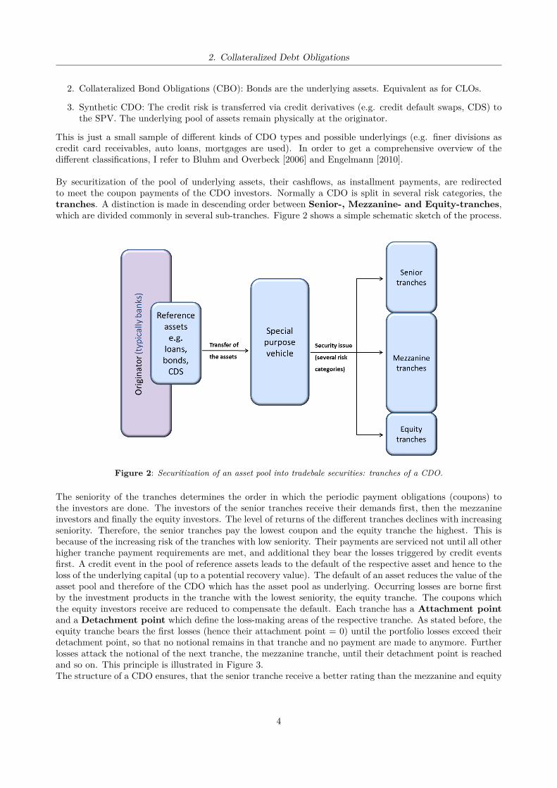
By securitization of the pool of underlying assets, their cashflows, as installment payments, are redirectedto meet the coupon payments of the CDO investors. Normally a CDO is split in several risk categories, thetranches. A distinction is made in descending order between Senior-, Mezzanine- and Equity-tranches,which are divided commonly in several sub-tranches. Figure 2 shows a simple schematic sketch of the process.

Figure 2: Securitization of an asset pool into tradebale securities: tranches of a CDO.

The seniority of the tranches determines the order in which the periodic payment obligations (coupons) tothe investors are done. The investors of the senior tranches receive their demands first, then the mezzanineinvestors and finally the equity investors. The level of returns of the different tranches declines with increasingseniority. Therefore, the senior tranches pay the lowest coupon and the equity tranche the highest. This isbecause of the increasing risk of the tranches with low seniority. Their payments are serviced not until all otherhigher tranche payment requirements are met, and additional they bear the losses triggered by credit eventsfirst. A credit event in the pool of reference assets leads to the default of the respective asset and hence to theloss of the underlying capital (up to a potential recovery value). The default of an asset reduces the value of theasset pool and therefore of the CDO which has the asset pool as underlying. Occurring losses are borne firstby the investment products in the tranche with the lowest seniority, the equity tranche. The coupons whichthe equity investors receive are reduced to compensate the default. Each tranche has a Attachment pointand a Detachment point which define the loss-making areas of the respective tranche. As stated before, theequity tranche bears the first losses (hence their attachment point = 0) until the portfolio losses exceed theirdetachment point, so that no notional remains in that tranche and no payment are made to anymore. Furtherlosses attack the notional of the next tranche, the mezzanine tranche, until their detachment point is reachedand so on. This principle is illustrated in Figure 3.The structure of a CDO ensures, that the senior tranche receive a better rating than the mezzanine and equity

4

3. Introduction of the copula theory and the Gaussian copula model

Figure 3: Allocation of losses and coupon payment waterfall in a CDO contract.

tranches, usually even AAA. Because it bears significantly lower credit risk than the other tranches. Thisalso allows institutional investors, which are legally bounded to best-rated assets, to invest in CDO tranches,although the underlying pool of assets consist of BBB or even worse rated titles.

For the valuation of the CDO tranches you have to model the expected defaults in the underlying asset pool,because as pointed out above, each default has an impact on the CDO payments. In particular, the defaultcorrelation between the different assets is very important for the estimation of fair tranche prices.In practice, there are two basic approaches for pricing CDO tranches:

1. Bottom-up models: The default of every single underlying asset is modeled at lowest level underconsideration of a determined dependence structure between the single assets. By aggregation of thesingle defaults, the simulated tranche loss distribution is estimated.

2. Top-down models: These approaches consider the asset pool as a whole. The cumulative portfolioloss is modeled by a counting process with a determined portfolio intensity. An observation of the singleunderlying assets is not under consideration.

A well-known static bottom-up model is the already mentioned Gaussian copula based approach, presentedby Li [2000]. The next section provides an introduction in the copula theory and then focuses on Li’s modeland it’s flaws, which became apparent clearly during the financial crisis.

3. Introduction of the copula theory and the Gaussian copula modelA copula is a multivariate probability distribution function with uniform marginal distribution functions.Copulas allow to separate the problem of estimating a multidimensional distribution of several variables intothe estimation of the individual marginal distributions and the joint dependency structure between these one-dimensional random variables. This is a major simplification for the pricing of multi-name credit derivatives,like CDOs, where one is mainly interested in the default dependence between different assets. The formaldefinition of a copula is the following one.

Definition 3.1. Let U1, . . . , Un uniformly distributed random variables in [0, 1]. A multivariate distributionfunction Cρ : [0, 1]n → [0, 1] with

Cρ(u1, u2, . . . , un) = P[U1 ≤ u1, U2 ≤ u2, . . . , Un ≤ un]

is called Copula-function, provided that the following conditions are met:

5

3. Introduction of the copula theory and the Gaussian copula model

1. Cρ(u1, u2, . . . , un) = 0, if ui = 0 for at least one i ∈ {1, 2, . . . , n}.

2. Cρ(1, . . . , 1, uk, 1, . . . , 1) = uk for k = 1, . . . , n.

3. Cρ is n-non-decreasing. This means, it is valid for each hyperrectangle∏ni=1[xi, yi] ⊆ [0, 1]n that:∑

(z1,...,zn)∈∏ni=1[xi,yi]

(−1)N(z1,...,zn) · Cρ(z1, . . . , zn) ≥ 0

with N(z1, . . . , zn) := |{k |zk = xk }|.

Here ρ is a general dependence parameter, which characterizes the correlation structure of the copula.

For a copula Cρ : [0, 1]n → [0, 1] and n marginal distribution functions F1(x1), . . . , Fn(xn) of random variablesX1, . . . , Xn it can be concluded that

Cρ(F1(x1), . . . , Fn(xn)) = P[U1 ≤ F1(x1), . . . , Un ≤ Fn(xn)]= P[F−1

1 (U1) ≤ x1, . . . , F−1n (Un) ≤ xn]

= P[X1 ≤ x1, . . . , Xn ≤ xn]= F (x1, . . . , xn)

Then F (x1, . . . , xn) is a copula-dependent multivariate distribution function with associated marginal distri-bution functions F1(x1), . . . , Fn(xn).1 For the marginal distribution functions of the Xi you get:

Cρ(F1(∞), . . . , Fi−1(∞), Fi(xi), Fi+1(∞), . . . , Fn(∞))= P[X1 ≤ ∞, . . . , Xi−1 ≤ ∞, Xi ≤ xi, Xi+1 ≤ ∞, . . . , Xn ≤ ∞]= P[Xi ≤ xi]= Fi(xi)

The following theorem by Sklar is a very important result of the copula theory. It is the reversal of the juststated conclusion and enables the splitting of a multivariate distribution into their marginal distributions andan associated copula function.

Theorem 3.1 (Sklar). Let F be a multivariate n-dimensional distribution function and F1, . . . , Fn the relatedmarginal distribution functions. Then there exists a n-dimensional copula Cρ, so that the following equationholds for all (x1, . . . , xn) ∈ Rn:

F (x1, . . . , xn) = Cρ(F1(x1), . . . , Fn(xn)

).

If all marginal distribution functions F1, . . . , Fn are continuous, then the copula function Cρ is unique, asstated e.g. in O’Kane [2008] or Bluhm and Overbeck [2006]. For a proof of the theorem I refer to Nelsen[2007].It should be emphasized, that Sklar’s theorem "only" ensures the existence of a copula, but the appropriatechoice of a copula function which matches the specific model requirements is fraught with risk. There are avariety of copula functions used in practice which can model different dependence structures. At times of thefinancial crisis the Gaussian copula function was widely used in pricing multi-name credit derivatives dueto Li’s model approach, which became market standard quickly in those days.

Definition 3.2. Let Φ be the distribution function of the one-dimensional standard normal distributionand ΦnΣ the distribution function of the n-dimensional standard normal distribution with positive definitecorrelation matrix Σ. Then the n-dimensional Gaussian copula CΦ

Σ is defined as follows:

CΦΣ (u1, . . . , un) = ΦnΣ

(Φ−1(u1), . . . ,Φ−1(un)

)1Cf. Li [2000]

6

3. Introduction of the copula theory and the Gaussian copula model

for all (u1, . . . , un) ∈ [0, 1]n. For n = 2 you get:

CΦρ12

(u1, u2) =∫ Φ−1(u1)

−∞

∫ Φ−1(u2)

−∞

12π(1− ρ2

12)1/2 exp(−s

2 − 2ρ12 · s · t+ t2

2(1− ρ212)

)dsdt,

with (u1, u2) ∈ [0, 1]2 and ρ12 states for the correlation coefficient of the bivariate standard normal distribution.

The Gaussian copula approach for CDO tranche modeling uses the copula function, introduced in Definition3.2, to incorporate default correlation in the underlying asset pool.Let τi be a random variable, describing the default time of the i-th asset in the underlying pool and F (t1) =P[τ1 ≤ t1] the marginal default time distribution function for i = 1, . . . ,M and M is the number of assetsin the pool. To model the joint default times of all assets in the underlying pool F (t1, . . . , tM ) = P[τ1 ≤t1, . . . , τM ≤ tM ] for all (t1, . . . , tM ) ∈ RM+ you can make use of Sklar’s theorem, which ensures the existenceof a copula C : [0, 1]M → [0, 1], such that

F (t1, . . . , tM ) = C (F1(t1), . . . , FM (tM )) . (1)

Li used in his publication a Gaussian copula C =: CΦΣ . The most common used version of Li’s model is theOne-

factor Gaussian copula model, which offers a high analytical tractability by assuming that the portfolio ofunderlying assets is homogeneous (therefore the model is named "Homogeneous Large Pool Gaussian Copulamodel"). Each asset in the underlying portfolio belongs to a company i with asset value Xi for i = 1, . . . ,M .In the one-factor framework, the value of company i is modeled as

Xi = √ρY +√

1− ρZi, for i = 1, . . . ,M,

where Y,Z1, . . . , ZM are i.i.d. N (0, 1) and ρ ∈ (0, 1). Y is a systematic risk factor, which describes a kind ofmarket risk, common to all companies and the {Zi}Mi=1 present idiosyncratic risk factors, which are specificfor each company i. One of the core assumptions of this model is the flat correlation between each pair ofcompanies due to the homogeneity of the asset pool. This leads to one value ρ for the correlation of every pairof assets.Put it all together, the transpose of the value vector (X1, . . . , XM ) has a multivariate normal distribution:

X1...

XM

∼ NM

000...0

,

1 ρ ρ . . . ρρ 1 ρ . . . ρρ ρ 1 . . . ρ...

......

. . ....

ρ ρ ρ . . . 1

.

A company i defaults if their asset value Xi falls below a threshold. For linking the single default time τi tothe one-factor model, the following relation is used

Xi = Φ−1(Fi(τi))(⇔ τi = F−1

i (Φ(Xi))).

After the marginal distribution functions {Fi}Mi=1 for the {τi}Mi=1 are determined, you can use equation (1)with a Gaussian copula CΦ

Σ to estimate the joint default distribution of the asset pool and after that, Li’sone-factor model is fully specified.In practice the marginal defaults are often modeled as the first jump time of a Poisson process with anintensity rate λi(t), which describes the instantaneous default probability of the company i at time t, and withexponentially distributed jumps

Fi(t) = P[τi ≤ t] = 1− exp{−∫ t

t0

λi(u)du}, t ≥ t0.

Often it is assumed that every individual company has a time constant intensity function λi(t) = λi, whichleads to the default distribution Fi(t) = 1 − exp {−λi · (t− t0)}. These exponential marginals distributionfunctions, together with the market observed prices for the CDO tranches (=̂ market spreads) can be used to

7

4. Limitations and drawbacks of the Gaussian copula in the context of the Financial Crisis

estimate the implied asset correlation ρ for each single tranche. The parameter ρ is calculated so that themarket price matches to the one-factor model. Normally, the value for ρ should be equal for each tranche, butit turns out, that this is unfortunately not the case, which is one important drawback of Li’s model as statedin the next section. For a more comprehensive overview of Li’s model and other copula models I refer to Li[2000], Choros-Tomczyk et al. [2012] and Brigo et al. [2010b].

4. Limitations and drawbacks of the Gaussian copula in the context ofthe Financial Crisis

As already indicated previously, the Gaussian copula model suffers from two main problems, firstly the in-consistencies in implied CDO tranche correlation estimation and secondly the failure in modeling extremalevents due to the missing tail dependence. Obviously, there are still other shortcomings (e.g. see Donnellyand Embrechts [2010] or Brigo et al. [2010a]), but the two mentioned problems are the most striking ones.

Inconsistencies in implied correlations estimation:The implied correlations for each CDO tranche are calculated in such a way that their observed marketspread agree with the used pricing model, in this case with one-factor Gaussian copula model. There are twoapproaches which are widely used in the practice, the compound correlation and the base correlationmethod. The compound correlation approach is similar to the concept of implied volatility. Each tranche isconsidered separately and is priced using a single correlation parameter as input. The parameter is calculatedout of a market spread by inverting the pricing model. By an iteration process you receive the compoundcorrelations of all tranches, which produces a spread that matches the market quote. The presented one-factorGaussian model uses only one correlation ρ for all tranches to specify the loss distribution and the price,so you should get equal correlation values for each tranche by the compound correlation approach. That is,however, precisely the problem, because this method does not produce a unique solution for all tranches, sincethe compound correlation is a function of both, the tranche attachment and detachment point (cf. Lehnertet al. [2005] and Torresetti et al. [2006]). An example of the typical resulting correlation "smile" is illustratedin Figure 4 on the left hand side.

Figure 4: Left graphic: Compound correlations of DJ iTraxx Europe 5-year tranches as of 2004/02/19.Right graphic: DJ iTraxx Europe 5-year 3-6% Tranche spread in bp (y axis), Input Correlation (x axis), asof 2004/02/16. It can be seen that for the traded spread of 227bp, there are two possible correlations. Sourcefor both: JPMorgan.

Additional, many empirical evidence shows that the mezzanine tranches are not monotonic in correlation. Inconsequence, the estimation of the correlation parameter can provide two different results that lead to thesame market spread. Moreover, sometimes the compound correlation parameter can’t be calibrated to themarket data, in these cases it does simply not exist as presented in Figure 4 on the right hand side.

The main idea behind the concept of the base correlation is that every tranche can be decomposed into twofirst loss tranches, which means that you only have to value tranches with lower attachment point zero. For

8

4. Limitations and drawbacks of the Gaussian copula in the context of the Financial Crisis

example, to replicate a long position in a tranche with the attachment points ai and detachment point di youcan take simultaneously a long position in a first-loss-tranche with detachment point di and a short positionin a first-loss-tranche with detachment point ai. By using a bootstrapping technique, you can estimate allbase correlations successively. The concept of base correlations overcomes some limitations of the compoundcorrelations, e.g. it provides a unique implied correlation for fixed attachment points and a wider range oftranche spreads can be inverted into a base correlation value. Additional the approach makes it possible toprice tranches with arbitrary attachment and detachment points which are not traded actively by linearlyinterpolation of the traded tranches.But base correlations also have some drawbacks. The problem of different correlation parameters for eachtranche remains as well as there could be still situations where you can’t calibrate the correlation to themarket spread. Furthermore an new problem arises, the expected tranche loss might become negative undersome market conditions, which violates the basic no-arbitrage constraints. Figure 5 illustrates the appealeddrawbacks.

Figure 5: Left graphic: Base correlations of DJ iTraxx Europe 5-year tranches as of 2004/02/19. Source: JPMorgan.Right graphic: Expected tranche loss as a function of time derived from the base correlations calibrated tothe DJ iTraxx Series 5 10-year tranche spreads as of 2005/08/03. Source Brigo et al. [2010b].

The described inconsistencies of both correlation approaches lead to big problems in the modeling of fairtranche prices and can cause high losses if you apply delta-hedging strategies based on the tranche valuations.Examples on that and further surveys can be found in Torresetti et al. [2006], Brigo et al. [2010a] and Lehnertet al. [2005].

The lack of tail dependence:The Gaussian copula approach can’t model tail dependence. Therefore, the occurrence of extreme events inthe upper and lower tails of the joint distribution of several random variables is dramatically underestimated.This has a big impact on the valuation of CDOs, because the simultaneous default of a large number of assetsin the underlying portfolio can’t be considered in the model. Especially in times of crisis, this might causedangerous inaccurate appraisals of structured products, like CDO tranches.In the following I focus for illustration purposes on the bivariate case and start with a definition.

Definition 4.1. Let (X,Y ) be a bivariate random vector and X and Y two continuous random variables withassociated distribution functions FX and FY .The random variables X and Y are upper tail dependent, if

λU := limu↗1

P[Y > F−1Y (u) | X > F−1

X (u)]

exists and λU ∈ (0, 1]. X and Y are independent in the upper tail if λU = 0.The random variables X and Y are lower tail dependent, if

λL := limu↘0

P[Y ≤ F−1Y (u) | X ≤ F−1

X (u)]

9

4. Limitations and drawbacks of the Gaussian copula in the context of the Financial Crisis

exists and λL ∈ (0, 1]. X and Y are independent in the lower tail if λL = 0.2

The next theorem is stated in Embrechts et al. [2003] and connects tail dependence with the copula approach.

Theorem 4.1. Let X, Y and FX , FY be as introduced in Definition 4.1 and U = FX(X), V = FY (Y ).Therefore U, V ∼ U [0, 1]. Let C be a bivariate copula, which models the joint distribution of X and Y .

1. If λU and λL exist as defined in Definition 4.1, they can be described as follows by application of thecopula C:

λU = limu↗1

1− 2u+ C(u, u)1− u

andλL = lim

u↘0

C(u, u)u

The copula C models upper resp. lower tail dependence, if λU ∈ (0, 1] resp. λL ∈ (0, 1]. C has noupper resp. lower tail dependence, if λU = 0 resp. λL = 0.

2. In addition, if we assume that C has symmetrical arguments, this means C(u, v) = C(v, u) ∀u, v ∈ [0, 1],then we get:

λU = limu↗1

2 · P[V > u | U = u]

andλL = lim

u↘02 · P[V < u | U = u]

A proof of Theorem 4.1 can be found in the appendix A.1.

Theorem 4.1 can be used to show that the Gaussian copula approach fails to model tail dependence. AgainI focus on the bivariate case. Let τ1 and τ2 be the default time variables of two companies with associatedone-dimensional distribution functions F1 and F2. The multivariate distribution function of (τ1, τ2) is modeledwith a Gaussian copula CΦ

ρ12, with estimated correlation coefficient ρ12. Hence:

(τ1, τ2) ∼ CΦρ12

(F1(τ1), F2(τ2)) = Φ2ρ

(Φ−1(F1(τ1)),Φ−1(F2(τ2))

)with ρ12 = ρ.The family of Gaussian copulas is symmetrical in it’s arguments. Therefore, the second statement fromTheorem 4.1 can be applied:

λU = limu↗1

P[τ2 > F−12 (u) | τ1 > F−1

1 (u)]

= 2 · limu↗1

P[F2(τ2) > u | F1(τ1) = u]

The distribution function Φ of the standard-normal distribution does not have a boundary point in the positiverange (R+), so you can express the limit value as follows:

2 · limu↗1

P[F2(τ2) > u | F1(τ1) = u] = 2 · limx→∞

P[Φ−1[F2(τ2)] > x | Φ−1[F1(τ1)] = x]

= 2 · limx→∞

P[X > x | Y = x] (2)

with X = Φ−1[F2(τ2)], Y = Φ−1[F1(τ1)] ∼ N (0, 1) and correlation parameter ρ of (X,Y ).In the bivariate standard-normal case, you get for the conditional distribution:

X|Y = x ∼ N (ρx, 1− ρ2)

2Cf. Nelsen [2007]

10

5. Alternative to the Gaussian copula - mixture of two copulas

This result and the transformation of a normally distributed random variables to a standard-normal randomvariable3 applied to equation (2) leads to:

2 · limx→∞

P[X > x | Y = x] = 2 · limx→∞

[1− Φ

(x− ρx√

1− ρ2

)]

= 2 · limx→∞

[1− Φ

(x ·

√(1− ρ)2

(1− ρ) · (1 + ρ)

)]

= 2 · limx→∞

[1− Φ

(x ·√

1− ρ√1 + ρ

)]= 0 = λU for ρ ∈ (−1, 1)

Equivalent calculation steps result in λL = 0 for ρ ∈ (−1, 1). Alternative, you can use the fact, that theGaussian copula is radially symmetrical.4 From this we have λU = λL.Thus, the Gaussian copula is asymptotically independent in both tails for ρ ∈ (−1, 1).

5. Alternative to the Gaussian copula - mixture of two copulasAs presented in the previous section 4, the Gaussian copula can’t be used to model tail dependence in jointdistribution functions, which is a major weakness (amongst other flaws) of this approach as it turned outduring the Financial Crisis. In order to remedy this problem, at least in part, the choice of another copula tomodel the joint defaults of assets in an underlying pool for a CDO, may be more suitable. In financial marketsit could be expected that large joint losses of several companies, resp. assets occur more often than large jointgains, at least if you rely on more conservative valuation approaches. Especially in times of crisis, this is nobad assumption. Therefore a way to model asymmetric tail dependence is required, which leads to the class ofArchimedean copulas. Two representatives of this class are the Gumbel and the Clayton copula, whichare both asymmetric copulas, that are able to model upper and lower tail dependence, but each only in onedirection. However, it is possible to create a mixture of both, which is still a copula function and has theproperty of asymmetric tail dependence. Before this point is considered in more detail I refer to the book ofNelsen [2007] to get an introduction of the theory of Archimedean copulas.

Theorem 5.1. Let C1ρ1

and C2ρ2

two copula functions and θ ∈ [0, 1]. A linear convex combination Cρ of C1ρ1

and C2ρ2

is still a copula function:

C12ρ1,ρ2

(u1, u2, . . . , un; θ) = θC1ρ1

(u1, u2, . . . , un) + (1− θ)C2ρ2

(u1, u2, . . . , un).

A proof of this can be found in Nelsen [2007]. For a mixture of a Clayton CCρC and a Gumbel CGρG copula inthe bivariate case you get

CCGρC ,ρG(u1, u2; θ) = θCCρC (u1, u2) + (1− θ)CGρG(u1, u2)

withCCρC (u1, u2) = (u−ρC1 + u−ρC2 − 1)−ρ

−1C , ∀ρC > 0

andCGρG(u1, u2) = exp

(− [(− log u1)ρG + (− log u2)ρG ]

1ρG

), ∀ρG ∈ [−1,∞).

If viewed separately, the following values for the tail dependence parameters can be estimated for the Claytonand Gumbel copula, as stated in the appendix A.2:

1. Clayton copula: λU = 0 and λL = 2−1ρC

3It holds that: W ∼ N (µ, σ2) =⇒ W−µσ∼ N (0, 1)

4Cf. McNeil et al. [2005], "radial symmetric" means: Let (U1, . . . , Un) ∼ C with appropriate copula C. C is called radialsymmetric if: (U1 − 0.5, . . . , Un − 0.5) d= (0.5− U1, . . . , 0.5− Un)⇔ U d= 1−U with 1,U ∈ R1×n

11

6. Conclusion

2. Gumbel copual: λU = 2− 21ρG and λL = 0.

This means that a Clayton copula can be used to model lower tail dependence and a Gumbel copula is ableto model upper tail dependence, by appropriate selection of ρC and ρG. Therefore, a mixture of both canbe used to model asymmetric tail dependence for the upper and lower tail. The parameters λ12

U and λ12L for

a combination of two copulas can easily be estimated, if you know the tail dependence parameters of everysingle copula λ1

U , λ2U and λ1

L, λ2L and if you have defined the weight coefficient θ ∈ [0, 1]:

λ12U = θλ1

U + (1− θ)λ2U and

λ12L = θλ1

L + (1− θ)λ2L.

The parameter θ should be estimated by market calibration under consideration of extreme events, such as thesimultaneous default of many companies as observed during the Financial Crisis. By the mixture of two copulasyou gain much flexibility in modeling dependence structures compared to the Gaussian copula approach andthis might be one possibility to overcome one of the most serious flaws of this approach.

6. ConclusionThe exploding popularity, beginning in the early 2000’s, of the securitization of loan receivables by financialinstitutions and especially the pricing of the resulting multi-name credit derivatives by copula approachescan be illustrated with a simple example: While a Google search for the word "copula" yields about 10,000hits in the year 2003 as stated in Mikosch [2006], the same search results in approximately 1,3 million hits inthe year 2007 as written by the Financial Times.The Gaussian copula approach presented in Li [2000], provides a fast and very practicable opportunity to pricethe highly complex multi-name credit derivatives, mostly CDOs, using only a few market observable parame-ters. In addition to the simplicity of the valuation approach, the financial institutions obtained very lucrativeprofits by issuing CDOs and as a side effect, they got rid of huge parts of their credit risks. Consequently itwas not surprising that the market for these products grew ever more rapidly and that early warning signalswere ignored.The limitations of the Gaussian copula approach, discussed in Section 4 and further drawbacks were alreadywell known and published before the Financial Crisis. However, there were a large number of more or lesspopulist articles, like "The formula that felled Wall St" (Financial Times), "Wall Street’s Math Wizards forgota few variables" (New York Times) or "Recipe for disaster: the Formula that killed Wall Street" (Wired mag-azine) which blamed the academics and mathematicians to be responsible for the Financial Crisis. In theirreadable work Brigo et al. [2010a] rejected this critique and clarified that in particular academics had warnedbefore the crisis to rely blindly on the Gaussian copula approach.In order to make it perfectly clear, a mathematical model alone, cannot be responsible for the Financial Crisisand its consequences. All involved parties, namely risk managers and financial institutions must be aware ofthe flaws and risks of the models they apply. They are responsible to choose appropriate models for the ap-plications under consideration and they need to know what are the structures and properties of these models.The question remains if there is a "right" copula, which should have been used to prevent the crisis? Themixture of two copulas, e.g. a Clayton and Gumbel copula, as introduced in Section 5 can overcome someof the drawbacks of the Gaussian copula approach, but others still remain and maybe new problems arise.Hence, as stated before, it should be borne in mind that you are always dealing "only" with a mathematicalmodel and a model is not able to fully capture all factors having an effect in reality - therefore do not blindlytrust to it. Only if this is clear to the people and they generally act accordingly, the next Financial Crisis canbe prevented.

ReferencesChristian Bluhm and Ludger Overbeck. Structured Credit Portfolio Analysis, Baskets and CDOs. Crc Pr Inc,1 edition, October 2006. ISBN 1584886471.

12

A. Mathematical appendix

Damiano Brigo, Andrea Pallavicini, and Roberto Torresetti. Credit models and the crisis, or: how I learnedto stop worrying and love the CDOs. February 2010a. URL http://arxiv.org/abs/0912.5427.

Damiano Brigo, Andrea Pallavicini, and Roberto Torresetti. Credit Models and the Crisis: A Journey intoCDOs, Copulas, Correlations and Dynamic Models. John Wiley & Sons, 1. edition edition, 2010b.

Barbara Choros-Tomczyk, Wolfgang Karl Härdle, and Ludger Overbeck. Copula dynamics in cdos. SFB649 Discussion Papers SFB649DP2012-032, Humboldt University, Collaborative Research Center 649, 2012.URL http://EconPapers.repec.org/RePEc:hum:wpaper:sfb649dp2012-032.

Catherine Donnelly and Paul Embrechts. The devil is in the tails: Actuarial mathematics and the subprimemortgage crisis. ASTIN Bulletin: The Journal of the International Actuarial Association, 40(01):1–33, 2010.URL http://EconPapers.repec.org/RePEc:cup:astinb:v:40:y:2010:i:01:p:1-3300.

Paul Embrechts, Filip Lindskog, and Alexander McNeil. Modelling dependence with copulas and applicationsto risk management. In Svetlozar T. Rachev, editor, Handbook of Heavy Tailed Distributions in Finance,chapter 8, pages 329 – 384. Elsevier, 2003.

Susann Engelmann. Collateralized debt obligation and its impact to the financial crisis. Hans-Böckler-StiftungeLibrary, 2010.

Erik Forslund and Daniel Johansson. Gaussian copula what happens when models fail? 2012.

Nicole Lehnert, Frank Altrock, Svetlozar T. Rachev, Stefan Trück, and Andre Wilch. Implied correlations incdo tranches. 2005.

David X. Li. On Default Correlation: A Copula Function Approach. Journal of Fixed Income, 9(4):43–54,March 2000. URL http://www.defaultrisk.com/pp_corr_05.htm.

Alexander J. McNeil, Rüdiger Frey, and Paul Embrechts. Quantitative Risk Management: Concepts, Tech-niques and Tools. Princeton University Press, 2005.

Thomas Mikosch. Copulas: Tales and facts. Extremes, 9(1):3–20, 2006.

Roger B. Nelsen. An Introduction to Copulas. Springer New York, 2. edition, corrected second printing edition,2007.

Dominic O’Kane. Modelling Single-name and Multi-name Credit Derivatives (Wiley Finance). John Wiley &Sons, 1. auflage edition, 7 2008. ISBN 9780470519288.

Roberto Torresetti, Damiano Brigo, and Andrea Pallavicini. Implied correlation in cdo tranches: A paradigmto be handled with care. Available at SSRN 946755, 2006.

A. Mathematical appendixA.1. Proof of Theorem 4.1The proof is based on the sketch presented in Embrechts et al. [2003].

Proof. The proof is only executed for λU . However, the assertions for λL follow equivalently.

1. The first assertion: For λU and a bivariate copula C with (X,Y ) ∼ C(FX(X), FY (Y )) the following isvalid:

λU = limu↗1

P[Y > F−1Y (u) | X > F−1

X (u)]

= limu↗1

P[FY (Y ) > u | FX(X) > u]

13

A. Mathematical appendix

= limu↗1

P[FY (Y ) > u,FX(X) > u]P[FX(X) > u]

= limu↗1

1− (P[FX(X) ≤ u] + P[FY (Y ) ≤ u]− P[FX(X) ≤ u, FY (Y ) ≤ u])1− P[FX(X) ≤ u]

= limu↗1

1− 2u+ C(u, u)1− u ,because of FX(X), FY (Y ) ∼ U [0, 1] (3)

2. The second assertion: The numerator and denominator of equation (3) converge towards 0 for u→ 1, soyou can use L’Hôpital’s rule:

limu↗1

1− 2u+ C(u, u) = 1− 2 + 1 = 0 and

limu↗1

1− u = 1− 1 = 0

It follows

limu↗1

1− 2u+ C(u, u)1− u = lim

u↗1

[−2 + dC(u,u)

du−1

]

= − limu↗1

[−2 + ∂

∂sC(s, t)

∣∣∣s=t=u

+ ∂

∂tC(s, t)

∣∣∣s=t=u

]. (4)

In the next step I introduce an interim result which is needed in the following:

P[V ≤ v | U = u] = lim∆u→0

P[V ≤ v | u ≤ U ≤ u+ ∆u]

= lim∆u→0

P[V ≤ v, u ≤ U ≤ u+ ∆u]P[u ≤ U ≤ u+ ∆u]

= lim∆u→0

P[V ≤ v, U ≤ u+ ∆u]− P[V ≤ v, U ≤ u]P[U ≤ u+ ∆u]− P[U ≤ u]

= lim∆u→0

C(u+ ∆u, v)− C(u, v)∆u

= ∂

∂uC(u, v)

Hence, you getP[V > v | U = u] = 1− ∂

∂uC(u, v)

andP[U > u | V = v] = 1− ∂

∂vC(u, v).

From this result and equation (4), you can deduce the second assertion:

λU = − limu↗1

[−2 + ∂

∂sC(s, t)

∣∣∣s=t=u

+ ∂

∂tC(s, t)

∣∣∣s=t=u

]= limu↗1

[1− ∂

∂sC(s, t)

∣∣∣s=t=u

+ 1− ∂

∂tC(s, t)

∣∣∣s=t=u

]= limu↗1

P[V > u | U = u] + P[U > u | V = u]

= 2 · limu↗1

P[V > u | U = u] (5)

14

A. Mathematical appendix

A.2. Tail dependence of bivariate Gumbel and Clayton copula’sFor a bivariate Gumbel copula it holds:

CGρG(u, u) = exp(− [(− log u)ρG + (− log u)ρG ]

1ρG

)= exp

(− [−2(log u)ρG ]

1ρG

)= exp

(2

1ρG log u

)= u2

1ρG .

The use of Theorem 4.1 finally leads to the parameter for the upper and lower tail dependence coefficient.Upper tail dependence coefficient for a bivariate Gumbel copula:

λU = limu↗1

1− 2u+ CGρG(u, u)1− u

= limu↗1

1− 2u+ u21ρG

1− u (6)

The numerator and denominator of equation (6) converge towards 0 for u → 1, so you can use L’Hôpital’srule:

= limu↗1

−2 + 21ρG u2

1ρG −1

−1= 2− 2

1ρG

Lower tail dependence coefficient for a bivariate Gumbel copula:

λL = limu↘0

CGρG(u, u)u

= limu↘0

u21ρG

u

Again with L’Hôpital’s rule it follows:

= limu↘0

21ρG u2

1ρG −1

1= 0

Equivalently, you get for a bivariate Clayton copula:

CCρC (u, u) = (u−ρC + u−ρC − 1)−ρ−1C

= (2u−ρC − 1)−ρ−1C .

Consequently you can deduce the upper and lower tail dependence coefficient by usage of Theorem 4.1 andL’Hôpital’s rule.

15

A. Mathematical appendix

Upper tail dependence coefficient for a bivariate Clayton copula:

λU = limu↗1

1− 2u+ CCρC (u, u)1− u

= limu↗1

1− 2u+ (2u−ρC − 1)−ρ−1C

1− u

= limu↗1

−2 + 2u−ρC−1(2u−ρC − 1)−ρ−1C −1

−1= 0

Lower tail dependence coefficient for a bivariate Clayton copula:

λL = limu↘0

CCρC (u, u)u

= limu↘0

(2u−ρC − 1)−ρ−1C

u

= limu↘0

(2u−ρC − 1)−ρ−1C

(uρC )ρ−1C

= limu↘0

(2− uρC )−ρ−1C

= 2−1ρC

A.3. Tail dependence and mixtures of two copula’sFor the upper tail dependence of a mixture copula C12, consisting of a convex combination of two copula’s C1

and C2, it can be deduced

λ12U = lim

u↗1

1− 2u+ C12(u, u)1− u

= limu↗1

1− 2u+ θC1(u, u) + (1− θ)C2(u, u)1− u

= limu↗1

θ(1− 2u+ C1(u, u)) + (1− θ)(1− 2u+ C2(u, u))1− u

= θ limu↗1

1− 2u+ C1(u, u)1− u + (1− θ) lim

u↗1

1− 2u+ C2(u, u)1− u

= θλ1U + (1− θ)λ2

U .

Analogously you can estimate the lower tail dependence of C12:

λ12L = lim

u↘0

C12(u, u)u

= limu↘0

θC1(u, u) + (1− θ)C2(u, u)u

= θλ1L + (1− θ)λ2

L.

16