Gaussian Process Vine Copulas forMultivariate Dependence

Jose Miguel Hernandez-Lobato1,2

joint work with David Lopez-Paz2,3 and Zoubin Ghahramani1

1Department of Engineering, Cambridge University, Cambridge, UK3Max Planck Institute for Intelligent Systems, Tubingen, Germany

April 29, 2013

2Both authors are equal contributors.1

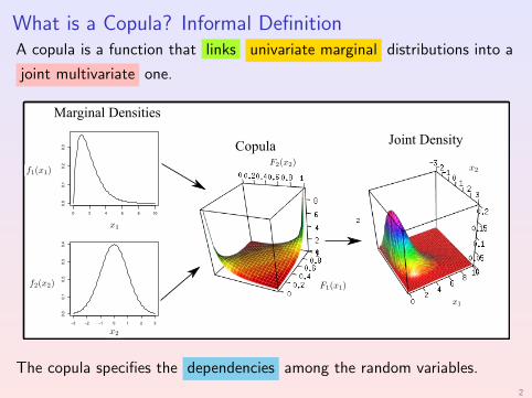
What is a Copula? Informal DefinitionA copula is a function that links univariate marginal distributions into a

joint multivariate one.

−3 −2 −1 0 1 2 3

0.0

0.1

0.2

0.3

0.4

x

0 2 4 6 8 10

0.0

0.1

0.2

0.3

y

Marginal Densities

Copula Joint Density

The copula specifies the dependencies among the random variables.

2

What is a Copula? Formal DefinitionA copula is a distribution function with marginals uniform in [0, 1] .

Let U1, . . . ,Ud be r.v. uniformly distributed in [0, 1] with copula C then

C (u1, . . . , ud) = p(U1 ≤ u1, . . . ,Ud ≤ ud) .

Sklar’s theorem (connection between joints, marginals and copulas)

Any joint cdf F (x1, . . . , xd) with marginal cdfs F1(x1), . . . ,Fd(xd) satisfies

F (x1, . . . , xd) = C (F1(x1), . . . ,Fd(xd)) ,

where C is the copula of F .

It is easy to show that the joint pdf f can be written as

f (x1, . . . , xd) = c(F1(x1), . . . ,Fd(xd))d∏

i=1

fi (xi ) ,

c(u1, . . . , ud) and f1(x1), . . . , fd(xd) are the copula and marginal densities.3

Why are Copulas Useful in Machine Learning?

The converse of Sklar’s theorem is also true:

Given a copula C : [0, 1]d → [0, 1] and margins F1(x1), . . . ,Fd(xd) thenC (F1(x1), . . . ,Fd(xd)) represents a valid joint cdf.

Copulas are a powerful tool for the modeling of multivariate data .

We can easily extend univariate models to the multivariate regime.

Copulas simplify the estimation process for multivariate models.

I 1 - Estimate the marginal distributions.I 2 - Map the data to [0, 1]d using the estimated marginals.I 3 - Estimate a copula function given the mapped data.

Learning the marginals : easily done using standard univariate methods.

Learning the copula : difficult, requires to use copula models that i) canrepresent a broad range of dependencies and ii) are robust to overfitting.

4

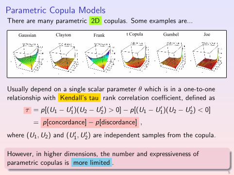
Parametric Copula ModelsThere are many parametric 2D copulas. Some examples are...

Clayton FrankGaussian Gumbel Joet Copula

Usually depend on a single scalar parameter θ which is in a one-to-onerelationship with Kendall’s tau rank correlation coefficient, defined as

τ = p[(U1 − U ′1)(U2 − U ′2) > 0]− p[(U1 − U ′1)(U2 − U ′2) < 0]

= p[concordance]− p[discordance] ,

where (U1,U2) and (U ′1,U′2) are independent samples from the copula.

However, in higher dimensions, the number and expressiveness ofparametric copulas is more limited .

5

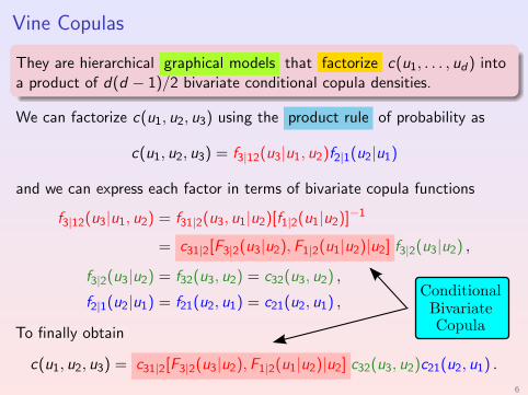
Vine Copulas

They are hierarchical graphical models that factorize c(u1, . . . , ud) intoa product of d(d − 1)/2 bivariate conditional copula densities.

We can factorize c(u1, u2, u3) using the product rule of probability as

c(u1, u2, u3) = f3|12(u3|u1, u2)f2|1(u2|u1)

and we can express each factor in terms of bivariate copula functions

6

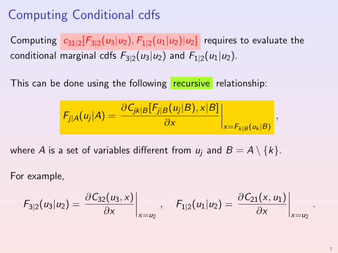
Computing Conditional cdfs

Computing c31|2[F3|2(u3|u2),F1|2(u1|u2)|u2] requires to evaluate the

conditional marginal cdfs F3|2(u3|u2) and F1|2(u1|u2).

This can be done using the following recursive relationship:

Fj |A(uj |A) =∂Cjk|B [Fj |B(uj |B), x |B]

∂x

∣∣∣∣x=Fk|B(uk |B)

,

where A is a set of variables different from uj and B = A \ {k}.

For example,

F3|2(u3|u2) =∂C32(u3, x)

∂x

∣∣∣∣x=u2

, F1|2(u1|u2) =∂C21(x , u1)

∂x

∣∣∣∣x=u2

.

7

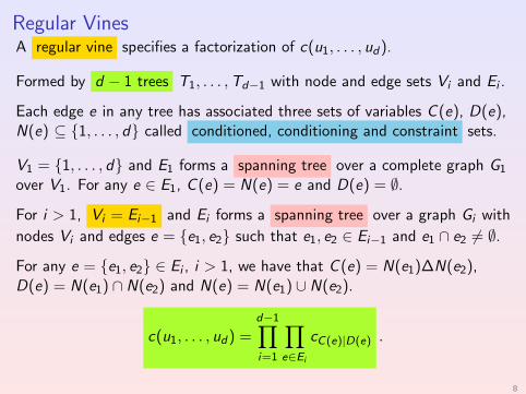
Regular VinesA regular vine specifies a factorization of c(u1, . . . , ud).

Formed by d − 1 trees T1, . . . ,Td−1 with node and edge sets Vi and Ei .

Each edge e in any tree has associated three sets of variables C (e), D(e),N(e) ⊆ {1, . . . , d} called conditioned, conditioning and constraint sets.

V1 = {1, . . . , d} and E1 forms a spanning tree over a complete graph G1

over V1. For any e ∈ E1, C (e) = N(e) = e and D(e) = ∅.

For i > 1, Vi = Ei−1 and Ei forms a spanning tree over a graph Gi with

nodes Vi and edges e = {e1, e2} such that e1, e2 ∈ Ei−1 and e1 ∩ e2 6= ∅.

For any e = {e1, e2} ∈ Ei , i > 1, we have that C (e) = N(e1)∆N(e2),D(e) = N(e1) ∩ N(e2) and N(e) = N(e1) ∪ N(e2).

c(u1, . . . , ud) =d−1∏i=1

∏e∈Ei

cC(e)|D(e) .

8

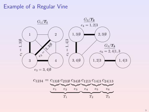
Example of a Regular Vine

9

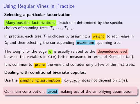
Using Regular Vines in Practice

Selecting a particular factorization:

Many possible factorizations . Each one determined by the specificchoices of spanning trees T1, . . . ,Td−1.

In practice, each tree Ti is chosen by assigning a weight to each edge in

Gi and then selecting the corresponding maximum spanning tree.

The weight for the edge e is usually related to the dependence levelbetween the variables in C (e) (often measured in terms of Kendall’s tau).

It is common to prune the vine and consider only a few of the first trees.

Dealing with conditional bivariate copulas:

Use the simplifying assumption : cC(e)|D(e) does not depend on D(e).

Our main contribution: avoid making use of the simplifying assumption.

10

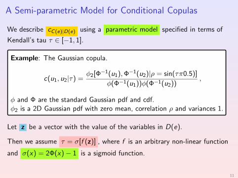
A Semi-parametric Model for Conditional Copulas

We describe cC(e)|D(e) using a parametric model specified in terms of

Kendall’s tau τ ∈ [−1, 1].

Let z be a vector with the value of the variables in D(e).

Then we assume τ = σ[f (z)] , where f is an arbitrary non-linear function

and σ(x) = 2Φ(x)− 1 is a sigmoid function.

11

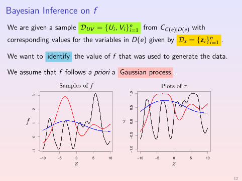
Bayesian Inference on f

We are given a sample DUV = {Ui ,Vi}ni=1 from CC(e)|D(e) with

corresponding values for the variables in D(e) given by Dz = {zi}ni=1 .

We want to identify the value of f that was used to generate the data.

We assume that f follows a priori a Gaussian process .

−10 −5 0 5 10

−10

12

3

−10 −5 0 5 10

−1.0

−0.5

0.0

0.5

1.0

12

Posterior and Predictive Distributions

The posterior distribution for f = (f1, . . . , fn)T, where fi = f (zi ), is

p(f|DUV ,Dz) =[∏n

i=1 c(Ui ,Vi |τ = σ[fi ])] p(f|Dz)

p(DUV |Dz),

where p(f|Dz) = N (f|m0,K) is the Gaussian process prior on f.

Given zn+1, the predictive distribution for Un+1 and Vn+1 is

p(un+1, vn+1|zn+1,DUV ,Dz) =

∫c(un+1, vn+1|τ = σ[fn+1])

p(fn+1|f, zn+1,Dz)p(f|DUV ,Dz)df ,

For efficient approximate inference, we use Expectation Propagation .

13

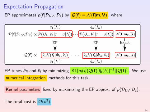
Expectation Propagation

EP approximates p(f|DUV ,Dz) by Q(f) = N (f|m,V) , where

EP tunes mi and vi by minimizing KL[qi (fi )Q(f)[qi (fi )]−1||Q(f)] . We use

numerical integration methods for this task.

Kernel parameters fixed by maximizing the EP approx. of p(DUV |Dz).

The total cost is O(n3) .

14

Implementation Details

We choose the following covariance function for the GP prior:

Cov[f (zi ), f (zj)] = σ exp{−(zi − zj)

Tdiag(λ)(zi − zj)}

+ σ0 .

The mean of the GP prior is constant and equal to Φ−1((τMLE + 1)/2) ,where τMLE is the MLE of τ for an unconditional Gaussian copula.

We use the FITC approximation:

K approximated by K′ = Q + diag(K−Q), where Q = Knn0K−1n0n0K

Tnn0 .

Kn0n0 is the n0 × n0 covariance matrix for n0 � n pseudo-inputs .

Knn0 contains the covariances between training points and pseudo-inputs.

The cost of EP is now O(nn20) . We choose n0 = 20.

The predictive distribution is approximated using sampling .

15

Experiments IWe compare the proposed method GPVINE with two baselines:

1 - SVINE , based on the simplifying assumption.

2 - MLLVINE , based on the maximization of the local likelihood.

Can only capture dependencies on a single random variable.

Limited to regular vines with at most two trees .

All the data mapped to [0, 1]d using the ecdfs.

Synthetic Data: Z uniform in [−6, 6] and (U,V ) Gaussian withcorrelation 3/4 sin(Z ). Data set of size 50.

0.0 0.2 0.4 0.6 0.8 1.0

-0.6

-0.2

0.2

0.6

PZ (Z)

τ U,V

|Z

GPVINEMLLVINETRUE

16

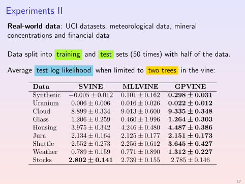
Experiments II

Real-world data: UCI datasets, meteorological data, mineralconcentrations and financial data

Data split into training and test sets (50 times) with half of the data.

Average test log likelihood when limited to two trees in the vine:

17

Results for More than Two Trees

GPVINESVINE

18

Conditional Dependencies in Weather Data

Conditional Kendall’s tau foratmospheric pressure and

cloud percentage coverwhen conditioned to latitudeand longitude near Barcelonaon 11/19/2012 at 8pm.

xxxxxxxxxxxxxx xxxxxxxxxx xx xxxx

xx

xx xx

xx xxxx xxx xx xxxx

xx xxx xxx

xxx xxx xxxxxx

xxxx

xxx xxx

xx

x

xxxxx

x

x

x

x

x xxx

x

xx

xx x

xx x x

x

x

x

xxxx

x

xxxx

xxx

xx

xx xx

x

x

xx

xx xx

x

xxxx

x

x

xx

xx

xx

x

xx

x

xx

xx

xx

x

xx

xx

xx

xx

x xxx

x

xx

xx

x

x

xx x

x

xxx x x

x

xx

x

x

x

xxxxx xxxx

x

xxx xxxx

xx

x

xxxx x

xx

xxx xxx x

x

xxxx

x

x

xxx xxxxx xx xxxx x

xx

xx xx

x

x

x

x

x

x

x

x

x

x

x

x

x

x

x

x

x

x

xx

x

x

x

xx x

x x

xx

xx

x

x

x x

x

x

x

x

x xx

xx

x x

x

xx

x

x

x xx

x

x

x xx

x

x

x

x

x

x

xxx

x x xx

xx

xx

xx

x

x x

x

x

x

x x x

x

xxx xx

x

x

x

xx

x

xx xx

x

x xx x

x

xx

x

x

x

xx

xx

x

x xx

x

x xx

x

x x xxx

xxxxx xx x xx x x xxxx xx

x

x

x

x

xx x

x

x xxxx

x

x

x

x

x xx xx

x

x

x

x

x

x

x x

x

xxx

x

xxx xxx x

x

x

x

x

x

x

x

x

x

x

x

x

x

x xxxxx

x

xx

x

xx

xx

xx x

x

x

x

x

x xxx

x

xx

x

x

x

x

x

x

x

x

xxx

x

x xxx

x

xx

x

x

x

xxx

xx

xxx

x

x

xxx

x

xxx

x

x

x

x

xxx

x

x

x

xxx

xx

x

x

xx x

x

xx

x

x

xx

x xx x

x

xx

x

xx

x

x x

x

x

xx

x

xxxxx

x

x

x xxx

x

x

xx

x

xx

x

x

x

x

x

x

x

x

x x

x

x

x

x xx

x

x

x

xx

x

xx x

x

x

xxx

x

xxx

x

xx

x

xxx

xx

x

x

x

xx

x

xx

x

x

x

xx

xx

x

x

x

x

xx

x

xx

x

x

xx

x

xx

xx

x

x

x

x

x

x

x

x

x

x

x

x

xx

x

x

x

x

x

x

x

xx

x

x

xx

x

x

xx

x

xxx

x

x

x

xx

x

xx

x

x

x

x

x

x

x

xxx

x

xx

xx

xx

xxx

x

xx

x

x

xx

x

x

x

x

x

x x x

x

x

x

x

x

x

x

x

xx

x

x x

x

x

x

xx

x

x

x

x

x

xx

x

xx xx

x

x

x xx

x

x

x

x

x

x

xx xx

x x

x

x

xxx

x

x

x

xx

x

x

xx

x

xx

x

xx

x

x

x

x

x

x

x

x

x

x

xx

x

x

x

x

x

x

x

xx

x

x

x

x

xxxx

xx

x

xx

x

x x

x

x

x

xx

x

xxx

x

x

xx

x

x

x

xx

x

x

x

x

x

x

x

x

xxx

x

x

x

x

x

xx

x

x

x

xx

xx

x

xx

x

xx

x

x

x

x

x

x

x

x

x

x

x

xx

x

x

x

x

x

x

xx

x

x

x

x

xx

x

x

x

x x

x

x

x

xx

xx xx

x

x

xx

19

Summary and Conclusions

Vine copulas are flexible models for multivariate dependencies which

specify a factorization of the copula density into a product of conditionalbivariate copulas.

In practical implementations of vines, some of the conditional

dependencies in the bivariate copulas are usually ignored .

To avoid this, we have proposed a method for the estimation offully conditional vines using Gaussian processes (GPVINE).

GPVINE outperforms a baseline that ignores conditional dependencies(SVINE) and other alternatives based on maximum local-likelihoodmethods (MLLVINE).

20

References

Lopez-Paz D., Hernandez-Lobato J. M. and Ghahramani Z. GaussianProcess Vine Copulas for Multivariate Dependence International Conferenceon Machine Learning (ICML 2013).

Acar, E. F., Craiu, R. V., and Yao, F. Dependence calibration in conditionalcopulas: A nonparametric approach. Biometrics, 67(2):445-453, 2011.

Bedford, T. and Cooke, R. M. Vines-a new graphical model for dependentrandom variables. The Annals of Statistics, 30(4):1031-1068, 2002

Minka, T. P. Expectation Propagation for approximate Bayesian inference.Proceedings of the 17th Conference in Uncertainty in Artificial Intelligence,pp. 362-369, 2001.

Naish-Guzman, A. and Holden, S. B. The generalized FITC approximation.In Advances in Neural Information Processing Systems 20, 2007.

Patton, A. J. Modelling asymmetric exchange rate dependence.International Economic Review, 47(2):527-556, 2006

21

Thank you for your attention!

22