gaussian processes for data-efficient learning in robotics ... · gaussian processes for...
TRANSCRIPT

IEEE TRANSACTIONS ON PATTERN ANALYSIS AND MACHINE INTELLIGENCE, VOL. 37, NO. 2, FEBRUARY 2015 1
Gaussian Processes for Data-Efficient Learningin Robotics and Control
Marc Peter Deisenroth, Dieter Fox, and Carl Edward Rasmussen
Abstract—Autonomous learning has been a promising direction in control and robotics for more than a decade since data-drivenlearning allows to reduce the amount of engineering knowledge, which is otherwise required. However, autonomous reinforcementlearning (RL) approaches typically require many interactions with the system to learn controllers, which is a practical limitation in realsystems, such as robots, where many interactions can be impractical and time consuming. To address this problem, current learningapproaches typically require task-specific knowledge in form of expert demonstrations, realistic simulators, pre-shaped policies, orspecific knowledge about the underlying dynamics. In this article, we follow a different approach and speed up learning by extractingmore information from data. In particular, we learn a probabilistic, non-parametric Gaussian process transition model of the system. Byexplicitly incorporating model uncertainty into long-term planning and controller learning our approach reduces the effects of modelerrors, a key problem in model-based learning. Compared to state-of-the art RL our model-based policy search method achieves anunprecedented speed of learning. We demonstrate its applicability to autonomous learning in real robot and control tasks.
Index Terms—Policy search, robotics, control, Gaussian processes, Bayesian inference, reinforcement learning
F
1 INTRODUCTION
ONE of the main limitations of many current rein-forcement learning (RL) algorithms is that learning is
prohibitively slow, i.e., the required number of interactionswith the environment is impractically high. For example,many RL approaches in problems with low-dimensionalstate spaces and fairly benign dynamics require thousandsof trials to learn. This data inefficiency makes learning inreal control/robotic systems impractical and prohibits RLapproaches in more challenging scenarios.
Increasing the data efficiency in RL requires either task-specific prior knowledge or extraction of more informationfrom available data. In this article, we assume that expertknowledge (e.g., in terms of expert demonstrations [48],realistic simulators, or explicit differential equations for thedynamics) is unavaiable. Instead, we carefully model theobserved dynamics using a general flexible nonparametricapproach.
Generally, model-based methods, i.e., methods whichlearn an explicit dynamics model of the environment, aremore promising to efficiently extract valuable informationfrom available data [5] than model-free methods, such as
• M.P. Deisenroth is with the Department of Computing, Imperial CollegeLondon, 180 Queen’s Gate, London SW7 2AZ, United Kingdom, and withthe Department of Computer Science, TU Darmstadt, Germany.
• D. Fox is with the Department of Computer Science & Engineering,University of Washington, Box 352350, Seattle, WA 98195-2350.
• C.E. Rasmussen is with the Department of Engineering, University ofCambridge, Trumpington Street, Cambridge CB2 1PZ, United Kingdom.
Manuscript received 15 Sept. 2012; revised 6 May 2013; accepted 20 Oct.2013; published online 4 November 2013.Recommended for acceptance by R.P. Adams, E. Fox, E. Sudderth, andY.W. Teh.For information on obtaining reprints of this article, please send e-mail to:[email protected] and reference IEEECS Log NumberTPAMISI-2012-09-0742.Digital Object Identifier no. 10.1109/TPAMI.2013.218
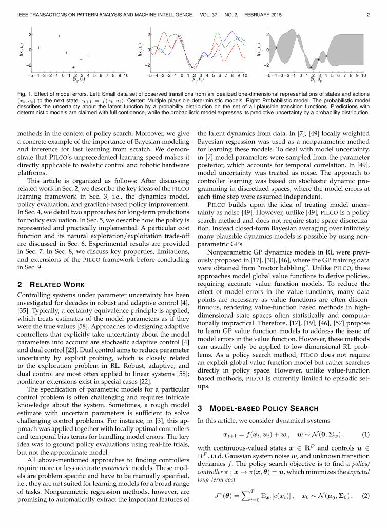
Q-learning [55] or TD-learning [52]. The main reason whymodel-based methods are not widely used in RL is that theycan suffer severely from model errors, i.e., they inherentlyassume that the learned model resembles the real envi-ronment sufficiently accurately [5], [48], [49]. Model errorsare especially an issue when only a few samples and noinformative prior knowledge about the task are available.Fig. 1 illustrates how model errors can affect learning. Givena small data set of observed transitions (left), multipletransition functions plausibly could have generated them(center). Choosing a single deterministic model has severeconsequences: Long-term predictions often leave the rangeof the training data in which case the predictions become es-sentially arbitrary. However, the deterministic model claimsthem with full confidence! By contrast, a probabilistic modelplaces a posterior distribution on plausible transition func-tions (right) and expresses the level of uncertainty about themodel itself.
When learning models, considerable model uncertaintyis present, especially early on in learning. Thus, we requireprobabilistic models to express this uncertainty. Moreover,model uncertainty needs to be incorporated into plan-ning and policy evaluation. Based on these ideas, we pro-pose PILCO (Probabilistic Inference for Learning Control),a model-based policy search method [15], [16]. As a prob-abilistic model we use nonparametric Gaussian processes(GPs) [47]. PILCO uses computationally efficient determin-istic approximate inference for long-term predictions andpolicy evaluation. Policy improvement is based on ana-lytic policy gradients. Due to probabilistic modeling andinference PILCO achieves unprecedented learning efficiencyin continuous state-action domains and, hence, is directlyapplicable to complex mechanical systems, such as robots.
In this article, we provide a detailed overview of the keyingredients of the PILCO learning framework. In particular,we assess the quality of two different approximate inference
arX
iv:1
502.
0286
0v2
[st
at.M
L]
10
Oct
201
7
IEEE TRANSACTIONS ON PATTERN ANALYSIS AND MACHINE INTELLIGENCE, VOL. 37, NO. 2, FEBRUARY 2015 2
−5 −4 −3 −2 −1 0 1 2 3 4 5 6 7 8 9 10
−2
0
2
(xt, u
t)
f(x
t, u
t)
−5 −4 −3 −2 −1 0 1 2 3 4 5 6 7 8 9 10
−2
0
2
(xt, u
t)
f(x
t, u
t)
−5 −4 −3 −2 −1 0 1 2 3 4 5 6 7 8 9 10
−2
0
2
(xt, u
t)
f(x
t, u
t)
Fig. 1. Effect of model errors. Left: Small data set of observed transitions from an idealized one-dimensional representations of states and actions(xt, ut) to the next state xt+1 = f(xt, ut). Center: Multiple plausible deterministic models. Right: Probabilistic model. The probabilistic modeldescribes the uncertainty about the latent function by a probability distribution on the set of all plausible transition functions. Predictions withdeterministic models are claimed with full confidence, while the probabilistic model expresses its predictive uncertainty by a probability distribution.
methods in the context of policy search. Moreover, we givea concrete example of the importance of Bayesian modelingand inference for fast learning from scratch. We demon-strate that PILCO’s unprecedented learning speed makes itdirectly applicable to realistic control and robotic hardwareplatforms.
This article is organized as follows: After discussingrelated work in Sec. 2, we describe the key ideas of the PILCOlearning framework in Sec. 3, i.e., the dynamics model,policy evaluation, and gradient-based policy improvement.In Sec. 4, we detail two approaches for long-term predictionsfor policy evaluation. In Sec. 5, we describe how the policy isrepresented and practically implemented. A particular costfunction and its natural exploration/exploitation trade-offare discussed in Sec. 6. Experimental results are providedin Sec. 7. In Sec. 8, we discuss key properties, limitations,and extensions of the PILCO framework before concludingin Sec. 9.
2 RELATED WORK
Controlling systems under parameter uncertainty has beeninvestigated for decades in robust and adaptive control [4],[35]. Typically, a certainty equivalence principle is applied,which treats estimates of the model parameters as if theywere the true values [58]. Approaches to designing adaptivecontrollers that explicitly take uncertainty about the modelparameters into account are stochastic adaptive control [4]and dual control [23]. Dual control aims to reduce parameteruncertainty by explicit probing, which is closely relatedto the exploration problem in RL. Robust, adaptive, anddual control are most often applied to linear systems [58];nonlinear extensions exist in special cases [22].
The specification of parametric models for a particularcontrol problem is often challenging and requires intricateknowledge about the system. Sometimes, a rough modelestimate with uncertain parameters is sufficient to solvechallenging control problems. For instance, in [3], this ap-proach was applied together with locally optimal controllersand temporal bias terms for handling model errors. The keyidea was to ground policy evaluations using real-life trials,but not the approximate model.
All above-mentioned approaches to finding controllersrequire more or less accurate parametric models. These mod-els are problem specific and have to be manually specified,i.e., they are not suited for learning models for a broad rangeof tasks. Nonparametric regression methods, however, arepromising to automatically extract the important features of
the latent dynamics from data. In [7], [49] locally weightedBayesian regression was used as a nonparametric methodfor learning these models. To deal with model uncertainty,in [7] model parameters were sampled from the parameterposterior, which accounts for temporal correlation. In [49],model uncertainty was treated as noise. The approach tocontroller learning was based on stochastic dynamic pro-gramming in discretized spaces, where the model errors ateach time step were assumed independent.
PILCO builds upon the idea of treating model uncer-tainty as noise [49]. However, unlike [49], PILCO is a policysearch method and does not require state space discretiza-tion. Instead closed-form Bayesian averaging over infinitelymany plausible dynamics models is possible by using non-parametric GPs.
Nonparametric GP dynamics models in RL were previ-ously proposed in [17], [30], [46], where the GP training datawere obtained from “motor babbling”. Unlike PILCO, theseapproaches model global value functions to derive policies,requiring accurate value function models. To reduce theeffect of model errors in the value functions, many datapoints are necessary as value functions are often discon-tinuous, rendering value-function based methods in high-dimensional state spaces often statistically and computa-tionally impractical. Therefore, [17], [19], [46], [57] proposeto learn GP value function models to address the issue ofmodel errors in the value function. However, these methodscan usually only be applied to low-dimensional RL prob-lems. As a policy search method, PILCO does not requirean explicit global value function model but rather searchesdirectly in policy space. However, unlike value-functionbased methods, PILCO is currently limited to episodic set-ups.
3 MODEL-BASED POLICY SEARCH
In this article, we consider dynamical systems
xt+1 = f(xt,ut) +w , w ∼ N (0,Σw) , (1)
with continuous-valued states x ∈ RD and controls u ∈RF , i.i.d. Gaussian system noisew, and unknown transitiondynamics f . The policy search objective is to find a policy/controller π : x 7→ π(x,θ) = u, which minimizes the expectedlong-term cost
Jπ(θ) =∑T
t=0Ext
[c(xt)] , x0 ∼ N (µ0,Σ0) , (2)

IEEE TRANSACTIONS ON PATTERN ANALYSIS AND MACHINE INTELLIGENCE, VOL. 37, NO. 2, FEBRUARY 2015 3
Algorithm 1 PILCO
1: init: Sample controller parameters θ ∼ N (0, I). Applyrandom control signals and record data.
2: repeat3: Learn probabilistic (GP) dynamics model, see Sec. 3.1,
using all data4: repeat5: Approximate inference for policy evaluation, see
Sec. 3.2: get Jπ(θ), Eq. (9)–(11)6: Gradient-based policy improvement, see Sec. 3.3:
get dJπ(θ)/ dθ, Eq. (12)–(16)7: Update parameters θ (e.g., CG or L-BFGS).8: until convergence; return θ∗
9: Set π∗ ← π(θ∗)10: Apply π∗ to system and record data11: until task learned
of following π for T steps, where c(xt) is the cost ofbeing in state x at time t. We assume that π is a functionparametrized by θ.1
To find a policy π∗, which minimizes (2), PILCO buildsupon three components: 1) a probabilistic GP dynamicsmodel (Sec. 3.1), 2) deterministic approximate inference forlong-term predictions and policy evaluation (Sec. 3.2), 3)analytic computation of the policy gradients dJπ(θ)/ dθfor policy improvement (Sec. 3.3). The GP model inter-nally represents the dynamics in (1) and is subsequentlyemployed for long-term predictions p(x1|π), . . . , p(xT |π),given a policy π. These predictions are obtained throughapproximate inference and used to evaluate the expectedlong-term cost Jπ(θ) in (2). The policy π is improved basedon gradient information dJπ(θ)/ dθ. Alg. 1 summarizes thePILCO learning framework.
3.1 Model LearningPILCO’s probabilistic dynamics model is implemented as aGP, where we use tuples (xt,ut) ∈ RD+F as training inputsand differences ∆t = xt+1 − xt ∈ RD as training targets.2
A GP is completely specified by a mean function m( · ) anda positive semidefinite covariance function/kernel k( · , · ).In this paper, we consider a prior mean function m ≡ 0 andthe covariance function
k(xp, xq)=σ2f exp
(− 1
2 (xp−xq)>Λ−1(xp−xq))+δpqσ
2w
(3)
with x := [x>u>]>. We defined Λ := diag([`21, . . . , `2D+F ])
in (3), which depends on the characteristic length-scales`i, and σ2
f is the variance of the latent transition functionf . Given n training inputs X = [x1, . . . , xn] and corre-sponding training targets y = [∆1, . . . ,∆n]>, the posteriorGP hyper-parameters (length-scales `i, signal variance σ2
f ,and noise variance σ2
w) are learned by evidence maximiza-tion [34], [47].
1. In our experiments in Sec. 7, we use a) nonlinear parametrizationsby means of RBF networks, where the parameters θ are the weights andthe features, or b) linear-affine parametrizations, where the parametersθ are the weight matrix and a bias term.
2. Using differences as training targets encodes an implicit priormean function m(x) = x. This means that when leaving the trainingdata, the GP predictions do not fall back to 0 but they remain constant.
The posterior GP is a one-step prediction model, and thepredicted successor state xt+1 is Gaussian distributed
p(xt+1|xt,ut) = N(xt+1 |µt+1,Σt+1
)(4)
µt+1 = xt +Ef [∆t] , Σt+1 = varf [∆t] , (5)
where the mean and variance of the GP prediction are
Ef [∆t] = mf (xt) = k>∗ (K + σ2wI)−1y = k>∗ β , (6)
varf [∆t] = k∗∗ − k>∗ (K + σ2wI)−1k∗ , (7)
respectively, with k∗ := k(X, xt), k∗∗ := k(xt, xt), andβ := (K + σ2
wI)−1y, where K is the kernel matrix withentries Kij = k(xi, xj).
For multivariate targets, we train conditionally inde-pendent GPs for each target dimension, i.e., the GPs areindependent for given test inputs. For uncertain inputs, thetarget dimensions covary [44], see also Sec. 4.
3.2 Policy EvaluationTo evaluate and minimize Jπ in (2) PILCO uses long-term predictions of the state evolution. In particular, wedetermine the marginal t-step-ahead predictive distribu-tions p(x1|π), . . . , p(xT |π) from the initial state distributionp(x0), t = 1, . . . , T . To obtain these long-term predictions,we cascade one-step predictions, see (4)–(5), which requiresmapping uncertain test inputs through the GP dynamicsmodel. In the following, we assume that these test inputsare Gaussian distributed. For notational convenience, weomit the explicit conditioning on the policy π in the fol-lowing and assume that episodes start from x0 ∼ p(x0) =N(x0 |µ0,Σ0
).
For predicting xt+1 from p(xt), we require a joint distri-bution p(xt) = p(xt,ut), see (1). The control ut = π(xt,θ)is a function of the state, and we approximate the desiredjoint distribution p(xt) = p(xt,ut) by a Gaussian. Detailsare provided in Sec. 5.5.
From now on, we assume a joint Gaussian distributiondistribution p(xt) = N
(xt | µt, Σt
)at time t. To compute
p(∆t) =
∫∫p(f(xt)|xt)p(xt) df dxt , (8)
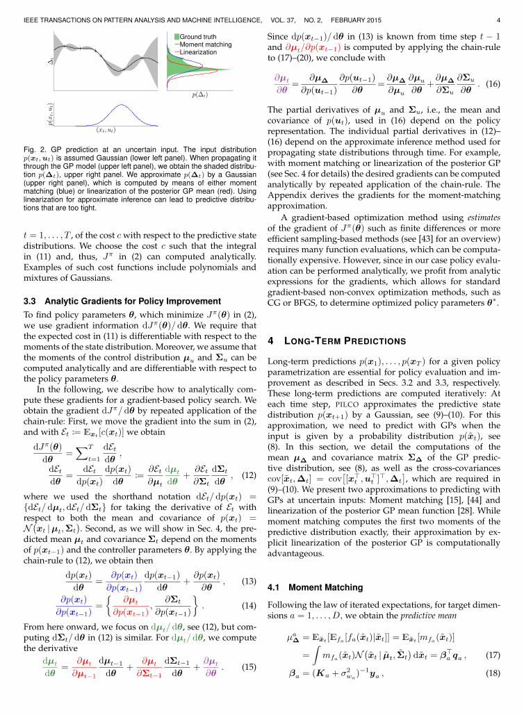
we integrate out both the random variable xt and the ran-dom function f , the latter one according to the posterior GPdistribution. Computing the exact predictive distribution in(8) is analytically intractable as illustrated in Fig. 2. Hence,we approximate p(∆t) by a Gaussian.
Assume the mean µ∆ and the covariance Σ∆ of thepredictive distribution p(∆t) are known3. Then, a Gaussianapproximation to the desired predictive distribution p(xt+1)is given as N
(xt+1 |µt+1,Σt+1
)with
µt+1 = µt + µ∆ , (9)Σt+1 = Σt + Σ∆ + cov[xt,∆t] + cov[∆t,xt] . (10)
Note that both µ∆ and Σ∆ are functions of the mean µuand the covariance Σu of the control signal.
To evaluate the expected long-term cost Jπ in (2), itremains to compute the expected values
Ext [c(xt)] =
∫c(xt)N
(xt |µt,Σt
)dxt , (11)
3. We will detail their computations in Secs. 4.1–4.2.
IEEE TRANSACTIONS ON PATTERN ANALYSIS AND MACHINE INTELLIGENCE, VOL. 37, NO. 2, FEBRUARY 2015 4
∆t
(xt, ut)
p(x
t,ut)
p(∆t)
Ground truthMoment matchingLinearization
Fig. 2. GP prediction at an uncertain input. The input distributionp(xt,ut) is assumed Gaussian (lower left panel). When propagating itthrough the GP model (upper left panel), we obtain the shaded distribu-tion p(∆t), upper right panel. We approximate p(∆t) by a Gaussian(upper right panel), which is computed by means of either momentmatching (blue) or linearization of the posterior GP mean (red). Usinglinearization for approximate inference can lead to predictive distribu-tions that are too tight.
t = 1, . . . , T , of the cost c with respect to the predictive statedistributions. We choose the cost c such that the integralin (11) and, thus, Jπ in (2) can computed analytically.Examples of such cost functions include polynomials andmixtures of Gaussians.
3.3 Analytic Gradients for Policy ImprovementTo find policy parameters θ, which minimize Jπ(θ) in (2),we use gradient information dJπ(θ)/ dθ. We require thatthe expected cost in (11) is differentiable with respect to themoments of the state distribution. Moreover, we assume thatthe moments of the control distribution µu and Σu can becomputed analytically and are differentiable with respect tothe policy parameters θ.
In the following, we describe how to analytically com-pute these gradients for a gradient-based policy search. Weobtain the gradient dJπ/ dθ by repeated application of thechain-rule: First, we move the gradient into the sum in (2),and with Et := Ext
[c(xt)] we obtain
dJπ(θ)
dθ=∑T
t=1
dEtdθ
,
dEtdθ
=dEt
dp(xt)
dp(xt)
dθ:=
∂Et∂µt
dµtdθ
+∂Et∂Σt
dΣt
dθ, (12)
where we used the shorthand notation dEt/ dp(xt) ={dEt/ dµt,dEt/dΣt} for taking the derivative of Et withrespect to both the mean and covariance of p(xt) =N(xt |µt,Σt
). Second, as we will show in Sec. 4, the pre-
dicted mean µt and covariance Σt depend on the momentsof p(xt−1) and the controller parameters θ. By applying thechain-rule to (12), we obtain then
dp(xt)
dθ=
∂p(xt)
∂p(xt−1)
dp(xt−1)
dθ+∂p(xt)
∂θ, (13)
∂p(xt)
∂p(xt−1)=
{∂µt
∂p(xt−1),
∂Σt
∂p(xt−1)
}. (14)
From here onward, we focus on dµt/dθ, see (12), but com-puting dΣt/ dθ in (12) is similar. For dµt/ dθ, we computethe derivative
dµtdθ
=∂µt∂µt−1
dµt−1dθ
+∂µt∂Σt−1
dΣt−1
dθ+∂µt∂θ
. (15)
Since dp(xt−1)/ dθ in (13) is known from time step t − 1and ∂µt/∂p(xt−1) is computed by applying the chain-ruleto (17)–(20), we conclude with
∂µt∂θ
=∂µ∆
∂p(ut−1)
∂p(ut−1)
∂θ=∂µ∆
∂µu
∂µu∂θ
+∂µ∆
∂Σu
∂Σu
∂θ. (16)
The partial derivatives of µu and Σu, i.e., the mean andcovariance of p(ut), used in (16) depend on the policyrepresentation. The individual partial derivatives in (12)–(16) depend on the approximate inference method used forpropagating state distributions through time. For example,with moment matching or linearization of the posterior GP(see Sec. 4 for details) the desired gradients can be computedanalytically by repeated application of the chain-rule. TheAppendix derives the gradients for the moment-matchingapproximation.
A gradient-based optimization method using estimatesof the gradient of Jπ(θ) such as finite differences or moreefficient sampling-based methods (see [43] for an overview)requires many function evaluations, which can be computa-tionally expensive. However, since in our case policy evalu-ation can be performed analytically, we profit from analyticexpressions for the gradients, which allows for standardgradient-based non-convex optimization methods, such asCG or BFGS, to determine optimized policy parameters θ∗.
4 LONG-TERM PREDICTIONS
Long-term predictions p(x1), . . . , p(xT ) for a given policyparametrization are essential for policy evaluation and im-provement as described in Secs. 3.2 and 3.3, respectively.These long-term predictions are computed iteratively: Ateach time step, PILCO approximates the predictive statedistribution p(xt+1) by a Gaussian, see (9)–(10). For thisapproximation, we need to predict with GPs when theinput is given by a probability distribution p(xt), see(8). In this section, we detail the computations of themean µ∆ and covariance matrix Σ∆ of the GP predic-tive distribution, see (8), as well as the cross-covariancescov[xt,∆t] = cov
[[x>t ,u
>t ]>,∆t
], which are required in
(9)–(10). We present two approximations to predicting withGPs at uncertain inputs: Moment matching [15], [44] andlinearization of the posterior GP mean function [28]. Whilemoment matching computes the first two moments of thepredictive distribution exactly, their approximation by ex-plicit linearization of the posterior GP is computationallyadvantageous.
4.1 Moment Matching
Following the law of iterated expectations, for target dimen-sions a = 1, . . . , D, we obtain the predictive mean
µa∆ = Ext [Efa [fa(xt)|xt]] = Ext [mfa(xt)]
=
∫mfa(xt)N
(xt | µt, Σt
)dxt = β>a qa , (17)
βa = (Ka + σ2wa
)−1ya , (18)

IEEE TRANSACTIONS ON PATTERN ANALYSIS AND MACHINE INTELLIGENCE, VOL. 37, NO. 2, FEBRUARY 2015 5
with qa = [qa1 , . . . , qan ]>. The entries of qa ∈ Rn arecomputed using standard results from multiplying andintegrating over Gaussians and are given by
qai =
∫ka(xi, xt)N
(xt | µt, Σt
)dxt (19)
= σ2fa |ΣtΛ
−1a + I|− 1
2 exp(− 1
2ν>i (Σt + Λa)−1νi
),
where we define
νi := (xi − µt) (20)
as the difference between the training input xi and the meanof the test input distribution p(xt,ut).
Computing the predictive covariance matrix Σ∆ ∈ RD×Drequires us to distinguish between diagonal elements σ2
aa
and off-diagonal elements σ2ab, a 6= b: Using the law of
total (co-)variance, we obtain for target dimensions a, b =1, . . . , D
σ2aa = Ext
[varf [∆a|xt]
]+Ef,xt
[∆2a]− (µa∆)2 , (21)
σ2ab = Ef,xt [∆a∆b]−µa∆µb∆ , a 6= b , (22)
respectively, where µa∆ is known from (17). The off-diagonal terms σ2
ab do not contain the additional termExt
[covf [∆a,∆b|xt]] because of the conditional indepen-dence assumption of the GP models: Different target dimen-sions do not covary for given xt.
We start the computation of the covariance matrix withthe terms that are common to both the diagonal and the off-diagonal entries: With p(xt) = N
(xt | µt, Σt
)and the law
of iterated expectations, we obtain
Ef,xt [∆a∆b] = Ext
[Ef [∆a|xt]Ef [∆b|xt]
](6)=
∫maf (xt)m
bf (xt)p(xt) dxt (23)
because of the conditional independence of ∆a and ∆b
given xt. Using the definition of the GP mean function in(6), we obtain
Ef,xt[∆a∆b] = β>aQβb , (24)
Q :=
∫ka(xt, X)> kb(xt, X)p(xt) dxt . (25)
Using standard results from Gaussian multiplications andintegration, we obtain the entries Qij of Q ∈ Rn×n
Qij = |R|−12 ka(xi, µt)kb(xj , µt) exp
(12z>ijT−1zij
)(26)
where we define
R := Σt(Λ−1a + Λ−1b ) + I , T := Λ−1a + Λ−1b + Σ
−1t ,
zij := Λ−1a νi + Λ−1b νj ,
with νi defined in (20). Hence, the off-diagonal entries ofΣ∆ are fully determined by (17)–(20), (22), and (24)–(26).
From (21), we see that the diagonal entries contain theadditional term
Ext
[varf [∆a|xt]
]=σ2
fa − tr((Ka+σ2
waI)−1Q
)+ σ2
wa(27)
with Q given in (26) and σ2wa
being the system noise vari-ance of the ath target dimension. This term is the expectedvariance of the function, see (7), under the distributionp(xt).
To obtain the cross-covariances cov[xt,∆t] in (10), wecompute the cross-covariance cov[xt,∆t] between an uncer-tain state-action pair xt ∼ N (µt, Σt) and the correspondingpredicted state difference xt+1 − xt = ∆t ∼ N (µ∆,Σ∆).This cross-covariance is given by
cov[xt,∆t] = Ext,f [xt∆>t ]−µtµ>∆ , (28)
where the components of µ∆ are given in (17), and µt isthe known mean of the input distribution of the state-actionpair at time step t.
Using the law of iterated expectation, for each statedimension a = 1, . . . , D, we compute Ext,f [xt ∆a
t ] as
Ext,f [xt ∆at ] = Ext
[xtEf [∆at |xt]] =
∫xtm
af (xt)p(xt) dxt
(6)=
∫xt( n∑i=1
βai kaf (xt, xi)
)p(xt) dxt , (29)
where the (posterior) GP mean function mf (xt) was rep-resented as a finite kernel expansion. Note that xi are thestate-action pairs, which were used to train the dynamicsGP model. By pulling the constant βai out of the integraland changing the order of summation and integration, weobtain
Ext,f [xt ∆at ]
=n∑i=1
βai
∫xt c1N (xt|xi,Λa)︸ ︷︷ ︸
=kaf (xt,xi)
N (xt|µt, Σt)︸ ︷︷ ︸p(xt)
dxt , (30)
where we define c1 := σ2fa
(2π)D+F
2 |Λa|12 with x ∈ RD+F ,
such that kaf (xt, xi) = c1N(xt | xi,Λa
)is an unnormal-
ized Gaussian probability distribution in xt, where xi,i = 1, . . . , n, are the GP training inputs. The product of thetwo Gaussians in (30) yields a new (unnormalized) Gaussianc−12 N
(xt |ψi,Ψ
)with
c−12 = (2π)−D+F
2 |Λa + Σt|−12
× exp(− 1
2 (xi − µt)>(Λa + Σt)−1(xi − µt)
),
Ψ = (Λ−1a + Σ−1t )−1 , ψi = Ψ(Λ−1a xi + Σ
−1t µt) .
By pulling all remaining variables, which are independentof xt, out of the integral in (30), the integral determinesthe expected value of the product of the two Gaussians, ψi.Hence, we obtain
Ext,f [xt ∆at ]=
∑n
i=1c1c−12 βaiψi , a = 1, . . . , D ,
covxt,f [xt,∆at ]=
∑n
i=1c1c−12 βaiψi−µtµa∆ , (31)
for all predictive dimensions a = 1, . . . , E. With c1c−12 =
qai , see (19), and ψi = Σt(Σt+Λa)−1xi+Λ(Σt+Λa)−1µtwe simplify (31) and obtain
covxt,f [xt,∆at ] =
n∑i=1
βaiqaiΣt(Σt+Λa)−1(xi−µt) , (32)
a = 1, . . . , E. The desired covariance cov[xt,∆t] is a D×Esubmatrix of the (D+F )×E cross-covariance computed into (32).
A visualization of the approximation of the predictivedistribution by means of exact moment matching is given inFig. 2.
IEEE TRANSACTIONS ON PATTERN ANALYSIS AND MACHINE INTELLIGENCE, VOL. 37, NO. 2, FEBRUARY 2015 6
4.2 Linearization of the Posterior GP Mean FunctionAn alternative way of approximating the predictive distri-bution p(∆t) by a Gaussian for xt ∼ N
(xt | µt, Σt
)is to
linearize the posterior GP mean function. Fig. 2 visualizesthe approximation by means of linearizing the posterior GPmean function.
The predicted mean is obtained by evaluating the posteriorGP mean in (5) at the mean µt of the input distribution, i.e.,
µa∆ = Ef [fa(µt)] = mfa(µt) = β>a ka(X, µt) , (33)
a = 1, . . . , E, where βa is given in (18).To compute the GP predictive covariance matrix Σ∆, we
explicitly linearize the posterior GP mean function aroundµt. By applying standard results for mapping Gaussian dis-tributions through linear models, the predictive covarianceis given by
Σ∆ = V ΣtV> + Σw , (34)
V =∂µ∆
∂µt= β>
∂k(X, µt)
∂µt. (35)
In (34), Σw is a diagonal matrix whose entries are the noisevariances σ2
waplus the model uncertainties varf [∆a
t |µt]evaluated at µt, see (7). This means, model uncertainty nolonger depends on the density of the data points. Instead itis assumed to be constant. Note that the moments computedin (33)–(34) are not exact.
The cross-covariance cov[xt,∆t] is given by ΣtV , whereV is defined in (35).
5 POLICY
In the following, we describe the desired properties ofthe policy within the PILCO learning framework. First, tocompute the long-term predictions p(x1), . . . , p(xT ) forpolicy evaluation, the policy must allow us to computea distribution over controls p(u) = p(π(x)) for a given(Gaussian) state distribution p(x). Second, in a realistic real-world application, the amplitudes of the control signals arebounded. Ideally, the learning system takes these constraintsexplicitly into account. In the following, we detail howPILCO implements these desiderata.
5.1 Predictive Distribution over ControlsDuring the long-term predictions, the states are given by aprobability distribution p(xt), t = 0, . . . , T . The probabilitydistribution of the state xt induces a predictive distributionp(ut) = p(π(xt)) over controls, even when the policy isdeterministic. We approximate the distribution over controlsusing moment matching, which is in many interesting casesanalytically tractable.
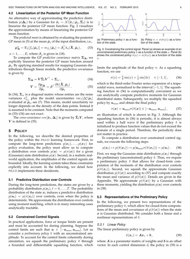
5.2 Constrained Control SignalsIn practical applications, force or torque limits are presentand must be accounted for during planning. Suppose thecontrol limits are such that u ∈ [−umax,umax]. Let usconsider a preliminary policy π with an unconstrained am-plitude. To account for the control limits coherently duringsimulation, we squash the preliminary policy π througha bounded and differentiable squashing function, which
−5 0 5
−1
0
1
2
x
π(x)
(a) Preliminary policy π as a func-tion of the state.
−5 0 5
−1
0
1
2
x
π(x)
(b) Policy π = σ(π(x)) as a func-tion of the state.
Fig. 3. Constraining the control signal. Panel (a) shows an example of anunconstrained preliminary policy π as a function of the state x. Panel (b)shows the constrained policy π(x) = σ(π(x)) as a function of the statex.
limits the amplitude of the final policy π. As a squashingfunction, we use
σ(x) = 98 sin(x) + 1
8 sin(3x) ∈ [−1, 1] , (36)
which is the third-order Fourier series expansion of a trape-zoidal wave, normalized to the interval [−1, 1]. The squash-ing function in (36) is computationally convenient as wecan analytically compute predictive moments for Gaussiandistributed states. Subsequently, we multiply the squashedpolicy by umax and obtain the final policy
π(x) = umaxσ(π(x)) ∈ [−umax,umax] , (37)
an illustration of which is shown in Fig. 3. Although thesquashing function in (36) is periodic, it is almost alwaysused within a half wave if the preliminary policy π isinitialized to produce function values that do not exceed thedomain of a single period. Therefore, the periodicity doesnot matter in practice.
To compute a distribution over constrained control sig-nals, we execute the following steps:
p(xt) 7→ p(π(xt)) 7→ p(umaxσ(π(xt))) = p(ut) . (38)
First, we map the Gaussian state distribution p(xt) throughthe preliminary (unconstrained) policy π. Thus, we requirea preliminary policy π that allows for closed-form com-putation of the moments of the distribution over controlsp(π(xt)). Second, we squash the approximate Gaussiandistribution p(π(x)) according to (37) and compute exactlythe mean and variance of p(π(x)). Details are given in theAppendix. We approximate p(π(x)) by a Gaussian withthese moments, yielding the distribution p(u) over controlsin (38).
5.3 Representations of the Preliminary PolicyIn the following, we present two representations of thepreliminary policy π, which allow for closed-form computa-tions of the mean and covariance of p(π(x)) when the statex is Gaussian distributed. We consider both a linear and anonlinear representations of π.
5.3.1 Linear PolicyThe linear preliminary policy is given by
π(x∗) = Ax∗ + b , (39)
where A is a parameter matrix of weights and b is an offsetvector. In each control dimension d, the policy in (39) is a
IEEE TRANSACTIONS ON PATTERN ANALYSIS AND MACHINE INTELLIGENCE, VOL. 37, NO. 2, FEBRUARY 2015 7
linear combination of the states (the weights are given bythe dth row in A) plus an offset bd.
The predictive distribution p(π(x∗)) for a state distribu-tion x∗ ∼ N (µ∗,Σ∗) is an exact Gaussian with mean andcovariance
Ex∗ [π(x∗)] = Aµ∗ + b , covx∗ [π(x∗)] = AΣ∗A> , (40)
respectively. A drawback of the linear policy is that it is notflexible. However, a linear controller can often be used forstabilization around an equilibrium.
5.3.2 Nonlinear Policy: Deterministic Gaussian Process
In the nonlinear case, we represent the preliminary policy πby
π(x∗)=N∑i=1
k(mi,x∗)(K + σ2πI)−1t = k(M ,x∗)
>α , (41)
where x∗ is a test input, α = (K + 0.01I)−1t, where tplays the role of a GP’s training targets. In (41), M =[m1, . . . ,mN ] are the centers of the (axis-aligned) Gaussianbasis functions
k(xp,xq) = exp(− 1
2 (xp − xq)>Λ−1(xp − xq)). (42)
We call the policy representation in (41) a deterministic GPwith a fixed number of N basis functions. Here, “determin-istic” means that there is no uncertainty about the under-lying function, that is, varπ[π(x)] = 0. Therefore, the de-terministic GP is a degenerate model, which is functionallyequivalent to a regularized RBF network. The deterministicGP is functionally equivalent to the posterior GP meanfunction in (6), where we set the signal variance to 1, see (42),and the noise variance to 0.01. As the preliminary policy willbe squashed through σ in (36) whose relevant support is theinterval [−π2 ,
π2 ], a signal variance of 1 is about right. Setting
additionally the noise standard deviation to 0.1 correspondsto fixing the signal-to-noise ratio of the policy to 10 and,hence, the regularization.
For a Gaussian distributed state x∗ ∼ N (µ∗,Σ∗), thepredictive mean of π(x∗) as defined in (41) is given as
Ex∗ [π(x∗)] = α>a Ex∗ [k(M ,x∗)]
= α>a
∫k(M ,x∗)p(x∗) dx∗ = α>a ra , (43)
where for i = 1, . . . , N and all policy dimensions a =1, . . . , F
rai = |Σ∗Λ−1a + I|−12
× exp(− 12 (µ∗ −mi)
>(Σ∗ + Λa)−1(µ∗ −mi)) .
The diagonal matrix Λa contains the squared length-scales`i, i = 1, . . . , D. The predicted mean in (43) is equivalent tothe standard predicted GP mean in (17).
For a, b = 1, . . . , F , the entries of the predictive covariancematrix are computed according to
covx∗ [πa(x∗), πb(x∗)]
= Ex∗ [πa(x∗)πb(x∗)]−Ex∗ [πa(x∗)]Ex∗ [πb(x∗)] ,
Algorithm 2 Computing the Successor State Distribution1: init: xt ∼ N (µt,Σt)2: Control distribution p(ut) = p(umaxσ(π(xt,θ)))3: Joint state-control distribution p(xt) = p(xt,ut)4: Predictive GP distribution of change in state p(∆t)5: Distribution of successor state p(xt+1)
where Ex∗ [π{a,b}(x∗)] is given in (43). Hence, we focus onthe term Ex∗ [πa(x∗)πb(x∗)], which for a, b = 1, . . . , F isgiven by
Ex∗ [πa(x∗)πb(x∗)] = α>a Ex∗ [ka(M ,x∗)kb(M ,x∗)>]αb
= α>aQαb .
For i, j = 1, . . . , N , we compute the entries of Q as
Qij =
∫ka(mi,x∗)kb(mj ,x∗)p(x∗) dx∗
= ka(mi,µ∗)kb(mj ,µ∗)|R|− 1
2 exp( 12z>ijT−1zij) ,
R = Σ∗(Λ−1a + Λ−1b ) + I , T = Λ−1a + Λ−1b + Σ−1∗ ,
zij = Λ−1a (µ∗ −mi) + Λ−1b (µ∗ −mj) .
Combining this result with (43) fully determines the predic-tive covariance matrix of the preliminary policy.
Unlike the predictive covariance of a probabilistic GP,see (21)–(22), the predictive covariance matrix of the deter-ministic GP does not comprise any model uncertainty in itsdiagonal entries.
5.4 Policy ParametersIn the following, we describe the policy parameters for boththe linear and the nonlinear policy4.
5.4.1 Linear PolicyThe linear policy in (39) possesses D + 1 parameters percontrol dimension: For control dimension d there are Dweights in the dth row of the matrix A. One additionalparameter originates from the offset parameter bd.
5.4.2 Nonlinear PolicyThe parameters of the deterministic GP in (41) are thelocations M of the centers (DN parameters), the (shared)length-scales of the Gaussian basis functions (D length-scaleparameters per target dimension), and the N targets t pertarget dimension. In the case of multivariate controls, thebasis function centers M are shared.
5.5 Computing the Successor State DistributionAlg. 2 summarizes the computational steps required tocompute the successor state distribution p(xt+1) from p(xt).The computation of a distribution over controls p(ut) fromthe state distribution p(xt) requires two steps: First, for aGaussian state distribution p(xt) at time t a Gaussian ap-proximation of the distribution p(π(xt)) of the preliminarypolicy is computed analytically. Second, the preliminary
4. For notational convenience, with a (non)linear policy we meanthe (non)linear preliminary policy π mapped through the squashingfunction σ and subsequently multiplied by umax.

IEEE TRANSACTIONS ON PATTERN ANALYSIS AND MACHINE INTELLIGENCE, VOL. 37, NO. 2, FEBRUARY 2015 8
policy is squashed through σ and an approximate Gaussiandistribution of p(umaxσ(π(xt))) is computed analytically in(38) using results from the Appendix. Third, we analyticallycompute a Gaussian approximation to the joint distributionp(xt,ut) = p(xt, π(xt)). For this, we compute (a) a Gaus-sian approximation to the joint distribution p(xt, π(xt)),which is exact if π is linear, and (b) an approximate fullyjoint Gaussian distribution p(xt, π(xt),ut). We obtain cross-covariance information between the state xt and the controlsignal ut = umaxσ(π(xt)) via
cov[xt,ut]=cov[xt, π(xt)]cov[π(xt), π(xt)]−1cov[π(xt),ut] ,
where we exploit the conditional independence of xt andut given π(xt). Then, we integrate π(xt) out to obtain thedesired joint distribution p(xt,ut). This leads to an approx-imate Gaussian joint probability distribution p(xt,ut) =p(xt, π(xt)) = p(xt). Fourth, with the approximate Gaus-sian input distribution p(xt), the distribution p(∆t) of thechange in state is computed using the results from Sec. 4.Finally, the mean and covariance of a Gaussian approxima-tion of the successor state distribution p(xt+1) are given by(9) and (10), respectively.
All required computations can be performed analyticallybecause of the choice of the Gaussian covariance functionfor the GP dynamics model, see (3), the representations ofthe preliminary policy π, see Sec. 5.3, and the choice of thesquashing function, see (36).
6 COST FUNCTION
In our learning set-up, we use a cost function that solelypenalizes the Euclidean distance d of the current state to thetarget state. Using only distance penalties is often sufficientto solve a task: Reaching a target xtarget with high speednaturally leads to overshooting and, thus, to high long-termcosts. In particular, we use the generalized binary saturatingcost
c(x) = 1− exp(− 1
2σ2cd(x,xtarget)
2)∈ [0, 1] , (44)
which is locally quadratic but saturates at unity for largedeviations d from the desired target xtarget. In (44), thegeometric distance from the state x to the target state isdenoted by d, and the parameter σc controls the width ofthe cost function.5
In classical control, typically a quadratic cost is assumed.However, a quadratic cost tends to focus attention on theworst deviation from the target state along a predictedtrajectory. In the early stages of learning the predictive un-certainty is large and, therefore, the policy gradients, whichare described in Sec. 3.3 become less useful. Therefore, weuse the saturating cost in (44) as a default within the PILCOlearning framework.
The immediate cost in (44) is an unnormalized Gaussianwith mean xtarget and variance σ2
c , subtracted from unity.
5. In the context of sensorimotor control, the saturating cost functionin (44) resembles the cost function in human reasoning as experimen-tally validated by [31].
−1.5 −1 −0.5 0 0.5 1 1.50
0.5
1
1.5
2
2.5
state
cost functionpeaked state distributionwide state distribution
(a) When the mean of the state isfar away from the target, uncertainstates (red, dashed-dotted) arepreferred to more certain stateswith a more peaked distribution(black, dashed). This leads to ini-tial exploration.
−1.5 −1 −0.5 0 0.5 1 1.50
0.5
1
1.5
2
2.5
state
cost functionpeaked state distributionwide state distribution
(b) When the mean of the stateis close to the target, peakedstate distributions (black, dashed)cause less expected cost and,thus, are preferable to more uncer-tain states (red, dashed-dotted),leading to exploitation close to thetarget.
Fig. 4. Automatic exploration and exploitation with the saturating costfunction (blue, solid). The x-axes describe the state space. The targetstate is the origin.
Therefore, the expected immediate cost can be computedanalytically according to
Ex[c(x)] =
∫c(x)p(x) dx (45)
= 1−∫
exp(− 1
2 (x− xtarget)>T−1(x− xtarget)
)p(x) dx ,
where T−1 is the precision matrix of the unnormalizedGaussian in (45). If the state x has the same representationas the target vector, T−1 is a diagonal matrix with entrieseither unity or zero, scaled by 1/σ2
c . Hence, for x ∼ N (µ,Σ)we obtain the expected immediate cost
Ex[c(x)] = 1− |I + ΣT−1|−1/2
× exp(− 12 (µ− xtarget)
>S1(µ− xtarget)) , (46)
S1 := T−1(I + ΣT−1)−1 . (47)
The partial derivatives ∂∂µtExt
[c(xt)],∂∂Σt
Ext[c(xt)] of the
immediate cost with respect to the mean and the covarianceof the state distribution p(xt) = N (µt,Σt), which arerequired to compute the policy gradients analytically, aregiven by
∂Ext [c(xt)]
∂µt= −Ext
[c(xt)] (µt − xtarget)>S1 , (48)
∂Ext [c(xt)]
∂Σt= 1
2Ext[c(xt)] (49)
×(S1(µt − xtarget)(µt − xtarget)
> − I)S1 ,
respectively, where S1 is given in (47).
6.1 Exploration and Exploitation
The saturating cost function in (44) allows for a naturalexploration when the policy aims to minimize the expectedlong-term cost in (2). This property is illustrated in Fig. 4for a single time step where we assume a Gaussian statedistribution p(xt). If the mean of p(xt) is far away fromthe target xtarget, a wide state distribution is more likelyto have substantial tails in some low-cost region than amore peaked distribution as shown in Fig. 4(a). In the

IEEE TRANSACTIONS ON PATTERN ANALYSIS AND MACHINE INTELLIGENCE, VOL. 37, NO. 2, FEBRUARY 2015 9
early stages of learning, the predictive state uncertainty islargely due to propagating model uncertainties forward. Ifwe predict a state distribution in a high-cost region, the sat-urating cost then leads to automatic exploration by favoringuncertain states, i.e., states in regions far from the targetwith a poor dynamics model. When visiting these regionsduring interaction with the physical system, subsequentmodel learning reduces the model uncertainty locally. In thesubsequent policy evaluation, PILCO will predict a tighterstate distribution in the situations described in Fig. 4.
If the mean of the state distribution is close to the target asin Fig. 4(b), wide distributions are likely to have substantialtails in high-cost regions. By contrast, the mass of a peakeddistribution is more concentrated in low-cost regions. In thiscase, the policy prefers peaked distributions close to thetarget, leading to exploitation.
To summarize, combining a probabilistic dynamicsmodel, Bayesian inference, and a saturating cost leads toautomatic exploration as long as the predictions are far fromthe target—even for a policy, which greedily minimizes theexpected cost. Once close to the target, the policy does notsubstantially deviate from a confident trajectory that leadsthe system close to the target.6
7 EXPERIMENTAL RESULTS
In this section, we assess PILCO’s key properties and showthat PILCO scales to high-dimensional control problems.Moreover, we demonstrate the hardware applicability ofour learning framework on two real systems. In all cases,PILCO followed the steps outlined in Alg. 1. To reducethe computational burden, we used the sparse GP methodof [50] after 300 collected data points.
7.1 Evaluation of Key PropertiesIn the following, we assess the quality of the approximateinference method used for long-term predictions in terms ofcomputational demand and learning speed. Moreover, weshed some light on the quality of the Gaussian approxima-tions of the predictive state distributions and the importanceof Bayesian averaging. For these assessments, we appliedPILCO to two nonlinear control tasks, which are introducedin the following.
7.1.1 Task DescriptionsWe considered two simulated tasks (double-pendulumswing-up, cart-pole swing-up) to evaluate important prop-erties of the PILCO policy search framework: learning speed,quality of approximate inference, importance of Bayesianaveraging, and hardware applicability. In the following webriefly introduce the experimental set-ups.
7.1.1.1 Double-Pendulum Swing-Up with Two Ac-tuators: The double pendulum system is a two-link robotarm with two actuators, see Fig. 5. The state x is given by theangles θ1, θ2 and the corresponding angular velocities θ1, θ2of the inner and outer link, respectively, measured frombeing upright. Each link was of length 1 m and mass 0.5 kg.Both torques u1 and u2 were constrained to [−3, 3] Nm.The control signal could be changed every 100 ms. In the
6. Code is available at http://mloss.org/software/view/508/.
target
u1
u2
d
Fig. 5. Double pendulum with two actuators applying torques u1 and u2.The cost function penalizes the distance d to the target.
meantime it was constant (zero-order-hold control). Theobjective was to learn a controller that swings the doublependulum up from an initial distribution p(x0) aroundµ0 = [π, π, 0, 0]> and balances it in the inverted positionwith θ1 = 0 = θ2. The prediction horizon was 2.5 s.
The task is challenging since its solution requires the in-terplay of two correlated control signals. The challenge is toautomatically learn this interplay from experience. To solvethe double pendulum swing-up task, a nonlinear policy isrequired. Thus, we parametrized the preliminary policy as adeterministic GP, see (41), with 100 basis functions resultingin 812 policy parameters. We chose the saturating immediatecost in (44), where the Euclidean distance between theupright position and the tip of the outer link was penalized.We chose the cost width σc = 0.5, which means that the tipof the outer pendulum had to cross horizontal to achieve animmediate cost smaller than unity.
7.1.1.2 Cart-Pole Swing-Up: The cart-pole systemconsists of a cart running on a track and a freely swing-ing pendulum attached to the cart. The state of the sys-tem is the position x of the cart, the velocity x of thecart, the angle θ of the pendulum measured from hangingdownward, and the angular velocity θ. A horizontal forceu ∈ [−10, 10] N could be applied to the cart. The objectivewas to learn a controller to swing the pendulum up fromaround µ0 = [x0, x0, θ0, θ0]> = [0, 0, 0, 0]> and to balanceit in the inverted position in the middle of the track, i.e.,around xtarget = [0, ∗, π, ∗]>. Since a linear controller is notcapable of solving the task [45], PILCO learned a nonlinearstate-feedback controller based on a deterministic GP with50 basis functions (see Sec. 5.3.2), resulting in 305 policyparameters to be learned.
In our simulation, we set the masses of the cart andthe pendulum to 0.5 kg each, the length of the pendulumto 0.5 m, and the coefficient of friction between cart andground to 0.1 Ns/m. The prediction horizon was set to 2.5 s.The control signal could be changed every 100 ms. In themeantime, it was constant (zero-order-hold control). Theonly knowledge employed about the system was the lengthof the pendulum to find appropriate orders of magnitudeto set the sampling frequency (10 Hz) and the standarddeviation of the cost function (σc = 0.25 m), requiring thetip of the pendulum to move above horizontal not to incurfull cost.
IEEE TRANSACTIONS ON PATTERN ANALYSIS AND MACHINE INTELLIGENCE, VOL. 37, NO. 2, FEBRUARY 2015 10
5 10 15 20 25 30 35 40 45 50
10−2
100
102
State space dimensionality
Com
puta
tion tim
e in s
100 Training Points250 Training Points500 Training Points1000 Training Points
(a) Linearizing the mean function.
5 10 15 20 25 30 35 40 45 50
10−2
100
102
State space dimensionality
Com
puta
tion tim
e in s
100 Training Points250 Training Points500 Training Points1000 Training Points
(b) Moment matching.
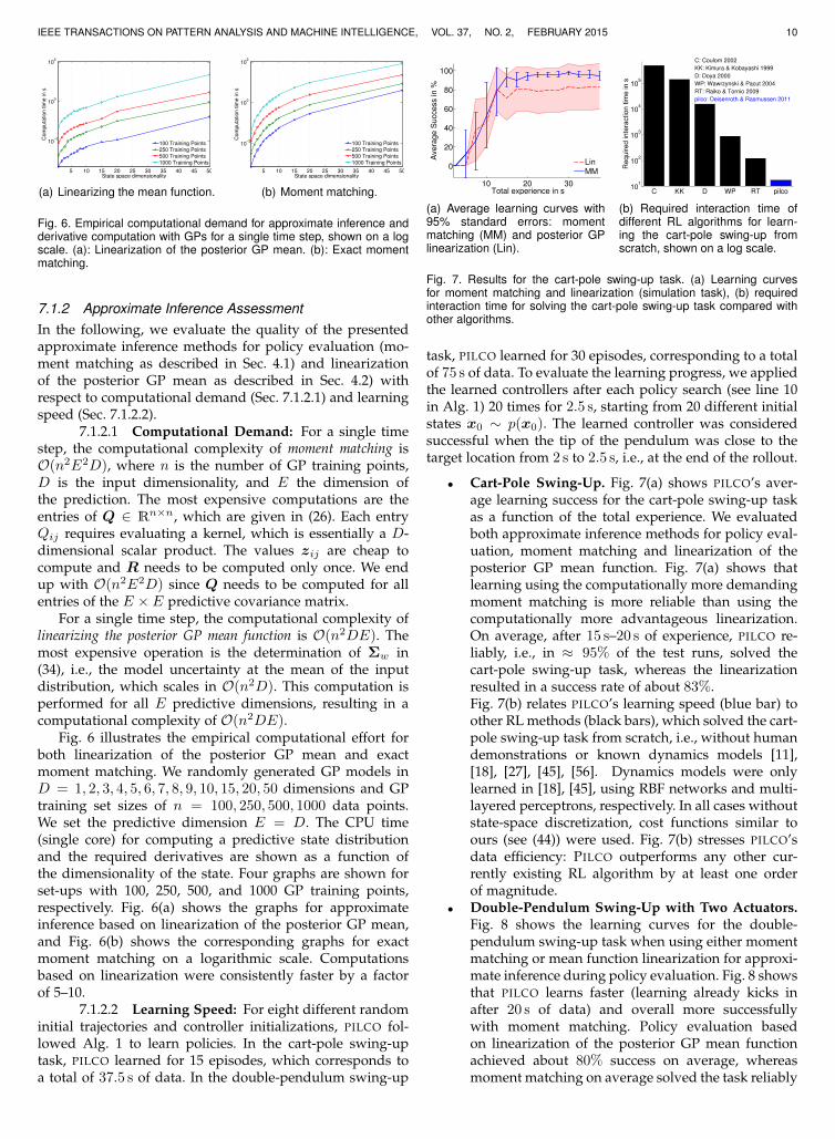
Fig. 6. Empirical computational demand for approximate inference andderivative computation with GPs for a single time step, shown on a logscale. (a): Linearization of the posterior GP mean. (b): Exact momentmatching.
7.1.2 Approximate Inference AssessmentIn the following, we evaluate the quality of the presentedapproximate inference methods for policy evaluation (mo-ment matching as described in Sec. 4.1) and linearizationof the posterior GP mean as described in Sec. 4.2) withrespect to computational demand (Sec. 7.1.2.1) and learningspeed (Sec. 7.1.2.2).
7.1.2.1 Computational Demand: For a single timestep, the computational complexity of moment matching isO(n2E2D), where n is the number of GP training points,D is the input dimensionality, and E the dimension ofthe prediction. The most expensive computations are theentries of Q ∈ Rn×n, which are given in (26). Each entryQij requires evaluating a kernel, which is essentially a D-dimensional scalar product. The values zij are cheap tocompute and R needs to be computed only once. We endup with O(n2E2D) since Q needs to be computed for allentries of the E × E predictive covariance matrix.
For a single time step, the computational complexity oflinearizing the posterior GP mean function is O(n2DE). Themost expensive operation is the determination of Σw in(34), i.e., the model uncertainty at the mean of the inputdistribution, which scales in O(n2D). This computation isperformed for all E predictive dimensions, resulting in acomputational complexity of O(n2DE).
Fig. 6 illustrates the empirical computational effort forboth linearization of the posterior GP mean and exactmoment matching. We randomly generated GP models inD = 1, 2, 3, 4, 5, 6, 7, 8, 9, 10, 15, 20, 50 dimensions and GPtraining set sizes of n = 100, 250, 500, 1000 data points.We set the predictive dimension E = D. The CPU time(single core) for computing a predictive state distributionand the required derivatives are shown as a function ofthe dimensionality of the state. Four graphs are shown forset-ups with 100, 250, 500, and 1000 GP training points,respectively. Fig. 6(a) shows the graphs for approximateinference based on linearization of the posterior GP mean,and Fig. 6(b) shows the corresponding graphs for exactmoment matching on a logarithmic scale. Computationsbased on linearization were consistently faster by a factorof 5–10.
7.1.2.2 Learning Speed: For eight different randominitial trajectories and controller initializations, PILCO fol-lowed Alg. 1 to learn policies. In the cart-pole swing-uptask, PILCO learned for 15 episodes, which corresponds toa total of 37.5 s of data. In the double-pendulum swing-up
10 20 30
0
20
40
60
80
100
Total experience in s
Ave
rag
e S
ucce
ss in
%
LinMM
(a) Average learning curves with95% standard errors: momentmatching (MM) and posterior GPlinearization (Lin).
C KK D WP RT pilco10
1
102
103
104
105
C: Coulom 2002
KK: Kimura & Kobayashi 1999
D: Doya 2000
WP: Wawrzynski & Pacut 2004
RT: Raiko & Tornio 2009
pilco: Deisenroth & Rasmussen 2011
Required inte
raction tim
e in s
(b) Required interaction time ofdifferent RL algorithms for learn-ing the cart-pole swing-up fromscratch, shown on a log scale.
Fig. 7. Results for the cart-pole swing-up task. (a) Learning curvesfor moment matching and linearization (simulation task), (b) requiredinteraction time for solving the cart-pole swing-up task compared withother algorithms.
task, PILCO learned for 30 episodes, corresponding to a totalof 75 s of data. To evaluate the learning progress, we appliedthe learned controllers after each policy search (see line 10in Alg. 1) 20 times for 2.5 s, starting from 20 different initialstates x0 ∼ p(x0). The learned controller was consideredsuccessful when the tip of the pendulum was close to thetarget location from 2 s to 2.5 s, i.e., at the end of the rollout.
• Cart-Pole Swing-Up. Fig. 7(a) shows PILCO’s aver-age learning success for the cart-pole swing-up taskas a function of the total experience. We evaluatedboth approximate inference methods for policy eval-uation, moment matching and linearization of theposterior GP mean function. Fig. 7(a) shows thatlearning using the computationally more demandingmoment matching is more reliable than using thecomputationally more advantageous linearization.On average, after 15 s–20 s of experience, PILCO re-liably, i.e., in ≈ 95% of the test runs, solved thecart-pole swing-up task, whereas the linearizationresulted in a success rate of about 83%.Fig. 7(b) relates PILCO’s learning speed (blue bar) toother RL methods (black bars), which solved the cart-pole swing-up task from scratch, i.e., without humandemonstrations or known dynamics models [11],[18], [27], [45], [56]. Dynamics models were onlylearned in [18], [45], using RBF networks and multi-layered perceptrons, respectively. In all cases withoutstate-space discretization, cost functions similar toours (see (44)) were used. Fig. 7(b) stresses PILCO’sdata efficiency: PILCO outperforms any other cur-rently existing RL algorithm by at least one orderof magnitude.
• Double-Pendulum Swing-Up with Two Actuators.Fig. 8 shows the learning curves for the double-pendulum swing-up task when using either momentmatching or mean function linearization for approxi-mate inference during policy evaluation. Fig. 8 showsthat PILCO learns faster (learning already kicks inafter 20 s of data) and overall more successfullywith moment matching. Policy evaluation basedon linearization of the posterior GP mean functionachieved about 80% success on average, whereasmoment matching on average solved the task reliably

IEEE TRANSACTIONS ON PATTERN ANALYSIS AND MACHINE INTELLIGENCE, VOL. 37, NO. 2, FEBRUARY 2015 11
20 40 60
0
20
40
60
80
100
Total experience in s
Ave
rag
e S
ucce
ss in
%
LinMM
Fig. 8. Average success as a function of the total data used for learning(double pendulum swing-up). The blue error bars show the 95% con-fidence bounds of the standard error for the moment matching (MM)approximation, the red area represents the corresponding confidencebounds of success when using approximate inference by means oflinearizing the posterior GP mean (Lin).
0 0.5 1 1.5 2 2.5
−8
−6
−4
−2
0
2
4
6
Time in s
Angle
inner
pendulu
m in r
ad
Actual trajectories
Predicted trajectory
(a) Early stage of learning.
0 0.5 1 1.5 2 2.5
0
0.5
1
1.5
2
2.5
3
3.5
Time in s
An
gle
in
ne
r p
en
du
lum
in
ra
d
Actual trajectories
Predicted trajectory
(b) After successful learning.
Fig. 9. Long-term predictive (Gaussian) distributions during planning(shaded) and sample rollouts (red). (a) In the early stages of learning,the Gaussian approximation is a suboptimal choice. (b) PILCO learned acontroller such that the Gaussian approximations of the predictive statesare good. Note the different scales in (a) and (b).
after about 50 s of data with a success rate ≈ 95%.
Summary. We have seen that both approximate inferencemethods have pros and cons: Moment matching requiresmore computational resources than linearization, but learnsfaster and more reliably. The reason why linearization didnot reliably succeed in learning the tasks is that it getsrelatively easily stuck in local minima, which is largely aresult of underestimating predictive variances, an exampleof which is given in Fig. 2. Propagating too confident pre-dictions over a longer horizon often worsens the problem.Hence, in the following, we focus solely on the momentmatching approximation.
7.1.3 Quality of the Gaussian ApproximationPILCO strongly relies on the quality of approximate infer-ence, which is used for long-term predictions and policyevaluation, see Sec. 4. We already saw differences betweenlinearization and moment matching; however, both meth-ods approximate predictive distributions by a Gaussian.Although we ultimately cannot answer whether this ap-proximation is good under all circumstances, we will shedsome light on this issue.
Fig. 9 shows a typical example of the angle of the innerpendulum of the double pendulum system where, in theearly stages of learning, the Gaussian approximation to themulti-step ahead predictive distribution is not ideal. Thetrajectory distribution of a set of rollouts (red) is multi-modal. PILCO deals with this inappropriate modeling by
TABLE 1Average learning success with learned nonparametric (NP) transition
models (cart-pole swing-up).
Bayesian NP model Deterministic NP modelLearning success 94.52% 0%
learning a controller that forces the actual trajectories into aunimodal distribution such that a Gaussian approximationis appropriate, Fig. 9(b).
We explain this behavior as follows: Assuming thatPILCO found different paths that lead to a target, a wideGaussian distribution is required to capture the variability ofthe bimodal distribution. However, when computing the ex-pected cost using a quadratic or saturating cost, for example,uncertainty in the predicted state leads to higher expectedcost, assuming that the mean is close to the target. Therefore,PILCO uses its ability to choose control policies to push themarginally multimodal trajectory distribution into a singlemode—from the perspective of minimizing expected costwith limited expressive power, this approach is desirable.Effectively, learning good controllers and models goes handin hand with good Gaussian approximations.
7.1.4 Importance of Bayesian AveragingModel-based RL greatly profits from the flexibility of non-parametric models as motivated in Sec. 2. In the follow-ing, we have a closer look at whether Bayesian modelsare strictly necessary as well. In particular, we evaluatedwhether Bayesian averaging is necessary for successfullylearning from scratch. To do so, we considered the cart-poleswing-up task with two different dynamics models: first, thestandard nonparametric Bayesian GP model, second, a non-parametric deterministic GP model, i.e., a GP where we con-sidered only the posterior mean, but discarded the posteriormodel uncertainty when doing long-term predictions. Wealready described a similar kind of function representationto learn a deterministic policy, see Sec. 5.3.2. The differenceto the policy is that in this section the deterministic GP isstill nonparametric (new basis functions are added if weget more data), whereas the number of basis functions inthe policy is fixed. However, the deterministic GP is nolonger probabilistic because of the loss of model uncertainty,which also results in a degenerate model. Note that westill propagate uncertainties resulting from the initial statedistribution p(x0) forward.
Tab. 1 shows the average learning success of swingingthe pendulum up and balancing it in the inverted positionin the middle of the track. We used moment matching forapproximate inference, see Sec. 4. Tab. 1 shows that learningis only successful when model uncertainties are taken intoaccount during long-term planning and control learning,which strongly suggests Bayesian nonparametric models inmodel-based RL.
The reason why model uncertainties must be appro-priately taken into account is the following: In the earlystages of learning, the learned dynamics model is basedon a relatively small data set. States close to the target areunlikely to be observed when applying random controls.Therefore, the model must extrapolate from the current setof observed states. This requires to predict function values in

IEEE TRANSACTIONS ON PATTERN ANALYSIS AND MACHINE INTELLIGENCE, VOL. 37, NO. 2, FEBRUARY 2015 12
frame
flywheel
wheel
(a) Robotic unicy-cle.
1 2 3 4 50
20
40
60
80
100
time in s
dis
tance d
istr
ibution in %
d ≤ 3 cm d ∈ (3,10] cm d ∈ (10,50] cm d > 50cm
(b) Histogram (after 1,000 test runs) of thedistances of the flywheel from being upright.
Fig. 10. Robotic unicycle system and simulation results. The state spaceis R12, the control space R2.
regions with large posterior model uncertainty. Dependingon the choice of the deterministic function (we chose theMAP estimate), the predictions (point estimates) are verydifferent. Iteratively predicting state distributions ends upin predicting trajectories, which are essentially arbitrary andnot close to the target state either, resulting in vanishingpolicy gradients.
7.2 Scaling to Higher Dimensions: Unicycling
We applied PILCO to learning to ride a 5-DoF unicyclewith x ∈ R12 and u ∈ R2 in a realistic simulationof the one shown in Fig. 10(a). The unicycle was 0.76 mhigh and consisted of a 1 kg wheel, a 23.5 kg frame, anda 10 kg flywheel mounted perpendicularly to the frame.Two torques could be applied to the unicycle: The firsttorque |uw| ≤ 10 Nm was applied directly on the wheelto mimic a human rider using pedals. The torque producedlongitudinal and tilt accelerations. Lateral stability of thewheel could be maintained by steering the wheel towardthe falling direction of the unicycle and by applying a torque|ut| ≤ 50 Nm to the flywheel. The dynamics of the roboticunicycle were described by 12 coupled first-order ODEs,see [24].
The objective was to learn a controller for riding the uni-cycle, i.e., to prevent it from falling. To solve the balancingtask, we used the linear preliminary policy π(x,θ) = Ax+bwith θ = {A, b} ∈ R28. The covariance Σ0 of the initialstate was 0.252I allowing each angle to be off by about 30◦
(twice the standard deviation).PILCO differs from conventional controllers in that it
learns a single controller for all control dimensions jointly.Thus, PILCO takes the correlation of all control and state di-mensions into account during planning and control. Learn-ing separate controllers for each control variable is oftenunsuccessful [37].
PILCO required about 20 trials, corresponding to anoverall experience of about 30 s, to learn a dynamics modeland a controller that keeps the unicycle upright. A trialwas aborted when the turntable hit the ground, whichhappened quickly during the five random trials used for ini-tialization. Fig. 10(b) shows empirical results after 1,000 testruns with the learned policy: Differently-colored bars showthe distance of the flywheel from a fully upright position.Depending on the initial configuration of the angles, the
unicycle had a transient phase of about a second. After 1.2 s,either the unicycle had fallen or the learned controller hadmanaged to balance it very closely to the desired uprightposition. The success rate was approximately 93%; bringingthe unicycle upright from extreme initial configurations wassometimes impossible due to the torque constraints.
7.3 Hardware Tasks
In the following, we present results from [15], [16], wherewe successfully applied the PILCO policy search frameworkto challenging control and robotics tasks, respectively. Itis important to mention that no task-specific modificationswere necessary, besides choosing a controller representationand defining an immediate cost function. In particular, weused the same standard GP priors for learning the forwarddynamics models.
7.3.1 Cart-Pole Swing-Up
As described in [15], PILCO was applied to learning to con-trol the real cart-pole system, see Fig. 11, developed by [26].The masses of the cart and pendulum were 0.7 kg and0.325 kg, respectively. A horizontal force u ∈ [−10, 10] Ncould be applied to the cart.
PILCO successfully learned a sufficiently good dynam-ics model and a good controller fully automatically inonly a handful of trials and a total experience of 17.5 s,which also confirms the learning speed of the simu-lated cart-pole system in Fig. 7(b) despite the fact thatthe parameters of the system dynamics (masses, pendu-lum length, friction, delays, stiction, etc.) are different.Snapshots of a 20 s test trajectory are shown in Fig. 11;a video of the entire learning process is available athttp://www.youtube.com/user/PilcoLearner.
7.3.2 Controlling a Low-Cost Robotic Manipulator
We applied PILCO to make a low-precision robotic arm learnto stack a tower of foam blocks—fully autonomously [16].For this purpose, we used the lightweight robotic manip-ulator by Lynxmotion [1] shown in Fig. 12. The arm costsapproximately $370 and possesses six controllable degreesof freedom: base rotate, three joints, wrist rotate, and agripper (open/close). The plastic arm was controllable bycommanding both a desired configuration of the six servosvia their pulse durations and the duration for executing thecommand. The arm was very noisy: Tapping on the basemade the end effector swing in a radius of about 2 cm. Thesystem noise was particularly pronounced when moving thearm vertically (up/down). Additionally, the servo motorshad some play.
Knowledge about the joint configuration of the robot wasnot available. We used a PrimeSense depth camera [2] as anexternal sensor for visual tracking the block in the gripperof the robot. The camera was identical to the Kinect sensor,providing a synchronized depth image and a 640×480 RGBimage at 30 Hz. Using structured infrared light, the cameradelivered useful depth information of objects in a range ofabout 0.5 m–5 m. The depth resolution was approximately1 cm at a distance of 2 m [2].

IEEE TRANSACTIONS ON PATTERN ANALYSIS AND MACHINE INTELLIGENCE, VOL. 37, NO. 2, FEBRUARY 2015 13
1 2 3 4 5 6
Fig. 11. Real cart-pole system [15]. Snapshots of a controlled trajectory of 20 s length after having learned the task. To solve the swing-up plusbalancing, PILCO required only 17.5 s of interaction with the physical system.
Fig. 12. Low-cost robotic arm by Lynxmotion [1]. The manipulator doesnot provide any pose feedback. Hence, PILCO learns a controller directlyin the task space using visual feedback from a PrimeSense depthcamera.
Every 500 ms, the robot used the 3D center of the blockin its gripper as the state x ∈ R3 to compute a continuous-valued control signal u ∈ R4, which comprised the com-manded pulse widths for the first four servo motors. Wristrotation and gripper opening/closing were not learned. Forblock tracking we used real-time (50 Hz) color-based regiongrowing to estimate the extent and 3D center of the object,which was used as the state x ∈ R3 by PILCO.
As an initial state distribution, we chose p(x0) =N(x0 |µ0,Σ0
)with µ0 being a single noisy measurement
of the 3D camera coordinates of the block in the gripperwhen the robot was in its initial configuration. The initialcovariance Σ0 was diagonal, where the 95%-confidencebounds were the edge length b of the block. Similarly, thetarget state was set based on a single noisy measurementusing the PrimeSense camera. We used linear preliminarypolicies, i.e., π(x) = u = Ax + b, and initialized thecontroller parameters θ = {A, b} ∈ R16 to zero. TheEuclidean distance d of the end effector from the camera wasapproximately 0.7 m–2.0 m, depending on the robot’s con-figuration. The cost function in (44) penalized the Euclideandistance of the block in the gripper from its desired targetlocation on top of the current tower. Both the frequency atwhich the controls were changed and the time discretizationwere set to 2 Hz; the planning horizon T was 5 s. After 5 s,the robot opened the gripper and released the block.
We split the task of building a tower into learningindividual controllers for each target block B2–B6 (bottomto top), see Fig. 12, starting from a configuration, in whichthe robot arm was upright. All independently trained con-trollers shared the same initial trial.
The motion of the block in the end effector was modeledby GPs. The inferred system noise standard deviations,which comprised stochasticity of the robot arm, synchro-nization errors, delays, image processing errors, etc., rangedfrom 0.5 cm to 2.0 cm. Here, the y-coordinate, which corre-sponded to the height, suffered from larger noise than the
other coordinates. The reason for this is that the robot move-ment was particularly jerky in the up/down movements.These learned noise levels were in the right ballpark sincethey were slightly larger than the expected camera noise [2].The signal-to-noise ratio in our experiments ranged from 2to 6.
A total of ten learning-interacting iterations (includingthe random initial trial) generally sufficed to learn both goodforward models and good controllers as shown in Fig. 13(a),which displays the learning curve for a typical trainingsession, averaged over ten test runs after each learningstage and all blocks B2–B6. The effects of learning becamenoticeable after about four learning iterations. After 10learning iterations, the block in the gripper was expected tobe very close (approximately at noise level) to the target. Therequired interaction time sums up to only 50 s per controllerand 230 s in total (the initial random trial is counted onlyonce). This speed of learning is difficult to achieve by otherRL methods that learn from scratch as shown in Sec. 7.1.1.2.
Fig. 13(b) gives some insights into the quality of thelearned forward model after 10 controlled trials. It showsthe marginal predictive distributions and the actual trajec-tories of the block in the gripper. The robot learned to payattention to stabilizing the y-coordinate quickly: Moving thearm up/down caused relatively large “system noise” as thearm was quite jerky in this direction: In the y-coordinatethe predictive marginal distribution noticeably increasesbetween 0 s and 2 s. As soon as the y-coordinate was sta-bilized, the predictive uncertainty in all three coordinatescollapsed. Videos of the block-stacking robot are availableat http://www.youtube.com/user/PilcoLearner.
8 DISCUSSION
We have shed some light on essential ingredients for suc-cessful and efficient policy learning: (1) a probabilistic for-ward model with a faithful representation of model uncer-tainty and (2) Bayesian inference. We focused on very basicrepresentations: GPs for the probabilistic forward modeland Gaussian distributions for the state and control distribu-tions. More expressive representations and Bayesian infer-ence methods are conceivable to account for multi-modality,for instance. However, even with our current set-up, PILCOcan already learn learn complex control and robotics tasks.In [8], our framework was used in an industrial applicationfor throttle valve control in a combustion engine.
PILCO is a model-based policy search method, whichuses the GP forward model to predict state sequencesgiven the current policy. These predictions are based ondeterministic approximate inference, e.g., moment match-ing. Unlike all model-free policy search methods, whichare inherently based on sampling trajectories [14], PILCO

IEEE TRANSACTIONS ON PATTERN ANALYSIS AND MACHINE INTELLIGENCE, VOL. 37, NO. 2, FEBRUARY 2015 14
5 10 15 20 25 30 35 40 45 500
5
10
15
20
25
30
Total experience in s
Avera
ge d
ista
nce to targ
et (in c
m)
(a) Average learning curve (block-stacking task). The horizontal axisshows the learning stage, the verti-cal axis the average distance to thetarget at the end of the episode.
0 1 2 3 4 5
−0.35
−0.3
−0.25
−0.2
−0.15
−0.1
time in s
x−
coord
inate
actual trajectory
target
predictive distribution, 95% confidence bound
0 1 2 3 4 5
−0.05
0
0.05
0.1
0.15
time in s
y−
coord
inate
actual trajectory
target
predictive distribution, 95% confidence bound
0 1 2 3 4 50.82
0.84
0.86
0.88
0.9
0.92
0.94
0.96
0.98
time in s
z−
co
ord
ina
te
actual trajectory
target
predictive distribution, 95% confidence bound
(b) Marginal long-term predictive distributions and actually incurred trajectories. The red lines show thetrajectories of the block in the end effector, the two dashed blue lines represent the 95% confidenceintervals of the corresponding multi-step ahead predictions using moment matching. The target state ismarked by the straight lines. All coordinates are measured in cm.
Fig. 13. Robot block stacking task: (a) Average learning curve with 95% standard error, (b) Long-term predictions.
exploits the learned GP model to compute analytic gradientsof an approximation to the expected long-term cost Jπ forpolicy search. Finite differences or more efficient sampling-based approximations of the gradients require many func-tion evaluations, which limits the effective number of policyparameters [14], [42]. Instead, PILCO computes the gradientsanalytically and, therefore, can learn thousands of policyparameters [15].
It is possible to exploit the learned GP model forsampling trajectories using the PEGASUS algorithm [39],for instance. Sampling with GPs can be straightforwardlyparallelized, and was exploited in [32] for learning metacontrollers. However, even with high parallelization, policysearch methods based on trajectory sampling do usuallynot rely on gradients [7], [30], [32], [40] and are practicallylimited by a relatively small number of a few tens of policyparameters they can manage [38].7
In Sec. 6.1, we discussed PILCO’s natural explorationproperty as a result of Bayesian averaging. It is, however,also possible to explicitly encourage additional explorationin a UCB (upper confidence bounds) sense [6]: Instead ofsumming up expected immediate costs, see (2), we wouldadd the sum of cost standard deviations, weighted by afactor κ ∈ R. Then, Jπ(θ) =
∑t
(E[c(xt)] + κσ[c(xt)]
).
This type of utility function is also often used in experi-mental design [10] and Bayesian optimization [9], [33], [41],[51] to avoid getting stuck in local minima. Since PILCO’sapproximate state distributions p(xt) are Gaussian, the coststandard deviations σ[c(xt)] can often be computed analyt-ically. For further details, we refer the reader to [12].
One of PILCO’s key benefits is the reduction of modelerrors by explicitly incorporating model uncertainty intoplanning and control. PILCO, however, does not take tem-poral correlation into account. Instead, model uncertaintyis treated as noise, which can result in an under-estimationof model uncertainty [49]. On the other hand, the moment-matching approximation used for approximate inference istypically a conservative approximation.
In this article, we focused on learning controllers inMDPs with transition dynamics that suffer from system noise,see (1). The case of measurement noise is more challenging:Learning the GP models is a real challenge since we no
7. “Typically, PEGASUS policy search algorithms have been using [...]maybe on the order of ten parameters or tens of parameters; so, 30, 40parameters, but not thousands of parameters [...]”, A. Ng [38].
longer have direct access to the state. However, approachesfor training GPs with noise on both the training inputs andtraining targets yield initial promising results [36]. For amore general POMDP set-up, Gaussian Process DynamicalModels (GPDMs) [29], [54] could be used for learning both atransition mapping and the observation mapping. However,GPDMs typically need a good initialization [53] since thelearning problem is very high dimensional.
In [25], the PILCO framework was extended to allow forlearning reference tracking controllers instead of solely con-trolling the system to a fixed target location. In [16], we usedPILCO for planning and control in constrained environments,i.e., environments with obstacles. This learning set-up isimportant for practical robot applications. By discouragingobstacle collisions in the cost function, PILCO was able tofind paths around obstacles without ever colliding withthem, not even during training. Initially, when the modelwas uncertain, the policy was conservative to stay awayfrom obstacles. The PILCO framework has been appliedin the context of model-based imitation learning to learncontrollers that minimize the Kullback-Leibler divergencebetween a distribution of demonstrated trajectories andthe predictive distribution of robot trajectories [20], [21].Recently, PILCO has also been extended to a multi-task set-up [13].
9 CONCLUSION
We have introduced PILCO, a practical model-based policysearch method using analytic gradients for policy learning.PILCO advances state-of-the-art RL methods for continuousstate and control spaces in terms of learning speed by atleast an order of magnitude. Key to PILCO’s success is aprincipled way of reducing the effect of model errors inmodel learning, long-term planning, and policy learning.PILCO is one of the few RL methods that has been directlyapplied to robotics without human demonstrations or otherkinds of informative initializations or prior knowledge.
The PILCO learning framework has demonstrated thatBayesian inference and nonparametric models for learningcontrollers is not only possible but also practicable. Hence,nonparametric Bayesian models can play a fundamentalrole in classical control set-ups, while avoiding the typicallyexcessive reliance on explicit models.

IEEE TRANSACTIONS ON PATTERN ANALYSIS AND MACHINE INTELLIGENCE, VOL. 37, NO. 2, FEBRUARY 2015 15
ACKNOWLEDGMENTS
The research leading to these results has received fundingfrom the EC’s Seventh Framework Programme (FP7/2007–2013) under grant agreement #270327, ONR MURI grantN00014-09-1-1052, and Intel Labs.
REFERENCES
[1] http://www.lynxmotion.com.[2] http://www.primesense.com.[3] P. Abbeel, M. Quigley, and A. Y. Ng. Using Inaccurate Models
in Reinforcement Learning. In Proceedings of the 23rd InternationalConference on Machine Learning, 2006.
[4] K. J. Astrom and B. Wittenmark. Adaptive Control. Dover Publica-tions, 2008.
[5] C. G. Atkeson and J. C. Santamarıa. A Comparison of Directand Model-Based Reinforcement Learning. In Proceedings of theInternational Conference on Robotics and Automation, 1997.
[6] P. Auer. Using Confidence Bounds for Exploitation-ExplorationTrade-offs. Journal of Machine Learning Research, 3:397–422, 2002.
[7] J. A. Bagnell and J. G. Schneider. Autonomous Helicopter Controlusing Reinforcement Learning Policy Search Methods. In Proceed-ings of the International Conference on Robotics and Automation, 2001.
[8] B. Bischoff, D. Nguyen-Tuong, T. Koller, H. Markert, and A. Knoll.Learning Throttle Valve Control Using Policy Search. In Proceed-ings of the European Conference on Machine Learning and KnowledgeDiscovery in Databases, 2013.
[9] E. Brochu, V. M. Cora, and N. de Freitas. A Tutorial on BayesianOptimization of Expensive Cost Functions, with Application toActive User Modeling and Hierarchical Reinforcement Learning.Technical Report TR-2009-023, Department of Computer Science,University of British Columbia, 2009.
[10] K. Chaloner and I. Verdinelli. Bayesian Experimental Design: AReview. Statistical Science, 10:273–304, 1995.
[11] R. Coulom. Reinforcement Learning Using Neural Networks, withApplications to Motor Control. PhD thesis, Institut National Poly-technique de Grenoble, 2002.
[12] M. P. Deisenroth. Efficient Reinforcement Learning using GaussianProcesses. KIT Scientific Publishing, 2010. ISBN 978-3-86644-569-7.
[13] M. P. Deisenroth, P. Englert, J. Peters, and D. Fox. Multi-TaskPolicy Search. http://arxiv.org/abs/1307.0813, July 2013.
[14] M. P. Deisenroth, G. Neumann, and J. Peters. A Survey on PolicySearch for Robotics, volume 2 of Foundations and Trends in Robotics.NOW Publishers, 2013.
[15] M. P. Deisenroth and C. E. Rasmussen. PILCO: A Model-Basedand Data-Efficient Approach to Policy Search. In Proceedings of theInternational Conference on Machine Learning, 2011.
[16] M. P. Deisenroth, C. E. Rasmussen, and D. Fox. Learning to Con-trol a Low-Cost Manipulator using Data-Efficient ReinforcementLearning. In Proceedings of Robotics: Science and Systems, 2011.
[17] M. P. Deisenroth, C. E. Rasmussen, and J. Peters. Gaussian ProcessDynamic Programming. Neurocomputing, 72(7–9):1508–1524, 2009.
[18] K. Doya. Reinforcement Learning in Continuous Time and Space.Neural Computation, 12(1):219–245, 2000.
[19] Y. Engel, S. Mannor, and R. Meir. Bayes Meets Bellman: TheGaussian Process Approach to Temporal Difference Learning. InProceedings of the International Conference on Machine Learning, 2003.
[20] P. Englert, A. Paraschos, J. Peters, and M. P. Deisenroth. Model-based Imitation Learning by Proabilistic Trajectory Matching. InProceedings of the IEEE International Conference on Robotics andAutomation, 2013.
[21] P. Englert, A. Paraschos, J. Peters, and M. P. Deisenroth. Probabilis-tic Model-based Imitation Learning. Adaptive Behavior, 21:388–403,2013.
[22] S. Fabri and V. Kadirkamanathan. Dual Adaptive Control ofNonlinear Stochastic Systems using Neural Networks. Automatica,34(2):245–253, 1998.
[23] A. A. Fel’dbaum. Dual Control Theory, Parts I and II. Automationand Remote Control, 21(11):874–880, 1961.
[24] D. Forster. Robotic Unicycle. Report, Department of Engineering,University of Cambridge, UK, 2009.
[25] J. Hall, C. E. Rasmussen, and J. Maciejowski. Reinforcement Learn-ing with Reference Tracking Control in Continuous State Spaces.In Proceedings of the IEEE International Conference on Decision andControl, 2011.
[26] T. T. Jervis and F. Fallside. Pole Balancing on a Real Rig Usinga Reinforcement Learning Controller. Technical Report CUED/F-INFENG/TR 115, University of Cambridge, December 1992.
[27] H. Kimura and S. Kobayashi. Efficient Non-Linear Control byCombining Q-learning with Local Linear Controllers. In Proceed-ings of the 16th International Conference on Machine Learning, 1999.
[28] J. Ko and D. Fox. GP-BayesFilters: Bayesian Filtering using Gaus-sian Process Prediction and Observation Models. In Proceedingsof the IEEE/RSJ International Conference on Intelligent Robots andSystems, 2008.
[29] J. Ko and D. Fox. Learning GP-BayesFilters via Gaussian ProcessLatent Variable Models. In Proceedings of Robotics: Science andSystems, 2009.
[30] J. Ko, D. J. Klein, D. Fox, and D. Haehnel. Gaussian Processesand Reinforcement Learning for Identification and Control ofan Autonomous Blimp. In Proceedings of the IEEE InternationalConference on Robotics and Automation, 2007.
[31] K. P. Kording and D. M. Wolpert. The Loss Function of Sensorimo-tor Learning. In J. L. McClelland, editor, Proceedings of the NationalAcademy of Sciences, volume 101, pages 9839–9842, 2004.
[32] A. Kupcsik, M. P. Deisenroth, J. Peters, and G. Neumann. Data-Efficient Generalization of Robot Skills with Contextual PolicySearch. In Proceedings of the AAAI Conference on Artificial Intelli-gence, 2013.
[33] D. Lizotte. Practical Bayesian Optimization. PhD thesis, Universityof Alberta, Edmonton, Alberta, 2008.
[34] D. J. C. MacKay. Information Theory, Inference, and Learning Algo-rithms. Cambridge University Press, 2003.
[35] D. C. McFarlane and K. Glover. Lecture Notes in Control andInformation Sciences, volume 138, chapter Robust Controller Designusing Normalised Coprime Factor Plant Descriptions. Springer-Verlag, 1989.
[36] A. McHutchon and C. E. Rasmussen. Gaussian Process Trainingwith Input Noise. In Advances in Neural Information ProcessingSystems. 2011.
[37] Y. Naveh, P. Z. Bar-Yoseph, and Y. Halevi. Nonlinear Modelingand Control of a Unicycle. Journal of Dynamics and Control,9(4):279–296, October 1999.
[38] A. Y. Ng. Stanford Engineering Everywhere CS229—MachineLearning, Lecture 20, 2008. http://see.stanford.edu/materials/aimlcs229/transcripts/MachineLearning-Lecture20.html.
[39] A. Y. Ng and M. Jordan. PEGASUS: A policy search methodfor large mdps and pomdps. In Proceedings of the Conference onUncertainty in Artificial Intelligence, 2000.
[40] A. Y. Ng, H. J. Kim, M. I. Jordan, and S. Sastry. AutonomousHelicopter Flight via Reinforcement Learning. In Advances inNeural Information Processing Systems, 2004.
[41] M. A. Osborne, R. Garnett, and S. J. Roberts. Gaussian Processesfor Global Optimization. In Proceedings of the International Confer-ence on Learning and Intelligent Optimization, 2009.
[42] J. Peters and S. Schaal. Policy Gradient Methods for Robotics.In Proceedings of the 2006 IEEE/RSJ International Conference onIntelligent Robotics Systems, 2006.
[43] J. Peters and S. Schaal. Reinforcement Learning of Motor Skillswith Policy Gradients. Neural Networks, 21:682–697, 2008.
[44] J. Quinonero-Candela, A. Girard, J. Larsen, and C. E. Ras-mussen. Propagation of Uncertainty in Bayesian Kernel Models—Application to Multiple-Step Ahead Forecasting. In IEEE Interna-tional Conference on Acoustics, Speech and Signal Processing, 2003.
[45] T. Raiko and M. Tornio. Variational Bayesian Learning of Non-linear Hidden State-Space Models for Model Predictive Control.Neurocomputing, 72(16–18):3702–3712, 2009.
[46] C. E. Rasmussen and M. Kuss. Gaussian Processes in Reinforce-ment Learning. In Advances in Neural Information Processing Systems16. The MIT Press, 2004.
[47] C. E. Rasmussen and C. K. I. Williams. Gaussian Processes forMachine Learning. The MIT Press, 2006.
[48] S. Schaal. Learning From Demonstration. In Advances in NeuralInformation Processing Systems 9. The MIT Press, 1997.
[49] J. G. Schneider. Exploiting Model Uncertainty Estimates for SafeDynamic Control Learning. In Advances in Neural InformationProcessing Systems. 1997.
[50] E. Snelson and Z. Ghahramani. Sparse Gaussian Processes usingPseudo-inputs. In Advances in Neural Information Processing Sys-tems. 2006.
[51] N. Srinivas, A. Krause, S. Kakade, and M. Seeger. Gaussian ProcessOptimization in the Bandit Setting: No Regret and Experimental

IEEE TRANSACTIONS ON PATTERN ANALYSIS AND MACHINE INTELLIGENCE, VOL. 37, NO. 2, FEBRUARY 2015 16
Design. In Proceedings of the International Conference on MachineLearning, 2010.
[52] R. S. Sutton and A. G. Barto. Reinforcement Learning: An Introduc-tion. The MIT Press, 1998.
[53] R. Turner, M. P. Deisenroth, and C. E. Rasmussen. State-SpaceInference and Learning with Gaussian Processes. In Proceedingsof the International Conference on Artificial Intelligence and Statistics,2010.
[54] J. M. Wang, D. J. Fleet, and A. Hertzmann. Gaussian ProcessDynamical Models for Human Motion. IEEE Transactions onPattern Analysis and Machine Intelligence, 30(2):283–298, 2008.
[55] C. J. C. H. Watkins. Learning from Delayed Rewards. PhD thesis,University of Cambridge, Cambridge, UK, 1989.
[56] P. Wawrzynski and A. Pacut. Model-free off-policy ReinforcementLearning in Continuous Environment. In Proceedings of the Inter-national Joint Conference on Neural Networks, 2004.
[57] A. Wilson, A. Fern, and P. Tadepalli. Incorporating DomainModels into Bayesian Optimization for RL. In Proceedings of theEuropean Conference on Machine Learning and Knowledge Discoveryin Databases, 2010.
[58] B. Wittenmark. Adaptive Dual Control Methods: An Overview. InIn Proceedings of the IFAC Symposium on Adaptive Systems in Controland Signal Processing, 1995.
Marc Peter Deisenroth conducted his Ph.D. re-search at the Max Planck Institute for Biologi-cal Cybernetics (2006–2007) and at the Univer-sity of Cambridge (2007–2009) and received hisPh.D. degree in 2009. He is a Research Fellowat the Department of Computing at Imperial Col-lege London. He is also adjunct researcher atthe Computer Science Department at TU Darm-stadt, where he has been Group Leader and Se-nior Researcher from December 2011 to August2013. From February 2010 to December 2011,
he has been a Research Associate at the University of Washington. Hisresearch interests center around modern Bayesian machine learningand its application to autonomous control and robotic systems.
Dieter Fox received the Ph.D. degree from theUniversity of Bonn, Germany. He is Professor inthe Department of Computer Science & Engi-neering at the University of Washington, wherehe heads the UW Robotics and State EstimationLab. From 2009 to 2011, he was also Directorof the Intel Research Labs Seattle. Before goingto UW, he spent two years as a postdoctoralresearcher at the CMU Robot Learning Lab. Hisresearch is in artificial intelligence, with a focuson state estimation applied to robotics and ac-
tivity recognition. He has published over 150 technical papers and iscoauthor of the text book Probabilistic Robotics. Fox is an editor of theIEEE Transactions on Robotics, was program co-chair of the 2008 AAAIConference on Artificial Intelligence, and served as the program chair ofthe 2013 Robotics Science and Systems conference. He is a fellow ofAAAI and a senior member of IEEE.
Carl Edward Rasmussen is Reader in Infor-mation Engineering at the Department of En-gineering at the University of Cambridge. Hewas a Junior Research Group Leader at theMax Planck Institute for Biological Cyberneticsin Tubingen, and a Senior Research Fellow atthe Gatsby Computational Neuroscience Unit atUCL. He has wide interests in probabilistic meth-ods in machine learning, including nonparamet-ric Bayesian inference, and has co-authoredthe text book Gaussian Processes for Machine
Learning, the MIT Press 2006.
APPENDIX ATRIGONOMETRIC INTEGRATION
This section gives exact integral equations for trigonometricfunctions, which are required to implement the discussedalgorithms. The following expressions can be found in thebook by [1], where x ∼ N (x|µ, σ2) is Gaussian distributedwith mean µ and variance σ2.
Ex[sin(x)] =
∫sin(x)p(x) dx = exp(−σ
2
2 ) sin(µ) ,
Ex[cos(x)] =
∫cos(x)p(x) dx = exp(−σ
2
2 ) cos(µ) ,
Ex[sin(x)2] =
∫sin(x)2p(x) dx
= 12
(1− exp(−2σ2) cos(2µ)
),
Ex[cos(x)2] =
∫cos(x)2p(x) dx
= 12
(1 + exp(−2σ2) cos(2µ)
),
Ex[sin(x) cos(x)] =
∫sin(x) cos(x)p(x) dx
=
∫12 sin(2x)p(x) dx
= 12 exp(−2σ2) sin(2µ) .
APPENDIX BGRADIENTS
In the beginning of this section, we will give a few derivativeidentities that will become handy. After that we will detailderivative computations in the context of the moment-matching approximation.
B.1 IdentitiesLet us start with a set of basic derivative identities [2] thatwill prove useful in the following:
∂|K(θ)|∂θ
= |K|tr(K−1
∂K
∂θ
),
∂|K|∂K
= |K|(K−1)> ,
∂K−1(θ)
∂θ= −K−1 ∂K(θ)
∂θK−1 ,
∂θ>Kθ
∂θ= θ>(K +K>) ,
∂tr(AKB)
∂K= A>B> ,
∂|AK + I|−1
∂K= −|AK + I|−1
((AK + I)−1
)>,

IEEE TRANSACTIONS ON PATTERN ANALYSIS AND MACHINE INTELLIGENCE, VOL. 37, NO. 2, FEBRUARY 2015 17
∂
∂Bij(a− b)>(A+B)−1(a− b)
= −(a− b)>[(A+B)−1(:,i)(A+B)−1(j,:)
](a− b) .
In in the last identity B(:, i) denotes the ith column of Band B(i, :) is the ith row of B.
B.2 Partial Derivatives of the Predictive Distributionwith Respect to the Input DistributionFor an input distribution xt−1 ∼ N
(xt−1 | µt−1, Σt−1
),
where x = [x>u>]> is the control-augmented state, wedetail the derivatives of the predictive mean µ∆, the predic-tive covariance Σ∆, and the cross-covariance cov[xt−1,∆](in the moment matching approximation) with respect to themean µt−1 and covariance Σt−1 of the input distribution.
B.2.1 Derivatives of the Predictive Mean with Respect tothe Input DistributionIn the following, we compute the derivative of the predic-tive GP mean µ∆ ∈ RE with respect to the mean and thecovariance of the input distribution N
(xt−1 |µt−1,Σt−1
).
The function value of the predictive mean is given as
µa∆ =n∑i=1
βaiqai , (50)
qai = σ2fa |I + Λ−1a Σt−1|−
12 (51)
× exp(− 1
2 (xi − µt−1)>(Λa + Σt−1)−1(xi − µt−1)).
B.2.1.1 Derivative with respect to the Input Mean:Let us start with the derivative of the predictive mean withrespect to the mean of the input distribution. From thefunction value in (51), we obtain the derivative
∂µa∆∂µt−1
=n∑i=1
βai∂qai∂µt−1
(52)
=n∑i=1
βaiqai(xi − µt−1)>(Σt−1 + Λa)−1 (53)
∈ R1×(D+F ) for the ath target dimension, where we used
∂qai∂µt−1
= qai(xi − µt−1)>(Σt−1 + Λa)−1 . (54)
B.2.1.2 Derivative with Respect to the Input Covari-ance Matrix: For the derivative of the predictive mean withrespect to the input covariance matrix Σt−1, we obtain
∂µa∆∂Σt−1
=n∑i=1
βai∂qai∂Σt−1
. (55)
By defining
η(xi, µt−1, Σt−1)
= exp(− 1
2 (xi − µt−1)>(Λa + Σt−1)−1(xi − µt−1))
we obtain
∂qai∂Σt−1
= σ2fa
(∂|I + Λ−1a Σt−1|−
12
∂Σt−1η(xi, µt−1, Σt−1)
+ |I + Λ−1a Σt−1|−12
∂
∂Σt−1η(xi, µt−1, Σt−1)
)
for i = 1, . . . , n. Here, we compute the two partial deriva-tives
∂|I + Λ−1a Σt−1|−12
∂Σt−1(56)
= −1
2|I + Λ−1a Σt−1|−
32∂|I + Λ−1a Σt−1|
∂Σt−1(57)
= −1
2|I + Λ−1a Σt−1|−
32 |I + Λ−1a Σt−1|
×((I + Λ−1a Σt−1)−1Λ−1a
)> (58)
= −1
2|I + Λ−1a Σt−1|−
12((I + Λ−1a Σt−1)−1Λ−1a
)> (59)
and for p, q = 1, . . . , D + F
∂
∂Σ(pq)
t−1
(Λa + Σt−1)−1 (60)
= − 12
((Λa + Σt−1)−1(:,p)(Λa + Σt−1)−1(q,:)
+ (Λa + Σt−1)−1(:,q)(Λa + Σt−1)−1(p,:)
)∈ R(D+F )×(D+F ) ,
where we need to explicitly account for the symmetry ofΛa + Σt−1. Then, we obtain
∂µa∆∂Σt−1
=n∑i=1
βaiqai
(− 1
2
((Λ−1a Σt−1 + I)−1Λ−1a
)>− 1
2 (xi − µt−1)>︸ ︷︷ ︸1×(D+F )
∂(Λa + Σt−1)−1
∂Σt−1︸ ︷︷ ︸(D+F )×(D+F )×(D+F )×(D+F )
(xi − µt−1)︸ ︷︷ ︸(D+F )×1︸ ︷︷ ︸
(D+F )×(D+F )
),
(61)
where we used a tensor contraction in the last expressioninside the bracket when multiplying the difference vectorsonto the matrix derivative.
B.2.2 Derivatives of the Predictive Covariance with Re-spect to the Input Distribution
For target dimensions a, b = 1, . . . , E, the entries of thepredictive covariance matrix Σ∆ ∈ RE×E are given as
σ2∆ab
= β>a(Q− qaq>b )βb
+ δab(σ2fa − tr((Ka + σ2
waI)−1Q)
)(62)
where δab = 1 if a = b and 0 otherwise.The entries of Q ∈ Rn×n are given by
Qij = σ2faσ
2fb|(Λ−1a + Λ−1b )Σt−1 + I|− 1
2
× exp(− 1
2 (xi − xj)>(Λa + Λb)−1(xi − xj)
)× exp
(− 1
2 (zij − µt−1)>
×((Λ−1a + Λ−1b )−1 + Σt−1
)−1(zij − µt−1)
), (63)
zij := Λb(Λa + Λb)−1xi + Λa(Λa + Λb)
−1xj , (64)
where i, j = 1, . . . , n.

IEEE TRANSACTIONS ON PATTERN ANALYSIS AND MACHINE INTELLIGENCE, VOL. 37, NO. 2, FEBRUARY 2015 18
B.2.2.1 Derivative with Respect to the Input Mean:For the derivative of the entries of the predictive covariancematrix with respect to the predictive mean, we obtain
∂σ2∆ab
∂µt−1= β>a
(∂Q
∂µt−1− ∂qa∂µt−1
q>b − qa∂q>b∂µt−1
)βb
+ δab
(−(Ka + σ2
waI)−1
∂Q
∂µt−1
), (65)
where the derivative of Qij with respect to the input meanis given as
∂Qij∂µt−1
= Qij(zij − µt−1)>((Λ−1a + Λ−1b )−1 + Σt−1)−1 .
(66)
B.2.2.2 Derivative with Respect to the Input Covari-ance Matrix: The derivative of the entries of the predictivecovariance matrix with respect to the covariance matrix of theinput distribution is
∂σ2∆ab
∂Σt−1= β>a
(∂Q
∂Σt−1− ∂qa∂Σt−1
q>b − qa∂q>b∂Σt−1
)βb
+ δab
(−(Ka + σ2
waI)−1
∂Q
∂Σt−1
). (67)
Since the partial derivatives ∂qa/∂Σt−1 and ∂qb/∂Σt−1 areknown from Eq. (56), it remains to compute ∂Q/∂Σt−1. Theentries Qij , i, j = 1, . . . , n are given in Eq. (63). By defining
c := σ2faσ
2fb
exp(− 1
2 (xi − xj)>(Λ−1a + Λ−1b )−1(xi − xj)))
e2 := exp(− 1
2 (zij − µt−1)>((Λ−1a + Λ−1b )−1 + Σt−1
)−1× (zij − µt−1)
)we obtain the desired derivative
∂Qij
∂Σt−1= c
[− 1
2 |(Λ−1a + Λb)
−1Σt−1 + I|−32
× ∂|(Λ−1a + Λb)−1Σt−1 + I|
∂Σt−1e2
+ |(Λ−1a + Λ−1b )Σt−1 + I|−12
∂e2
∂Σt−1
]. (68)
Using the partial derivative
∂|(Λ−1a + Λb)−1Σt−1 + I|
∂Σt−1
= |(Λ−1a + Λb)−1Σt−1 + I|
×((
(Λ−1a + Λ−1b )Σt−1 + I)−1
(Λ−1a + Λ−1b ))>
(69)
= |(Λ−1a + Λb)−1Σt−1 + I| (70)
× tr
(((Λ−1a + Λ−1b )Σt−1 + I
)−1(Λ−1a + Λ−1b )
∂Σt−1
∂Σt−1
)
the partial derivative of Qij with respect to the covariancematrix Σt−1 is given as
∂Qij
∂Σt−1
= c
[− 1
2 |(Λ−1a + Λb)
−1Σt−1 + I|−32
× |(Λ−1a + Λb)−1Σt−1 + I|e2
× tr
(((Λ−1a + Λ−1b )Σt−1 + I
)−1(Λ−1a + Λ−1b )
∂Σt−1
∂Σt−1
)
+ |(Λ−1a + Λb)−1Σt−1 + I|−
12
∂e2
∂Σt−1
](71)
= c|(Λ−1a + Λb)−1Σt−1 + I|−
12 (72)
×[− 1
2
(((Λ−1a + Λ−1b )Σt−1 + I
)−1(Λ−1a + Λ−1b )
)>e2
+∂e2
∂Σt−1
], (73)
where the partial derivative of e2 with respect to the entriesΣ
(p,q)t−1 is given as
∂e2
∂Σ(p,q)t−1
= −1
2(zij − µt−1)>
∂((Λ−1a + Λ−1b )−1 + Σt−1
)−1∂Σ
(p,q)t−1
× (zij − µt−1)e2 . (74)
The missing partial derivative in (74) is given by
∂((Λ−1a + Λ−1b )−1 + Σt−1
)−1∂Σ
(p,q)t−1
= −Ξ(pq) , (75)
where we define
Ξ(pq) = 12 (Φ(pq) + Φ(qp)) ∈ R(D+F )×(D+F ) , (76)
p, q = 1, . . . , D + F with
Φ(pq) =
(((Λ−1a + Λ−1b )−1 + Σt−1
)−1(:,p)
×((Λ−1a + Λ−1b )−1 + Σt−1
)−1(q,:)
). (77)
This finally yields
∂Qij
∂Σt−1= ce2|(Λ−1a + Λb)
−1Σt−1 + I|−12
×[((
(Λ−1a + Λ−1b )Σt−1 + I)−1
(Λ−1a + Λ−1b ))>
− (zij − µt−1)>Ξ(zij − µt−1)
](78)
= − 12Qij
×[((
(Λ−1a + Λ−1b )Σt−1 + I)−1
(Λ−1a + Λ−1b ))>
− (zij − µt−1)>Ξ(zij − µt−1)
], (79)
which concludes the computations for the partial derivativein (67).
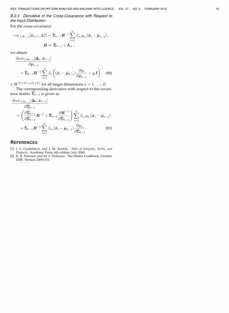
IEEE TRANSACTIONS ON PATTERN ANALYSIS AND MACHINE INTELLIGENCE, VOL. 37, NO. 2, FEBRUARY 2015 19
B.2.3 Derivative of the Cross-Covariance with Respect tothe Input DistributionFor the cross-covariance
covf,xt−1[xt−1,∆
at ] = Σt−1R
−1n∑i=1
βaiqai(xi − µt−1) ,
R := Σt−1 + Λa ,
we obtain∂covf,xt−1 [∆t, xt−1]
∂µt−1
= Σt−1R−1
n∑i=1
βi
((xi − µt−1)
∂qi∂µt−1
+ qiI
)(80)
∈ R(D+F )×(D+F ) for all target dimensions a = 1, . . . , E.The corresponding derivative with respect to the covari-
ance matrix Σt−1 is given as
∂covf,xt−1 [∆t, xt−1]
∂Σt−1
=
(∂Σt−1
∂Σt−1R−1 + Σt−1
∂R−1
∂Σt−1
)n∑i=1
βaiqai(xi − µt−1)
+ Σt−1R−1
n∑i=1
βai(xi − µt−1)∂qai∂Σt−1
. (81)
REFERENCES
[1] I. S. Gradshteyn and I. M. Ryzhik. Table of Integrals, Series, andProducts. Academic Press, 6th edition, July 2000.
[2] K. B. Petersen and M. S. Pedersen. The Matrix Cookbook, October2008. Version 20081110.