gaussian processes in python - university of...

Gaussian processes in python

John Reid

17th March 2009

1 What are Gaussian processes?

Often we have an inference problem involving n data,

D = {(xi, yi)|i = 1, . . . , n,xi ∈ X , yi ∈ R}

where the xi are the inputs and the yi are the targets. We wish to makepredictions, y∗, for new inputs x∗. Taking a Bayesian perspecitve we mightbuild a model that defines a distribution over all possible functions, f : X → R.We can encode our initial beliefs about our particular problem as a prior overthese functions. Given the data, D, and applying Bayes’ rule we can infera posterior distribution. In particular, for any given x∗ we can calculate orapproximate a predictive distribution over y∗ under this posterior.

Gaussian processes (GPs) are probability distributions over functions for whichthis inference task is tractable. They can be seen as a generalisation of theGaussian probability distribution to the space of functions. I.e. a multivariateGaussian distribution defines a distribution over a finite set of random variables,a Gaussian process defines a distribution over an infinite set of random variables,e.g. the real numbers. GP domains are not restricted to the real numbers, anyspace with a dot product is suitable. Analagously to a multivariate Gaussiandistribution, a GP is defined by its mean, µ, and covariance, k. However fora GP these are themselves functions, µ : X → R and k : X × X → R. In allthat follows we assume µ(x) = 0 without loss of generality as we can alwaysshift the data to accomodate any given mean. See figure 1 for samples from twoGaussian processes with X = R.

1.1 The covariance function, k

Assuming the mean function, µ, is 0 everywhere then our GP is defined by 2quantities, the data, If the mean is not 0 everywhere we can trivially shift thedata to make it so. D, and its covariance function (sometimes referred to as itskernel), k. The data is fixed so our modelling problem is exactly that of choosinga suitable covariance function. Given different problems we certainly wish tospecify different priors over possible functions. Fortunately we have available alarge library of possible covariance functions each of which represents a differentprior on the space of functions. See figure 2 for some examples.

1

Figure 1: Samples from 2 Gaussian processes with the same mean and covariancefunctions. The prior samples are taken from a Gaussian process without anydata and the posterior samples are taken from a Gaussian process where thedata are shown as black squares. The black dotted line represents the mean ofthe process and the gray shaded area covers twice the standard deviation at eachinput, x. The coloured lines are samples from the process, or more accuratelysamples at a finite number of inputs, x, joined by lines.

Furthermore the point-wise product and sum of covariance functions are them-selves covariance functions. In this way we can combine simple covariance func-tions to represent more complicated beliefs we have about our functions.

Normally we are modelling a system where we do not actually have access tothe target values, y, but only noisy versions of them, y+ ε. If we assume ε has aGaussian distribution with variance σ2

n we can incorporate this noise term intoour covariance function. This requires that our noisy GP’s covariance function,knoise(x1, x2) is aware of whether x1 and x2 are the same input.

knoise(x1, x2) = k(x1, x2) + δ(x1 = x2)σ2n

The effects of different noise levels can be seen in figure 3.

Most of the commonly used covariance functions are parameterised. These canbe fixed if we are confident in our understanding of the problem. Alterna-tively we can treat them as hyper-parameters in our Bayesian inference taskand optimise them through some technique such as maximum likelihood es-timation or conjugate gradient descent. Figure 4 shows how optimising thehyper-parameters can help us model the data more accurately.

2 Installation

2

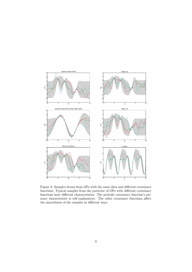
Figure 2: Samples drawn from GPs with the same data and different covariancefunctions. Typical samples from the posterior of GPs with different covariancefunctions have different characteristics. The periodic covariance function’s pri-mary characteristic is self explanatory. The other covariance functions affectthe smoothness of the samples in different ways.

3

Figure 3: GP predictions with varying levels of noise. The covariance functionis a squared exponential with additive noise of levels 0.0001, 0.1 and 1.

Figure 4: The effects of learning covariance function hyper-parameters. We seethe predictions in the figure on the right seem to fit the data more accurately.

4

3 Examples

We generate some test data using

import numpy, pylab, infpy.gp

# Generate some noisy data from a modulated sin curve

x_min, x_max = 10.0, 100.0X = infpy.gp.gp_1D_X_range(x_min, x_max) # input domain

Y = 10.0 * numpy.sin(X[:,0]) / X[:,0] # noise free output

Y = infpy.gp.gp_zero_mean(Y) # shift so mean=0.

e = 0.03 * numpy.random.normal(size = len(Y)) # noise

f = Y + e # noisy output

# a function to save plots

def save_fig(prefix):"Save current figure in extended postscript and PNG formats."pylab.savefig(’%s.png’ % prefix, format=’PNG’)pylab.savefig(’%s.eps’ % prefix, format=’EPS’)

# plot the noisy data

pylab.figure()pylab.plot(X[:,0], Y, ’b-’, label=’Y’)pylab.plot(X[:,0], f, ’rs’, label=’f’)pylab.legend()save_fig(’simple-example-data’)pylab.close()

The fs are noisy observations of the underlying Y s. How can we model thisusing GPs?

Using the following function as an interface to the infpy GP library,

5

def predict_values(K, file_tag, learn=False):"""

Create a GP with kernel K and predict values.

Optionally learn K’s hyperparameters if learn==True.

"""

gp = infpy.gp.GaussianProcess(X, f, K)if learn:infpy.gp.gp_learn_hyperparameters(gp)

pylab.figure()infpy.gp.gp_1D_predict(gp, 90, x_min - 10., x_max + 10.)save_fig(file_tag)pylab.close()

we can test various different kernels to see how well they fit the data. Forinstance a simple squared exponential kernel with some noise

# import short forms of GP kernel names

import infpy.gp.kernel_short_names as kernels

# create a kernel composed of a squared exponential kernel

# and a small noise term

K = kernels.SE() + kernels.Noise(.1)predict_values(K, ’simple-example-se’)

will generate

if we change the kernel so that the squared exponential term is given a shortercharacteristic length scale

# Try a different kernel with a shorter characteristic length scale

K = kernels.SE([.1]) + kernels.Noise(.1)predict_values(K, ’simple-example-se-shorter’)

6

we will generate

Here the shorter length scale means that data points are less correlated as theGP allows more variation over the same distance. The estimates of the noisebetween the training points is now much higher.

If we try a kernel with more noise

# Try another kernel with a lot more noise

K = kernels.SE([4.]) + kernels.Noise(1.)predict_values(K, ’simple-example-more-noise’)

we get the following estimates showing that the training data does not affectthe predictions as much

7

Perhaps we are really interested in learning the hyperparameters. We canacheive this as follows

# Try to learn kernel hyper-parameters

K = kernels.SE([4.0]) + kernels.Noise(.1)predict_values(K, ’simple-example-learnt’, learn=True)

and the result is

where the learnt length-scale is about 2.6 and the learnt noise level is about0.03.

4 Appendix A - Code for figures

We list the code that generated the figures in this document.

4.1 Code for figure 1

from numpy.random import seedfrom infpy.gp import GaussianProcess, gp_1D_X_range, gp_plot_samples_fromfrom pylab import plot, savefig, title, close, figure, xlabel, ylabel

# seed RNG to make reproducible and close all existing plot windows

seed(2)close(’all’)

#

# Kernel

#

from infpy.gp import SquaredExponentialKernel as SE

8

Figure 5: An application of GPs with periodic covariance functions to UK gasconsumption data. Top left : The data which has been shifted to have a meanof 0. Top right : A GP incorporating some noise and a fixed long length scalesquared exponential kernel. Bottom left : As top right but with a periodic term.Bottom right : As bottom left but with a periodic term with a reasonable period.

kernel = SE([1])

#

# Part of X-space we will plot samples from

#

support = gp_1D_X_range(-10.0, 10.01, .125)

#

# Plot samples from prior

#

figure()gp = GaussianProcess([], [], kernel)gp_plot_samples_from(gp, support, num_samples=3)xlabel(’x’)ylabel(’f(x)’)title(’Samples from the prior’)savefig(’samples_from_prior.png’)savefig(’samples_from_prior.eps’)

#

# Data

#

9

X = [[-5.], [-2.], [3.], [3.5]]Y = [2.5, 2, -.5, 0.]

#

# Plot samples from posterior

#

figure()plot([x[0] for x in X], Y, ’ks’)gp = GaussianProcess(X, Y, kernel)gp_plot_samples_from(gp, support, num_samples=3)xlabel(’x’)ylabel(’f(x)’)title(’Samples from the posterior’)savefig(’samples_from_posterior.png’)savefig(’samples_from_posterior.eps’)


from numpy.random import seedfrom infpy.gp import GaussianProcess, gp_1D_X_range, gp_plot_samples_fromfrom pylab import plot, savefig, title, close, figure, xlabel, ylabelfrom infpy.gp import SquaredExponentialKernel as SEfrom infpy.gp import Matern52Kernel as Matern52from infpy.gp import Matern52Kernel as Matern32from infpy.gp import RationalQuadraticKernel as RQfrom infpy.gp import NeuralNetworkKernel as NNfrom infpy.gp import FixedPeriod1DKernel as Periodicfrom infpy.gp import noise_kernel as noise

# seed RNG to make reproducible and close all existing plot windows

seed(2)close(’all’)

#

# Part of X-space we will plot samples from

#


#

# Data

#

X = [[-5.], [-2.], [3.], [3.5]]Y = [2.5, 2, -.5, 0.]

def plot_for_kernel(kernel, fig_title, filename):figure()plot([x[0] for x in X], Y, ’ks’)gp = GaussianProcess(X, Y, kernel)gp_plot_samples_from(gp, support, num_samples=3)

10

xlabel(’x’)ylabel(’f(x)’)title(fig_title)savefig(’%s.png’ % filename)savefig(’%s.eps’ % filename)

plot_for_kernel(kernel=Periodic(6.2),fig_title=’Periodic’,filename=’covariance_function_periodic’

)

plot_for_kernel(kernel=RQ(1., dimensions=1),fig_title=’Rational quadratic’,filename=’covariance_function_rq’

)

plot_for_kernel(kernel=SE([1]),fig_title=’Squared exponential’,filename=’covariance_function_se’

)

plot_for_kernel(kernel=SE([3.]),fig_title=’Squared exponential (long length scale)’,filename=’covariance_function_se_long_length’

)

plot_for_kernel(kernel=Matern52([1.]),fig_title=’Matern52’,filename=’covariance_function_matern_52’

)

plot_for_kernel(kernel=Matern32([1.]),fig_title=’Matern32’,filename=’covariance_function_matern_32’

)


from numpy.random import seedfrom infpy.gp import GaussianProcess, gp_1D_X_range, gp_plot_predictionfrom pylab import plot, savefig, title, close, figure, xlabel, ylabelfrom infpy.gp import SquaredExponentialKernel as SEfrom infpy.gp import noise_kernel as noise

11

# close all existing plot windows

close(’all’)

#

# Part of X-space we are interested in

#


#

# Data

#

X = [[-5.], [-2.], [3.], [3.5]]Y = [2.5, 2, -.5, 0.]

def plot_for_kernel(kernel, fig_title, filename):figure()plot([x[0] for x in X], Y, ’ks’)gp = GaussianProcess(X, Y, kernel)mean, sigma, LL = gp.predict(support)gp_plot_prediction(support, mean, sigma)xlabel(’x’)ylabel(’f(x)’)title(fig_title)savefig(’%s.png’ % filename)savefig(’%s.eps’ % filename)

plot_for_kernel(kernel=SE([1.]) + noise(.1),fig_title=’k = SE + noise(.1)’,filename=’noise_mid’

)

plot_for_kernel(kernel=SE([1.]) + noise(1.),fig_title=’k = SE + noise(1)’,filename=’noise_high’

)

plot_for_kernel(kernel=SE([1.]) + noise(.0001),fig_title=’k = SE + noise(.0001)’,filename=’noise_low’

)


from numpy.random import seedfrom infpy.gp import GaussianProcess, gp_1D_X_range

12

from infpy.gp import gp_plot_prediction, gp_learn_hyperparametersfrom pylab import plot, savefig, title, close, figure, xlabel, ylabelfrom infpy.gp import SquaredExponentialKernel as SEfrom infpy.gp import noise_kernel as noise

# close all existing plot windows

close(’all’)

#

# Part of X-space we are interested in

#


#

# Data

#

X = [[-5.], [-2.], [3.], [3.5]]Y = [2.5, 2, -.5, 0.]

def plot_gp(gp, fig_title, filename):figure()plot([x[0] for x in X], Y, ’ks’)mean, sigma, LL = gp.predict(support)gp_plot_prediction(support, mean, sigma)xlabel(’x’)ylabel(’f(x)’)title(fig_title)savefig(’%s.png’ % filename)savefig(’%s.eps’ % filename)

#

# Create a kernel with reasonable parameters and plot the GP predictions

#

kernel = SE([1.]) + noise(1.)gp = GaussianProcess(X, Y, kernel)plot_gp(gp=gp,fig_title=’Initial parameters: kernel = SE([1]) + noise(1)’,filename=’learning_first_guess’

)

#

# Learn the covariance function’s parameters and replot

#

gp_learn_hyperparameters(gp)plot_gp(gp=gp,fig_title=’Learnt parameters: kernel = SE([%.2f]) + noise(%.2f)’ % (kernel.k1.params[0],kernel.k2.params.o2[0]

13

),filename=’learning_learnt’

)

14

Figure 6: Modulated sine example: Top left : The data: a modulated noisy sinewave. Top right : GP with a squared exponential kernel. Middle left : GP witha squared exponential kernel with a shorter length scale. Middle right : GPwith a squared exponential kernel with a larger noise term. Bottom: GP witha squared exponential kernel with learnt hyper-parameters.

15

gaussian processes in python - university of...

Documents