gaussian processes: the next step in exoplanet data …mosb/public/pdf/2053/algrain...gaussian...
TRANSCRIPT
Gaussian processes: the next step in exoplanet data analysis
Suzanne Aigrain (University of Oxford) Neale Gibson, Tom Evans, Amy McQuillan
Steve Roberts, Steve Reece, Mike Osborne
... let the data speak

Gaussian processes: the next step in exoplanet data analysis
Suzanne Aigrain (University of Oxford) Neale Gibson, Tom Evans, Amy McQuillan
Steve Roberts, Steve Reece, Mike OsborneGaussian processes for modelling systematics 5
Figure 1. The ‘raw’ HD 189733 NICMOS dataset used as an example for our Gaussian process model. Left: Raw light curves of HD189733 for each of the 18 wavelength channels, from 2.50µm to 1.48µm top to bottom. Right: The optical state parameters extractedfrom the spectra plotted as a time series. These are used as the input parameters for our GP model. The red lines represent a GPregression on the input parameters, used to remove the noise and test how this effects the GP model.
the noisy input parameters. We also checked that the choice
of hyperprior length scale had little effect on the results, by
setting them to large values, and repeating the procedure
with varying length scales ensuring the transmission spec-
tra were not significantly altered.
3.2 Type-II maximum likelihood
As mentioned in Sect. 2.4, a useful approximation is Type-II
maximum likelihood. First, the log posterior is maximised
with respect to the hyperparameters and variable mean-
function parameters using a Nelder-Mead simplex algorithm
(see e.g. Press et al. 1992). The transit model is the same
as that used in GPA11, which uses Mandel & Agol (2002)
models calculated assuming quadratic limb darkening and a
circular orbit. All non-variable parameters were fixed to the
values given in Pont et al. (2008), except for the limb dark-
ening parameters, which were calculated for each wavelength
channel (GPA11, Sing 2010). The only variable mean func-
tion variable parameters are the planet-to-star radius ratio,
and two parameters that govern a linear baseline model; an
out-of-transit flux foot and (time) gradient Tgrad.
An example of the predictive distributions found using
type-II maximum likelihood is shown in Fig. 2 for four of the
wavelength channels. In this example, only orbits 2, 3 and 5
are used to determine the parameters and hyperparameters
of the GP (or ‘train’ the GP), and are shown by the red
points4. Orbit 4 (green points) was not used in the training
set. Predictive distributions were calculated for orbits 2–5,
and are shown by the grey regions, which plot the 1 and 2σconfidence intervals. The predictive distribution is a good fit
to orbit 4, showing that our GP model is effective at mod-
elling the instrumental systematics. The systematics model
will of course be even more constrained than in this exam-
ple, as we use orbits 2–5 to simultaneously infer parameters
of the GP and transit function.
Now that all parameters and hyperparameters are opti-
mised with respect to the posterior distribution, the hyper-
parameters are held fixed. This means the inverse covari-
ance matrix and log determinant used to evaluate the log
posterior are also fixed, and need calculated only once. An
MCMC is used to marginalise over the remaining parame-
ters of interest, in this case the planet-to-star radius ratio
4 We used the smoothed hyperparameters here for aesthetic pur-poses. Using the noisy hyperparameters would simply result innoisy predictive distributions.
c� 2002 RAS, MNRAS 000, 1–12
time-seriescorrelated
disentangle
high precision
noise
stoch
astic
... let the data speak

A Gaussian process in a nutshell
2 N. P. Gibson, S. Aigrain et al.
GAUSSIAN PROCESSES FOR REGRESSION
Models based on Gaussian processes are extensively used inthe machine learning community for Bayesian inference inregression and classification problems. They can be seen asan extension of kernel regression to probabilistic models. Inthis appendix, we endeavour to give a very brief introductionto the use of GPs for regression. Our explanations are basedon the textbooks by Rassmussen & Williams (2006) andBishop (2006), where the interested reader will find far morecomplete and detailed information.
Introducing Gaussian processes
Consider a collection of N observations, each consisting ofD known inputs, or independent variables, and one output,or dependent variable, which is measured with finite accu-racy (it is trival to extend the same reasoning to more thanone, jointly observed outputs). In the case of observationsof a planetary transit in a single bandpass, for example, theoutput is a flux or magnitude, and the inputs might includethe time at which the observations were made, but also an-cillary data pertaining to the state of the instrument andthe observing conditions. In the machine learning literature,observed outputs are usually referred to as targets, becausethe quality of a model is measured by its ability to repro-duce the targets, given the inputs, and we shall adopt thisconvention here.
We write the inputs for the nth observation as a columnvector xn = (x1,n . . . , xD,n)T, and the corresponding targetvalue as tn. The N target values are then collated into acolumn vector t = (t1, . . . , tN )T, and the D×N outputs intoa matrix X, with elements Xij = xi,j . A standard approach,which most astronomers will be familiar with, is to modelthe data as:
t = m(X, φ) + �
where m is a mean function with parameters φ, which actson the matrix of N input vectors, returning an N -elementvector, and � represents independent, identically distributed(i.i.d.) noise
� ∼ N�0, σ2I
�.
Here N [a,B] represents a multivariate Gaussian distribu-tion with mean vector a and covariance matrix B, σ is thestandard deviation of the noise, and I is the identity matrix.The joint probability distribution for a set of outputs t isthus:
P (t |X, σ, φ) = N�m(X, φ), σ2I
�
A Gaussian process (hereafter GP) is defined by the factthat the joint distribution of any set of samples drawn from aGP is a multivariate Gaussian distribution. Therefore, i.i.d.noise is a special case of GP. We now extend our model tothe general GP case:
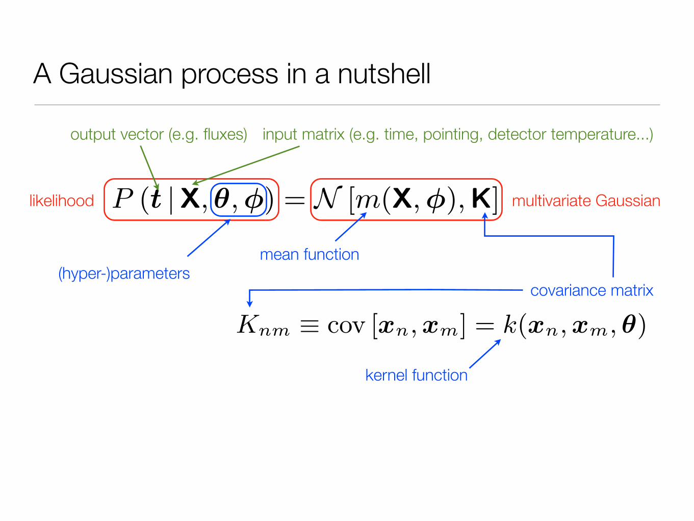
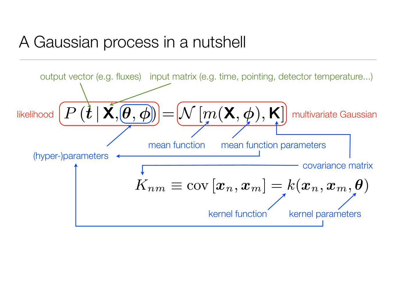
P (t |X, θ, φ) = N [m(X, φ),K] (1)
where the covariance matrix K has elements
Knm ≡ cov [xn, xm] = k(xn, xm, θ)
The function k, known as the covariance function or kernel,has parameters θ, and acts on a pair of inputs, returning the
covariance between the corresponding outputs. The specifi-cation of the covariance function implies a probability dis-tribution over functions, and we can draw samples from thisdistribution by choosing a number of input points, writingout the corresponding covariance matrix, and generating arandom Gaussian vector with this covariance matrix. Insert
reference to figure.
The mean function controls the deterministic compo-nent of the model, whilst the covariance function controlsits stochastic component. Depending on the situation, theformer may simply be zero everywhere. Similarly, the lattermay represent a physical process of interest, or it may repre-sent noise. A commonly used family of covariance functionsis the squared exponential kernel:
kSE(xn, xm, θ) = θ0 exp
�θ1
D�
i=1
(xi,n − xi,m)2
�
where θ0 is an amplitude, and θ1 an inverse length scale(this becomes more obvious if we write θ1 = 1/2l2). Pairs ofobservations generated from the squared exponential kernelare strongly mutually correlated if they lie near each other ininput space, and relatively uncorrelated if they are mutuallydistant in input space. Multiple covariance functions can beadded or multipled together to model multiple stochasticprocesses simultaneously occurring in the data. For example,most GP models include an i.i.d. component:
k(xn, xm, θ, σ) = kSE(xn, xm, θ) + δnmσ2
where δ is the Kronecker delta function.The joint probability given by equation 1 is the likeli-
hood of observing the targets t, given X, φ and θ. This likeli-hood is already marginalised over all possible realisations ofthe stochastic component, which satisfy the covariance ma-trix specified by X and θ. In this sense, GPs are intrinsicallyBayesian. In fact, one can show that GP regression with thesquared exponential kernel is equivalent to Bayesian linearregression with an infinite number of basis functions1. Thebasis function weights can be seen as the parameters of themodel, and in Bayesian jargon, the elements of θ and φ areall hyper-parameters of the model.
GPs as interpolation tools
Given a set of inputs X and observed targets t, we may wishto make predictions for a new set of inputs X�. We refer
1 In the Bayesian linear basis equivalent of GP regression, thebasis function weights are subject to an automatic relevance de-termination (ARD) priors. These priors are zero-mean Gaussians,which force the weights to be zero unless there is evidence in thedata to support a non-zero value. This helps to explain how GPscan be extremely flexible, yet avoid the over-fitting problem whichaffects maximum-likelihood linear models. In linear basis mod-elling, one seeks a global probability maximum in feature space,where each coordinate represents the weight of a particular ba-sis function. Working with a high-dimensional feature space isproblematic: it gives rise to degeneracy, numerical instability andexcessive computational demand. This problem is known as thecurse of dimensionality. GPs belong to a class of methods, whichcircumvent this problem by working in function space rather thanfeature space, and parametrising the functions in terms of theircovariance properties. This is known as the kernel trick.
c� 2011 RAS, MNRAS 000, 1–??

A Gaussian process in a nutshell
2 N. P. Gibson, S. Aigrain et al.
GAUSSIAN PROCESSES FOR REGRESSION
Models based on Gaussian processes are extensively used inthe machine learning community for Bayesian inference inregression and classification problems. They can be seen asan extension of kernel regression to probabilistic models. Inthis appendix, we endeavour to give a very brief introductionto the use of GPs for regression. Our explanations are basedon the textbooks by Rassmussen & Williams (2006) andBishop (2006), where the interested reader will find far morecomplete and detailed information.
Introducing Gaussian processes
Consider a collection of N observations, each consisting ofD known inputs, or independent variables, and one output,or dependent variable, which is measured with finite accu-racy (it is trival to extend the same reasoning to more thanone, jointly observed outputs). In the case of observationsof a planetary transit in a single bandpass, for example, theoutput is a flux or magnitude, and the inputs might includethe time at which the observations were made, but also an-cillary data pertaining to the state of the instrument andthe observing conditions. In the machine learning literature,observed outputs are usually referred to as targets, becausethe quality of a model is measured by its ability to repro-duce the targets, given the inputs, and we shall adopt thisconvention here.
We write the inputs for the nth observation as a columnvector xn = (x1,n . . . , xD,n)T, and the corresponding targetvalue as tn. The N target values are then collated into acolumn vector t = (t1, . . . , tN )T, and the D×N outputs intoa matrix X, with elements Xij = xi,j . A standard approach,which most astronomers will be familiar with, is to modelthe data as:
t = m(X, φ) + �
where m is a mean function with parameters φ, which actson the matrix of N input vectors, returning an N -elementvector, and � represents independent, identically distributed(i.i.d.) noise
� ∼ N�0, σ2I
�.
Here N [a,B] represents a multivariate Gaussian distribu-tion with mean vector a and covariance matrix B, σ is thestandard deviation of the noise, and I is the identity matrix.The joint probability distribution for a set of outputs t isthus:
P (t |X, σ, φ) = N�m(X, φ), σ2I
�
A Gaussian process (hereafter GP) is defined by the factthat the joint distribution of any set of samples drawn from aGP is a multivariate Gaussian distribution. Therefore, i.i.d.noise is a special case of GP. We now extend our model tothe general GP case:
P (t |X, θ, φ) = N [m(X, φ),K] (1)
where the covariance matrix K has elements
Knm ≡ cov [xn, xm] = k(xn, xm, θ)
The function k, known as the covariance function or kernel,has parameters θ, and acts on a pair of inputs, returning the
covariance between the corresponding outputs. The specifi-cation of the covariance function implies a probability dis-tribution over functions, and we can draw samples from thisdistribution by choosing a number of input points, writingout the corresponding covariance matrix, and generating arandom Gaussian vector with this covariance matrix. Insert
reference to figure.
The mean function controls the deterministic compo-nent of the model, whilst the covariance function controlsits stochastic component. Depending on the situation, theformer may simply be zero everywhere. Similarly, the lattermay represent a physical process of interest, or it may repre-sent noise. A commonly used family of covariance functionsis the squared exponential kernel:
kSE(xn, xm, θ) = θ0 exp
�θ1
D�
i=1
(xi,n − xi,m)2
�
where θ0 is an amplitude, and θ1 an inverse length scale(this becomes more obvious if we write θ1 = 1/2l2). Pairs ofobservations generated from the squared exponential kernelare strongly mutually correlated if they lie near each other ininput space, and relatively uncorrelated if they are mutuallydistant in input space. Multiple covariance functions can beadded or multipled together to model multiple stochasticprocesses simultaneously occurring in the data. For example,most GP models include an i.i.d. component:
k(xn, xm, θ, σ) = kSE(xn, xm, θ) + δnmσ2
where δ is the Kronecker delta function.The joint probability given by equation 1 is the likeli-
hood of observing the targets t, given X, φ and θ. This likeli-hood is already marginalised over all possible realisations ofthe stochastic component, which satisfy the covariance ma-trix specified by X and θ. In this sense, GPs are intrinsicallyBayesian. In fact, one can show that GP regression with thesquared exponential kernel is equivalent to Bayesian linearregression with an infinite number of basis functions1. Thebasis function weights can be seen as the parameters of themodel, and in Bayesian jargon, the elements of θ and φ areall hyper-parameters of the model.
GPs as interpolation tools
Given a set of inputs X and observed targets t, we may wishto make predictions for a new set of inputs X�. We refer
1 In the Bayesian linear basis equivalent of GP regression, thebasis function weights are subject to an automatic relevance de-termination (ARD) priors. These priors are zero-mean Gaussians,which force the weights to be zero unless there is evidence in thedata to support a non-zero value. This helps to explain how GPscan be extremely flexible, yet avoid the over-fitting problem whichaffects maximum-likelihood linear models. In linear basis mod-elling, one seeks a global probability maximum in feature space,where each coordinate represents the weight of a particular ba-sis function. Working with a high-dimensional feature space isproblematic: it gives rise to degeneracy, numerical instability andexcessive computational demand. This problem is known as thecurse of dimensionality. GPs belong to a class of methods, whichcircumvent this problem by working in function space rather thanfeature space, and parametrising the functions in terms of theircovariance properties. This is known as the kernel trick.
c� 2011 RAS, MNRAS 000, 1–??
likelihood
output vector (e.g. fluxes) input matrix (e.g. time, pointing, detector temperature...)
(hyper-)parameters

A Gaussian process in a nutshell
2 N. P. Gibson, S. Aigrain et al.
GAUSSIAN PROCESSES FOR REGRESSION
Models based on Gaussian processes are extensively used inthe machine learning community for Bayesian inference inregression and classification problems. They can be seen asan extension of kernel regression to probabilistic models. Inthis appendix, we endeavour to give a very brief introductionto the use of GPs for regression. Our explanations are basedon the textbooks by Rassmussen & Williams (2006) andBishop (2006), where the interested reader will find far morecomplete and detailed information.
Introducing Gaussian processes
Consider a collection of N observations, each consisting ofD known inputs, or independent variables, and one output,or dependent variable, which is measured with finite accu-racy (it is trival to extend the same reasoning to more thanone, jointly observed outputs). In the case of observationsof a planetary transit in a single bandpass, for example, theoutput is a flux or magnitude, and the inputs might includethe time at which the observations were made, but also an-cillary data pertaining to the state of the instrument andthe observing conditions. In the machine learning literature,observed outputs are usually referred to as targets, becausethe quality of a model is measured by its ability to repro-duce the targets, given the inputs, and we shall adopt thisconvention here.
We write the inputs for the nth observation as a columnvector xn = (x1,n . . . , xD,n)T, and the corresponding targetvalue as tn. The N target values are then collated into acolumn vector t = (t1, . . . , tN )T, and the D×N outputs intoa matrix X, with elements Xij = xi,j . A standard approach,which most astronomers will be familiar with, is to modelthe data as:
t = m(X, φ) + �
where m is a mean function with parameters φ, which actson the matrix of N input vectors, returning an N -elementvector, and � represents independent, identically distributed(i.i.d.) noise
� ∼ N�0, σ2I
�.
Here N [a,B] represents a multivariate Gaussian distribu-tion with mean vector a and covariance matrix B, σ is thestandard deviation of the noise, and I is the identity matrix.The joint probability distribution for a set of outputs t isthus:
P (t |X, σ, φ) = N�m(X, φ), σ2I
�
A Gaussian process (hereafter GP) is defined by the factthat the joint distribution of any set of samples drawn from aGP is a multivariate Gaussian distribution. Therefore, i.i.d.noise is a special case of GP. We now extend our model tothe general GP case:
P (t |X, θ, φ) = N [m(X, φ),K] (1)
where the covariance matrix K has elements
Knm ≡ cov [xn, xm] = k(xn, xm, θ)
The function k, known as the covariance function or kernel,has parameters θ, and acts on a pair of inputs, returning the
covariance between the corresponding outputs. The specifi-cation of the covariance function implies a probability dis-tribution over functions, and we can draw samples from thisdistribution by choosing a number of input points, writingout the corresponding covariance matrix, and generating arandom Gaussian vector with this covariance matrix. Insert
reference to figure.
The mean function controls the deterministic compo-nent of the model, whilst the covariance function controlsits stochastic component. Depending on the situation, theformer may simply be zero everywhere. Similarly, the lattermay represent a physical process of interest, or it may repre-sent noise. A commonly used family of covariance functionsis the squared exponential kernel:
kSE(xn, xm, θ) = θ0 exp
�θ1
D�
i=1
(xi,n − xi,m)2
�
where θ0 is an amplitude, and θ1 an inverse length scale(this becomes more obvious if we write θ1 = 1/2l2). Pairs ofobservations generated from the squared exponential kernelare strongly mutually correlated if they lie near each other ininput space, and relatively uncorrelated if they are mutuallydistant in input space. Multiple covariance functions can beadded or multipled together to model multiple stochasticprocesses simultaneously occurring in the data. For example,most GP models include an i.i.d. component:
k(xn, xm, θ, σ) = kSE(xn, xm, θ) + δnmσ2
where δ is the Kronecker delta function.The joint probability given by equation 1 is the likeli-
hood of observing the targets t, given X, φ and θ. This likeli-hood is already marginalised over all possible realisations ofthe stochastic component, which satisfy the covariance ma-trix specified by X and θ. In this sense, GPs are intrinsicallyBayesian. In fact, one can show that GP regression with thesquared exponential kernel is equivalent to Bayesian linearregression with an infinite number of basis functions1. Thebasis function weights can be seen as the parameters of themodel, and in Bayesian jargon, the elements of θ and φ areall hyper-parameters of the model.
GPs as interpolation tools
Given a set of inputs X and observed targets t, we may wishto make predictions for a new set of inputs X�. We refer
1 In the Bayesian linear basis equivalent of GP regression, thebasis function weights are subject to an automatic relevance de-termination (ARD) priors. These priors are zero-mean Gaussians,which force the weights to be zero unless there is evidence in thedata to support a non-zero value. This helps to explain how GPscan be extremely flexible, yet avoid the over-fitting problem whichaffects maximum-likelihood linear models. In linear basis mod-elling, one seeks a global probability maximum in feature space,where each coordinate represents the weight of a particular ba-sis function. Working with a high-dimensional feature space isproblematic: it gives rise to degeneracy, numerical instability andexcessive computational demand. This problem is known as thecurse of dimensionality. GPs belong to a class of methods, whichcircumvent this problem by working in function space rather thanfeature space, and parametrising the functions in terms of theircovariance properties. This is known as the kernel trick.
c� 2011 RAS, MNRAS 000, 1–??
multivariate Gaussian
mean function
covariance matrix
likelihood
output vector (e.g. fluxes) input matrix (e.g. time, pointing, detector temperature...)
(hyper-)parameters
A Gaussian process in a nutshell
2 N. P. Gibson, S. Aigrain et al.
GAUSSIAN PROCESSES FOR REGRESSION
Models based on Gaussian processes are extensively used inthe machine learning community for Bayesian inference inregression and classification problems. They can be seen asan extension of kernel regression to probabilistic models. Inthis appendix, we endeavour to give a very brief introductionto the use of GPs for regression. Our explanations are basedon the textbooks by Rassmussen & Williams (2006) andBishop (2006), where the interested reader will find far morecomplete and detailed information.
Introducing Gaussian processes
Consider a collection of N observations, each consisting ofD known inputs, or independent variables, and one output,or dependent variable, which is measured with finite accu-racy (it is trival to extend the same reasoning to more thanone, jointly observed outputs). In the case of observationsof a planetary transit in a single bandpass, for example, theoutput is a flux or magnitude, and the inputs might includethe time at which the observations were made, but also an-cillary data pertaining to the state of the instrument andthe observing conditions. In the machine learning literature,observed outputs are usually referred to as targets, becausethe quality of a model is measured by its ability to repro-duce the targets, given the inputs, and we shall adopt thisconvention here.
We write the inputs for the nth observation as a columnvector xn = (x1,n . . . , xD,n)T, and the corresponding targetvalue as tn. The N target values are then collated into acolumn vector t = (t1, . . . , tN )T, and the D×N outputs intoa matrix X, with elements Xij = xi,j . A standard approach,which most astronomers will be familiar with, is to modelthe data as:
t = m(X, φ) + �
where m is a mean function with parameters φ, which actson the matrix of N input vectors, returning an N -elementvector, and � represents independent, identically distributed(i.i.d.) noise
� ∼ N�0, σ2I
�.
Here N [a,B] represents a multivariate Gaussian distribu-tion with mean vector a and covariance matrix B, σ is thestandard deviation of the noise, and I is the identity matrix.The joint probability distribution for a set of outputs t isthus:
P (t |X, σ, φ) = N�m(X, φ), σ2I
�
A Gaussian process (hereafter GP) is defined by the factthat the joint distribution of any set of samples drawn from aGP is a multivariate Gaussian distribution. Therefore, i.i.d.noise is a special case of GP. We now extend our model tothe general GP case:
P (t |X, θ, φ) = N [m(X, φ),K] (1)
where the covariance matrix K has elements
Knm ≡ cov [xn, xm] = k(xn, xm, θ)
The function k, known as the covariance function or kernel,has parameters θ, and acts on a pair of inputs, returning the
covariance between the corresponding outputs. The specifi-cation of the covariance function implies a probability dis-tribution over functions, and we can draw samples from thisdistribution by choosing a number of input points, writingout the corresponding covariance matrix, and generating arandom Gaussian vector with this covariance matrix. Insert
reference to figure.
The mean function controls the deterministic compo-nent of the model, whilst the covariance function controlsits stochastic component. Depending on the situation, theformer may simply be zero everywhere. Similarly, the lattermay represent a physical process of interest, or it may repre-sent noise. A commonly used family of covariance functionsis the squared exponential kernel:
kSE(xn, xm, θ) = θ0 exp
�θ1
D�
i=1
(xi,n − xi,m)2
�
where θ0 is an amplitude, and θ1 an inverse length scale(this becomes more obvious if we write θ1 = 1/2l2). Pairs ofobservations generated from the squared exponential kernelare strongly mutually correlated if they lie near each other ininput space, and relatively uncorrelated if they are mutuallydistant in input space. Multiple covariance functions can beadded or multipled together to model multiple stochasticprocesses simultaneously occurring in the data. For example,most GP models include an i.i.d. component:
k(xn, xm, θ, σ) = kSE(xn, xm, θ) + δnmσ2
where δ is the Kronecker delta function.The joint probability given by equation 1 is the likeli-
hood of observing the targets t, given X, φ and θ. This likeli-hood is already marginalised over all possible realisations ofthe stochastic component, which satisfy the covariance ma-trix specified by X and θ. In this sense, GPs are intrinsicallyBayesian. In fact, one can show that GP regression with thesquared exponential kernel is equivalent to Bayesian linearregression with an infinite number of basis functions1. Thebasis function weights can be seen as the parameters of themodel, and in Bayesian jargon, the elements of θ and φ areall hyper-parameters of the model.
GPs as interpolation tools
Given a set of inputs X and observed targets t, we may wishto make predictions for a new set of inputs X�. We refer
1 In the Bayesian linear basis equivalent of GP regression, thebasis function weights are subject to an automatic relevance de-termination (ARD) priors. These priors are zero-mean Gaussians,which force the weights to be zero unless there is evidence in thedata to support a non-zero value. This helps to explain how GPscan be extremely flexible, yet avoid the over-fitting problem whichaffects maximum-likelihood linear models. In linear basis mod-elling, one seeks a global probability maximum in feature space,where each coordinate represents the weight of a particular ba-sis function. Working with a high-dimensional feature space isproblematic: it gives rise to degeneracy, numerical instability andexcessive computational demand. This problem is known as thecurse of dimensionality. GPs belong to a class of methods, whichcircumvent this problem by working in function space rather thanfeature space, and parametrising the functions in terms of theircovariance properties. This is known as the kernel trick.
c� 2011 RAS, MNRAS 000, 1–??
multivariate Gaussian
mean function
covariance matrix
2 N. P. Gibson, S. Aigrain et al.
GAUSSIAN PROCESSES FOR REGRESSION
Models based on Gaussian processes are extensively used inthe machine learning community for Bayesian inference inregression and classification problems. They can be seen asan extension of kernel regression to probabilistic models. Inthis appendix, we endeavour to give a very brief introductionto the use of GPs for regression. Our explanations are basedon the textbooks by Rassmussen & Williams (2006) andBishop (2006), where the interested reader will find far morecomplete and detailed information.
Introducing Gaussian processes
Consider a collection of N observations, each consisting ofD known inputs, or independent variables, and one output,or dependent variable, which is measured with finite accu-racy (it is trival to extend the same reasoning to more thanone, jointly observed outputs). In the case of observationsof a planetary transit in a single bandpass, for example, theoutput is a flux or magnitude, and the inputs might includethe time at which the observations were made, but also an-cillary data pertaining to the state of the instrument andthe observing conditions. In the machine learning literature,observed outputs are usually referred to as targets, becausethe quality of a model is measured by its ability to repro-duce the targets, given the inputs, and we shall adopt thisconvention here.
We write the inputs for the nth observation as a columnvector xn = (x1,n . . . , xD,n)T, and the corresponding targetvalue as tn. The N target values are then collated into acolumn vector t = (t1, . . . , tN )T, and the D×N outputs intoa matrix X, with elements Xij = xi,j . A standard approach,which most astronomers will be familiar with, is to modelthe data as:
t = m(X, φ) + �
where m is a mean function with parameters φ, which actson the matrix of N input vectors, returning an N -elementvector, and � represents independent, identically distributed(i.i.d.) noise
� ∼ N�0, σ2I
�.
Here N [a,B] represents a multivariate Gaussian distribu-tion with mean vector a and covariance matrix B, σ is thestandard deviation of the noise, and I is the identity matrix.The joint probability distribution for a set of outputs t isthus:
P (t |X, σ, φ) = N�m(X, φ), σ2I
�
A Gaussian process (hereafter GP) is defined by the factthat the joint distribution of any set of samples drawn from aGP is a multivariate Gaussian distribution. Therefore, i.i.d.noise is a special case of GP. We now extend our model tothe general GP case:
P (t |X, θ, φ) = N [m(X, φ),K] (1)
where the covariance matrix K has elements
Knm ≡ cov [xn, xm] = k(xn, xm, θ)
The function k, known as the covariance function or kernel,has parameters θ, and acts on a pair of inputs, returning the
covariance between the corresponding outputs. The specifi-cation of the covariance function implies a probability dis-tribution over functions, and we can draw samples from thisdistribution by choosing a number of input points, writingout the corresponding covariance matrix, and generating arandom Gaussian vector with this covariance matrix. Insert
reference to figure.
The mean function controls the deterministic compo-nent of the model, whilst the covariance function controlsits stochastic component. Depending on the situation, theformer may simply be zero everywhere. Similarly, the lattermay represent a physical process of interest, or it may repre-sent noise. A commonly used family of covariance functionsis the squared exponential kernel:
kSE(xn, xm, θ) = θ0 exp
�θ1
D�
i=1
(xi,n − xi,m)2
�
where θ0 is an amplitude, and θ1 an inverse length scale(this becomes more obvious if we write θ1 = 1/2l2). Pairs ofobservations generated from the squared exponential kernelare strongly mutually correlated if they lie near each other ininput space, and relatively uncorrelated if they are mutuallydistant in input space. Multiple covariance functions can beadded or multipled together to model multiple stochasticprocesses simultaneously occurring in the data. For example,most GP models include an i.i.d. component:
k(xn, xm, θ, σ) = kSE(xn, xm, θ) + δnmσ2
where δ is the Kronecker delta function.The joint probability given by equation 1 is the likeli-
hood of observing the targets t, given X, φ and θ. This likeli-hood is already marginalised over all possible realisations ofthe stochastic component, which satisfy the covariance ma-trix specified by X and θ. In this sense, GPs are intrinsicallyBayesian. In fact, one can show that GP regression with thesquared exponential kernel is equivalent to Bayesian linearregression with an infinite number of basis functions1. Thebasis function weights can be seen as the parameters of themodel, and in Bayesian jargon, the elements of θ and φ areall hyper-parameters of the model.
GPs as interpolation tools
Given a set of inputs X and observed targets t, we may wishto make predictions for a new set of inputs X�. We refer
1 In the Bayesian linear basis equivalent of GP regression, thebasis function weights are subject to an automatic relevance de-termination (ARD) priors. These priors are zero-mean Gaussians,which force the weights to be zero unless there is evidence in thedata to support a non-zero value. This helps to explain how GPscan be extremely flexible, yet avoid the over-fitting problem whichaffects maximum-likelihood linear models. In linear basis mod-elling, one seeks a global probability maximum in feature space,where each coordinate represents the weight of a particular ba-sis function. Working with a high-dimensional feature space isproblematic: it gives rise to degeneracy, numerical instability andexcessive computational demand. This problem is known as thecurse of dimensionality. GPs belong to a class of methods, whichcircumvent this problem by working in function space rather thanfeature space, and parametrising the functions in terms of theircovariance properties. This is known as the kernel trick.
c� 2011 RAS, MNRAS 000, 1–??
kernel function
likelihood
output vector (e.g. fluxes) input matrix (e.g. time, pointing, detector temperature...)
(hyper-)parameters
kernel parameters
mean function parameters
Gaussian process regression

Gaussian process regression
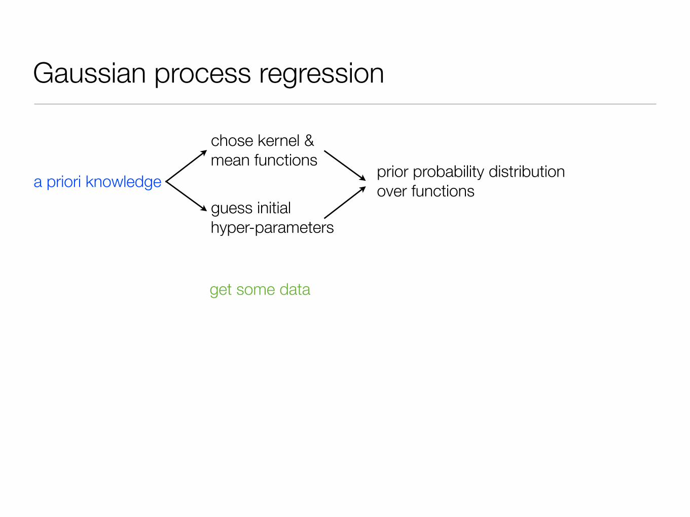
a priori knowledge

Gaussian process regression
a priori knowledge
chose kernel & mean functions
guess initial hyper-parameters

Gaussian process regression
a priori knowledge
chose kernel & mean functions
guess initial hyper-parameters
prior probability distribution over functions
Gaussian process regression
a priori knowledge
get some data
chose kernel & mean functions
guess initial hyper-parameters
prior probability distribution over functions

Gaussian process regression
a priori knowledge
get some data
chose kernel & mean functions
guess initial hyper-parameters
prior probability distribution over functions
condition the GP

Gaussian process regression
a priori knowledge
get some data
chose kernel & mean functions
guess initial hyper-parameters
prior probability distribution over functions
condition the GP
predictive (posterior)distribution

Gaussian process regression
a priori knowledge
get some data
chose kernel & mean functions
guess initial hyper-parameters
prior probability distribution over functions
condition the GP
predictive (posterior)distributionmarginal likelihood

Gaussian process regression
a priori knowledge
get some data
chose kernel & mean functions
guess initial hyper-parameters
prior probability distribution over functions
condition the GP
predictive (posterior)distributionmarginal likelihood
posterior distribution over hyper-parameters

Gaussian process regression
a priori knowledge
get some data
chose kernel & mean functions
guess initial hyper-parameters
prior probability distribution over functions
condition the GP
predictive (posterior)distribution
interpolate (predict)
marginal likelihoodposterior distribution over hyper-parameters

A very simple example12 N. P. Gibson et al.
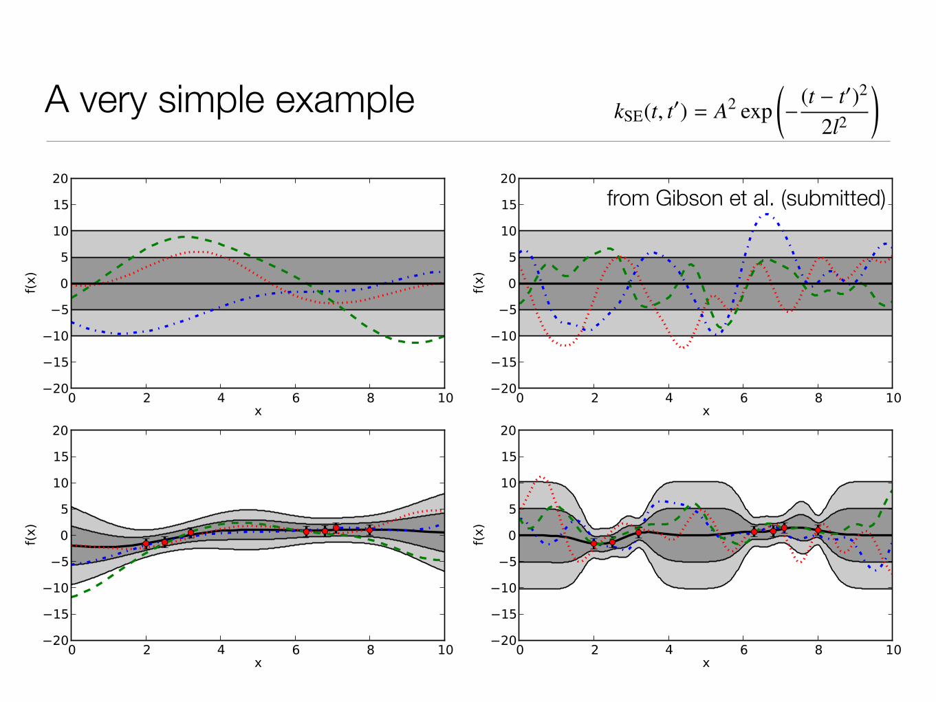
Figure A1. Top: Examples of random functions drawn from a GP with a squared exponential covariance kernel. The left and right plotshave hyperparameters {θ0, θ1} = {25, 2}, and {θ0, θ1} = {25, 0.5}, respectively. The dark and light grey shaded areas represent the 1and 2 σ boundaries of the distribution. Bottom: The predictive distributions generated after adding some training data and conditioningusing the same hyperparameters as the corresponding plots above, with the addition of a white noise term (σ2 = 1). The coloured linesare now random vectors drawn from the posterior distribution.
type-II maximum likelihood. This involves fixing the covari-
ance hyperparameters at their maximum likelihood values,
and marginalising over the remaining mean function hyper-
parameters of interest. This is a valid approximation when
the posterior distribution is sharply peaked at its maximum
with respect to the covariance hyperparameters, and should
give similar results to the full marginalisation.
Fig. A2 gives examples of GP regression using a squared
exponential covariance function, after optimising the hyper-
parameters via a Nelder-Mead simplex algorithm (see e.g.
Press et al. 1992). The training data (red points) were gen-
erated from various functions (shown by the green dashed
line) with the addition of i.i.d noise. All were modelled using
a zero-mean function, with the exception of the transit func-
tion at the bottom left, which used a transit mean function.
In the top left the data were generated from a straight line
function. The marginal likelihood strongly favours functions
with a longer length scale, and the GP is able to predict the
underlying function both when interpolating and extrapolat-
ing away from the data. The top right data was generated
from a quadratic function, and again the GP reliably inter-
polates the underlying function. However, as the length scale
is now shorter, the predictive distribution veers towards the
prior more quickly outside the training data. These two ex-
amples show that GPs with squared exponential kernels are
very good at interpolating data sets providing the data is
generated from a smooth function. The bottom left plot
shows data drawn from a transit mean function with sinu-
soidal and Gaussian time-domain ‘systematics’ added. The
GP model has a transit mean function, and the additional
‘systematics’ are modelled by the GP. Finally, the bottom
right plot shows data drawn from a step function. In this
case the GP interpolation is less reliable. This is because
the squared exponential function implies smooth functions.
A more appropriate choice of covariance kernel is required
for such functions (e.g. Garnett et al. 2010). Indeed, a wide
choice of covariance kernels exist which effectively model
periodic, quasi-periodic and step functions (see Rasmussen
& Williams 2006), enabling GPs to be a very flexible and
powerful framework for modelling data in the absence of a
parametric model.
c� 2002 RAS, MNRAS 000, 1–12
from Gibson et al. (submitted)
White noise is with standard deviation σ is represented bt:
kWN(t, t�) = σ2I, (6)
where I is the identity matrix.
The squared exponential (SE) kernel is given by:
kSE(t, t�) = A2 exp�− (t − t�)2
2l2
�(7)
where A is an amplitude and l is a length scale. This gives rather smooth variations with a typical time-scale of land r.m.s. amplitude σ.
The rational quadratic (RQ) kernel is given by:
kRQ(t, t�) = A2�1 +
(t − t�)2
2αl2
�−α(8)
where α is known as the index. Rasmussen & Williams (2006) show that this is equivalent to a scale mixture ofSE kernels with different length scales, distributed according to a Beta distribution with parameters α and l−2. Thisgives variations with a range of time-scales, the distribution peaking around l but extending to significantly longerperiod (but remaining rather smooth). When alpha→ ∞, the RQ reduces to the SE with length scale l.
Examples of functions drawn from these 3 kernels are shown in Figure 3. There are many more types of covariancefunctions in use, including some (such as the Matern family) which are better suited to model rougher, less smoothvariations. However, the SE and RQ kernels already offer a great degree of freedom with relatively few hyper-parameters, and covariance functions based on these are sufficient to model the data of interest satisfactorily.
4.2 Periodic and quasi-periodic kernels
A periodic covariance function can be constructed from any kernel involving the squared distance (t − t�)2 byreplacing the latter with sin2[π(t − t�)/P], where P is the period. For example, the following:
kper,SE(t, t�) = A2 exp�−sin2[π(t − t�)/P]
2L2
�(9)
gives periodic variations which closely resemble samples drawn from a squared exponential GP within a givenkernel. The length scale L is now relative to the period, and letting L → ∞ gives sinusoidal variations, whilstincreasingly small values of L give periodic variations with increasingly complex harmonic content.
Similar periodic functions could be constructed from any kernel. Other periodic functions could also be used, solong as they give rise to a symmetric, positive definite covariance matrix – sin2 is merely the simplest.
As described in Rasmussen & Williams (2006), valid covariance functions can be constructed by adding or multi-plying simpler covariance functions. Thus, we can obtain a quasi periodic kernel simply by multiplying a periodickernel with one of the basic kernels described above. The latter then specifies the rate of evolution of periodicsignal. For example, we can multiply equation 9 with yet another SE kernel:
kQP,SE(t, t�) = A2 exp�−sin2[π(t − t�)/P]
2L2 − (t − t�)2
2l2
�(10)
to model a quasi-periodic signal with a single evolutionary time-scale l.
6
A very simple example12 N. P. Gibson et al.
Figure A1. Top: Examples of random functions drawn from a GP with a squared exponential covariance kernel. The left and right plotshave hyperparameters {θ0, θ1} = {25, 2}, and {θ0, θ1} = {25, 0.5}, respectively. The dark and light grey shaded areas represent the 1and 2 σ boundaries of the distribution. Bottom: The predictive distributions generated after adding some training data and conditioningusing the same hyperparameters as the corresponding plots above, with the addition of a white noise term (σ2 = 1). The coloured linesare now random vectors drawn from the posterior distribution.
type-II maximum likelihood. This involves fixing the covari-
ance hyperparameters at their maximum likelihood values,
and marginalising over the remaining mean function hyper-
parameters of interest. This is a valid approximation when
the posterior distribution is sharply peaked at its maximum
with respect to the covariance hyperparameters, and should
give similar results to the full marginalisation.
Fig. A2 gives examples of GP regression using a squared
exponential covariance function, after optimising the hyper-
parameters via a Nelder-Mead simplex algorithm (see e.g.
Press et al. 1992). The training data (red points) were gen-
erated from various functions (shown by the green dashed
line) with the addition of i.i.d noise. All were modelled using
a zero-mean function, with the exception of the transit func-
tion at the bottom left, which used a transit mean function.
In the top left the data were generated from a straight line
function. The marginal likelihood strongly favours functions
with a longer length scale, and the GP is able to predict the
underlying function both when interpolating and extrapolat-
ing away from the data. The top right data was generated
from a quadratic function, and again the GP reliably inter-
polates the underlying function. However, as the length scale
is now shorter, the predictive distribution veers towards the
prior more quickly outside the training data. These two ex-
amples show that GPs with squared exponential kernels are
very good at interpolating data sets providing the data is
generated from a smooth function. The bottom left plot
shows data drawn from a transit mean function with sinu-
soidal and Gaussian time-domain ‘systematics’ added. The
GP model has a transit mean function, and the additional
‘systematics’ are modelled by the GP. Finally, the bottom
right plot shows data drawn from a step function. In this
case the GP interpolation is less reliable. This is because
the squared exponential function implies smooth functions.
A more appropriate choice of covariance kernel is required
for such functions (e.g. Garnett et al. 2010). Indeed, a wide
choice of covariance kernels exist which effectively model
periodic, quasi-periodic and step functions (see Rasmussen
& Williams 2006), enabling GPs to be a very flexible and
powerful framework for modelling data in the absence of a
parametric model.
c� 2002 RAS, MNRAS 000, 1–12
from Gibson et al. (submitted)
White noise is with standard deviation σ is represented bt:
kWN(t, t�) = σ2I, (6)
where I is the identity matrix.
The squared exponential (SE) kernel is given by:
kSE(t, t�) = A2 exp�− (t − t�)2
2l2
�(7)
where A is an amplitude and l is a length scale. This gives rather smooth variations with a typical time-scale of land r.m.s. amplitude σ.
The rational quadratic (RQ) kernel is given by:
kRQ(t, t�) = A2�1 +
(t − t�)2
2αl2
�−α(8)
where α is known as the index. Rasmussen & Williams (2006) show that this is equivalent to a scale mixture ofSE kernels with different length scales, distributed according to a Beta distribution with parameters α and l−2. Thisgives variations with a range of time-scales, the distribution peaking around l but extending to significantly longerperiod (but remaining rather smooth). When alpha→ ∞, the RQ reduces to the SE with length scale l.
Examples of functions drawn from these 3 kernels are shown in Figure 3. There are many more types of covariancefunctions in use, including some (such as the Matern family) which are better suited to model rougher, less smoothvariations. However, the SE and RQ kernels already offer a great degree of freedom with relatively few hyper-parameters, and covariance functions based on these are sufficient to model the data of interest satisfactorily.
4.2 Periodic and quasi-periodic kernels
A periodic covariance function can be constructed from any kernel involving the squared distance (t − t�)2 byreplacing the latter with sin2[π(t − t�)/P], where P is the period. For example, the following:
kper,SE(t, t�) = A2 exp�−sin2[π(t − t�)/P]
2L2
�(9)
gives periodic variations which closely resemble samples drawn from a squared exponential GP within a givenkernel. The length scale L is now relative to the period, and letting L → ∞ gives sinusoidal variations, whilstincreasingly small values of L give periodic variations with increasingly complex harmonic content.
Similar periodic functions could be constructed from any kernel. Other periodic functions could also be used, solong as they give rise to a symmetric, positive definite covariance matrix – sin2 is merely the simplest.
As described in Rasmussen & Williams (2006), valid covariance functions can be constructed by adding or multi-plying simpler covariance functions. Thus, we can obtain a quasi periodic kernel simply by multiplying a periodickernel with one of the basic kernels described above. The latter then specifies the rate of evolution of periodicsignal. For example, we can multiply equation 9 with yet another SE kernel:
kQP,SE(t, t�) = A2 exp�−sin2[π(t − t�)/P]
2L2 − (t − t�)2
2l2
�(10)
to model a quasi-periodic signal with a single evolutionary time-scale l.
6

A very simple example12 N. P. Gibson et al.
Figure A1. Top: Examples of random functions drawn from a GP with a squared exponential covariance kernel. The left and right plotshave hyperparameters {θ0, θ1} = {25, 2}, and {θ0, θ1} = {25, 0.5}, respectively. The dark and light grey shaded areas represent the 1and 2 σ boundaries of the distribution. Bottom: The predictive distributions generated after adding some training data and conditioningusing the same hyperparameters as the corresponding plots above, with the addition of a white noise term (σ2 = 1). The coloured linesare now random vectors drawn from the posterior distribution.
type-II maximum likelihood. This involves fixing the covari-
ance hyperparameters at their maximum likelihood values,
and marginalising over the remaining mean function hyper-
parameters of interest. This is a valid approximation when
the posterior distribution is sharply peaked at its maximum
with respect to the covariance hyperparameters, and should
give similar results to the full marginalisation.
Fig. A2 gives examples of GP regression using a squared
exponential covariance function, after optimising the hyper-
parameters via a Nelder-Mead simplex algorithm (see e.g.
Press et al. 1992). The training data (red points) were gen-
erated from various functions (shown by the green dashed
line) with the addition of i.i.d noise. All were modelled using
a zero-mean function, with the exception of the transit func-
tion at the bottom left, which used a transit mean function.
In the top left the data were generated from a straight line
function. The marginal likelihood strongly favours functions
with a longer length scale, and the GP is able to predict the
underlying function both when interpolating and extrapolat-
ing away from the data. The top right data was generated
from a quadratic function, and again the GP reliably inter-
polates the underlying function. However, as the length scale
is now shorter, the predictive distribution veers towards the
prior more quickly outside the training data. These two ex-
amples show that GPs with squared exponential kernels are
very good at interpolating data sets providing the data is
generated from a smooth function. The bottom left plot
shows data drawn from a transit mean function with sinu-
soidal and Gaussian time-domain ‘systematics’ added. The
GP model has a transit mean function, and the additional
‘systematics’ are modelled by the GP. Finally, the bottom
right plot shows data drawn from a step function. In this
case the GP interpolation is less reliable. This is because
the squared exponential function implies smooth functions.
A more appropriate choice of covariance kernel is required
for such functions (e.g. Garnett et al. 2010). Indeed, a wide
choice of covariance kernels exist which effectively model
periodic, quasi-periodic and step functions (see Rasmussen
& Williams 2006), enabling GPs to be a very flexible and
powerful framework for modelling data in the absence of a
parametric model.
c� 2002 RAS, MNRAS 000, 1–12
from Gibson et al. (submitted)
similar marginal likelihood, but different predictive power
White noise is with standard deviation σ is represented bt:
kWN(t, t�) = σ2I, (6)
where I is the identity matrix.
The squared exponential (SE) kernel is given by:
kSE(t, t�) = A2 exp�− (t − t�)2
2l2
�(7)
where A is an amplitude and l is a length scale. This gives rather smooth variations with a typical time-scale of land r.m.s. amplitude σ.
The rational quadratic (RQ) kernel is given by:
kRQ(t, t�) = A2�1 +
(t − t�)2
2αl2
�−α(8)
where α is known as the index. Rasmussen & Williams (2006) show that this is equivalent to a scale mixture ofSE kernels with different length scales, distributed according to a Beta distribution with parameters α and l−2. Thisgives variations with a range of time-scales, the distribution peaking around l but extending to significantly longerperiod (but remaining rather smooth). When alpha→ ∞, the RQ reduces to the SE with length scale l.
Examples of functions drawn from these 3 kernels are shown in Figure 3. There are many more types of covariancefunctions in use, including some (such as the Matern family) which are better suited to model rougher, less smoothvariations. However, the SE and RQ kernels already offer a great degree of freedom with relatively few hyper-parameters, and covariance functions based on these are sufficient to model the data of interest satisfactorily.
4.2 Periodic and quasi-periodic kernels
A periodic covariance function can be constructed from any kernel involving the squared distance (t − t�)2 byreplacing the latter with sin2[π(t − t�)/P], where P is the period. For example, the following:
kper,SE(t, t�) = A2 exp�−sin2[π(t − t�)/P]
2L2
�(9)
gives periodic variations which closely resemble samples drawn from a squared exponential GP within a givenkernel. The length scale L is now relative to the period, and letting L → ∞ gives sinusoidal variations, whilstincreasingly small values of L give periodic variations with increasingly complex harmonic content.
Similar periodic functions could be constructed from any kernel. Other periodic functions could also be used, solong as they give rise to a symmetric, positive definite covariance matrix – sin2 is merely the simplest.
As described in Rasmussen & Williams (2006), valid covariance functions can be constructed by adding or multi-plying simpler covariance functions. Thus, we can obtain a quasi periodic kernel simply by multiplying a periodickernel with one of the basic kernels described above. The latter then specifies the rate of evolution of periodicsignal. For example, we can multiply equation 9 with yet another SE kernel:
kQP,SE(t, t�) = A2 exp�−sin2[π(t − t�)/P]
2L2 − (t − t�)2
2l2
�(10)
to model a quasi-periodic signal with a single evolutionary time-scale l.
6

Example application 1: instrumental systematics in transmission spectra
See Neale Gibson’s talk

Example application 2: modelling HD 189733b’s OOT light curve
5 Modelling the HD 189733 light curve
5.1 Choice of model
We modelled the HD 189733 data with all the individual kernels detailed in section 4, as well as a number ofdifferent combinations. We initially trained the GP on all three datasets, but the MOST data had virtually no effecton the results (mainly because they do not overlap with any of the transit observations of interest), so we did not usethe MOST data for the final calculations. We used LOO-CV to compare different kernels, but we also performed acareful visual examination of the results, generative predictive distributions over the entire monitoring period andover individual seasons. Interestingly, we note that, in practice, LOO-CV systematically favours the simplest kernelwhich appears to give good results by eye.
We experimented with various combinations of SE and RQ kernels to form quasi-periodic models, and found thatusing an RQ kernel for the evolutionary term significantly improves the LOO-CV pseudo-likelihood relative toan SE-based evolutionary term. It makes very little difference to the mean of the predictive distribution when theobservations are well-sampled, but it vastly increases the predictive power of the GP away from observations, as itallows for a small amount of covariance on long time-scales, even if the dominant evolution time-scale is relativelyshort. On the other hand, we were not able to distinguish between SE and RQ kernels for the periodic term (the twogive virtually identical best-fit marginal likelihoods and pseudo-likelihoods), and therefore opted for the simplerSE kernel.
To describe the observational noise, we experimented with a separate, additive SE kernel as well as a white noiseterm. However, we found that this did not significantly improve the marginal or pseudo-likelihood, and the best-fitlength-scale was comparable to the typical interval between consecutive data points. We therefore reverted to awhite-noise term only. The final kernel was thus:
kQP,mixed(t, t�) = A2 exp�−sin2[π(t − t�)/P]
2L2
��1 +
(t − t�)2
2αl2
�−α+ σ2
I. (11)
The best-fit hyperparameters were A = 6.68 mmag, P = 11.86 days, L = 0.91, α = 0.23, l = 17.80 days, andσ = 2.1 mmag. Our period estimate is in excellent agreement with Henry & Winn (2008). We note that very similarbest-fit hyper-parameters were obtained with the other kernels we tried (where those kernel shared equivalent hyper-parameters). The relatively long periodic length-scale L indicates that the variations are dominated by fairly largeactive regions. The evolutionary term has a relatively short time-scale l (about 1.5 times the period) but a relativelyshallow index α, which is consistent with the notion that individual active regions evolve relatively fast, but thatthere are preferentially active longitudes where active regions tend to be located (as inferred from better-sampledlong-duration CoRoT light curves for similarly active stars, e.g. by Lanza et al.).
Note that we should really treat the noise term(s) separately for each dataset, and the constant relative offsets (orlinear trends where applicable) as parameters of the mean function. However, we doubt this would make a bigdifference to the results.
5.2 Results
Once the GP has been trained and conditioned on the available data, we can compute a predictive distributionfor any desired set of input times. This predictive distribution is a multi-variate Gaussian, specified by a meanvector and a covariance matrix (see e.g. Appendix A2 of Gibson et al. 2011 for details). Here we are interestedin estimating the difference between the predicted flux at two input times, which is just the difference betweenthe corresponding elements of the mean fector. We also want an estimate of the uncertainty associated with thispredicted difference. This can be obtained directly from the covariance matrix of the predictive distribution:
σ2y2 |y1= cov(x1, x1) + cov(x2, x2) − 2cov(x1, x2). (12)
9
predict brightness at times of transit observationscorrect measured radius ratio for effect of un-occulted spots (Frederic Pont’s talk)
hyper-parameters contain information about rotation rate, spot distribution and evolution...

• Rigorous error propagation
• Extremely versatile
• Built-in Ockam’s razor
• Joint modelling of arbitrary number of inputs (and outputs)
• Easy to combine with other techniques e.g. MCMC
• Computationally intensive: O(N3)
• ok up to N~1000
• alternative: Variational Bayes (see Tom Evans’ poster)
• What if the joint distribution isn’t Gaussian?
• Gaussian mixture models
Pros ... ... and cons
Want to try? Python GP module under development