GÖDEL’S METRIC AND ITS GENERALIZATION

A THESIS SUBMITTED TO

THE GRADUATE SCHOOL OF NATURAL AND APPLIED SCIENCES

OF

MIDDLE EAST TECHNICAL UNIVERSITY

BY

KIVANÇ ÖZGÖREN

IN PARTIAL FULFILLMENT OF THE REQUIREMENTS

FOR

THE DEGREE OF MASTER OF SCIENCE

IN

PHYSICS

SEPTEMBER 2005

Approval of the Graduate School of Natural and Applied Sciences.

Prof. Dr. Canan Özgen Director

I certify that this thesis satisfies all the requirements as a thesis for the degree of Master of Science.

Prof. Dr. Sinan Bilikmen Head of Department

This is to certify that we have read this thesis and that in our opinion it is fully adequate, in scope and quality, as a thesis for the degree of Master of Science.

Prof. Dr. Atalay Karasu Supervisor Examining Committee Members Assoc. Prof. Dr. Bayram Tekin (METU, PHYS)

Prof. Dr. Atalay Karasu (METU, PHYS)

Prof. Dr. Ayşe Karasu (METU, PHYS)

Assoc. Prof. Dr. Yusuf İpekoğlu (METU, PHYS)

Dr. Hakan Öktem (METU, IAM)

iii

I hereby declare that all information in this document has been obtained and

presented in accordance with academic rules and ethical conduct. I also declare

that, as required by these rules and conduct, I have fully cited and referenced

all material and results that are not original to this work.

Name, Last name :

Signature :

iv

ABSTRACT

GÖDEL’S METRIC AND ITS GENERALIZATION

Özgören, Kıvanç

M. S. Department of Physics

Supervisor: Prof. Dr. Atalay Karasu

September 2005, 34 pages

In this thesis, firstly the original Gödel’s metric is examined in detail. Then a more

general class of Gödel-type metrics is introduced. It is shown that they are the

solutions of Einstein field equations with a physically acceptable matter distribution

provided that some conditions are satisfied. Lastly, some examples of the Gödel-

type metrics are given.

Keywords: Gödel-type metrics, Einstein-Maxwell field equations

v

ÖZ

GÖDEL METRİĞİ VE GENELLEMESİ

Özgören, Kıvanç

Yüksek Lisans Fizik Bölümü

Tez Yöneticisi: Prof. Dr. Atalay Karasu

Eylül 2005, 34 sayfa

Bu tezde, öncelikle orijinal Gödel metriği ayrıntılı şekilde incelenmektedir.

Ardından genel bir sınıf olarak Gödel-tipi metrikler tanıtılmaktadır. Belirli koşullar

sağlandığında, bunların, Einstein alan denklemlerinin fiziksel olarak kabul edilebilir

bir madde dağılımı için olan çözümleri olduğu gösterilmektedir. Son olarak Gödel-

tipi metrikler hakkında bazı örnekler verilmektedir.

Anahtar kelimeler: Gödel-tipi metrikler, Einstein-Maxwell alan denklemleri

vi

ACKNOWLEDGMENTS

I would like to thank Prof. Dr. Atalay Karasu for his guidance and encouragements

throughout this thesis.

vii

TABLE OF CONTENTS

PLAGIARISM......................................................................................................... iii

ABSTRACT............................................................................................................ iv

ÖZ............................................................................................................................ v

ACKNOWLEDGMENTS....................................................................................... vi

TABLE OF CONTENTS........................................................................................ vii

CHAPTER

1. INTRODUCTION........................................................................................... 1

2. GÖDEL’S METRIC........................................................................................ 3

2.1 The Original Solution............................................................................ 3

2.2 Properties of the Gödel Universe........................................................... 5

2.3 Philosophical Considerations................................................................ 8

3. GÖDEL-TYPE METRICS.............................................................................. 9

3.1 Definition of the Gödel-Type Metrics................................................... 9

4. GÖDEL-TYPE METRICS WITH FLAT BACKGROUNDS........................ 11

4.1 Geodesics............................................................................................... 15

5. GÖDEL-TYPE METRICS WITH NON-FLAT BACKGROUNDS.............. 17

6. SOME EXAMPLES OF THE GÖDEL-TYPE METRICS............................. 21

2.1 The Original Gödel’s Metric as a Gödel-type Metric............................ 21

2.2 An Example with a Flat Background..................................................... 22

2.3 An Example with a Non-flat Background............................................. 23

7. CONCLUSION................................................................................................ 26

REFERENCES........................................................................................................ 27

APPENDICES

A. GÖDEL’S METRIC IN CYLINDRICAL COORDINATES......................... 28

B. GEODESICS OF THE GÖDEL UNIVERSE................................................ 31

1

CHAPTER 1

INTRODUCTION

The Gödel’s metric is first introduced by Kurt Gödel in 1949 [1]. It has an

importance because it is one of the solutions of the Einstein field equations with a

homogeneous matter distribution. However, it is not an isotropic solution. For a

homogeneous and isotropic matter distribution, General Relativity (without a

cosmological constant) gives cosmological models such that the universe will either

expand forever or collapse onto itself depending on its density. To avoid this,

Einstein put a cosmological constant to the equations and obtained a static universe

which is called as Einstein’s static universe. The Gödel’s metric is another

stationary solution of the Einstein field equations with the same stress-energy tensor.

However, the Gödel universe has some interesting properties such as it contains

closed timelike or null curves (but not geodesics [3]).

Following the Gödel’s paper, lots of papers were published on this subject. Two of

the most importants are the followings: In 1980, Raychaudhuri and Thakura [6] investigated the homogeneity conditions of a class of cylindrically symmetric

metrics to which the Gödel’s metric belongs. In 1983, Rebouças and Tiomno [7]

made a definition for the Gödel-type metrics in four dimensions and examined their

homogeneity conditions. In addition to these, in 2003, Ozsvath and Schucking [9]

investigated the light cone structure of the Gödel universe.

In this thesis, firstly, the original paper [1] of Gödel will be examined in detail in

chapter 2. Some calculations which are not shown there will be given. Moreover, the

2

computer plots of some simple geodesics of the Gödel universe will be presented in

appendix B.

In chapter 3, a general class of Gödel-type metrics will be introduced. In literature,

some metrics that show some of the characteristics of Gödel’s metric are already

called as Gödel-type metrics. So a general definition of Gödel-type metrics will be

done. The key ingredient of this definition will be a ( 1−D )-dimensional metric

which acts as a background to the Gödel-type metrics [2].

In chapter 4, the metrics with flat backgrounds will be examined. It will be shown

that they are the solutions of the Einstein-Maxwell field equations for a charged dust

distribution provided that a simple equation is satisfied which is the source-free

Euclidean Maxwell’s equation in 1−D dimensions. Similarly, the geodesic

equation will turn out to be the Lorentz force equation again in 1−D dimensions.

In chapter 5, the metrics with non-flat backgrounds will be examined. Again it will

be shown that the Einstein tensor may correspond to a physically acceptable matter

distribution if the ( 1−D )-dimensional source-free Maxwell’s equation is satisfied.

Lastly, some examples of the Gödel-type metrics will be given in chapter 6.

3

CHAPTER 2

GÖDEL’S METRIC

The new solution [1] introduced by Kurt Gödel to the Einstein field equations is for

an incoherent (i.e. homogeneous) matter field at rest in a four-dimensional manifold

M such as Einstein’s static universe. It has some interesting properties and

philosophical meaning which will be stated later. But firstly, it is better to describe

how it satisfies the Einstein field equations.

2.1 The Original Solution

In accordance with the sign convention used in this thesis, the Gödel’s metric

defined in [1] can be written as

−+−+−= 20

23

22

221

20

22 1

1

22

dxdxedxdxe

dxdxadsx

x

(2.1)

in a four-dimensional manifold. Here 0x , 1x , 2x and 3x are local coordinates and a

is a real constant. This can also be written in the following form:

++++−= 2

322

221

220

22

2)(

1

1 dxdxe

dxdxedxadsx

x . (2.2)

So the metric is:

−−

−−

=

1000

020

0010

001

11

1

2

2

xx

x

ee

e

agµν , 3,2,1,0, =νµ . (2.3)

As a note, here and upto the end of this chapter, the Greek indices run from 0 to 3.

4

The determinant of the metric can be found as 2128 xeag −= and the inverse of the

metric can be obtained from µναν

µα δ=gg (where µνδ is the Kronecker delta) as

−

−

=−−

−

1000

0202

0010

0201

111

1

22 xx

x

ee

e

ag µν . (2.4)

Now the Christoffel symbols can be calculated from the following relation:

[ ]µνσµσννσµρσ

µνρ gggg ∂−∂+∂=Γ

2

1. (2.5)

Note that only 12021

xeag −=∂ and 122

221x

eag −=∂ are nonzero. So it is quite easy

to find and compute the nonzero Christoffel symbols:

1)(2

1021

0201

0 =∂=Γ gg ,

[ ]2

)()(2

1 1

22102

20100

120

xe

gggg =∂+∂=Γ ,

2)(

2

1 1

02111

021

xe

gg =−∂=Γ , (2.6)

2)(

2

1 12

22111

221

xe

gg =−∂=Γ ,

1)(2

1021

2201

2 xegg

−−=∂=Γ .

The Ricci tensor can be obtained directly from:

αµν

νρα

ανν

µρα

νρν

µµρν

µρ ΓΓ−ΓΓ+Γ∂−Γ∂= vR . (2.7)

This equation can be simplified by using the fact that 0ρνρ

ν δ=Γ . Furthermore, only

1∂ produces nonzero results. Then the equation reduces to:

αµν

νρα

µρµρµρ ΓΓ−Γ+Γ∂= 111R . (2.8)

Now it is easy to compute the nonzero components of the Ricci tensor:

1102

201

201

102

00 =ΓΓ−ΓΓ−=R ,

1100

021

102

221

021

021

102x

eR =ΓΓ−ΓΓ−Γ+Γ∂= , (2.9)

12021

120

120

021

221

221

122x

eR =ΓΓ−ΓΓ−Γ+Γ∂= .

5

So the Ricci tensor in the matrix form is

=

0000

00

0000

001

11

1

2xx

x

ee

e

Rµν . (2.10)

The Ricci scalar can be calculated from here which turns out to be a constant:

2

1

agRRR −=== µν

µν

µ

µ . (2.11)

For an incoherent matter field at rest, the stress energy tensor is given as [5]

νµµν ρ uuT = , (2.12)

where ρ is the density of the matter field and )0,0,0,1( au =µ is the unit vector in

the direction of 0x lines. So

)0,,0,( 1xaeaguu −−== µνν

µ (2.13)

and

µνµν ρρ Raee

e

aTxx

x

2

2

2

0000

00

0000

001

11

1

=

= . (2.14)

The Einstein field equation (with a cosmological term Λ ) is:

µνµνµνµν πTgRgR 82

1=Λ+− (2.15)

So, it can easily be seen that the above equation is satisfied if πρ812 =a and

πρ421 2 −=−=Λ a .

2.2 Properties of the Gödel Universe

The manifold M that is defined by the Gödel’s metric has the following properties:

First of all, M is homogeneous (i.e. all points of M are equivalent to each other)

since it admits the following transformations seperately:

6

i) 000 bxx +=′ ;

ii) 111 bxx +=′ , 1

22b

exx−=′ ; (2.16)

iii) 222 bxx +=′ ;

iv) 333 bxx +=′ ,

where 0b , 1b , 2b and 3b are some constants.

Furthermore, M is rotationally symmetric. If proper coordinates are used (which are

given in appendix A), the metric can be converted to the following form:

[ ]dtrddrrdzdrdtads ϕϕ 222422222 sinh22)sinh(sinh4 −−−++−= . (2.17)

Here r, ϕ and t are cylindrical coordinates in subspaces constz = . So the rotational

symmetry can be seen easily since the metric µνg does not depend on the angular

coordinate ϕ .

In M, there is not any absolute time coordinate. In other words, the worldlines are

not everywhere orthogonal to a one-parameter family of three-dimensional

hypersurfaces (because otherwise a co-moving Gaussian coordinate system can be

constructed in which an absolute time coordinate can be defined [5]). To prove this

statement, suppose the contrary: Suppose that there exists such a family defined as

0)( =− λµxF , (2.18)

where F is a fixed function and λ is the parameter. If a vector µdx is entirely in

this surface, then 0=∂= µµFdxdF . This means Fµ∂ is normal to the surface. So

any vector field µv that is orthogonal to these family of surfaces can be written in

terms of Fµ∂ as

Flv µµ ∂= , (2.19)

where l is an arbitrary scalar function. If a completely antisymmetric tensor

[ ] [ ])()()(!3

1νµµνγµγγµνγννγµνγµµνγ vvvvvvvvvvva ∇−∇+∇−∇+∇−∇=∇=

(2.20)

7

is introduced, it can be calculated that 0=µνγa for Flv µµ ∂= . However, for the

case of Gödel’s solution, )0,,0,( 1xaeau −−=µ and µνγa is not identically zero:

µνγµνγ ε12

6

1 xeaa −= , (2.21)

which completes the proof.

Another property of M is that it contains closed timelike circles. So it is possible to

travel in the Gödel universe and arrive to the starting point of the voyage. It is also

possible to travel into the past. Remember that the Gödel’s metric in cylindrical

coordinates is

[ ]dtrddrrdzdrdtads ϕϕ 222422222 sinh22)sinh(sinh4 −−−++−= . (2.22)

Now, as an example of a closed timelike curve, take the one defined by Rr = ,

0== zt . Then (2.22) becomes

22422 )sinh(sinh4 ϕdrrads −−= . (2.23)

It can be seen from here that if 0sinhsinh 24 >− RR or )21ln( +>R , the curve is

timelike. However, keep in mind that this curve is not a geodesic. Actually there is

not any closed timelike geodesics in the Gödel universe [3]. So some acceleration is

needed to follow the curve defined above.

Lastly, in the Gödel universe, the matter rotates with an angular velocity of πρ2 .

To prove this, lets intoduce the following vector which is defined in terms of µνγa :

µνγ

βµνγβ ε

a|g|

=Ω . (2.24)

In a flat space with the usual coordinates, it can be seen that βΩ is twice the angular

velocity (see [5] for more details). Calculating βΩ for the Gödel’s metric gives

)2,0,0,0( 2a . So the angular velocity is

πρ22

2

12

=a

a . (2.25)

8

It can be asked how the entire universe can rotate and with respect to what it rotates.

Suppose a test particle is thrown in the 1x direction. If there is no external force on

it, it must follow a straight line. However, in the Gödel universe, this is not the case;

it follows a circular path. The tangent to this path can be called as “the compass of

inertia”. So the bulk matter in the Gödel universe rotates with respect to it.

2.3 Philosophical Considerations

First of all, Gödel’s solution permits travelling into the past. Although such a

voyage would be extremely long, this breaks the causal structure of the spacetime

and brings some paradoxes such as the one that a person can go back and kill

himself.

Secondly, it was longly belived that an inertial frame is determined by the distant

stars (in other words, the bulk matter of the universe). Some philosophers like Mach

went one step forward and argued that the inertial forces in an accelerated frame

may arise from the relative accelerated motions of bulk matter in the universe with

respect to that frame. Although Einstein found this idea useful, after the discovery of

General Relativity, it turned out that this idea is not correct. Nevertheless, it is

expected that the compass of inertia is determined by the bulk matter of the universe

and they should not rotate relative to each other. However, this is not the case in the

Gödel’s solution.

Lastly, it is expected that the matter distribution in the universe should determine its

structure uniquely. However, for the same stress-energy tensor, there are two

solutions namely Gödel’s solution and Einstein’s static universe. So it can be said

that General Relativity does not fit to this expectation unless the cosmological

constant is not used or some boundary conditions are imposed.

9

CHAPTER 3

GÖDEL-TYPE METRICS

In this chapter, the Gödel-type metrics will be defined as a general class in a D-

dimensional manifold. But to be able to generalize the Gödel’s metric, the first thing

to do is to investigate some of its mathematical characteristics.

First of all, it can be seen from (2.3) that the metric µνg (which was defined in a

4=D dimensional manifold) can be written as νµµνµν uuhg −= , where µνh is a

degenerate DD × matrix with rank equal to 1−D such that 00 =µh . (Here and at

the rest of this thesis, the Greek indices run from 0 to 1−D and the Latin indices

run from 1 to 1−D .) Actually, any metric can be written in this form if µu is a unit

vector such that 1−=µµuu and taken as 00 uu µµ δ−= . Secondly, the Ricci tensor

was obtained as 2auuR νµµν = where a is a real constant. This leads the Ricci

scalar to be a constant and the Einstein tensor to correspond to a physically

acceptable source. Also, it can be seen that 00 =∂ µνg which is another important

property. Now, by considering these facts, lets try to define the Gödel-type metrics.

3.1 Definition of the Gödel-Type Metrics

Let M be a D-dimensional manifold with a metric of the form

νµµνµν uuhg −= . (3.1)

In this thesis, the metrics of this form will be called as Gödel-type metrics if the

following conditions are satisfied:

10

i) µνh is a degenerate DD × matrix with rank equal to 1−D such that 0=µkh .

Here kx is a fixed coordinate and k can be chosen as 10 −≤≤ Dk .

ii) µνh is a metric of a ( 1−D )-dimensional Riemannian manifold which can be

thought as a “background” from which the Gödel-type metrics arise.

iii) µνh does not depend on the fixed coordinate ( 0=∂ µνhk ).

iv) µu is a timelike unit vector such that 1−=µµuu .

v) µu is chosen as kk uu µµ δ−= .

vi) µu does not depend on the fixed coordinate ( 0=∂ µuk ).

Also, some other conditions on µνh and µu will be clarified in the next chapters

when the Einstein tensor is forced to correspond to a physically acceptable source.

Moreover, throughout this thesis, the fixed coordinate will be taken as 0x . Then

0uuk = and 0u will be taken as 10 =u .

If the literature is investigated, it can be found that there are some classifications of

the metrics similar to the Gödel-type metrics defined above. For example, Geroch

[10] took || ααµµ ξξξ=u (where µξ is a Killing vector field to start with) and

reduced the vacuum Einstein field equations to a scalar, complex, Ernst-type non-

linear differential equation and developed a technique for generating new solutions

of vacuum Einstein field equations from vacuum spacetimes. Also, (3.1) looks like

the Kerr-Schild metrics ( νµµνµν η ll−=g where µl is a null vector) and the

metrics used in Kaluza-Klein reductions in string theories [11]. However, there are

some major differences between these metrics and the Gödel-type metrics [2].

11

CHAPTER 4

GÖDEL-TYPE METRICS WITH FLAT BACKGROUNDS

In this chapter, the simplest choice for µνh will be examined that is

ijijh δ= , (4.1)

where ijδ is the ( 1−D )-dimensional Kronecker delta symbol. (Note that it can be

written as 00 νµµνµν δδδδ −= in D dimensions.) Then it is easy to see that

0=∂ µναh . (4.2)

The inverse of the metric can be found as

)()()1( αµαν

αναµνµ

βααβµνµν uhuuhuuuuuhhg +++−+= , (4.3)

where µνh is the ( 1−D )-dimensional inverse of µνh (i.e. µανα

µν δ=hh ). Now it is

possible to calculate the Christoffel symbols:

)(2

1αβσσαβσβα

µσαβ

µ gggg ∂−∂+∂=Γ

)(2

1βασασββσα

µσ uuuuuug ∂+∂−−∂=

)(2

1ασββσασβααβσσαββασ

µσ uuuuuuuuuuuug ∂+∂+∂−∂−∂−∂−=

[ ])()()(2

1αββασσαασβσββσα

µσ uuuuuuuuug ∂+∂−∂−∂+∂−∂= . (4.4)

At this point, lets introduce µννµµν uuf ∂−∂= which will be very useful in the

remaining calculations. Then (4.4) can be written as

)(2

1)(

2

1αββα

µα

µββ

µααβ

µ uuufufu ∂+∂−+=Γ , (4.5)

where αβµα

βµ fgf = .

12

Before continuing further, lets give some useful identities which can be derived by

using the newly introduced tensor µνf . Firstly, µνf is an antisymmetric tensor so

νµµν ff −= . (4.6)

Secondly,

0000 =∂−∂= µµµ uuf , (4.7)

which leads

0== νµ

µµνµ fufu . (4.8)

Now lets look the covariant derivative of µu :

)(2

1)(

2

1αββα

µµα

µββ

µαµβαµαβ

µβαβα uuuufufuuuuuu ∂+∂++−∂=Γ−∂=∇

αβαββααββαβα fuuuuu2

1)(

2

1)(

2

1=∂+∂=∂+∂−∂= , (4.9)

which means the vector field µu satisfies the Killing vector equation,

0=∇+∇ αββα uu , (4.10)

and is a Killing vector. Furthermore, (4.9) leads

02

1==∇ αβ

ββα

β fuuu , (4.11)

and

02

1==∇ αβ

αβα

α fuuu . (4.12)

So the vector field µu is tangent to a geodesic curve.

By using these, the Ricci tensor can be obtained from:

ρνσ

σµρ

ρσσ

µνρ

σνσ

µµνσ

σµν ΓΓ−ΓΓ+Γ∂−Γ∂=R . (4.13)

This can be simplified since

0)(2

1)(

2

1=∂+∂−+=Γ αββα

αα

αββ

αααβ

α uuufufu . (4.14)

Then (4.13) becomes

ρνσ

σµρ

µνσ

σµν ΓΓ−Γ∂=R . (4.15)

13

The first term can be calculated as

[ ])(2

1)(

2

1µννµ

σσµ

σνν

σµσµν

σσ uuufufu ∂+∂∂−+∂=Γ∂

[ ])()()(2

1µννµσ

σµ

σνσν

σµσ uuufufu ∂+∂∂−∂+∂=

)(2

1µννσµ

σνµµσν

σ juufjuuf −∂+−∂= , (4.16)

where α

µαµ fj ∂= and the second term of (4.15) is

∂+∂−+=ΓΓ )(

2

1)(

2

1σµµσ

ρσ

ρµµ

ρσρν

σσµ

ρ uuufufu

∂+∂−+ )(

2

1)(

2

1ρννρ

σρ

σνν

σρ uuufufu

[ ))((4

1ρ

σνν

σρσ

ρµµ

ρσ fufufufu ++=

))(( νρρνσµµσσρ uuuuuu ∂+∂∂+∂+

))(( ρσ

ννσ

ρσµµσρ fufuuuu +∂+∂−

]))(( σρ

µµρ

σνρρνσ fufuuuu +∂+∂−

[ ρσ

σρ

νµνσ

σρ

ρµρσ

µρ

νσνσ

µρ

ρσ ffuuffuuffuuffuu +++=4

1

])()( νρρνµρ

µσσµνσ uufuuf ∂+∂+∂+∂+

[ ])()(4

1 2νρρνµ

ρµσσµν

σνµ uufuuffuu ∂+∂+∂+∂+−= , (4.17)

where αβαβ fff =2 . By combining these two quantities, the Ricci tensor can be

obtained:

)(2

1µννσµ

σνµµσν

σµν juufjuufR −∂+−∂=

[ ])()(4

1 2νρρνµ

ρµσσµν

σνµ uufuuffuu ∂+∂+∂+∂+−−

2

4

1

2

1

2

1)(

2

1fuuufufjuju νµνσµ

σµσν

σµννµ +∂+∂++−=

14

)(4

1)(

4

1νρρνµ

ρµσσµν

σ uufuuf ∂+∂−∂+∂−

νσµσ

µσνσ

νµµννµ ffffuufjuju4

1

4

1

4

1)(

2

1 2 −−++−=

νµµννµνσ

σ

µ uufjujuff 2

4

1)(

2

1

2

1++−= . (4.18)

Then the Ricci scalar can be found easily:

µµµν

µν jufgRR −== 2

4

1. (4.19)

The Einstein tensor is

µνµνµν RgRG2

1−=

−−++−= σ

σµννµµννµνσ

σ

µ jufguufjujuff 22

4

1

2

1

4

1)(

2

1

2

1. (4.20)

This tensor should be equal to the stress-energy tensor of a physically acceptable

source. To be so, µj should be something like µµ kuj = where k is a constant. But

it can be seen that 00 =j while 00 ≠u . So 0=k which means 0=µj . Then (4.20)

becomes

22

8

1

4

1

2

1fguufffG µννµνσ

σ

µµν −+= . (4.21)

The Maxwell energy-momentum tensor for µνf is given as

2

4

1fgffT f

µννσ

σ

µµν −= . (4.22)

Hence,

νµµνµν uufTG f 2

4

1

2

1+= , (4.23)

which implies that (3.1) is the solution of a charged dust field with density

42f=ρ provided that 0=µj . Since 00 =j already and µj does not depend on

0x , this means

0=∂=j

iji fj , (4.24)

15

which is the flat ( 1−D )-dimensional Euclidean source-free Maxwell’s equation.

Note that j

if can be written as

kj

ik

j

i gff = , (4.25)

where kjkjkj hg δ== in this case. Hence

ij

j

i ff = , (4.26)

and (4.24) becomes

0=∂ ijj f . (4.27)

This means that the Gödel-type metrics with the conditions given at the beginning of

this chapter are the solutions of Einstein field equations with a matter distribution of

a charged dust with density 42f=ρ provided that the above equation is satisfied.

4.1 Geodesics

Now lets investigate the geodesics of this case. The geodesic equation is given as

0=Γ+ βααβ

µµ xxx &&&& , (4.28)

where a dot represents the derivative with respect to an affine parameter τ .

Substituting (4.5) to this equation gives

0)(2

1)(

2

1=∂+∂−++ βα

αββα

βαµβα

αµ

ββα

βµ

αµ xxuxxuuxxfuxxfux &&&&&&&&&& . (4.29)

Here α and β are dummy indices so this can be written as

0)( =∂−+ βαβ

αµβαβ

µα

µ xuxuxxfux &&&&&& . (4.30)

Using the fact that

αβ

β

αβαβ ux

x

uxu &&& =

∂

∂=∂ , (4.31)

the geodesic equation becomes

0=−+ ααµβα

βµ

αµ uxuxxfux &&&&&& . (4.32)

Contracting this with µu gives

0=−+ ααµ

µβα

βµ

αµµ

µ uxuuxxfuuxu &&&&&& , (4.33)

and since the second term vanishes,

16

0=+ ααµ

µ uxxu &&&& , (4.34)

which implies

econstxu −== .µµ & . (4.35)

Remembering that 10 =u , this can be written as

exux i

i −=+ &&0 . (4.36)

Furthermore, if (4.35) is substituted to (4.32):

0=−− ααµβ

βµµ uxuxefx &&&&& . (4.37)

Since µµ δ 0−=u , this can be written by replacing µ with i as

0=− ββ xefx ii&&& . (4.38)

Lastly by using 00 =if , the following equation is obtained:

0=− jj

ii xefx &&& . (4.39)

This is the ( 1−D )-dimensional Lorentz force equation for a charged particle with

the charge/mass ratio e. Contracting this by ix& and using (4.26) gives

0==−=− iiji

ij

iijij

iii xxxxefxxxxefxx &&&&&&&&&&&&& . (4.40)

So another constant of motion is found as

2. lconstxx ii ==&& . (4.41)

Since

222)( elxuxxhxxg −=−= µµ

νµµν

νµµν &&&&& , (4.42)

the nature of the geodesics necessarily depends on the sign of 22 el − .

17

CHAPTER 5

GÖDEL-TYPE METRICS WITH NON-FLAT BACKGROUNDS

In chapter 4, the simplest choice for ijh ( ijijh δ= ) was examined. Now lets see what

will happen if ijh is not determined at the beginning. Again the inverse of the metric

is given by (4.3) but the new Christoffel symbols are:

)(2

1~αβσσαβσβα

µσαβ

µ gggg ∂−∂+∂=Γ

)(2

1)(

2

1βασασββσα

µσαβσσαβσβα

µσ uuuuuughhhg ∂+∂−−∂+∂−∂+∂= .

(5.1)

Note that the second term is equal to the αβµΓ given by (4.5). If µσg is substituted

from (4.3),

[ ])()()1(2

1~ρ

µρσρ

σρµσµγρ

ργµσαβ

µ uhuuhuuuuuhh +++−+=Γ

αβµ

αβσσαβσβα Γ+∂−∂+∂ )( hhh . (5.2)

The terms of µσg containing σu vanish. Then

αβµ

αβσσαβσβαρσρµµσ

αβµ Γ+∂−∂+∂+=Γ )))(((

2

1~hhhuhuh

αβµ

αβρ

ρµ

αβµ Γ+Γ+Γ= ˆˆ uu , (5.3)

where αβµΓ are the Christoffel symbols of µνh given by

)(2

1ˆαβσσαβσβα

µσαβ

µ hhhh ∂−∂+∂=Γ . (5.4)

The covariant derivative associated with αβµΓ can be defined as

µαβµ

αβαβ uuu Γ−∂=∇ ˆˆ , (5.5)

18

so (5.3) can also be written as

)ˆˆ(2

1)(

2

1ˆ~αββα

µα

µββ

µααβ

µαβ

µ uuufufu ∇+∇−++Γ=Γ . (5.6)

Lastly, the covariant derivative associated with αβµΓ

~ can be defined as

µαβµ

βαβα uuu Γ−∂=∇~~

, (5.7)

and can be calculated by using (5.3) as

αβαβµ

µαβρ

ρµ

µαβµ

µβαβα fuuuuuuu2

1)ˆˆ(

~=Γ+Γ+Γ−∂=∇ , (5.8)

which means µu is still a Killing vector. Also it is still tangent to a geodesic curve

since

0~

=∇ βαα uu . (5.9)

Using these results, the Ricci tensor can be calculated from:

ρνσ

σµρ

ρσσ

µνρ

σνσ

µµνσ

σµν ΓΓ−ΓΓ+Γ∂−Γ∂=~~~~~~~

R . (5.10)

However, now 0~

≠Γ αβα . By using (5.3),

αβα

αβρ

ρα

αβα

αβα Γ+Γ+Γ=Γ ˆˆ~

uu . (5.11)

Since 0=Γ αβα and 0ˆ =Γ αβ

ραu ,

αβα

αβα Γ=Γ ˆ~

. (5.12)

Substituting (5.12) and then (5.3) to (5.10) gives

ρνσ

σµρ

ρσσ

µνρ

σνσ

µµνσ

σµν ΓΓ−ΓΓ+Γ∂−Γ∂=~~ˆ~ˆ~~

R

( ) σνσ

µµνσ

σµνρ

ρσ

σµνσ

σ Γ∂−Γ∂+Γ∂+Γ∂= ˆˆˆ uu

σβσ

µνβ

σβσ

µνρ

ρβ

σβσ

µνβ ΓΓ+ΓΓ+ΓΓ+ ˆˆˆˆˆ uu

σµβ

βνσ

σµβ

βνγ

γσ

βνσ

σµβ ΓΓ−ΓΓ−ΓΓ− ˆˆˆˆˆ uu

σµρ

βνσ

ρβ

σµρ

βνγ

γρσβ

βνσ

σµρ

ρβ ΓΓ−ΓΓ−ΓΓ− ˆˆˆˆˆ uuuuuuuu

σµβ

βνσ

σµβ

βνγ

γσ

βνσ

σµβ ΓΓ−ΓΓ−ΓΓ− ˆˆ uu . (5.13)

After some cancelations:

19

[ ] σβσ

µνβ

σµβ

βνσ

µνσ

σµνρ

ρσ

σµνµν ΓΓ+ΓΓ−Γ∂+Γ∂+= ˆ)ˆ(ˆ~uuRR

σµβ

βνγ

γσ

βνσ

σµρ

ρβ

βνσ

σµβ

σµβ

βνσ ΓΓ−ΓΓ−ΓΓ−ΓΓ− ˆˆˆˆ uuuu , (5.14)

where µνR is the Ricci tensor of µνh and the terms in the bracket give µνR which is

given in (4.18). By rearranging the dummy indices and using 2αµ

αβµβ fu −=Γ ,

the above equation simplifies to

++−+= νµµννµνσ

σ

µµνµν uufjujuffRR 2

4

1)(

2

1

2

1ˆ~

σνβ

βσ

µσµβ

βσ

νσβσ

µβ

ννβ

µ Γ−Γ−Γ++ ˆ2

1ˆ2

1ˆ)(2

1fufufufu

)ˆˆ(2

1

4

1

2

1ˆ 2σβ

σν

βσν

ββ

σνµνµνσ

σ

µµν Γ+Γ−−+++= ffjuuufffR

)ˆˆ(2

1σβ

σµ

βσµ

ββ

σµν Γ+Γ−−+ ffju . (5.15)

Now lets define µj~ as

σβσ

µβ

σµβ

βσ

µσ

σµσ

σµ Γ+Γ−∂=∇= ˆˆˆ~ffffj . (5.16)

Since µσ

σ

σ

µσµ ffj −∂=∂= , the Ricci tensor becomes

νµµννµνσ

σ

µµνµν uufjujuffRR 2

4

1)

~~(

2

1

2

1ˆ~++++= , (5.17)

and the Ricci scalar is

µµ jufRR~

4

1ˆ~ 2 ++= . (5.18)

By setting 0~

=µj again, the Einstein tensor can be found as

22

8

1ˆ2

1

4

1

2

1ˆ~fgRguufffRG µνµννµνσ

σ

µµνµν −−++= , (5.19)

and in terms of fTµν given by (4.22), it can be written as

RguufTRG f ˆ2

1

4

1

2

1ˆ~ 2µννµµνµνµν −++= , (5.20)

or

νµµνµνµνµν uuRfTRhRG f

+++−= ˆ2

1

4

1

2

1ˆ2

1ˆ~ 2 . (5.21)

20

Now lets turn back to 0~

=µj . This equation means

)(ˆ)(ˆ~βν

αβµναβν

αβα

µνν

µν fhhfhhjh ∇=∇=

0)(ˆ)(ˆ)( =Γ+Γ+∂= βναβρν

αρµ

βνρβµν

αρα

βναβµν

α fhhfhhfhh . (5.22)

Here, the last term vanishes and using hh 2ˆραρ

α ∂=Γ gives

02

1)()( =∂+∂ h

hfhhfhhh ρβν

ρβµνβν

αβµνα , (5.23)

or

0)( =∂ βναβµν

α fhhh . (5.24)

Using 00 =µh and 00 =µf , this can be written as

0)( =∂ kl

jlik

i fhhh . (5.25)

Note that, this is the source-free Maxwell equation in 1−D dimensions. If this

equation is satisfied, the Einstein tensor may correspond to a physically acceptable

stress-energy tensor depending on the suitable choice of µνh .

21

CHAPTER 6

SOME EXAMPLES OF THE GÖDEL-TYPE METRICS

In this chapter some examples of the Gödel-type metrics will be presented.

6.1 The Original Gödel’s Metric as a Gödel-type Metric

First of all, lets represent the original Gödel’s metric as a Gödel-type metric and see

which conditions does it satisfy. Remember that the Gödel’s metric was:

−−

−−

=

1000

020

0010

001

11

1

2

2

xx

x

ee

e

agµν . (6.1)

Furthermore, lets take 1−=a for simplicity. Since µµ δ 0−=u , it can be found that

)0,,0,1( 1xeugu == νµνµ and

=

0000

00

0000

001

11

1

2xx

x

ee

e

uu νµ . (6.2)

If the metric is written in the form of νµµνµν uuhg −= , it can be seen that

=

1000

0200

0010

0000

12xe

hµν . (6.3)

Its determinant is 212xeh = and inverse is

22

=−

1000

0200

0010

0000

12xe

h µν . (6.4)

Note that these satisfies (5.25):

0))(22()()( 111 22112

22111 =−∂=∂=∂ − xxx

kl

jlik

i eeefhhhfhhh . (6.5)

So it can be concluded that (5.25) is one of the conditions for (3.1) to be a Gödel-

type metric.

6.2 An Example with a Flat Background

In chapter 4, µνh was taken as ijijh δ= and a condition on µu was searched for such

that the resultant Einstein tensor corresponds to a physically acceptable matter

distribution. Then it was found that

0=∂ iji f . (6.6)

Now lets take iu in the form of

j

iji xQu = , (6.7)

and check if it satisfies the above equation. Here, ijQ is an antisymmetric tensor

with constant components. Substituting this to (6.6) gives

[ ] 0)2()()()( =−∂=−∂=∂−∂∂ ijiijjii

k

ikj

k

jkii QQQxQxQ , (6.8)

which means iu satisfies (6.6). For the remaining part, lets take 4=D and let the

only nonzero component of ijQ be 12Q . Then

)( 211212

000 dxxdxxQdxdxudxudxu i

i −+=+=µµ , (6.9)

or in cylindrical coordinates,

φρµµ dQdtdxu 2

12−= . (6.10)

Substituting this to (3.1):

2212

22222 )( φρφρρ dQdtdzddds −−++= . (6.11)

Now consider the curve defined as

23

,,|),,,( 000 zzttztC ==== ρρφρ . (6.12)

Then (6.11) becomes

220

212

20

2 ))(1( φρρ dQds −= . (6.13)

From here, it can be seen that this spacetime contains closed timelike and null

curves for ||1 120 Q≥ρ .

6.3 An Example with a Non-flat Background

In chapter 5, ijh was not choosen at the beginning and naturally it was found that the

Einstein tensor of µνg explicitly depends on the Ricci tensor and scalar of ijh in the

following way:

νµµνµνµνµν uuRfTRhRG f

+++−= ˆ2

1

4

1

2

1ˆ2

1ˆ~ 2 . (6.14)

Depending on ijh , ijR may be very complex and may not allow the Einstein tensor

to correspond any physically acceptable matter distribution. However, if ijh is

choosen as a metric of a ( 1−D )-dimensional Einstein space (i.e. ijij khR =ˆ where k

is a constant), then

kDhkhR ij

ij )1(ˆ −== , (6.15)

and the Einstein tensor becomes

νµµνµνµν uukfTkgD

G f

+++

−= 2

4

1

2

1

2

3~, (6.16)

which describes a charged perfect fluid with pressure

kDp )3(2

1−= , (6.17)

and density

kDf )1(2

1

4

1 2 −+=ρ . (6.18)

24

Note that 0<k (for 4≥D ) in order to have a positive pressure. Now lets choose

4=D as before. According to [4] (see appendix D of it), if ijh is choosen as a

conformally flat metric (i.e. ijij eh δψ2= where ψ is a smooth function), then

))(())((ˆ ψψδδψψψδδψ lk

kl

ijjilk

kl

ijjiijR ∂∂−∂∂+∂∂−∂−∂= . (6.19)

At this point, to simplify the calculations, lets assume that ψ is a function of only

one of the coordinates; )()( 3 zx ψψψ == . In addition to the equation above, the

Einstein space condition implies

ijij keR δψ2ˆ = . (6.20)

Hence, the following equations can be obtained from the above ones:

ψψ 22 ke=′′− , (for 3== ji ) (6.21)

ψψψ 22)( ke=′−′′− , (for 3≠= ji ) (6.22)

where a prime denotes the derivative with respect to z. Combining these two

equations,

2

ke

−=′ ψψ , (6.23)

and ψ can be obtained here as

2)(

2ln

azk +

−=ψ , (6.24)

where a is an integration constant. So this means

ijijazk

h δ2)(

2

+

−= . (6.25)

Remember that all of these calculations are meaningful if (5.25) is satisfied which

can be simplified to the following form:

+

−

−

+

−

+∂=∂ kl

jlik

ikl

jlik

i fazk

azkazkfhhh

63

22

)(

8

2

)(

2

)()( δδ

0))(( =+∂= iji faz . (6.26)

To solve this equation, lets assume 3),,( ii zyxsu δ= . Then

ssf jiijij ∂−∂= 33 δδ . (6.27)

25

When 3=j , (6.26) gives

0))(( =∂+∂ sazll

, 2,1=l . (6.28)

When 3≠j , it gives

0))((3 =∂+∂ sazl

. (6.29)

So it can be seen that s can be choosen as

az

bzszyxs

+== )(),,( , (6.30)

where b is another constant. Substituting these into (3.1), the line element in

cylindrical coordinates can be found as

2

2222

2

2 )()(

2

++−++

+

−= dz

az

bdtdzdd

azkds φρρ . (6.31)

Again considering the curve C defined by (6.12), (6.31) becomes

2

0

2202

)(

2

azk

dds

+

−=

φρ. (6.32)

So this spacetime contains no closed timelike curves since 0<k .

26

CHAPTER 7

CONCLUSION

As a summary, at the beginning, the original Gödel metric was introduced, and at

the rest of the thesis, it was tried to be generalized. Starting with a general metric

form (3.1), the conditions needed to call this metric as a Gödel-type metric were

investigated. It turned out that if (5.25) is satisfied and the background geometry is

an Einstein space or at least if its Ricci scalar is constant, the metric becomes a

solution to the Einstein field equations with a physical matter distribution.

The Gödel-type metrics introduced in this thesis can also be used in obtaining exact

solutions to various supergravity theories and some examples can be found in [2].

Remember that ku was chosen as a constant in chapter 3 and for this case, the

Gödel-type metrics were found to be the solutions of the Einstein-Maxwell field

equations. Then, for the case of non-constant ku , it is expected that they are the

solutions of the Einstein-Maxwell dilaton 3-form field equations. In fact, it is shown

in [12] that the conformally transformed Gödel-type metrics can be used in solving a

rather general class of Einstein-Maxwell-dilaton-3-form field theories in 6≥D

dimensions.

27

REFERENCES

[1] K. Gödel, Rev. Mod. Phys. 21, 447-450 (1949).

[2] M. Gürses, A. Karasu and Ö. Sarıoğlu, Class. Quantum Grav. 22, 1527-1543

(2005). hep-th/0312290

[3] S. Hawking and G.F.R. Ellis, The Large Scale Structure of Space-Time

(Cambridge, Cambridge University Press, 1977).

[4] R.M. Wald, General Relativity (Chicago, The University of Chicago Press,

1984).

[5] R. Adler, M. Bazin and M. Schiffer, Introduction to General Relativity

(McGraw-Hill, 1965).

[6] A.K. Raychaudhuri and S.N. Guha Thakura, Phys. Rev. D 22, 802-806 (1980).

[7] M.J. Rebouças and J. Tiomno, Phys. Rev. D 28, 1251-1264 (1983).

[8] A.F.F. Teixeira, M.J. Rebouças and J.E. Aman, Phys. Rev. D 32, 3309-3311

(1985).

[9] I. Ozsvath and E. Schucking, American Journal of Physics 71, 801-805 (2003).

[10] R. Geroch, J. Math. Phys. 12, 918-924 (1971).

[11] M.J.Duff, B.E.W. Nilsson and C.N. Pope, Phys. Rept. 130, 1 (1986)

[12] M. Gürses and Ö. Sarıoğlu, hep-th/0505268

28

APPENDIX A

GÖDEL’S METRIC IN CYLINDRICAL COORDINATES

According to (2.2) Gödel’s metric is given as

++++−= 2

322

221

220

22

2)(

1

1 dxdxe

dxdxedxadsx

x . (a1.1)

It can be converted to

[ ]dtrddrrdzdrdtads ϕϕ 222422222 sinh22)sinh(sinh4 −−−++−= (a1.2)

if the following transformations are made:

rrex 2sinhcos2cosh1 ϕ+= , (a1.3)

rexx 2sinhsin21

2 ϕ= , (a1.4)

2

tan22

2

2tan 20 ϕϕ re

tx −=

−+ , where

222

20 π<

− tx, (a1.5)

zx 23 = . (a1.6)

If these equations are differentiated:

rdrrdrdrdxex 2coshcos22sinhsin2sinh211 ϕϕϕ +−= , (a1.7)

rdrrddxexdxexx 2coshsin222sinhcos212211 ϕϕϕ +=+ , (a1.8)

ϕϕϕϕϕ

de

dredtdxdtx r

r

++−=

−+

−++

−−

2tan1

22tan2

22

2

222

2

2tan1 2

22002 ,

(a1.9)

dzdx 23 = . (a1.10)

Substituting (a1.4) and (a1.7) to (a1.8) gives

rrdrrddx 2sinhsin2e2coshsin222sinhcos2e 11 -x2

x ϕϕϕϕ −+=

)2coshcos22sinhsin2sinh2( rdrrdrdr ϕϕϕ +− . (a1.11)

After some cancelations:

29

ϕϕϕϕ rddrrdrdx 2sinh2sin222cosh2sinhcos2e 22

2x1 ++= . (a1.12)

And its square is:

2422222222

4 2sinh2sin82cosh2sinhcos21 ϕϕϕϕ rddrrdrdxex ++=

23 2cosh2sinhcos42cosh2sinhcossin8 ϕϕϕϕϕ rdrdrrdr ++

ϕϕ rdrd2sinhsin8 2+ . (a1.13)

From (a1.7):

222222221

2 2coshcos42sinhsin2sinh41 rdrrdrdrdxex ++= ϕϕ

22 2cosh2sinhcos82sinhsin4 rdrrrdrd ϕϕϕ +−

ϕϕϕ rdrdr 2cosh2sinhcossin4− . (a1.14)

So

2222222222

421

2 2coshcos42sinhsin2sinh42

111 rdrrdrdrdxedxexx ϕϕϕ ++=+

22222 2cosh2sinhcos2cosh2sinhcos8 ϕϕϕ rdrrdrr ++

232422 2cosh2sinhcos22sinhsin4 ϕϕϕϕ rdrrddr +++ .

(a1.15)

Note that

22 )2sinhcos2(cosh1 rrex ϕ+=

rrrr 2sinhcos2cosh2sinhcos22cosh 222 ϕϕ ++=

)cos2cosh(cos2cosh2sinhcos2)2sinh1( 2222 ϕϕϕ −+++= rrrr

ϕϕϕ 2222 sin2coshcos2cosh2sinhcos22sinh +++= rrrr . (a1.16)

Combining these two results:

222222222

221 coshsinh442sinh4

2

1

ϕϕ rdrdrrddrdxe

dxx

+=+=+ . (a1.17)

From (a1.9):

)22(

2tan

2tan12

2tan24

222

2

0 dtd

ee

ddr

dxrr

+−+

+

++−

=−

ϕϕ

ϕϕϕ

(a1.18)

Note that

30

2

cos2

sin)2sinh2(cosh2sinh2cosh2

tan 22222 ϕϕϕ −− −++=+ rrrree rr

−+= − rr 2sinh

2sin

2cos2cosh

2cos 222 ϕϕϕ

1

2cos 2 x

eϕ−= (a1.19)

Then

)22(2

sin2

cos22

cos2

sin24 11 220 dtdeddrdxe

xx +−+

++−= ϕϕ

ϕϕϕϕ

)22)(2sinhcos2(cosh2sin22 dtdrrddr +−+++−= ϕϕϕϕ . (a1.20)

Using this and (a1.12),

)22)(2sinhcos2(cosh222

011 dtdrrddxedxexx +−++=+ ϕϕϕ

ϕϕϕ drrdr )12(cosh22cosh2sinhcos2 2 −++

dterdedexxx 111 22cosh22 ++−= ϕϕ . (a1.21)

Dividing this by 1xe gives

dtrddtdrdxedxx 2sinh222)12(cosh2 2

201 +=+−=+ ϕϕ . (a1.22)

And its square is:

dtrddtrddxedx x ϕϕ 2224220 sinh284sinh8)( 1 ++=+ . (a1.23)

Substituting this result and (a1.17) to (a1.1):

[ dtrddtrdads ϕϕ 222422 sinh284sinh8 −−−=

]22222 4coshsinh44 dzrdrdr +++ ϕ (a1.24)

and using 1sinhcosh 22 += rr , the desired result is obtained:

[ ]dtrddrrdzdrdtads ϕϕ 222422222 sinh22)sinh(sinh4 −−−++−= . (a1.25)

31

APPENDIX B

GEODESICS OF THE GÖDEL UNIVERSE

In this appendix, the simplest geodesics of the Gödel universe will be given which

are the null geodesics passing through the origin. According to appendix A, Gödel’s

metric in cylindrical coordinates is given as

[ ]dtrddrrdzdrdtads ϕϕ 222422222 sinh22)sinh(sinh4 −−−++−= . (a2.1)

Simply the Lagrangian can be taken as

trrrzrtL &&&&&& ϕϕ )(sinh22)sinh(sinh 2224222 −−−++−= , (a2.2)

where a dot denotes the derivative with respect to an affine parameter λ . Here the z

coordinate can be omitted because it has nothing to do with the following

calculations. The Euler-Lagrange equations are

0=∂

∂−

∂

∂

t

L

t

L

d

d

&λ, (a2.3)

0=∂

∂−

∂

∂

ϕϕλ

LL

d

d

&. (a2.4)

The Euler-Lagrange equation for r is too complicated and will not be used so it is

not given above. The above ones give the following equations:

art 2)(sinh222 2 =+ ϕ&& , (a2.5)

btrrr 2)(sinh22)sinh(sinh2 224 =+− &&ϕ (a2.6)

where a and b are some constants. For the geodesics that passes through the origin

(i.e. 0=r ), it can be seen that b must be equal to zero. Furthermore, for the null

geodesics, the following equation holds:

0)(sinh22)sinh(sinh 222422 =−−−+− trrrrt &&&&& ϕϕ . (a2.7)

32

Combining this with (a2.6) while taking 0=b :

0)(sinh2 222 =−+− trrt &&&& ϕ . (a2.8)

As a summary, the following equations are in hand:

art =+ ϕ&& 2sinh2 , (a2.9)

( ) 0sinh2sinhsinh 224 =+− trrr &&ϕ . (a2.10)

0sinh2 222 =+− trrt &&&& ϕ , (a2.11)

From (a2.9) and (a2.10)

ϕ&2

cosh 2 ra = . (a2.12)

From (a2.9) and (a2.11)

02 =− tar && . (a2.13)

Combining (a2.9), (a2.12) and (a2.13)

rr

d

dr 2sinh12

cosh−=

ϕ. (a2.14)

From (a2.10)

2

sinh1 2 r

d

dt −=

ϕ. (a2.15)

Using these two results

r

r

dt

dr

2sinh1

cosh

−= . (a2.16)

If these three equations are plotted by a computer (by defining ϕcosrx = and

ϕsinry = ), the following figures can be obtained (the units are the geometrized

units in which 1== cG as usual):

33

0 0.5 1 1.5 2 2.5 3 3.50

0.1

0.2

0.3

0.4

0.5

0.6

0.7

0.8

0.9

phi

r

-0.4 -0.3 -0.2 -0.1 0 0.1 0.2 0.3 0.40

0.1

0.2

0.3

0.4

0.5

0.6

0.7

0.8

0.9

x

y

Fig 1: r vs ϕ Fig 2: y vs x

-0.4 -0.3 -0.2 -0.1 0 0.1 0.2 0.3 0.40

0.2

0.4

0.6

0.8

1

1.2

1.4

x

t

0 0.1 0.2 0.3 0.4 0.5 0.6 0.7 0.8 0.90

0.2

0.4

0.6

0.8

1

1.2

1.4

y

t

Fig 3: t vs x Fig 4: t vs y

34

-0.4

-0.2

0

0.2

0.4

00.2

0.40.6

0.810

0.2

0.4

0.6

0.8

1

1.2

1.4

xy

t

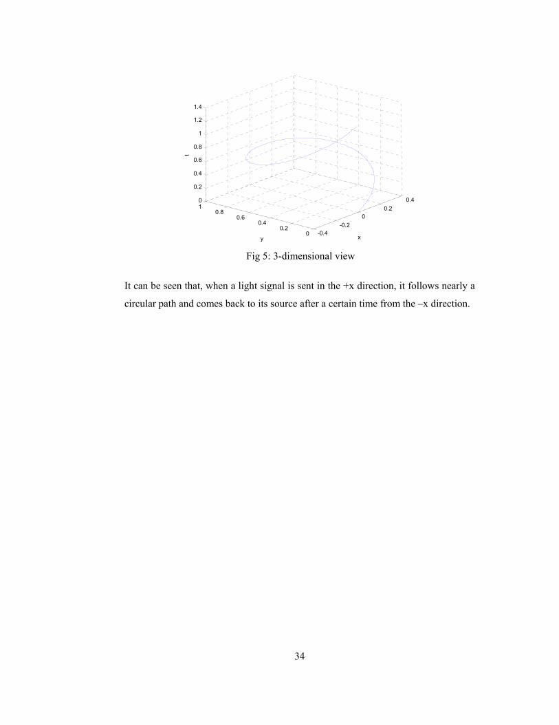
Fig 5: 3-dimensional view

It can be seen that, when a light signal is sent in the +x direction, it follows nearly a

circular path and comes back to its source after a certain time from the –x direction.