12 April 2010

GDP and Beyond Measuring Economic Progress and Sustainability By J. Steven Landefeld, Brent R. Moulton, Joel D. Platt, and Shaunda M. Villones

THE United States provides some of the most highly developed sets of gross domestic product

(GDP) accounts in the world. These accounts—which are collectively known as the national income and product accounts (NIPAs) or national accounts—have been regularly updated over the years and have well served researchers, the business community, and poli­cymakers alike. However, since their inception in the 1930s, the economy has continuously evolved, and is­sues have been raised about the scope and structure of the national accounts (Bureau of Foreign and Domes­tic Commerce and National Bureau of Economic Re­search 1934). Simon Kuznets (1941), one of the early architects of the accounts, recognized the limitations of focusing on market activities and excluding household production and a broad range of other nonmarket ac­tivities and assets that have productive value or yield satisfaction. Further, the need to better understand the sources of economic growth in the postwar era led to the development (much of it by academic researchers) of various supplemental series, such as the contribu­tions of investments in human capital and natural re­sources to economic growth.

More recently, concerns have been raised about the adequacy of the national accounts in capturing the dif­ferential impact of the current recession across house­holds, industries, and regions of the country. Concerns have also been raised about the failure of the national accounts to highlight and provide adequate warning about the imbalances that developed in housing and fi­nancial markets.

This article explores each of these issues and relates them to the need for expanded or supplementary mea­sures for the national accounts, highlighting what such estimates might reveal relative to the conventional sta­tistics presented by GDP and other aggregate statistics from the accounts. In particular, it explores how the accounts might be extended to provide new measures of (1) the distribution of growth in income across households, other sectors, and regions and (2) the sus­tainability of trends in saving, investment, asset prices, and other key variables important to understanding business cycles and the sources of economic growth.

Broad Social Accounts Kuznet’s concerns about the exclusion of a broader set of activities from the national accounts has been ech­oed over the ages, notably by Robert F. Kennedy in his eloquent critique of GDP as a measure of society’s progress.

Too much and too long, we seem to have sur­rendered community excellence and community values in the mere accumulation of material things. Our gross national product,1 if we should judge America by that, counts air pollution and cigarette advertising, and ambulances to clear our highways of carnage. It counts special locks for our doors…. Yet the gross national product does not allow for the health of our children, the qual­ity of their education, or the joy of their play … it measures everything, in short, except that which makes life worthwhile. And it tells us everything about America except why we are proud that we are Americans.

Robert F. Kennedy Address, University of Kansas, Lawrence, Kansas, March 18, 1968

This concern has remained an issue, and at his inau­gural address, President Barack Obama said

The success of our economy has always de­pended not just on the size of our gross domestic product, but on the reach of our prosperity; on the ability to extend opportunity to every willing heart—not out of charity, but because it is the surest route to our common good.

President Barack Obama, Inaugural Ad­dress, Washington, DC, January 20, 2009

The recent Report on the Measurement of Economic Performance and Social Progress addressed these issues.

The big question concerns whether GDP pro­vides a good measure of living standards. In

1. Gross national product is the market value of goods and services pro­duced by labor and property supplied by U.S. residents, regardless of where they are located. It was used as the primary measure of U.S. production prior to 1991, when it was replaced by GDP, which is that market value of goods and services produced within the United States.

13 April 2010 SURVEY OF CURRENT BUSINESS

many cases, GDP statistics seem to suggest that the economy is doing far better than most citi­zens’ own perceptions. Moreover, the focus on GDP creates conflicts: political leaders are told to maximize it, but citizens also demand that atten­tion be paid to enhancing security, reducing pol­lution, and so forth—all of which might lower GDP growth.

Stiglitz, Sen, Fitoussi (2009)

The Chair of the Commission that produced the re­port, Joseph Stiglitz, summarized the conclusions as follows:

The fact that GDP may be a poor measure of well-being, or even of market activity, has, of course, long been recognized. But changes in so­ciety and the economy may have heightened the problems, at the same time that advances in eco­nomics and statistical techniques may have pro­vided opportunities to improve our metrics.

Joseph Stiglitz (2009)

Work by Alan Krueger and others (2009) is the most recent comprehensive attempt to develop a broader measure of social welfare.2 Their “time-use accounts” develop a measure of happiness based on survey data on time use and happiness in different activities. Their accounts represent a significant step forward in the long quest to develop a broader measure of social wel­fare. They illustrate the progress that can be made by having such research conducted by a multidisciplinary team of independent researchers from academia. Their work also is an example of how various problems can be avoided by developing an entirely new measure with its own framework, concepts, and methods rather than by trying to expand GDP.

Past efforts to expand conventional GDP have foun­dered on the inevitable problems of subjectivity and uncertainty inherent in measuring health, happiness, and the environment.3 Critics feared that the inclusion of such uncertain and subjective values in GDP would seriously diminish the essential role of the national ac­

2. “National Time Accounting: The Currency of Life” includes analyses and critiques of the time-use accounts, including one comparing the time-use accounts to existing national accounts (Kruger and others 2009); see “National Time Accounting and National Economic Accounting” (Lande­feld and Villones 2009).

3. Work such as Nordhaus and Tobin (1973), the Genuine Progress Indi­cator (2007), the World Development Indicators (World Bank 2009), and the Index of Sustainable Economic Welfare are examples of the range of efforts that have been designed to spur further work on the regular produc­tion of broader measures of social welfare. While these efforts have been much discussed and debated, there has never been sufficient consensus on the difficult issues involved to produce a common set of concepts or meth­ods or a widely accepted regular set of estimates that were used for analyti­cal or policy purposes.

counts to financial markets, the Federal Reserve Board, the Treasury Department, and Congress in measuring and managing the market economy.

In recognition of these difficulties, several National Academy of Sciences studies on accounting for the en­vironment (Nordhaus and Kokkelenberg 1999) and nonmarket production (Abraham and Mackie 2005) and the System of National Accounts (1993) guidelines for compiling GDP have all concluded that an expan­sion of the GDP accounts should take place in supple­mental, or satellite, accounts that extend the scope of the accounts without reducing the usefulness of the core GDP accounts. They also conclude that such an expansion should focus on economic aspects of non-market and near-market activities—such as energy and the economy’s use of natural resources, the impact of investments in research and development (R&D), health care, or education—and not attempt to measure the welfare effect of such interactions.

Finally, such an expansion of work would require interdisciplinary research between economists and such subject area experts as epidemiologists, physi­cians, geologists, and engineers in other government agencies to measure the relationship among air pollu­tion and human health and medical expenditures or among petroleum extraction and changes in technol­ogy and reserves. It would also require the design, de­velopment, and collection of data from new surveys. In an environment of large competing demands on scarce resources, it is critical that such an expansion of the scope of the accounts not occur at the expense of funds needed to maintain, update, and improve the existing GDP accounts.

In recognition of the subjectivity, uncertainty, and resources involved in producing expanded welfare and nonmarket accounts, there is increasing interest in “new” estimates that could be produced with informa­tion currently used to produce the existing accounts. For example, the Stiglitz-Sen-Fitoussi commission (2009), which explored expanded welfare measures, has suggested a number of ways that “classical GDP is­sues” can be addressed within existing GDP accounts or through an extension and improvement of measures included in existing accounts.

What Can Be Done Within the Scope of the Existing Accounts?

Although the Bureau of Economic Analysis (BEA) has conducted research on a number of nonmarket satel­lite accounts and is currently at work on several mar­ket-related satellite accounts (for health care and R&D), relatively little attention has been paid to what can be done within the scope of the existing accounts

14 GDP and Beyond April 2010

to produce more relevant statistics.4 For example, for many households, the performance of GDP over the last economic expansion (2000–2007) does not seem to square with their personal experience. The growth in their take-home pay and bills seems to be very dif­ferent from the growth of officially reported “real” dis­posable income. Yet data are available from BEA’s national accounts and other data sources on the break­down of incomes, taxes, consumer outlays, and the prices households confront. That data can be used to construct cash and other alternate estimates of income that come closer to what most households are experi­encing. Further information from Internal Revenue Service (IRS) and other existing data could provide further insights into the distribution of household in­come.

Using statistics from BEA’s accounts and other exist­ing data, it is possible to construct new measures—and to highlight existing subcomponents of GDP—that would provide better indicators of, among other things, the differential impact of GDP growth across states, the sustainability of U.S. GDP growth, the ade­quacy of saving and investment, and emerging risks to the economy.

The next section of this paper discusses potential new measures of the distribution of growth across households, across regions of the country, and across different types of businesses. The last section of the pa­per discusses potential new measures of sustainability of trends in investment, saving, asset values, and fi­nance.

Income Growth Distribution Across Households, Regions, and Businesses

Household income The explanations for many of the differences between the individual experiences of households and the pic­ture of the economy captured in GDP, personal in­come, and other aggregate statistics can be found by drilling down below those aggregates in the national accounts and looking at the components and support­ing detail.

Compensation. Growth in real GDP, real income, and real compensation must be first put on a per capita

4. For more information on BEA’s satellite account work, see the follow­ing: “Integrated Economic and Environmental Satellite Accounts” (Lande­feld and Carson 1994b), “Accounting for Household Production” (Landefeld, Fraumeni, and Vojtech 2009), “Accounting for Nonmarket Household Production” (Landefeld and McCulla 2000), “U.S. Transporta­tion Satellite Accounts” (Fang, Han, Okubo, and Lawson 2000), “An Own­ership-Based Framework of the U.S. Current Account” (Lowe 2009), “BEA’s 2006 Research and Development Satellite Account” (Okubo, and others 2006), and “Toward a Health Care Satellite Account” (Aizcorbe, Retus, and Smith 2008).

or per worker basis to reflect something closer to the average worker’s experience. Part of the growth in pro­duction and income simply reflects the growth in the labor force and the larger wage bill that must be dis­tributed across a larger labor force.

Workers and households also confront different prices than producers, and at times, these prices change at quite different rates. For example, between the first quarter of 2007 and the third quarter 2008, rapid increases in energy costs resulted in consumer inflation, as measured by BEA’s personal consumption expenditures price index, which rose at an average an­nual rate of 3.8 percent. In contrast, overall GDP infla­tion, which is a measure of domestic production and excludes the prices of imported petroleum and other imported products, rose at an average annual rate of 2.4 percent. Due in large part to these different prices measures, growth in real GDP was 1.0 percentage point higher than the growth rate in real disposable in­come.

Taxes and noncash benefits also drive a wedge be­tween the aggregates and the typical worker’s experi­ence. BEA’s measure of disposable income addresses the tax issue by deducting taxes paid by households on their income. However, an alternate cash measure of disposable income would also deduct employer contri­butions to pension funds and contributions for health insurance and other benefits.5 These payments by em­ployers are a real cost of production (which must be re­corded in the double-entry NIPAs as income) and a real value to the employee. But when constructing a measure of cash income, noncash payments by em­ployers that are not available for current consumption should probably be deducted along with taxes. Because of the strong growth in employer “supplements,” pay­ments by employers for pensions, health insurance plans, and government social insurance, the difference between total compensation and take-home pay is of­ten large. Between 1967 and 2007, supplements, after adjustment for inflation, grew at an average annual rate of 3 percent, while real wages and salaries grew at an average annual rate of 1 percent.

Chart 1 illustrates the different perspectives on the economy that emerge by looking “below” the headline numbers. Between 2000 and 2007, the headline num­ber for real GDP grew at a 2.4 percent annual rate, and real compensation grew at a 2.1 percent annual rate.6

In comparison, over the same period, the below­the-headline numbers grew more slowly, with real

5. It would also exclude the interest and dividends earned by pension funds, which are included in personal income as part of personal interest and dividend income.

6. The period of 2000–2007 represents the peak-to-peak annual growth for the last business cycle.

15 April 2010 SURVEY OF CURRENT BUSINESS

compensation per worker growing at an average an­nual rate of 1.5 percent, real wages per worker (com­pensation less supplements) growing at an average annual rate of 1.2 percent, and real wages of produc­tion workers and nonsupervisory workers growing at an average annual rate of 0.3 percent (chart 2).

Personal income. Personal income is a broader measure than employment income and measures all income to households, including rent, interest income, dividends, and transfer payments, mainly from the government. Personal income also includes the income of nonprofit institutions. Transfer payments—such as social security, Medicare and Medicaid, unemploy­ment insurance, and other government programs—are important additions to the picture of household in­come. Because these payments tend to be countercycli-

Chart 1. Real Gross Domestic Product and Real Compensation

Percent

U.S. Bureau of Economic Analysis

Real GDP Real compensation

3.0

2.5

2.0

1.5

1.0

0.5

0

–0.5

–1.0

–1.5 Average growth, 2000–2007 2008

Chart 2. Spendable Income

cal, they have a large effect on growth in household income. As part of an effort to understand household spending and saving behavior as well as household welfare, it may be useful to decompose personal in­come in several different ways, including such mea­sures as cash income including transfers, market-based income excluding transfers, and discretionary income.

Disposable income, transfers, and the business cy­cle. BEA’s existing accounts provide two adjustments to household income that are useful in understanding household spending The first deducts taxes paid by households and provides a measure of disposable per­sonal income that is the after-tax income available for consumption or saving. The second deducts transfer payments in order to provide a better picture of the state of the private economy over the course of the business cycle and the incomes provided to households by the economy. The measure of personal income less current transfer receipts is shown as an addenda item in BEA personal income tables.

In 2008, transfer payments and lower taxes associ­ated with the economic stimulus acts helped boost real disposable personal income per capita. In 2008, per­sonal transfer payments increased $158 billion. Of that amount, approximately $30 billion were for rebates to persons under the Economic Stimulus Act of 2008. The same act reduced personal current taxes $66 bil­lion and more than accounted for the overall decrease in personal taxes of $59 billion in 2008. Such counter­cyclical transfers obscure changes in the components of income over the course of the business cycle, and they along with other transfer payments can cause dif­ferences across recipients of the transfers that are not reflected in the existing NIPA income aggregates.

As can be seen in chart 3, real GDP grew at an

Chart 3. Household Income: Alternative Measures

Percent

Source: BEA and BLS

Real compensation per worker Real wages per worker Real wages of production and nonsupervisory workers

2.0

1.5

1.0

0.5

0

0.5

–1.0 Average growth, 2000–2007 2008

Percent 3.0

2.0

1.0

0

–1.0

–2.0

–3.0

Real GDP Real DPI Real personal income per capita Real personal income less transfers per capita

Average growth, 2000–2007 2008

U.S. Bureau of Economic Analysis

16 GDP and Beyond April 2010

average annual rate of 2.4 percent over 2000–2007, and real disposable personal income grew at a 2.7 percent rate. Over the same period, real personal income per capita grew at a 1.5 percent rate, and real personal in­come less transfers per capita grew at a 1.2 percent rate. The countercyclical effect of government spending in 2008—including discouraged elderly workers decid­ing to “retire” and sign up for social security and Medi­care benefits and larger and longer claims for unemployment—is quite evident in the data for 2008; real personal income per capita contracted 1.3 percent; excluding transfers, it fell 2.4 percent.

Discretionary income. Another extension of BEA’s disposable income would be discretionary income, which would attempt to measure both the economic welfare of the average household and their ability to spend on big-ticket items over the course of business cycles. Discretionary income is calculated as the in­come left over after paying for basic household ex­penses. In other words, it measures the money that households can use for items, such as autos, vacations, entertainment, college educations, or put into savings.

Discretionary income, which is sometimes confused with disposable income, is used by investment firms to estimate funds available for saving or investment, by banks and credit card companies to estimate a custom­ers ability to take on mortgages and additional con­sumer debt, by marketers to identify households with discretionary income to spend on their products, and by individuals to plan personal budgets. The defini­tions of discretionary income vary, but used in these contexts, they are quite similar to those used in the poverty literature: income after taxes and after spend­ing on basic expenses, such as rent or mortgage, utili­ties, insurance, medical, transportation, child care, property maintenance, and food.7

Deducting the amount that consumers spend on such goods and services as food, shelter, and medical care can offer a rough notion of what households have left over to spend on more discretionary items. A mea­sure calculated in this manner would not aim to deter­mine how much spending on, say, food or housing is necessary. Indeed, during times of economic stress, a household may be able to cut back somewhat on their spending on food in the short run and in the longer run may be able to move to a less expensive house or apartment. Thus, basic expenses are not completely fixed, but they represent expenditures that are more difficult to adjust than expenditures on other, more discretionary goods and services.

7. Several investment banks including Deutsche Bank and Goldman Sachs have developed measures of discretionary income, which deduct taxes and basic or fixed expenses, and add net borrowings to obtain a mea­sure of cash discretionary income.

Exactly what should be deducted in deriving discre­tionary income will require further study. The defini­tion should reflect the purpose of the measure. If the purpose is to derive a measure of growth in household income, then the items to be deducted might be de­fined as a group of basic goods. Such goods would ac­count for a smaller share of spending by higher income households than for lower income households. How­ever, if the measure is intended as a measure for busi­ness cycle analysis, the definition might focus on goods and services whose share of spending tends to rise dur­ing downturns in economic activity as shrinking in­comes cause households to reduce their spending on discretionary spending more than their spending on the basics.

Chart 4 illustrates what a simple measure of real dis­cretionary income might look like. Over the last busi­ness cycle, the aggregate measure of growth, real GDP, grew at an average annual rate of 2.4 percent. Real dis­posable income per capita, however, grew at a 1.8 per­cent annual rate, and real discretionary income per capita grew at an average annual rate of 1.9 percent. (This larger growth rate reflects the lower inflation rate in discretionary income, which excludes food and en­ergy costs, than in disposable income; in nominal terms, discretionary income grew 4.9 percent, while disposable income grew 5.1 percent.) During the eco­nomic downturn of 2008, the differences are larger. Real GDP rose 0.4 percent, and real disposable per­sonal income per capita fell 0.4 percent. Real discre­tionary income per capita fell 1.3 percent.

In addition to the differences in growth rates, there are significant differences in levels between disposable and discretionary income. Between 2000 and 2007, average real disposable personal income per

Chart 4. Real GDP, Real Disposable Personal Income (DPI) and Real Discretionary Income Per Capita ,

Percent

Source: Experimental estimates based on BEA data

Real GDP Real DPI per capita Real discretionary income per capita

3.0

2.5

2.0

1.5

1.0

0.5

0

–0.5

–1.0

–1.5 Average growth, 2000–2007 2008

17 April 2010 SURVEY OF CURRENT BUSINESS

capita was $30,770, while average discretionary income was $16,333.

Refinements to the definition of discretionary in­come might well produce more useful results than those presented here. For example, the growth in dis­cretionary income and disposable income over the last business cycle in chart 4 may reflect the growth in aver­age income, including the gains in the share of income experienced by those in higher income brackets and may not reflect the experience of most households during that period. Household surveys during that pe­riod suggest that most households—as measured by real median income did not experience the growth in income or discretionary income shown in chart 4. And household surveys of consumer sentiment and of household’s assessment of the personal financial situa­tion showed significant declines between 2000 and 2007. (An example of what real median income and real discretionary income might look like based on tax data is shown in the next section.)

The small difference in growth also may reflect the need for a more detailed breakdown of spending on basic items. For example, how much of the increased spending on food and housing during this period was for steaks rather than hamburger, or for larger houses?

Alternatively, it may be necessary to rely on a defini­tion that uses spending by lower income households as a measure of basic spending such as that used in the poverty literature or another alternative used by the Conference Board (Franco 2007) and in an earlier Census Bureau study (1989). Those studies defined discretionary income as the incomes of households whose after-tax income was at least 30 percent higher than the average expenditures of households with sim­ilar characteristics (income, age, occupation, educa­tion, number of earners, and other demographic characteristics).

A refined measure of discretionary income might prove helpful in assessing the income that households have available to increase spending and saving over the course of the business cycle Such estimates would be especially helpful if paired with the type of integrated financial and household statistics described below to analyze changes in saving, debt, and net worth.

One such refinement of discretionary income would be to move from personal income, which includes sup­plements to wages as well as transfer payments, as a starting point to a cash-based measure, which excludes supplements but includes transfers. However, calculat­ing a cash measure for discretionary income would be difficult and would require disaggregation and sepa­rate estimates for different groups. For example, the discretionary income of workers and of retirees might look quite different. Working families’ cash incomes

would be reduced by taxes and contributions to pen­sions and health plans, while retired households’ cash incomes would be raised by transfer payments and pension payments. Further, working households may have higher spending on housing and other basics rela­tive to retired households. Such decomposition is pos­sible, but would require disaggregated income, spending, and transfer payment data from such sources as the Bureau of Labor Statistics (BLS) Survey of Consumer Expenditures, IRS data, Census Bureau Consumer Expenditure Survey data, and federal and state and local budget and program information.

Distribution of incomes. Per capita or other aver­age measures of income may not accurately reflect the economic position of most households. Adding infor­mation on median income or income growth by deciles to the national income accounts could signifi­cantly aid in tracking the distribution of gains from economic growth. The ability to decompose growth in the context of the national accounts is especially useful because the accounts provide a more comprehensive measure of income than that captured by most other measures. Income in the national accounts includes the noncash value of housing, financial and other ser­vices as well as noncash employer contributions for health insurance, pensions, and other benefits. It also adjusts for underreporting of income. As a result, the national accounts measures are broader than measures of hourly wages for production or nonsupervisory work, tax-based administrative data, or survey-based measures of median household income, which tend to underrepresent both noncash income and the incomes of low- and high- income groups.

National accounts measures of income have the ad­ditional advantage of being deflated by appropriate chain-weighted measures that address some of the weighting and other biases associated with fixed-weight indexes. The national accounts price indexes, such as the personal consumption expenditures price index, also are consistent in their coverage of items covered by the accounts.

As a result, national accounts-based estimates of av­erage incomes have led to discussions about the gains from economic growth. The main speculation has been on whether the higher average income growth shown in the national accounts reflects a more com­plete picture of household growth than the measures based on median income, which have grown more slowly.

Because one of the primary uses of the national ac­counts is measuring economic growth and the impact of growth on the nation’s income, there is increasing interest in understanding how the gains from growth are distributed. In recent years, evidence indicates that

18 GDP and Beyond April 2010

an increasing share of the gains from income growth have accrued to the upper income groups. Studies by Piketty and Saez (2007) using tax data, found that between 1993 and 2006, the average real income per family in the bottom 99 percent grew at about 1.1 per­cent per year. During the same period, however, aver­age real income growth per family in the top 1 percent was 5.7 percent. Data from household surveys con­ducted by the Census Bureau show a smaller difference in income growth between households at the top and the bottom of the distribution than IRS data but show a similar trend.

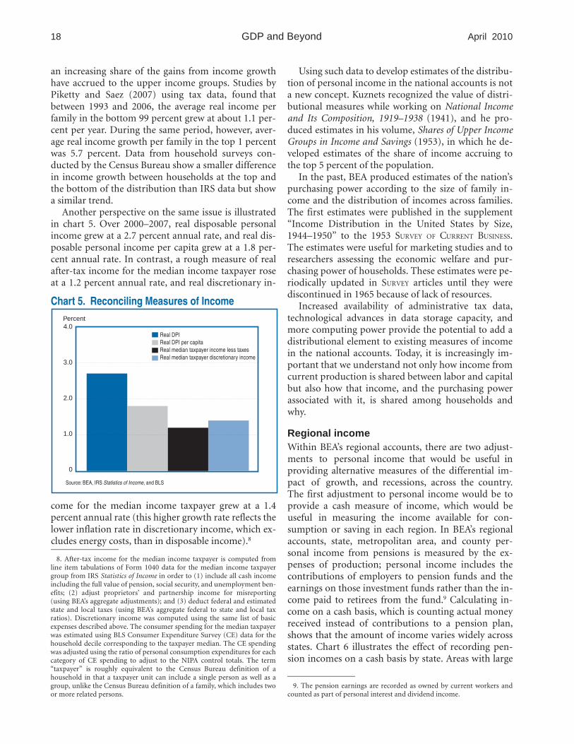
Another perspective on the same issue is illustrated in chart 5. Over 2000–2007, real disposable personal income grew at a 2.7 percent annual rate, and real dis­posable personal income per capita grew at a 1.8 per­cent annual rate. In contrast, a rough measure of real after-tax income for the median income taxpayer rose at a 1.2 percent annual rate, and real discretionary in-

Chart 5. Reconciling Measures of Income Percent 4.0

Real DPI Real DPI per capita Real median taxpayer income less taxes Real median taxpayer discretionary income

3.0

2.0

1.0

0

Source: BEA, IRS Statistics of Income, and BLS

come for the median income taxpayer grew at a 1.4 percent annual rate (this higher growth rate reflects the lower inflation rate in discretionary income, which ex­cludes energy costs, than in disposable income).8

8. After-tax income for the median income taxpayer is computed from line item tabulations of Form 1040 data for the median income taxpayer group from IRS Statistics of Income in order to (1) include all cash income including the full value of pension, social security, and unemployment ben­efits; (2) adjust proprietors’ and partnership income for misreporting (using BEA’s aggregate adjustments); and (3) deduct federal and estimated state and local taxes (using BEA’s aggregate federal to state and local tax ratios). Discretionary income was computed using the same list of basic expenses described above. The consumer spending for the median taxpayer was estimated using BLS Consumer Expenditure Survey (CE) data for the household decile corresponding to the taxpayer median. The CE spending was adjusted using the ratio of personal consumption expenditures for each category of CE spending to adjust to the NIPA control totals. The term “taxpayer” is roughly equivalent to the Census Bureau definition of a household in that a taxpayer unit can include a single person as well as a group, unlike the Census Bureau definition of a family, which includes two or more related persons.

Using such data to develop estimates of the distribu­tion of personal income in the national accounts is not a new concept. Kuznets recognized the value of distri­butional measures while working on National Income and Its Composition, 1919–1938 (1941), and he pro­duced estimates in his volume, Shares of Upper Income Groups in Income and Savings (1953), in which he de­veloped estimates of the share of income accruing to the top 5 percent of the population.

In the past, BEA produced estimates of the nation’s purchasing power according to the size of family in­come and the distribution of incomes across families. The first estimates were published in the supplement “Income Distribution in the United States by Size, 1944–1950” to the 1953 SURVEY OF CURRENT BUSINESS. The estimates were useful for marketing studies and to researchers assessing the economic welfare and pur­chasing power of households. These estimates were pe­riodically updated in SURVEY articles until they were discontinued in 1965 because of lack of resources.

Increased availability of administrative tax data, technological advances in data storage capacity, and more computing power provide the potential to add a distributional element to existing measures of income in the national accounts. Today, it is increasingly im­portant that we understand not only how income from current production is shared between labor and capital but also how that income, and the purchasing power associated with it, is shared among households and why.

Regional income Within BEA’s regional accounts, there are two adjust­ments to personal income that would be useful in providing alternative measures of the differential im­pact of growth, and recessions, across the country. The first adjustment to personal income would be to provide a cash measure of income, which would be useful in measuring the income available for con­sumption or saving in each region. In BEA’s regional accounts, state, metropolitan area, and county per­sonal income from pensions is measured by the ex­penses of production; personal income includes the contributions of employers to pension funds and the earnings on those investment funds rather than the in­come paid to retirees from the fund.9 Calculating in­come on a cash basis, which is counting actual money received instead of contributions to a pension plan, shows that the amount of income varies widely across states. Chart 6 illustrates the effect of recording pen­sion incomes on a cash basis by state. Areas with large

9. The pension earnings are recorded as owned by current workers and counted as part of personal interest and dividend income.

19 April 2010 SURVEY OF CURRENT BUSINESS

pension contributions—such as the District of Colum­bia, Maryland, and Virginia, each with a large number of federal workers—have lower cash personal income than personal income. Other states, such as Florida, with large retirement populations and lots of income receipts from retirement funds (and lower wage and salary incomes) tend to have higher cash incomes.

Another adjustment would be to develop estimates of the “real” incomes received by households across re­gions by adjusting for differences in regional prices. Chart 7 uses experimental work by BEA and BLS on

Chart 6. Difference If Retirement Income is Included in State of Current Residence

regional prices to develop illustrative real estimates by state. As can be seen, there are significant differences in “real” per capita personal income due to differences in prices across states. More rural, lower cost-of-living states—such as West Virginia, North Dakota, and Mis­souri—would see their income per capita raised rela­tive to urban and higher cost-of-living areas, such as New York, the District of Columbia, and Hawaii.

The experimental estimates of regional prices and real income presented here are based on work by Aten and D’Souza (2008). They used price data that are

Chart 7. Difference After Adjusting for Regional Prices

Source: Experimental estimates based on BEA regional data

–6 –4 –2 0 2 4 6 8 10 12 14

Billions of dollars

Maryland Virginia

California Minnesota Wisconsin Colorado

D.C. Connecticut

Massachusetts Georgia

North Carolina Hawaii

Delaware Alaska

Oregon Maine Illinois

Indiana Mississippi

Ohio Oklahoma

New Hampshire Idaho

Rhode Island North Dakota

Iowa Kansas

Louisiana New Jersey

South Dakota Missouri

New Mexico Montana

Nebraska Wyoming Vermont

Washington West Virginia

Alabama Arkansas Kentucky

Nevada Tennessee

Utah South Carolina

Arizona Texas

New York Pennsylvania

Michigan Florida

Source: Aten and D’Souza 2008

–8,000 –6,000 –4,000 –2,000 0 2,000 4,000 6,000 8,000

West Virginia North Dakota

Missouri Arkansas Kentucky Alabama

Iowa Kansas

Oklahoma Indiana

South Dakota Louisiana

Mississippi South Carolina

Idaho Tennessee

Montana New Mexico

Wyoming Nebraska

North Carolina Ohio Utah

Georgia Minnesota Wisconsin

Texas Michigan

Maine Pennsylvania

Arizona Oregon

Colorado Delaware

Illinois Vermont

Florida Nevada Virginia

Washington Maryland

Alaska Rhode Island

New Hampshire Massachusetts

Connecticut New Jersey

California Hawaii

D.C. New York

Billions of dollars

20 GDP and Beyond April 2010

available across all states, mainly Census Bureau hous­ing price data, and the relationship between those prices and the prices of all other goods and services in the BLS urban areas to estimate average prices for all goods and services for the 50 states and the District of Columbia. (Because metropolitan areas account for such a large share of overall prices and each state’s eco­nomic activity and given the share of housing in over­all prices, the extrapolation seems to produce reasonable results.) However, further work needs to be done toward developing methodologies that ensure that growth in the extrapolated annual state price in­dexes are consistent with the growth in BLS area and BEA national price indexes. Also, benchmark estimates may be needed to more solidly anchor estimates for states less well covered by BLS urban area statistics. Fi­nally, the initial work by Aten and D’Souza needs to be modified to be consistent with the coverage and defini­tions of personal income.

Business income In addition to wages and salaries, income from sole proprietors, partnerships and other small businesses is an important component of household income and an indicator of how well the average household is doing. Despite the importance of this type of income, there is no integrated picture of small business activity in the national accounts, and existing aggregates of business activity and income often obscure the differential change in the condition of small businesses versus large businesses and the change across industries and regions. Business income in the national accounts is split between corporate and noncorporate income and within noncorporate income between farm and non­farm income. This limited detail provides limited in­formation to aid policymakers in formulating the many programs targeting assistance to small business.

A significant portion of business income in the NIPAs is currently benchmarked to IRS tax return data. In addition to their current importance in mea­suring aggregate business, tax data can also be a rich source of information for measuring the contributions made to GDP and household income by small busi­nesses. Alternative measures of business income could be considered that focus on business characteristics rather than on legal form of organization (that is, cor­porate income versus proprietors’ income), that better isolate the business income passed through directly to households, or that provide information that identifies contributions to growth in business income by busi­nesses of different sizes, where size may be identified, for example, by size of assets or total receipts.

It could be argued that the current distinction be­

tween corporate and noncorporate business income obscures the economic contributions of certain small businesses organized as Subchapter S-corporations (S-corps). Unlike generally larger Subchapter C-corpo­rations (C-corps), S-corps do not pay a corporate level income tax, and for tax purposes, business income is passed directly through to business owners. In the na­tional accounts, business income and profits of both C-corps and S-corps are aggregated in the measure of corporate profits. This presentation masks the differ­ential growth rates and changing contributions to cor­porate profits between C-corps and S-corps in recent years. For example, according to IRS data, between 1994 and 2006, S-corps as a share of the number of to­tal corporate businesses increased from 46.7 percent to 68.4 percent (chart 8). As a share of total busi­ness receipts for corporations, the share attributable to S-corps increased from 18.3 percent in 1994 to 26.2 percent in 2006.

Chart 8. S-Corp Share of Total Number of Businesses and Total Business Receipts

Percent 80

70

60

50

40

30

20

10

0

Share of total number of corporations Share of total corporate business receipts

1994 95 96 97 98 99 2000 01 02 03 04 05 06

Source: IRS Statistics of Income

BEA is examining the feasibility of developing sup­plemental measures of small business based on IRS tax data, BLS and Census Bureau work on small business employment and growth, and other research on small business and its role in the economy.

Assessing the Sustainability of Trends in the Economy

Public and private decisionmakers tasked with assess­ing the sustainability of trends in the economy would also benefit from highlighting various data that are al­ready included in the national accounts or that could be derived from the existing national accounts and their underlying source data.

21 April 2010 SURVEY OF CURRENT BUSINESS

Net domestic product and net investment Since the U.S. national accounts were developed in the 1930s by Simon Kuznets and his colleagues, there has been a recognition of the need to calculate a measure of income and production that nets out the capital and natural resources used up in production. Similarly, business accounting deducts the cost of depreciation and depletion in calculating profits.

In the national accounts, the “G” in GDP stands for gross to indicate that depreciation has not been sub­tracted out. Net domestic product is equal to GDP less depreciation or what BEA calls the consumption of fixed capital. Net domestic product is a rough measure of sustainable income, that is, the amount of con­sumption that is sustainable after putting aside the amount of resources necessary to replace the produc­tive capital stock used up in production. Alternatively, it can be described as the amount that can be con­sumed without reducing the consumption of future generations.

BEA has produced estimates of net domestic prod­uct and net domestic income for decades, but they have received little attention. Yet over time, real net do­mestic product and real net domestic income can pro­duce significantly different estimates than the commonly referenced GDP and gross domestic in­come estimates. For example, between 2000 and 2007, GDP grew at a 2.4 percent annual rate, and net domes­tic product (NDP) grew at a 2.2 percent rate (chart 9). During the downturn in 2008, GDP increased 0.4 per­cent, while net domestic product was unchanged.

BEA also produces estimates of net domestic invest­ment, which deducts depreciation from gross domestic fixed investment for a measure of net additions to wealth. Like net domestic income, net fixed investment looks quite different from gross investment (chart 10).

For example, between 2000 and 2007, on average, nearly 62 percent of gross business investment simply replaced capital used up in the production process; that is, only $927 billion of the nearly $2.4 trillion in gross business fixed investment represented a net addi­tion to the future productive potential of the domestic capital stock. Over time, the two measures also pro­duce quite different results. For example, over the last business cycle, gross investment grew at 1.5 percent, while net domestic investment contracted 1.9 percent.

Asset values, saving, and consumption The notion of sustainability is also relevant to the housing and financial bubbles that the nation experi­enced over the last decade and their impact on saving, consumption, and overall economic performance.

Although the existing GDP and related accounts did a good job in measuring the evolving path of the real

economy, supplementary data derived from integrated financial accounts might have helped policymakers, analysts, and investors by highlighting how out of line housing and equity prices were and how big an adjust­ment was required. New statistics that better highlight emerging trends in markets could focus attention on asset price anomalies and affect policy in the way that GDP, inflation, or the unemployment rate affect fiscal and monetary policy. While some attribute the current downturn to the effect of monetary policy on asset in­flation and of regulatory policies that failed to confront excessive risk taking, good statistics can play a key role in forming public policy by highlighting the magni­tude of emerging problems and by aiding in the build­ing of public consensus about policy action.

Chart 9. Real Gross Domestic Product and Real Net Domestic Product

Percent

U.S. Bureau of Economic Analysis

Real GDP Real NDP

3.0

2.5

2.0

1.5

1.0

0.5

0 Average growth, 2000–2007 2008

0.0

Chart 10. Real Gross Domestic Investment and Real Net Domestic Investment

Percent

U.S. Bureau of Economic Analysis

Real gross domestic investment Real net domestic investment

5

0

–5.0

–10.0

–15.0

–20.0

–25.5 Average growth, 2000–2007 2008

22 GDP and Beyond April 2010

Chart 11 shows the rise in the value of the U.S. housing stock relative to personal income and GDP. Between 2000 and 2007, the value of the U.S. housing stock rose from 1.1 times personal income to 1.4 times personal income, as housing prices rose an average 9.2 percent annually, while personal income rose an aver­age 4.8 percent annually. While part of this increase in housing prices was driven by a drop in mortgage rates, ultimately housing prices are dependent on personal income or expected future capital gains on housing in­vestment. At some point, the price increase was signal­ing what later turned out to be an unsustainable bubble. The regular publication of ratio data such as the ratio of the value of housing to personal income shown in chart 11 along with data on leveraging in housing markets shown in chart 13 might have been helpful in recognizing the size and extent of that bub­ble earlier. Additional ratio data of household net worth to personal income, which was rising over this

Chart 11. Housing and Personal Income Ratio 2.0

1.8

1.6

1.4

1.2

1.0

0.8

0.6

0.4

Source: BEA and Federal Reserve Board flow of funds

Chart 13. Household Asset Values and Saving Index numbers, 1980:I=1.00

1.60

1.40

1.20

1.00

0.80

0.60

0.40

0.20

0.00

–0.20

Source: BEA and Federal Reserve Board flow of funds

period, help to understand households’ willingness to take on incremental debt (chart 13).

Chart 12 shows the rise in U.S. equity prices relative to GDP (log scale) since the mid-1990s. In the latter half of the 1990s, higher growth in GDP and produc­tivity, new technologies, and higher expectations for trend growth in GDP helped to raise growth in stock prices substantially relative to GDP; the run-ups that ended in 2000 and 2008 were followed by 41 and 48 percent declines in stock prices, respectively.

Over the long run, equity prices rise at roughly the same rate as GDP and corporate profits. Between 1977 and 2009, stock prices and GDP both rose at an aver­age annual rate of roughly 7 percent. This makes sense because over time, growth in stock prices must come from growth in the economy or a higher rate of return to capital investments. However, there have been peri­ods when growth in stock prices consistently outpaced

Chart 12. Growth of Equity Prices Relative to Growth of Gross Domestic Product

1977 79 81 83 85 87 89 91 93 95 97 99 2001 03 05 07 09

Log scale

100.00

10.00

1.00

0.10

Source: BEA and Standard & Poor’s

Nominal GDP

S&P 500 Index

Value of household real estate assets/Personal income

Household total liabilities/Personal income

0.2

0.0 1970 72 74 76 78 80 82 84 86 88 90 92 94 96 98 00 02 04 06 08

Personal saving rate

Net worth as a percent of DPI

1980 81 82 83 84 85 86 87 88 89 90 91 92 93 94 95 96 97 98 99 2000 01 02 03 04 05 06 07

23 April 2010 SURVEY OF CURRENT BUSINESS

growth in GDP, particularly the period in the 1950s and 1960s, which was followed by a market correction and then a prolonged period when growth in stock prices consistently lagged GDP. The historical record is a useful reminder that identifying divergences from trend is easier than predicting when trends will end. Nonetheless, regularly presenting data on the relation­ship between asset prices and underlying real variables can be important to investors and policy officials mon­itoring monetary, fiscal, and regulatory policies that af­fect asset prices.

Chart 13 shows the share of the increase in house­hold net worth (saving) that came from saving out of current income as compared with capital gains on homes or investments. Between 2000 and 2007, house­holds saw their net worth rise from $42.0 trillion to $62.6 trillion.10 In response, households saw little need to save out of current income; the personal saving rate dropped from 2.3 percent to 0.6 percent. There seemed to be little need for households to be concerned about the future because “saving” through appreciation in their portfolio was more than offsetting the drop in their saving out of current income, and the ratio of net worth to disposable income was actually increasing. These unsustainable trends—based on the unsustain­able rise in housing and equity prices—not only had significant implications for the adequacy of household retirement assets but also significant implications for the U.S. and world economy; U.S. saving out of current income has risen significantly since the recession be­gan, and the share of U.S. GDP accounted for by con­sumer spending has fallen to below 70 percent.

These figures, which are based on available data, il­lustrate how far out of line prices were in the housing and stock markets and the extent to which the house­hold saving rate out of current income was unsustain­able. If BEA were to expand its dissemination of charts and analytical ratios such as these, this information could be useful to decisionmakers who need to identify and anticipate future imbalances.

There was also a gap in macroeconomic data to warn of growing imbalances in credit markets. As Palumbo and Parker (2009) have shown, available data only show a slightly higher average leverage ratio in the financial sector—1.03 in the late 1990s, compared with an average ratio of 0.97 over the previous two de­cades—indicating that the U.S. data are too aggregated to isolate the dramatic increase in leveraging that was taking place in mortgage banks, other financial institu­tions, and special purpose entities (chart 14).

10. Federal Reserve Board flow of funds data; available at www.federal reserve.gov/econresdata/default.htm.

Because the data were too aggregated, detailed data on maturity of financial instruments to identify mis­alignment of assets and liabilities—such as detailed data by type of instrument, such as how much of U.S. international bond sales were of collateralized sub-prime loans—were also missed.

A more complete list of data that would be required to address the gaps in the financial data include (1) more complete data on those institutions that played a large role in the crisis—hedge funds, private equity funds, structured investment vehicles, (2) more de­tailed data by type of instrument, by maturity, on valu­ation by type of instrument, by ultimate owner rather than counterparty, and on special purpose entities, and (3) more data on leverage by institution and instru­ment.

All of these data could be collectible through the ex­isting reporting systems of the Treasury Department and the Federal Reserve Board and should correspond with information required under any new regulatory reporting systems that emerge from the proposals cur­rently before the Congress.

Through new data and the publication of charts and analytic ratios, BEA could provide additional tools for macroeconomic analysts and policymakers. In the past, BEA produced a monthly journal, Business Con­ditions Digest, and a special cyclical indicators section of the SURVEY that presented analytic information on evolving economic conditions in charts and ratios. The Business Conditions Digest and the cyclical indicators section were eliminated as a result of budget con­straints. While the return to the publication of the leading indicators component of those charts and ra­tios is not consistent with BEA’s mission and would be

Chart 14. Financial Business Sector Leverage

Source: BEA/Federal Reserve Board integrated U.S. macroeconomic accounts

1.15

1.10

1.05

1.00

0.95

0.90

0.85 1970 72 74 76 78 80 82 84 86 88 90 92 94 96 98 00 02 04 06

Ratio

24 GDP and Beyond April 2010

duplicative of private sector efforts, the publication of selected ratios and data on sustainability, such as those discussed above, might be an efficient means of pro­viding economists with tools they could use to address the integration of risk, finance, and the real economy currently being called for by voices within and outside the economic profession.11

Next Steps This paper has presented possible alternative measures of economic activity that could expand the usefulness of the existing national accounts in understanding the distribution of the growth in incomes and the sustain-ability of trends in the economy and their implications for future growth. Few of the proposals here are com­pletely new, and some of the suggestions are nearly as

11. See Coy (2009), “What Went Wrong With Economics? (2009), and Stiglitz (2009).

old as the initial set of national income accounts devel­oped by Kuznets and others. However, the magnitude of the current downturn and the differences between aggregate growth and growth across households, sec­tors, and regions of the country suggest the need for a review of the use of the national accounts, which were first developed during the great depression.

The development of such new data will follow the steps that BEA has always taken in the development of new estimates. First, the methods, source data, and ex­perimental estimates will be subjected to an internal and external review to ensure that they meet BEA’s standards for accuracy, reliability, timeliness, and rele­vance. Second, prototype estimates will be published for public comment by users of the national accounts. Finally, after this period of review and adjustment is completed, BEA will begin regular publication of these new and more detailed data as part of its regular monthly, quarterly, and annual estimates.

References Abraham, Katherine G., and Christopher Mackie, eds. 2005. Beyond the Market: Designing Nonmarket Ac­counts for the United States. Washington DC: National Academy Press.

Aizcorbe, Ana M., Bonnie A. Retus, and Shelly Smith. 2008. “Toward a Health Care Satellite Account.” SURVEY OF CURRENT BUSINESS 88 (May): 24–30.

Aten, Bettina H. 2006. “Interarea Price Levels: An Experimental Methodology.” Monthly Labor Review 126 (September): 47–61.

Aten, Bettina H., and Roger J. D’Souza. 2008. “Re­gional Price Parities: Comparing Price Level Differ­ences Across Geographic Areas.” SURVEY OF CURRENT

BUSINESS 88 (November): 64–69. Blank, Rebecca M., and Mark H. Greenburg. 2008.

Improving the Measurement of Poverty. Discussion pa­per 2008–17. Washington, DC: The Hamilton Project, The Brookings Institution (December); www.brook ings.edu/papers/2008.

Bureau of Foreign and Domestic Commerce and National Bureau of Economic Research. 1934. National Income, 1929–32. Report to Congress. Washington, DC: U.S. Government Printing Office.

Census Bureau. 1989. A Marketer’s Guide to Discre­tionary Income. Washington, DC: U.S. Government Printing Office.

Citro, Constance F., and Robert T. Michael, eds. 1995. Measuring Poverty: A New Approach. Washing­ton, DC: National Academies Press.

Coy, Peter. 2009. “What Good Are Economists Anyway?” BusinessWeek (April 27); www.business week.com.

Fang, Bingsong, Xiaoli Han, Sumiye Okubo, and Ann M. Lawson. 2000. “U.S. Transportation Satellite Accounts for 1996.” SURVEY OF CURRENT BUSINESS 80 (May): 14–23.

Franco, Lynn. 2007. The Marketer’s Guide to Discre­tionary Income. New York: The Conference Board Re­search Center.

Jorgenson, Dale W., J. Steven Landefeld, and Will­iam D. Nordhaus, eds. 2006. A New Architecture for the U.S. National Accounts. Chicago: University of Chicago Press.

Krueger, Alan B., Daniel Kahneman, David Sch­kade, Norbert Schwarz, and Arthur A. Stone. 2009. “National Time Accounting: The Currency of Life.” In Measuring the Subjective Well-Being of Nations: Na­tional Accounts of Time Use and Well-Being, ed. Alan B. Krueger, 113–123. Chicago: University of Chicago Press for NBER.

Kuznets, Simon. 1941. National Income and Its Composition, 1919–1938. New York: NBER.

25 April 2010 SURVEY OF CURRENT BUSINESS

Kuznets, Simon, assisted by Elizabeth Jenks. 1953. Shares of Upper Income Groups in Income and Savings. New York: NBER.

Landefeld, J. Steven, and Carol S. Carson. 1994a. “Accounting for Mineral Resources: Issues and BEA’s Initial Estimates.” SURVEY OF CURRENT BUSINESS 74 (April): 50–72.

Landefeld, J. Steven, and Carol S. Carson. 1994b. “Integrated Economic and Environmental Satellite Accounts,” SURVEY OF CURRENT BUSINESS 74 (April): 33–49.

Landefeld, J. Steven, and Stephanie H. McCulla. 2000. “Accounting for Nonmarket Household Produc­tion Within a National Accounts Framework.” Review of Income and Wealth 46, no. 3 (September): 289–307.

Landefeld, J. Steven, and Shaunda Villones. 2009. “National Time Accounting and National Economic Accounting.” In Measuring the Subjective Well-Being of Nations: National Accounts of Time Use and Well-Being, ed. Alan B. Krueger, 113–123. Chicago: University of Chicago Press for NBER.

Landefeld, J. Steven, Barbara M. Fraumeni, and Cindy M. Vojetch. 2009. “Accounting for Household Production: A Prototype Satellite Account Using the American Time Use Survey.” Review of Income and Wealth 52, no. 2 (June): 205–255.

Lowe, Jeffrey H. 2009. “An Ownership-Based Framework of the U.S. Current Account, 1998–2007.” SURVEY OF CURRENT BUSINESS 89 (January): 62–64.

Nordhaus, William D., and Edward C. Kokkelen­berg, eds. 1999. Nature’s Numbers: Expanding the Na­tional Economic Accounts to Include the Environment. Washington, DC: National Academy Press.

Nordhaus, William D., and James Tobin. 1973. “Is Growth Obsolete?” In The Measurement of Economic and Social Performance, ed. Milton Moss, 509–534. New York: Columbia University Press.

Office of Business Economics, U.S. Department of

Commerce. 1953. “Income Distribution in the United States by Size, 1944–1950.” SURVEY OF CURRENT BUSINESS

33 (supplement). Okubo, Sumiye, Carol A. Robbins, Carol E. Moylan,

Brian K. Sliker, Laura I. Shultz, and Lisa S. Mataloni. 2006. “BEA’s 2006 Research and Development Satellite Account.” SURVEY OF CURRENT BUSINESS 86 (December): 14–27.

Palumbo, Michael G., and Jonathan A. Parker. 2009. “The Integrated Financial and Real System of National Accounts for the United States: Does It Presage the Fi­nancial Crisis?” American Economic Review 99 (Febru­ary): 80–86.

Piketty, Thomas, and Emmanuel Saez. 2007. “In­come and Wage Inequality in the United States, 1913–2002.” In Top Incomes Over the Twentieth Cen­tury: A Contrast Between European and English-Speak­ing Countries, eds. Anthony B. Atkinson and Thomas Piketty, 141–226. Oxford: Oxford University Press. Ta­bles and figures updated to 2007 at elsa.berkeley.edu/ ~saez.

Refining Progress. 2007. Genuine Progress Indica­tor; www.rprogress.org.

Stiglitz, Joseph E. 2009. “GDP Fetishism.” The Econ­omists’ Voice (September); www.bepress.com.

Stiglitz, Joseph E., Amartya Sen, and Jean-Paul Fi­toussi. 2009. Report by the Commission on the Measure­ment of Economic Performance and Social Progress; www.stiglitz-sen-fitoussi.fr/en/index.htm.

United Nations, Commission of the European Communities, International Monetary Fund, Organi­sation for Economic Co-operation and Development, and World Bank. 1993. System of National Accounts, 1993. New York: United Nations.

“What Went Wrong With Economics.” 2009. The Economist. (July 16).

The World Bank. 2009. World Development Indica­tors, 2009. Washington, DC: The World Bank.