GEM4 Summer School OpenCourseWare http://gem4.educommons.net/ http://www.gem4.org/

Lecture: “Microrheology of a Complex Fluid” by Dr. Peter So. Given August 10, 2006 during the GEM4 session at MIT in Cambridge, MA.

Please use the following citation format:

So, Peter. “Microrheology of a Complex Fluid.” Lecture, GEM4 session at MIT, Cambridge, MA, August 10, 2006. http://gem4.educommons.net/ (accessed MM DD, YYYY). License: Creative Commons Attribution-Noncommercial-Share Alike.

Note: Please use the actual date you accessed this material in your citation.

Microrheology of Complex Fluid

� Rheology: Science of the deformation & flow of matter

� Microrheology

Complex shear modulus G*(ω)

σ = G* ε

Storage modulus G’ Energy storage Elasticity ~ Solid

- Microscopic scale samples

- Micrometer lengths

Image removed due to copyright restrictions.

- G* (ω) = G’ (ω) + j G’’ (ω) Loss modulus G’’ Image removed due to- Solid vs. fluid Energy dissipationcopyright restrictions.

- Resistance to deformation Viscosity ~ Fluid

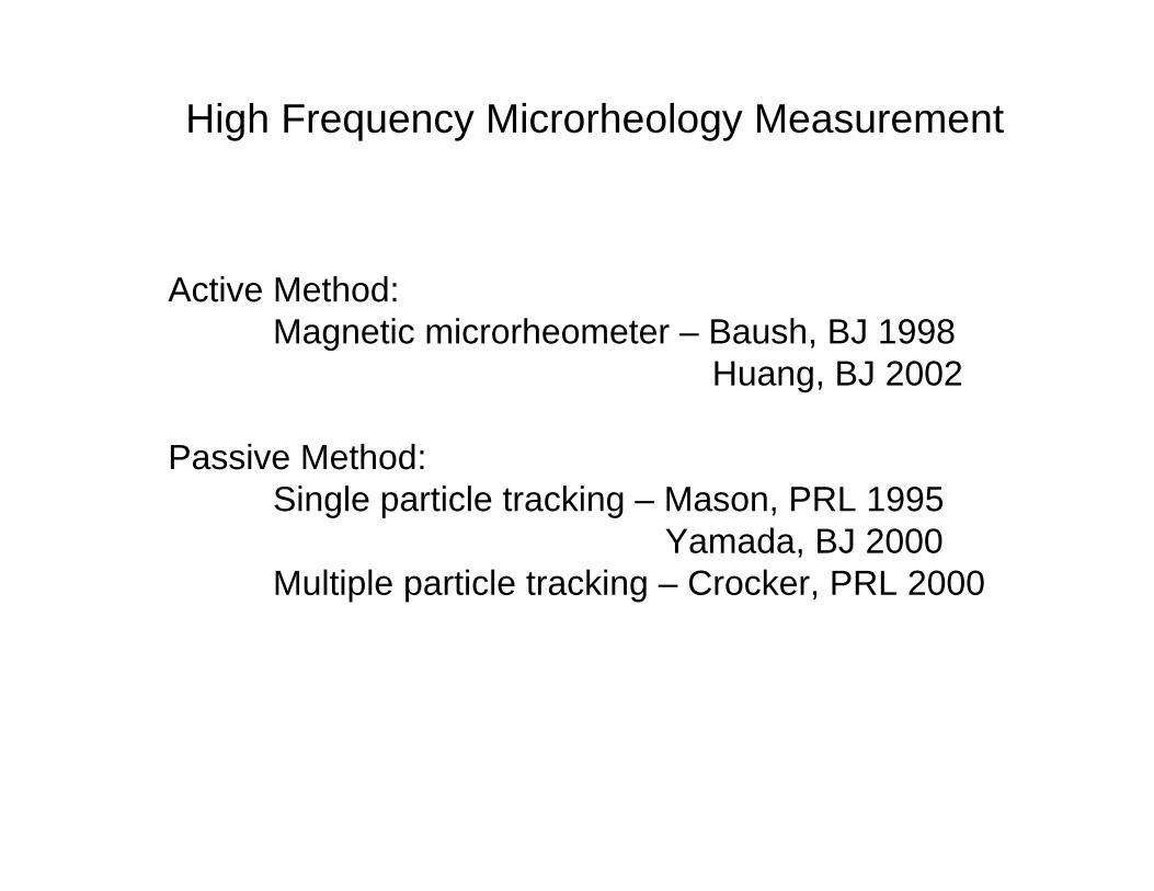
High Frequency Microrheology Measurement

Active Method: Magnetic microrheometer – Baush, BJ 1998

Huang, BJ 2002

Passive Method: Single particle tracking – Mason, PRL 1995

Yamada, BJ 2000 Multiple particle tracking – Crocker, PRL 2000

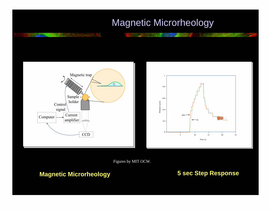
Magnetic Microrheology

Magnetic Microrheology 5 sec Step Response

1

0.8

0.6

0.4

0.2

Dis

tanc

e (µ

m)

5 10 15 20 25

Time (s)

0

Figures by MIT OCW.

Sample holder

Magnetic trap

Control signal

Computer Current amplifier

CCD

data

fit

Basic Physics of Magnetic Microrheometer

Ferromagnetic particle

F m H) = ∇ ⋅ 1 2 0µ (

Particles cluster together! Doesn’t work!

Paramagnetic particle – no permanent magnetic moment

F H H = ∇ ⋅µ χ0 V )( χ is suceptibility

V is volume

Note: (1) force depends on volume of particle (5 micron bead provide 125x more force)

(2) force depends on magnetic field GRADIENT

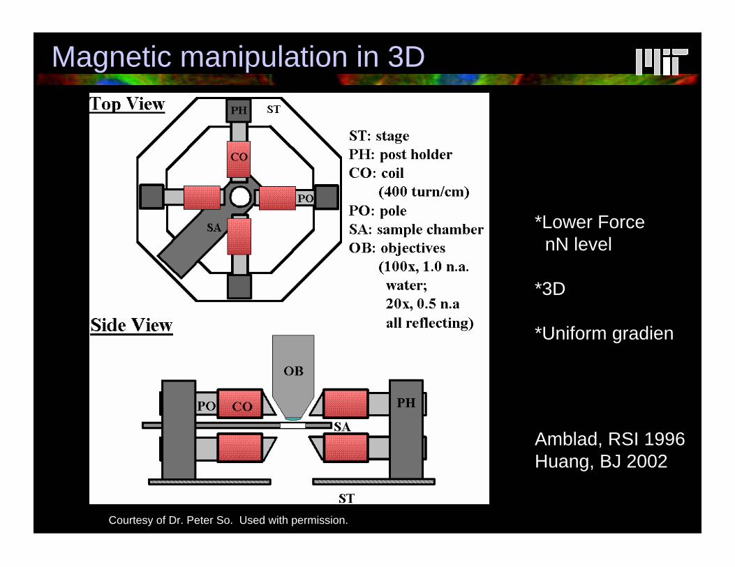
Magnetic manipulation in 3D

Amblad, RSI 1996 Huang, BJ 2002

*Lower Force nN level

*3D

*Uniform gradien

Courtesy of Dr. Peter So. Used with permission.

Magnetic manipulation in 1D

*High force >10 nN

*Field non-uniform Needs careful alignment of tip to within microns

*1D

The bandwidth of ALL magnetic microrheometer is limited by the inductance of the eletromagnet to about kiloHertz

Figure by MIT OCW. After Bausch et al., 1998.

r

Magnet Sample chamber

Cover glass

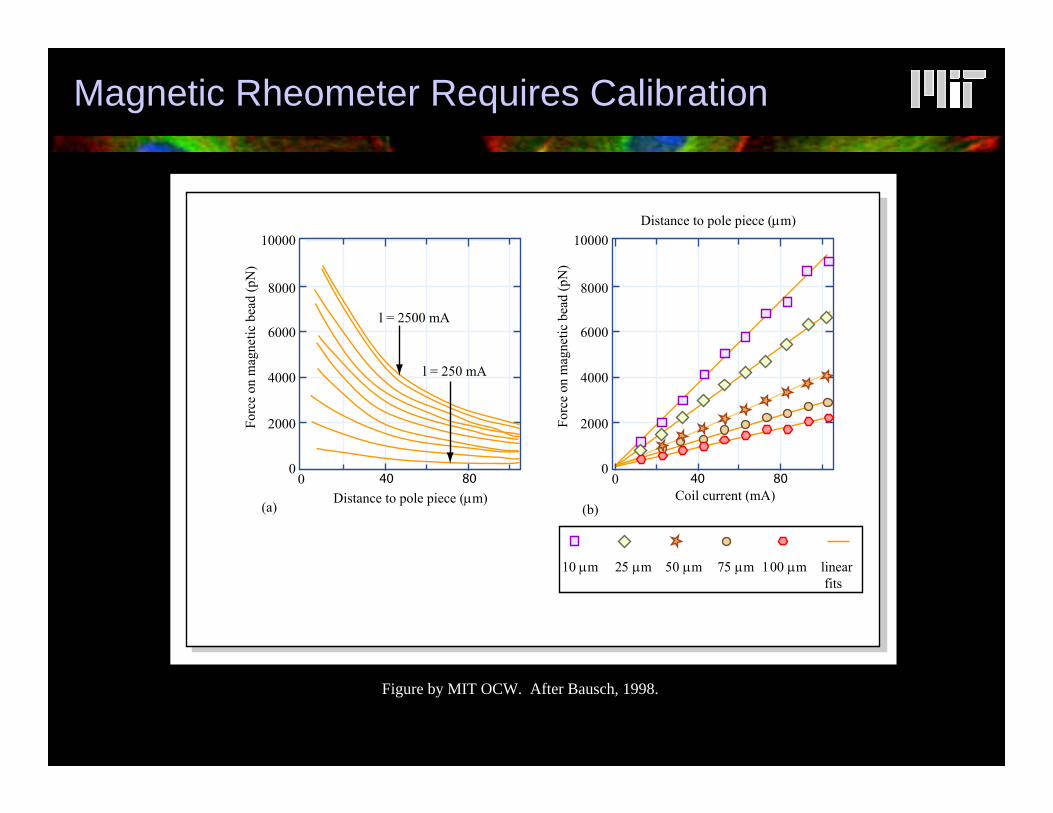
Magnetic Rheometer Requires Calibration

Distance to pole piece (µm)

0

2000

4000

6000

8000

10000

l = 2500 mA

l = 250 mA

Forc

e on

mag

netic

bea

d (p

N)

0

2000

4000

6000

8000

10000

Forc

e on

mag

netic

bea

d (p

N)

0 40 80 0 40 80

Distance to pole piece (µm) Coil current (mA)(a) (b)

10 µm 25 µm 50 µm 75 µm 100 µm linear fits

Figure by MIT OCW. After Bausch, 1998.

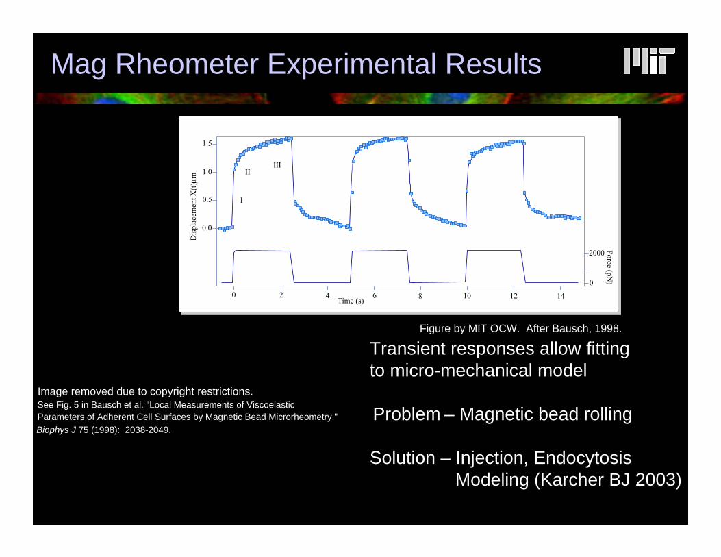
Mag Rheometer Experimental Results

Transient responses allow fitting to micro-mechanical model

Image removed due to copyright restrictions. See Fig. 5 in Bausch et al. "Local Measurements of Viscoelastic Parameters of Adherent Cell Surfaces by Magnetic Bead Microrheometry."metry." Problem – Magnetic bead rolling Biophys J 75 (1998): 2038-2049.

Solution – Injection, Endocytosis Modeling (Karcher BJ 2003)

I

II III

1.5

1.0

0.5

0.0

Dis

plac

emen

t X(t)

µm

0 2 4 6 8 10 12 14

2000

0

Force (pN)

Time (s)

Figure by MIT OCW. After Bausch, 1998.

Model Strain Field Distribution

Image removed due to copyright reasons. See Fig. 9 in Bausch et al. "Local Measurements of Viscoelastic Parameters of Adherent Cell Surfaces by Magnetic Bead Microrheometry." Biophys J 75 (1998): 2038-2049.

New Text

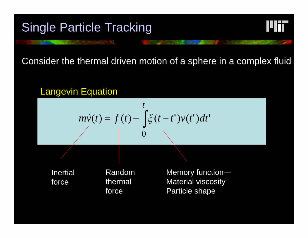
Single Particle Tracking

Consider the thermal driven motion of a sphere in a complex fluid

Langevin Equation

∫ −+= t

dttvtttftvm0

')'()'()()( ξ&

Inertial Random Memory function— force thermal Material viscosity

force Particle shape

Langevin Equation in Frequency Domain

mss mvsf sv +

+ =

)( ~ )0()( ~

)(~ξ

Laplace transform of Langevin Equation

6/)(~)(~)0(

)(~)( ~ )(~6)(

)0()0(

0)0()( ~

22 >∆<>=<

==

>=<

>=<

srssvv

sssGsas

kTvvm

vsf

ηηπξ

Multiple by v(0), taking a time average, Ignoring inertial term

>∆< =

)(~)( ~ 2 sras

kT sG π

Random force

Equipartition of energy

Generalized Stokes Einstein

Definition and Laplace transform of mean square displacement

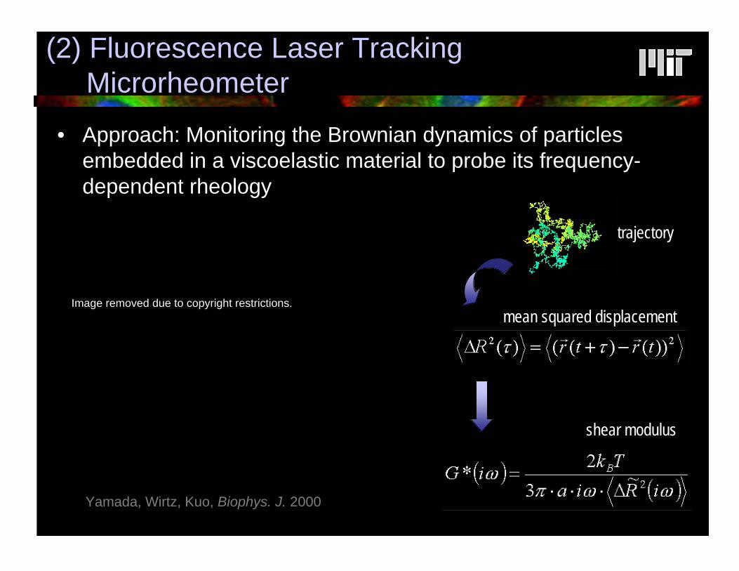
(2) Fluorescence Laser Tracking Microrheometer

• Approach: Monitoring the Brownian dynamics of particles embedded in a viscoelastic material to probe its frequency-dependent rheology

trajectory

Image removed due to copyright restrictions. mean squared displacement

shear modulus

Yamada, Wirtz, Kuo, Biophys. J. 2000

(2) Nanometer Resolution for the Bead’s Trajectory

Photons detected per measurement 103 104 105 106

Uncertainty on 0.033 0.010 0.003 0.001

Uncertainty on xc (nm) 12 4 1.2 0.4

xc

A B

σ = 0.5 µm

x

• Collecting enough light from a fluorescent bead is critical

Nanometer resolution ↔ 104 photons per measurement

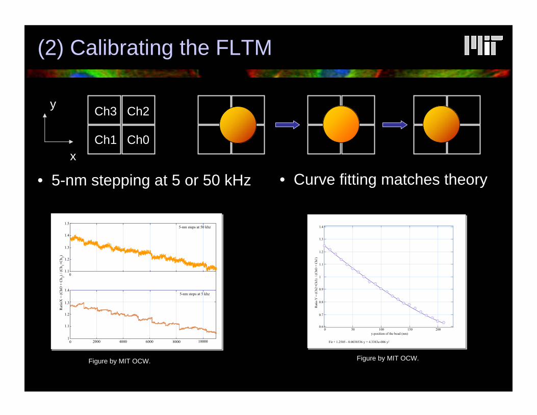
(2) Calibrating the FLTM

x

y Ch2Ch3

Ch0Ch1

• 5-nm stepping at 5 or 50 kHz • Curve fitting matches theory

1.5

1.4

1.4

1.3

1.3

1.2

1.2

1.1

1.1

0

0

2000 4000 6000 8000 10000 1

5-nm steps at 50 khz

5-nm steps at 5 khz

Rat

ioX

= (C

hO +

Ch 2 ) /

(Ch 1 +C

h 3 )

Figure by MIT OCW.

1.4

1.3

1.2

1.1

1

0.9

0.8

0.7

0.6 0 50 100 150 200

Fit + 1.2505 - 0.0038536 y + 4.3383e-006 y2

Rat

io Y

= (C

h2+C

h3)

/ (C

hO +

Ch1

)

y-position of the bead (nm)

Figure by MIT OCW.

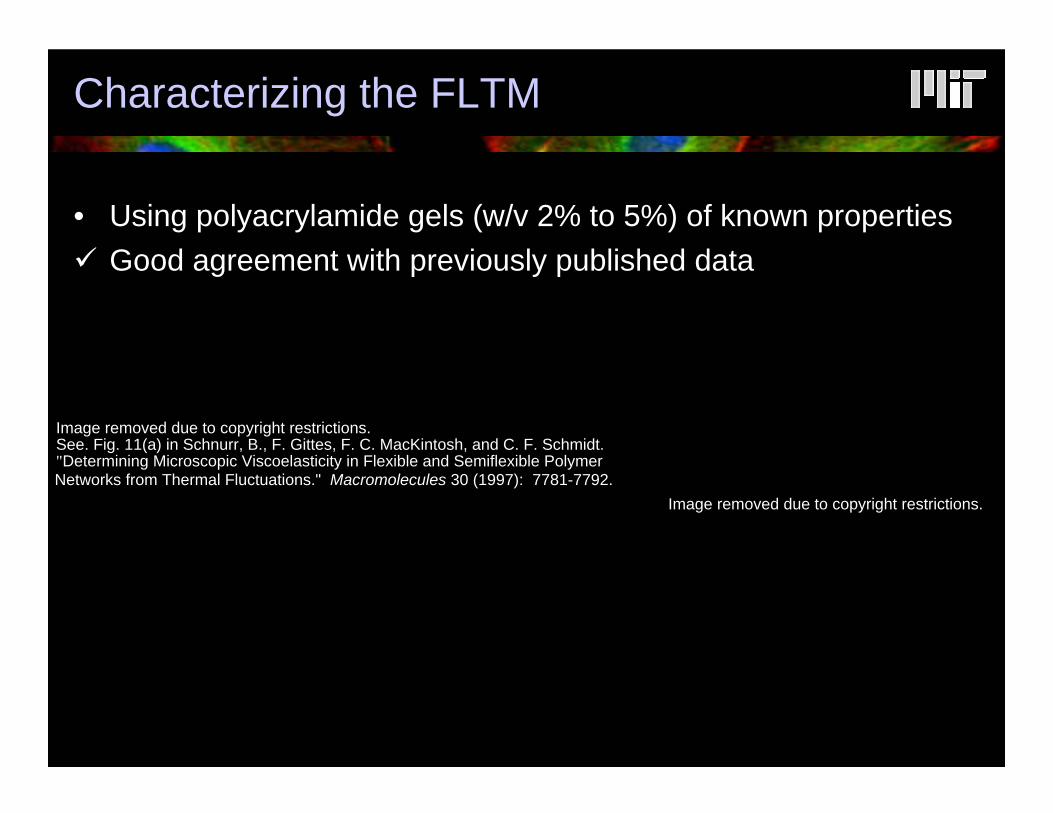
Characterizing the FLTM

• Using polyacrylamide gels (w/v 2% to 5%) of known properties 9 Good agreement with previously published data

Image removed due to copyright restrictions. See. Fig. 11(a) in Schnurr, B., F. Gittes, F. C. MacKintosh, and C. F. Schmidt. "Determining Microscopic Viscoelasticity in Flexible and Semiflexible Polymer Networks from Thermal Fluctuations." Macromolecules 30 (1997): 7781-7792.

Image removed due to copyright restrictions.

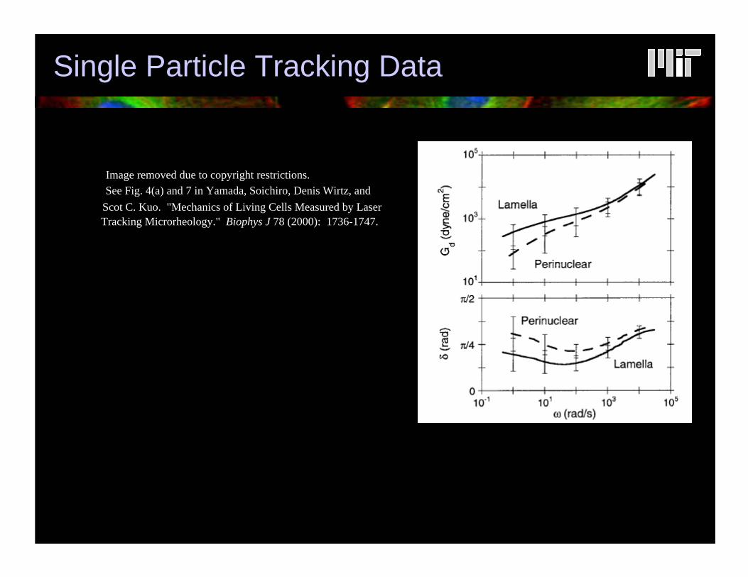
Image removed due to copyright restrictions.See Fig. 4(a) and 7 in Yamada, Soichiro, Denis Wirtz, and Scot C

Image removed due to copyright restrictions.��ics of Living Cells Measured by Laser Tracking MicrorheologySee Fig. 4(a) and 7 in Yamada, Soichiro, Denis Wirtz,

and Scot C. Kuo. "Mechanics of Living Cells Measured by Laser Tracking Microrheology." Biophys J 78 (2000): 1736-1747.

J 78 (2000): 1736-1747.

. Kuo. "Mechan." Biophys

Single Particle Tracking Data

Image removed due to copyright restrictions.�� See Fig. 4(a) and 7 in Yamada, Soichiro, Denis Wirtz, and

Scot C. Kuo. "Mechanics of Living Cells Measured by Laser Tracking Microrheology." Biophys J 78 (2000): 1736-1747.

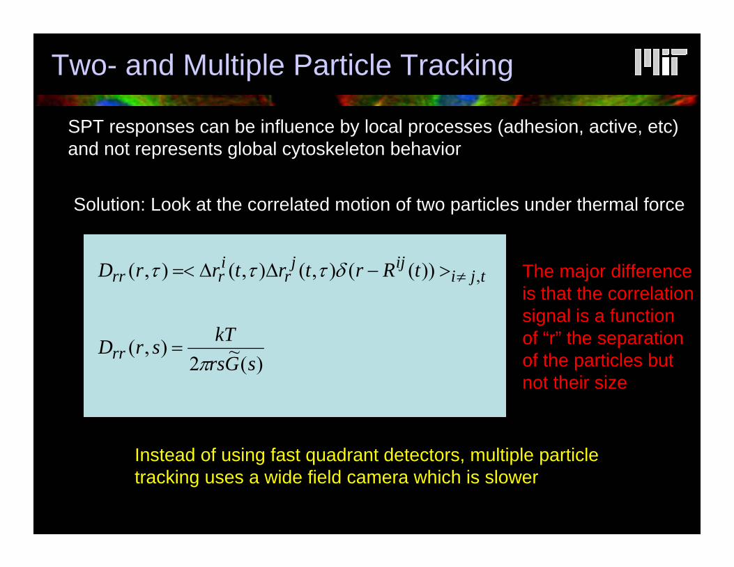
Two- and Multiple Particle Tracking

)( ~ 2),(

))((),(),(),( ,

sGrskT srD

tRrtrtrrD

rr

tjiijj

r i rrr

π

δτττ

=

>−∆∆=< ≠

Solution: Look at the correlated motion of two particles under thermal force

Instead of using fast quadrant detectors, multiple particle tracking uses a wide field camera which is slower

SPT responses can be influence by local processes (adhesion, active, etc) and not represents global cytoskeleton behavior

The major difference is that the correlation signal is a function of “r” the separation of the particles but not their size

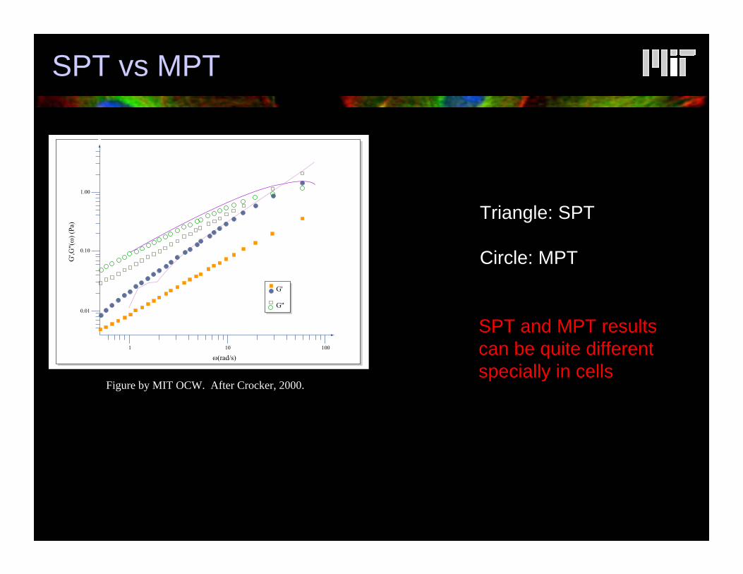
SPT vs MPT

Triangle: SPT

Circle: MPT

SPT and MPT results can be quite different specially in cells

Figure by MIT OCW. After Crocker, 2000.

1.00

0.10

0.01

1 10 100

G'

G"

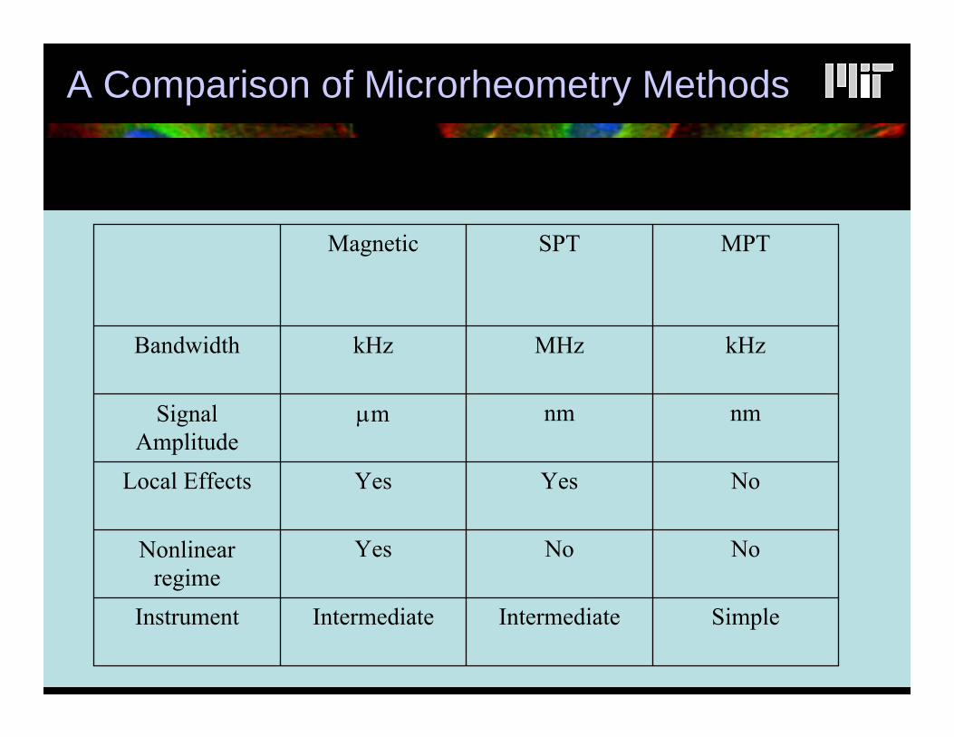
A Comparison of Microrheometry Methods

Magnetic SPT MPT

Bandwidth kHz MHz kHz

Signal Amplitude

µm nm nm

Local Effects Yes Yes No

Nonlinear regime

Yes No No

Instrument Intermediate Intermediate Simple