Gender Differences in Negotiation:

Evidence from Real Estate Transactions

Steffen Andersen Copenhagen Business School and CEPR

Julie Marx

Copenhagen Business School

Kasper Meisner Nielsen Copenhagen Business School and HKUST

Lise Vesterlund University of Pittsburgh & NBER

October 2018

Abstract

Proper assessment of the negotiated ‘item’ is essential in determining whether individuals secure different outcomes through negotiations. For example, evidence that negotiations lead to higher wages for men than women need not imply differences in negotiation ability but may reflect differences in outside options and in the assessed value of the employee-employer match. Investigating real estate negotiations, we study a market with detailed information on the value of the negotiated item. We find evidence that men secure better prices than women do when negotiating to buy and to sell property. However, this price difference declines substantially when we include better controls for the property’s value; and the difference is essentially eliminated when we control for unobserved heterogeneity in a sample of repeated sales. Intriguingly, the price difference is completely absent when we look at the sales prices individuals secure for property inherited from a deceased parent. This finding suggests that gender differences from real estate negotiations likely result from insufficient value assessment and from failure to properly control for the different property characteristics demanded by men and women. Provided appropriate controls, we find no evidence that men and women secure different prices when negotiating over real estate.

1

1. Introduction

This paper examines whether men and women secure different outcomes through negotiation. A

classic example of such differences is seen in the labor market, where gender differences in

initiating and engaging in negotiations are noted as contributing to the persistent gender wage

gap. For example, the seminal work of Babcock and Laschever (2003) shows in a survey of new

graduates that 57% of the men and only 7% of the women negotiated the initial compensation

offered to them.1 With an average gain from negotiation of 7.4%, this differential in initiating

negotiation is predicted to magnify over time and to result in a substantial wage difference in the

long run.2 Although negotiation in the labor market is of key concern, it is unfortunately a

market where it is challenging to examine gender differences in negotiation. In particular, the

researcher has difficulty assessing the value of the employee-employer match and the parties’

outside options. The difficulty associated with assessing the ‘value’ of the negotiated ‘item’ thus

challenges whether gender differences in outcomes necessarily result from differences in

willingness and ability to negotiate.

Gender differences in negotiation outcomes have also been examined for items that are more

easily assessed. For example, Ayres (1991, 1995) and Ayres and Siegelman (1995) report audit

studies related to cars, concluding that single women pay higher prices for the same car than do

single men. Similarly, Castillo, Petrie, Torero, and Vesterlund (2013) uncover gender differences

in bargaining outcomes for taxi rides, finding (as in Ayres, 1991, 1995; and Ayres and Siegelman,

1995) that statistical discrimination plays a central role in driving these differences. Note,

however, that audit studies primarily point to differential treatment of men and women. As

buyers are instructed on how to negotiate, audit studies do not demonstrate gender differences in

the ability and willingness to negotiate. List (2004) instead conducts an experiment in which

negotiations over sports cards are incentivized and free form. His study reveals that men secure

better prices than do women, and that the uncovered differences are consistent with statistical

discrimination. As the study was designed to capture differential treatment by dealers of non-

dealers it did not provide incentives that make it well suited for capturing gender differences in

negotiation.3

1 See also Babcock et al. (2003), Small, Gelfand, Babcock, and Gettman (2007), Bowles and McGinn (2008), Erikson and Sandberg (2012), Leibrandt and List (2015), and for reviews Azmat and Petrongolo (2014) and Stuhlmacher and Walters (1999). 2 These results have led to a push for women to lean-in and negotiate more (Sandberg, 2013). Exley, Niederle and Vesterlund (2016) however show that such a recommendation may be misguided in the presence of positive selection. 3 In particular gender differences in negotiation can only be evaluated among non-dealers and the design was such that non-dealers did not decide on whether to negotiate, nor did they have negotiation incentives that were likely to result in transactions (only 3% of negotiations led to a transaction).

2

The real estate market is potentially an attractive market when studying differences in

negotiation. Both men and women are actively engaged in the market; information on the

negotiated item is abundant; negotiations may have large financial implications; and individuals

are seen both as buyers and sellers in the market. Intriguingly, prior work has found that women

secure worse prices than do men in real estate negotiations. Examining data from the US,

Harding, Rosenthal, and Sirmans (2003) document substantial gender differences and conclude

that these differences in prices suggest “that women have less bargaining power than men,

consistent with audit findings by Ayres and Siegelman (1991, 1995) and Ayres (1995).”

Using real estate transactions from Denmark, we ask whether these results survive when

we introduce better controls for the value of the negotiated item. First, examining negotiation

outcomes of 337,685 real estate transactions of Danish properties from 1994 to 2013, we find

that single men secure better prices than do single women when they negotiate both to buy and

to sell property. However, this price difference is reduced when controlling for observable

characteristics of the property, and it is further reduced when using the tax-assessed value of the

property to control for characteristics that, while observable to the tax authorities, are

unobservable to us as researchers. Furthermore, the gender difference in prices is essentially

eliminated when looking at repeat sales of the same property and including property fixed

effects. The repeated sales analysis, which is a common approach in real estate economics,

effectively controls for time-invariant heterogeneity (e.g., location amenities) in properties by

including property fixed effects. These findings suggest that the evidence of gender differences

in real estate negotiations result from insufficient controls for the value of the negotiated item.

Second, to eliminate the possibility that price differences result from men and women

demanding different properties, and from our failure to control for these characteristics, we also

examine differences in sales prices secured for a “random” property. We find that the gender

difference in prices is completely absent when looking at the sales prices individuals secure for

property inherited from a deceased parent. The analysis of death sales imitates a natural

experiment in which properties are randomly assigned to sellers, and substantially reduces or

eliminates the possibility that seller characteristics influence the item that is being sold. It follows

that death sales provide us with an opportunity to estimate gender differences in transaction

prices that are driven by negotiation rather than by gender differences in preferences and

demand for property characteristics.

Our results suggest that initial evidence of gender differences from real estate negotiations

likely results from insufficient controls for value and failure to control for the different property

characteristics demanded by single men and single women. Provided with proper controls, we

3

find no evidence that transaction prices differ by gender when individuals negotiate over real

estate. Thus, our results demonstrate that proper assessment of the negotiated item is needed

when determining whether individuals secure different outcomes through negotiation. Further,

our study presents the real estate market as an institutional setting that effectively secures that

potential gender differences in negotiation do not affect outcomes.

The paper is organized as follows. Section 2 presents the data and descriptive statistics.

Section 3 outlines the hedonic model of property prices and explains how we estimate

negotiation outcomes in the real estate market. The emphasis is on securing proper controls for

the negotiated item when examining all transactions, and when examining only the properties for

which we observe repeat sales. Section 4 examines gender differences when we eliminate the

potential role gender differences in demand may have on the transaction price. That is, it

presents results from death sales where we restrict the sample to beneficiaries who sell an

inherited property. Section 5 offers concluding remarks.

2. Data and descriptive statistics

Our data cover all transactions of residential real estate in Denmark from 1994 to 2013, and

contain economic and personal information about buyers and sellers, as well as property

characteristics and transaction prices. We derive data from six sources made available through

Statistics Denmark:

1. Property transactions are from the Danish Tax and Customs Administration (SKAT).

SKAT receives the information from The Danish Gazette (Statstidende). Public announcement in

The Danish Gazette is part of the juridical registration of the transfer of ownership, which

ensures that we have access to accurate and reliable information on property transactions over

the sample period. The transaction data include the property price, transaction date, as well as

the property identification number used in the housing register described below.

2. Individual characteristics of houses are from the Housing Register (Bygnings- og

Boligregister, BBR), which has detailed information on all properties in Denmark. In addition to a

property identification number and property characteristics, the data contain the personal

identification numbers (CPR nummer) of the property owner at the end of each year. We identify

sellers as owners of a transacted property in the beginning of the year of the transaction, and

buyers as owners of the property at the end of the year.

4

3. Individual and family data are from the official Danish Civil Registration System (CPR

Registeret). These records include the individual’s personal identification number (CPR number),

gender, age, and marital history (marriage, divorce, and widowhood). We use these data to obtain

individual characteristics as well as civil status.

4. Income data are from the official records at the Danish Tax and Customs

Administration (SKAT). This dataset contains income information by CPR number for the

entire Danish population. The tax authorities receive this information directly from the relevant

sources: Employers withhold income tax and pay it directly to SKAT while informing SKAT

about the actual wages paid to their employees. The data from the tax authorities also contain an

assessment of house values, which forms the basis for the property value tax and the

municipality land tax. To facilitate the collection of property taxes, the Danish tax authorities

(SKAT) assess the value of properties by estimating the property value if it were to be sold. The

valuation takes into account factors such as local market conditions, an array of house

characteristics, and permissible alternative uses of the land. The assessment is carried out every

other year, and in years in which a house is not assessed by the tax authorities, the value is

regulated based on the growth in local house prices. The assessment is carried out at the

municipal level and incorporates factors that are unobserved in the data from the Housing

Register. These factors include access to recreational space (e.g., beach, forest, or lake); distance

to public transportation; and other amenities (e.g., schools).

5. Educational records are from the Danish Ministry of Education. All completed (formal

and informal) education levels are registered on a yearly basis.

6. Employment statuses are from Statistics Denmark’s IDA database. An individual’s

employment status is classified at the end of November each year. Individuals are classified as

employed when the majority of their personal income derives from paid employment, and as

self-employed when the majority of their personal income is from self-employment. Individuals

outside the labor market are classified as “retired” if the majority of their income is from private

or public pensions. Finally, individuals are classified as unemployed if they are neither employed

nor self-employed, and have not retired.

Collectively, these data sources allow us to assess transaction data, and link them to buyer

and seller characteristics. To correctly identify the agents involved in the transaction, we exclude

properties that are traded more than once within a year. To analyze the effect of gender on real

estate negotiations, we focus on transactions by single females and single males and require that

each household has an unchanging number of adult members (aged between 18 and 65 years)

5

over a two-year period around the time of the property transaction. This focus ensures that the

individuals engaged in a transaction do not change status from being single to being part of a

couple, or vice versa. We further restrict the sample to arm’s length transactions by excluding

transactions between family members. Finally, we focus our analysis on transactions of houses

and apartments and exclude, on account of poor controls and small samples, cottages, farms, and

condominiums. Our gross dataset includes 337,685 observations of real estate transactions in

Denmark from 1994 to 2013. Table 1 presents descriptive statistics on buyer and seller

characteristics, while Appendix A provides additional details on the sample selection and

definition of variables.

[Table 1 here]

Table 1 shows buyer and seller characteristics for all transactions, and for transactions

involving single women, single men, or couples among buyers and sellers, respectively. Around

65,000 (71,000) transactions, corresponding to 19% (21%) of all transactions, have a buyer

(seller) who is single. Among buyers, single women are older, have lower income, have greater

wealth, and are better educated, than are single men.4 The same contrast holds among sellers,

where these differences are slightly larger. The difference in individual characteristics of single

males and single females highlights the importance of controlling for individual characteristics

when assessing the effect of gender on realized real estate prices. Table 2 shows property

characteristics for all transactions, and transactions involving single women, single men, or

couples among buyers and sellers, respectively.

[Table 2 here]

A simple comparison of transaction prices, as shown in Table 2, reveals that single women

both buy and sell at higher prices than do single men. Panel A focuses on houses, and shows that

single women buy houses that cost DKK 175,600 (EUR 23,600) more than those bought by

single men. The difference in transaction prices implies that single women buy houses that are 17

percent more expensive than those bought by single men. When single women sell, the

transaction price is DKK 128,500 (EUR 17,200) higher than houses sold by single men. The

difference in transaction prices corresponds to a 10 percent gender difference in sales prices. A

4 Amounts in our study are in 2015 Danish kroner (DKK). One Euro equals 7.45 Danish kroner.

6

naïve interpretation of these differences is that single women are worse at negotiating: they pay

more when buying a property, and while also selling at a higher price, they are not as effective in

recapturing the higher price they paid when purchasing the property. The raw data suggest that,

when negotiating over real estate, single women leave DKK 47,100 (EUR 6,300) more on the

table than do single men. However, this difference in transaction prices may result from single

women and single men demanding different property characteristics, either because of

differences in financial constraints and other individual characteristics (Table 1), or because their

preferences for property characteristics differ. Potential differences in demand imply that we

must control for characteristics of the transacted property to uncover differences in negotiation,

rather than differences in demand. A closer look at Panel A of Table 2 reveals, however, that

gender differences in transaction prices do not correspond to substantial differences in

researcher observable house characteristics. Gender differences are small in easily observable

property characteristics that are likely to increase the transaction price, and are small relative to

the 17% and 10% gender difference in purchase and sale prices. When purchasing property, the

gender difference in interior size is less than 2 square meters (2%), equivalent to 0.04 more

rooms (1%), and less than 0.03 more bathrooms (3%). When selling a property, gender

differences are slightly larger. In comparing the sales and purchase side we can thus assess the

potential role of property characteristics on prices. Finding relatively larger gender differences in

property characteristics and relatively smaller gender differences in transaction prices on the sales

than on the purchase side suggests that the gender difference in prices are unlikely to be fully

accounted for by property characteristics that are observable in the Housing Register.

The Housing Register, however, does not capture all characteristics of a transacted

property. In particular, the Danish tax authorities have more detailed information available when

assessing the value of a property (e.g., local market amenities and conditions, permissible

alternative uses of the land). We may, in including the tax authorities’ property assessment, better

control for the value of the property characteristics that are not captured in the raw

characteristics given in the Housing Register. Using the tax assessment of the property in the

year prior to the transaction, we find that transactions involving single women are for properties

that have systematically higher assessed value than for transactions involving single men. When

purchasing a property, the difference of DKK 112,200 (EUR 15,000) in the assessed value

corresponds to almost two-thirds of the observed gender difference in transaction prices. When

selling, the difference of DKK 96,900 (EUR 13,000) in assessed value corresponds to three-

quarters of the gender difference in transaction prices. While using the tax authorities’ assessed

property value as the benchmark reduces the gender difference in transaction prices substantially,

7

an economically large difference in transactions prices still remains. Single women buy properties

priced DKK 63,400 (EUR 8,500) above the assessed value relative to single men but only sell

properties at prices DKK 31,600 (EUR 4,200) above the assessed value relative to single men.

The triple difference of DKK 31,800 (EUR 4,300) suggests that single women leave 2 to 3

percent of the property value on the table when they negotiate over real estate.

Panel B, which focuses on apartments, provides additional insights into the potential

gender differences in negotiations. The market for apartments is more liquid and transparent

than the market for houses, making it easier for market participants, as well as researchers, to

estimate the market value by finding the price from a recent transaction involving a comparable

apartment. In this more liquid and transparent market we continue to find gender differences in

prices.5 Panel B shows that single women buy apartments at prices that are DKK 120,700 (EUR

16,200) higher than do single men, and sell apartments at DKK 99,700 (EUR 13,400) higher

prices. The difference in transaction prices of DKK 21,000 (EUR 2,800) remains consistent with

single women performing worse in real estate negotiations. Again we notice that observed

property characteristics can explain a relatively small part of the difference in price. Relative to

men, women buy and sell slightly larger apartments. Similarly, using the tax authorities’

assessment of value, we again note that part of the difference likely results from unobservable

differences in the properties demanded by single men and women. Single women buy

apartments priced DKK 36,900 (EUR 5,000) above the assessed value of those bought by single

men, but only sell properties at prices DKK 20,100 (EUR 2,700) above the assessed value of

those sold by single men. The triple difference suggests that single women leave 1 to 2 percent of

the apartments’ value on the table, relative to single men.

The main takeaway from Table 2 is thus that gender differences exist in transaction prices.

Single women buy at higher prices than those at which they sell, relative to single men. Although

part of the gender difference in prices appears to be explained by gender differences in demand

for observable and (to us) unobservable property characteristics, differences in transaction prices

may also result from gender differences in negotiation. The identification of potential gender

differences in negotiation, whether as a result of differences in bargaining power, ability, or

frequency of initiating a negotiation, thus warrants a more careful analysis of our sample of real

estate transactions.

5 Past research finds evidence that women fare worse in negotiations that involve more ambiguity (see, e.g., Bowles and McGinn, 2008; Leibbrandt and List, 2015).

8

3. Real estate negotiation

For heterogeneous goods like real estate, the market is thin and no observed market-clearing

price exists. Facilitating negotiation, real estate transactions arise when a buyer’s willingness to

pay is higher than the seller’s reservation price. Thus the observed transaction price will not only

depend on the characteristics of the transacted property, but also on negotiation between buyers

and sellers.

One approach to uncovering gender differences in negotiation outcomes is to examine a

simple hedonic model of prices on property characteristics. As expected from the raw means the

simple hedonic approach reveals that single women fare worse than men when negotiating over

property. Women leave more money on the table than men when negotiating over houses or

apartments.6

However, as shown by Harding, Rosenthal, and Sirmans (2003) (henceforth HRS) the

simple hedonic model fails to control for differences in demand for property characteristics.

That is, the estimated gender effect includes both differences in negotiation and in demand. To

examine whether gender differences in the realized transaction prices result from differences in

negotiation or from men and women demanding different types of properties, we therefore

follow the approach of HRS and assume trading symmetry in both negotiation ability and

demand. The assumption implies that the negotiation ability is symmetric and independent of

whether the individual is a buyer or a seller.7 This symmetry assumption helps separate

negotiation from demand effect by adding differences in seller-buyer characteristics and sums of

seller-buyer characteristics to a standard hedonic model of house prices. The main HRS model

for estimating the gender difference in negotiation is specified in Equation (1), where the

dependent variable is the log price, yijt, of house (or apartment) i in municipality j in year t:

���� = �� + �� + ���� + �������� − ��

���� + ����

���� + �����

� + ����. (1)

Where Xit is a vector of observed property characteristics for property i at time t, and Disell

and Dibuy are vectors of seller and buyer characteristics. The coefficient � on the sums of the

seller-buyer characteristics is the estimated demand effect, whereas the coefficient � on the

6 Appendix Table E1 reveals results from the simple hedonic model and shows that the raw gender difference is somewhat larger in a simple hedonic regression that does not control for differences in demand (3%, rather than 2.1%). However, the response to improved controls is similar, and the gender difference is similarly eliminated when properly controlling for the value of the negotiated property. 7 See Appendix B for a description of the HRS model.

9

differences in seller-buyer characteristics is the estimated negotiation effect. To control for

general trends and seasonality in house prices, we further include year, quarter, and municipality

fixed effects (αj and αt, respectively).

[Table 3 here]

We begin by directly using the HRS specification. The associated results are shown in Table 3,

first separately for houses and apartments, and then when pooling the two.8 For the three

models, we show, in the first column, the estimated negotiation effects, �; in the second column,

the estimated demand effects, �; and in the third column, other controls, including the effect for

variables that only refer to buyers (out-of-town and first-time home buyers), where the demand

and negotiation effects cannot be separated. Note that a positive negotiation coefficient reflects

greater bargaining power, in the sense that the seller sells for more and the buyer pays less, and

that a positive demand effect implies greater willingness to pay.

We see in columns 2 and 5 of Table 3 that the price of the demanded property, whether for

houses or apartments, tends to increase with income, education, and being self-employed;

however, as seen in columns 1 and 4, such characteristics are also correlated with securing worse

outcomes when negotiating over real estate. These results replicate that of HRS, who argue that

this inverse relationship between negotiation and income may reflect the effect of diminishing

marginal utility of income.9

If gender differences in negotiation help explain the observed variation in transaction prices

in Table 2, we expect a negative coefficient on the indicator for a single female. Consistently,

Column 1 in Table 3 shows that single women leave 2.0% on the table when trading houses.10

Column 4 in Table 3, in contrast, shows that women only leave 0.2% on the table when trading

apartments. As noted above the market for apartments is more liquid and transparent and leaves

less room for negotiation, thus the estimated coefficients on negotiation are expected to be

smaller for apartments. In columns 7, 8, and 9, we confirm these results when combining houses

and apartments into one specification and when including an interaction term between single

8 See Appendix Table D4 for the distribution of trades between single females, single males, and couples. For brevity, we do not report the estimated coefficients on property characteristics throughout the analysis. Tables with estimated coefficients on property characteristics are available from the authors upon on request. 9 Augmenting the HRS model to include wealth does not alter the results; see Appendix Table C1. For comparability, we maintain the HRS specification. 10 The effect does not depend of the state of the market. Running a regression with year-gender interactions shows a persistent difference over 20 years, a period that includes both the housing market bubble and bust.

10

woman and an indicator for apartments. We find a gender difference of -2.1% on prices for

houses, and a gender difference of -0.7% for apartments.That is we replicate earlier evidence that

single women fare worse than single men when negotiating over real estate. 11

We noted in Table 2 that a large fraction of the gender difference in property prices may

be driven by unobserved heterogeneity in the transacted property. To further our understanding

of potential gender differences in negotiation, we next aim to better control for unobserved

heterogeneity. Specifically, we further control for the tax authority’s assessment of the property

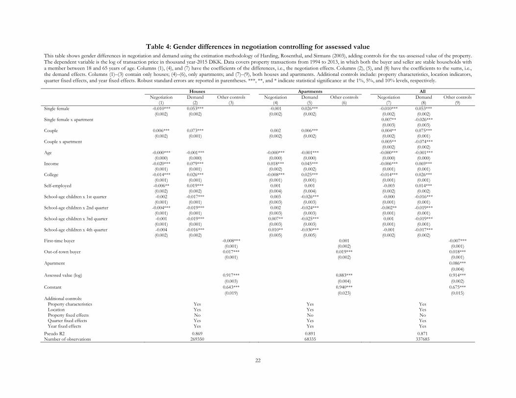
value in the year prior to the transaction. Table 4 includes the log of the assessed value of the

property. Looking at the specification for houses, we see in Column 3 that a 10% increase in the

assessed value of the property is associated with a 9.2% higher transaction price, after controlling

for time-trends and observable property characteristics. Thus, heterogeneity in property values

that are assessed by the tax authorities are similarly valued when the properties are transacted.

This finding indicates that the assessed value helps control for the value of the negotiated item,

and that the value, in turn, helps us identify gender differences in negotiation.

We see for houses in Column 1 of Table 4 that half of the estimated gender difference

disappears when we control for the tax authorities’ value assessment of house characteristics that

are observable to them.12 Comparing the results for the pooled sample in Column 7 of tables 3

and 4, we see that more than half of the gender difference for houses disappears. The gender

difference in Table 3 is estimated to be -2.1% for houses, compared to -1.0% when we control

for the assessed value. For apartments, the estimated gender difference in Column 7 is reduced

from -0.7% to -0.3%.13 This reduction in the coefficient on gender demonstrates that our initial

evidence of gender differences in negotiation partially results from property characteristics and

the value of the negotiated item not being properly controlled.

[Table 4 here]

Results from tables 3 and 4 highlight that the main caveat to estimating gender differences

in negotiation is whether we have properly control for property characteristics and thus for

11 These are robust to controls for financial wealth; see Appendix Table C1. Our result for houses corresponds to those of HRS, who find a gender difference of around 4% for American house transactions. 12 To examine whether the unobserved property characteristics are correlated with ownership length due to, for example, gender differences in the ability or interest in maintaining the property, we also control for the length of the seller’s ownership as well as the interaction between length of ownership and gender (Appendix Table F1). Although transaction prices, as expected, decline with ownership, we find no evidence of gender differences being driven by ownership length. 13 Results are similar when controlling for wealth in Appendix Table C2.

11

potential gender differences in the demands. While the hedonic model includes many observable

property characteristics, one might be concerned about whether unobserved property

characteristics (e.g., property quality) correlate with potential gender differences in demand. A

common approach for capturing unobservable property characteristics is to conduct a repeated

sales analysis that includes property fixed effects to control for time-invariant heterogeneity (e.g.,

location amenities) in properties. When the specification includes property fixed effects, gender

differences are estimated using variation in transaction prices of the same property across time,

which ensures that the estimated gender difference is not driven by preferences for specific

locations or other unobserved time-invariant house characteristics. Table 5 shows the results

using a sample of the 71,417 property transactions of houses and apartments that are traded

more than once between 1994 and 2013.14

[Table 5 here]

The results in Table 5 are striking. When we control for time-invariant heterogeneity in

properties by including property fixed effects, the demand effect remains unchanged while the

gender differences in negotiation completely disappear.15 Thus, no differences exist in the

estimated negotiation effect of single men and of single women in the Danish real estate market

as long as we properly control for differences in property quality. We find no gender difference

for apartments or houses, suggesting that the estimated gender differences in negotiation in

tables 2, 3, and 4 are artifacts of the econometric specification, as opposed to underlying

differences in negotiation driven by gender. We also note that the coefficient on the single

female indicator is quite precisely estimated to be (close to) 0.16 Thus, the coefficients on the

single female indicator do not become statistically insignificant because of large standard errors.

Standard errors in Table 5 are of the same order of magnitude as in the baseline results in Table

3.

14 See Appendix tables D1 and D2 for the repeat sales equivalents of tables 1 and 2. See also Appendix Table F2 for Table 5 without property fixed effects. 15 Controlling for wealth provides similar results; see Table C3. 16 As seen in Appendix Table E1, the results are similar in a simple hedonic model that does not control for differences in demand. For example, when accounting for differences in demand, we found that property assessment controls decrease the gender gap for houses from 2.1% to 1.0%, and that the gap is further reduced to 0.0% when looking at repeat sales. Absent controls for differences in demand, the standard hedonic model shows that property assessment decreases the gender gap from 3.0% to 1.2% and that restriction to repeat sales further decreases it to an insignificant -0.3%.

12

Figure 1 summarizes the findings of tables 3 to 5 by plotting the estimated gender

difference in negotiations as well as the 95 percent confidence interval. The figure indicates that

the estimated gender differences diminish when we include the assessed house value as a control,

and disappear when we include property fixed effects to control for unobserved heterogeneity in

house quality. To further validate the finding of no gender differences in outcomes in the real

estate market, we next use a more direct approach to secure that differences in demand do not

influence the results. We perform an out-of-sample test of gender differences in property prices

in a natural experiment where individuals are selling a close-to-random property. The natural

experiment entails exclusively looking at death sales in which inherited properties are sold by the

child of a deceased parent.

4. Death sales

In the previous section, we find no gender differences in negotiation when we control for time-

invariant, but unobserved, characteristics of houses or apartments. To convincingly rule out

gender differences in negotiation in the real estate market, we next employ a research design that

imitates a natural experiment in which properties are randomly assigned to sellers. We thereby

eliminate potential differences in demand. Death sales thus help us estimate gender differences in

the realized transaction prices that are more likely to be driven by negotiation.

To identify property owners who have died, we use information from the Danish Cause-

of-Death Register at the Danish National Board of Health (Sundhedsstyrelsen). The source of these

data is the official death certificates issued by a doctor immediately after a death. Danish law

further obliges the relatives to report the death to their local funeral authority within two days.

The funeral authority formally notifies relevant government agencies, including the Central

Office for Personal Registration (CPR Registeret) and the probate court (Skifteretten), which

supervises the process that transfers legal title of property from the decedent’s estate to her

beneficiaries. The probate court posts a notice in The Danish Gazette (Statstidende) to advertise

for creditors, who in turn have 8 weeks to report their claims on the estate. Following the notice

period, assets are either liquidated or valued by the probate court with the purposes of

establishing the net worth of the estate, meeting liabilities, and incurring the estate tax. At the

closing of the estate, the residual is paid out to the beneficiaries. According to the Association of

Danish Estate Lawyers, estates take, on average, 9 months to resolve. During this period,

beneficiaries are entitled to appoint a real estate agent to secure the sale of the property.

13

We restrict the sample to properties sold by the beneficiary of a deceased owner. More

specifically, we identify in our sample 13,953 houses and apartments, for which the owner is

single or widowed, has only one child, and dies. The sample is secured by linking owners to their

beneficiaries using the data from the Civil Registration System, which allows us to link parents

and children using personal identification numbers (CPR number). To ensure that the beneficiary

has decision power over the estate and, therefore, approves the sale of the inherited property, we

focus our test on inheritance cases with a single beneficiary. This focus simplifies the analysis, as

the beneficiary is either single male, single female, or a married couple.17

The advantage of analyzing death sales is that the gender of the beneficiary is likely to be

determined by nature.18 Table 6 shows property characteristics for all death sales, and for

beneficiaries who are single men or single women.

[ Table 6 here]

Table 6 shows that the characteristics of inherited houses are close to the characteristics of

all houses in our sample. The main difference arises from the fact that death sales consist of

properties owned by households comprised of a single member. Naturally, such properties are

smaller and older than the average property. We note that small differences exist in the property

characteristics for single male and single female beneficiaries. Single women beneficiaries tend to

sell their inherited properties at higher prices than do single male beneficiaries, although property

characteristics, as summarized by the tax authorities’ assessed value of the property, explain a

large part of this difference. If anything, the descriptive statistics do not support gender

differences in negotiation in favor of men.

To estimate gender differences in negotiation in the death sales sample, we use an

econometric specification similar to Equation (1). Instead of including seller-buyer differences

and sums, we include ‘beneficiary-seller’-buyer differences (Disell – Di

buy) and ‘deceased-owner’-

buyer sums (Disell + Di

buy). The coefficient on ‘deceased-owner’-buyer sums, γ, controls for the

demand effect, which is related to the choices of the deceased owner. The coefficient on the

‘beneficary-seller’-buyer differences is the negotiation effect, δ, and relates to the seller

beneficiary, who is in charge of the negotiation:

17 As in the main analysis, we only include to arm’s-length transactions, by excluding transactions between family members. Andersen and Nielsen (2017) show that more than 90% of all inherited houses end up being sold at arm’s length. Thus, the potential bias resulting from transfers of ownership within the family is likely to be small. 18 Over 95 percent of beneficiaries in our death sample are born prior to 1980, before current techniques to identify the gender of children were widespread. Moreover, no evidence exists, that we are aware of, for a “missing women” problem (Sen, 1992) in Denmark.

14

���� = �� + �� + ���� + �������� − ��

���� + ����

��� + �����

� + ���� . (2)

Table 7 presents results from estimating Equation (2) in the death-sales sample.

[ Table 7 here]

In Column 1 of Table 7, we find a small negative, but statistically insignificant, effect of

female sellers on house prices. The sale price is increasing with beneficiary age, income, and

education, but does not depend on the gender of the seller. Again, the coefficient on the assessed

value of the property is economically meaningful, showing a one-to-one correspondence

between the assessed value and the transaction price. In Column 4 of Table 7, we find a positive,

but statistically insignificant, effect of female sellers on apartment prices. Columns 7, 8, and 9

confirm these results. Results are also robust to controlling for wealth; see Appendix Table C4.

We further note that the specification, despite the small sample size, does not lack power.

Almost all of the seller characteristics (e.g., couple indicator, age, income, and education) are

both statistically and economically significant. Gender, on the other hand, is statistically

insignificant.

Results from the death sale analysis bolster our finding that gender differences in

negotiation in the real estate market disappear once we control for unobserved heterogeneity in

housing quality. Women and men realize the same value when they sell property they inherit

from their deceased parents. Eliminating the possibility that seller characteristics are related to

property characteristics, we find no gender difference in realized property prices.

5. Conclusion

In this study, we examine whether men and women secure different outcomes through

negotiation. We examine negotiation in the market for residential real estate to secure proper

assessment of the value of the negotiated item. Our preliminary analysis uncovers a large gender

difference in negotiation that disappears when we adequately control for heterogeneity in

housing quality. At first glance, females appear to realize worse prices when they buy or sell

property. Women demanding property characteristics with higher value assessments explains the

difference in property prices: this factor results in higher purchase and sales prices for single

women than for single men. Our initial finding that females leave 2.1% on the table when they

negotiate declines to 1.0% when we use the tax authority’s assessment of property value to

control for unobserved heterogeneity. When we further focus on the subset of properties with

repeated sales in our data, for which we can control for time-invariant heterogeneity in quality

15

(e.g., location) by including property fixed effects, the gender difference disappears. We finally

confirm these findings using a natural experiment in which beneficiaries are selling inherited

properties. We find that single male and single female beneficiaries realize the same sales prices

when they are selling inherited properties. This result effectively rules out the possibility that the

estimated gender difference is confounded by differences in demand for housing. We conclude,

in contrast to prior work, that men and women secure the same outcomes when negotiating over

real estate. Our results demonstrate how failure to properly control for the value of the

negotiated item may lead to misguided inference on differences in negotiation.

Real estate negotiations differ from other negotiations for many reasons, and the frequently

documented evidence on gender differences in negotiations suggests that our results do not

apply generally.19 What the results do suggest is that the institutions surrounding real estate

negotiations are such that they effectively overcome potential gender differences in negotiations.

As such, the real estate market may shed light on what is needed to overcome such differences in

other markets.

19 Bowles, Babcock, and McGinn (2005) point to the gender gap in negotiation depending on the constraints and triggers of the particular negotiation.

16

References

Andersen, S., and K. M. Nielsen. 2017. Fire sales and house prices: Evidence from estate sales due

to sudden death. Management Science 63: 201–212. https://doi.org/10.1287/mnsc.2015.2292

Ayres, I. 1991. Fair driving: Gender and race discrimination in retail car negotiations. Harvard

Law Review 104: 817-872. https://doi.org/10.2307/1341506

Ayres, I. 1995. Further evidence of discrimination in new car negotiations and estimates of its

cause. Michigan Law Review 94: 109-147. https://doi.org/10.2307/1289861

Ayres, I., and P. Siegelman. 1995. Race and gender discrimination in bargaining for a new car.

The American Economic Review 85(3): 304–321.

Azmat, G. and B. Petrongolo. 2014. Gender and the labor market: What have we learned from

field and lab experiments?" Labour Economics, 30: 32-40.

Babcock, L., and S. Laschever. 2003. Women don't ask: Negotiation and the gender divide.

Princeton, NJ: Princeton University Press.

Babcock, L., S. Laschever, M. Gelfand, and D. Small. 2003. Nice girls don’t ask. Harvard Business

Review 81: 14–16.

Bowles, H. R., and K. L. McGinn. 2008. Gender in job negotiations: A two-level game.

Negotiation Journal 24(4): 393–410.

Bowles, H. R., L. Babcock, and K. L. McGinn. 2005. Constraints and triggers: Situational

mechanics of gender in negotiation. Journal of Personality and Social Psychology 89(6): 951–965.

Castillo, M., R. Petrie, M. Torero, and L. Vesterlund. 2013. Gender differences in bargaining

outcomes: A field experiment on discrimination. Journal of Public Economics 99: 35–48.

https://doi.org/10.1016/j.jpubeco.2012.12.006

Eriksson, Karin Hederos, and Anna Sandberg. 2012. Gender Differences in Initiation of

Negotiation: Does the Gender of the Negotiation Counterpart Matter? Negotiation Journal

28(4): 407-428.

Exley, C., M. Niederle, and L. Vesterlund. 2016. Knowing When to Ask: The Cost of Leaning

In. NBER Working Paper No. 22961

Harding, J.P., S.S. Rosenthal, and C.F. Sirmans. 2003. Estimating bargaining power in the market

for existing homes. Review of Economics and Statistics 85:178–188.

17

Leibbrandt, A., and J. A. List. 2015. Do women avoid salary negotiations? Evidence from a large-

scale natural field experiment. Management Science 61(9): 2016–2024.

List, J. 2004. The nature and extent of discrimination in the marketplace: Evidence from the

field, The Quarterly Journal of Economics 119 (1): 49–89.

Sandberg, Sheryl. 2013. Lean in: Women, work, and the will to lead. New York : Alfred A.

Knopf.

Sen, A. 1992. Missing women. BMJ 304: 587–588.

Small, D.A., M. Gelfand, L. Babcock, and H. Gettman. 2007. Who goes to the bargaining table?

The influence of gender and framing on the initiation of negotiation. Journal of Personality and

Social Psychology 93: 600–613. https://doi.org/10.1037/0022-3514.93.4.600

Stuhlmacher, A. F., and A.E. Walters. (1999). Gender differences in negotiation outcome: A

meta-analysis. Personnel Psychology, 52, 653-677.

18

Figure 1: Summary of results

This figure plots the point estimates and 95-percent confidence intervals of female negotiation across Table 3 to Table 5.

19

Table 1: Buyer and seller characteristics This table shows mean characteristics of buyers and sellers in 337,685 property transactions from 1994 to 2013, in which both buyers and sellers are between 18 and 65 years of age and did not experience a change in the composition of adult household members around the time of transaction. Households consist of one or two adults living together and the number of children living with them. A household takes part in a transaction if at least one adult in the household buys or sells property. Buyers are identified as the owners of the property the year after the transaction, while sellers are identified as the owners of the property, registered January 1, in the year of the transaction. We take household characteristics from December 31 in the year before the transaction year. Age is the mean age of the adult household members. Income and net wealth are household totals in 2015 prices, winsorized at 1 percent in both ends, and presented in millions Danish kroner. College is the share of adult household members with a college degree. Self-employed is the share of adult household members that are self-employed. All shares take values 0, 0.5, or 1. School-age children is a dummy for having children between 5 and 15 years old (the children do not necessarily live in the household). First-time buyer is an indicator on no member of the household previously having owned real estate. Out-of-town buyer is an indicator on the household purchasing property in a municipality they did not previously live in. Standard deviations are presented in parentheses for non-indicator variables. t-statistics are in brackets. *** indicates significance at the 1% level. See Appendix Table D3 for differences in indicator variables.

Buyers Sellers

All Single

women (1)

Single men (2)

Difference (1)-(2)

All Single

women (3)

Single men (4)

Difference (3)-(4)

Age (38.830) (41.86)0 (36.66)0 -0[5.20***0] (43.67) (49.46) (43.46) 0-[6.01***]

(11.36)0 (12.21)0 (11.62)0 -[55.4]***00 (11.82) (11.69) (12.19) -[67.21]***

Income (million DKK) 0.370) 0.350) 0.370) -0.02***0] 0.370) 0.340) 0.380) -0.04***0]

(0.20) 0 (0.20) 0 (0.22) 0 [-10.85] ***0 (0.19) 0 (0.18) 0 (0.22) 0 [-26.02] ***0

Net wealth (million DKK) 0.280) 0.480) 0.310) 0.17***0] 0.390) 0.780) 0.520) 0.25***0]

(0.87) 0 (1.08) 0 (0.96) 0 [21.08] ***0 (0.98) 0 (1.23) 0 (1.19) 0 [27.84] ***0

College 0(0.280) 0(0.34)0 0(0.200) 0-[0.14***0] 0(0.25) 0(0.27) 0(0.18) 0-[0.09***]

-[40.65]***0

-[28.69]***

Self-employed 0(0.040) 0(0.03)0 0(0.030) 0-[0.00***0] 0(0.04) 0(0.03) 0(0.04) 0[-0.01***]

0[-1.28]***0

0[-9.98]***

School-age children 0(0.280) 0(0.18)0 0(0.140) 0-[0.04***0] 0(0.30) 0(0.14) 0(0.19) 0[-0.05***]

-[12.39]0***

[-17.62]***

First-time buyer 0.300) 0.400) 0.500) -0.10***0]

[-25.41]***0

Out-of-town buyer 0.450) 0.400) 0.390) 0.00***0]

[0.97]***0

N 337,685 28,720 36,232

337,685 35,007 36,413

20

Table 2: Property characteristics This table shows characteristics of property transactions from 1994 to 2013, separately for houses and apartments. Price is the realized sales price, and assessed value is the assessed value of the property from the Danish tax authorities prior to the sales. Both prices and assessed value are measured in thousand year-2015 DKK. One Euro equals 7.45 DKK. Interior size and Lot size are measured in square meters. House age and building age are measured in years. Rooms and bathrooms are count variables. Rural indicates a rural area. Standard deviations are presented in parentheses for non-indicator variables. t-statistics are in brackets. *** and **

indicate significance at the 1% and 5% levels, respectively.

Buyers Sellers

All

Single women

(1)

Single men (2)

Difference (1)-(2)

Single women

(3)

Single men (4)

Difference (3)-(4)

A. Houses

Number of transactions 269,350) 16,322) 19,676)

25,449) 25,275)

Price (1,000 DKK) (1514.08)0 (1185.41)0 (1009.83)0 -[175.58***] (1365.16)0 (1236.70)0 -[128.46***]

(1097.75)0 0(900.89)0 0(912.03)0 0-[18.28]*** (1049.74)0 (1018.74)0 0-[13.98]***

Assessed value (1,000 DKK) (1213.08)0 0(973.42)0 0(861.24)0 -[112.17***] (1149.97)0 (1053.08)0 0-[96.89***]

0(834.63)0 0(702.03)0 0(686.52)0 0-[15.28]*** 0(840.28)0 0(791.43)0 0-[13.37]***

Interior size (m2) 0(121.46)0 0(100.81)0 00(99.47)0 -00[1.34***] 0(116.32)0 0(112.62)0 00-[3.69***]

00(45.89)0 00(36.72)0 00((38.00)0 00-[3.37]*** 00(45.44)0 00(45.68)0 00-[9.12]***

Lot size (m2) (1030.20)0 0(794.18)0 0(970.11)0 [-175.93***] (1004.06)0 (1087.06)0 0[-83.00***]

(2319.69)0 (1137.47)0 (1440.14)0 0[-12.67]*** (1504.45)0 (4290.55)0 00[-2.91]***

House age (years) 00(45.01)0 00(53.05)0 00(56.92)0 00[-3.86***] 00(50.68)0 00(52.21)0 00[-1.53***]

00(35.16)0 00(40.78)0 00(41.15)0 00[-8.90]*** 00(36.64)0 00(39.26)0 00[-4.54]***

Rooms (#) 000(4.42)0 000(3.82)0 000(3.78)0 00-[0.04***] 000(4.28)0 000(4.15)0 00-[0.12***]

000(1.33)0 000(1.15)0 000(1.22)0 00-[3.09]*** 000(1.34)0 000(1.34)0 0-[10.26]***

Bathrooms (#) 000(1.38)0 000(1.18)0 000(1.16)0 00-[0.03***] 000(1.32)0 000(1.28)0 00-[0.04***]

000(0.56)0 000(0.44)0 000(0.44)0 00-[5.66]*** 000(0.55)0 000(0.53)0 00-[8.66]***

Rural 000(0.31)0 000(0.31)0 000(0.42)0 00[-0.11***] 000(0.32)0 000(0.38)0 00[-0.06***]

0[-22.15]***

0[-13.23]***

B. Apartments

Number of transactions 68,335) (12,398) 16,556) 9,558) 11,138)

Price (1,000 DKK) (1331.11)0 (1207.52)0 (1086.87)0 -[120.65***] (1225.01)0 (1125.28)0 0-[99.73***]

0(897.87)0 0(755.11)0 0(701.23)0 0-[14.02]*** 0(793.71)0 0(763.58)0 00-[9.20]***

Assessed value (1,000 DKK) (1082.95)0 0(976.23)0 0(892.46)0 0-[83.77***] (1001.14)0 0(921.57)0 0-[79.57***]

0(751.09)0 0(643.79)0 0(597.12)0 0-[11.42]*** 0(679.38)0 0(648.33)0 00-[8.61]***

Interior size (m2) 00(76.43)0 00(71.91)0 00(69.02)0 00-[2.88***] 00(71.51)0 00(68.31)0 00-[3.21***]

00(29.61)0 00(22.85)0 00(23.55)0 0-[10.45]*** 00(26.63)0 00(27.24)0 00-[8.53]***

Building age (years) 00(63.55)0 00(61.61)0 00(61.47)0 00-[0.14]*** 00(63.89)0 00(63.34)0 00-[0.55***]

00(37.13)0 00(36.63)0 00(36.20)0 00-[0.31]*** 00(36.36)0 00(36.71)0 00-[1.08]***

Rooms (#) 000(2.67)0 000(2.52)0 000(2.38)0 00-[0.14***] 000(2.49)0 000(2.35)0 00-[0.14***]

000(1.06)0 000(0.89)0 000(0.89)0 0-[13.44]*** 000(1.00)0 000(0.98)0 0-[10.49]***

Bathrooms (#) 000(1.04)0 000(1.02)0 000(1.01)0 00-[0.01***] 000(1.03)0 000(1.02)0 00-[0.01***]

000(0.23)0 000(0.18)0 000(0.16)0 00-[4.41]*** 000((0.2)0 000(0.19)0 00-[2.82]***

Rural 000(0.02)0 000(0.01)0 000(0.01)0 00-[0.00]*** 000(0.01)0 000(0.01)0 00-[0.00]***

00[-0.45]*** 00-[1.20]***

21

Table 3: Gender differences in negotiation This table shows gender differences in negotiation and demand using the estimation methodology of Harding, Rosenthal, and Sirmans (2003). The dependent variable is the log of transaction price in thousand year-2015 DKK. Data covers property transactions from 1994 to 2013, in which both the buyer and seller are stable households with a member between 18 and 65 years of age. Columns (1), (4), and (7) have the coefficients to the differences, i.e., the negotiation effects. Columns (2), (5), and (8) have the coefficients to the sums, i.e., the demand effects. Columns (3), (6), and (9) show characteristics that are specific to buyers. Columns (1)–(3) contain only houses; (4)–(6), only apartments; and (7)–(9), both houses and apartments. Additional controls include: property characteristics, location indicators, quarter fixed effects, and year fixed effects. Robust standard errors are reported in parentheses. ***, **, and * indicate statistical significance at the 1%, 5%, and 10% levels, respectively.

Houses

Apartments

All

Negotiation Demand Other controls

Negotiation Demand Other controls

Negotiation Demand Other controls

(1) (2) (3) (4) (5) (6) (7) (8) (9) Single female -0.020*** 0.091***

-0.002 0.073***

-0.021*** 0.090***

(0.003) (0.003)

(0.003) (0.003)

(0.003) (0.003) Single female x apartment

0.014*** -0.003

(0.005) (0.005) Couple -0.021*** 0.087***

-0.007** 0.011***

-0.028*** 0.094***

(0.002) (0.002)

(0.003) (0.003)

(0.002) (0.002) Couple x apartment

0.043*** -0.066***

(0.004) (0.004) Age 0.001*** -0.002***

-0.000*** -0.002***

0.001*** -0.002***

(0.000) (0.000)

(0.000) (0.000)

(0.000) (0.000) Income -0.061*** 0.279***

0.035*** 0.130***

-0.026*** 0.246***

(0.003) (0.002)

(0.003) (0.003)

(0.002) (0.002) College -0.036*** 0.097***

-0.010*** 0.116***

-0.032*** 0.113***

(0.002) (0.002)

(0.002) (0.002)

(0.001) (0.001) Self-employed -0.013*** 0.044***

-0.010 0.011*

-0.011*** 0.038***

(0.004) (0.004)

(0.006) (0.006)

(0.003) (0.003) School-age children x 1st quarter 0.005** -0.017***

0.021*** -0.046***

0.008*** -0.022***

(0.002) (0.002)

(0.005) (0.005)

(0.002) (0.002) School-age children x 2nd quarter 0.009*** -0.018***

0.022*** -0.036***

0.010*** -0.024***

(0.002) (0.002)

(0.005) (0.005)

(0.002) (0.002) School-age children x 3rd quarter 0.013*** -0.021***

0.026*** -0.042***

0.016*** -0.023***

(0.002) (0.002)

(0.005) (0.005)

(0.002) (0.002) School-age children x 4th quarter 0.005 -0.015***

0.031*** -0.053***

0.011*** -0.020***

(0.004) (0.004)

(0.009) (0.009)

(0.004) (0.003) First-time buyer

-0.032***

-0.008**

-0.029***

(0.002)

(0.004)

(0.002)

Out-of-town buyer

0.093***

0.084***

0.085***

(0.002)

(0.003)

(0.002)

Apartment 0.043*** (0.007) Constant 6.318*** 5.920*** 6.225*** (0.008) (0.014) (0.008) Additional controls:

Property characteristics Yes

Yes

Yes Location Yes

Yes

Yes

Property fixed effects No

No

No Quarter fixed effects Yes

Yes

Yes

Year fixed effects Yes

Yes

Yes

Pseudo R2 0.626

0.679

0.611 Number of observations 269350

68335

337685

22

Table 4: Gender differences in negotiation controlling for assessed value This table shows gender differences in negotiation and demand using the estimation methodology of Harding, Rosenthal, and Sirmans (2003), adding controls for the tax-assessed value of the property. The dependent variable is the log of transaction price in thousand year-2015 DKK. Data covers property transactions from 1994 to 2013, in which both the buyer and seller are stable households with a member between 18 and 65 years of age. Columns (1), (4), and (7) have the coefficients of the differences, i.e., the negotiation effects. Columns (2), (5), and (8) have the coefficients to the sums, i.e., the demand effects. Columns (1)–(3) contain only houses; (4)–(6), only apartments; and (7)–(9), both houses and apartments. Additional controls include: property characteristics, location indicators, quarter fixed effects, and year fixed effects. Robust standard errors are reported in parentheses. ***, **, and * indicate statistical significance at the 1%, 5%, and 10% levels, respectively.

Houses

Apartments

All

Negotiation Demand Other controls

Negotiation Demand Other controls

Negotiation Demand Other controls

(1) (2) (3) (4) (5) (6) (7) (8) (9) Single female -0.010*** 0.053***

-0.001 0.026***

-0.010*** 0.053***

(0.002) (0.002)

(0.002) (0.002)

(0.002) (0.002) Single female x apartment

0.007** -0.026***

(0.003) (0.003) Couple 0.006*** 0.073***

0.002 0.006***

0.004** 0.075***

(0.002) (0.001)

(0.002) (0.002)

(0.002) (0.001) Couple x apartment

0.005** -0.074***

(0.002) (0.002) Age -0.000*** -0.001***

-0.000*** -0.001***

-0.000*** -0.001***

(0.000) (0.000)

(0.000) (0.000)

(0.000) (0.000) Income -0.020*** 0.079***

0.018*** 0.045***

-0.006*** 0.069***

(0.001) (0.001)

(0.002) (0.002)

(0.001) (0.001) College -0.014*** 0.026***

-0.008*** 0.025***

-0.014*** 0.026***

(0.001) (0.001)

(0.001) (0.001)

(0.001) (0.001) Self-employed -0.006** 0.019***

0.001 0.001

-0.003 0.014***

(0.002) (0.002)

(0.004) (0.004)

(0.002) (0.002) School-age children x 1st quarter -0.002 -0.017***

0.003 -0.026***

-0.000 -0.016***

(0.001) (0.001)

(0.003) (0.003)

(0.001) (0.001) School-age children x 2nd quarter -0.004*** -0.019***

0.002 -0.024***

-0.002** -0.019***

(0.001) (0.001)

(0.003) (0.003)

(0.001) (0.001) School-age children x 3rd quarter -0.001 -0.019***

0.007** -0.025***

0.001 -0.019***

(0.001) (0.001)

(0.003) (0.003)

(0.001) (0.001) School-age children x 4th quarter -0.004 -0.016***

0.010** -0.030***

-0.001 -0.017***

(0.002) (0.002)

(0.005) (0.005)

(0.002) (0.002) First-time buyer

-0.008***

0.001

-0.007***

(0.001)

(0.002)

(0.001)

Out-of-town buyer

0.017***

0.019***

0.018***

(0.001)

(0.002)

(0.001)

Apartment 0.086*** (0.004) Assessed value (log) 0.917*** 0.883*** 0.914*** (0.003) (0.004) (0.002) Constant 0.643*** 0.940*** 0.675*** (0.019) (0.023) (0.015) Additional controls:

Property characteristics Yes

Yes

Yes Location Yes

Yes

Yes

Property fixed effects No

No

No Quarter fixed effects Yes

Yes

Yes

Year fixed effects Yes

Yes

Yes

Pseudo R2 0.869

0.891

0.871 Number of observations 269350 68335 337685

23

Table 5: Repeated sales This table presents results where we control for time invariant unobserved heterogeneity by including property fixed effect within a repeated sales sample. The dependent variable is the log of transaction price in thousand year-2015 DKK. Data covers property transactions from 1994 to 2013, in which both the buyer and seller are stable households with a member between 18 and 65 years of age, and the property is traded more than once during the time period. Columns (1), (4), and (7) have the coefficients of the differences, i.e., the negotiation effects. Columns (2), (5), and (8) have the coefficients of the sums, i.e., the demand effects. Columns (1)–(3) contain only houses; (4)–(6), only apartments; and (7)–(9), both houses and apartments. Additional controls include: property characteristics, location indicators, quarter fixed effects, and year fixed effects. Robust standard errors are reported in parentheses. ***, **, and * indicate statistical significance at the 1%, 5%, and 10% levels, respectively.

Houses

Apartments

All

Negotiation Demand Other controls

Negotiation Demand Other controls

Negotiation Demand Other controls

(1) (2) (3)

(4) (5) (6)

(7) (8) (9)

Single female -0.001 0.039***

0.004 0.011***

-0.000 0.035***

(0.004) (0.005)

(0.003) (0.004)

(0.004) (0.005)

Single female x apartment

0.003 -0.022***

(0.005) (0.006)

Couple 0.027*** 0.059***

0.009*** -0.000

0.026*** 0.058***

(0.003) (0.004)

(0.003) (0.003)

(0.003) (0.004)

Couple x apartment

-0.019*** -0.061***

(0.004) (0.005)

Age -0.000*** -0.001***

-0.001*** -0.001***

-0.000*** -0.001***

(0.000) (0.000)

(0.000) (0.000)

(0.000) (0.000)

Income -0.016*** 0.043***

-0.002 0.015***

-0.011*** 0.031***

(0.002) (0.003)

(0.003) (0.003)

(0.002) (0.002)

College -0.010*** 0.008***

-0.009*** 0.010***

-0.011*** 0.009***

(0.002) (0.003)

(0.002) (0.003)

(0.001) (0.002)

Self-employed 0.004 0.013**

-0.011** -0.007

0.001 0.007*

(0.004) (0.005)

(0.005) (0.007)

(0.004) (0.004)

School-age children x 1st quarter -0.006** -0.010***

0.001 -0.022***

-0.005** -0.011***

(0.003) (0.003)

(0.005) (0.005)

(0.002) (0.002)

School-age children x 2nd quarter -0.007*** -0.006**

-0.006 -0.011**

-0.007*** -0.008***

(0.002) (0.003)

(0.005) (0.005)

(0.002) (0.002)

School-age children x 3rd quarter -0.008*** -0.009***

0.008* -0.012**

-0.005* -0.011***

(0.003) (0.003)

(0.005) (0.005)

(0.003) (0.003)

School-age children x 4th quarter -0.009* -0.007

-0.001 -0.017*

-0.008* -0.011**

(0.005) (0.005)

(0.009) (0.009)

(0.005) (0.004)

First-time buyer

0.000

-0.003

-0.003

(0.002)

(0.004)

(0.002)

Out-of-town buyer

0.018***

0.003

0.014***

(0.002)

(0.003)

(0.002)

Assessed value (log) 0.572*** 0.517*** 0.558*** (0.011) (0.010) (0.008) Constant 3.034*** 3.522*** 3.175*** (0.078) (0.067) (0.054) Additional controls:

Property characteristics No

No

No Location No

No

No

Property fixed effects Yes

Yes

Yes Quarter fixed effects Yes

Yes

Yes

Year fixed effects Yes

Yes

Yes

Pseudo R2 0.700

0.843

0.735 Number of observations 71417 25799 97216

24

Table 6: Property characteristics of death sales

This table shows characteristics of properties sold after the death of the owner in the years 1994 to 2013, separately for houses and apartments. Price is the realized sale price, and assessed value is the assessed value of the property from the Danish tax authorities prior to the sales. Both prices and assessed value are measured in thousand year-2015 DKK. Interior size and Lot size are measured in square meters. House age and building age are measured in years. Rooms and bathrooms are count variables. Rural indicates a rural area. Standard deviations are presented in parentheses for non-indicator variables. t-statistics are in brackets. *** and **

indicate significance at the 1% and 5% levels, respectively.

Sellers)0

All)0

Women)0

(1)0 Men)0 (2)0

Difference (1)-(2)

A. Houses

Number of transactions 12,633)0 1,667)0 1,929)0

Price (1,000 DKK) 1208.83)0 1273.27)0 1187.81)0 85.46***]

(899.52)0 (987.47)0 (925.35)0 [2.68]***

Assessed value (1,000 DKK) 1145.24)0 1231.85)0 1174.58)0 57.28*]**

(822.25)0 (883.52)0 (891.54)0 [1.93]***

Interior size (m2) 112.57)0 113.38)0 111.12)0 2.27*]**

(37.61)0 (39.35)0 (38.12)0 [1.75]***

Lot size (m2) 1001.19)0 1035.33)0 984.56)0 50.78]***

(2289.26)0 (2760.94)0 (890.38)0 [0.76]***

House age (years) 55.11)0 57.35)0 56.92)0 0.42]***

(33.51)0 (35.54)0 (34.2)0 [0.36]***

Rooms (#) 4.12)0 4.18)0 4.10)0 0.09**]*

(1.19)0 (1.26)0 (1.17)0 [2.10]***

Bathrooms (#) 1.24)0 1.27)0 1.23)0 0.04**]*

(0.49)0 (0.54)0 (0.48)0 [2.33]***

Rural 0.24)0 0.24)0 0.26)0 -0.02]***

[-1.39]***

B. Apartments

Number of transactions 1,320)0 240)0 195)0

Price (1,000 DKK) 1252.69)0 1189.94)0 1271.71)0 -81.77]***

(844.76)0 (810.34)0 (856.59)0 [-1.02]***

Assessed value (1,000 DKK) 1162.78)0 1135.50)0 1152.69)0 -17.20]***

(814.31)0 (787.91)0 (718.3)0 [-0.24]***

Interior size (m2) 82.68)0 81.70)0 82.04)0 -0.34]***

(26.42)0 (27.68)0 (27.99)0 [-0.13]***

Building age (years) 50.53)0 55.05)0 54.26)0 0.79]***

(33.71)0 (32.76)0 (38.21)0 [0.23]***

Rooms (#) 2.91)0 2.85)0 2.90)0 -0.05]***

(0.99)0 (1.03)0 (1.02)0 [-0.49]***

Bathrooms (#) 1.05)0 1.04)0 1.03)0 0.01]***

(0.24)0 (0.23)0 (0.19)0 [0.58]***

Rural 0.02)0 0.03)0 0.01)0 0.02]***

[1.38]***

25

Table 7: Gender differences when selling inherited properties This table applies the negotiation model of Harding, Rosenthal, and Sirmans (2003) on our sample of inherited properties. We modify the model such that differences between seller (the beneficiary) and buyer characteristics capture negotiation effects and sums of owner (the deceased) and buyer characteristics capture demand effects. The dependent variable is the log of transaction price in thousands year-2015 DKK. Data covers estate sales due to deaths from 1994 to 2013. Columns (1), (3), and (5) have the coefficients of the differences, i.e., the negotiation effects. Columns (2), (4), and (6) have the coefficients to the sums, i.e., the demand effects. Columns (1)–(2) contain only houses; (3)–(4), only apartments; and (5)–(6), both houses and apartments. Additional controls include: quarter fixed effects, and year fixed effects. Robust standard errors are reported in parentheses. ***, **, and * indicate statistical significance at the 1%, 5%, and 10% levels, respectively.

Houses

Apartments

All

Negotiation Demand Other controls

Negotiation Demand Other controls

Negotiation Demand Other controls

(1) (2) (3)

(4) (5) (6)

(7) (8) (9)

Single female -0.005 0.019***

0.021 0.041***

-0.005 0.019***

(0.008) (0.005)

(0.017) (0.013)

(0.008) (0.005)

Single female x apartment

0.024 0.022

(0.020) (0.014)

Couple 0.023*** 0.072***

0.009 0.029

0.023*** 0.073***

(0.007) (0.007)

(0.019) (0.023)

(0.007) (0.007)

Couple x apartment

-0.008 -0.037

(0.019) (0.023)

Age 0.003*** 0.001***

0.002*** 0.001***

0.003*** 0.001***

(0.000) (0.000)

(0.001) (0.000)

(0.000) (0.000)

Income -0.009 0.007***

0.004 0.005

-0.008 0.007***

(0.007) (0.002)

(0.014) (0.005)

(0.007) (0.002)

College 0.016*** 0.025***

-0.012 0.042***

0.012** 0.027***

(0.006) (0.007)

(0.014) (0.015)

(0.005) (0.006)

Self-employed 0.068* -0.009

0.092 0.238***

0.074** 0.026

(0.035) (0.039)

(0.069) (0.074)

(0.033) (0.037)

Children (dummy) 0.014** 0.002

0.031** 0.014

0.016*** 0.003

(0.006) (0.008)

(0.015) (0.021)

(0.005) (0.008)

Assessed value (log) 1.047***

0.961***

1.039***

(0.006)

(0.022)

(0.006)

Constant -0.419***

0.272**

-0.366***

(0.050)

(0.135)

(0.047)

Additional controls:

Property characteristics No

No

No

Location No

No

No

Property fixed effects No

No

No

Quarter fixed effects Yes

Yes

Yes

Year fixed effects Yes

Yes

Yes

Pseudo R2 0.831

0.835

0.830

Number of observations 12633

1320

13953

1

Online Appendix for “Gender Differences in Negotiation: Evidence from Real Estate Transactions”

The following materials are included in this appendix:

Appendix A: Data Construction ......................................................................................... 2

Data sources .................................................................................................................... 2

Sample Selection .............................................................................................................. 3

Death data ........................................................................................................................ 3

Appendix B: A Model of Household Negotiation ............................................................. 6

Appendix C: Adding wealth control ................................................................................. 10

Table C1: Gender differences in negotiation (Table 3 with wealth control) ...................... 10

Table C2: Gender differences in negotiation controlling for assessed value (Table 4 with wealth control) ................................................................................................................ 11

Table C3: Repeated sales (Table 5 with wealth control) ................................................... 12

Table C4: Gender differences when selling inherited properties (Table 7 with wealth control) ........................................................................................................................... 13

Appendix D: Extra descriptive statistics .......................................................................... 14

Table D1: Buyer and seller characteristics (repeated sales) .............................................. 14

Table D2: Property characteristics (repeated sales) .......................................................... 15

Table D3: Identifying differences in seller and buyer characteristics ................................ 16

Table D4: Buyer and seller combinations ........................................................................ 17

Appendix E: Hedonic model without demand effects ...................................................... 18

Table E1: Hedonic model without demand effects .......................................................... 18

Appendix F: Robustness analyses ..................................................................................... 19

Table E1: Gender differences in negotiation controlling for assessed value and ownership length ............................................................................................................................. 19

Table E2: Repeated sales, no property fixed effects ..................................................... 2020

2

Appendix A: Data Construction

Data sources

We combine data from several administrative registers in Denmark, all made available to us by

Statistics Denmark. Each property (whether a house or an apartment) is registered in the

Housing Register (Bygnings- og Boligregister, BBR) and can be followed using a unique identification

code. The register contains all properties in Denmark, and gives detailed information about the

characteristics of each property.

Property transactions have to be announced in the Danish Gazette (Statstidende), along with

the transaction value, and the personal identification number (CPR nummer) of the current owner,

as well as the property identification number used in BBR. These two IDs enable us to link each

transaction to sellers and buyers over time. We identify buyers as the owners of the property on

January 1 in the year after the transaction, while sellers are identified as the owners of the

property on January 1 in the year of the transaction.

The Danish tax authorities (SKAT) assess the value of properties, which forms the basis for

the property value tax and the municipality land tax. The assessment is carried out every other

year and is an estimate of the property’s value if it were to be sold. The valuation takes into

account factors such as local market conditions, an array of house characteristics, and

permissible alternative uses of the land. In years in which a house is not assessed by the tax

authorities, the value is regulated based on the growth in local house prices in the period

following the most recent assessment. As the assessment is carried out at the municipality level,

it might incorporate factors that are unobserved in the data from BBR. The assessment of house

values by the tax authorities therefore provides us with a house-specific estimate of the expected

price.

To control for other characteristics of buyers and sellers, which might influence negotiation

outcomes, such as education, income, and family composition, we link several other

administrative registers using the personal identification number. We use the civil registration

system (CPR register) to identify age, gender, and marital status of all buyers and sellers. We use

educational information from the Ministry of Education to identify the level of education of

each individual, and we use the employment register (IDA) to identify each individual’s

employment status. Additionally, we use income and wealth reported by third parties to the

Danish Tax and Customs Administration (SKAT) to identify income and wealth of each

individual.

3

Sample selection

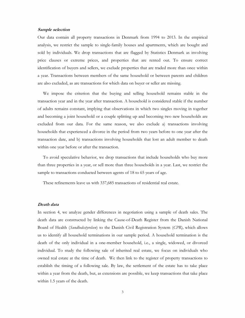
Our data contain all property transactions in Denmark from 1994 to 2013. In the empirical

analysis, we restrict the sample to single-family houses and apartments, which are bought and

sold by individuals. We drop transactions that are flagged by Statistics Denmark as involving

price clauses or extreme prices, and properties that are rented out. To ensure correct

identification of buyers and sellers, we exclude properties that are traded more than once within

a year. Transactions between members of the same household or between parents and children

are also excluded, as are transactions for which data on buyer or seller are missing.

We impose the criterion that the buying and selling household remains stable in the

transaction year and in the year after transaction. A household is considered stable if the number

of adults remains constant, implying that observations in which two singles moving in together

and becoming a joint household or a couple splitting up and becoming two new households are

excluded from our data. For the same reason, we also exclude a) transactions involving

households that experienced a divorce in the period from two years before to one year after the

transaction date, and b) transactions involving households that lost an adult member to death

within one year before or after the transaction.

To avoid speculative behavior, we drop transactions that include households who buy more

than three properties in a year, or sell more than three households in a year. Last, we restrict the

sample to transactions conducted between agents of 18 to 65 years of age.

These refinements leave us with 337,685 transactions of residential real estate.

Death data

In section 4, we analyze gender differences in negotiation using a sample of death sales. The

death data are constructed by linking the Cause-of-Death Register from the Danish National

Board of Health (Sundhedsstyrelsen) to the Danish Civil Registration System (CPR), which allows

us to identify all household terminations in our sample period. A household termination is the

death of the only individual in a one-member household, i.e., a single, widowed, or divorced

individual. To study the following sale of inherited real estate, we focus on individuals who

owned real estate at the time of death. We then link to the register of property transactions to

establish the timing of a following sale. By law, the settlement of the estate has to take place

within a year from the death, but, as extensions are possible, we keep transactions that take place

within 1.5 years of the death.

4

To identify the beneficiaries who are in charge of selling the property, we use the social

security number (CPR) to establish the link to all the children of the deceased. We restrict the

sample to household terminations with exactly one child, to ensure that we can identify the

decision maker in the selling process.

Copying the sample selection approach for the full sample, we combine data from several

registers to characterize the beneficiary (i.e., seller) in terms of family type, age, income, and

education. We also merge on the buyer information obtained in the full sample.

In addition, we apply all the selection criteria of the full sample to the death sales sample,

leaving us with 13,953 death sales.

Variable definition

The dependent variable is the log of the transaction price in thousand year-2015 DKK. The

hedonic model includes the following property characteristics: indicator for apartment, interior size

(in square meters), lot size (in square meters), number of rooms, number of bathrooms, age of the building

(in years), indicator for rural area, and municipality population size. All variables are from the BBR

register, except for the control for rural area, which is from a separate land register. In addition,

we introduce the log of the assessed value (measured in thousand year-2015 DKK) from the tax

authorities as additional control from Table 4 and onward.

We characterize the buyer and seller households using the unique household ID created by

Statistics Denmark. According to the definition used by Statistics Denmark, households consist

of one or two adults and the number of children living with them. We define three types of

households: couples, single women, and single men. Couples cover both married, registered, and

cohabiting partners, as defined by Statistics Denmark.

Household characteristics are from December 31 of the year previous to the trade year. Age is

average age of adult household members and is measured in years. Income is average income in

million year-2015 DKK, winsorized at the values of the 1 and 99 percentiles. College, Unemployed,

and Self-employed all take the values 0, 0.5, or 1, and indicate the share of adult household

members who have a college degree, are unemployed, or are self-employed, respectively. All

employment indicators are from November in the year before the transaction.

School-age children is an indicator for having children between 5 and 15 years old (the children

do not necessarily live in the household). Following the specification in HRS, we interact the

indicator for school-age children with the quarter of the transaction. First-time buyer indicates that

5

no one in the buyer household has previously owned real estate. Out-of-town buyer denotes that the

buyer lived in another municipality before buying.

6

Appendix B: A Model of Household Negotiation

This Appendix details the challenge of separating negotiation effects from demand effects and

discusses the solution suggested by Harding, Rosenthal, and Sirmans (2003) (henceforth HRS).

The market for heterogeneous goods, like the housing market, is often too thin to have a

clear market price. Instead, room exists for negotiation, leaving the price to be determined by the

negotiation between the buyer and the seller. HRS develop a model for identifying

characteristics-specific negotiation of agents.

The price of a heterogeneous good can be described by a hedonic price model (Rosen, 1974).

A good X is defined by a set of characteristics C, where X=X(C). The market price of X is the

product of C and a vector of shadow prices s(C):

P = s(C) * C .

(1)

For most heterogeneous goods, s is not directly observed, but as long as markets are

sufficiently thick, market participants can determine s, and s is still well-defined (Rosen, 1974).

However, as goods become more heterogeneous, the market becomes thinner. In the case of the

housing market, almost no houses are alike, making each transaction unique. When the

transaction is unique, s is not well-known. Because the requirements for perfect competition are

not met, excess surplus is not necessarily driven to zero. The buyer’s willingness to pay may be

larger than the seller’s willingness to accept, leaving excess surplus to be distributed between the

buyer and the seller. The trading partners will distribute this surplus through negotiating over the

price. HRS adds negotiation to the hedonic price model, now defining individual transaction i:

Pi = sCi + Bi .

(2)

sCi is the implicit market price of house i , which depends on the house characteristic. Bi is the

deviation from the market price, due to negotiation, which depends on the characteristics of the

buyer and the seller. If Bi is positive, the seller benefits from negotiation, and if Bi is negative, the

buyer benefits. That is, Bi reflects the relative bargaining power of the buyer and the seller, and

will be a function of buyer and seller characteristics. HRS remove the subscripts for simplicity

and express B as

B = bsell Dsell + bbuy Dbuy + eB ,

(3)

7

where D sell and D buy are vectors of the seller and buyer characteristics, respectively. b sell and b buy

are vectors of coefficients that describe the impact of seller and buyer characteristics on

negotiation. eB is idiosyncratic differences in negotiation. Substituting (3) into (2) gives

P = sC + bsell Dsell + bbuy Dbuy + eB ,

(4)

where b sell and b buy measure the effect of negotiation on the transaction price.

To use equation (4) to analyze gender differences in negotiation, we need to include all

relevant house characteristics in C and ensure that any unobserved characteristics are

uncorrelated with the characteristics of the buyer and seller. In practice, it is difficult to ensure

that the specification controls for all relevant characteristics. For instance, if women in general

buy houses with higher amenity values, and amenity values are unobserved in the data, the results

will imply that women pay more than men for the same house, when in fact they pay more due

to the amenity value. In that case, we would attribute the difference in amenity value to gender

differences in negotiation, rather than to differences in demand.

If C is fully observed by market participants but only partly observed by us, we need further

measures to ensure identification of negotiation. Harding, Rosenthal, and Sirmans (2003) assume

that C1 is observed by the researcher, but C2 is not. Different buyers and sellers may value C2

differently, which cause C2 to be correlated with D sell and D buy. The demand for the unobserved

characteristics of the house is

s2C2 = dsell Dsell + dbuy Dbuy + eD ,

(5)

where s2 is the vector of shadow prices on the unobserved characteristic, and eD is idiosyncratic

differences in preferences across individuals. Problematically, individual characteristics that affect

negotiation also influence demand for unobserved attributes of the house. If we substitute (5)

into (4) and rearrange, we cannot identify negotiation effects separately from demand effects:

P = s1C1 + ( bsell +dsell) Dsell +( bbuy +dbuy ) Dbuy + ε ,

(6)

where ε = eB + eD.

We need restrictions on bs and ds in order to identify negotiation. Harding, Rosenthal, and

Sirmans (2003) suggests two symmetry assumptions:

8

i) Symmetric bargaining power: bsell = – bbuy

ii) Symmetric demand: dsell = dbuy

Assumption i) implies that if buyers and sellers have identical characteristics, they will have

the same bargaining power, i.e., neither will have an advantage. Assumption ii) implies that if

buyers and sellers are identical, they value the houses equally, i.e., they have the same demand for

houses. These two symmetry assumptions cannot be tested.

Appling i) and ii) to (6) gives us

P = s1C1 + b (Dsell – Dbuyy) + d (Dsell + Dbuy) + ε ,

(7)

which is easily estimated by Ordinary Least Squares (OLS). If i) and ii) hold, then b will be a

measure of the effect of buyer and seller characteristics on bargaining power, independent of

differences in demand.

A positive b reflects a negotiation advantage, and a negative b reflects a negotiation

disadvantage. That is, if the coefficient to (womansell – womanbuy) is positive, the price is higher when

women are sellers or lower when women are buyers. Both reflect a good negotiation outcome

for women. If the coefficient to (womansell – womanbuy) is negative, then the price is lower when

women are sellers or higher when women are buyers. Both reflect a poor negotiation outcome

for women.

Importantly, we only have identification from transactions that involve different agents on

buyers’ and sellers’ sides, otherwise (Dsell – Dbuy) will be zero. In the case of gender, identification

comes from transactions involving different genders and not from transactions in which the

buyer and seller are the same gender.

Demand for unobserved characteristics of the house, like amenity value, appears in the

demand effect d, which captures differences in demand between different types of households.

We estimate negotiation, using pooled OLS and robust standard errors, by means of the

following equation:

Ln (priceit ) = β0 + s Ci + b (Disell – Di

buy) + d (Disell + Di

buy) + monthi + yeari +ui ,

(8)

where price is the transaction value, Ci is a vector of observed property characteristics, and Disell

and Dibuy are vectors of seller and buyer characteristics. monthi is a vector of month dummies, and

yeari is a vector of year dummies, both describing the timing of the transaction.

9

Because we take the log of the price, bwoman is the gender difference in negotiation, and a

positive coefficient indicates bargaining advantage of women measured in percent.

10

Appendix C: Adding wealth control

Table C1: Gender differences in negotiation (Table 3 with wealth control) This table shows gender differences in negotiation and demand using the estimation methodology of Harding, Rosenthal, and Sirmans (2003). The dependent variable is the log of transaction price in thousand year-2015 DKK. Data covers property transactions from 1994 to 2013, in which both the buyer and seller are stable households with a member between 18 and 65 years of age. Columns (1), (4), and (7) have the coefficients to the differences, i.e., the negotiation effects. Columns (2), (5), and (8) have the coefficients to the sums, i.e., the demand effects. Columns (1)–(3) contain only houses; (4)–(6), only apartments; and (7)–(9), both houses and apartments. Additional controls include: property characteristics, location indicators, quarter fixed effects, and year fixed effects. Robust standard errors are reported in parentheses. ***, **, and * indicate statistical significance at the 1%, 5%, and 10% levels, respectively.

Houses

Apartments

All Negotiation Demand Buyers only

Negotiation Demand Buyers only Negotiation Demand Buyers only

(1) (2) (3) (4) (5) (6) (7) (8) (9) Single female -0.020*** 0.090***

-0.002 0.073***

-0.020*** 0.089***

(0.003) (0.003)

(0.003) (0.003)

(0.003) (0.003) Single female x apartment

0.014*** -0.002

(0.005) (0.005) Couple -0.022*** 0.093***

-0.008*** 0.012***

-0.029*** 0.099***

(0.002) (0.002)

(0.003) (0.003)

(0.002) (0.002) Couple x apartment

0.043*** -0.067***

(0.004) (0.004) Age 0.002*** -0.003***

-0.000* -0.002***

0.002*** -0.003***

(0.000) (0.000)

(0.000) (0.000)

(0.000) (0.000) Income -0.055*** 0.253***

0.040*** 0.122***

-0.021*** 0.223***

(0.003) (0.002)

(0.003) (0.003)

(0.002) (0.002) Net wealth -0.006*** 0.021***

-0.004*** 0.007***

-0.004*** 0.019***

(0.001) (0.001)

(0.001) (0.001)

(0.000) (0.000) College -0.038*** 0.098***

-0.011*** 0.117***

-0.033*** 0.115***

(0.002) (0.002)

(0.002) (0.002)

(0.001) (0.001) Self-employed -0.015*** 0.045***

-0.011* 0.010*

-0.012*** 0.038***

(0.004) (0.004)

(0.006) (0.006)

(0.003) (0.003) School-age children x 1st quarter 0.003 -0.012***

0.020*** -0.044***

0.007*** -0.017***

(0.002) (0.002)

(0.005) (0.005)

(0.002) (0.002) School-age children x 2nd quarter 0.007*** -0.014***

0.021*** -0.034***

0.009*** -0.019***

(0.002) (0.002)

(0.005) (0.005)

(0.002) (0.002) School-age children x 3rd quarter 0.012*** -0.016***

0.025*** -0.040***

0.016*** -0.018***

(0.002) (0.002)

(0.005) (0.005)

(0.002) (0.002) School-age children x 4th quarter 0.004 -0.011***

0.030*** -0.051***

0.010*** -0.016***

(0.004) (0.004)

(0.009) (0.009)

(0.004) (0.003) First-time buyer

-0.032***

-0.007*

-0.028***

(0.002)

(0.004)

(0.002)

Out-of-town buyer

0.093***

0.082***

0.084***

(0.002)

(0.003)

(0.002)

Apartment

0.037***

(0.006)

Constant 6.390***

5.941***

6.289***

(0.008)

(0.014)

(0.008)

Additional controls: Property characteristics Yes

Yes

Yes

Location Yes

Yes

Yes Property fixed effects No

No

No

Quarter fixed effects Yes

Yes

Yes Year fixed effects Yes

Yes

Yes

Pseudo R2 0.630

0.680

0.614 Number of observations 269350 68335 337685

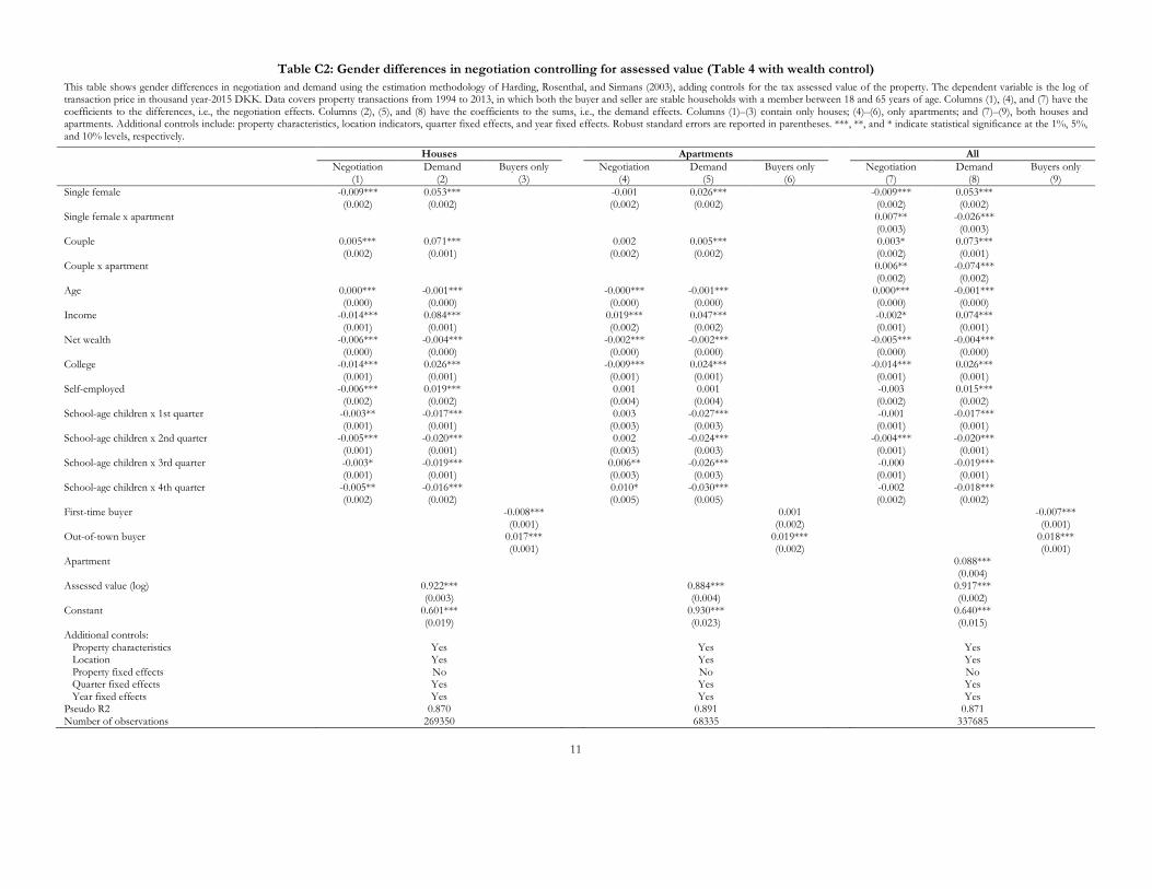
11

Table C2: Gender differences in negotiation controlling for assessed value (Table 4 with wealth control)

This table shows gender differences in negotiation and demand using the estimation methodology of Harding, Rosenthal, and Sirmans (2003), adding controls for the tax assessed value of the property. The dependent variable is the log of transaction price in thousand year-2015 DKK. Data covers property transactions from 1994 to 2013, in which both the buyer and seller are stable households with a member between 18 and 65 years of age. Columns (1), (4), and (7) have the coefficients to the differences, i.e., the negotiation effects. Columns (2), (5), and (8) have the coefficients to the sums, i.e., the demand effects. Columns (1)–(3) contain only houses; (4)–(6), only apartments; and (7)–(9), both houses and apartments. Additional controls include: property characteristics, location indicators, quarter fixed effects, and year fixed effects. Robust standard errors are reported in parentheses. ***, **, and * indicate statistical significance at the 1%, 5%, and 10% levels, respectively.

Houses

Apartments

All

Negotiation Demand Buyers only

Negotiation Demand Buyers only

Negotiation Demand Buyers only

(1) (2) (3)

(4) (5) (6)

(7) (8) (9) Single female -0.009*** 0.053***

-0.001 0.026***

-0.009*** 0.053***

(0.002) (0.002)

(0.002) (0.002)

(0.002) (0.002) Single female x apartment

0.007** -0.026***

(0.003) (0.003) Couple 0.005*** 0.071***

0.002 0.005***

0.003* 0.073***

(0.002) (0.001)

(0.002) (0.002)

(0.002) (0.001) Couple x apartment

0.006** -0.074***

(0.002) (0.002) Age 0.000*** -0.001***

-0.000*** -0.001***

0.000*** -0.001***

(0.000) (0.000)

(0.000) (0.000)

(0.000) (0.000) Income -0.014*** 0.084***

0.019*** 0.047***

-0.002* 0.074***

(0.001) (0.001)

(0.002) (0.002)

(0.001) (0.001) Net wealth -0.006*** -0.004***

-0.002*** -0.002***

-0.005*** -0.004***

(0.000) (0.000)

(0.000) (0.000)

(0.000) (0.000) College -0.014*** 0.026***

-0.009*** 0.024***

-0.014*** 0.026***

(0.001) (0.001)

(0.001) (0.001)

(0.001) (0.001) Self-employed -0.006*** 0.019***

0.001 0.001

-0.003 0.015***

(0.002) (0.002)

(0.004) (0.004)

(0.002) (0.002) School-age children x 1st quarter -0.003** -0.017***

0.003 -0.027***

-0.001 -0.017***

(0.001) (0.001)

(0.003) (0.003)

(0.001) (0.001) School-age children x 2nd quarter -0.005*** -0.020***

0.002 -0.024***

-0.004*** -0.020***

(0.001) (0.001)

(0.003) (0.003)

(0.001) (0.001) School-age children x 3rd quarter -0.003* -0.019***

0.006** -0.026***

-0.000 -0.019***

(0.001) (0.001)

(0.003) (0.003)

(0.001) (0.001) School-age children x 4th quarter -0.005** -0.016***

0.010* -0.030***

-0.002 -0.018***

(0.002) (0.002)

(0.005) (0.005)

(0.002) (0.002) First-time buyer

-0.008***

0.001

-0.007***

(0.001)

(0.002)

(0.001)

Out-of-town buyer

0.017***

0.019***

0.018***

(0.001)

(0.002)

(0.001)

Apartment

0.088***

(0.004)

Assessed value (log) 0.922***

0.884***

0.917***

(0.003)

(0.004)

(0.002)

Constant 0.601***

0.930***

0.640***

(0.019)

(0.023)

(0.015)

Additional controls: Property characteristics Yes

Yes

Yes

Location Yes

Yes

Yes Property fixed effects No

No

No

Quarter fixed effects Yes

Yes

Yes Year fixed effects Yes

Yes

Yes

Pseudo R2 0.870

0.891

0.871 Number of observations 269350 68335 337685

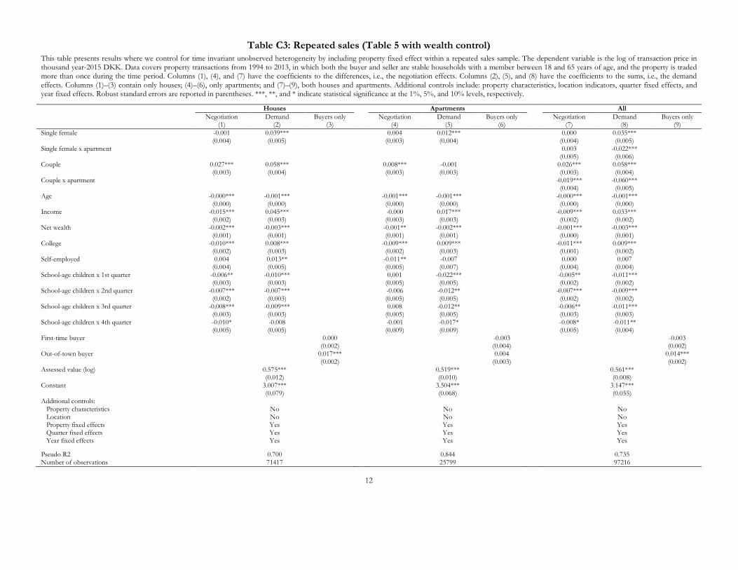
12

Table C3: Repeated sales (Table 5 with wealth control) This table presents results where we control for time invariant unobserved heterogeneity by including property fixed effect within a repeated sales sample. The dependent variable is the log of transaction price in thousand year-2015 DKK. Data covers property transactions from 1994 to 2013, in which both the buyer and seller are stable households with a member between 18 and 65 years of age, and the property is traded more than once during the time period. Columns (1), (4), and (7) have the coefficients to the differences, i.e., the negotiation effects. Columns (2), (5), and (8) have the coefficients to the sums, i.e., the demand effects. Columns (1)–(3) contain only houses; (4)–(6), only apartments; and (7)–(9), both houses and apartments. Additional controls include: property characteristics, location indicators, quarter fixed effects, and year fixed effects. Robust standard errors are reported in parentheses. ***, **, and * indicate statistical significance at the 1%, 5%, and 10% levels, respectively.

Houses

Apartments

All

Negotiation Demand Buyers only

Negotiation Demand Buyers only

Negotiation Demand Buyers only

(1) (2) (3)

(4) (5) (6)

(7) (8) (9) Single female -0.001 0.039***

0.004 0.012***

0.000 0.035***

(0.004) (0.005)

(0.003) (0.004)

(0.004) (0.005) Single female x apartment

0.003 -0.022***

(0.005) (0.006) Couple 0.027*** 0.058***

0.008*** -0.001

0.026*** 0.058***

(0.003) (0.004)

(0.003) (0.003)

(0.003) (0.004) Couple x apartment

-0.019*** -0.060***

(0.004) (0.005) Age -0.000*** -0.001***

-0.001*** -0.001***

-0.000*** -0.001***

(0.000) (0.000)

(0.000) (0.000)

(0.000) (0.000) Income -0.015*** 0.045***

-0.000 0.017***

-0.009*** 0.033***

(0.002) (0.003)

(0.003) (0.003)

(0.002) (0.002) Net wealth -0.002*** -0.003***

-0.001** -0.002***

-0.001*** -0.003***

(0.001) (0.001)

(0.001) (0.001)

(0.000) (0.001) College -0.010*** 0.008***

-0.009*** 0.009***

-0.011*** 0.009***

(0.002) (0.003)

(0.002) (0.003)

(0.001) (0.002) Self-employed 0.004 0.013**

-0.011** -0.007

0.000 0.007

(0.004) (0.005)

(0.005) (0.007)

(0.004) (0.004) School-age children x 1st quarter -0.006** -0.010***

0.001 -0.022***

-0.005** -0.011***

(0.003) (0.003)

(0.005) (0.005)

(0.002) (0.002) School-age children x 2nd quarter -0.007*** -0.007***

-0.006 -0.012**

-0.007*** -0.009***

(0.002) (0.003)

(0.005) (0.005)

(0.002) (0.002) School-age children x 3rd quarter -0.008*** -0.009***

0.008 -0.012**

-0.006** -0.011***

(0.003) (0.003)

(0.005) (0.005)

(0.003) (0.003) School-age children x 4th quarter -0.010* -0.008

-0.001 -0.017*

-0.008* -0.011**

(0.005) (0.005)

(0.009) (0.009)

(0.005) (0.004) First-time buyer

0.000

-0.003

-0.003

(0.002)

(0.004)

(0.002)

Out-of-town buyer

0.017***

0.004

0.014***

(0.002)

(0.003)

(0.002)

Assessed value (log) 0.575***

0.519***

0.561***

(0.012)

(0.010)

(0.008)

Constant 3.007***

3.504***

3.147***

(0.079)

(0.068)

(0.055)

Additional controls: Property characteristics No

No

No

Location No

No

No Property fixed effects Yes

Yes

Yes

Quarter fixed effects Yes

Yes

Yes Year fixed effects Yes

Yes

Yes

Pseudo R2 0.700

0.844

0.735 Number of observations 71417 25799 97216

13

Table C4: Gender differences when selling inherited properties (Table 7 with wealth control) This table applies the negotiation model of Harding, Rosenthal, and Sirmans (2003) on our sample of inherited properties. We modify the model such that differences between seller (the beneficiary) and buyer characteristics capture negotiation effects and sums of owner (the deceased) and buyer characteristics capture demand effects. The dependent variable is the log of transaction price in thousands year-2015 DKK. Data covers estate sales due to deaths from 1994 to 2013. Columns (1), (3), and (5) have the coefficients to the differences, i.e., the negotiation effects. Columns (2), (4), and (6) have the coefficients to the sums, i.e., the demand effects. Columns (1)–(2) contain only houses; (3)–4), only apartments; and (5)–(6), both houses and apartments. Additional controls include: quarter fixed-effects, and year fixed-effects. Robust standard errors are reported in parentheses. ***, **, and * indicate statistical significance at the 1%, 5%, and 10% levels, respectively.

Houses Apartments All

Negotiation Demand

Negotiation Demand

Negotiation Demand

(1) (2) (3) (4) (5) (6)

Single female -0.005 0.019***

0.021 0.042***

-0.004 0.019***

(0.008) (0.005)

(0.017) (0.013)

(0.008) (0.005)

Single female x apartment

0.023 0.022

(0.020) (0.014)

Couple 0.024*** 0.070***

0.011 0.030

0.023*** 0.072***

(0.007) (0.007)

(0.019) (0.023)

(0.007) (0.007)

Couple x apartment

-0.009 -0.036

(0.019) (0.023)

Age 0.003*** 0.001***

0.002*** 0.001**

0.002*** 0.001***

(0.000) (0.000)

(0.001) (0.000)

(0.000) (0.000)

Income -0.014* 0.010***

0.001 -0.002

-0.013* 0.009***

(0.007) (0.003)

(0.014) (0.007)

(0.007) (0.003)

Net wealth 0.005*** -0.001**

-0.000 0.001*

0.004*** -0.000

(0.002) (0.000)

(0.003) (0.001)

(0.001) (0.000)

College 0.015** 0.023***

-0.008 0.046***

0.011** 0.026***

(0.006) (0.007)

(0.014) (0.016)

(0.005) (0.006)

Self-employed 0.065* -0.005

0.077 0.215***

0.071** 0.029

(0.036) (0.040)

(0.069) (0.072)

(0.033) (0.038)

Children (dummy) 0.015*** 0.001

0.030** 0.016

0.017*** 0.003

(0.006) (0.008)

(0.015) (0.021)

(0.006) (0.008)

Apartment

0.085***

(0.023)

Constant -0.464***

0.391**

-0.395***

(0.055)

(0.171)

(0.053)

Additional controls: Property characteristics No

No

No

Location No

No

No Property fixed effects No

No

No

Quarter fixed effects Yes

Yes

Yes Year fixed effects Yes

Yes

Yes

Pseudo R2 0.832

0.836

0.830

Number of observations 12633 1320 13953

14

Appendix D: Extra descriptive statistics

Table D1: Buyer and seller characteristics (repeated sales)

This table shows characteristics of buyers and sellers in 97,216 property transactions from 1994 to 2013, in which both buyers and sellers are between 18 and 65 years of age and did not experience a change in the composition of adult household members around the time of trade. Also, the property has been traded more than once during the period. Households consist of one or two adults living together and the number of children living with them. A household takes part in a transaction if at least one adult in the household buys or sells property. Buyers are identified as the owners of the property the year after the transaction, while sellers are identified as the owners of the property, registered the January 1, in the year of the transaction. We take household characteristics from December 31 in the year before the transaction year. Age is mean age of the adult household members. Income and net wealth are household totals in 2015-prices, winsorized at 1 percent in both ends, and presented in millions Danish kroner. College is the share of adult household members with a college degree. Self-employed is the share of adult household members that are self-employed. All shares take values 0, 0.5, or 1. School-age children is a dummy for having children between 5 and 15 years old (the children do not necessarily live in the household). First-time buyer indicates that no member of the household has previously owned real estate. Standard deviations are presented in parentheses for non-indicator variables. t-statistics are in brackets. *** indicates significance at the 1% level.

Buyers Sellers

All

Single women

Single men Difference All

Single women

Single men Difference

Age 38.23 39.75 35.14 4.62*** 41.57 46.54 40.83 5.71***

(11.38) (12.12) (11.25) [27.8] (11.5) (12.24) (11.88) [32.81]

Income (100,000 DKR) 3.68 3.44 3.61 -0.17*** 3.74 3.41 3.81 -0.41***

(2.04) (1.95) (2.12) [-5.86] (1.88) (1.78) (2.17) [-14.02]

Net wealth (mil. DKR) 0.44 0.44 0.27 0.16*** 0.48 0.62 0.40 0.22***

(1.49) (1.2) (1.09) [10.16] (1.46) (1.31) (1.26) [12.09]

College 0.27 0.34 0.20 0.14*** 0.26 0.30 0.19 0.11***

[22.1]

[17.61]

Self-employed 0.04 0.03 0.03 0.00 0.04 0.03 0.04 -0.01***

[-1.48]

[-5.08]

School-age children 0.26 0.16 0.13 0.03*** 0.32 0.15 0.18 -0.03***

[5.78]

[-6.51]

First-time buyer 0.31 0.43 0.52 -0.10***

[-13.84]

Out-of-town buyer 0.48 0.41 0.41 -0.01

[-0.83]

N 97,216 8,806 11,119

97,216 9,082 10,107

15

Table D2: Property characteristics (repeated sales)

This table shows characteristics of properties traded more than once during 1994-2013, separately for houses and apartments. Price is the realized sales price, and assessed value is the assessed value of the property from the Danish tax authorities prior to the sales. Both prices and assessed value are measured in thousand year-2015 DKK. Interior size and Lot size are measured in square meters. House age and building age are measured in years. Rooms and bathrooms are count variables. Rural indicates a rural area. Standard deviations are presented in parentheses for non-indicator variables. t-statistics are in brackets. *** and ** indicate significance at the 1% and 5% levels, respectively.

Buyers Sellers

All Single

women (1)

Single men (2)

Difference (1)–(2)

Single

women (1)

Single men (2)

Difference (1)–(2)

A. Houses Number of transactions 71,417 4,371 5,122 5,608 5,933 Price (1000 DKK) 1431.15 1185.69 1009.47 176.21*** 1238.89 1117.85 121.04***

(1007.31) (928.7) (815.5) [9.84] (1084.52) (914.67) [6.49]

Assessed value 1141.18 963.59 850.95 112.64*** 1034.27 951.78 82.49***

(768.38) (695.9) (632.44) [8.26] (797.57) (726.21) [5.81]

Interior size (m2) 114.46 96.84 95.22 1.62** 107.10 104.65 2.45***

(44.53)

(35.4) (35.8) [2.21] (43.98) (43.93) [3]

Lot size (m2) 983.41 774.47 901.78 -127.31*** 969.81 1010.33 -40.52

(1260.81) (1545.47) (817.29) [-5.12] (1937.85) (1144.19) [-1.38]

House age (years) 43.36 52.01 52.64 -0.63 49.36 49.73 -0.38

(33.75) (39.52) (39.55) [-0.78] (36.65) (38) [-0.54] Rooms (#) 4.28 3.75 3.71 0.04* 4.07 3.99 0.07***

(1.26) (1.07) (1.14) [1.76] (1.27) (1.27) [3.15] Bathrooms (#) 1.34 1.17 1.14 0.03*** 1.27 1.23 0.04***

(0.54) (0.44) (0.41) [3.82] (0.52) (0.5) [3.71] Rural 0.34 0.33 0.42 -0.10*** 0.37 0.42 -0.05***

[-9.58] [-5.45]

B. Apartments Number of transactions 25,799 4,435 5,997 3,474 4,174 Price (1000 DKK) 1288.11 1166.02 1065.03 100.98*** 1164.61 1078.96 85.65***

(817.16) (705.53) (659.09) [7.51] (703.48) (668.7) [5.45]

Assessed value 1040.41 939.38 861.35 78.03*** 942.75 866.01 76.74***

(688.6) (625.65) (539.89) [6.82] (611.08) (555.22) [5.75]

Interior size (m2) 74.59

70.19 67.91 2.28*** 68.78 66.38 2.40***

(27.42)

(23.06) (21.98) [5.13] (24.36) (24.34) [4.29]

Building age (years) 66.37

65.33 64.27 1.06 66.58 65.50 1.08

(35.67)

(35.48) (34.95) [1.52] (35.89) (35.92) [1.31] Rooms (#) 2.63

2.46 2.36 0.11*** 2.41 2.30 0.11***

(1.03)

(0.88) (0.87) [6.3] (0.94) (0.93) [5.01]

Bathrooms (#) 1.03

1.02 1.01 0.01** 1.02 1.01 0.01

(0.22)

(0.17) (0.15) [2.28] (0.18) (0.18) [1.45] Rural 0.01

0.00 0.01 0.00** 0.01 0.01 0.00

[-1.97] [-0.62]

16

Table D3: Identifying differences in seller and buyer characteristics

This table shows the frequencies for seller-buyer differences in indicator variables in the samples. Single female indicates a household consisting of one adult female. Apartment indicates that the traded property is an apartment. College is the share of adult household members with a college degree. Self-employed is the share of adult household members that are self-employed. School-age children is a dummy for having children between 5 and 15 years old. Percentages are presented in parentheses.

Full Sample Repeat Sample

Seller – buyer -1 -0.5 0 0.5 1 -1 -0.5 0 0.5 1

Single female 24,607 - 282,184 - 30,894 7,513 - 81,914 - 7,789

(7.3) (83.6) (9.1) (7.7) (84.3) (8)

Apartment * single female 10,351 - 319,823 - 7,511 3,681 - 90,815 - 2,720

(3.1) (94.7) (2.2) (3.8) (93.4) (2.8)

Couple 51,629 - 240,895 - 45,161 13,167 - 70,146 - 13,903

(15.3) (71.3) (13.4) (13.5) (72.2) (14.3)

Apartment * couple 10,867 - 307,693 - 19,125 4,028 - 86,376 - 6,812

(3.2) (91.1) (5.7) (4.1) (88.8) (7)

College 33,551 51,421 182,317 44,614 25,782 9,234 14,077 51,942 13,651 8,312

(9.9) (15.2) (54) (13.2) (7.6) (9.5) (14.5) (53.4) (14) (8.6)

Self-employed 2,415 16,646 296,811 18,797 3,016 731 5,028 84,999 5,551 907

(0.7) (4.9) (87.9) (5.6) (0.9) (0.8) (5.2) (87.4) (5.7) (0.9)

School-age children 62,988 - 205,734 - 68,963 15,765 - 60,127 - 21,324

(18.7) (60.9) (20.4) (16.2) (61.8) (21.9)

N 337,685 97,216

17

Table D4: Buyer and seller combinations

The table shows the frequencies of all buyer-seller combinations. Panel A has buyer-seller combinations for the full sample used in Table 1 to Table 4. Panel B has buyer-seller combinations for the repeat sales sample in Table 5.

(A) Full Sample

Seller\buyer Couple Single male Single female Total

Couple 221,104 24,704 20,457 266,265

Single male 25,803 6,460 4,150 36,413

Single female 25,826 5,068 4,113 35,007

Total 272,733 36,232 28,720 337,685

(B) Repeat sales samples

Seller\buyer Couple Single male Single female Total

Couple 64,124 7,662 6,241 78,027

Single male 6,872 1,963 1,272 10,107

Single female 6,295 1,494 1,293 9,082

Total 77,291 11,119 8,806 97,216

18

Appendix E: Hedonic model without demand effects Table E1: Hedonic model without demand effects

This table shows gender differences in sales prices by buyer and seller characteristics using a simple hedonic regression. The dependent variable is the log of transaction price in thousand year-2015 DKK. Data covers property transactions from 1994 to 2013, in which both the buyer and seller are stable households with a member between 18 and 65 years of age. Columns (1–3), (6–8), and (11–13) have all sales, while columns (4–5), (9–10), and (15–15) only look at properties that are traded twice within the period (resales). Columns (1)–(5) contain only houses; (6)–(10), only apartments; and (11)–(15), both houses and apartments. Additional controls include those for: gender and role (controls for couples buying and selling, as well as interactions of these), property characteristics, location indicators, quarter fixed effects, and year fixed effects. Only coefficients on the variable of interest, female buyers and female sellers, are reported. Robust standard errors are reported in parentheses. ***, **, and * indicate statistical significance at the 1%, 5%, and 10% levels, respectively. The linear test of whether female buyers and sellers trade at the same price is reported in the bottom of the table as p-values of the test.

Houses

Apartments

All

Specification

Baseline +

Tax Value Baseline

+ Property

Fixed

Effects Baseline +

Tax Value Baseline

+ Fixed

Effects Baseline +

Tax Value Baseline

+ Fixed

Effects

(1) (2) (3) (4) (5) (6) (7) (8) (9) (10) (11) (12) Sample Full Full Resales Resales Full Full Resales Resales Full Full Resales Resales

Single female buyer 0.098*** 0.048*** 0.035** 0.000 0.073*** 0.039*** 0.039*** 0.022** 0.097*** 0.048*** 0.037** -0.018

(0.013) (0.009) (0.017) (0.020) (0.009) (0.006) (0.009) (0.011) (0.013) (0.009) (0.017) (0.019)

Single female seller 0.058*** 0.026*** 0.009 -0.013 0.064*** 0.028*** 0.030*** 0.023** 0.056*** 0.026*** 0.011 -0.030

(0.013) (0.009) (0.017) (0.020) (0.008) (0.006) (0.009) (0.010) (0.013) (0.009) (0.018) (0.020)

Single Female buyer x Apartment -0.018 -0.008 0.004 0.050**

(0.016) (0.011) (0.020) (0.022)

Single Female seller x Apartment 0.002 -0.002 0.015 0.061***

(0.016) (0.011) (0.020) (0.022)

Additional controls:

Interaction of Gender and Role Yes Yes Yes Yes Yes Yes Yes Yes Yes Yes Yes Yes

Individual Buyer and Seller

Characteristics

Yes Yes Yes Yes Yes Yes Yes Yes Yes Yes Yes Yes

Tax evaluations No Yes Yes Yes No Yes Yes Yes No Yes Yes Yes

Property characteristics Yes Yes Yes Yes Yes Yes Yes Yes Yes Yes Yes Yes

Location Yes Yes Yes Yes Yes Yes Yes Yes Yes Yes Yes Yes

Property fixed effects No No No Yes No No No Yes No No No Yes

Quarter fixed effects Yes Yes Yes Yes Yes Yes Yes Yes Yes Yes Yes Yes

Year fixed effects Yes Yes Yes Yes Yes Yes Yes Yes Yes Yes Yes Yes

Pseudo R2 0.663 0.871 0.875 0.700 0.751 0.894 0.898 0.844 0.661 0.873 0.877 0.736

N 269,350 269,350 71,417 71,417 68,335 68,335 25,799 25,799 337,685 337,685 97,216 97,216

P-values for test of Single female seller =

Single female buyer

0.002 0.017 0.172 0.505 0.364 0.076 0.327 0.933 0.002 0.018 0.177 0.564

P-values for test of Single female seller x Apartment =Single female buyer x Apartment

0.227 0.593 0.625 0.650

19

Appendix F: Robustness analyses Table F1: Gender differences in negotiation controlling for assessed value and ownership length

This table shows gender differences in negotiation and demand using the estimation methodology of Harding, Rosenthal, and Sirmans (2003), adding controls for the tax assessed value of the property and the ownership length, measured in years from acquisition date to sales date. The dependent variable is the log of transaction price in thousand year-2015 DKK. Data covers property transactions from 1994 to 2013, in which both the buyer and seller are stable households with a member between 18 and 65 years of age. Columns (1), (4), and (7) have the coefficients to the differences, i.e., the negotiation effects. Columns (2), (5), and (8) have the coefficients to the sums, i.e., the demand effects. Columns (1)–(3) contain only houses; (4)–(6), only apartments; and (7)–(9), both houses and apartments. Additional controls include: buyer and seller characteristics, property characteristics, location indicators, quarter fixed effects, and year fixed effects. Robust standard errors are reported in parentheses. ***, **, and * indicate statistical significance at the 1%, 5%, and 10% levels, respectively.

Houses Apartments All

Bargaining Demand Other controls

Bargaining Demand Other controls

Bargaining Demand Other controls

(1) (2) (3) (4) (5) (6) (7) (8) (9) Single female -0.011*** 0.052***

-0.005** 0.022***

-0.012*** 0.051***

(0.002) (0.002)

(0.002) (0.002)

(0.002) (0.002) Single female x apartment

0.005* -0.028***

(0.003) (0.003) Couple 0.006*** 0.073***

-0.001 0.003*

0.003** 0.075***

(0.002) (0.002)

(0.002) (0.002)

(0.002) (0.002) Couple x apartment

0.001 -0.078***

(0.002) (0.002) Ownership length

-0.003***

-0.007***

-0.004***

(0.000)

(0.000)

(0.000)

Ownership length x apartment

-0.003***

(0.001)

Ownership length x female seller

0.002***

0.004***

0.002***

(0.000)

(0.001)

(0.000)

Ownership length x female seller x apartment

0.002***

(0.001)

Ownership length x couple seller

0.002***

0.002***

0.002***

(0.000)

(0.000)

(0.000)

Ownership length x couple seller x apartment

0.001*

(0.001)

Apartment 0.099***

(0.004)

Assessed value (log) 0.917*** 0.882*** 0.913***

(0.003) (0.004) (0.002)

Constant 0.632*** 0.933*** 0.662***

(0.003) (0.005) (0.002) Additional controls:

Buyer and seller characteristics Yes

Yes

Yes Property characteristics Yes

Yes

Yes

Location Yes

Yes

Yes Property fixed effects No

No

No

Quarter fixed effects Yes

Yes

Yes Year fixed effects Yes

Yes

Yes

Pseudo R2 0.869

0.892

0.871 Number of observations 269350 68335 337685

20

Table F2: Repeated sales, no property fixed effects This table presents results where we control for time invariant unobserved heterogeneity by including property fixed effect within a repeated sales sample. The dependent variable is the log of transaction price in thousand year-2015 DKK. NOTE: we do not apply property fixed effects here. Data covers property transactions from 1994 to 2013, in which both the buyer and seller are stable households with a member between 18 and 65 years of age, and the property is traded more than once during the time period. Columns (1), (4), and (7) have the coefficients to the differences, i.e., the negotiation effects. Columns (2), (5), and (8) have the coefficients to the sums, i.e., the demand effects. Columns (1)–(3) contains only houses; (4)–(6), only apartments; and (7)–(9), both houses and apartments. Additional controls include: property characteristics, location indicators, quarter fixed effects, and year fixed effects. Robust standard errors are reported in parentheses. ***, **, and * indicate statistical significance at the 1%, 5%, and 10% levels.

Houses Apartments All

Bargaining Demand Other controls

Bargaining Demand Other controls

Bargaining Demand Other controls

(1) (2) (3) (4) (5) (6) (7) (8) (9) Single female -0.008** 0.050***

-0.001 0.022***

-0.008** 0.050***

(0.004) (0.004)

(0.003) (0.003)

(0.004) (0.004) Single female x apartment

0.004 -0.028***

(0.005) (0.005) Couple 0.015*** 0.069***

0.001 0.004

0.012*** 0.071***

(0.003) (0.003)

(0.003) (0.003)

(0.003) (0.003) Couple x apartment

-0.008* -0.072***

(0.004) (0.004) Age 0.000 -0.001***

-0.000*** -0.001***

0.000 -0.001***

(0.000) (0.000)

(0.000) (0.000)

(0.000) (0.000) Income -0.017*** 0.076***

0.012*** 0.039***

-0.003 0.063***

(0.002) (0.002)

(0.003) (0.003)

(0.002) (0.002) College -0.011*** 0.022***

-0.008*** 0.025***

-0.012*** 0.023***

(0.002) (0.002)

(0.002) (0.002)

(0.001) (0.001) Self-employed -0.005 0.018***

-0.008 -0.012**

-0.005 0.009**

(0.004) (0.004)

(0.006) (0.006)

(0.003) (0.003) School-age children x 1st quarter -0.002 -0.016***

0.005 -0.029***

-0.001 -0.016***

(0.002) (0.002)

(0.005) (0.005)

(0.002) (0.002) School-age children x 2nd quarter -0.005** -0.017***

0.001 -0.020***

-0.004* -0.018***

(0.002) (0.002)

(0.004) (0.004)

(0.002) (0.002) School-age children x 3rd quarter -0.001 -0.021***

0.009* -0.025***

0.001 -0.021***

(0.003) (0.003)

(0.005) (0.005)

(0.002) (0.002) School-age children x 4th quarter -0.004 -0.010**

0.010 -0.028***

-0.001 -0.014***

(0.005) (0.004)

(0.009) (0.008)

(0.004) (0.004) First-time buyer

-0.010***

-0.003

-0.009***

(0.002)

(0.003)

(0.002)

Out-of-town buyer

0.018***

0.015***

0.018***

(0.002)

(0.003)

(0.002)

Apartment 0.087*** (0.007) Assessed value (log) 0.908*** 0.874*** 0.904*** (0.004) (0.006) (0.003) Constant 0.706*** 1.014*** 0.750*** (0.028) (0.035) (0.021) Additional controls:

Property characteristics Yes

Yes

Yes Location Yes

Yes

Yes

Property fixed effects No

No

No Quarter fixed effects Yes

Yes

Yes

Year fixed effects Yes

Yes

Yes Pseudo R2 0.873

0.895

0.875

Number of observations 71417 25799 97216