gene expression and the transcriptome i. genomics and transcriptome after genome sequencing and...
Post on 22-Dec-2015
224 views
TRANSCRIPT
Gene expression and the transcriptome I
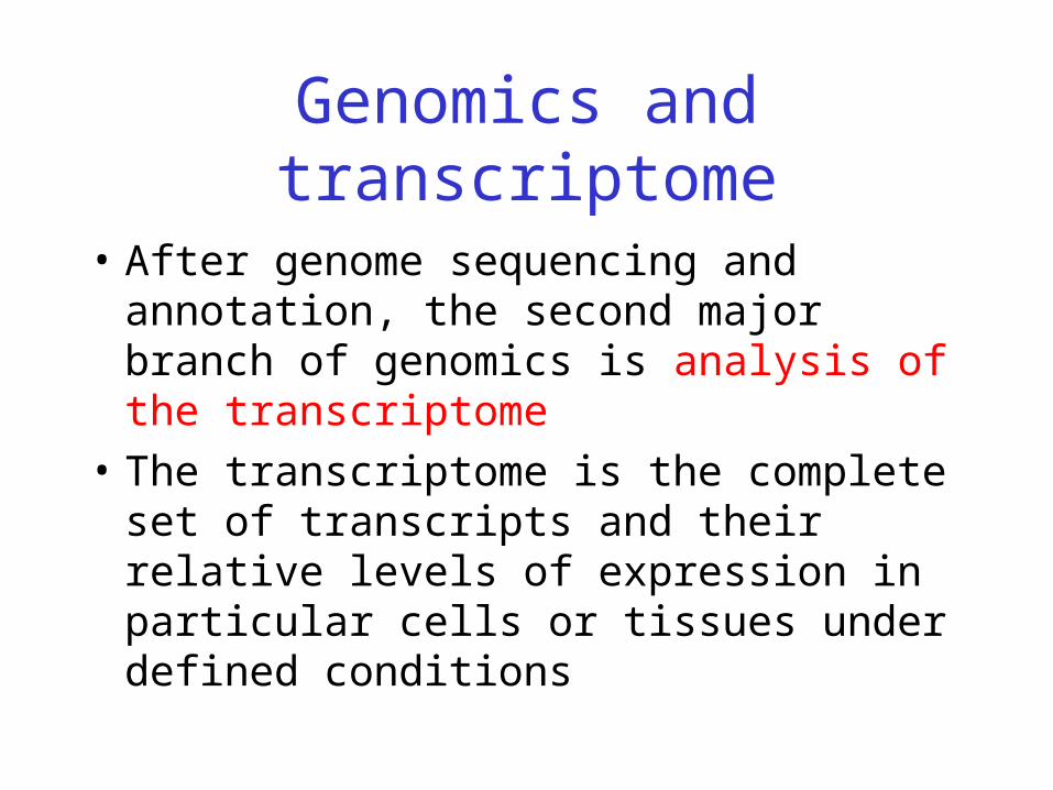
Genomics and transcriptome
• After genome sequencing and annotation, the second major branch of genomics is analysis of the transcriptome
• The transcriptome is the complete set of transcripts and their relative levels of expression in particular cells or tissues under defined conditions
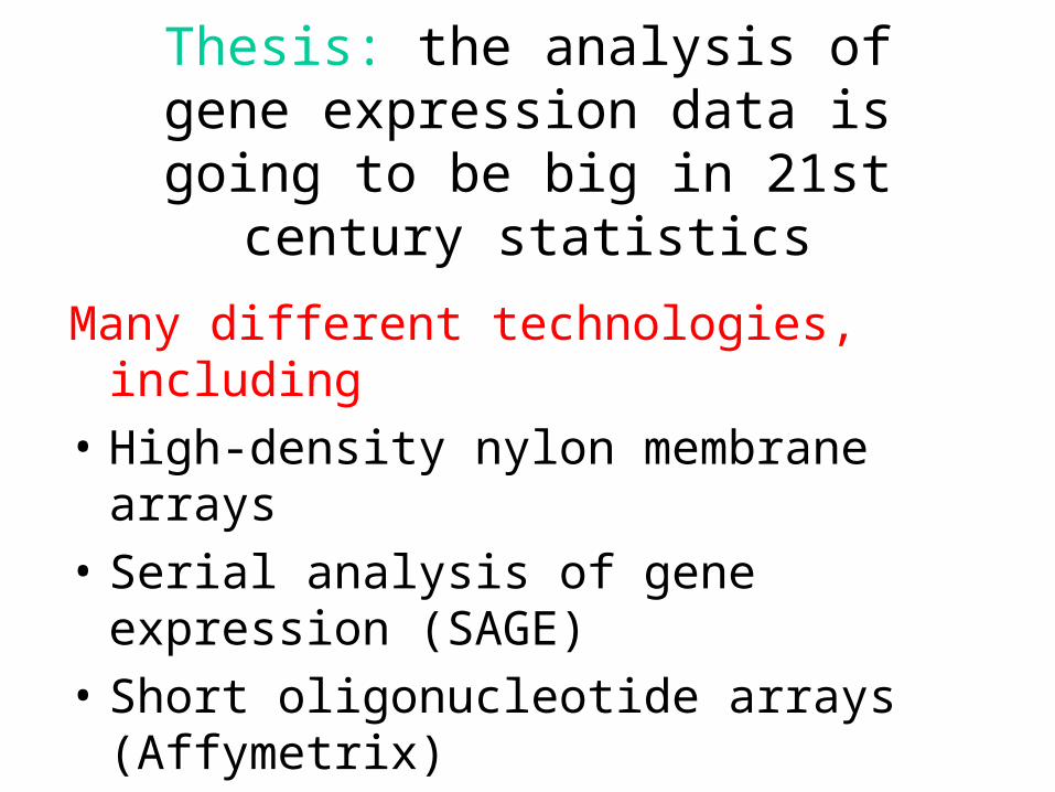
Thesis: the analysis of gene expression data is going to be big in 21st century
statistics
Many different technologies, including
• High-density nylon membrane arrays
• Serial analysis of gene expression (SAGE)
• Short oligonucleotide arrays (Affymetrix)
• Long oligo arrays (Agilent)
• Fibre optic arrays (Illumina)
• cDNA arrays (Brown/Botstein)*
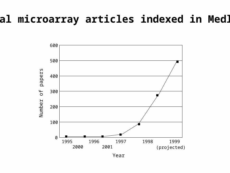
1995 1996 1997 1998 1999 2000 2001
0
100
200
300
400
500
600
(projected)
Year
Num
ber
of
papers
Total microarray articles indexed in Medline
Common themes
• Parallel approach to collection of very large amounts of data (by biological standards)
• Sophisticated instrumentation, requires some understanding
• Systematic features of the data are at least as important as the random ones
• Often more like industrial process than single investigator lab research
• Integration of many data types: clinical, genetic, molecular…..databases
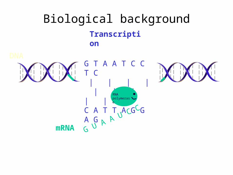
Biological background
G T A A T C C T C | | | | | | | | | C A T T A G G A G
DNA
G U A A U C C
RNA polymerase
mRNA
Transcription
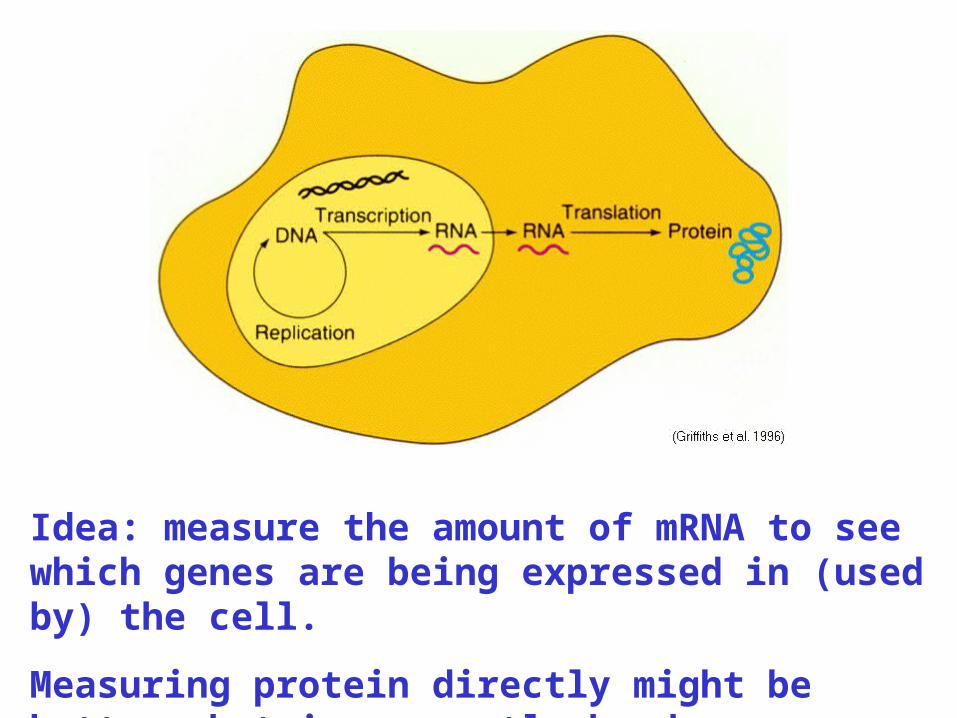
Idea: measure the amount of mRNA to see which genes are being expressed in (used by) the cell.
Measuring protein directly might be better, but is currently harder.
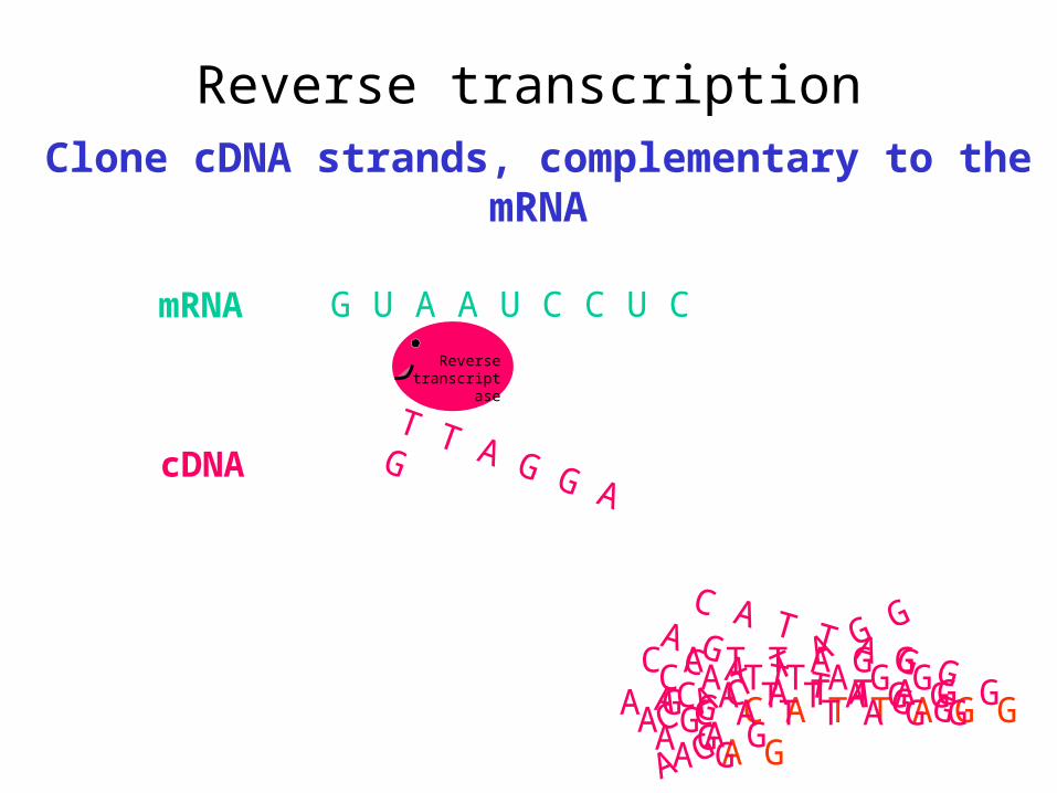
Reverse transcriptionClone cDNA strands, complementary to the mRNA
G U A A U C C U C
Reverse transcriptase
mRNA
cDNA
C A T T A G G A G C A T T A G G A G C A T T A G G A G C A T T A G G A G
T T A G G A G
C A T T A G G A G C A T T A G G A G C A T T A G G A G
C A T T A G G A G
C A T T A G G A G
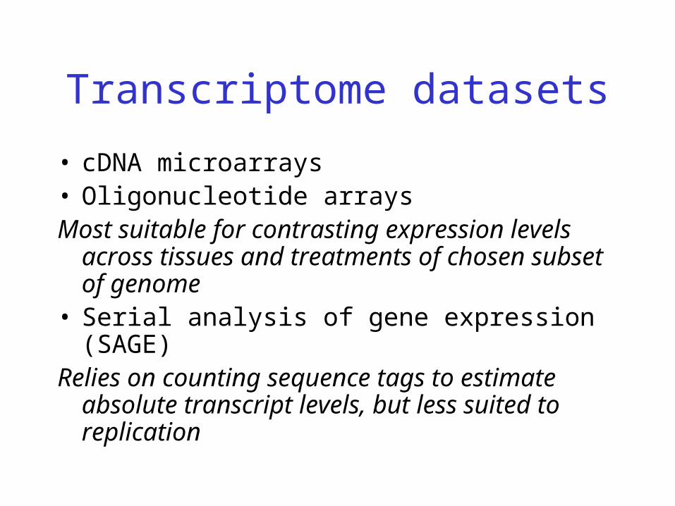
Transcriptome datasets
• cDNA microarrays • Oligonucleotide arraysMost suitable for contrasting expression levels
across tissues and treatments of chosen subset of genome
• Serial analysis of gene expression (SAGE)Relies on counting sequence tags to estimate
absolute transcript levels, but less suited to replication
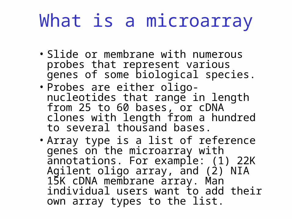
What is a microarray
• Slide or membrane with numerous probes that represent various genes of some biological species.
• Probes are either oligo-nucleotides that range in length from 25 to 60 bases, or cDNA clones with length from a hundred to several thousand bases.
• Array type is a list of reference genes on the microarray with annotations. For example: (1) 22K Agilent oligo array, and (2) NIA 15K cDNA membrane array. Man individual users want to add their own array types to the list.
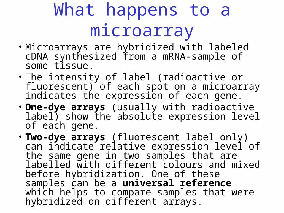
What happens to a microarray
• Microarrays are hybridized with labeled cDNA synthesized from a mRNA-sample of some tissue.
• The intensity of label (radioactive or fluorescent) of each spot on a microarray indicates the expression of each gene.
• One-dye arrays (usually with radioactive label) show the absolute expression level of each gene.
• Two-dye arrays (fluorescent label only) can indicate relative expression level of the same gene in two samples that are labelled with different colours and mixed before hybridization. One of these samples can be a universal reference which helps to compare samples that were hybridized on different arrays.
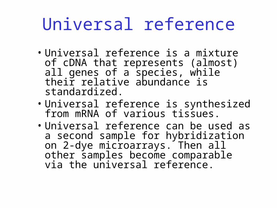
Universal reference
• Universal reference is a mixture of cDNA that represents (almost) all genes of a species, while their relative abundance is standardized.
• Universal reference is synthesized from mRNA of various tissues.
• Universal reference can be used as a second sample for hybridization on 2-dye microarrays. Then all other samples become comparable via the universal reference.
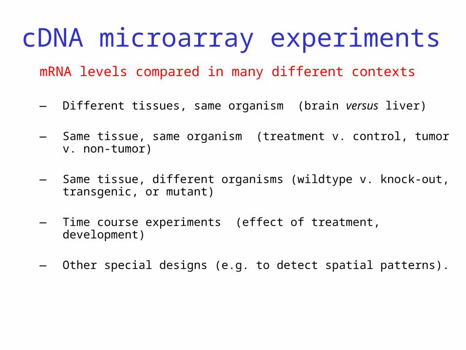
cDNA microarray experimentsmRNA levels compared in many different contexts
— Different tissues, same organism (brain versus liver)
— Same tissue, same organism (treatment v. control, tumor v. non-tumor)
— Same tissue, different organisms (wildtype v. knock-out, transgenic, or mutant)
— Time course experiments (effect of treatment, development)
— Other special designs (e.g. to detect spatial patterns).
Replication • An independent repeat of an experiment. • In practice it is impossible to achieve absolute
independence of replicates. For example, the same researcher often does all the replicates, but the results may differ in the hands of another person.
• But it is very important to reduce dependency between replicates to a minimum. For example, it is much better to take replicate samples from different animals (these are called biological replicates) than from the same animal (these would be technical replicates), unless you are interested in a particular animal.
• If sample preparation requires multiple steps, it is best if samples are separated from the very beginning, rather than from some intermediate step. Each replication may have several subreplications (=technical replications).
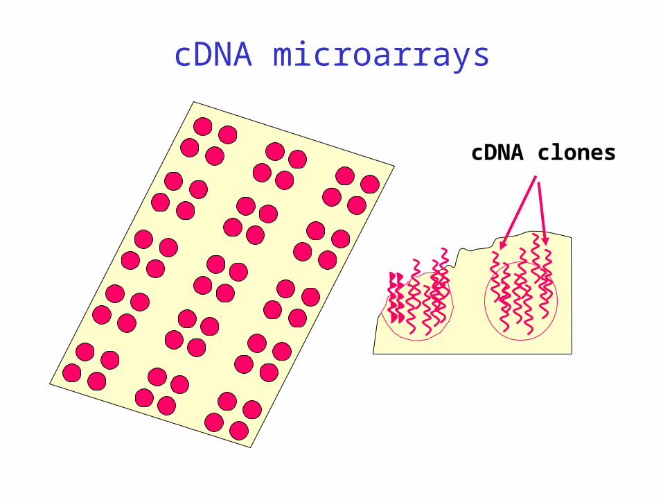
cDNA microarrays
cDNA clones
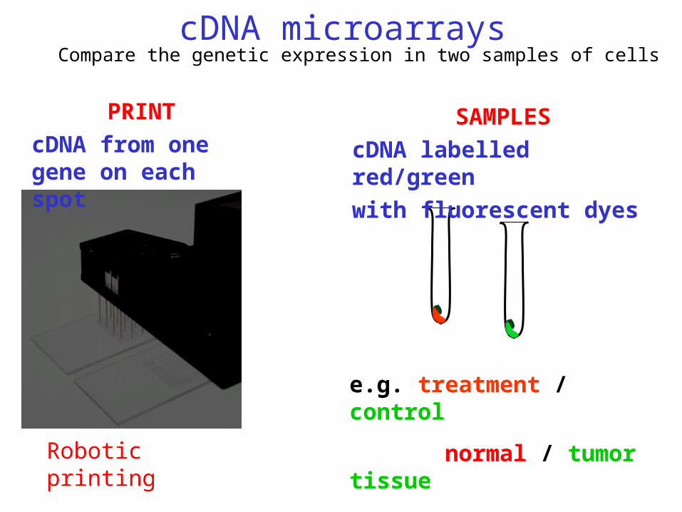
cDNA microarraysCompare the genetic expression in two samples of cells
cDNA from one gene on each spot
SAMPLES
cDNA labelled red/green
with fluorescent dyes
e.g. treatment / control
normal / tumor tissueRobotic printing
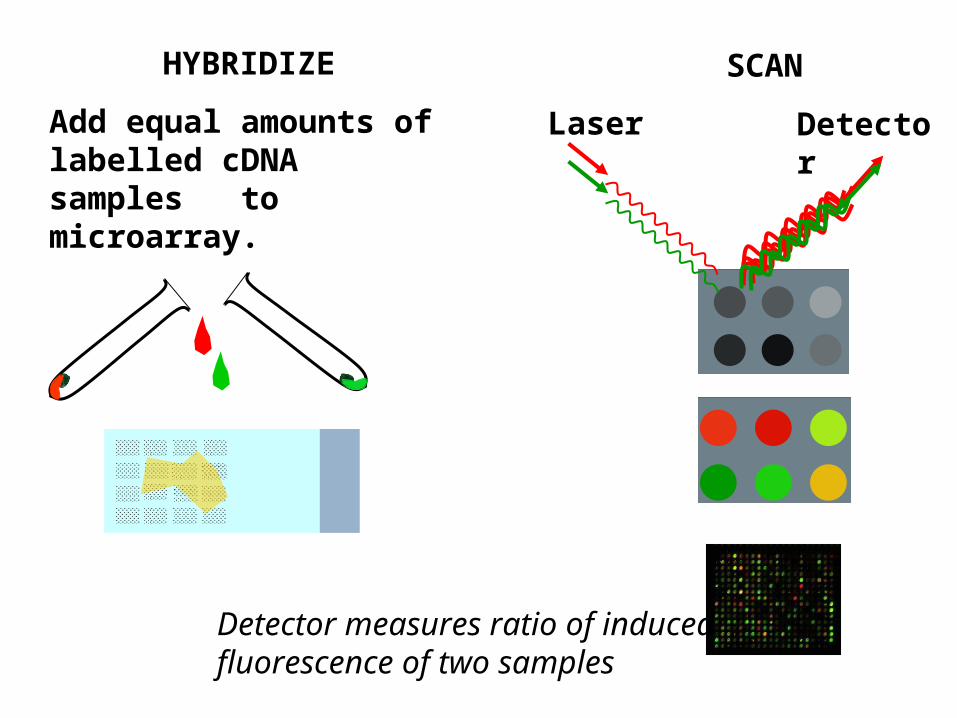
HYBRIDIZE
Add equal amounts of labelled cDNA samples to microarray.
SCAN
Laser Detector
Detector measures ratio of induced fluorescence of two samples
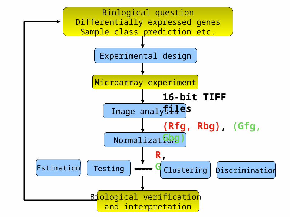
Biological questionDifferentially expressed genesSample class prediction etc.
Testing
Biological verification and interpretation
Microarray experiment
Estimation
Experimental design
Image analysis
Normalization
Clustering Discrimination
R, G
16-bit TIFF files
(Rfg, Rbg), (Gfg, Gbg)
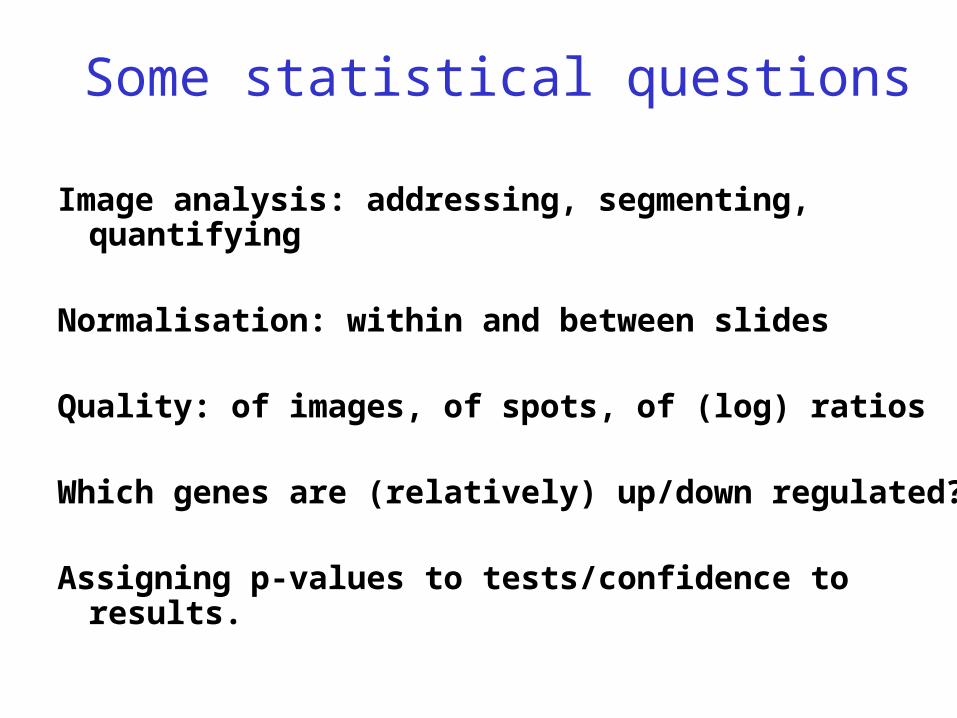
Some statistical questions
Image analysis: addressing, segmenting, quantifying Normalisation: within and between slides
Quality: of images, of spots, of (log) ratios
Which genes are (relatively) up/down regulated?
Assigning p-values to tests/confidence to results.
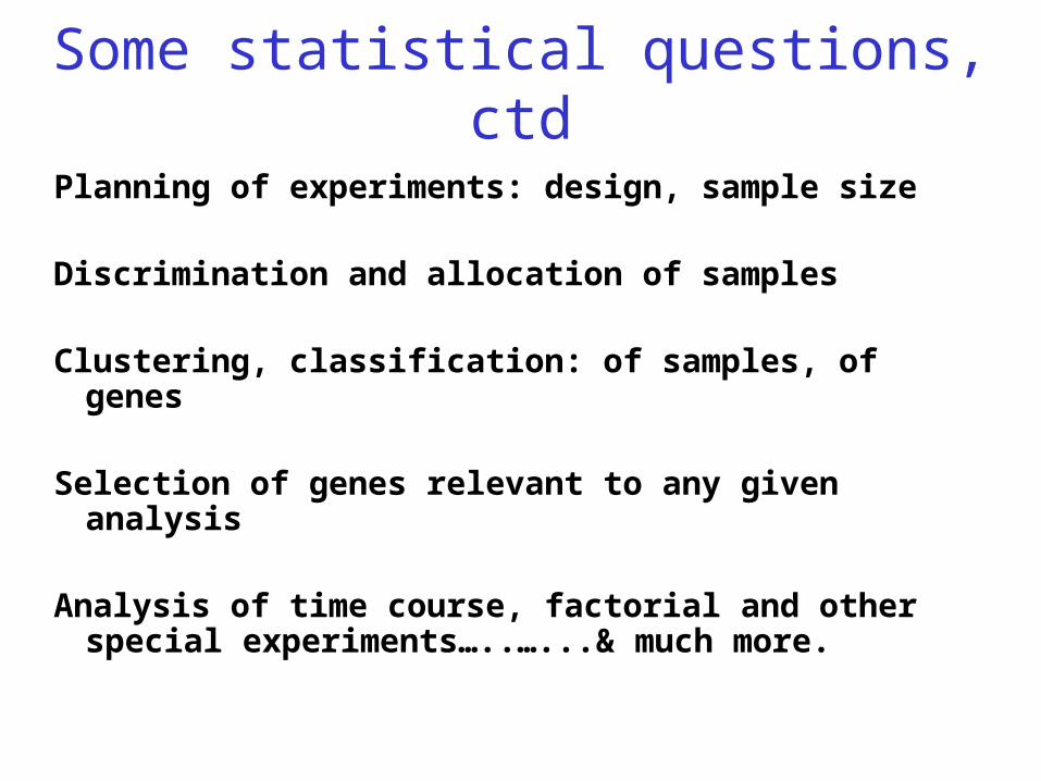
Some statistical questions, ctd
Planning of experiments: design, sample size
Discrimination and allocation of samples
Clustering, classification: of samples, of genes
Selection of genes relevant to any given analysis
Analysis of time course, factorial and other special experiments…..…...& much more.
Some bioinformatic questions
Connecting spots to databases, e.g. to sequence, structure, and pathway databases
Discovering short sequences regulating sets of genes: direct and inverse methods
Relating expression profiles to structure and function, e.g. protein localisation
Identifying novel biochemical or signalling pathways, ………..and much more.
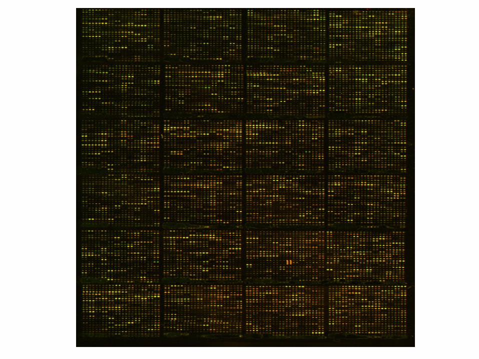
Some basic problems….
…with automatically scanning the microarrays
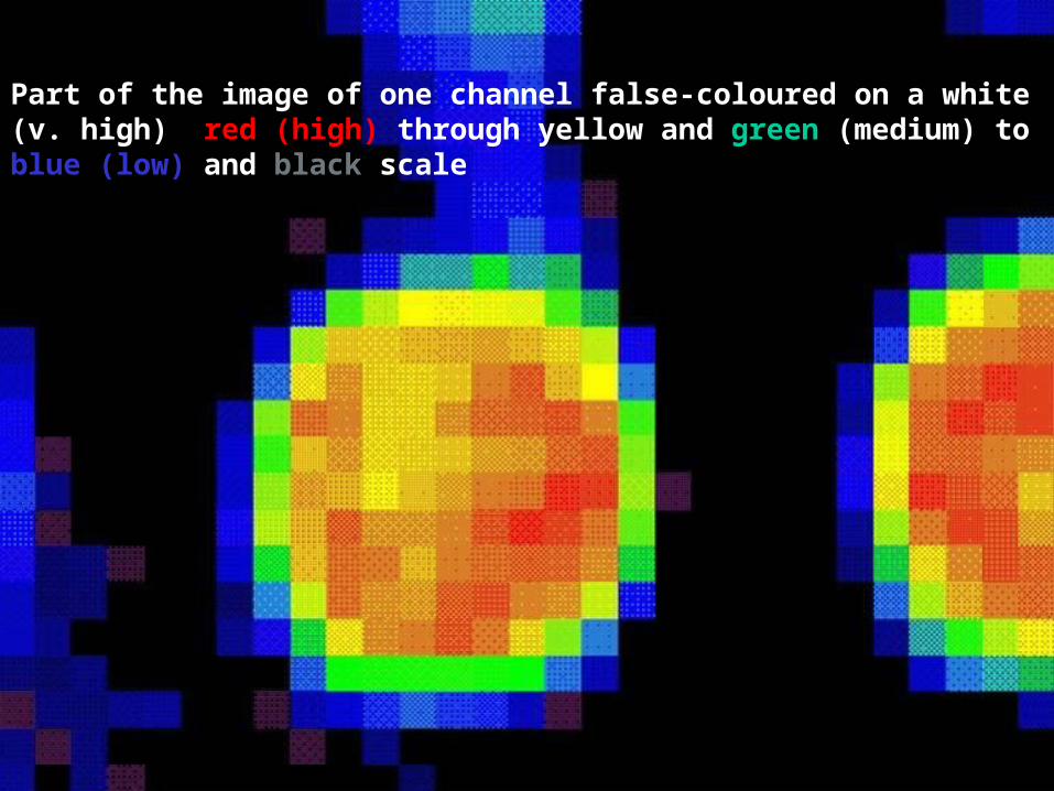
Part of the image of one channel false-coloured on a white (v. high) red (high) through yellow and green (medium) to blue (low) and black scale
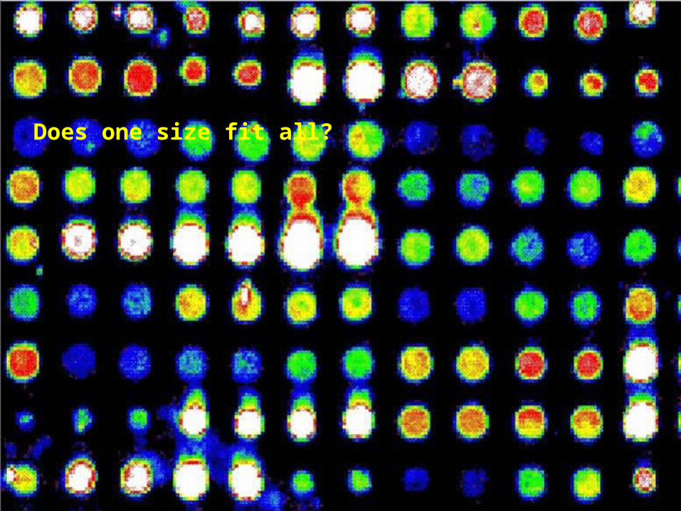
Does one size fit all?
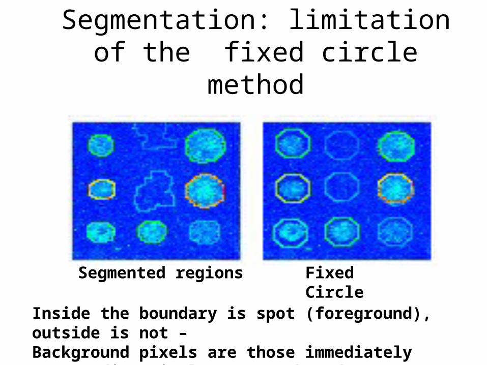
Segmentation: limitation of the fixed circle method
Segmented regions Fixed Circle
Inside the boundary is spot (foreground), outside is not – Background pixels are those immediately surrounding circle/segment boundary
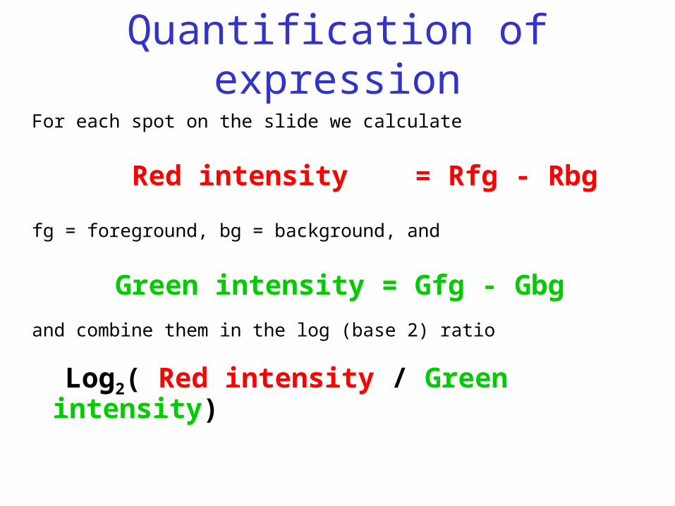
Quantification of expression
For each spot on the slide we calculate
Red intensity = Rfg - Rbg
fg = foreground, bg = background, and
Green intensity = Gfg - Gbg
and combine them in the log (base 2) ratio
Log2( Red intensity / Green intensity)
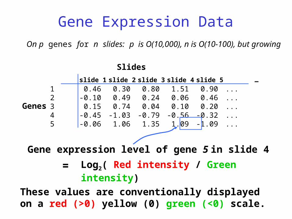
Gene Expression Data
On p genes for n slides: p is O(10,000), n is O(10-100), but growing
Genes
Slides
Gene expression level of gene 5 in slide 4
= Log2( Red intensity / Green intensity)
slide 1 slide 2 slide 3 slide 4 slide 5 …
1 0.46 0.30 0.80 1.51 0.90 ...2 -0.10 0.49 0.24 0.06 0.46 ...3 0.15 0.74 0.04 0.10 0.20 ...4 -0.45 -1.03 -0.79 -0.56 -0.32 ...5 -0.06 1.06 1.35 1.09 -1.09 ...
These values are conventionally displayed on a red (>0) yellow (0) green (<0) scale.
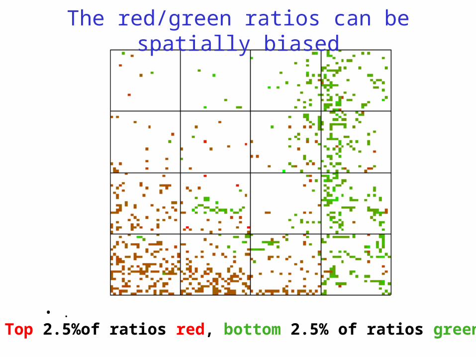
The red/green ratios can be spatially biased
• .Top 2.5%of ratios red, bottom 2.5% of ratios green
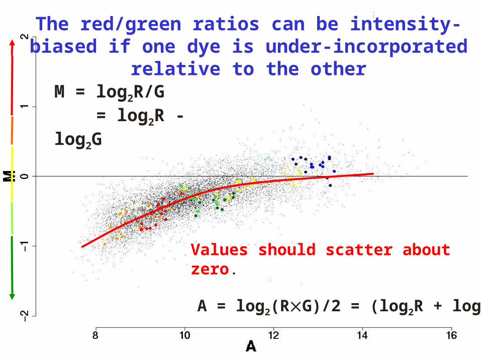
The red/green ratios can be intensity-biased if one dye is under-incorporated relative to the other
M = log2R/G = log2R - log2G
A = log2(RG)/2 = (log2R + log2G)/2
Values should scatter about zero.
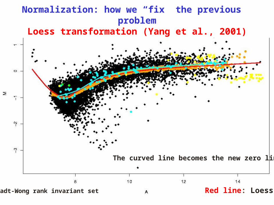
Orange: Schadt-Wong rank invariant set Red line: Loess smooth
Normalization: how we “fix” the previous problemLoess transformation (Yang et al., 2001)
The curved line becomes the new zero line
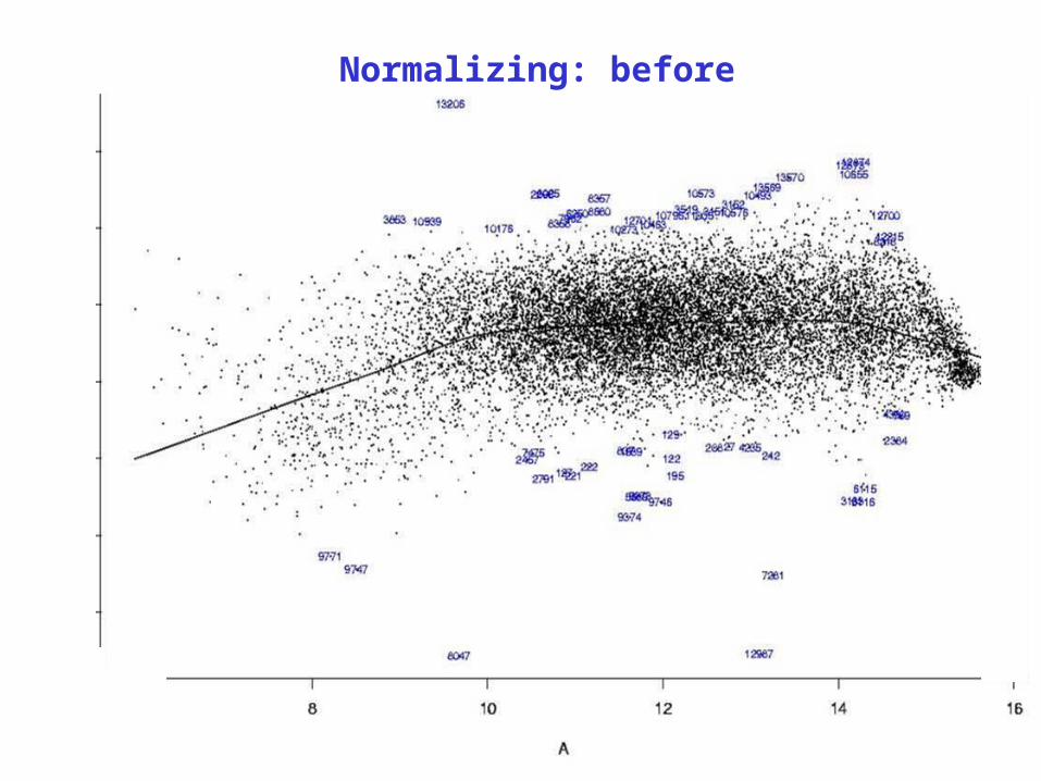
Normalizing: before-4
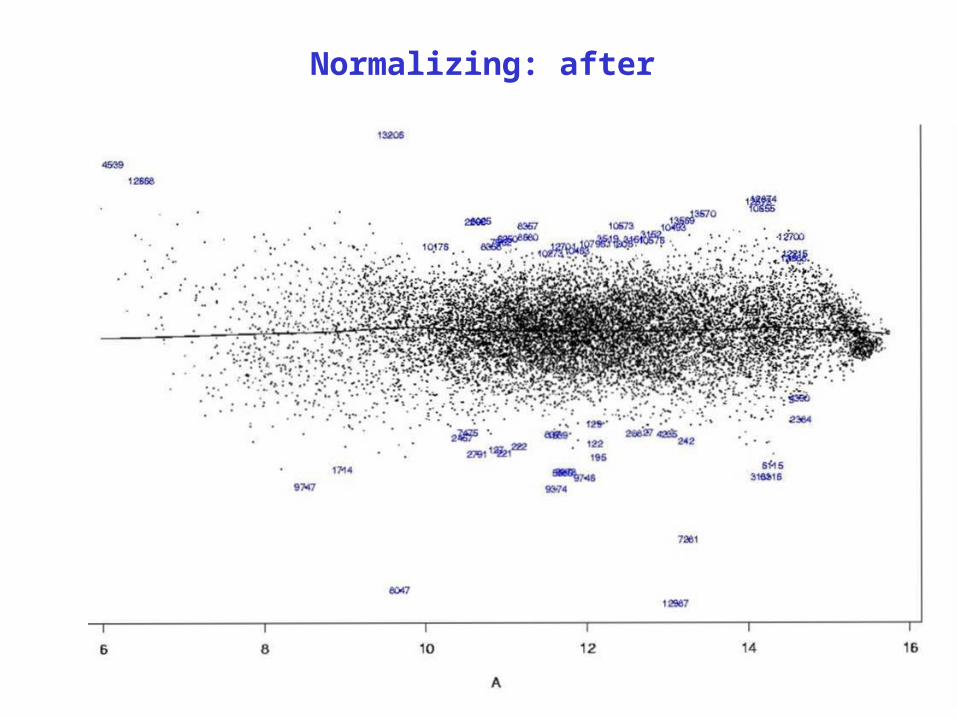
Normalizing: after
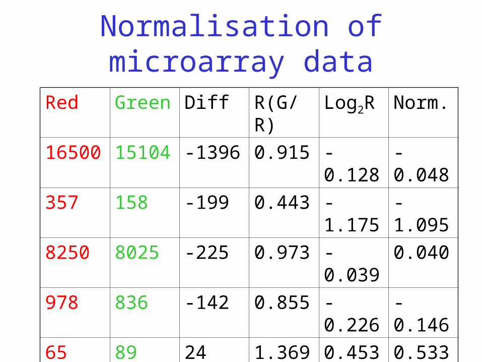
Normalisation of microarray data
Red Green Diff R(G/R) Log2R Norm.
16500 15104 -1396 0.915 -0.128 -0.048
357 158 -199 0.443 -1.175 -1.095
8250 8025 -225 0.973 -0.039 0.040
978 836 -142 0.855 -0.226 -0.146
65 89 24 1.369 0.453 0.533
684 1368 539 2.000 1.000 1.080
13772 11209 -2563 0.814 -0.297 -0.217
856 731 -125 0.854 -0.228 -0.148
Analysis of Variance (ANOVA) approach
• ANOVA is a robust statistical procedure• Partitions sources of variation, e.g. whether
variation in gene expression is less in subset of data than in total data set
• Requires moderate levels of replication (4-10 replicates of each treatment)
• But no reference sample needed• Expression judged according to statistical
significance instead of by adopting arbitrary thresholds
Analysis of Variance (ANOVA) approachhas two steps
• Raw fluorescence data is log-transformed and arrays and dye channels are normalised with respect to one another. You get normalised expression levels where dye and array effects are eliminated
• A second model is fit to normalised expression levels associated with each individual gene
Analysis of Variance (ANOVA) approach
• Advantage: design does not need reference samples• Concern: treatments should be randomised and all
single differences between treatments should be covered
E.g., if male kidney and female liver are contrasted on one set, and female kidney and male liver on another, we cannot state whether gender or tissue type is responsible for expression differences observed
Analysis of Variance (ANOVA) experimental microarray setups
• Loop design of experiments possible: A-B, B-C, C-D, and D-A
• Flipping of dyes (dye swap) to filter artifacts due to preferential labeling
• Completely or partially randomised designs
Dye swap
• Repeating hybridization on two-dye microarrays with the same samples but swapped fluorescent labels.
• For example, sample A is labeled with Cy3 (green) and sample B with Cy5 (red) in the first array, but sample A is labeled with Cy5 and sample B with Cy3 in the second array.
• Dye swap is used to remove technical colour bias in some genes. Dye swap is a technical replication (=subreplication).
Analysis of Variance (ANOVA)
• Within-array variance among replicated clones is much lower than between-array variance, due to stoichiometry of labeling during reverse transcription
• So do not duplicate spots on same array, this renders effects seemingly large
Oligonucleotide arrays
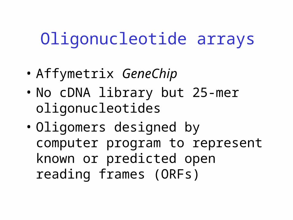
• Affymetrix GeneChip
• No cDNA library but 25-mer oligonucleotides
• Oligomers designed by computer program to represent known or predicted open reading frames (ORFs)
Oligonucleotide arrays
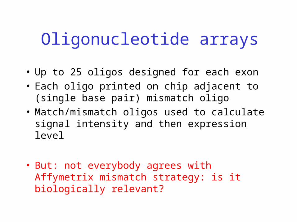
• Up to 25 oligos designed for each exon • Each oligo printed on chip adjacent to (single base
pair) mismatch oligo• Match/mismatch oligos used to calculate signal
intensity and then expression level
• But: not everybody agrees with Affymetrix mismatch strategy: is it biologically relevant?
Oligonucleotide arrays
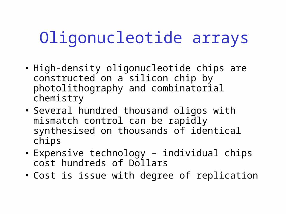
• High-density oligonucleotide chips are constructed on a silicon chip by photolithography and combinatorial chemistry
• Several hundred thousand oligos with mismatch control can be rapidly synthesised on thousands of identical chips
• Expensive technology – individual chips cost hundreds of Dollars
• Cost is issue with degree of replication
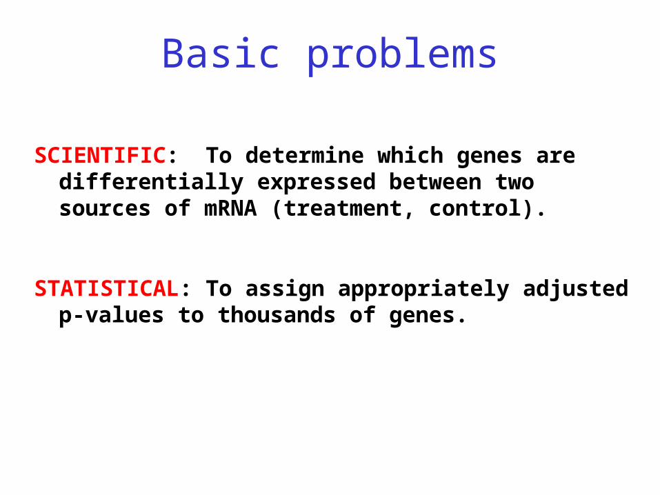
SCIENTIFIC: To determine which genes are differentially expressed between two sources of mRNA (treatment, control).
STATISTICAL: To assign appropriately adjusted p-values to thousands of genes.
Basic problems
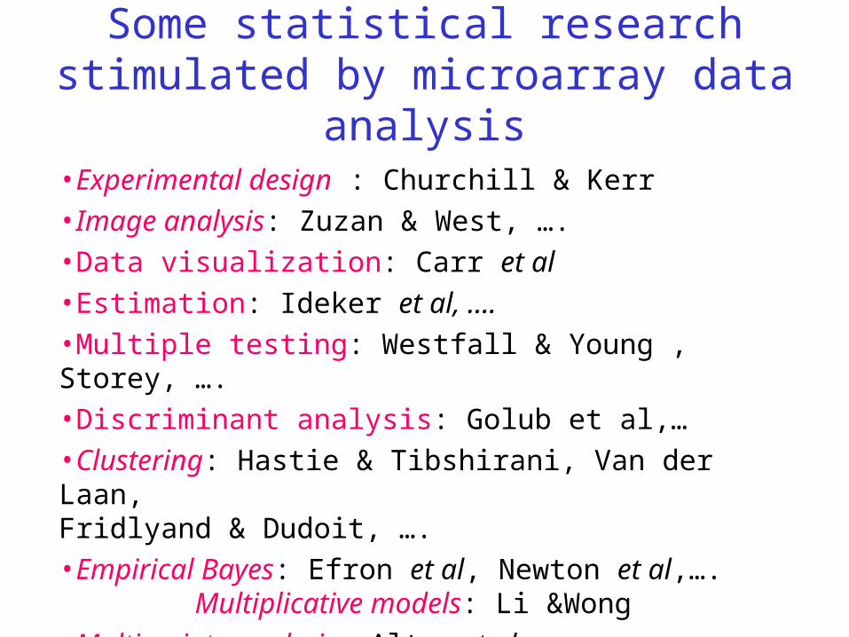
Some statistical research stimulated by microarray data analysis
•Experimental design : Churchill & Kerr
•Image analysis: Zuzan & West, ….
•Data visualization: Carr et al
•Estimation: Ideker et al, ….
•Multiple testing: Westfall & Young , Storey, ….
•Discriminant analysis: Golub et al,…
•Clustering: Hastie & Tibshirani, Van der Laan, Fridlyand & Dudoit, ….
•Empirical Bayes: Efron et al, Newton et al,…. Multiplicative models: Li &Wong
•Multivariate analysis: Alter et al
•Genetic networks: D’Haeseleer et al and more
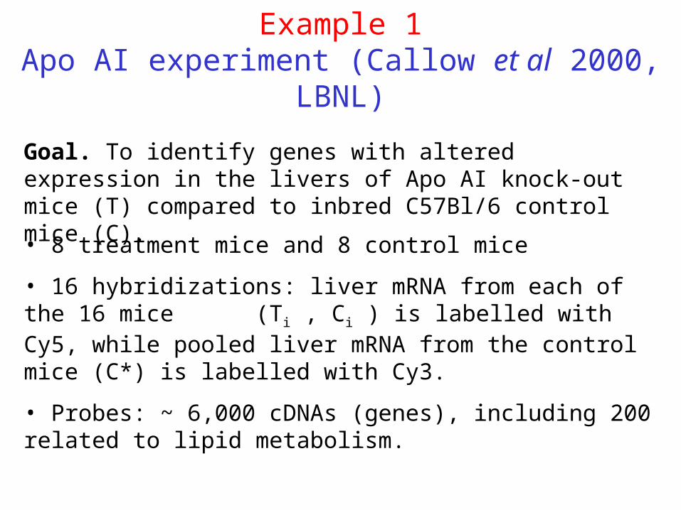
• 8 treatment mice and 8 control mice
• 16 hybridizations: liver mRNA from each of the 16 mice (Ti , Ci ) is labelled with Cy5, while pooled liver mRNA from the control mice (C*) is labelled with Cy3.
• Probes: ~ 6,000 cDNAs (genes), including 200 related to lipid metabolism.
Goal. To identify genes with altered expression in the livers of Apo AI knock-out mice (T) compared to inbred C57Bl/6 control mice (C).
Example 1Apo AI experiment (Callow et al 2000, LBNL)
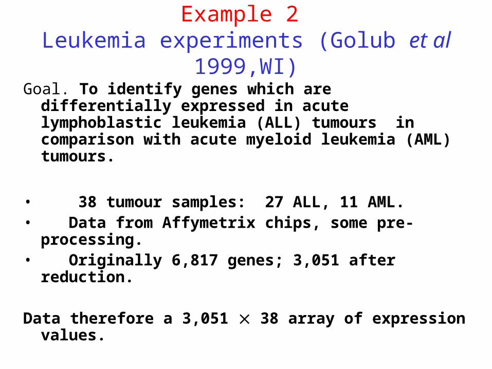
Example 2 Leukemia experiments (Golub et al 1999,WI)
Goal. To identify genes which are differentially expressed in acute lymphoblastic leukemia (ALL) tumours in comparison with acute myeloid leukemia (AML) tumours.
• 38 tumour samples: 27 ALL, 11 AML.• Data from Affymetrix chips, some pre-processing.• Originally 6,817 genes; 3,051 after reduction.
Data therefore a 3,051 38 array of expression values.