gene finding and - tau
TRANSCRIPT
Gene finding and regulatory motif analysis
December 20, 2016
גנומיקה חישובית , חיים וולפסון' פרופ, רון שמיר' פרופ
ויקס -עירית גת' דר אוניברסיטת תל אביב ,ס למדעי המחשב"ביה
Computational Genomics Prof. Ron Shamir, Prof. Haim Wolfson, Dr. Irit Gat-Viks
School of Computer Science, Tel Aviv University
Gene Finding
Sources: •Lecture notes of Larry Ruzzo, UW. •Slides by Nir Friedman, Hebrew U. •Burge, Karlin: “Finding Genes in Genomic DNA”, Curr. Opin. In Struct. Biol 8(3) ’98 • Slides by Chuong Huynh on Gene Prediction, NCBI •Durbin’s book, Ch. 3 •Pevzner’s book, Ch. 9
2
CG © Ron Shamir
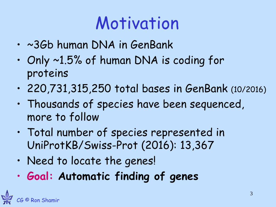
Motivation • ~3Gb human DNA in GenBank
• Only ~1.5% of human DNA is coding for proteins
• 220,731,315,250 total bases in GenBank (10/2016)
• Thousands of species have been sequenced, more to follow
• Total number of species represented in UniProtKB/Swiss-Prot (2016): 13,367
• Need to locate the genes!
• Goal: Automatic finding of genes
3
CG © Ron Shamir
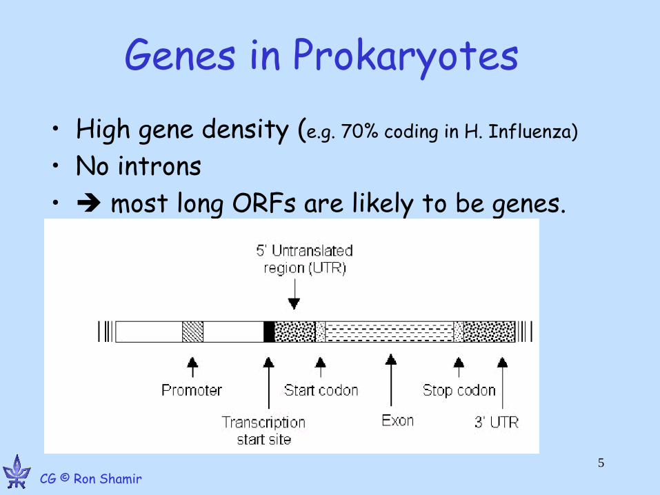
Genes in Prokaryotes
• High gene density (e.g. 70% coding in H. Influenza)
• No introns
• most long ORFs are likely to be genes.
5
CG © Ron Shamir
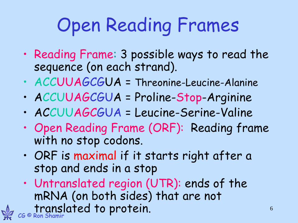
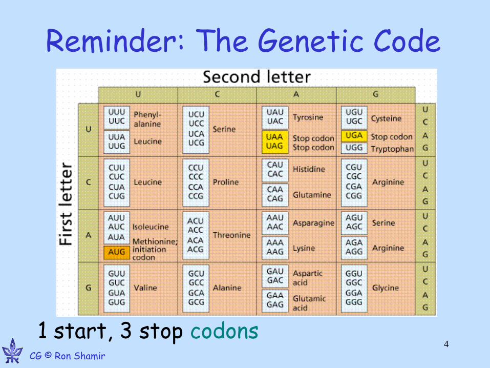
Open Reading Frames
• Reading Frame: 3 possible ways to read the sequence (on each strand).
• ACCUUAGCGUA = Threonine-Leucine-Alanine
• ACCUUAGCGUA = Proline-Stop-Arginine • ACCUUAGCGUA = Leucine-Serine-Valine • Open Reading Frame (ORF): Reading frame
with no stop codons. • ORF is maximal if it starts right after a
stop and ends in a stop • Untranslated region (UTR): ends of the
mRNA (on both sides) that are not translated to protein.
CG © Ron Shamir 6
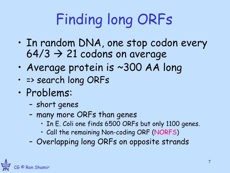
Finding long ORFs
• In random DNA, one stop codon every 64/3 21 codons on average
• Average protein is ~300 AA long • => search long ORFs
• Problems: – short genes – many more ORFs than genes
• In E. Coli one finds 6500 ORFs but only 1100 genes. • Call the remaining Non-coding ORF (NORFS)
– Overlapping long ORFs on opposite strands
7
CG © Ron Shamir
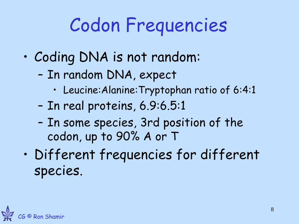
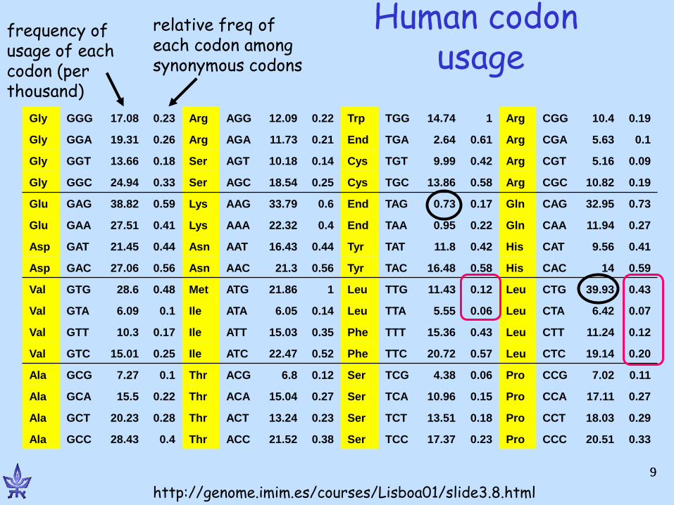
Codon Frequencies
• Coding DNA is not random: – In random DNA, expect
• Leucine:Alanine:Tryptophan ratio of 6:4:1
– In real proteins, 6.9:6.5:1
– In some species, 3rd position of the codon, up to 90% A or T
• Different frequencies for different species.
8
CG © Ron Shamir
9
Human codon usage
Gly GGG 17.08 0.23 Arg AGG 12.09 0.22 Trp TGG 14.74 1 Arg CGG 10.4 0.19
Gly GGA 19.31 0.26 Arg AGA 11.73 0.21 End TGA 2.64 0.61 Arg CGA 5.63 0.1
Gly GGT 13.66 0.18 Ser AGT 10.18 0.14 Cys TGT 9.99 0.42 Arg CGT 5.16 0.09
Gly GGC 24.94 0.33 Ser AGC 18.54 0.25 Cys TGC 13.86 0.58 Arg CGC 10.82 0.19
Glu GAG 38.82 0.59 Lys AAG 33.79 0.6 End TAG 0.73 0.17 Gln CAG 32.95 0.73
Glu GAA 27.51 0.41 Lys AAA 22.32 0.4 End TAA 0.95 0.22 Gln CAA 11.94 0.27
Asp GAT 21.45 0.44 Asn AAT 16.43 0.44 Tyr TAT 11.8 0.42 His CAT 9.56 0.41
Asp GAC 27.06 0.56 Asn AAC 21.3 0.56 Tyr TAC 16.48 0.58 His CAC 14 0.59
Val GTG 28.6 0.48 Met ATG 21.86 1 Leu TTG 11.43 0.12 Leu CTG 39.93 0.43
Val GTA 6.09 0.1 Ile ATA 6.05 0.14 Leu TTA 5.55 0.06 Leu CTA 6.42 0.07
Val GTT 10.3 0.17 Ile ATT 15.03 0.35 Phe TTT 15.36 0.43 Leu CTT 11.24 0.12
Val GTC 15.01 0.25 Ile ATC 22.47 0.52 Phe TTC 20.72 0.57 Leu CTC 19.14 0.20
Ala GCG 7.27 0.1 Thr ACG 6.8 0.12 Ser TCG 4.38 0.06 Pro CCG 7.02 0.11
Ala GCA 15.5 0.22 Thr ACA 15.04 0.27 Ser TCA 10.96 0.15 Pro CCA 17.11 0.27
Ala GCT 20.23 0.28 Thr ACT 13.24 0.23 Ser TCT 13.51 0.18 Pro CCT 18.03 0.29
Ala GCC 28.43 0.4 Thr ACC 21.52 0.38 Ser TCC 17.37 0.23 Pro CCC 20.51 0.33
http://genome.imim.es/courses/Lisboa01/slide3.8.html
frequency of usage of each codon (per thousand)
relative freq of each codon among synonymous codons
9
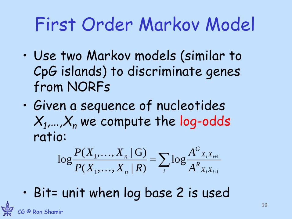
First Order Markov Model
• Use two Markov models (similar to CpG islands) to discriminate genes from NORFs
• Given a sequence of nucleotides X1,…,Xn we compute the log-odds ratio:
• Bit= unit when log base 2 is used
i XX
R
XXG
n
n
ii
ii
A
A
RXXP
XXP
1
1log)|,,(
)G|,,(log
1
1
10
CG © Ron Shamir
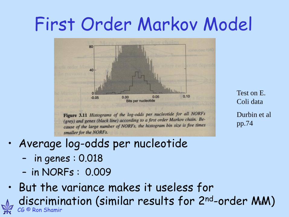
First Order Markov Model
• Average log-odds per nucleotide – in genes : 0.018
– in NORFs : 0.009
• But the variance makes it useless for discrimination (similar results for 2nd-order MM)
Test on E.
Coli data
Durbin et al
pp.74
11
CG © Ron Shamir
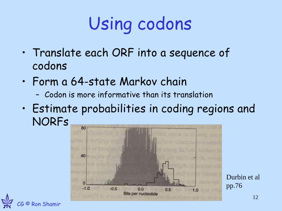
Using codons
• Translate each ORF into a sequence of codons
• Form a 64-state Markov chain – Codon is more informative than its translation
• Estimate probabilities in coding regions and NORFs
Durbin et al
pp.76
12
CG © Ron Shamir
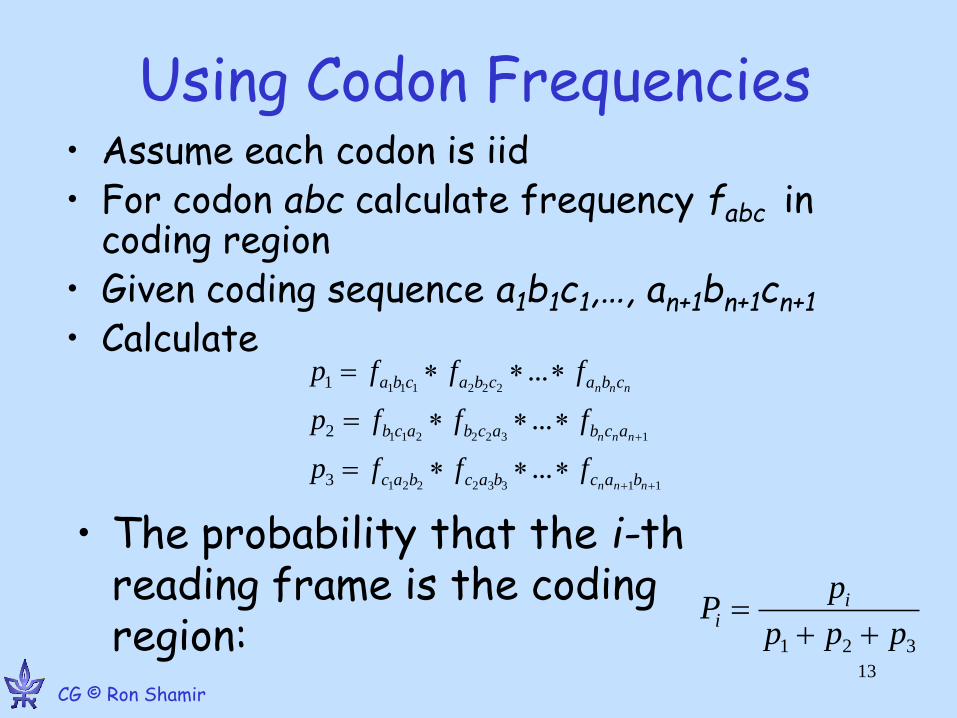
Using Codon Frequencies
• The probability that the i-th reading frame is the coding region:
11332221
1322211
222111
...
...
...
3
2
1
nnn
nnn
nnn
bacbacbac
acbacbacb
cbacbacba
fffp
fffp
fffp
321 ppp
pP i
i
• Assume each codon is iid • For codon abc calculate frequency fabc in
coding region • Given coding sequence a1b1c1,…, an+1bn+1cn+1 • Calculate
13
CG © Ron Shamir
CodonPreference
ORF
The real genes
Sliding window length (in codons)
FR
AM
E 1
F
RA
ME
2
FR
AM
E 3
14
CG © Ron Shamir
RNA Transcription
• Not all ORFs are expressed. • Transcription depends on regulatory signals • Minimal regulatory region – core promoter
to which RNA polymerase and initiation factors bind to start transcription.
• At the termination signal the polymerase releases the RNA and disconnects from the DNA.
15
CG © Ron Shamir
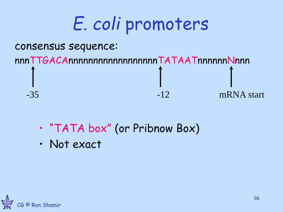
E. coli promoters
• “TATA box” (or Pribnow Box)
• Not exact
consensus sequence: nnnTTGACAnnnnnnnnnnnnnnnnnnTATAATnnnnnnNnnn
-35 -12 mRNA start
16
CG © Ron Shamir
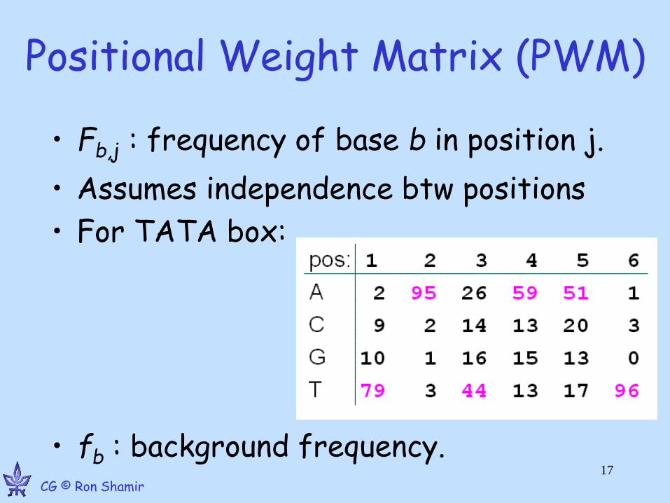
Positional Weight Matrix (PWM)
• Fb,j : frequency of base b in position j.
• Assumes independence btw positions
• For TATA box:
• fb : background frequency.
17
CG © Ron Shamir
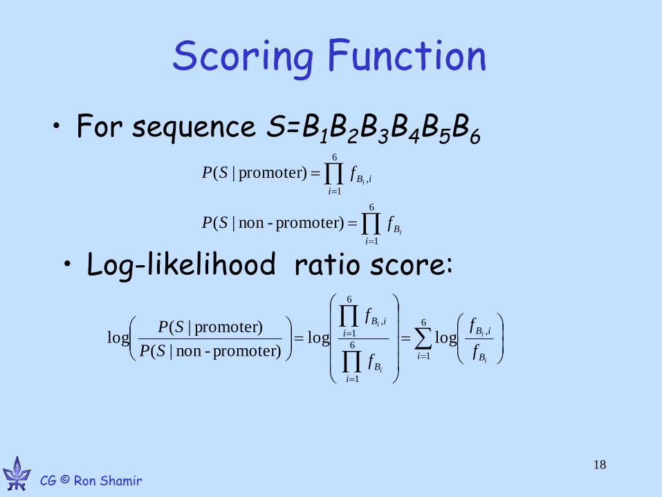
Scoring Function
• For sequence S=B1B2B3B4B5B6
6
1
6
1
,
)promoter-non|(
)promoter|(
i
B
i
iB
i
i
fSP
fSP
6
1
,
6
1
6
1
,
loglog)promoter-non|(
)promoter|(log
i B
iB
i
B
i
iB
i
i
i
i
f
f
f
f
SP
SP
• Log-likelihood ratio score:
18
CG © Ron Shamir
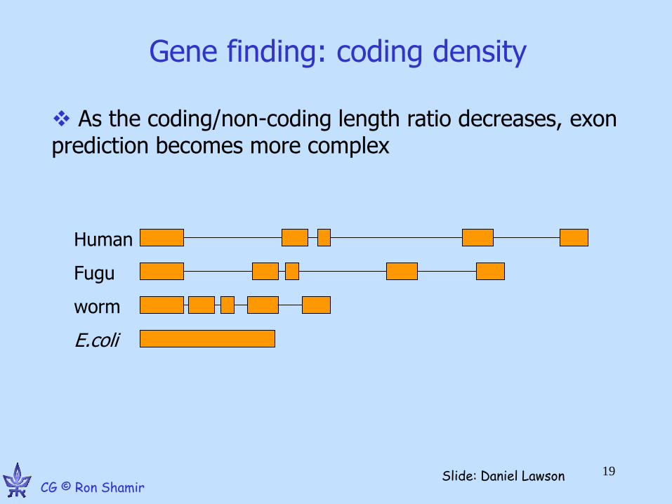
Gene finding: coding density
As the coding/non-coding length ratio decreases, exon prediction becomes more complex
Human
Fugu
worm
E.coli
19
CG © Ron Shamir Slide: Daniel Lawson
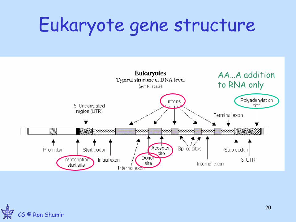
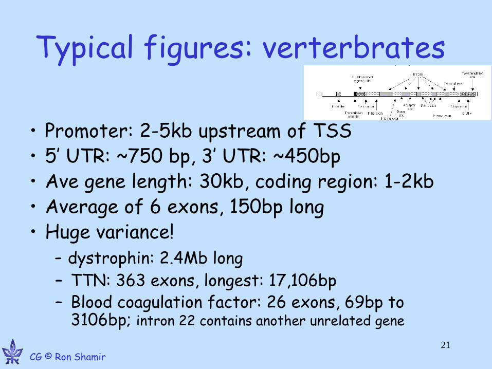
Typical figures: verterbrates
• Promoter: 2-5kb upstream of TSS • 5’ UTR: ~750 bp, 3’ UTR: ~450bp • Ave gene length: 30kb, coding region: 1-2kb • Average of 6 exons, 150bp long • Huge variance!
- dystrophin: 2.4Mb long
– TTN: 363 exons, longest: 17,106bp – Blood coagulation factor: 26 exons, 69bp to
3106bp; intron 22 contains another unrelated gene
21
CG © Ron Shamir
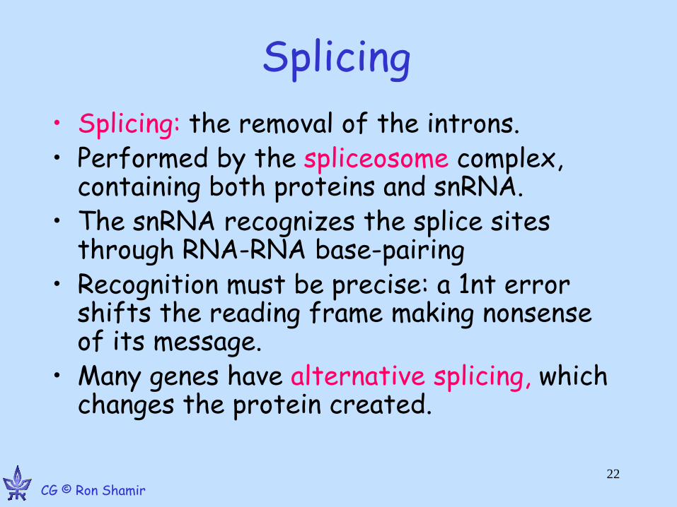
Splicing
• Splicing: the removal of the introns. • Performed by the spliceosome complex,
containing both proteins and snRNA. • The snRNA recognizes the splice sites
through RNA-RNA base-pairing • Recognition must be precise: a 1nt error
shifts the reading frame making nonsense of its message.
• Many genes have alternative splicing, which changes the protein created.
22
CG © Ron Shamir
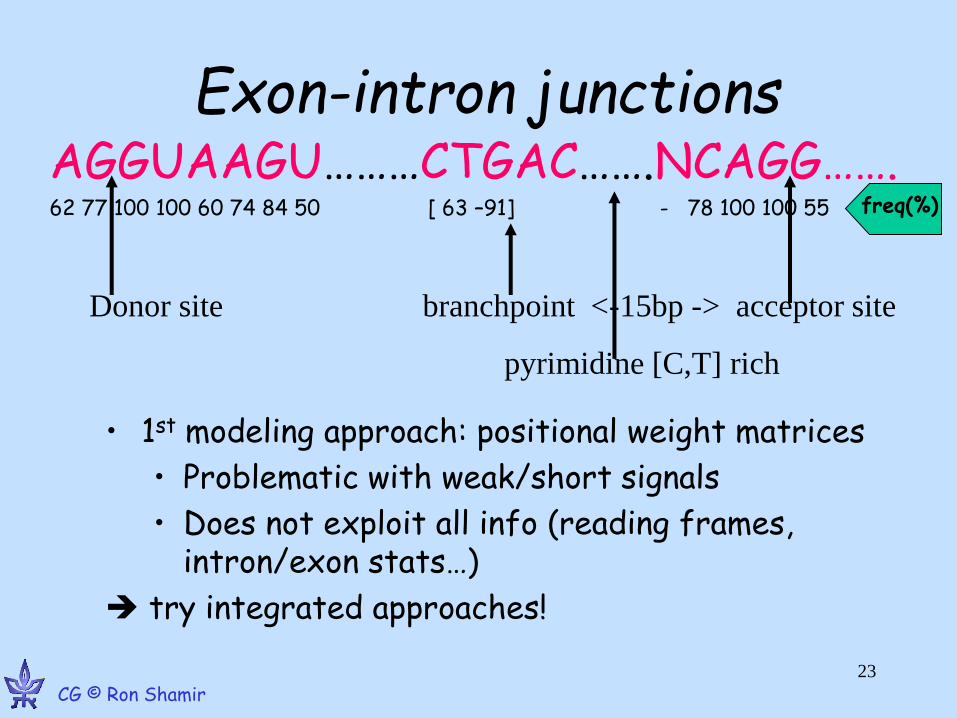
Exon-intron junctions
• 1st modeling approach: positional weight matrices
• Problematic with weak/short signals
• Does not exploit all info (reading frames, intron/exon stats…)
try integrated approaches!
AGGUAAGU………CTGAC…….NCAGG……. 62 77 100 100 60 74 84 50 [ 63 –91] - 78 100 100 55
Donor site branchpoint <-15bp -> acceptor site
pyrimidine [C,T] rich
freq(%)
23
CG © Ron Shamir
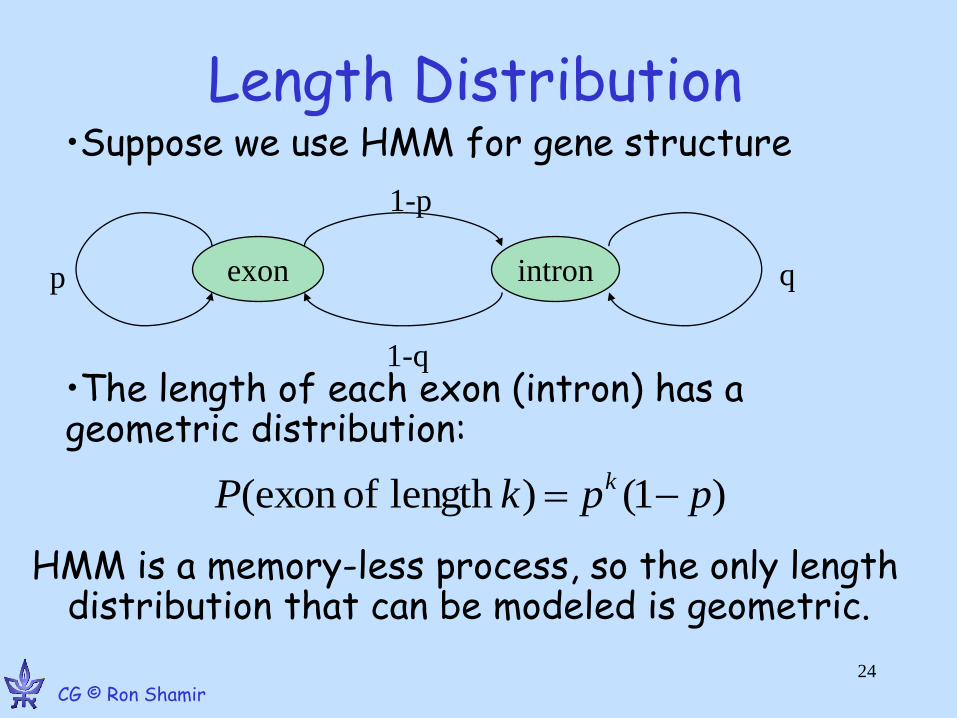
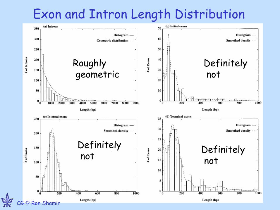
Length Distribution
HMM is a memory-less process, so the only length distribution that can be modeled is geometric.
exon intron p q
1-p
1-q
)1()length ofexon ( ppkP k
•Suppose we use HMM for gene structure
•The length of each exon (intron) has a geometric distribution:
24
CG © Ron Shamir
25
CG © Ron Shamir
Exon and Intron Length Distribution
Roughly geometric
Definitely not
Definitely not
Definitely not
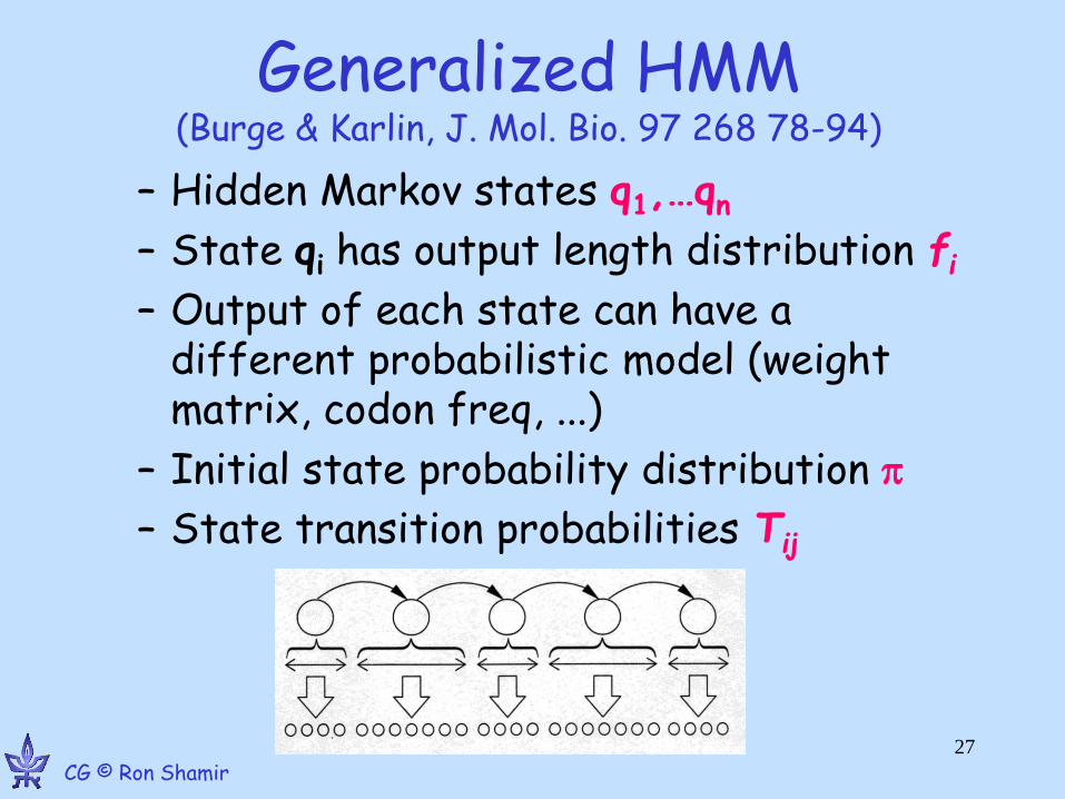
Generalized HMM (Burge & Karlin, J. Mol. Bio. 97 268 78-94)
– Hidden Markov states q1,…qn
– State qi has output length distribution fi
– Output of each state can have a different probabilistic model (weight matrix, codon freq, ...)
– Initial state probability distribution
– State transition probabilities Tij
27
CG © Ron Shamir
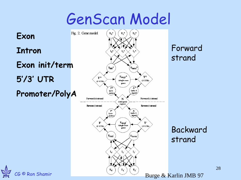
GenScan Model Exon
Intron
Exon init/term
5’/3’ UTR
Promoter/PolyA
Forward strand
Backward strand
Burge & Karlin JMB 97
28
CG © Ron Shamir
GenScan model
• states = functional units along a gene
• The allowed transitions ensure the order is biologically consistent
• The index of the intron model = the phase of the exons before and after it
• In terms of output and length, I0,I1,I2 are identical
29
CG © Ron Shamir
ACCUUAGCGUA …intron…. ACCUUAGCGUA
ACCUUAGCGUA …intron…. ACCUUAGCGUA
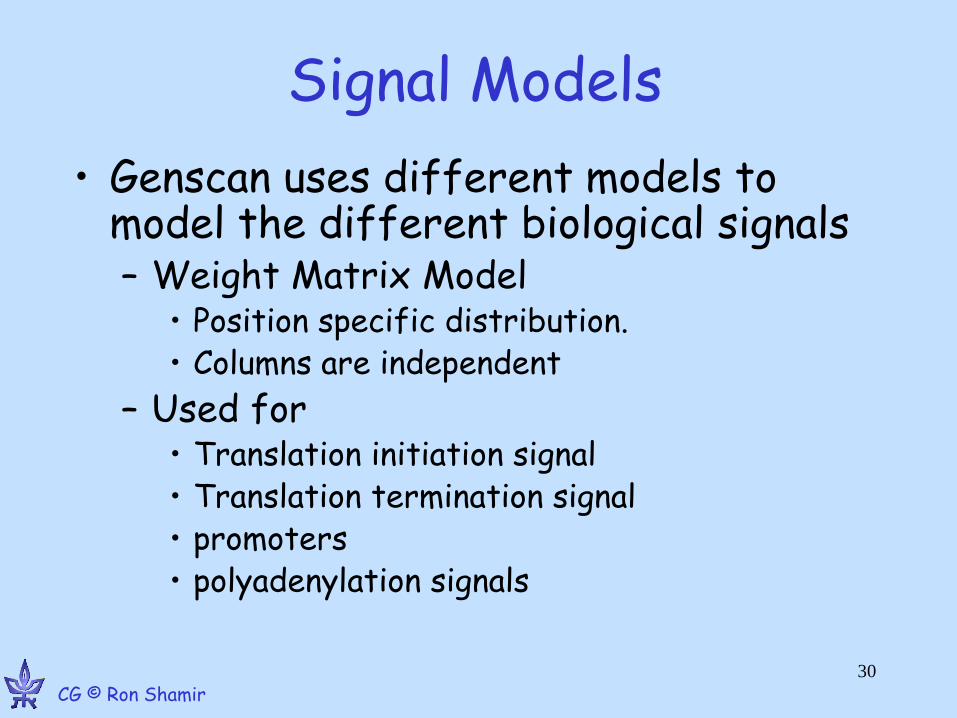
Signal Models
• Genscan uses different models to model the different biological signals – Weight Matrix Model
• Position specific distribution. • Columns are independent
– Used for • Translation initiation signal • Translation termination signal • promoters • polyadenylation signals
CG © Ron Shamir 30
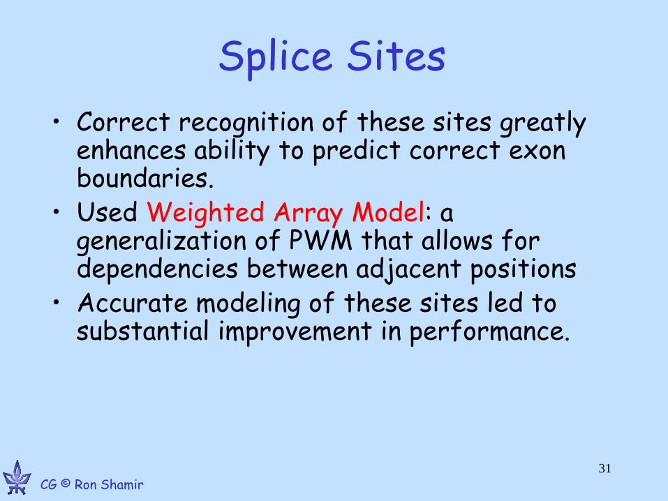
Splice Sites
• Correct recognition of these sites greatly enhances ability to predict correct exon boundaries.
• Used Weighted Array Model: a generalization of PWM that allows for dependencies between adjacent positions
• Accurate modeling of these sites led to substantial improvement in performance.
31
CG © Ron Shamir
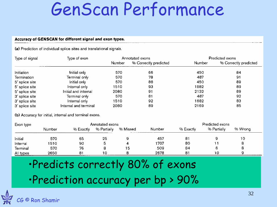
GenScan Performance
•Predicts correctly 80% of exons
•Prediction accuracy per bp > 90% 32
CG © Ron Shamir

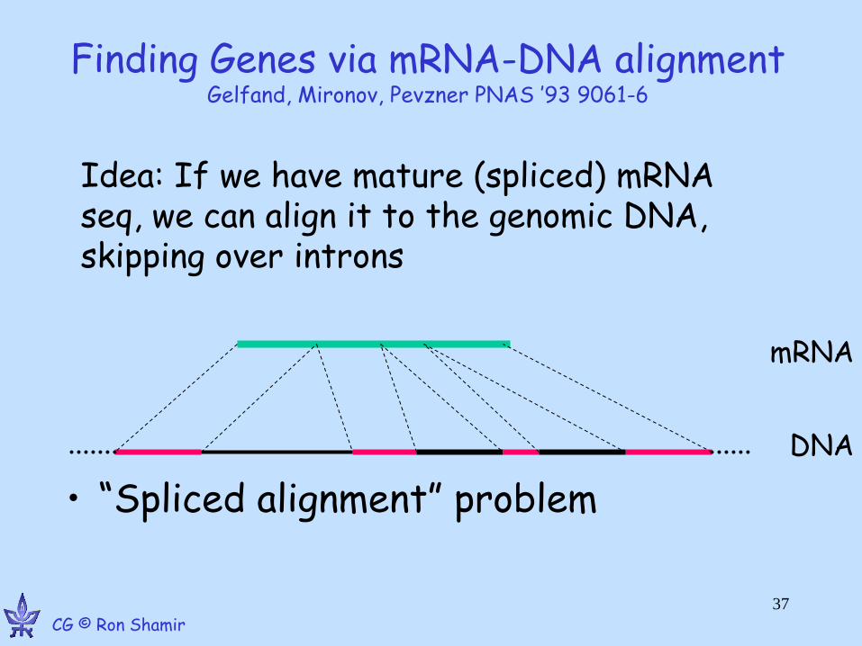
Finding Genes via mRNA-DNA alignment Gelfand, Mironov, Pevzner PNAS ’93 9061-6
• “Spliced alignment” problem
Idea: If we have mature (spliced) mRNA seq, we can align it to the genomic DNA, skipping over introns
CG © Ron Shamir 37
DNA
mRNA
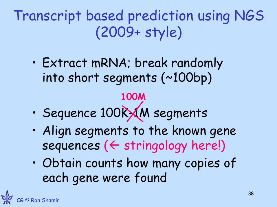
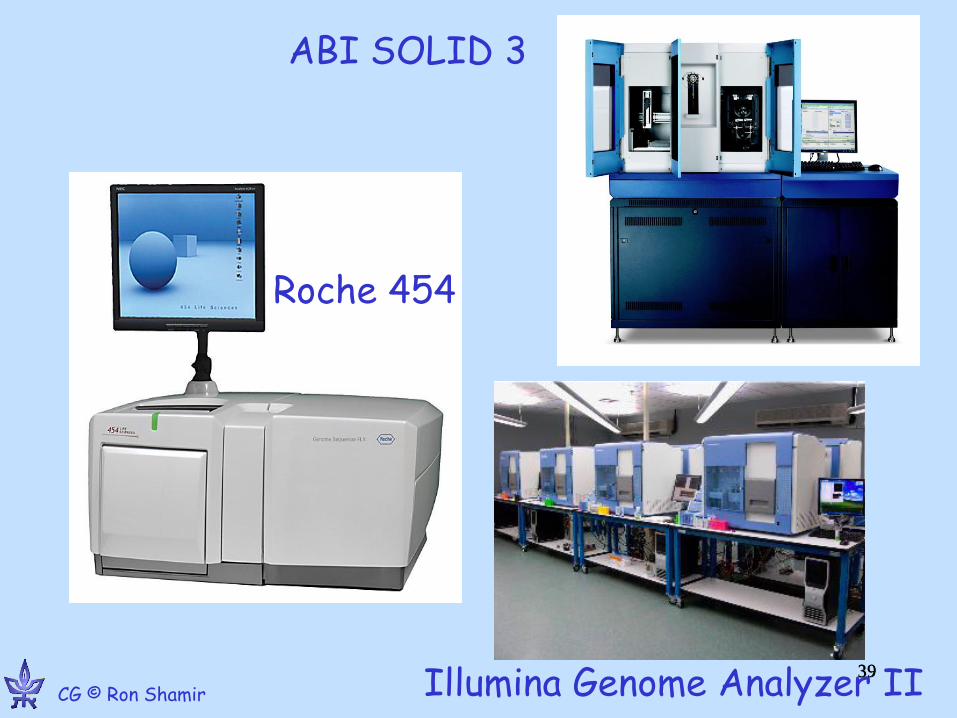
Transcript based prediction using NGS (2009+ style)
• Extract mRNA; break randomly into short segments (~100bp)
• Sequence 100K-1M segments
• Align segments to the known gene sequences ( stringology here!)
• Obtain counts how many copies of each gene were found
38
100M
CG © Ron Shamir 38
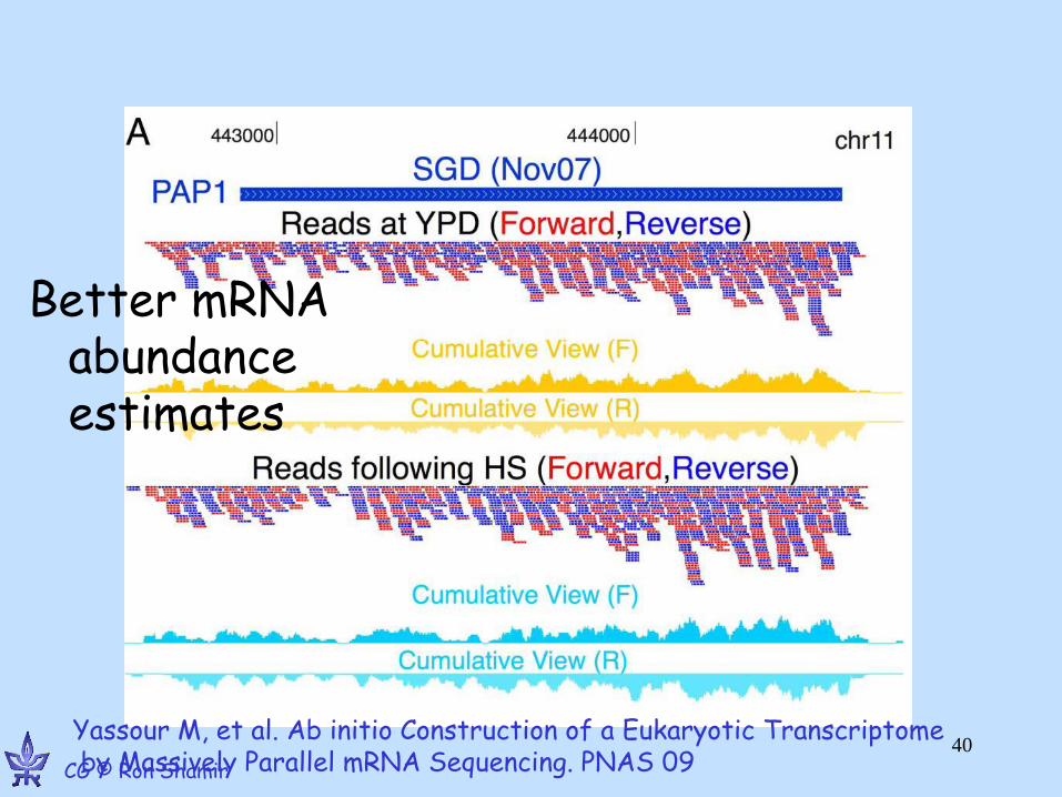
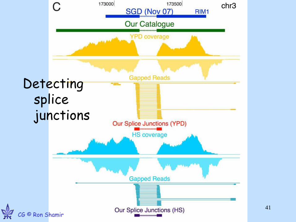
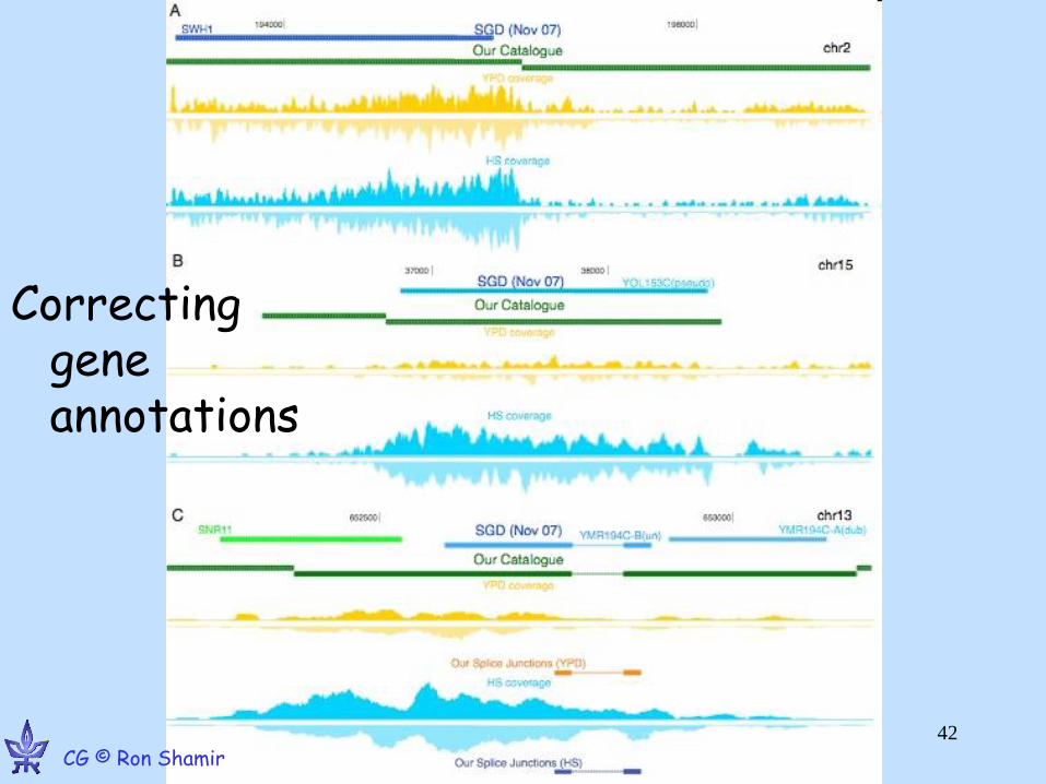
Yassour M, et al. Ab initio Construction of a Eukaryotic Transcriptome by Massively Parallel mRNA Sequencing. PNAS 09 CG © Ron Shamir
40
Better mRNA abundance estimates
GE © Ron Shamir •44
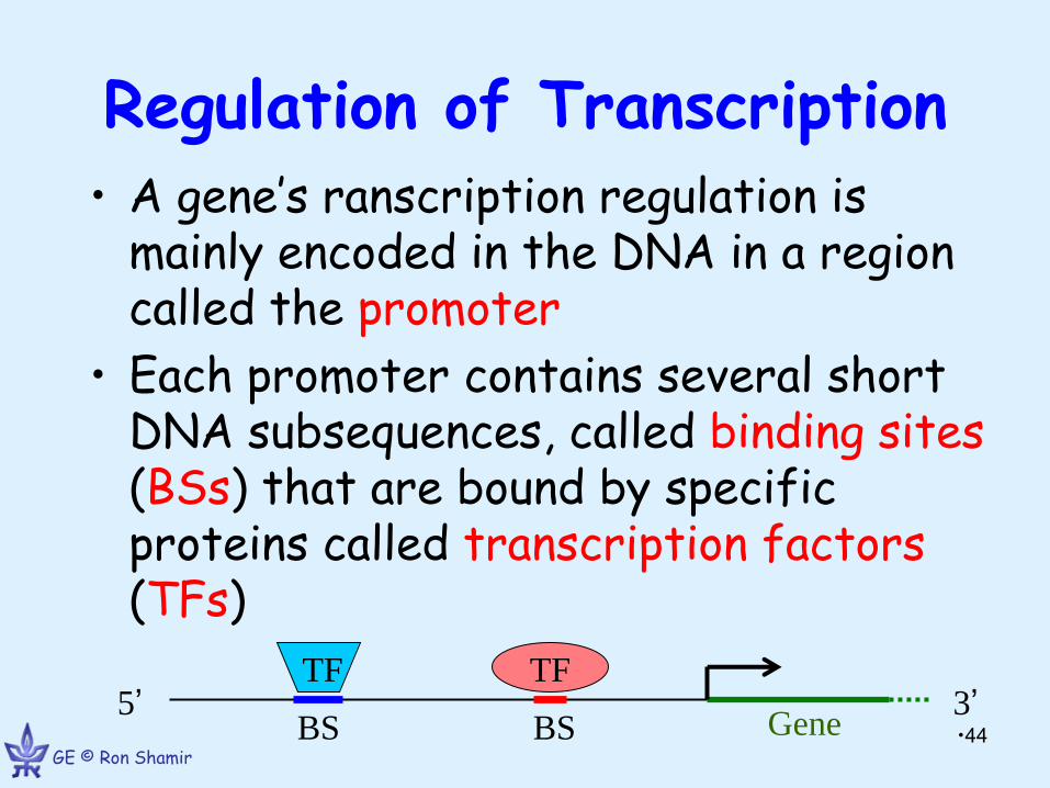
Regulation of Transcription • A gene’s ranscription regulation is
mainly encoded in the DNA in a region called the promoter
• Each promoter contains several short DNA subsequences, called binding sites (BSs) that are bound by specific proteins called transcription factors (TFs)
TF TF
Gene 5’ 3’
BS BS
GE © Ron Shamir •45
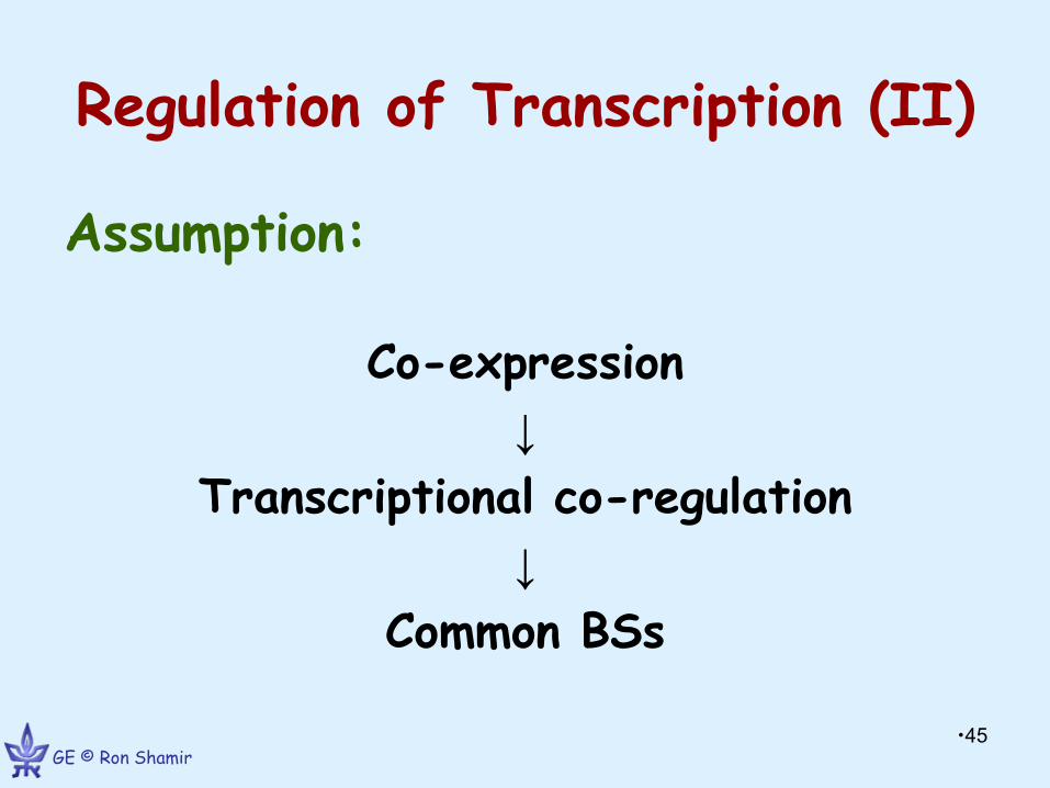
Regulation of Transcription (II)
Assumption:
Co-expression
↓
Transcriptional co-regulation
↓
Common BSs
GE © Ron Shamir •46
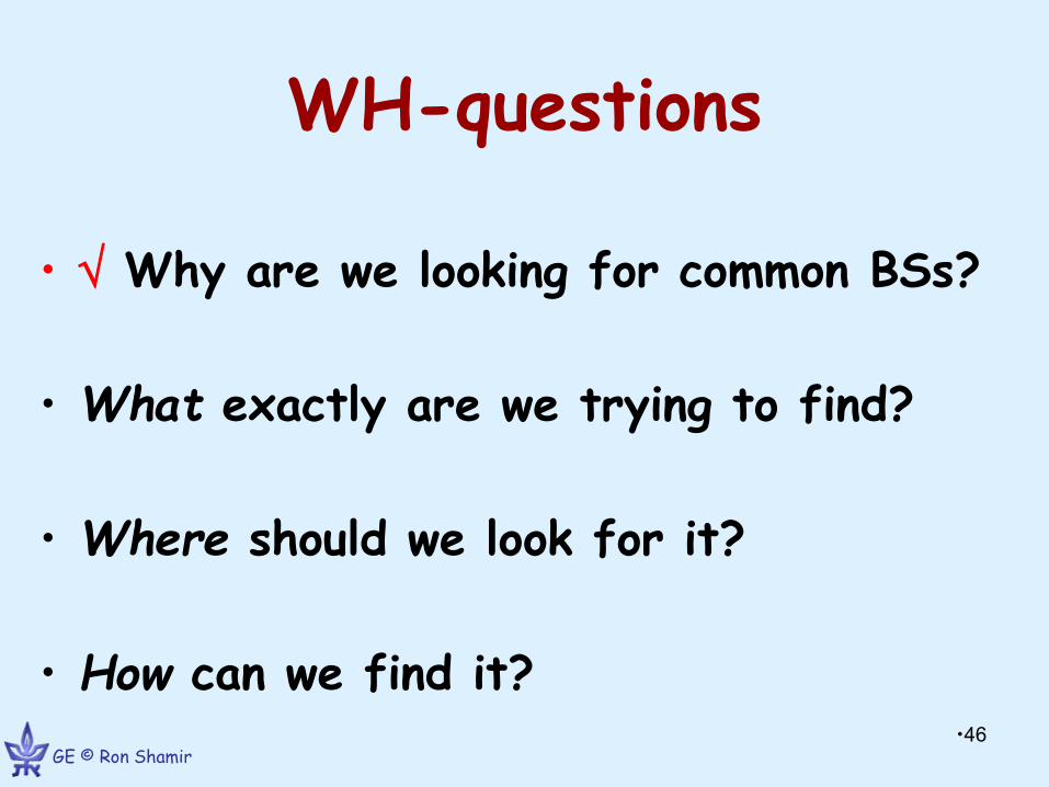
WH-questions
• Why are we looking for common BSs?
• What exactly are we trying to find?
• Where should we look for it?
• How can we find it?
GE © Ron Shamir •47
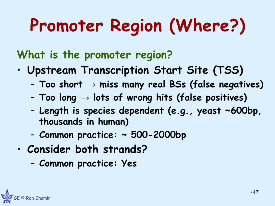
Promoter Region (Where?)
What is the promoter region?
• Upstream Transcription Start Site (TSS) – Too short → miss many real BSs (false negatives)
– Too long → lots of wrong hits (false positives)
– Length is species dependent (e.g., yeast ~600bp, thousands in human)
– Common practice: ~ 500-2000bp
• Consider both strands? – Common practice: Yes

What: Models for Binding Sites
•48
GE © Ron Shamir •49
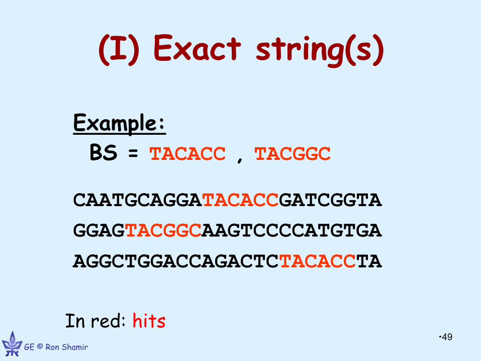
(I) Exact string(s)
Example:
BS = TACACC , TACGGC
CAATGCAGGATACACCGATCGGTA
GGAGTACGGCAAGTCCCCATGTGA
AGGCTGGACCAGACTCTACACCTA
In red: hits
GE © Ron Shamir •50
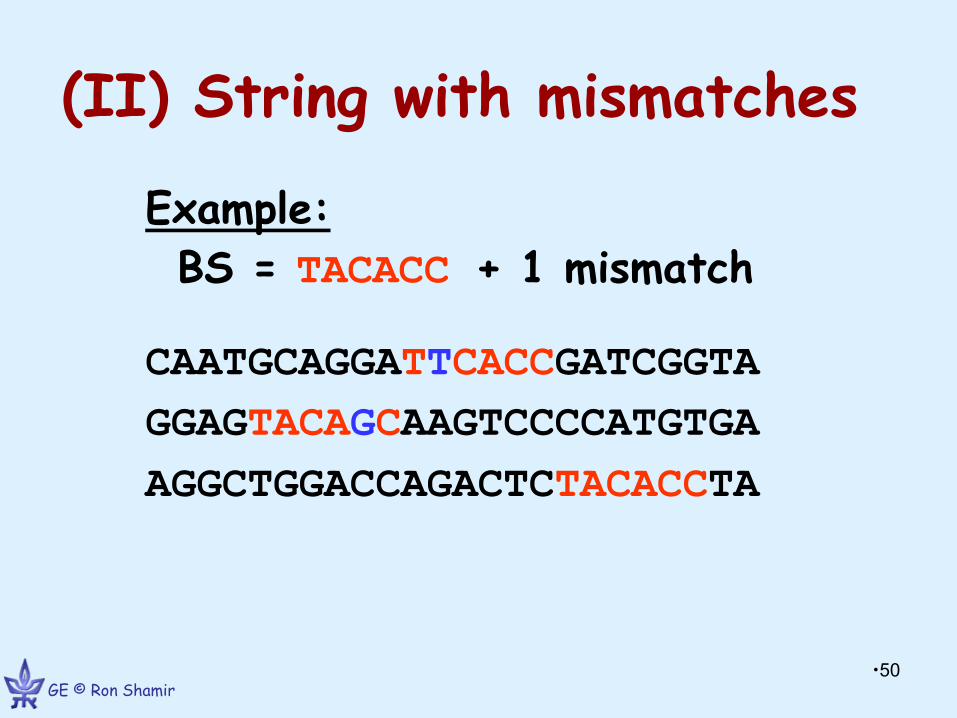
(II) String with mismatches
Example:
BS = TACACC + 1 mismatch
CAATGCAGGATTCACCGATCGGTA
GGAGTACAGCAAGTCCCCATGTGA
AGGCTGGACCAGACTCTACACCTA
GE © Ron Shamir •51
(III) Degenerate string
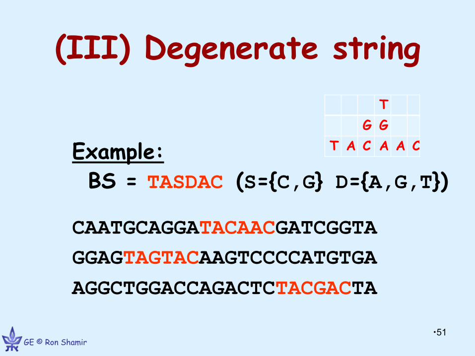
Example:
BS = TASDAC (S={C,G} D={A,G,T})
CAATGCAGGATACAACGATCGGTA
GGAGTAGTACAAGTCCCCATGTGA
AGGCTGGACCAGACTCTACGACTA
T
G G
T A C A A C
GE © Ron Shamir •52
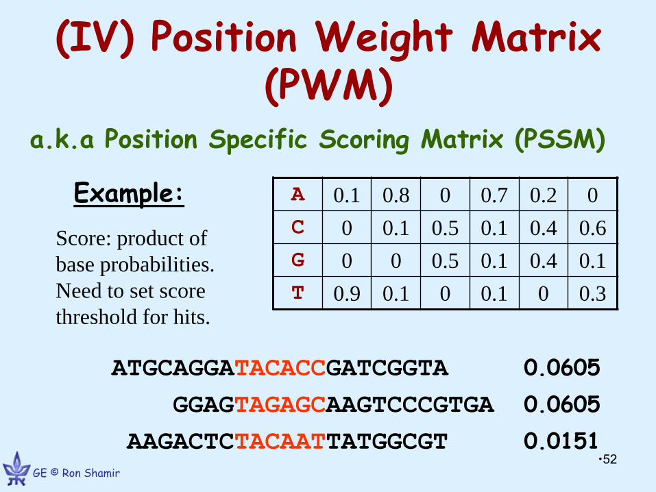
(IV) Position Weight Matrix (PWM)
a.k.a Position Specific Scoring Matrix (PSSM)
Example:
0 0.2 0.7 0 0.8 0.1 A
0.6 0.4 0.1 0.5 0.1 0 C
0.1 0.4 0.1 0.5 0 0 G
0.3 0 0.1 0 0.1 0.9 T
ATGCAGGATACACCGATCGGTA 0.0605
GGAGTAGAGCAAGTCCCGTGA 0.0605
AAGACTCTACAATTATGGCGT 0.0151
Score: product of
base probabilities.
Need to set score
threshold for hits.
How: Experimental techniques
•53
GE © Ron Shamir •54
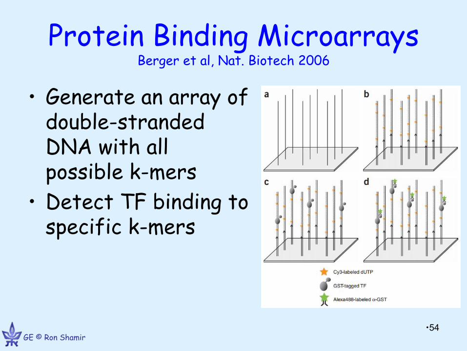
Protein Binding Microarrays Berger et al, Nat. Biotech 2006
• Generate an array of double-stranded DNA with all possible k-mers
• Detect TF binding to specific k-mers
GE © Ron Shamir •55
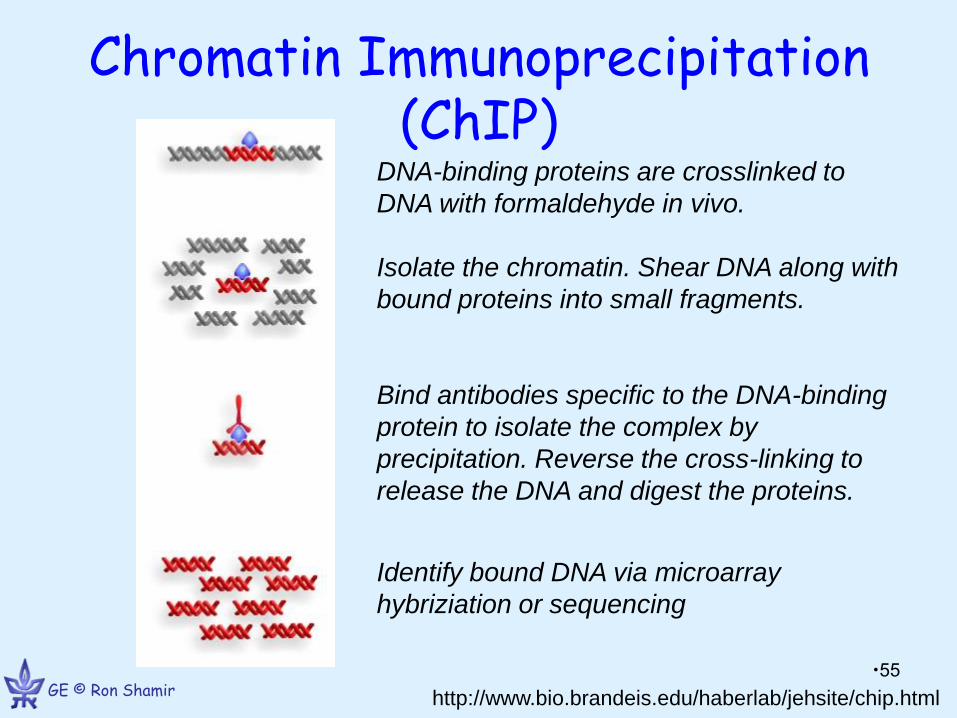
Chromatin Immunoprecipitation (ChIP)
http://www.bio.brandeis.edu/haberlab/jehsite/chip.html
DNA-binding proteins are crosslinked to
DNA with formaldehyde in vivo.
Isolate the chromatin. Shear DNA along with
bound proteins into small fragments.
Bind antibodies specific to the DNA-binding
protein to isolate the complex by
precipitation. Reverse the cross-linking to
release the DNA and digest the proteins.
Identify bound DNA via microarray
hybriziation or sequencing
How: I. Analyzing known motifs
•56
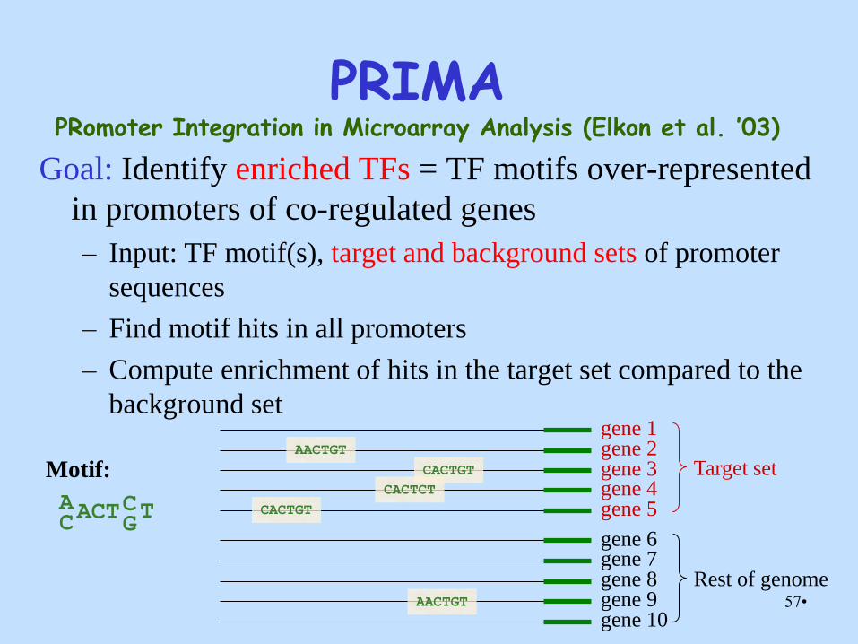
PRIMA PRomoter Integration in Microarray Analysis (Elkon et al. ’03)
Goal: Identify enriched TFs = TF motifs over-represented
in promoters of co-regulated genes
– Input: TF motif(s), target and background sets of promoter
sequences
– Find motif hits in all promoters
– Compute enrichment of hits in the target set compared to the
background set
gene 7
gene 9
gene 5
gene 3 gene 2
gene 4
gene 6
gene 8
gene 10
gene 1
Target set
Rest of genome
C G
A C
T
AACTGT
CACTGT
CACTCT
CACTGT
AACTGT
ACT
Motif:
•57
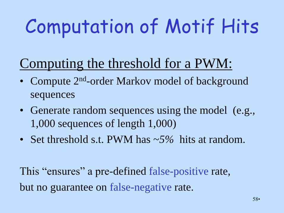
Computation of Motif Hits
Computing the threshold for a PWM:
• Compute 2nd-order Markov model of background
sequences
• Generate random sequences using the model (e.g.,
1,000 sequences of length 1,000)
• Set threshold s.t. PWM has ~5% hits at random.
This “ensures” a pre-defined false-positive rate,
but no guarantee on false-negative rate. •58
Motif Enrichment Each promoter is hit or not.
Let: B = total # of promoters (BG)
T = # of target-set promoters
b = total # of promoters that are hit
t = # of target-set promoters that are hit
Then (hypergeometric distribution assumption):
Prob. for t hits in target-set:
Prob. for at least t hits:
T
B
tT
bB
t
bP(t)
},min{
)(Tb
ti
iPvaluep •59
B
T
t b
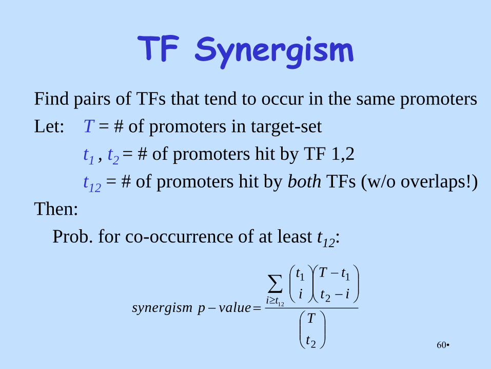
TF Synergism
Find pairs of TFs that tend to occur in the same promoters
Let: T = # of promoters in target-set
t1 , t2 = # of promoters hit by TF 1,2
t12 = # of promoters hit by both TFs (w/o overlaps!)
Then:
Prob. for co-occurrence of at least t12:
2
2
11
12
t
T
it
tT
i
t
valuepsynergismti
•60
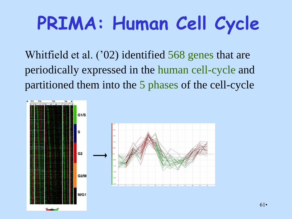
PRIMA: Human Cell Cycle
Whitfield et al. (’02) identified 568 genes that are
periodically expressed in the human cell-cycle and
partitioned them into the 5 phases of the cell-cycle
•61
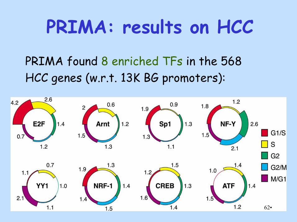
PRIMA: results on HCC
PRIMA found 8 enriched TFs in the 568
HCC genes (w.r.t. 13K BG promoters):
•62
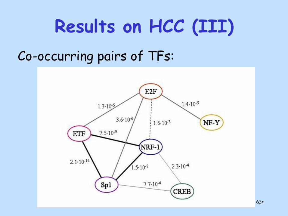
Results on HCC (III)
Co-occurring pairs of TFs:
•63
How: II Motif discovery
•64
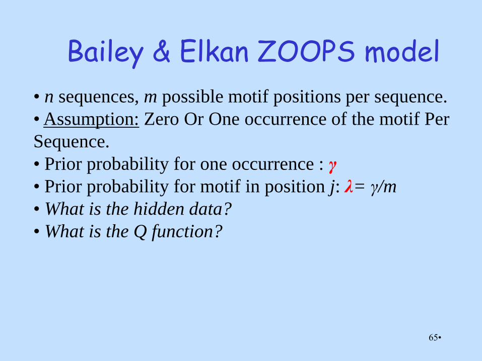
Bailey & Elkan ZOOPS model
• n sequences, m possible motif positions per sequence.
• Assumption: Zero Or One occurrence of the motif Per
Sequence.
• Prior probability for one occurrence : γ
• Prior probability for motif in position j: λ= γ/m
• What is the hidden data?
• What is the Q function?
•65
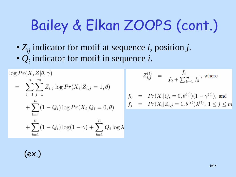
Bailey & Elkan ZOOPS (cont.)
• Zij indicator for motif at sequence i, position j.
• Qi indicator for motif in sequence i.
•66
(ex.)
•CG © Ron Shamir •67
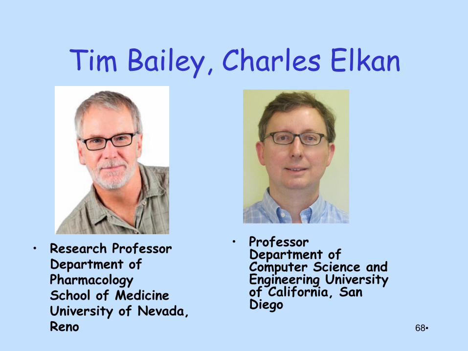
Tim Bailey, Charles Elkan
• Research Professor Department of Pharmacology School of Medicine University of Nevada, Reno
• Professor Department of Computer Science and Engineering University of California, San Diego
•68