general concepts of modeling semiconductor devices

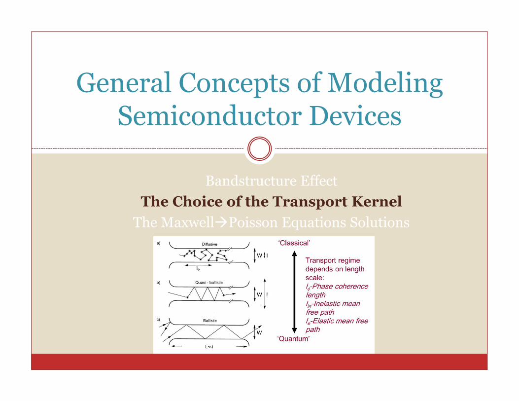
Bandstructure Effect

The Choice of the Transport Kernel

The Maxwell�Poisson Equations Solutions

General Concepts of ModelingSemiconductor Devices

General Device Simulator

D. Vasileska and S.M. Goodnick, Computational Electronics, published by Morgan & Claypool , 2006.D. Vasileska, S. M. Goodnick and G. Klimeck, Computational Electronics: Semi-classical and Quantum Transport Modeling, Taylor & Francis, 2010.

1.

2.3.

Electronic Structure

Advantages of Particular Methods

� Semi-Empirical Methods� Empirical Pseudopotential Method

� Predicts optical gaps

� k.p Method� Predicts effective masses

� Tight-Binding Method� Can include strain and disorder, can simulate finite structures (not just bulk or infinite 2D or 1D)

� Ab InitioMethods� GW Method

� Predicts Energy gaps of Materials correctly

D. Vasileska, S. M. Goodnick and G. Klimeck, Computational Electronics – Semiclassical and Quantum Transport Modeling, Taylor&Francis, 2010.

The sp3d5s* Tight-Binding Hamiltonian- [Jancu et al. PRB 57 (1998)] -

Many parameters, but works quite well !

QPscGW Ab Initio Results - Mark van Schilfgaarde -

COMPUTEL

M. van Schilfgaarde, Takao Kotani, S. V. Faleev, Quasiparticle self-consistent GW theory, Phys. Rev. Lett. 96, 226402 (2006)

What Transport Models exist?

� Semiclassical FLUIDmodels

(ATLAS, Sentaurus, Padre)

� Drift – Diffusion

� Hydrodynamics

1. PARTICLE DENSITY2. velocity saturation

effect

3. mobility modeling

crucial

106

107

1 10 100

Current simulations

Yamada simulations

Canali exp. data

Dri

ft v

elo

city

[cm

/s]

Electric field [kV/cm]

1. Particle density

2. DRIFT VELOCITY, ENERGY DENSITY

3. velocity overshoot effect

problems

0 0.2 0.4 0.6 0.8 1 1.20

1

2

3

4

5

6

7

8

Drain Voltage [V]

Dra

in C

urr

en

t [m

A/u

m]

1020

cm-3

1019

cm-3

0.1 ps

0.2 ps

0.3 ps

What Transport Models Exist?

Semiclassical PARTICLE-BASED Models:

� Direct solution of the BTE Using Monte Carlo method

� Eliminates the problem of Energy Relaxation Time Choice

� Accurate up to semi-classical limits

� One can describe scattering very well

� Can treat ballistic transport in devices

Why Quantum Transport?

1. Quantum MechanicalTUNNELING 2. SIZE-QUANTIZATION

EFFECT

3. QUANTUM INTERFERNCE EFFECT


� Quantum-Mechanical WIGNERFunction and DENSITYMatrix Methods:� Can deal with correlations in space BUT NOT WITH CORRELATIONS IN TIME

Advantages: Can treat SCATTERING rather accurately

Disadvantages: LONG SIMULATION TIMES


� Non-Equilibrium Green’s Functions approach is MOST accurate but also MOST difficult quantum approach

� FORMULATION OF SCATTERING rather straightforward, IMPLEMENTATION OF SCATTERING rather difficult

� Computationally INTENSIVE

Model Improvements

Compact models Appropriate for Circuit

Design

Drift-Diffusionequations

Good for devices down to

0.5 µm, include µ(E)

HydrodynamicEquations

Velocity overshoot effect can

be treated properly

Boltzmann Transport

Equation Monte Carlo/CA methods Accurate up to the classicallimits

QuantumHydrodynamics

Keep all classical

hydrodynamic features +quantum corrections

Approximate Easy, fast

Exact Difficult

Sem

i-cla

ssic

al app

roache

sQ

uan

tum

ap

pro

aches

Quantum-Kinetic Equation(Liouville, Wigner-Boltzmann) Accurate up to single particledescription

Green's Functions methodIncludes correlations in both

space and time domain

QuantumMonte Carlo/CA methods Keep all classical

features + quantum corrections

Direct solution of the n-body

Schrödinger equation

Can be solved only for small number of particles

Model Improvements

Compact models Appropriate for Circuit

Design

Drift-Diffusionequations

Good for devices down to

0.5 µm, include µ(E)

HydrodynamicEquations

Velocity overshoot effect can

be treated properly

Boltzmann Transport

Equation Monte Carlo/CA methods Accurate up to the classicallimits

QuantumHydrodynamics

Keep all classical

hydrodynamic features +quantum corrections

Approximate Easy, fast

Exact Difficult

Sem

i-cla

ssic

al app

roache

sQ

uan

tum

ap

pro

aches

Quantum-Kinetic Equation(Liouville, Wigner-Boltzmann) Accurate up to single particledescription

Green's Functions methodIncludes correlations in both

space and time domain

QuantumMonte Carlo/CA methods Keep all classical

features + quantum corrections

Direct solution of the n-body

Schrödinger equation

Can be solved only for small number of particles

D. Vasileska, PhD Thesis, Arizona State University, December 1995.

Range of Validity of Different Methods



The Maxwell��Poisson Equations Solutions


Maxwell�Poisson Equation Solvers

FDTD – Finite Difference Time DomainFourier Methods

Computational Hierarchy for Maxwell Solvers

Poisson/Laplace Equation

No knowledge of solving of PDEs

Method of images

With knowledge for solving of PDEs

Theoretical Approaches

Numerical Methods:

finite difference

finite elementsPoisson

Green’s function method

Laplace

Method of separation of variables

(Fourier analysis)

Numerical Solution Details

Governing

Equations

ICS/BCS

Discretization

System of

Algebraic

Equations

Equation

(Matrix)

Solver

Approximate

Solution

Continuous Solutions

Finite-Difference

Finite-Volume

Finite-Element

Spectral

Boundary Element

Hybrid

Discrete Nodal

Values

Tridiagonal

SOR

Gauss-Seidel

Krylov

Multigrid

φi (x,y,z,t)

p (x,y,z,t)

n (x,y,z,t)

D. Vasileska, EEE533 Semiconductor Device and Process Simulation Lecture Notes, Arizona State University, Tempe, AZ.

Complexity of Linear Solvers

Algorithm Type Serial PRAM Storage #Procs

Time Time

--------- ---- ------ --------- -------- ------

Dense LU D N^3 N N^2 N^2

Band LU D N^2 N N^(3/2) N

Inv(P)*bhat D N^2 log N N^2 N^2

Jacobi I N^2 N N N

Sparse LU D N^(3/2) N^(1/2) N*log N N

CG I N^(3/2) N^(1/2)*log N N N

SOR I N^(3/2) N^(1/2) N N

FFT D N*log N log N N N

Multigrid I N (log N)^2 N N

Dense LU : Gaussian elimination, treating P as dense

Band LU : Gaussian elimination, treating P as zero

outside a band of half-width n-1 near diagonal

Sparse LU : Gaussian elimination, exploiting entire

zero-structure of P

Inv(P)*bhat : precompute and store inverse of P,

multiply it by right-hand-side bhat

CG : Conjugate Gradient method

SOR : Successive Overrelaxation

FFT : Fast Fourier Transform based method

general concepts of modeling semiconductor devices

Documents