general conclusions and perspectives
TRANSCRIPT
HAL Id tel-00969165httpstelarchives-ouvertesfrtel-00969165
Submitted on 2 Apr 2014
HAL is a multi-disciplinary open accessarchive for the deposit and dissemination of sci-entific research documents whether they are pub-lished or not The documents may come fromteaching and research institutions in France orabroad or from public or private research centers
Lrsquoarchive ouverte pluridisciplinaire HAL estdestineacutee au deacutepocirct et agrave la diffusion de documentsscientifiques de niveau recherche publieacutes ou noneacutemanant des eacutetablissements drsquoenseignement et derecherche franccedilais ou eacutetrangers des laboratoirespublics ou priveacutes
Membrane processes for water and wastewatertreatment study and modeling of interactions between
membrane and organic matterZhaohuan Mai
To cite this versionZhaohuan Mai Membrane processes for water and wastewater treatment study and modeling ofinteractions between membrane and organic matter Other Ecole Centrale Paris 2013 EnglishNNT 2013ECAP0053 tel-00969165
EacuteCOLE CENTRALE DES ARTS ET MANUFACTURES laquo EacuteCOLE CENTRALE PARIS raquo
THEgraveSE preacutesenteacutee par
Zhaohuan MAI
pour lrsquoobtention du
GRADE DE DOCTEUR Speacutecialiteacute Geacutenie des Proceacutedeacutes Laboratoire drsquoaccueil Laboratoire de Geacutenie des Proceacutedeacutes et Mateacuteriaux SUJET
Les proceacutedeacutes membranaires pour le traitement de lrsquoeau eacutetude et modeacutelisation des interactions entre membranes et composeacutes
organiques
Membrane processes for water and wastewater treatment study and modeling of interactions between membrane and organic
matter
soutenue le 2 Octobre 2013 devant un jury composeacute de MALFREYT Patrice Professeur ICCF Rapporteur GESAN GUIZIOU Geneviegraveve Directrice de Recherche INRA Rapporteur RAKIB Mohammed Professeur ECP Directeur de thegravese COUALLIER Estelle Maicirctre de confeacuterences ECP Co-encadrante BOURSEAU Patrick Professeur Universiteacute de Bretagne Sud Examinateur FARGUES Claire Maicirctre de confeacuterences IUT drsquoOrsay Examinatrice ROUSSEAU Bernard Directeur de Recherche CNRS Inviteacute
Acknowledgements
Research requires a high level of planning executing and discussing To maximise the quality of the
results obtained we need plentiful opinions contributions and support In my opinion a thesis is not a
personal achievement but the result of an enriching experience involving more than one person
During these last three years I have been supported by many people to whom I am very grateful
Firstly I would like to thank gratefully my supervisor Pr Mohammed RAKIB for providing me such
a good opportunity to work with him and letting me enter and enjoy the research world Thanks for his
guidance during the three years in Ecole Centrale Paris for his constant support and invaluable
advices throughout this study
I would like to express my sincere gratitude to my supervisor Dr Estelle COUALLIER for her kindly
help and guidance on membrane technologies as well as the experiments during my study in ECP
Thanks for her help on learning the simulation especially for her continuous encouragement and
helpful discussions at the last but hardest time of my thesis From research planning to results
discussion I learned a lot from her During the three years in France she not only helped me with my
work but also cared for my living It is my pleasure and Irsquom very lucky to work with her
Special thanks for my co-supervisor Dr Bernard ROUSSEAU for his guidance and constant advices
on the simulation part of this work Thanks for sharing with me his thoughts and reflections on the
simulation results Without his help I could not resolve so many problems
I would like to thank my supervisor in Wuhan University Pr Feng WU for his kindly help when I
was in China and thanks for his discussion on my progress during my PhD studies
I also gratefully acknowledge Pr Patrice MALFREYT and Dr Geneviegraveve GESAN-GUIZIO for being
external reviewers of this thesis and Pr Patrick BOURSEAU and Dr Claire FARGUES for their
acceptance to participate in the evaluation committee for their questions suggestions and comments
on my thesis
Many thanks go for Barbara Helegravene Cyril and Vincent for their help in the lab and for the
experimental equipments Thanks for Jamila and Madame Muriel in Renne for teaching me the sessile
drop method
My best wishes to my friends Jing HE Yufang ZHANG Xin WEI Yaqin YANG Yu CAO Yuxiang
NI to whom I shared unforgettable moments in residence during the years in France Thanks very
much to my colleagues Amaury Sofien Emene Mariata Pin Sepideh Liliana and all other members
in LGPM It was really an unforgettable memory to stay with them
I would like to thank the financial support from China Scholarship Council (CSC) affiliated with the
Ministry of Education of the PRChina Thanks for giving me this chance to work in France
Finally I would especially like to thank my family my parents always being there with
encouragement I would like to thank my boyfriend for his love understanding and support Without
them I canrsquot overcome any difficulties
Publications and communications
Z Mai E Couallier and M Rakib Experimental study of surfactants adsorption on reverse osmosis membrane Journal of Membrane Science (in preparation)
Z Mai E Couallier H Zhu E Deguillard B Rousseau and M Rakib Mesoscopic simulations of surfactant micellization by dissipative particle dynamics Journal of Chemical Physics(in preparation)
C Baudequin E Couallier Z Mai M Rakib I Deguerry RSeverac M Pabon reverse osmosis for the retention of fluorinated surfactants in complex media Journal of Membrane Science (submitted)
Euromembrane 2012 Londres C Baudequin E Couallier Z Mai M Rakib I Deguerry R Severac M Pabon multiscale experiments for the screening of RO membrane and the design of firefighting water treatment (poster)
Euromembrane 2012 Londres Z Mai E Couallier H Zhu M Rakib B Rousseau DPD simulation of surfactants behavior nearby RO membrane validation of interaction parameters by CMC calculation (poster)
~ iii ~
Table of contents Nomenclature vii
General introduction 1
Chapter 1 7
Literature review 7
11 Pressure-driven membrane processes 9
111 Definition 9
112 Membrane flow configurations 10
113 Types of membranes MF UF NF RO 11
12 Reverse Osmosis 14
121 Introduction 14
122 RO Process description and terminology 16
123 Material structure and geometry 18
1231 Materials 18
1232 Structure 20
1233 Geometry 20
124 Concentration polarization and fouling 23
1241 Concentration polarization 23
1242 Membrane fouling 24
125 Characterization of membranes 27
1251 Characterization of membrane chemical structure 29
1252 Characterization of membrane charge 30
1253 Characterization of membrane hydrophilicity 32
1254 Characterization of membrane morphology 36
13 Surfactants 38
131 Development and applications 38
~ iv ~
132 Definition of surfactants 39
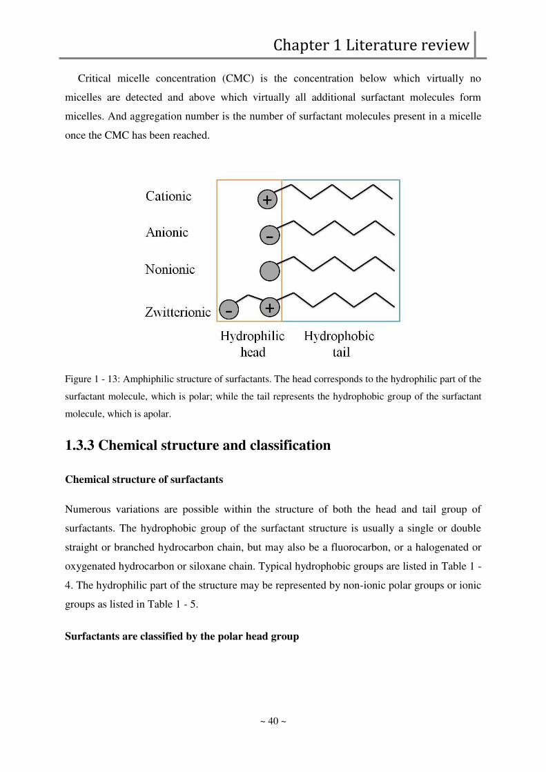
133 Chemical structure and classification 40
134 Properties of surfactants 43
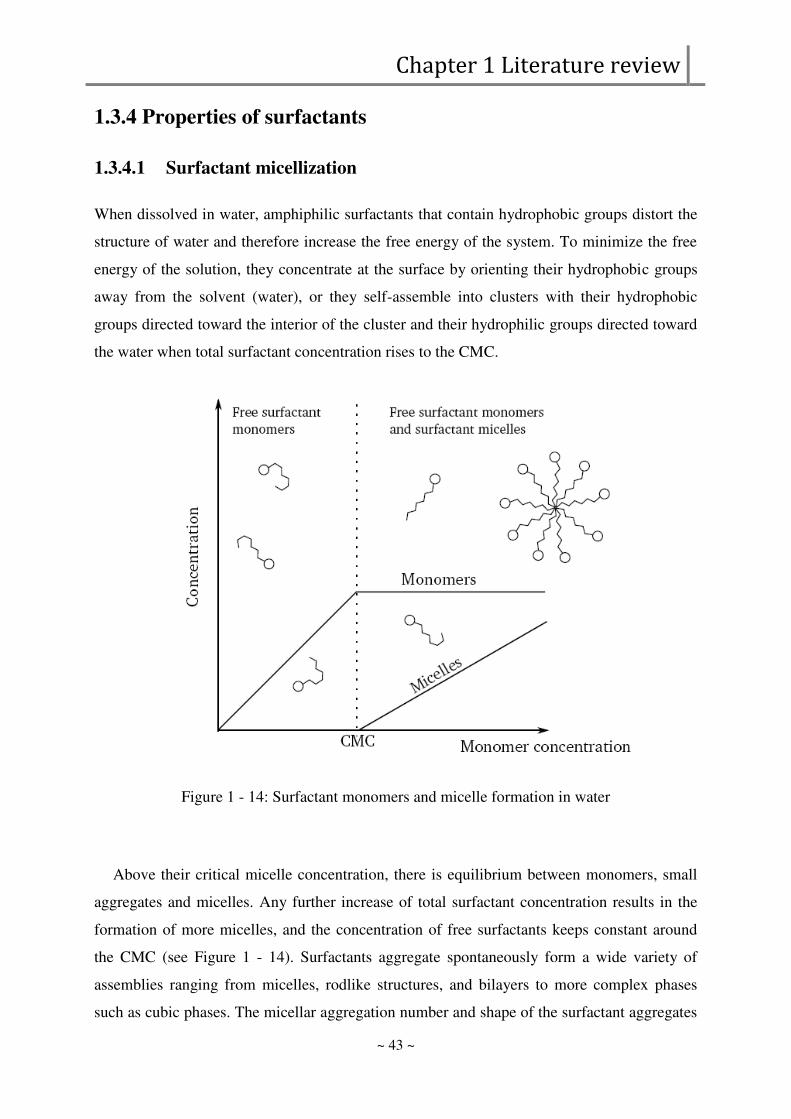
1341 Surfactant micellization 43
1342 Surfactant adsorption at solid-liquid interface 44
135 Environmental effects of surfactant 51
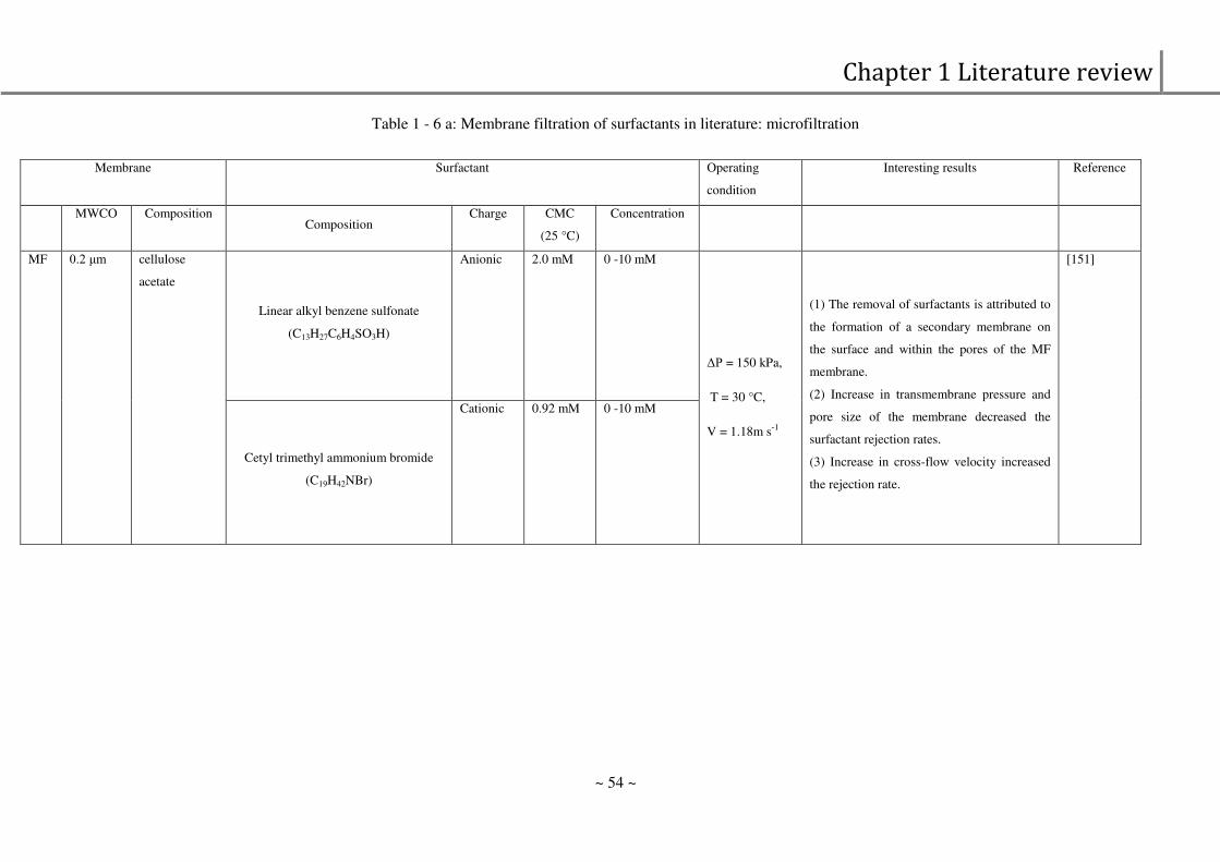
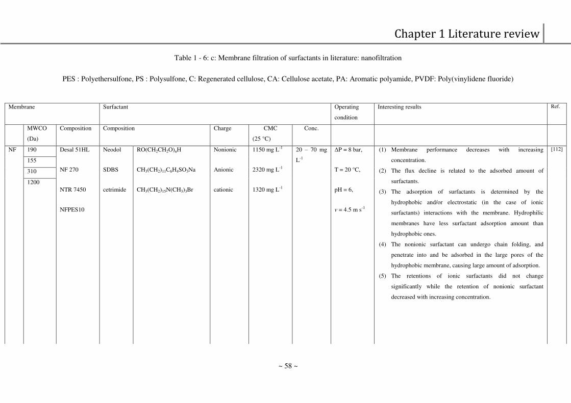
136 Membrane filtration of surfactants 52
14 Membrane filtration 62
15 Simulation of surfactant systems 63
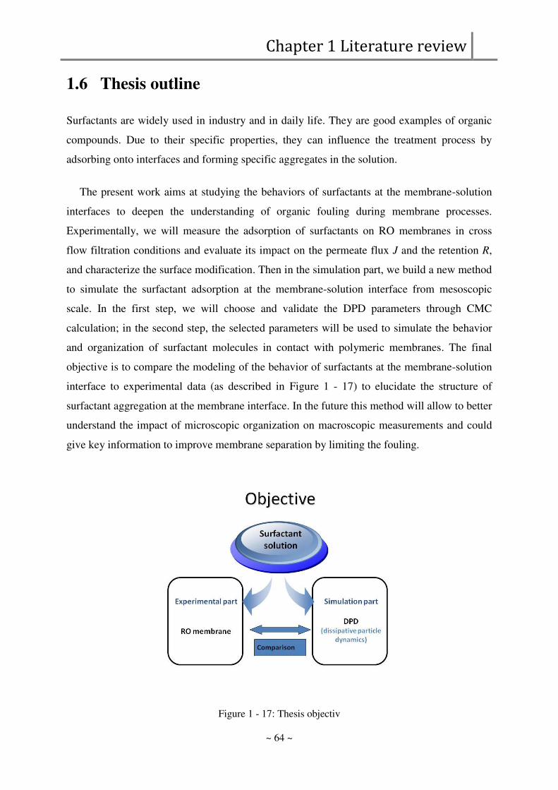
16 Thesis outline 64
Chapter 2 65
Experimental part 65
Fouling of RO membranes by surfactants 65
21 Introduction 67
22 Materials and methods 69
221 Surfactant solutions 69
222 RO membranes 69
223 Analytical methods 71
224 Filtration set-up and reverse osmosis of surfactant solutions 71
225 Adsorption in reverse osmosis set-up without pressure 74
226 Static adsorption of surfactants onto SG membranes 74
227 Contact angle measurements 75
23 Results 77
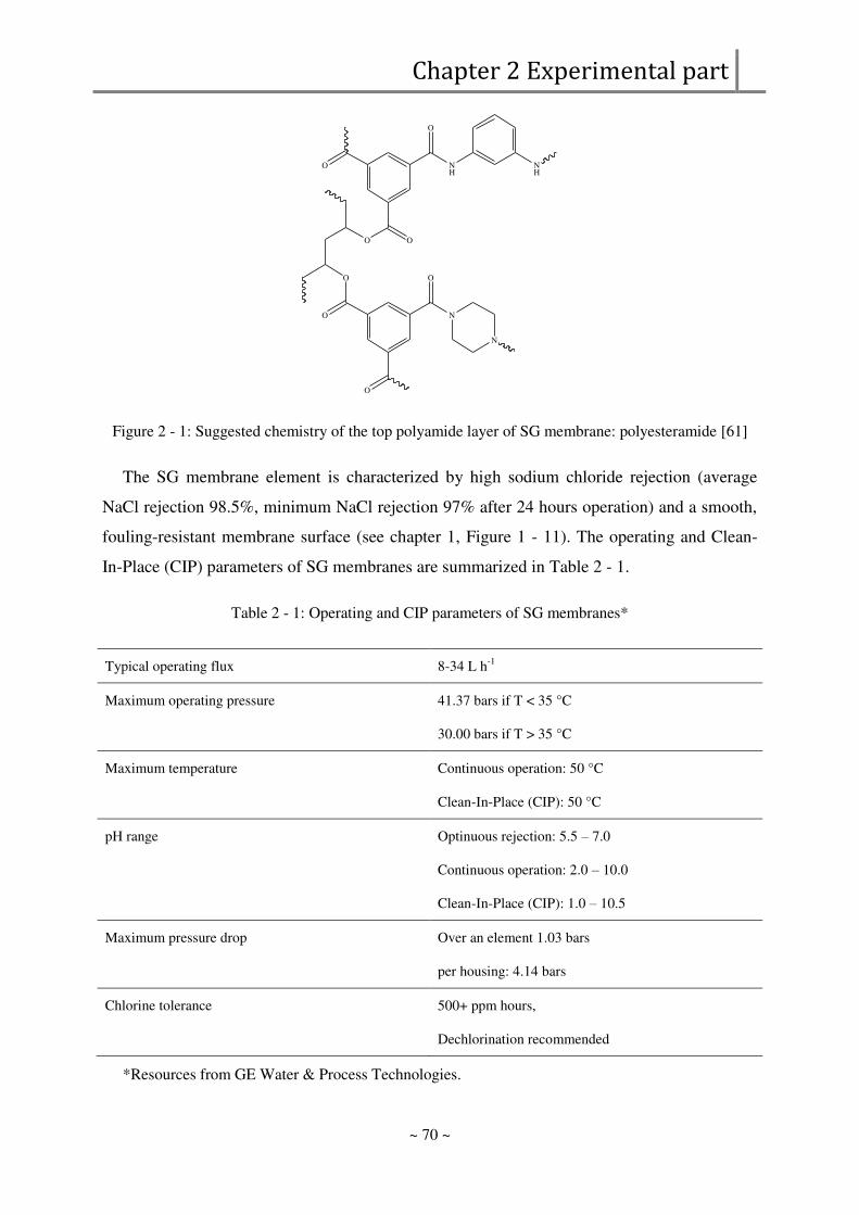
231 Membrane performance 77
2311 SDS rejection 77
2312 Permeate flux 79
232 Surfactant adsorption 83
~ v ~
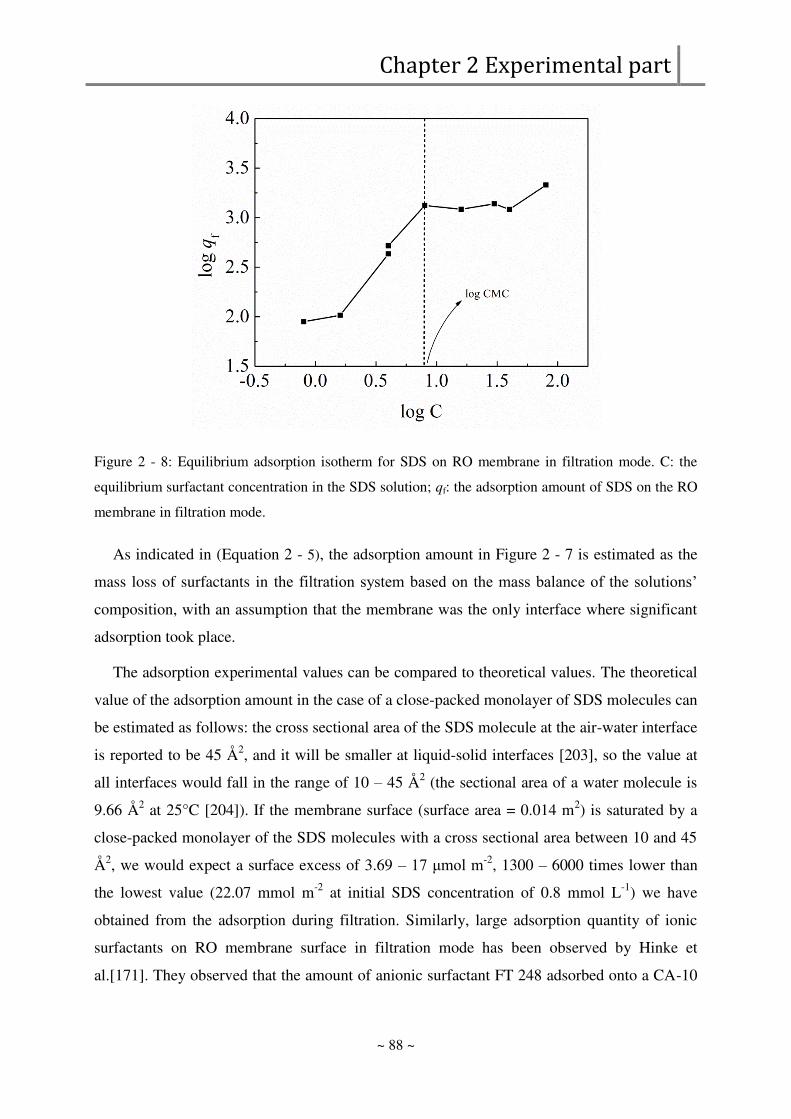
2321 Adsorption during filtration process 83
2322 Adsorption in the filtration system 89
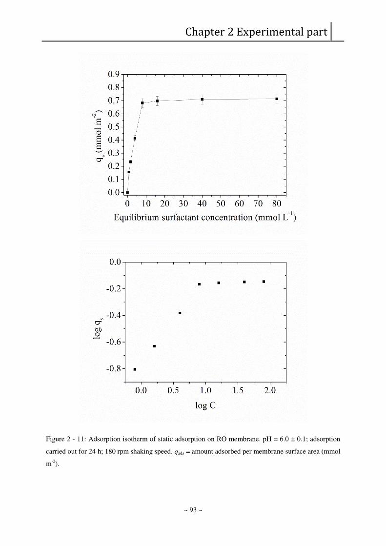
2323 Static adsorption 91
2324 Circulation of surfactant solution in the system without pressure 95
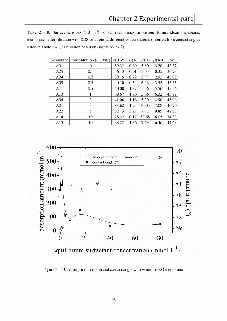
233 Contact angle measurements 97
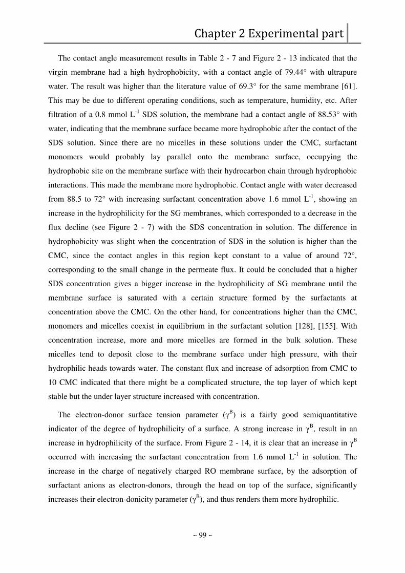
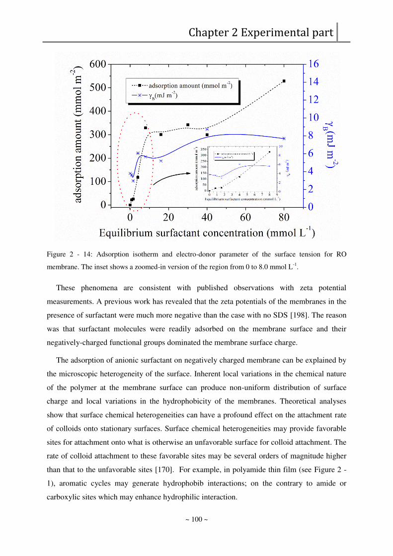
234 Mechanism of surfactant adsorption onto membrane surface 101
24 Conclusions 105
Chapter 3 107
Simulation part 107
Mesoscopic simulations 107
of surfactant micellization and adsorption 107
by Dissipative Particle Dynamics 107
31 Introduction 109
32 Theory 113
Dissipative Particle Dynamics 113
33 Methodology 117
331 DPD Models for surfactants and water 117
332 Detailed DPD simulation procedure 118
333 Analysis details 121
3331 Micelle formation 121
3332 Cluster definition 124
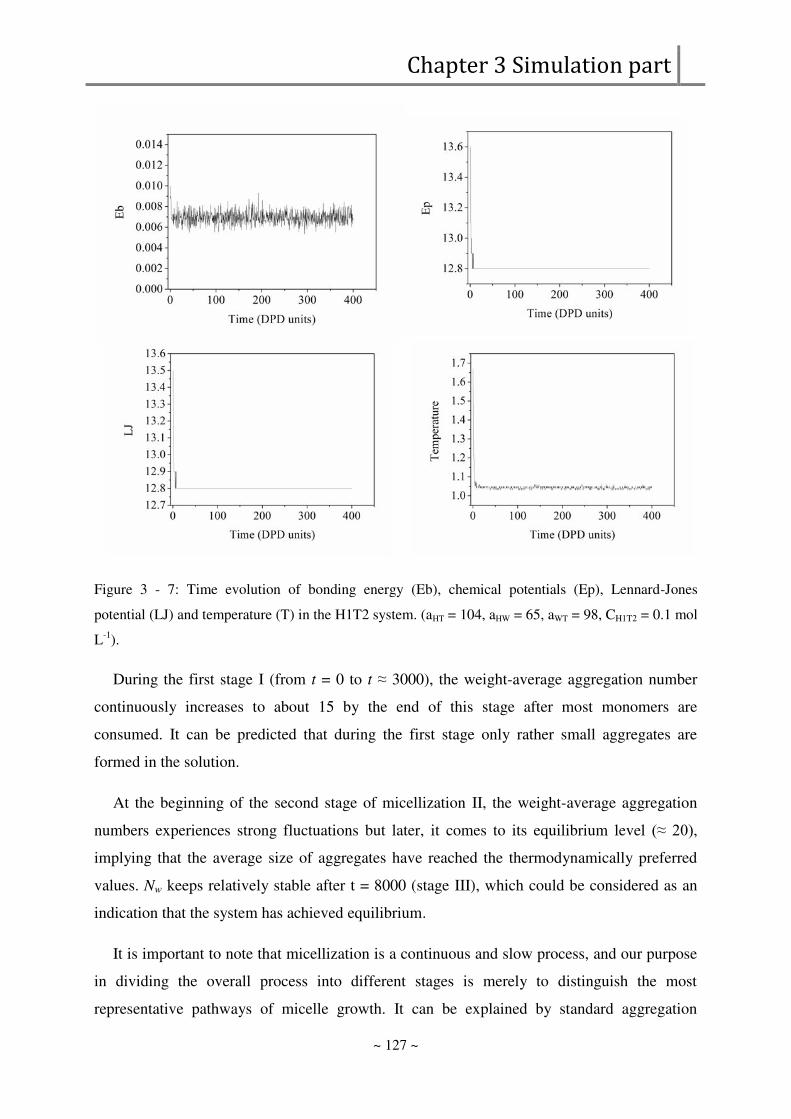
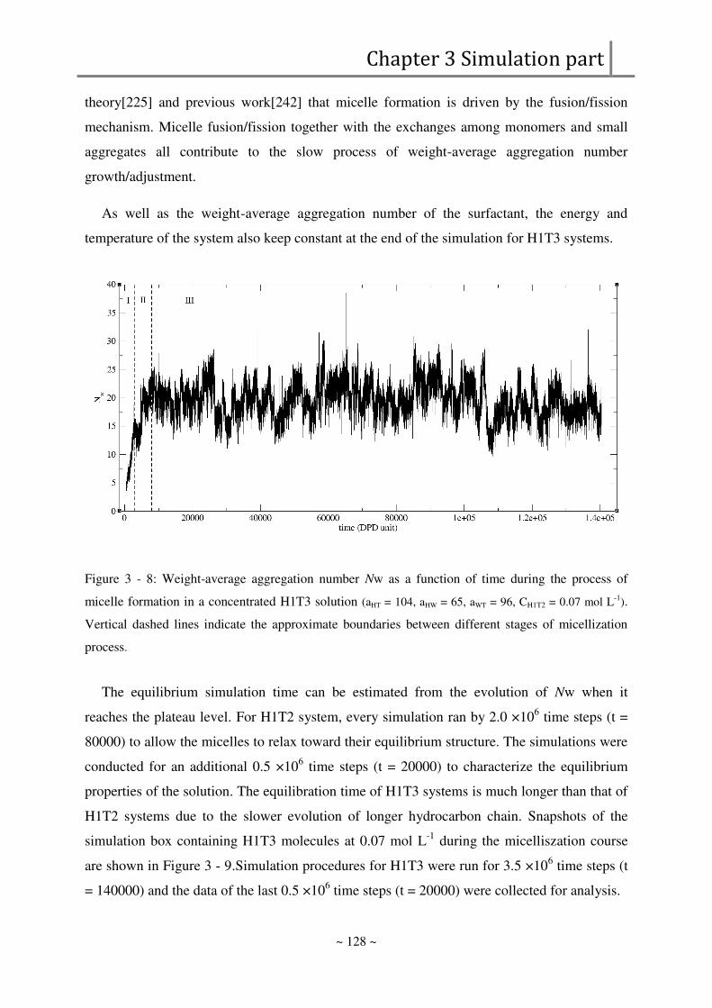
3333 Equilibrium 126
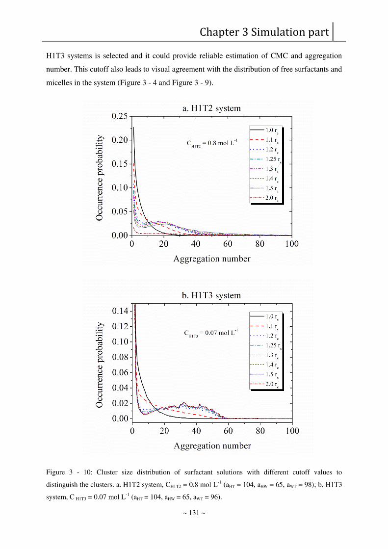
3334 Cluster size distribution 130
3335 Critical micelle concentration 134
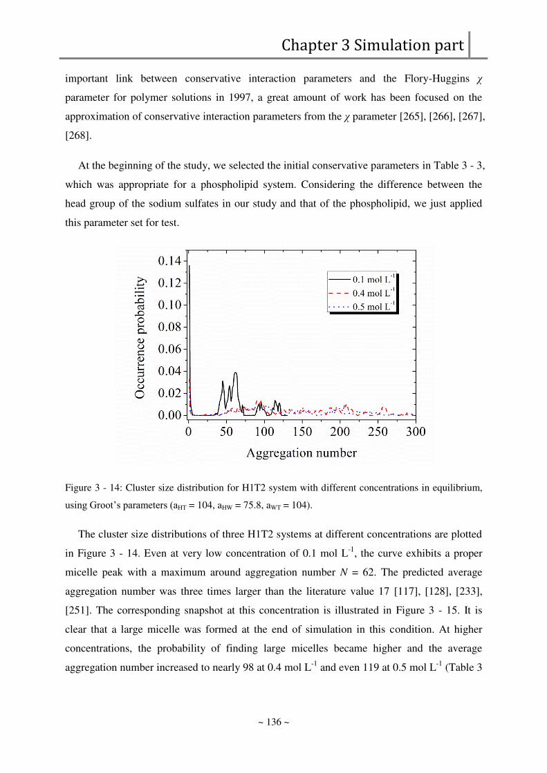
34 Results and discussion 135
341 Parameter set I 135
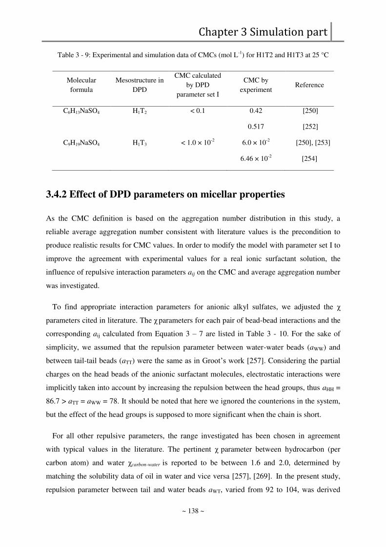
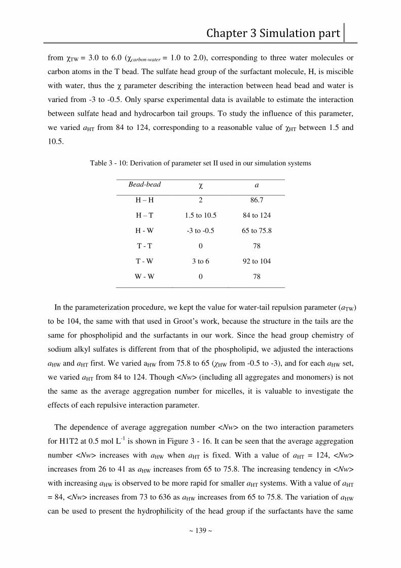
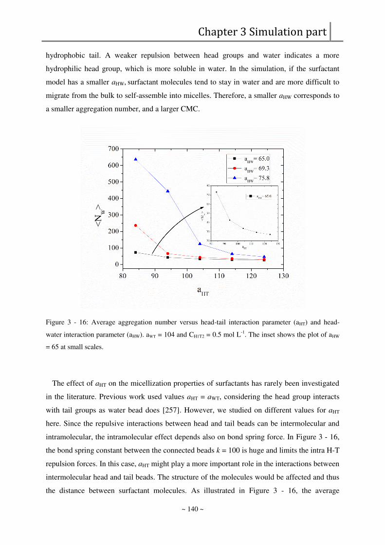
342 Effect of DPD parameters on micellar properties 138
~ vi ~
343 Effect of intramolecular interactions 142
344 CMC of surfactants 147
345 Adsorption of surfactants on the membrane 151
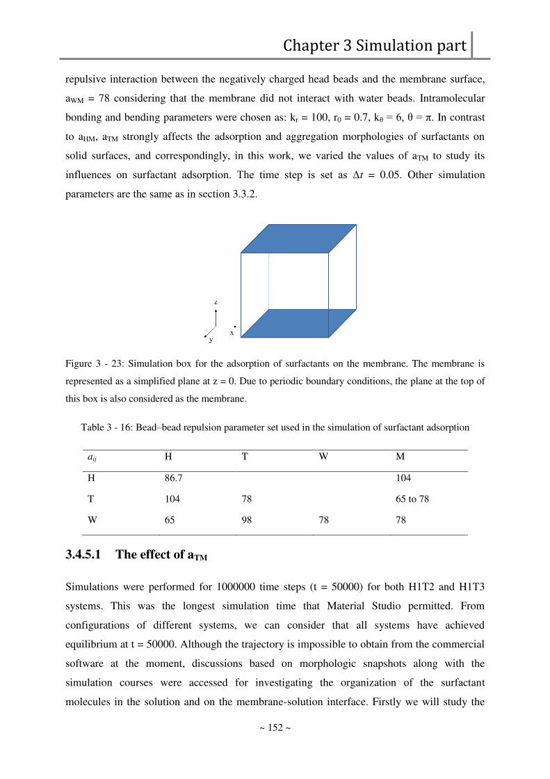
3451 The effect of aTM 152
3452 The effect of surfactant concentration 154
3453 Kinetic competition between micellization and adsorption 157
35 Conclusion 159
General conclusions and perspectives 161
Appendix 169
References 173
~ vii ~
Nomenclature
1 Symbols
a0 Cross-sectional area Aring2
aij aii Conservative repulsion parameters in DPD
A Am Membrane surface area m-2
ASDS Cross-sectional area of SDS molecules Aring2
C0 Initial concentration mol L-1
CAm Maximum concentration of solute A at the membrane surface
mol L-1
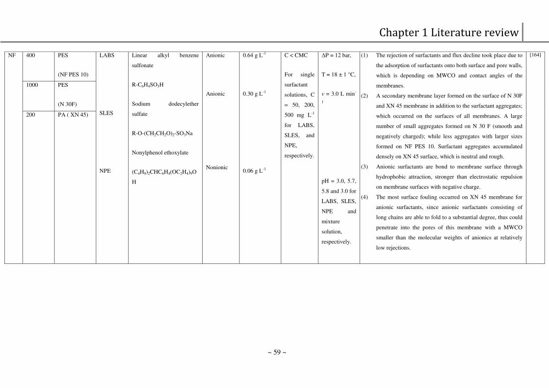
CAf Bulkfeed concentration of solute A mol L-1
CC Concentrate solute concentration mol L-1
Ceq Equilibrium concentration of the surfactant in solution mol L-1
CF Feed solute concentration mol L-1
CP Permeate solute concentration mol L-1
Ct Retentate concentration when samples are taken at each time interval during RO filtration experiments
mol L-1
dp Diameter of membrane pores m
e Membrane thickness m
Eb Bonding energy
Ep Chemical potentials in DPD system
FC Concentrate flow rate L h-1
FF Feed flow rate L h-1
Fi Total force on bead i in DPD simulation
FB Bending force in DPD
Cij F
Dij F
Rij F Conservative force dissipative force and random force in
DPD
FP Permeate flow rate L h-1
Fs Harmonic spring force between bonded beads in DPD simulation
g(r) Radial distribution function
J Flux L h-1 m-2
JS Solute flux L h-1 m-2
~ viii ~
Jw Water flux L h-1 m-2
Jw0 Initial or pure water flux L h-1 m-2
kB Boltzmanns constant
Kf nf Constants for a given adsorbate and adsorbent pair at a particular temperature
KH Henry adsorption constant L m-2
KL Langmuir constant L mol-1
kr Bond spring constant in DPD simulation
kθ Bending constant in DPD simulation
KS Equilibrium constant of the surface aggregation process
lc Length of surfactant hydrophobic group in the core of a micelle
Aring
mout Total mass of SDS taken out as samples during RO filtration experiments
g
MSDS Molar mass of SDS molecules g mol-1
Nagg Aggregation number
ni Number of aggregates in the simulated system
N Cluster size
Ni Number of surfactants that belong to cluster i
Nm Number of water molecules contained in one bead
Nw Weight-average aggregation number
ns Average aggregation number of the surface aggregate as a general adsorption isotherm
pHF Feed pH
Qads Amount of surfactant adsorption onto the adsorbent mol m-2 or g m-2
Qadmax Maximum adsorption of the surfactant per unit mass of the UF membranes
mol m-2
qf Mass loss of surfactant during filtration per membrane surface
mmol m-2
Qinfin The limiting surfactant adsorption at high concentration mmol m-2
qs Amount of surfactant adsorbed onto the membrane in static adsorption experiments
mmol m-2
r Water recovery of the membrane
r0 Equilibrium distance between two consecutive beads in DPD simulation
~ ix ~
rc Cutoff radius in DPD simulation
R Solute rejection
Rcm Distance between surfactant centers of mass
ri Position of a bead in DPD
RADS Resistance for adsorption
Ragg Cutoff threshold to distinguish micelles and free surfactants
RCL Resistance for cake layer
RF Membrane resistance caused by fouling
RG Resistance for gel layer
Rm Membrane resistance
Rt Total resistance of all the individual resistance that may happen for a given solution-membrane system
T Temperature
v Velocity of the flow m s-1
vij equal to vi minus vj the velocity difference between beads i and j in DPD simulation
V Volume L
V0 VHold Vout Initial hold-up and taken out volume of the filtration system
L
VH Volume occupied by surfactant hydrophobic groups in the micellar core
Aring3
W Adhesion between solid and liquid
X1 Xaggi Molar fraction of of the surfactant monomers and the surfactant aggregate with aggregation number i
~ x ~
2 Greek letters
Δa Interfacesurface area m-2
ΔG0 Free energy of adsorption at infinite dilution J
ΔGI Interfacial free energy J
ΔGii Free energy of cohesion i in vacuo J
ΔGsl Free energy of interaction required to separate the surface S and a liquid L
J
σij Fluctuation amplitude in DPD simulation
ε Membrane porosity
Δ Osmotic pressure bar
ΔP Transmembrane pressure bar
Δt Time step in DPD simulation
ζ Zeta potential mV
Interfacialsurface tension J m-2
1 2 i Surface tension of materials 1 2 or i J m-2
AB Lewis acidbase (polar)
A B Electron acceptor and electron donor parameters of the surface tension
lv Liquid-vapor surface tension
sl Solid and liquid interfacial tension
sv Solid-vapor surface tension
LW Lifshitz-Van der Waals component of the surface tension
γij Friction coefficient in DPD simulation
ρ Density of the simulation system
θ Contact angle deg
θ0 Equilibrium angle in DPD simulation
μ1 μagg Chemical potential of free surfactant monomers and aggregates
ωD(rij) ωR(rij) Weight function for dissipative force and random force in DPD simulation
χ FloryndashHuggins parameter
ξij Noise coefficient in DPD simulation
~ xi ~
3 Acronym
AFM Atomic force microscopy
ATR-FTIR Attenuated total Reflectance Fourier transform Infrared Spectroscopy
BOD Biological oxygen demand g O2 L-1
CA Cellulose acetate
CAC Critical aggregation concentration
CESIO Comiteacute Europeacuteen des Agents de Surface et leurs intermeacutediaires Organiques
CG-MD Coarse-grained molecular dynamics
CIP Clean-In-Place
CM Center of mass
CMC Critical micelle concentration
COD Chemical oxygen demand g O2 L-1
CP Concentration polarization
CSLM Confocal scanning laser microscopy
CTAB Hexadecyltrimethylammonium bromide
DPD Dissipative Particle Dynamics
EDS Energy-Dispersive X-ray Spectroscopy
EIS Electrochemical impedance spectroscopy
ELSD Evaporative light scattering detector
ESCA Spectroscopy for chemical analysis
FH Flory-Huggins
HPLC High performance liquid chromatography
IR Infrared Spectroscopy
MD Molecular dynamics simulation
MEUF Micellar-enhanced ultrafiltration
MF Microfiltration
MP Membrane potential
MSD Mean square displacement
MWCO Molecular weight cut-off Da
NF Nanofiltration
~ xii ~
NP Polyoxyethylene nonylphenyl ether
NVT Constant particle number volume and temperature
PA Polyamide
PES Polyethersulfone
PFOS Perfluorooctane sulfonate
PVC Polyvinyl chloride
PVDF Poly(vinylidene fluoride)
RDF Radial distribution function
RO Reverse osmosis
SBE Backscattered electrons
SDBS Sodium dodecyl benzene sulfonate
SDS Sodium dodecyl sulfate
SE Secondary electrons
SEM Scanning electron microscope
SHS Sodium hexyl sulfate C6H13OSO3Na
SIMS Secondary Ion Mass Spectroscopy
SNS Sodium nonyl sulfate C9H19OSO3Na
SP Streaming potential
TDBNC Tetradecylbenzylammonium chloride
TEM Transmission electron microscope
TFC Thin film composite
TMP Transmembrane pressure bar
TOC Total organic carbon g O2 L-1
TOF-SIMS Secondary Ion Mass Spectroscopy combined with a mass analyzer called time-of-flight
UF Ultrafiltration
XPS X-ray Photoelectron Spectroscopy
General introduction
General introduction
~ 2 ~
General introduction
~ 3 ~
Because of vastly expanding populations increasing water demand and the deterioration of
water resource quality and quantity water is going to be one of the most precious resources in
the world The problem of water shortage is not only a problem of proper techniques but also
a social and educational problem depending on national and international efforts as well as on
technical solutions [1]
In water and wastewater treatment membrane technology a term that refers to a number of
different processes using synthetic membranes to separate chemical substances has been
recognized as the key technology for the separation of contaminants from polluted sources
thus purifying original waters [1] Membranes are selective barriers that separate two different
phases allowing the passage of certain components and the retention of others The driving
force for transport in membrane processes can be a gradient of pressure chemical potential
electrical potential or temperature across the membrane Membrane processes rely on a
physical separation usually with no addition of chemicals in the feed stream and no phase
change thus stand out as alternatives to conventional processes (ie distillation precipitation
coagulationflocculation adsorption by active carbon ion exchange biological treatmenthellip)
for the chemical pharmaceutical biotechnological and food industries [1] [2] In many cases
the low energy consumption reduction in number of processing steps greater separation
efficiency and improved final product quality are the main attractions of these processes [1]
[2] [3] During the past years membranes have been greatly improved with significantly
enhanced performance and commercial markets have been spreading very rapidly throughout
the world In the future further improvements and innovations are needed especially in the
chemical and morphological design of membrane materials element and module design of
membrane systems antifouling membranes for wastewater treatment and so on [1]
Among all technologies available today reverse osmosis (RO) is gaining worldwide
acceptance in both water treatment and desalination applications [4] RO membranes can be
used to remove salinity and dissolved organic matter while reducing total organic carbon
(TOC) chemical oxygen demand (COD) and biological oxygen demand (BOD) [1] The mass
transfer in RO is due to solution-diffusion mechanism size exclusion charge exclusion and
physical-chemical interactions between solute solvent and the membrane [4] The process
efficiency is determined by several factors including operational parameters membrane and
feed water properties The most common commercially available RO membrane modules
include flat sheet and spiral-wound RO membranes with integrally asymmetric structure from
the first generation material cellulose acetate (CA) to thin film composite (TFC) membranes
General introduction
~ 4 ~
are most available in the market Most of commercial RO composite membranes are
polyamide-based while other composite membranes (ie sulfonated polysulfone) could also
be found [2]The functional groups introduced into the polymer structure control the valence
and strength of the membrane charge while the degree of adsorption of dissolved species is
determined by membrane hydrophobicity charge and roughness affect [4] [5]
Though the improvement of RO membranes has been tremendous in the past few years
their performance and economics are still far from perfect Membrane life time and permeate
fluxes are primarily affected by the phenomena of concentration polarization and fouling [6]
During the pressure-driven membrane processes of aqueous effluent containing dissolved
organic matters membrane fouling leads to a decrease in performance with a loss in solvent
permeability and changes to solute transmission The reasons for fouling are reported as
consisting of chemical fouling biological fouling and scale formation [1] Organic fouling is
caused by the adsorption of organic materials from the feed water such as humic substances
proteins polysaccharides surfactants etc onto or into the membrane [2] The chemical
fouling depends on hydrophobic interaction and electrostatic interaction between organic
materials in the feed water and membrane surface [7]
In this study we focus on membrane fouling by surfactants Surfactants are organic
compounds used in everyday life and are essential components in many industrial processes
and formulations such as household detergents personal care formulations industrial and
institutional washing and cleaning as well as numerous technical applications such as textile
auxiliaries leather chemicals agrochemicals (pesticide formulations) metal and mining
industry plastic industry lubricants paints polymers pharmaceutical oil recovery pulp and
paper industry etc [8] They are also occasionally used for environmental protection eg in
oil slick dispersions [9] Moreover surfactants are molecules with a relatively simple
structure compared to proteins for example and constitute a good example of amphiphilic
organic matter
Surfactants have both hydrophobic (the ldquotailrdquo) and hydrophilic (the ldquoheadrdquo) groups they
can easily self-assemble into the ordered structures at mesoscopic scale (such as micelles
layers and liquid crystals etc) They can also interact in different ways with the membranes
The adsorption of surfactants on membrane surfaces in the form of monomers or surface
aggregates affect mass transfer and surface characteristics of the membranes thus the
performance and efficiency of the membrane filtration
General introduction
~ 5 ~
Although RO membranes have received much attention from both academy and industry
and many methods have been proposed to characterize RO membranes in order to obtain
structural parameters the fouling mechanisms of solutes (especially organic components) on
the membranes are still not fully understood Relevant experimental methods permit to
identify the mass and sometimes the nature of organic fouling as well as the change in the
surface tension Though they can localize large structure of accumulated matter the
organization of the compounds at the surface and the nature of interaction with the polymer is
still not accessible at the moment The physical and chemical phenomena involved in the
fouling process on dense membranes like those used in RO require building relevant modeling
tools to show how molecular interactions are manifested in the microscopic domain as well as
how microscopic phenomena are manifested in the macroscopic world that we perceive from
experiments [10]
The reproduction or prediction of properties for a preselected system usually requires an
accurate model The most accurate method to simulate the hydrodynamic comportment of an
atomistic system is to integrate the equations of motion for all atoms in the system This is the
basis of the molecular dynamics (MD) simulation methods The MD reproduces every aspect
of the atomic motion which is often too detailed to allow an understanding of physical
processes and is limited to a few thousand molecules over a few nanoseconds because of
computer processor speeds and memory capacities If the hydrodynamic collective behavior
occurred for time much longer than the collision time and for distance much larger than inter
particle distance this approach is inadequate In the same way macroscopic simulation starts
at a length scale where the materials are sufficiently homogeneous to justify a continuum
description In the membrane processes studies macroscopic simulation is able to describe
flux through membrane versus global resistances diffusion coefficient and mean
concentrations at the interfaces but it does not allow understanding the specific organization
of organic molecules in the bulk in the concentration polarization layer nor in the membrane
Many phenomena occur at mesoscopic scales such as surfactant-polymer interaction
Dissipative particle dynamics (DPD) is an intermediate simulation method allowing the
investigation of mesoscopic systems containing millions of atoms with length scale between
10-6 and 10-3 m and time scale between 10-6 and 10-3 s respectively [11] [12] However the
DPD models for adsorption onto RO membranes are not found in literature
The objective of this thesis is to deepen the understanding of fouling by modeling the
behavior of organic molecules at the membrane interface and by comparing these simulation
General introduction
~ 6 ~
results to experimental data A previous thesis work on RO process of mixed surfactant
solutions showed a high rejection of surfactants with a thin-film composite membrane but the
membrane fouling caused by anionic surfactant adsorption during RO processes is significant
[13]
The manuscript is outlined as follows In the first chapter we briefly recall the necessary
definitions on pressure-driven membrane processes paying special attention to RO processes
and then provide an overview of surfactants The second chapter is devoted to the
experimental study of surfactant adsorption on reverse osmosis membrane The evolution of
RO process performances (flux retention rate) and the surface properties of the membrane
surface are investigated The third chapter deals with DPD simulations of anionic surfactants
in aqueous solutions and at the membrane interface The micellization properties in
equilibrium (eg the critical micelle concentration and aggregation number) of surfactants are
inferred from the mesoscopic simulations and compared with bulk solution properties from
experiments Investigation on surfactants organization at the membrane interface during
reverse osmosis filtration was undertaken by adding a simplified membrane surface to the
surfactant system The interactions between membrane and surfactants are investigated
Chapter 1
Literature review
Chapter 1 Literature review
~ 8 ~
Chapter 1 Literature review
~ 9 ~
The aim of this work is to get a better understanding of the microscopic behavior of organic
matters during the membrane processes for the treatment of complex mixtures This chapter
provides a research-based overview of the background information on the membrane
processes the target composition we are going to treat with and the available technologies in
literature to investigate the phenomena that might occur during the membrane processes
This bibliographic chapter is divided into five parts
- The first part presents different membrane processes and their applications
- The second part presents different methods to investigate the physical-chemical
characteristics of the membranes
- The third part presents the surfactants
- The fourth part presents the state-of-art on the simulation methods
- The last part presents the problematic and objective of this thesis
11 Pressure-driven membrane processes
111 Definition
Membrane technology covers a number of different processes for the transport of substances
between two fractions with the help of permeable membranes [14] Membranes used in
membrane technology may be regarded as selective barriers separating two fluids and
allowing the passage of certain components and the retention of others from a given mixture
implying the concentration of one or more components The driving force for the transport is
generally a gradient of some potential such as pressure temperature concentration or electric
potential [14]
One of the particular advantages of membrane separation process is that it relies on a
physical separation usually with no addition of chemicals in the feed stream and without
phase change [15] Moreover it can be operated without heating Therefore this separation
process is energetically usually lower than conventional separation technologies (ie
distillation crystallization adsorption) Whatrsquos more it responds more efficiently to the
requirements of process intensification strategy because it permits drastic improvements in
industrial production substantially decreasing the equipment-sizeproduction-capacity ratio
Chapter 1 Literature review
~ 10 ~
energy consumption andor waste production so resulting in sustainable technical solutions
[16] Although typically thought to be expensive and relatively experimental membrane
technology is advancing quickly becoming less expensive improving performance and
extending life expectancy It has led to significant innovations in both processes and products
in various industrial sectors (eg chemical pharmaceutical biotechnological food sectors etc)
over the past few decades
112 Membrane flow configurations
Membrane systems can be operated in various process configurations There are two main
flow configurations of membrane processes dead-end and crossflow filtrations as presented
in Figure 1 - 1 In a conventional filtration system the fluid flow be it liquid or gaseous is
perpendicular to the membrane surface In this dead-end filtration there is no recirculation of
the concentrate thus solutes are more probable to deposit on the membrane surface and the
system operation is based on 100 recovery of the feed water In crossflow filtration the feed
flow is tangential to the membrane surface and then divided into two streams The retentate or
concentrate (solution that does not permeate through the surface of the membrane) is re-
circulated and blended with the feed water whereas the permeate flow is tracked on the other
side [1] [17]
Both flow configurations offer some advantages and disadvantages The dead-end
membranes are relatively less costly to fabricate and the process is easy to implement The
main disadvantage of a dead-end filtration is the extensive membrane fouling and
concentration polarization which requires periodic interruption of the process to clean or
substitute the filter [3] The tangential flow devices are less susceptible to fouling due to the
sweeping effects and high shear rates of the passing flow
Chapter 1 Literature review
~ 11 ~
Figure 1 - 1 Membrane flow configurations Left Crossflow filtration Right Dead-end filtration
(Source wwwspectrumlabscomfiltrationEdgehtml)
113 Types of membranes MF UF NF RO
Membrane separation processes have very important role in separation industry The first
industrial applications of pressure driven membrane processes were water desalination by
reverse osmosis in 1960rsquos [1] There are basically four pressure driven membrane processes
allowing separation in the liquid phase microfiltration (MF) ultrafiltration (UF)
nanofiltration (NF) and reverse osmosis (RO) These processes are distinguished by the
application of hydraulic pressure as the driving force for mass transport Nevertheless the
nature of the membrane controls which components will permeate and which will be retained
since they are selectively separated according to their molar masses particle size chemical
affinity interaction with the membrane [3]
The pore size of a membrane is generally indicated indirectly by membrane manufacturers
through its molecular weight cut-off (MWCO) which is usually expressed in Dalton (1 Da =
1g mol-1) [3] MWCO is typically defined as the molecular weight of the smallest component
that will be retained with an efficiency of at least 90
Chapter 1 Literature review
~ 12 ~
Figure 1 - 2 Cut-offs of different liquid filtration techniques [18]
Figure 1 - 2 relates the size of some typical particles both to the pore size and the
molecular weight cut off of the membranes required to remove them The separation spectrum
for membranes as illustrated in Figure 1 - 2 [19] ranges from reverse osmosis (RO) and
nanofiltration (NF) for the removal of solutes to ultrafiltration (UF) and microfiltration (MF)
for the removal of fine particles Table 1 - 1 shows size of materials retained driving force
and type of membrane for various membrane separation processes
Table 1 - 1 Size of Materials Retained Driving Force and Type of Membrane [1]
Process Minimum particle size removed
Applied pressure Type of membrane
Microfiltration 0025 - 10 microm microparticles
(01 - 5 bar)
Porous
Ultrafiltration 5 - 100 nm macromolecules
(05 - 9 bar)
Porous
Nanofiltration 05 - 5 nm molecules
(4 - 20 bar) Porous
Reverse Osmosis lt 1 nm salts
(20 - 80 bar) Nonporous
Chapter 1 Literature review
~ 13 ~
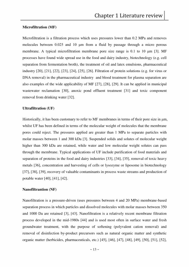
Microfiltration (MF)
Microfiltration is a filtration process which uses pressures lower than 02 MPa and removes
molecules between 00β5 and 10 μm from a fluid by passage through a micro porous
membrane A typical microfiltration membrane pore size range is 01 to 10 μm [3] MF
processes have found wide spread use in the food and dairy industry biotechnology (eg cell
separation from fermentation broth) the treatment of oil and latex emulsions pharmaceutical
industry [20] [21] [22] [23] [24] [25] [26] Filtration of protein solutions (eg for virus or
DNA removal) in the pharmaceutical industry and blood treatment for plasma separation are
also examples of the wide applicability of MF [27] [28] [29] It can be applied in municipal
wastewater reclamation [30] anoxic pond effluent treatment [31] and toxic component
removal from drinking water [32]
Ultrafiltration (UF)
Historically it has been customary to refer to MF membranes in terms of their pore size in μm
whilst UF has been defined in terms of the molecular weight of molecules that the membrane
pores could reject The pressures applied are greater than 1 MPa to separate particles with
molar masses between 1 and 300 kDa [3] Suspended solids and solutes of molecular weight
higher than 300 kDa are retained while water and low molecular weight solutes can pass
through the membrane Typical applications of UF include purification of food materials and
separation of proteins in the food and dairy industries [33] [34] [35] removal of toxic heavy
metals [36] concentration and harvesting of cells or lysozyme or liposome in biotechnology
[37] [38] [39] recovery of valuable contaminants in process waste streams and production of
potable water [40] [41] [42]
Nanofiltrantion (NF)
Nanofiltration is a pressure-driven (uses pressures between 4 and 20 MPa) membrane-based
separation process in which particles and dissolved molecules with molar masses between 350
and 1000 Da are retained [3] [43] Nanofiltration is a relatively recent membrane filtration
process developed in the mid-1980s [44] and is used most often in surface water and fresh
groundwater treatment with the purpose of softening (polyvalent cation removal) and
removal of disinfection by-product precursors such as natural organic matter and synthetic
organic matter (herbicides pharmaceuticals etc) [45] [46] [47] [48] [49] [50] [51] [52]
Chapter 1 Literature review
~ 14 ~
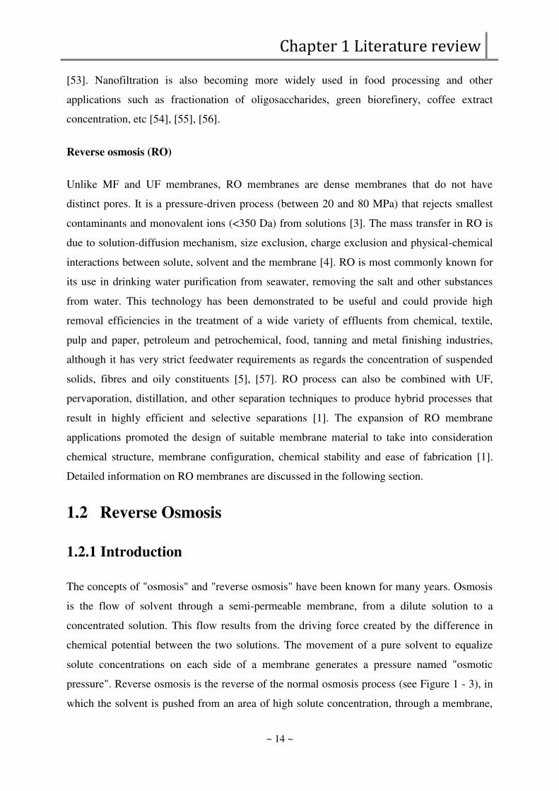
[53] Nanofiltration is also becoming more widely used in food processing and other
applications such as fractionation of oligosaccharides green biorefinery coffee extract
concentration etc [54] [55] [56]
Reverse osmosis (RO)
Unlike MF and UF membranes RO membranes are dense membranes that do not have
distinct pores It is a pressure-driven process (between 20 and 80 MPa) that rejects smallest
contaminants and monovalent ions (lt350 Da) from solutions [3] The mass transfer in RO is
due to solution-diffusion mechanism size exclusion charge exclusion and physical-chemical
interactions between solute solvent and the membrane [4] RO is most commonly known for
its use in drinking water purification from seawater removing the salt and other substances
from water This technology has been demonstrated to be useful and could provide high
removal efficiencies in the treatment of a wide variety of effluents from chemical textile
pulp and paper petroleum and petrochemical food tanning and metal finishing industries
although it has very strict feedwater requirements as regards the concentration of suspended
solids fibres and oily constituents [5] [57] RO process can also be combined with UF
pervaporation distillation and other separation techniques to produce hybrid processes that
result in highly efficient and selective separations [1] The expansion of RO membrane
applications promoted the design of suitable membrane material to take into consideration
chemical structure membrane configuration chemical stability and ease of fabrication [1]
Detailed information on RO membranes are discussed in the following section
12 Reverse Osmosis
121 Introduction
The concepts of osmosis and reverse osmosis have been known for many years Osmosis
is the flow of solvent through a semi-permeable membrane from a dilute solution to a
concentrated solution This flow results from the driving force created by the difference in
chemical potential between the two solutions The movement of a pure solvent to equalize
solute concentrations on each side of a membrane generates a pressure named osmotic
pressure Reverse osmosis is the reverse of the normal osmosis process (see Figure 1 - 3) in
which the solvent is pushed from an area of high solute concentration through a membrane
Chapter 1 Literature review
~ 15 ~
to an area of low solute concentration Figure 1 - 3 illustrates the processes of osmosis and
reverse osmosis [58] [59]
Figure 1 - 3 Osmosis and reverse osmosis system
(Source httpwwwwqaorg)
Although the concept of RO has been known for many years only since the early 1960rsquos
when an asymmetric cellulose acetate membrane with relatively high water flux and
separation was produced [60] RO process has become both possible and practical on an
industrial scale [44] [60] Since then the development of new-generation membranes such as
the thin-film composite membrane that can tolerate wide pH ranges higher temperatures and
harsh chemical environments and that have highly improved water flux and solute separation
characteristics has resulted in many RO applications It has developed over the past 50 years
to a 44 share in world desalination capacity in 2009 and an 80 share in the total number
of desalination plants installed worldwide [44] In addition to the traditional seawater and
brackish water desalination processes RO membranes have found uses in wastewater
treatment production of ultrapure water water softening and food processing as well as
many others
Chapter 1 Literature review
~ 16 ~
Figure 1 - 4 Schematic of (a) RO Membrane Process and (b) RO Process Streams
122 RO Process description and terminology
A schematic of the RO process is shown in Figure 1 - 4 (a) The RO process consists of a feed
water source a feed pretreatment a high pressure pump RO membrane modules and in
some cases post-treatment steps
The three streams (and associated variables eg FF FC FP CF CC CPhellip) of the RO
membrane process are shown in Figure 1 - 4 (b) the feed the permeate and the concentrate
(or retentate) The water flow through the membrane is reported in terms of water flux Jw
where (Equation 1 - 1)
Chapter 1 Literature review
~ 17 ~
Solute passage is defined in terms of solute flux Js (Equation 1 - 2)
Solute separation is measured in terms of rejection R defined as
(Equation 1 - 3)
The quantity of feed water that passes through the membrane (the permeate) is measured in
terms of water recovery r defined for a batch RO system as
(Equation 1 - 4)
For a continuous system where the flow of each stream is supposed to keep constant the
recovery is defined as (Equation 1 - 5)
In a batch membrane system water is recovered from the system as the concentrate is
recycled to the feed tank as a result if the solute is rejected the feed concentration (CF)
continuously increases over time For a continuous membrane system fresh feed is
continuously supplied to the membrane
Water flux is sometimes normalized relative to the initial or pure water flux (Jwo) as
and flux decline is defined by
(Equation 1 - 6)
Chapter 1 Literature review
~ 18 ~
123 Material structure and geometry
1231 Materials
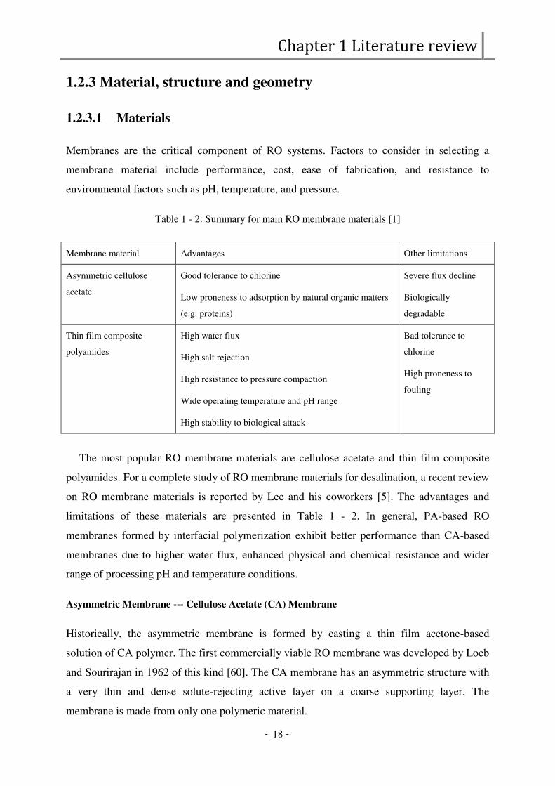
Membranes are the critical component of RO systems Factors to consider in selecting a
membrane material include performance cost ease of fabrication and resistance to
environmental factors such as pH temperature and pressure
Table 1 - 2 Summary for main RO membrane materials [1]
Membrane material Advantages Other limitations
Asymmetric cellulose
acetate
Good tolerance to chlorine
Low proneness to adsorption by natural organic matters
(eg proteins)
Severe flux decline
Biologically
degradable
Thin film composite
polyamides
High water flux
High salt rejection
High resistance to pressure compaction
Wide operating temperature and pH range
High stability to biological attack
Bad tolerance to
chlorine
High proneness to
fouling
The most popular RO membrane materials are cellulose acetate and thin film composite
polyamides For a complete study of RO membrane materials for desalination a recent review
on RO membrane materials is reported by Lee and his coworkers [5] The advantages and
limitations of these materials are presented in Table 1 - 2 In general PA-based RO
membranes formed by interfacial polymerization exhibit better performance than CA-based
membranes due to higher water flux enhanced physical and chemical resistance and wider
range of processing pH and temperature conditions
Asymmetric Membrane --- Cellulose Acetate (CA) Membrane
Historically the asymmetric membrane is formed by casting a thin film acetone-based
solution of CA polymer The first commercially viable RO membrane was developed by Loeb
and Sourirajan in 1962 of this kind [60] The CA membrane has an asymmetric structure with
a very thin and dense solute-rejecting active layer on a coarse supporting layer The
membrane is made from only one polymeric material
Chapter 1 Literature review
~ 19 ~
Thin Film Composite Membrane --- Polyamide (PA) Membrane
The current RO membrane market is dominated by thin film composite (TFC) polyamide
membranes consisting of three layers (see Figure 1 - 5) an ultra-thin selective layer on the
upper surface (0β μm) a microporous interlayer (about 40 μm) and a polyester web acting as
structural support (120ndash150 μm thick) [5] [61]
Figure 1 - 5 Cross-section images of a RO membrane the left image for the whole cross-section ( times
850 magnification) the right image for top cross-section ( times 75000 magnification) [61]
The selective barrier layer is most often made of aromatic polyamide by interfacial
polymerization based on a polycondensation reaction between two monomers a
polyfunctional amine and a polyfunctional acid chloride Some commonly used reactants of
the polyamide thin films are described by Akin and Temelli (see Figure 1 - 6) [61] The
thickness and membrane pore size (normally less than 06 nm) of the barrier layer is reduced
to minimize resistance to the permeate transport and to achieve salt rejection consistently
higher than 99 Therefore between the barrier layer and the support layer a micro-porous
interlayer of polysulfonic polymer is added to enable the ultra-thin barrier layer to withstand
high pressure compression With improved chemical resistance and structural robustness it
offers reasonable tolerance to impurities enhanced durability and easy cleaning
characteristics
Chapter 1 Literature review
~ 20 ~
Figure 1 - 6 The polymerization reactions of most commonly used aromatic PA membranes [61]
1232 Structure
There are mainly two structures for RO membranes asymmetric membranes and composite
membranes Asymmetric membranes are made of a single material (eg CA) with different
structures at different layers only the thin active layer has fine pores that determine the cut-
off while the support layer has larger pores The composite membranes are formed of an
assembly of several layers of material the fine filter layer based on layers of greater porosity
1233 Geometry
Chapter 1 Literature review
~ 21 ~
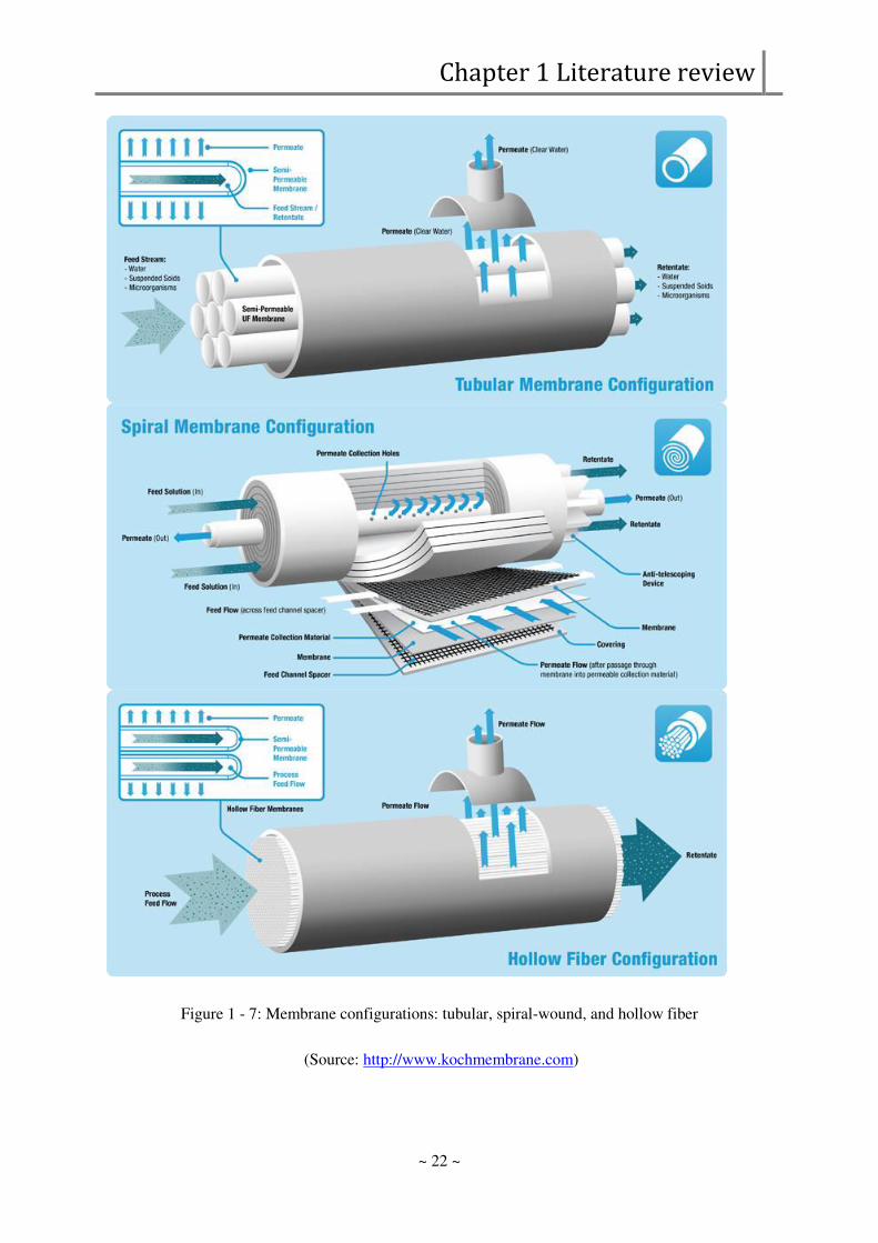
The most common commercially available membrane modules include flat sheet tubular
spiral-wound and hollow fiber elements (see Figure 1 - 7)
Flat sheet membranes are used for the plane modules or in the spiral-wound modules The
tubular modules consist of tube bundles with an inside diameter of 4 to 25 mm This type of
membrane geometry is predominantly used for mineral membranes The hollow fiber
membranes are assembled into the module parallel This kind of membrane is very thin with a
diameter less than 1 mm
The most extensively used design in RO desalination is the spiral wound membrane
module This configuration stands out for high specific membrane surface area easy scale up
operation inter-changeability and low replacement costs and least expensive to produce from
flat sheet TFC membranes [5] Polyamide spiral wound membranes dominate RO NF market
sales with a 91 share Asymmetric cellulose acetate hollow fibre membranes hold a distant
second spot [5]
Chapter 1 Literature review
~ 22 ~
Figure 1 - 7 Membrane configurations tubular spiral-wound and hollow fiber
(Source httpwwwkochmembranecom)
Chapter 1 Literature review
~ 23 ~
124 Concentration polarization and fouling
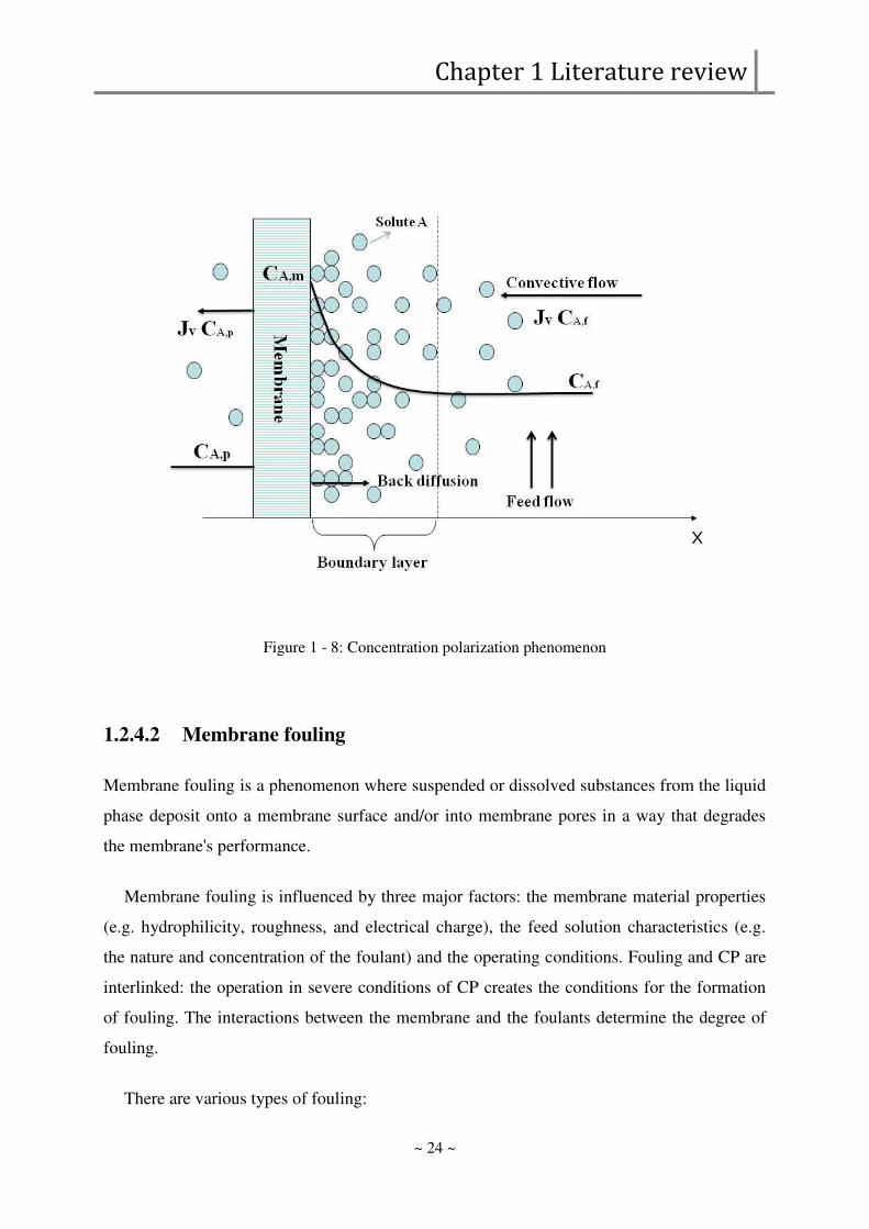
1241 Concentration polarization
The pressure driven fluid flow through a selective membrane convectively transports solute
towards the membrane surface The partially or totally retained solutes will accumulate in a
thin layer adjacent to the membrane surface generating a concentration gradient that is to say
the solute concentration near the membrane surface is much higher than that of the bulk feed
solution As a consequence a diffusive flux of solute back to the feed bulk appears The
solute builds up at the membrane surface until the equilibrium between diffusive and
convective solute fluxes is attained [15] [62] As a result the solute concentration changes
from a maximum at the membrane surface (CAm) to the bulk (CAf) as illustrated in Figure 1 -
8 This phenomenon known as concentration polarization (CP) increases resistance to
solvent flow and thus is responsible for the water flux decline observed in many membrane
filtration processes [63] [64] [65] [66] It is strongly related with the osmotic pressure raise
increase of resistance to permeation (eg gel formation) and fouling susceptibility [62] It
might also change the membrane separation properties for instance due to surface charge
variations The extent of concentration polarization can be reduced by promoting good mixing
of the bulk feed solution with the solution near the membrane surface Mixing can be
enhanced through membrane module optimization of turbulence promoters spacer placement
or by simply increasing tangential shear velocity to promote turbulent flow
The prediction of the concentration polarization is required for the design and operation of
pressure-driven membrane systems However the experimental determination of the solute
concentration profiles in the polarization layer still presents many limitations [15] [64]
There are several theoretical approaches investigating the concentration polarization by
models osmotic pressure model film theory gel-layer model inertial lift model and shear-
induced diffusion model [15]
Chapter 1 Literature review
~ 24 ~
Figure 1 - 8 Concentration polarization phenomenon
1242 Membrane fouling
Membrane fouling is a phenomenon where suspended or dissolved substances from the liquid
phase deposit onto a membrane surface andor into membrane pores in a way that degrades
the membranes performance
Membrane fouling is influenced by three major factors the membrane material properties
(eg hydrophilicity roughness and electrical charge) the feed solution characteristics (eg
the nature and concentration of the foulant) and the operating conditions Fouling and CP are
interlinked the operation in severe conditions of CP creates the conditions for the formation
of fouling The interactions between the membrane and the foulants determine the degree of
fouling
There are various types of fouling
Chapter 1 Literature review
~ 25 ~
- organic (oils polyelectrolytes humics) such as adsorption of organic matters through
specific interactions between the membrane and the solutes (eg humic substances
surfactants etc) and gel layer formation of macromolecular substances on nonporous
membranes
- colloidal such as precipitation of colloidal silt (clays flocs) cake formation of colloid
or solutes etc
- biological such as the accumulation or growth of microbiological organisms (bacteria
fungi) on the membrane surface
- scaling such as precipitation of inorganic salts particulates of metal oxides
Membrane fouling is a major obstacle to the widespread use of membrane technology It
can cause severe flux decline affect the quality of the water produced and increase the trans-
membrane pressure drop The resistance in series model describes the flux of a fouled
membrane through the increase in the total hydraulic resistance of the membrane Rt The basic
relationship between flux and driving force is given in (Equation 1 - 7) When fouling occurs
an additional resistance RF is imposed and in some cases (with NF and RO) it may increase
the osmotic pressure Δ in (Equation 1 - 7) Increasing RF andor Δ causes a flux decline at
constant ΔP (transmembrane pressure TMP) or causes TMP to rise at constant flux Severe
fouling may lead to serious damage and necessitate intense chemical cleaning or frequent
membrane replacement This increases the operating costs of a treatment plant Processes that
rely on membranes must be protected from fouling [67]
(Equation 1 - 7)
+helliphellip (Equation 1 - 8)
Where J is the flux Rm is the membrane resistance RF is a total resistance of all the
individual resistance that may happen for a given solution-membrane system with RCL RG
RADS the resistance for cake layer gel layer and adsorption
Fouling can be divided into reversible and irreversible fouling based on the attachment
strength of particles to the membrane surface Reversible fouling can be removed by a strong
Chapter 1 Literature review
~ 26 ~
shear force of backwashing or by lowering driving pressure on the surface Formation of a
strong matrix of fouling layer with the solute during a continuous filtration process will result
in reversible fouling being transformed into an irreversible fouling layer which cannot be
removed by physical cleaning
Because RO membranes are nonporous the dominant fouling mechanism can be due to the
formation of a fouling layer on the membrane surface [44] The development of antifouling
membrane by modification of the membrane properties is focused on generally four aspects
surface modification by chemical and physical methods enhancing hydrophilicity reducing
the surface roughness improving surface charge and introducing polymer brushes
Even though membrane fouling is an inevitable phenomenon during membrane filtration it
can be minimized by strategies such as appropriate membrane selection choice of operating
conditions and cleaning The first strategy to minimize membrane fouling is the use of the
appropriate membrane for a specific operation The nature of the feed water must first be
known then a membrane that is less prone to fouling when that solution is chosen For
aqueous filtration a hydrophilic membrane is preferred Operating conditions during
membrane filtration are also vital as they may affect fouling conditions during filtration For
instance cross flow filtration is preferred to dead end filtration because turbulence generated
during the filtration entails a thinner deposit layer and therefore minimizes fouling
Membranes can be cleaned physically or chemically Physical cleaning includes sponges
water jets or back flushing Chemical cleaning uses acids and bases to remove foulants and
impurities After cleaning a recovery of the membrane flux can be obtained (see Figure 1 - 9)
Chapter 1 Literature review
~ 27 ~
Figure 1 - 9 Fouling and cleaning of RO membrane
125 Characterization of membranes
The performance of membranes is usually evaluated by water flux or permeability in the
filtration process as well as rejection or selectivity of solutes These separation properties are
influenced by the characteristics of membrane surface (especially the active layer) thus
knowledge of surface characteristics is needed to provide better understanding and explication
to the observed membrane performance In the studies where the behaviors of solutes on the
membrane surface and the transport through the membrane must be modeled the knowledge
of the functional structural and electrical parameters of the membranes is essential to carry
out simulations However the information given in the data sheets of the membrane
manufacturers on membrane material cut-off value and sometimes even on membrane
charge is often insufficient Different membrane surface characterization methods are needed
to obtain enough information on the membrane properties The most important characteristics
of membranes affecting their performance and stability in a specific application are their
chemical composition hydrophilicityhydrophobicity charge and morphology [1] Several
characterization techniques available are briefly summarized in Table 1 - 3 A short
description of them is presented together with their applications The streaming potential
AFM and contact angle measurements are mainly used for membrane surface
characterization [17] [68]
Chapter 1 Literature review
~ 28 ~
Table 1 - 3 Characterization methods for clean membranes [69]
Characterization Technique Parameter References
Chemical structure
characterization
permporometry Pore size and pore
size distribution
[4]
Spectroscopy IR(ATR-FTIR)
Raman spectroscopy
XPS (or ESCA)
SIMS
Chemical
composition
Polymer
morphology
[61] [70] [71]
[72] [73] [74]
[75] [76] [77]
[78] [79] [80]
Functional characterization
Membrane resistance Permeability
Selectivity
Rejection coefficient Pore size
distribution
Hydrophilicityhydrophobicity
Contact angle measurement Contact angle [61] [70] [74]
[76] [77] [78]
[81] [82] [83]
[84] [85] [86]
Electrical characterization
Electrokinetic measurements (MP
TSP SP Titration)
Charge density
zeta potential
[76] [77] [78]
[80] [86] [87]
[88] [89]
Electrochemical impedance
spectroscopy (EIS)
Ion conductivity in
the pore
[90] [91]
Morphological characterization Microscopy
Optical microscopy macrostructure
CSLM [92] [93] [94]
[95] [96]
SEM Top-layer thickness
and pore size
distribution
[61] [70] [73]
[76] [86] [97]
TEM Top-layer
thickness
roughness and pore
size distribution
[87] [88] [98]
AFM Surface roughness
and pore size
distribution
[61] [70] [71]
[76] [80] [86]
[97] [99]
[100]
Chapter 1 Literature review
~ 29 ~
1251 Characterization of membrane chemical structure
Information on the chemical structure of a membrane surface and on its hydrophilicity and
charge is needed for a better understanding of membrane stability under different conditions
The knowledge about the surface chemistry also helps in the determination of fouling
mechanisms and optimization of cleaning procedures
The chemical composition and structure of the membrane can be analyzed with
spectroscopic methods of which the attenuated total reflectance Fourier transform infrared
(ATR-FTIR) method is the most utilized Using both Raman spectroscopy and infrared
spectroscopy (IR) could provide sufficient and comprehensive information on the membrane
chemical structure If only information from the top layer is needed X-ray Photoelectron
Spectroscopy (XPS) and Secondary Ion Mass Spectroscopy combined with a mass analyzer
called time-of-flight (TOF-SIMS) are the most surface-sensitive methods
Infrared spectroscopy (IR) is often utilized in the determination of the chemical
composition of membranes and in the localization of different compounds on the membrane
samples enabling both qualitative and quantitative analysis for inorganic and organic
membrane samples It is able to obtain spectra from a very wide range of solids from the
positions and intensity of the absorption bands after IR radiation The membrane materials
absorb the energy at different wavelengths which produce a signal at the IR detector and the
generated spectrum is unique for each compound Attenuated total reflectance Fourier
transform infrared spectroscopy (ATR-FTIR) is able to probe in situ single or multiple layers
of adsorbeddeposited species at a solidliquid interface It is used mainly to study for surface
modifications and to study the membrane fouling [61] [77] [78] [84] [101]
Raman spectroscopy can be applied to study the chemical structure morphology of the
membrane polymer orientation intermolecular interactions and crystalinity [80] It is a
process where a photon interacts with a sample to produce scattered radiation in all directions
with different wavelengths A laser that provides monochromatic light is used [102]
Energy-Dispersive X-ray Spectroscopy (EDS) can be utilized to qualitative and
quantitative analysis of all elements above atomic number 4 (Be) and usually is applicable to
the chemical identification of surface foulants on membrane surfaces [6] [103] In an electron
microscope a focused electron beam interacts with the atoms in a sample and element-specific
Chapter 1 Literature review
~ 30 ~
X-rays are generated which can be detected with an energy-dispersive spectrometer coupled
to a scanning electron microscope (SEM) or to a transmission electron microscope (TEM)
The problem of this method is that wet and nonconducting (eg polymeric) membrane
samples could not be analyzed except that the samples are pretreated which might affect the
accuracy of the analysis results [86]
X-ray Photoelectron Spectroscopy or elemental spectroscopy for chemical analysis
(XPS or ESCA) is a surface sensitive technique that measures elemental composition (all the
elements except hydrogen) in the dry membrane sample and provides information on
chemical binding for the top 1-10 nm [4] In XPS interactions between X-rays and the dry
samples under ultrahigh vacuum cause different photoemissions especially photoemissions of
core electrons The detection of the emitted electrons and their kinetic energies enable an
identification of the elements of the samples This method has been applied to the analysis of
thin membrane skin layers NF membrane structures and modifications of membrane surfaces
[61] [71] [73] [74]
Secondary Ion Mass Spectroscopy (SIMS) is very suitable for the characterization of
both clean and fouled membrane surfaces as well as in the examination of adsorbate-
membrane interactions [104] In SIMS a beam of primary ions (eg He+ Ne+ Ar+ Xe+ Ga+
and Cs+) is focused to the sample surface and cause the sputtering of some materials from the
surface Positive and negative secondary ions which take up a small fraction of the sputtering
materials are detected with a mass spectrometer When it combines with timendashofndashflight
(TOF) the determination of the chemical structure and the composition of a surface including
all the elements from hydrogen to uranium is possible Compared to XPS this method
provides more precise molecular information of polymers The major problem of this
technique is the matrix effects [105]
1252 Characterization of membrane charge
Membrane charge strongly affects the filtration properties of the membrane so information on
the electrical characteristics is required Though membrane charge can be predicted based on
known membrane chemical structure more accurate information is needed Several methods
can be applied in the characterization of the electrical properties of the membrane The most
utilized technique is the determination of the zeta potential from streaming potential
measurements The zeta potential values give information about the overall membrane surface
Chapter 1 Literature review
~ 31 ~
charge while the charge inside the membrane can be determined with membrane potential
measurements Thus the zeta potential is more useful when knowledge on the membrane
surface charge affecting the interaction with the molecules of the feed in the filtration process
is needed whereas membrane potential measurement results increase knowledge on the
mobility of ions in the membrane material and on its Donnan properties [1] If information
about the electrical properties of different sublayers of the membrane is needed
electrochemical impedance spectroscopy can be used Information on the negative and
positive groups in the membrane can also be determined with titration
The origin of a membrane charge is clear When brought into contact with an aqueous
electrolyte solution membranes do acquire an electric charge through several possible
mechanisms ie dissociation of functional groups adsorption of ions from solution and
adsorption of polyelectrolytes ionic surfactants and charged macromolecules These
charging mechanisms can take place on the exterior membrane surface as well as on the
interior pores of the membrane Then a charge separation occurs producing the ldquoelectrical
double layerrdquo that is formed in the membrane-solution interface [106]
Streaming potential (SP) measurements can be used to determine the zeta potential of a
membrane SP measurement also gives information about the charge related modifications on
the surfaceinside the pores of a membrane [76] [77] [78] [80] [86] [87] [88] [89]
Membrane surface charge has an influence on the distribution of the ions in the solution due
to requirement of the electroneutrality of the system This leads to the formation of an
electrical double layer so that we have a charged surface and a neutralizing excess of counter-
ions in the adjacent solution The zeta potential is the potential at the plane of shear between a
charged surface and a liquid that move in relation to each other In SP measurements when an
electrolyte solution is forced to flow through a membrane an electrical potential is generated
which is known as streaming potential (SP) The SP results are strongly affected by the
chemical structure the asymmetric nature the porosity and pore geometry of the membranes
as well as the nature of the ions in the electrolyte solution
Electrochemical impedance spectroscopy (EIS) is usually used to study the electrical
properties of complex materials [107] [108] The operation mode consists in applying an
electrical signal and performing a frequency scanning and the impedance of the system can
be measured With EIS the thickness and porosity for each sublayer of the membrane can be
evaluated from the resistance and capacitance values [109]
Chapter 1 Literature review
~ 32 ~
Membrane potential (MP) measurements evaluate the amount of charge inside the
membrane The MP technique is based on the diffusive transport of the ions through the
membrane induced by an electrolyte concentration gradient In MP measurements the
membrane is positioned between two half-cells filled with the same electrolyte solutions but
at different concentrations The electrical potential difference or the membrane potential is
generated and measured by inserting electrodes directly into the bulk solutions
Titration can be utilized to determine the positively and negatively charged groups on the
membrane surface separately [1] By immersing the membrane into solutions with higher or
lower ion concentrations the original counterions of the membrane surface are exchanged
Then negatively or positively charged groups on the membrane surface could be determined
from the immersion solution
1253 Characterization of membrane hydrophilicity
12531 Interfacial tension
Usually it is hard to define the hydrophobicity or hydrophilicity of a solid surface This
notion can be described by the degree of wettability of the solid surface Firstly theories on
interfacial tension are needed to be presented The interfacial tension is defined as the
interfacial free energy of the interface ΔGI per unit area Δa expressed by the following
equation (Equation 1 - 9)
where ΔGI and Δa are in units of J J m-2 and m2 respectively
Interfacial tensions are responsible for the contact angle (θ) of a drop of liquid L deposited
on a flat solid surface S (Figure 1 - 10) The link between the contact angle θ and interfacial
tensions is expressed in the Young equation in thermodynamic equilibrium (Equation 1 - 10)
where θ is the equilibrium contact angle sl is the interfacial tension between solid and liquid
sv and lv are the surface tensions of the solid and liquid against the vapor It is used to
describe interactions between the forces of cohesion and adhesion and measure
Chapter 1 Literature review
~ 33 ~
surfaceinterfacial tension From Youngrsquos equation we see that by measuring the equilibrium
contact angle θ the difference can be obtained
Contact angles are the most experimentally accessible data accounting for affinities
between interfaces the higher the affinity the lower the interfacial tension Contact angles
with water can be used to assess hydrophobicity or hydrophilicity of different surfaces or
more generally to study the wetting of a solid or liquid interface by another liquid
Figure 1 - 10 Schematic of a liquid drop showing the quantities in Youngs equation
When a liquid L is brought to the contact of a surface S the free energy of interaction ΔGsl
required to separate the surface S and a liquid L or reversible work of adhesion Wsl is
expressed by the Dupreacute equation (Equation 1 - 11)
This equation dictates that neither sv nor sv can be larger than the sum of the other two
surface tensions It can be predicted that complete wetting occurs when sv gt sl + lv and zero
wetting when sl gt sv + lv
Inserted into the Youngrsquos equation (Equation 1 ndash 10) this yields the Yound-Dupreacute equation (Equation 1 - 12)
Chapter 1 Literature review
~ 34 ~
As the apolar and polar components of the free energies of interfacial interaction are
additive Van Oss proposed to take both LW and AB into account to the total surface tension
expressed as (Equation 1 - 13)
where LW and AB are calculated from the Lifshitz-Van der Waals (apolar) and Lewis
acidbase (polar) interactions
Especially the LW interfacial tensions LW between two apolar compounds 1 and 2 is
defined as
(Equation 1 - 14)
The electron-accepter-electron donor interaction AB is composed of two different
interfacial tensions γA the electron acceptor and γB the electron donor components It can be
calculated as follows
(Equation 1 - 15)
Noticing that surface tension of a liquid or solid is defined as minus one-half of the free
energy change due to cohesion (see Equation 1 ndash 16) of the material in vacuo where is
the free energy of cohesion i in vacuo
(Equation 1 - 16)
Upon combination with Equation 1 ndash 12 1 ndash 13 1 ndash 14 1 ndash 15 and 1 ndash 16 the complete
Yound-Dupreacute equation linking contact angle and interfacial tension components then
becomes
(Equation 1 - 17)
Given the previous equations and contact angle measurements it is possible to determine
γsv For this contact angle measurements with the surface S and three liquids with known
surface-thermodynamic properties are required With the tree resulting contact angles one can
solve the system of three equations (one Equation 1 ndash 17 per liquid) to get the three unknown
Chapter 1 Literature review
~ 35 ~
γsvLW γsv
A and γsv B constituting γsv (Equations 1 ndash 14 and 1 - 15) Then γsl can be determined
either by using the previously obtained γsv in Youngrsquos equation (Equation 1 - 10) In the case
of an interface between water and an immiscible apolar liquid interfacial tension can be
directly measured by appropriate tensiometers
12532 Contact angle measurements for membrane
Membrane hydrophilicity is a crucial factor affecting membrane performance when
organic molecules are separated from aqueous solutions [97] [110] [111] [112] Therefore it
is important to determine the membrane hydrophilicity to investigate the relationship between
membrane performance and its surface characteristics
In water treatment a hydrophilic membrane has some obvious advantages Firstly the
membrane is easily wetted and this results in easy operating procedures and high
permeabilities Secondly hydrophilic surface tends to resist attachment due to absorption by
organics and such a surface is referred to as a low fouling surface [113] However
hydrophilicity is essential for maintaining the membranersquos mechanical and chemical stability
as well as high salt rejection [114] Membrane grafting or chemical surface modification can
be used to increase the hydrophilicity of the membrane surface while preserving other
essential properties within the sub-layer [115] Ahmed et al reported that the modification of
a TFC co-polyamide membrane by adding carboxylic group improved the permeability of the
modified membrane by about 20 [116]
The most common method for the determination of membrane hydrophilicity is the contact
angle measurement which could also be utilized in the characterization of the interfacial
tension of a membrane because the contact angle depends on the interfacial tensions of the
interfaces involved [82] [83] [84] [85] When a drop of liquid is put on a solid surface under
air the shape of the drop is modified under the gravity and the different surface-interfacial
tensions until an equilibrium state is achieved (see Figure 1 - 10) [106] [117]
This contact angle measurement provides a useful method for surface characterization The
easiest way to measure the contact angle between liquid and a membrane surface is the sessile
drop method It is performed by observing the shape of liquid drop on a surface through
microscope By connecting the drop to a pipette the drop can be made smaller or larger
Chapter 1 Literature review
~ 36 ~
A hydrophilic surface is one which is completely wetted by water whilst on hydrophobic
surface where the solid surface tension is low water forms droplets If completely wetted the
contact angle is small For a strongly hydrophobic surface the contact angle is higher than
90deg While contact angle is commonly used to measure the hydrophilicity of the membrane
surface owing to the simplicity of the method the data should be used with some caution
Membrane surface roughness can influence contact angle measurement due to capillary
effects and results from different measurement methods may vary considerably If roughness
is higher than 100 nm the measured contact angles are meaningless On very rough surfaces
contact angles are larger than on chemically identical smooth surfaces [17]
1254 Characterization of membrane morphology
Direct information on membrane porous structure and sublayer structure is obtained with
microscopic methods The most commonly applied methods are SEM and AFM because the
resolution of the microscopes is good enough for characterization of UF NF and even RO
membranes In rough surface characterization conventional optical microscopy can also be
used Optical microscopy can be only used to characterize the surface macrostructure in the
order of 1 m the resolution of which is poor compared to the other microscopic
characterization methods Confocal scanning laser microscopy (CSLM) Scanning electron
microscopy (SEM) and Transmission electron microscopy (TEM) can be utilized to
characterize the chemical composition of the membranes but the resolution of CSLM is
sufficient only for characterization of MF membranes [118] [119] [120] [121] [122]
Therefore we focus on the SEM TEM and AFM techniques
Scanning electron microscopy (SEM) allows the direct observation of membrane
morphology and the fouling layer from surface images or cross section images of the
membrane [61] [70] [73] [76] [86] [97] In SEM measurements a fine beam of electrons
scans the membrane surface causing several kinds of interactions which generate signals like
secondary electrons (SE) and backscattered electrons (SBE) The images of SE can be used to
visualize membrane morphology three-dimensionally such as pore geometry pore size pore
size distribution and surface porosity BSE images could also provide information on sample
topography and chemical composition of the sample However the resolution of SEM is no
larger than 5 nm only macrostructure of MF and UF membranes are possible
Chapter 1 Literature review
~ 37 ~
Transmission electron microscopy (TEM) visualizes the pore size of the membrane with
a maximum resolution of 03-05 nm and could provide information on pore size distribution
and multiphase morphologies of the inner structure of the membrane sample It can be used in
the characterization of NF and RO membranes In TEM an electron beam is focused on the
membrane sample and the electrons passing through the sample are detected for image
forming The inconvenience of this technique is that sample preparation is difficult because
the sample has to be dry and thin enough (less than 50 nm) for electrons to penetrate
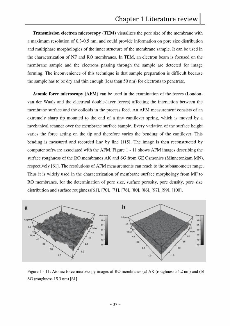
Atomic force microscopy (AFM) can be used in the examination of the forces (London-
van der Waals and the electrical double-layer forces) affecting the interaction between the
membrane surface and the colloids in the process feed An AFM measurement consists of an
extremely sharp tip mounted to the end of a tiny cantilever spring which is moved by a
mechanical scanner over the membrane surface sample Every variation of the surface height
varies the force acting on the tip and therefore varies the bending of the cantilever This
bending is measured and recorded line by line [115] The image is then reconstructed by
computer software associated with the AFM Figure 1 - 11 shows AFM images describing the
surface roughness of the RO membranes AK and SG from GE Osmonics (Minnetonkam MN)
respectively [61] The resolutions of AFM measurements can reach to the subnanometer range
Thus it is widely used in the characterization of membrane surface morphology from MF to
RO membranes for the determination of pore size surface porosity pore density pore size
distribution and surface roughness[61] [70] [71] [76] [80] [86] [97] [99] [100]
Figure 1 - 11 Atomic force microscopy images of RO membranes (a) AK (roughness 542 nm) and (b)
SG (roughness 153 nm) [61]
Chapter 1 Literature review
~ 38 ~
It has been reported that surface roughness has an important effect in membrane fouling
behaviour [80] [123] Because of the ridge-and valley structure of rough membrane surfaces
colloids are thought to be preferentially transported into the valleys (path of least resistance)
which results in ldquovalley cloggingrdquo and hence in a more severe flux decline in comparison with
smooth membranes
The choice of characterization method is generally made based on the problem to which an
answer is required and on the time cost and resources available However the best
knowledge is always obtained by combining results from different characterization methods
13 Surfactants
131 Development and applications
Surfactants may be from natural or synthetic sources The first category includes naturally
occurring amphiphiles such as the lipids which are surfactants based on glycerol and are vital
components of the cell membrane [124] [125] Soaps remained the only source of natural
detergents from the seventh century till the early twentieth century with gradually more
varieties becoming available for shaving and shampooing as well as bathing and laundering
In 1916 in response to a World War I-related shortage of fats for making soap the first
synthetic detergent was developed in Germany Known today simply as detergents synthetic
detergents are washing and cleaning products obtained from a variety of raw materials [126]
[127] Nowadays synthetic surfactants are essential components in many industrial processes
and formulations such as household detergents personal care formulations industrial and
institutional washing and cleaning as well as numerous technical applications such as textile
auxiliaries leather chemicals agrochemicals (pesticide formulations) metal and mining
industry plastic industry lubricants paints polymers pharmaceutical oil recovery pulp and
paper industry etc [8] They are also occasionally used for environmental protection eg in
oil slick dispersions [9]
The production of surfactants has increased over the last decades In 2000 25 Mtyear of
surfactants were produced in Western Europe countries In 2011 total annual tonnage of
surfactants produced in Western Europe had already increased to 295 Mtyear according to
the CESIO (Comiteacute Europeacuteen des Agents de Surface et leurs intermediaries Organiques)
Chapter 1 Literature review
~ 39 ~
statistics for surfactantsrsquo production in β011 (CESIO Statistics β011 β01β) The statistics
surveyed Western European companies representing more than 50 surfactants manufacturers
70 of the European surfactantsrsquo market (CESIO News ndash Dec 2012) As it can be seen in
Figure 1 - 12 non-ionic surfactants are the most produced type of surfactant followed by
anionic ones The production of cationic and amphoteric surfactants is quite lower
Figure 1 - 12 Annual production of surfactants in Western Europe from 2000 to 2011 (CESIO
Statistics 2011 Dec 2012)
132 Definition of surfactants
Surfactant is an abbreviation for surface active agent which literally means active at a surface
The molecular structure of surfactants is amphiphilic consisting of both non polar
(hydrophobic or tail) and polar (hydrophilic or head) parts as shown in Figure 1 - 13 When
dissolved in a solvent surfactants tend to adsorb (or locate) at interfaces with hydrophilic
head retaining in the polar phase (usually water) while the hydrophobic tail facing the apolar
phase thereby altering significantly the physical properties of those interfaces The driving
force for a surfactant to adsorb at an interface is to lower the free energy of that phase
boundary [128]
Chapter 1 Literature review
~ 40 ~
Critical micelle concentration (CMC) is the concentration below which virtually no
micelles are detected and above which virtually all additional surfactant molecules form
micelles And aggregation number is the number of surfactant molecules present in a micelle
once the CMC has been reached
Figure 1 - 13 Amphiphilic structure of surfactants The head corresponds to the hydrophilic part of the
surfactant molecule which is polar while the tail represents the hydrophobic group of the surfactant
molecule which is apolar
133 Chemical structure and classification
Chemical structure of surfactants
Numerous variations are possible within the structure of both the head and tail group of
surfactants The hydrophobic group of the surfactant structure is usually a single or double
straight or branched hydrocarbon chain but may also be a fluorocarbon or a halogenated or
oxygenated hydrocarbon or siloxane chain Typical hydrophobic groups are listed in Table 1 -
4 The hydrophilic part of the structure may be represented by non-ionic polar groups or ionic
groups as listed in Table 1 - 5
Surfactants are classified by the polar head group
Chapter 1 Literature review
~ 41 ~
Depending on the nature of the hydrophilic head group surfactants are therefore classified
into four basic types anionic cationic non-ionic and zwitterionic surfactants (see Figure 1 -
13)
Table 1 - 4 Common hydrophobic groups used in commercially available surfactants [7]
Group General structure
Natural fatty acids CH3(CH2)n n = 12-18
Olefins CH3(CH2)nCH=CH2 n = 7-17
Alkyl benzenes CH2(CH2)nCH3
n = 6-10 linear or branched
Alkyl aromatics
R
R
CH2(CH2)nCH3
n = 1-2 for water soluble
n = 8 or 9 for oil soluble surfactants
Alkyl phenols CH2(CH2)nCH3
HO
n = 6-10 linear or branched
Polyoxypropyrene CH3CHCH2O(CHCH2)n
X CH3
n = degree of oligomerisation X = oligomerisation initiator
Fluorocarbons CF3(CF2)nCOOH n = 4-8 linear or branched or H terminated
Silicones
(SiO)n
CH3
CH3O
CH3
CH3
Anionic surfactants are those molecules of which the surface-active portion bears a
negative charge Common anionic surfactants are sulfonic acid salts sulfuric acid ester salts
carboxylic acid salts phosphoric and polyphosphoric acid esters and perfluorocarboxylic
acids
Chapter 1 Literature review
~ 42 ~
Cationics contain a hydrophilic group positively charged for example long-chain amines
and their salts acylated diamines and polyamines and their salts quaternary ammonium salts
Nonionics bear no appearent ionic charge in their hydrophilic part which include a highly
polar (non charged) moiety such as monoglyceride of long-chain fatty acid
polyoxyethylenated alkylphenol polyoxyethylenated alcohol
Table 1 - 5 Common hydrophilic groups found in commercially available surfactants [7]
Class General structure
Sulfonate R-SO3-M+
Sulfate R-OSO3-M+
Carboxylate R-COO-M+
Phosphate R-OPO3-M+
Ammonium RxHyN+X-(x = 1 ndash 3 y = 4 ndash x)
Quaternary ammonium R4N+X-
Betaines RN+(CH3)2CH2COO-
Sulfobetaines RN+(CH3)2CH2 CH2SO3-
Polyoxyethylene(POE)
R-OCH2CH2(OCH2CH2)nOH
Polyols Sucrose sorbitan glycerol ethylene glycol etc
Polypeptide R-NH-CHR-CO-NH-CHRrsquo-CO-hellip-COOH
Polyglycidyl R-(OCH2CH[CH2O]CH2)n-hellip-OCH2CH[CH2OH]CH2OH
Zwitterionics (or amphoterics) carry both positive and negative charges in the head group
Long-chain amino acid and sulfobetaine are the most encounted examples of this type of
surfactants
With the continuous search for improving surfactant properties and for enhanced
biodegradability new structures have recently emerged that exhibit interesting synergistic
interactions or enhanced surface and aggregation properties These novel surfactants have
attracted much interest and include the catanionics bolaforms gemini (or dimeric)
surfactants polymeric and polymerisable surfactants [7]
Chapter 1 Literature review
~ 43 ~
134 Properties of surfactants
1341 Surfactant micellization
When dissolved in water amphiphilic surfactants that contain hydrophobic groups distort the
structure of water and therefore increase the free energy of the system To minimize the free
energy of the solution they concentrate at the surface by orienting their hydrophobic groups
away from the solvent (water) or they self-assemble into clusters with their hydrophobic
groups directed toward the interior of the cluster and their hydrophilic groups directed toward
the water when total surfactant concentration rises to the CMC
Figure 1 - 14 Surfactant monomers and micelle formation in water
Above their critical micelle concentration there is equilibrium between monomers small
aggregates and micelles Any further increase of total surfactant concentration results in the
formation of more micelles and the concentration of free surfactants keeps constant around
the CMC (see Figure 1 - 14) Surfactants aggregate spontaneously form a wide variety of
assemblies ranging from micelles rodlike structures and bilayers to more complex phases
such as cubic phases The micellar aggregation number and shape of the surfactant aggregates
Chapter 1 Literature review
~ 44 ~
depend on the type of surfactant (the volume VH occupied by the hydrophobic groups in the
micellar core the length of the hydrophobic group in the core lc and the cross-sectional area
a0 occupied by the hydrophilic group at the micelle-sotution interface) and the solution
conditions
The thermodynamics of micellization is described in details in several reports [7] [129]
[130] The surfactant solution can be considered as a multi-component system consisting of
water singly dispersed surfactant molecules and aggregates of all possible shapes and
aggregation numbers Nagg At equilibrium the chemical potential of free monomers must
equal the chemical potential of surfactants involved in each aggregate μagg (Equation 1 - 18)
where are the standard state chemical potentials and the molar fraction of
the surfactant aggregate with aggregation number i and of the surfactant monomers
respectively [7] Every addition of a surfactant molecule to the solution leads an increase of
free energy by the interplay of molecular interactions with water The CMC is the threshold
concentration at which the chemical potential of the free monomer becomes equal to that of
monomers involved in micelles
The surfactant self-assembly process depends primarily on surfactant architecture the
solvent the presence of added components (ie co-surfactants or salts) and temperature The
micellization of surfactant cause sharp breaks at the CMC in the physical properties that
depends on size or number of particles in solution including electrical conductivity surface
or interfacial tension etc [7] This self-aggregation process of surfactants is of fundamental
importance to many biological and industrial processes
1342 Surfactant adsorption at solid-liquid interface
The surfactants have strong tendency to adsorb at interfaces in an oriented way The
adsorption of surfactants at the solid-liquid interface is strongly influenced by several factors
[131]
ndash the nature of the structural groups on the solid surface the charged sites or essentially
nonpolar groupings and the constitution (eg the atoms and functional groups) of these sites
or groupings
Chapter 1 Literature review
~ 45 ~
ndash the molecular structure of the surfactant being adsorbed the charge of the hydrophilic
part and the structure of the hydrophobic tail group (ie length of the straight or branched
chain aliphatic or aromatic hydrocarbons) of the surfactant molecule
ndash the chemical and physical conditions of the aqueous solution the pH temperature the
presence of any electrolytes or other additives (alcohol urea etc)
13421 Mechanisms of surfactant adsorption at solid-liquid interface
The mechanisms by which surfactants may adsorb onto solid surfaces from aqueous solutions
are determined together by the factors as listed above Several mechanisms are briefly
described as follows
ndash Ion exchange between surfactant ions and similarly charged counterions adsorbed onto
the solid surface from the solution
ndash Ion pairing of surfactant ions from solution onto oppositely charged sites of the solid
surface which has been occupied by counterions
ndash Acid-base interaction via either Lewis acid-base reaction or hydrogen bonding
between surfactant molecules and the solid surface
ndash Attraction by polarization of electrons This may occur if the solid surface contains
strongly positive sites and there are electron-rich aromatic nuclei in the surfactant molecule
ndash - interaction between aromatic nuclei of the surfactant molecule and of the solid
surface if both contain such function group
ndash Adsorption by London-van der Waals dispersion forces between surfactant and solid
surface molecules
ndash Hydrophobic bonding between tail groups of the surfactant molecules drives them to
escape from water and onto the solid surface while hydrophobic bonding between the tail
groups of the surfactant molecules and hydrophobic sites on the solid surface
In aqueous systems the structures formed are determined by the interaction of the
surfactant molecules with the solid surface in order to minimize exposure of the hydrophobic
groups to water The organization and structure of surfactant molecules or aggregates onto
solid surfaces could be observed from scanning probe microscopic techniques like AFM
Chapter 1 Literature review
~ 46 ~
fluorescence quenching and neutron reflectivity [132] [133] The most observed structures of
surface aggregates on a variety of solid surfaces have been reported to be hemimicelles
admicelles monolayers hemispherical bilayers and cylinders [7] [134] [135] [136] The
orientation of the adsorbed surfactants onto a smooth nonporous planar solid surface could be
determined from the contact angle measurements (Section 1253) The comparison of the
obtained contact angles before and after surfactant adsorption could also provide information
of the modification of membrane hydrophilicity due to surfactant adsorption Orientation of
the surfactants with their hydrophilic groups predominantly away from the solid surface will
make it more hydrophilic than before the adsorption of surfactants [7]
In this thesis since we focus on the active layer of RO membrane surface the majority of
which available in the market is made of polyamide (see Figure 1 - 6) the probable
interactions between the membrane surface and the surfactant molecules could be [128]
ndash Electrostatic interactions the carboxylic acid (ndashCOOH) and free amine (ndashNH2) groups
that are not engaged in the cross-linking of the amide bond may be ionized when in contact
with a surfactant solution carrying a negative or positive charge thus they are possible to
interact with the ionic surfactants through electrostatic forces
ndash Hydrogen bonding this may occur in the carboxylic acid (ndashCOOH) and free amine (ndash
NH2) groups with the surfactants
ndash - interaction between aromatic nuclei of the membrane surface and aromatic
surfactants
ndash Hydrophobic interactions between surfactants and the hydrophobic sites on the
membrane surface
ndash Mutual attraction (via hydrophobic bonding) of surfactant molecules with those
adsorbed onto the membrane
ndash London-van der Waal forces by the amide bond
ndash Lewis acid-base interactions this may occur in the carboxylic acid (ndashCOOH) and free
amine (ndashNH2) groups
13422 Adsorption isotherms at solid-liquid interface
Chapter 1 Literature review
~ 47 ~
The adsorption isotherm is a mathematical expression that relates the concentration or amount
of adsorbate on the solid surface to its equilibrium concentration in the liquid phase It is
usually used to describe the surfactant adsorption at the liquid-solid interface The information
on the solid surface such as the area covered by surfactant and the maximum surfactant
adsorption can be measured After complementary analysis the change of solid surface
properties by the surfactant adsorption the equilibrium adsorbed surfactant morphology as
well as the mechanism by which the surfactant is adsorbed at the interface could be predicted
The most frequently used models for the adsorption isotherm are linear adsorption
isotherm Langmuir and Freundlich adsorption isotherm
Linear adsorption isotherm
The linear adsorption isotherm formally resembles Henryrsquos law so it is also called Henryrsquos
adsorption isotherm In this model the amount of the adsorbate onto solid surface is directly
proportional to its concentration in solution
(Equation 1 - 19)
where Qads is the amount of surfactant adsorption onto the adsorbent mol m-2 or g m-2
KH is the Henry adsorption constant L m-2
Ceq is the equilibrium concentration of the surfactant in solution mol L-1
The linear isotherm can be used to describe the initial part of many practical isotherms for
low concentrationssurface coverage or very low interaction energy between the adsorbate and
the adsorbent
Langmuir adsorption isotherm (L type)
This model is commonly used to the surfactant adsorption from aqueous solutions expressed
by [100][131]
(Equation 1 - 20)
where Qads = the surface concentration of the surfactant per unit area (or per unit mass) of the
solid adsorbent in mol m-2 (or mol g-1) at monolayer adsorption
Chapter 1 Literature review
~ 48 ~
C = the concentration of the surfactant in the liquid phase at adsorption equilibrium in
mol L-1
KL = the Langmuir constant in L mol-1 containing information related to the adsorbate-
adsorbent interaction free energy in the system 1KL = 55γ exp (ΔG0RT) at absolute
temperature T in the vicinity of room temperature and where ΔG0 is free energy of adsorption
at infinite dilution
The application of Langmuir-type model is valid in theory only when the following
restrictions are met (1) the solid surface is homogeneous consisting of adsorption sites (2) all
adsorbed surfactants interact only with one site and not with each other (3) the adsorption
film is monomolecular This model also has been very useful for studying adsorption systems
between surfactants and polymeric materials
Xiarchos et al has successfully fitted their experimental data from the adsorption of
nonionic surfactants onto UF membranes during filtration to the following Langmuir model
[100]
(Equation 1 - 21)
where Ceq = the concentration of the surfactant in the liquid phase at adsorption
equilibrium in mol L-1
Qadmax = maximum adsorption of the surfactant per unit mass of the UF
membranes in mol m-2 at monolayer adsorption
KL = the Langmuir constant in L mol-1 containing information related to the
adsorbate-adsorbent interaction free energy in the system
S type adsorption isotherm
Due to attractive lateral interactions between surfactant molecules the Langmuir isotherm
may become S-shaped or stepped [137] A two-step adsorption mechanism has been proposed
in the first step the surfactant molecules are adsorbed as individual molecules or ions then in
the second step there is a sharp increase in the adsorption as surface aggregates form through
interaction of the hydrophobic chains among the surfactant molecules
Chapter 1 Literature review
~ 49 ~
(Equation 1 - 22)
where Qinfin = the limiting surfactant adsorption at high concentration C
KS = the equilibrium constant of the surface aggregation process
ns = the average aggregation number of the surface aggregate as a general adsorption
isotherm
(Equation 1 - 22 can be transformed to the linearized expression as follows
(Equation 1 - 23)
The values of KS and ns could be obtained from a plot of log [Qads (Qinfin - Qads)] versus log
C if there is a linear relationship between them If ns gt 1 this means surfactant aggregation at
the solid surface occurs
The adsorption isotherm of an ionic surfactant on an oppositely charged solid surface
usually follows a more complicated mechanism This typical adsorption isotherm can be
subdivided into four regions when plotted on a log-log scale (see Figure 1 - 15) [138] In the
first region the surfactants adsorb as individual molecules on single surface sites at low
concentrations The amount of adsorbed surfactants is very low and the interaction between
adsorbed surfactants is negligible thus this first region is governed by Henryrsquos law The
second region shows a sudden increase of adsorption due to the formation of primary
aggregates known as hemimicelles when the critical aggregation concentration (CAC) is
reached In the third region the solid surface is neutralized by the adsorbed surfactant ions
the electrostatic attraction is no longer operative and adsorption takes place due to lateral
attraction alone with a weaker increasing up to a plateau region with constant adsorbed
amount The plateau indicates that the surfactant monomer activity becomes constant and any
further increase in concentration contributes only to the micellization in solution and it does
not change the adsorption quantity In some cases the fourth region can contain a weak
maximum before arriving at the plateau The isotherm of surfactants on hydrophobic surfaces
as well as the form of adsorbed surfactant molecules is proposed in Figure 1 ndash 15 [13]
Chapter 1 Literature review
~ 50 ~
Figure 1 - 15 Schematic presentation of typical four-region adsorption isotherm [139]
Figure 1 - 16 Adsorption of surfactants on hydrophobic surface a surfactant monomers b surfactant
micelles c isolated adsorbed surfactant monomers d surface aggregates[13]
Chapter 1 Literature review
~ 51 ~
Freundlich Adsorption Isotherm
The Freundlich equation is an empirical expression with the assumption that the adsorbent has
a heterogeneous surface composed of adsorption sites with varying energy [140] It represents
the amount of a solute on the adsorbent to the concentration of the solute in the liquid phase
at different solution concentrations This equation is expressed as follows
(Equation 1 - 24)
where is the amount of particle adsorption onto the adsorbent mol m-2 or g m-2
Kf and nf are empirical constants for a given adsorbate and adsorbent pair at a
particular temperature with nf generally greater than unity
Ceq is the equilibrium concentration of the adsorbate in solution mol L-1
Even though this model does not describe clearly the physical phenomenon it can be
applied to the case with a heterogeneous surface where there are different adsorption sites for
attachment of the solute Since the adsorbent would not be saturated by the adsorbate in this
model the infinite surface coverage indicates multilayer sorption of the surface
Freundlich isotherm could be rewritten to the logarithmic form and a linear relationship
could be obtained as follows
(Equation 1 - 25)
135 Environmental effects of surfactant
Due to the significant production and the widespread use of surfactant-based formulations
wastewaters containing surfactants are generally encountered Direct discharge of
wastewaters containing surfactant into rivers may cause foam formation and may origin
anomalies to algae growth and toxicity to aquatic organisms [127] If sent to a wastewater
treatment plant they can cause disruption of the plant preventing sewage from being treated
and forcing the plant to discharge raw sewage
Chapter 1 Literature review
~ 52 ~
136 Membrane filtration of surfactants
Various organic materials such as phenols surfactants pesticides herbicides aromatic
hydrocarbons among many others are typically found in industrial effluents Specially
surfactants are usually present in domestic wastewater food engineering discharged effluents
and cleaning solutions for membrane stacks used in water treatment Those substances are
examples of highly stable organic pollutants Their persistence to the environment has been
demonstrated and many times the symptoms of contamination may not manifest themselves
until several generations after initial contact with the chemical of concern Thus wastewaters
containing such non-biodegradable pollutants need to be treated and pollutants removed to
avoid associated environmental pollution
Surfactants have been extensively used in membrane processes such as pretreatment of
membranes with surfactant solutions removal of low molecular weight organic toxic
compounds and metal ions from solutions by micellar-enhanced ultrafiltration (MEUF)
Removal of surfactants and estimation of interactions at surfactant membrane interface have
also been studied In this work we focus on the removal of surfactants from wastewaters by
membrane filtration processes
Most of the membrane filtration studies published to date concerning about the treatment
of surfactant solution have been carried out with crossflow UF which have been widely used
to remove surfactants from wastewaters The surfactant micelles are retained by the
membrane while monomers are too small and pass through the membrane The permeate
concentration of surfactants is close to their CMC If the surfactant concentration is lower
than the CMC where the surfactant exist mainly as monomers nanofiltration has been
suggested as an effective removal process [141] Studies on the RO processes applied in
removing surfactants from wastewaters are rather limited in the literature The removal of
surfactants could be higher than 90 and even 99 for NF and RO respectively [142] [143]
[144]
Membrane fouling during filtration of surfactant solutions has been studied mainly in the
case of UF In general surfactants may cause severe fouling problems and thus decrease the
membrane flux The reason for the flux decline in some cases has been due to concentration
polarization caused by retained micelles Another reason for the decrease of permeate flux has
Chapter 1 Literature review
~ 53 ~
been attributed to adsorption of surfactant molecules in the membrane pores or on the
membrane surfaces through hydrophobic andor electrostatic interactions The flux decline is
thought to be related to the adsorbed amount [112] But in some cases the adsorption of
surfactants on the membrane surface increased membrane hydrophilicity due to the
orientation of adsorbed surfactant molecules leading to a higher permeate flux [145] [146]
Therefore they are also used in the cleaning solution for surface modification to improve
membrane performance [147] [148] [149] [150]
The orientation of adsorbed surfactant molecules or layers is determined by the interactions
between surfactant molecules and membrane surface andor between surfactant molecules
which may influence the membrane surface properties leading to deterioration or
improvement of membrane performance The adsorption structure of the surfactants on the
membrane surface has been reported as a close compact structure (eg monolayer) at high
concentrations with the hydrophilic head groups or hydrophobic tail groups facing towards
the aqueous solution thus modifying the surface properties of the membrane and
consequently influencing the membrane performances (ie transport and separation
properties) while at low concentrations or at the early stage of adsorption the surfactant
molecules lay parallel to the membrane surface
There are examples of surfactant solution in connection with different membrane processes
MF of nonionic anionic and cationic surfactant [145] [151] UF of nonionic and ionic
surfactants[9] [100] [129] [141] [145] [146] [152] [153] [154] [155] [156] [157] [158]
[159] [160] micellar-enhanced ultrafiltration [161] [162] [163] NF of nonionic anionic
and cationic surfactants [112] [156] [164] [165] surfactant enhanced NF and RO
membranes [147] RO of different surfactants [144] [166] [167] [168] [169] [170] [171]
anionic surfactant (SDS) effects on the RO membrane (thin-film composite polyamide) [148]
[149] cleaning of RO membrane using anionic surfactant (SDS) [150] shear induced
surfactant filtration [172] Since the properties of solutions of surfactants change markedly
when micelle formation occurs surfactant was used at concentrations below its CMC in
several filtration experiments [9] [100] [129] [145] [152] [153] [154] [155] [156] [157]
[158] [159] [160] Some membrane processes for the removal of a variety of surfactants
from solution in the literature are summarized in Table 1 - 6
Chapter 1 Literature review
~ 54 ~
Table 1 - 6 a Membrane filtration of surfactants in literature microfiltration
Membrane Surfactant Operating
condition
Interesting results Reference
MWCO Composition Composition
Charge CMC
(25 degC)
Concentration
MF 0β μm cellulose
acetate
Linear alkyl benzene sulfonate
(C13H27C6H4SO3H)
Anionic
20 mM
0 -10 mM ΔP = 150 kPa T = 30 degC V = 118m s-1
(1) The removal of surfactants is attributed to
the formation of a secondary membrane on
the surface and within the pores of the MF
membrane
(2) Increase in transmembrane pressure and
pore size of the membrane decreased the
surfactant rejection rates
(3) Increase in cross-flow velocity increased
the rejection rate
[151]
Cetyl trimethyl ammonium bromide
(C19H42NBr)
Cationic 092 mM 0 -10 mM
Chapter 1 Literature review
~ 55 ~
Table 1 - 6 b Membrane filtration of surfactants in literature ultrafiltration
PES Polyethersulfone PS Polysulfone C Regenerated cellulose CA Cellulose acetate PA Aromatic polyamide PVDF Poly(vinylidene fluoride)
Membrane Surfactant Operating
condition
Interesting results Ref
MWCO
(KDa)
Composition Composition
Charge CMC
(25 degC)
Conc
UF 51030 PES SDS Sodium dodecyl sulfate C12H25SO4Na
Anionic 783 mM
0017 ndash
208 mM
(lt CMC)
P = 005 020
MPa
T = 25 degC
pH = 7
(1) Hydrophobic membranes are more susceptible to fouling than
hydrophilic membranes
(2) Fouling would be increased with the increase in membrane
cut-off
(3) Increasing the pressure will cause an increase in permeability
but a slight decrease in surfactant rejection
(4) Membrane permeability and SDS rejection decreased with the
increase in the surfactant concentration
[141]
51030 PS
51030 C
51030 CA
51030 PA
UF
10 hydrophilic
PES
SDBS Sodium dodecyl benzene
sulfonate
C12H25(C6H4)SO4Na
anionic 188 mM CCMC =
05 ndash 5
(1) The effect of the concentration polarization was greatly
reduced due to the high shear rates on the membrane
(2) The permeate flux rises with increasing the surfactant
concentration
(3) Compared to new membranes a higher surfactant
concentration gives a bigger increase in the hydrophilicity of
PES membrane after treated with the surfactant solution
(4) The surfactant retention decreased as feed concentration rose
due to the existence of sub-micellar aggregates and higher
permeate flux
[146]
Chapter 1 Literature review
~ 56 ~
UF 20 PS
(GR 61 PP)
Tritons
Alkylphenol ethoxylates
C8H17(C6H4)O(CH2CH2O)n
H
n = 581012
Non-ionic 015 ndash 037
mM
C le CMC
(CCMC =
01 033
05 075
10)
ΔP = 005 ndash
020 MPa
T = 20 degC
pH = 7
v = 4 m s-1
and 25 m s-1
(1) The hydrophobic PS membrane experienced a sharp flux
decline in contact with surfactant solution because of the
interaction between the membrane material and the
hydrophobic part of the surfactant molecules leading to
adsorption probably within the membrane pores
Concentration polarization is unlikely in this work since no
significant flux reduction was observed for CA membrane
The hydrophilic membrane showed weaker interactions with
non-ionic surfactants in this study
(2) The flux of the surfactant solution was a linear function of
pressure
(3) As the surfactant concentration approaches the CMC the most
hydrophobic surfactant causes the greatest decline in flux The
surfactant with intermediate hydrophobicity shows an
intermediate behavior
[152]
20 CA
(CA 600 PP)
Dobanol CxH2x+1O(CH2CH2O)nH
n = 5678
08 ndash 10 mM
UF
20 PS
(GR 61 PP)
Tritons Alkylphenol ethoxylates
C8H17(C6H4)O(CH2CH2O)n
H
n = 81012
Non-ionic 0265 mM
028 mM
037 mM
C le CMC
(CCMC =
01 033
05 075
10)
T = 20 degC
pH = 7 and
pH = 2
(1) The surfactant adsorption on the membranes depends on the
chemical composition and structure of both the surfactant and
the membrane used as both the chemical composition and
structure determine the type of interactions controlling this
adsorption The interactions are due to intermolecular and
interfacial forces which develop between the substrate (in this
case membrane) and the surfactant
(2) The adsorption of surfactant onto the hydrophobic membranes
is larger than hydrophilic membranes
(3) Upon increasing the hydrophilicity of the nonionic surfactant
by increasing the ethylene oxide groups (EO) the adsorption
decreases
(4) In the early stages of adsorption surfactant molecules lie flat
[153]
20 PVDF-
hydrophobic
(FS 61 PP)
Chapter 1 Literature review
~ 57 ~
on the membrane surface as the concentration increases close
packed assembly will result by orienting perpendicular to the
surface with hydrophilic head groups towards the aqueous
phase
20 CA
(CA 600 PP)
Dobanol-
series
surfactant
s
CxH2x+1O(CH2CH2O)nH
n = 568
x = 91011
08 mM
09 mM
10 mM
20 PVDF-
modified
(ETNA 20 A)
UF 6
20
500
PS Triton X-
100
Nonionic 024 mM CCMC =
01 04 10
40
ΔP = 05
MPa
T = 25 degC
pH = 7
v = 075 and
105 m s-1
(1) The flux declines of the hydrophobic membranes were found
to be much more significant than that of the hydrophilic ones
since the adsorption of surfactants is more pronounced for
hydrophobic than for hydrophilic solids
(2) The influence of the anionic surfactants on the low cut-off PS
membranes was highly irregular as the flux increased
markedly at the CMC The impurities in the solution caused
the divergent performance of the membranes
(3) Retention of the ionic surfactants was quite high even at low
concentrations
(4) The performance of the hydrophobic membranes was
determined by both the material and the MWCO of the
membranes
[154]
6
20
PVDF oleate
and SDBS
Potassium oleate and
sodium dodecylbenzene-
sulphonate
anionic 09 mM
110 mM
8
20
CA CTAB Hexadecyltrimethylammoni
um bromide
cationic 092 mM
Chapter 1 Literature review
~ 58 ~
Table 1 - 6 c Membrane filtration of surfactants in literature nanofiltration
PES Polyethersulfone PS Polysulfone C Regenerated cellulose CA Cellulose acetate PA Aromatic polyamide PVDF Poly(vinylidene fluoride)
Membrane Surfactant Operating
condition
Interesting results Ref
MWCO
(Da)
Composition Composition Charge CMC
(25 degC)
Conc
NF 190 Desal 51HL
NF 270
NTR 7450
NFPES10
Neodol
SDBS
cetrimide
RO(CH2CH2O)nH
CH3(CH2)11C6H4SO3Na
CH3(CH2)15N(CH3)3Br
Nonionic
Anionic
cationic
1150 mg L-1
2320 mg L-1
1320 mg L-1
20 ndash 70 mg
L-1
ΔP = 8 bar
T = 20 degC
pH = 6
v = 45 m s-1
(1) Membrane performance decreases with increasing
concentration
(2) The flux decline is related to the adsorbed amount of
surfactants
(3) The adsorption of surfactants is determined by the
hydrophobic andor electrostatic (in the case of ionic
surfactants) interactions with the membrane Hydrophilic
membranes have less surfactant adsorption amount than
hydrophobic ones
(4) The nonionic surfactant can undergo chain folding and
penetrate into and be adsorbed in the large pores of the
hydrophobic membrane causing large amount of adsorption
(5) The retentions of ionic surfactants did not change
significantly while the retention of nonionic surfactant
decreased with increasing concentration
[112]
155
310
1200
Chapter 1 Literature review
~ 59 ~
NF 400 PES
(NF PES 10)
LABS
SLES
NPE
Linear alkyl benzene
sulfonate
R-C6H4SO3H
Sodium dodecylether
sulfate
R-O-(CH2CH2O)2-SO3Na
Nonylphenol ethoxylate
(C4H9)2CHC6H4(OC2H4)9O
H
Anionic
Anionic
Nonionic
064 g L-1
030 g L-1
006 g L-1
C lt CMC
For single
surfactant
solutions C
= 50 200
500 mg L-1
for LABS
SLES and
NPE
respectively
ΔP = 12 bar
T = 18 plusmn 1 degC
v = 30 L min-
1
pH = 30 57
58 and 30 for
LABS SLES
NPE and
mixture
solution
respectively
(1) The rejection of surfactants and flux decline took place due to
the adsorption of surfactants onto both surface and pore walls
which is depending on MWCO and contact angles of the
membranes
(2) A secondary membrane layer formed on the surface of N 30F
and XN 45 membrane in addition to the surfactant aggregates
which occurred on the surfaces of all membranes A large
number of small aggregates formed on N 30 F (smooth and
negatively charged) while less aggregates with larger sizes
formed on NF PES 10 Surfactant aggregates accumulated
densely on XN 45 surface which is neutral and rough
(3) Anionic surfactants are bond to membrane surface through
hydrophobic attraction stronger than electrostatic repulsion
on membrane surfaces with negative charge
(4) The most surface fouling occurred on XN 45 membrane for
anionic surfactants since anionic surfactants consisting of
long chains are able to fold to a substantial degree thus could
penetrate into the pores of this membrane with a MWCO
smaller than the molecular weights of anionics at relatively
low rejections
[164]
1000 PES
(N 30F)
200 PA ( XN 45)
Chapter 1 Literature review
~ 60 ~
Table 1 - 6 d Membrane filtration of surfactants in literature reverse osmosis
PES Polyethersulfone PS Polysulfone C Regenerated cellulose CA Cellulose acetate PA Aromatic polyamide PVDF Poly(vinylidene fluoride)
Membrane Surfactant Operating
condition
Interesting results Ref
Composition Composition Charge CMC
(25 degC)
Conc
RO CA-10
CA-75
CA-90
FT 248
BAC
Tetraethylammonium-
perfluorooctane sulfonate
Benzalkonium chloride
Anionic
Cationic
011 mM ΔP = 10 ndash 40
bar
T = 20 plusmn
03 degC
v = 09 L min-
1
pH = 3
(1) The flow reduction caused by the anionic surfactant is
reversible
(2) A gel layer is formed on the membrane at a very low
concentration for BAC the amount of BAC adsorption on the CA-
10 membrane increases from 10 to 42 g m-2 with the applied
pressure increasing from 10 to 40 bars The corresponding values
for the CA-75 membrane were 20 and 35 g m-2 respectively
[171]
RO SG1812C
-28D
Thin-film PA - Fluorinated surfactant Anionic - 23 ndash 417 mg
L-1
470 mg L-1
140 mg L-1
ΔP = 20 bar
T = 25 degC
v = 0084 m s-
1
pH = 68 75
82
(1)Pure water permeability was 2L h-1 m-2 bar-1
(2)Surfactant retention rates were higher than 999 and flux
decline is significant
(3)Mass balance showed that certain quantity of surfactants was
adsorbed onto the membrane surface
(4)Flux permeability decreased with increasing the surfactant
concentration
[144]
RO E-398-3 Modified CA ABS Sodium dodecylbenzene
sulfonate
anionic 140 mM
C lt CMC ΔP = 40 bar
v = 250 mL
min-1
(1)The rejection of ionic surfactants was larger than that of
nonionic surfactants especially at concentrations below CMC
(2)The flux decreased with the increase of molecular weight for
[166]
Chapter 1 Literature review
~ 61 ~
TDBNC Tetradecylbenzylammoni
um chloride
Cationic 420 mM nonionic surfactants
(1) The CMC affected the transport significantly of nonionic
surfactants
(2) Concentration polarization on the membrane surface could be
predicted by taking into account the difference between
surfactant fluxes below and above CMC
NP-10
NP-16
NP-27
Polyoxyethylene
nonylphenyl ether
Nonionic 00527 mM
0068 mM
0144 mM
RO CA Negatively
charged CA
BAC Benzalkonium chloride Cationic 011 mM ΔP = 5 ndash 40
bar
T = 20 plusmn 1 degC
v = 09 L min-
1
(1) The adsorption of surfactants on the membrane surface
caused a slight decrease in the flux
(2) At CMC the surfactant rejection increased which could be
explained by a change in the activity By adsorption of the
surfactants at the pore walls of the membranes the water
transport is reduced and the fixed charge in the pores
increased by adsorption of charged surfactant leading to a
more pronounced Donnan exclusion of the solutes
[168]
SPSU Sulfonated
PS(negative)
FT 248 Tetraethylammonium Anionic
RO FT-30 Thin film
composite PA
SDS Sodium dodecyl sulfate Anionic 82 mM 10 mM 01 M NaCl
02 ΔP = 5 ndash 40
bar
pH = 3 ndash 9
T = 20 degC
v = 09 L min-
1
1 The surfactants were found to readily adsorb to the membrane
surface and markedly influence the membrane surface charge
The negatively-charged sulfate functional groups of the
surfactant molecules cause the membrane to become more
negatively charged
2 The formation of surfactant hemimicelles on the membrane
surfactant resulted in a secondary filtration layer on the
membrane surface which caused decreased flux and
increased salt rejection at low pH
[148]
CG CA
Chapter 1 Literature review
~ 62 ~
From the table we can see that although various membrane filtrations have been
undertaken the majority of these works focused on membrane performance There has been
no work studying the adsorption isotherm of surfactants on the membrane surface due to
operating conditions such as continuous pressure as well as the tangential flow along the
membrane surface In addition the characteristics of the morphology or surface organization
of these amphiphilic molecules during membrane filtration seem to have not yet been realized
A fundamental work on this aspect is needed for providing enough information on the
filtration process
14 Membrane filtration
The main limitations to the wild spread of membrane processes and its performance
optimization are the membrane fouling leading to flux decline the cleaning and the selectivity
Recently the scientists look for a better understanding of the local mechanisms and modeling
has played an important role [101] [173] [174] [175] [176] [177] The porous media
constituting the membrane was a black box few years ago and simple hypothesis and
modeling are still used to describe what happens on or inside the membrane resistance-in-
series model concentration polarization cake formation pore blocking or pore constriction
[178] But the local description of the porous media is now more and more studied because
this is the place where everything happens Membranes are complex structures organic or
mineral with variable compositions During the filtration they can generate various
interactions (hydrogen bonding Van der Waal Lewis ionic exchange etc) depending on the
membrane and the composition of the complex solution to treat A better understanding of the
local interaction could help to propose new strategies to enhance the performances of
membrane processes to reach an efficient separation limiting the energy cost due to flux
decline and limiting cleaning periods
The membrane characterization and the deepen study of the interaction have been
published in recent papers dealing with fouling life time [179] mapping of fouling etcThe
main difficulty is the submicronic size of the structure to analyze analytical methods are still
limited It is neither possible at the moment to describe experimentally the 3D structure of
membranes in different materials with rare exceptions [180] nor to detail the organization of
amphiphilic molecules at the membrane surface That is why modeling is a complementary
tool to reach the local scale The modeling tools developed at the moment are mostly for
Chapter 1 Literature review
~ 63 ~
macroscopic scale process modeling with semi empirical laws [178] [181] [182] or at
molecular scale ([183]) No work was published on mesoscopic modeling of fouling using
coarse graining like Dissipative Particle Dynamics (DPD) allowing the simulation of great
ensembles of molecules This would be a useful tool to understand the behavior of organic
matter at the membrane interface
15 Simulation of surfactant systems
Although a lot of work both experimentally and theoretically is directed at an understanding
of the various surfactants systems the detailed behavior in solution and at interfaces has not
yet fully been understood It is important to note that the assumed types of surface aggregates
(monolayers bilayers admicelles hemimicelles and hemicylinders) on the solid surfaces are
idealized borderline cases A lot of factors are expected to influence these surface structures
However most of experimental methods are not capable to determine the layer structure in
detail from a dynamic view This is primarily due to the fact that the surface organization
occurs on a very fast time scale (nanosecond to millisecond) and on a very short length scale
(nanometer) thus making experimental investigation difficult Theoretical considerations and
computer simulation can essentially support the interpretation of experimental results and
provide immediate and comprehensive information on the structure of adsorption layers [184]
There is significant interest in developing theoretical and simulation models of the
micellization process as well as surfactant adsorption onto solid surfaces More details on the
molecular dynamics simulation and coarse-grained molecular dynamics methods could be
found in several reports [185] [186] [187] [188] [189]
In this work we applied a mesoscopic simulation method ndashndash Dissipative Particles
Dynamics (DPD) simulation to investigate the micellization and the adsorption of surfactants
onto liquid-solid interfaces This method is similar to MD studies using coarse grain models
except that dissipative and random forces act between particles as well as the usual
conservative ones At present DPD seems to be able to employ more detailed descriptions
than experimental results It has been successfully applied to various surfactant systems
including the micellization of surfactants in solution adsorption at air-water surfaces and so
on
Chapter 1 Literature review
~ 64 ~
16 Thesis outline
Surfactants are widely used in industry and in daily life They are good examples of organic
compounds Due to their specific properties they can influence the treatment process by
adsorbing onto interfaces and forming specific aggregates in the solution
The present work aims at studying the behaviors of surfactants at the membrane-solution
interfaces to deepen the understanding of organic fouling during membrane processes
Experimentally we will measure the adsorption of surfactants on RO membranes in cross
flow filtration conditions and evaluate its impact on the permeate flux J and the retention R
and characterize the surface modification Then in the simulation part we build a new method
to simulate the surfactant adsorption at the membrane-solution interface from mesoscopic
scale In the first step we will choose and validate the DPD parameters through CMC
calculation in the second step the selected parameters will be used to simulate the behavior
and organization of surfactant molecules in contact with polymeric membranes The final
objective is to compare the modeling of the behavior of surfactants at the membrane-solution
interface to experimental data (as described in Figure 1 - 17) to elucidate the structure of
surfactant aggregation at the membrane interface In the future this method will allow to better
understand the impact of microscopic organization on macroscopic measurements and could
give key information to improve membrane separation by limiting the fouling
Figure 1 - 17 Thesis objectiv
Chapter 2 Experimental part
Fouling of RO membranes by surfactants
Chapter 2 Experimental part
~ 66 ~
Chapter 2 Experimental part
~ 67 ~
21 Introduction
The aim of this work is to study the fouling of reverse osmosis membrane by organic matter
Surfactants were selected as model organic matter molecule because despite their simple
chemical structure (compared to proteins for example) they present a strong ability to
organize and generate complex aggregates that could also occur in a complex effluent
Moreover surfactants are extensively used in household products detergents industrial
processes and pesticide formulations due to their fundamental properties such as
micellization in solutions and adsorption onto interfacessurfaces [7] Surfactants may also
persist in wastewater treatment systems at relatively high concentrations as a consequence of
their frequent use and relatively high resistance to bio-degradation [127] To prevent serious
health and environmental problems that might result from direct and indirect releases of
surfactants surfactants should be removed from water before release to the environment
Various research has shown that using a membrane may be an effective technique to
remove surfactants from effluents [141] [144] [164] (see chapter 1 section 136) However
two major phenomena may occur during membrane filtration of surfactants fouling and
concentration polarization which will limit its productivity Fouling occurs principally from
pore plugging adsorption andor cake formation at membrane surface [178] [190] Especially
for nonporous reverse osmosis (RO) membranes surfactant molecules might accumulate at
the membrane surface and gradually deteriorate membrane performances such as the
decrease in permeate flux [6] [64] [160] [191] Despite adsorption onto the active layer of
the membranes large quantity of surfactants are able to fold and thus penetrate (ie partitions)
inside the membrane as well as adsorb onto the internal surface area just as other trace
organics [192] Understanding the behavior and transport of surfactants at RO membranes in
filtration mode requires the knowledge of the interactions between surfactants and membranes
and the mechanism governing the process
The behavior of surfactants at the membrane surface is determined by an interplay among
several chemical and physical factors including feed water composition (eg surfactant
structure concentration pH ionic strength) membrane properties (eg roughness charge
hydrophobicity) and hydrodynamic conditions (eg pressure flux cross-flow velocity) [175]
The chemical composition and structure of both the surfactant and the membrane determine
the type of interactions between them Interactions due to intermolecular and interfacial forces
Chapter 2 Experimental part
~ 68 ~
developed between the membrane surface and the surfactant mainly includes electrostatic
interactions hydrogen bonding and hydrophobic interactions [139]
The association and arrangement of surfactant molecules controlled by these interactions
could lead to modification of the membrane surface characteristics and consequently affect
the performance of membrane In the case of nonionic surfactants a more hydrophobic
membrane would form if the hydrophobic tails of surfactants are directed towards the aqueous
solution giving rise to more adsorption and hence to more membrane fouling For ionic
surfactants not only the hydrophobicity but also the charge of the membrane and of the
surfactant is important to explain the adsorbed amount and membrane fouling [112]
Particularly the characterization of membranes to determine the membrane-foulant
interactions involved in a specific system has been studied mainly by contact angle and zeta
potential measurements [74] [76] [81] [82] [111] [151] [153] [164] [193] [194] [195]
[196] [197] [198]
Membrane filtration of surfactant solutions has been studied mainly in the case of
ultrafiltration [9] [100] [141] [145] [146] [152] [153] [154] [155] [156] [157] Studies
on the influence of surfactants upon reverse osmosis are rather limited in the literature [148]
[149] [166] [167] [168] [169] [170] [171] The main results were summed up in chapter 1
section 136 The fundamental mechanisms controlling the fouling of RO membranes are
complex and not well understood especially for surfactant solutions which show more
specific characteristics (ie micelle formation) than other organic pollutants [170] Thus a
systematic and thorough study on fouling of RO membranes by surfactant solution is required
The focus of this study is to elucidate how membrane performances (eg flux permeability)
and surface characteristics (eg hydrophobilityhydrophilicity) are affected during surfactant
filtration An anionic surfactant sodium dodecyl sulfate was selected for the experiments
First a series of batch experiments were performed to evaluate membrane performances and
to determine the adsorption isotherms of surfactants onto the membrane surface Then the
measurement of contact angles was carried out by sessile drop method to compare membrane
surface properties before and after the filtration of surfactant solution Finally a proposed
mechanism is developed to relate the adsorption of surfactants the membrane performances
and the modification in membrane properties
Chapter 2 Experimental part
~ 69 ~
22 Materials and methods
221 Surfactant solutions
An anionic surfactant sodium dodecyl sulfate (SDS) with purity ge 990 and solubility of
250 g L-1 in water at 20 degC was purchased from Sigma-Aldrich and was used as received
The SDS (molar mass = 28838 g mol-1) is used as a model surfactant due to its commercial
availability as well as its important role in commercial detergents Solutions were prepared
using distilled water and homogenized by gentle magnetic agitation for 30 min The reported
value of CMC (critical micelle concentration) in pure water lies in the range of 80 to 84
mmol L-1 at 25 degC [199] and the aggregation number at this concentration ranges from 54 to
64 [199]
The CMC of SDS was determined in the laboratory at 25 degC by measuring the conductivity
values and absorbance of SDS solutions at various concentrations Both methods revealed a
CMC value of 82 mmol L-1 which agrees well with literature
222 RO membranes
Thin film composite polyamide SG reverse osmosis membranes (GE Water amp Process
Technologies USA) were chosen for the tests Typical thin film composite RO membranes
are composed of three layers a top dense polyamide layer responsible for selectivity a
microporous polysulfone layer and a non-woven fabric layer as support [142] Akin et al
provided detailed information on SG membrane [61] They found that the SG membranersquos top
active layer was about 100 -150 nm lying on a polysulfone support with a thickness of 60 μm
The suggested chemistry of SG membrane is shown in Figure 2 - 1 The membrane has been
reported to be negatively charged in contact with solution chemistries typical to wastewater
effluents with an isoelectric point lower than pH = 4 (see Figure 2 - 4) [142]
Chapter 2 Experimental part
~ 70 ~
O
O
NH
NH
O O
O
O
O
O
N
N
Figure 2 - 1 Suggested chemistry of the top polyamide layer of SG membrane polyesteramide [61]
The SG membrane element is characterized by high sodium chloride rejection (average
NaCl rejection 985 minimum NaCl rejection 97 after 24 hours operation) and a smooth
fouling-resistant membrane surface (see chapter 1 Figure 1 - 11) The operating and Clean-
In-Place (CIP) parameters of SG membranes are summarized in Table 2 - 1
Table 2 - 1 Operating and CIP parameters of SG membranes
Typical operating flux 8-34 L h-1
Maximum operating pressure 4137 bars if T lt 35 degC
3000 bars if T gt 35 degC
Maximum temperature Continuous operation 50 degC
Clean-In-Place (CIP) 50 degC
pH range Optinuous rejection 55 ndash 70
Continuous operation 20 ndash 100
Clean-In-Place (CIP) 10 ndash 105
Maximum pressure drop Over an element 103 bars
per housing 414 bars
Chlorine tolerance 500+ ppm hours
Dechlorination recommended
Resources from GE Water amp Process Technologies
Chapter 2 Experimental part
~ 71 ~
223 Analytical methods
A reversed phase high performance liquid chromatography (HPLC) method using evaporative
light scattering detector (ELSD Chromachem Eurosep Instrument) was used for the detection
and quantification of SDS HPLC measurements were performed with an analytical system
composed of a Hitachi L ndash 2130 gradient pump (Eurosep Instruments) a Rheodyne valve with
a 40 μL injection loop an Eclipse Zorbax XDB-C8 analytical column (Agilent Technologies
46 mm diameter 150 mm length 5 μm particle size) a column oven at 35 degC The mobile
phase with methanol water 7030 (v v) was fixed at a isocratic flow rate of 10 mL min-1
The parameters of the ELSD detector were as follows attenuation was 2 nitrogen pressure
was 15 bar nebulization and evaporation temperatures were 50 and 70 degC respectively data
acquisition and processing was done with Azurreg software
Simultaneous resolution of the anionic surfactants could be detected with a detection limit
of 14 mg L-1 The calibration curve was established from 5 mg L-1 to 500 mg L-1 and the
error was below 5 Every sample was injected three times and the out of range concentrated
samples were diluted with milliQ water (Millipore Billerica MA USA) (conductivity 182
MΩcm at 25 degC and TOC total organic carbon lt 3 ppm) For the samples of permeate
solution at very low concentration (lt 2 mg L-1) a concentration method was set up It
consisted of an evaporation step to reduce the volume of water and then a step of surfactants
redissolution by a 70 methanol recovery solution containing 30 mg L-1 of NaCl Accurate
volumes near 50 mL of permeate solutions were evaporated to dry at 100 degC in glass vials
After cooling at room temperature 25 mL of recovery solution were added to the vials before
vortex agitation for sample homogenization [13]
224 Filtration set-up and reverse osmosis of surfactant solutions
The proneness of the RO membranes to fouling and the variations of transport properties were
investigated in a laboratory set-up of SEPA CF II Membrane Element Cell from Osmonics
which is a stainless steel unit (see Figure 2 - 2) A single piece of precut flat sheet membrane
with an effective area of 140 cm2 (191times 140 cm) was accommodated in the cell body bottom
on top of the feed spacer and shim
The feed stream was pumped by a high pressure pump from the feed vessel to the feed
inlet which was located on the cell body bottom The solution flew tangentially along the
Chapter 2 Experimental part
~ 72 ~
membrane surface and was laminar or turbulent depending on the shim feed spacer fluid
viscosity and fluid velocity The solution permeate flew across the membrane and through the
permeate carrier and the permeate outlet The retentate stream flew along the membrane and
through the concentrate flow control valve and then back into the feed vessel
In order to maintain similar conditions of the feed solution throughout the experiment the
permeate and the retentate were re-circulated to the feed vessel Two manually controlled
valves were placed to the inlet and the outlet of filtration cell to create a constant
transmembrane pressure of 30 bars and a constant flow The superficial velocity was set at 05
m s-1 corresponding to an average circulation flow along the membrane of approximately 135
L h-1 (the width and height of the flow channel are 95 cm and 07874 mm respectively) The
liquid temperature within the feed vessel was maintained at 25degC by an external
themocryostat throughout the experiments
Figure 2 - 2 Schematic representation of the SEPA CF II Membrane Element Cell
Every experimental trial was carried out with a new membrane Before the filtration of
surfactant solutions in each experiment membranes were washed with distilled water for 20
min followed by an alkaline solution (NaOH pH = 10 ndash 105) for 30 min and then with
distilled water again until the pH returned neutral
Chapter 2 Experimental part
~ 73 ~
A trial is mainly comprised of two stages measurement of the permeability of pure water
then reverse osmosis of the SDS solution A beaker of 5 L in volume was filled with 4 L of
SDS solutions at various initial concentrations (pH = 60 plusmn 01) from 01 CMC (ie 08 mmol
L-1) 02 CMC 05 CMC CMC 2 CMC 375 CMC 5 CMC to 10 CMC (ie 800 mmol L-1)
Samples of permeate retentate and feed solution were taken at 0 05h 1h 2h 3h 4h 5h for
the analysis of surfactant concentrations The permeate flux was simultaneously calculated
when samples were collected It has been observed that for most filtrations the flux kept
relatively constant after 4 h
After the filtration of surfactant solutions the membranes were removed from the filtration
set-up gently rinced for 20 s with distilled water and then dried in a ventilated oven at 40 degC
and finally stored in a desiccator for the contact angle measurements
The surfactant separation is evaluated in terms of surfactant rejection R which is
determined using the following equation (Equation 2 - 1)
where CP is the surfactant concentration of permeates (mol L-1) and CF the surfactant
concentration of feed solution (mol L-1)
The water flow through the membrane is reported in terms of water flux Jw (L h-1 m-2)
where (Equation 2 - 2)
Solution permeate flux (Js) is sometimes normalized relative to pure water flux (Jw0) as
relative flux or as flux decline
(Equation 2 - 3)
The permeability (L h-1 m-2 bar-1) is calculated as follows (Equation 2 - 4)
where J is the flux of permeate (L h-1 m-2) ΔP is the transmembrane pressure applied on the
membrane surface (here it is 30 bars for every experiments)
Chapter 2 Experimental part
~ 74 ~
The amount of surfactant retained during the experiment was estimated using a mass
balance equation throughout the experiments The mass loss of surfactant during filtration per
membrane surface (qf in mmol m-2) was calculated by
(Equation 2 - 5)
where C0 (mg L-1) and (L) are the initial concentration and volume of surfactant solution
respectively is the retentate concentration (mg L-1) when samples are taken at each time
interval is the hold-up volume of the system estimated as 175 mL (L) and (g)
are the total volume of samples and the total mass of SDS that had been taken out as samples
for quantification analysis (including permeate concentrate and feed solution samples) MSDS
(= 28838 g mol-1) is the molar mass of SDS molecules and A (m2) is the surface area of the
membrane It is worth to note that there is a small quantity of surfactant left in the tubing of
permeate but the volume is very small (only 327 times 10 -3 L) so the mass in this part is
negligible
225 Adsorption in reverse osmosis set-up without pressure
The behavior of surfactants on the membrane in the pressure-driven RO system might be
quite different from that in the circulation system without pressure To investigate the effect
of pressure on the fouling of RO membranes the same filtration set-up was used to measure
the adsorption of surfactants on the SG membrane surface without pressure Only one test was
conducted at initial concentration of 01 CMC (08 mmol L-1) The pretreatment and the
sample collecting were the same as those in the filtration experiments under pressure (see
section 224) Since there was no pressure in the system the permeate flux of water through
membrane was negligible Thus the permeability the permeate concentration and the
retention of the surfactants were not calculated only the quantity of surfactant adsorption was
analyzed in this experiment
226 Static adsorption of surfactants onto SG membranes
In order to characterize the maximum quantity of surfactants which can adsorb onto the whole
membrane (active layer and porous support media) without pressure and flow we have
undertaken a series of experiments of static adsorption
Chapter 2 Experimental part
~ 75 ~
Prior to the adsorption test membrane samples were cut into pieces with a nominal
membrane area of 90 cm2 from flat sheets The small membrane pieces were submerged in
Milli-Q water for 24 h and then dried at 40 degC for 1 day in a ventilated oven until constant
weight was achieved
Static adsorption experiments were carried out in ten sealed erlenmeyer flasks which were
mechanically shaken at 180 rpm in a water bath at 25 degC The dried membranes were placed
in the flask with 20 mL of the surfactant solution After the membrane had been in contact
with the solution at the studied concentration for the required time (05 1 2 3 4 5 6 8 12
24h) the membrane was removed A sample of the liquid left in the flask was analyzed by
HPLC in order to determine the concentration after surfactant adsorption For each surfactant
solution at different initial concentrations (from 01 CMC to 10 CMC) the average of three
replicates was used for the calculation of adsorption quantity
The amount of surfactant adsorbed onto the membrane (qs in mmol m-2) was estimated as
following
(Equation 2 - 6)
where Cs0 (mg L-1) and Vs0 (L) are the initial concentration and volume of the surfactant
solution in the flask respectively Cst (mg L-1) is the liquid concentration when the membrane
is taken out of the flask MSDS (= 28838 g mol-1) is the molar mass of SDS molecules and Am
(m-2) is the surface area of membrane samples
227 Contact angle measurements
The polarapolar balance of both the virgin and the fouled membranes can be characterized
from contact angle measurements The contact angle (θ) between a dried surface and a liquid
is commonly measured at room temperature by the sessile drop technique In this work the
method of sessile drop measurement was based on the one developed by Rabilley-baudry et al
[85]
Prior contact angle measurement the fouled membranes were removed from the module
and rinsed gently with distilled water after the filtration of SDS solutions The virgin
membranes samples were pretreated by distilled water and NaOH solution then cleaned by
distilled water in the filtration system So the only difference between virgin and fouled
Chapter 2 Experimental part
~ 76 ~
membrane is the process of SDS filtration Membranes samples (either fouled membranes or
clean membranes) are carefully dried in a ventilated oven at 40 degC for 48 h followed by a
minimum of 24 h in a desiccator to avoid water re-adsorption [85] Notice that 40 degC is lower
than the value of maximum temperature (50 degC provided by the supplier of the membrane)
under continuous operation or during CIP process for SG membranes thus these membranes
could be considered as stable during this thermal treatment
The contact angles of the thin-film RO membranes were measured on TRACKER contact
angle instrument (France) in sessile drop mode The equipment is composed of three main
parts an electronic cabinet and a measurement unit connected with a computer for analysis
This method allows the deposition of a droplet of liquid with a controlled volume
(approximately β5 μL) on the RO membrane surface stuck on a glass slide Immediately after
the droplet was delivered onto the membrane surface a static side-view image of the droplet
on the membrane surface was captured with a frequency of 80 ms by a video acquisition
system equipped with TRACKER
Image analysis and contact angle computation were performed using Windrop analysis
software assuming a circular profile of the droplet For ensuring the accuracy each measured
contact angle is the average of at least 12 measurements at different locations and then the
average value was regarded as the final contact-angle result With this well-controlled sample
preparation the accuracy on contact angle is plusmn 3 deg
On a theoretical point of view θ depends on the thermodynamic characteristics of both the
surface and the liquid The relationship between the different parameters is given by the
YoungndashDupreacutendashvan Oss equation as mentioned in section [7] [200]
(Equation 2 - 7)
with
θ contact angle with the liquid
S is the subscript for the dried membrane surface v or s the subscript for gas or the
chosen liquid respectively
Chapter 2 Experimental part
~ 77 ~
lv and sv (in J m-2) are the overall surface tensions of the liquid and the membrane surface
respectively Each of these overall values can be decomposed in different contributions
namely the apolar ( lvLW) and polar ( A Lewis acid B Lewis base) ones
Knowing lv lvLW lv
A and lvB of three different solvents (that can be found in literature)
and the three contact angles measured with this solvent triplet on a given membrane the
values of S SLW S
A and SB can be calculated with accuracy better than 10 The three
solvents used in this study are water formamide and di-iodomethane Their characteristics are
given in Table 2 - 2
Table 2 - 2 Surface tensions (mJ m-2) of liquids according to Van Oss [7]
solvent lv lvLW lv
A lvB
Water 728 218 255 255
Formamide 580 390 23 396
Di-iodomethane 508 508 00 00
23 Results
The output data from this series of experiments are mainly membrane performance mass loss
of surfactants during RO process under pressure mass loss of surfactants in the RO system
without pressure static adsorption and contact angle measurements According to these
results fouling mechanisms and structure of fouling are proposed
First we examined the effect of SDS concentration on permeate flux and rejection Then
we related the quantity of surfactant adsorption to the flux decline Finally we measured the
change of membrane surface hydrophobicity in order to determine the effect of surfactant
adsorption on the membrane surface and its performance during filtration
231 Membrane performance
2311 SDS rejection
The effect of the SDS concentration on the surfactant rejection and permeate flux after at least
4 hoursrsquo filtration is shown in Table 2 - 3 The surfactant rejection was observed to be higher
than 999 in nearly all the experiments over a wide range of feed concentrations The
rejection was so large that no significant difference was observed between the solutions below
Chapter 2 Experimental part
~ 78 ~
and above CMC The high rejection of anionic surfactant was also found in a previous
research [144] [166]
There have been two rejection mechanisms in previous studies for organic molecules by
RO membranes electrostatic repulsion and size exclusion [142] Electrostatic repulsion
between the negatively charged SDS molecules and the negatively charged membrane could
be correlated with high rejection by SG membrane Rejection by size exclusion was
previously reported for rejection of the natural hormone estrone (molar mass of 270 g mol-1)
and perfluorooctane sulfonate (PFOS molar mass of 500 g mol-1) [142] This mechanism is
reasonable because SDS monomers (molar mass of 288 g mol-1) are relatively large and can
hardly pass through the membrane At concentrations above the CMC surfactants form
micelles in the solution A SDS micelle is supposed to be composed of 54 ndash 64 monomers
making it even larger and thus easier to be rejected by the membrane
Table 2 - 3 Retention and flux decline during RO membrane filtration P = 30 bar T=25degC The CMC
of SDS is 82 mmol L-1
Feed Concentration
(mmol L-1)
Name of membrane
sheet
Permeate concentration
(mmol L-1)
Retention ()
Water flux with pure water
J0 (L h-1 m-2)
Water flux with SDS solution Js (L h-1 m-2)
Flux decline
() 08 A25 416 times 10-4 9995 8492 5548 3467
16 A24 867 times 10-4 9994 7506 5384 2827
40 A05 080 times 10-2 9985 8412 6076 2777
40 A11 239 times 10-3 9995 8114 6014 2589
80 A13 530 times 10-3 9994 9490 7052 2569
160 J02 828 times 10-3 9994 8476 6395 2455
160 A04 120 times 10-2 9993 8485 6731 2066
300 J01 - -a 7825 5755 2645
400 A21 430 times 10-3 9999 8008 6097 2387
400 A22 513 times 10-3 9999 8004 6319 2105
80 A14 532 times 10-3 9999 8498 6786 2014
800 A15 597 times 10-3 9999 8872 7008 2100
a the permeate concentration was not analyzed since this is an additional experiment for the adsorption isotherm
Chapter 2 Experimental part
~ 79 ~
However a small percentage of SDS was analyzed in the permeate as shown in Table 2 -
3 indicating that some SDS molecules were able to pass through the RO membrane One
possible explanation might be that SDS molecules could undergo chain folding by which it
can penetrate into the polyamide layer of the RO membrane and subsequently diffuse through
or adsorb in the large pores of the support layer as proposed from a previous study for PFOS
[142] The penetration and diffusion inside the membrane will be further discussed in the
section 232
2312 Permeate flux
The relative fluxes of the RO membrane processes for SDS solutions at concentrations
ranging from 08 mM (01 CMC) to 800 mM (10 CMC) are plotted in Figure 2 - 3
Unexpectedly the relative flux rises slightly with concentration at lower concentrations
(below the CMC) At initial surfactant concentration of 08 mmol L-1 the relative flux is
6533 The increase in the relative flux from 6533 to 7431 when the initial SDS
concentration increases from 08 mmol L-1 to 80 mmol L-1 suggests that the membrane
fouling is decreased The results obtained in this study conflicted with the ones reported in the
literature [112] which demonstrated that the relative flux decreased with increasing surfactant
concentration This result was attributed to the fact that the adsorption of surfactants on the
fouled membrane surface probably enhanced the hydrophilicity of the RO membrane The RO
membrane became more permeable by reducing the availability of hydrophobic sites occupied
by surfactant molecules [9] While at higher concentrations above the CMC (80 mmol L-1)
the relative flux does not change significantly and stabilizes at a higher value around 79 A
reasonable flux was still achievable at the highest SDS concentration of 800 mmol L-1
The flux decline is probably associated with the entrapment of SDS molecules in the
polyamide layer and their accumulation on the membrane surfaces As shown in Figure 2 - 4
the thin-film composite polyamide RO membrane (FT-30) has a slight negative charge at pH
asymp 6 [170] [198] For a polymeric membrane surface surfactant molecules were adsorbed
even when the surface and the surfactant had the same charge [146] [154]
Chapter 2 Experimental part
~ 80 ~
Figure 2 - 3 Influence of the initial surfactant concentration on the relative flux of the RO membrane
ΔP = 30 bar T=25degC The CMC of SDS is 82 mmol L-1
Figure 2 - 4 Zeta potentials ζ of a thin-film composite polyamide (FT-30) and an asymmetric
cellulose acetate (CG) RO membrane in the presence and absence of SDS [198]
When the concentration is below the CMC the increase in the relative flux could probably
be explained by the change of hydrophilicity due to surfactant adsorption According to the
literature at low adsorption density the adsorbed surfactant monomers lie parallel to the
membrane surface making the membrane surface more hydrophobic and thus less permeable
Chapter 2 Experimental part
~ 81 ~
for water With concentration increase the adsorption of surfactant molecules on the
membrane surface could cause the formation of more compact structures (hemicylinder
monomolecular layer or Langmuir-Blodegett film [146] [201]) The surfactant anions adsorb
onto the membrane in a mode that the hydrophobic part of the surfactant is adsorbed onto the
membrane surface through hydrophobic interaction and the hydrophilic head group orients
itself towards the aqueous solution through electrostatic repulsion with membrane surface and
hydrophilic interaction with water This orientation could probably increase the hydrophilicity
of the fouled SG membrane The hydrophilicity increase was verified by contact angle
measurements which will be discussed in the section 233
Another reason for this phenomenon could be explained by the reduction of concentration
polarization by enhanced diffusion of surfactant micelles due to high shear rates At a
concentration below 05 CMC (40 mmol L-1) there is no micelles in the aqueous solution so
the number of micelles near the membrane surface should be very small and a compact
coverage on membrane by surfactant monomers may occur Then micelles form as the
concentration rises to the CMC Also the electrostatic repulsion between negatively charged
SDS micelles helps to produce a less compact concentration polarization layer Therefore the
relative flux increases with increasing feed concentration below the CMC But at
concentrations higher than the CMC a compact structure is already formed on the membrane
surface and no additional surfactant molecules could be adsorbed onto the saturated
membrane due to electrostatic repulsion so the flux decline is not significantly affected by
increasing the surfactant concentration
As discussed above during all the filtrations at different surfactant concentrations the
membrane did not experience severe flux decline with a ratio of 20 ndash 35 The flux decline
caused by the surfactant solution seemed to occur in the first several minutes and then no
significant flux reduction was observed thereafter
If we take a closer look at the permeability during the filtration at concentrations below
and above the CMC a slight difference could be observed Figure 2 - 5 illustrates the time
evolution of permeability for SDS solutions at 02 CMC (16 mmol L-1) and 5 CMC (400
mmol L-1) respectively It is clear that the flux permeability decreased rapidly at the
beginning of the filtration for both concentrations The reason for the sharp decrease is most
likely due to the interaction between polyamide material on the membrane surface and the
hydrophobic part of the surfactant molecules leading to surfactant adsorption on the dense
Chapter 2 Experimental part
~ 82 ~
membrane surface as discussed above Another reason for the flux decrease is concentration
polarization of the surfactant solutions upon coming into contact with the polyamide
membrane
Figure 2 - 5 Time evolution of permeate flux of SDS solutions (Js) in fouling tests with SG membrane
at two different surfactant concentrations (A) 02 CMC (B) 5 CMC Experiments were carried out at
pH = 60 plusmn 01 under pressure of 30 bar
Chapter 2 Experimental part
~ 83 ~
For the 02 CMC (16 mmol L-1) solution as illustrated in Figure 2 - 5 (A) the surfactant
solution with foam equilibrated for about 30 min During this period the permeability kept
roughly constant at 21 L-1 h-1 m-2 bar-1 Then it decreased again in the next 30 minutes to
below 19 L-1 h-1 m-2 bar-1 and slowed down gradually until the end of the filtration at 6h
Different behaviors were observed for surfactant solutions with concentrations above the
CMC As illustrated in Figure 2 - 5 (B) a sharp decrease in the initial flux of the SG
membrane was observed as soon as the membrane came into contact with the surfactant
solution at a very high concentration 400 mmol L-1 followed however by no substantial
additional flux decrease but an increase in the first 25 minutes The change in the permeability
was accompanied by the stabilization of foam produced by the surfactant solution under
pressure from the pump Then the flux decreased a little in the next 30 minutes After that
very little flux variation with time was observed [152] These phenomena may be
representative of the kinetics of the surfactant organization on the membrane surface
232 Surfactant adsorption
2321 Adsorption during filtration process
The surfactant adsorption on the membranes during the filtration depends on the chemical
composition and structure of both the surfactant and the membrane [153] The interactions
responsible for surfactant adsorption onto solid substrates include the contributions of various
mechanisms eg polar interactions (electrostatic repulsion between negatively charged
membrane surface and surfactant head group Lewis acid-basic interactions hydrogen
bonding) Lifshitz-Van der Waals forces hydrophobic interactions between hydrocarbon
chains of the surfactant and hydrophobic sites on the membrane and hydrophobic lateral
interactions between surfactant chains The relative balance of those interactions determines
the mode of surfactant adsorption According to the surfactant structure in this work
electrostatic repulsion and hydrophobic interactions should dominate so the adsorption of the
anionic surfactants may occur in a manner that the hydrophobic group is towards the solid
membrane surface and the hydrophilic head group is oriented towards the aqueous phase
However in this work the adsorption in the filtration mode is more complicated than the
static adsorption due to the tangential flow and the high pressure applied on the membrane
surface which could affect the adsorption and subsequent fouling
Chapter 2 Experimental part
~ 84 ~
Figure 2 - 6 Flux (L h-1 m-2) and accumulated amount as a function of time during fouling with the
RO membrane The concentrations of SDS are (A) 40 mM (B) 80 mM and (C) 400 mM
respectively Solution pH = 60 plusmn 01 operating temperature = 25 degC and applied pressure = 30 bar
Chapter 2 Experimental part
~ 85 ~
The time evolutions of accumulated amount of surfactants on the membrane surface from
aqueous solutions with different concentrations (below equivalent and above CMC) is shown
in Figure 2 - 6 and Table 2 - 4 together with the corresponding permeate fluxes for each
concentration In general the adsorption amount showed a quick increase at the beginning and
then reached a plateau regime [139] The total equilibrium time is approximately 3-4 h and at
least 50 adsorption was complete within one hour The plateau value indicates the
maximum amount adsorbed onto the membrane at equilibrium which can be used to
determine the adsorption isotherm
Table 2 - 4 The time evolution of permeate flux and adsorption amount for different surfactant
solutions during RO filtration (corresponding to Figure 2 - 6)
Time (hr)
05 CMC CMC 5 CMC
Flux (Lh-1m-2)
Adsorption amount
(mmol L-1)
Flux (Lh-1m-2)
Adsorption amount
(mmol L-1)
Flux (Lh-1m-2)
Adsorption amount
(mmol L-1) Pure water 8114 9490 8004 000 6320 000 - 000 5834 000 050 6206 3672 7231 30364 6193 21850 100 6317 10465 6685 32190 6136 23546 200 6208 12613 6738 29545 6284 25601 300 6000 16368 6890 30258 6353 24045 400 5968 15722 6900 33097 6346 24112 500 6014 16430 7052 34381 6319 21865 600 - - - - 6398 25187
Adsorption isotherm
Adsorption isotherms are mathematical models that describe the distribution of the adsorbate
species between liquid and solid phases based on a set of assumptions that are related to the
heterogeneityhomogeneity of the solid surface the type of coverage and the possible
interactions between the adsorbate species or between the adsorbate and surface [139] There
are three typical models in literature to investigate the adsorption isotherm the linear
Langmuir and Freundlich models (see Chapter 1 Section 1342) But due to the specific
characteristics of surfactants (ie aggregation into micelles) their adsorption behaviors are
quite different from that of other organic components According to the literature the most
acceptable model for surfactant adsorption onto solid surfaces is described as an S shape
model
Chapter 2 Experimental part
~ 86 ~
In general a typical isotherm can be subdivided into four regions when plotted on a log ndash
log scale [202] as described in Figure 1 - 15 (Chapter 1 section 1342) In region I the
adsorption obeys Henryrsquos law and increases linearly with concentration This region usually
occurs at low concentrations where monomers are adsorbed to the substrate continuously
Region II shows a sudden increase in adsorption due to surface aggregation of the surfactants
caused by lateral interaction between the adsorbed monomers while III shows a slower rate of
adsorption than region II Region IV is the plateau region above the CMC In some cases the
region IV may show a maximum [134] [135] [136]
The equilibrium adsorbed amount of surfactants on the polyamide RO membrane in the
filtration mode together with the flux decline is plotted against the equilibrium surfactant
concentration in aqueous solutions (as presented in Figure 2 - 7) The results showed that SDS
adsorption on the RO membrane at 30 bar occurred in three steps First a rapid increase from
08 mmol L-1 (01 CMC) was observed in adsorption amount to a plateau at around 80 mmol
L-1 (CMC) of SDS concentration in aqueous phase Then at 400 mmol L-1 (5 CMC) another
increase was observed in the adsorbed amount of SDS to a value close to 530 mmol m-2 at
800 mmol L-1 (10 CMC)
To be comparable to literature the log-log scale of the isotherm is plotted in Figure 2 - 8
The isotherm obtained in our experiments is similar to the S type isotherm presented in Figure
1 - 15 commonly observed in the adsorption of various surfactants to solid interfaces Since
there is no universal agreement on how the adsorption occurs to the solid surfaces it has been
speculated in our work that at low concentrations the anionic surfactants interact with the
negatively charged polyamide membrane surface mainly due to hydrophobic interaction As
surfactant concentration increased hydrophobic attraction between surfactant monomers
resulted in the formation of surface aggregates (monolayer hemimicelle micelle like
structure etc) The first increase in Figure 2 - 8 is explained by the continuous monomer
adsorption at low concentrations until saturation of the surface by aggregates When micelles
occurred in the aqueous solution the surface structure formed by adsorbed surfactants
rearranged and achieved a new stable state corresponding to the plateau region in Figure 2 - 8
The sudden increase of adsorption amount at 800 mmol L-1 might be related to more
penetration of the adsorbed surfactants into internal structure of the membrane andor a
rearrangement of the adsorbed structure
Chapter 2 Experimental part
~ 87 ~
At the same time membrane fouling shows an opposite trend At 08 mmol L-1 the
membrane fouling is most severe with a flux decline of 35 The flux decline subsequently
decreased with increasing equilibrium surfactant concentrations from 08 mmol L-1 to 80
mmol L-1 The flux decline between a concentration of 160 mmol L-1 and 800 mmol L-1
keeps almost constant at around 20 Compared to the adsorption amount it seems that more
adsorption amount resulted in a less fouled membrane The adsorption of SDS on the
membrane reached a plateau at a concentration of the aqueous phase that corresponded to the
plateau observed in the curve of permeate flux versus the equilibrium surfactant concentration
in solution
Figure 2 - 7 Flux decline and adsorption amount versus equilibrium SDS concentration in the system
during RO filtration with a polyamide SG membrane at 30 bar
Chapter 2 Experimental part
~ 88 ~
Figure 2 - 8 Equilibrium adsorption isotherm for SDS on RO membrane in filtration mode C the
equilibrium surfactant concentration in the SDS solution qf the adsorption amount of SDS on the RO
membrane in filtration mode
As indicated in (Equation 2 - 5) the adsorption amount in Figure 2 - 7 is estimated as the
mass loss of surfactants in the filtration system based on the mass balance of the solutionsrsquo
composition with an assumption that the membrane was the only interface where significant
adsorption took place
The adsorption experimental values can be compared to theoretical values The theoretical
value of the adsorption amount in the case of a close-packed monolayer of SDS molecules can
be estimated as follows the cross sectional area of the SDS molecule at the air-water interface
is reported to be 45 Aring2 and it will be smaller at liquid-solid interfaces [203] so the value at
all interfaces would fall in the range of 10 ndash 45 Aring2 (the sectional area of a water molecule is
966 Aring2 at 25degC [204]) If the membrane surface (surface area = 0014 m2) is saturated by a
close-packed monolayer of the SDS molecules with a cross sectional area between 10 and 45
Aring2 we would expect a surface excess of 369 ndash 17 μmol m-2 1300 ndash 6000 times lower than
the lowest value (2207 mmol m-2 at initial SDS concentration of 08 mmol L-1) we have
obtained from the adsorption during filtration Similarly large adsorption quantity of ionic
surfactants on RO membrane surface in filtration mode has been observed by Hinke et
al[171] They observed that the amount of anionic surfactant FT 248 adsorbed onto a CA-10
Chapter 2 Experimental part
~ 89 ~
membrane was 159 mmol m-2 at 10 bar and it increased to 668 mmol m-2 at 40 bar Another
group also found huge amount (77 mmol m-2) of SDBS adsorbed on a NF membrane [112]
To explain this difference the first hypothesis is that the calculated adsorption amount
might be greater than the real value because a fraction of surfactants may adsorb not only on
the membrane but also on the other parts of the system (becker tubing spacer etc) First of all
it is necessary to estimate this fraction
With regard to the mechanisms at the membrane interface possible explanations for this
unexpected huge adsorption amount calculated from surfactant mass loss could be that (1)
large quantity of surfactants adsorption on the membrane really occurred The high pressure
accelerates the motion of surfactant molecules or even the micelles onto the membrane
forming much more complicated surface structures than hemimicelles monolayer or
multilayer due to concentration polarization such as semicontinuous islands or high-density
solid layer nucleates [205] (2) according to the solution-diffusion mechanism for polymeric
membranes the surfactant molecules are likely to dissolve in the membrane surface and
diffuse through the membrane matrix (3) the SDS molecules which penetrate the membrane
may stay in the internal structure of the support in the polymer matrice or adsorbed at the
pores surface The penetration might be larger than the adsorption on the membrane because
the pressure is like a physical force the influence of which could be several orders of
magnitude higher than the chemical interactions between the surfactant molecules and the
membrane
To investigate the possibilities of these effects we examined the results obtained from a
series of static adsorption experiments and a test of adsorption in the recirculated filtration
system without pressure at 08 mmol L-1 because at this concentration the adsorption amount
has already been tremendous compared to literature values
2322 Adsorption in the filtration system
Apart from the RO membrane there is several plastic tubing in the filtration system which is
also probably favorable to the attachment of surfactant molecules Estimated interfaces in
contact with the surfactant solution in the system are listed in Table 2 - 5 including (1) the
glass feed vessel (2) the stainless steel pipes and (3) the plastic (PVC polyvinyl chloride)
tubing for drawing the feed solution into the filtration system flow back carrier concentrate
and permeate flow carriers connection parts (eg feed to pump feed inlet to membrane feed
Chapter 2 Experimental part
~ 90 ~
outlet to concentrate as well as to permeate)Here the surfactant adsorption on stainless steel
was negligible
Table 2 - 5 System interface areas in contact with the surfactant solution
Machine dimensions are cited from the manual operation guide for SEPA CF II membrane system
In order to clarify the amount of SDS adsorption on other system interfaces presented in
Table 2 - 5 a small piece of plastic tubing (see Figure 2 - 9) was cut from the filtration set-up
system and then submerged into a SDS solution with a concentration of 08 mmol L-1 for 48 h
The inside and outside diameter of the tubing sample was 103 cm and 150 cm respectively
The length of the tubing sample was 105 cm The calculated total tubing surface area was
83456 cm2 From the decrease in initial SDS concentration after 48 h (from Ct0 to Ct48) we
can calculate the amount of adsorption of SDS per surface area of the tubing (qtub in mmol m-
2) as expressed in (Equation 2 - 8 (Equation 2 - 8)
where Ct0 and Ct48 (mg L-1) are the SDS concentrations in the initial solution and after 48 h
respectively Vtub (L) is the volume of the SDS solution in this experiment MSDS (=28838 g
mol-1) is the molar mass of SDS molecules and Atub ( m-2) is the surface area of the tubing
sample
Diameter
(m) Width
(m) Length
(m) Area (m2)
Static adsorption
(mmol)
Adsorption for a monolayer (ASDS = 45
Aring2) (mmol)
Feed vessel (glass) 0185 - 025 01722 00193 63545 times 10-4
Connection pipe to pump
0013 - 095 00388 00425 14318 times 10-4
Pump-feed back 0010 - 0900 00283 00310 10443 times 10-4
Feed spacer (with holes) 0007 0095 0146 00071 00078 26200 times 10-5
Retentate connection 0013 - 0150 00059 00065 21772 times 10-5
Retentate outlet 0007 - 1450 00296 00324 10923 times 10-4
Total 02819 01394 10742 times 10-3
Chapter 2 Experimental part
~ 91 ~
The calculated static adsorption amount of SDS on the tubing sample was observed to be
1095 mmol m-2 in the SDS solution at initial concentration of 08 mmol L-1 The adsorption
amount per surface area of the glass vessel was obtained using the same method and the value
was observed to be 0112 mmol m-2 much less than that of the plastic materials The
adsorption on all plastic materials and glass vessel in the system were calculated and
presented in Table 2 - 5 It showed that the total adsorption onto these system materials
accounted for 0139 mmol representing about 4512 of the surfactant mass loss at 08 mmol
L-1 SDS solution (031 mmol) (Figure 2 - 7) The results suggested that the areas of these
interfaces could not be negligible since they contributed to the large quantity of SDS
adsorption However it is not sufficient to explain the order of magnitude of adsorption on the
membrane
Figure 2 - 9 The plastic tubing cut from the filtration system
2323 Static adsorption
One of the hypothesis was that SDS penetrate into the membrane and adsorb in the whole
material which would represent a larger interface The objective of the next experiment was to
estimate the quantity of SDS which can adsorb into the whole membrane (active layer and
internal surface of porous support) without pressure
23231 Adsorption kinetics
The time-dependent static adsorption of SDS at 08 mmol L-1 onto the RO membrane is
shown in Figure 2 - 10 During 24 h the amount of SDS adsorbed on the membrane from
aqueous solution increased rapidly in the first stage reaching a value of 036 mmol m-2 up to
3 hours and then slowed until a constant adsorption amount of 042 mmol m-2 was reached
Chapter 2 Experimental part
~ 92 ~
indicating that the membrane approached equilibrium with the SDS solution For a low
surfactant concentration at 08 mmol L-1 the apparent adsorption amount per membrane
surface area qs (asymp 04β mmol m-2) is much lower than that in the filtration mode (asymp ββ07
mmol m-2)
Figure 2 - 10 Kinetics of SDS adsorption on RO membrane C0 (initial bulk concentration) = 08
mmol L-1 pH = 60 plusmn 01 adsorption carried out for 24 h shaking speed = 180 rpm qs = adsorption
amount per membrane surface area (mmol m-2)
23232 Adsorption isotherm
The plot of adsorption amount per membrane surface area against surfactant equilibrium
concentration in the static adsorption experiments and a plot in log-log scale are given in
Figure 2 - 11 The adsorption isotherm showed a sharp increase with concentrations lower
than the CMC then a plateau region above the CMC The maximum adsorption was reached
at approximately 071 mmol m-2 The maximum adsorbed amount was approximately 325
of what was observed for SDS in the dynamic filtration mode at the lowest surfactant
concentration
Chapter 2 Experimental part
~ 93 ~
Figure 2 - 11 Adsorption isotherm of static adsorption on RO membrane pH = 60 plusmn 01 adsorption
carried out for 24 h 180 rpm shaking speed qads = amount adsorbed per membrane surface area (mmol
m-2)
Chapter 2 Experimental part
~ 94 ~
The whole available membrane surface in the static experiment was estimated according to
the following hypothesis based on MEB analysis presented in Figure 1 - 5 [61] the PA thin
film considered as layer (1) as presented in Figure 2 - 12 lies on a porous media constituted
of two layers The layer (2) has a thickness (e2) of 40 microm a porosity (ε2) of 06 and contains
cylindric pores with a diameter (dp2) of 2 microm The layer (3) has a thickness (e3) of 150 microm a
porosity (ε3) of 06 and contains cylindrical pores with a diameter (dp3) of 10 microm
Figure 2 - 12 Hypothesis of RO membrane structure to estimate the whole membrane surface area
In this system the whole area can be estimated through the following equations (Equation 2 - 9)
where A1 the apparent area of the thin film (9 times 10-4 msup2)
A2 the internal area of layer 2
A3 the internal area of layer 3
(Equation 2 - 10) (Equation 2 - 11)
Chapter 2 Experimental part
~ 95 ~
The numerical application of (Equation 2 - 9 gives
According to this calculation the whole membrane area is 85 times larger than the
apparent area
The maximum surface concentration of the surfactant taking into account the whole area
in the static adsorption test is equal to 835 micromol m-2 This result corresponds to the range of
surface concentration in the case of a monolayer
We can conclude from this experiment that if the surfactant manages to penetrate the PA
thin film and adsorbs at the internal surface of the porous support considering that the
pressure on the permeate side is negligible it may form a thin film like in static experiment
and this would represent a maximum apparent adsorption of 071 mmol m-2 325 of the
global adsorption
This experiment took place without pressure and we can suppose that neither penetration in
the polymer matrice nor complicated structures were present
2324 Circulation of surfactant solution in the system without pressure
In this experiment the role of pressure is focused The adsorption in the same hydrodynamic
conditions as filtration but without pressure is measured and compared to experiments under
30 bar
The mass loss of SDS per membrane surface area in the circulated filtration system without
pressure was observed to be 167 mmol m-2 for a SDS solution at initial concentration of 08
mmol L-1 Excluding the adsorption on the system materials (eg glass and plastic materials)
which took up nearly 45 of the total mass loss the adsorption on the membrane was 092
mmol m-2
To summarize different adsorption processes the estimated adsorption amount (in mmol
m-2) on the membrane surface in dynamic and static adsorption experiments are listed in
Table 2 - 6
Comparing the results of dynamic adsorption without pressure to that in the dynamic mode
under high pressure the adsorption amount was much lower The adsorption amount in the
system (excluding the adsorption on the system materials) during RO filtration process was
Chapter 2 Experimental part
~ 96 ~
1211 mmol m-2 29 times higher than that in the static adsorption and 13 times higher than
that in the dynamic system without pressure
Table 2 - 6 The mass loss and adsorption of SDS per membrane surface area in different systems
(mmol m-2) qtot is the mass loss of SDS per membrane surface area in the filtration system qsys and
amem are the adsorption amount on the system materials and on the membrane respectively
Dynamic adsorption
(mmol m-2)
Dynamic adsorption
(mmol m-2)
Static adsorption
(mmol m-2)
Theoretical
adsorption
amount for a
monolayer on
the external
surface of the
thin film
(mmol m-2)
Reference C = 08 mmol L-1
ΔP = γ0 bar
C = 08 mmol L-1
ΔP = 0 bar C = 08 mmol L-1
qtot qsys qmem qtot qsys qmem qmem qmono [203]
[204] 2207 996 1211 167 075 092 042 369 times10 -3
The adsorption in dynamic system is 2 times higher than in the static adsorption The
tangential flow could probably accelerate the motion and diffusion of molecules to the
adjacent of membrane surface thus resulted in enhanced attachment of surfactants onto the
membrane Note that the influence of roughness on adsorption was not deepened in this work
From the comparison above it is obvious that the most important factor to influence the
adsorption during RO filtration is the pressure which acts as an external physical force and
pushes the surfactant molecules to attach to the membrane surface In this case some of the
surfactant molecules may even be forced to penetrate the membrane According to the static
adsorption tests the simple adsorption of surfactants at the surface of internal pores after
penetration could not explain the huge amount of global mass loss
The two last hypothesis of solubilization of SDS in the polymer matrice and the
organization of the surfactants in more complicated surface structures (semi-continuous
islands or high density solid layers nucleates) could not be experimentally verified in this
work because of a lack of precise observation method to study this microscopic organisation
Chapter 2 Experimental part
~ 97 ~
Nevertheless the macroscopic impact of surfactant adsorption on the hydrophobicity of the
membrane was studied by contact angles measurements
233 Contact angle measurements
After the adsorption experiments the hydrophobicity of the membrane surfaces was
determined by contact angle measurements Surfactants adsorption on solid substrates can
modify the surface hydrophobicity depending on the orientation of adsorbed surfactant
molecules [206] In this part the permeate flux and the amount of surfactant adsorption onto
the membrane are made in relation with contact angle measurements
The static contact angles of the RO membrane surface fouled by SDS solutions at 08 16
40 80 160 40 80 m mol L-1 are shown in Table 2 - 7 together with the results of the clean
membrane as measured with ultrapure water formamide and di-iodomethane All the contact
angles given are obtained 80 ms after β5 μL of the liquid drop was in contact with the
membrane surface The reason for using the contact angle at a precise shot time is that the
liquid drop on the membrane surface exhibited a dynamic course in the case of high surfactant
concentration [207]
Table 2 - 7 Contact angles with water formamide and di-iodomethane for virgin SG membrane and
membranes after filtering SDS solutions
membrane C
( n CMC)
contact angles
θwater S (standard deviation) θformamide S θdi-iodomethane S
A01 0 7944 212 5145 192 3813 134 A25 01 8853 351 6774 379 4609 532 A24 02 8083 136 5159 286 4091 136 A05 05 7265 318 4784 264 3932 159 A11 05 7233 158 4231 059 3923 137 A13 1 7116 235 3998 086 3964 114 A04 2 7399 158 4316 197 3714 134 A21 5 7022 239 4901 357 5118 512 A22 5 6895 213 4049 265 5327 723 A14 10 4164 262 5210 426 6044 341 A15 10 7016 469 4324 191 4271 093
Chapter 2 Experimental part
~ 98 ~
Table 2 - 8 Surface tensions (mJ m-2) of SG membranes in various forms clean membrane
membranes after filtration with SDS solutions at different concentrations (inferred from contact angles
listed in Table 2 - 7 calculation based on (Equation 2 - 7)
membrane concentration (n CMC) s(LW) s(A) s(B) s(AB) s A01 0 3932 069 380 320 4252 A25 01 3643 001 363 035 3678 A24 02 3915 072 297 292 4207 A05 05 4010 054 646 355 4365 A11 05 4000 137 566 556 4556 A13 1 3967 176 566 632 4599 A04 2 4106 116 520 490 4596 A21 5 3362 125 1005 708 4070 A22 5 3243 327 742 985 4228 A14 10 2832 017 5268 605 3437 A15 10 3822 136 769 646 4468
Figure 2 - 13 Adsorption isotherm and contact angle with water for RO membrane
Chapter 2 Experimental part
~ 99 ~
The contact angle measurement results in Table 2 - 7 and Figure 2 - 13 indicated that the
virgin membrane had a high hydrophobicity with a contact angle of 7944deg with ultrapure
water The result was higher than the literature value of 693deg for the same membrane [61]
This may be due to different operating conditions such as temperature humidity etc After
filtration of a 08 mmol L-1 SDS solution the membrane had a contact angle of 8853deg with
water indicating that the membrane surface became more hydrophobic after the contact of the
SDS solution Since there are no micelles in these solutions under the CMC surfactant
monomers would probably lay parallel onto the membrane surface occupying the
hydrophobic site on the membrane surface with their hydrocarbon chain through hydrophobic
interactions This made the membrane more hydrophobic Contact angle with water decreased
from 885 to 72deg with increasing surfactant concentration above 16 mmol L-1 showing an
increase in the hydrophilicity for the SG membranes which corresponded to a decrease in the
flux decline (see Figure 2 - 7) with the SDS concentration in solution The difference in
hydrophobicity was slight when the concentration of SDS in the solution is higher than the
CMC since the contact angles in this region kept constant to a value of around 72deg
corresponding to the small change in the permeate flux It could be concluded that a higher
SDS concentration gives a bigger increase in the hydrophilicity of SG membrane until the
membrane surface is saturated with a certain structure formed by the surfactants at
concentration above the CMC On the other hand for concentrations higher than the CMC
monomers and micelles coexist in equilibrium in the surfactant solution [128] [155] With
concentration increase more and more micelles are formed in the bulk solution These
micelles tend to deposit close to the membrane surface under high pressure with their
hydrophilic heads towards water The constant flux and increase of adsorption from CMC to
10 CMC indicated that there might be a complicated structure the top layer of which kept
stable but the under layer structure increased with concentration
The electron-donor surface tension parameter ( B) is a fairly good semiquantitative
indicator of the degree of hydrophilicity of a surface A strong increase in B result in an
increase in hydrophilicity of the surface From Figure 2 - 14 it is clear that an increase in B
occurred with increasing the surfactant concentration from 16 mmol L-1 in solution The
increase in the charge of negatively charged RO membrane surface by the adsorption of
surfactant anions as electron-donors through the head on top of the surface significantly
increases their electron-donicity parameter ( B) and thus renders them more hydrophilic
Chapter 2 Experimental part
~ 100 ~
Figure 2 - 14 Adsorption isotherm and electro-donor parameter of the surface tension for RO
membrane The inset shows a zoomed-in version of the region from 0 to 80 mmol L-1
These phenomena are consistent with published observations with zeta potential
measurements A previous work has revealed that the zeta potentials of the membranes in the
presence of surfactant were much more negative than the case with no SDS [198] The reason
was that surfactant molecules were readily adsorbed on the membrane surface and their
negatively-charged functional groups dominated the membrane surface charge
The adsorption of anionic surfactant on negatively charged membrane can be explained by
the microscopic heterogeneity of the surface Inherent local variations in the chemical nature
of the polymer at the membrane surface can produce non-uniform distribution of surface
charge and local variations in the hydrophobicity of the membranes Theoretical analyses
show that surface chemical heterogeneities can have a profound effect on the attachment rate
of colloids onto stationary surfaces Surface chemical heterogeneities may provide favorable
sites for attachment onto what is otherwise an unfavorable surface for colloid attachment The
rate of colloid attachment to these favorable sites may be several orders of magnitude higher
than that to the unfavorable sites [170] For example in polyamide thin film (see Figure 2 -
1) aromatic cycles may generate hydrophobib interactions on the contrary to amide or
carboxylic sites which may enhance hydrophilic interaction
Chapter 2 Experimental part
~ 101 ~
234 Mechanism of surfactant adsorption onto membrane surface
The main mechanisms taken into account in this study are described as the equilibrium among
three main phases in Figure 2 - 15 the micellization in the aquous phase the adsorption of
surfactants at the membrane-solution interface and the eventual penetration of surfactant in
the solid polymer matrice According to the previous section due to the huge mass loss of
surfactants in the system and the influence of pressure a simple model of monolayer is not
sufficient to explain the quantity of surfactants retained by the membrane Two main
hypothesis were proposed the construction of a more complicated structure at the surface
and the solubilization of surfactants into the membrane polymer Unfortunately no
experimental methods were available to investigate the repartition between the superficial
deposition of surfactants and the penetration into the membrane material
Figure 2 - 15 Equilibrium among different phases in the filtration system A Aqueous phase of SDS
solution B Interface of SDS solution and RO membrane C Solid phase of RO membrane
Nevertheless the results obtained on membrane retention rate permeate flux surfactant
adsorption and the change of membrane hydrophilicity provided enough information to draw
some hypothesis In our work it is possible that a secondary membrane formation occurred on
the RO membrane surface due to concentration polarization as proposed in previous work
Chapter 2 Experimental part
~ 102 ~
[146] [151] [171] The high pressure applied in the filtration system might cause this surface
structure more thicker and denser than a monolayer The orientation of surfactants on the top
layer of the secondary membrane determined the hydrophobicity and charge of the fouled RO
membrane surface and thus dominated the rejection of the surfactants and the permeate flux
The behaviours of surfactants on the RO membrane surface and possible mechanism of
surfactant adsorption as well as penetration could be drawn as follows
(1) When the concentration of surfactants is lower than the CMC there are surfactant
monomers pre-micelles and possibly micelles near the RO membrane surface due to
concentration polarization The few micelles are easier to be swept away by the flux
flow than small aggregates and monomers because the lateral migration of particles
and surface shear are the functions of particle diameters [151] As a result monomers
and smaller aggregates form a compact structure as illustrated in Figure 2 - 16 (a)
which decreases the permeate flux as aforementioned in section 312 When the
concentration is very low (ie 01 CMC) the top layer of the secondary membrane
formed by surfactant might be more hydrophobic than the virgin RO membrane which
could be supported by contact angle measurements in section 233 It is worth noting
that in this case a small quantity of surfactants are able to pass through the dense
secondary membrane and penetrate into the RO membrane
(2) It should be noted that experiments were carried out separately and that the surfactant
concentration in the feed did not rise progressively The structures of the concentration
polarization and the deposit didnrsquot evolve progressively from a low concentration to a
higher concentration A new structure might be built for each surfactant concentration
When the surfactant concentration is between 02 and 1 CMC the compact structure
might also be formed by surfactant monomers as illustrated in Figure 2 - 16 (a) But
the secondary membrane is probably more hydrophilic with their hydrophilic heads
directing towards the aqueous solution due to hydrophobic interactions between
surfactant tails and the membrane as well as the electrostatic repulsion between the
negatively charged heads and the adsorbed secondary membrane This hypothesis is
consistant with what as has been discussed in section 312 and section 33 that the
permeate flux increased slightly and the contact angle of water became smaller when
the surfactant concentration increased from 02 to approximately 1 CMC The mass
loss of the surfactant increased when the concentration increased in this region (C le
Chapter 2 Experimental part
~ 103 ~
CMC) might result in an increase to the area thickness andor density of the secondary
membrane
(3) When the surfactant concentration reaches the CMC micelles occur in the aqueous
solution In this case the organization of surfactants at the RO membrane surface is
assumed to be quite different from that in the cases of lower concentrations Because of
the concentration polarization caused by retained micelles surfactant adsorption most
likely results in a thick but loose secondary membrane structure on top of the RO
membrane surface (as shown in Figure 2 - 16 (b) allowing water molecules to pass
through So the permeate flux (section 2312) increased slightly as illustrated in
Figure 2 - 3 and Figure 2 - 7 compared to that of surfactant solutions under the CMC
But the rejection of surfactants (section 2311) remained high due to the negative
charge of the micelles which could retained the negative surfactant anions
(4) Further increasing the surfactant concentration above the CMC (from 1 CMC to 5
CMC) the quantity of surfactant mass loss remained roughly constant It seemed that
the amount of adsorption on the RO membrane surface and penetration in the
membrane kept unchanged due to the relatively stable structure of the porous
secondary membrane The top layer of the secondary membrane formed by surfactant
micelles was suppposed to be a layer of surfactant molecules with the hydrophilic
heads towards the aqueous phase Though there was a sudden increase in the mass loss
at 10 CMC which could be explained by an increase in the penetration into the RO
membrane andor in the thickness of the secondary membrane the top layer structure
was still considered to be unchanged So the contact angles of membranes fouled by
surfactant solutions above CMC kept almost constant The relative permeate flux
remained stable and higher than that of surfactant solutions below CMC
Chapter 2 Experimental part
~ 104 ~
Figure 2 - 16 Possible mechanism of surfactant adsorption onto RO membrane and penetration into
the membrane (a) Formation of a compact secondary membrane by surfactant monomers below the
CMC (b) Formation of a porous secondary membrane by surfactant micelles above the CMC
Chapter 2 Experimental part
~ 105 ~
24 Conclusions
In the present study the effect of surfactants on RO membrane fouling was systematically
investigated A thin film polyamide RO membrane was used for the treatment of SDS from
aqueous solutions The membrane performance including both separation and transport
properties were firstly analysed From these results the orientation of surfactants on the
membrane surface was assumed Then the adsorption amount of surfactants was related to the
membrane performance and the organisation of surfactants on the membrane surface With
the results from contact angle measurements the behaviours of surfactants on the RO
membrane and the fouling mechanism were proposed Main results are as follows
The results obtained for the membrane separation properties suggest that reverse
osmosis is very efficient for the removal of surfactants more than 995 of the
surfactants were rejected by the membrane over the whole concentration range (below
equivalent and above the CMC) in this work
However the membrane fouling during filtration through RO membranes caused by
surfactant adsorption affected the membrane performance and its surface
characteristics The relative fluxes of surfactant solutions were reduced compared to
that of pure water indicating a certain degree of membrane fouling Unexpectedly
The relative flux did not decrease with surfactant concentration in the solution but
there was even an increase when the initial SDS concentration was below the CMC
(80 mmol L-1) The unexpected phenomenon could be explained by the interactions
between the surfactant and the membrane which in turn affected the membrane
hydrophobicity and thus the transport of solute or water molecules
The contact angle measurements confirmed the modification of membrane surface
characteristics in terms of contact angle (an index of hydrophobicity) and surface
charge due to surfactant adsorption at different concentrations hence potentially
affecting transport mechanisms of surfactants compared to virgin membranes
The results of the adsorption experiments were investigated to relate the flux decline
to the amount of surfactant adsorption In addtion to the adsorption during RO
filtration experiments both dynamic and static adsorption experiments without
pressure were conducted The huge amount of surfactant adsorption during RO
filtration was explained by the adsorption of surfactants on the system materials (eg
glass beacker and plastic tubing) the penetration into the internal structure and most
Chapter 2 Experimental part
~ 106 ~
importantly the formation of complicated surfactant deposits (eg a secondary
membrane) at the membrane surface due to concentration polarization The orientation
of surfactants on the top layer of the secondary membrane determined the
hydrophobicity and charge of the fouled RO membrane surface and thus dominated
the rejection of the surfactants and the permeate flux When the surfactant solution
contained no micelles under the CMC surfactant molecules was supposed to form a
dense secondary membrane While the micelles were formed the secondary
membrane was supposed to be no longer dense but loose
The fouling due to surfactant adsorption has been investigated in macroscopic scale in this
experimental part However the behaviors of surfactant at the solutionmembrane interface
were just proposed as assumptions in this work It should be noted that the interaction
between surfactants and polymeric membranes play an important role in the behavior of
surfacants on the membrane which will in turn affect the transport and separation properties
as well as the surface characteristics of the membranes The surfactant organization on the
membrane controlled by surfactant-membrane interactions should be studied in detail from a
microscopic view This issue will be addressed in the next part of this thesis by means of DPD
simulations of surfactant solutions Indeed DPD simulations could offer the possibility to
connect macroscopic properties to a microscopic description of physical-chemical phenomena
Chapter 3
Simulation part
Mesoscopic simulations
of surfactant micellization and adsorption
by Dissipative Particle Dynamics
Chapter 3 Simulation part
~ 108 ~
Chapter 3 Simulation part
~ 109 ~
In this chapter we are going to answer the questions that are still incompletely characterized
or understood in the previous experimental chapter what are the interactions between the
surfactants and the polymeric membrane What are the behaviors of surfactants in the
aqueous solutions and especially how are the surfactants organize at the interface of an
aqueous solution and a solid membrane made of polymers And how do they influence the
properties of the membrane processes
To solve the above-listed problems the methods of computer simulations are used
Numerical simulation is the use of a model to develop more detailed analysis that provides
insight into the behavior of any real world elements DPD simulations use the same concept
but require a mesoscopic model that is different from the atomistic and macroscopic models
This method has been increasingly employed to supplement both real experiments and
theoretical approaches It has become possible to consider increasingly complex systems
including surfactants and polymers as well as systems of aggregates in solutions
In a first step the simulations of surfactant micellization in aqueous solution were
performed to provide an appropriate model for surfactants to be correspondingly related to
experimental results Then the validated model was extended to complex systems containing
both surfactants and a polymeric membrane The obtained results from simulations though
the molecular structures of the studied compounds (surfactants and polyamide membrane) had
been simplified were compared to experimental results from chapter 2
31 Introduction
As mentioned in chapter 1 the amphiphilic molecules of surfactants containing both a
hydrophilic head and a hydrophobic tail are well known for their tendency to adsorb at
surfaceinterface where they can lower the surfaceinterfacial tension and modify the
surfaceinterface properties [208] Another fundamental characteristic feature of surfactants is
that they can spontaneously self-assemble into a variety of aggregate structures in solution
such as micelles bilayers vesicle and lamellae when the concentration surpasses the critical
micelle concentration (CMC) [128] Thanks to these special properties surfactants play an
important role as cleaning wetting dispersing emulsifying and foaming agents in many
practical applications and industrial products [128] [209]
Chapter 3 Simulation part
~ 110 ~
Due to their various applications surfactants are also one of the most discharged organic
materials in wastewaters that are to be treated by membrane processes However the
adsorption of surfactants might be a huge obstacle for membrane filtration since surfactant
molecules will accumulate on the membrane surface and cause fouling to the membrane This
will adversely affect both the quantity (permeate flux) and quality (solute concentration) of
the product water resulting in loss of performance of the membrane processes [44] [166] In
order to better understand the mechanism of membrane fouling by surfactants we firstly need
to develop a model able to account for the microscopic interactions involved in micellization
in aqueous solution which is expected to be accurate enough to reproduce quantitatively
structural and thermodynamic properties of the surfactant self-assembly Then it will be
expanded to a system including a membrane in contact with the surfactant solution
The self-assembly processes of amphiphilic molecules in solution have been actively
studied during the past decades Although reports on the experimental and theoretical studies
are abundant in literature in which values of the CMC and average aggregation number for a
wide range of surfactants can be readily found [130] [210] [211] [212] [213] [214] [215]
[216] [217] [218] [219] [220] [221] they can hardly provide any details into the complex
interactions between surfactants and between surfactant and solvent Thus development of a
detailed understanding of the process of surfactant micellization as well as the
physicochemical properties of the micellar system is still a target of active research
Computer simulations a promising tool in the study of structure minus performance relationship
of chemical products has recently received much attention and can be employed here to
correlate the thermodynamic properties and the microstructure of surfactant system [188]
[222] Major advances have been made at several levels of computer simulation for surfactant
solutions It has been proved that molecular dynamics (MD) simulation could be applied to
yield information on the free energy of micelle formation [223] the structure of a single
micelle [224] [225] [226] [227] [228] the relaxation of a molecular chain [229] and so on
However the time and length scales of these simulation methods limit their application in
simulating larger-scale behaviors A recent report on the micellization of sodium alkyl
sulfates (sodium hexyl heptyl octyl and nonyl sulfates) during very long time periods (up to
400 nanoseconds) using MD simulations provided insights into equilibrium properties such as
CMC with respect to temperature and alkyl chain length [230] Even though the powerful
computational technique was very promising their models underpredicted the experimental
Chapter 3 Simulation part
~ 111 ~
CMCs and thus a refinement is needed to be able to reproduce experimental properties of
surfactant self-assembly
Recently coarse-grained molecular dynamics (CG-MD) methods have been applied to
extend the feasible size and length scales of atomistic simulations and have been more and
more frequently used to investigate the meso-structures of micelles including those formed
by much complex surfactant [231] [232] [233] Maiti et al [231] studied the self-assembly
of surfactant oligomers in an aqueous medium by CG-MD simulations and observed that the
spherical cylindrical and wormlike micelles would form as a function of surfactant
concentration A CG model was applied to probe morphological and thermodynamic
properties of ionic surfactants at concentrations much higher than their CMCs [233] The
GPU-accelerated procedure made it possible to generate a simulation long enough (up to
millisecond) to estimate the CMC of sodium hexyl sulfate though the CMC values of sodium
nonyl sulfate and sodium dodecyl sulfate were underestimated using the same simulation
procedure
As an alternative method dissipative particle dynamics (DPD) a new mesoscopic
simulation [11] [12] [234] [235] has made it possible to investigate the mesostructure of
surfactant systems up to the microsecond range DPD is similar to molecular dynamics studies
using coarse grain models except that dissipative and random forces act between particles as
well as the usual conservative ones While intended to mimic the influences of neglected
degrees of freedom the dissipative and random forces also collectively serve as a thermostat
The simulation strategy is to regard a cluster of atoms or molecules as a single coarse-grained
particle whose motion is governed by Newtonrsquos equations of motion The beads within the
DPD models typically correspond to more atoms than in coarse-grained models The
representation of larger collections of atoms with considerable internal flexibility by a single
bead leads to very soft conservative interaction potentials between beads which permit very
large time-steps to be applied All of the forces employed in typical DPD simulations
conserve momentum and hydrodynamic interactions are correctly represented [222] Groot
and Madden [236] first applied DPD method to examine the microphase separation behavior
of block copolymers and much research has been devoted to the exploration of the application
of DPD simulation method ever since
However to the best of our knowledge DPD studies of micellization have been rather
sparse in the literature The first attempt to employ the repulsive soft potential to study the
Chapter 3 Simulation part
~ 112 ~
micelle formation of surfactants was unsuccessful resulting much lower CMCs for the
nonionic surfactants than experimental values [237] The authors demonstrated that the CMC
was very much dependent on a hard-core solvent Wu et al [238] used DPD method to
investigate the self-assembly and the morphology of surfactant oligomers in an aqueous
medium and the calculated CMC of sodium dodecyl sulfate (SDS) turned out to be in
qualitative agreement with available experimental results However the repulsive interaction
parameters in their work were adjusted by Groot [239] for a simple two-bead surfactant to
form spherical micelles The model was only a qualitative model for surfactant thus more
specific parameters for a particular real system should be precisely defined Duan et al[240]
simulated a model surfactant solution-air system by adjusting mesoscopic parameters from
which they found that the interaction between water and tail (aWT) affected the CMC most
significantly They related the CMCs obtained from DPD simulations to several sodium alkyl
sulfonates with different tail lengths but the strategy of varying the interaction parameter aWT
with increasing the tail length is not strictly correct In fact the scaling of the coarse graining
would change if the tail bead contains more carbon atoms [241] Thus it was hard to make a
quantitative comparison between the behaviors of the simulated systems and the experiments
Recently a well established model for diblock copolymer micellization was developed by Li
et al [242] The proposed approach could be applied to study the equilibrium properties
(CMC and average aggregation number) of nonionic surfactant solutions Lin et al [243] used
a surfactant model corresponding closely to realistic surfactant like molecules to calculate
their CMCs The use of DPD simulation method seemed a good option for investigating the
general properties of surfactant system but the main problem to model a realistic surfactant
correctly by DPD method is a lack of more systematic work to reproduce both
thermodynamic and structural properties using verified interaction parameters as well as
structure constrains In fact if one transforms the simulation results calculated in the work of
Lin et al [243] in DPD units to real physical units the CMC values (00023 to 0015 mol L-1)
are not within the range of experimental values for C24H49(OC3H6)2OH (less than 10-4 mol L-1)
[7]
The first success in predicting micellar properties of particular nonionic surfactants by DPD
method was achieved recently To avoid the mismatch properties caused by the approximation
of Flory-Huggins model for DPD parameterization Vishnyakov et al [244] made efforts in
developing a new approach to rigorously parameterize the repulsive interaction and rigidity
parameters by fitting to the infinite dilution activity coefficients of binary solutions formed
Chapter 3 Simulation part
~ 113 ~
by reference compounds that represent coarse-grained fragments of surfactant molecules The
obtained CMCs and aggregation numbers for the three particular surfactants were found
consistent with experimental results which in turn proved the capability of DPD method to
quantitatively model the micellization of realistic nonionic surfactant system
Systematic DPD studies published so far have not been successfully and correctly applied to
the micellization of a specific reference ionic surfactant to predict their micellization
properties such as the CMC micelle size and so forth A predictive understanding of
micellization process and the determination of micelle size are still problems remained to be
solved In this chapter we investigate the ability to predict accurate micellar properties of
typical ionic surfactant models by DPD simulations In the first part the theory of DPD
simulations is presented Then in the following part a parametric study is developed which
will in turn contribute to the general understanding of common features of ionic surfactants
Then DPD simulation was applied to model the process of micelle formation and analyze the
equilibrium properties (eg CMC and the average aggregation number) as functions of
different factors (eg surfactant total concentration and hydrophobic chain length) The best
set of parameters is selected and then the significance of these results as well as the limit of
the model is discussed The relationship between simulated results to current theories of
micelle formation is considered Finally first results of simulation of a membrane-surfactant
system are presented and perspectives are drawn
32 Theory
Dissipative Particle Dynamics
The dissipative particle dynamics simulation method describes a fluid system by dividing it
up into small interacting fluid packages which are represented by DPD beads We consider a
set of interacting beads with mass (m) position (ri) and velocity (vi) of a bead i All bead
masses are set equal to unity The time evolution of the position ri and velocity vi of every
bead is governed by Newtonrsquos second law of motion
Chapter 3 Simulation part
~ 114 ~
ii
tv
r
(Equation 3 - 1)
2
2
tm
tm ii
i
rvf
(Equation 3 - 2)
The equations of motion are solved using the modified Velocity-Verlet algorithm presented
by Groot and Warren [11]
m ttttttt
tttt
m ttλt
mttttttt
iiii
ii
iiii
iiii
Δ )Δ(2
1)()Δ(
) )Δ(()Δ(
Δ )(
Δ 2
1Δ )()()Δ( 2
ff vv
w rff
fvw
fvrr
(Equation 3 - 3)
The time interval Δt is the time step with which the equations of motion are solved It has to
be chosen as a compromise between fast simulation and satisfying the equilibrium condition
The total force has three components between each pair of beads corresponding to
conservative dissipative and random force The total force Fi on bead i can be written as
)( RDij
jiijiji
C FFFF (Equation 3 - 4)
All forces are short-range within a certain cutoff radius rc consequently only local
interactions are considered The radius rc is usually set to unity so that lengths are measured
relative to the interaction range
The conservative force FijC directly repels the particles from each other This force is a soft-
repulsive interaction given by (when rij lt rc)
ijcijijij rra eF )-(1 C (Equation 3 - 5)
Chapter 3 Simulation part
~ 115 ~
Here rij = ri - rj is the distance vector between beads i and j rij = ︱rij︱ eij is the unit vector
rijrij and aij is the repulsion parameter between beads i and j
Groot and Warren [11] have developed a link between the repulsive parameter aij and χ-
parameters in FloryndashHuggins type models To reproduce the compressibility of water at room
temperature the repulsion parameter between the identical DPD beads aii in has to be chosen
according to
ρTkN
a mii
B
02
1)(16 (Equation 3 - 6)
where Nm is the number of molecules in a bead which represents the level of coarse-graining
The temperature factor kBT is used as the energy unit where kB is Boltzmanns constant and T
temperature ρ is the density of the system (see Appendix) The repulsion parameter between
different types of beads is obtained from the following equation [245]
ijiiij χ aa0231
1 (ρ = 3) (Equation 3 - 7)
The dissipative force FijD could be expressed as
ijijijijijij rωγ eevF ))((DD (Equation 3 - 8)
where γij = γji gt 0 is the friction coefficient ωD(rij) is a weight function and vij (equal to vi minus
vj) is the velocity difference between beads i and j
The random force FijR acts between pairs of beads and provides an energy input into the
system and build a thermostat together with the dissipative force [11] The random force FijR
is given by
ijijijijij
t
ξrωσ eFΔ
1 )(RR (Equation 3 - 9)
Chapter 3 Simulation part
~ 116 ~
Here σij = σji gt 0 which defines the fluctuation amplitude The noise term ξij = ξji is a
random number drawn from a Gaussian distribution with zero mean and unit variance
According to Espanol and Warren [12] the system relaxes to the canonical ensemble if the
random and dissipative forces are balanced according the fluctuation-dissipation theorem
This implies the following relations between the weight function ωD(rij) and ωR(rij) and
between σij and γij
crrrωrω 1)()( DR (Equation 3 - 10)
Tkγ 2σ ijij B (Equation 3 - 11)
In addition intramolecular interactions including bond stretching and angle bending are
accounted for using harmonic potentials The beads in a molecule are connected together by a
harmonic spring force FiS due to bonded neighbors This force is described in the equation
below
ij0j
iji rk eF )r(r S (Equation 3 - 12)
where kr is the bond spring constant and r0 is the equilibrium distance between two
consecutive beads
To control the flexibility of the bonded bead pairs we add a harmonic bond-bending
potential with bending constant kθ and equilibrium angle θ0 given by [246]
)( B0
jiji k F (Equation 3 - 13)
Chapter 3 Simulation part
~ 117 ~
33 Methodology
331 DPD Models for surfactants and water
The target anionic model surfactants are sodium hexyl sulfate (SHS C6H13OSO3Na) and
sodium nonyl sulfate (SNS C9H19OSO3Na) Sodium dodecyl sulfate (SDS C12H25OSO3Na)
was also supposed to be taken into account but it took much longer time for the simulation
and the results are still in progress So for the moment we will investigate the properties of
the two shorter chains in the same series of sodium alkyl sulfates The molecular structures of
the two sodium alkyl sulfates are shown in Figure 3 - 1 The experimental values for the CMC
and aggregation numbers of the two surfactants are listed in Table 3 - 1
Figure 3 - 1 Molecular structures of (a) sodium hexyl sulfate (SHS C6H13OSO3Na) and (b) sodium
nonyl sulfate (SNS C9H19OSO3Na) modeled in this study The sodium atoms are not shown in this
figure
Figure 3 - 2 Coarse-grained models used in the simulations with their nomenclature H1T2 and H1T3
correspond to SHS and SNS respectively
Chapter 3 Simulation part
~ 118 ~
Each surfactant molecule is coarse-grained to a linear bead-spring chain H1Tx x = 2 and 3
for SHS and SNS respectively (see Figure 3 - 2) Bead H represents the anionic hydrophilic
head (-SO4-) and bead T represents central (-CH2CH2CH2-) and terminal (-CH2CH2CH3)
propyl groups in the hydrophobic tail x denotes the number of hydrophobic beads in the tails
bead W contains three water molecules (Nm = 3) The choice in this work is consistent with
previous studies which demonstrated that roughly the volume of one CH2 group in the T-bead
corresponds to the volume of one water molecule in the W-bead [247] [248] [249] All beads
in our simulations are assumed to have the same mass m0 and diameter rc which will be used
as units of mass and length
Table 3 - 1 Experimental values of CMC and aggregation numbers for SHS and SNS at 25 degC
Surfactant CMC (mol L-1) Reference Aggregation
number Reference
C6H13NaSO4 042 [250] 17 [128] [251]
0517 [252]
C9H19NaSO4 60 times 10-2 [250] [253] 35 to 44 [254]
646 times 10-2 [254] [255]
332 Detailed DPD simulation procedure
Simulations were realized using the molecular simulation package NEWTON [256] running
on the local calculation center ndashndash Mesocentre of Ecole Centrale Paris Some of initial DPD
simulations were carried out in the NVT ensemble (constant particle number volume and
temperature) using Mesocite software (Materials Studio 55 Accelrys Inc)
In this work all input and output values were reported in DPD units (or reduced units)
Table 3 - 2 summarizes several scales in DPD and their corresponding physical units thus it is
possible for us to extract a large amount of information from the simulation results by these
conversions
Chapter 3 Simulation part
~ 119 ~
Table 3 - 2 Time mass length and energy scales of the system
Length scale
(rc)
Mass scale
(m)
Energy scale
(kBT)
Time scale
(t)
DPD Units 1 1 1 1
Physical units 646Aring 54 amu 248 kJmol 302 ps
the time scale is 80 ps by matching the diffusion constant for pure water
See Appendix for more information
Table 3 - 3 Beadndashbead repulsion parameter set I used in the simulation systems of Groot [257]
aij H T W
H 867
T 104 78
W 758 104 78
In DPD simulations we have to choose the repulsion parameters and intramolecular
interactions such that the simulations yield the experimentally obtained values such as the
CMC and aggregation number for surfactants studied in this work At the beginning of this
work the conservative bead-bead interaction parameters were chosen from Grootrsquos work [257]
as listed in Table 3 - 3 which were calculated from Flory-Huggins χ-parameter Then on the
basis of the comparison with experimental values we define the parameter sets to perform the
simulation The parameter set listed in Table 3 - 4 for our simulations is developed from Table
3 - 3
Table 3 - 4 Beadndashbead repulsion parameter set II used in our simulation systems
aij H T W
H 867
T 84 ndash 124 78
W 65 ndash 758 92 ndash 104 78
Chapter 3 Simulation part
~ 120 ~
For the harmonic spring force parameters describing bead-bead bonding in surfactants
Groot and Rabone [257] have used a bond spring constant kr = 4 and the equilibrium distance
between two consecutive beads r0 = 0 for a nonionic surfactant C12E6 But Kranenburg et al
[249] and Rekvig et al [258] used another parameter set kr = 100 and r0 = 07 In this work
both parameter sets were used and the influence of them on the surfactant properties was
investigated The angle bending parameters were also taken into account Two parameter sets
were investigated (1) no angle bending as described in Groot and Rabonersquos work [257] (2)
bending constant kθ = 6 and equilibrium angle θ0 = 180deg based on the work of Kranenburg et
al [249]
Other parameters are chosen as follows the friction coefficient γ = 45 bead density of the
system ρ = 30 (real density of the system 10 g cm-3) and step size for the integration of the
Newton equations Δt = 004
All simulations were performed under periodic boundary conditions in a cubic box The
volume of the simulation box was 20 rc times 20 rc times 20 rc for H1T2 system containing 24000
beads and 30 rc times 30 rc times 30 rc containing 81000 beads for H1T3 system This rather large
box size was selected to accommodate a large number of surfactants molecules and hence
micelles at equilibrium
Table 3 - 5 Composition details for each H1T2 system (20 rc times 20 rc times 20 rc) simulated in this work
number of molecules real concentration (mol L-1)
H1T2 H2O
130 23610 01
260 23220 02
390 22830 03
520 22440 04
650 22050 05
780 21660 06
910 21270 07
1040 20880 08
Chapter 3 Simulation part
~ 121 ~
As shown in Table 3 - 1 the experimental CMC values of SHS and SNS are approximately
042 mol L-1 and 006 mol L-1 respectively So simulation systems were constructed at
different initial concentrations from 01 to 08 mol L-1 for H1T2 and from 001 to 01 mmol
L-1 for H1T3 respectively The details of each individual simulation system for H1T2 and
H1T3 are listed in Table 3 - 5 and Table 3 - 6 respectively The initial positions of water and
surfactant molecules were randomly distributed
During the simulation process firstly the geometry of each system structure was optimized
using the steepest descent algorithm in Mesocite in which the bead coordinates were adjusted
until minimal or convergence criteria had been met In general therefore the optimized
structure corresponded to a minimum in the potential energy surface Then the DPD
simulations started and the process of micelle formation was monitored The trajectories were
collected every 100 time steps for data analysis
Table 3 - 6 Composition details for each H1T3 system (30 rc times 30 rc times 30 rc) simulated in this work
333 Analysis details
3331 Micelle formation
The most direct approach to investigate the morphology of the micellar aggregates and the
spatial organization of different parts of individual surfactants is to look at the snapshots of
the system In all simulation runs we observed that the originally randomly dispersed
surfactant molecules self-assembled into small aggregates very quickly Figure 3 - 3 shows
number of molecules real concentration (mol L-1)
H1T3 H2O
44 80824 001
132 80472 003
176 80296 004
220 80120 005
264 79944 006
308 79768 007
440 79240 010
Chapter 3 Simulation part
~ 122 ~
typical instantaneous snapshots of H1T2 aggregation along the course of micelle formation at
relatively low concentration (03 mol L-1) and Figure 3 - 4 for a higher concentration (08 mol
t = 0 t = 20000
t = 40000 t = 60000
t = 80000 t = 100000
Figure 3 - 3 Snapshots for the simulation box containing H1T2 molecules obtained in the course of
micelle formation The hydrophobic tail bead is shown by yellow balls the hydrophilic head bead is
shown by blue balls and water beads are not shown rendered by VMD (aHT = 104 aHW = 65 aWT = 98
CH1T2 = 03 mol L-1)
Chapter 3 Simulation part
~ 123 ~
t = 40 t = 20040
t = 40040 t = 60040
t = 80040 t = 100040
Figure 3 - 4 Snapshots for the simulation box containing H1T2 molecules obtained in the course of
micelle formation The hydrophobic tail bead is shown by yellow balls the hydrophilic head bead is
shown by blue balls and water beads are not shown rendered by VMD (aHT = 104 aHW = 65 aWT = 98
CH1T2 = 08 mol L-1)
Chapter 3 Simulation part
~ 124 ~
L-1) For systems at low concentrations there is no micelle but a few small aggregates along
with some surfactant molecules not attached to any aggregate (Figure 3 - 3) When the
concentration of the surfactant is large enough (C gt CMC) spherical micelles accumulate
individual monomers until a critical size is reached (Figure 3 - 4) Due to the periodic
boundary conditions aggregates often appear dissected by the boundaries
3332 Cluster definition
We adopt a cluster-based definition based on a general distance criterion to determine
micellar aggregates in the simulation which has been proposed in both atomistic [225] [259]
and coarse-grained [233] [260] studies on surfactant self-assembly [225] [261] With this
criterion two surfactant molecules are defined to belong to the same cluster if the distance
between their centers of mass Rcm is smaller than a cutoff threshold Ragg The value of Ragg
was selected from the radial distribution functions (RDFs) of the centers of mass of surfactant
molecules
Figure 3 - 5 shows radial distribution function (see Appendix) of centers of mass of the
H1T2 molecules versus reduced distance r at 08 mol L-1 It is clear that the first peak in the
RDF is steep at a distance of about 078 which implies a high density of surfactant molecules
in isolated aggregates The surfactant center of mass (CM) ndash center of mass (CM) pair-
correlation function g(r)CM-CM shows a distinct shoulder between the two peaks at a distance
of approximately 125 which could be used as the cutoff threshold Ragg as mentioned above to
distinguish different clusters in our simulation While the exact position of the minimum in
the RDFs varies slightly for systems at different concentrations a common value of 125 was
selected for simplicity In fact cutoff values between 12 and 15 shows less than 10
differences to the CMC and average aggregation number However cutoff values larger than
20 will lead to incorrect results with larger cluster sizes The selection of this cutoff value
will be discussed in section 3334
The same criterion could be applied to the radial distribution function between
intermolecular surfactant heads g(r)H-H as shown in Figure 3 - 6 Compared to g(r)CM-CM
where a non-zero zone appeared at very short distances (r asymp 0) because of the overlap of
surfactant centers of mass a more structured g(r)H-H could be observed with a more distinct
first peak at around r = 095 The cutoff threshold Ragg selected as the minimum between the
Chapter 3 Simulation part
~ 125 ~
first two peaks in the RDF falls at the distance of approximately r = 12 So it is confirmed
that a value of 125 for Ragg is reasonable
Figure 3 - 5 Radial distribution functions of surfactant centers of mass g(r)CM-CM for H1T2 system
(aHT = 104 aHW = 65 aWT = 98 CH1T2 = 08 mol L-1 t = 100000)
Figure 3 - 6 Radial distribution functions of intermolecular surfactant heads g(r)H-H for H1T2 system
(aHT = 104 aHW = 65 aWT = 98 CH1T2 = 08 mol L-1 t = 100000)
Chapter 3 Simulation part
~ 126 ~
In this way the cluster sizeaggregation number of each aggregate which can be used to
illustrate the cluster size distribution and evaluate the mean micelle aggregation number can
be clearly determined With all the aggregates identified the weight-average aggregation
number (Nw) was calculated as [225]
ii
i2i
ii NnNnNw (Equation 3 - 14)
where ni is the number of aggregates (including monomers) with the same weight containing
Ni surfactant molecules
3333 Equilibrium
The process of surfactant self-assembly into micelles started from a homogeneously dispersed
monomer solution We obtained the configurations for each system with different
concentrations after the initial random configuration was equilibrated The equilibrium of the
surfactant system was checked for by observing the bonding energy chemical potential and
temperature of the system It is shown in Figure 3 - 7 that for a H1T2 system at 01 mol L-1
the bonding energy chemical potential and temperature have equilibrated less than 50 DPD
time units and kept constant thereafter Other H1T2 systems at different concentrations also
showed quick equilibration
For a longer chain such as H1T3 it will take very long time to achieve equilibrium To
decide how long the simulation should run exactly the time dependency of weight-average
aggregation number (Nw) distributions were checked
Figure 3 - 8 shows the weight-average aggregation number Nw as a function of time during
the micellization process of a H1T3 solution with a total concentration CH1T3 = 007 mol L-1
for a typical simulation run As is seen in Figure 3 - 8 the overall convergence analysis of
aggregation number along with the whole simulation process suggests that the self-assembly
of ionic surfactant occurs on three distinct stages (I II III) the growth of the weight-average
aggregation number experiences a first increase in the beginning (I) and gradual saturation (II)
until reaching their respective equilibrium plateau level later on which is regarded as a slow
relaxation process(III) as described in a previous article [220]
Chapter 3 Simulation part
~ 127 ~
Figure 3 - 7 Time evolution of bonding energy (Eb) chemical potentials (Ep) Lennard-Jones
potential (LJ) and temperature (T) in the H1T2 system (aHT = 104 aHW = 65 aWT = 98 CH1T2 = 01 mol
L-1)
During the first stage I (from t = 0 to t asymp 3000) the weight-average aggregation number
continuously increases to about 15 by the end of this stage after most monomers are
consumed It can be predicted that during the first stage only rather small aggregates are
formed in the solution
At the beginning of the second stage of micellization II the weight-average aggregation
numbers experiences strong fluctuations but later it comes to its equilibrium level (asymp β0)
implying that the average size of aggregates have reached the thermodynamically preferred
values Nw keeps relatively stable after t = 8000 (stage III) which could be considered as an
indication that the system has achieved equilibrium
It is important to note that micellization is a continuous and slow process and our purpose
in dividing the overall process into different stages is merely to distinguish the most
representative pathways of micelle growth It can be explained by standard aggregation
Chapter 3 Simulation part
~ 128 ~
theory[225] and previous work[242] that micelle formation is driven by the fusionfission
mechanism Micelle fusionfission together with the exchanges among monomers and small
aggregates all contribute to the slow process of weight-average aggregation number
growthadjustment
As well as the weight-average aggregation number of the surfactant the energy and
temperature of the system also keep constant at the end of the simulation for H1T3 systems
Figure 3 - 8 Weight-average aggregation number Nw as a function of time during the process of
micelle formation in a concentrated H1T3 solution (aHT = 104 aHW = 65 aWT = 96 CH1T2 = 007 mol L-1)
Vertical dashed lines indicate the approximate boundaries between different stages of micellization
process
The equilibrium simulation time can be estimated from the evolution of Nw when it
reaches the plateau level For H1T2 system every simulation ran by 20 times106 time steps (t =
80000) to allow the micelles to relax toward their equilibrium structure The simulations were
conducted for an additional 05 times106 time steps (t = 20000) to characterize the equilibrium
properties of the solution The equilibration time of H1T3 systems is much longer than that of
H1T2 systems due to the slower evolution of longer hydrocarbon chain Snapshots of the
simulation box containing H1T3 molecules at 007 mol L-1 during the micelliszation course
are shown in Figure 3 - 9Simulation procedures for H1T3 were run for 35 times106 time steps (t
= 140000) and the data of the last 05 times106 time steps (t = 20000) were collected for analysis
Chapter 3 Simulation part
~ 129 ~
t = 40 t = 10040
t = 40040 t = 60040
t = 100040 t = 140040
Figure 3 - 9 Snapshots for the simulation box containing H1T3 molecules obtained in the course of
micelle formation The hydrophobic tail bead is shown by yellow balls the hydrophilic head bead is
shown by blue balls and water beads are not shown rendered by VMD (aHT = 104 aHW = 65 aWT = 96
CH1T2 = 007 mol L-1)
Chapter 3 Simulation part
~ 130 ~
For comparison the equilibrium time for H1T2 and H1T3 systems together with the total
simulation time are listed in Table 3 - 7
Table 3 - 7 Equilibrium time and total simulation time for H1T2 and H1T3 systems (in DPD units)
System size Total beads Equilibrium time Total simulation time
H1T2 20 rc times 20 rc times 20 rc 24000 lt10000 time steps 25 times106 time steps
H1T3 30 rc times 30 rc times 30 rc 81000 200000 time steps 35 times106 time steps
3334 Cluster size distribution
We calculated for each system the cluster size distribution (or aggregation number
distribution) based on the occurrence probability of a given aggregate (cluster size = N)
collected after the equilibrium state was achieved in the simulation The distribution functions
are normalized such that the integral over all aggregation numbers is unity The maximum of
the distribution corresponds to the most probable micelle aggregation number under the
specific conditions The average micelle aggregation number for each surfactant system could
be obtained by calculating the average cluster size of micellar aggregates at the peak region in
the aggregation number distribution at equilibrium
Before calculating the average micelle aggregation number we will use the cluster size
distribution to verify the cutoff value Ragg we have chosen in section 3332 In Figure 3 - 10
we plot the cluster size distribution for H1T2 and H1T3 systems with different cutoff values
from 10 to 20 The cluster size distribution does not change much when the cutoff varies
from 12 to 15 for both surfactants and the observed difference in the average aggregation
number ltNwgt (including all aggregates and monomers) is less than 10 For H1T2 system a
value of Ragg higher than 15 leads to a larger average micellar aggregation number because it
increases the probability of two separate aggregates being considered as a single one and
some free dispersed momoners would probably be considered to belong to the aggregates
nearby As illustrated in Figure 3 - 10 a the probability to find a small aggregates with Ragg =
20 is smaller than that with Ragg le 15 but the occurrence probability of large aggregates (N gt
40) is higher The selection of Ragg between 12 and 20 does not influence the cluster size
distribution of H1T3 system and the curve with Ragg = 20 exhibits the same tendency with
that of Ragg = 15 in Figure 3 - 10 b So the general cutoff distance of 125 for both H1T2 and
Chapter 3 Simulation part
~ 131 ~
H1T3 systems is selected and it could provide reliable estimation of CMC and aggregation
number This cutoff also leads to visual agreement with the distribution of free surfactants and
micelles in the system (Figure 3 - 4 and Figure 3 - 9)
Figure 3 - 10 Cluster size distribution of surfactant solutions with different cutoff values to
distinguish the clusters a H1T2 system CH1T2 = 08 mol L-1 (aHT = 104 aHW = 65 aWT = 98) b H1T3
system C H1T3 = 007 mol L-1 (aHT = 104 aHW = 65 aWT = 96)
Chapter 3 Simulation part
~ 132 ~
To investigate the influence of surfactant concentration on the micellization properties we
have performed an analysis of the cluster size distribution of the H1T2 system as a function of
overall surfactant concentration and the results are shown in Figure 3 - 11
Figure 3 - 11 Cluster size distribution for H1T2 systems with different concentrations at equilibrium
(aHT = 104 aHW = 65 aWT = 98)
As can be seen in Figure 3 - 11 there is only one pronounced peak for small cluster size at
01 mol L-1 because at very low concentrations the majority of the surfactant molecules in the
solution exist in the form of monomers or small aggregates At total surfactant concentration
of 04 mol L-1 despite the peak for monomers and small aggregates a second broad peak
emerges in the region between N = 6 and N = 25 which means pre-micelle aggregates are
formed There is also a slight possibility to find micelles with aggregation number larger than
25 It should be mentioned that the aggregation number of SHS in experimental
measurements is 17 at 0648 mol L-1 in literature [117] [128] [251] which falls within the
peak region observed in our simulations For concentrations higher than 05 mol L-1 the
distribution exhibits two distinct regions one for small aggregates including monomers (N le 6)
and the other for micellar aggregates (N ge 6) indicating equilibrium between free surfactants
and micelles The peak for micelles occurs in the same region as that for the solution at
concentration of 04 mol L-1 and becomes higher Though the two peaks are not well
Chapter 3 Simulation part
~ 133 ~
separated due to a relatively small aggregation number for SHS with a short hydrocarbon
chain the appearance of the second peak is a sign for the formation of micelles We can
roughly estimate that the CMC of H1T2 where micelles begin to appear falls in the
concentration region between 04 and 05 mol L-1 which is in agreement with experimental
values between 042 and 0517 mol L-1 for SHS [250] [252]
It can also be observed from Figure 3 - 11 that the average micelle aggregation number
becomes an increasing function of total surfactant concentration ie the mean micelle
aggregation number shifts from 17 to 22 while the total surfactant concentration increased
from 05 mol L-1 to 08 mol L-1 the tendency being in agreement with other simulation
observations [230] [262] and experimental results [117] [199] [250]
Figure 3 - 12 Cluster size distribution for H1T3 solutions with different concentrations in equilibrium
(aHT = 104 aHW = 65 aWT = 96)
Although there is much polydispersity in the cluster size distribution of H1T3 (see Figure 3
- 12) due to slow dynamics for the longer chain compared to H1T2 the cluster size
distribution shows similar trends two peaks are observed for concentrations higher than 004
mol L-1 one at a low aggregation number corresponding to free surfactants (including
monomers and pre-micelle aggregates) and another at a higher aggregation number
Chapter 3 Simulation part
~ 134 ~
corresponding to the micelles The CMC of H1T3 could be roughly estimated at between 003
and 004 mol L-1 since the micelles begin to appear in this concentration region As shown in
Figure 3 - 12 the average micelle aggregation number of H1T3 is somewhat sensitive to the
overall concentration as we have observed in the system of H1T2 it shows a similar increase
from N = 25 plusmn 1 to 36 plusmn 2 as the concentration rises from 004 mol L-1 to 007 mol L-1 The
values of aggregation number are in reasonable agreement with experimental data (N = 33 at 0
0402 mol L-1 for SNS) [117] [233]
3335 Critical micelle concentration
The CMC the concentration of surfactant above which micelles are formed spontaneously is
the single most useful quantity for characterizing surfactants since at that point many
important properties of surfactant solution eg surfaceinterfacial tension conductivity
osmotic pressure and so on usually change sharply due to the occurrence of micelles [210]
However in the literature the definition of CMC is somewhat arbitrary and may depend on
the criteria applied [242] [263] [264]
In the present work the CMC is obtained from the plot of free surfactant concentration
versus total surfactant concentration [242] Based on simple thermodynamics arguments the
equilibrium that the surfactant solution achieves at or above the CMC represents equilibrium
among monomers small aggregates and micelles In this study the free surfactants was
defined as the surfactants that exist as monomers and small aggregates up to the cluster size at
the minimum between the two peaks of the cluster size distribution (see Figure 3 - 11 and
Figure 3 - 12) [225] The rest of the surfactants are counted as micelles For the H1T2 system
as illustrated in Figure 3 - 13 the concentration of free surfactants increases rapidly when the
total surfactant concentration increases from 01 mol L-1 to around 04 mol L-1 Then it levels
off and reaches a plateau upon further increase of the total concentration The break in the
curve (approximately 042 mol L-1) is interpreted as evidence of the formation of surfactant
micelles at that point from the unassociated state hence corresponding to the CMC
Nevertheless the free surfactant concentration at the plateau level is lower than the CMC
value because of the contribution of probable occurrence of micelles which could be
confirmed by the fact that the cluster size distributions are not very well separated in Figure 3
- 11
Chapter 3 Simulation part
~ 135 ~
Figure 3 - 13 The concentration of free surfactants versus the total concentration of H1T2 The
vertical line corresponds to the estimated CMC asymp 04β mol L-1 (aHT = 104 aHW = 65 aWT = 98)
In the later part of this work the CMC will be identified with a point at which a break in the
slope of the free surfactant concentration versus total surfactant concentration occurs Similar
definitions of free surfactant concentration have provided a reasonable approximation to the
CMC [242] [259]
34 Results and discussion
In this part we will compare the results obtained using the parameter set in Table 3 - 3 from
Grootrsquos work [257] to experimental data and then develop a method to choose an appropriate
parameter set for the simulations of our target components The quantities to compare are the
CMC and average micelle aggregation number of the two surfactants After the validation of
the parameter set a series of simple tests for adding a membrane to the surfactant system were
performed to investigate the adsorption of surfactants on the membrane
341 Parameter set I
A successful DPD simulation of a mesoscopic system depends on the appropriate selection of
conservative bead-bead interaction parameters Since Groot and Warren [11] established an
Chapter 3 Simulation part
~ 136 ~
important link between conservative interaction parameters and the Flory-Huggins χ
parameter for polymer solutions in 1997 a great amount of work has been focused on the
approximation of conservative interaction parameters from the χ parameter [265] [266] [267]
[268]
At the beginning of the study we selected the initial conservative parameters in Table 3 - 3
which was appropriate for a phospholipid system Considering the difference between the
head group of the sodium sulfates in our study and that of the phospholipid we just applied
this parameter set for test
Figure 3 - 14 Cluster size distribution for H1T2 system with different concentrations in equilibrium
using Grootrsquos parameters (aHT = 104 aHW = 758 aWT = 104)
The cluster size distributions of three H1T2 systems at different concentrations are plotted
in Figure 3 - 14 Even at very low concentration of 01 mol L-1 the curve exhibits a proper
micelle peak with a maximum around aggregation number N = 62 The predicted average
aggregation number was three times larger than the literature value 17 [117] [128] [233]
[251] The corresponding snapshot at this concentration is illustrated in Figure 3 - 15 It is
clear that a large micelle was formed at the end of simulation in this condition At higher
concentrations the probability of finding large micelles became higher and the average
aggregation number increased to nearly 98 at 04 mol L-1 and even 119 at 05 mol L-1 (Table 3
Chapter 3 Simulation part
~ 137 ~
- 8) The estimated CMC for these strongly micellizing systems with larger aggregation
numbers was much lower than experimental value of 042 mol L-1
Figure 3 - 15 Snapshot of H1Tβ system at equilibrium using Grootrsquos parameters (aHT = 104 aHW =
758 aWT = 104 CH1T2 = 01 mol L-1)
Table 3 - 8 Values of the aggregation numbers for sodium hexyl sulfate calculated from DPD
simulation at different concentrations using Grootrsquos parameter set I (aHT = 104 aHW = 758 aWT = 104)
Concentration (mol L-1)
01 04 05 0648
(Experimental data) [233]
Aggregation number by DPD
62 98 119 17
Similar disagreement of the CMC for H1T3 from this simulation and experimental data
was also observed (Table 3 - 9) From the above validation we deduce that the parameter set
of Groot is not suitable for our target components
Chapter 3 Simulation part
~ 138 ~
Table 3 - 9 Experimental and simulation data of CMCs (mol L-1) for H1T2 and H1T3 at 25 degC
Molecular formula
Mesostructure in DPD
CMC calculated by DPD
parameter set I
CMC by experiment
Reference
C6H13NaSO4 H1T2 lt 01 042 [250]
0517 [252]
C9H19NaSO4 H1T3 lt 10 times 10-2 60 times 10-2 [250] [253]
646 times 10-2 [254]
342 Effect of DPD parameters on micellar properties
As the CMC definition is based on the aggregation number distribution in this study a
reliable average aggregation number consistent with literature values is the precondition to
produce realistic results for CMC values In order to modify the model with parameter set I to
improve the agreement with experimental values for a real ionic surfactant solution the
influence of repulsive interaction parameters aij on the CMC and average aggregation number
was investigated
To find appropriate interaction parameters for anionic alkyl sulfates we adjusted the χ
parameters cited in literature The χ parameters for each pair of bead-bead interactions and the
corresponding aij calculated from Equation 3 ndash 7 are listed in Table 3 - 10 For the sake of
simplicity we assumed that the repulsion parameter between water-water beads (aWW) and
between tail-tail beads (aTT) were the same as in Grootrsquos work [257] Considering the partial
charges on the head beads of the anionic surfactant molecules electrostatic interactions were
implicitly taken into account by increasing the repulsion between the head groups thus aHH =
867 gt aTT = aWW = 78 It should be noted that here we ignored the counterions in the system
but the effect of the head groups is supposed to more significant when the chain is short
For all other repulsive parameters the range investigated has been chosen in agreement
with typical values in the literature The pertinent χ parameter between hydrocarbon (per
carbon atom) and water χcarbon-water is reported to be between 16 and 20 determined by
matching the solubility data of oil in water and vice versa [257] [269] In the present study
repulsion parameter between tail and water beads aWT varied from 92 to 104 was derived
Chapter 3 Simulation part
~ 139 ~
from χTW = 30 to 60 (χcarbon-water = 10 to 20) corresponding to three water molecules or
carbon atoms in the T bead The sulfate head group of the surfactant molecule H is miscible
with water thus the χ parameter describing the interaction between head bead and water is
varied from -3 to -05 Only sparse experimental data is available to estimate the interaction
between sulfate head and hydrocarbon tail groups To study the influence of this parameter
we varied aHT from 84 to 124 corresponding to a reasonable value of χHT between 15 and
105
Table 3 - 10 Derivation of parameter set II used in our simulation systems
Bead-bead χ a
H ndash H 2 867
H ndash T 15 to 105 84 to 124
H - W -3 to -05 65 to 758
T - T 0 78
T - W 3 to 6 92 to 104
W - W 0 78
In the parameterization procedure we kept the value for water-tail repulsion parameter (aTW)
to be 104 the same with that used in Grootrsquos work because the structure in the tails are the
same for phospholipid and the surfactants in our work Since the head group chemistry of
sodium alkyl sulfates is different from that of the phospholipid we adjusted the interactions
aHW and aHT first We varied aHW from 758 to 65 (χHW from -05 to -3) and for each aHW set
we varied aHT from 84 to 124 Though ltNwgt (including all aggregates and monomers) is not
the same as the average aggregation number for micelles it is valuable to investigate the
effects of each repulsive interaction parameter
The dependence of average aggregation number ltNwgt on the two interaction parameters
for H1T2 at 05 mol L-1 is shown in Figure 3 - 16 It can be seen that the average aggregation
number ltNwgt increases with aHW when aHT is fixed With a value of aHT = 124 ltNwgt
increases from 26 to 41 as aHW increases from 65 to 758 The increasing tendency in ltNwgt
with increasing aHW is observed to be more rapid for smaller aHT systems With a value of aHT
= 84 ltNwgt increases from 73 to 636 as aHW increases from 65 to 758 The variation of aHW
can be used to present the hydrophilicity of the head group if the surfactants have the same
Chapter 3 Simulation part
~ 140 ~
hydrophobic tail A weaker repulsion between head groups and water indicates a more
hydrophilic head group which is more soluble in water In the simulation if the surfactant
model has a smaller aHW surfactant molecules tend to stay in water and are more difficult to
migrate from the bulk to self-assemble into micelles Therefore a smaller aHW corresponds to
a smaller aggregation number and a larger CMC
Figure 3 - 16 Average aggregation number versus head-tail interaction parameter (aHT) and head-
water interaction parameter (aHW) aWT = 104 and CH1T2 = 05 mol L-1 The inset shows the plot of aHW
= 65 at small scales
The effect of aHT on the micellization properties of surfactants has rarely been investigated
in the literature Previous work used values aHT = aWT considering the head group interacts
with tail groups as water bead does [257] However we studied on different values for aHT
here Since the repulsive interactions between head and tail beads can be intermolecular and
intramolecular the intramolecular effect depends also on bond spring force In Figure 3 - 16
the bond spring constant between the connected beads k = 100 is huge and limits the intra H-T
repulsion forces In this case aHT might play a more important role in the interactions between
intermolecular head and tail beads The structure of the molecules would be affected and thus
the distance between surfactant molecules As illustrated in Figure 3 - 16 the average
Chapter 3 Simulation part
~ 141 ~
aggregation number decreases with aHT A huge ltNwgt is observed to be 636 when aHT = 84
while it decreases to 41 when aHT = 124 A larger aHT means a stronger repulsion between
intermolecular head-tail beads thus it is difficult for surfactant molecules to get close to each
other and form micelles Therefore the average aggregation number decreases with the
increase of aHT The large Nw value 636 at the point of aHT = 84 and aHW = 758 corresponds
to the total number of surfactants in the system It seems that the system totally demixes and
that no micellization occurs at all Also on the left of the curve of aHW = 758 in Figure 3 - 16
aHT is smaller than aHH Therefore surfactants can pack together if aHW repulsion is too high
Figure 3 - 17 Average aggregation number of H1T2 versus tail-water interaction parameter aWT (aHW =
65 aHT = 124 CH1T2 = 05 mol L-1)
Because the aggregation number for SHS is reported to be small we selected the parameters
aHW = 65 and aHT =124 which give a relatively small ltNwgt as shown in Figure 3 - 16 and
then changed the repulsion parameter between tail and water beads aTW The influence of aTW
on ltNwgt is illustrated in Figure 3 - 17 Similar to aHW the variation of aTW is used to describe
the hydrophobicity of the surfactant molecules A larger aTW means stronger repulsion
between tail group and water thus poorer solubility in water Therefore surfactant molecules
with larger aTW are able to migrate from the liquid phase more easily and form larger micelles
or form micelles at lower concentrations indicating a lower CMC As shown in Figure 3 - 17
Chapter 3 Simulation part
~ 142 ~
the surfactant with aTW = 92 which corresponds to a lowest repulsion between tail group and
water in this series of simulations has a smallest average aggregation number of only 25
ltNwgt increases to 30 when aTW increases to 104
From the above discussion we can conclude that in general the CMC in aqueous media
decreases as the hydrophobic character of the surfactant increases Increasing the interaction
parameter aHW or aTW makes it easier for surfactant molecules to migrate from water and to
form micelles leading to a bigger aggregation number and correspondingly a smaller CMC
The parameter aHT would affect the interaction between intermolecular head and tail beads in
the way that a higher value of aHT with stronger repulsion will cause a smaller aggregation
number and a higher CMC
343 Effect of intramolecular interactions
The bonding constant kr and r0 control the stiffness of the surfactant molecules The harmonic
spring force plays an important role in the micellization of surfactants It is expected that with
a larger spring constant kr the surfactant molecules are more rigid Thus the distance between
centers of mass is larger If kr is small large intramolecular repulsive interactions will act
between the bonded surfactant beads and intermolecular repulsive interaction will dominate
the aggregation of surfactants As observed in Figure 3 - 16 increasing the repulsive
interaction between surfactant head and tail beads will decrease the aggregation number of the
micelles and increase the CMC
To investigate the influence of the intramolecular interactions on the micellization
properties we plotted the cluster size distribution at different surfactant concentrations with
different bonding parameters in Figure 3 - 18 The two bonding parameter sets are (1) kr = 4
r0 = 0 (2) kr = 100 r0 = 07 as mentioned in section 332 Repulsion parameter set I was
chosen with the bending constant kθ = 6 θ = π
As can be seen with the same angle bending in the surfactant molecules the surfactants
tend to form larger aggregates when kr is smaller It is reasonable because when kr is small
the intramolecular harmonic forces between connected beads in the surfactant molecule are
weak The average distance between head and tail beads was shorter when kr = 4 than kr = 100
So surfactant molecules are more easily to get close to each other The same shorter distance
with a smaller kr could be observed in the RDF of surfactant center of mass g(r)CM-CM as
Chapter 3 Simulation part
~ 143 ~
illustrated in Figure 3 - 19 So the average aggregation number ltNwgt at 01 mol L-1 is much
larger when kr = 4 than kr = 100 But the average aggregation number ltNwgt shows no
obvious difference when the concentration is higher than 04 mol L-1 with both the spring
constant kr = 4 or kr = 100 as listed in Table 3 - 11
For another parameter set III the same trend that a smaller kr led to larger average
aggregation number was observed for all the three concentrations investigated in this study as
illustrated in Figure 3 - 20 and Table 3 - 12
The effect of angle bending is also investigated As can be seen in Table 3 - 11 with angle
bending the average aggregation number is larger at low concentrations (01 mol L-1) when
the spring constant kr is 4 compared to the value when there is no angle bending However
the average aggregation number is smaller at high concentrations with angle bending It is
indicated that when there is no angle bending in the surfactant molecules the surfactants self-
assemble into larger micelles at higher concentrations In addition when there is no angle
bending in the surfactant molecules the radial distribution function for surfactant centers of
mass g(r)CM-CM is not well structured showing only one peak The g(r)CM-CM for surfactant
molecules with angle bending shows structured curves with several peaks after the first peak
at 078 So in the following simulations we added the angle bending to properly describe the
rigidity of the surfactant molecules
Table 3 - 11 Aggregation numbers for H1T2 with different intramolecular interaction sets (aHT = 104
aHW = 758 aWT = 104)
Concentration
(mol L-1)
kr = 4
r0 = 0
No angle bending
kr = 4
r0 = 0
kθ = 6
θ = π
kr = 100
r0 = 07
kθ = 6
θ = π
Literature value
01 56 88 44 -
04 157 95 98 -
05 198 111 123 17
Estimated CMC
(mol L-1) ltlt 01 lt 01 lt 01 042
Chapter 3 Simulation part
~ 144 ~
A
B
Figure 3 - 18 Cluster size distribution for H1T2 system with different intramolecular interactions at
equilibrium using Grootrsquos parameter set in Table 3 - 3 (kθ = 6 θ = π) A kr = 4 r0 = 0 B kr = 100 r0
= 07
Chapter 3 Simulation part
~ 145 ~
Figure 3 - 19 g(r)CM-CM of H1T2 systems with different bonding parameter sets
A B
Figure 3 - 20 Cluster size distribution for H1T2 system with different intramolecular interactions at
equilibrium using parameter set III (kθ = 6 θ = π) A kr = 4 r0 = 0 B kr = 100 r0 = 07
Chapter 3 Simulation part
~ 146 ~
Table 3 - 12 Average aggregation numbers ltNwgt for H1T2 with different intramolecular interaction
sets (aHT = 104 aHW = 65 aWT = 98)
Concentration
(mol L-1)
kr = 4
r0 = 0
kθ = 6
θ = π
kr = 100
r0 = 07
kθ = 6
θ = π
Literature value
01 27 19 -
04 18 83 -
05 21 105 17
Estimated CMC
(mol L-1)
ltlt 01 lt 01 042
From the above discussion it can be demonstrated that there is a balance between
intramolecular and intermolecular interactions which controls the local structure and
micellization properties of the surfactants in the solution Adjustment can be done using both
Nagg and CMC and paremters act differently on these two distinct properties Intermolecular
interactions (conservative forces) influences the CMC more pronounced on the CMC but the
intramolecular interactions (bonding bending and repulsive interactions) can modify the
aggregation number from a subtle way An increase in the repulsive parameter aHT will
increase the CMC especially with a large kr value because surfactant molecules are difficult
to get close to each other with strong repulsion between them micelles cannot form unless the
concentration reaches a high value The trivial effect of bonding and bending constants on the
aggregation number is explained that increasing kr will reduce the average distance between
bonded beads in surfactant molecules in this case the repulsive interaction dominates the
micelliszation with other surfactant molecules
Chapter 3 Simulation part
~ 147 ~
344 CMC of surfactants
The CMC of H1T2 is appropriately predicted after adjustment of DPD parameters The
selected parameter set of the optimization of the CMC and aggregation number is listed in
Table 3 - 13 In these conditions the parameter set III with bonding and bending parametersas
follows kr = 100 r0 = 07 kθ = 6 θ = π is the best fit set to provide a CMC value (042 mol L-
1) similar to experimental values for SHS reported from ultrasonic relaxation (042 mol L-1)
[250] electrical conductivity experiments (0517 mol L-1) [252] and an atomistic simulation
(046 mol L-1) [230] The calculated average aggregation number for H1T2 micelles is 17 in
good agreement with the experimental value of 17 [117] [128] [251]
Table 3 - 13 Beadndashbead repulsion parameter set III used in for the optimization of H1T2 systems
aij H T W
H 867
T 104 78
W 65 98 78
In order to evaluate the transferability of the interaction parameters the same parameter set
(Table 3 - 13) is applied to H1T3 system Similarly we determined the value of CMC for
H1T3 by plotting the curves of the free surfactant concentration versus the total surfactant
concentration Unexpectedly the calculated average aggregation number of H1T3 micelles
(about 48 at 004 mol L-1) is larger than experimental value of SNS (N = 33) [117] [128]
[251] and micelles occur at lower concentrations (lower than 004 mol L-1) than the
experimental CMC values (006 to 00646 mol L-1) [250] [253] [254] [255] The cluster size
distributions of three H1T3 systems at different concentrations (004 006 and 007 mol L-1)
are illustrated in
Chapter 3 Simulation part
~ 148 ~
Figure 3 - 21 Cluster size distributions for H1T2 systems with different concentrations at equilibrium
using parameter set III (aHT = 104 aHW = 65 aWT = 98)
Table 3 - 14 Beadndashbead repulsion parameter set IV used in for the optimization of H1T3 systems
aij H T W
H 867
T 104 78
W 65 96 78
To obtain a smaller aggregation number and a larger CMC we decreased aTW to 96
(parameter set IV in Table 3 -14) in anticipation of a better agreement with experimental
values The results turned out to be acceptable The calculated average aggregation number
for H1T3 is between 25 and 36 at concentrations between 004 and 007 mol L-1 in reasonable
agreement with experimental value of 33 [117] [128] [251]
Chapter 3 Simulation part
~ 149 ~
Figure 3 - 22 The concentration of free surfactants and micelles versus the total concentration of
H1Tγ The vertical line corresponds to the estimated CMC asymp 00γ5 mol L-1 (aHT = 104 aHW = 65 aWT
= 96)
The calculated CMC with aTW = 96 is identified at the turning point in the curve of the free
surfactant concentration against total surfactant concentration as indicated in Figure 3 - 22 to
be 0035 mol L-1 Another curve of the concentration of surfactants in micelles is also plotted
against the total surfactant concentration in Figure 3 - 22 This curve keeps parallel to the
horizontal axis at low total surfactant concentrations and then experiences a sudden increase
The break occurs almost at the same concentration where the curve of free H1T3
concentration with cluster size N le 11 reaches a plateau The break in both curves could be
regarded as a sign of the appearance of micelles The estimated CMC at 0035 mol L-1 is
somewhat underpredicted for H1T3 compared to CMC values obtained by experiments from
ultrasonic relaxation studies (006 mol L-1) [250] UV-VIS measurements (006 mol L-1) [253]
and electrical conductivity measurement (00646 mol L-1) [254] [255]
The parameter set IV was also applied to H1T2 systems to verify if it is fit for both
surfactant systems The results of CMC values and aggregation numbers for H1T2 and H1T3
systems obtained from different parameter sets are listed in Table 3 - 15 Compared to
experimental data it is indicated that parameter set III provides better agreement for the
Chapter 3 Simulation part
~ 150 ~
simulations of H1T2 systems with the experiments but for H1T3 systems the parameter set
IV seems much better The difference of the two parameter sets might be due to the coarse-
graining of the tail beads Simulations on longer chains with the same head group (H1T4) are
under testing for verifying the parameter sets
Table 3 - 15 CMC values and aggregation numbers for H1T2 and H1T3 systems with different aij
parameter sets
H1T2 H1T3
Parameter set III IV III IV
CMC (mol L-1) 042 061 ltlt 004 0035
Aggregation number
17
(at 05 mol L-1)
12
(at 07 mol L-1)
48
(at 004mol L-1)
25 to 36
(at 004 to 007 mol L-1
The numerical discrepancy can be attributed to a few possible reasons The aggregation
number of H1T3 is not large enough so it is difficult to separate the small aggregates and
micelles completely The definition of free surfactants is difficult in some simulations
especially when the peaks of free surfactants and of micelles in the cluster size distribution are
not clearly separated as shown in Figure 3 - 12
Even though each aij parameter is selected from reasonable range of experimental values
the parameterization for the model is still somewhat arbitrary More specific care should be
taken into the detailed chemical structure and solubility when selecting the repulsive
parameters from optimal values Another reason could be a lack of counterions that are taken
here into account implicitly In section 342 we have simplified the model by increasing the
H-H beads repulsion to include the electrostatic interactions between head groups The change
in counterion entropy contributions caused by counterion condensation effects due to micelle
formation will affect the free surfactants as the total surfactant concentration becomes higher
and electrostatic effects play an important role for the free surfactant behavior Thus
association between micelles and counterions also could be taken into account for the
refinement of this model
Chapter 3 Simulation part
~ 151 ~
345 Adsorption of surfactants on the membrane
To prove our model further and investigate the adsorption of anionic surfactants on polymeric
membranes we applied the parameter set III (see Table 3 - 16) to H1T2 and H1T3 system
with a simplified membrane for DPD simulation using the software Material Studio 55 The
reason why we did not choose SDS as in Chapter 2 as our target surfactant was that the
simulation for this long chain H1T4 took considerably more time (more than 30 days) than
H1T2H1T3 and it required an enormous simulation system (about 810000 beads in the
simulation box) for allowing enough surfactant molecules around its CMC (around 80 mmol
L-1) From the micellization of H1T2 and H1T3 in the precedent section it can be deduced
that there are close relations between surfactants in this series in the micellar properties and
hopefully the adsorption mechanism of surfactants with shorter chains onto membranes could
provide information and guidance for the investigation of SDS adsorption onto polymeric
membranes as in chapter 2
In the present work the simulation box ranged in size of 20rc times 20rc times 20 rc (for H1T2
systems but 30rc times 30rc times 30 rc for H1T3 systems) in which periodic boundary conditions
were implemented in all dimensions Since the RO membrane in our experimental part is
dense and smooth it was simplified as a smooth hydrophobic solid plane at z = 0 in the cubic
DPD simulation box as seen in Figure 3 - 23 Due to periodic boundary conditions the upper
surface of box at z = 20 for H1T2 system (z = 30 for H1T3 system) is also represented as the
membrane It should be noted that more rigorous constructions of the polymeric membrane
with more precise structures as proposed in Figure 2 - 1 is expected including both polar and
apolar beads This might be realized by the simulation package NEWTON in a future work
In order to test the modelrsquos ability to predict adsorption properties we developed a general
DPD parameter set for the surfactants and membrane as an extension to our previously
validated model The negatively charged SG membrane acting as a hydrophobic solid wall
showed repulsive interaction with the head beads of the anionic surfactants through
electrostatic interactions while it showed attractive interaction with the tail beads through
hydrophobic interactions The parameter set for the simulation of adsorption of surfactants
H1T2 and H1T3 onto the membrane is listed in Table 3 - 16 Parameters for H T and W
beads are the same with those in Table 3 -13 for H1T2 systems The interactions concerning
the membrane were set as follows (M represents the membrane) aHM = 104 to represent the
Chapter 3 Simulation part
~ 152 ~
repulsive interaction between the negatively charged head beads and the membrane surface
aWM = 78 considering that the membrane did not interact with water beads Intramolecular
bonding and bending parameters were chosen as kr = 100 r0 = 07 kθ = 6 θ = π In contrast
to aHM aTM strongly affects the adsorption and aggregation morphologies of surfactants on
solid surfaces and correspondingly in this work we varied the values of aTM to study its
influences on surfactant adsorption The time step is set as Δt = 005 Other simulation
parameters are the same as in section 332
Figure 3 - 23 Simulation box for the adsorption of surfactants on the membrane The membrane is
represented as a simplified plane at z = 0 Due to periodic boundary conditions the plane at the top of
this box is also considered as the membrane
Table 3 - 16 Beadndashbead repulsion parameter set used in the simulation of surfactant adsorption
aij H T W M
H 867 104
T 104 78 65 to 78
W 65 98 78 78
3451 The effect of aTM
Simulations were performed for 1000000 time steps (t = 50000) for both H1T2 and H1T3
systems This was the longest simulation time that Material Studio permitted From
configurations of different systems we can consider that all systems have achieved
equilibrium at t = 50000 Although the trajectory is impossible to obtain from the commercial
software at the moment discussions based on morphologic snapshots along with the
simulation courses were accessed for investigating the organization of the surfactant
molecules in the solution and on the membrane-solution interface Firstly we will study the
Chapter 3 Simulation part
~ 153 ~
effect of the interaction between surfactant tail beads and the membrane aMT on the adsorption
process
A B C
D E
Figure 3 - 24 Final snapshots of H1T2 adsorption structures at the membrane surfaces with different
parameter aMT starting from random configurations A aMT = 78 B aMT = 758 C aMT = 737 D
aMT = 693 E aMT = 65 Box size 20 rc times 20 rc times 20 rc The total concentration of H1T2 CH1T2 = 08
mol L-1 t = 50000 Head groups are shown in red beads tail groups are shown in green water beads
are not shown for clarity The membrane is presented at the bottom and top of the box
Figure 3 - 24 shows snapshots (with water removed for clarity) of the adsorption H1T2
structures at a total concentration of 08 mol L-1 with different aMT when simulations
terminated at t = 50000 It can be seen that at this concentration micelles were already
formed in the aqueous solutions no matter how tail bead ndash membrane interactions aMT varied
When aMT = 78 there was no repulsion or attraction between surfactant tail beads and the
membrane so most surfactants existed in the solution as micelles and only a few surfactant
molecules adsorbed onto the membrane As aMT gradually decreased from 78 to 65 the
z
y
x
Chapter 3 Simulation part
~ 154 ~
attraction between surfactant tail groups and the membrane surface due to hydrophobic
interactions increased thus the amount of surfactant adsorption increased significantly As
can be seen when aMT = 758 several surface aggregates adsorbed on the membrane and with
aMT = 693 a monolayer of H1T2 was visible in the system This structure became denser
when aMT decreased to 65 indicating a strong adsorption of surfactants on the membrane
It is also interesting to note that the arrangement of surfactants on the membrane were in
the same mode for these systems as illustrated in Figure 3 - 24 the surfactant tail groups were
adsorbed on the membrane and the head groups directing towards the aqueous solution This
is because there is strong electrostatic repulsion between head groups and the membrane
surface In these cases aMT lt aMH so the surfactant tail groups are more favorable to adsorb
on the surface It also illustrated the assumption of Chapter 2 that the orientation of the
adsorbed surfactants modifies the hydrophilicity of the membrane surface
3452 The effect of surfactant concentration
In this part we chose aMT = 65 to investigate the effect of surfactant total concentration on the
adsorption because this value exhibited most adsorption in Figure 3 - 24 H1T2 systems with
total concentrations ranging from 01 to 07 mol L-1 with randomize surfactant positions were
generated The snapshots of these systems at t = 50000 were illustrated in Figure 3 - 25 As
can be seen H1T2 molecules adsorbed onto membranes easily even at low concentrations At
CH1T2 lower than 07 mol L-1 most surfactants in the system adsorbed onto the membrane and
there were few isolated molecules in the solution As the total concentration of surfactant
increases the amount of surfactant adsorption became larger and the adsorbed structure
turned from surface aggregates to monolayer Simultaneously the amount of surfactants in
solution also increased and at 07 mol L-1 micelles or premicelles began to appear
Chapter 3 Simulation part
~ 155 ~
A B
C D
Figure 3 - 25 Final snapshots of H1T2 adsorption structures at the membrane surfaces at different
total concentrations starting from random configurations A CH1T2 = 01 mol L-1 B CH1T2 = 02 mol
L-1 C CH1T2 = 05 mol L-1 D CH1T2 = 07 mol L-1 Box size 20 rc times 20 rc times 20 rc aMT = 65 t =
50000 The color scheme for the snapshots is the same as Figure 3 - 24
It should be noted that in the present study Material Studio did not provide trajectory
analysis so it was difficult to precisely distinguish surfactants in the aqueous solution and
those adsorbed onto the membrane which caused difficulties to the estimation of surfactant
concentration in different phases To conquer this problem we need to further explore the
package NEWTON which may allow the construction of a membrane as in this work or a
coarse-grained polymeric membrane composed of both polar and apolar beads and most
z
y
x
Chapter 3 Simulation part
~ 156 ~
importantly provide the trajectory information for the estimation of distribution of surfactant
molecules in different phases
A B
C D
Figure 3 - 26 Final snapshots of H1T3 adsorption structures at the membrane surfaces at different
total concentrations starting from random configurations A CH1T3 = 001 mol L-1 B CH1T3 = 006
mol L-1 C CH1T3 = 01 mol L-1 D CH1T3 = 02 mol L-1 Box size 30 rc times 30 rc times 30 rc aMT = 65 t =
50000 The color scheme for the snapshots is the same as Figure 3 - 24
Even though the amount of surfactant adsorption could not be calculated from the
morphologies in the present study it can be deduced that if there are enough surfactant
z
y
x
Chapter 3 Simulation part
~ 157 ~
molecules in the aqueous solution both micellization and adsorption may occur For H1T2
systems micellization will not occur until the concentration in aqueous solution surpasses its
CMC (around 042 mol L-1 as we have calculated in section 344) In Figure 3 - 24 where
the micellization of surfactants in the solution and adsorption onto the membrane surface
coexit the surfactant concentration in the aqueous solution must be higher than its CMC But
in Figure 3 - 25 most surfactants were adsorbed on the membrane surface at lower total
concentrations so the concentration in aqueous solution is lower than the CMC
For the longer chain H1T3 similar phenomenon was observed as illustrated in Figure 3 -
26 The adsorption of H1T3 molecules on the membrane increased as the total surfactant
concentration was increased from 001 to 02 mol L-1 The structure of the adsorbed
surfactants transited from monomers at low concentrations (le 001 mol L-1) to surface
aggregates at an intermediate concentration (around 006 mol L-1) and to a monolayer at high
concentrations (ge 01 mol L-1) At the same time the number of surfactants in aqueous
solution increased and at 02 mol L-1 micelles were observed It was interesting to note that
the surfactant molecules lay parallel on the membrane with their hydrophobic chain at low
concentrations with their head groups towards the aqueous solution This is also in good
agreement with our assumption in Chapter 2
3453 Kinetic competition between micellization and adsorption
From Figure 3 - 25 and Figure 3 - 26 we found that from a certain concentration both
micellization and adsorption may occur in the system The competition between the two
processes depends upon the surfactant concentration as well as interactions between tail beads
and membrane Figure 3 - 27 shows snapshots captured at different simulation time of an
H1T3 solution with a total concentration of 01 mol L-1 The first panel shows the initial
random configuration Figure 3 - 27 B shows a snapshot after 1650 DPD time unit where
micellization was already taking place and several surfactant molecules adsorbed onto the
membrane surface with their hydrophobic part parallel to the surface and their hydrophilic
part facing the solution As simulation went on more surfactants were adsorbed onto them
membrane and the micelles in the solution became decomposed because the hydrophobic
interaction between tail bead and the membrane was more favorite than interactions between
tail-tail beads At the end of the simulation almost all surfactants adsorbed and accumulated
at the membrane surface and formed a dense monolayer
Chapter 3 Simulation part
~ 158 ~
The strong adsorption is explained by the relatively strong attraction between tail beads and
the membrane because in this system the parameter aMT = 65 This could be applied to
explain the huge amount of surfactant adsorption on the membrane in Chapter 2 However
estimation of the adsorption amount cannot be realized in the present simulation Nevertheless
in Chapter 2 we have proposed a secondary membrane on the RO membrane but it was not
observed in the two surfactant systems with shorter chains during DPD simulations of
surfactant adsorption So the hypothesis and the simulations need further verification Both
model improvement and experimental characterization methods require further investigation
in the future
A B C
D E
Figure 3 - 27 Time evolution of H1T3 adsorption onto the membrane from an initial random distribution A t = 0 B t = 1650 C t = 8000 D t = 20250 E t = 50000 The total surfactant concentration CH1T3 = 01 mol L-1 Box size 30 rc times 30 rc times 30 rc aMT = 65 The color scheme for the snapshots is the same as Figure 3 - 24
z
y
x
Chapter 3 Simulation part
~ 159 ~
35 Conclusion
Dissipative particle dynamics (DPD) simulations were applied to study the self-assembly
processes and the aggregation properties of mesoscopic models for sodium hexyl sulfate and
sodium nonyl sulfate in aqueous solution The model surfactants are composed of tail beads
and a single head group connected by a harmonic spring force The course of surfactant
micellization started from a randomly dispersed state to a well-equilibrated solution In
agreement with previous work this method is proved to be a very efficient technique to study
the equilibrium properties of surfactant systems
The present work is based on Grootrsquos model with some refinements in the repulsive
interaction parameters and surfactant structure (bonding and bending) To obtain a best
agreement with experimental values of the critical micelle concentration and micelle size the
parameters were optimized and the best fit of parameter set for H1T2 was chosen and then an
extrapolation for H1T3 was verified The adjustment of interaction between water and
headtail beads and interaction between head and tail beads results in obvious change in
micellization properties An increase in hydrophobicity of the surfactant molecule eg
increasing the repulsion parameter between water and headtail beads (aHW or aTW) will
decrease the CMC of the amphiphilic molecule and the aggregation number will accordingly
increase From the parameterization procedure we found that the adjustment can be done
using both Nagg and CMC of the surfactant because they are a result of the balance between
intramolecular and intermolecular interactions
Parameter values for SHS and SNS are obtained by optimizing goodness of fit on the CMC
and average aggregation number compared with literature values The CMC values of the two
anionic surfactants are computed by the transition point where the free surfactant
concentration stabilizes while the micelle concentration increases sharply with increasing the
total surfactant concentration We find that for the purely repulsive and soft DPD potential
the predicted CMCs are reasonably close to or at least in the same magnitude as experimental
values reported in literature While promising the results suggest more rigorous
parameterization with further refinements for quantitative agreement of predicted
micellization behaviors It would be noted that our model does not include explicit
counterions and electrostatics which might influence the micellization significantly
Chapter 3 Simulation part
~ 160 ~
especially for surfactants with short hydrophobic tails Further investigation of the effect of
counterions on the surfactant behavior should be taken into account
Compared with experimental and theoretical results our model despite its simplicity and
some discrepancies turns out to be reliable to yield empirically verifiable properties for these
surfactant solutions Extrapolation of the model to other series of surfactants would also be
needed to verify the usefulness of DPD method
This approach was also valuable for the study on the mechanism of membrane fouling
involved with surfactant solutions DPD method based on coarse-grained model is used in this
work to simulate the adsorption of surfactants on a hydrophobic membrane surface Although
the solid plane is a simple description of the polymeric membrane surface and the coarse-
grained model simplifies the atomic structure of the amphiphilic surfactants it is capable to
capture at least qualitatively much of their underlying physics at long time scales The
capability of DPD simulations to generate the experimental trend demonstrated that our model
catches the main characteristics of surfactant adsorption However due to the limitation of
available methods simulations on surfactant adsorption were undertaken by commercial
software The trajectory of surfactant molecules the concentration of surfactants on the
membrane and in the solution the interactions between different part of the surfactant and the
membrane need to be investigated by more efficient simulation packages So that the
experimental obtained data such as the amount of surfactant adsorption onto the membrane
the permeate flux and the membrane surface characteristics could be related to simulation
data And the questions that cannot be explained from experiments such as how it influence
the separate and transport properties of membranes by surfactant adsorption could be solved
from microscopic way Three main parameters were not taken into account in DPD
simulations presented here charged particles pressure and tangential flow which play an
important role in the surfactant behavior during the filtration But recent works give positive
perspectives on the introduction of these parameters [270] [271] [272]
General conclusions and perspectives
General conclusions and perspectives
~ 162 ~
General conclusions and perspectives
~ 163 ~
During the past years membrane process as a promising technology has been greatly
improved with significantly enhanced performance and commercial markets have been
spreading rapidly throughout the world Among all types of membrane technologies available
today reverse osmosis (RO) is gaining worldwide acceptance in both water treatment and
desalination applications
Though the improvement of RO membranes has been tremendous in the past few years
their performance and economics are still far from perfect Membrane life time and permeate
fluxes are significantly affected by the phenomena of concentration polarization and fouling
During the pressure-driven membrane processes dissolved organic matters continuously
accumulate onto the membrane or block the membrane pores leading to a decrease in solvent
permeability and enhancing the difficulty for the transport of solutes The reasons for fouling
are reported as consisting of chemical fouling biological fouling and scale formation Organic
fouling is caused by the adsorption of organic materials from the feed water such as humic
substances proteins polysaccharides surfactants etc onto or into the membrane The
chemical fouling depends on hydrophobic interaction and electrostatic interaction between
organic materials in the feed water and the membrane surface
The objective of this study was to develop a mechanistic understanding of the phenomenon
of membrane fouling by organic components during high-pressure driven membrane
processes based upon an integrated framework of solute properties membrane characteristics
solute-membrane interactions and operational conditions This work was organized in three
parts
In the first chapter the background theories were reviewed focusing on the membrane
processes the target composition that are to be treated with and the available technologies or
methods in literature to investigate the phenomena that might occur during the membrane
processes Different methods for investigating the physical-chemical characteristics of the
membranes were also analyzed From this part the knowledge on the properties of surfactants
was deepened and then a succinct state-of-art on the simulation methods was proposed At the
end of this first part it was chosen to study the adsorption of anionic surfactants on reverse
osmosis membrane both experimentally and with a mesoscopic simulation method the
Dissipative Particle Dynamics (DPD) simulation
General conclusions and perspectives
~ 164 ~
In the second chapter the fouling of reverse osmosis membrane by surfactants was
experimentally studied The objective of this chapter was to elucidate how membrane
performances (eg selectivity permeate flux) and surface characteristics (eg hydrophobility
hydrophilicity) would be affected during surfactant filtration when adsorption occurred In
addition to membrane separation and transport properties the adsorption isotherms of the
anionic surfactant SDS at different concentrations during RO processes were analyzed As far
as we know there has been no such study on the surfactant adsorption under filtration mode
The results obtained from contact angle measurements were used to compare membrane
surface properties before and after the filtration of surfactant solution With these
experimental observations a proposed mechanism of surfactant adsorption was developed to
relate the adsorption of surfactants the membrane performances and the modification in
membrane properties From the results we can conclude that RO is very efficient for the
removal of surfactants because more than 995 of the surfactants were rejected by the
membrane over the whole concentration range (below equivalent to and above the CMC)
However the membrane fouling during filtration caused by surfactant adsorption affected the
membrane performance and its surface characteristics The relative fluxes of surfactant
solutions were reduced compared to that of pure water indicating a certain degree of
membrane fouling Surprisingly the relative flux did not decrease with surfactant
concentration in the solution as has been reported in literature for various organic matters but
there was even an increase when the initial SDS concentration increased to above the CMC
(80 mmol L-1) The unexpected phenomenon could be explained by the interactions between
the surfactant and the membrane surface which affected the membrane hydrophobicity and in
turn influenced significantly the transport of solute or water molecules The increase in the
permeate flux indicated that the adsorption structure of surfactant molecules or surface
aggregates became more and more hydrophilic The contact angle measurements confirmed
this hypothesis that due to surfactant adsorption membrane surface was modified the
modification was in agreement with the change in membrane performance
In addtion to the adsorption during RO filtration experiments both dynamic and static
adsorption experiments without pressure were conducted The huge amount of surfactant
adsorption during RO filtration was explained by the adsorption of surfactants on the system
materials (eg glass beacker and plastic tubing) the penetration into the internal structure and
most importantly the formation of complicated surfactant deposits (eg a secondary
membrane) at the membrane surface The orientation of surfactants on the top layer of the
General conclusions and perspectives
~ 165 ~
secondary membrane determined the hydrophobicity and charge of the fouled RO membrane
surface and thus dominated the rejection of the surfactants and the permeate flux When the
surfactant solution contained no micelles under the CMC surfactant molecules was supposed
to form a dense secondary membrane While the micelles were formed the secondary
membrane was supposed to be no longer dense but loose So permeate flux was enhanced
with increasing the surfactant concentration
The fouling due to surfactant adsorption has been investigated in macroscopic scale in this
experimental part However the behaviors of surfactant at the solutionmembrane interface
were just proposed as assumptions in this work It should be noted that the interaction
between surfactants and polymeric membranes play an important role in the behavior of
surfacants on the membrane which will in turn affect the transport and separation properties
as well as the surface characteristics of the membranes The surfactant organization on the
membrane controlled by surfactant-membrane interactions should be studied in detail from a
microscopic view This issue was addressed in the third part by means of DPD simulations of
surfactant solutions
In the third chapter before investigating the surfactant adsorption onto membrane DPD
simulations were firstly applied to study the self-assembly processes and the aggregation
properties of SHS and SNS in aqueous solution in order to develop a parameter set fit for the
models These surfactants are in the same series with SDS but with shorter hydrophobic
chains The similarity of micelliszation and adsorption properties of these sodium alkyl
sulfates might facilitate our simulation and provide information for longer chains such as
SDS which required huge simulation box and long time
The model surfactants were composed of head and tail beads representing different
solubility in water Since there has been no appropriate parameter set in the literature for the
specific compound in our study the present work has undertaken a parameterization based on
Grootrsquos model with some refinements in the intermolecular and intramolecular interaction
parameters To obtain a best agreement with experimental values of the critical micelle
concentration and micelle size the parameters were optimized and the best fit of parameter set
for SHS was chosen and then an extrapolation for SNS was verified The adjustment of
interaction between water and headtail beads and between head and tail beads results in
obvious change in micellization properties It was observed that increasing the interaction
parameter between water and surfactant head beads aHW or the interaction parameter between
General conclusions and perspectives
~ 166 ~
water and surfactant tail beads aTW would significantly decrease the CMC Because the two
parameters determined the hydrophobicity of the surfactant molecules an enhancement of the
surfactant hydrophobicity made those amphiphilic molecules harder to dissolve in the aqueous
solution the tendency to form micelles was correspondingly enhanced In addition
intramolecular interactions also play an important role in the micelliszation but from a more
complicated way The balance between intermolecular and intramolecular forces dominated
the CMC aggregation number and other aggregation properties It shoud be noted that our
model did not include explicit counterions and electrostatics which might influence the
micellization significantly especially for surfactants with short hydrophobic tails Further
investigation of the effect of counterions on the surfactant behavior should be taken into
account And the study on intramolecular interactions should be further investigated
This approach was also valuable for the study on the mechanism of membrane fouling
involved with surfactant solutions from a mesoscopic scale The validated coarse-grained
models in the section of micellization were used to simulate the adsorption of surfactants on a
hydrophobic membrane surface Although the chosen solid plane was a simple description of
the polymeric membrane surface and the coarse-grained model simplified the atomic
structure of the amphiphilic surfactants it was demonstrated that our model catches the main
characteristics of surfactant adsorption However due to the limitation of available methods
simulations on surfactant adsorption were undertaken by commercial software The trajectory
of surfactant molecules the concentration of surfactants on the membrane and in the solution
the interactions between different part of the surfactant and the membrane need to be
investigated by more efficient simulation packages Three main parameters were not taken
into account in DPD simulations presented here charged particles pressure and tangential
flow which play an important role in the surfactant behavior during the filtration Promisingly
a lot of recent work gives positive perspectives on the introduction of these parameters which
might provide guidance for our investigations
To conclude the objective of this work was to develop new methods to better understand
the fouling of filtration membranes by organic matters Through the example of RO fouling
by surfactants it was demonstrated that the combination of adsorption experiments and DPD
simulations permit to better understand the microscopic behavior of foulant that influence the
macroscopic performances of filtration process These methods could be applied to new
systems membranecompounds Further experiments and new improvements to the simulation
General conclusions and perspectives
~ 167 ~
tool could be undertaken to offer larger perspectives a new experimental filtration system
limiting dead volume and external pipes interfaces could be developed to obtain more precise
adsorption values The quantification of adsorption could also be realized with spectroscopic
methods using fluorescent molecules for example The membrane charge measurement
(streaming potential) at different instants of filtration could help to understand the behavior of
surfactants and confirm their organization As presented above the improvement of
simulation package NEWTON by introducing charged particles solid polymer tangential
flow and pressure would be really useful but it represents an important work since DPD is a
young coarse grain simulation method and the increase of phenomenon to take into account
will require more powerful calculation tools
~ 169 ~
Appendix 1 Interaction parameters
If the thermodynamic state of an arbitrary liquid is to be described correctly by the present
soft sphere model the fluctuations in the liquid should be described correctly These are
determined by the compressibility of the system hence analogously to the Weeks-Chandler-
Anderson perturbation theory of liquids we ought to choose our model such that[11]
(1)
has the correct value The parameter n appearing in Eq (1) is the number density of molecules
and κ T is the usual isothermal compressibility
In fact the bead density in the simulation is not the same with the density of water molecules
in real liquid water The following relation should hold[257]
(2)
Where ρ is the bead density in the simulation and n is the density of eg water molecules in
liquid water However this relation only holds if one DPD bead corresponds to one water
molecule In general the system should satisfy
(3)
Where Nm is the number of water molecules per DPD bead In this work Nm is chosen at Nm =
3
According to Groot et al[11] a good approximation for the pressure that holds for
sufficiently high density (ρ gt β) is (4)
This implies that the dimensionless compressibility as introduced in Eq (1) and Eq(3) is
given by
~ 170 ~
(5)
Combining this with the numerical value of compressibility of water at room temperature
(300 K) κ -1 = 159835 the repulsion parameter in Eq (5) is determined at
ρTkN
a mii
B
02
1)(16 (6)
where aii is the repulsion parameter between particles of the same type
The other parameters are calculated from Flory- Huggins χ-parameters For the case where
three water molecules are represented by one DPD bead the interaction parameter is found as
χhydrocarbon-water asymp 60 and appears to be relatively independent of temperature Because this
parameter scales linearly with the bead volume the value 60Nm = 20 should be compared
to values cited in the literature for the χ-parameter per carbon atom [257]
2 The time scale of the present simulation
The mean square displacement of atoms in a simulation can be easily computed by its
definition (7)
where lthellipgt denotes here averaging over all the atoms (or all the atoms in a given subclass)
The MSD contains information on the atomic diffusivity If the system is solid MSD
saturates to a finite value while if the system is liquid MSD grows linearly with time In this
case it is useful to characterize the system behavior in terms of the slope which is the
diffusion constant D
(8)
The 6 in the above formula must be replaced with 4 in two-dimensional systems
In our simulation because the simulated bead density is ρRc3 = 3 a cube of Rc
3 contains
three beads and therefore corresponds to a volume of 270 Aring3 Thus we find the physical size
of the interaction radius
(9)
~ 171 ~
The time scale listed in Table 1 is calculated from the following equation
(10)
where m is the mass of a water bead Rc is the length scale of the interaction radius kB is
Boltzmanns constant and T temperature
Because the noise and friction are included in the simulation method the hydrodynamic
regime is simulated already with few particles and time steps The consequence of this
strategy however is that we have lost track of our physical unit of time The real physical
unit of time in this work is calculated from the long-time diffusion constant of water using
the same method as mentioned in Groot and Rabonersquo work [257]
In fact the self-diffusion constant of a water bead is not the same as that of water in real
system because the bead is composed of three water molecules The mean square
displacement of the water beads is thus the ensemble average of the three molecules
described as follows (11)
Where is the movement vector of the center of mass of the water beads containing three
water molecules R1 R2 R3 are the movement vectors for the three water molecules in the
bead R2 is the mean square displacement of a water molecule
Because the mean square displacement of the water beads is one-third of the water
molecules the diffusion constant of the beads is one-third of that of water As the method
used in the work of Groot and Rabone [257] the diffusion constant of the water beads was
obtained by averaging the mean square displacement over three runs of 100000 time steps
each and determining the slope of Rw2(t) against time We obtained the MSD of water beads
as follows (12)
where tDPD is the DPD time unit and the real physical time t should be calculated using the
time scale τ in the simulation thus t = tDPD times τ At the noise and repulsion parameters used
here according to Eq 2 and Eq6 the water molecule diffusion constant
~ 172 ~
(13)
Equating this to the experimental diffusion constant of water Dw = (243 plusmn 001) times 10-5
cm2s-1 leads together with Eq 4 to the time scale τ
(14)
3 Radial distribution function
The radial distribution function (also sometimes referred to as the pair correlation function)
gives a measure of the probability that given the presence of an atom at the origin of an
arbitrary reference frame there will be an atom with its center located in a spherical shell of
infinitesimal thickness at a distance r from the reference atom This concept also embraces
the idea that the atom at the origin and the atom at distance r may be of different chemical
types say α and The resulting function is then commonly given the symbol gα (r) and is
defined by Hansen and McDonald [273] (14)
where xi is the mole fraction of chemical type i Ni is the number of atoms of chemical type i
N is the total number of atoms and ρ is the overall number density The prime indicates that
terms where i = j are excluded when the chemical types are the same
It should be noted that for simulations that employ periodic boundary conditions the value
of ρ is easily deduced from the cell volume and content For simulations that do not employ
periodic boundary conditions (for example gas phase systems) the value of ρ is more arbitrary
depending on the reference volume being used To compare simulations with and without
periodic boundary conditions the g(r) obtained must be multiplied by the cell volume in Aring3
A useful check is that in the limit of larger r the g(r) tends to unity
The pair correlation function has found applications in structural investigations of both
solid and liquid packing (local structure) in studying specific interactions such as hydrogen
bonding in statistical mechanical theories of liquids and mixtures and in a practical sense for
correcting the results of computer simulations for artifacts which arise due to the inevitable
need to study physically small systems when performing atomistic computer simulations
~ 173 ~
References
[1] N N Li A G Fane W S W Ho and T Matsuura Advanced Membrane Technology
and Applications Hoboken NJ USA John Wiley amp Sons Inc 2008
[2] E Drioli and L Giorno Membrane Operations Innovative Separations and
Transformations Weinheim Germany Wiley-VCH Verlag GmbH amp Co KGaA 2009
[3] C de Morais Coutinho M C Chiu R C Basso A P B Ribeiro L A G Gonccedilalves and L A Viotto ldquoState of art of the application of membrane technology to vegetable oils A reviewrdquo Food Research International vol 42 no 5ndash6 pp 536ndash550 Jun 2009
[4] L Malaeb and G M Ayoub ldquoReverse osmosis technology for water treatment State of the art reviewrdquo Desalination vol 267 no 1 pp 1ndash8 Feb 2011
[5] K P Lee T C Arnot and D Mattia ldquoA review of reverse osmosis membrane materials for desalinationmdashDevelopment to date and future potentialrdquo Journal of
Membrane Science vol 370 no 1ndash2 pp 1ndash22 Mar 2011
[6] M F A Goosen and S S Sablani ldquoFOULING OF REVERSE OSMOSIS AND ULTRAFILTRATION MEMBRANES A CRITICAL REVIEWrdquo Separation Science
and Technology vol 39 no 10 pp 2261ndash2298 2004
[7] M J Rosen Surfactants and Interfacial Phenomena 3rd Edition John Wiley amp Sons 2004 p 464
[8] R Renner ldquoEuropean bans on surfactant trigger transatlantic debaterdquo Environmental
science technology vol 31 no 7 p 316Andash320A 1997
[9] I Xiarchos D Doulia V Gekas and G Traumlgaringrdh ldquoPolymeric Ultrafiltration Membranes and Surfactantsrdquo Separation amp Purification Reviews vol 32 no 2 pp 215ndash278 Jan 2003
[10] D F Evans and H Wennerstroumlm The Colloidal Domain Where Physics Chemistry
Biology and Technology Meet 2nd Edition John Wiley amp Sons 1999
[11] R D Groot and P B Warren ldquoDissipative particle dynamics Bridging the gap between atomistic and mesoscopic simulationrdquo The Journal of Chemical Physics vol 107 no 11 p 4423 1997
[12] P Espantildeol and P Warren ldquoStatistical Mechanics of Dissipative Particle Dynamicsrdquo Europhysics Letters (EPL) vol 30 no 4 pp 191ndash196 May 1995
[13] C Baudequin ldquoConception drsquoune uniteacute mobile pour le post-traitement deau utiliseacutee pendant des opeacuterations dextinction dincendierdquo Ecole Centrale Paris β011
[14] M Mulder ldquoBasic principles of membrane technologyrdquo Journal of Membrane Science vol 72 no 3 p 564 1996
~ 174 ~
[15] A E C Moratildeo ldquoTransport mechanisms governing the nanofiltration of multi-component solutions ndash application to the isolation of clavulanic acidrdquo Universidade Teacutechica de Lisboa 2008
[16] E Drioli and E Fontananova ldquoMembrane technology and sustainable growthrdquo vol 8β no December pp 1557ndash1562 2004
[17] DACH Hanane ldquoComparison of nanofiltration (NF) and reverse osmosis (RO) for the treatment of brachish water feedsrdquo University of Angers β008
[18] F Macedonio E Drioli a a Gusev a Bardow R Semiat and M Kurihara ldquoEfficient technologies for worldwide clean water supplyrdquo Chemical Engineering and
Processing Process Intensification vol 51 pp 2ndash17 Jan 2012
[19] J Remigy and S Desclaux ldquoFiltration membranaire ( OI NF UF ) Preacutesentation des membranes et modulesrdquo Technique de lrsquoIngeacutenieur vol 10 no 3 pp 1ndash20 2007
[20] B Keskinler E Yildiz E Erhan M Dogru Y K Bayhan and G Akay ldquoCrossflow microfiltration of low concentration-nonliving yeast suspensionsrdquo Journal of
Membrane Science vol 233 no 1ndash2 pp 59ndash69 2004
[21] J Mueller Y Cen and R H Davis ldquoCrossflow microfiltration of oily waterrdquo Journal
of Membrane Science vol 129 no 2 pp 221ndash235 1997
[22] B Maiorella G Dorin A Carion and D Harano ldquoCrossflow microfiltration of animal cellsrdquo Biotechnology and Bioengineering vol 37 no 2 pp 121ndash126 1991
[23] G Samuelsson I H Huisman G Traumlgardh and M Paulsson ldquoPredicting limiting flux of skim milk in crossflow microfiltrationrdquo Journal of Membrane Science vol 129 no 2 pp 277ndash281 1997
[24] J H Hanemaaijer ldquoMicrofiltration in whey processingrdquo Desalination vol 53 no 1ndash3 pp 143ndash155 1985
[25] D C P Campos A S Santos D B Wolkoff V M Matta L M C Cabral and S Couri ldquoCashew apple juice stabilization by microfiltrationrdquo Desalination vol 148 no 1ndash3 pp 61ndash65 2002
[26] T A Doneva C S Vassilieff and E D Krusteva ldquoCross-flow microfiltration of latex suspensions test of different modelsrdquo Colloids and Surfaces A Physicochemical and
Engineering Aspects vol 138 no 2ndash3 pp 245ndash254 1998
[27] B Zhu D A Clifford and S Chellam ldquoComparison of electrocoagulation and chemical coagulation pretreatment for enhanced virus removal using microfiltration membranesrdquo Water Research vol 39 no 13 pp 3098ndash3108 2005
[28] D M Kanani X Sun and R Ghosh ldquoMembrane Fouling during Microfiltration of Protein Solutionsrdquo Massey Univesity New Zealand β008
~ 175 ~
[29] D B Frewin J R Jonsson K G Davis A M Beilby D N Haylock R W Beal and W J Russell ldquoEffect of microfiltration on the histamine levels in stored human bloodrdquo Vox Sanguinis vol 52 no 3 pp 191ndash194 1987
[30] C H Xing X H Wen Y Qian D Sun P S Klose and X Q Zhang ldquoFouling and cleaning of microfiltration membrane in municipal wastewater reclamationrdquo Water
Science and Technology vol 47 no 1 pp 263ndash270 2003
[31] M H Al-Malack G K Anderson and A Almasi ldquoTreatment of anoxic pond effluent using crossflow microfiltrationrdquo Water Research vol 32 no 12 pp 3738ndash3746 1998
[32] B Han T Runnells J Zimbron and R Wickramasinghe ldquoArsenic removal from drinking water by flocculation and microfiltrationrdquo Desalination vol 145 no 1ndash3 pp 293ndash298 2002
[33] W H Howard and R Lambert ldquoUltrafiltration in the Ontario Dairy Industryrdquo Canadian Journal of Agricultural Economics vol 41 no 2 pp 177ndash195 1993
[34] K L Jones and C R OrsquoMelia ldquoUltrafiltration of protein and humic substances effect of solution chemistry on fouling and flux declinerdquo Journal of Membrane Science vol 193 no 2 pp 163ndash173 2001
[35] A Hinkova Z Bubnik V Pour S Henke and P Kadlec ldquoApplication of cross-flow ultrafiltration on inorganic membranes in purification of food materialsrdquo Czech
Journal Of Food Sciences vol 23 no 3 pp 103ndash110 2005
[36] S Vidya and D Mohan ldquoApplication Studies of Cellulose Acetate and Polymethylmethacrylate Blend Ultrafiltration Membranesrdquo Separation Science and
Technology vol 45 no 6 pp 740ndash750 2010
[37] R S Tutunjian ldquoUltrafiltration processes in biotechnologyrdquo Annals Of The New York
Academy Of Sciences vol 413 pp 238ndash253 1983
[38] R Ghosh and Z F Cui ldquoPurification of lysozyme using ultrafiltrationrdquo Biotechnology
and Bioengineering vol 68 no 2 pp 191ndash203 2000
[39] R Magin and H-C Chan ldquoRapid separation of liposomes using ultrafiltrationrdquo Biotechnology Techniques vol 1 no 3 pp 185ndash188 1987
[40] D Bhattacharyya J L Bewley and R B Grieves ldquoUltrafiltration of Laundry Waste Constituentsrdquo Journal Water Pollution Control Federation vol 46 no 10 pp 2372ndash2386 1974
[41] E R Christensen and K W Plaumann ldquoWaste Reuse Ultrafiltration of Industrial and Municipal Wastewatersrdquo Journal Water Pollution Control Federation vol 53 no 7 pp pp 1206ndash1212 1981
[42] A D Revchuk and I H M Suffet ldquoUltrafiltration separation of aquatic natural organic matter chemical probes for quality assurancerdquo Water Research vol 43 no 15 pp 3685ndash3692 2009
~ 176 ~
[43] W J Koros Y H Ma and T Shimidzu ldquoTerminology for membranes and membrane processes (IUPAC Recommendations 1996)rdquo Pure and Applied Chemistry vol 68 no 7 pp 1479ndash1489 1996
[44] L F Greenlee D F Lawler B D Freeman B Marrot and P Moulin ldquoReverse osmosis desalination water sources technology and todayrsquos challengesrdquo Water
Research vol 43 no 9 pp 2317ndash2348 May 2009
[45] M R Teixeira and M J Rosa ldquoMicrocystins removal by nanofiltration membranesrdquo Separation and Purification Technology vol 46 no 3 pp 192ndash201 2005
[46] K-H Choo D-J Kwon K-W Lee and S-J Choi ldquoSelective removal of cobalt species using nanofiltration membranesrdquo Environmental science technology vol 36 no 6 pp 1330ndash1336 2002
[47] C P Leo W K Chai A W Mohammad Y Qi A F A Hoedley and S P Chai ldquoPhosphorus removal using nanofiltration membranesrdquo Water Science Technology vol 64 no 1 p 199 2011
[48] C Causserand P Aimar J P Cravedi and E Singlande ldquoDichloroaniline retention by nanofiltration membranesrdquo Water Research vol 39 no 8 pp 1594ndash1600 2005
[49] L D Nghiem A I Schaumlfer and M Elimelech ldquoPharmaceutical Retention Mechanisms by Nanofiltration Membranesrdquo Environmental science technology vol 39 no 19 pp 7698ndash7705 2005
[50] A V Volkov G A Korneeva and G F Tereshchenko ldquoOrganic solvent nanofiltration prospects and applicationrdquo Russian Chemical Reviews vol 77 no 11 pp 983ndash993 2010
[51] J OrsquoGrady A Losikoff J Poiley D Fickett and C Oliver ldquoVirus removal studies using nanofiltration membranesrdquo Developments in Biological Standardization vol 88 pp 319ndash326 1996
[52] I Koyuncu O A Arikan M R Wiesner and C Rice ldquoRemoval of hormones and antibiotics by nanofiltration membranesrdquo Journal of Membrane Science vol 309 no 1ndash2 pp 94ndash101 2008
[53] J-H Choi K Fukushi and K Yamamoto ldquoA study on the removal of organic acids from wastewaters using nanofiltration membranesrdquo Separation and Purification
Technology vol 59 no 1 pp 17ndash25 2008
[54] A K Goulas A S Grandison and R A Rastall ldquoFractionation of oligosaccharides by nanofiltrationrdquo Journal of the Science of Food and Agriculture vol 83 no 7 pp 675ndash680 2003
[55] J Ecker T Raab and M Harasek ldquoNanofiltration as key technology for the separation of LA and AArdquo Journal of Membrane Science vol 389 no 0 pp 389ndash398 2012
~ 177 ~
[56] I Vincze and G Vatai ldquoApplication of nanofiltration for coffee extract concentrationrdquo Desalination vol 162 pp 287ndash294 2004
[57] a Boacutedalo-Santoyo J L Goacutemez-Carrasco E Goacutemez-Goacutemez F Maacuteximo-Martiacuten and a M Hidalgo-Montesinos ldquoApplication of reverse osmosis to reduce pollutants present in industrial wastewaterrdquo Desalination vol 155 no 2 pp 101ndash108 Jun 2003
[58] M E Williams ldquoA Brief Review of Reverse Osmosis Membrane Technologyrdquo pp 1ndash29 2003
[59] R J Petersen ldquoComposite reverse osmosis and nanofiltration membranesrdquo Journal of
Membrane Science vol 83 no 1 pp 81ndash150 Aug 1993
[60] S LEOB and S SOURIRAJAN ldquoSea water demineralization by means of an osmotic membranerdquo Advances in Chemistry vol 38 no 117 pp 117ndash132 1962
[61] O Akin and F Temelli ldquoProbing the hydrophobicity of commercial reverse osmosis membranes produced by interfacial polymerization using contact angle XPS FTIR FE-SEM and AFMrdquo Desalination vol 278 no 1ndash3 pp 387ndash396 2011
[62] L Song and M Elimelech ldquoTheory of Concentration Polarization in Crossflow Filtrationrdquo Journal of the Chemical Society Faraday Transactions vol 91 no 19 pp 3389ndash3398 1995
[63] V Chen a Fane S Madaeni and I Wenten ldquoParticle deposition during membrane filtration of colloids transition between concentration polarization and cake formationrdquo Journal of Membrane Science vol 125 no 1 pp 109ndash122 Mar 1997
[64] S S Sablani M F A Goosena and M Wilf ldquoConcentration polarization in ultrafiltration and reverse osmosis a critical reviewrdquo Desalination vol 141 pp 269ndash289 2001
[65] S Kim and E Hoek ldquoModeling concentration polarization in reverse osmosis processesrdquo Desalination vol 186 no 1ndash3 pp 111ndash128 Dec 2005
[66] K Mizoguchi K Fukui H Yanagishita T Nakane and T Nakata ldquoUltrafiltration behavior of a new type of non-ionic surfactant around the CMCrdquo Journal of
Membrane Science vol 208 no 1ndash2 pp 285ndash288 Oct 2002
[67] B Van der Bruggen M Maumlnttaumlri and M Nystroumlm ldquoDrawbacks of applying nanofiltration and how to avoid them A reviewrdquo Separation and Purification
Technology vol 63 no 2 pp 251ndash263 Oct 2008
[68] D G Cahill V Freger and S-Y Kwak ldquoMicroscopy and Microanalysis of Reverse-Osmosis and Nanofiltration Membranesrdquo Materials Research Society Bulletin vol 33 no January pp 27ndash32 2008
[69] V Silva ldquoTESIS DOCTORAL THEORETICAL FOUNDATIONS AND MODELLING INrdquo
~ 178 ~
[70] M Liu Z Chen S Yu D Wu and C Gao ldquoThin-film composite polyamide reverse osmosis membranes with improved acid stability and chlorine resistance by coating N-isopropylacrylamide-co-acrylamide copolymersrdquo Desalination vol 270 no 1ndash3 pp 248ndash257 Apr 2011
[71] S Y Kwak S G Jung and S H Kim ldquoStructure-motion-performance relationship of flux-enhanced reverse osmosis (RO) membranes composed of aromatic polyamide thin filmsrdquo Environmental science amp technology vol 35 no 21 pp 4334ndash4340 Nov 2001
[72] D a Woods J Petkov and C D Bain ldquoSurfactant adsorption by total internal reflection Raman spectroscopy Part III Adsorption onto celluloserdquo Colloids and
Surfaces A Physicochemical and Engineering Aspects vol 391 no 1ndash3 pp 10ndash18 Nov 2011
[73] D Flosch G Clarottlb K E Geckeler F Schueb and W Gopel ldquoCharacterization of plasma-treated poly ( hydroxybutyrate ) membrane surfaces by ESCA and contact angle measurementsrdquo Journal of Membrane Science vol 73 pp 163ndash172 1992
[74] M Oldani and G Schock ldquoCharacterization of ultrafiltration membranes by infrared spectroscopy ESCA and contact angle measurementsrdquo Journal of Membrane Science vol 43 pp 243ndash258 1989
[75] G R Guillen Y Pan M Li and E M V Hoek ldquoPreparation and Characterization of Membranes Formed by Nonsolvent Induced Phase Separation A Reviewrdquo Industrial
amp Engineering Chemistry Research vol 50 no 7 pp 3798ndash3817 Apr 2011
[76] Q Li X Pan Z Qu X Zhao Y Jin H Dai B Yang and X Wang ldquoUnderstanding the dependence of contact angles of commercially RO membranes on external conditions and surface featuresrdquo Desalination vol 309 pp 38ndash45 Jan 2013
[77] C Jarusutthirak and G Amy ldquoRole of soluble microbial products (SMP) in membrane fouling and flux declinerdquo Environmental science amp technology vol 40 no 3 pp 969ndash974 Mar 2006
[78] J Cho G Amy J Pellegrino and Y Yoon ldquoCharacterization of clean and natural organic matter (NOM) fouled NF and UF membranes and foulants characterizationrdquo Desalination vol 118 no 1ndash3 pp 101ndash108 Sep 1998
[79] C Tang Y Kwon and J Leckie ldquoProbing the nano- and micro-scales of reverse osmosis membranesmdashA comprehensive characterization of physiochemical properties of uncoated and coated membranes by XPS TEM ATR-FTIR and streaming potential measurementsrdquo Journal of Membrane Science vol 287 no 1 pp 146ndash156 2007
[80] E M Vrijenhoek S Hong and M Elimelech ldquoInfluence of membrane surface properties on initial rate of colloidal fouling of reverse osmosis and nanofiltration membranesrdquo Journal of Membrane Science vol 188 no 1 pp 115ndash128 Jun 2001
~ 179 ~
[81] Y Baek J Kang P Theato and J Yoon ldquoMeasuring hydrophilicity of RO membranes by contact angles via sessile drop and captive bubble method A comparative studyrdquo Desalination vol 303 pp 23ndash28 Oct 2012
[82] L Gourley M Britten S F Gauthier and Y Pouliot ldquoCharacterization of adsorptive fouling on ultrafiltration membranes by peptides mixtures using contact angle measurementsrdquo Journal of Membrane Science vol 97 no 94 pp 283ndash289 Dec 1994
[83] A Subramani X Huang and E M V Hoek ldquoDirect observation of bacterial deposition onto clean and organic-fouled polyamide membranesrdquo Journal of colloid
and interface science vol 336 no 1 pp 13ndash20 Aug 2009
[84] M Rabiller-Baudry L Beacutegoin D Delaunay L Paugam and B Chaufer ldquoA dual approach of membrane cleaning based on physico-chemistry and hydrodynamicsrdquo Chemical Engineering and Processing vol 47 no 3 pp 267ndash275 Mar 2008
[85] N Wemsy Diagne M Rabiller-Baudry and L Paugam ldquoOn the actual cleanability of polyethersulfone membrane fouled by proteins at critical or limiting fluxrdquo Journal of
Membrane Science vol 425ndash426 pp 40ndash47 Jan 2013
[86] P Xu J E Drewes T-U Kim C Bellona and G Amy ldquoEffect of membrane fouling on transport of organic contaminants in NFRO membrane applicationsrdquo Journal of
Membrane Science vol 279 no 1ndash2 pp 165ndash175 Aug 2006
[87] C Y Tang Y-N Kwon and J O Leckie ldquoCharacterization of humic acid fouled reverse osmosis and nanofiltration membranes by transmission electron microscopy and streaming potential measurementsrdquo Environmental science amp technology vol 41 no 3 pp 942ndash949 Mar 2007
[88] C Tang Y Kwon and J Leckie ldquoProbing the nano- and micro-scales of reverse osmosis membranesmdashA comprehensive characterization of physiochemical properties of uncoated and coated membranes by XPS TEM ATR-FTIR and streaming potential measurementsrdquo Journal of Membrane Science vol 287 no 1 pp 146ndash156 2007
[89] M Elimelech W H Chen and J J Waypa ldquoMeasuring Zeta Potential of reverse osmosis membrane by a streaming potential analyzerrdquo Desalination vol 95 pp 269ndash286 1994
[90] V Freger and S Bason ldquoCharacterization of ion transport in thin films using electrochemical impedance spectroscopyI Principles and theoryrdquo Journal of
Membrane Science vol 302 no 1ndash2 pp 1ndash9 2007
[91] S Bason Y Oren and V Freger ldquoCharacterization of ion transport in thin films using electrochemical impedance spectroscopyII Examination of the polyamide layer of RO membranesrdquo Journal of Membrane Science vol 302 no 1ndash2 pp 10ndash19 2007
[92] C Charcosset and J Bernengo ldquoComparison of microporous membrane morphologies using confocal scanning laser microscopyrdquo Journal of Membrane Science vol 168 no 1ndash2 pp 53ndash62 2000
~ 180 ~
[93] M Ferrando A Rrzek M Zator F Lopez and C Guell ldquoAn approach to membrane fouling characterization by confocal scanning laser microscopyrdquo Journal of Membrane
Science vol 250 no 1ndash2 pp 283ndash293 2005
[94] C Charcosset ldquoCharacterization of microporous membrane morphology using confocal scanning laser microscopyrdquo Chemical Engineering Science vol 55 no 22 pp 5351ndash5358 2000
[95] M Zator M Ferrando F Lopez and C Guell ldquoMembrane fouling characterization by confocal microscopy during filtration of BSAdextran mixturesrdquo Journal of Membrane
Science vol 301 no 1ndash2 pp 57ndash66 2007
[96] K-J Hwang and P-Y Sz ldquoMembrane fouling mechanism and concentration effect in cross-flow microfiltration of BSAdextran mixturesrdquo Chemical Engineering Journal vol 166 no 2 pp 669ndash677 2011
[97] M Hashino K Hirami T Ishigami Y Ohmukai T Maruyama N Kubota and H Matsuyama ldquoEffect of kinds of membrane materials on membrane fouling with BSArdquo Journal of Membrane Science vol 384 no 1ndash2 pp 157ndash165 Nov 2011
[98] F A Pacheco I Pinnau M Reinhard and J O Leckie ldquoCharacterization of isolated polyamide thin films of RO and NF membranes using novel TEM techniquesrdquo Journal
of Membrane Science vol 358 no 1ndash2 pp 51ndash59 2010
[99] H-J Butt B Cappella and M Kappl ldquoForce measurements with the atomic force microscope Technique interpretation and applicationsrdquo Surface Science Reports vol 59 no 1ndash6 pp 1ndash152 Oct 2005
[100] I Xiarchos and D Doulia ldquoInteraction behavior in ultrafiltration of nonionic surfactant micelles by adsorptionrdquo Journal of Colloid and Interface Science vol 299 no 1 pp 102ndash111 Jul 2006
[101] D Delaunay M Rabiller-Baudry J M Gozaacutelvez-Zafrilla B Balannec M Frappart and L Paugam ldquoMapping of protein fouling by FTIR-ATR as experimental tool to study membrane fouling and fluid velocity profile in various geometries and validation by CFD simulationrdquo Chemical Engineering and Processing vol 47 no 7 pp 1106ndash1117 Jul 2008
[102] K C Khulbe and T Matsuura ldquoCharacterization of synthetic membranes by Raman spectroscopy electron spin resonance and atomic force microscopy a reviewrdquo Polymer vol 41 no 5 pp 1917ndash1935 2000
[103] K Chon S J Kim J Moon and J Cho ldquoCombined coagulation-disk filtration process as a pretreatment of ultrafiltration and reverse osmosis membrane for wastewater reclamation an autopsy study of a pilot plantrdquo Water research vol 46 no 6 pp 1803ndash1816 Apr 2012
[104] B Kaeselev P Kingshott and G Jonsson ldquoInfluence of the surface structure on the filtration performance of UV-modified PES membranesrdquo Desalination vol 146 no 1ndash3 pp 265ndash271 2002
~ 181 ~
[105] A M Belu D J Graham and D G Castner ldquoTime-of-flight secondary ion mass spectrometry techniques and applications for the characterization of biomaterial surfacesrdquo Biomaterials vol 24 no 21 pp 3635ndash3653 2003
[106] C J van Oss Interfacial Forces in Aqueous Media Second Edition Taylor amp Francis 2006
[107] V Freger and S Bason ldquoCharacterization of ion transport in thin films using electrochemical impedance spectroscopyI Principles and theoryrdquo Journal of
Membrane Science vol 302 no 1ndash2 pp 1ndash9 2007
[108] S Bason Y Oren and V Freger ldquoCharacterization of ion transport in thin films using electrochemical impedance spectroscopyII Examination of the polyamide layer of RO membranesrdquo Journal of Membrane Science vol 302 no 1ndash2 pp 10ndash19 2007
[109] J Benavente X Zhang and R Garcia Valls ldquoModification of polysulfone membranes with polyethylene glycol and lignosulfate electrical characterization by impedance spectroscopy measurementsrdquo Journal of Colloid and Interface Science vol 285 no 1 pp 273ndash280 2005
[110] N Ochoa M Masuelli and J Marchese ldquoEffect of hydrophilicity on fouling of an emulsified oil wastewater with PVDFPMMA membranesrdquo Journal of Membrane
Science vol 226 no 1ndash2 pp 203ndash211 Dec 2003
[111] C Bellona J E Drewes P Xu and G Amy ldquoFactors affecting the rejection of organic solutes during NFRO treatment--a literature reviewrdquo Water research vol 38 no 12 pp 2795ndash2809 Jul 2004
[112] K Boussu C Kindts C Vandecasteele and B Van der Bruggen ldquoSurfactant fouling of nanofiltration membranes measurements and mechanismsrdquo ChemPhysChem vol 8 no 12 pp 1836ndash1845 Aug 2007
[113] G K Pearce ldquoIntroduction to membranes Fouling controlrdquo Filtration Separation vol 44 no 6 pp 30ndash32 2007
[114] M Mulder Basic Principles of Membrane Technology Second Edition Boston Kluwer 1996
[115] V Freger J Gilron and S Belfer ldquoTFC polyamide membranes modified by grafting of hydrophilic polymers an FT-IRAFMTEM studyrdquo Journal of Membrane Science vol 209 no 1 pp 283ndash292 2002
[116] E Campus and S Ampangan ldquoDevelopment of a highly hydrophilic nanofiltration membrane for desalination and water treatmentrdquo vol 168 pp β15ndash221 2004
[117] D F Evans and H Wennerstroumlm The colloidal domain where physics chemistry and
biology meet Wiley-VCH New York 1999
~ 182 ~
[118] C Charcosset and J Bernengo ldquoComparison of microporous membrane morphologies using confocal scanning laser microscopyrdquo Journal of Membrane Science vol 168 no 1ndash2 pp 53ndash62 2000
[119] M Ferrando A Rrzek M Zator F Lopez and C Guell ldquoAn approach to membrane fouling characterization by confocal scanning laser microscopyrdquo Journal of Membrane
Science vol 250 no 1ndash2 pp 283ndash293 2005
[120] C Charcosset ldquoCharacterization of microporous membrane morphology using confocal scanning laser microscopyrdquo Chemical Engineering Science vol 55 no 22 pp 5351ndash5358 2000
[121] M Zator M Ferrando F Lopez and C Guell ldquoMembrane fouling characterization by confocal microscopy during filtration of BSAdextran mixturesrdquo Journal of Membrane
Science vol 301 no 1ndash2 pp 57ndash66 2007
[122] K-J Hwang and P-Y Sz ldquoMembrane fouling mechanism and concentration effect in cross-flow microfiltration of BSAdextran mixturesrdquo Chemical Engineering Journal vol 166 no 2 pp 669ndash677 2011
[123] J S Louie I Pinnau I Ciobanu K P Ishida A Ng and M Reinhard ldquoEffects of polyetherndashpolyamide block copolymer coating on performance and fouling of reverse osmosis membranesrdquo Journal of Membrane Science vol 280 no 1ndash2 pp 762ndash770 Sep 2006
[124] B Chistyakov ldquo6 Theory and practical application aspects of surfactantsrdquo Studies in
Interface Science vol 13 pp 511ndash618 2001
[125] A Singh J D Van Hamme and O P Ward ldquoSurfactants in microbiology and biotechnology Part β Application aspectsrdquo Biotechnology Advances vol 25 no 1 pp 99ndash121 2007
[126] T Cosgrove Colloid Science Principles Methods and Applications 2nd Edition John Wiley amp Sons 2010 p 394
[127] M J Scott and M N Jones ldquoThe biodegradation of surfactants in the environmentrdquo Biochimica et Biophysica Acta vol 1508 no 1ndash2 pp 235ndash251 Nov 2000
[128] K Holmberg B Joumlnsson B Kronberg and B Lindman Surfactants and Polymers in
Aqueous Solution 2nd Edition John Wiley amp Sons Ltd England 2002
[129] K R Krovvidi A Muscat P Stroeve and E Ruckenstein ldquoTransport of monomer surfactant molecules and hindered diffusion of micelles through porous membranesrdquo Journal of Colloid and Interface Science vol 100 no 2 pp 497ndash505 Aug 1984
[130] R Nagarajan ldquoTheory of Surfactant Self -Assembly A Predictive Molecular Thermodynamic Approachrdquo Langmuir vol 7 no 3 pp 2934ndash2969 1991
~ 183 ~
[131] R Zhang and P Somasundaran ldquoAdvances in adsorption of surfactants and their mixtures at solidsolution interfacesrdquo Advances in Colloid and Interface Science vol 123ndash126 pp 213ndash229 Nov 2006
[132] G G Warr ldquoSurfactant adsorbed layer structure at solidsolution interfaces impact and implications of AFM imaging studiesrdquo Current Opinion in Colloid amp Interface
Science vol 5 no 1ndash2 pp 88ndash94 Mar 2000
[133] R Atkin V S J Craig E J Wanless and S Biggs ldquoMechanism of cationic surfactant adsorption at the solid-aqueous interfacerdquo Advances in colloid and interface science vol 103 no 3 pp 219ndash304 May 2003
[134] R a Johnson and R Nagarajan ldquoModeling self-assembly of surfactants at solidliquid interfaces I Hydrophobic surfacesrdquo Colloids and Surfaces A Physicochemical and
Engineering Aspects vol 167 no 1ndash2 pp 31ndash46 Jun 2000
[135] F Tiberg J Brinck and L Grant ldquoAdsorption and surface-induced self-assembly of surfactants at the solidndashaqueous interfacerdquo Current Opinion in Colloid amp Interface
Science vol 4 no 6 pp 411ndash419 Dec 2000
[136] S Nielsen G Srinivas C Lopez and M Klein ldquoModeling Surfactant Adsorption on Hydrophobic Surfacesrdquo Physical Review Letters vol 94 no 22 pp 10ndash13 Jun 2005
[137] R F Tabor J Eastoe and P J Dowding ldquoA two-step model for surfactant adsorption at solid surfacesrdquo Journal of Colloid and Interface Science vol 346 no 2 pp 424ndash428 Jun 2010
[138] P Somasundaran and D W Fuerstenau ldquoMechanisms of Alkyl Sulfonate Adsorption at the Alumina-Water Interfacerdquo Journal of Physical Chemistry vol 70 no 1 pp 90ndash96 1966
[139] S Paria and K C Khilar ldquoA review on experimental studies of surfactant adsorption at the hydrophilic solid-water interfacerdquo Advances in Colloid and Interface Science vol 110 no 3 pp 75ndash95 Aug 2004
[140] M Ahmed and M Corresponding ldquoEquilibrium Adsorption Isotherms of Anionic Nonionic Surfactants and Their Mixtures to Shale and Sandstonerdquo Adsorption Journal
Of The International Adsorption Society vol 3 no 2 pp 158ndash167
[141] K Majewska-Nowak I Kowalska and M Kabsch-Korbutowicz ldquoUltrafiltration of SDS solutions using polymeric membranesrdquo Desalination vol 184 no 1ndash3 pp 415ndash422 Nov 2005
[142] C Y Tang Q S Fu A P Robertson C S Criddle and J O Leckie ldquoUse of reverse osmosis membranes to remove perfluorooctane sulfonate (PFOS) from semiconductor wastewaterrdquo Environmental Science amp Technology vol 40 no 23 pp 7343ndash7349 Dec 2006
[143] C Y Tang Q S Fu C S Criddle and J O Leckie ldquoEffect of flux (transmembrane pressure) and membrane properties on fouling and rejection of reverse osmosis and
~ 184 ~
nanofiltration membranes treating perfluorooctane sulfonate containing wastewaterrdquo Environmental science amp technology vol 41 no 6 pp 2008ndash14 Mar 2007
[144] C Baudequin E Couallier M Rakib I Deguerry R Severac and M Pabon ldquoPurification of firefighting water containing a fluorinated surfactant by reverse osmosis coupled to electrocoagulationndashfiltrationrdquo Separation and Purification
Technology vol 76 no 3 pp 275ndash282 Jan 2011
[145] M Mietton-Peuchot O Ranisio and C Peuchot ldquoStudy of Behaviour of Membranes in the Presence of Anionic or Nonionic Surfactantsrdquo Membranes amp Surfactants vol 34 no 10 pp 883ndash886 1997
[146] Z Tu L Ding M Frappart and M Y Jaffrin ldquoStudies on treatment of sodium dodecyl benzene sulfonate solution by high shear ultrafiltration systemrdquo Desalination vol 240 no 1ndash3 pp 251ndash256 May 2009
[147] M Chapman Wilbert J Pellegrino and A Zydney ldquoBench-scale testing of surfactant-modified reverse osmosisnanofiltration membranesrdquo Desalination vol 115 no 1 pp 15ndash32 Mar 1998
[148] ldquoEffect of humic substances and anionic surfactants on the surface charge and performance of reverse osmosis membranesrdquo Desalination vol 118 no 1ndash3 pp 167ndash174 1998
[149] Y Zhou S Yu C Gao and X Feng ldquoSurface modification of thin film composite polyamide membranes by electrostatic self deposition of polycations for improved fouling resistancerdquo Separation and Purification Technology vol 66 no 2 pp 287ndash294 Apr 2009
[150] W S Ang A Tiraferri K L Chen and M Elimelech ldquoFouling and cleaning of RO membranes fouled by mixtures of organic foulants simulating wastewater effluentrdquo Journal of Membrane Science vol 376 no 1ndash2 pp 196ndash206 Jul 2011
[151] C A Basar A Karagunduz A Cakici and B Keskinler ldquoRemoval of surfactants by powdered activated carbon and microfiltrationrdquo Water Research vol 38 no 8 pp 2117ndash2124 Apr 2004
[152] D Doulia V Gekas and G Tragardh ldquoInteraction behaviour in ultrafiltration of nonionic surfactants Part 1 Flux behaviourrdquo Journal of Membrane Science vol 69 pp 251ndash258 1992
[153] D Doulia G Tragardh and V Gekas ldquoInteraction behaviour in ultrafiltration of nonionic surfactants Part II Static adsorption below CMCrdquo Journal of Membrane
Science vol 123 no 1 pp 133ndash142 1997
[154] A Jonsson and B Jonsson ldquoThe influence of nonionic and ionic surfactants on hydrophobic and hydrophilic ultrafiltration membranesrdquo Journal of Membrane Science vol 56 pp 49ndash76 1991
~ 185 ~
[155] E Fernaacutendez J M Benito C Pazos and J Coca ldquoCeramic membrane ultrafiltration of anionic and nonionic surfactant solutionsrdquo Journal of Membrane Science vol 246 no 1 pp 1ndash6 Jan 2005
[156] B Van der Bruggen G Cornelis C Vandecasteele and I Devreese ldquoFouling of nanofiltration and ultrafiltration membranes applied for wastewater regeneration in the textile industryrdquo Desalination vol 175 no 1 pp 111ndash119 May 2005
[157] I Kowalska K Majewska-nowak and M Kabsch-korbutowicz ldquoInfluence of temperature on anionic surface active agent removal from a water solution by ultrafiltrationrdquo vol 198 no 9 pp 1γβndash139 2006
[158] I Kowalska ldquoSurfactant removal from water solutions by means of ultrafiltration and ion-exchangerdquo Desalination vol 221 pp 351ndash357 2008
[159] J-S Yang K Baek and J-W Yang ldquoCrossflow ultrafiltration of surfactant solutionsrdquo Desalination vol 184 no 1ndash3 pp 385ndash394 Nov 2005
[160] H Byhlin and A Joumlnsson ldquoInfluence of adsorption and concentration polarisation on membrane performance during ultrafiltration of a non-ionic surfactantrdquo Desalination vol 151 no 4 pp 21ndash31 2003
[161] Y-Y Fang G-M Zeng J-H Huang J-X Liu X-M Xu K Xu and Y-H Qu ldquoMicellar-enhanced ultrafiltration of cadmium ions with anionicndashnonionic surfactantsrdquo Journal of Membrane Science vol 320 no 1ndash2 pp 514ndash519 Jul 2008
[162] M Aoudia N Allal A Djennet and L Toumi ldquoDynamic micellar enhanced ultrafiltration use of anionic (SDS)ndashnonionic(NPE) system to remove Cr3+ at low surfactant concentrationrdquo Journal of Membrane Science vol 217 no 1ndash2 pp 181ndash192 Jun 2003
[163] F Ferella M Prisciandaro I De Michelis and F Vegliorsquo ldquoRemoval of heavy metals by surfactant-enhanced ultrafiltration from wastewatersrdquo Desalination vol 207 no 1ndash3 pp 125ndash133 Mar 2007
[164] Y Kaya C Aydiner H Barlas and B Keskinler ldquoNanofiltration of single and mixture solutions containing anionics and nonionic surfactants below their critical micelle concentrations (CMCs)rdquo Journal of Membrane Science vol 282 no 1ndash2 pp 401ndash412 Oct 2006
[165] B Wendler B Goers and G Wozny ldquoNanofiltration of solutions containing surfactants - prediction of flux decline and modelling of mass transferrdquo Desalination vol 147 no 1ndash3 pp 217ndash221 2002
[166] C KAMIZAWA and S ISHIZAKA ldquoStudy on reverse osmosisThe permeation behavior of surfactant solution through cellulose acetate membranesrdquo Bulletin of the
Chemical Society of Japan vol 45 pp 2967ndash2969 1972
[167] G Kang and Y Cao ldquoDevelopment of antifouling reverse osmosis membranes for water treatment A reviewrdquo Water research vol 46 no 3 pp 584ndash600 Mar 2012
~ 186 ~
[168] E Staude E Hinke and F Malejka ldquoInteractions in reverse osmosis of electrolyte charged surfactant solutions through porous membranesrdquo Colloids and Surfaces vol 42 no 2 pp 365ndash374 1989
[169] T Srisukphun C Chiemchaisri T Urase and K Yamamoto ldquoFoulant interaction and RO productivity in textile wastewater reclamation plantrdquo Desalination vol 250 no 2 pp 845ndash849 Jan 2010
[170] M Elimelech X Zhu A E Childress and S Hong ldquoRole of membrane surface morphology in colloidal fouling of cellulose acetate and composite aromatic polyamide reverse osmosis membranesrdquo Journal of Membrane Science vol 127 pp 101ndash109 1997
[171] E Hinke D Laslop and E Staude ldquoThe influence of charged surfactants upon reverse osmosisrdquo Progress in Colloid amp Polymer Science vol 99 pp 94ndash99 1988
[172] a Bakx a M D E Timmerman and G Frens ldquoShear stimulated adsorption of surfactants from micellar solutionsrdquo Colloids and Surfaces A Physicochemical and
Engineering Aspects vol 183ndash185 pp 149ndash157 Jul 2001
[173] P Bacchin P Aimar and R Field ldquoCritical and sustainable fluxes Theory experiments and applicationsrdquo Journal of Membrane Science vol 281 no 1ndash2 pp 42ndash69 Sep 2006
[174] B Espinasse P Bacchin and P Aimar ldquoFiltration method characterizing the reversibility of colloidal fouling layers at a membrane surface analysis through critical flux and osmotic pressurerdquo Journal of colloid and interface science vol 320 no 2 pp 483ndash490 Apr 2008
[175] C Y Tang T H Chong and A G Fane ldquoColloidal interactions and fouling of NF and RO membranes a reviewrdquo Advances in Colloid and Interface Science vol 164 no 1ndash2 pp 126ndash143 May 2011
[176] P Aimar and P Bacchin ldquoSlow colloidal aggregation and membrane foulingrdquo Journal
of Membrane Science vol 360 no 1ndash2 pp 70ndash76 Sep 2010
[177] X Zhu and M Elimelech ldquoColloidal Fouling of Reverse Osmosis Membranes Measurements and Fouling Mechanismsrdquo Environmental Science amp
Technology vol 31 no 12 pp 3654ndash3662 Dec 1997
[178] J HERMIA ldquoConstant Pressure Blocking Filtration Law Application to Powder-Law Non-Newtonian Fluidrdquo Trans Inst Chem Eng vol 60 pp 183ndash187 1982
[179] A Simon W E Price and L D Nghiem ldquoImplications of chemical cleaning on the performance of NF RO membranes the retention of pharmaceutically active compounds (PhACs)rdquo in 6th IWA Specialist Conference on Membrane Technology for
Water and Wastewater Treatment Aachen Germany 2011
[180] J Vicente Y Wyart and P Moulin ldquoFrom βD to γD Characterization of Ceramic Membranesrdquo Procedia Engineering vol 44 pp 517ndash520 Jan 2012
~ 187 ~
[181] N Ghaffour ldquoModeling of fouling phenomena in cross-flow ultrafiltration of suspensions containing suspended solids and oil dropletsrdquo Desalination vol 167 no 8 pp 281ndash291 2004
[182] K Katsoufidou S Yiantsios and a Karabelas ldquoA study of ultrafiltration membrane fouling by humic acids and flux recovery by backwashing Experiments and modelingrdquo Journal of Membrane Science vol 266 no 1ndash2 pp 40ndash50 Dec 2005
[183] Z Cui ldquoProtein separation using ultrafiltration mdash an example of multi-scale complex systemsrdquo China Particuology vol 3 no 6 pp 343ndash348 2005
[184] F Zheng X Zhang and W Wang ldquoComment on Monte Carlo simulation of surfactant adsorption on hydrophilic surfacesrdquo Langmuir the ACS journal of surfaces and colloids vol 25 no 13 pp 7766ndash7 Jul 2009
[185] S Karaborni and B Smit ldquoComputer simulations of surfactant structuresrdquo Current
Opinion in Colloid amp Interface Science vol 1 no 3 pp 411ndash415 Jun 1996
[186] G Srinivas S O Nielsen P B Moore and M L Klein ldquoMolecular dynamics simulations of surfactant self-organization at a solid-liquid interfacerdquo Journal of the
American Chemical Society vol 128 no 3 pp 848ndash853 Jan 2006
[187] S Bandyopadhyay M Tarek and M L Klein ldquoComputer simulation studies of amphiphilic interfacesrdquo Current Opinion in Colloid amp Interface Science vol 3 no 3 pp 242ndash246 Jun 1998
[188] E N Brodskaya ldquoComputer simulations of micellar systemsrdquo Colloid Journal vol 74 no 2 pp 154ndash171 Mar 2012
[189] X Zhang B Chen and Z Wang ldquoComputer simulation of adsorption kinetics of surfactants on solid surfacesrdquo Journal of Colloid and Interface Science vol 313 no 2 pp 414ndash422 Sep 2007
[190] W Guo H-H Ngo and J Li ldquoA mini-review on membrane foulingrdquo Bioresource
technology vol 122 pp 27ndash34 Oct 2012
[191] T Srisukphun C Chiemchaisri T Urase and K Yamamoto ldquoExperimentation and modeling of foulant interaction and reverse osmosis membrane fouling during textile wastewater reclamationrdquo Separation and Purification Technology vol 68 no 1 pp 37ndash49 Jun 2009
[192] A J C Semiatildeo and A I Schaumlfer ldquoRemoval of adsorbing estrogenic micropollutants by nanofiltration membranes Part AmdashExperimental evidencerdquo Journal of Membrane
Science vol 431 pp 244ndash256 Mar 2013
[193] M C Kaplan a Jeacutegou B Chaufer M Rabiller-Baudry and M C Michalsky ldquoAdsorption of lysozyme on membrane material and cleaning with non-ionic surfactant characterized through contact angle measurementsrdquo Desalination vol 146 no 1ndash3 pp 149ndash154 Sep 2002
~ 188 ~
[194] N Subhi A R D Verliefde V Chen and P Le-Clech ldquoAssessment of physicochemical interactions in hollow fibre ultrafiltration membrane by contact angle analysisrdquo Journal of Membrane Science vol 403ndash404 pp 32ndash40 Jun 2012
[195] V Geka M Perssona M Wahlgrenb and B Sivik ldquoContact angles of ultrafiltration membranes and their possible correlation to membrane performancerdquo Journal of
Membrane Science vol 72 pp 293ndash302 1992
[196] A R D Verliefde E R Cornelissen S G J Heijman E M V Hoek G L Amy B Van der Bruggen and J C Van Dijk ldquoInfluence of solute-membrane affinity on rejection of uncharged organic solutes by nanofiltration membranesrdquo Environmental
science amp technology vol 43 no 7 pp 2400ndash2406 Apr 2009
[197] B Wendler B Goers and G Wozny ldquoNanofiltration of solutions containing surfactantsmdashprediction of flux decline and modelling of mass transferrdquo Desalination vol 147 no 1ndash3 pp 217ndash221 Sep 2002
[198] A E Chddress and S S Deshmukh ldquoEffect of humic substances and anionic surfactants on the surface charge and performance of reverse osmosis membranesrdquo vol 118 pp 167ndash174 1998
[199] M Benrraou B L Bales and R Zana ldquoEffect of the Nature of the Counterion on the Properties of Anionic Surfactants 1 Cmc Ionization Degree at the Cmc and Aggregation Number of Micelles of Sodium Cesium Tetramethylammonium Tetraethylammonium Tetrapropylammonium and Tetrabutylammoniurdquo Journal of
Physical Chemistry B vol 107 no 48 pp 13432ndash13440 2003
[200] C J Van Oss ldquoDevelopment and applications of the interfacial tension between water and organic or biological surfacesrdquo Colloids and surfaces B Biointerfaces vol 54 no 1 pp 2ndash9 2007
[201] J A Zasadzinski R Viswanathan L Madsen J Garnaes and D K Schwartz ldquoLangmuir-Blodegett filmpdfrdquo Science vol 263 no 3 pp 1726ndash1733 1994
[202] S Paria and K C Khilar ldquoA review on experimental studies of surfactant adsorption at the hydrophilic solid-water interfacerdquo Advances in Colloid and Interface Science vol 110 no 3 pp 75ndash95 Aug 2004
[203] H B de Aguiar M L Strader A G F de Beer and S Roke ldquoSurface structure of sodium dodecyl sulfate surfactant and oil at the oil-in-water droplet liquidliquid interface a manifestation of a nonequilibrium surface staterdquo The journal of physical
chemistry B vol 115 no 12 pp 2970ndash2978 Mar 2011
[204] B Kronberg ldquoThermodynamics of adsorption of nonionic surfactants on latexesrdquo Journal of Colloid and Interface Science vol 96 no 1 pp 55ndash68 Nov 1983
[205] R Xing and S E Rankin ldquoThree-stage multilayer formation kinetics during adsorption of an anionic fluorinated surfactant onto germanium 1 Concentration effectrdquo The
journal of physical chemistry B vol 110 no 1 pp 295ndash304 Jan 2006
~ 189 ~
[206] H Nakahara O Shibata and Y Moroi ldquoExamination of surface adsorption of cetyltrimethylammonium bromide and sodium dodecyl sulfaterdquo The Journal of
Physical Chemistry B vol 115 no 29 pp 9077ndash9086 Jul 2011
[207] M Cao X Song J Wang and Y Wang ldquoAdsorption of hexyl-alphaomega-bis(dodecyldimethylammonium bromide) gemini surfactant on silica and its effect on wettabilityrdquo Journal of colloid and interface science vol 300 no 2 pp 519ndash525 Aug 2006
[208] Q Song A Couzis P Somasundaran and C Maldarelli ldquoA transport model for the adsorption of surfactant from micelle solutions onto a clean airwater interface in the limit of rapid aggregate disassembly relative to diffusion and supporting dynamic tension experimentsrdquo Colloids and Surfaces A Physicochemical and Engineering
Aspects vol 282ndash283 pp 162ndash182 Jul 2006
[209] L L Schramm E N Stasiuk and D G Marangoni ldquoβ Surfactants and their applicationsrdquo Annual Reports Progress in Chemistry Section C vol 99 pp 3ndash48 2003
[210] Z Wang G Li X Zhang R Wang and A Lou ldquoA quantitative structure-property relationship study for the prediction of critical micelle concentration of nonionic surfactantsrdquo Colloids and Surfaces A Physicochemical and Engineering Aspects vol 197 no 1ndash3 pp 37ndash45 Feb 2002
[211] K Ogino T Kakihara and M Abe ldquoEstimation of the critical micelle concentrations and the aggregation numbers of sodium alkyl sulfates by capillary-type isotachophoresisrdquo Colloid amp Polymer Science vol 265 no 7 pp 604ndash612 Jul 1987
[212] W Li M Zhang J Zhang and Y Han ldquoSelf-assembly of cetyl trimethylammonium bromide in ethanol-water mixturesrdquo Frontiers of Chemistry in China vol 1 no 4 pp 438ndash442 Dec 2006
[213] S-Y Kim A Z Panagiotopoulos and M A Floriano ldquoTernary oilmdashwatermdashamphiphile systems self-assembly and phase equilibriardquo Molecular Physics vol 100 no 14 pp 2213ndash2220 Jul 2002
[214] P Huibers V Lobanov A Katritzky D Shah and M Karelson ldquoPrediction of Critical Micelle Concentration Using a Quantitative Structure-Property Relationship Approachrdquo Journal of Colloid and Interface Science vol 187 no 1 pp 113ndash120 Mar 1997
[215] J Coret a Shiloach P Berger and D Blankschtein ldquoCritical micelle concentrations of ternary surfactant mixtures Theoretical prediction with user-friendly computer programs and experimental design analysisrdquo Journal of Surfactants and Detergents vol 2 no 1 pp 51ndash58 Jan 1999
[216] T Gilaacutenyi ldquoFluctuating micelles a theory of surfactant aggregation β Ionic surfactantsrdquo Colloids and Surfaces A Physicochemical and Engineering Aspects vol 104 no 1 pp 119ndash126 Nov 1995
~ 190 ~
[217] A Bhattacharya ldquoSelf-assembly of ionic surfactants and formation of mesostructuresrdquo Journal of Physics Condensed Matter vol 13 no 7 pp 1413ndash1428 Jan 2001
[218] T Gilaacutenyi ldquoFluctuating micelles a theory of surfactant aggregation part 1 Nonionic surfactantsrdquo Colloids and Surfaces A Physicochemical and Engineering Aspects vol 104 no 1 pp 111ndash118 Nov 1995
[219] H B Klevens ldquoStructure and aggregation in dilate solution of surface active agentsrdquo Journal of the American Oil Chemists Society vol 30 no 2 pp 74ndash80 1953
[220] a Patist S G Oh R Leung and D O Shah ldquoKinetics of micellization its significance to technological processesrdquo Colloids and Surfaces A Physicochemical
and Engineering Aspects vol 176 no 1 pp 3ndash16 Jan 2001
[221] T Tahara I Satake and R Matuura ldquoThe Micellar Properties of Disodium Monoalkyl Phosphates in Aqueous Solutionspdfrdquo Bulletin of the Chemical Society of Japan vol 42 no 5 pp 1201ndash1205 1969
[222] J C Shelley and M Y Shelley ldquoComputer simulation of surfactant solutionsrdquo Current Opinion in Colloid amp Interface Science vol 5 no 1ndash2 pp 101ndash110 Mar 2000
[223] N Yoshii and S Okazaki ldquoFree energy of water permeation into hydrophobic core of sodium dodecyl sulfate micelle by molecular dynamics calculationrdquo The Journal of
Chemical Physics vol 126 no 9 p 096101 Mar 2007
[224] C D Bruce M L Berkowitz L Perera and M D E Forbes ldquoMolecular Dynamics Simulation of Sodium Dodecyl Sulfate Micelle in Water Micellar Structural Characteristics and Counterion Distributionrdquo The Journal of Physical Chemistry B vol 106 no 15 pp 3788ndash3793 Apr 2002
[225] S J Marrink D P Tieleman and a E Mark ldquoMolecular Dynamics Simulation of the Kinetics of Spontaneous Micelle Formationrdquo The Journal of Physical Chemistry B vol 104 no 51 pp 12165ndash12173 Dec 2000
[226] E Ryjkina H Kuhn H Rehage M Felix and J Peggau ldquoMolecular Dynamic Computer Simulations of Phase Behavior of Non-Ionic Surfactantsrdquo Angewandte
Chemie International Edition vol 41 no 6 pp 983ndash986 2002
[227] J Shelley K Watanabe and M L Klein ldquoSimulation of a sodium dodecylsulfate micelle in aqueous solutionrdquo International Journal of Quantum Chemistry vol 38 no S17 pp 103ndash117 Mar 1990
[228] A D MacKerell ldquoMolecular Dynamics Simulation Analysis of a Sodium Dodecyl Sulfate Micelle in Aqueous Solution Decreased Fluidity of the Micelle Hydrocarbon Interiorrdquo The Journal of Physical Chemistry vol 99 no 7 pp 1846ndash1855 Feb 1995
[229] D P Tieleman D van der Spoel and H J C Berendsen ldquoMolecular Dynamics Simulations of Dodecylphosphocholine Micelles at Three Different Aggregate
~ 191 ~
Sizes Micellar Structure and Chain Relaxationrdquo The Journal of Physical Chemistry B vol 104 no 27 pp 6380ndash6388 Jul 2000
[230] S A Sanders M Sammalkorpi and A Z Panagiotopoulos ldquoAtomistic simulations of micellization of sodium hexyl heptyl octyl and nonyl sulfatesrdquo The Journal of
Physical Chemistry B vol 116 no 8 pp 2430 ndash 2437 Mar 2012
[231] P K Maiti Y Lansac M a Glaser N a Clark and Y Rouault ldquoSelf-Assembly in Surfactant Oligomers A Coarse-Grained Description through Molecular Dynamics Simulationsrdquo Langmuir vol 18 no 5 pp 1908ndash1918 Mar-2002
[232] S V Burov N P Obrezkov A A Vanin and E M Piotrovskaya ldquoMolecular Dynamic Simulation of Micellar Solutions A Coarse-Grain Modelrdquo Colloid Journal vol 70 no 1 pp 1ndash5 2008
[233] D N LeBard B G Levine P Mertmann S a Barr A Jusufi S Sanders M L Klein and A Z Panagiotopoulos ldquoSelf-assembly of coarse-grained ionic surfactants accelerated by graphics processing unitsrdquo Soft Matter vol 8 no 8 pp 2385ndash2397 2012
[234] P J Hoogerbrugge and J M V a Koelman ldquoSimulating Microscopic Hydrodynamic Phenomena with Dissipative Particle Dynamicsrdquo Europhysics Letters (EPL) vol 19 no 3 pp 155ndash160 Jun 1992
[235] P B Warren ldquoDissipative particle dynamicsrdquo Current Opinion in Colloid amp Interface
Science vol 3 no 6 pp 620ndash624 Dec 1998
[236] R D Groot and T J Madden ldquoDynamic simulation of diblock copolymer microphase separationrdquo The Journal of Chemical Physics vol 108 no 20 p 8713 1998
[237] R Pool and P G Bolhuis ldquoCan purely repulsive soft potentials predict micelle formation correctlyrdquo Physical Chemistry Chemical Physics vol 8 no 8 pp 941ndash948 Feb 2006
[238] H Wu J Xu X He Y Zhao and H Wen ldquoMesoscopic simulation of self-assembly in surfactant oligomers by dissipative particle dynamicsrdquo Colloids and Surfaces A
Physicochemical and Engineering Aspects vol 290 no 1ndash3 pp 239ndash246 Nov 2006
[239] R D Groot ldquoMesoscopic Simulation of PolymerminusSurfactant Aggregationrdquo Langmuir vol 16 no 19 pp 7493ndash7502 Sep 2000
[240] B Duan X Zhang B Qiao B Kong and X Yang ldquoDescription of ionic surfactantwater system by adjusting mesoscopic parametersrdquo The Journal of Physical
Chemistry B vol 113 no 26 pp 8854ndash8859 Jul 2009
[241] R M Fuumlchslin H Fellermann A Eriksson and H-J Ziock ldquoCoarse graining and scaling in dissipative particle dynamicsrdquo The Journal of Chemical Physics vol 130 no 21 p 214102 Jun 2009
~ 192 ~
[242] Z Li and E E Dormidontova ldquoKinetics of Diblock Copolymer Micellization by Dissipative Particle Dynamicsrdquo Macromolecules vol 43 no 7 pp 3521ndash3531 Apr 2010
[243] C-M Lin G-P Chang H-K Tsao and Y-J Sheng ldquoSolubilization mechanism of vesicles by surfactants effect of hydrophobicityrdquo The Journal of Chemical Physics vol 135 no 4 p 045102 Jul 2011
[244] A Vishnyakov M-T Lee and A V Neimark ldquoPrediction of the Critical Micelle Concentration of Nonionic Surfactants by Dissipative Particle Dynamics Simulationsrdquo The Journal of Physical Chemistry Letters vol 4 no 5 pp 797ndash802 Mar 2013
[245] A Maiti and S McGrother ldquoBead-bead interaction parameters in dissipative particle dynamics relation to bead-size solubility parameter and surface tensionrdquo The
Journal of Chemical Physics vol 120 no 3 pp 1594ndash1601 Jan 2004
[246] M Kranenburg J Nicolas and B Smit ldquoComparison of mesoscopic phospholipid ndash water modelswrdquo no Md β004
[247] R D Groot and K L Rabone ldquoMesoscopic simulation of cell membrane damage morphology change and rupture by nonionic surfactantsrdquo Biophysical Journal vol 81 no 2 pp 725ndash736 Aug 2001
[248] M Kranenburg M Vlaar and B Smit ldquoSimulating induced interdigitation in membranesrdquo Biophysical journal vol 87 no 3 pp 1596ndash605 Sep 2004
[249] M Kranenburg J Nicolas and B Smit ldquoComparison of mesoscopic phospholipid ndash water modelsrdquo Physical Chemistry Chemical Physics vol 6 pp 4142 ndash 4151 2004
[250] J Rassing P J Sams and E Wyn-Jones ldquoKinetics of micellization from ultrasonic relaxation studiesrdquo Journal of the Chemical Society Faraday Transactions 2
Molecular and Chemical Physics vol 70 pp 1247ndash1258 1974
[251] J M Ruso D Attwood P Taboada V Mosquera and F Sarmiento ldquoLight Scattering and NMR Studies on the Self-Aggregation of Sodium n -Hexyl Sulfate in Aqueous Electrolyte Solutionrdquo Langmuir vol 16 no 4 pp 1620ndash1625 2000
[252] M J Suaacuterez J L Loacutepez-Fontaacuten F Sarmiento and V Mosquera ldquoThermodynamic Study of the Aggregation Behavior of Sodium n -Hexyl Sulfate in Aqueous Solutionrdquo Langmuir vol 15 no 16 pp 5265ndash5270 1999
[253] Q-X Guo X-Q Zhu T Ren and Y-C Liu ldquoA study of vitamin A as a probe in critical micelle concentration determinations of surfactantsrdquo Journal of Inclusion
Phenomena and Molecular Recognition in Chemistry vol 17 no 1 pp 37ndash44 1994
[254] R Ranganathan M Peric and B L Bales ldquoTime-Resolved Fluorescence Quenching Measurements of the Aggregation Numbers of Normal Sodium Alkyl Sulfate Micelles Well above the Critical Micelle Concentrationsrdquo Journal of Physical Chemistry B vol 102 no 43 pp 8436ndash8439 1998
~ 193 ~
[255] P Mukerjee and K J Mysels ldquoCritical micelle concentrations of aqueous surfactant systemsrdquo Journal of Electroanalytical Chemistry vol 41 no 1 pp 143ndash144 1971
[256] T V-O Nguyen C Houriez and B Rousseau ldquoViscosity of the 1-ethyl-3-methylimidazolium bis(trifluoromethylsulfonyl)imide ionic liquid from equilibrium and nonequilibrium molecular dynamicsrdquo Physical chemistry chemical physics PCCP vol 12 no 4 pp 930ndash6 Jan 2010
[257] R D Groot and K L Rabone ldquoMesoscopic simulation of cell membrane damage morphology change and rupture by nonionic surfactantsrdquo Biophysical Journal vol 81 no 2 pp 725ndash736 Aug 2001
[258] L Rekvig M Kranenburg J Vreede B Hafskjold and B Smit ldquoInvestigation of Surfactant Efficiency Using Dissipative Particle Dynamicsrdquo Langmuir vol 19 no 20 pp 8195ndash8205 Sep 2003
[259] M A Floriano and E Caponetti ldquoMicellization in Model Surfactant Systemsrdquo Langmuir vol 15 no 9 pp 3143ndash3151 1999
[260] B G Levine D N LeBard R DeVane W Shinoda A Kohlmeyer and M L Klein ldquoMicellization Studied by GPU-Accelerated Coarse-Grained Molecular Dynamicsrdquo Journal of Chemical Theory and Computation vol 7 no 12 pp 4135ndash4145 Dec 2011
[261] B Smit P a J Hilbers K Esselink L a M Rupert N M Van Os and a G Schlijper ldquoStructure of a wateroil interface in the presence of micelles a computer simulation studyrdquo The Journal of Physical Chemistry vol 95 no 16 pp 6361ndash6368 Aug 1991
[262] D W Cheong and A Z Panagiotopoulos ldquoMonte carlo simulations of micellization in model ionic surfactants application to sodium dodecyl sulfaterdquo Langmuir vol 22 no 9 pp 4076ndash4083 Apr 2006
[263] N Arai K Yasuoka and Y Masubuchi ldquoSpontaneous self-assembly process for threadlike micellesrdquo The Journal of Chemical Physics vol 126 no 24 p 244905 Jun 2007
[264] A D Mackie A Z Panagiotopoulos and I Szleifer ldquoAggregation Behavior of a Lattice Model for Amphiphilesrdquo Langmuir vol 13 no 19 pp 5022ndash5031 Sep 1997
[265] K Pajula M Taskinen V-P Lehto J Ketolainen and O Korhonen ldquoPredicting the formation and stability of amorphous small molecule binary mixtures from computationally determined Flory-Huggins interaction parameter and phase diagramrdquo Molecular Pharmaceutics vol 7 no 3 pp 795ndash804 Jun 2010
[266] F Zeng Y Sun Y Zhou and Q Li ldquoMolecular simulations of the miscibility in binary mixtures of PVDF and POSS compoundsrdquo Modelling and Simulation in
Materials Science and Engineering vol 17 no 7 p 075002 Oct 2009
~ 194 ~
[267] R L C Akkermans ldquoMesoscale model parameters from molecular cluster calculationsrdquo The Journal of Chemical Physics vol 128 no 24 p 244904 Jun 2008
[268] Y Zhang S K Mallapragada and B Narasimhan ldquoDissolution of Styrene ndash Butadiene Block Copolymers in Biodieselrdquo Journal of Applied Polymer Science vol 118 no 3 pp 1859ndash1866 2010
[269] F a M Leermakers and J M H M Scheutjens ldquoStatistical thermodynamics of association colloids I Lipid bilayer membranesrdquo The Journal of Chemical Physics vol 89 no 5 pp 3264ndash3274 1988
[270] R D Groot ldquoElectrostatic interactions in dissipative particle dynamicsmdashsimulation of polyelectrolytes and anionic surfactantsrdquo The Journal of Chemical Physics vol 118 no 24 pp 11265 ndash 11277 2003
[271] F Goujon A Ghoufi P Malfreyt and D J Tildesley ldquoFrictional forces in polyelectrolyte brushes effects of sliding velocity solvent quality and saltrdquo Soft
Matter vol 8 no 17 pp 4635ndash4644 2012
[272] A Milchev D I Dimitrov and K Binder ldquoPolymer brushes with nanoinclusions under shear A molecular dynamics investigationrdquo Biomicrofluidics vol 4 no 3 p 32202 2010
[273] J P Hansen and I R McDonald Theory of Simple Liquids Elsevier Science 2006
~ 195 ~
List of figures
Figure 1 - 1 Membrane flow configurations Left Crossflow filtration Right Dead-end filtration 11
Figure 1 - 2 Cut-offs of different liquid filtration techniques [18] 12
Figure 1 - 3 Osmosis and reverse osmosis system 15
Figure 1 - 4 Schematic of (a) RO Membrane Process and (b) RO Process Streams 16
Figure 1 - 5 Cross-section images of a RO membrane the left image for the whole cross-section ( times 850 magnification) the right image for top cross-section ( times 75000 magnification) [61] 19
Figure 1 - 6 The polymerization reactions of most commonly used aromatic PA membranes [61] 20
Figure 1 - 7 Membrane configurations tubular spiral-wound and hollow fiber 22
Figure 1 - 8 Concentration polarization phenomenon 24
Figure 1 - 9 Fouling and cleaning of RO membrane 27
Figure 1 - 10 Schematic of a liquid drop showing the quantities in Youngs equation 33
Figure 1 - 11 Atomic force microscopy images of RO membranes (a) AK (roughness 542 nm) and (b) SG (roughness 153 nm) [61] 37
Figure 1 - 12 Annual production of surfactants in Western Europe from 2000 to 2011 (CESIO Statistics 2011 Dec 2012) 39
Figure 1 - 13 Amphiphilic structure of surfactants The head corresponds to the hydrophilic part of the surfactant molecule which is polar while the tail represents the hydrophobic group of the surfactant molecule which is apolar 40
Figure 1 - 14 Surfactant monomers and micelle formation in water 43
Figure 1 - 15 Schematic presentation of typical four-region adsorption isotherm [139] 50
Figure 1 - 16 Adsorption of surfactants on hydrophobic surface a surfactant monomers b surfactant micelles c isolated adsorbed surfactant monomers d surface aggregates[13] 50
Figure 1 - 17 Thesis objectiv 64
~ 196 ~
Figure 2 - 1 Suggested chemistry of the top polyamide layer of SG membrane polyesteramide [61] 70
Figure 2 - 2 Schematic representation of the SEPA CF II Membrane Element Cell 72
Figure 2 - 3 Influence of the initial surfactant concentration on the relative flux of the RO membrane ΔP = γ0 bar T=β5degC The CMC of SDS is 8β mmol L-1 80
Figure 2 - 4 Zeta potentials ζ of a thin-film composite polyamide (FT-30) and an asymmetric cellulose acetate (CG) RO membrane in the presence and absence of SDS [198] 80
Figure 2 - 5 Time evolution of permeate flux of SDS solutions (Js) in fouling tests with SG membrane at two different surfactant concentrations (A) 02 CMC (B) 5 CMC Experiments were carried out at pH = 60 plusmn 01 under pressure of 30 bar 82
Figure 2 - 6 Flux (L h-1 m-2) and accumulated amount as a function of time during fouling with the RO membrane The concentrations of SDS are (A) 40 mM (B) 80 mM and (C) 400 mM respectively Solution pH = 60 plusmn 01 operating temperature = 25 degC and applied pressure = 30 bar 84
Figure 2 - 7 Flux decline and adsorption amount versus equilibrium SDS concentration in the system during RO filtration with a polyamide SG membrane at 30 bar 87
Figure 2 - 8 Equilibrium adsorption isotherm for SDS on RO membrane in filtration mode C the equilibrium surfactant concentration in the SDS solution qf the adsorption amount of SDS on the RO membrane in filtration mode 88
Figure 2 - 9 The plastic tubing cut from the filtration system 91
Figure 2 - 10 Kinetics of SDS adsorption on RO membrane C0 (initial bulk concentration) = 08 mmol L-1 pH = 60 plusmn 01 adsorption carried out for 24 h shaking speed = 180 rpm qs = adsorption amount per membrane surface area (mmol m-2) 92
Figure 2 - 11 Adsorption isotherm of static adsorption on RO membrane pH = 60 plusmn 01 adsorption carried out for 24 h 180 rpm shaking speed qads = amount adsorbed per membrane surface area (mmol m-2) 93
Figure 2 - 12 Hypothesis of RO membrane structure to estimate the whole membrane surface area 94
Figure 2 - 13 Adsorption isotherm and contact angle with water for RO membrane 98
Figure 2 - 14 Adsorption isotherm and electro-donor parameter of the surface tension for RO membrane The inset shows a zoomed-in version of the region from 0 to 80 mmol L-1 100
~ 197 ~
Figure 2 - 15 Equilibrium among different phases in the filtration system A Aqueous phase of SDS solution B Interface of SDS solution and RO membrane C Solid phase of RO membrane 101
Figure 2 - 16 Possible mechanism of surfactant adsorption onto RO membrane and penetration into the membrane (a) Formation of a compact secondary membrane by surfactant monomers below the CMC (b) Formation of a porous secondary membrane by surfactant micelles above the CMC 104
Figure 3 - 1 Molecular structures of (a) sodium hexyl sulfate (SHS C6H13OSO3Na) and (b) sodium nonyl sulfate (SNS C9H19OSO3Na) modeled in this study The sodium atoms are not shown in this figure 117
Figure 3 - 2 Coarse-grained models used in the simulations with their nomenclature H1T2 and H1T3 correspond to SHS and SNS respectively 117
Figure 3 - 3 Snapshots for the simulation box containing H1T2 molecules obtained in the course of micelle formation The hydrophobic tail bead is shown by yellow balls the hydrophilic head bead is shown by blue balls and water beads are not shown rendered by VMD (aHT = 104 aHW = 65 aWT = 98 CH1T2 = 03 mol L-1) 122
Figure 3 - 4 Snapshots for the simulation box containing H1T2 molecules obtained in the course of micelle formation The hydrophobic tail bead is shown by yellow balls the hydrophilic head bead is shown by blue balls and water beads are not shown rendered by VMD (aHT = 104 aHW = 65 aWT = 98 CH1T2 = 08 mol L-1) 123
Figure 3 - 5 Radial distribution functions of surfactant centers of mass g(r)CM-CM for H1T2 system (aHT = 104 aHW = 65 aWT = 98 CH1T2 = 08 mol L-1 t = 100000) 125
Figure 3 - 6 Radial distribution functions of intermolecular surfactant heads g(r)H-H for H1T2 system (aHT = 104 aHW = 65 aWT = 98 CH1T2 = 08 mol L-1 t = 100000) 125
Figure 3 - 7 Time evolution of bonding energy (Eb) chemical potentials (Ep) Lennard-Jones potential (LJ) and temperature (T) in the H1T2 system (aHT = 104 aHW = 65 aWT = 98 CH1T2 = 01 mol L-1) 127
Figure 3 - 8 Weight-average aggregation number Nw as a function of time during the process of micelle formation in a concentrated H1T3 solution (aHT = 104 aHW = 65 aWT = 96 CH1T2 = 007 mol L-1) Vertical dashed lines indicate the approximate boundaries between different stages of micellization process 128
Figure 3 - 9 Snapshots for the simulation box containing H1T3 molecules obtained in the course of micelle formation The hydrophobic tail bead is shown by yellow balls the hydrophilic head bead is shown by blue balls and water beads are not shown rendered by VMD (aHT = 104 aHW = 65 aWT = 96 CH1T2 = 007 mol L-1) 129
~ 198 ~
Figure 3 - 10 Cluster size distribution of surfactant solutions with different cutoff values to distinguish the clusters a H1T2 system CH1T2 = 08 mol L-1 (aHT = 104 aHW = 65 aWT = 98) b H1T3 system C H1T3 = 007 mol L-1 (aHT = 104 aHW = 65 aWT = 96) 131
Figure 3 - 11 Cluster size distribution for H1T2 systems with different concentrations at equilibrium (aHT = 104 aHW = 65 aWT = 98) 132
Figure 3 - 12 Cluster size distribution for H1T3 solutions with different concentrations in equilibrium (aHT = 104 aHW = 65 aWT = 96) 133
Figure 3 - 13 The concentration of free surfactants versus the total concentration of H1Tβ The vertical line corresponds to the estimated CMC asymp 04β mol L-1 (aHT = 104 aHW = 65 aWT = 98) 135
Figure 3 - 14 Cluster size distribution for H1T2 system with different concentrations in equilibrium using Grootrsquos parameters (aHT = 104 aHW = 758 aWT = 104) 136
Figure 3 - 15 Snapshot of H1Tβ system at equilibrium using Grootrsquos parameters (aHT = 104 aHW = 758 aWT = 104 CH1T2 = 01 mol L-1) 137
Figure 3 - 16 Average aggregation number versus head-tail interaction parameter (aHT) and head-water interaction parameter (aHW) aWT = 104 and CH1T2 = 05 mol L-1 The inset shows the plot of aHW = 65 at small scales 140
Figure 3 - 17 Average aggregation number of H1T2 versus tail-water interaction parameter aWT (aHW = 65 aHT = 124 CH1T2 = 05 mol L-1) 141
Figure 3 - 18 Cluster size distribution for H1T2 system with different intramolecular interactions at equilibrium using Grootrsquos parameter set in Table 3 - 3 (kθ = 6 θ = π) A kr = 4 r0 = 0 B kr = 100 r0 = 07 144
Figure 3 - 19 g(r)CM-CM of H1T2 systems with different bonding parameter sets 145
Figure 3 - 20 Cluster size distribution for H1T2 system with different intramolecular interactions at equilibrium using parameter set III (kθ = 6 θ = π) A kr = 4 r0 = 0 B kr = 100 r0 = 07 145
Figure 3 - 21 Cluster size distributions for H1T2 systems with different concentrations at equilibrium using parameter set III (aHT = 104 aHW = 65 aWT = 98) 148
Figure 3 - 22 The concentration of free surfactants and micelles versus the total concentration of H1T3 The vertical line corresponds to the estimated CMC asymp 00γ5 mol L-1 (aHT = 104 aHW = 65 aWT = 96) 149
Figure 3 - 23 Simulation box for the adsorption of surfactants on the membrane The membrane is represented as a simplified plane at z = 0 Due to periodic boundary conditions the plane at the top of this box is also considered as the membrane 152
~ 199 ~
Figure 3 - 24 Final snapshots of H1T2 adsorption structures at the membrane surfaces with different parameter aMT starting from random configurations A aMT = 78 B aMT = 758 C aMT = 737 D aMT = 693 E aMT = 65 Box size 20 rc times 20 rc times 20 rc The total concentration of H1T2 CH1T2 = 08 mol L-1 t = 50000 Head groups are shown in red beads tail groups are shown in green water beads are not shown for clarity The membrane is presented at the bottom and top of the box 153
Figure 3 - 25 Final snapshots of H1T2 adsorption structures at the membrane surfaces at different total concentrations starting from random configurations A CH1T2 = 01 mol L-1 B CH1T2 = 02 mol L-1 C CH1T2 = 05 mol L-1 D CH1T2 = 07 mol L-1 Box size 20 rc times 20 rc times 20 rc aMT = 65 t = 50000 The color scheme for the snapshots is the same as Figure 3 - 24 155
Figure 3 - 26 Final snapshots of H1T3 adsorption structures at the membrane surfaces at different total concentrations starting from random configurations A CH1T3 = 001 mol L-1 B CH1T3 = 006 mol L-1 C CH1T3 = 01 mol L-1 D CH1T3 = 02 mol L-1 Box size 30 rc times 30 rc times 30 rc aMT = 65 t = 50000 The color scheme for the snapshots is the same as Figure 3 - 24 156
Figure 3 - 27 Time evolution of H1T3 adsorption onto the membrane from an initial random distribution A t = 0 B t = 1650 C t = 8000 D t = 20250 E t = 50000 The total surfactant concentration CH1T3 = 01 mol L-1 Box size 30 rc times 30 rc times 30 rc aMT = 65 The color scheme for the snapshots is the same as Figure 3 - 24 158
~ 200 ~
~ 201 ~
List of tables
Table 1 - 1 Size of Materials Retained Driving Force and Type of Membrane [1] 12
Table 1 - 2 Summary for main RO membrane materials [1] 18
Table 1 - 3 Characterization methods for clean membranes [69] 28
Table 1 - 4 Common hydrophobic groups used in commercially available surfactants [7] 41
Table 1 - 5 Common hydrophilic groups found in commercially available surfactants [7] 42
Table 1 - 6 a Membrane filtration of surfactants in literature microfiltration 54
Table 2 - 1 Operating and CIP parameters of SG membranes 70
Table 2 - 2 Surface tensions (mJ m-2) of liquids according to Van Oss [7] 77
Table 2 - 3 Retention and flux decline during RO membrane filtration P = 30 bar T=25degC The CMC of SDS is 82 mmol L-1 78
Table 2 - 4 The time evolution of permeate flux and adsorption amount for different surfactant solutions during RO filtration (corresponding to Figure 2 - 6) 85
Table 2 - 5 System interface areas in contact with the surfactant solution 90
Table 2 - 6 The mass loss and adsorption of SDS per membrane surface area in different systems (mmol m-2) qtot is the mass loss of SDS per membrane surface area in the filtration system qsys and amem are the adsorption amount on the system materials and on the membrane respectively 96
Table 2 - 7 Contact angles with water formamide and di-iodomethane for virgin SG membrane and membranes after filtering SDS solutions 97
Table 2 - 8 Surface tensions (mJ m-2) of SG membranes in various forms clean membrane membranes after filtration with SDS solutions at different concentrations (inferred from contact angles listed in Table 2 - 7 calculation based on (Equation 2 - 7) 98
Table 3 - 1 Experimental values of CMC and aggregation numbers for SHS and SNS at 25 degC 118
~ 202 ~
Table 3 - 2 Time mass length and energy scales of the system 119
Table 3 - 3 Beadndashbead repulsion parameter set I used in the simulation systems of Groot [257] 119
Table 3 - 4 Beadndashbead repulsion parameter set II used in our simulation systems 119
Table 3 - 5 Composition details for each H1T2 system (20 rc times 20 rc times 20 rc) simulated in this work 120
Table 3 - 6 Composition details for each H1T3 system (30 rc times 30 rc times 30 rc) simulated in this work 121
Table 3 - 7 Equilibrium time and total simulation time for H1T2 and H1T3 systems (in DPD units) 130
Table 3 - 8 Values of the aggregation numbers for sodium hexyl sulfate calculated from DPD simulation at different concentrations using Grootrsquos parameter set I (aHT = 104 aHW = 758 aWT = 104) 137
Table 3 - 9 Experimental and simulation data of CMCs (mol L-1) for H1T2 and H1T3 at 25 degC 138
Table 3 - 10 Derivation of parameter set II used in our simulation systems 139
Table 3 - 11 Aggregation numbers for H1T2 with different intramolecular interaction sets (aHT = 104 aHW = 758 aWT = 104) 143
Table 3 - 12 Average aggregation numbers ltNwgt for H1T2 with different intramolecular interaction sets (aHT = 104 aHW = 65 aWT = 98) 146
Table 3 - 13 Beadndashbead repulsion parameter set III used in for the optimization of H1T2 systems 147
Table 3 - 14 Beadndashbead repulsion parameter set IV used in for the optimization of H1T3 systems 148
Table 3 - 15 CMC values and aggregation numbers for H1T2 and H1T3 systems with different aij parameter sets 150
Table 3 - 16 Beadndashbead repulsion parameter set used in the simulation of surfactant adsorption 152
~ 203 ~
RESUME
Les proceacutedeacutes membranaires pour le traitement de lrsquoeau eacutetude et modeacutelisation des interactions entre membranes et composeacutes organiques
Lrsquoobjectif de cette thegravese est de mettre en eacutevidence le comportement agrave lrsquoeacutechelle microscopique des composeacutes organiques au cours des proceacutedeacutes de traitement de meacutelanges complexes en particulier les proceacutedeacutes membranaires Pour cela des outils expeacuterimentaux et de modeacutelisation ont eacuteteacute mis au point
Les meacutethodes de caracteacuterisation expeacuterimentale des meacutelanges complexes et de lrsquoeacutetat de surface des solides utiliseacutes sont entre autres la construction drsquoisothermes drsquoadsorption et la mesure des tensions interfaciales par la meacutethode de la goutte poseacutee Le cas eacutetudieacute ici est celui de la filtration de solutions modegraveles de tensioactifs par osmose inverse Nous avons montreacute que le comportement des composeacutes organiques (tensioactifs) influence la performance du proceacutedeacute membranaire et les proprieacuteteacutes de membranes
Lrsquooutil de simulation du comportement des composeacutes en phase liquide et agrave lrsquointerface liquide-solide permettant une description agrave une eacutechelle plus fine que celle atteignable expeacuterimentalement est la DPD (Dissipative Particle Dynamics) Une premiegravere eacutetape a permis de simuler lrsquoagreacutegation des tensioactifs en solution et de retrouver les valeurs expeacuterimentales des concentrations micellaires critiques et nombres drsquoagreacutegation de tensioactifs anioniques Lrsquoeacutetude de lrsquoadsorption des tensioactifs sur une membrane drsquoosmose inverse a eacuteteacute initieacutee avec pour objectif de mettre en eacutevidence lrsquoorganisation des composeacutes agrave lrsquoeacutechelle locale Lrsquoapport des outils deacuteveloppeacutes a eacuteteacute deacutemontreacute et leur utilisation pourra ecirctre approfondie dans des travaux ulteacuterieurs
Mots cleacutes proceacutedeacutes membranaires osmose inverse tensioactif adsorption micellisation Dissipative Particle Dynamics
ABSTRACT
Membrane processes for water and wastewater treatment
study and modeling of interactions between membrane and organic matter
The aim of this work is a better understanding of the microscopic behavior of organic matters during the wastewater treatment of complex mixtures especially during the membrane processes Both experimental and simulation methods were developed in this work
Experimentally adsorption isotherms were built to study the adsorption of organic matters on the membrane surface during the filtration The sessile drop measurement allowed investigating the surface properties (interfacial tensions) of the membrane After the filtration of surfactants by reverse osmosis (RO) we found that the surfactants played an important role in the performance and the surface properties of the RO membrane
The DPD (Dissipative Particle Dynamics) simulation method was used to model the behavior of anionic surfactants in solution and at the solidliquid interface from a more detailed aspect than experiments Firstly the micellization of three anionic surfactants in aqueous solution was simulated and the model was validated by comparing the equilibrium properties (the critical micelle concentration and aggregation number) of micelle solutions obtained from simulation to the experimental values in literature Then the model was extended to simulate the adsorption of surfactants on the RO membrane The construction of a system with a membrane was initiated and the study on the organizations of surfactants at the membrane surface opens a door to further active research
Key words membrane process reverse osmosis surfactant adsorption micellization dissipative particle dynamics
EacuteCOLE CENTRALE DES ARTS ET MANUFACTURES laquo EacuteCOLE CENTRALE PARIS raquo
THEgraveSE preacutesenteacutee par
Zhaohuan MAI
pour lrsquoobtention du
GRADE DE DOCTEUR Speacutecialiteacute Geacutenie des Proceacutedeacutes Laboratoire drsquoaccueil Laboratoire de Geacutenie des Proceacutedeacutes et Mateacuteriaux SUJET
Les proceacutedeacutes membranaires pour le traitement de lrsquoeau eacutetude et modeacutelisation des interactions entre membranes et composeacutes
organiques
Membrane processes for water and wastewater treatment study and modeling of interactions between membrane and organic
matter
soutenue le 2 Octobre 2013 devant un jury composeacute de MALFREYT Patrice Professeur ICCF Rapporteur GESAN GUIZIOU Geneviegraveve Directrice de Recherche INRA Rapporteur RAKIB Mohammed Professeur ECP Directeur de thegravese COUALLIER Estelle Maicirctre de confeacuterences ECP Co-encadrante BOURSEAU Patrick Professeur Universiteacute de Bretagne Sud Examinateur FARGUES Claire Maicirctre de confeacuterences IUT drsquoOrsay Examinatrice ROUSSEAU Bernard Directeur de Recherche CNRS Inviteacute
Acknowledgements
Research requires a high level of planning executing and discussing To maximise the quality of the
results obtained we need plentiful opinions contributions and support In my opinion a thesis is not a
personal achievement but the result of an enriching experience involving more than one person
During these last three years I have been supported by many people to whom I am very grateful
Firstly I would like to thank gratefully my supervisor Pr Mohammed RAKIB for providing me such
a good opportunity to work with him and letting me enter and enjoy the research world Thanks for his
guidance during the three years in Ecole Centrale Paris for his constant support and invaluable
advices throughout this study
I would like to express my sincere gratitude to my supervisor Dr Estelle COUALLIER for her kindly
help and guidance on membrane technologies as well as the experiments during my study in ECP
Thanks for her help on learning the simulation especially for her continuous encouragement and
helpful discussions at the last but hardest time of my thesis From research planning to results
discussion I learned a lot from her During the three years in France she not only helped me with my
work but also cared for my living It is my pleasure and Irsquom very lucky to work with her
Special thanks for my co-supervisor Dr Bernard ROUSSEAU for his guidance and constant advices
on the simulation part of this work Thanks for sharing with me his thoughts and reflections on the
simulation results Without his help I could not resolve so many problems
I would like to thank my supervisor in Wuhan University Pr Feng WU for his kindly help when I
was in China and thanks for his discussion on my progress during my PhD studies
I also gratefully acknowledge Pr Patrice MALFREYT and Dr Geneviegraveve GESAN-GUIZIO for being
external reviewers of this thesis and Pr Patrick BOURSEAU and Dr Claire FARGUES for their
acceptance to participate in the evaluation committee for their questions suggestions and comments
on my thesis
Many thanks go for Barbara Helegravene Cyril and Vincent for their help in the lab and for the
experimental equipments Thanks for Jamila and Madame Muriel in Renne for teaching me the sessile
drop method
My best wishes to my friends Jing HE Yufang ZHANG Xin WEI Yaqin YANG Yu CAO Yuxiang
NI to whom I shared unforgettable moments in residence during the years in France Thanks very
much to my colleagues Amaury Sofien Emene Mariata Pin Sepideh Liliana and all other members
in LGPM It was really an unforgettable memory to stay with them
I would like to thank the financial support from China Scholarship Council (CSC) affiliated with the
Ministry of Education of the PRChina Thanks for giving me this chance to work in France
Finally I would especially like to thank my family my parents always being there with
encouragement I would like to thank my boyfriend for his love understanding and support Without
them I canrsquot overcome any difficulties
Publications and communications
Z Mai E Couallier and M Rakib Experimental study of surfactants adsorption on reverse osmosis membrane Journal of Membrane Science (in preparation)
Z Mai E Couallier H Zhu E Deguillard B Rousseau and M Rakib Mesoscopic simulations of surfactant micellization by dissipative particle dynamics Journal of Chemical Physics(in preparation)
C Baudequin E Couallier Z Mai M Rakib I Deguerry RSeverac M Pabon reverse osmosis for the retention of fluorinated surfactants in complex media Journal of Membrane Science (submitted)
Euromembrane 2012 Londres C Baudequin E Couallier Z Mai M Rakib I Deguerry R Severac M Pabon multiscale experiments for the screening of RO membrane and the design of firefighting water treatment (poster)
Euromembrane 2012 Londres Z Mai E Couallier H Zhu M Rakib B Rousseau DPD simulation of surfactants behavior nearby RO membrane validation of interaction parameters by CMC calculation (poster)
~ iii ~
Table of contents Nomenclature vii
General introduction 1
Chapter 1 7
Literature review 7
11 Pressure-driven membrane processes 9
111 Definition 9
112 Membrane flow configurations 10
113 Types of membranes MF UF NF RO 11
12 Reverse Osmosis 14
121 Introduction 14
122 RO Process description and terminology 16
123 Material structure and geometry 18
1231 Materials 18
1232 Structure 20
1233 Geometry 20
124 Concentration polarization and fouling 23
1241 Concentration polarization 23
1242 Membrane fouling 24
125 Characterization of membranes 27
1251 Characterization of membrane chemical structure 29
1252 Characterization of membrane charge 30
1253 Characterization of membrane hydrophilicity 32
1254 Characterization of membrane morphology 36
13 Surfactants 38
131 Development and applications 38
~ iv ~
132 Definition of surfactants 39
133 Chemical structure and classification 40
134 Properties of surfactants 43
1341 Surfactant micellization 43
1342 Surfactant adsorption at solid-liquid interface 44
135 Environmental effects of surfactant 51
136 Membrane filtration of surfactants 52
14 Membrane filtration 62
15 Simulation of surfactant systems 63
16 Thesis outline 64
Chapter 2 65
Experimental part 65
Fouling of RO membranes by surfactants 65
21 Introduction 67
22 Materials and methods 69
221 Surfactant solutions 69
222 RO membranes 69
223 Analytical methods 71
224 Filtration set-up and reverse osmosis of surfactant solutions 71
225 Adsorption in reverse osmosis set-up without pressure 74
226 Static adsorption of surfactants onto SG membranes 74
227 Contact angle measurements 75
23 Results 77
231 Membrane performance 77
2311 SDS rejection 77
2312 Permeate flux 79
232 Surfactant adsorption 83
~ v ~
2321 Adsorption during filtration process 83
2322 Adsorption in the filtration system 89
2323 Static adsorption 91
2324 Circulation of surfactant solution in the system without pressure 95
233 Contact angle measurements 97
234 Mechanism of surfactant adsorption onto membrane surface 101
24 Conclusions 105
Chapter 3 107
Simulation part 107
Mesoscopic simulations 107
of surfactant micellization and adsorption 107
by Dissipative Particle Dynamics 107
31 Introduction 109
32 Theory 113
Dissipative Particle Dynamics 113
33 Methodology 117
331 DPD Models for surfactants and water 117
332 Detailed DPD simulation procedure 118
333 Analysis details 121
3331 Micelle formation 121
3332 Cluster definition 124
3333 Equilibrium 126
3334 Cluster size distribution 130
3335 Critical micelle concentration 134
34 Results and discussion 135
341 Parameter set I 135
342 Effect of DPD parameters on micellar properties 138
~ vi ~
343 Effect of intramolecular interactions 142
344 CMC of surfactants 147
345 Adsorption of surfactants on the membrane 151
3451 The effect of aTM 152
3452 The effect of surfactant concentration 154
3453 Kinetic competition between micellization and adsorption 157
35 Conclusion 159
General conclusions and perspectives 161
Appendix 169
References 173
~ vii ~
Nomenclature
1 Symbols
a0 Cross-sectional area Aring2
aij aii Conservative repulsion parameters in DPD
A Am Membrane surface area m-2
ASDS Cross-sectional area of SDS molecules Aring2
C0 Initial concentration mol L-1
CAm Maximum concentration of solute A at the membrane surface
mol L-1
CAf Bulkfeed concentration of solute A mol L-1
CC Concentrate solute concentration mol L-1
Ceq Equilibrium concentration of the surfactant in solution mol L-1
CF Feed solute concentration mol L-1
CP Permeate solute concentration mol L-1
Ct Retentate concentration when samples are taken at each time interval during RO filtration experiments
mol L-1
dp Diameter of membrane pores m
e Membrane thickness m
Eb Bonding energy
Ep Chemical potentials in DPD system
FC Concentrate flow rate L h-1
FF Feed flow rate L h-1
Fi Total force on bead i in DPD simulation
FB Bending force in DPD
Cij F
Dij F
Rij F Conservative force dissipative force and random force in
DPD
FP Permeate flow rate L h-1
Fs Harmonic spring force between bonded beads in DPD simulation
g(r) Radial distribution function
J Flux L h-1 m-2
JS Solute flux L h-1 m-2
~ viii ~
Jw Water flux L h-1 m-2
Jw0 Initial or pure water flux L h-1 m-2
kB Boltzmanns constant
Kf nf Constants for a given adsorbate and adsorbent pair at a particular temperature
KH Henry adsorption constant L m-2
KL Langmuir constant L mol-1
kr Bond spring constant in DPD simulation
kθ Bending constant in DPD simulation
KS Equilibrium constant of the surface aggregation process
lc Length of surfactant hydrophobic group in the core of a micelle
Aring
mout Total mass of SDS taken out as samples during RO filtration experiments
g
MSDS Molar mass of SDS molecules g mol-1
Nagg Aggregation number
ni Number of aggregates in the simulated system
N Cluster size
Ni Number of surfactants that belong to cluster i
Nm Number of water molecules contained in one bead
Nw Weight-average aggregation number
ns Average aggregation number of the surface aggregate as a general adsorption isotherm
pHF Feed pH
Qads Amount of surfactant adsorption onto the adsorbent mol m-2 or g m-2
Qadmax Maximum adsorption of the surfactant per unit mass of the UF membranes
mol m-2
qf Mass loss of surfactant during filtration per membrane surface
mmol m-2
Qinfin The limiting surfactant adsorption at high concentration mmol m-2
qs Amount of surfactant adsorbed onto the membrane in static adsorption experiments
mmol m-2
r Water recovery of the membrane
r0 Equilibrium distance between two consecutive beads in DPD simulation
~ ix ~
rc Cutoff radius in DPD simulation
R Solute rejection
Rcm Distance between surfactant centers of mass
ri Position of a bead in DPD
RADS Resistance for adsorption
Ragg Cutoff threshold to distinguish micelles and free surfactants
RCL Resistance for cake layer
RF Membrane resistance caused by fouling
RG Resistance for gel layer
Rm Membrane resistance
Rt Total resistance of all the individual resistance that may happen for a given solution-membrane system
T Temperature
v Velocity of the flow m s-1
vij equal to vi minus vj the velocity difference between beads i and j in DPD simulation
V Volume L
V0 VHold Vout Initial hold-up and taken out volume of the filtration system
L
VH Volume occupied by surfactant hydrophobic groups in the micellar core
Aring3
W Adhesion between solid and liquid
X1 Xaggi Molar fraction of of the surfactant monomers and the surfactant aggregate with aggregation number i
~ x ~
2 Greek letters
Δa Interfacesurface area m-2
ΔG0 Free energy of adsorption at infinite dilution J
ΔGI Interfacial free energy J
ΔGii Free energy of cohesion i in vacuo J
ΔGsl Free energy of interaction required to separate the surface S and a liquid L
J
σij Fluctuation amplitude in DPD simulation
ε Membrane porosity
Δ Osmotic pressure bar
ΔP Transmembrane pressure bar
Δt Time step in DPD simulation
ζ Zeta potential mV
Interfacialsurface tension J m-2
1 2 i Surface tension of materials 1 2 or i J m-2
AB Lewis acidbase (polar)
A B Electron acceptor and electron donor parameters of the surface tension
lv Liquid-vapor surface tension
sl Solid and liquid interfacial tension
sv Solid-vapor surface tension
LW Lifshitz-Van der Waals component of the surface tension
γij Friction coefficient in DPD simulation
ρ Density of the simulation system
θ Contact angle deg
θ0 Equilibrium angle in DPD simulation
μ1 μagg Chemical potential of free surfactant monomers and aggregates
ωD(rij) ωR(rij) Weight function for dissipative force and random force in DPD simulation
χ FloryndashHuggins parameter
ξij Noise coefficient in DPD simulation
~ xi ~
3 Acronym
AFM Atomic force microscopy
ATR-FTIR Attenuated total Reflectance Fourier transform Infrared Spectroscopy
BOD Biological oxygen demand g O2 L-1
CA Cellulose acetate
CAC Critical aggregation concentration
CESIO Comiteacute Europeacuteen des Agents de Surface et leurs intermeacutediaires Organiques
CG-MD Coarse-grained molecular dynamics
CIP Clean-In-Place
CM Center of mass
CMC Critical micelle concentration
COD Chemical oxygen demand g O2 L-1
CP Concentration polarization
CSLM Confocal scanning laser microscopy
CTAB Hexadecyltrimethylammonium bromide
DPD Dissipative Particle Dynamics
EDS Energy-Dispersive X-ray Spectroscopy
EIS Electrochemical impedance spectroscopy
ELSD Evaporative light scattering detector
ESCA Spectroscopy for chemical analysis
FH Flory-Huggins
HPLC High performance liquid chromatography
IR Infrared Spectroscopy
MD Molecular dynamics simulation
MEUF Micellar-enhanced ultrafiltration
MF Microfiltration
MP Membrane potential
MSD Mean square displacement
MWCO Molecular weight cut-off Da
NF Nanofiltration
~ xii ~
NP Polyoxyethylene nonylphenyl ether
NVT Constant particle number volume and temperature
PA Polyamide
PES Polyethersulfone
PFOS Perfluorooctane sulfonate
PVC Polyvinyl chloride
PVDF Poly(vinylidene fluoride)
RDF Radial distribution function
RO Reverse osmosis
SBE Backscattered electrons
SDBS Sodium dodecyl benzene sulfonate
SDS Sodium dodecyl sulfate
SE Secondary electrons
SEM Scanning electron microscope
SHS Sodium hexyl sulfate C6H13OSO3Na
SIMS Secondary Ion Mass Spectroscopy
SNS Sodium nonyl sulfate C9H19OSO3Na
SP Streaming potential
TDBNC Tetradecylbenzylammonium chloride
TEM Transmission electron microscope
TFC Thin film composite
TMP Transmembrane pressure bar
TOC Total organic carbon g O2 L-1
TOF-SIMS Secondary Ion Mass Spectroscopy combined with a mass analyzer called time-of-flight
UF Ultrafiltration
XPS X-ray Photoelectron Spectroscopy
General introduction
General introduction
~ 2 ~
General introduction
~ 3 ~
Because of vastly expanding populations increasing water demand and the deterioration of
water resource quality and quantity water is going to be one of the most precious resources in
the world The problem of water shortage is not only a problem of proper techniques but also
a social and educational problem depending on national and international efforts as well as on
technical solutions [1]
In water and wastewater treatment membrane technology a term that refers to a number of
different processes using synthetic membranes to separate chemical substances has been
recognized as the key technology for the separation of contaminants from polluted sources
thus purifying original waters [1] Membranes are selective barriers that separate two different
phases allowing the passage of certain components and the retention of others The driving
force for transport in membrane processes can be a gradient of pressure chemical potential
electrical potential or temperature across the membrane Membrane processes rely on a
physical separation usually with no addition of chemicals in the feed stream and no phase
change thus stand out as alternatives to conventional processes (ie distillation precipitation
coagulationflocculation adsorption by active carbon ion exchange biological treatmenthellip)
for the chemical pharmaceutical biotechnological and food industries [1] [2] In many cases
the low energy consumption reduction in number of processing steps greater separation
efficiency and improved final product quality are the main attractions of these processes [1]
[2] [3] During the past years membranes have been greatly improved with significantly
enhanced performance and commercial markets have been spreading very rapidly throughout
the world In the future further improvements and innovations are needed especially in the
chemical and morphological design of membrane materials element and module design of
membrane systems antifouling membranes for wastewater treatment and so on [1]
Among all technologies available today reverse osmosis (RO) is gaining worldwide
acceptance in both water treatment and desalination applications [4] RO membranes can be
used to remove salinity and dissolved organic matter while reducing total organic carbon
(TOC) chemical oxygen demand (COD) and biological oxygen demand (BOD) [1] The mass
transfer in RO is due to solution-diffusion mechanism size exclusion charge exclusion and
physical-chemical interactions between solute solvent and the membrane [4] The process
efficiency is determined by several factors including operational parameters membrane and
feed water properties The most common commercially available RO membrane modules
include flat sheet and spiral-wound RO membranes with integrally asymmetric structure from
the first generation material cellulose acetate (CA) to thin film composite (TFC) membranes
General introduction
~ 4 ~
are most available in the market Most of commercial RO composite membranes are
polyamide-based while other composite membranes (ie sulfonated polysulfone) could also
be found [2]The functional groups introduced into the polymer structure control the valence
and strength of the membrane charge while the degree of adsorption of dissolved species is
determined by membrane hydrophobicity charge and roughness affect [4] [5]
Though the improvement of RO membranes has been tremendous in the past few years
their performance and economics are still far from perfect Membrane life time and permeate
fluxes are primarily affected by the phenomena of concentration polarization and fouling [6]
During the pressure-driven membrane processes of aqueous effluent containing dissolved
organic matters membrane fouling leads to a decrease in performance with a loss in solvent
permeability and changes to solute transmission The reasons for fouling are reported as
consisting of chemical fouling biological fouling and scale formation [1] Organic fouling is
caused by the adsorption of organic materials from the feed water such as humic substances
proteins polysaccharides surfactants etc onto or into the membrane [2] The chemical
fouling depends on hydrophobic interaction and electrostatic interaction between organic
materials in the feed water and membrane surface [7]
In this study we focus on membrane fouling by surfactants Surfactants are organic
compounds used in everyday life and are essential components in many industrial processes
and formulations such as household detergents personal care formulations industrial and
institutional washing and cleaning as well as numerous technical applications such as textile
auxiliaries leather chemicals agrochemicals (pesticide formulations) metal and mining
industry plastic industry lubricants paints polymers pharmaceutical oil recovery pulp and
paper industry etc [8] They are also occasionally used for environmental protection eg in
oil slick dispersions [9] Moreover surfactants are molecules with a relatively simple
structure compared to proteins for example and constitute a good example of amphiphilic
organic matter
Surfactants have both hydrophobic (the ldquotailrdquo) and hydrophilic (the ldquoheadrdquo) groups they
can easily self-assemble into the ordered structures at mesoscopic scale (such as micelles
layers and liquid crystals etc) They can also interact in different ways with the membranes
The adsorption of surfactants on membrane surfaces in the form of monomers or surface
aggregates affect mass transfer and surface characteristics of the membranes thus the
performance and efficiency of the membrane filtration
General introduction
~ 5 ~
Although RO membranes have received much attention from both academy and industry
and many methods have been proposed to characterize RO membranes in order to obtain
structural parameters the fouling mechanisms of solutes (especially organic components) on
the membranes are still not fully understood Relevant experimental methods permit to
identify the mass and sometimes the nature of organic fouling as well as the change in the
surface tension Though they can localize large structure of accumulated matter the
organization of the compounds at the surface and the nature of interaction with the polymer is
still not accessible at the moment The physical and chemical phenomena involved in the
fouling process on dense membranes like those used in RO require building relevant modeling
tools to show how molecular interactions are manifested in the microscopic domain as well as
how microscopic phenomena are manifested in the macroscopic world that we perceive from
experiments [10]
The reproduction or prediction of properties for a preselected system usually requires an
accurate model The most accurate method to simulate the hydrodynamic comportment of an
atomistic system is to integrate the equations of motion for all atoms in the system This is the
basis of the molecular dynamics (MD) simulation methods The MD reproduces every aspect
of the atomic motion which is often too detailed to allow an understanding of physical
processes and is limited to a few thousand molecules over a few nanoseconds because of
computer processor speeds and memory capacities If the hydrodynamic collective behavior
occurred for time much longer than the collision time and for distance much larger than inter
particle distance this approach is inadequate In the same way macroscopic simulation starts
at a length scale where the materials are sufficiently homogeneous to justify a continuum
description In the membrane processes studies macroscopic simulation is able to describe
flux through membrane versus global resistances diffusion coefficient and mean
concentrations at the interfaces but it does not allow understanding the specific organization
of organic molecules in the bulk in the concentration polarization layer nor in the membrane
Many phenomena occur at mesoscopic scales such as surfactant-polymer interaction
Dissipative particle dynamics (DPD) is an intermediate simulation method allowing the
investigation of mesoscopic systems containing millions of atoms with length scale between
10-6 and 10-3 m and time scale between 10-6 and 10-3 s respectively [11] [12] However the
DPD models for adsorption onto RO membranes are not found in literature
The objective of this thesis is to deepen the understanding of fouling by modeling the
behavior of organic molecules at the membrane interface and by comparing these simulation
General introduction
~ 6 ~
results to experimental data A previous thesis work on RO process of mixed surfactant
solutions showed a high rejection of surfactants with a thin-film composite membrane but the
membrane fouling caused by anionic surfactant adsorption during RO processes is significant
[13]
The manuscript is outlined as follows In the first chapter we briefly recall the necessary
definitions on pressure-driven membrane processes paying special attention to RO processes
and then provide an overview of surfactants The second chapter is devoted to the
experimental study of surfactant adsorption on reverse osmosis membrane The evolution of
RO process performances (flux retention rate) and the surface properties of the membrane
surface are investigated The third chapter deals with DPD simulations of anionic surfactants
in aqueous solutions and at the membrane interface The micellization properties in
equilibrium (eg the critical micelle concentration and aggregation number) of surfactants are
inferred from the mesoscopic simulations and compared with bulk solution properties from
experiments Investigation on surfactants organization at the membrane interface during
reverse osmosis filtration was undertaken by adding a simplified membrane surface to the
surfactant system The interactions between membrane and surfactants are investigated
Chapter 1
Literature review
Chapter 1 Literature review
~ 8 ~
Chapter 1 Literature review
~ 9 ~
The aim of this work is to get a better understanding of the microscopic behavior of organic
matters during the membrane processes for the treatment of complex mixtures This chapter
provides a research-based overview of the background information on the membrane
processes the target composition we are going to treat with and the available technologies in
literature to investigate the phenomena that might occur during the membrane processes
This bibliographic chapter is divided into five parts
- The first part presents different membrane processes and their applications
- The second part presents different methods to investigate the physical-chemical
characteristics of the membranes
- The third part presents the surfactants
- The fourth part presents the state-of-art on the simulation methods
- The last part presents the problematic and objective of this thesis
11 Pressure-driven membrane processes
111 Definition
Membrane technology covers a number of different processes for the transport of substances
between two fractions with the help of permeable membranes [14] Membranes used in
membrane technology may be regarded as selective barriers separating two fluids and
allowing the passage of certain components and the retention of others from a given mixture
implying the concentration of one or more components The driving force for the transport is
generally a gradient of some potential such as pressure temperature concentration or electric
potential [14]
One of the particular advantages of membrane separation process is that it relies on a
physical separation usually with no addition of chemicals in the feed stream and without
phase change [15] Moreover it can be operated without heating Therefore this separation
process is energetically usually lower than conventional separation technologies (ie
distillation crystallization adsorption) Whatrsquos more it responds more efficiently to the
requirements of process intensification strategy because it permits drastic improvements in
industrial production substantially decreasing the equipment-sizeproduction-capacity ratio
Chapter 1 Literature review
~ 10 ~
energy consumption andor waste production so resulting in sustainable technical solutions
[16] Although typically thought to be expensive and relatively experimental membrane
technology is advancing quickly becoming less expensive improving performance and
extending life expectancy It has led to significant innovations in both processes and products
in various industrial sectors (eg chemical pharmaceutical biotechnological food sectors etc)
over the past few decades
112 Membrane flow configurations
Membrane systems can be operated in various process configurations There are two main
flow configurations of membrane processes dead-end and crossflow filtrations as presented
in Figure 1 - 1 In a conventional filtration system the fluid flow be it liquid or gaseous is
perpendicular to the membrane surface In this dead-end filtration there is no recirculation of
the concentrate thus solutes are more probable to deposit on the membrane surface and the
system operation is based on 100 recovery of the feed water In crossflow filtration the feed
flow is tangential to the membrane surface and then divided into two streams The retentate or
concentrate (solution that does not permeate through the surface of the membrane) is re-
circulated and blended with the feed water whereas the permeate flow is tracked on the other
side [1] [17]
Both flow configurations offer some advantages and disadvantages The dead-end
membranes are relatively less costly to fabricate and the process is easy to implement The
main disadvantage of a dead-end filtration is the extensive membrane fouling and
concentration polarization which requires periodic interruption of the process to clean or
substitute the filter [3] The tangential flow devices are less susceptible to fouling due to the
sweeping effects and high shear rates of the passing flow
Chapter 1 Literature review
~ 11 ~
Figure 1 - 1 Membrane flow configurations Left Crossflow filtration Right Dead-end filtration
(Source wwwspectrumlabscomfiltrationEdgehtml)
113 Types of membranes MF UF NF RO
Membrane separation processes have very important role in separation industry The first
industrial applications of pressure driven membrane processes were water desalination by
reverse osmosis in 1960rsquos [1] There are basically four pressure driven membrane processes
allowing separation in the liquid phase microfiltration (MF) ultrafiltration (UF)
nanofiltration (NF) and reverse osmosis (RO) These processes are distinguished by the
application of hydraulic pressure as the driving force for mass transport Nevertheless the
nature of the membrane controls which components will permeate and which will be retained
since they are selectively separated according to their molar masses particle size chemical
affinity interaction with the membrane [3]
The pore size of a membrane is generally indicated indirectly by membrane manufacturers
through its molecular weight cut-off (MWCO) which is usually expressed in Dalton (1 Da =
1g mol-1) [3] MWCO is typically defined as the molecular weight of the smallest component
that will be retained with an efficiency of at least 90
Chapter 1 Literature review
~ 12 ~
Figure 1 - 2 Cut-offs of different liquid filtration techniques [18]
Figure 1 - 2 relates the size of some typical particles both to the pore size and the
molecular weight cut off of the membranes required to remove them The separation spectrum
for membranes as illustrated in Figure 1 - 2 [19] ranges from reverse osmosis (RO) and
nanofiltration (NF) for the removal of solutes to ultrafiltration (UF) and microfiltration (MF)
for the removal of fine particles Table 1 - 1 shows size of materials retained driving force
and type of membrane for various membrane separation processes
Table 1 - 1 Size of Materials Retained Driving Force and Type of Membrane [1]
Process Minimum particle size removed
Applied pressure Type of membrane
Microfiltration 0025 - 10 microm microparticles
(01 - 5 bar)
Porous
Ultrafiltration 5 - 100 nm macromolecules
(05 - 9 bar)
Porous
Nanofiltration 05 - 5 nm molecules
(4 - 20 bar) Porous
Reverse Osmosis lt 1 nm salts
(20 - 80 bar) Nonporous
Chapter 1 Literature review
~ 13 ~
Microfiltration (MF)
Microfiltration is a filtration process which uses pressures lower than 02 MPa and removes
molecules between 00β5 and 10 μm from a fluid by passage through a micro porous
membrane A typical microfiltration membrane pore size range is 01 to 10 μm [3] MF
processes have found wide spread use in the food and dairy industry biotechnology (eg cell
separation from fermentation broth) the treatment of oil and latex emulsions pharmaceutical
industry [20] [21] [22] [23] [24] [25] [26] Filtration of protein solutions (eg for virus or
DNA removal) in the pharmaceutical industry and blood treatment for plasma separation are
also examples of the wide applicability of MF [27] [28] [29] It can be applied in municipal
wastewater reclamation [30] anoxic pond effluent treatment [31] and toxic component
removal from drinking water [32]
Ultrafiltration (UF)
Historically it has been customary to refer to MF membranes in terms of their pore size in μm
whilst UF has been defined in terms of the molecular weight of molecules that the membrane
pores could reject The pressures applied are greater than 1 MPa to separate particles with
molar masses between 1 and 300 kDa [3] Suspended solids and solutes of molecular weight
higher than 300 kDa are retained while water and low molecular weight solutes can pass
through the membrane Typical applications of UF include purification of food materials and
separation of proteins in the food and dairy industries [33] [34] [35] removal of toxic heavy
metals [36] concentration and harvesting of cells or lysozyme or liposome in biotechnology
[37] [38] [39] recovery of valuable contaminants in process waste streams and production of
potable water [40] [41] [42]
Nanofiltrantion (NF)
Nanofiltration is a pressure-driven (uses pressures between 4 and 20 MPa) membrane-based
separation process in which particles and dissolved molecules with molar masses between 350
and 1000 Da are retained [3] [43] Nanofiltration is a relatively recent membrane filtration
process developed in the mid-1980s [44] and is used most often in surface water and fresh
groundwater treatment with the purpose of softening (polyvalent cation removal) and
removal of disinfection by-product precursors such as natural organic matter and synthetic
organic matter (herbicides pharmaceuticals etc) [45] [46] [47] [48] [49] [50] [51] [52]
Chapter 1 Literature review
~ 14 ~
[53] Nanofiltration is also becoming more widely used in food processing and other
applications such as fractionation of oligosaccharides green biorefinery coffee extract
concentration etc [54] [55] [56]
Reverse osmosis (RO)
Unlike MF and UF membranes RO membranes are dense membranes that do not have
distinct pores It is a pressure-driven process (between 20 and 80 MPa) that rejects smallest
contaminants and monovalent ions (lt350 Da) from solutions [3] The mass transfer in RO is
due to solution-diffusion mechanism size exclusion charge exclusion and physical-chemical
interactions between solute solvent and the membrane [4] RO is most commonly known for
its use in drinking water purification from seawater removing the salt and other substances
from water This technology has been demonstrated to be useful and could provide high
removal efficiencies in the treatment of a wide variety of effluents from chemical textile
pulp and paper petroleum and petrochemical food tanning and metal finishing industries
although it has very strict feedwater requirements as regards the concentration of suspended
solids fibres and oily constituents [5] [57] RO process can also be combined with UF
pervaporation distillation and other separation techniques to produce hybrid processes that
result in highly efficient and selective separations [1] The expansion of RO membrane
applications promoted the design of suitable membrane material to take into consideration
chemical structure membrane configuration chemical stability and ease of fabrication [1]
Detailed information on RO membranes are discussed in the following section
12 Reverse Osmosis
121 Introduction
The concepts of osmosis and reverse osmosis have been known for many years Osmosis
is the flow of solvent through a semi-permeable membrane from a dilute solution to a
concentrated solution This flow results from the driving force created by the difference in
chemical potential between the two solutions The movement of a pure solvent to equalize
solute concentrations on each side of a membrane generates a pressure named osmotic
pressure Reverse osmosis is the reverse of the normal osmosis process (see Figure 1 - 3) in
which the solvent is pushed from an area of high solute concentration through a membrane
Chapter 1 Literature review
~ 15 ~
to an area of low solute concentration Figure 1 - 3 illustrates the processes of osmosis and
reverse osmosis [58] [59]
Figure 1 - 3 Osmosis and reverse osmosis system
(Source httpwwwwqaorg)
Although the concept of RO has been known for many years only since the early 1960rsquos
when an asymmetric cellulose acetate membrane with relatively high water flux and
separation was produced [60] RO process has become both possible and practical on an
industrial scale [44] [60] Since then the development of new-generation membranes such as
the thin-film composite membrane that can tolerate wide pH ranges higher temperatures and
harsh chemical environments and that have highly improved water flux and solute separation
characteristics has resulted in many RO applications It has developed over the past 50 years
to a 44 share in world desalination capacity in 2009 and an 80 share in the total number
of desalination plants installed worldwide [44] In addition to the traditional seawater and
brackish water desalination processes RO membranes have found uses in wastewater
treatment production of ultrapure water water softening and food processing as well as
many others
Chapter 1 Literature review
~ 16 ~
Figure 1 - 4 Schematic of (a) RO Membrane Process and (b) RO Process Streams
122 RO Process description and terminology
A schematic of the RO process is shown in Figure 1 - 4 (a) The RO process consists of a feed
water source a feed pretreatment a high pressure pump RO membrane modules and in
some cases post-treatment steps
The three streams (and associated variables eg FF FC FP CF CC CPhellip) of the RO
membrane process are shown in Figure 1 - 4 (b) the feed the permeate and the concentrate
(or retentate) The water flow through the membrane is reported in terms of water flux Jw
where (Equation 1 - 1)
Chapter 1 Literature review
~ 17 ~
Solute passage is defined in terms of solute flux Js (Equation 1 - 2)
Solute separation is measured in terms of rejection R defined as
(Equation 1 - 3)
The quantity of feed water that passes through the membrane (the permeate) is measured in
terms of water recovery r defined for a batch RO system as
(Equation 1 - 4)
For a continuous system where the flow of each stream is supposed to keep constant the
recovery is defined as (Equation 1 - 5)
In a batch membrane system water is recovered from the system as the concentrate is
recycled to the feed tank as a result if the solute is rejected the feed concentration (CF)
continuously increases over time For a continuous membrane system fresh feed is
continuously supplied to the membrane
Water flux is sometimes normalized relative to the initial or pure water flux (Jwo) as
and flux decline is defined by
(Equation 1 - 6)
Chapter 1 Literature review
~ 18 ~
123 Material structure and geometry
1231 Materials
Membranes are the critical component of RO systems Factors to consider in selecting a
membrane material include performance cost ease of fabrication and resistance to
environmental factors such as pH temperature and pressure
Table 1 - 2 Summary for main RO membrane materials [1]
Membrane material Advantages Other limitations
Asymmetric cellulose
acetate
Good tolerance to chlorine
Low proneness to adsorption by natural organic matters
(eg proteins)
Severe flux decline
Biologically
degradable
Thin film composite
polyamides
High water flux
High salt rejection
High resistance to pressure compaction
Wide operating temperature and pH range
High stability to biological attack
Bad tolerance to
chlorine
High proneness to
fouling
The most popular RO membrane materials are cellulose acetate and thin film composite
polyamides For a complete study of RO membrane materials for desalination a recent review
on RO membrane materials is reported by Lee and his coworkers [5] The advantages and
limitations of these materials are presented in Table 1 - 2 In general PA-based RO
membranes formed by interfacial polymerization exhibit better performance than CA-based
membranes due to higher water flux enhanced physical and chemical resistance and wider
range of processing pH and temperature conditions
Asymmetric Membrane --- Cellulose Acetate (CA) Membrane
Historically the asymmetric membrane is formed by casting a thin film acetone-based
solution of CA polymer The first commercially viable RO membrane was developed by Loeb
and Sourirajan in 1962 of this kind [60] The CA membrane has an asymmetric structure with
a very thin and dense solute-rejecting active layer on a coarse supporting layer The
membrane is made from only one polymeric material
Chapter 1 Literature review
~ 19 ~
Thin Film Composite Membrane --- Polyamide (PA) Membrane
The current RO membrane market is dominated by thin film composite (TFC) polyamide
membranes consisting of three layers (see Figure 1 - 5) an ultra-thin selective layer on the
upper surface (0β μm) a microporous interlayer (about 40 μm) and a polyester web acting as
structural support (120ndash150 μm thick) [5] [61]
Figure 1 - 5 Cross-section images of a RO membrane the left image for the whole cross-section ( times
850 magnification) the right image for top cross-section ( times 75000 magnification) [61]
The selective barrier layer is most often made of aromatic polyamide by interfacial
polymerization based on a polycondensation reaction between two monomers a
polyfunctional amine and a polyfunctional acid chloride Some commonly used reactants of
the polyamide thin films are described by Akin and Temelli (see Figure 1 - 6) [61] The
thickness and membrane pore size (normally less than 06 nm) of the barrier layer is reduced
to minimize resistance to the permeate transport and to achieve salt rejection consistently
higher than 99 Therefore between the barrier layer and the support layer a micro-porous
interlayer of polysulfonic polymer is added to enable the ultra-thin barrier layer to withstand
high pressure compression With improved chemical resistance and structural robustness it
offers reasonable tolerance to impurities enhanced durability and easy cleaning
characteristics
Chapter 1 Literature review
~ 20 ~
Figure 1 - 6 The polymerization reactions of most commonly used aromatic PA membranes [61]
1232 Structure
There are mainly two structures for RO membranes asymmetric membranes and composite
membranes Asymmetric membranes are made of a single material (eg CA) with different
structures at different layers only the thin active layer has fine pores that determine the cut-
off while the support layer has larger pores The composite membranes are formed of an
assembly of several layers of material the fine filter layer based on layers of greater porosity
1233 Geometry
Chapter 1 Literature review
~ 21 ~
The most common commercially available membrane modules include flat sheet tubular
spiral-wound and hollow fiber elements (see Figure 1 - 7)
Flat sheet membranes are used for the plane modules or in the spiral-wound modules The
tubular modules consist of tube bundles with an inside diameter of 4 to 25 mm This type of
membrane geometry is predominantly used for mineral membranes The hollow fiber
membranes are assembled into the module parallel This kind of membrane is very thin with a
diameter less than 1 mm
The most extensively used design in RO desalination is the spiral wound membrane
module This configuration stands out for high specific membrane surface area easy scale up
operation inter-changeability and low replacement costs and least expensive to produce from
flat sheet TFC membranes [5] Polyamide spiral wound membranes dominate RO NF market
sales with a 91 share Asymmetric cellulose acetate hollow fibre membranes hold a distant
second spot [5]
Chapter 1 Literature review
~ 22 ~
Figure 1 - 7 Membrane configurations tubular spiral-wound and hollow fiber
(Source httpwwwkochmembranecom)
Chapter 1 Literature review
~ 23 ~
124 Concentration polarization and fouling
1241 Concentration polarization
The pressure driven fluid flow through a selective membrane convectively transports solute
towards the membrane surface The partially or totally retained solutes will accumulate in a
thin layer adjacent to the membrane surface generating a concentration gradient that is to say
the solute concentration near the membrane surface is much higher than that of the bulk feed
solution As a consequence a diffusive flux of solute back to the feed bulk appears The
solute builds up at the membrane surface until the equilibrium between diffusive and
convective solute fluxes is attained [15] [62] As a result the solute concentration changes
from a maximum at the membrane surface (CAm) to the bulk (CAf) as illustrated in Figure 1 -
8 This phenomenon known as concentration polarization (CP) increases resistance to
solvent flow and thus is responsible for the water flux decline observed in many membrane
filtration processes [63] [64] [65] [66] It is strongly related with the osmotic pressure raise
increase of resistance to permeation (eg gel formation) and fouling susceptibility [62] It
might also change the membrane separation properties for instance due to surface charge
variations The extent of concentration polarization can be reduced by promoting good mixing
of the bulk feed solution with the solution near the membrane surface Mixing can be
enhanced through membrane module optimization of turbulence promoters spacer placement
or by simply increasing tangential shear velocity to promote turbulent flow
The prediction of the concentration polarization is required for the design and operation of
pressure-driven membrane systems However the experimental determination of the solute
concentration profiles in the polarization layer still presents many limitations [15] [64]
There are several theoretical approaches investigating the concentration polarization by
models osmotic pressure model film theory gel-layer model inertial lift model and shear-
induced diffusion model [15]
Chapter 1 Literature review
~ 24 ~
Figure 1 - 8 Concentration polarization phenomenon
1242 Membrane fouling
Membrane fouling is a phenomenon where suspended or dissolved substances from the liquid
phase deposit onto a membrane surface andor into membrane pores in a way that degrades
the membranes performance
Membrane fouling is influenced by three major factors the membrane material properties
(eg hydrophilicity roughness and electrical charge) the feed solution characteristics (eg
the nature and concentration of the foulant) and the operating conditions Fouling and CP are
interlinked the operation in severe conditions of CP creates the conditions for the formation
of fouling The interactions between the membrane and the foulants determine the degree of
fouling
There are various types of fouling
Chapter 1 Literature review
~ 25 ~
- organic (oils polyelectrolytes humics) such as adsorption of organic matters through
specific interactions between the membrane and the solutes (eg humic substances
surfactants etc) and gel layer formation of macromolecular substances on nonporous
membranes
- colloidal such as precipitation of colloidal silt (clays flocs) cake formation of colloid
or solutes etc
- biological such as the accumulation or growth of microbiological organisms (bacteria
fungi) on the membrane surface
- scaling such as precipitation of inorganic salts particulates of metal oxides
Membrane fouling is a major obstacle to the widespread use of membrane technology It
can cause severe flux decline affect the quality of the water produced and increase the trans-
membrane pressure drop The resistance in series model describes the flux of a fouled
membrane through the increase in the total hydraulic resistance of the membrane Rt The basic
relationship between flux and driving force is given in (Equation 1 - 7) When fouling occurs
an additional resistance RF is imposed and in some cases (with NF and RO) it may increase
the osmotic pressure Δ in (Equation 1 - 7) Increasing RF andor Δ causes a flux decline at
constant ΔP (transmembrane pressure TMP) or causes TMP to rise at constant flux Severe
fouling may lead to serious damage and necessitate intense chemical cleaning or frequent
membrane replacement This increases the operating costs of a treatment plant Processes that
rely on membranes must be protected from fouling [67]
(Equation 1 - 7)
+helliphellip (Equation 1 - 8)
Where J is the flux Rm is the membrane resistance RF is a total resistance of all the
individual resistance that may happen for a given solution-membrane system with RCL RG
RADS the resistance for cake layer gel layer and adsorption
Fouling can be divided into reversible and irreversible fouling based on the attachment
strength of particles to the membrane surface Reversible fouling can be removed by a strong
Chapter 1 Literature review
~ 26 ~
shear force of backwashing or by lowering driving pressure on the surface Formation of a
strong matrix of fouling layer with the solute during a continuous filtration process will result
in reversible fouling being transformed into an irreversible fouling layer which cannot be
removed by physical cleaning
Because RO membranes are nonporous the dominant fouling mechanism can be due to the
formation of a fouling layer on the membrane surface [44] The development of antifouling
membrane by modification of the membrane properties is focused on generally four aspects
surface modification by chemical and physical methods enhancing hydrophilicity reducing
the surface roughness improving surface charge and introducing polymer brushes
Even though membrane fouling is an inevitable phenomenon during membrane filtration it
can be minimized by strategies such as appropriate membrane selection choice of operating
conditions and cleaning The first strategy to minimize membrane fouling is the use of the
appropriate membrane for a specific operation The nature of the feed water must first be
known then a membrane that is less prone to fouling when that solution is chosen For
aqueous filtration a hydrophilic membrane is preferred Operating conditions during
membrane filtration are also vital as they may affect fouling conditions during filtration For
instance cross flow filtration is preferred to dead end filtration because turbulence generated
during the filtration entails a thinner deposit layer and therefore minimizes fouling
Membranes can be cleaned physically or chemically Physical cleaning includes sponges
water jets or back flushing Chemical cleaning uses acids and bases to remove foulants and
impurities After cleaning a recovery of the membrane flux can be obtained (see Figure 1 - 9)
Chapter 1 Literature review
~ 27 ~
Figure 1 - 9 Fouling and cleaning of RO membrane
125 Characterization of membranes
The performance of membranes is usually evaluated by water flux or permeability in the
filtration process as well as rejection or selectivity of solutes These separation properties are
influenced by the characteristics of membrane surface (especially the active layer) thus
knowledge of surface characteristics is needed to provide better understanding and explication
to the observed membrane performance In the studies where the behaviors of solutes on the
membrane surface and the transport through the membrane must be modeled the knowledge
of the functional structural and electrical parameters of the membranes is essential to carry
out simulations However the information given in the data sheets of the membrane
manufacturers on membrane material cut-off value and sometimes even on membrane
charge is often insufficient Different membrane surface characterization methods are needed
to obtain enough information on the membrane properties The most important characteristics
of membranes affecting their performance and stability in a specific application are their
chemical composition hydrophilicityhydrophobicity charge and morphology [1] Several
characterization techniques available are briefly summarized in Table 1 - 3 A short
description of them is presented together with their applications The streaming potential
AFM and contact angle measurements are mainly used for membrane surface
characterization [17] [68]
Chapter 1 Literature review
~ 28 ~
Table 1 - 3 Characterization methods for clean membranes [69]
Characterization Technique Parameter References
Chemical structure
characterization
permporometry Pore size and pore
size distribution
[4]
Spectroscopy IR(ATR-FTIR)
Raman spectroscopy
XPS (or ESCA)
SIMS
Chemical
composition
Polymer
morphology
[61] [70] [71]
[72] [73] [74]
[75] [76] [77]
[78] [79] [80]
Functional characterization
Membrane resistance Permeability
Selectivity
Rejection coefficient Pore size
distribution
Hydrophilicityhydrophobicity
Contact angle measurement Contact angle [61] [70] [74]
[76] [77] [78]
[81] [82] [83]
[84] [85] [86]
Electrical characterization
Electrokinetic measurements (MP
TSP SP Titration)
Charge density
zeta potential
[76] [77] [78]
[80] [86] [87]
[88] [89]
Electrochemical impedance
spectroscopy (EIS)
Ion conductivity in
the pore
[90] [91]
Morphological characterization Microscopy
Optical microscopy macrostructure
CSLM [92] [93] [94]
[95] [96]
SEM Top-layer thickness
and pore size
distribution
[61] [70] [73]
[76] [86] [97]
TEM Top-layer
thickness
roughness and pore
size distribution
[87] [88] [98]
AFM Surface roughness
and pore size
distribution
[61] [70] [71]
[76] [80] [86]
[97] [99]
[100]
Chapter 1 Literature review
~ 29 ~
1251 Characterization of membrane chemical structure
Information on the chemical structure of a membrane surface and on its hydrophilicity and
charge is needed for a better understanding of membrane stability under different conditions
The knowledge about the surface chemistry also helps in the determination of fouling
mechanisms and optimization of cleaning procedures
The chemical composition and structure of the membrane can be analyzed with
spectroscopic methods of which the attenuated total reflectance Fourier transform infrared
(ATR-FTIR) method is the most utilized Using both Raman spectroscopy and infrared
spectroscopy (IR) could provide sufficient and comprehensive information on the membrane
chemical structure If only information from the top layer is needed X-ray Photoelectron
Spectroscopy (XPS) and Secondary Ion Mass Spectroscopy combined with a mass analyzer
called time-of-flight (TOF-SIMS) are the most surface-sensitive methods
Infrared spectroscopy (IR) is often utilized in the determination of the chemical
composition of membranes and in the localization of different compounds on the membrane
samples enabling both qualitative and quantitative analysis for inorganic and organic
membrane samples It is able to obtain spectra from a very wide range of solids from the
positions and intensity of the absorption bands after IR radiation The membrane materials
absorb the energy at different wavelengths which produce a signal at the IR detector and the
generated spectrum is unique for each compound Attenuated total reflectance Fourier
transform infrared spectroscopy (ATR-FTIR) is able to probe in situ single or multiple layers
of adsorbeddeposited species at a solidliquid interface It is used mainly to study for surface
modifications and to study the membrane fouling [61] [77] [78] [84] [101]
Raman spectroscopy can be applied to study the chemical structure morphology of the
membrane polymer orientation intermolecular interactions and crystalinity [80] It is a
process where a photon interacts with a sample to produce scattered radiation in all directions
with different wavelengths A laser that provides monochromatic light is used [102]
Energy-Dispersive X-ray Spectroscopy (EDS) can be utilized to qualitative and
quantitative analysis of all elements above atomic number 4 (Be) and usually is applicable to
the chemical identification of surface foulants on membrane surfaces [6] [103] In an electron
microscope a focused electron beam interacts with the atoms in a sample and element-specific
Chapter 1 Literature review
~ 30 ~
X-rays are generated which can be detected with an energy-dispersive spectrometer coupled
to a scanning electron microscope (SEM) or to a transmission electron microscope (TEM)
The problem of this method is that wet and nonconducting (eg polymeric) membrane
samples could not be analyzed except that the samples are pretreated which might affect the
accuracy of the analysis results [86]
X-ray Photoelectron Spectroscopy or elemental spectroscopy for chemical analysis
(XPS or ESCA) is a surface sensitive technique that measures elemental composition (all the
elements except hydrogen) in the dry membrane sample and provides information on
chemical binding for the top 1-10 nm [4] In XPS interactions between X-rays and the dry
samples under ultrahigh vacuum cause different photoemissions especially photoemissions of
core electrons The detection of the emitted electrons and their kinetic energies enable an
identification of the elements of the samples This method has been applied to the analysis of
thin membrane skin layers NF membrane structures and modifications of membrane surfaces
[61] [71] [73] [74]
Secondary Ion Mass Spectroscopy (SIMS) is very suitable for the characterization of
both clean and fouled membrane surfaces as well as in the examination of adsorbate-
membrane interactions [104] In SIMS a beam of primary ions (eg He+ Ne+ Ar+ Xe+ Ga+
and Cs+) is focused to the sample surface and cause the sputtering of some materials from the
surface Positive and negative secondary ions which take up a small fraction of the sputtering
materials are detected with a mass spectrometer When it combines with timendashofndashflight
(TOF) the determination of the chemical structure and the composition of a surface including
all the elements from hydrogen to uranium is possible Compared to XPS this method
provides more precise molecular information of polymers The major problem of this
technique is the matrix effects [105]
1252 Characterization of membrane charge
Membrane charge strongly affects the filtration properties of the membrane so information on
the electrical characteristics is required Though membrane charge can be predicted based on
known membrane chemical structure more accurate information is needed Several methods
can be applied in the characterization of the electrical properties of the membrane The most
utilized technique is the determination of the zeta potential from streaming potential
measurements The zeta potential values give information about the overall membrane surface
Chapter 1 Literature review
~ 31 ~
charge while the charge inside the membrane can be determined with membrane potential
measurements Thus the zeta potential is more useful when knowledge on the membrane
surface charge affecting the interaction with the molecules of the feed in the filtration process
is needed whereas membrane potential measurement results increase knowledge on the
mobility of ions in the membrane material and on its Donnan properties [1] If information
about the electrical properties of different sublayers of the membrane is needed
electrochemical impedance spectroscopy can be used Information on the negative and
positive groups in the membrane can also be determined with titration
The origin of a membrane charge is clear When brought into contact with an aqueous
electrolyte solution membranes do acquire an electric charge through several possible
mechanisms ie dissociation of functional groups adsorption of ions from solution and
adsorption of polyelectrolytes ionic surfactants and charged macromolecules These
charging mechanisms can take place on the exterior membrane surface as well as on the
interior pores of the membrane Then a charge separation occurs producing the ldquoelectrical
double layerrdquo that is formed in the membrane-solution interface [106]
Streaming potential (SP) measurements can be used to determine the zeta potential of a
membrane SP measurement also gives information about the charge related modifications on
the surfaceinside the pores of a membrane [76] [77] [78] [80] [86] [87] [88] [89]
Membrane surface charge has an influence on the distribution of the ions in the solution due
to requirement of the electroneutrality of the system This leads to the formation of an
electrical double layer so that we have a charged surface and a neutralizing excess of counter-
ions in the adjacent solution The zeta potential is the potential at the plane of shear between a
charged surface and a liquid that move in relation to each other In SP measurements when an
electrolyte solution is forced to flow through a membrane an electrical potential is generated
which is known as streaming potential (SP) The SP results are strongly affected by the
chemical structure the asymmetric nature the porosity and pore geometry of the membranes
as well as the nature of the ions in the electrolyte solution
Electrochemical impedance spectroscopy (EIS) is usually used to study the electrical
properties of complex materials [107] [108] The operation mode consists in applying an
electrical signal and performing a frequency scanning and the impedance of the system can
be measured With EIS the thickness and porosity for each sublayer of the membrane can be
evaluated from the resistance and capacitance values [109]
Chapter 1 Literature review
~ 32 ~
Membrane potential (MP) measurements evaluate the amount of charge inside the
membrane The MP technique is based on the diffusive transport of the ions through the
membrane induced by an electrolyte concentration gradient In MP measurements the
membrane is positioned between two half-cells filled with the same electrolyte solutions but
at different concentrations The electrical potential difference or the membrane potential is
generated and measured by inserting electrodes directly into the bulk solutions
Titration can be utilized to determine the positively and negatively charged groups on the
membrane surface separately [1] By immersing the membrane into solutions with higher or
lower ion concentrations the original counterions of the membrane surface are exchanged
Then negatively or positively charged groups on the membrane surface could be determined
from the immersion solution
1253 Characterization of membrane hydrophilicity
12531 Interfacial tension
Usually it is hard to define the hydrophobicity or hydrophilicity of a solid surface This
notion can be described by the degree of wettability of the solid surface Firstly theories on
interfacial tension are needed to be presented The interfacial tension is defined as the
interfacial free energy of the interface ΔGI per unit area Δa expressed by the following
equation (Equation 1 - 9)
where ΔGI and Δa are in units of J J m-2 and m2 respectively
Interfacial tensions are responsible for the contact angle (θ) of a drop of liquid L deposited
on a flat solid surface S (Figure 1 - 10) The link between the contact angle θ and interfacial
tensions is expressed in the Young equation in thermodynamic equilibrium (Equation 1 - 10)
where θ is the equilibrium contact angle sl is the interfacial tension between solid and liquid
sv and lv are the surface tensions of the solid and liquid against the vapor It is used to
describe interactions between the forces of cohesion and adhesion and measure
Chapter 1 Literature review
~ 33 ~
surfaceinterfacial tension From Youngrsquos equation we see that by measuring the equilibrium
contact angle θ the difference can be obtained
Contact angles are the most experimentally accessible data accounting for affinities
between interfaces the higher the affinity the lower the interfacial tension Contact angles
with water can be used to assess hydrophobicity or hydrophilicity of different surfaces or
more generally to study the wetting of a solid or liquid interface by another liquid
Figure 1 - 10 Schematic of a liquid drop showing the quantities in Youngs equation
When a liquid L is brought to the contact of a surface S the free energy of interaction ΔGsl
required to separate the surface S and a liquid L or reversible work of adhesion Wsl is
expressed by the Dupreacute equation (Equation 1 - 11)
This equation dictates that neither sv nor sv can be larger than the sum of the other two
surface tensions It can be predicted that complete wetting occurs when sv gt sl + lv and zero
wetting when sl gt sv + lv
Inserted into the Youngrsquos equation (Equation 1 ndash 10) this yields the Yound-Dupreacute equation (Equation 1 - 12)
Chapter 1 Literature review
~ 34 ~
As the apolar and polar components of the free energies of interfacial interaction are
additive Van Oss proposed to take both LW and AB into account to the total surface tension
expressed as (Equation 1 - 13)
where LW and AB are calculated from the Lifshitz-Van der Waals (apolar) and Lewis
acidbase (polar) interactions
Especially the LW interfacial tensions LW between two apolar compounds 1 and 2 is
defined as
(Equation 1 - 14)
The electron-accepter-electron donor interaction AB is composed of two different
interfacial tensions γA the electron acceptor and γB the electron donor components It can be
calculated as follows
(Equation 1 - 15)
Noticing that surface tension of a liquid or solid is defined as minus one-half of the free
energy change due to cohesion (see Equation 1 ndash 16) of the material in vacuo where is
the free energy of cohesion i in vacuo
(Equation 1 - 16)
Upon combination with Equation 1 ndash 12 1 ndash 13 1 ndash 14 1 ndash 15 and 1 ndash 16 the complete
Yound-Dupreacute equation linking contact angle and interfacial tension components then
becomes
(Equation 1 - 17)
Given the previous equations and contact angle measurements it is possible to determine
γsv For this contact angle measurements with the surface S and three liquids with known
surface-thermodynamic properties are required With the tree resulting contact angles one can
solve the system of three equations (one Equation 1 ndash 17 per liquid) to get the three unknown
Chapter 1 Literature review
~ 35 ~
γsvLW γsv
A and γsv B constituting γsv (Equations 1 ndash 14 and 1 - 15) Then γsl can be determined
either by using the previously obtained γsv in Youngrsquos equation (Equation 1 - 10) In the case
of an interface between water and an immiscible apolar liquid interfacial tension can be
directly measured by appropriate tensiometers
12532 Contact angle measurements for membrane
Membrane hydrophilicity is a crucial factor affecting membrane performance when
organic molecules are separated from aqueous solutions [97] [110] [111] [112] Therefore it
is important to determine the membrane hydrophilicity to investigate the relationship between
membrane performance and its surface characteristics
In water treatment a hydrophilic membrane has some obvious advantages Firstly the
membrane is easily wetted and this results in easy operating procedures and high
permeabilities Secondly hydrophilic surface tends to resist attachment due to absorption by
organics and such a surface is referred to as a low fouling surface [113] However
hydrophilicity is essential for maintaining the membranersquos mechanical and chemical stability
as well as high salt rejection [114] Membrane grafting or chemical surface modification can
be used to increase the hydrophilicity of the membrane surface while preserving other
essential properties within the sub-layer [115] Ahmed et al reported that the modification of
a TFC co-polyamide membrane by adding carboxylic group improved the permeability of the
modified membrane by about 20 [116]
The most common method for the determination of membrane hydrophilicity is the contact
angle measurement which could also be utilized in the characterization of the interfacial
tension of a membrane because the contact angle depends on the interfacial tensions of the
interfaces involved [82] [83] [84] [85] When a drop of liquid is put on a solid surface under
air the shape of the drop is modified under the gravity and the different surface-interfacial
tensions until an equilibrium state is achieved (see Figure 1 - 10) [106] [117]
This contact angle measurement provides a useful method for surface characterization The
easiest way to measure the contact angle between liquid and a membrane surface is the sessile
drop method It is performed by observing the shape of liquid drop on a surface through
microscope By connecting the drop to a pipette the drop can be made smaller or larger
Chapter 1 Literature review
~ 36 ~
A hydrophilic surface is one which is completely wetted by water whilst on hydrophobic
surface where the solid surface tension is low water forms droplets If completely wetted the
contact angle is small For a strongly hydrophobic surface the contact angle is higher than
90deg While contact angle is commonly used to measure the hydrophilicity of the membrane
surface owing to the simplicity of the method the data should be used with some caution
Membrane surface roughness can influence contact angle measurement due to capillary
effects and results from different measurement methods may vary considerably If roughness
is higher than 100 nm the measured contact angles are meaningless On very rough surfaces
contact angles are larger than on chemically identical smooth surfaces [17]
1254 Characterization of membrane morphology
Direct information on membrane porous structure and sublayer structure is obtained with
microscopic methods The most commonly applied methods are SEM and AFM because the
resolution of the microscopes is good enough for characterization of UF NF and even RO
membranes In rough surface characterization conventional optical microscopy can also be
used Optical microscopy can be only used to characterize the surface macrostructure in the
order of 1 m the resolution of which is poor compared to the other microscopic
characterization methods Confocal scanning laser microscopy (CSLM) Scanning electron
microscopy (SEM) and Transmission electron microscopy (TEM) can be utilized to
characterize the chemical composition of the membranes but the resolution of CSLM is
sufficient only for characterization of MF membranes [118] [119] [120] [121] [122]
Therefore we focus on the SEM TEM and AFM techniques
Scanning electron microscopy (SEM) allows the direct observation of membrane
morphology and the fouling layer from surface images or cross section images of the
membrane [61] [70] [73] [76] [86] [97] In SEM measurements a fine beam of electrons
scans the membrane surface causing several kinds of interactions which generate signals like
secondary electrons (SE) and backscattered electrons (SBE) The images of SE can be used to
visualize membrane morphology three-dimensionally such as pore geometry pore size pore
size distribution and surface porosity BSE images could also provide information on sample
topography and chemical composition of the sample However the resolution of SEM is no
larger than 5 nm only macrostructure of MF and UF membranes are possible
Chapter 1 Literature review
~ 37 ~
Transmission electron microscopy (TEM) visualizes the pore size of the membrane with
a maximum resolution of 03-05 nm and could provide information on pore size distribution
and multiphase morphologies of the inner structure of the membrane sample It can be used in
the characterization of NF and RO membranes In TEM an electron beam is focused on the
membrane sample and the electrons passing through the sample are detected for image
forming The inconvenience of this technique is that sample preparation is difficult because
the sample has to be dry and thin enough (less than 50 nm) for electrons to penetrate
Atomic force microscopy (AFM) can be used in the examination of the forces (London-
van der Waals and the electrical double-layer forces) affecting the interaction between the
membrane surface and the colloids in the process feed An AFM measurement consists of an
extremely sharp tip mounted to the end of a tiny cantilever spring which is moved by a
mechanical scanner over the membrane surface sample Every variation of the surface height
varies the force acting on the tip and therefore varies the bending of the cantilever This
bending is measured and recorded line by line [115] The image is then reconstructed by
computer software associated with the AFM Figure 1 - 11 shows AFM images describing the
surface roughness of the RO membranes AK and SG from GE Osmonics (Minnetonkam MN)
respectively [61] The resolutions of AFM measurements can reach to the subnanometer range
Thus it is widely used in the characterization of membrane surface morphology from MF to
RO membranes for the determination of pore size surface porosity pore density pore size
distribution and surface roughness[61] [70] [71] [76] [80] [86] [97] [99] [100]
Figure 1 - 11 Atomic force microscopy images of RO membranes (a) AK (roughness 542 nm) and (b)
SG (roughness 153 nm) [61]
Chapter 1 Literature review
~ 38 ~
It has been reported that surface roughness has an important effect in membrane fouling
behaviour [80] [123] Because of the ridge-and valley structure of rough membrane surfaces
colloids are thought to be preferentially transported into the valleys (path of least resistance)
which results in ldquovalley cloggingrdquo and hence in a more severe flux decline in comparison with
smooth membranes
The choice of characterization method is generally made based on the problem to which an
answer is required and on the time cost and resources available However the best
knowledge is always obtained by combining results from different characterization methods
13 Surfactants
131 Development and applications
Surfactants may be from natural or synthetic sources The first category includes naturally
occurring amphiphiles such as the lipids which are surfactants based on glycerol and are vital
components of the cell membrane [124] [125] Soaps remained the only source of natural
detergents from the seventh century till the early twentieth century with gradually more
varieties becoming available for shaving and shampooing as well as bathing and laundering
In 1916 in response to a World War I-related shortage of fats for making soap the first
synthetic detergent was developed in Germany Known today simply as detergents synthetic
detergents are washing and cleaning products obtained from a variety of raw materials [126]
[127] Nowadays synthetic surfactants are essential components in many industrial processes
and formulations such as household detergents personal care formulations industrial and
institutional washing and cleaning as well as numerous technical applications such as textile
auxiliaries leather chemicals agrochemicals (pesticide formulations) metal and mining
industry plastic industry lubricants paints polymers pharmaceutical oil recovery pulp and
paper industry etc [8] They are also occasionally used for environmental protection eg in
oil slick dispersions [9]
The production of surfactants has increased over the last decades In 2000 25 Mtyear of
surfactants were produced in Western Europe countries In 2011 total annual tonnage of
surfactants produced in Western Europe had already increased to 295 Mtyear according to
the CESIO (Comiteacute Europeacuteen des Agents de Surface et leurs intermediaries Organiques)
Chapter 1 Literature review
~ 39 ~
statistics for surfactantsrsquo production in β011 (CESIO Statistics β011 β01β) The statistics
surveyed Western European companies representing more than 50 surfactants manufacturers
70 of the European surfactantsrsquo market (CESIO News ndash Dec 2012) As it can be seen in
Figure 1 - 12 non-ionic surfactants are the most produced type of surfactant followed by
anionic ones The production of cationic and amphoteric surfactants is quite lower
Figure 1 - 12 Annual production of surfactants in Western Europe from 2000 to 2011 (CESIO
Statistics 2011 Dec 2012)
132 Definition of surfactants
Surfactant is an abbreviation for surface active agent which literally means active at a surface
The molecular structure of surfactants is amphiphilic consisting of both non polar
(hydrophobic or tail) and polar (hydrophilic or head) parts as shown in Figure 1 - 13 When
dissolved in a solvent surfactants tend to adsorb (or locate) at interfaces with hydrophilic
head retaining in the polar phase (usually water) while the hydrophobic tail facing the apolar
phase thereby altering significantly the physical properties of those interfaces The driving
force for a surfactant to adsorb at an interface is to lower the free energy of that phase
boundary [128]
Chapter 1 Literature review
~ 40 ~
Critical micelle concentration (CMC) is the concentration below which virtually no
micelles are detected and above which virtually all additional surfactant molecules form
micelles And aggregation number is the number of surfactant molecules present in a micelle
once the CMC has been reached
Figure 1 - 13 Amphiphilic structure of surfactants The head corresponds to the hydrophilic part of the
surfactant molecule which is polar while the tail represents the hydrophobic group of the surfactant
molecule which is apolar
133 Chemical structure and classification
Chemical structure of surfactants
Numerous variations are possible within the structure of both the head and tail group of
surfactants The hydrophobic group of the surfactant structure is usually a single or double
straight or branched hydrocarbon chain but may also be a fluorocarbon or a halogenated or
oxygenated hydrocarbon or siloxane chain Typical hydrophobic groups are listed in Table 1 -
4 The hydrophilic part of the structure may be represented by non-ionic polar groups or ionic
groups as listed in Table 1 - 5
Surfactants are classified by the polar head group
Chapter 1 Literature review
~ 41 ~
Depending on the nature of the hydrophilic head group surfactants are therefore classified
into four basic types anionic cationic non-ionic and zwitterionic surfactants (see Figure 1 -
13)
Table 1 - 4 Common hydrophobic groups used in commercially available surfactants [7]
Group General structure
Natural fatty acids CH3(CH2)n n = 12-18
Olefins CH3(CH2)nCH=CH2 n = 7-17
Alkyl benzenes CH2(CH2)nCH3
n = 6-10 linear or branched
Alkyl aromatics
R
R
CH2(CH2)nCH3
n = 1-2 for water soluble
n = 8 or 9 for oil soluble surfactants
Alkyl phenols CH2(CH2)nCH3
HO
n = 6-10 linear or branched
Polyoxypropyrene CH3CHCH2O(CHCH2)n
X CH3
n = degree of oligomerisation X = oligomerisation initiator
Fluorocarbons CF3(CF2)nCOOH n = 4-8 linear or branched or H terminated
Silicones
(SiO)n
CH3
CH3O
CH3
CH3
Anionic surfactants are those molecules of which the surface-active portion bears a
negative charge Common anionic surfactants are sulfonic acid salts sulfuric acid ester salts
carboxylic acid salts phosphoric and polyphosphoric acid esters and perfluorocarboxylic
acids
Chapter 1 Literature review
~ 42 ~
Cationics contain a hydrophilic group positively charged for example long-chain amines
and their salts acylated diamines and polyamines and their salts quaternary ammonium salts
Nonionics bear no appearent ionic charge in their hydrophilic part which include a highly
polar (non charged) moiety such as monoglyceride of long-chain fatty acid
polyoxyethylenated alkylphenol polyoxyethylenated alcohol
Table 1 - 5 Common hydrophilic groups found in commercially available surfactants [7]
Class General structure
Sulfonate R-SO3-M+
Sulfate R-OSO3-M+
Carboxylate R-COO-M+
Phosphate R-OPO3-M+
Ammonium RxHyN+X-(x = 1 ndash 3 y = 4 ndash x)
Quaternary ammonium R4N+X-
Betaines RN+(CH3)2CH2COO-
Sulfobetaines RN+(CH3)2CH2 CH2SO3-
Polyoxyethylene(POE)
R-OCH2CH2(OCH2CH2)nOH
Polyols Sucrose sorbitan glycerol ethylene glycol etc
Polypeptide R-NH-CHR-CO-NH-CHRrsquo-CO-hellip-COOH
Polyglycidyl R-(OCH2CH[CH2O]CH2)n-hellip-OCH2CH[CH2OH]CH2OH
Zwitterionics (or amphoterics) carry both positive and negative charges in the head group
Long-chain amino acid and sulfobetaine are the most encounted examples of this type of
surfactants
With the continuous search for improving surfactant properties and for enhanced
biodegradability new structures have recently emerged that exhibit interesting synergistic
interactions or enhanced surface and aggregation properties These novel surfactants have
attracted much interest and include the catanionics bolaforms gemini (or dimeric)
surfactants polymeric and polymerisable surfactants [7]
Chapter 1 Literature review
~ 43 ~
134 Properties of surfactants
1341 Surfactant micellization
When dissolved in water amphiphilic surfactants that contain hydrophobic groups distort the
structure of water and therefore increase the free energy of the system To minimize the free
energy of the solution they concentrate at the surface by orienting their hydrophobic groups
away from the solvent (water) or they self-assemble into clusters with their hydrophobic
groups directed toward the interior of the cluster and their hydrophilic groups directed toward
the water when total surfactant concentration rises to the CMC
Figure 1 - 14 Surfactant monomers and micelle formation in water
Above their critical micelle concentration there is equilibrium between monomers small
aggregates and micelles Any further increase of total surfactant concentration results in the
formation of more micelles and the concentration of free surfactants keeps constant around
the CMC (see Figure 1 - 14) Surfactants aggregate spontaneously form a wide variety of
assemblies ranging from micelles rodlike structures and bilayers to more complex phases
such as cubic phases The micellar aggregation number and shape of the surfactant aggregates
Chapter 1 Literature review
~ 44 ~
depend on the type of surfactant (the volume VH occupied by the hydrophobic groups in the
micellar core the length of the hydrophobic group in the core lc and the cross-sectional area
a0 occupied by the hydrophilic group at the micelle-sotution interface) and the solution
conditions
The thermodynamics of micellization is described in details in several reports [7] [129]
[130] The surfactant solution can be considered as a multi-component system consisting of
water singly dispersed surfactant molecules and aggregates of all possible shapes and
aggregation numbers Nagg At equilibrium the chemical potential of free monomers must
equal the chemical potential of surfactants involved in each aggregate μagg (Equation 1 - 18)
where are the standard state chemical potentials and the molar fraction of
the surfactant aggregate with aggregation number i and of the surfactant monomers
respectively [7] Every addition of a surfactant molecule to the solution leads an increase of
free energy by the interplay of molecular interactions with water The CMC is the threshold
concentration at which the chemical potential of the free monomer becomes equal to that of
monomers involved in micelles
The surfactant self-assembly process depends primarily on surfactant architecture the
solvent the presence of added components (ie co-surfactants or salts) and temperature The
micellization of surfactant cause sharp breaks at the CMC in the physical properties that
depends on size or number of particles in solution including electrical conductivity surface
or interfacial tension etc [7] This self-aggregation process of surfactants is of fundamental
importance to many biological and industrial processes
1342 Surfactant adsorption at solid-liquid interface
The surfactants have strong tendency to adsorb at interfaces in an oriented way The
adsorption of surfactants at the solid-liquid interface is strongly influenced by several factors
[131]
ndash the nature of the structural groups on the solid surface the charged sites or essentially
nonpolar groupings and the constitution (eg the atoms and functional groups) of these sites
or groupings
Chapter 1 Literature review
~ 45 ~
ndash the molecular structure of the surfactant being adsorbed the charge of the hydrophilic
part and the structure of the hydrophobic tail group (ie length of the straight or branched
chain aliphatic or aromatic hydrocarbons) of the surfactant molecule
ndash the chemical and physical conditions of the aqueous solution the pH temperature the
presence of any electrolytes or other additives (alcohol urea etc)
13421 Mechanisms of surfactant adsorption at solid-liquid interface
The mechanisms by which surfactants may adsorb onto solid surfaces from aqueous solutions
are determined together by the factors as listed above Several mechanisms are briefly
described as follows
ndash Ion exchange between surfactant ions and similarly charged counterions adsorbed onto
the solid surface from the solution
ndash Ion pairing of surfactant ions from solution onto oppositely charged sites of the solid
surface which has been occupied by counterions
ndash Acid-base interaction via either Lewis acid-base reaction or hydrogen bonding
between surfactant molecules and the solid surface
ndash Attraction by polarization of electrons This may occur if the solid surface contains
strongly positive sites and there are electron-rich aromatic nuclei in the surfactant molecule
ndash - interaction between aromatic nuclei of the surfactant molecule and of the solid
surface if both contain such function group
ndash Adsorption by London-van der Waals dispersion forces between surfactant and solid
surface molecules
ndash Hydrophobic bonding between tail groups of the surfactant molecules drives them to
escape from water and onto the solid surface while hydrophobic bonding between the tail
groups of the surfactant molecules and hydrophobic sites on the solid surface
In aqueous systems the structures formed are determined by the interaction of the
surfactant molecules with the solid surface in order to minimize exposure of the hydrophobic
groups to water The organization and structure of surfactant molecules or aggregates onto
solid surfaces could be observed from scanning probe microscopic techniques like AFM
Chapter 1 Literature review
~ 46 ~
fluorescence quenching and neutron reflectivity [132] [133] The most observed structures of
surface aggregates on a variety of solid surfaces have been reported to be hemimicelles
admicelles monolayers hemispherical bilayers and cylinders [7] [134] [135] [136] The
orientation of the adsorbed surfactants onto a smooth nonporous planar solid surface could be
determined from the contact angle measurements (Section 1253) The comparison of the
obtained contact angles before and after surfactant adsorption could also provide information
of the modification of membrane hydrophilicity due to surfactant adsorption Orientation of
the surfactants with their hydrophilic groups predominantly away from the solid surface will
make it more hydrophilic than before the adsorption of surfactants [7]
In this thesis since we focus on the active layer of RO membrane surface the majority of
which available in the market is made of polyamide (see Figure 1 - 6) the probable
interactions between the membrane surface and the surfactant molecules could be [128]
ndash Electrostatic interactions the carboxylic acid (ndashCOOH) and free amine (ndashNH2) groups
that are not engaged in the cross-linking of the amide bond may be ionized when in contact
with a surfactant solution carrying a negative or positive charge thus they are possible to
interact with the ionic surfactants through electrostatic forces
ndash Hydrogen bonding this may occur in the carboxylic acid (ndashCOOH) and free amine (ndash
NH2) groups with the surfactants
ndash - interaction between aromatic nuclei of the membrane surface and aromatic
surfactants
ndash Hydrophobic interactions between surfactants and the hydrophobic sites on the
membrane surface
ndash Mutual attraction (via hydrophobic bonding) of surfactant molecules with those
adsorbed onto the membrane
ndash London-van der Waal forces by the amide bond
ndash Lewis acid-base interactions this may occur in the carboxylic acid (ndashCOOH) and free
amine (ndashNH2) groups
13422 Adsorption isotherms at solid-liquid interface
Chapter 1 Literature review
~ 47 ~
The adsorption isotherm is a mathematical expression that relates the concentration or amount
of adsorbate on the solid surface to its equilibrium concentration in the liquid phase It is
usually used to describe the surfactant adsorption at the liquid-solid interface The information
on the solid surface such as the area covered by surfactant and the maximum surfactant
adsorption can be measured After complementary analysis the change of solid surface
properties by the surfactant adsorption the equilibrium adsorbed surfactant morphology as
well as the mechanism by which the surfactant is adsorbed at the interface could be predicted
The most frequently used models for the adsorption isotherm are linear adsorption
isotherm Langmuir and Freundlich adsorption isotherm
Linear adsorption isotherm
The linear adsorption isotherm formally resembles Henryrsquos law so it is also called Henryrsquos
adsorption isotherm In this model the amount of the adsorbate onto solid surface is directly
proportional to its concentration in solution
(Equation 1 - 19)
where Qads is the amount of surfactant adsorption onto the adsorbent mol m-2 or g m-2
KH is the Henry adsorption constant L m-2
Ceq is the equilibrium concentration of the surfactant in solution mol L-1
The linear isotherm can be used to describe the initial part of many practical isotherms for
low concentrationssurface coverage or very low interaction energy between the adsorbate and
the adsorbent
Langmuir adsorption isotherm (L type)
This model is commonly used to the surfactant adsorption from aqueous solutions expressed
by [100][131]
(Equation 1 - 20)
where Qads = the surface concentration of the surfactant per unit area (or per unit mass) of the
solid adsorbent in mol m-2 (or mol g-1) at monolayer adsorption
Chapter 1 Literature review
~ 48 ~
C = the concentration of the surfactant in the liquid phase at adsorption equilibrium in
mol L-1
KL = the Langmuir constant in L mol-1 containing information related to the adsorbate-
adsorbent interaction free energy in the system 1KL = 55γ exp (ΔG0RT) at absolute
temperature T in the vicinity of room temperature and where ΔG0 is free energy of adsorption
at infinite dilution
The application of Langmuir-type model is valid in theory only when the following
restrictions are met (1) the solid surface is homogeneous consisting of adsorption sites (2) all
adsorbed surfactants interact only with one site and not with each other (3) the adsorption
film is monomolecular This model also has been very useful for studying adsorption systems
between surfactants and polymeric materials
Xiarchos et al has successfully fitted their experimental data from the adsorption of
nonionic surfactants onto UF membranes during filtration to the following Langmuir model
[100]
(Equation 1 - 21)
where Ceq = the concentration of the surfactant in the liquid phase at adsorption
equilibrium in mol L-1
Qadmax = maximum adsorption of the surfactant per unit mass of the UF
membranes in mol m-2 at monolayer adsorption
KL = the Langmuir constant in L mol-1 containing information related to the
adsorbate-adsorbent interaction free energy in the system
S type adsorption isotherm
Due to attractive lateral interactions between surfactant molecules the Langmuir isotherm
may become S-shaped or stepped [137] A two-step adsorption mechanism has been proposed
in the first step the surfactant molecules are adsorbed as individual molecules or ions then in
the second step there is a sharp increase in the adsorption as surface aggregates form through
interaction of the hydrophobic chains among the surfactant molecules
Chapter 1 Literature review
~ 49 ~
(Equation 1 - 22)
where Qinfin = the limiting surfactant adsorption at high concentration C
KS = the equilibrium constant of the surface aggregation process
ns = the average aggregation number of the surface aggregate as a general adsorption
isotherm
(Equation 1 - 22 can be transformed to the linearized expression as follows
(Equation 1 - 23)
The values of KS and ns could be obtained from a plot of log [Qads (Qinfin - Qads)] versus log
C if there is a linear relationship between them If ns gt 1 this means surfactant aggregation at
the solid surface occurs
The adsorption isotherm of an ionic surfactant on an oppositely charged solid surface
usually follows a more complicated mechanism This typical adsorption isotherm can be
subdivided into four regions when plotted on a log-log scale (see Figure 1 - 15) [138] In the
first region the surfactants adsorb as individual molecules on single surface sites at low
concentrations The amount of adsorbed surfactants is very low and the interaction between
adsorbed surfactants is negligible thus this first region is governed by Henryrsquos law The
second region shows a sudden increase of adsorption due to the formation of primary
aggregates known as hemimicelles when the critical aggregation concentration (CAC) is
reached In the third region the solid surface is neutralized by the adsorbed surfactant ions
the electrostatic attraction is no longer operative and adsorption takes place due to lateral
attraction alone with a weaker increasing up to a plateau region with constant adsorbed
amount The plateau indicates that the surfactant monomer activity becomes constant and any
further increase in concentration contributes only to the micellization in solution and it does
not change the adsorption quantity In some cases the fourth region can contain a weak
maximum before arriving at the plateau The isotherm of surfactants on hydrophobic surfaces
as well as the form of adsorbed surfactant molecules is proposed in Figure 1 ndash 15 [13]
Chapter 1 Literature review
~ 50 ~
Figure 1 - 15 Schematic presentation of typical four-region adsorption isotherm [139]
Figure 1 - 16 Adsorption of surfactants on hydrophobic surface a surfactant monomers b surfactant
micelles c isolated adsorbed surfactant monomers d surface aggregates[13]
Chapter 1 Literature review
~ 51 ~
Freundlich Adsorption Isotherm
The Freundlich equation is an empirical expression with the assumption that the adsorbent has
a heterogeneous surface composed of adsorption sites with varying energy [140] It represents
the amount of a solute on the adsorbent to the concentration of the solute in the liquid phase
at different solution concentrations This equation is expressed as follows
(Equation 1 - 24)
where is the amount of particle adsorption onto the adsorbent mol m-2 or g m-2
Kf and nf are empirical constants for a given adsorbate and adsorbent pair at a
particular temperature with nf generally greater than unity
Ceq is the equilibrium concentration of the adsorbate in solution mol L-1
Even though this model does not describe clearly the physical phenomenon it can be
applied to the case with a heterogeneous surface where there are different adsorption sites for
attachment of the solute Since the adsorbent would not be saturated by the adsorbate in this
model the infinite surface coverage indicates multilayer sorption of the surface
Freundlich isotherm could be rewritten to the logarithmic form and a linear relationship
could be obtained as follows
(Equation 1 - 25)
135 Environmental effects of surfactant
Due to the significant production and the widespread use of surfactant-based formulations
wastewaters containing surfactants are generally encountered Direct discharge of
wastewaters containing surfactant into rivers may cause foam formation and may origin
anomalies to algae growth and toxicity to aquatic organisms [127] If sent to a wastewater
treatment plant they can cause disruption of the plant preventing sewage from being treated
and forcing the plant to discharge raw sewage
Chapter 1 Literature review
~ 52 ~
136 Membrane filtration of surfactants
Various organic materials such as phenols surfactants pesticides herbicides aromatic
hydrocarbons among many others are typically found in industrial effluents Specially
surfactants are usually present in domestic wastewater food engineering discharged effluents
and cleaning solutions for membrane stacks used in water treatment Those substances are
examples of highly stable organic pollutants Their persistence to the environment has been
demonstrated and many times the symptoms of contamination may not manifest themselves
until several generations after initial contact with the chemical of concern Thus wastewaters
containing such non-biodegradable pollutants need to be treated and pollutants removed to
avoid associated environmental pollution
Surfactants have been extensively used in membrane processes such as pretreatment of
membranes with surfactant solutions removal of low molecular weight organic toxic
compounds and metal ions from solutions by micellar-enhanced ultrafiltration (MEUF)
Removal of surfactants and estimation of interactions at surfactant membrane interface have
also been studied In this work we focus on the removal of surfactants from wastewaters by
membrane filtration processes
Most of the membrane filtration studies published to date concerning about the treatment
of surfactant solution have been carried out with crossflow UF which have been widely used
to remove surfactants from wastewaters The surfactant micelles are retained by the
membrane while monomers are too small and pass through the membrane The permeate
concentration of surfactants is close to their CMC If the surfactant concentration is lower
than the CMC where the surfactant exist mainly as monomers nanofiltration has been
suggested as an effective removal process [141] Studies on the RO processes applied in
removing surfactants from wastewaters are rather limited in the literature The removal of
surfactants could be higher than 90 and even 99 for NF and RO respectively [142] [143]
[144]
Membrane fouling during filtration of surfactant solutions has been studied mainly in the
case of UF In general surfactants may cause severe fouling problems and thus decrease the
membrane flux The reason for the flux decline in some cases has been due to concentration
polarization caused by retained micelles Another reason for the decrease of permeate flux has
Chapter 1 Literature review
~ 53 ~
been attributed to adsorption of surfactant molecules in the membrane pores or on the
membrane surfaces through hydrophobic andor electrostatic interactions The flux decline is
thought to be related to the adsorbed amount [112] But in some cases the adsorption of
surfactants on the membrane surface increased membrane hydrophilicity due to the
orientation of adsorbed surfactant molecules leading to a higher permeate flux [145] [146]
Therefore they are also used in the cleaning solution for surface modification to improve
membrane performance [147] [148] [149] [150]
The orientation of adsorbed surfactant molecules or layers is determined by the interactions
between surfactant molecules and membrane surface andor between surfactant molecules
which may influence the membrane surface properties leading to deterioration or
improvement of membrane performance The adsorption structure of the surfactants on the
membrane surface has been reported as a close compact structure (eg monolayer) at high
concentrations with the hydrophilic head groups or hydrophobic tail groups facing towards
the aqueous solution thus modifying the surface properties of the membrane and
consequently influencing the membrane performances (ie transport and separation
properties) while at low concentrations or at the early stage of adsorption the surfactant
molecules lay parallel to the membrane surface
There are examples of surfactant solution in connection with different membrane processes
MF of nonionic anionic and cationic surfactant [145] [151] UF of nonionic and ionic
surfactants[9] [100] [129] [141] [145] [146] [152] [153] [154] [155] [156] [157] [158]
[159] [160] micellar-enhanced ultrafiltration [161] [162] [163] NF of nonionic anionic
and cationic surfactants [112] [156] [164] [165] surfactant enhanced NF and RO
membranes [147] RO of different surfactants [144] [166] [167] [168] [169] [170] [171]
anionic surfactant (SDS) effects on the RO membrane (thin-film composite polyamide) [148]
[149] cleaning of RO membrane using anionic surfactant (SDS) [150] shear induced
surfactant filtration [172] Since the properties of solutions of surfactants change markedly
when micelle formation occurs surfactant was used at concentrations below its CMC in
several filtration experiments [9] [100] [129] [145] [152] [153] [154] [155] [156] [157]
[158] [159] [160] Some membrane processes for the removal of a variety of surfactants
from solution in the literature are summarized in Table 1 - 6
Chapter 1 Literature review
~ 54 ~
Table 1 - 6 a Membrane filtration of surfactants in literature microfiltration
Membrane Surfactant Operating
condition
Interesting results Reference
MWCO Composition Composition
Charge CMC
(25 degC)
Concentration
MF 0β μm cellulose
acetate
Linear alkyl benzene sulfonate
(C13H27C6H4SO3H)
Anionic
20 mM
0 -10 mM ΔP = 150 kPa T = 30 degC V = 118m s-1
(1) The removal of surfactants is attributed to
the formation of a secondary membrane on
the surface and within the pores of the MF
membrane
(2) Increase in transmembrane pressure and
pore size of the membrane decreased the
surfactant rejection rates
(3) Increase in cross-flow velocity increased
the rejection rate
[151]
Cetyl trimethyl ammonium bromide
(C19H42NBr)
Cationic 092 mM 0 -10 mM
Chapter 1 Literature review
~ 55 ~
Table 1 - 6 b Membrane filtration of surfactants in literature ultrafiltration
PES Polyethersulfone PS Polysulfone C Regenerated cellulose CA Cellulose acetate PA Aromatic polyamide PVDF Poly(vinylidene fluoride)
Membrane Surfactant Operating
condition
Interesting results Ref
MWCO
(KDa)
Composition Composition
Charge CMC
(25 degC)
Conc
UF 51030 PES SDS Sodium dodecyl sulfate C12H25SO4Na
Anionic 783 mM
0017 ndash
208 mM
(lt CMC)
P = 005 020
MPa
T = 25 degC
pH = 7
(1) Hydrophobic membranes are more susceptible to fouling than
hydrophilic membranes
(2) Fouling would be increased with the increase in membrane
cut-off
(3) Increasing the pressure will cause an increase in permeability
but a slight decrease in surfactant rejection
(4) Membrane permeability and SDS rejection decreased with the
increase in the surfactant concentration
[141]
51030 PS
51030 C
51030 CA
51030 PA
UF
10 hydrophilic
PES
SDBS Sodium dodecyl benzene
sulfonate
C12H25(C6H4)SO4Na
anionic 188 mM CCMC =
05 ndash 5
(1) The effect of the concentration polarization was greatly
reduced due to the high shear rates on the membrane
(2) The permeate flux rises with increasing the surfactant
concentration
(3) Compared to new membranes a higher surfactant
concentration gives a bigger increase in the hydrophilicity of
PES membrane after treated with the surfactant solution
(4) The surfactant retention decreased as feed concentration rose
due to the existence of sub-micellar aggregates and higher
permeate flux
[146]
Chapter 1 Literature review
~ 56 ~
UF 20 PS
(GR 61 PP)
Tritons
Alkylphenol ethoxylates
C8H17(C6H4)O(CH2CH2O)n
H
n = 581012
Non-ionic 015 ndash 037
mM
C le CMC
(CCMC =
01 033
05 075
10)
ΔP = 005 ndash
020 MPa
T = 20 degC
pH = 7
v = 4 m s-1
and 25 m s-1
(1) The hydrophobic PS membrane experienced a sharp flux
decline in contact with surfactant solution because of the
interaction between the membrane material and the
hydrophobic part of the surfactant molecules leading to
adsorption probably within the membrane pores
Concentration polarization is unlikely in this work since no
significant flux reduction was observed for CA membrane
The hydrophilic membrane showed weaker interactions with
non-ionic surfactants in this study
(2) The flux of the surfactant solution was a linear function of
pressure
(3) As the surfactant concentration approaches the CMC the most
hydrophobic surfactant causes the greatest decline in flux The
surfactant with intermediate hydrophobicity shows an
intermediate behavior
[152]
20 CA
(CA 600 PP)
Dobanol CxH2x+1O(CH2CH2O)nH
n = 5678
08 ndash 10 mM
UF
20 PS
(GR 61 PP)
Tritons Alkylphenol ethoxylates
C8H17(C6H4)O(CH2CH2O)n
H
n = 81012
Non-ionic 0265 mM
028 mM
037 mM
C le CMC
(CCMC =
01 033
05 075
10)
T = 20 degC
pH = 7 and
pH = 2
(1) The surfactant adsorption on the membranes depends on the
chemical composition and structure of both the surfactant and
the membrane used as both the chemical composition and
structure determine the type of interactions controlling this
adsorption The interactions are due to intermolecular and
interfacial forces which develop between the substrate (in this
case membrane) and the surfactant
(2) The adsorption of surfactant onto the hydrophobic membranes
is larger than hydrophilic membranes
(3) Upon increasing the hydrophilicity of the nonionic surfactant
by increasing the ethylene oxide groups (EO) the adsorption
decreases
(4) In the early stages of adsorption surfactant molecules lie flat
[153]
20 PVDF-
hydrophobic
(FS 61 PP)
Chapter 1 Literature review
~ 57 ~
on the membrane surface as the concentration increases close
packed assembly will result by orienting perpendicular to the
surface with hydrophilic head groups towards the aqueous
phase
20 CA
(CA 600 PP)
Dobanol-
series
surfactant
s
CxH2x+1O(CH2CH2O)nH
n = 568
x = 91011
08 mM
09 mM
10 mM
20 PVDF-
modified
(ETNA 20 A)
UF 6
20
500
PS Triton X-
100
Nonionic 024 mM CCMC =
01 04 10
40
ΔP = 05
MPa
T = 25 degC
pH = 7
v = 075 and
105 m s-1
(1) The flux declines of the hydrophobic membranes were found
to be much more significant than that of the hydrophilic ones
since the adsorption of surfactants is more pronounced for
hydrophobic than for hydrophilic solids
(2) The influence of the anionic surfactants on the low cut-off PS
membranes was highly irregular as the flux increased
markedly at the CMC The impurities in the solution caused
the divergent performance of the membranes
(3) Retention of the ionic surfactants was quite high even at low
concentrations
(4) The performance of the hydrophobic membranes was
determined by both the material and the MWCO of the
membranes
[154]
6
20
PVDF oleate
and SDBS
Potassium oleate and
sodium dodecylbenzene-
sulphonate
anionic 09 mM
110 mM
8
20
CA CTAB Hexadecyltrimethylammoni
um bromide
cationic 092 mM
Chapter 1 Literature review
~ 58 ~
Table 1 - 6 c Membrane filtration of surfactants in literature nanofiltration
PES Polyethersulfone PS Polysulfone C Regenerated cellulose CA Cellulose acetate PA Aromatic polyamide PVDF Poly(vinylidene fluoride)
Membrane Surfactant Operating
condition
Interesting results Ref
MWCO
(Da)
Composition Composition Charge CMC
(25 degC)
Conc
NF 190 Desal 51HL
NF 270
NTR 7450
NFPES10
Neodol
SDBS
cetrimide
RO(CH2CH2O)nH
CH3(CH2)11C6H4SO3Na
CH3(CH2)15N(CH3)3Br
Nonionic
Anionic
cationic
1150 mg L-1
2320 mg L-1
1320 mg L-1
20 ndash 70 mg
L-1
ΔP = 8 bar
T = 20 degC
pH = 6
v = 45 m s-1
(1) Membrane performance decreases with increasing
concentration
(2) The flux decline is related to the adsorbed amount of
surfactants
(3) The adsorption of surfactants is determined by the
hydrophobic andor electrostatic (in the case of ionic
surfactants) interactions with the membrane Hydrophilic
membranes have less surfactant adsorption amount than
hydrophobic ones
(4) The nonionic surfactant can undergo chain folding and
penetrate into and be adsorbed in the large pores of the
hydrophobic membrane causing large amount of adsorption
(5) The retentions of ionic surfactants did not change
significantly while the retention of nonionic surfactant
decreased with increasing concentration
[112]
155
310
1200
Chapter 1 Literature review
~ 59 ~
NF 400 PES
(NF PES 10)
LABS
SLES
NPE
Linear alkyl benzene
sulfonate
R-C6H4SO3H
Sodium dodecylether
sulfate
R-O-(CH2CH2O)2-SO3Na
Nonylphenol ethoxylate
(C4H9)2CHC6H4(OC2H4)9O
H
Anionic
Anionic
Nonionic
064 g L-1
030 g L-1
006 g L-1
C lt CMC
For single
surfactant
solutions C
= 50 200
500 mg L-1
for LABS
SLES and
NPE
respectively
ΔP = 12 bar
T = 18 plusmn 1 degC
v = 30 L min-
1
pH = 30 57
58 and 30 for
LABS SLES
NPE and
mixture
solution
respectively
(1) The rejection of surfactants and flux decline took place due to
the adsorption of surfactants onto both surface and pore walls
which is depending on MWCO and contact angles of the
membranes
(2) A secondary membrane layer formed on the surface of N 30F
and XN 45 membrane in addition to the surfactant aggregates
which occurred on the surfaces of all membranes A large
number of small aggregates formed on N 30 F (smooth and
negatively charged) while less aggregates with larger sizes
formed on NF PES 10 Surfactant aggregates accumulated
densely on XN 45 surface which is neutral and rough
(3) Anionic surfactants are bond to membrane surface through
hydrophobic attraction stronger than electrostatic repulsion
on membrane surfaces with negative charge
(4) The most surface fouling occurred on XN 45 membrane for
anionic surfactants since anionic surfactants consisting of
long chains are able to fold to a substantial degree thus could
penetrate into the pores of this membrane with a MWCO
smaller than the molecular weights of anionics at relatively
low rejections
[164]
1000 PES
(N 30F)
200 PA ( XN 45)
Chapter 1 Literature review
~ 60 ~
Table 1 - 6 d Membrane filtration of surfactants in literature reverse osmosis
PES Polyethersulfone PS Polysulfone C Regenerated cellulose CA Cellulose acetate PA Aromatic polyamide PVDF Poly(vinylidene fluoride)
Membrane Surfactant Operating
condition
Interesting results Ref
Composition Composition Charge CMC
(25 degC)
Conc
RO CA-10
CA-75
CA-90
FT 248
BAC
Tetraethylammonium-
perfluorooctane sulfonate
Benzalkonium chloride
Anionic
Cationic
011 mM ΔP = 10 ndash 40
bar
T = 20 plusmn
03 degC
v = 09 L min-
1
pH = 3
(1) The flow reduction caused by the anionic surfactant is
reversible
(2) A gel layer is formed on the membrane at a very low
concentration for BAC the amount of BAC adsorption on the CA-
10 membrane increases from 10 to 42 g m-2 with the applied
pressure increasing from 10 to 40 bars The corresponding values
for the CA-75 membrane were 20 and 35 g m-2 respectively
[171]
RO SG1812C
-28D
Thin-film PA - Fluorinated surfactant Anionic - 23 ndash 417 mg
L-1
470 mg L-1
140 mg L-1
ΔP = 20 bar
T = 25 degC
v = 0084 m s-
1
pH = 68 75
82
(1)Pure water permeability was 2L h-1 m-2 bar-1
(2)Surfactant retention rates were higher than 999 and flux
decline is significant
(3)Mass balance showed that certain quantity of surfactants was
adsorbed onto the membrane surface
(4)Flux permeability decreased with increasing the surfactant
concentration
[144]
RO E-398-3 Modified CA ABS Sodium dodecylbenzene
sulfonate
anionic 140 mM
C lt CMC ΔP = 40 bar
v = 250 mL
min-1
(1)The rejection of ionic surfactants was larger than that of
nonionic surfactants especially at concentrations below CMC
(2)The flux decreased with the increase of molecular weight for
[166]
Chapter 1 Literature review
~ 61 ~
TDBNC Tetradecylbenzylammoni
um chloride
Cationic 420 mM nonionic surfactants
(1) The CMC affected the transport significantly of nonionic
surfactants
(2) Concentration polarization on the membrane surface could be
predicted by taking into account the difference between
surfactant fluxes below and above CMC
NP-10
NP-16
NP-27
Polyoxyethylene
nonylphenyl ether
Nonionic 00527 mM
0068 mM
0144 mM
RO CA Negatively
charged CA
BAC Benzalkonium chloride Cationic 011 mM ΔP = 5 ndash 40
bar
T = 20 plusmn 1 degC
v = 09 L min-
1
(1) The adsorption of surfactants on the membrane surface
caused a slight decrease in the flux
(2) At CMC the surfactant rejection increased which could be
explained by a change in the activity By adsorption of the
surfactants at the pore walls of the membranes the water
transport is reduced and the fixed charge in the pores
increased by adsorption of charged surfactant leading to a
more pronounced Donnan exclusion of the solutes
[168]
SPSU Sulfonated
PS(negative)
FT 248 Tetraethylammonium Anionic
RO FT-30 Thin film
composite PA
SDS Sodium dodecyl sulfate Anionic 82 mM 10 mM 01 M NaCl
02 ΔP = 5 ndash 40
bar
pH = 3 ndash 9
T = 20 degC
v = 09 L min-
1
1 The surfactants were found to readily adsorb to the membrane
surface and markedly influence the membrane surface charge
The negatively-charged sulfate functional groups of the
surfactant molecules cause the membrane to become more
negatively charged
2 The formation of surfactant hemimicelles on the membrane
surfactant resulted in a secondary filtration layer on the
membrane surface which caused decreased flux and
increased salt rejection at low pH
[148]
CG CA
Chapter 1 Literature review
~ 62 ~
From the table we can see that although various membrane filtrations have been
undertaken the majority of these works focused on membrane performance There has been
no work studying the adsorption isotherm of surfactants on the membrane surface due to
operating conditions such as continuous pressure as well as the tangential flow along the
membrane surface In addition the characteristics of the morphology or surface organization
of these amphiphilic molecules during membrane filtration seem to have not yet been realized
A fundamental work on this aspect is needed for providing enough information on the
filtration process
14 Membrane filtration
The main limitations to the wild spread of membrane processes and its performance
optimization are the membrane fouling leading to flux decline the cleaning and the selectivity
Recently the scientists look for a better understanding of the local mechanisms and modeling
has played an important role [101] [173] [174] [175] [176] [177] The porous media
constituting the membrane was a black box few years ago and simple hypothesis and
modeling are still used to describe what happens on or inside the membrane resistance-in-
series model concentration polarization cake formation pore blocking or pore constriction
[178] But the local description of the porous media is now more and more studied because
this is the place where everything happens Membranes are complex structures organic or
mineral with variable compositions During the filtration they can generate various
interactions (hydrogen bonding Van der Waal Lewis ionic exchange etc) depending on the
membrane and the composition of the complex solution to treat A better understanding of the
local interaction could help to propose new strategies to enhance the performances of
membrane processes to reach an efficient separation limiting the energy cost due to flux
decline and limiting cleaning periods
The membrane characterization and the deepen study of the interaction have been
published in recent papers dealing with fouling life time [179] mapping of fouling etcThe
main difficulty is the submicronic size of the structure to analyze analytical methods are still
limited It is neither possible at the moment to describe experimentally the 3D structure of
membranes in different materials with rare exceptions [180] nor to detail the organization of
amphiphilic molecules at the membrane surface That is why modeling is a complementary
tool to reach the local scale The modeling tools developed at the moment are mostly for
Chapter 1 Literature review
~ 63 ~
macroscopic scale process modeling with semi empirical laws [178] [181] [182] or at
molecular scale ([183]) No work was published on mesoscopic modeling of fouling using
coarse graining like Dissipative Particle Dynamics (DPD) allowing the simulation of great
ensembles of molecules This would be a useful tool to understand the behavior of organic
matter at the membrane interface
15 Simulation of surfactant systems
Although a lot of work both experimentally and theoretically is directed at an understanding
of the various surfactants systems the detailed behavior in solution and at interfaces has not
yet fully been understood It is important to note that the assumed types of surface aggregates
(monolayers bilayers admicelles hemimicelles and hemicylinders) on the solid surfaces are
idealized borderline cases A lot of factors are expected to influence these surface structures
However most of experimental methods are not capable to determine the layer structure in
detail from a dynamic view This is primarily due to the fact that the surface organization
occurs on a very fast time scale (nanosecond to millisecond) and on a very short length scale
(nanometer) thus making experimental investigation difficult Theoretical considerations and
computer simulation can essentially support the interpretation of experimental results and
provide immediate and comprehensive information on the structure of adsorption layers [184]
There is significant interest in developing theoretical and simulation models of the
micellization process as well as surfactant adsorption onto solid surfaces More details on the
molecular dynamics simulation and coarse-grained molecular dynamics methods could be
found in several reports [185] [186] [187] [188] [189]
In this work we applied a mesoscopic simulation method ndashndash Dissipative Particles
Dynamics (DPD) simulation to investigate the micellization and the adsorption of surfactants
onto liquid-solid interfaces This method is similar to MD studies using coarse grain models
except that dissipative and random forces act between particles as well as the usual
conservative ones At present DPD seems to be able to employ more detailed descriptions
than experimental results It has been successfully applied to various surfactant systems
including the micellization of surfactants in solution adsorption at air-water surfaces and so
on
Chapter 1 Literature review
~ 64 ~
16 Thesis outline
Surfactants are widely used in industry and in daily life They are good examples of organic
compounds Due to their specific properties they can influence the treatment process by
adsorbing onto interfaces and forming specific aggregates in the solution
The present work aims at studying the behaviors of surfactants at the membrane-solution
interfaces to deepen the understanding of organic fouling during membrane processes
Experimentally we will measure the adsorption of surfactants on RO membranes in cross
flow filtration conditions and evaluate its impact on the permeate flux J and the retention R
and characterize the surface modification Then in the simulation part we build a new method
to simulate the surfactant adsorption at the membrane-solution interface from mesoscopic
scale In the first step we will choose and validate the DPD parameters through CMC
calculation in the second step the selected parameters will be used to simulate the behavior
and organization of surfactant molecules in contact with polymeric membranes The final
objective is to compare the modeling of the behavior of surfactants at the membrane-solution
interface to experimental data (as described in Figure 1 - 17) to elucidate the structure of
surfactant aggregation at the membrane interface In the future this method will allow to better
understand the impact of microscopic organization on macroscopic measurements and could
give key information to improve membrane separation by limiting the fouling
Figure 1 - 17 Thesis objectiv
Chapter 2 Experimental part
Fouling of RO membranes by surfactants
Chapter 2 Experimental part
~ 66 ~
Chapter 2 Experimental part
~ 67 ~
21 Introduction
The aim of this work is to study the fouling of reverse osmosis membrane by organic matter
Surfactants were selected as model organic matter molecule because despite their simple
chemical structure (compared to proteins for example) they present a strong ability to
organize and generate complex aggregates that could also occur in a complex effluent
Moreover surfactants are extensively used in household products detergents industrial
processes and pesticide formulations due to their fundamental properties such as
micellization in solutions and adsorption onto interfacessurfaces [7] Surfactants may also
persist in wastewater treatment systems at relatively high concentrations as a consequence of
their frequent use and relatively high resistance to bio-degradation [127] To prevent serious
health and environmental problems that might result from direct and indirect releases of
surfactants surfactants should be removed from water before release to the environment
Various research has shown that using a membrane may be an effective technique to
remove surfactants from effluents [141] [144] [164] (see chapter 1 section 136) However
two major phenomena may occur during membrane filtration of surfactants fouling and
concentration polarization which will limit its productivity Fouling occurs principally from
pore plugging adsorption andor cake formation at membrane surface [178] [190] Especially
for nonporous reverse osmosis (RO) membranes surfactant molecules might accumulate at
the membrane surface and gradually deteriorate membrane performances such as the
decrease in permeate flux [6] [64] [160] [191] Despite adsorption onto the active layer of
the membranes large quantity of surfactants are able to fold and thus penetrate (ie partitions)
inside the membrane as well as adsorb onto the internal surface area just as other trace
organics [192] Understanding the behavior and transport of surfactants at RO membranes in
filtration mode requires the knowledge of the interactions between surfactants and membranes
and the mechanism governing the process
The behavior of surfactants at the membrane surface is determined by an interplay among
several chemical and physical factors including feed water composition (eg surfactant
structure concentration pH ionic strength) membrane properties (eg roughness charge
hydrophobicity) and hydrodynamic conditions (eg pressure flux cross-flow velocity) [175]
The chemical composition and structure of both the surfactant and the membrane determine
the type of interactions between them Interactions due to intermolecular and interfacial forces
Chapter 2 Experimental part
~ 68 ~
developed between the membrane surface and the surfactant mainly includes electrostatic
interactions hydrogen bonding and hydrophobic interactions [139]
The association and arrangement of surfactant molecules controlled by these interactions
could lead to modification of the membrane surface characteristics and consequently affect
the performance of membrane In the case of nonionic surfactants a more hydrophobic
membrane would form if the hydrophobic tails of surfactants are directed towards the aqueous
solution giving rise to more adsorption and hence to more membrane fouling For ionic
surfactants not only the hydrophobicity but also the charge of the membrane and of the
surfactant is important to explain the adsorbed amount and membrane fouling [112]
Particularly the characterization of membranes to determine the membrane-foulant
interactions involved in a specific system has been studied mainly by contact angle and zeta
potential measurements [74] [76] [81] [82] [111] [151] [153] [164] [193] [194] [195]
[196] [197] [198]
Membrane filtration of surfactant solutions has been studied mainly in the case of
ultrafiltration [9] [100] [141] [145] [146] [152] [153] [154] [155] [156] [157] Studies
on the influence of surfactants upon reverse osmosis are rather limited in the literature [148]
[149] [166] [167] [168] [169] [170] [171] The main results were summed up in chapter 1
section 136 The fundamental mechanisms controlling the fouling of RO membranes are
complex and not well understood especially for surfactant solutions which show more
specific characteristics (ie micelle formation) than other organic pollutants [170] Thus a
systematic and thorough study on fouling of RO membranes by surfactant solution is required
The focus of this study is to elucidate how membrane performances (eg flux permeability)
and surface characteristics (eg hydrophobilityhydrophilicity) are affected during surfactant
filtration An anionic surfactant sodium dodecyl sulfate was selected for the experiments
First a series of batch experiments were performed to evaluate membrane performances and
to determine the adsorption isotherms of surfactants onto the membrane surface Then the
measurement of contact angles was carried out by sessile drop method to compare membrane
surface properties before and after the filtration of surfactant solution Finally a proposed
mechanism is developed to relate the adsorption of surfactants the membrane performances
and the modification in membrane properties
Chapter 2 Experimental part
~ 69 ~
22 Materials and methods
221 Surfactant solutions
An anionic surfactant sodium dodecyl sulfate (SDS) with purity ge 990 and solubility of
250 g L-1 in water at 20 degC was purchased from Sigma-Aldrich and was used as received
The SDS (molar mass = 28838 g mol-1) is used as a model surfactant due to its commercial
availability as well as its important role in commercial detergents Solutions were prepared
using distilled water and homogenized by gentle magnetic agitation for 30 min The reported
value of CMC (critical micelle concentration) in pure water lies in the range of 80 to 84
mmol L-1 at 25 degC [199] and the aggregation number at this concentration ranges from 54 to
64 [199]
The CMC of SDS was determined in the laboratory at 25 degC by measuring the conductivity
values and absorbance of SDS solutions at various concentrations Both methods revealed a
CMC value of 82 mmol L-1 which agrees well with literature
222 RO membranes
Thin film composite polyamide SG reverse osmosis membranes (GE Water amp Process
Technologies USA) were chosen for the tests Typical thin film composite RO membranes
are composed of three layers a top dense polyamide layer responsible for selectivity a
microporous polysulfone layer and a non-woven fabric layer as support [142] Akin et al
provided detailed information on SG membrane [61] They found that the SG membranersquos top
active layer was about 100 -150 nm lying on a polysulfone support with a thickness of 60 μm
The suggested chemistry of SG membrane is shown in Figure 2 - 1 The membrane has been
reported to be negatively charged in contact with solution chemistries typical to wastewater
effluents with an isoelectric point lower than pH = 4 (see Figure 2 - 4) [142]
Chapter 2 Experimental part
~ 70 ~
O
O
NH
NH
O O
O
O
O
O
N
N
Figure 2 - 1 Suggested chemistry of the top polyamide layer of SG membrane polyesteramide [61]
The SG membrane element is characterized by high sodium chloride rejection (average
NaCl rejection 985 minimum NaCl rejection 97 after 24 hours operation) and a smooth
fouling-resistant membrane surface (see chapter 1 Figure 1 - 11) The operating and Clean-
In-Place (CIP) parameters of SG membranes are summarized in Table 2 - 1
Table 2 - 1 Operating and CIP parameters of SG membranes
Typical operating flux 8-34 L h-1
Maximum operating pressure 4137 bars if T lt 35 degC
3000 bars if T gt 35 degC
Maximum temperature Continuous operation 50 degC
Clean-In-Place (CIP) 50 degC
pH range Optinuous rejection 55 ndash 70
Continuous operation 20 ndash 100
Clean-In-Place (CIP) 10 ndash 105
Maximum pressure drop Over an element 103 bars
per housing 414 bars
Chlorine tolerance 500+ ppm hours
Dechlorination recommended
Resources from GE Water amp Process Technologies
Chapter 2 Experimental part
~ 71 ~
223 Analytical methods
A reversed phase high performance liquid chromatography (HPLC) method using evaporative
light scattering detector (ELSD Chromachem Eurosep Instrument) was used for the detection
and quantification of SDS HPLC measurements were performed with an analytical system
composed of a Hitachi L ndash 2130 gradient pump (Eurosep Instruments) a Rheodyne valve with
a 40 μL injection loop an Eclipse Zorbax XDB-C8 analytical column (Agilent Technologies
46 mm diameter 150 mm length 5 μm particle size) a column oven at 35 degC The mobile
phase with methanol water 7030 (v v) was fixed at a isocratic flow rate of 10 mL min-1
The parameters of the ELSD detector were as follows attenuation was 2 nitrogen pressure
was 15 bar nebulization and evaporation temperatures were 50 and 70 degC respectively data
acquisition and processing was done with Azurreg software
Simultaneous resolution of the anionic surfactants could be detected with a detection limit
of 14 mg L-1 The calibration curve was established from 5 mg L-1 to 500 mg L-1 and the
error was below 5 Every sample was injected three times and the out of range concentrated
samples were diluted with milliQ water (Millipore Billerica MA USA) (conductivity 182
MΩcm at 25 degC and TOC total organic carbon lt 3 ppm) For the samples of permeate
solution at very low concentration (lt 2 mg L-1) a concentration method was set up It
consisted of an evaporation step to reduce the volume of water and then a step of surfactants
redissolution by a 70 methanol recovery solution containing 30 mg L-1 of NaCl Accurate
volumes near 50 mL of permeate solutions were evaporated to dry at 100 degC in glass vials
After cooling at room temperature 25 mL of recovery solution were added to the vials before
vortex agitation for sample homogenization [13]
224 Filtration set-up and reverse osmosis of surfactant solutions
The proneness of the RO membranes to fouling and the variations of transport properties were
investigated in a laboratory set-up of SEPA CF II Membrane Element Cell from Osmonics
which is a stainless steel unit (see Figure 2 - 2) A single piece of precut flat sheet membrane
with an effective area of 140 cm2 (191times 140 cm) was accommodated in the cell body bottom
on top of the feed spacer and shim
The feed stream was pumped by a high pressure pump from the feed vessel to the feed
inlet which was located on the cell body bottom The solution flew tangentially along the
Chapter 2 Experimental part
~ 72 ~
membrane surface and was laminar or turbulent depending on the shim feed spacer fluid
viscosity and fluid velocity The solution permeate flew across the membrane and through the
permeate carrier and the permeate outlet The retentate stream flew along the membrane and
through the concentrate flow control valve and then back into the feed vessel
In order to maintain similar conditions of the feed solution throughout the experiment the
permeate and the retentate were re-circulated to the feed vessel Two manually controlled
valves were placed to the inlet and the outlet of filtration cell to create a constant
transmembrane pressure of 30 bars and a constant flow The superficial velocity was set at 05
m s-1 corresponding to an average circulation flow along the membrane of approximately 135
L h-1 (the width and height of the flow channel are 95 cm and 07874 mm respectively) The
liquid temperature within the feed vessel was maintained at 25degC by an external
themocryostat throughout the experiments
Figure 2 - 2 Schematic representation of the SEPA CF II Membrane Element Cell
Every experimental trial was carried out with a new membrane Before the filtration of
surfactant solutions in each experiment membranes were washed with distilled water for 20
min followed by an alkaline solution (NaOH pH = 10 ndash 105) for 30 min and then with
distilled water again until the pH returned neutral
Chapter 2 Experimental part
~ 73 ~
A trial is mainly comprised of two stages measurement of the permeability of pure water
then reverse osmosis of the SDS solution A beaker of 5 L in volume was filled with 4 L of
SDS solutions at various initial concentrations (pH = 60 plusmn 01) from 01 CMC (ie 08 mmol
L-1) 02 CMC 05 CMC CMC 2 CMC 375 CMC 5 CMC to 10 CMC (ie 800 mmol L-1)
Samples of permeate retentate and feed solution were taken at 0 05h 1h 2h 3h 4h 5h for
the analysis of surfactant concentrations The permeate flux was simultaneously calculated
when samples were collected It has been observed that for most filtrations the flux kept
relatively constant after 4 h
After the filtration of surfactant solutions the membranes were removed from the filtration
set-up gently rinced for 20 s with distilled water and then dried in a ventilated oven at 40 degC
and finally stored in a desiccator for the contact angle measurements
The surfactant separation is evaluated in terms of surfactant rejection R which is
determined using the following equation (Equation 2 - 1)
where CP is the surfactant concentration of permeates (mol L-1) and CF the surfactant
concentration of feed solution (mol L-1)
The water flow through the membrane is reported in terms of water flux Jw (L h-1 m-2)
where (Equation 2 - 2)
Solution permeate flux (Js) is sometimes normalized relative to pure water flux (Jw0) as
relative flux or as flux decline
(Equation 2 - 3)
The permeability (L h-1 m-2 bar-1) is calculated as follows (Equation 2 - 4)
where J is the flux of permeate (L h-1 m-2) ΔP is the transmembrane pressure applied on the
membrane surface (here it is 30 bars for every experiments)
Chapter 2 Experimental part
~ 74 ~
The amount of surfactant retained during the experiment was estimated using a mass
balance equation throughout the experiments The mass loss of surfactant during filtration per
membrane surface (qf in mmol m-2) was calculated by
(Equation 2 - 5)
where C0 (mg L-1) and (L) are the initial concentration and volume of surfactant solution
respectively is the retentate concentration (mg L-1) when samples are taken at each time
interval is the hold-up volume of the system estimated as 175 mL (L) and (g)
are the total volume of samples and the total mass of SDS that had been taken out as samples
for quantification analysis (including permeate concentrate and feed solution samples) MSDS
(= 28838 g mol-1) is the molar mass of SDS molecules and A (m2) is the surface area of the
membrane It is worth to note that there is a small quantity of surfactant left in the tubing of
permeate but the volume is very small (only 327 times 10 -3 L) so the mass in this part is
negligible
225 Adsorption in reverse osmosis set-up without pressure
The behavior of surfactants on the membrane in the pressure-driven RO system might be
quite different from that in the circulation system without pressure To investigate the effect
of pressure on the fouling of RO membranes the same filtration set-up was used to measure
the adsorption of surfactants on the SG membrane surface without pressure Only one test was
conducted at initial concentration of 01 CMC (08 mmol L-1) The pretreatment and the
sample collecting were the same as those in the filtration experiments under pressure (see
section 224) Since there was no pressure in the system the permeate flux of water through
membrane was negligible Thus the permeability the permeate concentration and the
retention of the surfactants were not calculated only the quantity of surfactant adsorption was
analyzed in this experiment
226 Static adsorption of surfactants onto SG membranes
In order to characterize the maximum quantity of surfactants which can adsorb onto the whole
membrane (active layer and porous support media) without pressure and flow we have
undertaken a series of experiments of static adsorption
Chapter 2 Experimental part
~ 75 ~
Prior to the adsorption test membrane samples were cut into pieces with a nominal
membrane area of 90 cm2 from flat sheets The small membrane pieces were submerged in
Milli-Q water for 24 h and then dried at 40 degC for 1 day in a ventilated oven until constant
weight was achieved
Static adsorption experiments were carried out in ten sealed erlenmeyer flasks which were
mechanically shaken at 180 rpm in a water bath at 25 degC The dried membranes were placed
in the flask with 20 mL of the surfactant solution After the membrane had been in contact
with the solution at the studied concentration for the required time (05 1 2 3 4 5 6 8 12
24h) the membrane was removed A sample of the liquid left in the flask was analyzed by
HPLC in order to determine the concentration after surfactant adsorption For each surfactant
solution at different initial concentrations (from 01 CMC to 10 CMC) the average of three
replicates was used for the calculation of adsorption quantity
The amount of surfactant adsorbed onto the membrane (qs in mmol m-2) was estimated as
following
(Equation 2 - 6)
where Cs0 (mg L-1) and Vs0 (L) are the initial concentration and volume of the surfactant
solution in the flask respectively Cst (mg L-1) is the liquid concentration when the membrane
is taken out of the flask MSDS (= 28838 g mol-1) is the molar mass of SDS molecules and Am
(m-2) is the surface area of membrane samples
227 Contact angle measurements
The polarapolar balance of both the virgin and the fouled membranes can be characterized
from contact angle measurements The contact angle (θ) between a dried surface and a liquid
is commonly measured at room temperature by the sessile drop technique In this work the
method of sessile drop measurement was based on the one developed by Rabilley-baudry et al
[85]
Prior contact angle measurement the fouled membranes were removed from the module
and rinsed gently with distilled water after the filtration of SDS solutions The virgin
membranes samples were pretreated by distilled water and NaOH solution then cleaned by
distilled water in the filtration system So the only difference between virgin and fouled
Chapter 2 Experimental part
~ 76 ~
membrane is the process of SDS filtration Membranes samples (either fouled membranes or
clean membranes) are carefully dried in a ventilated oven at 40 degC for 48 h followed by a
minimum of 24 h in a desiccator to avoid water re-adsorption [85] Notice that 40 degC is lower
than the value of maximum temperature (50 degC provided by the supplier of the membrane)
under continuous operation or during CIP process for SG membranes thus these membranes
could be considered as stable during this thermal treatment
The contact angles of the thin-film RO membranes were measured on TRACKER contact
angle instrument (France) in sessile drop mode The equipment is composed of three main
parts an electronic cabinet and a measurement unit connected with a computer for analysis
This method allows the deposition of a droplet of liquid with a controlled volume
(approximately β5 μL) on the RO membrane surface stuck on a glass slide Immediately after
the droplet was delivered onto the membrane surface a static side-view image of the droplet
on the membrane surface was captured with a frequency of 80 ms by a video acquisition
system equipped with TRACKER
Image analysis and contact angle computation were performed using Windrop analysis
software assuming a circular profile of the droplet For ensuring the accuracy each measured
contact angle is the average of at least 12 measurements at different locations and then the
average value was regarded as the final contact-angle result With this well-controlled sample
preparation the accuracy on contact angle is plusmn 3 deg
On a theoretical point of view θ depends on the thermodynamic characteristics of both the
surface and the liquid The relationship between the different parameters is given by the
YoungndashDupreacutendashvan Oss equation as mentioned in section [7] [200]
(Equation 2 - 7)
with
θ contact angle with the liquid
S is the subscript for the dried membrane surface v or s the subscript for gas or the
chosen liquid respectively
Chapter 2 Experimental part
~ 77 ~
lv and sv (in J m-2) are the overall surface tensions of the liquid and the membrane surface
respectively Each of these overall values can be decomposed in different contributions
namely the apolar ( lvLW) and polar ( A Lewis acid B Lewis base) ones
Knowing lv lvLW lv
A and lvB of three different solvents (that can be found in literature)
and the three contact angles measured with this solvent triplet on a given membrane the
values of S SLW S
A and SB can be calculated with accuracy better than 10 The three
solvents used in this study are water formamide and di-iodomethane Their characteristics are
given in Table 2 - 2
Table 2 - 2 Surface tensions (mJ m-2) of liquids according to Van Oss [7]
solvent lv lvLW lv
A lvB
Water 728 218 255 255
Formamide 580 390 23 396
Di-iodomethane 508 508 00 00
23 Results
The output data from this series of experiments are mainly membrane performance mass loss
of surfactants during RO process under pressure mass loss of surfactants in the RO system
without pressure static adsorption and contact angle measurements According to these
results fouling mechanisms and structure of fouling are proposed
First we examined the effect of SDS concentration on permeate flux and rejection Then
we related the quantity of surfactant adsorption to the flux decline Finally we measured the
change of membrane surface hydrophobicity in order to determine the effect of surfactant
adsorption on the membrane surface and its performance during filtration
231 Membrane performance
2311 SDS rejection
The effect of the SDS concentration on the surfactant rejection and permeate flux after at least
4 hoursrsquo filtration is shown in Table 2 - 3 The surfactant rejection was observed to be higher
than 999 in nearly all the experiments over a wide range of feed concentrations The
rejection was so large that no significant difference was observed between the solutions below
Chapter 2 Experimental part
~ 78 ~
and above CMC The high rejection of anionic surfactant was also found in a previous
research [144] [166]
There have been two rejection mechanisms in previous studies for organic molecules by
RO membranes electrostatic repulsion and size exclusion [142] Electrostatic repulsion
between the negatively charged SDS molecules and the negatively charged membrane could
be correlated with high rejection by SG membrane Rejection by size exclusion was
previously reported for rejection of the natural hormone estrone (molar mass of 270 g mol-1)
and perfluorooctane sulfonate (PFOS molar mass of 500 g mol-1) [142] This mechanism is
reasonable because SDS monomers (molar mass of 288 g mol-1) are relatively large and can
hardly pass through the membrane At concentrations above the CMC surfactants form
micelles in the solution A SDS micelle is supposed to be composed of 54 ndash 64 monomers
making it even larger and thus easier to be rejected by the membrane
Table 2 - 3 Retention and flux decline during RO membrane filtration P = 30 bar T=25degC The CMC
of SDS is 82 mmol L-1
Feed Concentration
(mmol L-1)
Name of membrane
sheet
Permeate concentration
(mmol L-1)
Retention ()
Water flux with pure water
J0 (L h-1 m-2)
Water flux with SDS solution Js (L h-1 m-2)
Flux decline
() 08 A25 416 times 10-4 9995 8492 5548 3467
16 A24 867 times 10-4 9994 7506 5384 2827
40 A05 080 times 10-2 9985 8412 6076 2777
40 A11 239 times 10-3 9995 8114 6014 2589
80 A13 530 times 10-3 9994 9490 7052 2569
160 J02 828 times 10-3 9994 8476 6395 2455
160 A04 120 times 10-2 9993 8485 6731 2066
300 J01 - -a 7825 5755 2645
400 A21 430 times 10-3 9999 8008 6097 2387
400 A22 513 times 10-3 9999 8004 6319 2105
80 A14 532 times 10-3 9999 8498 6786 2014
800 A15 597 times 10-3 9999 8872 7008 2100
a the permeate concentration was not analyzed since this is an additional experiment for the adsorption isotherm
Chapter 2 Experimental part
~ 79 ~
However a small percentage of SDS was analyzed in the permeate as shown in Table 2 -
3 indicating that some SDS molecules were able to pass through the RO membrane One
possible explanation might be that SDS molecules could undergo chain folding by which it
can penetrate into the polyamide layer of the RO membrane and subsequently diffuse through
or adsorb in the large pores of the support layer as proposed from a previous study for PFOS
[142] The penetration and diffusion inside the membrane will be further discussed in the
section 232
2312 Permeate flux
The relative fluxes of the RO membrane processes for SDS solutions at concentrations
ranging from 08 mM (01 CMC) to 800 mM (10 CMC) are plotted in Figure 2 - 3
Unexpectedly the relative flux rises slightly with concentration at lower concentrations
(below the CMC) At initial surfactant concentration of 08 mmol L-1 the relative flux is
6533 The increase in the relative flux from 6533 to 7431 when the initial SDS
concentration increases from 08 mmol L-1 to 80 mmol L-1 suggests that the membrane
fouling is decreased The results obtained in this study conflicted with the ones reported in the
literature [112] which demonstrated that the relative flux decreased with increasing surfactant
concentration This result was attributed to the fact that the adsorption of surfactants on the
fouled membrane surface probably enhanced the hydrophilicity of the RO membrane The RO
membrane became more permeable by reducing the availability of hydrophobic sites occupied
by surfactant molecules [9] While at higher concentrations above the CMC (80 mmol L-1)
the relative flux does not change significantly and stabilizes at a higher value around 79 A
reasonable flux was still achievable at the highest SDS concentration of 800 mmol L-1
The flux decline is probably associated with the entrapment of SDS molecules in the
polyamide layer and their accumulation on the membrane surfaces As shown in Figure 2 - 4
the thin-film composite polyamide RO membrane (FT-30) has a slight negative charge at pH
asymp 6 [170] [198] For a polymeric membrane surface surfactant molecules were adsorbed
even when the surface and the surfactant had the same charge [146] [154]
Chapter 2 Experimental part
~ 80 ~
Figure 2 - 3 Influence of the initial surfactant concentration on the relative flux of the RO membrane
ΔP = 30 bar T=25degC The CMC of SDS is 82 mmol L-1
Figure 2 - 4 Zeta potentials ζ of a thin-film composite polyamide (FT-30) and an asymmetric
cellulose acetate (CG) RO membrane in the presence and absence of SDS [198]
When the concentration is below the CMC the increase in the relative flux could probably
be explained by the change of hydrophilicity due to surfactant adsorption According to the
literature at low adsorption density the adsorbed surfactant monomers lie parallel to the
membrane surface making the membrane surface more hydrophobic and thus less permeable
Chapter 2 Experimental part
~ 81 ~
for water With concentration increase the adsorption of surfactant molecules on the
membrane surface could cause the formation of more compact structures (hemicylinder
monomolecular layer or Langmuir-Blodegett film [146] [201]) The surfactant anions adsorb
onto the membrane in a mode that the hydrophobic part of the surfactant is adsorbed onto the
membrane surface through hydrophobic interaction and the hydrophilic head group orients
itself towards the aqueous solution through electrostatic repulsion with membrane surface and
hydrophilic interaction with water This orientation could probably increase the hydrophilicity
of the fouled SG membrane The hydrophilicity increase was verified by contact angle
measurements which will be discussed in the section 233
Another reason for this phenomenon could be explained by the reduction of concentration
polarization by enhanced diffusion of surfactant micelles due to high shear rates At a
concentration below 05 CMC (40 mmol L-1) there is no micelles in the aqueous solution so
the number of micelles near the membrane surface should be very small and a compact
coverage on membrane by surfactant monomers may occur Then micelles form as the
concentration rises to the CMC Also the electrostatic repulsion between negatively charged
SDS micelles helps to produce a less compact concentration polarization layer Therefore the
relative flux increases with increasing feed concentration below the CMC But at
concentrations higher than the CMC a compact structure is already formed on the membrane
surface and no additional surfactant molecules could be adsorbed onto the saturated
membrane due to electrostatic repulsion so the flux decline is not significantly affected by
increasing the surfactant concentration
As discussed above during all the filtrations at different surfactant concentrations the
membrane did not experience severe flux decline with a ratio of 20 ndash 35 The flux decline
caused by the surfactant solution seemed to occur in the first several minutes and then no
significant flux reduction was observed thereafter
If we take a closer look at the permeability during the filtration at concentrations below
and above the CMC a slight difference could be observed Figure 2 - 5 illustrates the time
evolution of permeability for SDS solutions at 02 CMC (16 mmol L-1) and 5 CMC (400
mmol L-1) respectively It is clear that the flux permeability decreased rapidly at the
beginning of the filtration for both concentrations The reason for the sharp decrease is most
likely due to the interaction between polyamide material on the membrane surface and the
hydrophobic part of the surfactant molecules leading to surfactant adsorption on the dense
Chapter 2 Experimental part
~ 82 ~
membrane surface as discussed above Another reason for the flux decrease is concentration
polarization of the surfactant solutions upon coming into contact with the polyamide
membrane
Figure 2 - 5 Time evolution of permeate flux of SDS solutions (Js) in fouling tests with SG membrane
at two different surfactant concentrations (A) 02 CMC (B) 5 CMC Experiments were carried out at
pH = 60 plusmn 01 under pressure of 30 bar
Chapter 2 Experimental part
~ 83 ~
For the 02 CMC (16 mmol L-1) solution as illustrated in Figure 2 - 5 (A) the surfactant
solution with foam equilibrated for about 30 min During this period the permeability kept
roughly constant at 21 L-1 h-1 m-2 bar-1 Then it decreased again in the next 30 minutes to
below 19 L-1 h-1 m-2 bar-1 and slowed down gradually until the end of the filtration at 6h
Different behaviors were observed for surfactant solutions with concentrations above the
CMC As illustrated in Figure 2 - 5 (B) a sharp decrease in the initial flux of the SG
membrane was observed as soon as the membrane came into contact with the surfactant
solution at a very high concentration 400 mmol L-1 followed however by no substantial
additional flux decrease but an increase in the first 25 minutes The change in the permeability
was accompanied by the stabilization of foam produced by the surfactant solution under
pressure from the pump Then the flux decreased a little in the next 30 minutes After that
very little flux variation with time was observed [152] These phenomena may be
representative of the kinetics of the surfactant organization on the membrane surface
232 Surfactant adsorption
2321 Adsorption during filtration process
The surfactant adsorption on the membranes during the filtration depends on the chemical
composition and structure of both the surfactant and the membrane [153] The interactions
responsible for surfactant adsorption onto solid substrates include the contributions of various
mechanisms eg polar interactions (electrostatic repulsion between negatively charged
membrane surface and surfactant head group Lewis acid-basic interactions hydrogen
bonding) Lifshitz-Van der Waals forces hydrophobic interactions between hydrocarbon
chains of the surfactant and hydrophobic sites on the membrane and hydrophobic lateral
interactions between surfactant chains The relative balance of those interactions determines
the mode of surfactant adsorption According to the surfactant structure in this work
electrostatic repulsion and hydrophobic interactions should dominate so the adsorption of the
anionic surfactants may occur in a manner that the hydrophobic group is towards the solid
membrane surface and the hydrophilic head group is oriented towards the aqueous phase
However in this work the adsorption in the filtration mode is more complicated than the
static adsorption due to the tangential flow and the high pressure applied on the membrane
surface which could affect the adsorption and subsequent fouling
Chapter 2 Experimental part
~ 84 ~
Figure 2 - 6 Flux (L h-1 m-2) and accumulated amount as a function of time during fouling with the
RO membrane The concentrations of SDS are (A) 40 mM (B) 80 mM and (C) 400 mM
respectively Solution pH = 60 plusmn 01 operating temperature = 25 degC and applied pressure = 30 bar
Chapter 2 Experimental part
~ 85 ~
The time evolutions of accumulated amount of surfactants on the membrane surface from
aqueous solutions with different concentrations (below equivalent and above CMC) is shown
in Figure 2 - 6 and Table 2 - 4 together with the corresponding permeate fluxes for each
concentration In general the adsorption amount showed a quick increase at the beginning and
then reached a plateau regime [139] The total equilibrium time is approximately 3-4 h and at
least 50 adsorption was complete within one hour The plateau value indicates the
maximum amount adsorbed onto the membrane at equilibrium which can be used to
determine the adsorption isotherm
Table 2 - 4 The time evolution of permeate flux and adsorption amount for different surfactant
solutions during RO filtration (corresponding to Figure 2 - 6)
Time (hr)
05 CMC CMC 5 CMC
Flux (Lh-1m-2)
Adsorption amount
(mmol L-1)
Flux (Lh-1m-2)
Adsorption amount
(mmol L-1)
Flux (Lh-1m-2)
Adsorption amount
(mmol L-1) Pure water 8114 9490 8004 000 6320 000 - 000 5834 000 050 6206 3672 7231 30364 6193 21850 100 6317 10465 6685 32190 6136 23546 200 6208 12613 6738 29545 6284 25601 300 6000 16368 6890 30258 6353 24045 400 5968 15722 6900 33097 6346 24112 500 6014 16430 7052 34381 6319 21865 600 - - - - 6398 25187
Adsorption isotherm
Adsorption isotherms are mathematical models that describe the distribution of the adsorbate
species between liquid and solid phases based on a set of assumptions that are related to the
heterogeneityhomogeneity of the solid surface the type of coverage and the possible
interactions between the adsorbate species or between the adsorbate and surface [139] There
are three typical models in literature to investigate the adsorption isotherm the linear
Langmuir and Freundlich models (see Chapter 1 Section 1342) But due to the specific
characteristics of surfactants (ie aggregation into micelles) their adsorption behaviors are
quite different from that of other organic components According to the literature the most
acceptable model for surfactant adsorption onto solid surfaces is described as an S shape
model
Chapter 2 Experimental part
~ 86 ~
In general a typical isotherm can be subdivided into four regions when plotted on a log ndash
log scale [202] as described in Figure 1 - 15 (Chapter 1 section 1342) In region I the
adsorption obeys Henryrsquos law and increases linearly with concentration This region usually
occurs at low concentrations where monomers are adsorbed to the substrate continuously
Region II shows a sudden increase in adsorption due to surface aggregation of the surfactants
caused by lateral interaction between the adsorbed monomers while III shows a slower rate of
adsorption than region II Region IV is the plateau region above the CMC In some cases the
region IV may show a maximum [134] [135] [136]
The equilibrium adsorbed amount of surfactants on the polyamide RO membrane in the
filtration mode together with the flux decline is plotted against the equilibrium surfactant
concentration in aqueous solutions (as presented in Figure 2 - 7) The results showed that SDS
adsorption on the RO membrane at 30 bar occurred in three steps First a rapid increase from
08 mmol L-1 (01 CMC) was observed in adsorption amount to a plateau at around 80 mmol
L-1 (CMC) of SDS concentration in aqueous phase Then at 400 mmol L-1 (5 CMC) another
increase was observed in the adsorbed amount of SDS to a value close to 530 mmol m-2 at
800 mmol L-1 (10 CMC)
To be comparable to literature the log-log scale of the isotherm is plotted in Figure 2 - 8
The isotherm obtained in our experiments is similar to the S type isotherm presented in Figure
1 - 15 commonly observed in the adsorption of various surfactants to solid interfaces Since
there is no universal agreement on how the adsorption occurs to the solid surfaces it has been
speculated in our work that at low concentrations the anionic surfactants interact with the
negatively charged polyamide membrane surface mainly due to hydrophobic interaction As
surfactant concentration increased hydrophobic attraction between surfactant monomers
resulted in the formation of surface aggregates (monolayer hemimicelle micelle like
structure etc) The first increase in Figure 2 - 8 is explained by the continuous monomer
adsorption at low concentrations until saturation of the surface by aggregates When micelles
occurred in the aqueous solution the surface structure formed by adsorbed surfactants
rearranged and achieved a new stable state corresponding to the plateau region in Figure 2 - 8
The sudden increase of adsorption amount at 800 mmol L-1 might be related to more
penetration of the adsorbed surfactants into internal structure of the membrane andor a
rearrangement of the adsorbed structure
Chapter 2 Experimental part
~ 87 ~
At the same time membrane fouling shows an opposite trend At 08 mmol L-1 the
membrane fouling is most severe with a flux decline of 35 The flux decline subsequently
decreased with increasing equilibrium surfactant concentrations from 08 mmol L-1 to 80
mmol L-1 The flux decline between a concentration of 160 mmol L-1 and 800 mmol L-1
keeps almost constant at around 20 Compared to the adsorption amount it seems that more
adsorption amount resulted in a less fouled membrane The adsorption of SDS on the
membrane reached a plateau at a concentration of the aqueous phase that corresponded to the
plateau observed in the curve of permeate flux versus the equilibrium surfactant concentration
in solution
Figure 2 - 7 Flux decline and adsorption amount versus equilibrium SDS concentration in the system
during RO filtration with a polyamide SG membrane at 30 bar
Chapter 2 Experimental part
~ 88 ~
Figure 2 - 8 Equilibrium adsorption isotherm for SDS on RO membrane in filtration mode C the
equilibrium surfactant concentration in the SDS solution qf the adsorption amount of SDS on the RO
membrane in filtration mode
As indicated in (Equation 2 - 5) the adsorption amount in Figure 2 - 7 is estimated as the
mass loss of surfactants in the filtration system based on the mass balance of the solutionsrsquo
composition with an assumption that the membrane was the only interface where significant
adsorption took place
The adsorption experimental values can be compared to theoretical values The theoretical
value of the adsorption amount in the case of a close-packed monolayer of SDS molecules can
be estimated as follows the cross sectional area of the SDS molecule at the air-water interface
is reported to be 45 Aring2 and it will be smaller at liquid-solid interfaces [203] so the value at
all interfaces would fall in the range of 10 ndash 45 Aring2 (the sectional area of a water molecule is
966 Aring2 at 25degC [204]) If the membrane surface (surface area = 0014 m2) is saturated by a
close-packed monolayer of the SDS molecules with a cross sectional area between 10 and 45
Aring2 we would expect a surface excess of 369 ndash 17 μmol m-2 1300 ndash 6000 times lower than
the lowest value (2207 mmol m-2 at initial SDS concentration of 08 mmol L-1) we have
obtained from the adsorption during filtration Similarly large adsorption quantity of ionic
surfactants on RO membrane surface in filtration mode has been observed by Hinke et
al[171] They observed that the amount of anionic surfactant FT 248 adsorbed onto a CA-10
Chapter 2 Experimental part
~ 89 ~
membrane was 159 mmol m-2 at 10 bar and it increased to 668 mmol m-2 at 40 bar Another
group also found huge amount (77 mmol m-2) of SDBS adsorbed on a NF membrane [112]
To explain this difference the first hypothesis is that the calculated adsorption amount
might be greater than the real value because a fraction of surfactants may adsorb not only on
the membrane but also on the other parts of the system (becker tubing spacer etc) First of all
it is necessary to estimate this fraction
With regard to the mechanisms at the membrane interface possible explanations for this
unexpected huge adsorption amount calculated from surfactant mass loss could be that (1)
large quantity of surfactants adsorption on the membrane really occurred The high pressure
accelerates the motion of surfactant molecules or even the micelles onto the membrane
forming much more complicated surface structures than hemimicelles monolayer or
multilayer due to concentration polarization such as semicontinuous islands or high-density
solid layer nucleates [205] (2) according to the solution-diffusion mechanism for polymeric
membranes the surfactant molecules are likely to dissolve in the membrane surface and
diffuse through the membrane matrix (3) the SDS molecules which penetrate the membrane
may stay in the internal structure of the support in the polymer matrice or adsorbed at the
pores surface The penetration might be larger than the adsorption on the membrane because
the pressure is like a physical force the influence of which could be several orders of
magnitude higher than the chemical interactions between the surfactant molecules and the
membrane
To investigate the possibilities of these effects we examined the results obtained from a
series of static adsorption experiments and a test of adsorption in the recirculated filtration
system without pressure at 08 mmol L-1 because at this concentration the adsorption amount
has already been tremendous compared to literature values
2322 Adsorption in the filtration system
Apart from the RO membrane there is several plastic tubing in the filtration system which is
also probably favorable to the attachment of surfactant molecules Estimated interfaces in
contact with the surfactant solution in the system are listed in Table 2 - 5 including (1) the
glass feed vessel (2) the stainless steel pipes and (3) the plastic (PVC polyvinyl chloride)
tubing for drawing the feed solution into the filtration system flow back carrier concentrate
and permeate flow carriers connection parts (eg feed to pump feed inlet to membrane feed
Chapter 2 Experimental part
~ 90 ~
outlet to concentrate as well as to permeate)Here the surfactant adsorption on stainless steel
was negligible
Table 2 - 5 System interface areas in contact with the surfactant solution
Machine dimensions are cited from the manual operation guide for SEPA CF II membrane system
In order to clarify the amount of SDS adsorption on other system interfaces presented in
Table 2 - 5 a small piece of plastic tubing (see Figure 2 - 9) was cut from the filtration set-up
system and then submerged into a SDS solution with a concentration of 08 mmol L-1 for 48 h
The inside and outside diameter of the tubing sample was 103 cm and 150 cm respectively
The length of the tubing sample was 105 cm The calculated total tubing surface area was
83456 cm2 From the decrease in initial SDS concentration after 48 h (from Ct0 to Ct48) we
can calculate the amount of adsorption of SDS per surface area of the tubing (qtub in mmol m-
2) as expressed in (Equation 2 - 8 (Equation 2 - 8)
where Ct0 and Ct48 (mg L-1) are the SDS concentrations in the initial solution and after 48 h
respectively Vtub (L) is the volume of the SDS solution in this experiment MSDS (=28838 g
mol-1) is the molar mass of SDS molecules and Atub ( m-2) is the surface area of the tubing
sample
Diameter
(m) Width
(m) Length
(m) Area (m2)
Static adsorption
(mmol)
Adsorption for a monolayer (ASDS = 45
Aring2) (mmol)
Feed vessel (glass) 0185 - 025 01722 00193 63545 times 10-4
Connection pipe to pump
0013 - 095 00388 00425 14318 times 10-4
Pump-feed back 0010 - 0900 00283 00310 10443 times 10-4
Feed spacer (with holes) 0007 0095 0146 00071 00078 26200 times 10-5
Retentate connection 0013 - 0150 00059 00065 21772 times 10-5
Retentate outlet 0007 - 1450 00296 00324 10923 times 10-4
Total 02819 01394 10742 times 10-3
Chapter 2 Experimental part
~ 91 ~
The calculated static adsorption amount of SDS on the tubing sample was observed to be
1095 mmol m-2 in the SDS solution at initial concentration of 08 mmol L-1 The adsorption
amount per surface area of the glass vessel was obtained using the same method and the value
was observed to be 0112 mmol m-2 much less than that of the plastic materials The
adsorption on all plastic materials and glass vessel in the system were calculated and
presented in Table 2 - 5 It showed that the total adsorption onto these system materials
accounted for 0139 mmol representing about 4512 of the surfactant mass loss at 08 mmol
L-1 SDS solution (031 mmol) (Figure 2 - 7) The results suggested that the areas of these
interfaces could not be negligible since they contributed to the large quantity of SDS
adsorption However it is not sufficient to explain the order of magnitude of adsorption on the
membrane
Figure 2 - 9 The plastic tubing cut from the filtration system
2323 Static adsorption
One of the hypothesis was that SDS penetrate into the membrane and adsorb in the whole
material which would represent a larger interface The objective of the next experiment was to
estimate the quantity of SDS which can adsorb into the whole membrane (active layer and
internal surface of porous support) without pressure
23231 Adsorption kinetics
The time-dependent static adsorption of SDS at 08 mmol L-1 onto the RO membrane is
shown in Figure 2 - 10 During 24 h the amount of SDS adsorbed on the membrane from
aqueous solution increased rapidly in the first stage reaching a value of 036 mmol m-2 up to
3 hours and then slowed until a constant adsorption amount of 042 mmol m-2 was reached
Chapter 2 Experimental part
~ 92 ~
indicating that the membrane approached equilibrium with the SDS solution For a low
surfactant concentration at 08 mmol L-1 the apparent adsorption amount per membrane
surface area qs (asymp 04β mmol m-2) is much lower than that in the filtration mode (asymp ββ07
mmol m-2)
Figure 2 - 10 Kinetics of SDS adsorption on RO membrane C0 (initial bulk concentration) = 08
mmol L-1 pH = 60 plusmn 01 adsorption carried out for 24 h shaking speed = 180 rpm qs = adsorption
amount per membrane surface area (mmol m-2)
23232 Adsorption isotherm
The plot of adsorption amount per membrane surface area against surfactant equilibrium
concentration in the static adsorption experiments and a plot in log-log scale are given in
Figure 2 - 11 The adsorption isotherm showed a sharp increase with concentrations lower
than the CMC then a plateau region above the CMC The maximum adsorption was reached
at approximately 071 mmol m-2 The maximum adsorbed amount was approximately 325
of what was observed for SDS in the dynamic filtration mode at the lowest surfactant
concentration
Chapter 2 Experimental part
~ 93 ~
Figure 2 - 11 Adsorption isotherm of static adsorption on RO membrane pH = 60 plusmn 01 adsorption
carried out for 24 h 180 rpm shaking speed qads = amount adsorbed per membrane surface area (mmol
m-2)
Chapter 2 Experimental part
~ 94 ~
The whole available membrane surface in the static experiment was estimated according to
the following hypothesis based on MEB analysis presented in Figure 1 - 5 [61] the PA thin
film considered as layer (1) as presented in Figure 2 - 12 lies on a porous media constituted
of two layers The layer (2) has a thickness (e2) of 40 microm a porosity (ε2) of 06 and contains
cylindric pores with a diameter (dp2) of 2 microm The layer (3) has a thickness (e3) of 150 microm a
porosity (ε3) of 06 and contains cylindrical pores with a diameter (dp3) of 10 microm
Figure 2 - 12 Hypothesis of RO membrane structure to estimate the whole membrane surface area
In this system the whole area can be estimated through the following equations (Equation 2 - 9)
where A1 the apparent area of the thin film (9 times 10-4 msup2)
A2 the internal area of layer 2
A3 the internal area of layer 3
(Equation 2 - 10) (Equation 2 - 11)
Chapter 2 Experimental part
~ 95 ~
The numerical application of (Equation 2 - 9 gives
According to this calculation the whole membrane area is 85 times larger than the
apparent area
The maximum surface concentration of the surfactant taking into account the whole area
in the static adsorption test is equal to 835 micromol m-2 This result corresponds to the range of
surface concentration in the case of a monolayer
We can conclude from this experiment that if the surfactant manages to penetrate the PA
thin film and adsorbs at the internal surface of the porous support considering that the
pressure on the permeate side is negligible it may form a thin film like in static experiment
and this would represent a maximum apparent adsorption of 071 mmol m-2 325 of the
global adsorption
This experiment took place without pressure and we can suppose that neither penetration in
the polymer matrice nor complicated structures were present
2324 Circulation of surfactant solution in the system without pressure
In this experiment the role of pressure is focused The adsorption in the same hydrodynamic
conditions as filtration but without pressure is measured and compared to experiments under
30 bar
The mass loss of SDS per membrane surface area in the circulated filtration system without
pressure was observed to be 167 mmol m-2 for a SDS solution at initial concentration of 08
mmol L-1 Excluding the adsorption on the system materials (eg glass and plastic materials)
which took up nearly 45 of the total mass loss the adsorption on the membrane was 092
mmol m-2
To summarize different adsorption processes the estimated adsorption amount (in mmol
m-2) on the membrane surface in dynamic and static adsorption experiments are listed in
Table 2 - 6
Comparing the results of dynamic adsorption without pressure to that in the dynamic mode
under high pressure the adsorption amount was much lower The adsorption amount in the
system (excluding the adsorption on the system materials) during RO filtration process was
Chapter 2 Experimental part
~ 96 ~
1211 mmol m-2 29 times higher than that in the static adsorption and 13 times higher than
that in the dynamic system without pressure
Table 2 - 6 The mass loss and adsorption of SDS per membrane surface area in different systems
(mmol m-2) qtot is the mass loss of SDS per membrane surface area in the filtration system qsys and
amem are the adsorption amount on the system materials and on the membrane respectively
Dynamic adsorption
(mmol m-2)
Dynamic adsorption
(mmol m-2)
Static adsorption
(mmol m-2)
Theoretical
adsorption
amount for a
monolayer on
the external
surface of the
thin film
(mmol m-2)
Reference C = 08 mmol L-1
ΔP = γ0 bar
C = 08 mmol L-1
ΔP = 0 bar C = 08 mmol L-1
qtot qsys qmem qtot qsys qmem qmem qmono [203]
[204] 2207 996 1211 167 075 092 042 369 times10 -3
The adsorption in dynamic system is 2 times higher than in the static adsorption The
tangential flow could probably accelerate the motion and diffusion of molecules to the
adjacent of membrane surface thus resulted in enhanced attachment of surfactants onto the
membrane Note that the influence of roughness on adsorption was not deepened in this work
From the comparison above it is obvious that the most important factor to influence the
adsorption during RO filtration is the pressure which acts as an external physical force and
pushes the surfactant molecules to attach to the membrane surface In this case some of the
surfactant molecules may even be forced to penetrate the membrane According to the static
adsorption tests the simple adsorption of surfactants at the surface of internal pores after
penetration could not explain the huge amount of global mass loss
The two last hypothesis of solubilization of SDS in the polymer matrice and the
organization of the surfactants in more complicated surface structures (semi-continuous
islands or high density solid layers nucleates) could not be experimentally verified in this
work because of a lack of precise observation method to study this microscopic organisation
Chapter 2 Experimental part
~ 97 ~
Nevertheless the macroscopic impact of surfactant adsorption on the hydrophobicity of the
membrane was studied by contact angles measurements
233 Contact angle measurements
After the adsorption experiments the hydrophobicity of the membrane surfaces was
determined by contact angle measurements Surfactants adsorption on solid substrates can
modify the surface hydrophobicity depending on the orientation of adsorbed surfactant
molecules [206] In this part the permeate flux and the amount of surfactant adsorption onto
the membrane are made in relation with contact angle measurements
The static contact angles of the RO membrane surface fouled by SDS solutions at 08 16
40 80 160 40 80 m mol L-1 are shown in Table 2 - 7 together with the results of the clean
membrane as measured with ultrapure water formamide and di-iodomethane All the contact
angles given are obtained 80 ms after β5 μL of the liquid drop was in contact with the
membrane surface The reason for using the contact angle at a precise shot time is that the
liquid drop on the membrane surface exhibited a dynamic course in the case of high surfactant
concentration [207]
Table 2 - 7 Contact angles with water formamide and di-iodomethane for virgin SG membrane and
membranes after filtering SDS solutions
membrane C
( n CMC)
contact angles
θwater S (standard deviation) θformamide S θdi-iodomethane S
A01 0 7944 212 5145 192 3813 134 A25 01 8853 351 6774 379 4609 532 A24 02 8083 136 5159 286 4091 136 A05 05 7265 318 4784 264 3932 159 A11 05 7233 158 4231 059 3923 137 A13 1 7116 235 3998 086 3964 114 A04 2 7399 158 4316 197 3714 134 A21 5 7022 239 4901 357 5118 512 A22 5 6895 213 4049 265 5327 723 A14 10 4164 262 5210 426 6044 341 A15 10 7016 469 4324 191 4271 093
Chapter 2 Experimental part
~ 98 ~
Table 2 - 8 Surface tensions (mJ m-2) of SG membranes in various forms clean membrane
membranes after filtration with SDS solutions at different concentrations (inferred from contact angles
listed in Table 2 - 7 calculation based on (Equation 2 - 7)
membrane concentration (n CMC) s(LW) s(A) s(B) s(AB) s A01 0 3932 069 380 320 4252 A25 01 3643 001 363 035 3678 A24 02 3915 072 297 292 4207 A05 05 4010 054 646 355 4365 A11 05 4000 137 566 556 4556 A13 1 3967 176 566 632 4599 A04 2 4106 116 520 490 4596 A21 5 3362 125 1005 708 4070 A22 5 3243 327 742 985 4228 A14 10 2832 017 5268 605 3437 A15 10 3822 136 769 646 4468
Figure 2 - 13 Adsorption isotherm and contact angle with water for RO membrane
Chapter 2 Experimental part
~ 99 ~
The contact angle measurement results in Table 2 - 7 and Figure 2 - 13 indicated that the
virgin membrane had a high hydrophobicity with a contact angle of 7944deg with ultrapure
water The result was higher than the literature value of 693deg for the same membrane [61]
This may be due to different operating conditions such as temperature humidity etc After
filtration of a 08 mmol L-1 SDS solution the membrane had a contact angle of 8853deg with
water indicating that the membrane surface became more hydrophobic after the contact of the
SDS solution Since there are no micelles in these solutions under the CMC surfactant
monomers would probably lay parallel onto the membrane surface occupying the
hydrophobic site on the membrane surface with their hydrocarbon chain through hydrophobic
interactions This made the membrane more hydrophobic Contact angle with water decreased
from 885 to 72deg with increasing surfactant concentration above 16 mmol L-1 showing an
increase in the hydrophilicity for the SG membranes which corresponded to a decrease in the
flux decline (see Figure 2 - 7) with the SDS concentration in solution The difference in
hydrophobicity was slight when the concentration of SDS in the solution is higher than the
CMC since the contact angles in this region kept constant to a value of around 72deg
corresponding to the small change in the permeate flux It could be concluded that a higher
SDS concentration gives a bigger increase in the hydrophilicity of SG membrane until the
membrane surface is saturated with a certain structure formed by the surfactants at
concentration above the CMC On the other hand for concentrations higher than the CMC
monomers and micelles coexist in equilibrium in the surfactant solution [128] [155] With
concentration increase more and more micelles are formed in the bulk solution These
micelles tend to deposit close to the membrane surface under high pressure with their
hydrophilic heads towards water The constant flux and increase of adsorption from CMC to
10 CMC indicated that there might be a complicated structure the top layer of which kept
stable but the under layer structure increased with concentration
The electron-donor surface tension parameter ( B) is a fairly good semiquantitative
indicator of the degree of hydrophilicity of a surface A strong increase in B result in an
increase in hydrophilicity of the surface From Figure 2 - 14 it is clear that an increase in B
occurred with increasing the surfactant concentration from 16 mmol L-1 in solution The
increase in the charge of negatively charged RO membrane surface by the adsorption of
surfactant anions as electron-donors through the head on top of the surface significantly
increases their electron-donicity parameter ( B) and thus renders them more hydrophilic
Chapter 2 Experimental part
~ 100 ~
Figure 2 - 14 Adsorption isotherm and electro-donor parameter of the surface tension for RO
membrane The inset shows a zoomed-in version of the region from 0 to 80 mmol L-1
These phenomena are consistent with published observations with zeta potential
measurements A previous work has revealed that the zeta potentials of the membranes in the
presence of surfactant were much more negative than the case with no SDS [198] The reason
was that surfactant molecules were readily adsorbed on the membrane surface and their
negatively-charged functional groups dominated the membrane surface charge
The adsorption of anionic surfactant on negatively charged membrane can be explained by
the microscopic heterogeneity of the surface Inherent local variations in the chemical nature
of the polymer at the membrane surface can produce non-uniform distribution of surface
charge and local variations in the hydrophobicity of the membranes Theoretical analyses
show that surface chemical heterogeneities can have a profound effect on the attachment rate
of colloids onto stationary surfaces Surface chemical heterogeneities may provide favorable
sites for attachment onto what is otherwise an unfavorable surface for colloid attachment The
rate of colloid attachment to these favorable sites may be several orders of magnitude higher
than that to the unfavorable sites [170] For example in polyamide thin film (see Figure 2 -
1) aromatic cycles may generate hydrophobib interactions on the contrary to amide or
carboxylic sites which may enhance hydrophilic interaction
Chapter 2 Experimental part
~ 101 ~
234 Mechanism of surfactant adsorption onto membrane surface
The main mechanisms taken into account in this study are described as the equilibrium among
three main phases in Figure 2 - 15 the micellization in the aquous phase the adsorption of
surfactants at the membrane-solution interface and the eventual penetration of surfactant in
the solid polymer matrice According to the previous section due to the huge mass loss of
surfactants in the system and the influence of pressure a simple model of monolayer is not
sufficient to explain the quantity of surfactants retained by the membrane Two main
hypothesis were proposed the construction of a more complicated structure at the surface
and the solubilization of surfactants into the membrane polymer Unfortunately no
experimental methods were available to investigate the repartition between the superficial
deposition of surfactants and the penetration into the membrane material
Figure 2 - 15 Equilibrium among different phases in the filtration system A Aqueous phase of SDS
solution B Interface of SDS solution and RO membrane C Solid phase of RO membrane
Nevertheless the results obtained on membrane retention rate permeate flux surfactant
adsorption and the change of membrane hydrophilicity provided enough information to draw
some hypothesis In our work it is possible that a secondary membrane formation occurred on
the RO membrane surface due to concentration polarization as proposed in previous work
Chapter 2 Experimental part
~ 102 ~
[146] [151] [171] The high pressure applied in the filtration system might cause this surface
structure more thicker and denser than a monolayer The orientation of surfactants on the top
layer of the secondary membrane determined the hydrophobicity and charge of the fouled RO
membrane surface and thus dominated the rejection of the surfactants and the permeate flux
The behaviours of surfactants on the RO membrane surface and possible mechanism of
surfactant adsorption as well as penetration could be drawn as follows
(1) When the concentration of surfactants is lower than the CMC there are surfactant
monomers pre-micelles and possibly micelles near the RO membrane surface due to
concentration polarization The few micelles are easier to be swept away by the flux
flow than small aggregates and monomers because the lateral migration of particles
and surface shear are the functions of particle diameters [151] As a result monomers
and smaller aggregates form a compact structure as illustrated in Figure 2 - 16 (a)
which decreases the permeate flux as aforementioned in section 312 When the
concentration is very low (ie 01 CMC) the top layer of the secondary membrane
formed by surfactant might be more hydrophobic than the virgin RO membrane which
could be supported by contact angle measurements in section 233 It is worth noting
that in this case a small quantity of surfactants are able to pass through the dense
secondary membrane and penetrate into the RO membrane
(2) It should be noted that experiments were carried out separately and that the surfactant
concentration in the feed did not rise progressively The structures of the concentration
polarization and the deposit didnrsquot evolve progressively from a low concentration to a
higher concentration A new structure might be built for each surfactant concentration
When the surfactant concentration is between 02 and 1 CMC the compact structure
might also be formed by surfactant monomers as illustrated in Figure 2 - 16 (a) But
the secondary membrane is probably more hydrophilic with their hydrophilic heads
directing towards the aqueous solution due to hydrophobic interactions between
surfactant tails and the membrane as well as the electrostatic repulsion between the
negatively charged heads and the adsorbed secondary membrane This hypothesis is
consistant with what as has been discussed in section 312 and section 33 that the
permeate flux increased slightly and the contact angle of water became smaller when
the surfactant concentration increased from 02 to approximately 1 CMC The mass
loss of the surfactant increased when the concentration increased in this region (C le
Chapter 2 Experimental part
~ 103 ~
CMC) might result in an increase to the area thickness andor density of the secondary
membrane
(3) When the surfactant concentration reaches the CMC micelles occur in the aqueous
solution In this case the organization of surfactants at the RO membrane surface is
assumed to be quite different from that in the cases of lower concentrations Because of
the concentration polarization caused by retained micelles surfactant adsorption most
likely results in a thick but loose secondary membrane structure on top of the RO
membrane surface (as shown in Figure 2 - 16 (b) allowing water molecules to pass
through So the permeate flux (section 2312) increased slightly as illustrated in
Figure 2 - 3 and Figure 2 - 7 compared to that of surfactant solutions under the CMC
But the rejection of surfactants (section 2311) remained high due to the negative
charge of the micelles which could retained the negative surfactant anions
(4) Further increasing the surfactant concentration above the CMC (from 1 CMC to 5
CMC) the quantity of surfactant mass loss remained roughly constant It seemed that
the amount of adsorption on the RO membrane surface and penetration in the
membrane kept unchanged due to the relatively stable structure of the porous
secondary membrane The top layer of the secondary membrane formed by surfactant
micelles was suppposed to be a layer of surfactant molecules with the hydrophilic
heads towards the aqueous phase Though there was a sudden increase in the mass loss
at 10 CMC which could be explained by an increase in the penetration into the RO
membrane andor in the thickness of the secondary membrane the top layer structure
was still considered to be unchanged So the contact angles of membranes fouled by
surfactant solutions above CMC kept almost constant The relative permeate flux
remained stable and higher than that of surfactant solutions below CMC
Chapter 2 Experimental part
~ 104 ~
Figure 2 - 16 Possible mechanism of surfactant adsorption onto RO membrane and penetration into
the membrane (a) Formation of a compact secondary membrane by surfactant monomers below the
CMC (b) Formation of a porous secondary membrane by surfactant micelles above the CMC
Chapter 2 Experimental part
~ 105 ~
24 Conclusions
In the present study the effect of surfactants on RO membrane fouling was systematically
investigated A thin film polyamide RO membrane was used for the treatment of SDS from
aqueous solutions The membrane performance including both separation and transport
properties were firstly analysed From these results the orientation of surfactants on the
membrane surface was assumed Then the adsorption amount of surfactants was related to the
membrane performance and the organisation of surfactants on the membrane surface With
the results from contact angle measurements the behaviours of surfactants on the RO
membrane and the fouling mechanism were proposed Main results are as follows
The results obtained for the membrane separation properties suggest that reverse
osmosis is very efficient for the removal of surfactants more than 995 of the
surfactants were rejected by the membrane over the whole concentration range (below
equivalent and above the CMC) in this work
However the membrane fouling during filtration through RO membranes caused by
surfactant adsorption affected the membrane performance and its surface
characteristics The relative fluxes of surfactant solutions were reduced compared to
that of pure water indicating a certain degree of membrane fouling Unexpectedly
The relative flux did not decrease with surfactant concentration in the solution but
there was even an increase when the initial SDS concentration was below the CMC
(80 mmol L-1) The unexpected phenomenon could be explained by the interactions
between the surfactant and the membrane which in turn affected the membrane
hydrophobicity and thus the transport of solute or water molecules
The contact angle measurements confirmed the modification of membrane surface
characteristics in terms of contact angle (an index of hydrophobicity) and surface
charge due to surfactant adsorption at different concentrations hence potentially
affecting transport mechanisms of surfactants compared to virgin membranes
The results of the adsorption experiments were investigated to relate the flux decline
to the amount of surfactant adsorption In addtion to the adsorption during RO
filtration experiments both dynamic and static adsorption experiments without
pressure were conducted The huge amount of surfactant adsorption during RO
filtration was explained by the adsorption of surfactants on the system materials (eg
glass beacker and plastic tubing) the penetration into the internal structure and most
Chapter 2 Experimental part
~ 106 ~
importantly the formation of complicated surfactant deposits (eg a secondary
membrane) at the membrane surface due to concentration polarization The orientation
of surfactants on the top layer of the secondary membrane determined the
hydrophobicity and charge of the fouled RO membrane surface and thus dominated
the rejection of the surfactants and the permeate flux When the surfactant solution
contained no micelles under the CMC surfactant molecules was supposed to form a
dense secondary membrane While the micelles were formed the secondary
membrane was supposed to be no longer dense but loose
The fouling due to surfactant adsorption has been investigated in macroscopic scale in this
experimental part However the behaviors of surfactant at the solutionmembrane interface
were just proposed as assumptions in this work It should be noted that the interaction
between surfactants and polymeric membranes play an important role in the behavior of
surfacants on the membrane which will in turn affect the transport and separation properties
as well as the surface characteristics of the membranes The surfactant organization on the
membrane controlled by surfactant-membrane interactions should be studied in detail from a
microscopic view This issue will be addressed in the next part of this thesis by means of DPD
simulations of surfactant solutions Indeed DPD simulations could offer the possibility to
connect macroscopic properties to a microscopic description of physical-chemical phenomena
Chapter 3
Simulation part
Mesoscopic simulations
of surfactant micellization and adsorption
by Dissipative Particle Dynamics
Chapter 3 Simulation part
~ 108 ~
Chapter 3 Simulation part
~ 109 ~
In this chapter we are going to answer the questions that are still incompletely characterized
or understood in the previous experimental chapter what are the interactions between the
surfactants and the polymeric membrane What are the behaviors of surfactants in the
aqueous solutions and especially how are the surfactants organize at the interface of an
aqueous solution and a solid membrane made of polymers And how do they influence the
properties of the membrane processes
To solve the above-listed problems the methods of computer simulations are used
Numerical simulation is the use of a model to develop more detailed analysis that provides
insight into the behavior of any real world elements DPD simulations use the same concept
but require a mesoscopic model that is different from the atomistic and macroscopic models
This method has been increasingly employed to supplement both real experiments and
theoretical approaches It has become possible to consider increasingly complex systems
including surfactants and polymers as well as systems of aggregates in solutions
In a first step the simulations of surfactant micellization in aqueous solution were
performed to provide an appropriate model for surfactants to be correspondingly related to
experimental results Then the validated model was extended to complex systems containing
both surfactants and a polymeric membrane The obtained results from simulations though
the molecular structures of the studied compounds (surfactants and polyamide membrane) had
been simplified were compared to experimental results from chapter 2
31 Introduction
As mentioned in chapter 1 the amphiphilic molecules of surfactants containing both a
hydrophilic head and a hydrophobic tail are well known for their tendency to adsorb at
surfaceinterface where they can lower the surfaceinterfacial tension and modify the
surfaceinterface properties [208] Another fundamental characteristic feature of surfactants is
that they can spontaneously self-assemble into a variety of aggregate structures in solution
such as micelles bilayers vesicle and lamellae when the concentration surpasses the critical
micelle concentration (CMC) [128] Thanks to these special properties surfactants play an
important role as cleaning wetting dispersing emulsifying and foaming agents in many
practical applications and industrial products [128] [209]
Chapter 3 Simulation part
~ 110 ~
Due to their various applications surfactants are also one of the most discharged organic
materials in wastewaters that are to be treated by membrane processes However the
adsorption of surfactants might be a huge obstacle for membrane filtration since surfactant
molecules will accumulate on the membrane surface and cause fouling to the membrane This
will adversely affect both the quantity (permeate flux) and quality (solute concentration) of
the product water resulting in loss of performance of the membrane processes [44] [166] In
order to better understand the mechanism of membrane fouling by surfactants we firstly need
to develop a model able to account for the microscopic interactions involved in micellization
in aqueous solution which is expected to be accurate enough to reproduce quantitatively
structural and thermodynamic properties of the surfactant self-assembly Then it will be
expanded to a system including a membrane in contact with the surfactant solution
The self-assembly processes of amphiphilic molecules in solution have been actively
studied during the past decades Although reports on the experimental and theoretical studies
are abundant in literature in which values of the CMC and average aggregation number for a
wide range of surfactants can be readily found [130] [210] [211] [212] [213] [214] [215]
[216] [217] [218] [219] [220] [221] they can hardly provide any details into the complex
interactions between surfactants and between surfactant and solvent Thus development of a
detailed understanding of the process of surfactant micellization as well as the
physicochemical properties of the micellar system is still a target of active research
Computer simulations a promising tool in the study of structure minus performance relationship
of chemical products has recently received much attention and can be employed here to
correlate the thermodynamic properties and the microstructure of surfactant system [188]
[222] Major advances have been made at several levels of computer simulation for surfactant
solutions It has been proved that molecular dynamics (MD) simulation could be applied to
yield information on the free energy of micelle formation [223] the structure of a single
micelle [224] [225] [226] [227] [228] the relaxation of a molecular chain [229] and so on
However the time and length scales of these simulation methods limit their application in
simulating larger-scale behaviors A recent report on the micellization of sodium alkyl
sulfates (sodium hexyl heptyl octyl and nonyl sulfates) during very long time periods (up to
400 nanoseconds) using MD simulations provided insights into equilibrium properties such as
CMC with respect to temperature and alkyl chain length [230] Even though the powerful
computational technique was very promising their models underpredicted the experimental
Chapter 3 Simulation part
~ 111 ~
CMCs and thus a refinement is needed to be able to reproduce experimental properties of
surfactant self-assembly
Recently coarse-grained molecular dynamics (CG-MD) methods have been applied to
extend the feasible size and length scales of atomistic simulations and have been more and
more frequently used to investigate the meso-structures of micelles including those formed
by much complex surfactant [231] [232] [233] Maiti et al [231] studied the self-assembly
of surfactant oligomers in an aqueous medium by CG-MD simulations and observed that the
spherical cylindrical and wormlike micelles would form as a function of surfactant
concentration A CG model was applied to probe morphological and thermodynamic
properties of ionic surfactants at concentrations much higher than their CMCs [233] The
GPU-accelerated procedure made it possible to generate a simulation long enough (up to
millisecond) to estimate the CMC of sodium hexyl sulfate though the CMC values of sodium
nonyl sulfate and sodium dodecyl sulfate were underestimated using the same simulation
procedure
As an alternative method dissipative particle dynamics (DPD) a new mesoscopic
simulation [11] [12] [234] [235] has made it possible to investigate the mesostructure of
surfactant systems up to the microsecond range DPD is similar to molecular dynamics studies
using coarse grain models except that dissipative and random forces act between particles as
well as the usual conservative ones While intended to mimic the influences of neglected
degrees of freedom the dissipative and random forces also collectively serve as a thermostat
The simulation strategy is to regard a cluster of atoms or molecules as a single coarse-grained
particle whose motion is governed by Newtonrsquos equations of motion The beads within the
DPD models typically correspond to more atoms than in coarse-grained models The
representation of larger collections of atoms with considerable internal flexibility by a single
bead leads to very soft conservative interaction potentials between beads which permit very
large time-steps to be applied All of the forces employed in typical DPD simulations
conserve momentum and hydrodynamic interactions are correctly represented [222] Groot
and Madden [236] first applied DPD method to examine the microphase separation behavior
of block copolymers and much research has been devoted to the exploration of the application
of DPD simulation method ever since
However to the best of our knowledge DPD studies of micellization have been rather
sparse in the literature The first attempt to employ the repulsive soft potential to study the
Chapter 3 Simulation part
~ 112 ~
micelle formation of surfactants was unsuccessful resulting much lower CMCs for the
nonionic surfactants than experimental values [237] The authors demonstrated that the CMC
was very much dependent on a hard-core solvent Wu et al [238] used DPD method to
investigate the self-assembly and the morphology of surfactant oligomers in an aqueous
medium and the calculated CMC of sodium dodecyl sulfate (SDS) turned out to be in
qualitative agreement with available experimental results However the repulsive interaction
parameters in their work were adjusted by Groot [239] for a simple two-bead surfactant to
form spherical micelles The model was only a qualitative model for surfactant thus more
specific parameters for a particular real system should be precisely defined Duan et al[240]
simulated a model surfactant solution-air system by adjusting mesoscopic parameters from
which they found that the interaction between water and tail (aWT) affected the CMC most
significantly They related the CMCs obtained from DPD simulations to several sodium alkyl
sulfonates with different tail lengths but the strategy of varying the interaction parameter aWT
with increasing the tail length is not strictly correct In fact the scaling of the coarse graining
would change if the tail bead contains more carbon atoms [241] Thus it was hard to make a
quantitative comparison between the behaviors of the simulated systems and the experiments
Recently a well established model for diblock copolymer micellization was developed by Li
et al [242] The proposed approach could be applied to study the equilibrium properties
(CMC and average aggregation number) of nonionic surfactant solutions Lin et al [243] used
a surfactant model corresponding closely to realistic surfactant like molecules to calculate
their CMCs The use of DPD simulation method seemed a good option for investigating the
general properties of surfactant system but the main problem to model a realistic surfactant
correctly by DPD method is a lack of more systematic work to reproduce both
thermodynamic and structural properties using verified interaction parameters as well as
structure constrains In fact if one transforms the simulation results calculated in the work of
Lin et al [243] in DPD units to real physical units the CMC values (00023 to 0015 mol L-1)
are not within the range of experimental values for C24H49(OC3H6)2OH (less than 10-4 mol L-1)
[7]
The first success in predicting micellar properties of particular nonionic surfactants by DPD
method was achieved recently To avoid the mismatch properties caused by the approximation
of Flory-Huggins model for DPD parameterization Vishnyakov et al [244] made efforts in
developing a new approach to rigorously parameterize the repulsive interaction and rigidity
parameters by fitting to the infinite dilution activity coefficients of binary solutions formed
Chapter 3 Simulation part
~ 113 ~
by reference compounds that represent coarse-grained fragments of surfactant molecules The
obtained CMCs and aggregation numbers for the three particular surfactants were found
consistent with experimental results which in turn proved the capability of DPD method to
quantitatively model the micellization of realistic nonionic surfactant system
Systematic DPD studies published so far have not been successfully and correctly applied to
the micellization of a specific reference ionic surfactant to predict their micellization
properties such as the CMC micelle size and so forth A predictive understanding of
micellization process and the determination of micelle size are still problems remained to be
solved In this chapter we investigate the ability to predict accurate micellar properties of
typical ionic surfactant models by DPD simulations In the first part the theory of DPD
simulations is presented Then in the following part a parametric study is developed which
will in turn contribute to the general understanding of common features of ionic surfactants
Then DPD simulation was applied to model the process of micelle formation and analyze the
equilibrium properties (eg CMC and the average aggregation number) as functions of
different factors (eg surfactant total concentration and hydrophobic chain length) The best
set of parameters is selected and then the significance of these results as well as the limit of
the model is discussed The relationship between simulated results to current theories of
micelle formation is considered Finally first results of simulation of a membrane-surfactant
system are presented and perspectives are drawn
32 Theory
Dissipative Particle Dynamics
The dissipative particle dynamics simulation method describes a fluid system by dividing it
up into small interacting fluid packages which are represented by DPD beads We consider a
set of interacting beads with mass (m) position (ri) and velocity (vi) of a bead i All bead
masses are set equal to unity The time evolution of the position ri and velocity vi of every
bead is governed by Newtonrsquos second law of motion
Chapter 3 Simulation part
~ 114 ~
ii
tv
r
(Equation 3 - 1)
2
2
tm
tm ii
i
rvf
(Equation 3 - 2)
The equations of motion are solved using the modified Velocity-Verlet algorithm presented
by Groot and Warren [11]
m ttttttt
tttt
m ttλt
mttttttt
iiii
ii
iiii
iiii
Δ )Δ(2
1)()Δ(
) )Δ(()Δ(
Δ )(
Δ 2
1Δ )()()Δ( 2
ff vv
w rff
fvw
fvrr
(Equation 3 - 3)
The time interval Δt is the time step with which the equations of motion are solved It has to
be chosen as a compromise between fast simulation and satisfying the equilibrium condition
The total force has three components between each pair of beads corresponding to
conservative dissipative and random force The total force Fi on bead i can be written as
)( RDij
jiijiji
C FFFF (Equation 3 - 4)
All forces are short-range within a certain cutoff radius rc consequently only local
interactions are considered The radius rc is usually set to unity so that lengths are measured
relative to the interaction range
The conservative force FijC directly repels the particles from each other This force is a soft-
repulsive interaction given by (when rij lt rc)
ijcijijij rra eF )-(1 C (Equation 3 - 5)
Chapter 3 Simulation part
~ 115 ~
Here rij = ri - rj is the distance vector between beads i and j rij = ︱rij︱ eij is the unit vector
rijrij and aij is the repulsion parameter between beads i and j
Groot and Warren [11] have developed a link between the repulsive parameter aij and χ-
parameters in FloryndashHuggins type models To reproduce the compressibility of water at room
temperature the repulsion parameter between the identical DPD beads aii in has to be chosen
according to
ρTkN
a mii
B
02
1)(16 (Equation 3 - 6)
where Nm is the number of molecules in a bead which represents the level of coarse-graining
The temperature factor kBT is used as the energy unit where kB is Boltzmanns constant and T
temperature ρ is the density of the system (see Appendix) The repulsion parameter between
different types of beads is obtained from the following equation [245]
ijiiij χ aa0231
1 (ρ = 3) (Equation 3 - 7)
The dissipative force FijD could be expressed as
ijijijijijij rωγ eevF ))((DD (Equation 3 - 8)
where γij = γji gt 0 is the friction coefficient ωD(rij) is a weight function and vij (equal to vi minus
vj) is the velocity difference between beads i and j
The random force FijR acts between pairs of beads and provides an energy input into the
system and build a thermostat together with the dissipative force [11] The random force FijR
is given by
ijijijijij
t
ξrωσ eFΔ
1 )(RR (Equation 3 - 9)
Chapter 3 Simulation part
~ 116 ~
Here σij = σji gt 0 which defines the fluctuation amplitude The noise term ξij = ξji is a
random number drawn from a Gaussian distribution with zero mean and unit variance
According to Espanol and Warren [12] the system relaxes to the canonical ensemble if the
random and dissipative forces are balanced according the fluctuation-dissipation theorem
This implies the following relations between the weight function ωD(rij) and ωR(rij) and
between σij and γij
crrrωrω 1)()( DR (Equation 3 - 10)
Tkγ 2σ ijij B (Equation 3 - 11)
In addition intramolecular interactions including bond stretching and angle bending are
accounted for using harmonic potentials The beads in a molecule are connected together by a
harmonic spring force FiS due to bonded neighbors This force is described in the equation
below
ij0j
iji rk eF )r(r S (Equation 3 - 12)
where kr is the bond spring constant and r0 is the equilibrium distance between two
consecutive beads
To control the flexibility of the bonded bead pairs we add a harmonic bond-bending
potential with bending constant kθ and equilibrium angle θ0 given by [246]
)( B0
jiji k F (Equation 3 - 13)
Chapter 3 Simulation part
~ 117 ~
33 Methodology
331 DPD Models for surfactants and water
The target anionic model surfactants are sodium hexyl sulfate (SHS C6H13OSO3Na) and
sodium nonyl sulfate (SNS C9H19OSO3Na) Sodium dodecyl sulfate (SDS C12H25OSO3Na)
was also supposed to be taken into account but it took much longer time for the simulation
and the results are still in progress So for the moment we will investigate the properties of
the two shorter chains in the same series of sodium alkyl sulfates The molecular structures of
the two sodium alkyl sulfates are shown in Figure 3 - 1 The experimental values for the CMC
and aggregation numbers of the two surfactants are listed in Table 3 - 1
Figure 3 - 1 Molecular structures of (a) sodium hexyl sulfate (SHS C6H13OSO3Na) and (b) sodium
nonyl sulfate (SNS C9H19OSO3Na) modeled in this study The sodium atoms are not shown in this
figure
Figure 3 - 2 Coarse-grained models used in the simulations with their nomenclature H1T2 and H1T3
correspond to SHS and SNS respectively
Chapter 3 Simulation part
~ 118 ~
Each surfactant molecule is coarse-grained to a linear bead-spring chain H1Tx x = 2 and 3
for SHS and SNS respectively (see Figure 3 - 2) Bead H represents the anionic hydrophilic
head (-SO4-) and bead T represents central (-CH2CH2CH2-) and terminal (-CH2CH2CH3)
propyl groups in the hydrophobic tail x denotes the number of hydrophobic beads in the tails
bead W contains three water molecules (Nm = 3) The choice in this work is consistent with
previous studies which demonstrated that roughly the volume of one CH2 group in the T-bead
corresponds to the volume of one water molecule in the W-bead [247] [248] [249] All beads
in our simulations are assumed to have the same mass m0 and diameter rc which will be used
as units of mass and length
Table 3 - 1 Experimental values of CMC and aggregation numbers for SHS and SNS at 25 degC
Surfactant CMC (mol L-1) Reference Aggregation
number Reference
C6H13NaSO4 042 [250] 17 [128] [251]
0517 [252]
C9H19NaSO4 60 times 10-2 [250] [253] 35 to 44 [254]
646 times 10-2 [254] [255]
332 Detailed DPD simulation procedure
Simulations were realized using the molecular simulation package NEWTON [256] running
on the local calculation center ndashndash Mesocentre of Ecole Centrale Paris Some of initial DPD
simulations were carried out in the NVT ensemble (constant particle number volume and
temperature) using Mesocite software (Materials Studio 55 Accelrys Inc)
In this work all input and output values were reported in DPD units (or reduced units)
Table 3 - 2 summarizes several scales in DPD and their corresponding physical units thus it is
possible for us to extract a large amount of information from the simulation results by these
conversions
Chapter 3 Simulation part
~ 119 ~
Table 3 - 2 Time mass length and energy scales of the system
Length scale
(rc)
Mass scale
(m)
Energy scale
(kBT)
Time scale
(t)
DPD Units 1 1 1 1
Physical units 646Aring 54 amu 248 kJmol 302 ps
the time scale is 80 ps by matching the diffusion constant for pure water
See Appendix for more information
Table 3 - 3 Beadndashbead repulsion parameter set I used in the simulation systems of Groot [257]
aij H T W
H 867
T 104 78
W 758 104 78
In DPD simulations we have to choose the repulsion parameters and intramolecular
interactions such that the simulations yield the experimentally obtained values such as the
CMC and aggregation number for surfactants studied in this work At the beginning of this
work the conservative bead-bead interaction parameters were chosen from Grootrsquos work [257]
as listed in Table 3 - 3 which were calculated from Flory-Huggins χ-parameter Then on the
basis of the comparison with experimental values we define the parameter sets to perform the
simulation The parameter set listed in Table 3 - 4 for our simulations is developed from Table
3 - 3
Table 3 - 4 Beadndashbead repulsion parameter set II used in our simulation systems
aij H T W
H 867
T 84 ndash 124 78
W 65 ndash 758 92 ndash 104 78
Chapter 3 Simulation part
~ 120 ~
For the harmonic spring force parameters describing bead-bead bonding in surfactants
Groot and Rabone [257] have used a bond spring constant kr = 4 and the equilibrium distance
between two consecutive beads r0 = 0 for a nonionic surfactant C12E6 But Kranenburg et al
[249] and Rekvig et al [258] used another parameter set kr = 100 and r0 = 07 In this work
both parameter sets were used and the influence of them on the surfactant properties was
investigated The angle bending parameters were also taken into account Two parameter sets
were investigated (1) no angle bending as described in Groot and Rabonersquos work [257] (2)
bending constant kθ = 6 and equilibrium angle θ0 = 180deg based on the work of Kranenburg et
al [249]
Other parameters are chosen as follows the friction coefficient γ = 45 bead density of the
system ρ = 30 (real density of the system 10 g cm-3) and step size for the integration of the
Newton equations Δt = 004
All simulations were performed under periodic boundary conditions in a cubic box The
volume of the simulation box was 20 rc times 20 rc times 20 rc for H1T2 system containing 24000
beads and 30 rc times 30 rc times 30 rc containing 81000 beads for H1T3 system This rather large
box size was selected to accommodate a large number of surfactants molecules and hence
micelles at equilibrium
Table 3 - 5 Composition details for each H1T2 system (20 rc times 20 rc times 20 rc) simulated in this work
number of molecules real concentration (mol L-1)
H1T2 H2O
130 23610 01
260 23220 02
390 22830 03
520 22440 04
650 22050 05
780 21660 06
910 21270 07
1040 20880 08
Chapter 3 Simulation part
~ 121 ~
As shown in Table 3 - 1 the experimental CMC values of SHS and SNS are approximately
042 mol L-1 and 006 mol L-1 respectively So simulation systems were constructed at
different initial concentrations from 01 to 08 mol L-1 for H1T2 and from 001 to 01 mmol
L-1 for H1T3 respectively The details of each individual simulation system for H1T2 and
H1T3 are listed in Table 3 - 5 and Table 3 - 6 respectively The initial positions of water and
surfactant molecules were randomly distributed
During the simulation process firstly the geometry of each system structure was optimized
using the steepest descent algorithm in Mesocite in which the bead coordinates were adjusted
until minimal or convergence criteria had been met In general therefore the optimized
structure corresponded to a minimum in the potential energy surface Then the DPD
simulations started and the process of micelle formation was monitored The trajectories were
collected every 100 time steps for data analysis
Table 3 - 6 Composition details for each H1T3 system (30 rc times 30 rc times 30 rc) simulated in this work
333 Analysis details
3331 Micelle formation
The most direct approach to investigate the morphology of the micellar aggregates and the
spatial organization of different parts of individual surfactants is to look at the snapshots of
the system In all simulation runs we observed that the originally randomly dispersed
surfactant molecules self-assembled into small aggregates very quickly Figure 3 - 3 shows
number of molecules real concentration (mol L-1)
H1T3 H2O
44 80824 001
132 80472 003
176 80296 004
220 80120 005
264 79944 006
308 79768 007
440 79240 010
Chapter 3 Simulation part
~ 122 ~
typical instantaneous snapshots of H1T2 aggregation along the course of micelle formation at
relatively low concentration (03 mol L-1) and Figure 3 - 4 for a higher concentration (08 mol
t = 0 t = 20000
t = 40000 t = 60000
t = 80000 t = 100000
Figure 3 - 3 Snapshots for the simulation box containing H1T2 molecules obtained in the course of
micelle formation The hydrophobic tail bead is shown by yellow balls the hydrophilic head bead is
shown by blue balls and water beads are not shown rendered by VMD (aHT = 104 aHW = 65 aWT = 98
CH1T2 = 03 mol L-1)
Chapter 3 Simulation part
~ 123 ~
t = 40 t = 20040
t = 40040 t = 60040
t = 80040 t = 100040
Figure 3 - 4 Snapshots for the simulation box containing H1T2 molecules obtained in the course of
micelle formation The hydrophobic tail bead is shown by yellow balls the hydrophilic head bead is
shown by blue balls and water beads are not shown rendered by VMD (aHT = 104 aHW = 65 aWT = 98
CH1T2 = 08 mol L-1)
Chapter 3 Simulation part
~ 124 ~
L-1) For systems at low concentrations there is no micelle but a few small aggregates along
with some surfactant molecules not attached to any aggregate (Figure 3 - 3) When the
concentration of the surfactant is large enough (C gt CMC) spherical micelles accumulate
individual monomers until a critical size is reached (Figure 3 - 4) Due to the periodic
boundary conditions aggregates often appear dissected by the boundaries
3332 Cluster definition
We adopt a cluster-based definition based on a general distance criterion to determine
micellar aggregates in the simulation which has been proposed in both atomistic [225] [259]
and coarse-grained [233] [260] studies on surfactant self-assembly [225] [261] With this
criterion two surfactant molecules are defined to belong to the same cluster if the distance
between their centers of mass Rcm is smaller than a cutoff threshold Ragg The value of Ragg
was selected from the radial distribution functions (RDFs) of the centers of mass of surfactant
molecules
Figure 3 - 5 shows radial distribution function (see Appendix) of centers of mass of the
H1T2 molecules versus reduced distance r at 08 mol L-1 It is clear that the first peak in the
RDF is steep at a distance of about 078 which implies a high density of surfactant molecules
in isolated aggregates The surfactant center of mass (CM) ndash center of mass (CM) pair-
correlation function g(r)CM-CM shows a distinct shoulder between the two peaks at a distance
of approximately 125 which could be used as the cutoff threshold Ragg as mentioned above to
distinguish different clusters in our simulation While the exact position of the minimum in
the RDFs varies slightly for systems at different concentrations a common value of 125 was
selected for simplicity In fact cutoff values between 12 and 15 shows less than 10
differences to the CMC and average aggregation number However cutoff values larger than
20 will lead to incorrect results with larger cluster sizes The selection of this cutoff value
will be discussed in section 3334
The same criterion could be applied to the radial distribution function between
intermolecular surfactant heads g(r)H-H as shown in Figure 3 - 6 Compared to g(r)CM-CM
where a non-zero zone appeared at very short distances (r asymp 0) because of the overlap of
surfactant centers of mass a more structured g(r)H-H could be observed with a more distinct
first peak at around r = 095 The cutoff threshold Ragg selected as the minimum between the
Chapter 3 Simulation part
~ 125 ~
first two peaks in the RDF falls at the distance of approximately r = 12 So it is confirmed
that a value of 125 for Ragg is reasonable
Figure 3 - 5 Radial distribution functions of surfactant centers of mass g(r)CM-CM for H1T2 system
(aHT = 104 aHW = 65 aWT = 98 CH1T2 = 08 mol L-1 t = 100000)
Figure 3 - 6 Radial distribution functions of intermolecular surfactant heads g(r)H-H for H1T2 system
(aHT = 104 aHW = 65 aWT = 98 CH1T2 = 08 mol L-1 t = 100000)
Chapter 3 Simulation part
~ 126 ~
In this way the cluster sizeaggregation number of each aggregate which can be used to
illustrate the cluster size distribution and evaluate the mean micelle aggregation number can
be clearly determined With all the aggregates identified the weight-average aggregation
number (Nw) was calculated as [225]
ii
i2i
ii NnNnNw (Equation 3 - 14)
where ni is the number of aggregates (including monomers) with the same weight containing
Ni surfactant molecules
3333 Equilibrium
The process of surfactant self-assembly into micelles started from a homogeneously dispersed
monomer solution We obtained the configurations for each system with different
concentrations after the initial random configuration was equilibrated The equilibrium of the
surfactant system was checked for by observing the bonding energy chemical potential and
temperature of the system It is shown in Figure 3 - 7 that for a H1T2 system at 01 mol L-1
the bonding energy chemical potential and temperature have equilibrated less than 50 DPD
time units and kept constant thereafter Other H1T2 systems at different concentrations also
showed quick equilibration
For a longer chain such as H1T3 it will take very long time to achieve equilibrium To
decide how long the simulation should run exactly the time dependency of weight-average
aggregation number (Nw) distributions were checked
Figure 3 - 8 shows the weight-average aggregation number Nw as a function of time during
the micellization process of a H1T3 solution with a total concentration CH1T3 = 007 mol L-1
for a typical simulation run As is seen in Figure 3 - 8 the overall convergence analysis of
aggregation number along with the whole simulation process suggests that the self-assembly
of ionic surfactant occurs on three distinct stages (I II III) the growth of the weight-average
aggregation number experiences a first increase in the beginning (I) and gradual saturation (II)
until reaching their respective equilibrium plateau level later on which is regarded as a slow
relaxation process(III) as described in a previous article [220]
Chapter 3 Simulation part
~ 127 ~
Figure 3 - 7 Time evolution of bonding energy (Eb) chemical potentials (Ep) Lennard-Jones
potential (LJ) and temperature (T) in the H1T2 system (aHT = 104 aHW = 65 aWT = 98 CH1T2 = 01 mol
L-1)
During the first stage I (from t = 0 to t asymp 3000) the weight-average aggregation number
continuously increases to about 15 by the end of this stage after most monomers are
consumed It can be predicted that during the first stage only rather small aggregates are
formed in the solution
At the beginning of the second stage of micellization II the weight-average aggregation
numbers experiences strong fluctuations but later it comes to its equilibrium level (asymp β0)
implying that the average size of aggregates have reached the thermodynamically preferred
values Nw keeps relatively stable after t = 8000 (stage III) which could be considered as an
indication that the system has achieved equilibrium
It is important to note that micellization is a continuous and slow process and our purpose
in dividing the overall process into different stages is merely to distinguish the most
representative pathways of micelle growth It can be explained by standard aggregation
Chapter 3 Simulation part
~ 128 ~
theory[225] and previous work[242] that micelle formation is driven by the fusionfission
mechanism Micelle fusionfission together with the exchanges among monomers and small
aggregates all contribute to the slow process of weight-average aggregation number
growthadjustment
As well as the weight-average aggregation number of the surfactant the energy and
temperature of the system also keep constant at the end of the simulation for H1T3 systems
Figure 3 - 8 Weight-average aggregation number Nw as a function of time during the process of
micelle formation in a concentrated H1T3 solution (aHT = 104 aHW = 65 aWT = 96 CH1T2 = 007 mol L-1)
Vertical dashed lines indicate the approximate boundaries between different stages of micellization
process
The equilibrium simulation time can be estimated from the evolution of Nw when it
reaches the plateau level For H1T2 system every simulation ran by 20 times106 time steps (t =
80000) to allow the micelles to relax toward their equilibrium structure The simulations were
conducted for an additional 05 times106 time steps (t = 20000) to characterize the equilibrium
properties of the solution The equilibration time of H1T3 systems is much longer than that of
H1T2 systems due to the slower evolution of longer hydrocarbon chain Snapshots of the
simulation box containing H1T3 molecules at 007 mol L-1 during the micelliszation course
are shown in Figure 3 - 9Simulation procedures for H1T3 were run for 35 times106 time steps (t
= 140000) and the data of the last 05 times106 time steps (t = 20000) were collected for analysis
Chapter 3 Simulation part
~ 129 ~
t = 40 t = 10040
t = 40040 t = 60040
t = 100040 t = 140040
Figure 3 - 9 Snapshots for the simulation box containing H1T3 molecules obtained in the course of
micelle formation The hydrophobic tail bead is shown by yellow balls the hydrophilic head bead is
shown by blue balls and water beads are not shown rendered by VMD (aHT = 104 aHW = 65 aWT = 96
CH1T2 = 007 mol L-1)
Chapter 3 Simulation part
~ 130 ~
For comparison the equilibrium time for H1T2 and H1T3 systems together with the total
simulation time are listed in Table 3 - 7
Table 3 - 7 Equilibrium time and total simulation time for H1T2 and H1T3 systems (in DPD units)
System size Total beads Equilibrium time Total simulation time
H1T2 20 rc times 20 rc times 20 rc 24000 lt10000 time steps 25 times106 time steps
H1T3 30 rc times 30 rc times 30 rc 81000 200000 time steps 35 times106 time steps
3334 Cluster size distribution
We calculated for each system the cluster size distribution (or aggregation number
distribution) based on the occurrence probability of a given aggregate (cluster size = N)
collected after the equilibrium state was achieved in the simulation The distribution functions
are normalized such that the integral over all aggregation numbers is unity The maximum of
the distribution corresponds to the most probable micelle aggregation number under the
specific conditions The average micelle aggregation number for each surfactant system could
be obtained by calculating the average cluster size of micellar aggregates at the peak region in
the aggregation number distribution at equilibrium
Before calculating the average micelle aggregation number we will use the cluster size
distribution to verify the cutoff value Ragg we have chosen in section 3332 In Figure 3 - 10
we plot the cluster size distribution for H1T2 and H1T3 systems with different cutoff values
from 10 to 20 The cluster size distribution does not change much when the cutoff varies
from 12 to 15 for both surfactants and the observed difference in the average aggregation
number ltNwgt (including all aggregates and monomers) is less than 10 For H1T2 system a
value of Ragg higher than 15 leads to a larger average micellar aggregation number because it
increases the probability of two separate aggregates being considered as a single one and
some free dispersed momoners would probably be considered to belong to the aggregates
nearby As illustrated in Figure 3 - 10 a the probability to find a small aggregates with Ragg =
20 is smaller than that with Ragg le 15 but the occurrence probability of large aggregates (N gt
40) is higher The selection of Ragg between 12 and 20 does not influence the cluster size
distribution of H1T3 system and the curve with Ragg = 20 exhibits the same tendency with
that of Ragg = 15 in Figure 3 - 10 b So the general cutoff distance of 125 for both H1T2 and
Chapter 3 Simulation part
~ 131 ~
H1T3 systems is selected and it could provide reliable estimation of CMC and aggregation
number This cutoff also leads to visual agreement with the distribution of free surfactants and
micelles in the system (Figure 3 - 4 and Figure 3 - 9)
Figure 3 - 10 Cluster size distribution of surfactant solutions with different cutoff values to
distinguish the clusters a H1T2 system CH1T2 = 08 mol L-1 (aHT = 104 aHW = 65 aWT = 98) b H1T3
system C H1T3 = 007 mol L-1 (aHT = 104 aHW = 65 aWT = 96)
Chapter 3 Simulation part
~ 132 ~
To investigate the influence of surfactant concentration on the micellization properties we
have performed an analysis of the cluster size distribution of the H1T2 system as a function of
overall surfactant concentration and the results are shown in Figure 3 - 11
Figure 3 - 11 Cluster size distribution for H1T2 systems with different concentrations at equilibrium
(aHT = 104 aHW = 65 aWT = 98)
As can be seen in Figure 3 - 11 there is only one pronounced peak for small cluster size at
01 mol L-1 because at very low concentrations the majority of the surfactant molecules in the
solution exist in the form of monomers or small aggregates At total surfactant concentration
of 04 mol L-1 despite the peak for monomers and small aggregates a second broad peak
emerges in the region between N = 6 and N = 25 which means pre-micelle aggregates are
formed There is also a slight possibility to find micelles with aggregation number larger than
25 It should be mentioned that the aggregation number of SHS in experimental
measurements is 17 at 0648 mol L-1 in literature [117] [128] [251] which falls within the
peak region observed in our simulations For concentrations higher than 05 mol L-1 the
distribution exhibits two distinct regions one for small aggregates including monomers (N le 6)
and the other for micellar aggregates (N ge 6) indicating equilibrium between free surfactants
and micelles The peak for micelles occurs in the same region as that for the solution at
concentration of 04 mol L-1 and becomes higher Though the two peaks are not well
Chapter 3 Simulation part
~ 133 ~
separated due to a relatively small aggregation number for SHS with a short hydrocarbon
chain the appearance of the second peak is a sign for the formation of micelles We can
roughly estimate that the CMC of H1T2 where micelles begin to appear falls in the
concentration region between 04 and 05 mol L-1 which is in agreement with experimental
values between 042 and 0517 mol L-1 for SHS [250] [252]
It can also be observed from Figure 3 - 11 that the average micelle aggregation number
becomes an increasing function of total surfactant concentration ie the mean micelle
aggregation number shifts from 17 to 22 while the total surfactant concentration increased
from 05 mol L-1 to 08 mol L-1 the tendency being in agreement with other simulation
observations [230] [262] and experimental results [117] [199] [250]
Figure 3 - 12 Cluster size distribution for H1T3 solutions with different concentrations in equilibrium
(aHT = 104 aHW = 65 aWT = 96)
Although there is much polydispersity in the cluster size distribution of H1T3 (see Figure 3
- 12) due to slow dynamics for the longer chain compared to H1T2 the cluster size
distribution shows similar trends two peaks are observed for concentrations higher than 004
mol L-1 one at a low aggregation number corresponding to free surfactants (including
monomers and pre-micelle aggregates) and another at a higher aggregation number
Chapter 3 Simulation part
~ 134 ~
corresponding to the micelles The CMC of H1T3 could be roughly estimated at between 003
and 004 mol L-1 since the micelles begin to appear in this concentration region As shown in
Figure 3 - 12 the average micelle aggregation number of H1T3 is somewhat sensitive to the
overall concentration as we have observed in the system of H1T2 it shows a similar increase
from N = 25 plusmn 1 to 36 plusmn 2 as the concentration rises from 004 mol L-1 to 007 mol L-1 The
values of aggregation number are in reasonable agreement with experimental data (N = 33 at 0
0402 mol L-1 for SNS) [117] [233]
3335 Critical micelle concentration
The CMC the concentration of surfactant above which micelles are formed spontaneously is
the single most useful quantity for characterizing surfactants since at that point many
important properties of surfactant solution eg surfaceinterfacial tension conductivity
osmotic pressure and so on usually change sharply due to the occurrence of micelles [210]
However in the literature the definition of CMC is somewhat arbitrary and may depend on
the criteria applied [242] [263] [264]
In the present work the CMC is obtained from the plot of free surfactant concentration
versus total surfactant concentration [242] Based on simple thermodynamics arguments the
equilibrium that the surfactant solution achieves at or above the CMC represents equilibrium
among monomers small aggregates and micelles In this study the free surfactants was
defined as the surfactants that exist as monomers and small aggregates up to the cluster size at
the minimum between the two peaks of the cluster size distribution (see Figure 3 - 11 and
Figure 3 - 12) [225] The rest of the surfactants are counted as micelles For the H1T2 system
as illustrated in Figure 3 - 13 the concentration of free surfactants increases rapidly when the
total surfactant concentration increases from 01 mol L-1 to around 04 mol L-1 Then it levels
off and reaches a plateau upon further increase of the total concentration The break in the
curve (approximately 042 mol L-1) is interpreted as evidence of the formation of surfactant
micelles at that point from the unassociated state hence corresponding to the CMC
Nevertheless the free surfactant concentration at the plateau level is lower than the CMC
value because of the contribution of probable occurrence of micelles which could be
confirmed by the fact that the cluster size distributions are not very well separated in Figure 3
- 11
Chapter 3 Simulation part
~ 135 ~
Figure 3 - 13 The concentration of free surfactants versus the total concentration of H1T2 The
vertical line corresponds to the estimated CMC asymp 04β mol L-1 (aHT = 104 aHW = 65 aWT = 98)
In the later part of this work the CMC will be identified with a point at which a break in the
slope of the free surfactant concentration versus total surfactant concentration occurs Similar
definitions of free surfactant concentration have provided a reasonable approximation to the
CMC [242] [259]
34 Results and discussion
In this part we will compare the results obtained using the parameter set in Table 3 - 3 from
Grootrsquos work [257] to experimental data and then develop a method to choose an appropriate
parameter set for the simulations of our target components The quantities to compare are the
CMC and average micelle aggregation number of the two surfactants After the validation of
the parameter set a series of simple tests for adding a membrane to the surfactant system were
performed to investigate the adsorption of surfactants on the membrane
341 Parameter set I
A successful DPD simulation of a mesoscopic system depends on the appropriate selection of
conservative bead-bead interaction parameters Since Groot and Warren [11] established an
Chapter 3 Simulation part
~ 136 ~
important link between conservative interaction parameters and the Flory-Huggins χ
parameter for polymer solutions in 1997 a great amount of work has been focused on the
approximation of conservative interaction parameters from the χ parameter [265] [266] [267]
[268]
At the beginning of the study we selected the initial conservative parameters in Table 3 - 3
which was appropriate for a phospholipid system Considering the difference between the
head group of the sodium sulfates in our study and that of the phospholipid we just applied
this parameter set for test
Figure 3 - 14 Cluster size distribution for H1T2 system with different concentrations in equilibrium
using Grootrsquos parameters (aHT = 104 aHW = 758 aWT = 104)
The cluster size distributions of three H1T2 systems at different concentrations are plotted
in Figure 3 - 14 Even at very low concentration of 01 mol L-1 the curve exhibits a proper
micelle peak with a maximum around aggregation number N = 62 The predicted average
aggregation number was three times larger than the literature value 17 [117] [128] [233]
[251] The corresponding snapshot at this concentration is illustrated in Figure 3 - 15 It is
clear that a large micelle was formed at the end of simulation in this condition At higher
concentrations the probability of finding large micelles became higher and the average
aggregation number increased to nearly 98 at 04 mol L-1 and even 119 at 05 mol L-1 (Table 3
Chapter 3 Simulation part
~ 137 ~
- 8) The estimated CMC for these strongly micellizing systems with larger aggregation
numbers was much lower than experimental value of 042 mol L-1
Figure 3 - 15 Snapshot of H1Tβ system at equilibrium using Grootrsquos parameters (aHT = 104 aHW =
758 aWT = 104 CH1T2 = 01 mol L-1)
Table 3 - 8 Values of the aggregation numbers for sodium hexyl sulfate calculated from DPD
simulation at different concentrations using Grootrsquos parameter set I (aHT = 104 aHW = 758 aWT = 104)
Concentration (mol L-1)
01 04 05 0648
(Experimental data) [233]
Aggregation number by DPD
62 98 119 17
Similar disagreement of the CMC for H1T3 from this simulation and experimental data
was also observed (Table 3 - 9) From the above validation we deduce that the parameter set
of Groot is not suitable for our target components
Chapter 3 Simulation part
~ 138 ~
Table 3 - 9 Experimental and simulation data of CMCs (mol L-1) for H1T2 and H1T3 at 25 degC
Molecular formula
Mesostructure in DPD
CMC calculated by DPD
parameter set I
CMC by experiment
Reference
C6H13NaSO4 H1T2 lt 01 042 [250]
0517 [252]
C9H19NaSO4 H1T3 lt 10 times 10-2 60 times 10-2 [250] [253]
646 times 10-2 [254]
342 Effect of DPD parameters on micellar properties
As the CMC definition is based on the aggregation number distribution in this study a
reliable average aggregation number consistent with literature values is the precondition to
produce realistic results for CMC values In order to modify the model with parameter set I to
improve the agreement with experimental values for a real ionic surfactant solution the
influence of repulsive interaction parameters aij on the CMC and average aggregation number
was investigated
To find appropriate interaction parameters for anionic alkyl sulfates we adjusted the χ
parameters cited in literature The χ parameters for each pair of bead-bead interactions and the
corresponding aij calculated from Equation 3 ndash 7 are listed in Table 3 - 10 For the sake of
simplicity we assumed that the repulsion parameter between water-water beads (aWW) and
between tail-tail beads (aTT) were the same as in Grootrsquos work [257] Considering the partial
charges on the head beads of the anionic surfactant molecules electrostatic interactions were
implicitly taken into account by increasing the repulsion between the head groups thus aHH =
867 gt aTT = aWW = 78 It should be noted that here we ignored the counterions in the system
but the effect of the head groups is supposed to more significant when the chain is short
For all other repulsive parameters the range investigated has been chosen in agreement
with typical values in the literature The pertinent χ parameter between hydrocarbon (per
carbon atom) and water χcarbon-water is reported to be between 16 and 20 determined by
matching the solubility data of oil in water and vice versa [257] [269] In the present study
repulsion parameter between tail and water beads aWT varied from 92 to 104 was derived
Chapter 3 Simulation part
~ 139 ~
from χTW = 30 to 60 (χcarbon-water = 10 to 20) corresponding to three water molecules or
carbon atoms in the T bead The sulfate head group of the surfactant molecule H is miscible
with water thus the χ parameter describing the interaction between head bead and water is
varied from -3 to -05 Only sparse experimental data is available to estimate the interaction
between sulfate head and hydrocarbon tail groups To study the influence of this parameter
we varied aHT from 84 to 124 corresponding to a reasonable value of χHT between 15 and
105
Table 3 - 10 Derivation of parameter set II used in our simulation systems
Bead-bead χ a
H ndash H 2 867
H ndash T 15 to 105 84 to 124
H - W -3 to -05 65 to 758
T - T 0 78
T - W 3 to 6 92 to 104
W - W 0 78
In the parameterization procedure we kept the value for water-tail repulsion parameter (aTW)
to be 104 the same with that used in Grootrsquos work because the structure in the tails are the
same for phospholipid and the surfactants in our work Since the head group chemistry of
sodium alkyl sulfates is different from that of the phospholipid we adjusted the interactions
aHW and aHT first We varied aHW from 758 to 65 (χHW from -05 to -3) and for each aHW set
we varied aHT from 84 to 124 Though ltNwgt (including all aggregates and monomers) is not
the same as the average aggregation number for micelles it is valuable to investigate the
effects of each repulsive interaction parameter
The dependence of average aggregation number ltNwgt on the two interaction parameters
for H1T2 at 05 mol L-1 is shown in Figure 3 - 16 It can be seen that the average aggregation
number ltNwgt increases with aHW when aHT is fixed With a value of aHT = 124 ltNwgt
increases from 26 to 41 as aHW increases from 65 to 758 The increasing tendency in ltNwgt
with increasing aHW is observed to be more rapid for smaller aHT systems With a value of aHT
= 84 ltNwgt increases from 73 to 636 as aHW increases from 65 to 758 The variation of aHW
can be used to present the hydrophilicity of the head group if the surfactants have the same
Chapter 3 Simulation part
~ 140 ~
hydrophobic tail A weaker repulsion between head groups and water indicates a more
hydrophilic head group which is more soluble in water In the simulation if the surfactant
model has a smaller aHW surfactant molecules tend to stay in water and are more difficult to
migrate from the bulk to self-assemble into micelles Therefore a smaller aHW corresponds to
a smaller aggregation number and a larger CMC
Figure 3 - 16 Average aggregation number versus head-tail interaction parameter (aHT) and head-
water interaction parameter (aHW) aWT = 104 and CH1T2 = 05 mol L-1 The inset shows the plot of aHW
= 65 at small scales
The effect of aHT on the micellization properties of surfactants has rarely been investigated
in the literature Previous work used values aHT = aWT considering the head group interacts
with tail groups as water bead does [257] However we studied on different values for aHT
here Since the repulsive interactions between head and tail beads can be intermolecular and
intramolecular the intramolecular effect depends also on bond spring force In Figure 3 - 16
the bond spring constant between the connected beads k = 100 is huge and limits the intra H-T
repulsion forces In this case aHT might play a more important role in the interactions between
intermolecular head and tail beads The structure of the molecules would be affected and thus
the distance between surfactant molecules As illustrated in Figure 3 - 16 the average
Chapter 3 Simulation part
~ 141 ~
aggregation number decreases with aHT A huge ltNwgt is observed to be 636 when aHT = 84
while it decreases to 41 when aHT = 124 A larger aHT means a stronger repulsion between
intermolecular head-tail beads thus it is difficult for surfactant molecules to get close to each
other and form micelles Therefore the average aggregation number decreases with the
increase of aHT The large Nw value 636 at the point of aHT = 84 and aHW = 758 corresponds
to the total number of surfactants in the system It seems that the system totally demixes and
that no micellization occurs at all Also on the left of the curve of aHW = 758 in Figure 3 - 16
aHT is smaller than aHH Therefore surfactants can pack together if aHW repulsion is too high
Figure 3 - 17 Average aggregation number of H1T2 versus tail-water interaction parameter aWT (aHW =
65 aHT = 124 CH1T2 = 05 mol L-1)
Because the aggregation number for SHS is reported to be small we selected the parameters
aHW = 65 and aHT =124 which give a relatively small ltNwgt as shown in Figure 3 - 16 and
then changed the repulsion parameter between tail and water beads aTW The influence of aTW
on ltNwgt is illustrated in Figure 3 - 17 Similar to aHW the variation of aTW is used to describe
the hydrophobicity of the surfactant molecules A larger aTW means stronger repulsion
between tail group and water thus poorer solubility in water Therefore surfactant molecules
with larger aTW are able to migrate from the liquid phase more easily and form larger micelles
or form micelles at lower concentrations indicating a lower CMC As shown in Figure 3 - 17
Chapter 3 Simulation part
~ 142 ~
the surfactant with aTW = 92 which corresponds to a lowest repulsion between tail group and
water in this series of simulations has a smallest average aggregation number of only 25
ltNwgt increases to 30 when aTW increases to 104
From the above discussion we can conclude that in general the CMC in aqueous media
decreases as the hydrophobic character of the surfactant increases Increasing the interaction
parameter aHW or aTW makes it easier for surfactant molecules to migrate from water and to
form micelles leading to a bigger aggregation number and correspondingly a smaller CMC
The parameter aHT would affect the interaction between intermolecular head and tail beads in
the way that a higher value of aHT with stronger repulsion will cause a smaller aggregation
number and a higher CMC
343 Effect of intramolecular interactions
The bonding constant kr and r0 control the stiffness of the surfactant molecules The harmonic
spring force plays an important role in the micellization of surfactants It is expected that with
a larger spring constant kr the surfactant molecules are more rigid Thus the distance between
centers of mass is larger If kr is small large intramolecular repulsive interactions will act
between the bonded surfactant beads and intermolecular repulsive interaction will dominate
the aggregation of surfactants As observed in Figure 3 - 16 increasing the repulsive
interaction between surfactant head and tail beads will decrease the aggregation number of the
micelles and increase the CMC
To investigate the influence of the intramolecular interactions on the micellization
properties we plotted the cluster size distribution at different surfactant concentrations with
different bonding parameters in Figure 3 - 18 The two bonding parameter sets are (1) kr = 4
r0 = 0 (2) kr = 100 r0 = 07 as mentioned in section 332 Repulsion parameter set I was
chosen with the bending constant kθ = 6 θ = π
As can be seen with the same angle bending in the surfactant molecules the surfactants
tend to form larger aggregates when kr is smaller It is reasonable because when kr is small
the intramolecular harmonic forces between connected beads in the surfactant molecule are
weak The average distance between head and tail beads was shorter when kr = 4 than kr = 100
So surfactant molecules are more easily to get close to each other The same shorter distance
with a smaller kr could be observed in the RDF of surfactant center of mass g(r)CM-CM as
Chapter 3 Simulation part
~ 143 ~
illustrated in Figure 3 - 19 So the average aggregation number ltNwgt at 01 mol L-1 is much
larger when kr = 4 than kr = 100 But the average aggregation number ltNwgt shows no
obvious difference when the concentration is higher than 04 mol L-1 with both the spring
constant kr = 4 or kr = 100 as listed in Table 3 - 11
For another parameter set III the same trend that a smaller kr led to larger average
aggregation number was observed for all the three concentrations investigated in this study as
illustrated in Figure 3 - 20 and Table 3 - 12
The effect of angle bending is also investigated As can be seen in Table 3 - 11 with angle
bending the average aggregation number is larger at low concentrations (01 mol L-1) when
the spring constant kr is 4 compared to the value when there is no angle bending However
the average aggregation number is smaller at high concentrations with angle bending It is
indicated that when there is no angle bending in the surfactant molecules the surfactants self-
assemble into larger micelles at higher concentrations In addition when there is no angle
bending in the surfactant molecules the radial distribution function for surfactant centers of
mass g(r)CM-CM is not well structured showing only one peak The g(r)CM-CM for surfactant
molecules with angle bending shows structured curves with several peaks after the first peak
at 078 So in the following simulations we added the angle bending to properly describe the
rigidity of the surfactant molecules
Table 3 - 11 Aggregation numbers for H1T2 with different intramolecular interaction sets (aHT = 104
aHW = 758 aWT = 104)
Concentration
(mol L-1)
kr = 4
r0 = 0
No angle bending
kr = 4
r0 = 0
kθ = 6
θ = π
kr = 100
r0 = 07
kθ = 6
θ = π
Literature value
01 56 88 44 -
04 157 95 98 -
05 198 111 123 17
Estimated CMC
(mol L-1) ltlt 01 lt 01 lt 01 042
Chapter 3 Simulation part
~ 144 ~
A
B
Figure 3 - 18 Cluster size distribution for H1T2 system with different intramolecular interactions at
equilibrium using Grootrsquos parameter set in Table 3 - 3 (kθ = 6 θ = π) A kr = 4 r0 = 0 B kr = 100 r0
= 07
Chapter 3 Simulation part
~ 145 ~
Figure 3 - 19 g(r)CM-CM of H1T2 systems with different bonding parameter sets
A B
Figure 3 - 20 Cluster size distribution for H1T2 system with different intramolecular interactions at
equilibrium using parameter set III (kθ = 6 θ = π) A kr = 4 r0 = 0 B kr = 100 r0 = 07
Chapter 3 Simulation part
~ 146 ~
Table 3 - 12 Average aggregation numbers ltNwgt for H1T2 with different intramolecular interaction
sets (aHT = 104 aHW = 65 aWT = 98)
Concentration
(mol L-1)
kr = 4
r0 = 0
kθ = 6
θ = π
kr = 100
r0 = 07
kθ = 6
θ = π
Literature value
01 27 19 -
04 18 83 -
05 21 105 17
Estimated CMC
(mol L-1)
ltlt 01 lt 01 042
From the above discussion it can be demonstrated that there is a balance between
intramolecular and intermolecular interactions which controls the local structure and
micellization properties of the surfactants in the solution Adjustment can be done using both
Nagg and CMC and paremters act differently on these two distinct properties Intermolecular
interactions (conservative forces) influences the CMC more pronounced on the CMC but the
intramolecular interactions (bonding bending and repulsive interactions) can modify the
aggregation number from a subtle way An increase in the repulsive parameter aHT will
increase the CMC especially with a large kr value because surfactant molecules are difficult
to get close to each other with strong repulsion between them micelles cannot form unless the
concentration reaches a high value The trivial effect of bonding and bending constants on the
aggregation number is explained that increasing kr will reduce the average distance between
bonded beads in surfactant molecules in this case the repulsive interaction dominates the
micelliszation with other surfactant molecules
Chapter 3 Simulation part
~ 147 ~
344 CMC of surfactants
The CMC of H1T2 is appropriately predicted after adjustment of DPD parameters The
selected parameter set of the optimization of the CMC and aggregation number is listed in
Table 3 - 13 In these conditions the parameter set III with bonding and bending parametersas
follows kr = 100 r0 = 07 kθ = 6 θ = π is the best fit set to provide a CMC value (042 mol L-
1) similar to experimental values for SHS reported from ultrasonic relaxation (042 mol L-1)
[250] electrical conductivity experiments (0517 mol L-1) [252] and an atomistic simulation
(046 mol L-1) [230] The calculated average aggregation number for H1T2 micelles is 17 in
good agreement with the experimental value of 17 [117] [128] [251]
Table 3 - 13 Beadndashbead repulsion parameter set III used in for the optimization of H1T2 systems
aij H T W
H 867
T 104 78
W 65 98 78
In order to evaluate the transferability of the interaction parameters the same parameter set
(Table 3 - 13) is applied to H1T3 system Similarly we determined the value of CMC for
H1T3 by plotting the curves of the free surfactant concentration versus the total surfactant
concentration Unexpectedly the calculated average aggregation number of H1T3 micelles
(about 48 at 004 mol L-1) is larger than experimental value of SNS (N = 33) [117] [128]
[251] and micelles occur at lower concentrations (lower than 004 mol L-1) than the
experimental CMC values (006 to 00646 mol L-1) [250] [253] [254] [255] The cluster size
distributions of three H1T3 systems at different concentrations (004 006 and 007 mol L-1)
are illustrated in
Chapter 3 Simulation part
~ 148 ~
Figure 3 - 21 Cluster size distributions for H1T2 systems with different concentrations at equilibrium
using parameter set III (aHT = 104 aHW = 65 aWT = 98)
Table 3 - 14 Beadndashbead repulsion parameter set IV used in for the optimization of H1T3 systems
aij H T W
H 867
T 104 78
W 65 96 78
To obtain a smaller aggregation number and a larger CMC we decreased aTW to 96
(parameter set IV in Table 3 -14) in anticipation of a better agreement with experimental
values The results turned out to be acceptable The calculated average aggregation number
for H1T3 is between 25 and 36 at concentrations between 004 and 007 mol L-1 in reasonable
agreement with experimental value of 33 [117] [128] [251]
Chapter 3 Simulation part
~ 149 ~
Figure 3 - 22 The concentration of free surfactants and micelles versus the total concentration of
H1Tγ The vertical line corresponds to the estimated CMC asymp 00γ5 mol L-1 (aHT = 104 aHW = 65 aWT
= 96)
The calculated CMC with aTW = 96 is identified at the turning point in the curve of the free
surfactant concentration against total surfactant concentration as indicated in Figure 3 - 22 to
be 0035 mol L-1 Another curve of the concentration of surfactants in micelles is also plotted
against the total surfactant concentration in Figure 3 - 22 This curve keeps parallel to the
horizontal axis at low total surfactant concentrations and then experiences a sudden increase
The break occurs almost at the same concentration where the curve of free H1T3
concentration with cluster size N le 11 reaches a plateau The break in both curves could be
regarded as a sign of the appearance of micelles The estimated CMC at 0035 mol L-1 is
somewhat underpredicted for H1T3 compared to CMC values obtained by experiments from
ultrasonic relaxation studies (006 mol L-1) [250] UV-VIS measurements (006 mol L-1) [253]
and electrical conductivity measurement (00646 mol L-1) [254] [255]
The parameter set IV was also applied to H1T2 systems to verify if it is fit for both
surfactant systems The results of CMC values and aggregation numbers for H1T2 and H1T3
systems obtained from different parameter sets are listed in Table 3 - 15 Compared to
experimental data it is indicated that parameter set III provides better agreement for the
Chapter 3 Simulation part
~ 150 ~
simulations of H1T2 systems with the experiments but for H1T3 systems the parameter set
IV seems much better The difference of the two parameter sets might be due to the coarse-
graining of the tail beads Simulations on longer chains with the same head group (H1T4) are
under testing for verifying the parameter sets
Table 3 - 15 CMC values and aggregation numbers for H1T2 and H1T3 systems with different aij
parameter sets
H1T2 H1T3
Parameter set III IV III IV
CMC (mol L-1) 042 061 ltlt 004 0035
Aggregation number
17
(at 05 mol L-1)
12
(at 07 mol L-1)
48
(at 004mol L-1)
25 to 36
(at 004 to 007 mol L-1
The numerical discrepancy can be attributed to a few possible reasons The aggregation
number of H1T3 is not large enough so it is difficult to separate the small aggregates and
micelles completely The definition of free surfactants is difficult in some simulations
especially when the peaks of free surfactants and of micelles in the cluster size distribution are
not clearly separated as shown in Figure 3 - 12
Even though each aij parameter is selected from reasonable range of experimental values
the parameterization for the model is still somewhat arbitrary More specific care should be
taken into the detailed chemical structure and solubility when selecting the repulsive
parameters from optimal values Another reason could be a lack of counterions that are taken
here into account implicitly In section 342 we have simplified the model by increasing the
H-H beads repulsion to include the electrostatic interactions between head groups The change
in counterion entropy contributions caused by counterion condensation effects due to micelle
formation will affect the free surfactants as the total surfactant concentration becomes higher
and electrostatic effects play an important role for the free surfactant behavior Thus
association between micelles and counterions also could be taken into account for the
refinement of this model
Chapter 3 Simulation part
~ 151 ~
345 Adsorption of surfactants on the membrane
To prove our model further and investigate the adsorption of anionic surfactants on polymeric
membranes we applied the parameter set III (see Table 3 - 16) to H1T2 and H1T3 system
with a simplified membrane for DPD simulation using the software Material Studio 55 The
reason why we did not choose SDS as in Chapter 2 as our target surfactant was that the
simulation for this long chain H1T4 took considerably more time (more than 30 days) than
H1T2H1T3 and it required an enormous simulation system (about 810000 beads in the
simulation box) for allowing enough surfactant molecules around its CMC (around 80 mmol
L-1) From the micellization of H1T2 and H1T3 in the precedent section it can be deduced
that there are close relations between surfactants in this series in the micellar properties and
hopefully the adsorption mechanism of surfactants with shorter chains onto membranes could
provide information and guidance for the investigation of SDS adsorption onto polymeric
membranes as in chapter 2
In the present work the simulation box ranged in size of 20rc times 20rc times 20 rc (for H1T2
systems but 30rc times 30rc times 30 rc for H1T3 systems) in which periodic boundary conditions
were implemented in all dimensions Since the RO membrane in our experimental part is
dense and smooth it was simplified as a smooth hydrophobic solid plane at z = 0 in the cubic
DPD simulation box as seen in Figure 3 - 23 Due to periodic boundary conditions the upper
surface of box at z = 20 for H1T2 system (z = 30 for H1T3 system) is also represented as the
membrane It should be noted that more rigorous constructions of the polymeric membrane
with more precise structures as proposed in Figure 2 - 1 is expected including both polar and
apolar beads This might be realized by the simulation package NEWTON in a future work
In order to test the modelrsquos ability to predict adsorption properties we developed a general
DPD parameter set for the surfactants and membrane as an extension to our previously
validated model The negatively charged SG membrane acting as a hydrophobic solid wall
showed repulsive interaction with the head beads of the anionic surfactants through
electrostatic interactions while it showed attractive interaction with the tail beads through
hydrophobic interactions The parameter set for the simulation of adsorption of surfactants
H1T2 and H1T3 onto the membrane is listed in Table 3 - 16 Parameters for H T and W
beads are the same with those in Table 3 -13 for H1T2 systems The interactions concerning
the membrane were set as follows (M represents the membrane) aHM = 104 to represent the
Chapter 3 Simulation part
~ 152 ~
repulsive interaction between the negatively charged head beads and the membrane surface
aWM = 78 considering that the membrane did not interact with water beads Intramolecular
bonding and bending parameters were chosen as kr = 100 r0 = 07 kθ = 6 θ = π In contrast
to aHM aTM strongly affects the adsorption and aggregation morphologies of surfactants on
solid surfaces and correspondingly in this work we varied the values of aTM to study its
influences on surfactant adsorption The time step is set as Δt = 005 Other simulation
parameters are the same as in section 332
Figure 3 - 23 Simulation box for the adsorption of surfactants on the membrane The membrane is
represented as a simplified plane at z = 0 Due to periodic boundary conditions the plane at the top of
this box is also considered as the membrane
Table 3 - 16 Beadndashbead repulsion parameter set used in the simulation of surfactant adsorption
aij H T W M
H 867 104
T 104 78 65 to 78
W 65 98 78 78
3451 The effect of aTM
Simulations were performed for 1000000 time steps (t = 50000) for both H1T2 and H1T3
systems This was the longest simulation time that Material Studio permitted From
configurations of different systems we can consider that all systems have achieved
equilibrium at t = 50000 Although the trajectory is impossible to obtain from the commercial
software at the moment discussions based on morphologic snapshots along with the
simulation courses were accessed for investigating the organization of the surfactant
molecules in the solution and on the membrane-solution interface Firstly we will study the
Chapter 3 Simulation part
~ 153 ~
effect of the interaction between surfactant tail beads and the membrane aMT on the adsorption
process
A B C
D E
Figure 3 - 24 Final snapshots of H1T2 adsorption structures at the membrane surfaces with different
parameter aMT starting from random configurations A aMT = 78 B aMT = 758 C aMT = 737 D
aMT = 693 E aMT = 65 Box size 20 rc times 20 rc times 20 rc The total concentration of H1T2 CH1T2 = 08
mol L-1 t = 50000 Head groups are shown in red beads tail groups are shown in green water beads
are not shown for clarity The membrane is presented at the bottom and top of the box
Figure 3 - 24 shows snapshots (with water removed for clarity) of the adsorption H1T2
structures at a total concentration of 08 mol L-1 with different aMT when simulations
terminated at t = 50000 It can be seen that at this concentration micelles were already
formed in the aqueous solutions no matter how tail bead ndash membrane interactions aMT varied
When aMT = 78 there was no repulsion or attraction between surfactant tail beads and the
membrane so most surfactants existed in the solution as micelles and only a few surfactant
molecules adsorbed onto the membrane As aMT gradually decreased from 78 to 65 the
z
y
x
Chapter 3 Simulation part
~ 154 ~
attraction between surfactant tail groups and the membrane surface due to hydrophobic
interactions increased thus the amount of surfactant adsorption increased significantly As
can be seen when aMT = 758 several surface aggregates adsorbed on the membrane and with
aMT = 693 a monolayer of H1T2 was visible in the system This structure became denser
when aMT decreased to 65 indicating a strong adsorption of surfactants on the membrane
It is also interesting to note that the arrangement of surfactants on the membrane were in
the same mode for these systems as illustrated in Figure 3 - 24 the surfactant tail groups were
adsorbed on the membrane and the head groups directing towards the aqueous solution This
is because there is strong electrostatic repulsion between head groups and the membrane
surface In these cases aMT lt aMH so the surfactant tail groups are more favorable to adsorb
on the surface It also illustrated the assumption of Chapter 2 that the orientation of the
adsorbed surfactants modifies the hydrophilicity of the membrane surface
3452 The effect of surfactant concentration
In this part we chose aMT = 65 to investigate the effect of surfactant total concentration on the
adsorption because this value exhibited most adsorption in Figure 3 - 24 H1T2 systems with
total concentrations ranging from 01 to 07 mol L-1 with randomize surfactant positions were
generated The snapshots of these systems at t = 50000 were illustrated in Figure 3 - 25 As
can be seen H1T2 molecules adsorbed onto membranes easily even at low concentrations At
CH1T2 lower than 07 mol L-1 most surfactants in the system adsorbed onto the membrane and
there were few isolated molecules in the solution As the total concentration of surfactant
increases the amount of surfactant adsorption became larger and the adsorbed structure
turned from surface aggregates to monolayer Simultaneously the amount of surfactants in
solution also increased and at 07 mol L-1 micelles or premicelles began to appear
Chapter 3 Simulation part
~ 155 ~
A B
C D
Figure 3 - 25 Final snapshots of H1T2 adsorption structures at the membrane surfaces at different
total concentrations starting from random configurations A CH1T2 = 01 mol L-1 B CH1T2 = 02 mol
L-1 C CH1T2 = 05 mol L-1 D CH1T2 = 07 mol L-1 Box size 20 rc times 20 rc times 20 rc aMT = 65 t =
50000 The color scheme for the snapshots is the same as Figure 3 - 24
It should be noted that in the present study Material Studio did not provide trajectory
analysis so it was difficult to precisely distinguish surfactants in the aqueous solution and
those adsorbed onto the membrane which caused difficulties to the estimation of surfactant
concentration in different phases To conquer this problem we need to further explore the
package NEWTON which may allow the construction of a membrane as in this work or a
coarse-grained polymeric membrane composed of both polar and apolar beads and most
z
y
x
Chapter 3 Simulation part
~ 156 ~
importantly provide the trajectory information for the estimation of distribution of surfactant
molecules in different phases
A B
C D
Figure 3 - 26 Final snapshots of H1T3 adsorption structures at the membrane surfaces at different
total concentrations starting from random configurations A CH1T3 = 001 mol L-1 B CH1T3 = 006
mol L-1 C CH1T3 = 01 mol L-1 D CH1T3 = 02 mol L-1 Box size 30 rc times 30 rc times 30 rc aMT = 65 t =
50000 The color scheme for the snapshots is the same as Figure 3 - 24
Even though the amount of surfactant adsorption could not be calculated from the
morphologies in the present study it can be deduced that if there are enough surfactant
z
y
x
Chapter 3 Simulation part
~ 157 ~
molecules in the aqueous solution both micellization and adsorption may occur For H1T2
systems micellization will not occur until the concentration in aqueous solution surpasses its
CMC (around 042 mol L-1 as we have calculated in section 344) In Figure 3 - 24 where
the micellization of surfactants in the solution and adsorption onto the membrane surface
coexit the surfactant concentration in the aqueous solution must be higher than its CMC But
in Figure 3 - 25 most surfactants were adsorbed on the membrane surface at lower total
concentrations so the concentration in aqueous solution is lower than the CMC
For the longer chain H1T3 similar phenomenon was observed as illustrated in Figure 3 -
26 The adsorption of H1T3 molecules on the membrane increased as the total surfactant
concentration was increased from 001 to 02 mol L-1 The structure of the adsorbed
surfactants transited from monomers at low concentrations (le 001 mol L-1) to surface
aggregates at an intermediate concentration (around 006 mol L-1) and to a monolayer at high
concentrations (ge 01 mol L-1) At the same time the number of surfactants in aqueous
solution increased and at 02 mol L-1 micelles were observed It was interesting to note that
the surfactant molecules lay parallel on the membrane with their hydrophobic chain at low
concentrations with their head groups towards the aqueous solution This is also in good
agreement with our assumption in Chapter 2
3453 Kinetic competition between micellization and adsorption
From Figure 3 - 25 and Figure 3 - 26 we found that from a certain concentration both
micellization and adsorption may occur in the system The competition between the two
processes depends upon the surfactant concentration as well as interactions between tail beads
and membrane Figure 3 - 27 shows snapshots captured at different simulation time of an
H1T3 solution with a total concentration of 01 mol L-1 The first panel shows the initial
random configuration Figure 3 - 27 B shows a snapshot after 1650 DPD time unit where
micellization was already taking place and several surfactant molecules adsorbed onto the
membrane surface with their hydrophobic part parallel to the surface and their hydrophilic
part facing the solution As simulation went on more surfactants were adsorbed onto them
membrane and the micelles in the solution became decomposed because the hydrophobic
interaction between tail bead and the membrane was more favorite than interactions between
tail-tail beads At the end of the simulation almost all surfactants adsorbed and accumulated
at the membrane surface and formed a dense monolayer
Chapter 3 Simulation part
~ 158 ~
The strong adsorption is explained by the relatively strong attraction between tail beads and
the membrane because in this system the parameter aMT = 65 This could be applied to
explain the huge amount of surfactant adsorption on the membrane in Chapter 2 However
estimation of the adsorption amount cannot be realized in the present simulation Nevertheless
in Chapter 2 we have proposed a secondary membrane on the RO membrane but it was not
observed in the two surfactant systems with shorter chains during DPD simulations of
surfactant adsorption So the hypothesis and the simulations need further verification Both
model improvement and experimental characterization methods require further investigation
in the future
A B C
D E
Figure 3 - 27 Time evolution of H1T3 adsorption onto the membrane from an initial random distribution A t = 0 B t = 1650 C t = 8000 D t = 20250 E t = 50000 The total surfactant concentration CH1T3 = 01 mol L-1 Box size 30 rc times 30 rc times 30 rc aMT = 65 The color scheme for the snapshots is the same as Figure 3 - 24
z
y
x
Chapter 3 Simulation part
~ 159 ~
35 Conclusion
Dissipative particle dynamics (DPD) simulations were applied to study the self-assembly
processes and the aggregation properties of mesoscopic models for sodium hexyl sulfate and
sodium nonyl sulfate in aqueous solution The model surfactants are composed of tail beads
and a single head group connected by a harmonic spring force The course of surfactant
micellization started from a randomly dispersed state to a well-equilibrated solution In
agreement with previous work this method is proved to be a very efficient technique to study
the equilibrium properties of surfactant systems
The present work is based on Grootrsquos model with some refinements in the repulsive
interaction parameters and surfactant structure (bonding and bending) To obtain a best
agreement with experimental values of the critical micelle concentration and micelle size the
parameters were optimized and the best fit of parameter set for H1T2 was chosen and then an
extrapolation for H1T3 was verified The adjustment of interaction between water and
headtail beads and interaction between head and tail beads results in obvious change in
micellization properties An increase in hydrophobicity of the surfactant molecule eg
increasing the repulsion parameter between water and headtail beads (aHW or aTW) will
decrease the CMC of the amphiphilic molecule and the aggregation number will accordingly
increase From the parameterization procedure we found that the adjustment can be done
using both Nagg and CMC of the surfactant because they are a result of the balance between
intramolecular and intermolecular interactions
Parameter values for SHS and SNS are obtained by optimizing goodness of fit on the CMC
and average aggregation number compared with literature values The CMC values of the two
anionic surfactants are computed by the transition point where the free surfactant
concentration stabilizes while the micelle concentration increases sharply with increasing the
total surfactant concentration We find that for the purely repulsive and soft DPD potential
the predicted CMCs are reasonably close to or at least in the same magnitude as experimental
values reported in literature While promising the results suggest more rigorous
parameterization with further refinements for quantitative agreement of predicted
micellization behaviors It would be noted that our model does not include explicit
counterions and electrostatics which might influence the micellization significantly
Chapter 3 Simulation part
~ 160 ~
especially for surfactants with short hydrophobic tails Further investigation of the effect of
counterions on the surfactant behavior should be taken into account
Compared with experimental and theoretical results our model despite its simplicity and
some discrepancies turns out to be reliable to yield empirically verifiable properties for these
surfactant solutions Extrapolation of the model to other series of surfactants would also be
needed to verify the usefulness of DPD method
This approach was also valuable for the study on the mechanism of membrane fouling
involved with surfactant solutions DPD method based on coarse-grained model is used in this
work to simulate the adsorption of surfactants on a hydrophobic membrane surface Although
the solid plane is a simple description of the polymeric membrane surface and the coarse-
grained model simplifies the atomic structure of the amphiphilic surfactants it is capable to
capture at least qualitatively much of their underlying physics at long time scales The
capability of DPD simulations to generate the experimental trend demonstrated that our model
catches the main characteristics of surfactant adsorption However due to the limitation of
available methods simulations on surfactant adsorption were undertaken by commercial
software The trajectory of surfactant molecules the concentration of surfactants on the
membrane and in the solution the interactions between different part of the surfactant and the
membrane need to be investigated by more efficient simulation packages So that the
experimental obtained data such as the amount of surfactant adsorption onto the membrane
the permeate flux and the membrane surface characteristics could be related to simulation
data And the questions that cannot be explained from experiments such as how it influence
the separate and transport properties of membranes by surfactant adsorption could be solved
from microscopic way Three main parameters were not taken into account in DPD
simulations presented here charged particles pressure and tangential flow which play an
important role in the surfactant behavior during the filtration But recent works give positive
perspectives on the introduction of these parameters [270] [271] [272]
General conclusions and perspectives
General conclusions and perspectives
~ 162 ~
General conclusions and perspectives
~ 163 ~
During the past years membrane process as a promising technology has been greatly
improved with significantly enhanced performance and commercial markets have been
spreading rapidly throughout the world Among all types of membrane technologies available
today reverse osmosis (RO) is gaining worldwide acceptance in both water treatment and
desalination applications
Though the improvement of RO membranes has been tremendous in the past few years
their performance and economics are still far from perfect Membrane life time and permeate
fluxes are significantly affected by the phenomena of concentration polarization and fouling
During the pressure-driven membrane processes dissolved organic matters continuously
accumulate onto the membrane or block the membrane pores leading to a decrease in solvent
permeability and enhancing the difficulty for the transport of solutes The reasons for fouling
are reported as consisting of chemical fouling biological fouling and scale formation Organic
fouling is caused by the adsorption of organic materials from the feed water such as humic
substances proteins polysaccharides surfactants etc onto or into the membrane The
chemical fouling depends on hydrophobic interaction and electrostatic interaction between
organic materials in the feed water and the membrane surface
The objective of this study was to develop a mechanistic understanding of the phenomenon
of membrane fouling by organic components during high-pressure driven membrane
processes based upon an integrated framework of solute properties membrane characteristics
solute-membrane interactions and operational conditions This work was organized in three
parts
In the first chapter the background theories were reviewed focusing on the membrane
processes the target composition that are to be treated with and the available technologies or
methods in literature to investigate the phenomena that might occur during the membrane
processes Different methods for investigating the physical-chemical characteristics of the
membranes were also analyzed From this part the knowledge on the properties of surfactants
was deepened and then a succinct state-of-art on the simulation methods was proposed At the
end of this first part it was chosen to study the adsorption of anionic surfactants on reverse
osmosis membrane both experimentally and with a mesoscopic simulation method the
Dissipative Particle Dynamics (DPD) simulation
General conclusions and perspectives
~ 164 ~
In the second chapter the fouling of reverse osmosis membrane by surfactants was
experimentally studied The objective of this chapter was to elucidate how membrane
performances (eg selectivity permeate flux) and surface characteristics (eg hydrophobility
hydrophilicity) would be affected during surfactant filtration when adsorption occurred In
addition to membrane separation and transport properties the adsorption isotherms of the
anionic surfactant SDS at different concentrations during RO processes were analyzed As far
as we know there has been no such study on the surfactant adsorption under filtration mode
The results obtained from contact angle measurements were used to compare membrane
surface properties before and after the filtration of surfactant solution With these
experimental observations a proposed mechanism of surfactant adsorption was developed to
relate the adsorption of surfactants the membrane performances and the modification in
membrane properties From the results we can conclude that RO is very efficient for the
removal of surfactants because more than 995 of the surfactants were rejected by the
membrane over the whole concentration range (below equivalent to and above the CMC)
However the membrane fouling during filtration caused by surfactant adsorption affected the
membrane performance and its surface characteristics The relative fluxes of surfactant
solutions were reduced compared to that of pure water indicating a certain degree of
membrane fouling Surprisingly the relative flux did not decrease with surfactant
concentration in the solution as has been reported in literature for various organic matters but
there was even an increase when the initial SDS concentration increased to above the CMC
(80 mmol L-1) The unexpected phenomenon could be explained by the interactions between
the surfactant and the membrane surface which affected the membrane hydrophobicity and in
turn influenced significantly the transport of solute or water molecules The increase in the
permeate flux indicated that the adsorption structure of surfactant molecules or surface
aggregates became more and more hydrophilic The contact angle measurements confirmed
this hypothesis that due to surfactant adsorption membrane surface was modified the
modification was in agreement with the change in membrane performance
In addtion to the adsorption during RO filtration experiments both dynamic and static
adsorption experiments without pressure were conducted The huge amount of surfactant
adsorption during RO filtration was explained by the adsorption of surfactants on the system
materials (eg glass beacker and plastic tubing) the penetration into the internal structure and
most importantly the formation of complicated surfactant deposits (eg a secondary
membrane) at the membrane surface The orientation of surfactants on the top layer of the
General conclusions and perspectives
~ 165 ~
secondary membrane determined the hydrophobicity and charge of the fouled RO membrane
surface and thus dominated the rejection of the surfactants and the permeate flux When the
surfactant solution contained no micelles under the CMC surfactant molecules was supposed
to form a dense secondary membrane While the micelles were formed the secondary
membrane was supposed to be no longer dense but loose So permeate flux was enhanced
with increasing the surfactant concentration
The fouling due to surfactant adsorption has been investigated in macroscopic scale in this
experimental part However the behaviors of surfactant at the solutionmembrane interface
were just proposed as assumptions in this work It should be noted that the interaction
between surfactants and polymeric membranes play an important role in the behavior of
surfacants on the membrane which will in turn affect the transport and separation properties
as well as the surface characteristics of the membranes The surfactant organization on the
membrane controlled by surfactant-membrane interactions should be studied in detail from a
microscopic view This issue was addressed in the third part by means of DPD simulations of
surfactant solutions
In the third chapter before investigating the surfactant adsorption onto membrane DPD
simulations were firstly applied to study the self-assembly processes and the aggregation
properties of SHS and SNS in aqueous solution in order to develop a parameter set fit for the
models These surfactants are in the same series with SDS but with shorter hydrophobic
chains The similarity of micelliszation and adsorption properties of these sodium alkyl
sulfates might facilitate our simulation and provide information for longer chains such as
SDS which required huge simulation box and long time
The model surfactants were composed of head and tail beads representing different
solubility in water Since there has been no appropriate parameter set in the literature for the
specific compound in our study the present work has undertaken a parameterization based on
Grootrsquos model with some refinements in the intermolecular and intramolecular interaction
parameters To obtain a best agreement with experimental values of the critical micelle
concentration and micelle size the parameters were optimized and the best fit of parameter set
for SHS was chosen and then an extrapolation for SNS was verified The adjustment of
interaction between water and headtail beads and between head and tail beads results in
obvious change in micellization properties It was observed that increasing the interaction
parameter between water and surfactant head beads aHW or the interaction parameter between
General conclusions and perspectives
~ 166 ~
water and surfactant tail beads aTW would significantly decrease the CMC Because the two
parameters determined the hydrophobicity of the surfactant molecules an enhancement of the
surfactant hydrophobicity made those amphiphilic molecules harder to dissolve in the aqueous
solution the tendency to form micelles was correspondingly enhanced In addition
intramolecular interactions also play an important role in the micelliszation but from a more
complicated way The balance between intermolecular and intramolecular forces dominated
the CMC aggregation number and other aggregation properties It shoud be noted that our
model did not include explicit counterions and electrostatics which might influence the
micellization significantly especially for surfactants with short hydrophobic tails Further
investigation of the effect of counterions on the surfactant behavior should be taken into
account And the study on intramolecular interactions should be further investigated
This approach was also valuable for the study on the mechanism of membrane fouling
involved with surfactant solutions from a mesoscopic scale The validated coarse-grained
models in the section of micellization were used to simulate the adsorption of surfactants on a
hydrophobic membrane surface Although the chosen solid plane was a simple description of
the polymeric membrane surface and the coarse-grained model simplified the atomic
structure of the amphiphilic surfactants it was demonstrated that our model catches the main
characteristics of surfactant adsorption However due to the limitation of available methods
simulations on surfactant adsorption were undertaken by commercial software The trajectory
of surfactant molecules the concentration of surfactants on the membrane and in the solution
the interactions between different part of the surfactant and the membrane need to be
investigated by more efficient simulation packages Three main parameters were not taken
into account in DPD simulations presented here charged particles pressure and tangential
flow which play an important role in the surfactant behavior during the filtration Promisingly
a lot of recent work gives positive perspectives on the introduction of these parameters which
might provide guidance for our investigations
To conclude the objective of this work was to develop new methods to better understand
the fouling of filtration membranes by organic matters Through the example of RO fouling
by surfactants it was demonstrated that the combination of adsorption experiments and DPD
simulations permit to better understand the microscopic behavior of foulant that influence the
macroscopic performances of filtration process These methods could be applied to new
systems membranecompounds Further experiments and new improvements to the simulation
General conclusions and perspectives
~ 167 ~
tool could be undertaken to offer larger perspectives a new experimental filtration system
limiting dead volume and external pipes interfaces could be developed to obtain more precise
adsorption values The quantification of adsorption could also be realized with spectroscopic
methods using fluorescent molecules for example The membrane charge measurement
(streaming potential) at different instants of filtration could help to understand the behavior of
surfactants and confirm their organization As presented above the improvement of
simulation package NEWTON by introducing charged particles solid polymer tangential
flow and pressure would be really useful but it represents an important work since DPD is a
young coarse grain simulation method and the increase of phenomenon to take into account
will require more powerful calculation tools
~ 169 ~
Appendix 1 Interaction parameters
If the thermodynamic state of an arbitrary liquid is to be described correctly by the present
soft sphere model the fluctuations in the liquid should be described correctly These are
determined by the compressibility of the system hence analogously to the Weeks-Chandler-
Anderson perturbation theory of liquids we ought to choose our model such that[11]
(1)
has the correct value The parameter n appearing in Eq (1) is the number density of molecules
and κ T is the usual isothermal compressibility
In fact the bead density in the simulation is not the same with the density of water molecules
in real liquid water The following relation should hold[257]
(2)
Where ρ is the bead density in the simulation and n is the density of eg water molecules in
liquid water However this relation only holds if one DPD bead corresponds to one water
molecule In general the system should satisfy
(3)
Where Nm is the number of water molecules per DPD bead In this work Nm is chosen at Nm =
3
According to Groot et al[11] a good approximation for the pressure that holds for
sufficiently high density (ρ gt β) is (4)
This implies that the dimensionless compressibility as introduced in Eq (1) and Eq(3) is
given by
~ 170 ~
(5)
Combining this with the numerical value of compressibility of water at room temperature
(300 K) κ -1 = 159835 the repulsion parameter in Eq (5) is determined at
ρTkN
a mii
B
02
1)(16 (6)
where aii is the repulsion parameter between particles of the same type
The other parameters are calculated from Flory- Huggins χ-parameters For the case where
three water molecules are represented by one DPD bead the interaction parameter is found as
χhydrocarbon-water asymp 60 and appears to be relatively independent of temperature Because this
parameter scales linearly with the bead volume the value 60Nm = 20 should be compared
to values cited in the literature for the χ-parameter per carbon atom [257]
2 The time scale of the present simulation
The mean square displacement of atoms in a simulation can be easily computed by its
definition (7)
where lthellipgt denotes here averaging over all the atoms (or all the atoms in a given subclass)
The MSD contains information on the atomic diffusivity If the system is solid MSD
saturates to a finite value while if the system is liquid MSD grows linearly with time In this
case it is useful to characterize the system behavior in terms of the slope which is the
diffusion constant D
(8)
The 6 in the above formula must be replaced with 4 in two-dimensional systems
In our simulation because the simulated bead density is ρRc3 = 3 a cube of Rc
3 contains
three beads and therefore corresponds to a volume of 270 Aring3 Thus we find the physical size
of the interaction radius
(9)
~ 171 ~
The time scale listed in Table 1 is calculated from the following equation
(10)
where m is the mass of a water bead Rc is the length scale of the interaction radius kB is
Boltzmanns constant and T temperature
Because the noise and friction are included in the simulation method the hydrodynamic
regime is simulated already with few particles and time steps The consequence of this
strategy however is that we have lost track of our physical unit of time The real physical
unit of time in this work is calculated from the long-time diffusion constant of water using
the same method as mentioned in Groot and Rabonersquo work [257]
In fact the self-diffusion constant of a water bead is not the same as that of water in real
system because the bead is composed of three water molecules The mean square
displacement of the water beads is thus the ensemble average of the three molecules
described as follows (11)
Where is the movement vector of the center of mass of the water beads containing three
water molecules R1 R2 R3 are the movement vectors for the three water molecules in the
bead R2 is the mean square displacement of a water molecule
Because the mean square displacement of the water beads is one-third of the water
molecules the diffusion constant of the beads is one-third of that of water As the method
used in the work of Groot and Rabone [257] the diffusion constant of the water beads was
obtained by averaging the mean square displacement over three runs of 100000 time steps
each and determining the slope of Rw2(t) against time We obtained the MSD of water beads
as follows (12)
where tDPD is the DPD time unit and the real physical time t should be calculated using the
time scale τ in the simulation thus t = tDPD times τ At the noise and repulsion parameters used
here according to Eq 2 and Eq6 the water molecule diffusion constant
~ 172 ~
(13)
Equating this to the experimental diffusion constant of water Dw = (243 plusmn 001) times 10-5
cm2s-1 leads together with Eq 4 to the time scale τ
(14)
3 Radial distribution function
The radial distribution function (also sometimes referred to as the pair correlation function)
gives a measure of the probability that given the presence of an atom at the origin of an
arbitrary reference frame there will be an atom with its center located in a spherical shell of
infinitesimal thickness at a distance r from the reference atom This concept also embraces
the idea that the atom at the origin and the atom at distance r may be of different chemical
types say α and The resulting function is then commonly given the symbol gα (r) and is
defined by Hansen and McDonald [273] (14)
where xi is the mole fraction of chemical type i Ni is the number of atoms of chemical type i
N is the total number of atoms and ρ is the overall number density The prime indicates that
terms where i = j are excluded when the chemical types are the same
It should be noted that for simulations that employ periodic boundary conditions the value
of ρ is easily deduced from the cell volume and content For simulations that do not employ
periodic boundary conditions (for example gas phase systems) the value of ρ is more arbitrary
depending on the reference volume being used To compare simulations with and without
periodic boundary conditions the g(r) obtained must be multiplied by the cell volume in Aring3
A useful check is that in the limit of larger r the g(r) tends to unity
The pair correlation function has found applications in structural investigations of both
solid and liquid packing (local structure) in studying specific interactions such as hydrogen
bonding in statistical mechanical theories of liquids and mixtures and in a practical sense for
correcting the results of computer simulations for artifacts which arise due to the inevitable
need to study physically small systems when performing atomistic computer simulations
~ 173 ~
References
[1] N N Li A G Fane W S W Ho and T Matsuura Advanced Membrane Technology
and Applications Hoboken NJ USA John Wiley amp Sons Inc 2008
[2] E Drioli and L Giorno Membrane Operations Innovative Separations and
Transformations Weinheim Germany Wiley-VCH Verlag GmbH amp Co KGaA 2009
[3] C de Morais Coutinho M C Chiu R C Basso A P B Ribeiro L A G Gonccedilalves and L A Viotto ldquoState of art of the application of membrane technology to vegetable oils A reviewrdquo Food Research International vol 42 no 5ndash6 pp 536ndash550 Jun 2009
[4] L Malaeb and G M Ayoub ldquoReverse osmosis technology for water treatment State of the art reviewrdquo Desalination vol 267 no 1 pp 1ndash8 Feb 2011
[5] K P Lee T C Arnot and D Mattia ldquoA review of reverse osmosis membrane materials for desalinationmdashDevelopment to date and future potentialrdquo Journal of
Membrane Science vol 370 no 1ndash2 pp 1ndash22 Mar 2011
[6] M F A Goosen and S S Sablani ldquoFOULING OF REVERSE OSMOSIS AND ULTRAFILTRATION MEMBRANES A CRITICAL REVIEWrdquo Separation Science
and Technology vol 39 no 10 pp 2261ndash2298 2004
[7] M J Rosen Surfactants and Interfacial Phenomena 3rd Edition John Wiley amp Sons 2004 p 464
[8] R Renner ldquoEuropean bans on surfactant trigger transatlantic debaterdquo Environmental
science technology vol 31 no 7 p 316Andash320A 1997
[9] I Xiarchos D Doulia V Gekas and G Traumlgaringrdh ldquoPolymeric Ultrafiltration Membranes and Surfactantsrdquo Separation amp Purification Reviews vol 32 no 2 pp 215ndash278 Jan 2003
[10] D F Evans and H Wennerstroumlm The Colloidal Domain Where Physics Chemistry
Biology and Technology Meet 2nd Edition John Wiley amp Sons 1999
[11] R D Groot and P B Warren ldquoDissipative particle dynamics Bridging the gap between atomistic and mesoscopic simulationrdquo The Journal of Chemical Physics vol 107 no 11 p 4423 1997
[12] P Espantildeol and P Warren ldquoStatistical Mechanics of Dissipative Particle Dynamicsrdquo Europhysics Letters (EPL) vol 30 no 4 pp 191ndash196 May 1995
[13] C Baudequin ldquoConception drsquoune uniteacute mobile pour le post-traitement deau utiliseacutee pendant des opeacuterations dextinction dincendierdquo Ecole Centrale Paris β011
[14] M Mulder ldquoBasic principles of membrane technologyrdquo Journal of Membrane Science vol 72 no 3 p 564 1996
~ 174 ~
[15] A E C Moratildeo ldquoTransport mechanisms governing the nanofiltration of multi-component solutions ndash application to the isolation of clavulanic acidrdquo Universidade Teacutechica de Lisboa 2008
[16] E Drioli and E Fontananova ldquoMembrane technology and sustainable growthrdquo vol 8β no December pp 1557ndash1562 2004
[17] DACH Hanane ldquoComparison of nanofiltration (NF) and reverse osmosis (RO) for the treatment of brachish water feedsrdquo University of Angers β008
[18] F Macedonio E Drioli a a Gusev a Bardow R Semiat and M Kurihara ldquoEfficient technologies for worldwide clean water supplyrdquo Chemical Engineering and
Processing Process Intensification vol 51 pp 2ndash17 Jan 2012
[19] J Remigy and S Desclaux ldquoFiltration membranaire ( OI NF UF ) Preacutesentation des membranes et modulesrdquo Technique de lrsquoIngeacutenieur vol 10 no 3 pp 1ndash20 2007
[20] B Keskinler E Yildiz E Erhan M Dogru Y K Bayhan and G Akay ldquoCrossflow microfiltration of low concentration-nonliving yeast suspensionsrdquo Journal of
Membrane Science vol 233 no 1ndash2 pp 59ndash69 2004
[21] J Mueller Y Cen and R H Davis ldquoCrossflow microfiltration of oily waterrdquo Journal
of Membrane Science vol 129 no 2 pp 221ndash235 1997
[22] B Maiorella G Dorin A Carion and D Harano ldquoCrossflow microfiltration of animal cellsrdquo Biotechnology and Bioengineering vol 37 no 2 pp 121ndash126 1991
[23] G Samuelsson I H Huisman G Traumlgardh and M Paulsson ldquoPredicting limiting flux of skim milk in crossflow microfiltrationrdquo Journal of Membrane Science vol 129 no 2 pp 277ndash281 1997
[24] J H Hanemaaijer ldquoMicrofiltration in whey processingrdquo Desalination vol 53 no 1ndash3 pp 143ndash155 1985
[25] D C P Campos A S Santos D B Wolkoff V M Matta L M C Cabral and S Couri ldquoCashew apple juice stabilization by microfiltrationrdquo Desalination vol 148 no 1ndash3 pp 61ndash65 2002
[26] T A Doneva C S Vassilieff and E D Krusteva ldquoCross-flow microfiltration of latex suspensions test of different modelsrdquo Colloids and Surfaces A Physicochemical and
Engineering Aspects vol 138 no 2ndash3 pp 245ndash254 1998
[27] B Zhu D A Clifford and S Chellam ldquoComparison of electrocoagulation and chemical coagulation pretreatment for enhanced virus removal using microfiltration membranesrdquo Water Research vol 39 no 13 pp 3098ndash3108 2005
[28] D M Kanani X Sun and R Ghosh ldquoMembrane Fouling during Microfiltration of Protein Solutionsrdquo Massey Univesity New Zealand β008
~ 175 ~
[29] D B Frewin J R Jonsson K G Davis A M Beilby D N Haylock R W Beal and W J Russell ldquoEffect of microfiltration on the histamine levels in stored human bloodrdquo Vox Sanguinis vol 52 no 3 pp 191ndash194 1987
[30] C H Xing X H Wen Y Qian D Sun P S Klose and X Q Zhang ldquoFouling and cleaning of microfiltration membrane in municipal wastewater reclamationrdquo Water
Science and Technology vol 47 no 1 pp 263ndash270 2003
[31] M H Al-Malack G K Anderson and A Almasi ldquoTreatment of anoxic pond effluent using crossflow microfiltrationrdquo Water Research vol 32 no 12 pp 3738ndash3746 1998
[32] B Han T Runnells J Zimbron and R Wickramasinghe ldquoArsenic removal from drinking water by flocculation and microfiltrationrdquo Desalination vol 145 no 1ndash3 pp 293ndash298 2002
[33] W H Howard and R Lambert ldquoUltrafiltration in the Ontario Dairy Industryrdquo Canadian Journal of Agricultural Economics vol 41 no 2 pp 177ndash195 1993
[34] K L Jones and C R OrsquoMelia ldquoUltrafiltration of protein and humic substances effect of solution chemistry on fouling and flux declinerdquo Journal of Membrane Science vol 193 no 2 pp 163ndash173 2001
[35] A Hinkova Z Bubnik V Pour S Henke and P Kadlec ldquoApplication of cross-flow ultrafiltration on inorganic membranes in purification of food materialsrdquo Czech
Journal Of Food Sciences vol 23 no 3 pp 103ndash110 2005
[36] S Vidya and D Mohan ldquoApplication Studies of Cellulose Acetate and Polymethylmethacrylate Blend Ultrafiltration Membranesrdquo Separation Science and
Technology vol 45 no 6 pp 740ndash750 2010
[37] R S Tutunjian ldquoUltrafiltration processes in biotechnologyrdquo Annals Of The New York
Academy Of Sciences vol 413 pp 238ndash253 1983
[38] R Ghosh and Z F Cui ldquoPurification of lysozyme using ultrafiltrationrdquo Biotechnology
and Bioengineering vol 68 no 2 pp 191ndash203 2000
[39] R Magin and H-C Chan ldquoRapid separation of liposomes using ultrafiltrationrdquo Biotechnology Techniques vol 1 no 3 pp 185ndash188 1987
[40] D Bhattacharyya J L Bewley and R B Grieves ldquoUltrafiltration of Laundry Waste Constituentsrdquo Journal Water Pollution Control Federation vol 46 no 10 pp 2372ndash2386 1974
[41] E R Christensen and K W Plaumann ldquoWaste Reuse Ultrafiltration of Industrial and Municipal Wastewatersrdquo Journal Water Pollution Control Federation vol 53 no 7 pp pp 1206ndash1212 1981
[42] A D Revchuk and I H M Suffet ldquoUltrafiltration separation of aquatic natural organic matter chemical probes for quality assurancerdquo Water Research vol 43 no 15 pp 3685ndash3692 2009
~ 176 ~
[43] W J Koros Y H Ma and T Shimidzu ldquoTerminology for membranes and membrane processes (IUPAC Recommendations 1996)rdquo Pure and Applied Chemistry vol 68 no 7 pp 1479ndash1489 1996
[44] L F Greenlee D F Lawler B D Freeman B Marrot and P Moulin ldquoReverse osmosis desalination water sources technology and todayrsquos challengesrdquo Water
Research vol 43 no 9 pp 2317ndash2348 May 2009
[45] M R Teixeira and M J Rosa ldquoMicrocystins removal by nanofiltration membranesrdquo Separation and Purification Technology vol 46 no 3 pp 192ndash201 2005
[46] K-H Choo D-J Kwon K-W Lee and S-J Choi ldquoSelective removal of cobalt species using nanofiltration membranesrdquo Environmental science technology vol 36 no 6 pp 1330ndash1336 2002
[47] C P Leo W K Chai A W Mohammad Y Qi A F A Hoedley and S P Chai ldquoPhosphorus removal using nanofiltration membranesrdquo Water Science Technology vol 64 no 1 p 199 2011
[48] C Causserand P Aimar J P Cravedi and E Singlande ldquoDichloroaniline retention by nanofiltration membranesrdquo Water Research vol 39 no 8 pp 1594ndash1600 2005
[49] L D Nghiem A I Schaumlfer and M Elimelech ldquoPharmaceutical Retention Mechanisms by Nanofiltration Membranesrdquo Environmental science technology vol 39 no 19 pp 7698ndash7705 2005
[50] A V Volkov G A Korneeva and G F Tereshchenko ldquoOrganic solvent nanofiltration prospects and applicationrdquo Russian Chemical Reviews vol 77 no 11 pp 983ndash993 2010
[51] J OrsquoGrady A Losikoff J Poiley D Fickett and C Oliver ldquoVirus removal studies using nanofiltration membranesrdquo Developments in Biological Standardization vol 88 pp 319ndash326 1996
[52] I Koyuncu O A Arikan M R Wiesner and C Rice ldquoRemoval of hormones and antibiotics by nanofiltration membranesrdquo Journal of Membrane Science vol 309 no 1ndash2 pp 94ndash101 2008
[53] J-H Choi K Fukushi and K Yamamoto ldquoA study on the removal of organic acids from wastewaters using nanofiltration membranesrdquo Separation and Purification
Technology vol 59 no 1 pp 17ndash25 2008
[54] A K Goulas A S Grandison and R A Rastall ldquoFractionation of oligosaccharides by nanofiltrationrdquo Journal of the Science of Food and Agriculture vol 83 no 7 pp 675ndash680 2003
[55] J Ecker T Raab and M Harasek ldquoNanofiltration as key technology for the separation of LA and AArdquo Journal of Membrane Science vol 389 no 0 pp 389ndash398 2012
~ 177 ~
[56] I Vincze and G Vatai ldquoApplication of nanofiltration for coffee extract concentrationrdquo Desalination vol 162 pp 287ndash294 2004
[57] a Boacutedalo-Santoyo J L Goacutemez-Carrasco E Goacutemez-Goacutemez F Maacuteximo-Martiacuten and a M Hidalgo-Montesinos ldquoApplication of reverse osmosis to reduce pollutants present in industrial wastewaterrdquo Desalination vol 155 no 2 pp 101ndash108 Jun 2003
[58] M E Williams ldquoA Brief Review of Reverse Osmosis Membrane Technologyrdquo pp 1ndash29 2003
[59] R J Petersen ldquoComposite reverse osmosis and nanofiltration membranesrdquo Journal of
Membrane Science vol 83 no 1 pp 81ndash150 Aug 1993
[60] S LEOB and S SOURIRAJAN ldquoSea water demineralization by means of an osmotic membranerdquo Advances in Chemistry vol 38 no 117 pp 117ndash132 1962
[61] O Akin and F Temelli ldquoProbing the hydrophobicity of commercial reverse osmosis membranes produced by interfacial polymerization using contact angle XPS FTIR FE-SEM and AFMrdquo Desalination vol 278 no 1ndash3 pp 387ndash396 2011
[62] L Song and M Elimelech ldquoTheory of Concentration Polarization in Crossflow Filtrationrdquo Journal of the Chemical Society Faraday Transactions vol 91 no 19 pp 3389ndash3398 1995
[63] V Chen a Fane S Madaeni and I Wenten ldquoParticle deposition during membrane filtration of colloids transition between concentration polarization and cake formationrdquo Journal of Membrane Science vol 125 no 1 pp 109ndash122 Mar 1997
[64] S S Sablani M F A Goosena and M Wilf ldquoConcentration polarization in ultrafiltration and reverse osmosis a critical reviewrdquo Desalination vol 141 pp 269ndash289 2001
[65] S Kim and E Hoek ldquoModeling concentration polarization in reverse osmosis processesrdquo Desalination vol 186 no 1ndash3 pp 111ndash128 Dec 2005
[66] K Mizoguchi K Fukui H Yanagishita T Nakane and T Nakata ldquoUltrafiltration behavior of a new type of non-ionic surfactant around the CMCrdquo Journal of
Membrane Science vol 208 no 1ndash2 pp 285ndash288 Oct 2002
[67] B Van der Bruggen M Maumlnttaumlri and M Nystroumlm ldquoDrawbacks of applying nanofiltration and how to avoid them A reviewrdquo Separation and Purification
Technology vol 63 no 2 pp 251ndash263 Oct 2008
[68] D G Cahill V Freger and S-Y Kwak ldquoMicroscopy and Microanalysis of Reverse-Osmosis and Nanofiltration Membranesrdquo Materials Research Society Bulletin vol 33 no January pp 27ndash32 2008
[69] V Silva ldquoTESIS DOCTORAL THEORETICAL FOUNDATIONS AND MODELLING INrdquo
~ 178 ~
[70] M Liu Z Chen S Yu D Wu and C Gao ldquoThin-film composite polyamide reverse osmosis membranes with improved acid stability and chlorine resistance by coating N-isopropylacrylamide-co-acrylamide copolymersrdquo Desalination vol 270 no 1ndash3 pp 248ndash257 Apr 2011
[71] S Y Kwak S G Jung and S H Kim ldquoStructure-motion-performance relationship of flux-enhanced reverse osmosis (RO) membranes composed of aromatic polyamide thin filmsrdquo Environmental science amp technology vol 35 no 21 pp 4334ndash4340 Nov 2001
[72] D a Woods J Petkov and C D Bain ldquoSurfactant adsorption by total internal reflection Raman spectroscopy Part III Adsorption onto celluloserdquo Colloids and
Surfaces A Physicochemical and Engineering Aspects vol 391 no 1ndash3 pp 10ndash18 Nov 2011
[73] D Flosch G Clarottlb K E Geckeler F Schueb and W Gopel ldquoCharacterization of plasma-treated poly ( hydroxybutyrate ) membrane surfaces by ESCA and contact angle measurementsrdquo Journal of Membrane Science vol 73 pp 163ndash172 1992
[74] M Oldani and G Schock ldquoCharacterization of ultrafiltration membranes by infrared spectroscopy ESCA and contact angle measurementsrdquo Journal of Membrane Science vol 43 pp 243ndash258 1989
[75] G R Guillen Y Pan M Li and E M V Hoek ldquoPreparation and Characterization of Membranes Formed by Nonsolvent Induced Phase Separation A Reviewrdquo Industrial
amp Engineering Chemistry Research vol 50 no 7 pp 3798ndash3817 Apr 2011
[76] Q Li X Pan Z Qu X Zhao Y Jin H Dai B Yang and X Wang ldquoUnderstanding the dependence of contact angles of commercially RO membranes on external conditions and surface featuresrdquo Desalination vol 309 pp 38ndash45 Jan 2013
[77] C Jarusutthirak and G Amy ldquoRole of soluble microbial products (SMP) in membrane fouling and flux declinerdquo Environmental science amp technology vol 40 no 3 pp 969ndash974 Mar 2006
[78] J Cho G Amy J Pellegrino and Y Yoon ldquoCharacterization of clean and natural organic matter (NOM) fouled NF and UF membranes and foulants characterizationrdquo Desalination vol 118 no 1ndash3 pp 101ndash108 Sep 1998
[79] C Tang Y Kwon and J Leckie ldquoProbing the nano- and micro-scales of reverse osmosis membranesmdashA comprehensive characterization of physiochemical properties of uncoated and coated membranes by XPS TEM ATR-FTIR and streaming potential measurementsrdquo Journal of Membrane Science vol 287 no 1 pp 146ndash156 2007
[80] E M Vrijenhoek S Hong and M Elimelech ldquoInfluence of membrane surface properties on initial rate of colloidal fouling of reverse osmosis and nanofiltration membranesrdquo Journal of Membrane Science vol 188 no 1 pp 115ndash128 Jun 2001
~ 179 ~
[81] Y Baek J Kang P Theato and J Yoon ldquoMeasuring hydrophilicity of RO membranes by contact angles via sessile drop and captive bubble method A comparative studyrdquo Desalination vol 303 pp 23ndash28 Oct 2012
[82] L Gourley M Britten S F Gauthier and Y Pouliot ldquoCharacterization of adsorptive fouling on ultrafiltration membranes by peptides mixtures using contact angle measurementsrdquo Journal of Membrane Science vol 97 no 94 pp 283ndash289 Dec 1994
[83] A Subramani X Huang and E M V Hoek ldquoDirect observation of bacterial deposition onto clean and organic-fouled polyamide membranesrdquo Journal of colloid
and interface science vol 336 no 1 pp 13ndash20 Aug 2009
[84] M Rabiller-Baudry L Beacutegoin D Delaunay L Paugam and B Chaufer ldquoA dual approach of membrane cleaning based on physico-chemistry and hydrodynamicsrdquo Chemical Engineering and Processing vol 47 no 3 pp 267ndash275 Mar 2008
[85] N Wemsy Diagne M Rabiller-Baudry and L Paugam ldquoOn the actual cleanability of polyethersulfone membrane fouled by proteins at critical or limiting fluxrdquo Journal of
Membrane Science vol 425ndash426 pp 40ndash47 Jan 2013
[86] P Xu J E Drewes T-U Kim C Bellona and G Amy ldquoEffect of membrane fouling on transport of organic contaminants in NFRO membrane applicationsrdquo Journal of
Membrane Science vol 279 no 1ndash2 pp 165ndash175 Aug 2006
[87] C Y Tang Y-N Kwon and J O Leckie ldquoCharacterization of humic acid fouled reverse osmosis and nanofiltration membranes by transmission electron microscopy and streaming potential measurementsrdquo Environmental science amp technology vol 41 no 3 pp 942ndash949 Mar 2007
[88] C Tang Y Kwon and J Leckie ldquoProbing the nano- and micro-scales of reverse osmosis membranesmdashA comprehensive characterization of physiochemical properties of uncoated and coated membranes by XPS TEM ATR-FTIR and streaming potential measurementsrdquo Journal of Membrane Science vol 287 no 1 pp 146ndash156 2007
[89] M Elimelech W H Chen and J J Waypa ldquoMeasuring Zeta Potential of reverse osmosis membrane by a streaming potential analyzerrdquo Desalination vol 95 pp 269ndash286 1994
[90] V Freger and S Bason ldquoCharacterization of ion transport in thin films using electrochemical impedance spectroscopyI Principles and theoryrdquo Journal of
Membrane Science vol 302 no 1ndash2 pp 1ndash9 2007
[91] S Bason Y Oren and V Freger ldquoCharacterization of ion transport in thin films using electrochemical impedance spectroscopyII Examination of the polyamide layer of RO membranesrdquo Journal of Membrane Science vol 302 no 1ndash2 pp 10ndash19 2007
[92] C Charcosset and J Bernengo ldquoComparison of microporous membrane morphologies using confocal scanning laser microscopyrdquo Journal of Membrane Science vol 168 no 1ndash2 pp 53ndash62 2000
~ 180 ~
[93] M Ferrando A Rrzek M Zator F Lopez and C Guell ldquoAn approach to membrane fouling characterization by confocal scanning laser microscopyrdquo Journal of Membrane
Science vol 250 no 1ndash2 pp 283ndash293 2005
[94] C Charcosset ldquoCharacterization of microporous membrane morphology using confocal scanning laser microscopyrdquo Chemical Engineering Science vol 55 no 22 pp 5351ndash5358 2000
[95] M Zator M Ferrando F Lopez and C Guell ldquoMembrane fouling characterization by confocal microscopy during filtration of BSAdextran mixturesrdquo Journal of Membrane
Science vol 301 no 1ndash2 pp 57ndash66 2007
[96] K-J Hwang and P-Y Sz ldquoMembrane fouling mechanism and concentration effect in cross-flow microfiltration of BSAdextran mixturesrdquo Chemical Engineering Journal vol 166 no 2 pp 669ndash677 2011
[97] M Hashino K Hirami T Ishigami Y Ohmukai T Maruyama N Kubota and H Matsuyama ldquoEffect of kinds of membrane materials on membrane fouling with BSArdquo Journal of Membrane Science vol 384 no 1ndash2 pp 157ndash165 Nov 2011
[98] F A Pacheco I Pinnau M Reinhard and J O Leckie ldquoCharacterization of isolated polyamide thin films of RO and NF membranes using novel TEM techniquesrdquo Journal
of Membrane Science vol 358 no 1ndash2 pp 51ndash59 2010
[99] H-J Butt B Cappella and M Kappl ldquoForce measurements with the atomic force microscope Technique interpretation and applicationsrdquo Surface Science Reports vol 59 no 1ndash6 pp 1ndash152 Oct 2005
[100] I Xiarchos and D Doulia ldquoInteraction behavior in ultrafiltration of nonionic surfactant micelles by adsorptionrdquo Journal of Colloid and Interface Science vol 299 no 1 pp 102ndash111 Jul 2006
[101] D Delaunay M Rabiller-Baudry J M Gozaacutelvez-Zafrilla B Balannec M Frappart and L Paugam ldquoMapping of protein fouling by FTIR-ATR as experimental tool to study membrane fouling and fluid velocity profile in various geometries and validation by CFD simulationrdquo Chemical Engineering and Processing vol 47 no 7 pp 1106ndash1117 Jul 2008
[102] K C Khulbe and T Matsuura ldquoCharacterization of synthetic membranes by Raman spectroscopy electron spin resonance and atomic force microscopy a reviewrdquo Polymer vol 41 no 5 pp 1917ndash1935 2000
[103] K Chon S J Kim J Moon and J Cho ldquoCombined coagulation-disk filtration process as a pretreatment of ultrafiltration and reverse osmosis membrane for wastewater reclamation an autopsy study of a pilot plantrdquo Water research vol 46 no 6 pp 1803ndash1816 Apr 2012
[104] B Kaeselev P Kingshott and G Jonsson ldquoInfluence of the surface structure on the filtration performance of UV-modified PES membranesrdquo Desalination vol 146 no 1ndash3 pp 265ndash271 2002
~ 181 ~
[105] A M Belu D J Graham and D G Castner ldquoTime-of-flight secondary ion mass spectrometry techniques and applications for the characterization of biomaterial surfacesrdquo Biomaterials vol 24 no 21 pp 3635ndash3653 2003
[106] C J van Oss Interfacial Forces in Aqueous Media Second Edition Taylor amp Francis 2006
[107] V Freger and S Bason ldquoCharacterization of ion transport in thin films using electrochemical impedance spectroscopyI Principles and theoryrdquo Journal of
Membrane Science vol 302 no 1ndash2 pp 1ndash9 2007
[108] S Bason Y Oren and V Freger ldquoCharacterization of ion transport in thin films using electrochemical impedance spectroscopyII Examination of the polyamide layer of RO membranesrdquo Journal of Membrane Science vol 302 no 1ndash2 pp 10ndash19 2007
[109] J Benavente X Zhang and R Garcia Valls ldquoModification of polysulfone membranes with polyethylene glycol and lignosulfate electrical characterization by impedance spectroscopy measurementsrdquo Journal of Colloid and Interface Science vol 285 no 1 pp 273ndash280 2005
[110] N Ochoa M Masuelli and J Marchese ldquoEffect of hydrophilicity on fouling of an emulsified oil wastewater with PVDFPMMA membranesrdquo Journal of Membrane
Science vol 226 no 1ndash2 pp 203ndash211 Dec 2003
[111] C Bellona J E Drewes P Xu and G Amy ldquoFactors affecting the rejection of organic solutes during NFRO treatment--a literature reviewrdquo Water research vol 38 no 12 pp 2795ndash2809 Jul 2004
[112] K Boussu C Kindts C Vandecasteele and B Van der Bruggen ldquoSurfactant fouling of nanofiltration membranes measurements and mechanismsrdquo ChemPhysChem vol 8 no 12 pp 1836ndash1845 Aug 2007
[113] G K Pearce ldquoIntroduction to membranes Fouling controlrdquo Filtration Separation vol 44 no 6 pp 30ndash32 2007
[114] M Mulder Basic Principles of Membrane Technology Second Edition Boston Kluwer 1996
[115] V Freger J Gilron and S Belfer ldquoTFC polyamide membranes modified by grafting of hydrophilic polymers an FT-IRAFMTEM studyrdquo Journal of Membrane Science vol 209 no 1 pp 283ndash292 2002
[116] E Campus and S Ampangan ldquoDevelopment of a highly hydrophilic nanofiltration membrane for desalination and water treatmentrdquo vol 168 pp β15ndash221 2004
[117] D F Evans and H Wennerstroumlm The colloidal domain where physics chemistry and
biology meet Wiley-VCH New York 1999
~ 182 ~
[118] C Charcosset and J Bernengo ldquoComparison of microporous membrane morphologies using confocal scanning laser microscopyrdquo Journal of Membrane Science vol 168 no 1ndash2 pp 53ndash62 2000
[119] M Ferrando A Rrzek M Zator F Lopez and C Guell ldquoAn approach to membrane fouling characterization by confocal scanning laser microscopyrdquo Journal of Membrane
Science vol 250 no 1ndash2 pp 283ndash293 2005
[120] C Charcosset ldquoCharacterization of microporous membrane morphology using confocal scanning laser microscopyrdquo Chemical Engineering Science vol 55 no 22 pp 5351ndash5358 2000
[121] M Zator M Ferrando F Lopez and C Guell ldquoMembrane fouling characterization by confocal microscopy during filtration of BSAdextran mixturesrdquo Journal of Membrane
Science vol 301 no 1ndash2 pp 57ndash66 2007
[122] K-J Hwang and P-Y Sz ldquoMembrane fouling mechanism and concentration effect in cross-flow microfiltration of BSAdextran mixturesrdquo Chemical Engineering Journal vol 166 no 2 pp 669ndash677 2011
[123] J S Louie I Pinnau I Ciobanu K P Ishida A Ng and M Reinhard ldquoEffects of polyetherndashpolyamide block copolymer coating on performance and fouling of reverse osmosis membranesrdquo Journal of Membrane Science vol 280 no 1ndash2 pp 762ndash770 Sep 2006
[124] B Chistyakov ldquo6 Theory and practical application aspects of surfactantsrdquo Studies in
Interface Science vol 13 pp 511ndash618 2001
[125] A Singh J D Van Hamme and O P Ward ldquoSurfactants in microbiology and biotechnology Part β Application aspectsrdquo Biotechnology Advances vol 25 no 1 pp 99ndash121 2007
[126] T Cosgrove Colloid Science Principles Methods and Applications 2nd Edition John Wiley amp Sons 2010 p 394
[127] M J Scott and M N Jones ldquoThe biodegradation of surfactants in the environmentrdquo Biochimica et Biophysica Acta vol 1508 no 1ndash2 pp 235ndash251 Nov 2000
[128] K Holmberg B Joumlnsson B Kronberg and B Lindman Surfactants and Polymers in
Aqueous Solution 2nd Edition John Wiley amp Sons Ltd England 2002
[129] K R Krovvidi A Muscat P Stroeve and E Ruckenstein ldquoTransport of monomer surfactant molecules and hindered diffusion of micelles through porous membranesrdquo Journal of Colloid and Interface Science vol 100 no 2 pp 497ndash505 Aug 1984
[130] R Nagarajan ldquoTheory of Surfactant Self -Assembly A Predictive Molecular Thermodynamic Approachrdquo Langmuir vol 7 no 3 pp 2934ndash2969 1991
~ 183 ~
[131] R Zhang and P Somasundaran ldquoAdvances in adsorption of surfactants and their mixtures at solidsolution interfacesrdquo Advances in Colloid and Interface Science vol 123ndash126 pp 213ndash229 Nov 2006
[132] G G Warr ldquoSurfactant adsorbed layer structure at solidsolution interfaces impact and implications of AFM imaging studiesrdquo Current Opinion in Colloid amp Interface
Science vol 5 no 1ndash2 pp 88ndash94 Mar 2000
[133] R Atkin V S J Craig E J Wanless and S Biggs ldquoMechanism of cationic surfactant adsorption at the solid-aqueous interfacerdquo Advances in colloid and interface science vol 103 no 3 pp 219ndash304 May 2003
[134] R a Johnson and R Nagarajan ldquoModeling self-assembly of surfactants at solidliquid interfaces I Hydrophobic surfacesrdquo Colloids and Surfaces A Physicochemical and
Engineering Aspects vol 167 no 1ndash2 pp 31ndash46 Jun 2000
[135] F Tiberg J Brinck and L Grant ldquoAdsorption and surface-induced self-assembly of surfactants at the solidndashaqueous interfacerdquo Current Opinion in Colloid amp Interface
Science vol 4 no 6 pp 411ndash419 Dec 2000
[136] S Nielsen G Srinivas C Lopez and M Klein ldquoModeling Surfactant Adsorption on Hydrophobic Surfacesrdquo Physical Review Letters vol 94 no 22 pp 10ndash13 Jun 2005
[137] R F Tabor J Eastoe and P J Dowding ldquoA two-step model for surfactant adsorption at solid surfacesrdquo Journal of Colloid and Interface Science vol 346 no 2 pp 424ndash428 Jun 2010
[138] P Somasundaran and D W Fuerstenau ldquoMechanisms of Alkyl Sulfonate Adsorption at the Alumina-Water Interfacerdquo Journal of Physical Chemistry vol 70 no 1 pp 90ndash96 1966
[139] S Paria and K C Khilar ldquoA review on experimental studies of surfactant adsorption at the hydrophilic solid-water interfacerdquo Advances in Colloid and Interface Science vol 110 no 3 pp 75ndash95 Aug 2004
[140] M Ahmed and M Corresponding ldquoEquilibrium Adsorption Isotherms of Anionic Nonionic Surfactants and Their Mixtures to Shale and Sandstonerdquo Adsorption Journal
Of The International Adsorption Society vol 3 no 2 pp 158ndash167
[141] K Majewska-Nowak I Kowalska and M Kabsch-Korbutowicz ldquoUltrafiltration of SDS solutions using polymeric membranesrdquo Desalination vol 184 no 1ndash3 pp 415ndash422 Nov 2005
[142] C Y Tang Q S Fu A P Robertson C S Criddle and J O Leckie ldquoUse of reverse osmosis membranes to remove perfluorooctane sulfonate (PFOS) from semiconductor wastewaterrdquo Environmental Science amp Technology vol 40 no 23 pp 7343ndash7349 Dec 2006
[143] C Y Tang Q S Fu C S Criddle and J O Leckie ldquoEffect of flux (transmembrane pressure) and membrane properties on fouling and rejection of reverse osmosis and
~ 184 ~
nanofiltration membranes treating perfluorooctane sulfonate containing wastewaterrdquo Environmental science amp technology vol 41 no 6 pp 2008ndash14 Mar 2007
[144] C Baudequin E Couallier M Rakib I Deguerry R Severac and M Pabon ldquoPurification of firefighting water containing a fluorinated surfactant by reverse osmosis coupled to electrocoagulationndashfiltrationrdquo Separation and Purification
Technology vol 76 no 3 pp 275ndash282 Jan 2011
[145] M Mietton-Peuchot O Ranisio and C Peuchot ldquoStudy of Behaviour of Membranes in the Presence of Anionic or Nonionic Surfactantsrdquo Membranes amp Surfactants vol 34 no 10 pp 883ndash886 1997
[146] Z Tu L Ding M Frappart and M Y Jaffrin ldquoStudies on treatment of sodium dodecyl benzene sulfonate solution by high shear ultrafiltration systemrdquo Desalination vol 240 no 1ndash3 pp 251ndash256 May 2009
[147] M Chapman Wilbert J Pellegrino and A Zydney ldquoBench-scale testing of surfactant-modified reverse osmosisnanofiltration membranesrdquo Desalination vol 115 no 1 pp 15ndash32 Mar 1998
[148] ldquoEffect of humic substances and anionic surfactants on the surface charge and performance of reverse osmosis membranesrdquo Desalination vol 118 no 1ndash3 pp 167ndash174 1998
[149] Y Zhou S Yu C Gao and X Feng ldquoSurface modification of thin film composite polyamide membranes by electrostatic self deposition of polycations for improved fouling resistancerdquo Separation and Purification Technology vol 66 no 2 pp 287ndash294 Apr 2009
[150] W S Ang A Tiraferri K L Chen and M Elimelech ldquoFouling and cleaning of RO membranes fouled by mixtures of organic foulants simulating wastewater effluentrdquo Journal of Membrane Science vol 376 no 1ndash2 pp 196ndash206 Jul 2011
[151] C A Basar A Karagunduz A Cakici and B Keskinler ldquoRemoval of surfactants by powdered activated carbon and microfiltrationrdquo Water Research vol 38 no 8 pp 2117ndash2124 Apr 2004
[152] D Doulia V Gekas and G Tragardh ldquoInteraction behaviour in ultrafiltration of nonionic surfactants Part 1 Flux behaviourrdquo Journal of Membrane Science vol 69 pp 251ndash258 1992
[153] D Doulia G Tragardh and V Gekas ldquoInteraction behaviour in ultrafiltration of nonionic surfactants Part II Static adsorption below CMCrdquo Journal of Membrane
Science vol 123 no 1 pp 133ndash142 1997
[154] A Jonsson and B Jonsson ldquoThe influence of nonionic and ionic surfactants on hydrophobic and hydrophilic ultrafiltration membranesrdquo Journal of Membrane Science vol 56 pp 49ndash76 1991
~ 185 ~
[155] E Fernaacutendez J M Benito C Pazos and J Coca ldquoCeramic membrane ultrafiltration of anionic and nonionic surfactant solutionsrdquo Journal of Membrane Science vol 246 no 1 pp 1ndash6 Jan 2005
[156] B Van der Bruggen G Cornelis C Vandecasteele and I Devreese ldquoFouling of nanofiltration and ultrafiltration membranes applied for wastewater regeneration in the textile industryrdquo Desalination vol 175 no 1 pp 111ndash119 May 2005
[157] I Kowalska K Majewska-nowak and M Kabsch-korbutowicz ldquoInfluence of temperature on anionic surface active agent removal from a water solution by ultrafiltrationrdquo vol 198 no 9 pp 1γβndash139 2006
[158] I Kowalska ldquoSurfactant removal from water solutions by means of ultrafiltration and ion-exchangerdquo Desalination vol 221 pp 351ndash357 2008
[159] J-S Yang K Baek and J-W Yang ldquoCrossflow ultrafiltration of surfactant solutionsrdquo Desalination vol 184 no 1ndash3 pp 385ndash394 Nov 2005
[160] H Byhlin and A Joumlnsson ldquoInfluence of adsorption and concentration polarisation on membrane performance during ultrafiltration of a non-ionic surfactantrdquo Desalination vol 151 no 4 pp 21ndash31 2003
[161] Y-Y Fang G-M Zeng J-H Huang J-X Liu X-M Xu K Xu and Y-H Qu ldquoMicellar-enhanced ultrafiltration of cadmium ions with anionicndashnonionic surfactantsrdquo Journal of Membrane Science vol 320 no 1ndash2 pp 514ndash519 Jul 2008
[162] M Aoudia N Allal A Djennet and L Toumi ldquoDynamic micellar enhanced ultrafiltration use of anionic (SDS)ndashnonionic(NPE) system to remove Cr3+ at low surfactant concentrationrdquo Journal of Membrane Science vol 217 no 1ndash2 pp 181ndash192 Jun 2003
[163] F Ferella M Prisciandaro I De Michelis and F Vegliorsquo ldquoRemoval of heavy metals by surfactant-enhanced ultrafiltration from wastewatersrdquo Desalination vol 207 no 1ndash3 pp 125ndash133 Mar 2007
[164] Y Kaya C Aydiner H Barlas and B Keskinler ldquoNanofiltration of single and mixture solutions containing anionics and nonionic surfactants below their critical micelle concentrations (CMCs)rdquo Journal of Membrane Science vol 282 no 1ndash2 pp 401ndash412 Oct 2006
[165] B Wendler B Goers and G Wozny ldquoNanofiltration of solutions containing surfactants - prediction of flux decline and modelling of mass transferrdquo Desalination vol 147 no 1ndash3 pp 217ndash221 2002
[166] C KAMIZAWA and S ISHIZAKA ldquoStudy on reverse osmosisThe permeation behavior of surfactant solution through cellulose acetate membranesrdquo Bulletin of the
Chemical Society of Japan vol 45 pp 2967ndash2969 1972
[167] G Kang and Y Cao ldquoDevelopment of antifouling reverse osmosis membranes for water treatment A reviewrdquo Water research vol 46 no 3 pp 584ndash600 Mar 2012
~ 186 ~
[168] E Staude E Hinke and F Malejka ldquoInteractions in reverse osmosis of electrolyte charged surfactant solutions through porous membranesrdquo Colloids and Surfaces vol 42 no 2 pp 365ndash374 1989
[169] T Srisukphun C Chiemchaisri T Urase and K Yamamoto ldquoFoulant interaction and RO productivity in textile wastewater reclamation plantrdquo Desalination vol 250 no 2 pp 845ndash849 Jan 2010
[170] M Elimelech X Zhu A E Childress and S Hong ldquoRole of membrane surface morphology in colloidal fouling of cellulose acetate and composite aromatic polyamide reverse osmosis membranesrdquo Journal of Membrane Science vol 127 pp 101ndash109 1997
[171] E Hinke D Laslop and E Staude ldquoThe influence of charged surfactants upon reverse osmosisrdquo Progress in Colloid amp Polymer Science vol 99 pp 94ndash99 1988
[172] a Bakx a M D E Timmerman and G Frens ldquoShear stimulated adsorption of surfactants from micellar solutionsrdquo Colloids and Surfaces A Physicochemical and
Engineering Aspects vol 183ndash185 pp 149ndash157 Jul 2001
[173] P Bacchin P Aimar and R Field ldquoCritical and sustainable fluxes Theory experiments and applicationsrdquo Journal of Membrane Science vol 281 no 1ndash2 pp 42ndash69 Sep 2006
[174] B Espinasse P Bacchin and P Aimar ldquoFiltration method characterizing the reversibility of colloidal fouling layers at a membrane surface analysis through critical flux and osmotic pressurerdquo Journal of colloid and interface science vol 320 no 2 pp 483ndash490 Apr 2008
[175] C Y Tang T H Chong and A G Fane ldquoColloidal interactions and fouling of NF and RO membranes a reviewrdquo Advances in Colloid and Interface Science vol 164 no 1ndash2 pp 126ndash143 May 2011
[176] P Aimar and P Bacchin ldquoSlow colloidal aggregation and membrane foulingrdquo Journal
of Membrane Science vol 360 no 1ndash2 pp 70ndash76 Sep 2010
[177] X Zhu and M Elimelech ldquoColloidal Fouling of Reverse Osmosis Membranes Measurements and Fouling Mechanismsrdquo Environmental Science amp
Technology vol 31 no 12 pp 3654ndash3662 Dec 1997
[178] J HERMIA ldquoConstant Pressure Blocking Filtration Law Application to Powder-Law Non-Newtonian Fluidrdquo Trans Inst Chem Eng vol 60 pp 183ndash187 1982
[179] A Simon W E Price and L D Nghiem ldquoImplications of chemical cleaning on the performance of NF RO membranes the retention of pharmaceutically active compounds (PhACs)rdquo in 6th IWA Specialist Conference on Membrane Technology for
Water and Wastewater Treatment Aachen Germany 2011
[180] J Vicente Y Wyart and P Moulin ldquoFrom βD to γD Characterization of Ceramic Membranesrdquo Procedia Engineering vol 44 pp 517ndash520 Jan 2012
~ 187 ~
[181] N Ghaffour ldquoModeling of fouling phenomena in cross-flow ultrafiltration of suspensions containing suspended solids and oil dropletsrdquo Desalination vol 167 no 8 pp 281ndash291 2004
[182] K Katsoufidou S Yiantsios and a Karabelas ldquoA study of ultrafiltration membrane fouling by humic acids and flux recovery by backwashing Experiments and modelingrdquo Journal of Membrane Science vol 266 no 1ndash2 pp 40ndash50 Dec 2005
[183] Z Cui ldquoProtein separation using ultrafiltration mdash an example of multi-scale complex systemsrdquo China Particuology vol 3 no 6 pp 343ndash348 2005
[184] F Zheng X Zhang and W Wang ldquoComment on Monte Carlo simulation of surfactant adsorption on hydrophilic surfacesrdquo Langmuir the ACS journal of surfaces and colloids vol 25 no 13 pp 7766ndash7 Jul 2009
[185] S Karaborni and B Smit ldquoComputer simulations of surfactant structuresrdquo Current
Opinion in Colloid amp Interface Science vol 1 no 3 pp 411ndash415 Jun 1996
[186] G Srinivas S O Nielsen P B Moore and M L Klein ldquoMolecular dynamics simulations of surfactant self-organization at a solid-liquid interfacerdquo Journal of the
American Chemical Society vol 128 no 3 pp 848ndash853 Jan 2006
[187] S Bandyopadhyay M Tarek and M L Klein ldquoComputer simulation studies of amphiphilic interfacesrdquo Current Opinion in Colloid amp Interface Science vol 3 no 3 pp 242ndash246 Jun 1998
[188] E N Brodskaya ldquoComputer simulations of micellar systemsrdquo Colloid Journal vol 74 no 2 pp 154ndash171 Mar 2012
[189] X Zhang B Chen and Z Wang ldquoComputer simulation of adsorption kinetics of surfactants on solid surfacesrdquo Journal of Colloid and Interface Science vol 313 no 2 pp 414ndash422 Sep 2007
[190] W Guo H-H Ngo and J Li ldquoA mini-review on membrane foulingrdquo Bioresource
technology vol 122 pp 27ndash34 Oct 2012
[191] T Srisukphun C Chiemchaisri T Urase and K Yamamoto ldquoExperimentation and modeling of foulant interaction and reverse osmosis membrane fouling during textile wastewater reclamationrdquo Separation and Purification Technology vol 68 no 1 pp 37ndash49 Jun 2009
[192] A J C Semiatildeo and A I Schaumlfer ldquoRemoval of adsorbing estrogenic micropollutants by nanofiltration membranes Part AmdashExperimental evidencerdquo Journal of Membrane
Science vol 431 pp 244ndash256 Mar 2013
[193] M C Kaplan a Jeacutegou B Chaufer M Rabiller-Baudry and M C Michalsky ldquoAdsorption of lysozyme on membrane material and cleaning with non-ionic surfactant characterized through contact angle measurementsrdquo Desalination vol 146 no 1ndash3 pp 149ndash154 Sep 2002
~ 188 ~
[194] N Subhi A R D Verliefde V Chen and P Le-Clech ldquoAssessment of physicochemical interactions in hollow fibre ultrafiltration membrane by contact angle analysisrdquo Journal of Membrane Science vol 403ndash404 pp 32ndash40 Jun 2012
[195] V Geka M Perssona M Wahlgrenb and B Sivik ldquoContact angles of ultrafiltration membranes and their possible correlation to membrane performancerdquo Journal of
Membrane Science vol 72 pp 293ndash302 1992
[196] A R D Verliefde E R Cornelissen S G J Heijman E M V Hoek G L Amy B Van der Bruggen and J C Van Dijk ldquoInfluence of solute-membrane affinity on rejection of uncharged organic solutes by nanofiltration membranesrdquo Environmental
science amp technology vol 43 no 7 pp 2400ndash2406 Apr 2009
[197] B Wendler B Goers and G Wozny ldquoNanofiltration of solutions containing surfactantsmdashprediction of flux decline and modelling of mass transferrdquo Desalination vol 147 no 1ndash3 pp 217ndash221 Sep 2002
[198] A E Chddress and S S Deshmukh ldquoEffect of humic substances and anionic surfactants on the surface charge and performance of reverse osmosis membranesrdquo vol 118 pp 167ndash174 1998
[199] M Benrraou B L Bales and R Zana ldquoEffect of the Nature of the Counterion on the Properties of Anionic Surfactants 1 Cmc Ionization Degree at the Cmc and Aggregation Number of Micelles of Sodium Cesium Tetramethylammonium Tetraethylammonium Tetrapropylammonium and Tetrabutylammoniurdquo Journal of
Physical Chemistry B vol 107 no 48 pp 13432ndash13440 2003
[200] C J Van Oss ldquoDevelopment and applications of the interfacial tension between water and organic or biological surfacesrdquo Colloids and surfaces B Biointerfaces vol 54 no 1 pp 2ndash9 2007
[201] J A Zasadzinski R Viswanathan L Madsen J Garnaes and D K Schwartz ldquoLangmuir-Blodegett filmpdfrdquo Science vol 263 no 3 pp 1726ndash1733 1994
[202] S Paria and K C Khilar ldquoA review on experimental studies of surfactant adsorption at the hydrophilic solid-water interfacerdquo Advances in Colloid and Interface Science vol 110 no 3 pp 75ndash95 Aug 2004
[203] H B de Aguiar M L Strader A G F de Beer and S Roke ldquoSurface structure of sodium dodecyl sulfate surfactant and oil at the oil-in-water droplet liquidliquid interface a manifestation of a nonequilibrium surface staterdquo The journal of physical
chemistry B vol 115 no 12 pp 2970ndash2978 Mar 2011
[204] B Kronberg ldquoThermodynamics of adsorption of nonionic surfactants on latexesrdquo Journal of Colloid and Interface Science vol 96 no 1 pp 55ndash68 Nov 1983
[205] R Xing and S E Rankin ldquoThree-stage multilayer formation kinetics during adsorption of an anionic fluorinated surfactant onto germanium 1 Concentration effectrdquo The
journal of physical chemistry B vol 110 no 1 pp 295ndash304 Jan 2006
~ 189 ~
[206] H Nakahara O Shibata and Y Moroi ldquoExamination of surface adsorption of cetyltrimethylammonium bromide and sodium dodecyl sulfaterdquo The Journal of
Physical Chemistry B vol 115 no 29 pp 9077ndash9086 Jul 2011
[207] M Cao X Song J Wang and Y Wang ldquoAdsorption of hexyl-alphaomega-bis(dodecyldimethylammonium bromide) gemini surfactant on silica and its effect on wettabilityrdquo Journal of colloid and interface science vol 300 no 2 pp 519ndash525 Aug 2006
[208] Q Song A Couzis P Somasundaran and C Maldarelli ldquoA transport model for the adsorption of surfactant from micelle solutions onto a clean airwater interface in the limit of rapid aggregate disassembly relative to diffusion and supporting dynamic tension experimentsrdquo Colloids and Surfaces A Physicochemical and Engineering
Aspects vol 282ndash283 pp 162ndash182 Jul 2006
[209] L L Schramm E N Stasiuk and D G Marangoni ldquoβ Surfactants and their applicationsrdquo Annual Reports Progress in Chemistry Section C vol 99 pp 3ndash48 2003
[210] Z Wang G Li X Zhang R Wang and A Lou ldquoA quantitative structure-property relationship study for the prediction of critical micelle concentration of nonionic surfactantsrdquo Colloids and Surfaces A Physicochemical and Engineering Aspects vol 197 no 1ndash3 pp 37ndash45 Feb 2002
[211] K Ogino T Kakihara and M Abe ldquoEstimation of the critical micelle concentrations and the aggregation numbers of sodium alkyl sulfates by capillary-type isotachophoresisrdquo Colloid amp Polymer Science vol 265 no 7 pp 604ndash612 Jul 1987
[212] W Li M Zhang J Zhang and Y Han ldquoSelf-assembly of cetyl trimethylammonium bromide in ethanol-water mixturesrdquo Frontiers of Chemistry in China vol 1 no 4 pp 438ndash442 Dec 2006
[213] S-Y Kim A Z Panagiotopoulos and M A Floriano ldquoTernary oilmdashwatermdashamphiphile systems self-assembly and phase equilibriardquo Molecular Physics vol 100 no 14 pp 2213ndash2220 Jul 2002
[214] P Huibers V Lobanov A Katritzky D Shah and M Karelson ldquoPrediction of Critical Micelle Concentration Using a Quantitative Structure-Property Relationship Approachrdquo Journal of Colloid and Interface Science vol 187 no 1 pp 113ndash120 Mar 1997
[215] J Coret a Shiloach P Berger and D Blankschtein ldquoCritical micelle concentrations of ternary surfactant mixtures Theoretical prediction with user-friendly computer programs and experimental design analysisrdquo Journal of Surfactants and Detergents vol 2 no 1 pp 51ndash58 Jan 1999
[216] T Gilaacutenyi ldquoFluctuating micelles a theory of surfactant aggregation β Ionic surfactantsrdquo Colloids and Surfaces A Physicochemical and Engineering Aspects vol 104 no 1 pp 119ndash126 Nov 1995
~ 190 ~
[217] A Bhattacharya ldquoSelf-assembly of ionic surfactants and formation of mesostructuresrdquo Journal of Physics Condensed Matter vol 13 no 7 pp 1413ndash1428 Jan 2001
[218] T Gilaacutenyi ldquoFluctuating micelles a theory of surfactant aggregation part 1 Nonionic surfactantsrdquo Colloids and Surfaces A Physicochemical and Engineering Aspects vol 104 no 1 pp 111ndash118 Nov 1995
[219] H B Klevens ldquoStructure and aggregation in dilate solution of surface active agentsrdquo Journal of the American Oil Chemists Society vol 30 no 2 pp 74ndash80 1953
[220] a Patist S G Oh R Leung and D O Shah ldquoKinetics of micellization its significance to technological processesrdquo Colloids and Surfaces A Physicochemical
and Engineering Aspects vol 176 no 1 pp 3ndash16 Jan 2001
[221] T Tahara I Satake and R Matuura ldquoThe Micellar Properties of Disodium Monoalkyl Phosphates in Aqueous Solutionspdfrdquo Bulletin of the Chemical Society of Japan vol 42 no 5 pp 1201ndash1205 1969
[222] J C Shelley and M Y Shelley ldquoComputer simulation of surfactant solutionsrdquo Current Opinion in Colloid amp Interface Science vol 5 no 1ndash2 pp 101ndash110 Mar 2000
[223] N Yoshii and S Okazaki ldquoFree energy of water permeation into hydrophobic core of sodium dodecyl sulfate micelle by molecular dynamics calculationrdquo The Journal of
Chemical Physics vol 126 no 9 p 096101 Mar 2007
[224] C D Bruce M L Berkowitz L Perera and M D E Forbes ldquoMolecular Dynamics Simulation of Sodium Dodecyl Sulfate Micelle in Water Micellar Structural Characteristics and Counterion Distributionrdquo The Journal of Physical Chemistry B vol 106 no 15 pp 3788ndash3793 Apr 2002
[225] S J Marrink D P Tieleman and a E Mark ldquoMolecular Dynamics Simulation of the Kinetics of Spontaneous Micelle Formationrdquo The Journal of Physical Chemistry B vol 104 no 51 pp 12165ndash12173 Dec 2000
[226] E Ryjkina H Kuhn H Rehage M Felix and J Peggau ldquoMolecular Dynamic Computer Simulations of Phase Behavior of Non-Ionic Surfactantsrdquo Angewandte
Chemie International Edition vol 41 no 6 pp 983ndash986 2002
[227] J Shelley K Watanabe and M L Klein ldquoSimulation of a sodium dodecylsulfate micelle in aqueous solutionrdquo International Journal of Quantum Chemistry vol 38 no S17 pp 103ndash117 Mar 1990
[228] A D MacKerell ldquoMolecular Dynamics Simulation Analysis of a Sodium Dodecyl Sulfate Micelle in Aqueous Solution Decreased Fluidity of the Micelle Hydrocarbon Interiorrdquo The Journal of Physical Chemistry vol 99 no 7 pp 1846ndash1855 Feb 1995
[229] D P Tieleman D van der Spoel and H J C Berendsen ldquoMolecular Dynamics Simulations of Dodecylphosphocholine Micelles at Three Different Aggregate
~ 191 ~
Sizes Micellar Structure and Chain Relaxationrdquo The Journal of Physical Chemistry B vol 104 no 27 pp 6380ndash6388 Jul 2000
[230] S A Sanders M Sammalkorpi and A Z Panagiotopoulos ldquoAtomistic simulations of micellization of sodium hexyl heptyl octyl and nonyl sulfatesrdquo The Journal of
Physical Chemistry B vol 116 no 8 pp 2430 ndash 2437 Mar 2012
[231] P K Maiti Y Lansac M a Glaser N a Clark and Y Rouault ldquoSelf-Assembly in Surfactant Oligomers A Coarse-Grained Description through Molecular Dynamics Simulationsrdquo Langmuir vol 18 no 5 pp 1908ndash1918 Mar-2002
[232] S V Burov N P Obrezkov A A Vanin and E M Piotrovskaya ldquoMolecular Dynamic Simulation of Micellar Solutions A Coarse-Grain Modelrdquo Colloid Journal vol 70 no 1 pp 1ndash5 2008
[233] D N LeBard B G Levine P Mertmann S a Barr A Jusufi S Sanders M L Klein and A Z Panagiotopoulos ldquoSelf-assembly of coarse-grained ionic surfactants accelerated by graphics processing unitsrdquo Soft Matter vol 8 no 8 pp 2385ndash2397 2012
[234] P J Hoogerbrugge and J M V a Koelman ldquoSimulating Microscopic Hydrodynamic Phenomena with Dissipative Particle Dynamicsrdquo Europhysics Letters (EPL) vol 19 no 3 pp 155ndash160 Jun 1992
[235] P B Warren ldquoDissipative particle dynamicsrdquo Current Opinion in Colloid amp Interface
Science vol 3 no 6 pp 620ndash624 Dec 1998
[236] R D Groot and T J Madden ldquoDynamic simulation of diblock copolymer microphase separationrdquo The Journal of Chemical Physics vol 108 no 20 p 8713 1998
[237] R Pool and P G Bolhuis ldquoCan purely repulsive soft potentials predict micelle formation correctlyrdquo Physical Chemistry Chemical Physics vol 8 no 8 pp 941ndash948 Feb 2006
[238] H Wu J Xu X He Y Zhao and H Wen ldquoMesoscopic simulation of self-assembly in surfactant oligomers by dissipative particle dynamicsrdquo Colloids and Surfaces A
Physicochemical and Engineering Aspects vol 290 no 1ndash3 pp 239ndash246 Nov 2006
[239] R D Groot ldquoMesoscopic Simulation of PolymerminusSurfactant Aggregationrdquo Langmuir vol 16 no 19 pp 7493ndash7502 Sep 2000
[240] B Duan X Zhang B Qiao B Kong and X Yang ldquoDescription of ionic surfactantwater system by adjusting mesoscopic parametersrdquo The Journal of Physical
Chemistry B vol 113 no 26 pp 8854ndash8859 Jul 2009
[241] R M Fuumlchslin H Fellermann A Eriksson and H-J Ziock ldquoCoarse graining and scaling in dissipative particle dynamicsrdquo The Journal of Chemical Physics vol 130 no 21 p 214102 Jun 2009
~ 192 ~
[242] Z Li and E E Dormidontova ldquoKinetics of Diblock Copolymer Micellization by Dissipative Particle Dynamicsrdquo Macromolecules vol 43 no 7 pp 3521ndash3531 Apr 2010
[243] C-M Lin G-P Chang H-K Tsao and Y-J Sheng ldquoSolubilization mechanism of vesicles by surfactants effect of hydrophobicityrdquo The Journal of Chemical Physics vol 135 no 4 p 045102 Jul 2011
[244] A Vishnyakov M-T Lee and A V Neimark ldquoPrediction of the Critical Micelle Concentration of Nonionic Surfactants by Dissipative Particle Dynamics Simulationsrdquo The Journal of Physical Chemistry Letters vol 4 no 5 pp 797ndash802 Mar 2013
[245] A Maiti and S McGrother ldquoBead-bead interaction parameters in dissipative particle dynamics relation to bead-size solubility parameter and surface tensionrdquo The
Journal of Chemical Physics vol 120 no 3 pp 1594ndash1601 Jan 2004
[246] M Kranenburg J Nicolas and B Smit ldquoComparison of mesoscopic phospholipid ndash water modelswrdquo no Md β004
[247] R D Groot and K L Rabone ldquoMesoscopic simulation of cell membrane damage morphology change and rupture by nonionic surfactantsrdquo Biophysical Journal vol 81 no 2 pp 725ndash736 Aug 2001
[248] M Kranenburg M Vlaar and B Smit ldquoSimulating induced interdigitation in membranesrdquo Biophysical journal vol 87 no 3 pp 1596ndash605 Sep 2004
[249] M Kranenburg J Nicolas and B Smit ldquoComparison of mesoscopic phospholipid ndash water modelsrdquo Physical Chemistry Chemical Physics vol 6 pp 4142 ndash 4151 2004
[250] J Rassing P J Sams and E Wyn-Jones ldquoKinetics of micellization from ultrasonic relaxation studiesrdquo Journal of the Chemical Society Faraday Transactions 2
Molecular and Chemical Physics vol 70 pp 1247ndash1258 1974
[251] J M Ruso D Attwood P Taboada V Mosquera and F Sarmiento ldquoLight Scattering and NMR Studies on the Self-Aggregation of Sodium n -Hexyl Sulfate in Aqueous Electrolyte Solutionrdquo Langmuir vol 16 no 4 pp 1620ndash1625 2000
[252] M J Suaacuterez J L Loacutepez-Fontaacuten F Sarmiento and V Mosquera ldquoThermodynamic Study of the Aggregation Behavior of Sodium n -Hexyl Sulfate in Aqueous Solutionrdquo Langmuir vol 15 no 16 pp 5265ndash5270 1999
[253] Q-X Guo X-Q Zhu T Ren and Y-C Liu ldquoA study of vitamin A as a probe in critical micelle concentration determinations of surfactantsrdquo Journal of Inclusion
Phenomena and Molecular Recognition in Chemistry vol 17 no 1 pp 37ndash44 1994
[254] R Ranganathan M Peric and B L Bales ldquoTime-Resolved Fluorescence Quenching Measurements of the Aggregation Numbers of Normal Sodium Alkyl Sulfate Micelles Well above the Critical Micelle Concentrationsrdquo Journal of Physical Chemistry B vol 102 no 43 pp 8436ndash8439 1998
~ 193 ~
[255] P Mukerjee and K J Mysels ldquoCritical micelle concentrations of aqueous surfactant systemsrdquo Journal of Electroanalytical Chemistry vol 41 no 1 pp 143ndash144 1971
[256] T V-O Nguyen C Houriez and B Rousseau ldquoViscosity of the 1-ethyl-3-methylimidazolium bis(trifluoromethylsulfonyl)imide ionic liquid from equilibrium and nonequilibrium molecular dynamicsrdquo Physical chemistry chemical physics PCCP vol 12 no 4 pp 930ndash6 Jan 2010
[257] R D Groot and K L Rabone ldquoMesoscopic simulation of cell membrane damage morphology change and rupture by nonionic surfactantsrdquo Biophysical Journal vol 81 no 2 pp 725ndash736 Aug 2001
[258] L Rekvig M Kranenburg J Vreede B Hafskjold and B Smit ldquoInvestigation of Surfactant Efficiency Using Dissipative Particle Dynamicsrdquo Langmuir vol 19 no 20 pp 8195ndash8205 Sep 2003
[259] M A Floriano and E Caponetti ldquoMicellization in Model Surfactant Systemsrdquo Langmuir vol 15 no 9 pp 3143ndash3151 1999
[260] B G Levine D N LeBard R DeVane W Shinoda A Kohlmeyer and M L Klein ldquoMicellization Studied by GPU-Accelerated Coarse-Grained Molecular Dynamicsrdquo Journal of Chemical Theory and Computation vol 7 no 12 pp 4135ndash4145 Dec 2011
[261] B Smit P a J Hilbers K Esselink L a M Rupert N M Van Os and a G Schlijper ldquoStructure of a wateroil interface in the presence of micelles a computer simulation studyrdquo The Journal of Physical Chemistry vol 95 no 16 pp 6361ndash6368 Aug 1991
[262] D W Cheong and A Z Panagiotopoulos ldquoMonte carlo simulations of micellization in model ionic surfactants application to sodium dodecyl sulfaterdquo Langmuir vol 22 no 9 pp 4076ndash4083 Apr 2006
[263] N Arai K Yasuoka and Y Masubuchi ldquoSpontaneous self-assembly process for threadlike micellesrdquo The Journal of Chemical Physics vol 126 no 24 p 244905 Jun 2007
[264] A D Mackie A Z Panagiotopoulos and I Szleifer ldquoAggregation Behavior of a Lattice Model for Amphiphilesrdquo Langmuir vol 13 no 19 pp 5022ndash5031 Sep 1997
[265] K Pajula M Taskinen V-P Lehto J Ketolainen and O Korhonen ldquoPredicting the formation and stability of amorphous small molecule binary mixtures from computationally determined Flory-Huggins interaction parameter and phase diagramrdquo Molecular Pharmaceutics vol 7 no 3 pp 795ndash804 Jun 2010
[266] F Zeng Y Sun Y Zhou and Q Li ldquoMolecular simulations of the miscibility in binary mixtures of PVDF and POSS compoundsrdquo Modelling and Simulation in
Materials Science and Engineering vol 17 no 7 p 075002 Oct 2009
~ 194 ~
[267] R L C Akkermans ldquoMesoscale model parameters from molecular cluster calculationsrdquo The Journal of Chemical Physics vol 128 no 24 p 244904 Jun 2008
[268] Y Zhang S K Mallapragada and B Narasimhan ldquoDissolution of Styrene ndash Butadiene Block Copolymers in Biodieselrdquo Journal of Applied Polymer Science vol 118 no 3 pp 1859ndash1866 2010
[269] F a M Leermakers and J M H M Scheutjens ldquoStatistical thermodynamics of association colloids I Lipid bilayer membranesrdquo The Journal of Chemical Physics vol 89 no 5 pp 3264ndash3274 1988
[270] R D Groot ldquoElectrostatic interactions in dissipative particle dynamicsmdashsimulation of polyelectrolytes and anionic surfactantsrdquo The Journal of Chemical Physics vol 118 no 24 pp 11265 ndash 11277 2003
[271] F Goujon A Ghoufi P Malfreyt and D J Tildesley ldquoFrictional forces in polyelectrolyte brushes effects of sliding velocity solvent quality and saltrdquo Soft
Matter vol 8 no 17 pp 4635ndash4644 2012
[272] A Milchev D I Dimitrov and K Binder ldquoPolymer brushes with nanoinclusions under shear A molecular dynamics investigationrdquo Biomicrofluidics vol 4 no 3 p 32202 2010
[273] J P Hansen and I R McDonald Theory of Simple Liquids Elsevier Science 2006
~ 195 ~
List of figures
Figure 1 - 1 Membrane flow configurations Left Crossflow filtration Right Dead-end filtration 11
Figure 1 - 2 Cut-offs of different liquid filtration techniques [18] 12
Figure 1 - 3 Osmosis and reverse osmosis system 15
Figure 1 - 4 Schematic of (a) RO Membrane Process and (b) RO Process Streams 16
Figure 1 - 5 Cross-section images of a RO membrane the left image for the whole cross-section ( times 850 magnification) the right image for top cross-section ( times 75000 magnification) [61] 19
Figure 1 - 6 The polymerization reactions of most commonly used aromatic PA membranes [61] 20
Figure 1 - 7 Membrane configurations tubular spiral-wound and hollow fiber 22
Figure 1 - 8 Concentration polarization phenomenon 24
Figure 1 - 9 Fouling and cleaning of RO membrane 27
Figure 1 - 10 Schematic of a liquid drop showing the quantities in Youngs equation 33
Figure 1 - 11 Atomic force microscopy images of RO membranes (a) AK (roughness 542 nm) and (b) SG (roughness 153 nm) [61] 37
Figure 1 - 12 Annual production of surfactants in Western Europe from 2000 to 2011 (CESIO Statistics 2011 Dec 2012) 39
Figure 1 - 13 Amphiphilic structure of surfactants The head corresponds to the hydrophilic part of the surfactant molecule which is polar while the tail represents the hydrophobic group of the surfactant molecule which is apolar 40
Figure 1 - 14 Surfactant monomers and micelle formation in water 43
Figure 1 - 15 Schematic presentation of typical four-region adsorption isotherm [139] 50
Figure 1 - 16 Adsorption of surfactants on hydrophobic surface a surfactant monomers b surfactant micelles c isolated adsorbed surfactant monomers d surface aggregates[13] 50
Figure 1 - 17 Thesis objectiv 64
~ 196 ~
Figure 2 - 1 Suggested chemistry of the top polyamide layer of SG membrane polyesteramide [61] 70
Figure 2 - 2 Schematic representation of the SEPA CF II Membrane Element Cell 72
Figure 2 - 3 Influence of the initial surfactant concentration on the relative flux of the RO membrane ΔP = γ0 bar T=β5degC The CMC of SDS is 8β mmol L-1 80
Figure 2 - 4 Zeta potentials ζ of a thin-film composite polyamide (FT-30) and an asymmetric cellulose acetate (CG) RO membrane in the presence and absence of SDS [198] 80
Figure 2 - 5 Time evolution of permeate flux of SDS solutions (Js) in fouling tests with SG membrane at two different surfactant concentrations (A) 02 CMC (B) 5 CMC Experiments were carried out at pH = 60 plusmn 01 under pressure of 30 bar 82
Figure 2 - 6 Flux (L h-1 m-2) and accumulated amount as a function of time during fouling with the RO membrane The concentrations of SDS are (A) 40 mM (B) 80 mM and (C) 400 mM respectively Solution pH = 60 plusmn 01 operating temperature = 25 degC and applied pressure = 30 bar 84
Figure 2 - 7 Flux decline and adsorption amount versus equilibrium SDS concentration in the system during RO filtration with a polyamide SG membrane at 30 bar 87
Figure 2 - 8 Equilibrium adsorption isotherm for SDS on RO membrane in filtration mode C the equilibrium surfactant concentration in the SDS solution qf the adsorption amount of SDS on the RO membrane in filtration mode 88
Figure 2 - 9 The plastic tubing cut from the filtration system 91
Figure 2 - 10 Kinetics of SDS adsorption on RO membrane C0 (initial bulk concentration) = 08 mmol L-1 pH = 60 plusmn 01 adsorption carried out for 24 h shaking speed = 180 rpm qs = adsorption amount per membrane surface area (mmol m-2) 92
Figure 2 - 11 Adsorption isotherm of static adsorption on RO membrane pH = 60 plusmn 01 adsorption carried out for 24 h 180 rpm shaking speed qads = amount adsorbed per membrane surface area (mmol m-2) 93
Figure 2 - 12 Hypothesis of RO membrane structure to estimate the whole membrane surface area 94
Figure 2 - 13 Adsorption isotherm and contact angle with water for RO membrane 98
Figure 2 - 14 Adsorption isotherm and electro-donor parameter of the surface tension for RO membrane The inset shows a zoomed-in version of the region from 0 to 80 mmol L-1 100
~ 197 ~
Figure 2 - 15 Equilibrium among different phases in the filtration system A Aqueous phase of SDS solution B Interface of SDS solution and RO membrane C Solid phase of RO membrane 101
Figure 2 - 16 Possible mechanism of surfactant adsorption onto RO membrane and penetration into the membrane (a) Formation of a compact secondary membrane by surfactant monomers below the CMC (b) Formation of a porous secondary membrane by surfactant micelles above the CMC 104
Figure 3 - 1 Molecular structures of (a) sodium hexyl sulfate (SHS C6H13OSO3Na) and (b) sodium nonyl sulfate (SNS C9H19OSO3Na) modeled in this study The sodium atoms are not shown in this figure 117
Figure 3 - 2 Coarse-grained models used in the simulations with their nomenclature H1T2 and H1T3 correspond to SHS and SNS respectively 117
Figure 3 - 3 Snapshots for the simulation box containing H1T2 molecules obtained in the course of micelle formation The hydrophobic tail bead is shown by yellow balls the hydrophilic head bead is shown by blue balls and water beads are not shown rendered by VMD (aHT = 104 aHW = 65 aWT = 98 CH1T2 = 03 mol L-1) 122
Figure 3 - 4 Snapshots for the simulation box containing H1T2 molecules obtained in the course of micelle formation The hydrophobic tail bead is shown by yellow balls the hydrophilic head bead is shown by blue balls and water beads are not shown rendered by VMD (aHT = 104 aHW = 65 aWT = 98 CH1T2 = 08 mol L-1) 123
Figure 3 - 5 Radial distribution functions of surfactant centers of mass g(r)CM-CM for H1T2 system (aHT = 104 aHW = 65 aWT = 98 CH1T2 = 08 mol L-1 t = 100000) 125
Figure 3 - 6 Radial distribution functions of intermolecular surfactant heads g(r)H-H for H1T2 system (aHT = 104 aHW = 65 aWT = 98 CH1T2 = 08 mol L-1 t = 100000) 125
Figure 3 - 7 Time evolution of bonding energy (Eb) chemical potentials (Ep) Lennard-Jones potential (LJ) and temperature (T) in the H1T2 system (aHT = 104 aHW = 65 aWT = 98 CH1T2 = 01 mol L-1) 127
Figure 3 - 8 Weight-average aggregation number Nw as a function of time during the process of micelle formation in a concentrated H1T3 solution (aHT = 104 aHW = 65 aWT = 96 CH1T2 = 007 mol L-1) Vertical dashed lines indicate the approximate boundaries between different stages of micellization process 128
Figure 3 - 9 Snapshots for the simulation box containing H1T3 molecules obtained in the course of micelle formation The hydrophobic tail bead is shown by yellow balls the hydrophilic head bead is shown by blue balls and water beads are not shown rendered by VMD (aHT = 104 aHW = 65 aWT = 96 CH1T2 = 007 mol L-1) 129
~ 198 ~
Figure 3 - 10 Cluster size distribution of surfactant solutions with different cutoff values to distinguish the clusters a H1T2 system CH1T2 = 08 mol L-1 (aHT = 104 aHW = 65 aWT = 98) b H1T3 system C H1T3 = 007 mol L-1 (aHT = 104 aHW = 65 aWT = 96) 131
Figure 3 - 11 Cluster size distribution for H1T2 systems with different concentrations at equilibrium (aHT = 104 aHW = 65 aWT = 98) 132
Figure 3 - 12 Cluster size distribution for H1T3 solutions with different concentrations in equilibrium (aHT = 104 aHW = 65 aWT = 96) 133
Figure 3 - 13 The concentration of free surfactants versus the total concentration of H1Tβ The vertical line corresponds to the estimated CMC asymp 04β mol L-1 (aHT = 104 aHW = 65 aWT = 98) 135
Figure 3 - 14 Cluster size distribution for H1T2 system with different concentrations in equilibrium using Grootrsquos parameters (aHT = 104 aHW = 758 aWT = 104) 136
Figure 3 - 15 Snapshot of H1Tβ system at equilibrium using Grootrsquos parameters (aHT = 104 aHW = 758 aWT = 104 CH1T2 = 01 mol L-1) 137
Figure 3 - 16 Average aggregation number versus head-tail interaction parameter (aHT) and head-water interaction parameter (aHW) aWT = 104 and CH1T2 = 05 mol L-1 The inset shows the plot of aHW = 65 at small scales 140
Figure 3 - 17 Average aggregation number of H1T2 versus tail-water interaction parameter aWT (aHW = 65 aHT = 124 CH1T2 = 05 mol L-1) 141
Figure 3 - 18 Cluster size distribution for H1T2 system with different intramolecular interactions at equilibrium using Grootrsquos parameter set in Table 3 - 3 (kθ = 6 θ = π) A kr = 4 r0 = 0 B kr = 100 r0 = 07 144
Figure 3 - 19 g(r)CM-CM of H1T2 systems with different bonding parameter sets 145
Figure 3 - 20 Cluster size distribution for H1T2 system with different intramolecular interactions at equilibrium using parameter set III (kθ = 6 θ = π) A kr = 4 r0 = 0 B kr = 100 r0 = 07 145
Figure 3 - 21 Cluster size distributions for H1T2 systems with different concentrations at equilibrium using parameter set III (aHT = 104 aHW = 65 aWT = 98) 148
Figure 3 - 22 The concentration of free surfactants and micelles versus the total concentration of H1T3 The vertical line corresponds to the estimated CMC asymp 00γ5 mol L-1 (aHT = 104 aHW = 65 aWT = 96) 149
Figure 3 - 23 Simulation box for the adsorption of surfactants on the membrane The membrane is represented as a simplified plane at z = 0 Due to periodic boundary conditions the plane at the top of this box is also considered as the membrane 152
~ 199 ~
Figure 3 - 24 Final snapshots of H1T2 adsorption structures at the membrane surfaces with different parameter aMT starting from random configurations A aMT = 78 B aMT = 758 C aMT = 737 D aMT = 693 E aMT = 65 Box size 20 rc times 20 rc times 20 rc The total concentration of H1T2 CH1T2 = 08 mol L-1 t = 50000 Head groups are shown in red beads tail groups are shown in green water beads are not shown for clarity The membrane is presented at the bottom and top of the box 153
Figure 3 - 25 Final snapshots of H1T2 adsorption structures at the membrane surfaces at different total concentrations starting from random configurations A CH1T2 = 01 mol L-1 B CH1T2 = 02 mol L-1 C CH1T2 = 05 mol L-1 D CH1T2 = 07 mol L-1 Box size 20 rc times 20 rc times 20 rc aMT = 65 t = 50000 The color scheme for the snapshots is the same as Figure 3 - 24 155
Figure 3 - 26 Final snapshots of H1T3 adsorption structures at the membrane surfaces at different total concentrations starting from random configurations A CH1T3 = 001 mol L-1 B CH1T3 = 006 mol L-1 C CH1T3 = 01 mol L-1 D CH1T3 = 02 mol L-1 Box size 30 rc times 30 rc times 30 rc aMT = 65 t = 50000 The color scheme for the snapshots is the same as Figure 3 - 24 156
Figure 3 - 27 Time evolution of H1T3 adsorption onto the membrane from an initial random distribution A t = 0 B t = 1650 C t = 8000 D t = 20250 E t = 50000 The total surfactant concentration CH1T3 = 01 mol L-1 Box size 30 rc times 30 rc times 30 rc aMT = 65 The color scheme for the snapshots is the same as Figure 3 - 24 158
~ 200 ~
~ 201 ~
List of tables
Table 1 - 1 Size of Materials Retained Driving Force and Type of Membrane [1] 12
Table 1 - 2 Summary for main RO membrane materials [1] 18
Table 1 - 3 Characterization methods for clean membranes [69] 28
Table 1 - 4 Common hydrophobic groups used in commercially available surfactants [7] 41
Table 1 - 5 Common hydrophilic groups found in commercially available surfactants [7] 42
Table 1 - 6 a Membrane filtration of surfactants in literature microfiltration 54
Table 2 - 1 Operating and CIP parameters of SG membranes 70
Table 2 - 2 Surface tensions (mJ m-2) of liquids according to Van Oss [7] 77
Table 2 - 3 Retention and flux decline during RO membrane filtration P = 30 bar T=25degC The CMC of SDS is 82 mmol L-1 78
Table 2 - 4 The time evolution of permeate flux and adsorption amount for different surfactant solutions during RO filtration (corresponding to Figure 2 - 6) 85
Table 2 - 5 System interface areas in contact with the surfactant solution 90
Table 2 - 6 The mass loss and adsorption of SDS per membrane surface area in different systems (mmol m-2) qtot is the mass loss of SDS per membrane surface area in the filtration system qsys and amem are the adsorption amount on the system materials and on the membrane respectively 96
Table 2 - 7 Contact angles with water formamide and di-iodomethane for virgin SG membrane and membranes after filtering SDS solutions 97
Table 2 - 8 Surface tensions (mJ m-2) of SG membranes in various forms clean membrane membranes after filtration with SDS solutions at different concentrations (inferred from contact angles listed in Table 2 - 7 calculation based on (Equation 2 - 7) 98
Table 3 - 1 Experimental values of CMC and aggregation numbers for SHS and SNS at 25 degC 118
~ 202 ~
Table 3 - 2 Time mass length and energy scales of the system 119
Table 3 - 3 Beadndashbead repulsion parameter set I used in the simulation systems of Groot [257] 119
Table 3 - 4 Beadndashbead repulsion parameter set II used in our simulation systems 119
Table 3 - 5 Composition details for each H1T2 system (20 rc times 20 rc times 20 rc) simulated in this work 120
Table 3 - 6 Composition details for each H1T3 system (30 rc times 30 rc times 30 rc) simulated in this work 121
Table 3 - 7 Equilibrium time and total simulation time for H1T2 and H1T3 systems (in DPD units) 130
Table 3 - 8 Values of the aggregation numbers for sodium hexyl sulfate calculated from DPD simulation at different concentrations using Grootrsquos parameter set I (aHT = 104 aHW = 758 aWT = 104) 137
Table 3 - 9 Experimental and simulation data of CMCs (mol L-1) for H1T2 and H1T3 at 25 degC 138
Table 3 - 10 Derivation of parameter set II used in our simulation systems 139
Table 3 - 11 Aggregation numbers for H1T2 with different intramolecular interaction sets (aHT = 104 aHW = 758 aWT = 104) 143
Table 3 - 12 Average aggregation numbers ltNwgt for H1T2 with different intramolecular interaction sets (aHT = 104 aHW = 65 aWT = 98) 146
Table 3 - 13 Beadndashbead repulsion parameter set III used in for the optimization of H1T2 systems 147
Table 3 - 14 Beadndashbead repulsion parameter set IV used in for the optimization of H1T3 systems 148
Table 3 - 15 CMC values and aggregation numbers for H1T2 and H1T3 systems with different aij parameter sets 150
Table 3 - 16 Beadndashbead repulsion parameter set used in the simulation of surfactant adsorption 152
~ 203 ~
RESUME
Les proceacutedeacutes membranaires pour le traitement de lrsquoeau eacutetude et modeacutelisation des interactions entre membranes et composeacutes organiques
Lrsquoobjectif de cette thegravese est de mettre en eacutevidence le comportement agrave lrsquoeacutechelle microscopique des composeacutes organiques au cours des proceacutedeacutes de traitement de meacutelanges complexes en particulier les proceacutedeacutes membranaires Pour cela des outils expeacuterimentaux et de modeacutelisation ont eacuteteacute mis au point
Les meacutethodes de caracteacuterisation expeacuterimentale des meacutelanges complexes et de lrsquoeacutetat de surface des solides utiliseacutes sont entre autres la construction drsquoisothermes drsquoadsorption et la mesure des tensions interfaciales par la meacutethode de la goutte poseacutee Le cas eacutetudieacute ici est celui de la filtration de solutions modegraveles de tensioactifs par osmose inverse Nous avons montreacute que le comportement des composeacutes organiques (tensioactifs) influence la performance du proceacutedeacute membranaire et les proprieacuteteacutes de membranes
Lrsquooutil de simulation du comportement des composeacutes en phase liquide et agrave lrsquointerface liquide-solide permettant une description agrave une eacutechelle plus fine que celle atteignable expeacuterimentalement est la DPD (Dissipative Particle Dynamics) Une premiegravere eacutetape a permis de simuler lrsquoagreacutegation des tensioactifs en solution et de retrouver les valeurs expeacuterimentales des concentrations micellaires critiques et nombres drsquoagreacutegation de tensioactifs anioniques Lrsquoeacutetude de lrsquoadsorption des tensioactifs sur une membrane drsquoosmose inverse a eacuteteacute initieacutee avec pour objectif de mettre en eacutevidence lrsquoorganisation des composeacutes agrave lrsquoeacutechelle locale Lrsquoapport des outils deacuteveloppeacutes a eacuteteacute deacutemontreacute et leur utilisation pourra ecirctre approfondie dans des travaux ulteacuterieurs
Mots cleacutes proceacutedeacutes membranaires osmose inverse tensioactif adsorption micellisation Dissipative Particle Dynamics
ABSTRACT
Membrane processes for water and wastewater treatment
study and modeling of interactions between membrane and organic matter
The aim of this work is a better understanding of the microscopic behavior of organic matters during the wastewater treatment of complex mixtures especially during the membrane processes Both experimental and simulation methods were developed in this work
Experimentally adsorption isotherms were built to study the adsorption of organic matters on the membrane surface during the filtration The sessile drop measurement allowed investigating the surface properties (interfacial tensions) of the membrane After the filtration of surfactants by reverse osmosis (RO) we found that the surfactants played an important role in the performance and the surface properties of the RO membrane
The DPD (Dissipative Particle Dynamics) simulation method was used to model the behavior of anionic surfactants in solution and at the solidliquid interface from a more detailed aspect than experiments Firstly the micellization of three anionic surfactants in aqueous solution was simulated and the model was validated by comparing the equilibrium properties (the critical micelle concentration and aggregation number) of micelle solutions obtained from simulation to the experimental values in literature Then the model was extended to simulate the adsorption of surfactants on the RO membrane The construction of a system with a membrane was initiated and the study on the organizations of surfactants at the membrane surface opens a door to further active research
Key words membrane process reverse osmosis surfactant adsorption micellization dissipative particle dynamics