general discussion

GENERAL DISCUSSION

Kenneth Wilson, Moderator

Cornell Utiiversiry Itliaca, New York 14850

DR. WILSON: Can you say a bit about generalized unitarity, and, if possible, about Polyakov’s theory of e+-e- annihilation?

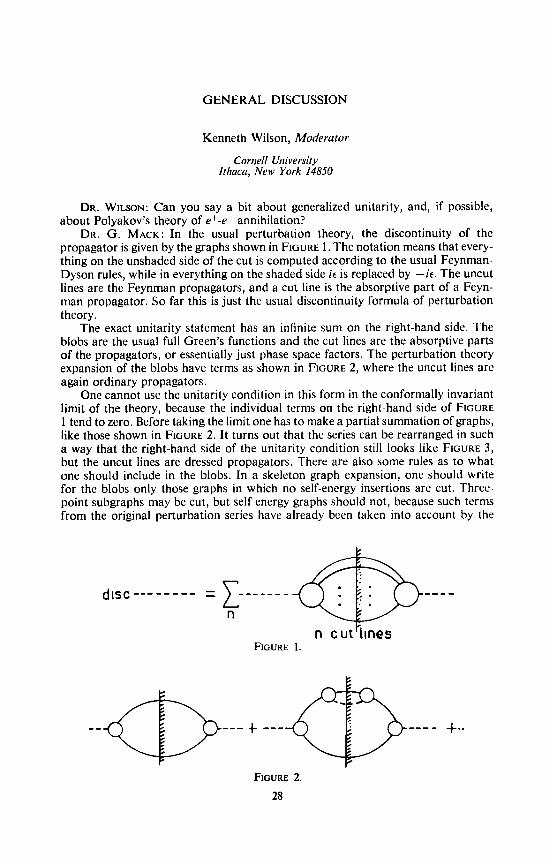
DR. G . MACK: In the usual perturbation theory, the discontinuity of the propagator is given by the graphs shown in FIGURE 1. The notation means that everything on the unshaded side of the cut is computed according to the usual Feynman- Dyson rules, while in everything on the shaded side k is replaced by -k. The uncut lines are the Feynman propagators, and a cut line is the absorptive part of a Feyn- man propagator. So far this is just the usual discontinuity formula of perturbation theory.

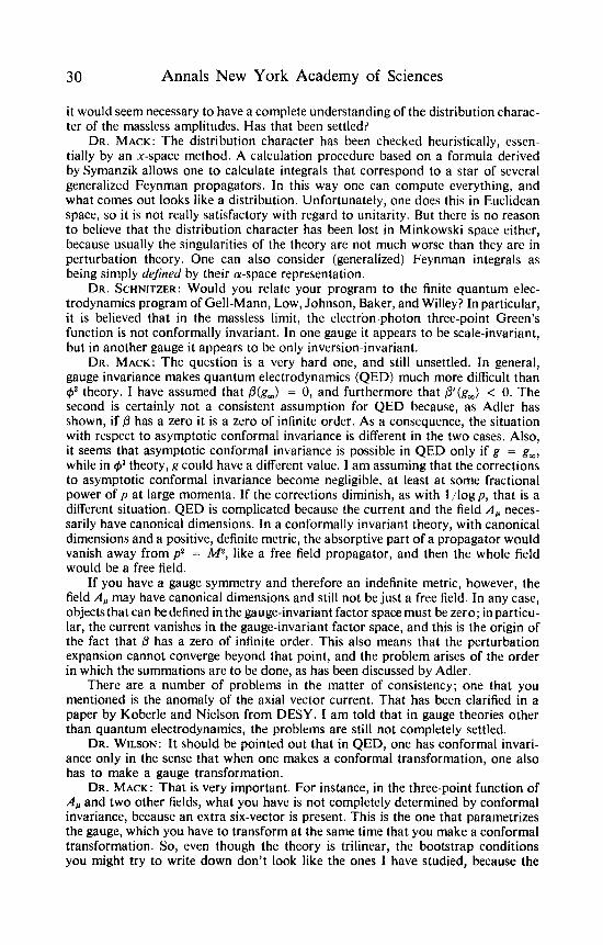
The exact unitarity statement has an infinite sum on the right-hand side. The blobs are the usual full Green’s functions and the cut lines are the absorptive parts of the propagators, or essentially just phase space factors. The perturbation theory expansion of the blobs have terms as shown in FIGURE 2, where the uncut lines are again ordinary propagators.

One cannot use the unitarity condition in this form in the conformally invariant limit of the theory, because the individual terms on the right-hand side of FIGURE 1 tend to zero. Before taking the limit one has to make a partial summation of graphs, like those shown in FIGURE 2. It turns out that the series can be rearranged in such a way that the right-hand side of the unitarity condition still looks like FIGURE 3, but the uncut lines are dressed propagators. There are also some rules as to what one should include in the blobs. In a skeleton graph expansion, one should write for the blobs only those graphs in which no self-energy insertions are cut. Three- point subgraphs may be cut, but self-energy graphs should not, because such terms from the original perturbation series have already been taken into account by the

FIGURE 2. 28

General Discussion 29

n cut‘bnes FIGURE 3

partial summation. This is the type of unitarity Polyakov used, but it was invented earlier, possibly first by Veltman.

Unitarity in this form makes sense for the conformally invariant theory, because the individual terms on the right-hand side of FIGURE 3 have a finite limit, and one can check that a t least the right-hand side is dilatation-invariant. It has also been checked that unitarity is satisfied in the skeleton graph expansion, as a consequence of the validity of the integral equations for the propagator and vertex boot strap; this was checked by Symanzik and myself.

This i‘s about as much as 1 know. The application to physical processes in which finite masses come into play, as in the Polyakov theory of e+-e- annihilation, I’m not prepared to discuss.

DR. P. K . MITTER (University of’ Marylund, College Park, Maryland): Since your limit theory is massless, it is not sufficient merely t o establish the ultraviolet convergence of the Feynman graphs. Have you checked on the infrared conver- gences, and d o you not expect that the analytical formula you wrote down in terms of the dimensions will change due t o the presence of actual massless particles in the theory?

DR. MACK: The infrared convergence of the theory has been checked. There is no problem. So long as we are away from the mass shells in which p2 = 0 (or, if we are in the Euclidean region, so long as we are away from the so-called exceptional momenta, which are those at which some nontrivial partial sum of the external momenta vanish) then the Green’s functions exist. There is a simple argument (created by Adler) to support this: In the six-dimensional formulation, the elements of the space are the rays on the light cone, and it turns out that this is in fact a compact space. Actually, one has to use the Euclidean quantum field theory, because only then is it possible to have a global conformal invariance. The cone is then of the usual light-cone type, with five pluses and one minus. (One needs only the positive cone, which is a well-defined object). Now, because it is sufficient t o know things as a function of rays on the cone, we can consider the cone as a projective space, and this is just a five-sphere, which is compact. (The essential point, of course, is the topology, and its invariance under a group.) In any case, in a compact space there is no such thing as a large distance.

The infrared divergences of the catastrophic kind (those that d o not just give singularities a t certain momenta, but ruin even the existence of Green’s functions) can come only from the divergence of integrals a t large values of x. But since essentially there are no large values of x, nothing catastrophic can happen.

The “ultraviolet” singular surfaces are defined by -Ca = I$D-integer. In general, there are additional singular surfaces in a massless theory. Even if they exist, it is easy to show they do not go through the neighborhood. 1 was considering the cases D = 6 and d = 2. In fact, according to Adler’s argument, they don’t exist in a conformally invariant theory.

DR. MITTER: 1 have another question. In writing down these unitarity equations,

30 Annals New York Academy of Sciences

it would seem necessary to have a complete understanding of the distribution character of the massless amplitudes. Has that been settled?

DR. MACK: The distribution character has been checked heuristically, essentially by a n x-space method. A calculation procedure based on a formula derived by Symanzik allows one t o calculate integrals that correspond to a star of several generalized Feynman propagators. In this way one can compute everything, and what comes out looks like a distribution. Unfortunately, one does this in Euclidean space, so it is not really satisfactory with regard t o unitarity. But there is no reason t o believe that the distribution character has been lost in Minkowski space either, because usually the singularities of the theory are not much worse than they are in perturbation theory. One can also consider (generalized) Feynman integrals as being simply defined by their a-space representation.

DR. SCHNITZER: Would you relate your program to the finite quantum electrodynamics program of Gell-Mann, Low, Johnson, Baker, and Willey? In particular, it is believed that in the massless limit, the electron-photon three-point Green’s function is not conformally invariant. In one gauge it appears to be scale-invariant, but in another gauge it appears t o be only inversion-invariant.

DR. MACK: The question is a very hard one, and still unsettled. In general, gauge invariance makes quantum electrodynamics (QED) much more difficult than c#+ theory. I have assumed that p(g-4,) = 0, and furthermore that p’(g,) < 0. The second is certainly not a consistent assumption for QED because, as Adler has shown, if 0 has a zero it is a zero of infinite order. As a consequence, the situation with respect to asymptotic conformal invariance is diKerent in the two cases. Also, it seems that asymptotic conformal invariance is possible in Q E D only if g = g,, while in c#9 theory, g could have a different value. I a m assuming that the corrections to asymptotic conformal invariance become negligible, a t least a t some fractional power of p a t large momenta. If the corrections diminish, as with 1 /logp, that is a different situation. QED is complicated because the current and the field A, neces- sarily have canonical dimensions. In a conformally invariant theory, with canonical dimensions and a positive, definite metric, the absorptive part of a propagator would vanish away from p 2 = M2, like a free field propagator, and then the whole field would be a free field.

If you have a gauge symmetry and therefore an indefinite metric, however, the field A, may have canonical dimensions and still not be just a free field. In any case, objectsthat can bedefined in the gauge-invariant factor space must be zero; in particular, the current vanishes in the gauge-invariant factor space, and this is the origin of the fact that fi has a zero of infinite order. This also means that the perturbation expansion cannot converge beyond that point, and the problem arises of the order in which the summations are to be done, as has been discussed by Adler.

There are a number of problems in the matter of consistency; one that you mentioned is the anomaly of the axial vector current. That has been clarified in a paper by Koberle and Nielson from DESY. I am told that in gauge theories other than quantum electrodynamics, the problems are still not completely settled.

DR. WILSON: It should be pointed out that in QED, one has conformal invariance only in the sense that when one makes a conformal transformation, one also has to make a gauge transformation.

DR. MACK: That is very important. For instance, in the three-point function of A, and two other fields, what you have is not completely determined by conformal invariance, because an extra six-vector is present. This is the one that parametrizes the gauge, which you have to transform at the same time that you make a conformal transformation. So, even though the theory is trilinear, the bootstrap conditions you might try to write down don’t look like the ones I have studied, because the


three-point function isn't determined by conformal invariance alone. Englert has tried to work on the bootstrap problem for QED.

DR. J . D. BJORKEN: I just want to make a small point about the measurability of the $-dependence of the momenta. Even if the present data were known with infinite accuracy, there would still be a problem, because one doesn't know whether to use w , w', w (Weitzman), or other parameters in computing those moments from experimental data. In the present q2 range, the variation in the y2-dependence that one gets on changing from w t o w' might just amount t o a stronger q2-dependence than the one that can be computed theoretically.

DR. MACK: That is troublesome, of course. It is a question of how fast the limit will be approached, and what is the best variable to use in order that the approach be fastest. You never know whether you are really in asymptopia, so you don't know how meaningful you can take your data to be. I don't know what the National Accelerator Laboratory will tell us when they get a Muon beam, but I hope the question will not be so crucial then.

DR. J . SULLIVAN: Is all of what you have said compatible with current algebra as we know it, from the point of view of the usual canonical field theory considera- tions?

DR. MACK: The minimal requirement, namely, that charges should commute correctly with the currents, is fulfilled. That follows from the Ward identities for the special case of two currents, and the Ward identities have been checked for SU, x SU,, or whatever symmetry you want. Whether you can commute space components of currents is another matter. I think it should be possible, but the coefficients might be anomalous.

DR. WILSON: Could you say something about the bootstrap in 3.99 dimensions for 44 theory, and about the way that Migdal and Polyakov propose to deal with it?

DR. MACK: The first trick is to introduce 4' as an independent field, and to work out the graphical rules for the new (dotted) line in canonical perturbation theory (FIGURE 4). The elementary quadrilinear vertex g44 is replaced by the sum of three terms, each of the form dg+q5(q5'---- d&~~)(pq5 (FIGURE 4a). The bare propagator of the new line (----) is just i , and the dressed propagator for the q5' field is developed in the usual way as a dotted line plus a series that consists of terms with dotted and solid lines joined at trilinear vertices dgq5q5qP (FIGURE 4b). There are also tadpoles, but they don't survive in the conformal invariant limit. In this way one can rearrange the Feynman series into a form that looks like the Feynman series for a trilinear coupling, except that there are now two types of line and the propagator for the dashed line is just i. One can then also write down skeleton graph expansions.


Since the theory is trilinear, one can go to 3.99 dimensions and write bootstrap equations similar to the ones shown before, except that there are two types of line. There are additional bootstrap conditions for the extra field +*.

The thorny part of the problem comes when one tries t o expand using the equation t = 4 - D. I t is no longer true that the first term in the skeleton graph expansion is the only one that is of the order t. There are an infinite number of them. They originate from the following problem: In +s theory, by going over t o the dressed three-point function and dressed propagator, one has absorbed all the renormaliza- tion parts. There are no divergences left in D = 6 dimensions, so that if one goes to the canonical limit one gets a convergent Feynman diagram. That is not true for 44 theory in (4 - t) dimensions, because in this case one has not correctly absorbed the box diagram divergences. Graphs with four external legs are convergent so long as one is in 3.99 dimensions, but they become divergent when one goes to 4 dimensions, and that gives a n extra factor of l / e . Unfortunately, it turns out that there are so many such terms that they kill the factors of t that come from the coupling constants. Hence there is a n infinite series t o sum, even of the order t.

DR. WILSON: Will this same difficulty arise in Yukawa theory? DR. MACK: No. In Yukawa theory there are box graphs, but not enough of

them to compensate for the t-factors from the coupling constant. DR. MITTER: If you d o not make the t-expansion in these bootstrap theories, is

the final problem of solving the bootstrap any simpler than solving the Gell-Mann- Low eigenvalue condition?

DR. MACK: If one is optimistic, one can simply assume that the leading graph is already a good approximation of the solution of the bootstrap. Fradkin has adopted this attitude, and he told me that he got a value for d,, of 1.8, instead of the canonical value of 1.5. He claims there is a solution for y5 theory too. The problem of the convergence of the series is an important one, however.

There are essentially two methods that are not based on such optimism. The first is related to the €-expansion. You cannot hope that va will ever give the theory of the real world, but just to explain the idea, I shall plot the trajectories of theory in the ( D , d ) plane as a function of g (FIGURE 5 ) . As the small g a t, we have the germ of a solution near the point (6,2).

FIGURE 5.


Now, we can put bounds on the trajectory for larger values of g . I have not explained it in detail, but the left-hand side of the propagator bootstrap equation vanishes when d = ‘50 - 1 + an integer, while the left-hand side of the vertex bootstrap equation vanishes along another set of straight lines. Moreover, the right- hand sides are always finite; this is basically the reason why we can find a solution. We can expand about a point where two lines cross. On the other hand, the solution can never cross one of the lines just mentioned, because there the right-hand side of the equation is zero and the left side is not. The solution manifold therefore has t o lie inside certain strips, except that it can pass through the intersections of different lines; at such points g = 0.

The idea is that somehow the solutions manifold must connect t o form global surfaces. From the germ at ( 6 , 2 ) , the solution either goes up through (8,4) or turns around and comes down through (4 , l ) . You can try to argue, for instance, that if it goes up it should pass through D = 7, and there should be a solution with anomalous dimensions at D = 7. There is no very good way of computing it, but you may be able to d o something. On the other hand, if you have bad luck, it turns down and passes through D = 4. Anyway, 41~ theory is not a very realistic model. Maybe it works for some other model. It is a method that one can use in place of a possible nonconvergent approximation scheme. Long ago one has been forced to go from quantitative t o qualitative arguments in classical mechanics. Maybe we have t o d o the same thing here.

The other method is t o try t o construct the theory in a n entirely different way, not using skeleton graph expansions at all, but instead trying to solve the integral equations directly by a group theoretical approach. I’ve started to work on this and I have some results which I hope will lead to some progress. (Mack, G. 1973. Group theoretical approach t o conformal invariant QFT. Bern preprint.)

DR. WILSON: As a n application of the conformally invariant bootstrap, I’d like t o say something about Polyakov’s theory of e+-e- annihilation. Let’s say you want to understand the multiplicity of hadrons in e+-e- annihilation. It is very hard to do that directly from a conformally invariant picture, because the amplitudes at which the particles are actually produced are not, of course, conformally invariant, even a t a very high center of mass energies. The particles are still on the mass shell. Now, Dr. Mack Ms already explained that within a bootstrap theory one can de- velop another version of unitarity, in which instead of having particles on the mass shell, one has absorptive parts of propagators, and the absorptive part of a propagator exists for all mass square, not just on the mass shell.

Polyakov uses the generalized unitarity to write an expression for the absorptive part of the current propagator (FIGURE 6). That means that the blobs are amplitudes for a current that is going into actual fields, not just particles, and the cut lines that join the two blobs are absorptive parts of the propagators. You sum over the number of lines that go across. The point is that if you take one term of the sum, with a fixed number of lines going across, this term is by itself conformally invariant and scale-invariant, with the same scale invariance as the original graph. Therefore you can postulate that when summing up these graphs, you need take only a finite number of terms, up t o a finite number of lines going across, to achieve a given accuracy. This does not have to be the case, but Polyakov assumed that you can restrict the sum in practice. If there were ordinary particles going across, you would certainly expect to have to d o a n infinite sum.

Making Polyakov’s assumption, you get the following picture: Let’s take the simplest possibility and imagine that the dominant term is the one with just two lines going across. Each cut line is itself the absorptive part of a propagator, so one can use unitarity t o break it down into two blobs joined by cut lines and again


FIGURE 6.

imagine that the dominant term has just two lines going across. There are now four cut lines, and each of them is the absorptive part of a propagator, so you can break it down further. Now, you know what happens. A certain center of mass energy is coming in at the left, and it has to split up between the two internal lines at the first level. Each internal line carries less energy than the external line, and you expect that each line at the first level carries maybe half of the original energy. At the second level each line goes down to about a quarter of the original energy. You can repeat the process, but if you started with finite s (where s is the square of the center of mass energy going in), then after a certain number of iterations you will wind down to the point where the energy of each line is of the order of the mass of the particles, and then you can’t use conformal invariance any more. At that Qoint you stop, because effectively you will just get back to the mass shell of the particles. The number of steps you can take is logs. What remains in the end is just the real particles, because the energy is reduced to the point where the only thing on each line is a single real particle. This is Polyakov’s strange picture of how the particles are produced in e+-e- annihilation.

You can see, if you make this simple-minded assumption that there are just two lines each time, that the final multiplicity is proportional to a power of s; this is because there are logs levels and the number of particles is doubled each time. Polyakov is unable to tell you what the power is; he just says it is some power. I’m giving this discussion because I want somebody to look at it in detail in one of these models, such as those Dr. Mack has discussed, to find out what is really going on and whether the picture is right, and if so to determine some of the parameters that Polyakov can’t calculate, such as the power.

DR. BJORKEN: Aside from the multiplicity, what can be said about the total cross-section? Is the s-dependence anomalous?

DR. WILSON: The total cross-section just depends on the dimensions of the current, so it must be normal. Polyakov says that too. It is just scale invariance. It is only in questions such as multiplicity, which one can’t get from scale invariance alone, that one uses Polyakov’s idea. Another very interesting feature of the model


is the following: At the first vertex everything is scale-invariant, and we imagine that along with scale invariance there are complete S U , or S U , x SU3 invariances. This suggests that it is reasonably likely that lines a t the first level carry strangeness. If they don’t produce strangeness a t the first vertex, there is still a reasonable prob- ability that they will produce it a t the second, because they are still a t rather high energies and in the SU,-invariant region. But once one of the lines acquires strangeness, there is no place that the strangeness can be annihilated, because of the branch- ing structure. If strangeness appears a t any of the vertices, it is going to come out in the final state as an actual particle with strangeness. That means that by the time there is a large number of particles, the chance of getting a K particle is enormous. Furthermore, unless there is a strange Clebsh-Gordon coefficient in the initial stages, you would expect to see many K’s and T ’ S , probably an equal number of them. It is hard to discuss the ratio of K’s to A’S, because that is determined in the final stages, where there is no longer any SU,.

This is the same sort of argument as I gave (but with much less substance behind it) to show that there ought to be lots of K’s in deep inelastic scattering. Unfortu- nately, no evidence has been found for it yet.

general discussion

Documents