CHAPTER 1

General Introduction

(

1.1 Ships

The Earth may be regarded as a "water planet" , since 71 percent of its sur­face is covered by water having an average depth of 3.7 km. Transportation across the oceans must therefore have engaged the. attention of humankind since the dawn of history. Ships started thousands of years ago as si~ple logs or bundles of reeds and have deve19ped into the huge complicated ves­sels of today. \"ooden sailing ships are known to have appeared by about 1500 BC and had developed into vessels sailing around the world by about 1500 AD. Mechanical propulsion began to be used in ships by the beginning of the 19th Century, and iron followed by steel gradually took the place of wood for building large oceangoing ships, with the first iron-hulled ship, the "Great Britain", being launched in 1840.

Ships today can be characterised in several ways. From the point of view of propulsion, ships may be either self-propelled or non-propelled requiring external assistance to move from one point to another. Ships may be ocean­going or operating in coastal waters or inland waterways. Merchant ships which engage in trade are of many different kinds such as tankers, bulk carri­ers, dry cargo ships, container vessels and passenger ships. Warships may be divided into ships that operate on the surface of water such as frigates and aircraft carriers, and ships that are capable of operating under water, viz. submarines. There are also vessels that provide auxiliary services such as tugs and dredgers. Fishing vessels constitute another important ship type.

1

L

i

I J

2 Basic Ship Propulsion

Most of these types of ships have very similar propulsion arrangements. Hm\'ever, there are some types of very high speed vessels such as hovercraft and hydrofoil craft that make use of unconventional propulsion systems.

1. 2 Propulsion Machinery I For centuries, ships were propelled either by human power (e.g. by oars) or by ''lind power (sails). The development of the steam engine in the 18th Century' led to attempts at using this new source of power for ship propulsion, and the first steam driven ship began operation in Scotland in 1801. The early steam engines were of the reciprocating type. Steam was produced in! a boiler from raw sea water using wood or coal as fuel. Gradual advances in steam propulsion plants took place during the 19th Century, including the use of fresh water instead of sea water and oil instead of coal, improvements in boilers, the use of condensers and the development of compound steam engines. Reciprocating steam engines were' widely used for ship propulsion

It

,f f

till the early years of the 20th Century, but have since then been gradually superseded by steam turbines and diesel engines. '

The first marine steam turbine was fitted in the vessel "'I'urbinia"in 1894 by Sir Charles Parsons. Since then, steam turbines have completely replaced

J I

I reciprocating steam engines in steam ships. Steam turbines produce less vibration than reciprocating engines, make more efficient use of the high steam inlet pressures and very low exhaust pressures available with modern steam ge,nerating and condensing equipment, and can be designed to produce very high powers. On the other hand, turbines run at very high speeds and cannot be directly connected to ship propellers; nor can turbines be reversed. This makes it necessary to adopt special arrangements for speed reduction and reversing, the usual arrangements being mechanical speed reduction

1 I

\IIj

Ij

! gearing and a special astern turbine stage, or a turbo-electric drive. These i

\ arrangements add to the cost and complexity of the propulsion plant and .~

I,also reduce its efficiency.t ~

Since its invention in 1892, the diesel engine has continued to grow in popularity for usc in ship propulsion and is today the most common type of engine used in ships. Diesel engines come in a wide range of powers ~nd

I

. \

! '

t speeds, arc capable of using low grade fuels, and are comparatively efficient.

. t

-----------~

General Introduction 3

Low speed diesel engines can be directly connected to ship propellers and can be reversed to allow the ship to move astern.

Another type of engine used for ship propulsion is the gas turbine. Like the steam turbine, the gas turbine runs at a very high speed and cannot be reversed. Gas turbines are mostly used in high speed ships where their low weight and volume for a given power give them a great advantage over"other types of engines.

Nuclear energy has been tried for ship propulsion. The heat generated by a nuclear reaction is used to produce steam to drive propulsion turbines. However, the dangers of nuclear radiation in case of an accident have pre­vented nuclear ship propulsion from being used in non-combatant vessels exc~pt for a few experimental ships such as the American- ship "Savannah", the German freighter "Otto Hahn"and the Russian icebreaker "V.l. Lenin". Nuclear propulsion has been used in large submarines with great success because nuclear fuel contains a large amount of energy in a very small mass, and because no oxygen is required for gen~rating heat. This enables a nu­clear submarine to travel long distances under water, unlike a conventional submarine which has to come to the surface frequently to replenish fuel and air for combustion.

In addition to the conventional types of ship propulsion plant discussed in the foregoing, attempts are being made to harness renewable and non­polluting energy sources such as solar energy, wind energy and wave energy for ship propulsion and to develop advanced technologies such as supercon­ductivity and magneto-hydrodynamics. However, these attempts are still in a preliminary experimental stage.

1.3 Propulsion Devices

Until the advent of the steam engine, ships were largely propelled by oars imparting momentum to the surrounding water or by sails capturing the energy of the wind. The first mechanical propulsion device to be widely used in ships was the paddle wheel, consisting of a wheel rotating about a transverse axis with radial plates or paddles to impart an astern momentum to the water around the ship giving it a forward thrust. The early steam­ers of the 19th Century were all propelled by paddle wheels. Paddle wheels

4 Basic Ship Propulsion

are quite efficient when compared with other propulsion devices but have several drawbacks including difficulties caused by the variable immersion of the paddle wheel in the different loading conditions of the ship, the increase in the overall breadth of the ship fitted with side paddle wheels, the inabil­ity of the ship to maintain a steady course when rolling and the need for slow running heavy machinery for driving the paddle wheels. Paddle wheels were therefore gradually superseded by screw propellers for the propulsion of oceangoing ships during the latter half of the 19th Century.

The Archimedean screw. had been used to pump water for centuries, -and proposals had been made to adapt it for ship propulsion by using it to impart momentum to the water at the stern of a ship. The first actual use of a screw to propel a ship appears to have b~en made in 1804 by the American, Colonel Stevens. In 1828, Josef Ressel of Trieste successfully used a screw propeller in an 18 m long experimental steamship. The first practical applications of screw propellers were made in 1836 by Ericsson in America and Petit Smith in England. Petit Smith's propeller consisted of a wooden screw of one thread and two complete turns. During trials, an accident caused a part of the propeller to break off and this surprisingly led to an incr~8.se in the speed of the ship. Petit Smith then improved the design of his propeller by decreasing the width of the blades and increasing the number of threads, producing a screw very similar to modern marine propellers. The screw propeller has since then become the predominant propulsion device used in shipl3.

Certain variants of the screw propeller are used for special applications. One such variant is to enclose the propeller in a shroud or nozzle. This improves the performance of heavily loaded propellers, such as those used in tugs. A controllable pitch propeller allows the propeller loading to be varied over a wide range without changing the speed of revolution of the propeller. It is also possible to reverse the direction of propeller thrust without chang­ing the direction of revolution. This allows one to use non-reversing engines such as gas turbines. When propeller diameters are restricted and the pro­pellers are required to produce large thrusts, as is the case in certain very high speed vessels, the propellers are likely to experience a phenomenon called "cavitation", which is discussed in Chapter 6. In cjrcumstances where extensive cavitation is unavoidable, t.he propellers are specially designed to

L

5 General Introduction

operate in conditions of full cavitation. Such propellers are popularly known as "supercavitating propellers".

Problems due to conditions of high propeller thrust and restricted diame­ter, which might lead to harmful cavitation and reduced efficiency, may be avoided by dividing the load between two propellers on the same shaft. Mul­tiple propellers mounted on a single shaft and turning in the same direction are called "tandem propellers". Some improvement in efficiency can be 0 b­tained by having the two propellers rotate in opposite directions on coaxial shafts; Such "contra-rotating propellers"are widely used in torpedoes.

I

Two other ship propulsion devices may be IIl;entioned here. One is the vertical axis cycloidal propeller, which consists 6f a horizontal disc carrying a number of vertical blades projecting below W.As the disc rotates about a vertical· axis, each blade is constrained to t.urn about its own axis such that all the blades produce thrusts in the same direction. This direction can be controlled by a mechanism for setting the positions of the vertical blades. The vertical axis propeller can thus produce a thrust in any direction, ahead, astern or sideways, thereby greatly/improving the manoeuvrability of the vessel. The second propulsion device that may be mentioned is the waterjet. Historically, this is said to be the oldest mechanical ship propulsion device, an English patent for it having been granted to Toogood and Hayes in 1661. In waterjet propulsio~, as used today in high speed vessels, an impeller draws water from below the ship and discharges it astern in a high velocity jet just above the surface of water. A device is provided by which the direction of the waterjet can be controlled and even reversed to give good manoeunability. Waterjet propulsion gives good efficiencies i1\ high speed craft and is becoming increasingly popular for such craft.

Because of their overwhelming importance in ship propulsion today, this book deals mainly with screw propellers. Other propulsion devices, including variants of the screw propeller, are discussed.in Chapter 12.

l,

__~

I . f

CHAPTER 2

Screw Propellers

2.1 Description

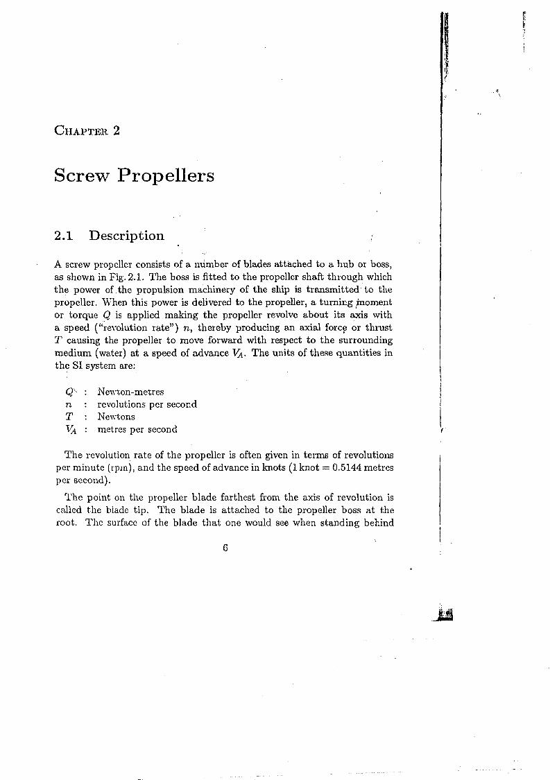
A screw propeller consists of a number of blades attached to a hub or boss, as shown in Fig. 2.1. The boss is fitted to the propeller shaft throughwhich the power of .the propulsion machinery of the ship is transmitted to the propeller. When this power is delivered to the propeller, a turning ,moment or torque Q is applied making the propeller revolve about its axis with a speed ("reyolution rate") n, thereby producing an axial forc~ or thrust T causing the propeller to move forward with respect to the surrounding

\

II\,II

I(

medium (water) at a speed of advance VA. The units of these quantities in the 81 system are:

Q" Newton-metres n revolutions per second T Newtons VA metres per second

The revolution rate of the propeller is often given in terms of revolutions per minute (rpm), and the speed of advance in knots (1 knot = 0.5144 metres per second).

The point on the propeller blade farthest from the axis of revolution is called the biade tip. The blade is attached to the propeller boss at the root. The surface of the blade that one would see when standing behind

6

7 Seren' Propellers

DIRECTION OF REVOLUTION FOR AHEAD MOTION

TIP

TRAILING EDGE .' ­

PROPELLER . SHAFT

...... --.,..,.,..

AXISL ..-'.-'.-'

PROPELLER

LEADING EDGE

Figure 2.1 : A Three-Bladed Right Hand Propeller.

the ship and looking at the propeller fitted at the stern is called the face of the propeller blade. The opposite surface of the blade is called its back. A propeller that revolves in the clockwise direction (viewed from aft) when propelling the ship forward is called a right hand propeller. If the propeller turns anticlockwise when driving the ship ahead, the propeller is left handed. The edge of the propeller blade which leads the blade in its revolution when the ship is being driven forward is called the leading edge. The other edge is the trailing edge.

(

'When a propeller revolves about its axis, its blade tips trace out a circle. The diameter of this circle is the propeller diameter D. .The number of p~opeller blades is denoted by Z. The face of the propeller blade either forms a part of a helicoidal or ss;rew ~urface, or is defined with respect to it; hence the name "screw propeller". A h'~iicoidal surface is generated when a line revolves about an axis while simultaneously advancing along it. A point on the line generates a three-dimensional curve called a helix. The distance that the line (or a point on it) advances along the axis in one revolution is called the pitch of the helicoidal surface (or the helix). The pitch of the

8 Basic Ship Propulsion

RAKE ANGLE E

I !

NO RAKE RAKE AFT i

. i (0) RAKE

, }

NO MODERATELY SKEW SKEINED

(b) SKEW

Figure 2.2 : Raile and Silew. \.

helicoidal surface which defines the face of a propeller blade is called the . ,(face) pitch P of the propeller. !

If the line generating the helicoidal surface is perpendicular to the axis about which it rotates when advancing along it, the helicoidal surface and the propeller blade defined by it are said to have no rake. If, however, the generating line is inclined by an angle e to the normal, then the propeller has a rake angle e. The axial distance betwe~n points on the generating

.,line at the blade tip and at the propeller axis is the rake. Propeller blades , are sometimes raked aft at angles up to 15 degrees to increase the clearance (space) between the propeller blades and the hull of the ship, Fig. 2.2(a). '

HEAVILY SKEWED

Screw Propellers 9

Com-:ider the line obtained by joining the midpoints between the leading and trailing edges of a blade at different radii from the axis. If this line is straight and passes through the axis of the propeller, the propeller blades have no skew. Usually ho~ever, the line joining the midpoints curves towards the trailing edge, resulting in a propeller whose blades are skewed back. ~kew..

i,s~d to reduce vibration. Some modern propeller designs have heavily skewed blades. The angle Os between a straight line joining the centre of

\

the propeller tq .iha..midRQinL~~JheWt and a line joining the centre and the midpoint at the blade tip is a measure of skew, Fig.2.2(b)..

Example 1

In a propeller of 4.0 m diameter and 3.0 m constant pitch, each blade face coincides with its defining helicoidal surface. The distance. of the blade'tip face from a plane normal to the axis is 263.3 mm, while the distance of a point on the face at the root section (radius 400 mm) from the same plane is .52.7 mm, both distances being measured in a plane through. the propeller axis: The midpoint of-the root section is 69.5'mm towards the leading edge from a plane through the propeller axis, while the blade tip is 1:285.6 mm towards the trailing ~dge from the same plane. Determine the rake and skew angles of thepropell~

The tangent of the rake angle is given by:

difference in rake of the two sections 263.3 - 52.7tan£; = =

difference in their radii 2000 - 400

= 0.131625

Rake angle € = 7.5 0

The angles which the midpoints of the root section and the tip make with the reference plane are given by:

sineo = 69.5 = 0.17375 eo = 10.000

400

-1285.6 sin e1 = = -0.64280

2000

The skew angle is therefore (eo - ( 1 ) = 500

4

10 Basic Ship Propulsion

2.2 Propeller Geometry

The shape of the blades of a propeller is usually defined by specifying the shapes of sections obtained by the intersection of a blade by coaxial right circular cylinders of different radii. These sections are called radial sections or cylindrical sections. Since all the Z propeller blades are identical, only one blade needs to be defined. It is convenient to use cylindrical polar coordinates (r, e, z) to define any point on the propeller, r being the radius measured from the propeller a.xis, ean angle measured from a reference plane passiI).g through the axis, and z the distance from another reference plane normal to the axis. The z = 0 reference plane is usually taken to pass through the intersection of the propeller axis and the generating line of the helicoidal surface in the e= 0 plane. !

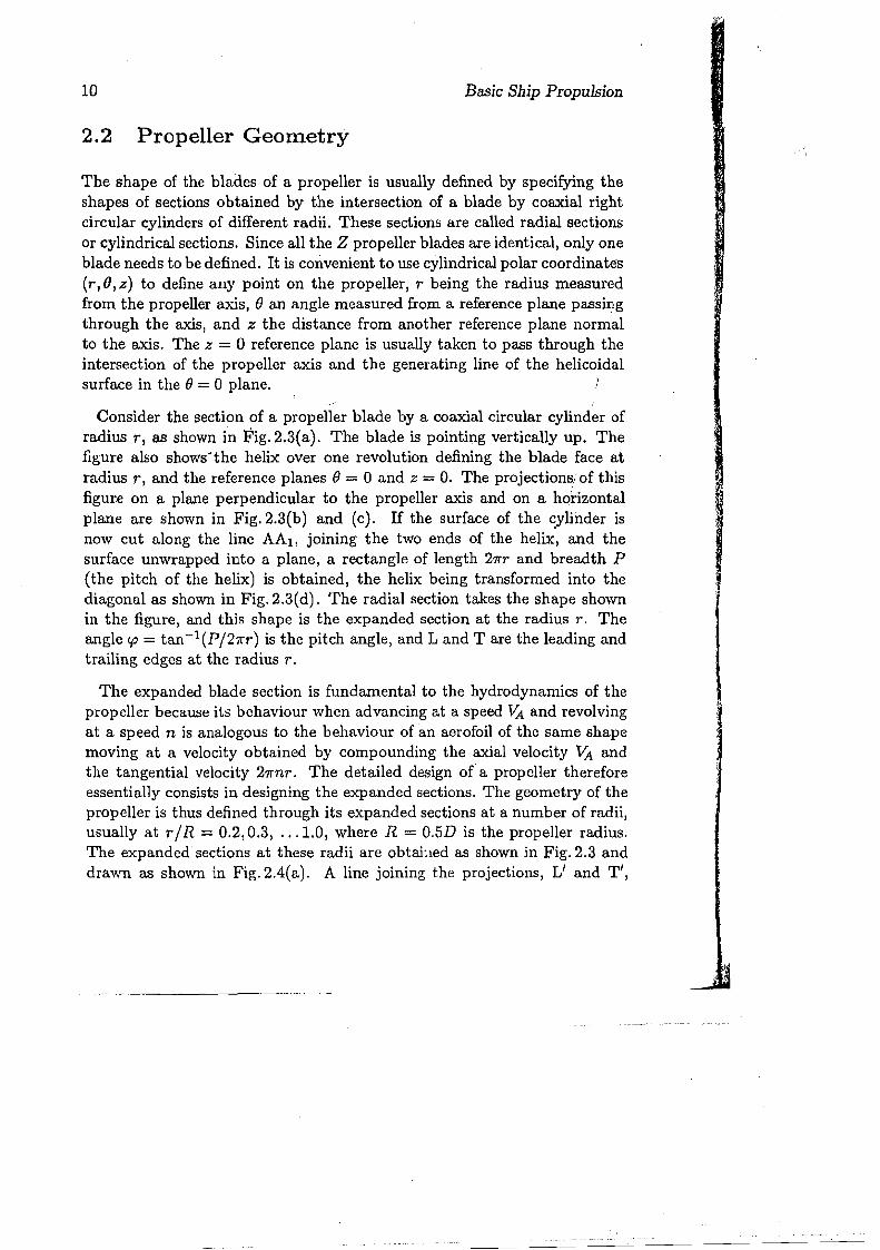
., , Consider the section of a propeller blade by a coaxial circular cylinder of

radius r, as shown in Fig.2.3(a). The blade is pointing vertically up. The figure also shows~the helix over one revolution defining the blade face at radius r, and the reference planes e= 0 and z = O. The projections; of this figure on a plane perpendicular to the propeller axis and on a hqrizontal plane are shown in Fig. 2.3(b) and (c). If the surface of the c:ylirider is now cut along the line AAl, joining the two ends of the helix, and the surface unwrapped into a plane, a rectangle of length 27rr and breadth P (the pitch of the helix) is obtained, the helix being transformed into the diagonal as shown in Fig. 2.3(d). The radial section takes the shape shown in the figure, and this shape is the expanded section at the radius r. The angle <p = tan-1(P/27rr) is the pitch angle, and Land T are the leading and trailing edges at the radius r.

The expanded blade section is fundamental to the hydrodynamics of the propeller because its behaviour when advancing at a speed l'A. and revolving at a speed n is analogous to the behaviour of an aerofoil of the same shape moving at a velocity obtained by compounding the axial velocity "A and the tangential velocity 27rnr. The detailed design of a propeller therefore essentially consists in designing the expanded sections. The geometry of the propeller is thus defined through its expanded sections at a number of radii, usually at r / R = 0.2,0.3, " .1.0, where R = 0.5D is the propeller radius. The expanded sections at these radii are obtai:led as shown in Fig. 2.3 and drawn as shown in Fig.2.4(a). A line joining the projections, L' and Ti,

11 Screw Propellers

of the leading and trailing edges on the base line of each section gives the expanded blade outline. The area within the expanded outlines of all the blades is the expanded blade area, AE.

HELIX (0)

A

(b)

CYLINDER. RADIUS r

(d) (c) z

1r pp

L 1A~¢L--------I

1---2TIr----!

t

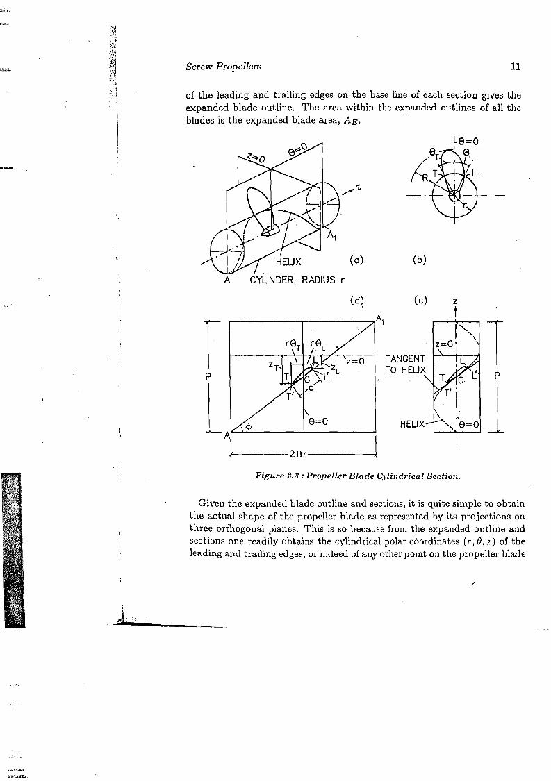
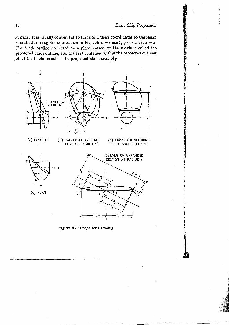
Figure 2.3: Propeller Blade Cylindrical Section.

Given the expanded blade outline and sections, it is quite simple to obtain the actual shape of the propeller blade as represented by its projections on three orthogonal planes. This is so because from the expanded outline and sections one readily obtains the cylindrical polar coordinates (r, (), z) of the leading and trailing edges, or indeed of any other point on the propeller blade

12 Basic Ship Propulsion

surface. It is usually convenient to transform these coordinates to Cartesian coordinates using the axes shown in Fig. 2.4: x = r cos (), y = r sin (), z = z. The blade outline projected on a plane normal to the z-axis is called the projected blade outline, and the area contained within the projected outlines of all the blades is called the projected blade area, Ap.

IC x

+

p . m-t

(c) PROALE (b) PROJECTED OUTLINE (0) EXPANDED SECTIONS DEVELOPED OUTUNE EXPANDED OUTUNE

T . __ z

y

(d) PLAN

DETAILS OF EXPANDED SECTION AT RADIUS r

Figure 2.4 : Propeller Drawing.

13

L

Screw Propellers

The projections of the leading and trailing edges of a blade section on a plane tangential to the helix at the point C in Fig.2.3(d), Le. L' and T', are also associated '.'lith what is called the developed blade outline. If these tangent planes for the different radial sections are rotated through the pitch angles <p about the point C, the line joining the projections of the leading and trailing edges at the different radii gives the developed blade outline. The intersection of the tangent plane to the helix with th~ circular cylinder of radius r is an ellipse of semi-major axis rsec<p and semi-minor axis r. There­fore. in order to obtain the points on the developed outline corresponding to L' and T', it is necessary to draw this ellipse and to move the points L' and T' horizontally to L" and T" on the ellipse, Fig. 2.4(b). Alternatively, L" and T" may be obtained by measuring off d,istances equal to CL' and cT' in Fig.2.4(a) on the circumference of the ellipse as CL" 'and CT" respectively in Fig.2.4(b). Since drawing an ellipse m~nually is somewhat tedious, it is usual to approximate the ellipse by a circle having the same radius of cur­vature as the ellipse at the point C, Le. r sec2 <.p. The centre 0" of this circle may be obtained by the construction shown in Fig. 2.4(b). Paradoxically, the approximation of the ellipse by this circle gives more accurate results because the radius of the circle is exactly equal to the radius of curvature of the helix, which is constant. The developed outline represents what would be obtained if the curved surface of a propeller blade could be developed into a plane. The developed blade outline is sometimes of use during the manu­facture of a propeller. The area contained within the developed outlines of all the blades is called the developed blade area, AD.

A typical propeller drawing consists of the expanded outline and blade sections, the developed outline and the projections of the blade outline on the three orthogonal planes, x = 0, y = °and z = 0, as shown in Fig. 2.4. Instead of the projection of the propeller blade on the x - z plane shown in Fig.2.4(c), the values of z for the leading and trailing edges are sometimes plotted as a function of r to obtain the blade sweep, Le. the space swept by the blade during its revolution. This is important for determining the clearances of the propeller blade from the hull and the rudder, particularly for heavily skewed blades. The construction lines are naturally not given in the drawing. There are instead a number of additional details. Detailed offsets of the expanded sections are provided. A line showing the variation of the position of maximum thickness with radius is drawn on the expanded outline, and sometimes the loci of the points at which the face of the propeller

14 Basic Ship Propulsion

blade departs from its base line at the different radii. The offset of the face above its base line is' variously called wash-back, wash-up, wash-away or setback, a negative offset (below the base line) being called wash-down. The offsets of the leading and trailing edges are called nose tilt and tail tilt. The distribution of pitch over the radius, if not constant, is shown separately. The variation of maximum blade thickness with radius r and the fillet radii where the blade joins the boss are also indicated. The internal details of the boss showing how it is fitted to the propeller shaft may also be given.

Example 2

In a propeller of 5.0 m diameter and 4.0 m pitch, radial lines from the leading and trailing edges of the section at 0.6R make angles of 42.2 and 28.1 degrees with the reference plane through the propeller iaxis. Determine the width of the expanded blade outline at 0.6R.

The radius of the section at 0.6R, r = 0.6x 2 5 = 1.5m = 1500mm .,

"'.

The pitch angle at this section is given by:

'p 4 tanlp = - = = 0.4244 cos lp = 0.9205

21ir 21i X 1.5

lp = 22.997°

Referring to Fig. 2.3,

8T = 28.10 (given)

The width of the expanded outline at 0.6R is:

c = 8L and 8T being in radians

so that, 1500 [42.2

0 + 28.10

]

57.3 c = 0.9205 = 1999.2 nun

This assumes t.hat the section is flat faced, i.e. Land T in Fig. 2.3(c) coincide with L' and T' respectively.

15 Screw Propellers

Example 3

The cylindrical polar coordinates (r, B, z) of the trailing edge of a flat faced propeller blade radial section are (1500 nun, -30°, -400 nun). If the pitch of the propeller is 3.0 m, and the expanded blade width is 2000 mm, determine the coordinates of the leading edge.

The leading and trailing edges of a radial section have the same radius, Le. r = 1500rnm.

The pitch angle is given by:

P 3000tan'P = - = = 0.3183

21fr' 21f x 1500

'P = 17.657° cos'P = 0.9529 sin'P = 0.3033

If the a coordinates of the leading and trailing edges are BL and BTl then the expanded blade width c is given by:

r((h - aT)' . c = --'-----'-,aee FIg. 2.3(c)

cos'P . ,

1500 [a£ - (-300 )!l57.3Le. 2000 = --~=-0-.-:'95::-2-9'--':'::':""--

or

Also, ZL = ZT + c sin 'P

= -400 + 2000 x 0.3033 = 206.6 nun

Le. the coordinates of the leading edge are (1500 rom, 42.80°, 206.6 mm).

2.3 Propeller Blade Sections

The expanded blade sections used in propeller blades may generally be di­vided into two types: segmental sections and aerofoil sections. Segmental sections are characterised by a flat face and a circular or parabolic back, the maximum thickness being at the midpoint between the leading and trailing edges, the edges being quite sharp, Fig.2.5(a). In aerofoil sections, the face

16 Basic Ship Propulsion

-~-

_ ~ _ ---l~:===_..L1~-".L- _<E.::---'O-=O".:_"-"---Jte.--_":::?>o::::-"-::.--_

(0) SEGMENTAL (b) AEROFOIL (c) LENTICULAR

SECTION SECTIONS SECTION"

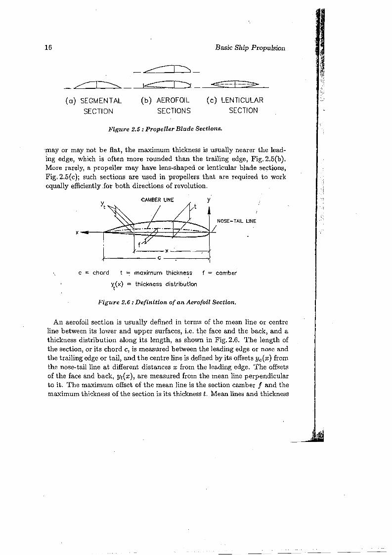
Figure 2.5: Propeller Blade Sections.

'mayor may not be flat, the maximum thickness is usually nearer the lead­ing edge, which is often more rounded than the trailing edge, Fig.2.5(b). More rarely, a propeller may have lens-shaped or lenticular blade sections, Fig.2.5(c)j such sections are used in propellers that are required to work equally efficiently for both direc'tions of revolution.

Yt CAMBER LINE

x"

NOSE-TAIL UNE:

X

i

~ C

\ C = chord t "7 maximum thickness f = comber

y (x) = thickness distribution t

Figure 2.6: Definition of an Aerofoil Section.

An aerofoil section is usually defined in terms of the mean line or centre line between its lower and upper surfaces, Le. the face and the back, and a thickness distribution along its length, as shown in Fig. 2.6. The length of the section, or its chord c, is measured between the leading edge or nose and the trailing edge or tail,and the centre line is defined by its offsets Yc(x) from the nose-tail line at different distances x from the leading edge. The offsets of the face and back, Yt(x), are measured from the mean line perpendicular to it. The maximum offset of the mean line is the section camber f and the maximum thickness of the section is its thickness t. Mean lines and thickness

17 Screw Propellers

distributions of some aerofoil sections used in marine propellers are given in Appendix 2.

Instead of measuring the section chord on the nose-tail line, it is usual in an expanded propeller blade section to define the chord as the projection of the nose-tail line on the base line, which corresponds to the helix at the given radius, i.e. the chord c is taken as L' T' rather than LT in Fig. 2.3(c) or Fig.2.4(a). If the resultant velocity of flow to a blade section is VR as shown in Fig.2.7, the angle between the base chord and the resultant velocity is

I

NO-L1FjT LINE

+

LIFT t DRAG

oI -.10

DRAG

Figure 2.7 : Angle ofAttack.

called the angle of attack, a. The blade section then produces a force whose components normal and parallel to VR are the lift and the drag respectively. For a given section shape, the lift and drag are functions of the angle of attack, and for a certain (negative) angle of attack the lift of the section is zero. This angle of attack is known as the 'no-lift angle, Qo.

2.4 Alternative Definition of Propeller Geometry

When a propeller is designed in detail beginning with the design of the expanded sections, the geometry of the propeller is sometimes defined in a slightly different way. The relative positions of the expanded sections are indicated in terms of a blade reference line, which is a curved line in space that passes through the midpoints of the nose-tail lines (chords) of the sections at the different radii. A cylindrical polar coordinate system (r,e,z) is chosen as shown in Fig. 2.8. The z = 0 reference plane is normal to the propeller axis, the e = 0 plane passes through the propeller axis (z-axis),

-:1... _

18 Basic Ship Propulsion

8=0 PLANE

z=o PLANE

z A

PITCH OF HELIX = P

SURFACE OF CYLINDER UNWRAPPED INTO A PLANE

z=o

8=0

p

A t'--------- 2 n r ----------.t Figure 2.8 : Alternative Definition of Propeller Geometry.

Screw Propellers 19

and both pass through the blade reference line at the boss. The pitch helix at any radius r passes through the 0 = 0 plane at that radius. The angle between the plane passing through the z-axis and containing the point on blade reference line at any radius and the 0 = 0 plane is the skew angle Os at that radius. The distance of the blade reference line at any radius from the z = 0 reference line is the total rake iT at that radius, and consists of the generator line rake ic and skew induced rake is as shown in Fig. 2.8. Rake aft and skew back (i.e. towards the trailing edge) are regarded as positive. This requires the pesitive z-axis to be directed aft.

Rake and skew may be combined in such a way as to produce a blade reference line that lies in a single plane normal to the propeller axis. Warp is that particular combination of rake and ske~ that pro9.uces a zero value for the total axial displacement of the reference point of a propeller blade section. '

2.5 Pitch

As mentioned earlier, the face of a propeller blade is defined with respect to a helicoidal surface, the pitch of this surface being the face pitch P of the propeller. The helicoidal surface is composed of helices of different radii r from the root to the tip of the propeller blade. If all the helices have the same pitch, the propeller is said to have a constant pitch. If, however, the pitch of the helicoidal surface varies with the radius the propeller has a radially varying or variable pitch. (In theory, it is also possible to have circumferentially varying pitch when the ratio of the velocity of advance to the tangential velocay of the generating line of the helicoidal surface is not constant.) If P(r) is the pitch at the radius r, the mean pitch P of the propeller is usually determined by taking the "moment mean":

iR

P(r) 1'dr rb (2.1)

rb being the radius at the root section where the blade joins the boss and R the propeller radius.

1

20 Basic Ship Propulsion

, Consider a propel~er of diameter D and pitch P operating at a revolution rate n and advancing at a speed VA. If the propeller were operating in an unyielding medium, like a screw in a nut, it would be forced to move an axial distance nP in unit time. Because the propeller operates in water, the advance per unit time is only VA, i.e. the propeller slips in the water, the slip being nP - lAo The slip ratio is defined as:

nP-VA s = (2.2)

nP

If VA = 0, B = 1 and the propeller operates in the 100 percent slip condition. If VA = nP, s = 0, and the propeller operates at zero slip. If the value of P used in Eqn. (2.2) is the face (nominal) pitch, s is the nominal slip ratio. However, at zero slip the thrust T of a propeller should be zero, and the effective pitch Pe may be determined in this way, i.e. by putting Pe = VAin for T = O. If the effective pitch is used in Eqn. (2.2), one obtains the effective slip ratio, Be. If in defining slip the speed of the ship V is used instead of the speed of advancel-A, one obtains the apparent slip. (V and l'A are usually not the same).

Example 4

A propeller running at a revolution rate of 120 rpm is found to produce no thrust when its velocity of advance is 11.7knots and to work most efficiently when its velocity of advance is 10.0 knots. What is the effective pitch of the propeller and the effective slip ratio at which the propeller is most efficient?

. Ii' nPe - VAEff< ectlve s p ratlo Se = <, P n e

\Vhen the propeller produces zero thrust, Se = 0, and:

11.7 x 0.5144 120 = 3.0092 m

60

\Vhen the propeller works most efficiently:

10.0 x 0.5144' Se = 1- VA = 1 - 120 = 0.1453nPe 60 x 3.0092

Screw PropeIlers 21

2.6 Non-dinlensional Geometrical Parameters

As will be seen in subsequent chapters, the study of propellers is greatly dependent upon the use of scale models. It is therefore convenient to define the geometrical and hydrodynamic characteristics of a propeller by non­dimensional par.ameters that are independent of the size or scale of the pro­peller. The major non-dimensional geometrical parameters used to describe a propeller are:

- .Pitch ratio P/D : the ratio of the pitch to the diameter of the propeller.

- E:lI..-panded blade area ratio AE/Ao: the ratio of the expanded area of all the blades to the disc area Ao of the propeller, Ao = 7l" D2 /4" (The developed blade area ratio AD/Ao and the projected blade are~' ratio Ap/Ao are similarly defined.)

- Blade thickness fraction to/D: the ratio of the maximum blade thickness extrapolated to zero radius, to, divided by the propeller diameter; see Fig.2.4(c).

- Boss diameter ratio diD: the ratio of the boss diameter d to the propeller diameter; the boss diameter is measured as indicated in Fig.2.4(c)..

Aerofoil sections are also described in terms of non-dimensional parame­ters: the camber ratio f Ic and the thickness-chord ratio tic, where c, f and t are defined in Fig. 2.6. The centre line camber distribution and the thickness distribution are also given in a non-dimensional form: Yc(x)lt and Yt(x)lt as functions of xlc.

Example 5

In a four-bladed propeller of 5.0m diameter, the expanded blade widths at the different radii are as follows:

22 Basic Ship Propulsion

r/R 0.2 0.3 0.4 0.5 0.6 0.7 0.8 0.9 1.0 cnun 1454 1647 1794 1883 1914 1876 1724 1384 o

The thickness of the blade at the tip is 15 mm and at r / R = 0.25, it is 191.25 rom. The propeller boss is shaped like the frustum of a cone with a length of 900 nun, and has forward and aft diameters of 890 nun and 800 mm. The propeller has a

. rake of 15 degrees aft and the reference line intersects the axis at the mid-length of the boss. Determine the expanded blade area ratio, the blade thickness fraction and the boss diameter ratio of the propeller.

By drawing the profile (elevation) of the boss, and a line at 15 degrees fro~ its mid-length, the boss diameter is obta,ined as d == 834nun, giving a boss diameter ratio:

d 834 == == 0.1668

D 5000

By drawing the expanded outline (i.e. c as a function of r), the blade width at the root section (r/R == 0.1668 or r == 417mm) is obtained as 1390mm. The area within the blade outline from the root section to r/ R == 0.2 or r == 500 I1Un is' thus:

\ A1 == 1390; 1454 (500 _ 417) == 118026 mm2

The area of the rest of the blade may be obtained by Simpson's First Rule, according to which:

J 1 n

f(x)dx == - x s X L8Mi x f(xd3 .

1=1

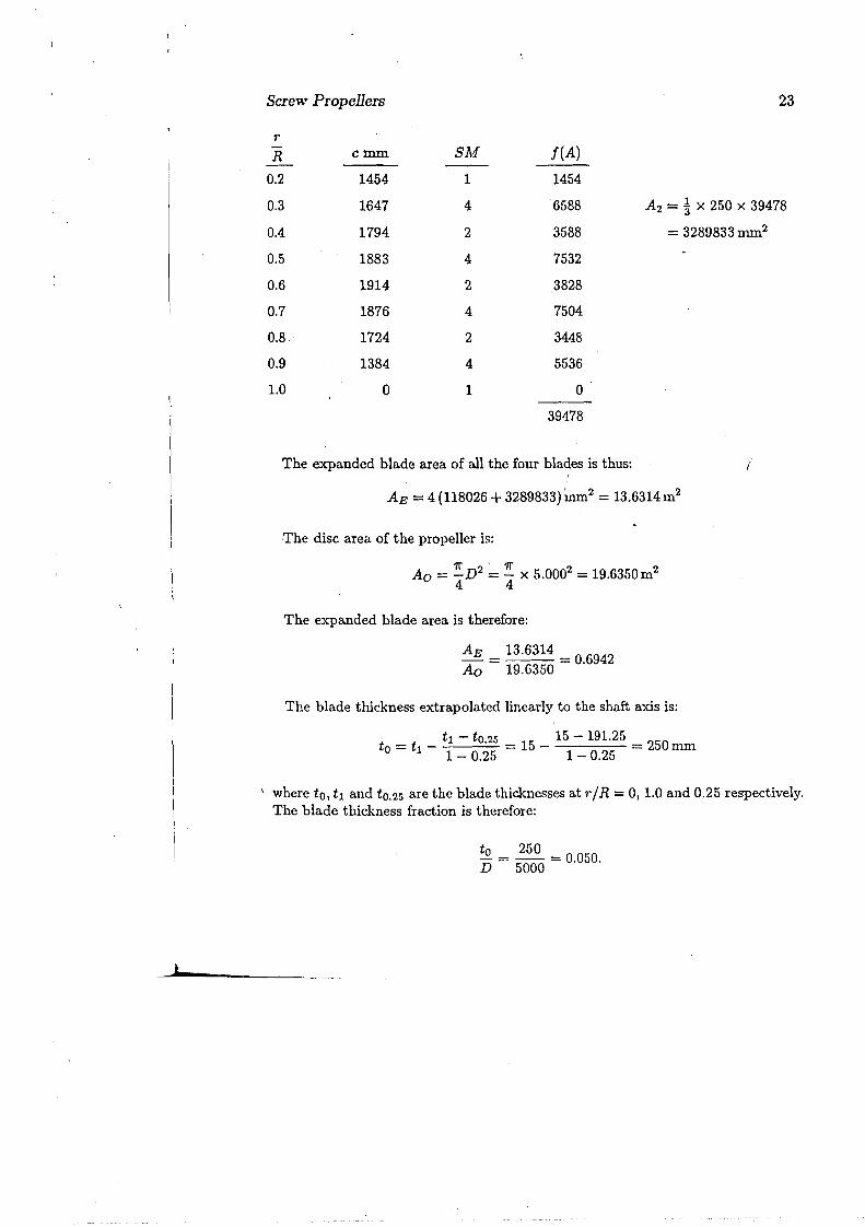
where 1/3 is the common multiplier, s is the spacing between the n equidistant values of Xi, and 8M; are the Simpson Multipliers 1,4,2,4, ... ,4,2,4, Ii n must be an odd int(~ger. Here, c is to be integrated over the radius from 0.2R to LOR, the spacing between the radii being O.lR == 250 rom. The integration is usually carried out in a table as shown in the following:

Screw Propellers 23

r cmm 8M j(A)R-

0.2 1454 1 1454

0.3 1647 4 6588 A2 = ~ x 250 x 39478

0.4 1794 2 3588 = 3289833 mm2

0.5 1883 4 7532

0.6 1914 2 3828

0.7 1876 4 7504

0.8 1724 2 3448

0.9 1384 4 5536

1.0 0 1 0

39478

The expanded blade area of all the four blades is thus: I

AE =4 (118026 +3289833)'mm2 =13.6314 m2

The disc area of the propeller is:

Ao = ~D2 =~ X 5.0002 = 19.6350m2

The expanded blade area is therefore:

A E = 13.6314 = 0.6942 Ao 19.6350

The blade thickness extrapolated linearly to the shaft axis is:

_ _ tl - to.25 _ 5 _ 15 - 191.25 _ 250 mm to - tl 1 _ 0.25 - 1 1 _ 0.25 ­

\ where to, tl and to.25 are the blade thicknesses at r / R = 0, 1.0 and 0.25 respectively. The blade thickness fraction is therefore:

to = 250 = 0.050. D 5000

I.

,,~ I 'f,a".;~

24 Ba.<;ic Ship Propulsion 'I , 1:',',

,':~Ir ~i2.7 Mass and Inertia

The mass of a propeller needs to be calculated to estimate its cost, and both the mass and the polar moment of inertia are required for determining the vibration characteristics of the propeller shafting system. The mass and polar moment of inertia of the propeller blades can be easily determined by integrating the areas of the blade sections over the radius. The mass and inertia of the boss must be added. Thus, one may write:

, i R M=Pm Z adr+Mboss (2.3)

rb

2lp = Pm Z l'R ar dr + lboss (2.4) rb

where M and lp are the mass and polar moment of inertia of the propeller, Pm is the density of the propeller material, a the area of the blade section at radius r, and Mboss and lboss the mass and polar moment of inertia of the propeller boss, the other symbols having been defined earlier..

The area of a blade section depends upon its chord c and thickness t so that for a blade section of a given type, one may write:

\ a = constant X ext (2.5)

The ~hords or blade widths at the different propeller radii are proportional to the expanded blade area ratio per blade, while the section thicknesses depend upon the blade thickness fraction. One may therefore write:

AE to 3 -"\1 - kmPm Ao D D + Mboss (2.6)

AE to 5 I p = ki Pm Ao D D + lhoss (2.7)

where km and ki are constants which depend upon the shape of the propeller blade sections. '

25 Screw Propellers

Problems

1. A propeller of 6.0 m diameter and constant pitch ratio 0.8 has a flat faced expanded section of chord length 489 nun at a radius of 1200 mm. Calculate the arc lengths at this radius of the projected and developed outlines.

2. The distances of points on the face of a propeller blade from a plane normal to the axis measured at the trailing edge and at 10degree intervals up to the leading edge at a radius of 1.75 m are found to be as follows:

TE LE Angle, deg -37.5 -30 -20 -10 o 10 20 30 32.5 Distance, mm: 750 770 828 939 1050 1161 1272 1430 1550

The propeller has a diameter of 5.0 m. The blade section has a flat face except nea~ the trailing edge (TE) and the leading edge (LE). Determine the pitch at this radius. If the propeller has a constant pitch, what is its pitch ratio?

3. The cylindrical polar coordinates (r,B,z)of a propeller, r being measured in rom from the propeller axis, (j in degrees from a reference plane through the axis and z in rom from a plane normal to the axis, are found to be (1500,

I

10, 120) at the leading edge and (1500, -15, -180) at the trailing edge at the blade section at 0.6R. The blade ~ection at this radius has a flat face. Determine the width of the expanded outline at thi~ radius and the position of the reference line, B == 0, with respect to the leading edge. What is the pitch ratio of the propeller at 0.6R? The propeller has no rake.

4. The expanded blade widths of a three-bladed propeller of diameter 4.0 m and pitch ratio 0.9 are as follows:

rjR : 0.2 0.3 0.4 0.5 0.6 0.7 0.8 0.9 1.0 cmm: 1477 1658 1808 1917 1976 1959 1834 1497 o

Find the expanded, developed and projected blade area ratios of the propeller•. Assume that the root section is at 0.2R, the blade outline is symmetrical and the blade sections are flat faced.

5. The face and back offsets of a propeller blade section with respect to a straight line joining the leading and trailing edges ("nose-tailline") are as follows:

Distance from Face offset Back offset leading edge mm nun rom

0 0 0 50 -24.2 37.8

L

Basic Ship Propulsion

Distance from Face offset Back offset leading edge mm mill rom 100. -32.4 54.8 200 -42.5 77.5 300 -48.0 91.1 400 -:..50.2 98;3 500 -49.4 99.4 600 -45.3 94.3 700 -38.3 82.8 800 -29.1 64.2 900 -19.2 37.1

1000 -5.0 5.0

Determine the thit::kness-chord ratio and the camber ratio of the section.

6. A propeller of a single screw ship has a diameter of 6.0 m and a radially varying pitch as follows:

r/R : 0.2 0.3 0.4 0.5 0.6 0.7 0.8 0.9 1.0 . P / D: 0.872 0.902 0.928 0.950 0.968 0.982 0.992 0.998 1.000

Calculate the mean pitch ratio of the propeller. What is the pitch at 0.7R?

7. , A- propeller of 5.0 m diameter and 1.1 effective pitch ratio has a speed of advance of 7.2 m per sec when running at 120rpm. Determine its slip ratio. If the propeller rpm remains unchanged, what should be the speed of advance fot., the propeller to have (a) zero slip and (b) 100 percent slip?

8. In 'a four-bladed propeller of 5.0 m diameter, each blade has an expanded area of 2.16m2 • The thickness of the blade at the tip is 15mill, while at a radius of 625 inm the thickness is 75 mm with a .linear variation from root to tip. The boss diameter is 835 mill. The propeller has a pitch of 4.5 m. Determine the pitch ratio, the blade area ratio, the blade thickness fraction and the boss diameter ratio of the propeller.

9. A crudely made propeller consists of a cylindrical boss of 200 mm diameter to which are welded three flat plates set at an angle of 45 degrees to a plane normal to the propeller axis. Each flat plate is 280 mm wide with its inner edge shaped to fit the cylindrical boss and the outer edge cut square so that the distance of its midpoint from the boss is 700 mID. Determine the diameter, the mean pitch ratio and the expanded and projected blade area ratios of this propeller.

Screw Propellers 27

10. A three-bladed propeller of diameter 4.0m has blades whose expanded blade widths and thicknesses at the different radii are as follows:

r/R 0.2 0.3 0.4 0.5 0.6 0.7 0.8 0.9 1.0 Width, mm 1000 1400 1700 1920 2000 1980 1800 1320 0 Thickness, mm ; 163.0 144.5 126.0 107.5 89.0 70.5 52.0 33.5' 15.0

The blade sections are all segmental with parabolic backs, and the"boss may be regarded as a cylinder of length 900mm and inner and outer diameters of 400 mm and 650 mm respectively. The propeller is made of Aluminium Nickel Bronze of density 7600 kg per m3 . Determine the mass and polar moment of inertia of the propeller.

CHAPTER 3

Propeller Theory

3.1 Introduction

A study of the theory of propellers is important not only for understanding the fundamentals of propeller action but also because the theory provides results that are useful in the design of propellers. Thus, for exampl~, pro­peller theory shows that even in ideal conditions there is an upper limit to the efficiency of a propeller, and that this efficiency decreases as the thrust loading on the propeller increases. The theory also shows that a propeller is most efficient if all its radial sections work at the same efficiency. Fi­nally, propeller theory can be used to determine the detailed geometry of a propeller for optimum performance in given operating conditions.

Although the screw propeller was used for ship propulsion from the be­ginnIng of the 19th Century, the first propeller theories began to be devel­oped only some fifty years later. These early theories followed two schools of thought. In the momentum theories as developed by Rankine, Green­hill and R.E. Froude for example, the origin of the propeller thrust is ex­

__ plained entirely by the change .in the momentum of the fluid due to the .' propeller. The blade element theories, associated with Weissbach, Redten­

--) bacher, W. Froude, Drzewiecki and others, rest on observed facts rather than on mathematical principles, and explain the action of the propeller ill terms of the hydrodynamic forces experienced by the radial sections (blade elements) of which the propeller blades are composed. The momentum the­ories are based on correct fundamental principles but give no indication of

28

29

I \ \

II1

Propeller Theory

the shape of the propeller. The blade element theories, on the other hand, explain the effect of propeller geometry on its performance but give the er­roneous result that the ideal efficiency of a propeller is 100 percent. The divergence between the two groups of theories is explained by the circula­tion theory (vortex theory) of propellers initially formulated by Prandtl and Betz '(1927) and then developed by a number of others 1;0 a stage where it is not only in agreement with experimental results but may also be used for the practical design of propellers.

3.2 Axial Momentum Theory

In the axial momentum theory, the propeller is regarded as an "actuator disc"which imparts a sudden increase in pressure to the fluid passing through it. The mechanism by which this pressure increase is obtained is ignored. Further, it is assumed that the resulting acceleration of the fluid and hence the thrust generated by the propeller are uniformly distributed over the disc, the flow is frictionless, there is no rotation of the fluid, and there is an un­limited inflow of fluid to the propeller. 'The acceleration of the fluid involves a contraction of the fluid column passing through the propeller disc and, since this cannot take place suddenly, the acceleration takes place over some distance forward and some distance aft of the propeller disc. The pressure in the fluid decreases gradually as it approaches the disc, it is suddenly in­creased at the disc, and it then gradually decreases as the fluid leaves the disc. Consider a propeller (actuator disc) of area Ao advancing into undis­turbed fluid with a velocity VA' A uniform velocity equal and opposite to VA is imposed on this whole system, so that there is no change in the hydrody­namic forces but one considers a stationary disc in a uniform flow of velocity VA, Let the pressures and velocities in the fluid column passing through the propeller disc be Po and VA far ahead, PI and "A +VI just ahead of the disc, P~ and VA +VI just behind the disc, and P2 and "A +V2 far behind the disc, as shov,!1 in Fig.3,1. From considerations of continuity, the velocity just ahead and just behind the disc must be equal, and since there is no rotation of the fluid, the pressure far behind the propeller must be equal to the pressure far ahead, Le. P2 = PO.

The mass of fluid flowing through the propeller disc per unit time is given by:

II

l~.

l

--

30 Basic Ship Propulsion

FLUID COLUMN

ACTUATOR DISC FAR ASTERN AREA . Ao FAR AHEAD

I -r---''-._..-.'-'_.-i=-'-'-'-'-'­PRESSURES VELOCITIES

p.'1

PRESSURE VARIATION

Figure 3.1 : Action of an Actuator Disc in the Axial Momentum Theory. .\

(3.1)

where p is the density of the fluid. This mass of fluid is accelerated from a' v.elocity VA to a velocity VA + V2 by the propeller, and since the propeller thrust T is equal to the change of axial momentum per unit time:

(3.2)

. The total power delivered to the propeller PD is equal to the increase in the kinetic energy of the fluid per unit time, i.e. :

(3.3)

.... -.-_... -.-_._-_.__ ..._....,

. Propeller Theory

This delivered power. is also equal to the work done by the thrust 011 the fluid per unit, time, .j.el

•. :. .' :.',.

It therefore follows that: (3.5)

, .

i.e. half the increase in axial velocity due to the propeller takes place ahead of it and half behind it.

The same result may be obtained in a different way. By applying the Bernoulli theorem successively to the sections far ahead and ju.st ahead of the propeller, and to the sections far behind andjust behind the prop'eiler, one obtains: .. . . ,.

. 1 21 2Po + 2" PVA = PI t 2" P(VA +Vl)

P2+ ! (VA + V2)2 = P~.+ !p(~ + Vl)2 , . "

. . .. .• ~ .~. . . ' ...!

., . ,~o that,noting that P2 =, Po:

P~ - Pl = ! P [(VA + V2)2 - VA2 j

= P (VA + ! V2) V2

. . .~

The propeller thruSt is given by:

so that by'comparing Eqns. (3.2) and (3.9), Ol~e again obtains Eq!1' (3:5).

The useful work done by the propeller per unit time is TVA. The efficiency of the propeller is therefore:

TVA T]i =-­

PD 1

l+a . (3.10)

~--~, _ _,-- --- --- _-_ - '.- -~. . .

32 Basic Ship Propulsion

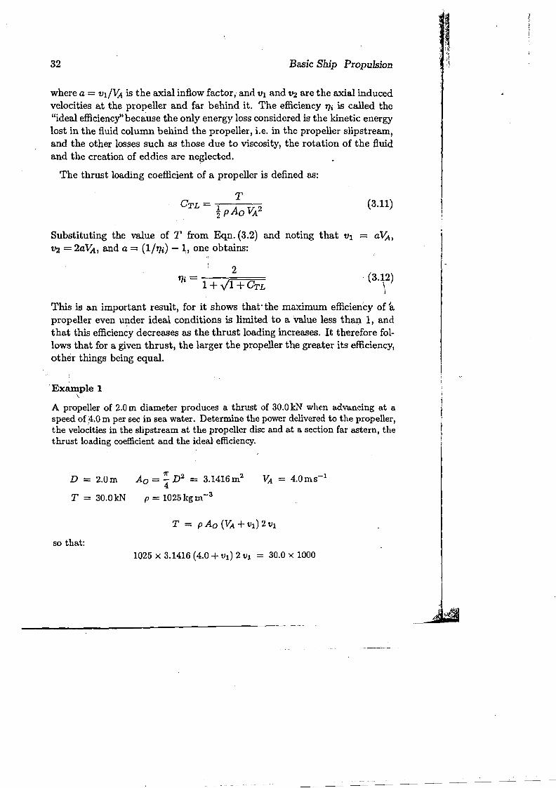
where a= vI/VA is the axial inflow factor,· and VI and V2 are the axial induced velocities at the propeller and far behind it. The efficiency 'f}i is called the "ideal efficiency" because the only energy loss considered is the kinetic energy lost in the fluid column behind the propeller, i.e. in the propeller slipstream, and the other losses such as those due to viscosity, the rotation of the fluid and the creation of eddies are neglected.

The thrust loading coefficient of a propeller is defined as:

T (3.11)CTL = 1 A v: 2

"2 P 0 A

Substituting the value of T from Eqn. (3.2) and noting that VI = a't-A, V2 =2aVA, and a = (1/'f}i) - 1, one obtains:

2 (3.12)

'f}i = 1+ \1'1 +CTL \ i

This is an important result, for it shows that'themaximum efficiency of-a propeller even ullder ideal.conditions is limited to a Value less than 1, and that this efficiency decreases as the thrust loading increases. It therefore fol­lows that for a given thrust, the larger the propeller the greater its efficiency, other things being equal.

Example 1 \

A propeller of 2.0 m diameter produces a thrust of 30.0 leN when advancing at a speed of ;4.0 m per sec in sea water. Determine the power delivered to the propeller, the velocities in the slipstream at the propeller disc and at a section far astern, the thrust loading coefficient and the ideal efficiency.

D == 2.0m Ao =~ D2 = 3.1416m2

T == 30.0leN p = 1025kgm-3

so that: 1025 x 3.1416 (4.0 + vd 2 Vl = 30.0 x 1000

33 Propeller Theory

which gives:

VI = 0.9425ms-1

a = 0.2356

V2 = 1.8850ms-1

1 -- 0.80937Ji = = 1+a

TVA 30.0 X 4.0PD = = = 148.27kW

0.80937Ji

T 30.0 X 1000CTL = = = 1.1645 ~pAOVA2 ~ X 1025 X 3.1416 X 4.02

If GTL r~duces to zero, i.e. T = 0, the ideal efficiency TJi becomes equal to 1. If, on the other hand, "A tends to zero, TJi also tends to zero, although the propeller still produces thrust. The relation between thrust and delivered power at zero speed' of advance is of interest since this condition represents

1, the practical situations of a tug applying astatic pull at a bollard or of a ship at a dock trial. For an actuator disc propeller, .the delivered power is given by:

(3.13)

As 1(4. tends to zero, 1 + VI + GTL tends to VCTL' so that in the limit:

= [ T3 ]~ 2p A o

//

that is,

(3.14)

.L

34 Basic Ship Propulsion

This relation between thrust and delivered power at zero velocity of ad­vance for a propeller in ideal conditions thus has a value of y'2. In actual practice, the value 'of this relation is considerably less.

Example 2

A propeller of 3.0 m diameter absorbs 700 kW in the static condition in sea water. What is its thrust?

D = 3.0m Ao PD = 700kW

p = 1025kgm-3

T 3 = 2p.4.oP'i> = 2 X 1025 x 7.0686 X (700 X 1000)2 kgm-3 m2(Nms-1)2

= 7100.39 X 1012 N3

T = 192.20kN

3.3 Momentum Theory Including Rotation

In \this theqry, also sometimes called the impulse theory, the propeller is regar:ded as imparting both a.."Cial and angular acceleration to the fluid flowing throlfgh the propeller disc. Consider a propeller of disc area Ao advancing into un,disturbed water with an axial velocity l-A. while revolving with an angular velocity w. Impose a uniform velocity equal and opposite to l-A on the whole system so that the propeller is revolving with an angular velocity w at a fixed position. Let the axial and angular velocities of the fluid then be VA + Vl and Wl at the propeller disc and VA +V2 and W2 far downstream, as shown in Fig. 3.2. The mass of fluid flowing per unit time through an annular element between the radii rand r + dr is' given by:

dm = pdAo (VA +vd (3.15)

where dAo is the area of the annular element.

35 Propeller Theory

ACTUATOR DISC AREA Ao

FAR ASTERN ANGULAR VELOCITY w FAR AHEAD

FLUID VELOCITIES

VA,+v2 AXIAL VA+v,

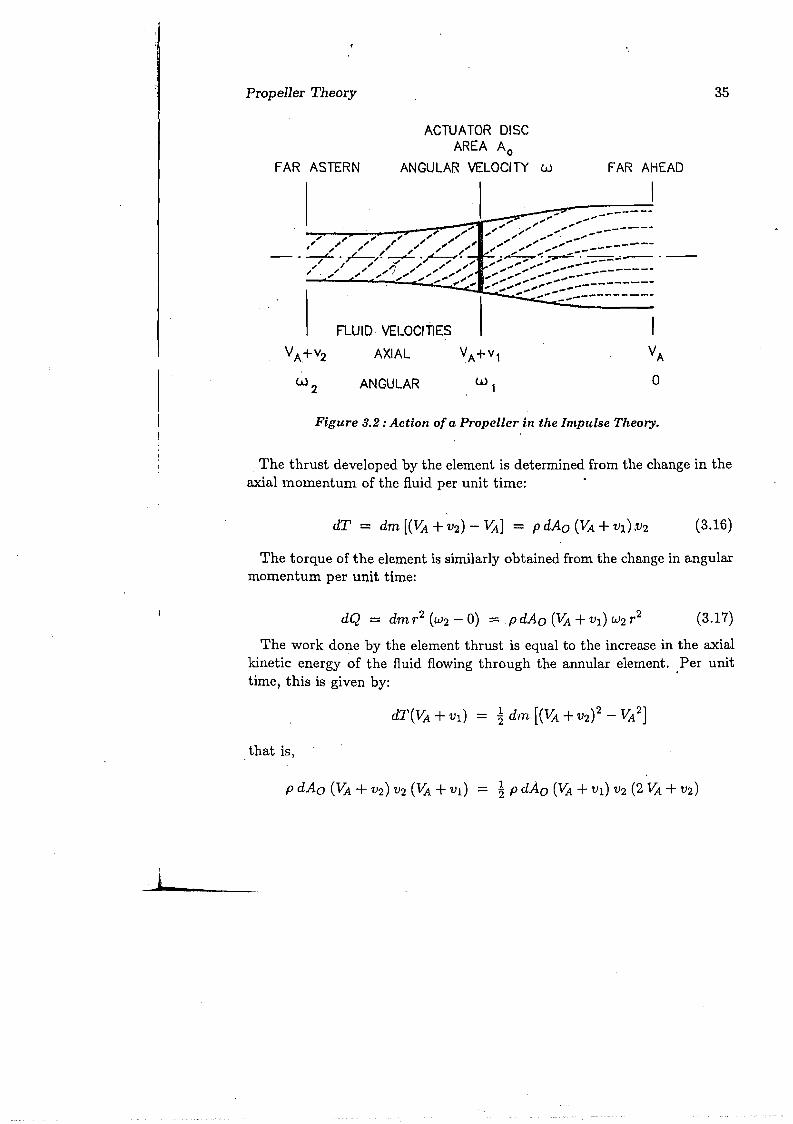
W 2 ANGULAR w, Figure 3.2: Action of a Propeller in the Impulse Theory.

. The thrust developed by the element is determined from the change in the axial momentum of the fluid per unit time:

(3.16)

The torque of the element is similarly obtained from the change in angular momentum per unit time:

(3.17)

The work done by the element thrust is equal to the increase in the axial kinetic energy of the fluid flowing through the annular element..Per unit time, this is given by:

that is,

~L _

36 Basic Ship Propulsion

so that:

(3.18)

This is the same result as obtained in the axial momentum theory, Eqn. (3.5). The work done per 1,1nit time by the element torque is simi~

larlyequal to the increase in the rotational kinetic energy of the fluid per unit time, i.e. :

dQWI - ~,dmr2 [w~ - 0]

- ~ p dAo("A + VI) W2 r 2 W2

- ~ dQ W2

so that,

WI - ~ W2 ;'(3.19)

Thus, half the angular velocity of the fluid is acquired before it reaches the propeller and half after the fluid leaves the propeller.

The total power expended by the element must be equal to the increase in the, total kinetic energy (axial and rotational) per unit time, or the work done by the element thrust and torque on the fluid passing through the element ,per unit time:

that is,

and the efficiency of the element is then:

(W - WI)"A 1-~ 1- a' = W = (3.20)("A + VI) W l+~ l+a

Propeller Theory 37

where a' = wl/w and a = vl/VA are the rotational and axial inflow factors, VI and V2 are the axial, induced velocities at the propeller and far down­stream, Wl and W2 being the corresponding angular induced velocities. It may be seen by comparing this expression for efficiency, Eqn. (3.20), with theexpression obtained in the axial momentum theory, Eqn. (3.10), that the effect of slipstream rotation is to reduce the efficiency by the factor (1- a') ..

By making the substitutions:

dAo - 21r r dr, Vl - a"A,

Wl = a' w W2 - 2a' w

in Eqns. (3.16) and (3.17), one obtains:

/' dT - 41rprdr"A2 a(1+a) (3.21)" . /dQ - 41rpr3 dr"ACLI'a'(1+a) (3.22)

The efficiency of the annular element is!'then given by:

dTVA 41r Pr dr "A2 a(l+ a)"A . a VA 2

7] = (3.23)dQw - 41rpr3 drVAwa'(1+a)w = a' w2 r2

Comparing this with Eqn. (3.20), one then obtains:

or, 2a' (1 - a') w2 r = a (1 + a) VA2 (3.24)

This gives the relation between the axial and rotational induced velocities in a propeller when friction is neglected.

Example 3

A propeller of diameter 4.0 m has an rpm of 180 when advancing into sea water at a speed of 6.0 m per sec. The element of the propeller at 0.7R produces a thrust of 200 kN per m. Determine the torque, the axial and rotational inflow factors, and the efficiency of the element.

38 Basic Ship Propulsion

D == 4.0m n == 180rpm = 3.05-1 VA = 6.0ms-1

r == 0.7R'== 0.7x2.0 = 104m dT dr

== 200kNm-1

w = 211" n == 611" radians per sec

so that,

which gives,

that is,

or,

411" x 1025 x 1.4 X 6.02 a(l + a) = 200 x 1000

a == 0.2470

a' (1 -a') w 2 r 2 == a (1 + a) VA 2

a'(l - a')(611")2 x 1.42 == 0.2470(1 +0.2470) x 6.02

a' == 0.01619

dQ == 471" Pr 3 VA w a' (1 + a)

dr

_ 471" x 1025 X 1.43 x 6.0 X 671" x 0.01619 x 1.2470

1== 80.696 kN m m­

1- a' 1 - 0.01619 == 0.78891] = == l+a 1 +0.2470

dT VA 200 x 6.0 dr == 0.7889== == 80.696 X 671"~w

j

I

l·~l, ' .~ I

39 Propeller Theory

3.4 Blade Element Theory

The blade element theory, in contrast to the momentum theory, is concerned with how the propeller generates its thrust and how this thrust depends upon the shape of the propeller blades. A propeller blade is regarded as being com­posed of a series of blade elements, each of which produces a hydrodynamic

/ force due to its motion through the fluid. The axial,component of this hydro­dynamic force is the element thrust while the moment ~bout the propeller axis of the tangential component is the element torque. The integration of the element thrust and torque over the radius for all the blades gives the total thrust and torque of the propeller.

L

o

1s

~J ~c---J

Figure 3.3: Lift and Drag of a Wing.

Consider a wing of chord (width) c and span (length) s at an an­gle of attack Q to an incident flow of velocity V in a fluid of den­sity p, as shown in Fig. 3.3. The wing develops a hydrodynamic force whose components normal and parallel to, V are the lift L and the drag D. One defines non-dimensional lift and drag coefficients as follows:

J___

-

40 Basic Ship Propulsion

L ~pAV2

(3.25)D

CD = ~pAV2

, . where A = s c is the area of the wing plan form. These coefficients depend upon the shape of the wing section, the aspect ratio sic and the angle of attack, and are often determined experimentally in a wind tunnel. These experimental yalues may then be used in the blade element theory, which may thus be said to rest on: observed fact.

(0) WITHOUT INDUCED VELOCITIES

dD ~__-2nnr ---­

\.

(b) WITH INDUCED VELOCITIES

Figure 3.4 : Blade Element Velocities and Forces.

Now consider a propeller with Z blades, diameter D and pitch ratio PID advancing into undisturbed water with a velocity VA while turning at a rev­olution rate n, The blade element between the radii rand r + dr when expanded will have an incident flow whose axial and tangential vel<:Jcity components are VA and 211" n r respectively, giving a resultant velocity VR

41

"-Jr-- ~

Propeller Tbeory f<J.-!l!tc

~ /~ /. ­

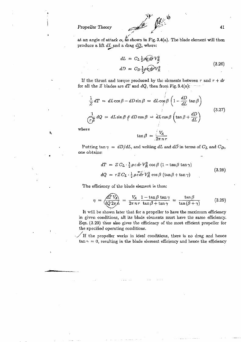
at an angle of attack a, ~ shown in Fig. 3.4(a). The blade element will then produce a lift d!,:-and a drag eyh where:

(3.26)

If the thrust and torque produced by the elements between rand r + dr for all the Z blades are dT and dQ, then from Fig. 3.4(a);···-·'

1 j ( dD )Z dT = dLcos f3 - dD sinf3 = dLcisf3 1- dL tanf3

(3.27)

@dQ = dL sin{3 f dD cos {3 = ;ll/cos {3 (tan (3 + ~~) where

I VA tan{3 ='-­

,21rnr

Putting tan')' = dDjdL, and writing dL and dD in terms of CL and CD, one obtains:

•

dT - Z GL' ~ pcdr VJ cosf3 (1- tanf3 tan')') (3.28)

dQ - r Z CL . ~ p;d~ VA cos f3 (tan f3+ tan')')

The efficiency of the blade element is then:

@ "" 1 - tan (3 tan ~ tan{3 7J = dQ21r = 21rnr tan{3 + tan')' :::: tan(f3 + ')') (3.29)

It "'ill be sho~n later that for a propeller to have the maximum efficiency in given conditions, all its blade elements must have the same efficiency. Eqn. (3.29) thus also gives the efficiency of the most efficient propeller for the specified operating conditions.

../If the propeller works in ideal conditions, there is no drag and hence tan..... = 0, resulting in the blade element efficiency and hence the efficiency

42 Basic Ship Propulsion

of the most efficient propeller being 1] = 1. This is at variance with the

j esuIts of the momentum theory which indicates that if a propeller produces a thrust greater than zero, its efficiency even in ideal conditions must be less than 1.

J The primary reason for this discrepancy lies in the neglect of the induced velocities, i.e. the inflow factors a, a'. If the induced velocities are (;ak~ ac~, as shown in Fig. 3.4(b), one obtains:

dT = ZCL·~pcdrV~cos!h (l-tan,Bltan,) (3.30)

dQ = r Z CL . ~ Pc dr V~ cos (3I (tan,B[ + tan,)

and:

dTVA· VA 1'- tan,BI tan, tan,B 1] = - =

dQ2ran 271" n r tan,B[ + tan,

tan,B tan ,B[ 1 - a' tan,B[=--. = .(3.31)

tan,B[ tan (,B[ +,) 1 + a tan (,BI +,)

since,

VA "A (1 + a) l+atan,B = and tan,B[ = = tan,B 1 - a'271" n r 271"nr(1-a')

In Eql1. (3.31), the expression for efficiency consists of three factors: (i) 1/(1 t a), which is associated with the axial induced velocity, Eqn. (3.10), (ii) (1 - a'), which reflects the loss due to the rotation of the slipstream, and (iii) tan,BrI tan(,B[ + ,), which indicates the effect of blade element drag. If there is no drag and tan, = 0, the expression for efficiency, Eqn. (3.31), becomes identical to the expression obtained from the impulse theory, Eqn. (3.20).

In order to make practical use of the blade element theory, it is necessary to know CL, CD, a and a' for blade elements at different radii so that dT/dr and dQ/dr can be determined and integrated with respect to the radius r. CL and CD may be obtained from experimental data, and a and a' with the help of the momentum theory. Unfortunately, this procedure does not y~eld

realistic results because it neglects a number of factors.

Propeller Theory 43

Example 4

A four bladed propeller of 3.0 m diameter and 1.0 constant pitch ratio has a speed of advance of 4.0 m per sec when running at 120 rpm. The blade section at 0.7R has a chord of 0.5 m, a no-lift angle of 2 degrees, a lift-drag ratio of 30 and a lift coefficient that increases at the rate of 6.0 per radian for small angles of attack. Determine the thrust, torque and efficiency of the blade element at 0.7R (a) neglecting the induced velocities and (b) given that the axial and rotational inflow factors are 0.2000 and 0.0225 respectively.

PZ=4 D = 3.0m D = 1.0

n = 120rpm = 2.0 s-l

rx= Ii = 0.7 c = 0.5m = 30

= 6.0 per radian p ~' 1025kgm-3

(a) Neglecting induced velocities:

tanlp = P/D = 1.0 = 0.4547 If> = 24.4526°71" X 71" x 0.7

VA 4.0tan!, = = = 0.3032 f3 = 16.8648°

271"nr 271" X 2.0 x (0.7 x 1.5)

tan...,' = CD = ~ = 0.03333 'Y = 1.9091° CL 30

o· = If> - {3 = 7.5878°

8CL 6.0 2 + 7.5878CL = 80: (0:0+0:) = = 1.0040

180/71"

~r2 = ~2 + (271"nr)2 4.02 + (271" X 2.0 X 1.05)2R =

= 190.0998 m2 S-2

dT = Z CL 4pc vJ cos {3 (1 - tan{3 tan 1')

dr

.J.__

44 Basic Ship Propulsion

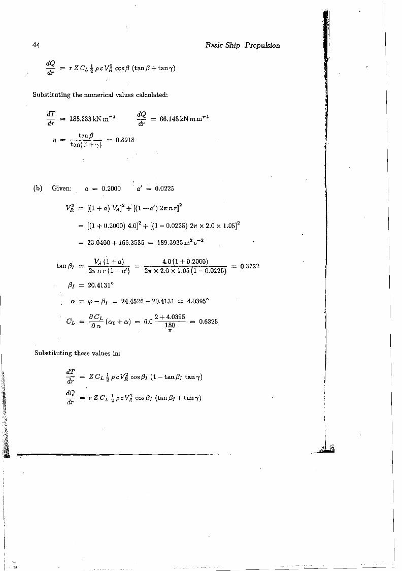
dQ dr = r Z CL ~ Pc V~ cos f3 (tan f3 + tan')')

Substituting the numerical values calculated:

dT = 185.333 k.l~ m-1 dQ = 66.148kNmm:"1 dr dr

tanf3 1] = = 0.8918

tan(3+:)

(b) Given: a = 0.2000 . a' ~ 0.0225

v~ ::: [(1 + a) \'A]2 + [(1-a') 271"nr]2

::: [(1 + 0.2000) 4.0]2 + [(1 - 0.0225) 271" x 2.0 X 1.05]2

= 23.0400 + 166.3535 ::: 189.3935 m2s-2

~... (1 + a) 4.0 (1 + 0.2000) = 0.3722tanf3I = = 271"nr(1-a') 271" x 2.0 x 1.05 (1 - 0.0225)

PI = 20.4131 0

a: = !p - f3I = 24.4526 - 20.4131 = 4.03950

2+ 4.0395 6.0 180 = 0.6325

7r

Substituting these values in:

dT dr = Z CL ~ pcV~ cosf3r (1- tanf3r tan')')

dQ 1 2dr = 7'ZCL 2 PcVRcosf3I (tanth+tan')')

, -f$:

45 Propeller Theory

one obtains:

dT = 113.640kNm-1

dr

dQ = 48.991 kNmm-1

dr

1- a' tan(3r 1- 0.0225 0.3722 1] = x-- = 0.7383= 1 +a tan((3r + "Y) 1 +0.2000 0.4104

3.5 Circulation Theory

vr=k

The circulation theory or vortex theory provides a more satisfactory explanation of the hydrodynamics of propeller action than the momentum and blade element theories. The lift produced by each propeller blade is

~xplained in terms of the circulation arou;nd it in a manner analogous to the lift produced by an aircraft wing, as described in the following. .

: I ~ ~ ::.V+V ..

: & :-v~ .~ =::::..v-v~

I i

(0) VORTEX (b) UNIFORM (c) VORTEX IN FLOW FLOW UNIFORM FLOW

Figure 3.5: Flow olan Ideal Fluid around a Circular Cylinder.

Consider a flow in which the fluid particles move in circular paths such that the velocity is inversely proportional to the radius of the circle, Fig.3.5(a). Such a flow is called a vortex flow, and the axis about which the fluid particles move in a three dimensional flow is called a vortex line. In an ideal fluid, a vortex line cannot end abruptly inside the fluid but must either form a closed curve or end on the boundary of the fluid (Helmholz theorem). A circular cylinder placed in a uniform flow of an ideal fluid, Fig. 3.5(b), will experience

1___

46 Basic Ship Propulsion

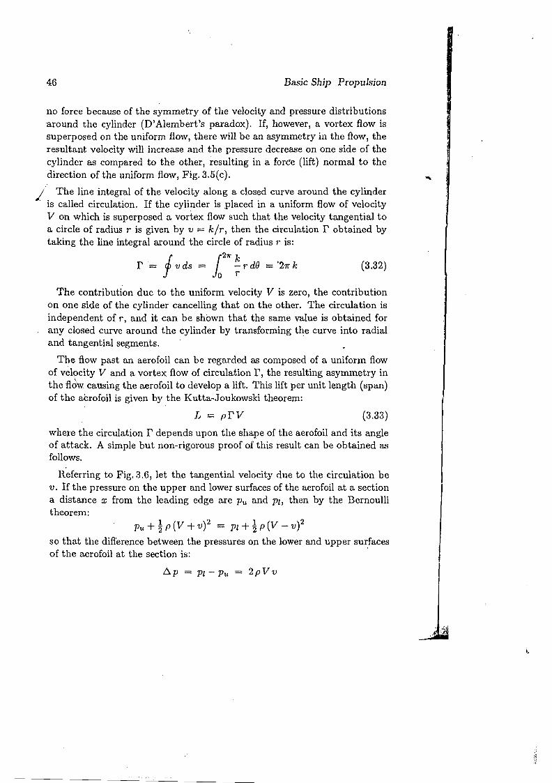
no force because of the symmetry of the velocity and pressure distributions around the cylinder (D'Alembert's paradox). If, however, a vortex flow is superposed on the uniform flow, there will be an asymmetry in the flow, the resultant velocity will increase and the pressure decrease on one side of the cylinder as compared to the other, resulting in a force (lift) normal to the direction of the uniform flow, Fig.3.5(c). '"

I' The line integral of the velocity along a closed curve around the cylinder . is called circulation. If the cylinder is placed in a uniform flow of velocity

V on which is superposed a vortex flow such that the velocity tangential to a circle of radius r is given by v = k/r, then the circulation r obtained by taking the line integral around the circle of radius r is:

21r

r= f v ds = 1 ~ r dB = '27r k (3.32)

The contribution due to the uniform velocity V is zero, the contribution on one side of the cylinder cancelling that on the other. The circulation is independent of r, and it can be shown that the same value is obtained for any closed curve around the cylinder by transforming the curve into radial and tangential segments.

The flow past an aerofoil can be regarded as composed of a uniform flow of velocity V and a vortex flow of circulation r, the resulting asymmetry in the floW: causing the aerofoil to develop a lift. This lift per unit length (span) of the aerofoil is given by the Kutta-Joukowski theorem:

L = pry (3.33)

where the circulation r depends upon the shape of the aerofoil and its angle of attack. A simple but non-rigorous proof of this result can be obtained as follows.

Referring to Fig. 3.6, let th.e tangential velocity due to the circulation be v. If the pressure on the upper and lower surfaces of the aerofoil at a section a distance x from the leading edge are Pu and PI, then by the Bernoulli theorem:

Pu + ! p (V + v)2 = PI + ! p (V - v)2

so that the difference between the pressures on the lower and upper surfaces of the aerofoil at the section is: '

6. P = PI - Pu = 2 p V v

'---_dX_~~~x t

I Propeller Tbeory 47

yv

x __-\--- ...:;. -'1.-.10 ...... ......--- V

v

Figure 3.6: Circulation around an Aerofoil.

If the x-coordinate of the trailing edge lis Xl, the lift produced by the aerofoil per unit length (span) is:

L = l·['t>.PdX = pV['2VdX = pLC~dX+ J.:-VdX] V - pry

as given in Eqn. (3.33).

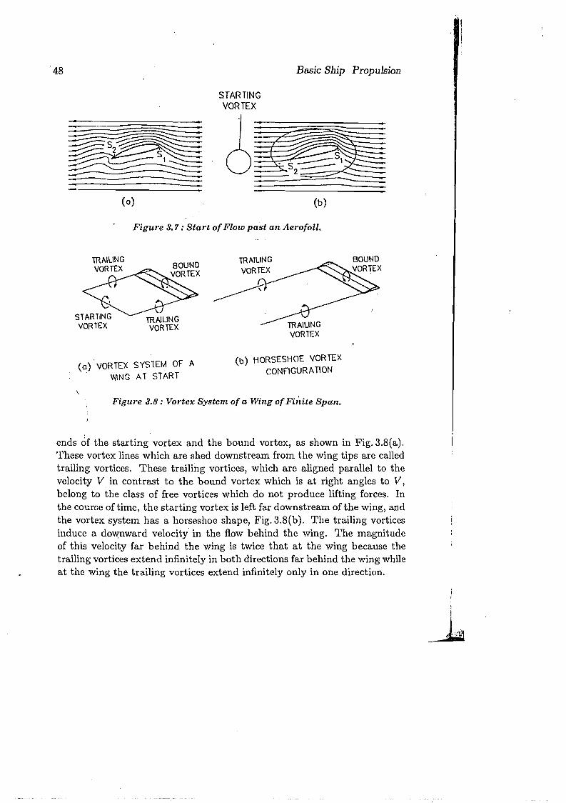
If a wing of infinite aspect ratio with an aerofoil cross-section is given a velocity V, the flow around it is initially as shown in Fig.3.7(a), with a stagnation point 51 near the leading edge and a stagnation point 52 upstream of the trailing edge on the upper surface with flow taking place around the trailing edge towards 52 in an adverse pressure gradient. Such a flow is unstable and as a result a vortex is shed from the trailing edge causing the stagnation point 52 to move to the trailing edge and a circulation to develop around the wing, Fig. 3.7(b). The vortex, which is shed from the aerofoil at the start of the flow is called the starting vortex while the vortex associated with the circulation around the wing is called the bound vortex.

In a wing of finite span, the starting vortex land the bound vortex cannot end abruptly in the fluid and there must exist vortex lines which connect the

,

lc_­

48 Basic Ship Propulsion

STARTING VORTEX

:;;. ----­­

(0) (b)

Figure 3.7: Start ofFlow past an Aerofoil.

mAILING VORTEX

(b) HORSESHOE VORTEX(0) .VORTEX SYSTEM OF A

CONFIGURATlON . W1NG AT START

\

Figure 3.8: Vortex System of a Wing ofFiliite Span.

ends of the starting vortex and the bound vortex, as shown in Fig.3.8(a). These vortex lines which are shed downstream from the wing tips are called trailing vortices. These trailing vortices, which are aligned parallel to the velocity V in contrast to the bound vortex which is at right angles to V, belong to the class of free vortices which do not produce lifting forces. In the course of time, the starting vortex is left far downstream of the wing, and the vortex system has a horseshoe shape, Fig.3.8(b). The trailing vortices induce a dow:nward velocity in the flow behind the wing. The magnitude of this velocity far behind the wing is twice that at the wing because the trailing vortices extend infinitely in both directions far behind the wing while at the wing the trailing vortices extend infinitely only in one direction.

49 Propeller Theory

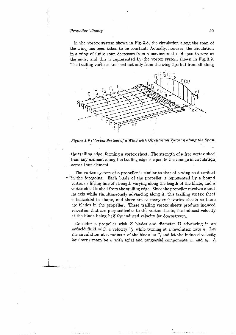
In the vortex system shown in Fig. 3.8, the circulation along the span of the wing has been taken to be constant. Actually, however, the circulation in a wing of finite span decreases from a maximum at mid-span to zero at the ends, and this is represented by the vortex system shown in Fig. 3.9. The trailing vortices are shed not only from the wing tips but from all along

Figure 3.9: Vortex System of a Wing with Circulation Varying along the Span.

the trailing eage, forming a vortex sheet. The strength of a free vortex shed from any element along the trailing edge is equal to the change in ~irculation_

\ across that element.

The vortex system of a propeller is similar to that of a wing as described '''----In the foregoing. Each blade of the propeller is represented by a bound

vortex or lifting line of strength varying along the length of the blade, and a vortex sheet is shed from the trailing edge. Since the propeller revolves about its axis while simultaneously advancing along it, this trailing vortex sheet is helicoidal in shape, and there are as many such vortex sheets as there are blades in the propeller. These trailing vortex sheets produce induced velocities that are perpendicular to the vortex sheets, the induced velocity at the blade being half the induced velocity far downstream.

Consider a propeller with Z blades and diameter D advancing in an inviscid fluid with a velocity VA while turning at a revolution rate n. Let the circulation at a radius r of the blade be f, and let the induced velocity far downstream be u with axial and tangential components U a and Ut. A

~---

50 Basic Ship Propulsion

TRAILING TRAILING BOUND VORTEX VORTEX .1/ VORTEX AT RADIUS r SHEET

\ r Q

U '~-==/:.~=iW-\:t=\==~~==l l' ----~--.r---~A 1n .

FAR FAR ASTERN AHEAD

Z = 4 I

V ! .cbr I I

IcPr

U t i

9r .

0 2JTr

I cbr

v I \

Figure 3.10: Vortex System of a Propeller.

relationship between the circulation r and the induced velocity Ut is found by taking the line integral of the velocity along the closed curve defined by the ends of a cylinder of radius r. extending from far ahead of the propeller to far behind it, the end circles being connected by two parallel straight lines very close to each other, as shown in Fig. 3.10. The velocity along the circle far ahead is zero and along the circle far astern is Ut. The line integrals along the two parallel straight lines cancel each other, so that the circulation is obtained as:

zr 27r rUt (3.34)

. :

__

51

VA

~-~----+-J1

Propeller Theory

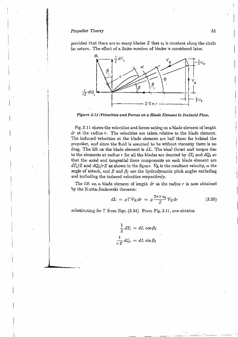
provided that there are so many blades Z that Ut is constant along the circle far astern. The effect of a finite number of blades is considered later.

'_1 dQ l4--~I::.--_--->~rZ i ~L

t u~__"'--__ 2 nn r ~ .~~ . t

Figure 3.11 :Velocities and Forces on a Blade.Element in Inviscid Flow.

Fig. 3.11 shows the velocities and forces acting on a blade element of lengthI

dr at the radius r. The velocities are tak~n relative to the blade element. The induced velocities at the blade element are half those far behind the propeller, and since the fluid is assumed to be without viscosity there is no drag. The lift on the blade element is dL. The ideal thrust and torque due to the elements at radius r for all the blades are denoted by dT;. and dQi so that the axial and tangential force components on each blade element are dT;,/Z and dQi/rZ as shown in the figure. VR is the resultant velocity, Q the angle of attack, and {3 and {3I are the hydrodynamic pitch angles excluding and including the induced velocities respectively..

The lift on a blade element of length dr at the radius r is now obtained by the Kutta-Joukowski theorem:

27frUt V' d p-- R r (3.35)

Z

substituting for r from Eqn. (3.34). From Fig. 3.11, one obtains:

1 z dTi = dL cos {3I

1 -z dQi = dL sin {3I7'

52 Basic Ship Propulsion

so that, using Eqn. (3.35):

dTi - 27l" pUt VR cos (3r r dr (3.36)

dQi - 21rpUt VR filin(3rr 2 dr

and:

I dTiVA VA cos (3r tan (3---- (3.37)77i - = ­dQi 21r nr 21r n r sin (3] tan (3]

where 77~ is the ideal efficiency of the blade section at radius r.

One may now derive the condition for a propeller of maximum efficiency, or the "minimum energy loss condition"derived by Betz (1927). Suppose that there are two radii rl and r2 where the blade element efficiencies are 77h and 77b, with 77h being greater than 77h. It is now possible to modify the design of the propeller (by changing, the radial distribution of pit~h, for example) in such a way that the torque is increased by a small amount at the radius rl and decreased by an equal amount at the radius r2' However, because 77h is greater than 77i2' the increase in thrust at rl will be greater in magnitude than the decrease in thrust at r2. There will thus be a net increase in the total thrust T i without any increase in the total torque Qi of th~ propeller, and hence an increase in its efficiency. This process of increasing the efficiency of the propeller can be continued so long as there exist two radii in the propeller where the blade element efficiencies are not equal. If the efficiencies of the blade elements at all the radii from root to tip are equal, then the efficiency of the propeller cannot be increased further, and one has a propeller of the highest efficiency or minimum energy loss. The condition for minimum energy loss is therefore that 77;1 be independent of r, i.e. for all radii:

tan (3 1 V;ttan(31 = -- = --- (3.38)

77i 77i 21r n r

where l]i = 77; aild is the ideal efficiency of the propeller. Eqn. (3.38) implies that the vortex sheets shed by the propeller blades have the form ofhelicoidal surfaces of constant pitch VA !(77i n).

Jt I

53

! !

I Propeller Theory

From the blade section velocity diagram in Fig. 3.11, it can be shown that:

VR cos (f3J - (3)=

VA sin{3

1 tan{3J - tan{32 Ua =

VA tan{3 (1 + tan2 (31)

! Ut tan{3J (tan{31 - tan(3) =

VA tanf3 (1 + tan2 (31)

(3.39)

The ideal thrust loading coefficient is defined as:

o . _ 11 TLt - 1 A v: 2

2P 0 A

where Ao = 1r D2 /4 is the disc area of the propeller. The ideal thrust loading coefficient for a blade element at radius r is then:

= 27r pUt Vn cosf31 rdr

EpD2 VA 2

16 Ut VR cos f31 r dr D2 "A2

(3.40)

\ Using Eqns. (3.38), (3.39) and (3.40), one can write:

dCTLi ~ = I(A,TJi, r) (3.41)

so that:

CTLi = I-I (A, 1]i, r)dr = F(A,1]i)

where A = VA /1rnD = r tanf3/R. The function F(A,fJi) was calculated by Kramer (1939) for different values of Z, the number of blades. His results are usually given in the form of a diagram. The Kramer diagram, which often forms the starting point for designing a propeller using the circulation theory, is given later.

In determining the circulation r around a propeller blade at radius r, Eqn. (3.34), it has been assumed that the tangential induced velocity Ut is

J. _

l

.\\

r ~ r~~"b

!*'jUI"IlI,lt

54 Basic Sbip Propulsion

constant along the circular path in the slipstream far behind the propeller. This implies that the propeller has an infinite number of blades. The effect of a finite number of blades was calculated by Goldstein (1929) for a propeller having an optimum distribution of circulation. The effect of a finite number of blades is taken into account by incorporating a correction factor, the Goldstein factor t\, , in Eqn. (3.34) and the subsequent equations based on it. Goldstein factors have been calculated and are given in the form of diagrams with t\, as a function of tan Ih and x = r / R for different values of Z. The use of Goldstein factors to account for the finite number of blades in a propeller is valid only for a lightly loaded propeller operating in a uniform velocity field and having an optimum distribution of circulation. When these conditions are not fulfilied, it is more correct to use the induction factors calculated by Lerbs (1952). However, the Goldstein factors are much simpler to use than the Lerbs induction factors. Many propeller design methods based on the circulation theory therefore use the Goldstein factors.

In order to use the circulation theory for propeller design, it is necessary to be able to calculate the lift coefficient required at each blade section of the propeller. By definition, the lift coefficient for the blade section 'at radius r is given by:

(3.42)

Substituting for dL from Eqn. (3.34) after incorporating the Goldstein fac­tor, one obtains:

so that:

CL ~ = ~ x t\, sinlh tan(/h - f3) (3.43)

where c is the chord length of the blade section at radius r I x = r / R, and use has been made of the Eqns. (3.39). Eqn. (3.43) is used to determine the detailed geometry of the blade sections when designing a propeller. The use of the circulation theory in propeller design is considered in Chapter 9.

55 Propeller Theory .

Example 5

A propeller of 5.0 m diameter has an rpm of 120 and a speed of advance of 6.0 m per sec when operating with minimum energy loss at an ideal efficiency of 0.750. The root section is at 0.2 R. Determine the thrust and torque of the propeller in an inviscid fluid neglecting the effect of a finite number of blades.

D = 5.0m n = 120rpm = 2.0s-1

r p = 1025kgm-3 Root section x == - = 0.2

R

tan{J7]; = 7]i = 0.750 =

tan{J[

6.0 0.190986tan{J = = ------=

7r X 2.0 x x x 5.0 x

tan{J tan{Jtan{J[ = 7 = 0.750

~Ut = tan{J[ (tan{J[ - tan{J) V -'\1: cos({J[ - (J) R - A sin{JVA tan {J (1 + tan2 (3[)

dT, dr

The subsequent calculation is carried out in a tabular form, using Simpson's rule for the integration.

x r tan{J tan{J[ ~utlVA Ut {3[o {J0

m ms- 1

0.2 0.500 0.9549 1.2732 0.1619 1.9430 51.8540 43.6793 0.3 0.750 0.6366 0.8488 0.1645 1.9734 40.3255 32.4816 0.4 1.000 0.4775 0.6366 0.1510 1.8121 32.4816 25.5228 0.5 1.250 0.3820 0.5093 0.1348 1.6176 k6.9896 20.9055 0.6 1.500 0.3183 0.4244 0.1199 1.4385 22.9970 17.6568 0.7 1.750 0.2728 0.3638 0.1071 1.285~ 19.9905 15.2610 0.8 2.000 0.2387 0.3183 0.0963' 1.1561 17.6568 13.4270

J..__

56

~r

it Basic Sbip Propulsion '1,

x r tanf3 tanf3I ~utlVA Ut f3ro f3 0 .' m ms-1

0·9 2.250 0.::n22 0.2829 0.0873 1.0479 15.7984 11.9808 1.0 2.500 0.1910 0.2546 0.0797 0.9566 14.2866 10.8125

x VR dTi/dr d,Qi/dr 8M f(Ti ) f(Qi) ms-1 kNm- 1 kNmm- 1 kNm-1 kNmm-1

0.2 8.5996 33.2342 21.1576 1 33.2342 21.1576 0.3 11.0680 80.4315 51.2044 4 321.7260 204.8176 0.4 13.8228 136.0798 86.6308 2 272.1596 173.2616 0.5 16.7200 194.0184 123.5160 4 776.0736 494.0640 0.6 19.6956 251.9514 160.3973 2 503.9028 320.7946 0.7 22.7172 309.1963 196.8405 4 1236.7852 787.3620 0.8 25.7687 365.6541 232.7829 2 731.3082 465.5658 0.9 28.8399 421.3677 268.2506 4 1685.4708 1073.0024 1.0 31.9248 476.4799 303.3362 1 476.4799 303.3362

6037.1403 3843.3618

Ii = '31 x (0.1 x 2.5) x 6037.1403 = 503.095 kN

Qi = '31 x (0.1 x 2.5) x 3843.3618 = 320.280kNm

503.095 x 6.0 \, = = 0.7500 ::: 1J~

27r X 2.0 x 320.280

3.6 Further Development of the 0irculation Theory

The circulation theory as discussed in the previous section has been used for designing propellers for over sixty years, although it has been necessary to use empirical or semi-theoretical corrections to bring the results of the theory in line with experiment, and to account for some of the simplifi­cations in the theory. One of the major defects of the circulation theory

\tI'I•.

1iiI Propeller Theory 57

discussed in Sec. 3.5 is that the propeller blade is represented by a vortex line or lifting line. This neglects the effect of the finite width of the blade on the flow around it due to which the induced velocity varies across the "width of the blade. The variation of the induced velocity along the chord of a blade section causes a curvature of the flow over the blade resulting in changes to the effective camber of the blade sections and the ideal angle of

-attack." Corrections to account for the width of propeller blades were first calculated by Ludwieg and Ginzel (19"44) and used extensively thereafter. The Ludwieg-Ginzel curvature correction factors have now been superseded by more accurate lifting surface corrections such as those due to Morgan, Silm·ic and Denny (1968).

The modern development of the circulation theory is based on considering the propeller blades as lifting"surf<l,ces rather than lifting lines. Sparenberg derived the three-dimensional integral lifting surface equation for a screw propeller in steady flow and this has been used to calculate the induced velocity at a number of points over the chord of each blade section. Two different approaches have been adopted. 4 the first approach, used by Pien (1961) and Cheng (1964) for example, the singular integral is evaluated by direct numerical integration and a three-dimensional camber line is obtained by using a large number of control points over the section chord." In the second approach, which has been used by Kerwin and Leopold (1964) among" others, the lifting surface is represented by a discrete lattice of vortices and the induced velocities are calculated over an interval from about the quarter­chord to the three-quarter chord to determine an average camber correction factor. The lifting surface theory is used today basically to determine the camber and pitch angle at the different radii of the propeller.

A major shortcoming of the lifting surface theory is that it neglects the effect of blade thickness, so that complicated approximations become neces­sary to treat thickness effects properly. This problem is overcome in surface panel methods in which the propeller blades are represented by a distribu­tion of singularities on their surfaces, thereby automatically taking blade thickness into account. The effect of viscosity is taken into account by em­pirical corrections, by boundary layer calculations or by suitable reductions in the circulation.

The effect of viscosity on the flow around the propeller can be handled using numerical solutions of the Navier Stokes equations governing viscous

58 I

Basic Ship Propulsion

fluid flows, i.e. by RANS (Reynolds Averaged Navier Stokes) solvers. The propeller parameters are calculated for inviscid flow and then used with the viscous flow equations in an iterative procedure to account for the interac­tion between the inflow velocity and the velocities induced by the propeller. However, RANS solver approaches do not model the actual geometry of the propeller and the mutual interference between the propeller blade,s. It is believed that RA.~S solvers that' include wake calculations and model tur­bulence properly will eventually prove better than surface panel methods because RANS solvers would also model the trailing vortex field of the pro­peller more accurately.

Problems .,'

1. A propeller of diameter 4.0 m operates at a depth of 4.5 m below the surface of water with a speed of advance of 5.0 m per sec and produces a thrust of 200 kN. Determine th~ pressures and velocities (with 'respect to the propeller) in the water far ahead, just ahead, just behind and far behind .the propeller on the basis of the axial momentum theory.

2. A propeller of diameter 3.0 m has a speed of advance of 4.5 m per sec. The velocity of water relative to the propeller in the slipstream far astern is 7.5 m per sec. Determine the thrust and the efficiency of the propeller using the axiai momentum theory.

3. A propeller is required to produce a thrust of 150 kN at a speed of advance of \ 6.0m per sec with an ideal efficiency of 0.7. What should be the diameter of

the propeller on the basis of the axial momentum theory?\ '

4. A propeller of diameter 3.0 m is required to produce a thrust of 100 kN at zero speed of advance. Determine the power input required, using the axial

:momentum theory.

5. A propeller of diameter 4.0 m has a speed of advance of 8.0 m per sec and an rpm of 150. The axial velocity of water with respect to the propeller is constant over the cross-section in the ultimate wake (i.e. far downstream) and has a value of 10.0 m per sec. Using the momentum theory considering both axial and angular momentum, determine the thrust and torque distribution over the propeller radius J and hence the total thrust and torque of the propeller and its efficiency. Consider only the radii from 0.2R to LOR at intervals of O.lR.

6. A propeller of 5.0 m diameter has a speed of advance of6.0 m per sec and a revolution rate of 120 rpm. The root section is at 0.2R. The propeller operates

•i i

\

59 PropeIIer Theory

in an inviscid fluid of density 1025 kg per m3 and has an efficiency of 0.750. Determine the axial and rotational inflow factors a and a' at the different radii, and calculate the propeller thrust and torque if the propeller operates at the highest efficiency.

7. A four-bladed propeller of diameter 5.0 m and constant face pitch ratio 0.800 is advancing through undisturbed water at a speed of 6.0 m per sec and 120 rpm. The blades are composed ofradial sections all of which have a chord of 1.0 m, a lift coefficient of 0.1097 per degree angle of attack (measured from the no­lift line), a no-lift angle of 2.0 degrees and a lift-drag ratio of 40. The root section is at 0.2R. Calculate the thrust, torque and efficiency of the propeller neglecting the induced velocities.

8. The lift coefficients and hydrodynamic pitch angles of the blade sections of a screw propeller are as follows:

x = r/R 0.2 0.4 0.6 0.8 0.9 CL 0.345 0.292 0.224 0.183 0.165 !3[ deg 52.0 32.6 23.1 17.7 15.9

Assuming that the lift contributions of the angle of attack and of the camber are equal, compute the angles of attack, camber ratios and pitch ratios at the given radii. Lift coefficient due to angle of attack is 0.1097 per degree, and the section camber ratio is 0.055 per unit lift coefficient.

9. A four-bladed propeller of 6.0 m diameter produces an ideal thrust of 500 kN at a speed of advance of 8.0 m per sec and 90 rpm. Determine the ideal thrust loading coefficient CTLi and the advance ratio >.. If for these values of CTLi

and>. the ideal efficiency 'T/i is 0.815 and the Goldstein factors K. are as follows:

x = r/R 0.2 0.3 0.4 0.5 0.6 0.7 0.8 0.9 1.0 K. 1.141 1.022 . 0.976 0.943 0.926 0.861 0.765 0.595

determine the distribution of thrust and torque over the propeller radius and the ideal delivered power.

10. A three-bladed propeller of diameter 6.2m has a speed of advance of 18.707 knots at 132 rpm and produces an ideal thrust of 1024.6kN. The ideal efficiency is 0.795 and the Goldstein factors are:

x = r/R: 0.2 0.3 0.4 0.5 0.6 0.7 0.8 0.9 1.0 K. 1.104 0.980 0.941 0.917 0.890 0.834 0.739 0.569

Determine the values of CL ~ at these radii.