Space Frames with Biaxial Loading in Columns

GENERAL SOLUTI NOF AN IN"EL TIC

BEAM-COLUMN PR M

byWI Fu Chen

September 1969

Fritz Engineering Laboratory Report No. 331.5

Space Frames with Biaxial Loading in 'Columns

GENERAL SOLUTION OF AN INELASTIC

BEAM-COLUMN PROBLEM

by

w. F. Chen

This work has been carried out as a part ofan investigation sponsored jointly b~ the WeldingResearch Council and the Department of the Navywith funds furnished by the following:

American Iron and Steel InstituteNaval Ships Systems Command

Naval Facilities Engin~ering Command

Fritz Engineering LaboratoryDepartment of Civil Engineering

Lehigh UniversityBethlehem, Pennsylvania

September 1969

Fritz Engineering Laboratory Report No. 331.5

GENERAL SOLUTION OF AN INELASTIC BEAM-COLUMN PROBLEM

by

w. F. Chen*

ABSTRACT

Analytical solutions that describe the elastic-plastic

behavior of a beam-column loaded at the ends and the mid-span are

presented. Much work has been done on the elastic solution, so

the current effort is to extend this work to the inelastic range.

Difficulties associated with the analysis are outlined, and the

method of attack in overcoming these difficulties is described.

The theoretical analysis of the six different cases which correspond

to different stages of plastification within the beam-column is dis-

cussed. Interaction curves for combinations of axial force and

lateral load that can be safely supported by the beam-column of

rectangular and wide-flange cross sections are presented. The

beam-column with an initial curvature is also discussed.

~

~\Assistant Professor, Fritz Engineering Laboratory, Department ofCivil Engineering, Lehigh University, Bethlehem, Pennsylvania.

TABLE OF CONTENTS

ABSTRACT

1. INTRODUCTION 1

2. PREVIOUS WORK 3

3. STATEMENT OF THE BEAM-COLUMN PROBLEM 4

4. GENERALIZED MCMENT-CURVATURE-THRUST RELATIONSHIPS 6 .

5. DIFFERENTIAL EQUATIONS AND THEIR SOWTIONS 15

6. DISCONTINUITY IN THE DERIVATIVE OF THE CURVATURECURVE 18

7. SOLUTION OF THE ELASTIC BEAM-COLUMN - CASE 1 22

8. SOLUTION OF THE ELASTIC-PLASTIC BEAM~COLUMN

YIELDED· ON ONE-SIDE - CASE 2 25

9. SOLUTION OF THE ELASTIC-PLASTIC BEAM-COLUMNYIELDED ON TWO SIDES - CASE 4 31

10. NUMERICAL RESULTS 39

11. CONCLUSIONS 49

12. ACKNCMLEDGEMENTS 50

13. FIGURES

14. APPENDIX I - SOLUTION FOR CASE 3, CASE 5, ANDCASE 6

15. APPENDIX II - SAMPLE CURVES

16. NOTATION

17. REFERENCES

51

70

75

86

88

1. INTRODUCTION

The elastic-plastic behavior of an eccentrically loaded

beam-column under a conc"entrated load at the mid-span, as shown in

Fig. 1, is an important technical problem with frequent engineering

applications. The obvious example is a compression member in build­

ing frames; bridge trusses are another. It is also of great signi­

ficance in the theory of structures because it is one of the simplest

beam~column problems involving only simple loadings and boundary

conditions. It is natural, therefore, to expect that this problem

should possess a long history of study. Analytical solutions that

describe the elastic behavior of beam-columns with various end con­

ditions comprise the most highly developed aspect of beam-column

research. Discussions of the solutions and theories are described

admirably by Timoshenko and Gere [lJ. Unfortunately, past attempts

have not been successful in obtaining analytical solutions to beam­

column problems composed of common structural sections when the beam­

columns are stressed beyond the elastic limit. In part, this dif­

ficulty was caused by the inability to obtain a relatively simple

moment-curvature-thrust relationship for commonly used structural

sections. In addition, it is pointed out [2J that "direct solutions

to the differential equations of deflection are generally impossible

to obtain because of the high nonlinearity of the basic equations.

A relatively easy alternative is to find a more appropriate

variable than deflection for the elastic-plastic stability analysis,

with a view to obtaining a relatively simple differential equation.

-1-

Curvature was demonstrated to be a more appropriate variable than

deflection for the elastic-plastic analysis of eccentrically loaded

columns in the paper cited [2J. This approach is adopted again in

the present paper.

This paper is essentially a continuation of the paper

referenced previously [2J. Here, the moment-curvature-thrust re­

lationship derived in Reference 2 for a rectangular section is

generalized to represent any ,complex shape of structural section

to a high degree of approximation. The rectangular section is, of

course, a special case of the generalized moment-curvature-thrust

relationship. In addition, the generalized relationship also in­

cludes the idealized wide-flange and box 'sections of Hauck and

Lee [~J (they assume the flange elements are very thin) as a special

case with even better accuracy, so that it may be considered a

generalization of their formulation.

-2-

2. PREVIOUS WORK

The elastic-plastic behavior of laterally loaded beam­

columns has not been studied thoroughly, but a number of numerical

solutions have been obtained. Wright developed an approximate

formula for the case of a beam-column loaded by a concentrated load

at the midspan (Fig. 1 set e == 0) [4J. The. same case was also stu­

died by Ketter and interaction curves for predicting the strength

of wide-flange beam-columns were developed [5J. Horne and Merchant

[6J recently proposed an empirical method for estimating the strength

of a beam-column. However, the validity of their method has not been

verified by either numerical solutions or laboratory tests. More

recently, Lu and Kamalvand [7J, following the related work on ec­

centrically loaded columns of von Karman [8J, Chwal1a [9J, and

Ojalvo [lOJ, extended the numerical integration procedure further

to include the effect of the additional lateral load. The moment­

curvature-thrust relationship used in their computations was re­

presented in graphical form and programmed on a computer. Inter­

action curves for the ultimate lateral load carrying capacity of

a variety of beam-columns were presented (for the case, e = 0).

-3.1.

3. STATEMENT OF THE BEAM-COLUMN PROBLEM

The beam-column problem under consideration is shown in

Fig. 1. Because of symmetry, only one half of the beam-column

need be considered. It is therefore convenient to take the origin

of the x-y axes at the left support of the beam-column, the x axis

being directed along the member and the y axis being perpendicular

to the x axis, positive downwards.

It is assumed that lateral-torsional buckling of the

beam-column is effectively prevented so that failure is always

caused by excessive bending in the plane of the applied loads.

The axial force P at the ends of the beam-column is assumed to

be applied first and maintained at a constant value as the lateral

load Q increases or decreases. It is further assumed that for a

given axial force, the curvature and the bending moment have one

to one correspondence, and the actual history of loading does not

affect the resulting moment-curvature-thrust relationship. This

means that plastic straining is being assumed to be reversible.

The second assumpt~on on loading condition may be unnecessarily

restrictive, but it does agree with the requirement that unloading

of material stressed into the plastic range does not take place

for an initially stress-free perfectly plastic beam-column. Further­

more, it will be seen later herein that such a loading condition

can reduce greatly the work on the numerical evaluation of the

solution for this problem. Other loading paths are, of course,

permissible provided that the degree of unloading is small. For

~4-

example, a previous investigation [llJ has indicated that the loads

(axial force and "lateral load) that are increased proportionately

from zero do produce unloading but the effect appears to be small.

The predicted collapse loads were found to be conservative. In the

present analysis, irreversibility of plastic deformation in the

beam-column is not attempted because it makes the solution highly

complicated.

-5-

4. GENERALIZED MOMENT-CURVATURE-THRUST RELATIONSHIPS

It is necessary to introduce non-dimensional quantities

so that the moment-curvature-thrust relationship and hence the

basic differential equations may be written in a form more ap-

propriate for computation.

The initial yield quantities for moment, M; axial force,

P; and curvature, ~ of a section are defined by

2 e;

My = cry S , Py = cry A , iJ1 y =r

where cr is the yield stress in tension or compression and e isy y

the corresponding strain. Other quantities used are: area, A;

elastic section modulus, s; and height, h. One further defines

the non-dimensional variables by

(1)

Mm=M

y, p

p=-p

y

~q> =­<p

y(2)

A general m-~-p curve of a common structural section with

or without residual stress usually has the shape shown diagrammatical-

1y in Fig. 2. The curve may be divided into three regions: elastic,

primary plastic, and secondary plastic. They are separated by the

points (m , ~ ) and (m , ~ ) as shown in the figure. The general1 1 2 2

characteristic of such a curve is that the rate of curvature-

hardening falls steadily, and the curve bends over more and more.

-6-

For a perfectly plastic material, the moment will asymptotically

approach the value m as ~ tends to infinity but will not at­pc

tain it for any finite curvature. In most metals, however, it

is certainly realistic to assume that the limit value, m ,canpc

actually be attained and even exceeded at a finite curvature

because of strain hardening.

For a rectangular section of perfectly plastic material,

the m-~-p relationships for. each region can be readily derived

[2J.

In the elastic range,

valid for

m cp (3 )

o .::5 cp .::: I-p

In the primary plastic range,

3/2

m = 3 (l-p) _ 2 (l-p)1/2

cp

valid for

I-p < cp < 1- l-p

-7-

(4)

(5)

(6)

In the secondary plastic range,

m = ~ (1_p2) _ 12 ep2

valid for

1- < epl-p - .

More generally, when Lhe m-~-p curve is the type shown

in Fig. 2, it appears reasonable to assume that the curve could

be fitted by the following three equations. These equations are

the direct generalization of the expressions derived previously

for the rectangular section.

In the elastic region~

m = a ep

valid for

O<cp<c.p- - 1

In the primary plastic region,

(7)

(8)

(9)

(10)

-8-

(11)

valid for

In the secondary plastic region,

(12)

m = m·pc

valid for

f2ep

(13)

epa < CP (14)

where a, b, c, f are arbitrary constants. These constants can be

evaluated easily by solving simultaneous equations which will

arise if the particular values ~ , ~ , and ~ are inserted and1200

the moments equated to the appropriate moments m , m , and m1 2 pc

As an example, this has been done for idealized wide-flange and

box sections with very thin flange elements [3J. If R denotes

the ratio of the sum of the flange areas to the sum of the web

areas, for

these constants are

1p ~ l+R

-9-

(15)

valid for

a = 1

b = 3 (l+R) (l-p)1 + 3R

2 3/2C = 1 + 3R (l-p)

(16)

(17)

(18)

and

Cf'l I-p (19)

CP2 = co (20)

Here, as ,has been seen, secondary plastic m-~-p relationships are

absent, while the primary plastic m-cp-p relationships are extended

from· th.~ elastic., limit, CPl = I-p, to infinity.

For

(21)

these constants are

,- -10-

a = 1 (22)

b I -p + 2p [ 1 + 2R - f1+Rt p ]

{/2 J!J2t

(1 + 3R) 1 - (1-p) . [ 1 - (l+R) P J (23)

valid for

and

1/2 22p (l-p) [1 + 2R - (l+R) P J

c = -(-1-+-3R--=):-"-"='{---=l:-:;.._-(I-J;_--P~)1~7~2-[-1~--(l-+-R""';:);'-P~J1""-',1'PIr"2-)

1f =-----2 (1 + 3R)

a 23 1 + 2R - (l+R) p

ffipe = "2 1 + 3R

cp = I-p1

1epa = I - (l+R) P

(24)

(25)

(26)

. (27)

(28)

Evidently the area ratio, R, assumes ~he value of zero for a ree-

tangular cross section. The ch?ice of R to fit the m-~-p curves

of commonly used thin-walled structural sections is not as obvious

as it would seem to be. The details of the method and expression

-11-

are given by Hauck and Lee [3]. It was found that for a group of

50 commonly rolled wide-flange column sections, the range of R

varied from 2.9 to 3.6 with the average value being approximately

3.27. The value 3.27 happens to be exact for the 8 W31 section

which has frequently been used in many investigations [5,7,10J.

The m-~-p relationships for idealized thin-walled struc­

tural sections were derived in the paper cited [3J. The results

are identical with the present expressions for the elastic range

as well as for the secondary plastic range but different for the

primary plastic range. Comparison of the cruves obtained from

the present expressions (R = 3.27) with similar curves obtained

for the actual shape of the section (8 ~ 31) [12] indicates that

the tendency is to underestimate appreciably the actual moment

where the curvature is in the primary plastic range, particularly

in the region of initial yielding. This is a result of the fact

that the power law between moment and curvature does not pick up

sufficiently rapidly.

A relatively easy way to improve this deviation is to

find a proper value for the constant, R. This proves very success­

ful for the case of wide-flange sections without residual stress.

For example, if the value of R is assumed to be 1.4 instead of ·3.27,

the actual m-~-p curves for 'the 8 W 31 section can be represented

closely by the expressions described here. Figure 3 shows the

,plot of m versus ~ for several values of p. Comparison of these

-12-

curves with those obtained for the actual shape [12] indicates that

the actual curves are generally too large by approximately 4 percent.

Although the stability analysis is concerned with the

overall change of geometry of a member, the local plastic curvature

is not too large compared with the elastic curvature. The theoreti­

cal results obtained in this paper indicate that when the curvature

is a few times those at initial yield value, the applied load has

reached already the value within a few percent of the load which

produces collapse of the beam-~61umn. Then the m-~-p curve for cur­

vature up to a few times those at initial yield value is of primary

interest. Therefore, a good curve fitting in the initial yielded

region may be considered adequate for the study of stability prob­

lems.

Figure 4 shows the comparison of these curves for the

value of R = 1 instead of 1.4. Comparison of these curves for cur­

vature up to the value of 2.5 indicates that the generalized ex­

pressions tend to underestimate the actual moment slightly where ~

is small and to overestimate the actual moment where ~ is large for

the regions beyond initial yielding. For ~ less ~han 2.5, the

maximum difference between the actual curves and the approximate

curves is about 5 percent. In connection with a complete solution

of the type to be described in this paper, the error will be much

smaller because the approximate curve may be thought of as averaging

its effect over the field of plastic deformation.

-13-

The present curves (Fig. 3) are seen to provide a better

approximation than the results given by Hauck and Lee [3J for the

overall range of curvature. For the particular 8 W 31 section

cited, their results are generally too large by approximately 10

percent. However, it must be noted that the present approach of

adjusting the value of R equal to 1 (Fig. 4) in order to give the

best fit over the initial yielded curvature-range fails, of course,

for very large curvature, since this would involve considerable

error.

The m-c.p-pre-lationships for an arbitrary shape of struc­

tural section including the influence of residual stress can also

be fitted by the generalized m-~-p relationships proposed here.

Of course, equations 15 to 28 in their present forms do not apply

to wide-flange sections with residual stress. Equations applicable

to such sections will be developed in a later paper.

-14-

5. DIFFERENTIAL EQUATIONS AND THEIR SOLUTIONS

The equation of-equilibrium for bending of the beam-column

shown in Fig. 1 is, of course, independent of the mechanical behavior

of the member. In the usual notation [lJ,

where k is given by:

o (29)

p ~

k2 = --yM

Y

p=-

EI (30)

The quantity EI represents the flexural rigidity of the beam-column

in the plane of bending. Combining the statical Equation (29) with

the generalized m-~-p relationships (9), (11), and (13), one can

express the differential equations of -the axis of the beam-column

in the following for~s:

Elastic Zone

Primary Plastic Zone

-,15-

(31)

(32)

Secondary Plastic Zone

claro d a k26

cp~ - 3 (~) + 2f CP = adx 2

(33)

Equations (31), (32), and (33) are the basic differential equations

for bending of beam-columns. If the constants 8, c, and f equal 1,

. 3/22(l-p) and 1/2 respectively, these equations reduce to the equa-

tions developed previously for bending of a rectangular section [2J.

Equations (32) and (33) are "exact" differential equa-_4 _7

tions with ~ and ~ as the integral factors respectively.

Six integration constants are to be expected in a general

solution of Equations (31), (32), and (33).

Proceeding with the solution, Equations (32) and- (33) m~y

be integrated once to give

Primary Plastic Zone

Secondary Plastic Range

d k 1/2 5/2~ = - (1 + Gcp) q>dx If

(34)

(35)

In order to solve for the curvature, one has to integrate Equations

(34) and (35) for the solution. It is difficult to express ~

-16-

explicity in terms of x. Alternatively, it is more conve~ient to

express the curvature implicitly in the form x = x(~). The general

solutions of the Equations (31), (34), and (35) are

Elastic Zone

Primary Plastic Zone

A1

kx . kxcos _. + B S1.n-

;a h(36)

. ~ ~2 / ~~

x _ x = _ (.;c) 1 [(D-CP 2) +~ tanh _1 (D_cp1 2 2 JP 12k D c!/2 n"""" n1j2

(37)

Secondary Plastic Zone

x - x s

1/22 IE 1= - - (G +-)3 k c.p

(2G - 1)cp (38)

Thus, if the constants of integration A , B, D, G, x , and x in1 p s

Equations (36), (37), and (38) are known from the boundary con-

ditions of the beam-column and the continuity conditions of the

curvature curves (or jump conditions discussed later in Section 6),

. x .becomes a known function of q>. In,. general, there are six dif-

ferent distributions of stress zone possible as shown in Fig. 1.

Hence, the constants corr~sponding -to each case have to be con-

sidered separately. They will be discussed in some detail wh~n

the solution for each case is pre~ented.

-17-

6. DISCONTINUITY IN THE DERIVATIVE OF THE CURVATURE CURVE

The analysis of the differential equations, developed gen-

erally in Section 5 (specialized later in Sections 7, 8, and 9 to the

various individual cases) implicitly assumes that the curvature curve

is a continuous differentiable function of x. However, consideration of

the generalized m-~-p relationship (Fig. 2) shows that too much should

not be expected in the way of differentiability on the curvature curve.

At the point ~ = ~ or ~ = ~ , two dm/d~ values are associated with1 2

the curvature. Any such discontinuity in the m-~-p relationship will

show up where it is applicable in the study of the solutions of the

differential equations in general. In addition, discontinuity in the

derivative of the curvature curve can also arise in the case when a

concentrated load is present. In such a case, there is a discontinuity

in the derivative of the curvature curve at the section where the con-

centrated load is applied. In all these circumstances, the "jump

condition" (or discontinuity condition) instead of the continuity

condition for the derivative of the curvature curve must be used

locally for the determination of the integration constants. The pur-

pose of the present discussion is to show how the permissible "jump

conditions" are detennined.

A beam-·column, a moment diagram, and a curvature curve are

sketched iri Fig.· 5. The jump in d~/dx will occur either across the

boundaries p , p , or under the concentrated load Q. There will be1 2

two values of d~/dx depending upon whether x is allowed to approa~h

the jump from the right side or from the left side. In such cases,

-18-

it is convenient to adopt the following notation. If x-..p , say,1

from left (that is, x is always less than p ), one writes the left­1

hand .limit of d~/dx, as

~Idx -x...,.. P

1

or ~jdx -P

1

(39)

and the fact that the value of dcp/dx as x ..... p from the right (so that1

x is always greater than p ) is denoted by1

also

or dcp Idx +

P1

(40)

and

dID Ior -dcp -epl

dm\or dCP +tpl

(41)

(42)

will'stand for the left-hand and right-hand limits of dm/d~.

Jumps in d~/dx due to jumps in m-~-p curve

(1) jump condition at the elastic~primary plastic boundary,'

x = P1

Since the value dm/dx at x = P1

is continuous (see the

sketched moment diagram in Fig. 4), it follows that

(43)

or, using the m-~-p relations (9) and (11), Equation (43) reduces to

2a 3/2 r~l = [~]C cp1 t dx - dx +

L . lP1 P1

(ii) jump condition at the primary-secondary plastic boundary,

x = P2

(44)

Similarly, if ~l and P1

in Equation (43) are substituted

by ~ and p , one obtains2 a

.£... ,3/2 [d~]4f CPa dx

Pa

(45)

(iii) jump condition at elastic- secondary plastic' boundary,

x = P1

= Pa

obtains

For the special case, p = 0 (beam problem), tt'l = cp ,2

one

Jumps in dp/dx due to conc~ntrated load

Since

-20-

(46)

dm

~ = dxdx dm

dcp

It follows that the jump conditions under the concentrated load Q

(47)

which is applied at the mid-section of the beam-column are (Fig. 5)

(i) elastic regime

~dx

(ii) primary plastic regime

x=t­2

l2M

=-L=_Q-a 2aM

y(48)

Q2M t

~I _-L -l 3/2dx -i- - e - eM Cl'm

x- Z ~ y2cp

m

(iii) secondary plastic regime

Q2M

~ ---L-~("n3dx ,t- - 2£ - 4fM T m

x=I Cl'm3 y

(49 )

(50)

where ~ denotes the curvature at the central cross section of them

beam-column.

-21-

7. SOLUTION OF THE ELASTIC BEAM-COLUMN - CASE 1

In Fig. 1, Case 1, Case 2, and Case 4 are found to be of

major importance in the practical application of beam-column solu-

tions. For this reason, these three cases will be considered in

detail in what follows, and the solutions for the other cases will

be given in Appendix I.

The general solution of the elastic beam-column

[Fig. 1 (a)J is given by Equation (36). Since the beam-column and

the loading are symmetrical about the mid-section of the beam-

column, it is necess.ary to consider only the portion to the left

of the load.

The constants of integration A and B are determined from1

the conditions at the end of the beam-column and at the point of

application of the load Q. Since the curvature at the end of the

beam-column is ~ = m /a and the derivative of the curvature at theo 0

point of application of the load Q must satisfy the "jump condition"

as given by Equation (48), one concludes that

A1

mo

=-a

(51)

where

B =_Q_­2/a kM

y

sec

~22-

mk{, + _0 l,otan _lVl_,

2/a a 2/a(52)

mo

(53)

in which r is the radius of gyration of the section about the axis

of bending and e is the eccentricity of the axial force P.

Substituting into Equation (36) the values of constants

from Equations (51) and (52), one obtains the equation for the

curvature curve

ep = [rno cos k(t-2x) + ~ (kach sin kX] sec kt (54)a 2Ja Ja '\.I Ja 2Ja

valid for

o<x<~- 2

in which q is the nondimensional lateral load and is given by

q=Jl=~Q 4aM

p y(55)

where Q is the plastic limit load of the beam-column according top

simple plastic theory and Q' is the shape factor of the section about

th~ axis of bending.

The maximum curvature occurs at the center, which is

CPm = ~x=t/2

m__0 sec k ~ +~ (Q:'q) tan kt

a 2Ja Ja kt 2Ja

-23-

(56)

valid for

Equation (54) shows that for a given longitudinal force

the curvatures of an elastic beam-column are proportional to the

lateral load q.

-24-

8. SOLUTION OF THE ELASTIC-PLASTICBEAM-COLUMN YIELDED ON

ONE-SIDE - CASE 2

Referring to Fig. l(b) (Case 2), the primary plastic zone

begins at a distance, p , from the ends. The curvature at the1

center of the beam-column is denoted by ~ .m

The elastic end portions of the beam-column will be in-

vestigated first. The general solution of this portion is given

by Equation (36). The constants of integration A and B are now,1

determined from the conditions at the end and at the elastic-primary

boundary. Since the curvature at the end of the beam-column is

~o = IDola and, at the elastic-primary plastic boundary (x = P1

) is

~ , it follows that the equation for the curvature curve in the1

elastic zone is

valid for

k (p -x)sin __1 __ + cp

/a 1

. kX]s~n - esc

IS

kp1

;a(57)

The unkown distance p will be determined frOID the solution1

for the primary plastic zone.

The derivative of the curvature curve for the primary

plastic zone is given by Equation (34). The constant D and the

-25-

unknown quantity, c.p , can be determined from the "jump conditions"m

at the central cross section and at the section x = p. Since the1

derivative of the curvature curve at these two sections must satisfy

the "jump conditions tl, as given by Equations (49) and (44), re-

spectively, it can be concluded that

1/2D = CPl 11

[ 1/2 2 (O!q) 2] 2<:Pm = cP 11 -

1 C k~

(58)

(59)

valid for

in which 11 is defined as

3/2rn=l+~l"nq 2c '1"1 [

kpcot _1__

Ja

mo

(atp )1

esc (60)

The general solution of the curvature curve for the pri-

mary plastic zone is given by Equation (37). The constant x andp

the value p are found from the conditions that ~ in Equation (37)1

must be equal ·to ~ and ~ for x = t/2 and x = p respectively.m 1 l'

Using Equations (58) and (59), one obtains

~26-

\

1/4 1/2 ; Q'q~ _ l vic 1 1 /2 Ie CPl 1"\ (k.t)

-l' - 2 + 3)4 37 2 kt 172 2 aq 2 (61), Iz c.p1" C cp1 1\ - (kt)

and

~ = X p _ Ie 1 1 [.'T'I1/2 1/2 tanh-1 1 1/2]

t,f 3/4 3/2 kt 'I (1"\-1) + (1- Ti) (62)12 epl 1\

For a given beam-column and for the known values of the

constants which define the generalized m-~-p relationship, Equa-

tion (~2) represents the desired condition for the determination of

the elastic-primary plastic boundary, p , which can be obtained by1

trial and error ..

Values of p found from this equation lie between the1

limits t/2 a~d p ~ (as yet undefined, p t > 0). The value t/211-

corresponds to ~ = ~ , which means that the value of the load qm 1 .

(loaded from Cas~ 1 to Case 2) is that value for which the elastic

limit is reached at the ce~tr~l ~ro~i s~ction.. 'Th~ load q is 'ob-

tained by substituting ~ = ep in Equation (56) or Equation (59),m 1

which gives

-27-

When the central cross section curvature, as given by

Equation (59) , reaches c.p , the value of q is-a

r 1/21/2

1/4I

CPaIc~~ lqCP = cP -cp 11 - 172 (64)

m 2 12 1CPl

and the corresponding lower limit value, P~ ~, of P1

can be found

from Equation (62) by trial and error.

Let us assume that the end loadings (p and m ) are smallo

enough to keep the whole beam-column in the elastic range. If the

lateral load q is now gradually increased to its maximum and then

drops off steadily beyond the maximum point, the curvature at the

central cross section of the beam-column goes through the successive

stages of ~ and ~ and therefore through Case 1, Case 2, and1 2

Case 4. For q' < q , the beam-column will behave elastically- q> =-cp

m 1

throughout, and the relation between q and ~ is linearm

.(Equation (56». For q > q _ , there will be a region of theepm-<:Pi

beam-column which will behave plastically. As p decreases from1

tt/2 to P ,this region will spread through an increasing portion1

of the beam-column. At any instant in this interval, one can as-

sume a value of p and obtain the value of x from Equation (62).1 P

With this value of x , the corresponding lateral load q can be .p

computed from Equation (61) 'by trial and error. Finally, for

p < P ~, yielding on the lower portion of the beam-column at the1 1

center 'also develops, and Case 4 takes over.

-28-

Suppose that the end loadings are large enough to cause

part of the beam-column to become plastic on one side before the

lateral load q is applied. Let us assume that this initial plastic

azone begins at a distance, P

1' say, from the ends. Since the value

oP

1corresponds to q = 0, the constant xp in Equation (61) is t/2,

and thus the value P1° can be obtained readily from Equation (62)

by trial and error. Again, it is convenient to obtain numerical

results by first assuming a value of P1

(P1

t ~ P1~ p

1o) and ob­

taining the corresponding value of x from Equation (62) and,. p

therefore, the lateral load q from Equation (61) by trial and

error.

To obtain the curvature curve over the central portion

of the beam-column where the cross sections are primary plastic,

one simply substitutes the values of constants from Equations (58)

and (61) into Equation (37), and the resulting equation is the cur-

vature curve for the primary plastic zone which is expressed im-

plicitly as a function of x

1{1/2 [ ~1 / ] 1/2X 1 Ie 1

cp 1 2

- = - - ~ 3/4 'f)3/2 - 11 -1\- (--!.)t 2 ktcp . cp

2 c.pl

1/4 J/21/2 ~J/2Izlc CPl 1\ (O!q) [1 -kt _1

(.5£...)1/2 Q'Cl2 + tanh (65)

c cp 11 - 2 (-) CP11 k,t,

_ tanh_1 [L V41 172 (~)]

IC CPl il

-29-

Valid for

<x<~P1 - - 2

-30-

9. SOLUTION OF THE ELASTIC-PLASTICBEAM-COLUMN YIELDED ON

TWO SIDES - CASE 4

Referring to Fig. l(c) (Case 4) in addition to the primary

plastic zone, the secondary plastic zone extends a distance Pz from

the ends. The procedure for solving the problem is similar to that

used before.

The curvature curve (Equation (57)) for the wholly elastic

end portions of the beam-column is still applicable if the appropriate

value of p is used.1

As for the primary plastic zone for which, P1~ x ~ P

z'

the derivative of the curvature function is given by Equation (~4).

The constant of integration D in this equation can be determined

from the jump condition, as given by Equation (44), for the section

where the elastic and primary plastic zones meet. Using the fact

that CPx=p1

= ~ , it can be concluded that1

D (66 )

. The derivative of the curvature f~ncti-on for the secondary

plastic _,zon~, for ,which, P2 ~ X :s t/2" . is given by Equation (3.5).

The "constant G and the unknown curvature, ~ , at~the ,center of them

beam-column can now be determ;tned from the jump ,condi.tion" as given

by Equation (50), for the section where the concentrated load ~s

applied, and the jump condition, as given by Equation (45), for

-,31-

the section where the primary plastic zone and secondary plastic

zone meet. These two conditions together with '?x=-t/2 = 'Pm' and

<Px=p = CPa givea

c 1/2 1/2 1G =- (CP1 i\ - CP2

) - - (67)2£ c.p2

f(68)CPm = 112Q'q 2 +2- C 172

(kt) ,ep:a - 2: (CP1 11 - CPa )

valid for

To determine the curvature curve in the primary plastic

zone as well as in the secondary plastic zone, the constants of in-

tegration x and x in Equations (37) and (38) must be determined.p s

The constants are found from the conditions that ~, as given by

Equations (37) and (38), must equal cp for x = p and must equal1 1

~ for x = t/2, respectively.m

Substituting the values of x and x thu'S obtained intop s

Equations (37) and (38), respectively, yields the curvature curve

. express'ed implicitly as ,8 function 0'£ x' for" these two zones. Using

the relations given in Equation (67) and Equation (68), it follows

that

-32-

1/2 _ (1)2 CPl _ 1) CP1l/2]1/2(1)-1) cry 1/2

Cop

valid for

_1+ tanh

1/21

(l-Tj)_1

- tanh[

1 _ ~cryliz J1

/

2

1/211 Cop1

(69)

and

P < x < P1 a

x '1 2/£ ~C 1/2 1/2) _ 1... + .!J/2 [l- + .!........ = ..... - "3 kt 2£ ( CP1 1"\ - tpat 2 CPa cP CPa cP

c l/a 1/2 )] 1 (O!q) [.! (O!Q)2- f ( CP1 Il - c.p - -2 If kt f k.t

+2- 3c 1/2 1/2 )l}- 2£ ( cp 11 - CPa (70)CPa 1

valid for

<x<~Pa - - 2

, '

in which 11 is a function of the a.s yet unknown -distance p, as defined1

in Equation (60). The unknown distances, p and p , 'which denoted1 2

elastic-primary plastic and primary-secondary plastic boundaries,

-33-

respectively, can now be determined from the conditions at the sec-

tion x = p. At this section, the two portions of the curvature2

curve, as given by Equation (69) and Equation (70), have a common

value and must equal ~. After some algebraic manipulation, one2

obtains

1/2

<11- 1)

_1+ tanh [

1/2 ]¥2_1 ~2 1

tanh 1 -~ 11CPl

(71)

and also the desired equation for the elastic-primary plastic boundary

3

[~1/2 1/2 )](O!q) c (CXq) + 3£+ 3 - 2 ( cp 11 - c.pkt 1 2 kt

(72)

{ k4t -kPa /C 1/2 1/2

1/2 [1 ( 1/2 1/2 _2-]-+- ( cp 'T1 - CPa ) CPl 11 - cp ) 02 3j2 1 2 c.pa

in which Pa

is also a function of p~.

It is seen that this equation is a cubic equation in q

. (or O:'q/kt) ,and the analytical solutions of this equation can be

found directly. At the same time the solution for the unknown

distance p is much more complicated sinc~ this quantity enters into1

hyperbolic functions containing p and a method bf trial and error. 1

-34-

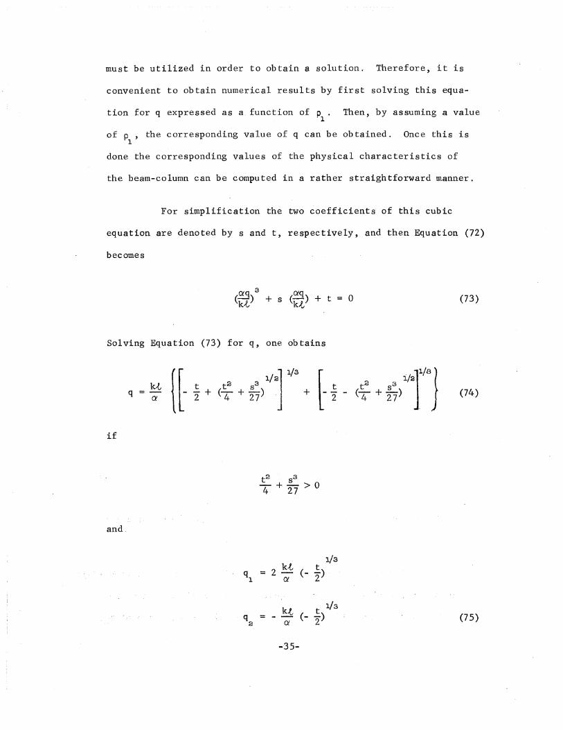
must be utilized in order to obtain a solution. Therefore, it is

convenient to obtain numerical results by first solving this equa-

tion for q expressed as a, function of p. Then, by assuming a value1

of p , the corresponding value of q can be obtained. Once this is1

done the corresponding values of the physical characteristics of

the beam-column can be computed in a rather straightforward manner.

For simplification the two coefficients of this cubic

equation are denoted by sand t, respectively, and then Equation (72)

becomes

(Q'q) + t+ s kt

Solving Equation (73) for q, one obtains

o (73)

ktq = a (74)

if

and.

2 kt1/3

tql = (- -)

a 2

k-t t 1/3(75)q = - - (- -)

2 Ci 2

-35-

if

and

2 kt1/2

'Ysq = (- -) cos '31 Q' 3

1/2

(1 + 120°)qa = 2 k-t (_ 2.) cos (76)Ci 3 3

2 kt S 1/2(-! + 240°)qa = (- -) cos

O! 3 3

if

in which ~ is defined as

cos 'l' - -

1/2t S~"2 / (- 27) (77)

in which sand t present themselves as functions of the parameter

p .1

For a given value of p "there will exist one (Equation (74»,1

two (Equation (75», or three (Equation (76» real roots for the

,lateral load q, possibly. -Each root of q will give a value of ~ .m

-36-

The values of q and ~ so obtained can either be positive or nega­m

tive. The negative sign of the value q indicates that q acts op-

posite to the direction assumed in Fig. 1, but can produce either

positive or negative curvature at the central portion of the beam-

column. However, if one consideres only the particular case of

positive q and positive ~ , then the solution for q, satisfyingm

such conditions, will be uni'que, and the unique value of q will be

given by q .1

Values of p . must lie between the limits .t/2 and p t2 ,2

(as yet undefined, pt > 0). The value t/2 corresponds to ~ = ~ ,2 - m 2

the value of q is given by Equation (64), and the corresponding

upper limit value of p is P u, 'which is, of course, equal to the1. 1

lower limit value of p t obtained already in Case 2. When the1

curvature ~ , as given by Equation (68), approaches infinity them

plastic regions in the upper and lower portions of the beam-column

meet at the center and a so-called plastic hinge forms, and the

value of q is

f 11

/

2

) --. ,epa

(77)

.tand the corresponding lower limit value, p ,of P , and therefore1 1

the lower limit value, Pat, can readily be found from Equation (72)

by trial and error.

Again, as discussed in Section 8, it is possible that

the end loadings may be large enough to cause part of the

-3-7-

beam-column to become plastic on two sides already before the lateral

load q is applied. In such circumstances the initial upper limit

value of p will he p 0 instead of the value t/2. The value of P1

o,

a 2

owhich corresponds to q = a (or p = p ), can be obtained from

a 2

Equation (72) by equating q to zero and by using a method of trial

and Values of must lie between the limits 0 and·error. P1now P1

p t and the values of must lie between 0and t The lateralPa Pa

p .1 a

load q corresponding to 0is zero. The load q correspondingP

1= P1

to P = P t is given by Equation (77). For other values of q Equa-l 1

tions (74), (75), and (76) can be used readily by assuming various

values of p .1

-38-

10. NUMERICAL RESULTS

Interaction Curves

A complete numerical evaluation of this solution for the

beam-column problem has been performed on a CDC 6400 Digital Com-

puter. The results of calculations made with various individual

cases are calculated for structural steel with E = 30,OOO·ksi and

cr = 34 ksi.y

The desired (q, ~ )-curve can be obtained directly fromm

various individual cases. A typical plot of q versus ~ for am

beam-column of given eccentricity ratio e/r and slenderness ratio

t/r, subjected to the constant load p, is shown in Fig. 6 in which

values of e/r = 1, tlr = 40, and p = 0.2, 0.4 have been used. The

small circles and the dotted lines in the figure indicate the dif-

ferent stages of plastification within the beam-column. It is

known that for any given axial force p it is necessary to increase

the lateral load q at the beginning in order to produce an increase

of mid-section curvature, while beyond a certain limit, given by

the maximum point of the curve, further curvature may proceed with

a diminishing of'the load. Although the diminishing of the load

with respect to an increase in curvature is not seen' for the curve

P =-0.2 (within the range of ~ less than 10) and is hot rapid for

the curve p = '0.4 as shown in Fig. 6, it is observed, however, that

wh-en'the slenderness ratio of the beam-column and/or the axial com-

pressive force are increased, there is a rapid diminishing portion

6£ 'the'-c't:frve beyond the maximum point. Thu's the maximum points of

-39-

the curves in Fig. 6 represent, for the given slenderness ratio and

assumed eccentricity, the maximum strength of the beam-column.

The maximum loads obtained in this way for various values

of axial force p, slenderness ratio tlr, and assumed ,eccentricity

ratio e/r are represented by the interaction curv~s in Figs. 7 to 10.

The curyes are drawn for values of tlr from 20 to 160 and each graph

is plotted for a value of elr and a particular cross section. For

each value of elr (0 and 0.5), two sets of such curves are 'shown,

one for R = 0 valid for a solid rectangular cross section, and the

other for R = 1.4, valid for a wide-flange cross section (8 W 31).

The dotted-open circle curves in Fig. 7 to Fig. 10 represent the

dividing lines between the range of applicability of various indi-

vidual cases. Each curve is for a particular beam-column and gives

the combinations of axial force and lateral load that can be safely

supported by the beam-column. Since the interaction curves are

nondimensionalized, they can be directly used in analysis and design

computations.

The intera,ct~on curves. de,termined by the analytical solu­

tions for an eccentri,cally loaded column are compared ~,n Fig. 11.

with those ob tained pr~viously by Galambos and Ketter [13,], usiJ;l.g the

method of num~_r.ical integration_. It can be seen that, in genera,l,

the values of the maximumlstr~ngth compu ted from t.he, appr_O,?imat.~

I '",. ._ " , .' _ . . ,', '

m-q>-p curve (Fig. 3), ,,:ts lower tha~ the ,?alues, determined from the

re~l m-~-p curve (exce~t th~ cu~ve t/r = 20 in the lower axial force

rang~), but_ t,he differ,~nce is usually small. This is exp~cte~ because• "."".; 4l :J. .• . I •

the approximate m-cp-p curves in Fig. 3 generally underestimate the

real curves. It-should be noted, however, that the interaction

curves of the present analytical solutions are based on 0.05 p

intervals while the curves obtained by numerical integration are

generally based on 0.2 p [13J. Therefore, part of the discrepancy

probably results from such difference in plotting.

It was shown in Section 4 that the generalized m-~-p

expressions generally tend to overestimate the actual momen-t when

the value of R is assumed to be. 1 (Fig. 4, ~ ~ 1~1) and to under­

estimate when the value of R is assumed to be 1.4 (Fig~ 3). Thus

the maximum loads of a beam~column computed from the value R = 1

will be an upper bound on the actual maximum load. The maximum

loads computed from R = 1.4 will be a lower bound. In Figs. 12

and 13 are shown two sets of interaction curves of this kind cal­

culated for e/r ~ 0, 0.5, respectively. It can be seen that the

interaction curves are relatively insensitive to minor variations

in R, especially for "hearn-columns with high slenderness ratio. It

may he concluded from this comparison that the i.nteraction curves

derived here for a particular value of R, 'far example R = 1.4, may

be used for the analysis of all wide-flange beam-column sections

(on conservative side for 8 W 31 section).

It was ,shown in Section 4 that for a give~ cross section

and a given axial force, the constants which specify the generalized

m-~-p relationship will be known from Equations (16) to (28).

-41-

Assuming that the axial force p is maintained at 'a constant value,

it can be seen from the solutions of the preceding sections that

the functional relationship between the lateral load q and the

mid-section curvature ~ only involves two independent parametersm

e/r (or m ) and kt. The parameter k~ is of importance in thea

analysis and design of beam-column, because it enables the inter-

action curves prepared for one yield stress level to be used for

different yield 'stress levels. Since the axial force p is assumed

to remain constant for a particular beam-column problem, the

par~eter kt becomes a function of the two ratios: cr IE and t/ry

kt = JP crY. (~) (78)E r

As long as the value for the parameter kt remains the same, the

(q, ~ )-curves corresponding to different combinations of cr IE andm ' y

tlr will be identical for any assumed eccentricity ratio. Thus the

interaction curves, prepared here for steel with a yield stress of

34 ksi, can be applied t~ steels of other yield~stress levels by

simply ,substituting, an equivalent ~lenderness ratio

, (79)

·Here E is assum~d to be the same for all different yield stress steels.

This conclusiQn is identical with that of Reference 14.

-42-

Initial Curvature

If an initially curved beam-column with an initial cur-

*vature ~o is submitted to the action of an axial force p and a

"1<distributed lateral load w(x), additional curvatures ~ will he

1

produced so that the final ordinates of the curvature curve are

* "1<ep = CPo + CPl (80)

and the equation of equilibrium for bending of the beam-column is,

in the usual notation

It can be seen that the differential equation for the cur-

*vature curve cp of the initially curved beam-column is of the same1.

form and has the same boundary conditions as that of a straight beam-

2 *column but with an additional lateral load k cp. Therefore, theo

problem of bending of an initially curved be~m-column can be approached

-43-

by the concept of replacing the effect of initial curvature .on the

curvature~ by th~ effect of an equivalent lateral load of the in-~k

tensity k2 ~. The dimensional form of the expression for the in­a

tensity of the equivalent lateral load is P ~o which is obtained by

i<multiplying the dimensionless value k2 ~o by My and using the

notation k2 p ~ 1M .y Y

In the previous discussions, one considered a very general

case of an inelastic beam-column with initial curvature and distri-

buted lateral load. The partic~lar case of an elastic column com-

pressed by force p applied at the ends has been discussed thoroughly

by Timoshenko [1J.

·As an exa~ple, assume that the initial shape of the beam-

column consists of two equal straight-line portions, as shown by

dotted line in Fig. 14, with a maximum deflection at the middl~ equal

to y. The equ.ivalent latera~" load becomes a concentrated load Q ato

the middle span. The magnitude of the equivalent lateral load is

obtained from the above expression

y ~

Q = J.f- P 91: dx = JP de: = 4P (z)o

(83)

*where e "denotes the. sl.ope of the initial shape of the beam-"column,o

or ,in nondimensional form the equivalent lateral load has the fbrrn

D h)2 (Y,o)q = (.L-) ,(~:20' r h

~44-

'. ,"(84)

Through the use of the equivalent lateral load concept,

the effect of this curvature on the maximum strength of a beam-

column can be readily obtained from the interaction curves similar

to those in Figs. 7 to 10. Since the ratio of the cross section

depth to the radius of gyration as well as the shape factor of a

cross section depend on the shape of the cross section, the above

equivalent lateral load will also depend on the shape of the cross

section. Take rectangular cross section, for example, the values

of h/r and a are 2;3 and 1.5, respectively. If t~e initial deflec-

tion ratio y /h of the beam-column is assumed to be 1/20, say, theno

the value of the equivalent lateral load, as given by Equation (84),

will be q = 0.2 p. The straight line q = 0.2 P is drawn in Fig. 7,

and the points of intersection of this line with the various inter-

action curves give the maximum s~rength of the column when it is

loaded with the specified initial curvature. The results obtained

are shown in Fig. 14 for several values of the initial curvature

y /h. The curve with the small circles in Fig. 14 are-plotted aso

corresponding small circles in Fig. 7 for the particular value of

y /h = 1/20.a

In column design it was pointed out [1J that it is logical

to assume that the initial curvature of a column may be compensated

for by a certain eccentricity in the application of the axial force.

In Fig. 15 three sets of such curves are compared, calculated for

a solid rectangular cross section. It is assumed that the values

-45-

of initial curvature are independent of the length of the column.

The comparison shows that the initial imperfections of a,column can

be compensated for with sufficient accuracy by a certain eccentricity.

Curvature Curves

The curvature curves obtained in the previous sections may

be plotted in a single diagram for various values of q. Figure 16

shows a family of such curves with e/r = 1, tlr = 60, and' p = 0.3.

The extent of the elastic, primary'plastic and secondary plastic

zones of the beam-column corresponding to different stages of load-

ing, q, are denoted by heavy solid lines, dotted lines) and light

solid lines, respectively, in the figure. These curves were com-

puted for beam-column with a rectangular cross section and again

with'material properties (J = 34 ksi and E = 30,000 ksi.y

Knowing the values of curvature along the elastic-plastic

beam-column, the lateral load vs. ~nd slope or the lateral load vs.

mid-span deflection can be readily obtained through the us~ of the

following two expressions

(J t2(EY) (-) 0.5 ~

ex=o = r_ S f- d (~)(~) 0 y,r

(85)

(J t 2

Yx=t/22(2) (r).· 0.5

(..!--)E S==h 2 ~h 0 y(--}r

(86)

-46-

As an example, taking the curvature curves as shown in

Fig. 16 as the basis for computations, the corresponding lateral

load vs. end slope curve is shown in Fig. 17 in which point 1 cor-

responds to the value of load q = 0.053 at which the yield point is

just reached in the most compressed fiber of the mid-section of the

beam-column; point 2 corresponds to the value of q = 0.292 for which

the fiber of maximum tensile stress of the mid-section on the convex

side of the beam-column has also reached its yield point, and the

maximum value of the curve for q is 0.371 which defines the maxi-

mum strength of the beam-column.

To see the rate of expansion of the plastic zones as the

end slope increases, the distances P1

and Pa which specify the

elastic-primary plastic boundary as well as the primary-secondary

plastic boundary, respectively, are also plotted against the end

slope in Fig. 17. It is seen that the initial rate of expansion

of the plastic zone on the compressive side of the beam-column (see

curve marked p ) is very rapid and this rate falls steadily, and1

the curve for P bends over more and more as the end slope increases1

When the end slope reaches the value approximately 0.,025 radians

the value of pbecomes practically a constant and equals the value].

0.093 t. The curve for p is very similar to the curve of p , but2 1

the initial rate ~f plastic expansion on the tensile side is less

rapid and the value of p practically approaches the constant 0.328 ~2

when the end slope reaches the value approximately 0.0275 radians.

-47-

From this discussion it can be concluded that when the

load q is gradually increased to its maximum and then drops off

steadily beyond the maximum point, the plastic zones spread first

toward the ends of the"bearn-column with a high initial rate of

expansion with respect to the rate of expansion toward the axis of

the beam-column. Beyond a certain value of q, further end rotation

may proceed with mainly expanding the plastic zones toward the axis

of the beam-column while the expansion toward the ends has practical­

ly ceased. In the limit the plastic regions in the upper and lower

portions of the beam-column will meet at the center and a so-called

plastic hinge forms.

, -'I,'

. \ ..

-48-

11. CONCLUSIONS

An analytical solution that describes the elastic-plastic

behavior of an eccentrically loaded beam-column u~der a concentrated

load at the mid-span was obtained. In the analysis, the moment­

curvature-thrust relationships derived previously for a rectangular

section are generalized to represent any complex shape of structural

section to a high degree of approximation. Furthermore, curvature

instead of deflection was utilized to simplify greatly the mathe­

matical aspect.of the problem. 'It is shown how the load-curvature

curves of beam-columns can be obtained directly from the solution.

The interaction curves for the applied lateral load versus axial

force with various values of slenderness ratio and eccentricity

ratio of the beam-column at the instant of collapse was obtained

from the load-curvature curves.

-49-

12 . ACKNOWLEDGEMENTS

The work is a part of the general investigation on "Space

Frames with Biaxial Loading in Columns", currently being carried out

at the Fritz Engineering Laboratory, Lehigh University. This study

is sponsored jointly by the Welding Research Council and the Depart­

ment of the Navy, with funds furnished by the American Iron and Steel

Institute, Naval Ships System Command, and Naval Facilities Engineering

Command.

Technical advice for the project is provided by the Lehigh

Proje9t Subcommittee of the Structural Steel Committee of the Welding

Research Council, of which T. R. Higgins is Chairman.

The writer wishes to acknowledge S. N. Iyengar for his

help in computer programming, to L. W. Lu and G. C. Driscoll for

their review of the manuscript, to J. Lenner for her help in typing

the manuscript, and to J. Gera for preparing the drawings.

,-50-

13. FIGURES

-51-

1-y

Q

......-p x

..ICase I

(a) Elastic

P

ElasticZone

PrimaryPlasticZone

Q

ElasticZone

P

y Case 2

P

yCase 3

(b) One Side Plastic

P x

Fig. '1 Eccentrically Loaded Beam-Column

-52-

SecondaryPrimary Plastic Primary

Elast~ l~asti.;'I1"n!.l~ast!:I~.ast~1t10 e Zone Q. Z Zone

...-...-p xP

y Case 4

P P x

y Case 5

p x

Iy Case -6

(c) Two- Side Plastic

Fig. 1 Eccentrically Loaded Beam-Column (Contd.)

-53-

PrimaryPlastic

m

IIII

- II

ElasticII

SecondaryPlastic

Fig. 2 Moment-Curvature-Thrust Relationship for aCommon Structural Section

. }".

-54-

1.0p=0.2

5

p =0.8

432_. I-0

0.4

0.8 p =0.4

MMY

0.6p= 0~6

.Fig.3 Moment-Curvature-Thrust Relationships(Ac~u·al·Curves, Shown Dashed)

_~55-

1.0

M-My

0.5

o ··-1.0

., ~.. :, ~~ ·...·a·_·.~

p= 0.2

----------

-_ ..........---- ,,'

p =0.6

p=O.8'------", ~ i

--R=I., ~'

., t

---.- 8YF31

2.0

j·'F.ig~ 4 'Moment-Curvattire~Thrust Relationships,1"- ,{. (Actual 'CurV'es:i SI10wd Dashed)

'~56-

Y (0) Beam· - Column

(b) Nondim~nsional Curvature Curve

Moment due". to load Q

Moment due to Deflection

(c) Nondimensional Moment Diagram

Fig. 5 Discontinuities 'in the Derivative ofthe Curvature Curve

-57-

Q!4My

1.0

0.8

o....(1)

ca::Q)

:2.~ CJ)

1;;­c CD- c:LaJo

o+=enca:.Q)

-c.-(f)

Io~I-

R=O (Rectangle)

~ =0.2y

I it.1 -'I"·

"

',- 1

0.6

0.4

0.2

o

•. :... ','J

2 4

lo .• ~~. I ~ -..... _~ - • \ ~:.

Case 4

C,ase,5,

6

;;=0.4y

8 10

. -'. ,. ': :- "',' ':. :', -' f " ~ " -, l,'-' ,l -, ,.' .'- ':~ , ::. "" ", - ,,', i,.-~ .', .'-'" 'Fig:>:"6" Lat e't-':a l' Load vs~ 'Mid-Section Curvature

Curves. E = 30,OOQ~Ei,·cr = 34 ksi~ , ':.' . y ,,'

;~,58-

1.00.5

Q-'Qp

o

1.0 .....-----------..----------Q--------.

+p --.t-----,l........--J4-P

R= 0(Rectangle)E=30,000 ksitry=34 ksi

2040

0.5

pPy

," Fig'. 7 Interaction Curves for -a RectangularCrqss Section

1.0

R= 1.4(SW-31)

E= 30,OOOksitTy =34 ksi

0.5

Q-Qp

+Qp --o----.......---o..... p

~ ~ -I

2040

6080

100

120140

,t _160T-

o

1.0

0.5

F,ig. 8 Interact,ion Curves for a Wide-FlangeCross Section

-60-

1.0--------------0---

2---..

pI __k__

~ )f ..1J,.5rp-Py

0.5

o

R=O( Rectangle)

E= 30,000 ksioy= 34 ksi

20=1-40

0.5

Q-Q p

Fig. 9 Interaction Cruves for a Rectangular CrossS~ctio~cwith a.Constant Eccentricity

-61-

1.0

1.0--------------------,

p- 0.5Py

R'= 1.4(8YF31)E= 30,000ksi0;= 34 ksi

0 0.5 1.0

Q-Qp

Fig.- 10 Interaction-Curves for a Wide-Flange CrossSection with a Constant Eccentricity

-62-

1.00.5o

1.0

~P; h)(.1

~ ~l.E.

Present Sol. (R=1.4)Py0 Ref. 13 Sol.

E=30,000 ksi

20uy=34 ksi

8YF31

0.5

Fig. 11 Compari'son Between IIAnalytical tI and"Numerical" Interaction Curves

... 63-

1.0

~--i-Q--o......-p~ -I ·

0.5

: Q"." ..--- '.(

Qp")'

,J-:r

o

I .o..........------....-.------~---,

0.5

p

15Y

Fig. 12 Comparison of Lower and Upper Boundsfor tbe Ul,tim.ate ,Str.ength~,;0£ an, 'Ax'ia'l,ly':' 'Lo~flP,ed ,',Beam-'Col'uinn

, ~'- '

-64-

1.0....------------..;-...-....------------,

P1__t_Q_oP1_ ,I _le=0.5r

---R = 1.0-R= 1.4

E=30,~OO ksiay =34 ksi

0 0.5 1.0

Q-

Q .p

-·Fig. 13 Co~paiison of L6~er and Upper Bounds for theUltimate Strength of an Eccentricity Loaded

Beam-Column

-65-

-2

-9 I

E= 30,000 ksioy= 34 ksiR= 0( Rectangle)

I4

ITO

Euler Hyperbola~\\\\\\\

~I

1.0

0.5

o 100

1r

200

Fig. 14 The Effect of Initial Curvature on the"'\, Ultimate Strength.o,f a Column

-66-

1.0

0.5

r

R= 0(Rectangle)E=30,000 ksioy= 34 ksi

100

-l-r

200

Fig. 15 Comparison of Column Curves for a Column with. In~tial Im~erfections an~. for a Column

~it~ Initial" End Eccentricities

--67-

10

8

4>('!") 61

4

2

o 0.1 0.2

q= 0.352

xJ.

,Rectangular Section

-Elastic--- Primary Plastic

-Secondary Plastic

..!...= IrJ.-=60r

P -- -0.3Py

U'y =34 ksi

E =30,000 ksi

0.7 0.8'0.9 1.0

_: ~ , .j

cu-~v~'tti;re,~~, 'a,iong- the Length of a,-".,,' 2 '" .' B-eam':'Co!umn '

'--68-

0.4....!L =I· 1=60 L=0.3 Rectangular Section

r r Py

0.3

0.5

Q- 0.2 P2 0.4-Q p

0.3 P P.....Lor.A

0.1 0.2 '1 1.PI

o. I

0.010 .015 .020 .025 .030 .035

8x=o (RADIANS)

Fig. 17 Lateral Load vs. End Slope Curve. and theCorresponding Values for P

1and P

a

-69-

APPENDICES

14. APPENDIX I - SOLUTION FOR CASE 3, CASE- 5, AND CASE 6

Case 3 [Fig. l(b)] - The-general solution of the curvature curve of

this case is given by Equation (37). The constant D is found from

the condition tha,t dcp/dx in Equation (34) must satisfy the "jump

condition", as given by Equation (49). Hence

1/2 + _2 rvq 2D = cp (-~-) (87)

m c kt

, The constant x and the unknown quantity ~ can be determined fromp m

the conditions that ~ in Equation (37) must equal ~ and ~ form 0

x = ~/2·and x = 0, respectively. One obtatns

xII 1 f aq 1 Ie 1. 1 [12 1 ~}--E. = - + - - (ko.) ----va + - l'2 tanh- -'~ (~):.._'t 2 D kt 'V cp "1'" 12 D"t~1c D7~ kt

m

(88)

and the desired equation'for the detenmination .of the unknown cur-

where

-70-

valid for

qJo(b-m )2

o

(90)

and

Case 5 [Fig. l(c)] - The derivatives of tha curvature function for

the primary plastic zone and for the secondary plastic zone are given

by Equation (34) and Equation (35), respectively. The constants D

and G are found from the jump condition, as given by Equation (50),

for the central cross section where the concentrated load is applied,

and also the jump condition, as given by Equation (45), for the sec-

tion where the primary plastic zone and secondary plastic zone meet.

Using the fact that ~x=-t/2 = ~m' and ~x=p2

that

= ~ , it can be concluded2

2G 1 (O!q) 1

= f kt rnTm

-, ,,,71-

(91)

To determine the curvature curve in the secondary plastic

zone, the constant x in Equation (38) and the unknown distance ps 2

must be determined. The values x and p are found from the conditionss 2

that ~, as given by Equation (38), must equal ~2 for x = Pa

and must

equal ~ for x = t/2, respectively. One obtainsm

and

X s 1 2(Q'q)

T = "2 - kt ,kt (92)

Pa ~ {f f! 2 r/2

[

(aq)2]1 (GYq) +.1.. " ~. 1 1 " 2 2- = -- -- - +- - ft 2 3 kt f kt ~2 cp~ '.' tpa Ci'm kt

+ 2.. (aq) [1- '2 (aq)2] (93)

l<.t kt ep 3f kt ... ' , m

To determine the curvature curve in the primary plastic

zone, the constant x in Equation, (37) and the unknown quantity ~p c m

must be determined. The values x and ~ are found from the con­pm.

ditions that ~, as given by Equati~n (37), must equal ~o for x = 0

and must equal cp for x = p ,respectively. One obtains2 :3

.,/ .1/2J.f2 '

(D-~ )o 1 . 1

+ 112 tanh­D

(94)

in which cp is given by ~quation (90) and the desired equation foro

the unknown curvature ~ at the central cross section of the beam­m

column

(95)

1/2)1/2_1 CP2 t'- tanh (1 --n-

_l ( CPoJ/2)1/2tanh 1 - -n-.

1+~

D

/ 1/21 2

Q:'q [1 2 Q:'q 2] IC 1{(D-qJ0 )- 2 (k,e) cp - 3£ (k,e,) + -, D 1/2

m 12 cpo

1/2 1/2(D-cp )

2

valid for

and

It is seen that the constants D, G, x , x , and the dis­s p

tance, p , all present themselves as a function of the central cross1

section curvature ~ , for a given beam-column. Since rn > to , it ism T m - "2

convenient to obtain numerical results by first assuming a value of

~m and obtaining the corresponding value of q from Equation (95) by

trial and error. Once this is done, the corresponding values of the

physical characteristics of the beam-column can be computed in a

straightforward manner. Case 3 and Case 6 can be treated in a similar

manner.

'-73-

Case 6 -[~i'g. 1 (c) J ~ The' general~olution of the c~rvature curve of

this case is given by Equation (38). The constants G and x ins

Equation (38) are given by Equation (91) and ~quation (92), respective-

lYe The value of e.p can be determined from the equationm

3 Q<l [ 2 . aq 2 . 3] IL [ 1 1- lvf., = (-) - (-) .. -. + vI - - -4 kt f k.t cp - cp CP,mom

+ 1. (O!Q)2]1/2

[1 + 2 ~ (~)2]f kt ~o ~m - f

(96)

where

(97)

valid for

c.p < cp:3 ~- 0

and

., --74-

15. APPENDIX II - SAMPLE CURVES

"-75-

1.00.5

Q-Qp

o

1.0-----------------Q------,

p ---,........_t......· ...............~pI- )! J~OOlr

R=O( Rectangle)E=30, 000 ksiO"y=34 ksi

0.5

Fig. 18 Interaction Curves for a Rectangular CrossSection with an End Eccentricity

~ 7-6-

1.0

P-.....I __tQ r..J p

I.. ,t ..IJolrR=O( Rectangle)E= 30,000 ksiO"y=34 ksi

o

I.O~-----------------------'

0.5

p-Py

lriteract:ion Curves.f~~" a Rectangular CrossSection with 'an End Eccentricity

,-:-:77-

1.0

0.5

o

R=O( Rectangle)E= 30,000 ksiU'y= 34 .ksi

0.5

Q---Qp

. F:i;g. 20. Int.eras.ti.o.n Curves for a Rect~ngular Cross, '" " 'sec't~o~, ~it~·'aJ.1. '"End Eccentricity

:"'78-

1.0

1.0 ,<

-'-=r

o

1.0

I,Q 2p

~. ~ ~J;.lrp

Py R=O(Rectangle)E= 30,000 ksiuy=34 ksi

0.5

Fig~ 21'. Interaction Curves for a RectangQlar Cross,~" ,J. Sectirin with ari tnd~Ecc~nt~iciity

~ L • l.: •

. -,79-

1.0

PI tQ 2p

~ ~ -IJrP R'=OPy ( RectangIe )

E=30, 000 k~i

oy= 34 ksi

0.5

0 0.5 1.0

Q-Qp

~~ge. 22 .. Int~ra6~~on CU~Y~~ for ~ Rectan~~lar CrossSection with 'an End Eccentricity

-":80-

1.0

*Q ~PP~

~f,I. ..le:2r

P R=O-Py ( Rectangle)E= 30,000 ksiuy=34 ksi

0.5

° 0.5

Q-Q p

Fig. 23 Interaction Curves for a Rectangular CrossSection 'with an End Eccel}tricity

-81-

1.0

f.0..-----------------------

0.5

o

~ ---r

0.5

QQp

R= 1.4(8YF31)E=30, 000 ksicry =34 ksi

1.0

Fig. ;24 Iriteraction C~rves for a Wide-Flange Sectionwith an End Eccentricity-

-82-

: 1.0 ..---------------------.

p-Py

0.5

R= 1.4(8 W- 31)

E= 30,000 ksi

cry :: 34 ksi

'l, i,

0 0.5 1.0

Q-Qp

Fig. 25 Int~~~~f!6~ Cur~e~ f6r'a Wide-Flange Sectionwith an End Eccentricity

1.0--------------------,

R-I.4(SVF31)

E=30,000 kli

cr =34ksiy

o 0.5

Q

'Q p

2040

60----"""80,

100120

140160

0.5

Fig. 26 Interaction Curves for a Wide-Flange Sectionwith an En~ Eccen~ricity

-84-

1.0---------------------.

R= 1.4(8VF31)E=30,000ksi

0;= 34 ksi0.5

o

i:-

r

Case 4

0.5

Q-'Qp

Fig.J

27 Interaction Curves for a Wide-Flange Sectionwith an End Eccentricity

-85~>

o

16. NOTATION

A = area of section

A ,B,D,G,x ,x = constants of integration1 p s

a,b,c,f,m ,m ,m ,~,~ = arbitrary constants define the1 2 pc 1 2

generalized m-~-p curve

E

e

h

I

k

M

Mo

MY

m

mo

p

py

p

Q

= modulus of elasticity

= eccentricity

= depth of section

moment of inertia of section about

the axis of bending

= '/P lEI

= length of beam-column

= be~ding moment

= applied moment at the end of beam-'

column

moment which causes first yielding

in the s~c,tion

= M/MY

= M 1Mo y

= thrust

= axial yield load

= pipy

= concentrated lateral load

= plastic limit load according to

simple plastic theory

q

ql,q ,q2 3

R

r

s

x,Y

= Q/Qp

= roots of the cubic Equation (72)

= section variable

= radius of gyration about the axis

of bending

= elastic section modulus

= coordinate axes

= shape factor of section about the

axis of bending

= strain at yield point

distance from the end to the primary

plastic zone of the beam-column

= distance from the end to the secondary

plastic zone of the beam-column

function defined in Equation (60)

= yi-eld stress

= curvature

~ initial curvature

= mid-span curvature

= curvature at initial yielding for

pure bending moment

= ~/~y

= ~ /~m y

-87_~

17. REFERENCES

1. Timoshenko, s. P. and Gere, J. M.THEORY OF ELASTIC STABILITY, 2nd Edition, McGraw-Hill BookCo., Inc., New York, 1961.

2. Chen, w. F~ and Santathadaporn, s.CURVATURE AND THE SOLUTION OF ECCENTRICALLY LOADED COLUMNS,Journal of the Engineering Mechanics Division, ASCE,Vol. 95, No. EMl, February 1969.

3. Hauck, G. F. and Lee, S. L.STABILITY OF ELASTO-PLASTIC WIDE-FLANGE COLUMNS, Journalof the Structural Division, ASeE, Vol. 89, No. ST6,Prac. Paper 3738, pp. 297-324, December 1963.

4. Wright, D. T.THE DESIGN OF COMPRESSED BEAMS, The Engineering Journal,Canada, Vol. 39, p. 127, February 1956.

5. Ketter, R. L.FURTHER STUDIES ON THE STRENGTH OF BEAM-COLUMNS, Journalof the Structural Division, ASeE, Vol. 87, No. 8T6, Proc.Paper 2910, p. 135, August 1961.

6. Horne, M. R. and Merchant, WTHE STABILlr;N OF FRAMES, Pergamon Press, Inc., New York1965.

7. Lu, L. W. and Kama1vand, H.ULTmATE STRENGTH OF LATERALLY LOADED COLUMNS, Journal ofthe Structural Division, ASCE, Vol. 94, No. ST6, pp. 1505­1523, June 1968.

8. Von Karman, T.UNTERSUCHUNGEN UBER KNICKFESTIGKEIT, Mitteilungen UberForschungsarbeiten, Herausgegeben Vorn Verein DeutscherIngenieure, No. 81, Berlin, 1910.

9. Chwalla, E.AUSSERMITTIG GEDRUCKTE BAUSTAHLSTABE MIT ELASTISCHEINGESPANNTEN ENDEN UND VERSCHIEDEN GROSSEN ANGRIFFSH~BELN,

Der Stah1bau, Vol. 15, Nos. 7 and 8, pp. 49 and 57, 1937.

10. Ojalvo, M..RESTRAINED COLUMNS, Proe. ASCE" Vol. 86 (EM.5), p. l, 1960.

11. Baker, J. F., Horne, M. R., and Roderick, J. W.THE BEHAVIOR OF CONTINUOUS STANCHIONS, Proe. of RoyalSociety, Serial A, Vol. 198, p. 493, 1949.

-88"-"

12. Ketter, K. L., Kaminsky, E. L., and Beedle, L. S.PLASTIC DEFORMATION OF WIDE-FLANGE BEAM-COLUMNS, Trans.ASCE, Vol. 120, p. 1028, 1955.

13. Galambos, T. V. and Ketter, R. L.FURTHER STUDIES OF COLUMNS UNDER COMB INED BENDING ANDTHRUST, Fritz Laboratory Report No. 205A.19, LehighUniversity, June 1957.

14. Column Research CouncilGUIDE TO DESIGN CRITERIA FOR METAL COMPRESSION MEMBERS,Chapter 6, Edited by B. G. Johnston, John Wiley andSons, Inc., New York, 1966.

-89-