generalization of the levinson inequality with...

Adeel et al. Journal of Inequalities and Applications (2019) 2019:230 https://doi.org/10.1186/s13660-019-2186-4

R E S E A R C H Open Access

Generalization of the Levinson inequalitywith applications to information theoryMuhammad Adeel1*, Khuram Ali Khan1, Ðilda Pecaric2 and Josip Pecaric3

*Correspondence:[email protected] of Mathematics,University of Sargodha, Sargodha,PakistanFull list of author information isavailable at the end of the article

AbstractIn the presented paper, Levinson’s inequality for the 3-convex function is generalizedby using two Green functions. Cebyšev-, Grüss- and Ostrowski-type new bounds arefound for the functionals involving data points of two types. Moreover, the mainresults are applied to information theory via the f -divergence, the Rényi divergence,the Rényi entropy, the Shannon entropy and the Zipf–Mandelbrot law.

Keywords: Levinson’s inequality; Information theory

1 Introduction and preliminariesIn [12], Ky Fan’s inequality is generalized by Levinson for 3-convex functions as follows.

Theorem A Let f : I = (0, 2α) →R with f (3)(t) ≥ 0. Let xk ∈ (0,α) and pk > 0. Then

J1(f ) ≥ 0, (1)

where

J1(f (·)) =

1Pn

n∑

ρ=1

pρ f (2α – xρ) – f

(1

Pn

n∑

ρ=1

pρ(2α – xρ)

)

–1

Pn

n∑

ρ=1

pρ f (xρ)

+ f

(1

Pn

n∑

ρ=1

pρxρ

)

. (2)

Working with the various differences, the assumptions of differentiability on f can be weak-ened.

In [18], Popoviciu noted that (1) is valid on (0, 2a) for 3-convex functions, while in [2],Bullen gave a different proof of Popoviciu’s result and also the converse of (1).

Theorem B(a) Let f : I = [a, b] →R be a 3-convex function and xn, yn ∈ [a, b] for n = 1, 2, . . . , k such

that

max{x1 . . . xk} ≤ min{y1 . . . yk}, x1 + y1 = · · · = xk + yk , (3)

© The Author(s) 2019. This article is distributed under the terms of the Creative Commons Attribution 4.0 International License(http://creativecommons.org/licenses/by/4.0/), which permits unrestricted use, distribution, and reproduction in anymedium, pro-vided you give appropriate credit to the original author(s) and the source, provide a link to the Creative Commons license, andindicate if changes were made.

https://doi.org/10.1186/s13660-019-2186-4

http://crossmark.crossref.org/dialog/?doi=10.1186/s13660-019-2186-4&domain=pdf

mailto:[email protected]

Adeel et al. Journal of Inequalities and Applications (2019) 2019:230 of 18

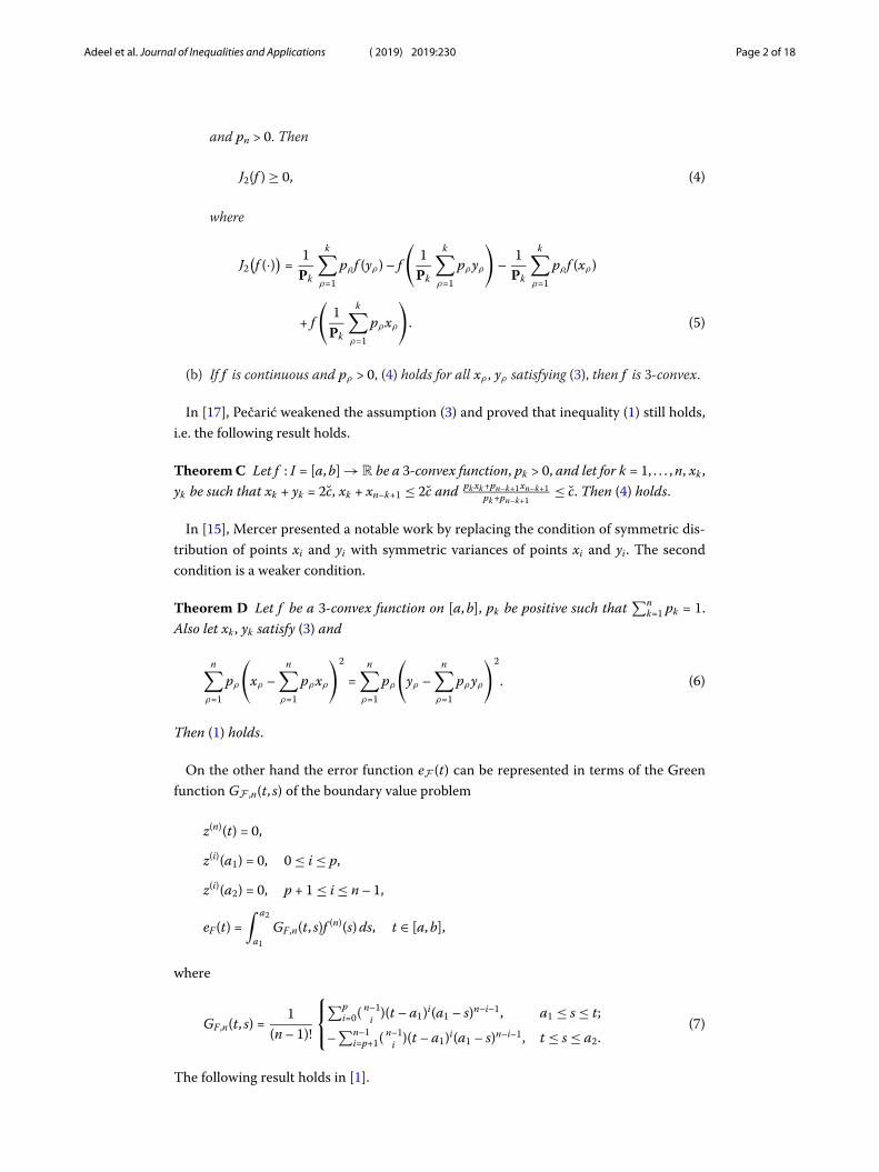
and pn > 0. Then

J2(f ) ≥ 0, (4)

where

J2(f (·)) =

1Pk

k∑

ρ=1

pρ f (yρ) – f

(1

Pk

k∑

ρ=1

pρyρ

)

–1

Pk

k∑

ρ=1

pρ f (xρ)

+ f

(1

Pk

k∑

ρ=1

pρxρ

)

. (5)

(b) If f is continuous and pρ > 0, (4) holds for all xρ , yρ satisfying (3), then f is 3-convex.

In [17], Pečarić weakened the assumption (3) and proved that inequality (1) still holds,i.e. the following result holds.

Theorem C Let f : I = [a, b] →R be a 3-convex function, pk > 0, and let for k = 1, . . . , n, xk ,yk be such that xk + yk = 2c, xk + xn–k+1 ≤ 2c and pk xk +pn–k+1xn–k+1

pk +pn–k+1≤ c. Then (4) holds.

In [15], Mercer presented a notable work by replacing the condition of symmetric dis-tribution of points xi and yi with symmetric variances of points xi and yi. The secondcondition is a weaker condition.

Theorem D Let f be a 3-convex function on [a, b], pk be positive such that∑n

k=1 pk = 1.Also let xk , yk satisfy (3) and

n∑

ρ=1

pρ

(

xρ –n∑

ρ=1

pρxρ

)2

=n∑

ρ=1

pρ

(

yρ –n∑

ρ=1

pρyρ

)2

. (6)

Then (1) holds.

On the other hand the error function eF (t) can be represented in terms of the Greenfunction GF ,n(t, s) of the boundary value problem

z(n)(t) = 0,

z(i)(a1) = 0, 0 ≤ i ≤ p,

z(i)(a2) = 0, p + 1 ≤ i ≤ n – 1,

eF (t) =∫ a2

a1

GF ,n(t, s)f (n)(s) ds, t ∈ [a, b],

where

GF ,n(t, s) =1

(n – 1)!

⎧⎨

⎩

∑pi=0( n–1

i )(t – a1)i(a1 – s)n–i–1, a1 ≤ s ≤ t;

–∑n–1

i=p+1( n–1i )(t – a1)i(a1 – s)n–i–1, t ≤ s ≤ a2.

(7)

The following result holds in [1].


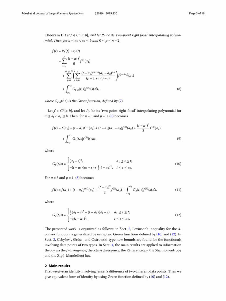
Theorem E Let f ∈ Cn[a, b], and let PF be its ‘two-point right focal’ interpolating polyno-mial. Then, for a ≤ a1 < a2 ≤ b and 0 ≤ p ≤ n – 2,

f (t) = PF (t) + eF (t)

=p∑

i=0

(t – a1)i

i!f (i)(a1)

+n–p–2∑

j=0

( j∑

i=0

(t – a1)p+1+i(a1 – a2)j–i

(p + 1 + i)!(j – i)!

)

f (p+1+j)(a2)

+∫ a2

a1

GF ,n(t, s)f (n)(s) ds, (8)

where GF ,n(t, s) is the Green function, defined by (7).

Let f ∈ Cn[a, b], and let PF be its ‘two-point right focal’ interpolating polynomial fora ≤ a1 < a2 ≤ b. Then, for n = 3 and p = 0, (8) becomes

f (t) = f (a1) + (t – a1)f (1)(a2) + (t – a1)(a1 – a2)f (2)(a2) +(t – a1)2

2f (2)(a2)

+∫ a2

a1

G1(t, s)f (3)(s) ds, (9)

where

G1(t, s) =

⎧⎨

⎩(a1 – s)2, a1 ≤ s ≤ t;

–(t – a1)(a1 – s) + 12 (t – a1)2, t ≤ s ≤ a2.

(10)

For n = 3 and p = 1, (8) becomes

f (t) = f (a1) + (t – a1)f (1)(a2) +(t – a1)2

2f (2)(a2) +

∫ a2

a1

G2(t, s)f (3)(s) ds, (11)

where

G2(t, s) =

⎧⎨

⎩

12 (a1 – s)2 + (t – a1)(a1 – s), a1 ≤ s ≤ t;

– 12 (t – a1)2, t ≤ s ≤ a2.

(12)

The presented work is organized as follows: in Sect. 2, Levinson’s inequality for the 3-convex function is generalized by using two Green functions defined by (10) and (12). InSect. 3, Čebyšev-, Grüss- and Ostrowski-type new bounds are found for the functionalsinvolving data points of two types. In Sect. 4, the main results are applied to informationtheory via the f -divergence, the Rényi divergence, the Rényi entropy, the Shannon entropyand the Zipf–Mandelbrot law.

2 Main resultsFirst we give an identity involving Jensen’s difference of two different data points. Then wegive equivalent form of identity by using Green function defined by (10) and (12).


Theorem 1 Let f ∈ C3[ζ1, ζ2] such that f : I = [ζ1, ζ2] → R, (p1, . . . , pn) ∈ Rn, (q1, . . . , qm) ∈

Rm such that

∑nρ=1 pρ = 1 and

∑m�=1 q� = 1. Also let xρ , y� ,

∑nρ=1 pρxρ ,

∑m�=1 q�y� ∈ I . Then

J(f (·)) =

12

[ m∑

�=1

q�y2� –

( m∑

�=1

q�y�

)2

–n∑

ρ=1

pρx2ρ +

( m∑

ρ=1

pρxρ

)2]

f (2)(ζ2)

+∫ ζ2

ζ1

J(Gk(·, s)

)f (3)(s) ds, (13)

where

J(f (·)) =

m∑

�=1

q�f (y�) – f

( m∑

�=1

q�y�

)

–n∑

ρ=1

pρ f (xρ) + f

( n∑

ρ=1

pρxρ

)

(14)

and

J(Gk(·, s)

)=

m∑

�=1

q�Gk(y�, s) – Gk

( m∑

�=1

q�y� , s

)

–n∑

ρ=1

pρGk(xρ , s) + Gk

( n∑

ρ=1

pρxρ , s

)

,

(15)

for Gk(·, s) (k = 1, 2) defined in (10) and (12), respectively.

Proof (i) For k = 1.Using (9) in (14), we have

J(f (·)) =

m∑

�=1

q�

[f (ζ1) + (y� – ζ1)f (1)(ζ2) + (y� – ζ1)(ζ1 – ζ2)f (2)(ζ2)

+(y� – ζ1)2

2f (2)(ζ2) +

∫ ζ2

ζ1

G1(y� , s)f (3)(s) ds]

–

[

f (ζ1) +

( m∑

�=1

q�y� – ζ1

)

f (1)(ζ2) +

( m∑

�=1

q�y� – ζ1

)

(ζ1 – ζ2)f (2)(ζ2)

+(∑m

�=1 q�y� – ζ1)2

2f (2)(ζ2) +

∫ ζ2

ζ1

G1

( m∑

�=1

q�y� , s

)

f (3)(s) ds

]

–n∑

ρ=1

pρ

[f (ζ1) + (xρ – ζ1)f (1)(ζ2) + (xρ – ζ1)(ζ1 – ζ2)f (2)(ζ2)

+(xρ – ζ1)2

2f (2)(ζ2) +

∫ ζ2

ζ1

G1(xρ , s)f (3)(s) ds]

+

[

f (ζ1) +

( n∑

ρ=1

pρxρ – ζ1

)

f (1)(ζ2) +

( n∑

ρ=1

pρxρ – ζ1

)

(ζ1 – ζ2)f (2)(ζ2)

+(∑n

ρ=1 pρxρ – ζ1)2

2f (2)(ζ2) +

∫ ζ2

ζ1

G1

( n∑

ρ=1

pρxρ , s

)

f (3)(s) ds

]

,


J(f (·)) = f (ζ1) +

( m∑

�=1

q�y� – ζ1

)

f (1)(ζ2) +

( m∑

�=1

q�y� – ζ1

)

(ζ1 – ζ2)f (2)(ζ2)

+(∑m

�=1 q�y2� – 2ζ1

∑m�=1 q�y� + ζ 2

1 )f (2)(ζ2)2

+m∑

i=1

q�

∫ ζ2

ζ1

G1(y�, s)f (3)(s) ds

– f (ζ1) –

( m∑

�=1

q�y� – ζ1

)

f (1)(ζ2) –

( m∑

�=1

q�y� – ζ1

)

(ζ1 – ζ2)f (2)(ζ2)

–((∑m

�=1 q�y�)2 – 2ζ1∑m

�=1 q�y� + ζ 21 )f (2)(ζ2)

2

–∫ ζ2

ζ1

G1

( m∑

�=1

q�y� , s

)

f (3)(s) ds

– f (ζ1) –

( n∑

ρ=1

pρxρ – ζ1

)

f (1)(ζ2) –

( n∑

ρ=1

pρxρ – ζ1

)

(ζ1 – ζ2)f (2)(ζ2)

–(∑n

ρ=1 pρx2ρ – 2ζ1

∑nρ=1 pρxρ + ζ 2

1 )f (2)(ζ2)2

–n∑

ρ=1

pρ

∫ ζ2

ζ1

G1(xρ , s)f (3)(s) ds

+ f (ζ1) +

( n∑

ρ=1

pρxρ – ζ1

)

f (1)(ζ2) +

( n∑

ρ=1

pρxρ – ζ1

)

(ζ1 – ζ2)f (2)(ζ2)

+((∑n

ρ=1 pρxρ)2 – 2ζ1∑n

ρ=1 pρxρ + ζ 21 )f (2)(ζ2)

2

+∫ ζ2

ζ1

G1

( n∑

ρ=1

pρxρ , s

)

f (3)(s) ds,

J(f (·)) =

12

[ m∑

�=1

q�y2� –

( m∑

�=1

q�y�

)2

–n∑

ρ=1

pρx2ρ +

( n∑

ρ=1

pρxρ

)2]

f (2)(ζ2)

+m∑

�=1

q�

∫ ζ2

ζ1

G1(y�, s)f (3)(s) ds –∫ ζ2

ζ1

G1

( m∑

�=1

q�y� , s

)

f (3)(s) ds

–n∑

ρ=1

pρ

∫ ζ2

ζ1

G1(xρ , s)f (3)(s) ds +∫ ζ2

ζ1

G1

( n∑

ρ=1

pρxρ , s

)

f (3)(s) ds.

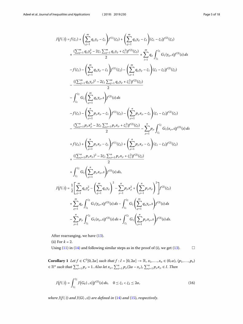
After rearranging, we have (13).(ii) For k = 2.Using (11) in (14) and following similar steps as in the proof of (i), we get (13). �

Corollary 1 Let f ∈ C3[0, 2α] such that f : I = [0, 2α] → R, x1, . . . , xn ∈ (0,α), (p1, . . . , pn)∈R

n such that∑n

ρ=1 pρ = 1. Also let xρ ,∑n

ρ=1 pρ(2α – xρ),∑n

ρ=1 pρxρ ∈ I . Then

J(f (·)) =

∫ ζ2

ζ1

J(Gk(·, s)

)f (3)(s) ds, 0 ≤ ζ1 < ζ2 ≤ 2α, (16)

where J(f (·)) and J(G(·, s)) are defined in (14) and (15), respectively.


Proof Choosing I = [0, 2α], y� = (2α – xρ), x1, . . . , xn ∈ (0,α), pρ = q� and m = n, in Theo-rem 1, after simplification we get (16). �

Theorem 2 Let f : I = [ζ1, ζ2] → R be a 3-convex function. Also let (p1, . . . , pn) ∈ Rn,

(q1, . . . , qm) ∈ Rm be such that


∑m�=1 q� = 1 and xρ , y� ,

∑nρ=1 pρxρ ,

∑m�=1 q�y� ∈ I .If

[ m∑

�=1

q�y2� –

( m∑

�=1

q�y�

)2

–n∑

ρ=1

pρx2ρ +

( n∑

ρ=1

pρxρ

)2]

f (2)(ζ2) ≥ 0, (17)

then the following statements are equivalent:For f ∈ C3[ζ1, ζ2]

n∑

ρ=1

pρ f (xρ) – f

( n∑

ρ=1

pρxρ

)

≤m∑

�=1

q�f (y�) – f

( m∑

�=1

q�y�

)

. (18)

For all s ∈ I

n∑

ρ=1

pρGk(xρ , s) – Gk

( n∑

ρ=1

pρxρ , s

)

≤m∑

�=1

q�Gk(y�, s) – Gk

( m∑

�=1

q�y� , s

)

, (19)

where Gk(·, s) are defined by (10) and (12) for k = 1, 2, respectively.

Proof (18) ⇒ (19): Let (18) is valid. Then as the function Gk(·, s) (s ∈ I) is also continuousand 3-convex, it follows that also for this function (18) holds, i.e. (19) is valid.

(19) ⇒ (18): If f is 3-convex, then without loss of generality, we can suppose that thereexists the third derivative of f . Let f ∈ C3[ζ1, ζ2] be a 3-convex function and (19) holds.Then we can represent the function f in the form (9). Now by means of some simplecalculations we can write

m∑

�=1

q�f (y�) – f

( m∑

�=1

q�y�

)

–n∑

ρ=1

pρ f (xρ) + f

( n∑

ρ=1

pρxρ

)

=12

[ m∑

�=1

q�y2� –

( m∑

�=1

q�y�

)2

–n∑

ρ=1

pρx2ρ +

( n∑

ρ=1

pρxρ

)2]

f (2)(ζ2)

+∫ ζ2

ζ1

⎛

⎝m∑

�=1

q�Gk(y� , s)

– Gk

( m∑

�=1

q�(y�, s)

)

–n∑

ρ=1

pρGk(xρ , s) + Gk

( n∑

ρ=1

pρxρ , s

)⎞

⎠ f (3)(s) ds.

By the convexity of f , we have f (3)(s) ≥ 0 for all s ∈ I . Hence, if for every s ∈ I , (19) isvalid then it follows that, for every 3-convex function f : I →R, with f ∈ C3[ζ1, ζ2], (18) isvalid. �


Remark 1 If the expression

m∑

�=1

q�y2� –

( m∑

�=1

q�y�

)2

–n∑

ρ=1

pρx2ρ +

( n∑

ρ=1

pρxρ

)2

and f (2)(ζ2) have different signs in (17) then inequalities (18) and (19) are reversed.

Next we have results about generalization of Bullen’s type inequality (for real weights)given in [2] (see also [11, 16]).

Corollary 2 Let f : I = [ζ1, ζ2] → R be a 3-convex function and f ∈ C3[ζ1, ζ2], x1, . . . , xn,y1, . . . , ym ∈ I such that

max{x1, . . . , xn} ≤ min{y1, . . . , ym} (20)

and

x1 + y1 = · · · = xn + ym. (21)

Also let (p1, . . . , pn) ∈ Rn, (q1, . . . , qm) ∈ R

m such that∑n

ρ=1 pρ = 1 and∑m

�=1 q� = 1 and xρ ,y� ,

∑nρ=1 pρxρ ,

∑m�=1 q�y� ∈ I . If (17) holds, then (18) and (19) are equivalent.

Proof By choosing xρ and y� such that conditions (20) and (21) hold in Theorem 2, we getrequired result. �

Remark 2 If pρ = q� are positive and xρ , y� satisfy (20) and (21), then inequality (18) re-duces to Bullen’s inequality given in [16, p. 32, Theorem 2] for m = n.

Next we have generalized form (for real weights) of Bullen’s type inequality given in [17](see also [16]).

Corollary 3 Let f : I = [ζ1, ζ2] →R be a 3-convex function and f ∈ C3[ζ1, ζ2], (p1, . . . , pn) ∈R

n, (q1, . . . , qm) ∈ Rm such that


∑m�=1 q� = 1. Also let x1, . . . , xn and

y1, . . . , ym ∈ I such that xρ + y� = 2c and for ρ = 1, . . . , nxρ + xn–ρ+1 and pρxρ+pn–ρ+1xn–ρ+1pρ+pn–ρ+1

≤ c.If (17) holds, then (18) and (19) are equivalent.

Proof Using Theorem 2 with the conditions given in the statement we get the requiredresult. �

Remark 3 In Theorem 2, if m = n, pρ = q� are positive, xρ + y� = 2c, xρ + xn–ρ+1 andpρxρ+pn–ρ+1xn–ρ+1

pρ+pn–ρ+1≤ c. Then (18) reduces to generalized form of Bullen’s inequality defined

in [16, p. 32, Theorem 4].

In [15], Mercer made a notable work by replacing the condition (21) of symmetric dis-tribution of points xρ and y� with symmetric variances of points xρ and y� for ρ = 1, . . . , nand � = 1, . . . , m.

So in the next result we use Mercer’s condition (6), but for ρ = � and m = n.


Corollary 4 Let f : I = [ζ1, ζ1] → R be 3-convex function and f ∈ C3[ζ1, ζ2], pρ , qρ arepositive such that


∑nρ=1 qρ = 1. Also let xρ , yρ satisfy (20) and

n∑

ρ=1

pρ

(

xρ –n∑

ρ=1

pρxρ

)2

=n∑

ρ=1

pρ

(

yρ –n∑

ρ=1

qρyρ

)2

. (22)

If (17) holds, then (18) and (19) are equivalent.

Proof For positive weights, using (6) and (20) in Theorem 2, we get required result. �

Next we have results that lean on the generalization of Levinson’s type inequality givenin [12] (see also [16]).

Corollary 5 Let f : I = [0, 2α] → R be a 3-convex function and f ∈ C3[0, 2α], x1, . . . , xn ∈(0,α), (p1, . . . , pn) ∈R

n and∑n

ρ=1 pρ = 1. Also let xρ ,∑n

ρ=1 pρ(2α –xρ),∑n

ρ=1 pρxρ ∈ I . Thenthe following are equivalent:

n∑

ρ=1

pρ f (xρ) – f

( n∑

ρ=1

pρxρ

)

≤n∑

ρ=1

pρ f (2α – xρ) – f

( n∑

ρ=1

pρ(2α – xρ)

)

. (23)

For all s ∈ I

n∑

ρ=1

pρGk(xρ , s) – Gk

( n∑

ρ=1

pρxρ , s

)

≤n∑

ρ=1

pρGk(2α – xρ , s)

– Gk

( n∑

ρ=1

pρ(2α – xρ), s

)

, (24)

where Gk(·, s) is defined in (10) and (12) for k = 1, 2, respectively.

Proof If I = [0, 2α], (x1, . . . , xn) ∈ (0,α), pρ = q� , m = n and y� = (2α – xρ) in Theorem 2with 0 ≤ ζ1 < ζ2 ≤ 2α we get required result. �

Remark 4 In Corollary 5 if pρ are positive then inequality (23) reduces to Levinson’s in-equality given in [16, p. 32, Theorem 1].

3 New bounds for Levinson’s type functionalsConsider the Čebyšev functional for two Lebesgue integrable functions f1, f2 : [ζ1, ζ2] →R,

Θ(f1, f2) =1

ζ2 – ζ1

∫ ζ2

ζ1

f1(x)f2(x) dx

–1

ζ2 – ζ1

∫ ζ2

ζ1

f1(x) dx · 1ζ2 – ζ1

∫ ζ2

ζ1

f2(x) dx, (25)

where the integrals are assumed to exist.


Theorem F ([3]) Let f1 : [ζ1, ζ2] →R be a Lebesgue integrable function and f2 : [ζ1, ζ2] →R

be an absolutely continuous function with (·, –ζ1)(·, –ζ2)[f ′2]2 ∈ L[ζ1, ζ2]. Then

∣∣Θ(f1, f2)

∣∣ ≤ 1√

2[Θ(f1, f1)

] 12 1√

ζ2 – ζ1

(∫ ζ2

ζ1

(t – ζ1)(ζ2 – t)[f ′2(t)

]2 dt) 1

2. (26)

1√2 is the best possible.

Theorem G ([3]) Let f1 : [ζ1, ζ2] →R be an absolutely continuous with f ′1 ∈ L∞[ζ1, ζ2] and

let f2 : [ζ1, ζ2] →R is monotonic non-decreasing on [ζ1, ζ2]. Then

∣∣Θ(f1, f2)

∣∣ ≤ 1

2(ζ2 – ζ1)∥∥f ′∥∥∞

∫ ζ2

ζ1

(t – ζ1)(ζ2 – t)[f ′2(t)

]2 df2(t). (27)

12 is the best possible.

In the next result we construct the Čebyšev-type bound for our functional defined in(5).

Theorem 3 Let f ∈ C3[ζ1, ζ2] such that f : I = [ζ1, ζ2] →R and f (3)(·) is absolutely continu-ous with (· – ζ1)(ζ2 – ·)[f (4)]2 ∈ L[ζ1, ζ2]. Also let (p1, . . . , pn) ∈R

n, (q1, . . . , qm) ∈Rm be such

that∑n

ρ=1 pρ = 1,∑m

�=1 q� = 1, xρ , y� ,∑n

ρ=1 pρxρ ,∑m

�=1 q�y� ∈ I . Then

J(f (·)) =

12

[ m∑

�=1

q�y2� –

( m∑

�=1

q�y�

)2

–n∑

ρ=1

pρx2ρ +

( m∑

�=1

pρxρ

)2]

f (2)(ζ2)

+f (2)(ζ2) – f (2)(ζ1)

(ζ2 – ζ1)

∫ ζ2

ζ1

J(Gk(·, s)

)f (3)(s) ds + R3(ζ1, ζ2; f ), (28)

where J(f (·)), J(Gk(·, s)) are defined in (14) and (15), respectively, and the remainderR3(ζ1, ζ2; f ) satisfies the bound

∣∣R3(ζ1, ζ2; f )∣∣ ≤ ζ2 – ζ1√

2[Θ

(J(Gk(·, s)

), J

(Gk(·, s)

))] 12 ×

1√ζ2 – ζ1

(∫ ζ2

ζ1

(s – ζ1)(ζ2 – s)[f (4)(s)

]2 ds) 1

2, (29)

for Gk(·, s) (k = 1, 2) defined in (10) and (12), respectively.

Proof Setting f1 → J(Gk(·, s)) and f2 → f (3) in Theorem F, we get

∣∣∣∣

1ζ2 – ζ1

∫ ζ2

ζ1

J(Gk(·, s)

)f (3)(s) ds –

1ζ2 – ζ1

∫ ζ2

ζ1

J(Gk(·, s)

)ds · 1

ζ2 – ζ1

∫ ζ2

ζ1

f (3)(s) ds∣∣∣∣

≤ 1√2[Θ

(J(Gk(·, s)

), J

(Gk(·, s)

))] 12 1√

ζ2 – ζ1

(∫ ζ2

ζ1

(s – ζ1)(ζ2 – s)[f (4)(s)

]2 ds) 1

2,


∣∣∣∣

1ζ2 – ζ1

∫ ζ2

ζ1

J(Gk(·, s)

)f (3)(s) ds –

f (2)(ζ2) – f (2)(ζ1)(ζ2 – ζ1)2

∫ ζ2

ζ1

J(Gk(·, s)

)ds

∣∣∣∣

≤ 1√2[Θ

(J(Gk(·, s)

), J

(Gk(·, s)

))] 12 1√

ζ2 – ζ1

(∫ ζ2

ζ1

(s – ζ1)(ζ2 – s)[f (4)(s)

]2 ds) 1

2.

Multiplying (ζ2 – ζ1) on both sides of the above inequality and using the estimation (29),we get

∫ ζ2

ζ1

J(Gk(·, s)

)f (3) ds =

f (2)(ζ2) – f (2)(ζ1)(ζ2 – ζ1)

∫ ζ2

ζ1

J(Gk(·, s)

)ds + R3(ζ1, ζ1; f ).

Using the identity (13), we get (28). �

In the next result bounds of Grüss-type inequalities are estimated.

Theorem 4 Let f ∈ C3[ζ1, ζ2] such that f : I = [ζ1, ζ2] → R, f (3)(·) is absolutely continu-ous and f (4)(·) ≥ 0 a.e. on [ζ1, ζ2]. Also let (p1, . . . , pn) ∈ R

n, (q1, . . . , qm) ∈ Rm be such that

∑nρ=1 pρ = 1,

∑m�=1 q� = 1, xρ , y� ,

∑nρ=1 pρxρ ,

∑m�=1 q�y� ∈ I . Then identity (28) holds, where

the remainder satisfies the estimation

∣∣R3(ζ1, ζ2; f )∣∣ ≤ (ζ2 – ζ1)

∥∥J(Gk(·, s)

)′∥∥∞

[f (2)(ζ2) + f (2)(ζ1)

2–

f (2)(ζ2) – f (2)(ζ1)ζ2 – ζ1

]. (30)

Proof Setting f1 → J(Gk(·, s)) and f2 → f (3) in Theorem G, we get

∣∣∣∣

1ζ2 – ζ1

∫ ζ2

ζ1

J(Gk(·, s)

))f (3)(s) ds –

1ζ2 – ζ1

∫ ζ2

ζ1

J(Gk(·, s)

)ds · 1

ζ2 – ζ1

∫ ζ2

ζ1

f (3)(s) ds∣∣∣∣

≤ 12∥∥J

(Gk(·, s)

)′∥∥∞1

ζ2 – ζ1

∫ ζ2

ζ1

(s – ζ1)(ζ2 – s)[f (4)(s)

]2 ds. (31)

Since

∫ ζ2

ζ1

(s – ζ1)(ζ2 – s)[f (4)(s)

]2 ds

=∫ ζ2

ζ1

[2s – ζ1 – ζ2]f 3(s) ds

= (ζ2 – ζ1)[f (2)(ζ2) + f (2)(ζ1)

]– 2

(f (2)(ζ2) – f (2)(ζ1)

), (32)

using (13), (31) and (32), we have (28). �

Ostrowski-type bounds for newly constructed functional defined in (5).

Theorem 5 Let f ∈ C3[ζ1, ζ2] such that f : I = [ζ1, ζ2] →R and f (2)(·) is absolutely continu-ous. Also let (p1, . . . , pn) ∈ R

n, (q1, . . . , qm) ∈ Rm such that

∑nρ=1 pρ = 1,

∑m�=1 q� = 1, xρ , y� ,

∑nρ=1 pρxρ ,

∑m�=1 q�y� ∈ I . Also let (r, s) is a pair of conjugate exponents that is 1 ≤ r, s,≤ ∞,


1r + 1

s = 1. If |f (3)|r : [ζ1, ζ2] →R be Riemann integrable function, then

∣∣∣∣∣J(f (·)) –

12

[ m∑

�=1

q�y2� –

( m∑

�=1

q�y�

)2

–n∑

ρ=1

pρx2ρ +

( m∑

�=1

pρxρ

)2]

f (2)(ζ2)

∣∣∣∣∣

≤ ∥∥f (3)∥∥r

(∫ ζ2

ζ1

∣∣J(Gk(·, s)

)ds

∣∣s) 1

s. (33)

Proof Rearrange identity (13) in such a way

∣∣∣∣∣J(f (·)) –

12

( m∑

�=1

q�y2� –

( m∑

�=1

q�y�

)2

–n∑

ρ=1

pρx2ρ +

( m∑

ρ=1

pρxρ

)2)

f (2)(ζ2)

∣∣∣∣∣

≤∫ ζ2

ζ1

J(Gk(·, s)

)f (3)(s) ds. (34)

Employing the classical Hölder inequality for the R.H.S. of (34) yields (33). �

4 Application to information theoryThe idea of the Shannon entropy is the focal point of data hypothesis, now and then al-luded to as the measure of uncertainty. The entropy of a random variable is characterizedregarding its probability distribution and can be shown to be a decent measure of ran-domness or uncertainty. The Shannon entropy permits one to evaluate the normal leastnumber of bits expected to encode a series of images dependent on the letters in ordersize and the recurrence of the symbols.

Divergences between probability distributions have become familiar with a measure ofthe difference between them. A variety of sorts of divergences exist, for instance the f -difference (particularly, the Kullback–Leibler divergence, the Hellinger distance and thetotal variation distance), the Rényi divergence, the Jensen–Shannon divergence, and soforth (see [13, 21]). There are a lot of papers managing inequalities and entropies, see,e.g., [8, 10, 20] and the references therein. The Jensen inequality assumes a crucial role in apart of these inequalities. In any case, Jensen’s inequality deals with one sort of informationfocus and Levinson’s inequality manages two type information points.

The Zipf law is one of the central laws in data science, and it has been utilized in lin-guistics. Zipf in 1932 found that we can tally how frequently each word shows up in thecontent. So on the off chance that we rank (r) word as per the recurrence of word event(f ), at that point the result of these two numbers is a steady (C) : C = r × f . Aside from theutilization of this law in data science and linguistics, the Zipf law is utilized in city popu-lation, sun powered flare power, site traffic, earthquack magnitude, the span of moon pits,and so forth. In financial aspects this distribution is known as the Pareto law, which ana-lyzes the distribution of the wealthiest individuals in the community [6, p. 125]. These twolaws are equivalent in the mathematical sense, yet they are involved in different contexts[7, p. 294].

4.1 Csiszár divergenceIn [4, 5] Csiszár gave the following definition.


Definition 1 Let f be a convex function fromR+ toR

+. Let r, k ∈Rn+ be such that

∑ns=1 rs =

1 and∑n

s=1 qs = 1. Then the f -divergence functional is defined by

If (r, k) :=n∑

s=1

qsf(

rs

qs

).

By defining the following:

f (0) := limx→0+

f (x); 0f(

00

):= 0; 0f

(a0

):= lim

x→0+xf

(a0

), a > 0,

he stated that nonnegative probability distributions can also be used.Using the definition of f -divergence functional, Horvath et al. [9] gave the following

functional.

Definition 2 Let I be an interval contained in R and f : I → R be a function. Also letr = (r1, . . . , rn) ∈R

n and k = (k1, . . . , kn) ∈ (0,∞)n be such that

rs

ks∈ I, s = 1, . . . , n.

Then

If (r, k) :=n∑

s=1

ksf(

rs

ks

).

Theorem 6 Let r = (r1, . . . , rn), k = (k1, . . . , kn) be in (0,∞)n and w = (w1, . . . , wm), t =(t1, . . . , tm) are in (0,∞)m such that

rs

ks∈ I, s = 1, . . . , n,

and

wu

tu∈ I, u = 1, . . . , m.

If

[1

∑mu=1 tu

m∑

u=1

(wu)2

tu–

( m∑

u=1

wu∑mu=1 tu

)2

–1

∑nv=1 kv

n∑

v=1

(rv)2

kv

+

( n∑

v=1

rv∑nv=1 kv

)2]

f (2)(ζ2) ≥ 0, (35)

then the following are equivalent.(i) For every continuous 3-convex function f : I →R,

Jf (r, w, k, t) ≥ 0. (36)


(ii)

JGk (r, w, k, t) ≥ 0, (37)

where

Jf (r, w, k, t) =1

∑mu=1 tu

If (w, t) – f

( m∑

u=1

wu∑mu=1 tu

)

–1

∑nv=1 kv

If (r, k)

+ f

( n∑

v=1

rv∑nv=1 kv

)

. (38)

Proof Using pv = kv∑nv=1 kv

, xv = rvkv

, qu = tu∑mu=1 tu

and yu = wutu

in Theorem 2, we get the re-quired results. �

4.2 Shannon entropyDefinition 3 (See [9]) The Shannon entropy of a positive probability distribution r =(r1, . . . , rn) is defined by

S := –n∑

v=1

rv log(rv). (39)

Corollary 6 Let r = (r1, . . . , rn) and w = (w1, . . . , wm) be probability distributions, k =(k1, . . . , kn) be in (0,∞)n and t = (t1, . . . , tm) be in (0,∞)m. If

[1

∑mu=1 tu

m∑

u=1

(wu)2

tu–

( m∑

u=1

wu∑mu=1 tu

)2

–1

∑nv=1 kv

n∑

v=1

(rv)2

kv

+

( n∑

v=1

rv∑nv=1 kv

)2]

≥ 0 (40)

and

JGk (r, w, k, t) ≤ 0, (41)

then

Js(r, w, k, t) ≤ 0, (42)

where

Js(r, w, k, t) =1

∑mu=1 tu

[

S +m∑

u=1

wu log(tu)

]

+

[ m∑

u=1

wu∑mu=1 tu

log

( m∑

u=1

wu∑mu=1 tu

)]

–1

∑nv=1 kv

[

S –n∑

v=1

rv log(kv)

]

–

[ n∑

v=1

rv∑nv=1 kv

log

( n∑

v=1

rv∑nv=1 kv

)]

; (43)


S is defined in (39) and

S := –m∑

u=1

wu log(wu).

If the base of the log is less than 1, then (42) and (41) hold in reverse direction.

Proof The function f (x) → –x log(x) is 3-convex for a base of the log is greater than 1. Sousing f (x) := –x log(x) in (35) and (36), we get the required results by Remark 1. �

4.3 Rényi divergence and entropyThe Rényi divergence and the Rényi entropy are given in [19].

Definition 4 Let r, q ∈Rn+ be such that

∑n1 ri = 1 and

∑n1 qi = 1, and let δ ≥ 0, δ �= 1.

(a) The Rényi divergence of order δ is defined by

Dδ(r, q) :=1

δ – 1log

( n∑

i=1

qi

(ri

qi

)δ)

. (44)

(b) The Rényi entropy of order δ of r is defined by

Hδ(r) :=1

1 – δlog

( n∑

i=1

rδi

)

. (45)

These definitions also hold for non-negative probability distributions.

Theorem 7 Let r = (r1, . . . , rn), k = (k1, . . . , kn) ∈ Rn+, w = (w1, . . . , wm), t = (t1, . . . , tm) ∈ R

m+

be such that∑n

1 rv = 1,∑n

1 kv = 1,∑m

1 wu = 1 and∑m

1 tu = 1.If either 1 < δ and the base of the log is greater than 1 or δ ∈ [0, 1) and the base of the log

is less than 1, and if

[ m∑

u=1

(tu)2

wu

(wu

tu

)2δ

–

( m∑

u=1

tu

(wu

tu

)δ)2

–n∑

v=1

(kv)2

rv

(rv

kv

)2δ

+

( n∑

v=1

kv

(rv

kv

)δ)2]

≥ 0 (46)

and

n∑

v=1

rvGk

((rv

kv

)δ–1

, s)

– Gk

( n∑

v=1

rv

(rv

kv

)δ–1

, s

)

≥m∑

u=1

wuGk

((wu

tu

)δ–1

, s)

– Gk

( m∑

u=1

wu

(wu

tu

)δ–1

, s

)

, (47)

then

n∑

v=1

rv log

(rv

kv

)– Dδ(r, k) ≥

m∑

u=1

wu log

(wu

tu

)– Dδ(w, t). (48)


If either 1 < δ and the base of the log is greater than 1 or δ ∈ [0, 1) and the base of the log isless than 1, then (47) and (48) hold in reverse direction.

Proof The proof is only for the case when δ ∈ [0, 1) and the base of the log is greater than1 and similarly the remaining cases are simple to prove.

Choosing I = (0,∞) f = log so f (2)(x) is negative and f (3)(x) is positive, therefore f is3-convex. So using f = log and the substitutions

pv := rv, xv :=(

rv

kv

)δ–1

, v = 1, . . . , n,

and

qu := wu, yu :=(

wu

tu

)δ–1

, u = 1, . . . , m,

in the reverse of inequality (18) (by Remark 1), we have

(δ – 1)n∑

v=1

rv log

(rv

kv

)– log

( n∑

v=1

kv

(rv

kv

)δ)

≥ (δ – 1)m∑

u=1

wu log

(wu

tu

)

– log

( m∑

u=1

tu

(wu

tu

)δ)

. (49)

Dividing (49) with (δ – 1) and using

Dδ(r, k) =1

δ – 1log

( n∑

v=1

kv

(rv

kv

)δ)

,

Dδ(w, t) =1

δ – 1log

( m∑

u=1

tu

(wu

tu

)δ)

,

we get (48). �

Corollary 7 Let r = (r1, . . . , rn) ∈ Rn+, w = (w1, . . . , wm) ∈ R

m+ be such that

∑n1 rv = 1 and

∑m1 wu = 1.Also let

[ m∑

u=1

1m2wu

(mwu)2δ –

( m∑

u=1

1m

(mwu)δ)2

–n∑

v=1

1n2rv

(nrv)2δ

+

( n∑

v=1

1n

(nrv)δ)2

≥ 0 (50)

and

n∑

v=1

rvGk((nrv)δ–1, s

)– Gk

( n∑

v=1

rv(nrv)δ–1, s

)

≥m∑

u=1

wuGk((mwu)δ–1, s

)

– Gk

( m∑

u=1

wu(mwu)δ–1, s

)

. (51)


If 1 < δ and the base of the log is greater than 1, then

n∑

v=1

rv log(rv) + Hδ(r) ≥m∑

u=1

wu log(wu) + Hδ(w). (52)

The reverse inequality holds in (51) and (52) if the base of the log is less than 1.

Proof Suppose k = ( 1n , . . . , 1

n ) and t = ( 1m , . . . , 1

m ). Then from (44), we have

Dδ(r, k) =1

δ – 1log

( n∑

v=1

nδ–1rδv

)

= log(n) +1

δ – 1log

( n∑

v=1

rδv

)

and

Dδ(w, t) =1

δ – 1log

( m∑

u=1

mδ–1wδu

)

= log(m) +1

δ – 1log

( m∑

u=1

wδu

)

.

This implies

Hδ(r) = log(n) – Dδ

(r,

1n

)(53)

and

Hδ(w) = log(m) – Dδ

(w,

1m

). (54)

It follows from Theorem 7, k = 1n , t = 1

m , (53) and (54), that

n∑

v=1

rv log(nrv) – log(n) + Hδ(r) ≥m∑

u=1

wu log(mwu) – log(m) + Hδ(w). (55)

After some simple calculations we get (52). �

4.4 Zipf–Mandelbrot lawIn [14] the authors gave some contribution in analyzing the Zipf–Mandelbrot law whichis defined as follows.

Definition 5 Zipf–Mandelbrot law is a discrete probability distribution depending on thethree parameters: N ∈ {1, 2, . . . , }, φ ∈ [0,∞) and t > 0, and is defined by

f (s;N ,φ, t) :=1

(s + φ)tHN ,φ,t, s = 1, . . . ,N ,

where

HN ,φ,t =N∑

ν=1

1(ν + φ)t .


For all values of N if the total mass of the law is taken, then, for 0 ≤ φ, 1 < t, s ∈ N , thedensity function of the Zipf–Mandelbrot law becomes

f (s;φ, t) =1

(s + φ)tHφ,t,

where

Hφ,t =∞∑

ν=1

1(ν + φ)t .

For φ = 0, the Zipf–Mandelbrot law becomes the Zipf law.

Theorem 8 Let r and w be the Zipf–Mandelbrot laws.If (50) and (51) hold for rv = 1

(v+k)vHN ,k,v, wu = 1

(u+w)uHN ,w,u, and if the base of the log is

greater than 1, then

n∑

v=1

1(v + k)vHN ,k,v

log

(1

(v + k)vHN ,k,v

)+

11 – δ

log

(1

HδN ,k,v

n∑

v=1

1(v + k)δv

)

≥m∑

u=1

1(u + w)uHN ,w,u

log

(1

(u + w)uHN ,w,u

)

+1

1 – δlog

(1

HδN ,w,u

m∑

u=1

1(u + w)δu

)

. (56)

The inequality is reversed in (51) and (56) if the base of the log is less than 1.

Proof The proof is similar to Corollary 7; by using Definition 5 and the hypothesis givenin the statement we get the required result. �

AcknowledgementsThe authors wish to thank the anonymous referees for their very careful reading of the manuscript and fruitful commentsand suggestions. The research of the 4th author is supported by the Ministry of Education and Science of the RussianFederation (the Agreement number No. 02.a03.21.0008).

FundingThere is no funding for this work.

Competing interestsThe authors declare that there is no conflict of interests regarding the publication of this paper.

Authors’ contributionsAll authors contributed equally. All authors jointly worked on the results and they read and approved the final manuscript.

Author details1Department of Mathematics, University of Sargodha, Sargodha, Pakistan. 2Catholic University of Croatia, Ilica, Zagreb,Croatia. 3Rudn University, Moscow, Russia.

Publisher’s NoteSpringer Nature remains neutral with regard to jurisdictional claims in published maps and institutional affiliations.

Received: 14 March 2019 Accepted: 27 July 2019


References1. Aras-Gazic, G., Culjak, V., Pecaric, J., Vukelic, A.: Generalization of Jensen’s inequality by Lidstone’s polynomial and

related results. Math. Inequal. Appl. 164, 1243–1267 (2013)2. Bullen, P.S.: An inequality of N. Levinson. Publ. Elektroteh. Fak. Univ. Beogr., Ser. Mat. Fiz. 109–112 (1973)3. Cerone, P., Dragomir, S.S.: Some new Ostrowski-type bounds for the Cebyšev functional and applications. J. Math.

Inequal. 8(1), 159–170 (2014)4. Csiszár, I.: Information-type measures of difference of probability distributions and indirect observations. Studia Sci.

Math. Hung. 2, 299–318 (1967)5. Csiszár, I.: Information measures: a critical survey. In: Tans. 7th Prague Conf. on Info. Th., Statist. Decis. Funct., Random

Process and 8th European Meeting of Statist., vol. B, pp. 73–86. Academia, Prague (1978)6. Diodato, V.: Dictionary of Bibliometrics. Haworth Press, New York (1994)7. Egghe, L., Rousseau, R.: Introduction to Informetrics, Quantitative Methods in Library, Documentation and

Information Science. Elsevier, New York (1990)8. Gibbs, A.L.: On choosing and bounding probability metrics. Int. Stat. Rev. 70, 419–435 (2002)9. Horváth, L., Pecaric, Ð., Pecaric, J.: Estimations of f- and Rényi divergences by using a cyclic refinement of the Jensen’s

inequality. Bull. Malays. Math. Sci. Soc. 1(14) (2017)10. Khan, K.A., Niaz, T., Pecaric, Ð., Pecaric, J.: Refinement of Jensen’s inequality and estimation of f and Rényi divergence

via Montgomery identity. J. Inequal. Appl. 2018, 318 (2018)11. Krnic, M., Lovricevic, N., Pecaric, J.: Superadditivity of the Levinson functional and applications. Period. Math. Hung.

71(2), 166–178 (2015)12. Levinson, N.: Generalization of an inequality of Kay Fan. J. Math. Anal. Appl. 6, 133–134 (1969)13. Liese, F., Vajda, I.: Convex Statistical Distances. Teubner-Texte Zur Mathematik, vol. 95. Teubner, Leipzig (1987)14. Lovricevic, N., Pecaric, Ð., Pecaric, J.: Zipf–Mandelbrot law, f -divergences and the Jensen-type interpolating

inequalities. J. Inequal. Appl. 2018, 36 (2018)15. Mercer, A.McD.: A variant of Jensen’s inequality. J. Inequal. Pure Appl. Math. 4(4), 73 (2003)16. Mitrinovic, D.S., Pecaric, J., Fink, A.M.: Classical and New Inequalities in Analysis, vol. 61. Kluwer Academic, Norwell

(1992)17. Pecaric, J.: On an inequality on N. Levinson. Publ. Elektroteh. Fak. Univ. Beogr., Ser. Mat. Fiz. 71–74 (1980)18. Popoviciu, T.: Sur une inegalite de N. Levinson. Mathematica 6, 301–306 (1969)19. Rényi, A.: On measure of information and entropy. In: Proceeding of the Fourth Berkely Symposium on Mathematics,

Statistics and Probability, pp. 547–561 (1960)20. Sason, I., Verdú, S.: f -divergence inequalities. IEEE Trans. Inf. Theory 62, 5973–6006 (2016)21. Vajda, I.: Theory of Statistical Inference and Information. Kluwer Academic, Dordrecht (1989)

generalization of the levinson inequality with...

Documents