generalized least squares theory

Chapter 4

Generalized Least Squares

Theory

In Section 3.6 we have seen that the classical conditions need not hold in practice.

Although these conditions have no effect on the OLS method per se, they do affect the

properties of the OLS estimators and resulting test statistics. In particular, when the

elements of y have unequal variances and/or are correlated, var(y) is no longer a scalar

variance-covariance matrix, and hence there is no guarantee that the OLS estimator is

the most efficient within the class of linear unbiased (or the class of unbiased) estimators.

Moreover, hypothesis testing based on the standard OLS estimator of the variance-

covariance matrix becomes invalid. In practice, we hardly know the true properties of

y. It is therefore important to consider estimation that is valid when var(y) has a more

general form.

In this chapter, the method of generalized least squares (GLS) is introduced to im-

prove upon estimation efficiency when var(y) is not a scalar variance-covariance matrix.

A drawback of the GLS method is that it is difficult to implement. In practice, certain

structures (assumptions) must be imposed on var(y) so that a feasible GLS estimator

can be computed. This approach results in two further difficulties, however. First,

the postulated structures on var(y) need not be correctly specified. Consequently,

the resulting feasible GLS estimator may not be as efficient as one would like. Sec-

ond, the finite-sample properties of feasible GLS estimators are not easy to establish.

Consequently, exact tests based on the feasible GLS estimation results are not read-

ily available. More detailed discussion of the GLS theory can also be found in e.g.,

Amemiya (1985) and Greene (2000).

77

78 CHAPTER 4. GENERALIZED LEAST SQUARES THEORY

4.1 The Method of Generalized Least Squares

4.1.1 When y Does Not Have a Scalar Covariance Matrix

Given the linear specification (3.1):

y = Xβ + e,

suppose that, in addition to the conditions [A1] and [A2](i),

var(y) = Σo,

where Σo is a positive definite matrix but cannot be written as σ2oIT for any positive

number σ2o . That is, the elements of y may not have a constant variance, nor are they

required to be uncorrelated. As [A1] and [A2](i) remains valid, the OLS estimator βT

is still unbiased by Theorem 3.4(a). It is also straightforward to verify that, in contrast

with Theorem 3.4(c), the variance-covariance matrix of the OLS estimator is

var(βT ) = (X ′X)−1X ′ΣoX(X ′X)−1. (4.1)

In view of Theorem 3.5, there is no guarantee that the OLS estimator is the BLUE for

βo. Similarly, when [A3] fails such that

y ∼ N (Xβo,Σo),

we have

βT ∼ N (βo, (X ′X)−1X ′ΣoX(X ′X)−1);

cf. Theorem 3.7(a). In this case, the OLS estimator βT need not be the BUE for βo.

Apart from efficiency, a more serious consequence of the failure of [A3] is that the

statistical tests based on the standard OLS estimation results become invalid. Recall

that the OLS estimator for var(βT ) is

var(βT ) = σ2T (X ′X)−1,

which is, in general, a biased estimator for (4.1). As the t and F statistics depend on

the elements of var(βT ), they no longer have the desired t and F distributions under

the null hypothesis. Consequently, the inferences based on these tests become invalid.

c© Chung-Ming Kuan, 2004

4.1. THE METHOD OF GENERALIZED LEAST SQUARES 79

4.1.2 The GLS Estimator

The GLS method focuses on the efficiency issue resulted from the failure of the classical

condition [A2](ii). Let G be a T ×T non-stochastic matrix. Consider the “transformed”

specification

Gy = GXβ + Ge,

where Gy denotes the transformed dependent variable and GX is the matrix of trans-

formed explanatory variables. It can be seen that GX also has full column rank k

provided that G is nonsingular. Thus, the identification requirement for the specifica-

tion (3.1) carries over under nonsingular transformations. It follows that β can still be

estimated by the OLS method using these transformed variables. The resulting OLS

estimator is

b(G) = (X ′G′GX)−1X ′G′Gy, (4.2)

where the notation b(G) indicates that this estimator is a function of G.

Given that the original variables y and X satisfy [A1] and [A2](i), it is easily seen

that the transformed variables Gy and GX also satisfy these two conditions because

GX is still non-stochastic and IE(Gy) = GXβo. Thus, the estimator b(G) must be

unbiased for any nonstochastic and nonsingular G. A natural question then is: Can we

find a transformation matrix that yields the most efficient estimator among all linear

unbiased estimators? Observe that when var(y) = Σo,

var(Gy) = GΣoG′.

If G is such that GΣoG′ = σ2

oIT for some positive number σ2o , the condition [A2](ii)

would also hold for the transformed specification. Given this G, it is now readily seen

that the OLS estimator (4.2) is the BLUE for βo by Theorem 3.5. This shows that, as

far as efficiency is concerned, one should choose G as a nonstochastic and nonsingular

matrix such that GΣoG′ = σ2

oIT .

To find the desired transformation matrix G, note that Σo is symmetric and positive

definite so that it can be orthogonally diagonalized as C ′ΣoC = Λ, where C is the

matrix of eigenvectors corresponding to the matrix of eigenvalues Λ. For Σ−1/2o =

CΛ−1/2C ′ (or Σ−1/2o = Λ−1/2C′), we have

Σ−1/2o ΣoΣ

−1/2′o = IT .



This result immediately suggests that G should be proportional to Σ−1/2o , i.e., G =

cΣ−1/2o for some constant c. Given this choice of G, we have

var(Gy) = GΣoG′ = c2IT ,

a scalar covariance matrix, so that [A2](ii) holds. The estimator (4.2) with G = cΣ−1/2o

is known as the GLS estimator and can be expressed as

βGLS = (c2X ′Σ−1o X)−1(c2X ′Σ−1

o y) = (X ′Σ−1o X)−1X ′Σ−1

o y. (4.3)

This estimator is, by construction, the BLUE for βo under [A1] and [A2](i). The GLS

and OLS estimators are not equivalent in general, except in some exceptional cases; see,

e.g., Exercise 4.1.

As the GLS estimator does not depend on c, it is without loss of generality to set

G = Σ−1/2o . Given this choice of G, let y∗ = Gy, X∗ = GX, and e∗ = Ge. The

transformed specification is

y∗ = X∗β + e∗, (4.4)

and the OLS estimator for this specification is the GLS estimator (4.3). Clearly, the

GLS estimator is a minimizer of the following GLS criterion function:

Q(β;Σo) =1T

(y∗ − X∗β)′(y∗ − X∗β) =1T

(y − Xβ)′Σ−1o (y − Xβ). (4.5)

This criterion function is the average of a weighted sum of squared errors and hence a

generalized version of the standard OLS criterion function (3.2).

Similar to the OLS method, define the vector of GLS fitted values as

yGLS = X(X ′Σ−1o X)−1X ′Σ−1

o y.

The vector of GLS residuals is

eGLS = y − yGLS.

The fact that X(X ′Σ−1o X)−1X ′Σ−1

o is idempotent but not symmetric immediately

implies that yGLS is an oblique (but not orthogonal) projection of y onto span(X). It

can also be verified that the vector of GLS residuals is not orthogonal to X or any linear

combination of the column vectors of X; i.e.,

e′GLSX = y′[IT − Σ−1

o X(X ′Σ−1o X)−1X ′]X �= 0.

In fact, eGLS is orthogonal to span(Σ−1o X). It follows that

e′e ≤ e′GLSeGLS.

That is, the OLS method still yields a better fit of original data.


4.1. THE METHOD OF GENERALIZED LEAST SQUARES 81

4.1.3 Properties of the GLS Estimator

We have seen that the GLS estimator is, by construction, the BLUE for βo under [A1]

and [A2](i). Its variance-covariance matrix is

var(βGLS) = var((X ′Σ−1

o X)−1X ′Σ−1o y)

= (X ′Σ−1o X)−1. (4.6)

These results are summarized below.

Theorem 4.1 (Aitken) Given the specification (3.1), suppose that [A1] and [A2](i)

hold and that var(y) = Σo is a positive definite matrix. Then βGLS is the BLUE for βo

with the variance-covariance matrix (X ′Σ−1o X)−1.

It follows from Theorem 4.1 that var(βT )− var(βGLS) must be a positive semi-definite

matrix. This result can also be verified directly; see Exercise 4.3.

For convenience, we introduce the following condition.

[A3′] y ∼ N (Xβo,Σo), where Σo is a positive definite matrix.

The following result is an immediate consequence of Theorem 3.7(a).

Theorem 4.2 Given the specification (3.1), suppose that [A1] and [A3′] hold. Then

βGLS ∼ N (βo, (X′Σ−1

o X)−1).

Moreover, if we believe that [A3′] is true, the log-likelihood function is

log L(β;Σo) = −T

2log(2π) − 1

2log(det(Σo)) −

12(y − Xβ)′Σ−1

o (y − Xβ). (4.7)

The first order condition of maximizing this log-likelihood function with respect to β is

X ′Σ−1o (y − Xβ) = 0,

so that the MLE is

βT = (X ′Σ−1o X)−1X ′Σ−1

o y,

which is exactly the same as the GLS estimator. The information matrix is

IE[X ′Σ−1o (y − Xβ)(y − Xβ)′Σ−1

o X]∣∣∣β=βo

= X ′Σ−1o X,

and its inverse (the Cramer-Rao lower bound) is the variance-covariance matrix of the

GLS estimator. We have established the following result.



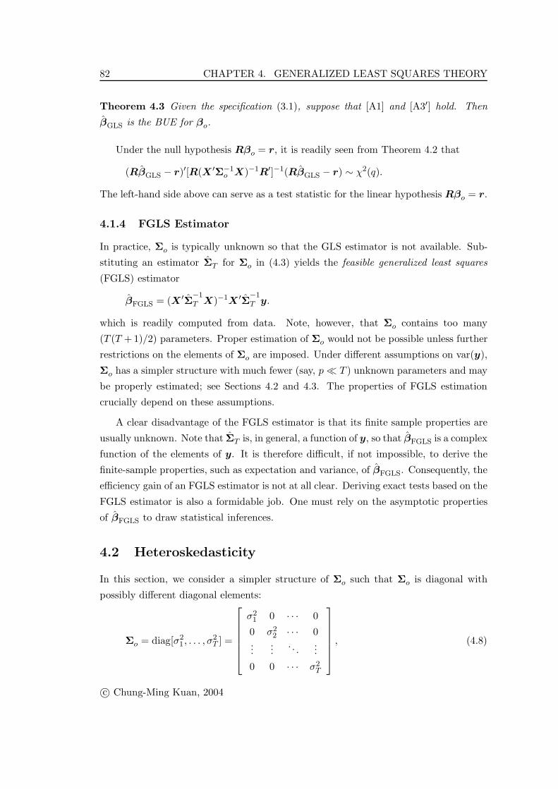
Theorem 4.3 Given the specification (3.1), suppose that [A1] and [A3′] hold. Then

βGLS is the BUE for βo.

Under the null hypothesis Rβo = r, it is readily seen from Theorem 4.2 that

(RβGLS − r)′[R(X ′Σ−1o X)−1R′]−1(RβGLS − r) ∼ χ2(q).

The left-hand side above can serve as a test statistic for the linear hypothesis Rβo = r.

4.1.4 FGLS Estimator

In practice, Σo is typically unknown so that the GLS estimator is not available. Sub-

stituting an estimator ΣT for Σo in (4.3) yields the feasible generalized least squares

(FGLS) estimator

βFGLS = (X ′Σ−1T X)−1X ′Σ

−1T y.

which is readily computed from data. Note, however, that Σo contains too many

(T (T + 1)/2) parameters. Proper estimation of Σo would not be possible unless further

restrictions on the elements of Σo are imposed. Under different assumptions on var(y),

Σo has a simpler structure with much fewer (say, p � T ) unknown parameters and may

be properly estimated; see Sections 4.2 and 4.3. The properties of FGLS estimation

crucially depend on these assumptions.

A clear disadvantage of the FGLS estimator is that its finite sample properties are

usually unknown. Note that ΣT is, in general, a function of y, so that βFGLS is a complex

function of the elements of y. It is therefore difficult, if not impossible, to derive the

finite-sample properties, such as expectation and variance, of βFGLS. Consequently, the

efficiency gain of an FGLS estimator is not at all clear. Deriving exact tests based on the

FGLS estimator is also a formidable job. One must rely on the asymptotic properties

of βFGLS to draw statistical inferences.

4.2 Heteroskedasticity

In this section, we consider a simpler structure of Σo such that Σo is diagonal with

possibly different diagonal elements:

Σo = diag[σ21 , . . . , σ

2T ] =

⎡⎢⎢⎢⎢⎢⎣σ2

1 0 · · · 0

0 σ22 · · · 0

......

. . ....

0 0 · · · σ2T

⎤⎥⎥⎥⎥⎥⎦ , (4.8)


4.2. HETEROSKEDASTICITY 83

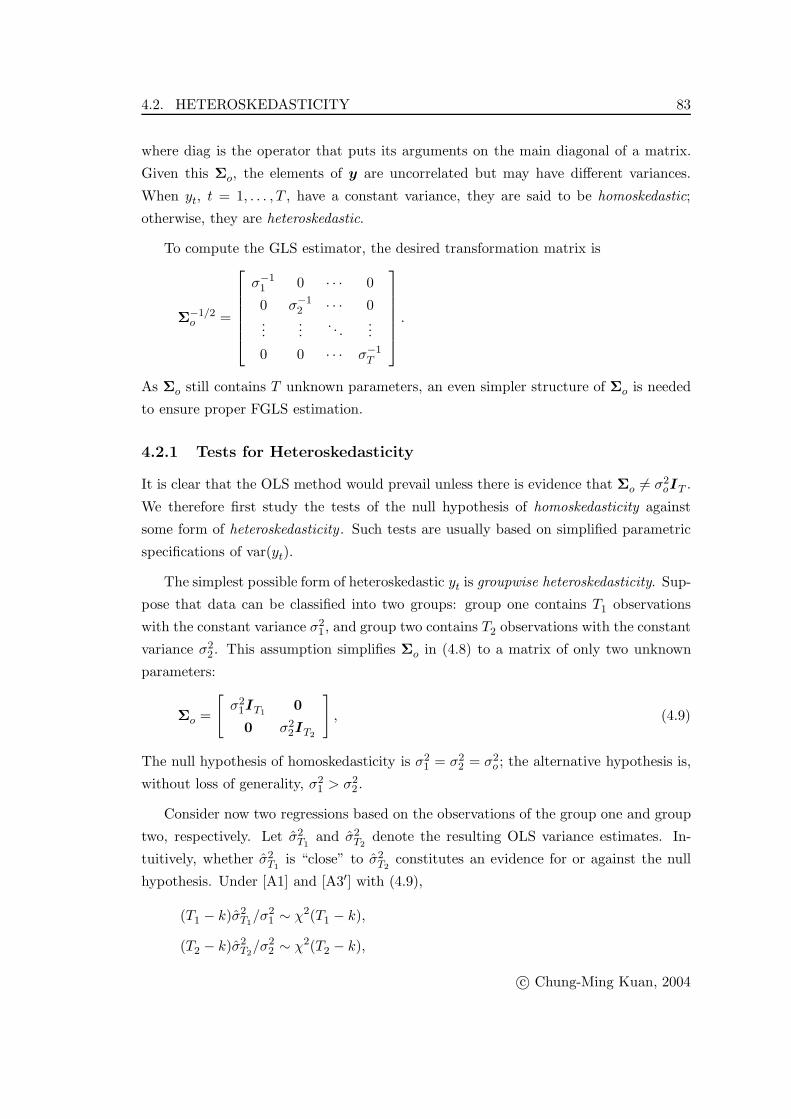
where diag is the operator that puts its arguments on the main diagonal of a matrix.

Given this Σo, the elements of y are uncorrelated but may have different variances.

When yt, t = 1, . . . , T , have a constant variance, they are said to be homoskedastic;

otherwise, they are heteroskedastic.

To compute the GLS estimator, the desired transformation matrix is

Σ−1/2o =

⎡⎢⎢⎢⎢⎢⎣σ−1

1 0 · · · 0

0 σ−12 · · · 0

......

. . ....

0 0 · · · σ−1T

⎤⎥⎥⎥⎥⎥⎦ .

As Σo still contains T unknown parameters, an even simpler structure of Σo is needed

to ensure proper FGLS estimation.

4.2.1 Tests for Heteroskedasticity

It is clear that the OLS method would prevail unless there is evidence that Σo �= σ2oIT .

We therefore first study the tests of the null hypothesis of homoskedasticity against

some form of heteroskedasticity . Such tests are usually based on simplified parametric

specifications of var(yt).

The simplest possible form of heteroskedastic yt is groupwise heteroskedasticity. Sup-

pose that data can be classified into two groups: group one contains T1 observations

with the constant variance σ21 , and group two contains T2 observations with the constant

variance σ22 . This assumption simplifies Σo in (4.8) to a matrix of only two unknown

parameters:

Σo =

[σ2

1IT10

0 σ22IT2

], (4.9)

The null hypothesis of homoskedasticity is σ21 = σ2

2 = σ2o ; the alternative hypothesis is,

without loss of generality, σ21 > σ2

2 .

Consider now two regressions based on the observations of the group one and group

two, respectively. Let σ2T1

and σ2T2

denote the resulting OLS variance estimates. In-

tuitively, whether σ2T1

is “close” to σ2T2

constitutes an evidence for or against the null

hypothesis. Under [A1] and [A3′] with (4.9),

(T1 − k)σ2T1

/σ21 ∼ χ2(T1 − k),

(T2 − k)σ2T2

/σ22 ∼ χ2(T2 − k),



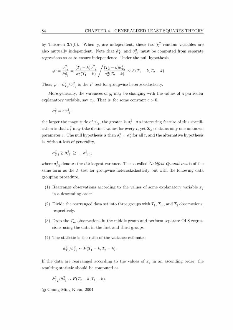
by Theorem 3.7(b). When yt are independent, these two χ2 random variables are

also mutually independent. Note that σ2T1

and σ2T2

must be computed from separate

regressions so as to ensure independence. Under the null hypothesis,

ϕ :=σ2

T1

σ2T2

=(T1 − k)σ2

T1

σ2o(T1 − k)

/(T2 − k)σ2

T2

σ2o(T2 − k)

∼ F (T1 − k, T2 − k).

Thus, ϕ = σ2T1

/σ2T2

is the F test for groupwise heteroskedasticity.

More generally, the variances of yt may be changing with the values of a particular

explanatory variable, say xj . That is, for some constant c > 0,

σ2t = c x2

tj ;

the larger the magnitude of xtj , the greater is σ2t . An interesting feature of this specifi-

cation is that σ2t may take distinct values for every t, yet Σo contains only one unknown

parameter c. The null hypothesis is then σ2t = σ2

o for all t, and the alternative hypothesis

is, without loss of generality,

σ2(1) ≥ σ2

(2) ≥ . . . σ2(T ),

where σ2(i) denotes the i th largest variance. The so-called Goldfeld-Quandt test is of the

same form as the F test for groupwise heteroskedasticity but with the following data

grouping procedure.

(1) Rearrange observations according to the values of some explanatory variable xj

in a descending order.

(2) Divide the rearranged data set into three groups with T1, Tm, and T2 observations,

respectively.

(3) Drop the Tm observations in the middle group and perform separate OLS regres-

sions using the data in the first and third groups.

(4) The statistic is the ratio of the variance estimates:

σ2T1

/σ2T2

∼ F (T1 − k, T2 − k).

If the data are rearranged according to the values of xj in an ascending order, the

resulting statistic should be computed as

σ2T2

/σ2T1

∼ F (T2 − k, T1 − k).


4.2. HETEROSKEDASTICITY 85

In a time-series study, if the variances are conjectured to be decreasing (increasing)

over time, data rearrangement would not be needed. In the procedure for computing

the Goldfeld-Quandt test, dropping observations in the middle group is to enhance the

test’s ability of discriminating variances in the first and third groups. A rule of thumb

suggests that no more than one third of the observations should be dropped; it is also

typical to set T1 ≈ T2. Clearly, this test would be powerful provided that one can

correctly identify the source of heteroskedasticity (i.e., the explanatory variable that

determines variances). On the other hand, finding such a variable may not be an easy

job.

An even more general form of heteroskedastic covariance matrix is such that the

diagonal elements

σ2t = h(α0 + z′

tα1),

where h is some function and zt is a p × 1 vector of exogenous variables affecting the

variances of yt. This assumption simplifies Σo to a matrix of p+1 unknown parameters.

Tests against this class of alternatives can be derived under the likelihood framework,

and their distributions can only be analyzed asymptotically. This will not be discussed

until Chapter 10.

4.2.2 GLS Estimation

If the test for groupwise heteroskedasticity rejects the null hypothesis, one might believe

that Σo is given by (4.9). Accordingly, the specified linear specification may be written

as: [y1

y2

]=

[X1

X2

]β +

[e1

e2

],

where y1 is T1 × 1, y2 is T2 × 1, X1 is T1 × k, and X2 is T2 × k. A transformed

specification is[y1/σ1

y2/σ2

]=

[X1/σ1

X2/σ2

]β +

[e1/σ1

e2/σ2

],

where the transformed yt, t = 1, . . . , T , have constant variance one. It follows that the

GLS and FGLS estimators are, respectively,

βGLS =[X ′

1X1

σ21

+X ′

2X2

σ22

]−1 [X ′

1y1

σ21

+X ′

2y2

σ22

],

βFGLS =[X ′

1X1

σ21

+X ′

2X2

σ22

]−1 [X ′

1y1

σ21

+X ′

2y2

σ22

],



where σ2T1

and σ2T2

are, again, the OLS variance estimates obtained from separate re-

gressions using T1 and T2 observations, respectively. Observe that βFGLS is not a linear

estimator in y so that its finite-sample properties are not known.

If the Goldfeld-Quandt test rejects the null hypothesis, one might believe that σ2t =

c x2tj . A transformed specification is then

yt

xtj

= βj + β1

1xtj

+ · · · + βj−1

xt,j−1

xtj

+ βj+1

xt,j+1

xtj

+ · · · + βk

xtk

xtj

+et

xtj

,

where var(yt/xtj) = c := σ2o . This is a very special case where the GLS estimator is

readily computed as the OLS estimator for the transformed specification. Clearly, the

validity of the GLS method crucially depends on whether the explanatory variable xj

can be correctly identified.

When σ2t = h(α0 + z′

tα1), it is typically difficult to implement an FGLS estimator,

especially when h is nonlinear. If h is the identity function, one may regress the squared

OLS residuals e2t on zt to obtain estimates for α0 and α1. Of course, certain con-

straint must be imposed to ensure the fitted values are non-negative. The finite-sample

properties of this estimator are, again, difficult to analyze.

Remarks:

1. When a test for heteroskedasticity rejects the null hypothesis, there is no guaran-

tee that the alternative hypothesis (say, groupwise heteroskedasticity) must be a

correct description of var(yt).

2. When a form of heteroskedasticity is incorrectly specified, it is also possible that

the resulting FGLS estimator is less efficient than the OLS estimator.

3. As discussed in Section 4.1.3, the finite-sample properties of FGLS estimators and

hence the exact tests are usually not available. One may appeal to asymptotic

theory to construct proper tests.

4.3 Serial Correlation

Another leading example that var(y) �= σ2oIT is when the elements of y are correlated

so that the off-diagonal elements of Σo are non-zero. This phenomenon is more com-

mon in time series data, though it is not necessary so. When time series data yt are

correlated over time, they are said to exhibit serial correlation. For cross-section data,

the correlations of yt are usually referred to as spatial correlation. Our discussion in

this section will concentrate on serial correlation only.


4.3. SERIAL CORRELATION 87

4.3.1 A Simple Model of Serial Correlation

Consider time series yt, t = 1, . . . , T , with the constant variance σ2o . The correlation

coefficient between yt and yt−i is

corr(yt, yt−i) =cov(yt, yt−i)√

var(yt)√

var(yt−i)=

cov(yt, yt−i)σ2

o

,

for i = 0, 1, 2, . . . , t − 1; in particular, corr(yt, yt) = 1. Such correlations are also known

as the autocorrelations of yt. Similarly, cov(yt, yt−i), i = 0, 1, 2, . . . , t − 1, are known as

the autocovariances of yt.

A very simple specification of autocovariances is

cov(yt, yt−i) = cov(yt, yt+i) = ciσ2o ,

where c is a constant such that |c| < 1. Hence, corr(yt, yt−i) = ci. In this specification,

the autocovariances and autocorrelations depend only i, the time periods between two

observations, but not on t. Moreover, the correlations between two observations decay

exponentially fast when i increases. Hence, closer observatins have higher correlations;

two observations would have little correlation if they are separated by a sufficiently long

period. Equivalently, we may write

cov(yt, yt−i) = c cov(yt, yt−i+1).

Letting corr(yt, yt−i) = ρi, we have

ρi = c ρi−1. (4.10)

From this recursion we immediately see that c = ρ1 which must be bounded between

−1 and 1. It follows that var(y) is

Σo = σ2o

⎡⎢⎢⎢⎢⎢⎢⎢⎣

1 ρ1 ρ21 · · · ρT−1

1

ρ1 1 ρ1 · · · ρT−21

ρ21 ρ1 1 · · · ρT−3

1...

......

. . ....

ρT−11 ρT−2

1 ρT−31 · · · 1

⎤⎥⎥⎥⎥⎥⎥⎥⎦. (4.11)

To avoid singularity, ρ1 cannot be ±1.

A novel feature of this specification is that it, while permitting non-zero off-diagonal

elements of Σo, involves only two unknown parameters: σ2o and ρ1. The transformation



matrix is then

Σ−1/2o =

1σo

⎡⎢⎢⎢⎢⎢⎢⎢⎢⎢⎢⎢⎢⎣

1 0 0 · · · 0 0

− ρ1√1−ρ2

1

1√1−ρ2

1

0 · · · 0 0

0 − ρ1√1−ρ2

1

1√1−ρ2

1

· · · 0 0...

......

. . ....

...

0 0 0 · · · 1√1−ρ2

1

0

0 0 0 · · · − ρ1√1−ρ2

1

1√1−ρ2

1

⎤⎥⎥⎥⎥⎥⎥⎥⎥⎥⎥⎥⎥⎦.

Note that this choice of Σ−1/2o is not symmetric. As any matrix that is a constant

proportion to Σ−1/2o can also serve as a transformation matrix for GLS estimation, the

so-called Cochrane-Orcutt Transformation is based on

V −1/2o = σo

√1 − ρ2

1 Σ−1/2o =

⎡⎢⎢⎢⎢⎢⎢⎢⎢⎢⎢⎣

√1 − ρ2

1 0 0 · · · 0 0

−ρ1 1 0 · · · 0 0

0 −ρ1 1 · · · 0 0...

......

. . ....

...

0 0 0 · · · 1 0

0 0 0 · · · −ρ1 1

⎤⎥⎥⎥⎥⎥⎥⎥⎥⎥⎥⎦,

which depends only on ρ1.

The data from the Cochrane-Orcutt transformation are

y∗1 = (1 − ρ21)

1/2y1, x∗1 = (1 − ρ2

1)1/2x1,

y∗t = yt − ρ1yt−1, x∗t = xt − ρ1xt−1, t = 2, · · · , T,

where xt is the t thcolumn of X ′. It is then clear that

var(y∗1) = (1 − ρ21)σ

2o ,

var(y∗t ) = σ2o + ρ2

1σ2o − 2ρ2

1σ2o = (1 − ρ2

1)σ2o , t = 2, . . . , T.

Moreover, for each i,

cov(y∗t , y∗t−i) = cov(yt, yt−i) − ρ1 cov(yt−1, yt−i) − ρ1 cov(yt, yt−i−1)

+ ρ21 cov(yt−1, yt−i−1)

= 0.

Hence, the transformed variable y∗t satisfies the classical conditions, as it ought to be.

Then provided that ρ1 is known, regressing y∗t on x∗t yields the GLS estimator for βo.



4.3.2 An Alternative View

There is an alternative approach to generating the variance-covariance matrix (4.11).

Under [A2](i), let

ε := y − Xβo

denote the deviations of y from its mean vector. This vector is usually referred to as

the vector of disturbances. Note that ε is not the same as the residual vector e. While

the former is not observable because βo is unknown, the later is obtained from OLS

estimation and hence observable. Under [A2], IE(ε) = 0 and

var(y) = var(ε) = IE(εε′).

The variance and covariance structure of y is thus the same as that of ε.

A time series is said to be weakly stationary if its mean, variance, and autocovari-

ances are all independent of the time index t. Thus, a weakly stationary series can not

exhibit trending behavior, nor can it generate very large fluctuatinos. In particular,

a time series with zero mean, a constant variance, and zero autocovariances is weakly

stationary; such a process is also known as a white noise. Let {ut} be a white noise with

IE(ut) = 0, IE(u2t ) = σ2

u, and IE(utuτ ) = 0 for t �= τ . Now suppose that the elements of

ε is generated as a weakly stationary AR(1) process (autoregressive process of order 1):

εt = α1εt−1 + ut, (4.12)

with ε0 = 0. By recursive substitution, (4.12) can be expressed as

εt =t−1∑i=0

αi1ut−i, (4.13)

a weighted sum of current and previous random innovations (shocks).

It follows from (4.13) that IE(εt) = 0 and IE(ut, εt−s) = 0 for all t and s ≥ 1. By

weak stationarity, var(εt) is a constant, so that for all t,

var(εt) = α21 var(εt−1) + σ2

u = σ2u/(1 − α2

1).

Clearly, the right-hand side would not be meaningful unless |α1| < 1. The autocovari-

ance of εt and εt−1 is, by weak stationarity,

IE(εtεt−1) = α1 IE(ε2t−1) = α1

σ2u

1 − α21

.



This shows that

α1 = corr(εt, εt−1) = corr(yt, yt−1) = ρ1.

Similarly,

IE(εtεt−2) = α1 IE(εt−1εt−2) = α21

σ2u

1 − α21

,

so that

corr(εt, εt−2) = α1 corr(εt, εt−1) = ρ21.

More generally, we can write for i = 1, 2, . . .,

corr(εt, εt−i) = ρ1 corr(εt, εt−i+1) = ρi1,

which depend only on i, the time difference between two ε’s, but not on t. This is

precisely what we postulated in (4.10). The variance-covariance matrix Σo under this

structure is also (4.11) with σ2o = σ2

u/(1 − ρ21).

The AR(1) structure of disturbances also permits a straightforward extension. Con-

sider the disturbances that are generated as an AR(p) process (autoregressive process

of order p):

εt = α1εt−1 + · · · + αpεt−p + ut, (4.14)

where the coefficients α1, . . . , αp should also be restricted to ensure weak stationarity;

we omit the details. Of course, εt may follow different structures and are still serially

correlated. For example, εt may be generated as an MA(1) process (moving average

process of order 1):

εt = ut + α1ut−1, |α1| < 1,

where {ut} is a white noise; see e.g., Exercise 4.6.

4.3.3 Tests for AR(1) Disturbances

As the AR(1) structure of disturbances is one of the most commonly used specification of

serial correlation, we now consider the tests of the null hypothesis of no serial correlation

(α1 = ρ1 = 0) against AR(1) disturbances. We discuss only the celebrated Durbin-

Watson test and Durbin’s h test; the discussion of other large-sample tests will be

deferred to Chapter 6.



In view of the AR(1) structure, a natural estimator of ρ1 is the OLS estimator of

regressing the OLS residual et on its immediate lag et−1:

ρT =∑T

t=2 etet−1∑Tt=2 e2

t−1

. (4.15)

The Durbin-Watson statistic is

d =∑T

t=2(et − et−1)2∑T

t=1 e2t

.

When the sample size T is large, it can be seen that

d = 2 − 2ρT

∑Tt=2 e2

t−1∑Tt=1 e2

t

− e21 + e2

T∑Tt=1 e2

t

≈ 2(1 − ρT ).

For 0 < ρT ≤ 1 (−1 ≤ ρT < 0), the Durbin-Watson statistic is such that 0 ≤ d < 2

(2 < d ≤ 4), which suggests that there is some positive (negative) serial correlation.

Hence, this test essentially checks whether ρT is sufficiently “close” to zero (i.e., d is

close to 2).

A major difficulty of the Durbin-Watson test is that the exact null distribution of d

depends on the matrix X and therefore varies with data. (Recall that the t and F tests

discussed in Section 3.3.1 have, respectively, t and F distributions regardless of the data

X .) This drawback prevents us from tabulating the critical values of d. Nevertheless, it

has been shown that the null distribution of d lies between the distributions of a lower

bound (dL) and an upper bound (dU ) in the sense that for any significance level α,

d∗L,α < d∗α < d∗U,α,

where let d∗α, d∗L,α and d∗U,α denote, respectively, the critical values of d, dL and dU .

Although the distribution of d is data dependent, the distributions of dL and dU are

not. Thus, the critical values d∗L,α and d∗U,α can be tabulated. One may then rely on

these critical values to construct a “conservative” decision rule.

Specifically, when the alternative hypothesis is ρ1 > 0 (ρ1 < 0), the decision rule of

the Durbin-Watson test is:

(1) Reject the null if d < d∗L,α (d > 4 − d∗L,α).

(2) Do not reject the null if d > d∗U,α (d < 4 − d∗U,α).



(3) Test is inconclusive if d∗L,α < d < d∗U,α (4 − d∗L,α > d > 4 − d∗U,α).

This is not completely satisfactory because the test may yield no conclusion. Some

econometric packages such as SHAZAM now compute the exact Durbin-Watson dis-

tribution for each regression and report the exact p-values. When such a program is

available, this test does not have to rely on the critical values of dL and dU and hence

must be conclusive. Note that the tabulated critical values of the Durbin-Watson statis-

tic are for the specifications with a constant term; the critical values for the specifications

without a constant term can be found in Farebrother (1980).

Another problem with the Durbin-Watson statistic is that its null distribution holds

only under the classical conditions [A1] and [A3]. In the time series context, it is quite

common to include a lagged dependent variable as a regressor so that [A1] is violated.

A leading example is the specification

yt = β1 + β2xt2 + · · · + βkxtk + γyt−1 + et.

This model can also be derived from certain behavioral assumptions; see Exercise 4.7.

It has been shown that the Durbin-Watson statistic under this specification is biased

toward 2. That is, this test would not reject the null hypothesis even when serial

correlation is present. On the other hand, Durbin’s h test is designed specifically for

the specifications that contain a lagged dependent variable. Let γT be the OLS estimate

of γ and var(γT ) be the OLS estimate of var(γT ). The h statistic is

h = ρT

√T

1 − T var(γT ),

and its asymptotic null distribution is N (0, 1). A clear disadvantage of Durbin’s h test

is that it can not be calculated when var(γT ) ≥ 1/T . This test can also be derived as a

Lagrange Multiplier test under the likelihood framework; see Chapter 10

If we have quarterly data and want to test for the fourth-order serial correlation,

the statistic analogous to the Durbin-Watson statistic is

d4 =∑T

t=5(et − et−4)2∑Tt=1 e2

t

;

see Wallis (1972) for corresponding critical values.

4.3.4 FGLS Estimation

Recall that Σo depends on two parameters σ2o and ρ1. We may use a generic notation

Σ(σ2, ρ) to denote this function of σ2 and ρ. In particular, Σo = Σ(σ2o , ρ1). Similarly, we



may also write V (ρ) such that V o = V (ρ1). The transformed data based on V (ρ)−1/2

are

y1(ρ) = (1 − ρ2)1/2y1, x1(ρ) = (1 − ρ2)1/2x1,

yt(ρ) = yt − ρyt−1, xt(ρ) = xt − ρxt−1, t = 2, · · · , T.

Hence, y∗t = yt(ρ1) and x∗t = xt(ρ1).

To obtain an FGLS estimator, we must first estimate ρ1 by some estimator ρT and

then construct the transformation matrix as V−1/2T = V (ρT )−1/2. Here, ρT may be com-

puted as in (4.15); other estimators for ρ1 may also be used, e.g., ρT = ρT (T−k)/(T−1).

The transformed data are then yt(ρT ) and xt(ρT ). An FGLS estimator is obtained by

regressing yt(ρT ) on xt(ρT ). Such an estimator is known as the Prais-Winsten estimator

or the Cochrane-Orcutt estimator when the first observation is dropped in computation.

The following iterative procedure is also commonly employed in practice.

(1) Perform OLS estimation and compute ρT as in (4.15) using the OLS residuals et.

(2) Perform the Cochrane-Orcutt transformation based on ρT and compute the re-

sulting FGLS estimate βFGLS by regressing yt(ρT ) on xt(ρT ).

(3) Compute a new ρT as in (4.15) with et replaced by the FGLS residuals

et,FGLS = yt − x′tβFGLS.

(4) Repeat steps (2) and (3) until ρT converges numerically, i.e., when ρT from two

consecutive iterations differ by a value smaller than a pre-determined convergence

criterion.

Note that steps (1) and (2) above already generate an FGLS estimator. More iterations

do not improve the asymptotic properties of the resulting estimator but may have a

significant effect in finite samples. This procedure can be extended easily to estimate

the specification with higher-order AR disturbances.

Alternatively, the Hildreth-Lu procedure adopts grid search to find the ρ1 ∈ (−1, 1)

that minimizes the sum of squared errors of the model. This procedure is computation-

ally intensive, and it is difficult to implement when εt have an AR(p) structure with

p > 2.

In view of the log-likelihood function (4.7), we must compute det(Σo). Clearly,

det(Σo) =1

det(Σ−1o )

=1

[det(Σ−1/2o )]2

.



In terms of the notations in the AR(1) formulation, σ2o = σ2

u/(1 − ρ21), and

Σ−1/2o =

1σo

√1 − ρ2

1

V −1/2o =

1σu

V −1/2o .

As det(V −1/2o ) = (1 − ρ2

1)1/2, we then have

det(Σo) = (σ2u)T (1 − ρ2

1)−1.

The log-likelihood function for given σ2u and ρ1 is

log L(β;σ2u, ρ1)

= −T

2log(2π) − T

2log(σ2

u) +12

log(1 − ρ21) −

12σ2

u

(y∗ − X∗β)′(y∗ − X∗β).

Clearly, when σ2u and ρ1 are known, the MLE of β is just the GLS estimator.

If σ2u and ρ1 are unknown, the log-likelihood function reads:

log L(β, σ2, ρ)

= −T

2log(2π) − T

2log(σ2) +

12

log(1 − ρ2) − 12σ2

(1 − ρ2)(y1 − x′1β)2

− 12σ2

T∑t=2

[(yt − x′tβ) − ρ(yt−1 − x′

t−1β)]2,

which is a nonlinear function of the parameters. Nonlinear optimization methods (see,

e.g., Section 8.2.2) are therefore needed to compute the MLEs of β, σ2, and ρ. For

a given β, estimating ρ by regressing et(β) = yt − x′tβ on et−1(β) is equivalent to

maximizing the last term of the log-likelihood function above. This does not yield an

MLE because the other terms involving ρ, namely,

12

log(1 − ρ2) − 12σ2

(1 − ρ2)(y1 − x′1β)2,

have been ignored. This shows that the aforementioned iterative procedure does not

result in the MLEs.

Remark: Exact tests based on FGLS estimation results are not available because the

finite-sample distribution of the FGLS estimator is, again, unknown. Asymptotic theory

is needed to construct proper tests.


4.4. APPLICATION: LINEAR PROBABILITY MODEL 95

4.4 Application: Linear Probability Model

In some applications researchers are interested in analyzing why consumers own a house

or participate a particular event. The ownership or the choice of participation are

typically represented by a binary variable that takes the values one and zero. If the

dependent variable in a linear regression is binary, we will see below that both the OLS

and FGLS methods are not appropriate.

Let xt denote the t th column of X ′. The t th observation of the linear specification

y = Xβ + e can be expressed as

yt = x′tβ + et.

For the binary dependent variable y whose t th observation is yt = 1 or 0, we know

IE(yt) = IP(yt = 1).

Thus, x′tβ is just a specification of the probability that yt = 1. As such, the linear

specification of binary dependent variables is usually referred to as the linear probability

model.

When [A1] and [A2](i) hold for a linear probability model,

IE(yt) = IP(yt = 1) = x′tβo,

and the OLS estimator is unbiased for βo. Note, however, that the variance of yt is

var(yt) = IP(yt = 1)[1 − IP(yt = 1)].

Under [A1] and [A2](i),

var(yt) = x′tβo(1 − x′

tβo),

which varies with xt. Thus, the linear probability model suffers from the problem of

heteroskedasticity, and the OLS estimator is not the BLUE for βo. Apart from the

efficiency issue, the OLS method is still not appropriate for the linear probability model

because the OLS fitted values need not be bounded between zero and one. When x′tβT

is negative or greater than one, it can not be interpreted as a probability.

Although the GLS estimator is the BLUE, it is not available because βo, and hence

var(yt), is unknown. Nevertheless, if yt are uncorrelated so that var(y) is diagonal, an

FGLS estimator may be obtained using the transformation matrix

Σ−1/2T = diag

[x′

1βT (1 − x′1βT )]−1/2,x′

2βT (1 − x′2βT )]−1/2, . . . ,

x′T βT (1 − x′

T βT )]−1/2],



where βT is the OLS estimator of βo. Such an estimator breaks down when Σ−1/2T

cannot be computed (i.e., when x′tβT is negative or greater than one). Even when

Σ−1/2T is available, there is still no guarantee that the FGLS fitted values are bounded

between zero and one. This shows that the FGLS method may not always be a solution

when the OLS method fails.

This example also illustrates the importance of data characteristics in estimation and

modeling. Without taking into account the binary nature of the dependent variable,

even the FGLS method may be invalid. More appropriate methods for specifications

with binary dependent variables will be discussed in Chapter 10.

4.5 Seemingly Unrelated Regressions

In many econometric practices, it is important to study the joint behavior of several

dependent variables. For example, the input demands of an firm may be described using

a system of linear regression functions in which each regression represents the demand

function of a particular input. It is intuitively clear that these input demands ought to

be analyzed jointly because they are related to each other.

Consider the specification of a system of N equations, each with ki explanatory

variables and T observations. Specifically,

yi = Xiβi + ei, i = 1, 2, . . . , N, (4.16)

where for each i, yi is T × 1, Xi is T × ki, and βi is ki × 1. The system (4.16) is

also known as a specification of seemingly unrelated regressions (SUR). Stacking the

equations of (4.16) yields⎡⎢⎢⎢⎢⎢⎣y1

y2...

yN

⎤⎥⎥⎥⎥⎥⎦︸︷︷︸

y

=

⎡⎢⎢⎢⎢⎢⎣X1 0 · · · 0

0 X2 · · · 0...

.... . .

...

0 0 · · · XN

⎤⎥⎥⎥⎥⎥⎦︸︷︷︸

X

⎡⎢⎢⎢⎢⎢⎣β1

β2...

βN

⎤⎥⎥⎥⎥⎥⎦︸︷︷︸

β

+

⎡⎢⎢⎢⎢⎢⎣e1

e2...

eN

⎤⎥⎥⎥⎥⎥⎦︸︷︷︸

e

. (4.17)

This is a linear specification (3.1) with k =∑N

i=1 ki explanatory variables and TN obser-

vations. It is not too hard to see that the whole system (4.17) satisfies the identification

requirement whenever every specification of (4.16) does.

Suppose that the classical conditions [A1] and [A2] hold for each specified linear

regression in the system. Then under [A2](i), there exists βo = (β′o,1 . . . β′

o,N )′ such


4.5. SEEMINGLY UNRELATED REGRESSIONS 97

that IE(y) = Xβo. The OLS estimator obtained from (4.17) is therefore unbiased.

Note, however, that [A2](ii) for each linear regression ensures that, for each i,

var(yi) = σ2i IT ;

there is no restriction on the correlations between yi and yj. The variance-covariance

matrix of y is then

var(y) = Σo =

⎡⎢⎢⎢⎢⎢⎣σ2

1IT cov(y1,y2) · · · cov(y1,yN )

cov(y2,y1) σ22IT · · · cov(y2,yN )

......

. . ....

cov(yN ,y1) cov(yN ,y2) · · · σ2NIT

⎤⎥⎥⎥⎥⎥⎦ . (4.18)

This shows that y, the vector of stacked dependent variables, violates [A2](ii), even

when each individual dependent variable has a scalar variance-covariance matrix. Con-

sequently, the OLS estimator of the whole system, βTN = (X ′X)−1X ′y, is not the

BLUE in general. In fact, owing to the block-diagonal structure of X, βTN simply

consists of N equation-by-equation OLS estimators and hence ignores the correlations

between equations and heteroskedasticity across equations.

In practice, it is also typical to postulate that for i �= j,

cov(yi,yj) = σijIT ,

that is, yit and yjt are contemporaneously correlated but yit and yjτ , t �= τ , are serially

uncorrelated. Under this condition, (4.18) simplifies to Σo = So ⊗ IT with

So =

⎡⎢⎢⎢⎢⎢⎣σ2

1 σ12 · · · σ1N

σ21 σ22 · · · σ2N

......

. . ....

σN1 σN2 · · · σ2N

⎤⎥⎥⎥⎥⎥⎦ . (4.19)

As Σ−1o = S−1

o ⊗ IT , the GLS estimator of (4.17) is

βGLS = [X ′(S−1o ⊗ IT )X]−1X ′(S−1

o ⊗ IT )y,

and its covariance matrix is [X ′(S−1o ⊗ IT )X]−1.

It is readily verified that when σij = 0 for all i �= j, So becomes a diagonal matrix,

and so is Σo. Then, the resulting GLS estimator reduces to the OLS estimator. This

should not be too surprising because estimating a SUR system would be unnecessary



if the dependent variables are in fact uncorrelated. (Note that the heteroskedasticity

across equations does not affect this result.) If all equations in the system have the

same regressors, i.e., Xi = X0 (say), the GLS estimator is also the same as the OLS

estimator; see e.g., Exercise 4.8. More generally, it can be shown that there would not

be much efficiency gain for GLS estimation if yi and yj are less correlated and/or Xi

and Xj are highly correlated; see e.g., Goldberger (1991, p. 328) for an illustrative

example.

The FGLS estimator is now readily obtained by replacing S−1o with S

−1TN , where

STN is an N × N matrix computed as

STN =1T

⎡⎢⎢⎢⎢⎢⎣e′

1

e′2...

e′N

⎤⎥⎥⎥⎥⎥⎦[

e1 e2 . . . eN

],

where ei is the OLS residual vector of the i th equation. The elements of this matrix

are

σ2i =

e′iei

T, i = 1, . . . , N,

σij =e′

iej

T, i �= j, i, j = 1, . . . , N.

Note that STN is of an outer product form and hence a positive semi-definite matrix.

One may also replace the denominator of σ2i with T − ki and the denominator of σij

with T − max(ki, kj). The resulting estimator STN need not be positive semi-definite,

however.

Remark: The estimator STN mentioned above is valid provided that var(yi) = σ2i IT

and cov(yi,yj) = σijIT . If these assumptions do not hold, FGLS estimation would be

much more complicated. This may happen when heteroskedasticity and serial correla-

tions are present in each equation, or when cov(yit, yjt) changes over time.

4.6 Models for Panel Data

A data set that contains a collection of cross-section units (individuals, families, firms, or

countries), each with some time-series observations, is known as a panel data set. Well

known panel data sets in the U.S. include the National Longitudinal Survey of Labor

Market Experience and the Michigan Panel Study of Income Dynamics. Building such


4.6. MODELS FOR PANEL DATA 99

data sets is very costly because they are obtained by tracking thousands of individuals

through time. Some panel data may be easier to establish; for example, the GDP data

for all G7 countries over 50 years also form a panel data set.

Panel data contain richer information than pure cross-section or time-series data.

On one hand, panel data offer a description of the dynamics of each cross-section unit.

On the other hand, panel data are able to reveal the variations of dynamic patterns

across individual units. Thus, panel data may render more precise parameter estimates

and permit analysis of topics that could not be studied using only cross-section or time-

series data. For example, to study whether each individual unit i has its own pattern, a

specification with parameter(s) changing with i is needed. Such specifications can not

be properly estimated using only cross-section data because the number of parameters

must exceed the number of observations. The problem may be circumvented by using

panel data. In what follows we will consider specifications for panel data that allow

parameter to change across individual units.

4.6.1 Fixed-Effects Model

Given a panel data set with N cross-section units and T observations, the linear speci-

fication allowing for individual effects is

yit = x′itβi + eit, i = 1, . . . , N, t = 1, . . . , T,

where xit is k × 1 and βi is the parameter vector depending only on i but not on t.

In this specification, individual effects are characterized by βi, and there is no time-

specific effect. This may be reasonable when a short time series is observed for each

individual unit. Analogous to the notations in the SUR system (4.16), we can express

the specification above as

yi = Xiβi + ei, i = 1, 2, . . . , N, (4.20)

where yi is T × 1, Xi is T × k, and ei is T × 1. This is a system of equations with

k ×N parameters. Here, the dependent variable y and explanatory variables X are the

same across individual units such that yi and Xi are simply their observations for each

individual i. For example, y may be the family consumption expenditure, and each yi

contains family i’s annual consumption expenditures. By contrast, yi and Xi may be

different variables in a SUR system.

When T is small (i.e., observed time series are short), estimating (4.20) is not feasible.

A simpler form of (4.20) is such that only the intercept changes with i and the other



parameters remain constant across i:

yi = �T ai + Zib + ei, i = 1, 2, . . . , N, (4.21)

where �T is the T -dimensional vector of ones, [�T Zi] = X i and [ai b′]′ = βi. In

(4.21), individual effects are completely captured by the intercept ai. This specification

simplifies (4.20) from kN to N + k − 1 parameters and is known as the fixed-effects

model. Stacking N equations in (4.21) together we obtain⎡⎢⎢⎢⎢⎢⎣y1

y2...

yN

⎤⎥⎥⎥⎥⎥⎦︸︷︷︸

y

=

⎡⎢⎢⎢⎢⎢⎣�T 0 · · · 0

0 �T · · · 0...

.... . .

...

0 0 · · · �T

⎤⎥⎥⎥⎥⎥⎦︸︷︷︸

D

⎡⎢⎢⎢⎢⎢⎣a1

a2...

aN

⎤⎥⎥⎥⎥⎥⎦︸︷︷︸

a

+

⎡⎢⎢⎢⎢⎢⎣Z1

Z2...

ZN

⎤⎥⎥⎥⎥⎥⎦︸︷︷︸

Z

b +

⎡⎢⎢⎢⎢⎢⎣e1

e2...

eN

⎤⎥⎥⎥⎥⎥⎦︸︷︷︸

e

. (4.22)

Clearly, this is still a linear specification with N + k − 1 explanatory variables and TN

observations. Note that each column of D is in effect a dummy variable for the i th

individual unit. In what follows, an individual unit will be referred to as a “group.”

The following notations will be used in the sequel. Let Z ′i ((k − 1) × T ) be the i th

block of Z′ and zit be its t th column. For zit, the i th group average over time is

zi =1T

T∑t=1

zit =1T

Z′i�T ;

the i th group average of yit over time is

yi =1T

T∑t=1

yit =1T

y′i�T .

The overall sample average of zit (average over time and group) is

z =1

TN

N∑i=1

T∑t=1

zit =1

TNZ′�TN ,

and the overall sample average of yit is

y =1

TN

N∑i=1

T∑t=1

yit =1

TNy′�TN .

Observe that the overall sample averages are

z =1N

N∑i=1

zi, y =1N

N∑i=1

yi,



which are the sample averages of group averages.

From (4.22) we can see that this specification satisfies the identification requirement

[ID-1] provided that there is no time invariant regressor (i.e., no column of Z is a

constant). Once this requirement is satisfied, the OLS estimator is readily computed.

By Theorem 3.3, the OLS estimator for b is

bTN = [Z ′(ITN − P D)Z]−1Z ′(ITN − P D)y, (4.23)

where P D = D(D′D)−1D′ is a projection matrix. Thus, bTN can be obtained by

regressing (ITN − P D)y on (ITN − P D)Z. Let aTN denote the OLS estimator of the

vector a of individual effects. By the facts that

D′y = D′DaTN + D′ZbTN ,

and that the OLS residual vector is orthogonal to D, aTN can be computed as

aTN = (D′D)−1D′(y − ZbTN ). (4.24)

We will present alternative expressions for these estimators which yield more intuitive

interpretations.

Writing D = IN ⊗ �T , we have

P D = (IN ⊗ �T )(IN ⊗ �′T �T )−1(IN ⊗ �′T )

= (IN ⊗ �T )[IN ⊗ (�′T �T )−1](IN ⊗ �′T )

= IN ⊗ [�T (�′T �T )−1�′T ]

= IN ⊗ �T �′T /T,

where �T �′T /T is also a projection matrix. Thus,

ITN − P D = IN ⊗ (IT − �T �′T /T ),

and (IT − �T �′T /T )yi = yi − �T yi with the t th element being yit − yi. It follows that

(ITN − P D)y =

⎛⎜⎜⎜⎜⎜⎝y1

y2...

yN

⎞⎟⎟⎟⎟⎟⎠−

⎛⎜⎜⎜⎜⎜⎝�T y1

�T y2...

�T yN

⎞⎟⎟⎟⎟⎟⎠ ,



which is the vector of all the deviations of yit from the group averages yi. Similarly,

(ITN − P D)Z =

⎛⎜⎜⎜⎜⎜⎝Z1

Z2...

ZN

⎞⎟⎟⎟⎟⎟⎠−

⎛⎜⎜⎜⎜⎜⎝�T z′

1

�T z′2

...

�T z′N

⎞⎟⎟⎟⎟⎟⎠ ,

with the t th observation in the i th block being (zit − zi)′, the deviation of zit from

the group average zi. This shows that the OLS estimator (4.23) can be obtained by

regressing yit − yi on zit − zi for i = 1, . . . , N , and t = 1, . . . , T . That is,

bTN =

(N∑

i=1

(Z ′i − zi�

′T )(Zi − �T z′

i)

)−1( N∑i=1

(Z ′i − zi�

′T )(yi − �T yi)

)

=

(N∑

i=1

T∑t=1

(zit − zi)(zit − zi)′)−1( N∑

i=1

T∑t=1

(zit − zi)(yit − yi)

).

(4.25)

The estimator bTN will be referred to as the within-groups estimator because it is based

on the observations that are deviations from their own group averages, as shown in

(4.25). It is also easily seen that the i th element of aTN is

aTN,i =1T

(�′T yi − �′T ZibTN ) = yi − z′ibTN ,

which involves only group averages and the within-groups estimator. To distinguish

aTN and bTN from other estimators, we will suppress their subscript TN and denote

them as aw and bw.

Suppose that the classical conditions [A1] and [A2](i) hold for every equation i in

(4.21) so that

IE(yi) = �T ai,o + Zibo. i = 1, 2, . . . , N.

Then, [A1] and [A2](i) also hold for the entire system (4.22) as

IE(y) = Dao + Zbo,

where the i th element of ao is ai,o. Theorem 3.4(a) now ensures that aw and bw are

unbiased for ao and bo, respectively.

Suppose also that var(yi) = σ2oIT for every equation i and that cov(yi,yj) = 0 for

every i �= j. Under these assumptions, var(y) is the scalar variance-covariance matrix



σ2oITN . By the Gauss-Markov theorem, aw and bw are the BLUEs for ao and bo,

respectively. The variance-covariance matrix of the within-groups estimator is

var(bw) = σ2o [Z

′(ITN − P D)Z]−1

= σ2o

[N∑

i=1

T∑t=1

(zit − zi)(zit − zi)′]−1

.

It is also easy to verify that the variance of the i th element of aw is

var(aw,i) =1T

σ2o + z′

i[var(bw)]zi; (4.26)

see Exercise 4.9. The OLS estimator for the regression variance σ2o in this case is

σ2w =

1TN − N − k + 1

N∑i=1

T∑t=1

(yit − aw,i − z′itbw)2,

which can be used to compute the estimators of var(aw,i) and var(bw).

It should be emphasized that the conditions var(yi) = σ2oIT for all i and cov(yi,yj) =

0 for every i �= j may be much too strong in applications. When any one of these con-

ditions fails, var(y) can not be written as σ2oITN , and aw and bw are no longer the

BLUEs. Despite that var(y) may not be a scalar variance-covariance matrix in prac-

tice, the fixed-effects model is typically estimated by the OLS method and hence also

known as the least squares dummy variable model. For GLS and FGLS estimation see

Exercise 4.10.

If [A3] holds for (4.22) such that

y ∼ N (Dao + Zbo, σ2oITN

),

the t and F tests discussed in Section 3.3 remain applicable. An interesting hypoth-

esis for the fixed-effects model is whether fixed (individual) effects indeed exist. This

amounts to applying an F test to the hypothesis

H0 : a1,o = a2,o = · · · = aN,o.

The null distribution of this F test is F (N − 1, TN − N − k + 1). In practice, it may

be more convenient to estimate the following specification for the fixed-effects model:⎡⎢⎢⎢⎢⎢⎣y1

y2...

yN

⎤⎥⎥⎥⎥⎥⎦ =

⎡⎢⎢⎢⎢⎢⎣�T 0 · · · 0

�T �T · · · 0...

.... . .

...

�T 0 · · · �T

⎤⎥⎥⎥⎥⎥⎦

⎡⎢⎢⎢⎢⎢⎣a1

a2...

aN

⎤⎥⎥⎥⎥⎥⎦+

⎡⎢⎢⎢⎢⎢⎣Z1

Z2...

ZN

⎤⎥⎥⎥⎥⎥⎦ b +

⎡⎢⎢⎢⎢⎢⎣e1

e2...

eN

⎤⎥⎥⎥⎥⎥⎦ . (4.27)



This specification is virtually the same as (4.22), yet the parameters ai, i = 2, . . . , N ,

now denote the differences between the i th and first group effects. Testing the existence

of fixed effects is then equivalent to testing

H0 : a2,o = · · · = aN,o = 0.

This can be easily done using an F test; see Exercise 4.11.

4.6.2 Random-Effects Model

Given the specification (4.21) that allows for individual effects:

yi = �T ai + Zib + ei, i = 1, 2, . . . , N,

we now treat ai as random variables rather than parameters. Writing ai = a + ui with

a = IE(ai), the specification above can be expressed as

yi = �T a + Zib + (�T ui + ei), i = 1, 2, . . . , N. (4.28)

where �T ui and ei form the error term. This specification differs from the fixed-effects

model in that the intercept does not vary across i. The presence of ui also makes (4.28)

different from the specification that does not allow for individual effects. Here, the

group heterogeneity due to individual effects is characterized by the random variables

ui and absorbed into the error term. Thus, (4.28) is known as the random-effects model.

If we apply the OLS method to (4.28), the OLS estimator of b and a are, respectively,

bp =

(N∑

i=1

T∑t=1

(zit − z)(zit − z)′)−1( N∑

i=1

T∑t=1

(zit − z)(yit − y)

), (4.29)

and ap = y − z′bp. Comparing with the within-groups estimator (4.25), bp is based on

the deviations of yit and zit from their respective overall averages y and z, whereas bw

is based on the deviations from group averages yi and zi. Note that we have suppressed

the subscript TN for these two estimators. Alternatively, pre-multiplying �′/T through

equation (4.28) yields

yi = a + z′ib + (ui + ei), i = 1, 2, . . . , N, (4.30)

where ei =∑T

t=1 eit/T . By noting that the sample averages of yi and zi are just y and

z, the OLS estimators for the specification (4.30) are

bb =

(N∑

i=1

(zi − z)(zi − z)′)−1( N∑

i=1

(zi − z)(yi − y)

), (4.31)



and ab = y − z′bb. The estimator bb is known as the between-groups estimator because

it is based on the deviations of group averages from the overall averages. Here, we

suppress the subscript N for ab and bb. It can also be shown that the estimator (4.29) is

a weighted sum of the within-groups estimator (4.25) and the between-group estimator

(4.31); see Exercise 4.12. Thus, bp is known as the pooled estimator.

Suppose that the classical conditions [A1] and [A2](i) hold for every equation i such

that

IE(yi) = �T ao + Zibo, i = 1, . . . , N.

Then, [A1] and [A2](i) hold for the entire system of (4.28) as

IE(y) = �TNao + Zbo.

Moreover, they also hold for the specification (4.30) as

IE(yi) = ao + z′ibo, i = 1, . . . , N.

It follows that ab and bb, as well as ap and bp, are unbiased for ao and bo in the random-

effects model. Moreover, write

yi = �T ao + Zibo + ε∗i , (4.32)

where ε∗i is the sum of two components: the random effects �T ui and the disturbance

εi for equation i. Then,

var(yi) = σ2u�T �′T + var(εi) + 2 cov(�T ui, εi),

where σ2u is var(ui). As the first term on the right-hand side above is a full matrix,

var(yi) is not a scalar variance-covariance matrix in general. Consequently, ap and bp

are not the BLUEs. For the specification (4.30), ab and bb are not the BLUEs unless

more stringent conditions are imposed.

Remark: If the fixed-effects model (4.21) is correct, the random-effects model (4.28)

can be viewed as a specification that omits n−1 relevant dummy variables. This implies

the pooled estimator bp and the between-groups estimator bb are biased for bo in the

fixed-effects model. This should not be too surprising because, while there are N +k−1

parameters in the fixed-effects model, the specification (4.30) only permits estimation

of k parameters. We therefore conclude that neither the between-groups estimator nor

the pooled estimator is a proper choice for the fixed-effects model.



To perform FGLS estimation for the random-effects model, more conditions on

var(yi) are needed. If var(εi) = σ2oIT and IE(uiεi) = 0, var(yi) has a simpler form:

So := var(yi) = σ2u�T �′T + σ2

oIT .

Under the following additional conditions: IE(uiuj) = 0, E(uiεj) = 0 and IE(εiεj) = 0

for all i �= j, we have cov(yi,yj) = 0. Hence, var(y) simplifies to a block diagonal

matrix:

Σo := var(y) = IN ⊗ So,

which is not a scalar variance-covariance matrix unless σ2u = 0. It can be verified that

the desired transformation matrix for GLS estimation is Σ−1/2o = IN ⊗ S

−1/2o , where

S−1/2o = IT − c

T�T �′T ,

and c = 1 − σ2o/(Tσ2

u + σ2o)

1/2. The transformed data are then S−1/2o yi and S

−1/2o Zi,

i = 1, . . . , N , and their t th elements are, respectively, yit− cyi and zit− czi. Regressing

yit − cyi on zit − czi gives the desired GLS estimator.

It can be shown that the GLS estimator is also a weighted average of the within-

groups and between-groups estimators. For the special case that σ2o = 0, we have c = 1

and

Σ−1/2o = IN ⊗ (IT − �T �′T /T ) = ITN − P D,

as in the fixed-effects model. In this case, the GLS estimator of b is nothing but the

within-groups estimator bw. When c = 0, the GLS estimator of b reduces to the pooled

estimator bp.

To compute the FGLS estimator, we must estimate the parameters σ2u and σ2

o in So.

We first eliminate the random effects ui by taking the difference of yi and �T yi:

yi − �T yi = (Zi − �T z′i)bo + (εi − �T εi).

For this specification, the OLS estimator of bo is just the within-groups estimator bw.

As ui have been eliminated, we can estimate σ2o , the variance of εit, by

σ2ε =

1TN − N − k + 1

N∑i=1

T∑i=1

[(yit − yi) − (zit − zi)′bw]2,

which is also the variance estimator σ2w in the fixed-effects model. To estimate σ2

u, note

that under [A1] and [A2](i) we have

yi = ao + z′ibo + (ui + εi), i = 1, 2, . . . , N,


4.7. LIMITATIONS OF THE FGLS METHOD 107

which corresponds to the specification (4.30) for computing the between-groups estima-

tor. When [A2](ii) also holds for every i,

var(ui + εi) = σ2u + σ2

o/T.

This variance may be estimated by∑N

i=1 e2b,i/(N − k), where

eb,i = (yi − y) − (zi − z)′bb, i = 1, . . . , N.

Consequently, the estimator for σ2u is

σ2u =

1N − k

N∑i=1

e2b,i −

σ2ε

T.

The estimators σ2u and σ2

ε now can be used to construct the estimated transformation

matrix S−1/2

. It is clear that the FGLS estimator is, again, a very complex function of

y.

4.7 Limitations of the FGLS Method

In this chapter we relax only the classical condition [A2](ii) while maintaining [A1]

and [A2](i). The limitations of [A1] and [A2](i) discussed in Chapter 3.6 therefore still

exist. In particular, stochastic regressors and nonlinear specifications are excluded in

the present context.

Although the GLS and FGLS methods are designed to improve on estimation effi-

ciency when there is a non-scalar covariance matrix Σo, they also create further difficul-

ties. First, the GLS estimator is usually not available, except in some exceptional cases.

Second, a convenient FGLS estimator is available at the expense of more conditions on

Σo. If these simplifying conditions are incorrectly imposed, the resulting FGLS estima-

tor may perform poorly. Third, the finite-sample properties of the FGLS estimator are

typically unknown. In general, we do not know if an FGLS estimator is unbiased, nor

do we know its efficiency relative to the OLS estimator and its exact distribution. It is

therefore difficult to draw statistical inferences from FGLS estimation results.

Exercises

4.1 Given the linear specification y = Xβ + e, suppose that the conditions [A1] and

[A2](i) hold and that var(y) = Σo. If the matrix X contains k eigenvectors of

Σo which are normalized to unit length. What are the resulting βT and βGLS?

Explain your result.



4.2 For the specification (3.1) estimated by the GLS method, a natural goodness-of-fit

measure is

Centered R2GLS = 1 − e′

GLSeGLS

Centered TSS of y,

where the denominator is the centered TSS of the original dependent variable y.

Show that R2GLS need not be bounded between zero and one.


[A2](i) hold and that var(y) = Σo. Show directly that

var(βT ) − var(βGLS)

is a positive semi-definite matrix.


[A2](i) hold and that var(y) = Σo. Show that

cov(βT , βGLS) = var(βGLS).

Also find cov(βGLS, βGLS − βT ).

4.5 Suppose that y = Xβo + ε and the elements of ε are εt = α1εt−1 + ut, where

α1 = 1 and {ut} is a white noise with mean zero and variance σ2u. What are the

properties of εt? Is {εt} still weakly stationary?

4.6 Suppose that y = Xβo + ε and the elements of ε are εt = ut + α1ut−1, where

|α1| < 1 and {ut} is a white noise with mean zero and variance σ2u. Calculate

the variance, autocovariances, and autocorrelations of εt and compare them with

those of AR(1) disturbances.

4.7 Let yt denote investment expenditure that is determined by expected earning x∗t :

yt = ao + box∗t + ut.

When x∗t is adjusted adaptively:

x∗t = x∗

t−1 + (1 − λo)(xt − x∗t−1), 0 < λo < 1,

show that yt can be represented by a model with a lagged dependent variable and

moving average disturbances.


4.7. LIMITATIONS OF THE FGLS METHOD 109

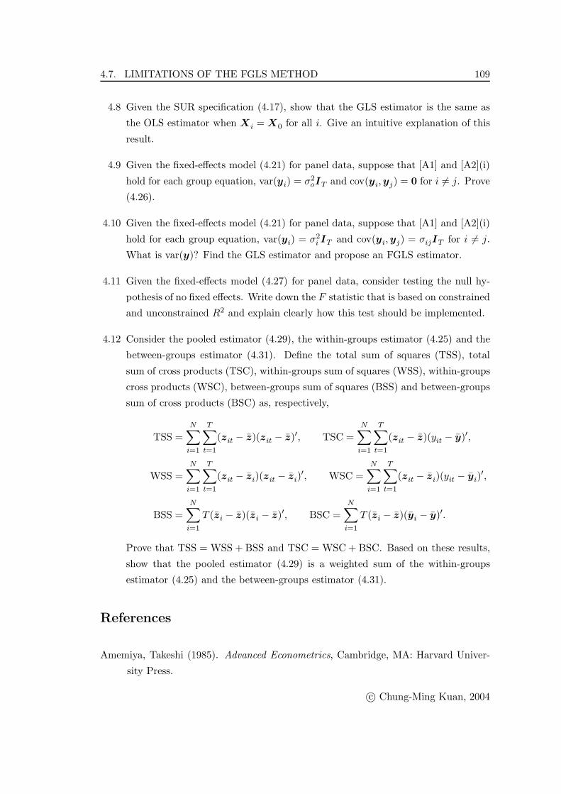
4.8 Given the SUR specification (4.17), show that the GLS estimator is the same as

the OLS estimator when Xi = X0 for all i. Give an intuitive explanation of this

result.

4.9 Given the fixed-effects model (4.21) for panel data, suppose that [A1] and [A2](i)

hold for each group equation, var(yi) = σ2oIT and cov(yi,yj) = 0 for i �= j. Prove

(4.26).

4.10 Given the fixed-effects model (4.21) for panel data, suppose that [A1] and [A2](i)

hold for each group equation, var(yi) = σ2i IT and cov(yi,yj) = σijIT for i �= j.

What is var(y)? Find the GLS estimator and propose an FGLS estimator.

4.11 Given the fixed-effects model (4.27) for panel data, consider testing the null hy-

pothesis of no fixed effects. Write down the F statistic that is based on constrained

and unconstrained R2 and explain clearly how this test should be implemented.

4.12 Consider the pooled estimator (4.29), the within-groups estimator (4.25) and the

between-groups estimator (4.31). Define the total sum of squares (TSS), total

sum of cross products (TSC), within-groups sum of squares (WSS), within-groups

cross products (WSC), between-groups sum of squares (BSS) and between-groups

sum of cross products (BSC) as, respectively,

TSS =N∑

i=1

T∑t=1

(zit − z)(zit − z)′, TSC =N∑

i=1

T∑t=1

(zit − z)(yit − y)′,

WSS =N∑

i=1

T∑t=1

(zit − zi)(zit − zi)′, WSC =

N∑i=1

T∑t=1

(zit − zi)(yit − yi)′,

BSS =N∑

i=1

T (zi − z)(zi − z)′, BSC =N∑

i=1

T (zi − z)(yi − y)′.

Prove that TSS = WSS + BSS and TSC = WSC + BSC. Based on these results,

show that the pooled estimator (4.29) is a weighted sum of the within-groups

estimator (4.25) and the between-groups estimator (4.31).

References

Amemiya, Takeshi (1985). Advanced Econometrics, Cambridge, MA: Harvard Univer-

sity Press.



Farebrother, R. W. (1980). The Durbin-Watson test for serial correlation when there is

no intercept in the regression, Econometrica, 48, 1553–1563.

Goldberger, Arthur S. (1991). A Course in Econometrics, Cambridge, MA: Harvard

University Press.

Greene, William H. (2000). Econometric Analysis, Fourth ed., New York, NY: Macmil-

lan.

Wallis, K. F. (1972). Testing for fourth order autocorrelation in quarterly regression

equations, Econometrica, 40, 617–636.


generalized least squares theory

Documents