generalized linear model - imperial college londonbm508/teaching/appstats/lecture5.pdfgeneralized...

Generalized Linear Model

Badr Missaoui

Logistic Regression

OutlineI Generalized linear modelsI DevianceI Logistic regression.


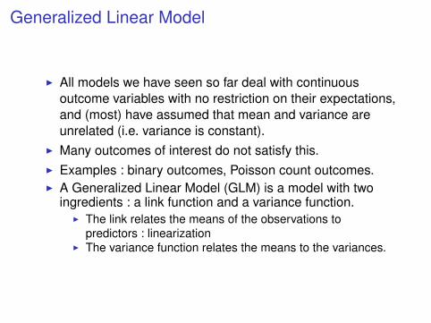
I All models we have seen so far deal with continuousoutcome variables with no restriction on their expectations,and (most) have assumed that mean and variance areunrelated (i.e. variance is constant).

I Many outcomes of interest do not satisfy this.I Examples : binary outcomes, Poisson count outcomes.I A Generalized Linear Model (GLM) is a model with two

ingredients : a link function and a variance function.I The link relates the means of the observations to

predictors : linearizationI The variance function relates the means to the variances.


I The data involve 462 males between the ages of 15 and64. The outcome Y is the presence (Y = 1) or absenceY = 0 of heart diseaseCoefficients:

Estimate Std. Error z value Pr(>|z|)(Intercept) -5.9207616 1.3265724 -4.463 8.07e-06 ***sbp 0.0076602 0.0058574 1.308 0.190942tobacco 0.0777962 0.0266602 2.918 0.003522 **ldl 0.1701708 0.0597998 2.846 0.004432 **adiposity 0.0209609 0.0294496 0.712 0.476617famhistPresent 0.9385467 0.2287202 4.103 4.07e-05 ***typea 0.0376529 0.0124706 3.019 0.002533 **obesity -0.0661926 0.0443180 -1.494 0.135285alcohol 0.0004222 0.0045053 0.094 0.925346age 0.0441808 0.0121784 3.628 0.000286 ***


MotivationI Classical linear model

Y = Xβ + ε

where ε ∼ N(0, σ2). That means,

Y ∼ N(Xβ, σ2)

I In the GLM, we specify that

Y ∼ P(Xβ)


We write the GLM asE(Yi) = µi

andηi = g(µi) = Xiβ

where the function g called a link function which belongs to anexponential family.


I The exponential family density are specifying twocomponents, the canonical parameter θ and the dispersionparameter φ .

I Let Y = (Yi)i=1...n be a sequence of random variables. Yihas an exponential density if

fYi (yi ; θi , φ) = exp(

yiθi − b(θi)

ai(φ)+ c(yi , φ)

)where the functions b, c are specific to each distributionand ai(φ) = φ/wi .


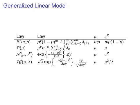
Law Law µ σ2

B(m,p) py (1− p)m−y .(m

y

)∑mk=0 δ{k} mp mp(1− p)

P(µ) µye−µ.∑m

k=01k!δk µ µ

N (µ, σ2) exp{− (y−µ)2

2σ2

}.dy µ σ2

IG(µ, λ)√λexp

{−λ(y−µ)2

2µy

}. dy√

2πy3µ µ3/λ


I We write`(y ; θ, φ) = log f (y ; θ, φ)

for the log-likelihood function of Y .I Using the facts that

E(∂`

∂θ

)= 0

Var(∂`

∂θ

)= −E

(∂2`

∂θ2

)I We have

E(y) = b′(θ)

andVar(y) = b′′(θ)a(φ)

Generalized Linear ModelI Gaussian case

f (y ; θ, φ) =1

σ√

2πexp

[−(y − µ)2

2σ2

]= exp

(yµ− µ2/2

σ2 − 12

(y2

σ2 + log(2πσ2)

))We can write θ = µ, φ = σ2, a(φ) = φ, b(θ) = θ2/2 andc(y , φ) = −1

2

(y2

σ2 + log(2πσ2))

I Binomial case

f (y ; θ, φ) =

(ny

)µy (1− µ)n−y

= exp(

y log(

µ

1− µ

)+ n log(1− µ) + log

(ny

))We can write θ = log µ

1−µ , b(θ) = −n log(1− µ) andc(y , φ) = log

(ny

)


Recall that in ordinary linear models, the MLE of β satisfies

β = (X T X )−1X T Y

if X has full rank.In GLM, the MLE β does not exist in closed form and can beapproximately estimated via iterative weighted least squares.

Generalized Linear ModelI For n observations, the log-likelihood function is

L(β) =n∑

i=1

`(yi ; θ, φ)

I Computing∂`i∂βj

=∂`i∂θi

∂θi

∂µi

∂µi

∂ηi

∂ηi

∂βj= xij

1g′(µi)

1b′′(θi)

yi − µi

φ/wi

I The likelihood equations are

∂Li

∂βj=

n∑i=1

xij1

g′(µi)2Var(yi)

∂µi

∂ηi(yi − µi) = 0 j = 1, ..,p

I PutW = diag

{g′(µi)

2Var(yi)}

i=1,...,n

and∂µ

∂η= diag

{∂µi

∂ηi

}i=1,...,n


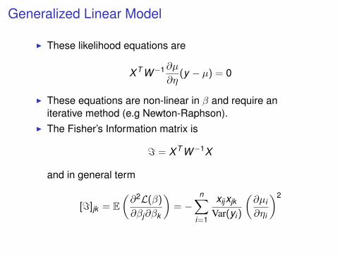
I These likelihood equations are

X T W−1∂µ

∂η(y − µ) = 0

I These equations are non-linear in β and require aniterative method (e.g Newton-Raphson).

I The Fisher’s Information matrix is

= = X T W−1X

and in general term

[=]jk = E(∂2L(β)∂βj∂βk

)= −

n∑i=1

xijxjk

Var(yi)

(∂µi

∂ηi

)2


Let µ0 = Y be the initial estimate. Then, set η0 = g(µ0),and form the adjusted variable

Z 0 = η0 + (Y − µ0)∂η

∂µ|µ=µ0

Calculate β1 by the least squares regression of Z 0 on X ,that means

β1 = argminβ(Z 0 − Xβ)T W−10 (Z 0 − Xβ)

So,β1 = (X T W−1

0 X )−1X T W−10 Z 0

Setη1 = X β1, µ1 = g−1(η1)

Repeat until changes in βm are sufficiently small.

Generalized Linear ModelEstimation

I In theory, βm → β as m→∞, but in practice, the algorithmmay fail to converge.

I Under some conditions,

β → N(β,=−1(β))

I In practice, the asymptotic covariance matrix of β isestimated by

φ(X T W−1m X )−1

where Wm is the weight matrix from the mth iteration.I If φ is unknown, it is estimated by

φ =1

n − p

n∑i=1

wi(yi − µ)2

V (µ)

where V (µi) = var(yi)/a(φ) = wivar(yi)/φ

Generalized Linear ModelI Confidence interval

CIα(βi) =

[βj − u1−α/2

1√nσβj ; βj + u1−α/2

1√nσβj

]where u1−α/2 is the 1− α/2 quantile of N(0,1) and

σβj =1n

[=(β)

]−1

jj.

I To test the hypothesis

H0 : βj = 0 against H1 : βj 6= 0

|βj |√φ(X T W−1

m X )−1(j , j)∼ N(0,1)

if φ is unknown

|βj |√φ(X T W−1

m X )−1(j , j)∼ tn−p


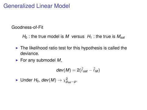
Goodness-of-Fit

H0 : the true model is M versus H1 : the true is Msat

I The likelihood ratio test for this hypothesis is called thedeviance.

I For any submodel M,

dev(M) = 2(ˆsat − ˆM)

I Under H0, dev(M)→ χ2psat−p.


Goodness-of-FitI The scaled deviance for GLM is

D(y , µ) = 2 [`(µsat , φ; y)− `(µ, φ; y)]

=n∑

i=1

2wi{

yi(θ(µsati )− θ(µi))− b(µsat

i ) + b(µi}/φ

=n∑

i=1

D?(yi ; µi)/φ

= D?(y ; µ)/φ


TestsI We use the deviance to compare two models having p1

and p2 parameters respectively, where p1 < p2. Let µ1 andµ2 denote the corresponding MLEs.

I

D(y , µ1)− D(y , µ2) ∼ χ2p2−p1

I If φ is unknown,

D?(y , µ1)− D?(y , µ2)

(p2 − p1)φ∼ F1−α,p2−p1,n−p2


Goodness-of-FitI The deviance residuals for a given model are

di = sign(yi − µi)√

D?(yi ; µi)

I A poorly fitting point will make a large contribution to thedeviance, so |di | will be large.


DiagnosticsI The Pearson residuals are defined by

ri =yi − µi√

(1− hii)V (µ)

where hii is the ith diagonal element of

H = X (X T W−1m X )−1X T W−1

m

I The deviance residuals are

εi = sign(yi − µi)

√D?(yi ; µi)

1− hii


DiagnosticsI The Anscombe residuals is defined as a transformation of

the Pearson residual

rAi =

t(yi)− t(µi)

t ′(µi)√φV (µi)(1− hii)

The aim in introducing the function t is to make theresiduals as Gaussian as possible. We consider

t(x) =∫ x

0V (µ)−1/3dµ


DiagnosticsI Influential points using the Cook’s distance

Ci =1p(β(i) − β)T X T WmX (β(i) − β) ≈ r2

ihii

p(1− hii)2

I The outliers points : if hii > 2p/n or hii > 3p/n, then weconsider that ith point is an outlier.


Model SelectionI Model selection can be done using the AIC and BIC.I Forward, Backward and stepwise approach can be used.


Logistic regressionI Logistic regression is a generalization of regression that is

used when the outcome Y is binary 0,1.I As example, we assume that

P(Yi = 1|Xi) =eβ0+β1Xi

1 + eβ0+β1Xi

I Note thatE(Yi |Xi) = P(Yi = 1|Xi)


Logistic regressionI Define the logit function

logit(z) = log(

z1− z

)I We can write

logit(πi) = β0 + β1Xi

where πi = P(Yi = 1|Xi)

I The extension to several covariates is

logit(πi) = β0 +

p∑i=1

βjxij


How do we estimate the parameters ?I Can be fit using maximum likelihood.I The likelihood function is

L(β) =n∏

i=1

f (yi |Xi ;β) = L(β) =n∏

i=1

πyii (1− πi)

1−yi

I The estimator β has to be found numerically.


Usually, we use the reweighted least squaresI First set a starting values of β(0)

I Compute

πi =eXiβ

(k)

1 + eX iβ(k)

I Define weighted matrix W whose i th diagonal is πi(1− πi)

I Define the adjusted response vectorZ = Xβ(k) + W−1(Y − π)

I Takeβ(k+1) = (X T WX )−1X T WZ

which is the weighted linear regression of Z on X


Model selection and diagnosticsI Diagnostics : the Pearson χ2

Yi − πi√πi(1− πi)

I The deviance residuals

sign(Yi − πi)

√2[Yi log

(Yi

πi

)+ (1− Yi) log

(1− Yi

1− πi

)]

Generalized Linear ModelI To fit this model, we use the glm command.

Call:glm(formula = chd ~ ., family = binomial, data = SAheart)

Deviance Residuals:Min 1Q Median 3Q Max

-1.8320 -0.8250 -0.4354 0.8747 2.5503

Coefficients:Estimate Std. Error z value Pr(>|z|)

(Intercept) -5.9207616 1.3265724 -4.463 8.07e-06 ***row.names -0.0008844 0.0008950 -0.988 0.323042sbp 0.0076602 0.0058574 1.308 0.190942tobacco 0.0777962 0.0266602 2.918 0.003522 **ldl 0.1701708 0.0597998 2.846 0.004432 **adiposity 0.0209609 0.0294496 0.712 0.476617famhistPresent 0.9385467 0.2287202 4.103 4.07e-05 ***typea 0.0376529 0.0124706 3.019 0.002533 **obesity -0.0661926 0.0443180 -1.494 0.135285alcohol 0.0004222 0.0045053 0.094 0.925346age 0.0441808 0.0121784 3.628 0.000286 ***---Signif. codes: 0 *** 0.001 ** 0.01 * 0.05 . 0.1 1

(Dispersion parameter for binomial family taken to be 1)

Null deviance: 596.11 on 461 degrees of freedomResidual deviance: 471.16 on 451 degrees of freedomAIC: 493.16

Number of Fisher Scoring iterations: 5


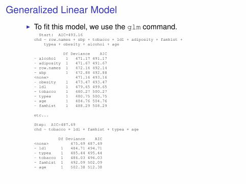
I To fit this model, we use the glm command.Start: AIC=493.16

chd ~ row.names + sbp + tobacco + ldl + adiposity + famhist +typea + obesity + alcohol + age

Df Deviance AIC- alcohol 1 471.17 491.17- adiposity 1 471.67 491.67- row.names 1 472.14 492.14- sbp 1 472.88 492.88<none> 471.16 493.16- obesity 1 473.47 493.47- ldl 1 479.65 499.65- tobacco 1 480.27 500.27- typea 1 480.75 500.75- age 1 484.76 504.76- famhist 1 488.29 508.29

etc...

Step: AIC=487.69chd ~ tobacco + ldl + famhist + typea + age

Df Deviance AIC<none> 475.69 487.69- ldl 1 484.71 494.71- typea 1 485.44 495.44- tobacco 1 486.03 496.03- famhist 1 492.09 502.09- age 1 502.38 512.38


I Suppose Yi ∼ Binomial(ni , πi)

I We can fit the logistic model as before

logit(πi) = Xiβ

I Pearson residuals

ri =Yi − ni πi√ni πi(1− πi)

I Deviation residuals

di = sign(Yi−Yi)

√2[Yi log

(Yi

µi

)+ (ni − Yi) log

(ni − Yi

ni − µi

)]


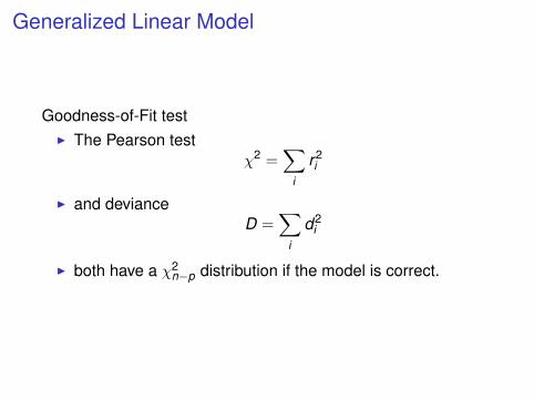
Goodness-of-Fit testI The Pearson test

χ2 =∑

i

r2i

I and devianceD =

∑i

d2i

I both have a χ2n−p distribution if the model is correct.


I To fit this model, we use the glm command.Call:glm(formula = cbind(y, n - y) ~ x, family = binomial)

Deviance Residuals:Min 1Q Median 3Q Max

-0.70832 -0.29814 0.02996 0.64070 0.91132

Coefficients:Estimate Std. Error z value Pr(>|z|)

(Intercept) -14.73119 1.83018 -8.049 8.35e-16 ***x 0.24785 0.03031 8.178 2.89e-16 ***---Signif. codes: 0 *** 0.001 ** 0.01 * 0.05 . 0.1 1

(Dispersion parameter for binomial family taken to be 1)

Null deviance: 137.7204 on 7 degrees of freedomResidual deviance: 2.6558 on 6 degrees of freedomAIC: 28.233

Number of Fisher Scoring iterations: 4


To test the correctness of the model> pvalue = 1-pchisq(out$dev,out$df.residual)> print(pvalue)[1] 0.8506433> r=resid(out,type="deviance")> p=out$linear.predictors> plot(p,r,pch=19,xlab="linear predictor", ylab="deviance residuals")> print(sum(r^2))[1] 2.655771> cooks.distance(out)

1 2 3 4 50.0004817501 0.3596628502 0.0248918197 0.1034462077 0.02429419426 7 8

0.0688081629 0.0014847981 0.0309767612

Note that the residuals give back the deviance test, and thep-value is large indicating no evidence of a lack of fit.

generalized linear model - imperial college londonbm508/teaching/appstats/lecture5.pdfgeneralized...

Documents