generalized parton distributions of the photon - bltp …theor.jinr.ru/~spin/2013/talks/nair.pdf ·...

Generalized Parton Distributions of the Photon

Sreeraj Nair

In collaboration with Prof.Asmita Mukherjee,Vikash.K.Ojha

IIT Bombay

October 10, 2013

Sreeraj Nair (IIT Bombay) DSPIN 2013,DUBNA Sreeraj Nair, IIT BombayOctober 10, 2013 0 / 25

Outline

1 Introduction to Proton GPDs

2 How and Why GPDs

3 Photon GPDs

4 Helicity Flip Photon GPDs

5 Conclusion

Defination of Proton GPDs

They are defined as off-forward matrix elements of well defined field operators in

between proton states having different momenta.

Fλ,λ′ =

∫

dy−

8πeixP+y−/2〈P′, λ′| Ψ(0) γ+Ψ(y) |P, λ〉

∣

∣

∣

y+=0,y⊥=0

=1

2P+U(P′, λ′)

[

H(x, ζ, t) γ+ + E(x, ζ, t)iσ+α(−∆α)

2M

]

U(P, λ)

Fλ,λ′ =

∫

dy−

8πeixP

+y−/2〈P′, λ′| Ψ(0) γ+γ5Ψ(y) |P, λ〉

∣

∣

∣

y+=0,y⊥=0

=1

2P+U(P′, λ′)

[

H(x, ζ, t) γ+γ5 + E(x, ζ, t)γ5(−∆+)

2M

]

U(P, λ)

x ⇒ fractional momentum carried by the active quark.

ζ =Q2

2P.q⇒ skewness variable.

∆ = P − P′ ⇒ Momentum transfer from intial target state to final state (t = ∆2)


Basic properties of GPDs

In the forward limit (p = p′, t = 0) :

Hq(x, 0, 0) = q(x), Hq(x, 0, 0) = ∆q(x) for x > 0,

Hq(x, 0, 0) = −q(−x), Hq(x, 0, 0) = ∆q(−x) for x < 0.

Connection to elastic FFs :

∫ 1

−1

dxHq(x, ξ, t) = Fq

1(t),

∫ 1

−1

dxEq(x, ξ, t) = Fq

2(t),

∫ 1

−1

dxHq(x, ξ, t) = gqA(t),

∫ 1

−1

dxEq(x, ξ, t) = gqP(t)

where, Fq

1(t) and Fq

2(t) are the Dirac and Pauli FFs respectively.

gqA(t) and g

qP(t) are the axial and psedoscalar FFs respectively.

ζ =2ξ

1 + ξ


Outline


2 How and Why GPDs

3 Photon GPDs


5 Conclusion

Deeply Virtual Compton Scattering(DVCS) on a Proton

target

Exclusive Process ⇒ All final states are known.

The final and intial state momenta are different:

P =(

P+,−→0 ⊥,

M2

P+

)

P′ =(

(1 − ζ)P+,−∆⊥,M2 +∆2

⊥

(1 − ζ)P+

)

momentum transfer ⇒ ∆ = P − P′

LC co-ordinates ⇒ V± = V0 ± Vz

V2 = V+V− − (V⊥)2

Final state has a real photon

γ∗(q) + p(P) → γ(q′) + p(P′)

γ∗

γ

e−

e−

p p′

GPD

ep → epγ

Factorization of DVCS amplitude

hard part → perturbative

soft part → generalised parton

distributions(GPD)

X. Ji, PRL, 1997


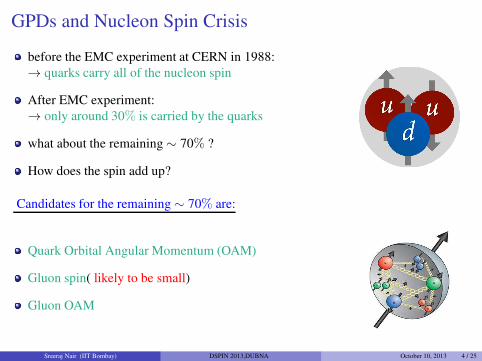
GPDs and Nucleon Spin Crisis

before the EMC experiment at CERN in 1988:

→ quarks carry all of the nucleon spin

After EMC experiment:

→ only around 30% is carried by the quarks

what about the remaining ∼ 70% ?

How does the spin add up?

Candidates for the remaining ∼ 70% are:

Quark Orbital Angular Momentum (OAM)

Gluon spin( likely to be small)

Gluon OAM


GPDs and spin sum rule

Second moment of the GPDs gives the fraction of the nucleon spin carried by the

quarks

Jq is accessible through GPDs:

1

2

∫ 1

0

dx x

[

Hq(x, 0, 0) + Eq(x, 0, 0)]

= Jq(Q2)

∑

q

Jq + Jg =1

2X.Ji, 1997

DVCS to probe Jq = Sq + Lq

but no further decomposotion of Jg


Outline


2 How and Why GPDs

3 Photon GPDs


5 Conclusion

Generalized parton distributions of the photon

The partonic constituents of the photon play a dominant role when the virtuality

Q2 is very large. Photon sturucture function are well understood both

theoretically and experimentally.

DVCS on a photon target ⇒ γ∗γ → γγ in the kinematic region of large

center-of-mass energy,large virtuality(Q2) but small squared momentum transfer

(−t)

At leading order in α and zeroth order in αs the result for the amplitude was

interpreted to be factorized and upto leading log terms was written in terms of

the GPDs of the photon.

S. Friot, B. Pire, L. Szymanowski, PLB 645 153 (2007)

R. Gabdrakhmanov, O.V. Teryaev, PLB 716 417 (2012)

The momentum transfer from the intial to final state(∆) is purely in the

longitudnal direction(∆⊥ = 0)


Defination of Photon GPDs

The GPDs of the photon can be expressed as the following off-forward matrix

elements defined for real photon target state

Fq =

∫

dy−

8πe

−iP+y−

2 〈γ(P′), λ′ | ψ(0)γ+ψ(y−) | γ(P), λ〉

Fq =

∫

dy−

8πe

−iP+y−

2 〈γ(P′), λ′ | ψ(0)γ+γ5ψ(y−) | γ(P), λ〉

here | γ(P), λ〉 is the (real) photon target state of momentum P and helicity λ.

Fq → contibutes when photon is unpolarised

Fq → photon is polarised

light front gauge chosen → A+ = 0

Fq can be calculated from the terms of the form ǫ2λǫ

1∗λ − ǫ1

λǫ2∗λ


Photon GPD as Overlap of LFWFs

We calculate the Photon GPDs for ∆⊥ 6= 0 and also for skewness ζ 6= 0

Fq and Fq can be calculated using the Fock space expansion of the photon state:

| γ(P)〉 =√

N[

a†(P, λ) | 0〉+∑

σ1,σ2

∫

{dk1}∫

{dk2}√

2(2π)3P+δ3(P − k1 − k2)

φ2(k1, k2, σ1, σ2)b†(k1, σ1)d

†(k2, σ2) | 0〉]

where, {dk} =

∫

dk+d2k⊥√

2(2π)3k+

,

φ2 is the two-particle (qq) light-front wave function (LFWF) and σ1 and σ2 are

the helicities of the quark and antiquark


Photon GPD as Overlap of LFWFs

DVCS amplitude is given in terms of overlaps of the light-front wave functions.

Diehl, Feldman, Jakob, Kroll; Nucl. Phys. B (2001);

Brodsky, Diehl, Huang; Nucl. Phys. B (2001).

Fq =

∫

d2q⊥dx1δ(x − x1)ψ∗λ′

2 (x1, q′⊥)ψλ

2 (x1, q⊥) 1 > x > 0

The two-particle LFWFs for the photon are given by

ψλ2s1,s2

(x, q⊥) =1

m2 − m2+(q⊥)2

x(1−x)

eeq√

2(2π)3χ†

s1

[ (σ⊥ · q⊥)

xσ⊥

−σ⊥ (σ⊥ · q⊥)

1 − x− i

m

x(1 − x)σ⊥]

χ−s2ǫ⊥∗λ

where m is the mass of q(q). λ is the helicity of the photon and s1, s2 are the

helicities of the q and q respectively.

A.Harindranath,R.Kundu,A.Mukherjee, PRD 59, 094013,(1999).


Kinematics

Chosen frame of refrence: Brodsky, Diehl, Huang; Nucl. Phys. B (2001)

P =(

P+ , 0⊥ , 0)

,

P′ =

(

(1 − ζ)P+ , −∆⊥ ,∆⊥2

(1 − ζ)P+

)

,

The four-momentum transfer from the target is:

∆ = P − P′ =

(

ζP+ , ∆⊥ ,t +∆⊥2

ζP+

)

,

where t = ∆2 and ζ is called the skewness variable. In addition, overall

energy-momentum conservation requires ∆− = P− − P′−

which connects ∆⊥2, ζ, and t according to

(1 − ζ)t = −∆⊥2.


Photon GPD for ζ = 0

Fq =∑

q

αe2q

4π2

[

((1 − x)2 + x2)(I1 + I2 + LI3) + 2m2I3

]

1 > x > 0

Fq =∑

q

αe2q

4π2

[

(x2 − (1 − x)2)(I1 + I2 + LI3) + 2m2I3

]

1 > x > 0

where L = −2m2 + 2m2x(1 − x)− (∆⊥)2(1 − x)2

I1 = πLog

[ Λ2

µ2 − m2x(1 − x) + m2

]

= I2

I3 =

∫ 1

0

dαπ

P(x, α, (∆⊥)2)

P(x, α, (∆⊥)2) = −m2x(1 − x) + m2 + α(1 − α)(1 − x)2(∆⊥)

2.


Photon GPD for ζ = 0

0 0.2 0.4 0.6 0.8 1

x

0.2

0.4

0.6

0.8

1

1.2

Fq

-t = 0.0-t = 0.01-t = 0.1-t = 1.0-t = 3.0

0 0.2 0.4 0.6 0.8 1

x

-1

-0.5

0

0.5

1

Fq~

-t = 0.0-t = 0.01-t = 0.1-t = 1.0-t = 3.0

A.Mukherjee,S.Nair, PLB 706, (2011) 77-81

We fixed Q = Λ = 20GeV , m = 3.3MeV

As x → 1 most of the momentum is carried by the quark in the photon and the

GPDs become independent of t


Photon GPDs in impact parameter space(IPS)

Fourier transform with respect to the transverse momentum transfer ∆⊥ we get the

GPDs in the transverse impact parameter space.

q(x, b⊥) =1

(2π)2

∫

d2∆⊥e−i∆⊥·b⊥Fq =1

2π

∫

∆d∆J0(∆b)Fq

q(x, b⊥) =1

(2π)2

∫

d∆e−i∆⊥·b⊥ Fq =1

2π

∫

∆d∆J0(∆b)Fq

probability of finding a quark of momentum fraction x and at transverse distance

b from the center of the photon : parton distributions of the photon in the

transverse plane.

New insight to the transverse ’shape’ of the photon

J0(z) is the Bessel function; ∆ = |∆⊥| and b = |b⊥|.


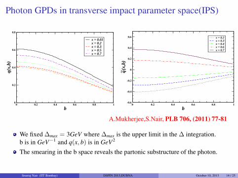
Photon GPDs in transverse impact parameter space(IPS)

0 0.2 0.4 0.6 0.8 1

b0

0.2

0.4

0.6

0.8

q(x,

b)

x = 0.01x = 0.2x = 0.3x = 0.5x = 0.7

0 0.2 0.4 0.6 0.8 1

b-0.6

-0.4

-0.2

0

0.2

0.4

0.6

q~(x

,b)

x = 0.2x = 0.3x = 0.4x = 0.6x = 0.7


We fixed ∆max = 3GeV where ∆max is the upper limit in the ∆ integration.

b is in GeV−1 and q(x, b) is in GeV2

The smearing in the b space reveals the partonic substructure of the photon.


Photon GPDs for ζ 6= 0

We again calculate Fq and Fq when ζ and ∆⊥ both are non-zero

We consider only the kinematical region 1 > x > ζ and −1 < x < ζ − 1 where

only the two particle LFWFs contribute

When the skewness ζ is non-zero, GPDs in impact parameter space do not have a

probabilistic interpretation

They are still interesting as they now probe the partons when the initial photon is

displaced from the final photon in the transverse impact parameter space. This

relative shift does not vanish when the GPDs are integrated over x in the

amplitude Diehl(2002)


Photon GPDs for ζ 6= 0

0.2 0.4 0.6 0.8 1

x

0.2

0.4

0.6

0.8

1

Fq

-t = 0.1-t = 1.0-t = 3.0-t = 5.0

ζ = 0.1

0.2 0.4 0.6 0.8 1

x

-0.5

0

0.5

1

Fq~

-t = 0.1-t = 1.0-t = 3.0-t = 5.0

ζ = 0.1


We fixed Λ = 20GeV and m = 3.3MeV

x is positive and x > ζ so only the active quark in the photon contributes.


GPDs in longitudinal impact parameter space(IPS)

The Fourier transform of the DVCS amplitude with respect to the skewness

parameter ζ can be used to provide an image of the target hadron in the

boost-invariant variable σ

S. J. Brodsky, D. Chakrabarti, A. Harindranath, A. Mukherjee and J. P. Vary,

Phys. Lett. B 641, 440 (2006)

Phys. Rev. D 75, 014003 (2007).

DVCS amplitude shows a diffraction pattern in longitudinal impact parameter

space.

GPDs for the proton when expressed in term of σ also exhibit the similar

diffraction pattern.

R. Manohar, A. Mukherjee, D. Chakrabarti, Phys.Rev.D83, 014004,(2011).


Photon GPDs in longitudinal impact parameter space(IPS)

we introduce the boost invariant longitudinal impact parameter conjugate to the

longitudinal momentum transfer as σ =1

2b−P+

q(x, σ, t) =1

2π

∫ ζmax

0

dζeiζP+b−/2Fq(x, ζ, t) =1

2π

∫ ζmax

0

dζeiζσFq(x, ζ, t)

-30 -20 -10 0 10 20 30

σ0

0.01

0.02

0.03

0.04

0.05

0.06

q(x,

σ,t)

-t = 0.1

-t = 1.0

-t = 3.0

-t = 5.0

x = 0.4

-30 -20 -10 0 10 20 30

σ0

0.01

0.02

0.03

0.04

q~ (x,σ

,t)

-t = 0.1

-t = 1.0

-t = 3.0

-t = 5.0

x = 0.4


the finite range of ζ integration acts as a slit of finite width necessary to produce

the diffraction pattern.


Outline


2 How and Why GPDs

3 Photon GPDs


5 Conclusion

Helicity flip photon GPD

Transverse polarization vector of photon ⇒ ǫ⊥± =1√2(∓1,−i)

non-vanishing contributions ⇒ (ǫ1+1ǫ

1∗−1 + ǫ2

+1ǫ2∗−1) ⇒ E1

⇒ (ǫ1+1ǫ

1∗−1 − ǫ2

+1ǫ2∗−1) ⇒ E2 (related to E1 by phase

change in ∆⊥ plane)

The GPD with helicity flip is given by :

E1 =αe2

q

2πx(1 − x)3((∆1)

2 − (∆2)2)[

∫ 1

0

dq

B(q)((1 − q)2 − (1 − q))

]

.

where

B(q) = m2(

1 − x(1 − x))

+ q(1 − q)(1 − x)2(∆⊥)2.


Photon GPD E1 in Impact Parameter Space(IPS)

We define the parton distributions with the helicity flip of the photon in transverse

impact parameter space as:

q1(x, b⊥) =

1

4π2

∫

d2∆⊥e−i∆⊥·b⊥E1(x,∆⊥)

where b⊥ is the transverse impact parameter conjugate to ∆⊥.

We then get

q1(x, b⊥) =

1

2π

∫ ∞

0

∆d∆1

π

∫ π

0

(P2(b,∆, θ)− P1(b,∆, θ))dθ f (x)Q(x, t)

Using the intergal representation of the Bessel function J0(x)


where

P2(b,∆, θ) = − 1

b3∆sinθ

[

(b2)2b∆cos

(

b∆sinθ)

sinθ +

(b1)2sin(

b∆sinθ)]

P1(b,∆, θ) = − 1

b3∆sinθ

[

(b1)2b∆cos

(

b∆sinθ)

sinθ +

(b2)2sin(

b∆sinθ)]

.

f (x) =αe2

q

2πx(1 − x)3 and Q(x, t) =

∫ 1

0

dq

B(q)((1 − q)2 − (1 − q)).


x-dependence of E1(x,∆⊥) and q1(x, b⊥)

φ = tan−1∆2

∆1β = tan−1 b2

b1

0.0 0.2 0.4 0.6 0.8 1.00.00

0.05

0.10

0.15

0.20

0.25

0.30

Φ = 60o

x

E1Hx

,D¦

L

-t=5.0

-t=3.0

-t=1.0

-t=0.1

0.0 0.2 0.4 0.6 0.8 1.00.0

0.2

0.4

0.6

0.8

1.0

1.2

Β = 30o

xq 1Hx

,b¦

L b = 0.8

b = 0.6

b = 0.4

b = 0.2

A.Mukherjee,S.Nair,V.K.Ojha, PLB 721, (2013) 284-289

At x = 0 and x = 1 all momenta are carried by either the quark or the anti-quark

in the photon. Then there is no relative motion and no OAM contribution.

q1(x, b⊥) is maximum when x = 0.5, that is when the quark and the anti-quark

carry equal momentaSreeraj Nair (IIT Bombay) DSPIN 2013,DUBNA Sreeraj Nair, IIT BombayOctober 10, 2013 22 / 25

∆max dependence of q1(x, b⊥)

Plots of q1(x, b⊥) vs. b1, b2 for different values of ∆max. b1 and b2 are in GeV−1 and

∆max is in GeV. x = 0.3


q1(x, b⊥) has a quadrupole structure, that comes because it involves a helicity

flip of a spin one object (photon)



as ∆max increases the peaks become sharper, which means that the distortion in

b⊥ space moves closer to the origin.


Outline


2 How and Why GPDs

3 Photon GPDs


5 Conclusion

Conclusion

We have calculated the GPDs of the photon,both polarised and unpolarised,when

the momentum transfer is non-zero in the longitudinal as well as transverse

direction at zeroth order in αs and leading order in α.

Taking the fourier transform with respect to ∆⊥ we obtain impact parameter

dependent parton distribution of the photon.

Photon GPDs in longitudinal position space show interesting pattern similar to

the diffraction pattern in optics.

For the helicity flip case the Photon GPDs has a quadrupole structure and gets

the contribution from the non-zero orbital angular momentum of the photon

light-front wave function.

The GPDs of the photon calculated here may act as interesting tools to

understand the partonic substructure of the photon. Accessing them in

experiment is a challenge.


Thank You All For Listening

Special Thanks to Prof. Oleg Teryaev for arranging the

financial support for my extended stay.

BACKUP SLIDES

0 0.2 0.4 0.6 0.8 1

x0

0.5

1

1.5

2

q(x,

b)

b = 0.1b = 0.3b = 0.6b = 0.7b = 0.8

0 0.2 0.4 0.6 0.8 1

b0

0.2

0.4

0.6

0.8

q(x,

b)

x = 0.01x = 0.2x = 0.3x = 0.5x = 0.7

We fixed ∆max = 3GeV where ∆max is the upper limit in the ∆ integration.

b is in GeV−1 and q(x, b) is in GeV2

The smearing in the b space reveals the partonic substructure of the photon.

BACKUP SLIDES

0 0.2 0.4 0.6 0.8 1

x

-0.5

0

0.5

1

1.5

2

q~(x

,b)

b = 0.2

b = 0.3

b = 0.6

b = 0.7

b = 0.8

0 0.2 0.4 0.6 0.8 1

b-0.6

-0.4

-0.2

0

0.2

0.4

0.6

q~(x

,b)

x = 0.2x = 0.3x = 0.4x = 0.6x = 0.7

The behavior in impact parameter space is qualitatively different from

phenomenological models of proton GPDs

Parton distribution is more dispersed when the q and q share almost equal

momenta

BACKUP SLIDES

0 0.2 0.4 0.6 0.8 1

b0

0.1

0.2

0.3

0.4

0.5

0.6

q(x,

ζ,b)

x = 0.2x = 0.4x = 0.6x = 0.8

ζ = 0.1

0 0.2 0.4 0.6 0.8 1

b

-0.4

-0.2

0

0.2

0.4

q~(x

,ζ ,b

)

x = 0.2x = 0.3x = 0.4x = 0.6x = 0.7

ζ = 0.1

BACKUP SLIDES

-30 -20 -10 0 10 20 30

σ0

0.01

0.02

0.03

0.04

0.05

0.06

0.07

q(x,

σ,t)

-t = 0.1

-t = 1.0

-t = 3.0

-t = 5.0

x = 0.5

-30 -20 -10 0 10 20 30

σ0

0.005

0.01

0.015

0.02

0.025

0.03

q~(x

,σ,t)

-t = 0.1

-t = 1.0

-t = 3.0

-t = 5.0

x = 0.5

BACKUP SLIDES

-30 -20 -10 0 10 20 30

σ0

0.02

0.04

0.06

0.08

q(x,

σ,t)

-t = 0.1

-t = 1.0

-t = 3.0

-t = 5.0

x = 0.6

-30 -20 -10 0 10 20 30

σ0

0.005

0.01

0.015

0.02

q~(x

,σ,t)

-t = 0.1

-t = 1.0

-t = 3.0

-t = 5.0

x = 0.6

BACKUP SLIDES

-30 -20 -10 0 10 20 30

σ0

0.03

0.06

0.09

0.12

0.15

q(x,

σ,t)

-t = 0.1

-t = 1.0

-t = 3.0

-t = 5.0

x = 0.8

-30 -20 -10 0 10 20 30

σ0

0.03

0.06

0.09

0.12

q~(x

,σ,t)

-t = 0.1

-t = 1.0

-t = 3.0

-t = 5.0

x = 0.8

BACKUP SLIDES

-30 -20 -10 0 10 20 30

σ0

0.02

0.04

0.06

0.08

0.1

q(x,

σ,t)

x = 0.1x = 0.2x = 0.3x = 0.4x = 0.5x = 0.6x = 0.7x = 0.8

-t = 3.0

-30 -20 -10 0 10 20 30

σ0

0.01

0.02

0.03

0.04

0.05

0.06

0.07

0.08

q~(x

,σ,t)

x = 0.1x = 0.2x = 0.3x = 0.4x = 0.5x = 0.6x = 0.7x = 0.8

-t = 3.0

BACKUP SLIDESDVCS amplitude is given in terms of overlaps of the light-front wave functions.

Diehl, Feldman, Jakob, Kroll; Nucl. Phys. B (2001);

Brodsky, Diehl, Huang; Nucl. Phys. B (2001).

So the GPDs can be written in terms of the overlaps of the LFWFs as follows :

Fq =

∫

d2q⊥dx1δ(x − x1)ψ∗λ′

2 (x1, q⊥ − (1 − x1)∆

⊥)ψλ2 (x1, q

⊥)

−∫

d2q⊥dx1δ(1 + x − x1)ψ∗λ′

2 (x1, q⊥ + x1∆

⊥)ψλ2 (x1, q

⊥)

The two-particle LFWFs for the photon are given by

ψλ2s1,s2

(x, q⊥) =1

m2 − m2+(q⊥)2

x(1−x)

eeq√

2(2π)3χ†

s1

[ (σ⊥ · q⊥)

xσ⊥

−σ⊥ (σ⊥ · q⊥)

1 − x− i

m

x(1 − x)σ⊥]

χ−s2ǫ⊥∗λ

A. Harindranath, R. Kundu, W. M. Zhang; Phys. Rev. D 59, 094013,(1999).

where m is the mass of q(q). λ is the helicity of the photon and s1, s2 are the helicities

of the q and q respectively.

∆⊥ dependence of E1(x,∆⊥)

Plots of E1(x,∆⊥) vs ∆1,∆2 for fixed values of x and different t.

t is in GeV2. The innermost surface is for the smallest value of −t.

- t = 1.0

- t = 3.0

- t = 5.0

x = 0.05 E1Hx,D¦L - t = 1.0

- t = 3.0

- t = 5.0

x = 0.1 E1Hx,D¦L


E1(x,∆⊥) has a quadrupole structure in ∆⊥ plane coming from the

(∆1)2 − (∆2)

2.


generalized parton distributions of the photon - bltp …theor.jinr.ru/~spin/2013/talks/nair.pdf ·...

Documents