generalized quantum onsager coefficients from a symmetrized campbell-hausdorff expansion

This content has been downloaded from IOPscience. Please scroll down to see the full text.

Download details:

IP Address: 137.30.242.61

This content was downloaded on 10/06/2014 at 12:34

Please note that terms and conditions apply.

Generalized quantum Onsager coefficients from a symmetrized Campbell-Hausdorff

expansion

View the table of contents for this issue, or go to the journal homepage for more

2001 J. Phys. A: Math. Gen. 34 1285

(http://iopscience.iop.org/0305-4470/34/7/305)

Home Search Collections Journals About Contact us My IOPscience

iopscience.iop.org/page/terms

http://iopscience.iop.org/0305-4470/34/7

http://iopscience.iop.org/0305-4470

http://iopscience.iop.org/

http://iopscience.iop.org/search

http://iopscience.iop.org/collections

http://iopscience.iop.org/journals

http://iopscience.iop.org/page/aboutioppublishing

http://iopscience.iop.org/contact

http://iopscience.iop.org/myiopscience

INSTITUTE OF PHYSICS PUBLISHING JOURNAL OF PHYSICS A: MATHEMATICAL AND GENERAL

J. Phys. A: Math. Gen. 34 (2001) 1285–1300 www.iop.org/Journals/ja PII: S0305-4470(01)14081-3

Generalized quantum Onsager coefficients from asymmetrized Campbell–Hausdorff expansion

K Lendi1 and A J van Wonderen2

1 Institute of Physical Chemistry, University of Zurich, Winterthurerstrasse 190, CH-8057 Zurich,Switzerland2 Instituut voor Theoretische Fysica, Universiteit van Amsterdam, Valckenierstraat 65, NL-1018XE Amsterdam, The Netherlands

E-mail: [email protected] and [email protected]

Received 22 May 2000, in final form 21 December 2000

AbstractThe analogue of the classical Onsager theory of entropy production issystematically derived for weakly irreversible processes in open quantumsystems with finite-dimensional Hilbert space. The dynamics is assumedto be given by a quantum dynamical semigroup with infinitesimal generatorof Gorini–Kossakowski–Sudarshan type. The basic Spohn formula forentropy production is used to obtain an expansion in terms of powers ofthe deviation of the initial state relative to the final stationary state ofirreversible dynamics. To this end, an appropriate Lie series is constructedfrom a particular symmetrization procedure applied to the ordinary Campbell–Hausdorff expansion. In this way, only Hermitian contributions by higher-order commutators are generated, which allow an identification with so-called generalized Onsager coefficients. The explicit derivations concentrateon second-, third- and fourth-order coefficients, whereas complete detailedexpressions are worked out for second and third order. In a suitable coherence-vector representation of density matrices the results can be given in terms ofthe dynamical parameters fixing the infinitesimal semigroup generator and interms of symmetric and antisymmetric structure constants of the Lie algebraof SU(N). As an illustration, an application to generalized Bloch equationsfor two-level systems is studied, where the Onsager-like expansion can becompared with exact results for entropy production. We find that convergenceis good even for rather large deviations between initial and final state if thecalculation includes second- and third-order coefficients only. The formalismpresented in this paper generalizes restrictions on admitted final states adoptedin much simpler earlier treatments to the most general case of arbitrary uniquefinal states of irreversible processes.

PACS number: 0570L

0305-4470/01/071285+16$30.00 © 2001 IOP Publishing Ltd Printed in the UK 1285

1286 K Lendi and A J van Wonderen

1. Introduction

Ever since the appearance of two seminal papers by Onsager [1] the concept of entropyproduction relative to a stationary state has played an important role in classical nonequilibriumthermodynamics [2, 3]. In the so-called weakly irreversible regime involving only modestdeviations from the stationary state entropy production is given by a quadratic form ingeneralized forces and certain coefficients later named ‘Onsager coefficients’. Within thisphenomenological theory, under physically reasonable assumptions, the coefficient matrix isshown to be positive (‘positive’ will also be used in place of ‘non-negative’ throughout thispaper). However, in concrete dynamical models the proof of positivity is far from beingtrivial [4]. Furthermore, in contrast to general belief the reciprocity relations due to symmetryof the coefficient matrix are not universally valid [1, 5]. In particular, even the necessityof assuming microreversibility, a symmetry attributed to stationary two-point correlationfunctions, has been questioned [6,7]. More than that, a theorem stating that entropy productionis minimal for processes close to a steady state has been disproved to be generally valid bysome concrete examples [7, 8].

After all, what certainly survives in general is the useful concept of positive entropyproduction P in its original form given by

P =∑i

Ji Xi (1)

where {Ji} are the so-called generalized fluxes and {Xi} the corresponding generalized forcesinducing the fluxes. In the simplest approximation the dependence of fluxes upon forces hasbeen assumed to be linear,

Ji =∑k

Lik Xk (2)

with {Lik} being the phenomenological Onsager coefficients. This may be extended forprocesses further away from a stationary state by allowing for higher-order terms,

Ji =∑k

Lik Xk +∑k,l

Likl Xk Xl +∑k,l,m

Liklm Xk Xl Xm + · · · (3)

and, correspondingly, entropy production will be given according to

P ∼=∑i,k

Lik Xi Xk +∑i,k,l

Likl Xi Xk Xl +∑i,k,l,m

Liklm Xi Xk Xl Xm (4)

with additional higher-order coefficients {Likl, Liklm}. So much for the classical case.It may come as a surprise that an analogous quantum theoretic treatment is possible on

a more fundamental non-phenomenological level by using mathematically rigorous resultsfor quantum Markovian master equations. By ‘non-phenomenological’ we mean that, forexample, a local equilibrium hypothesis as used in the classical theory [2, 5] is not requiredbut may or may not even have a well defined meaning in the quantum context. This is evidentsince the present theory is also able to deal with smaller systems such as one or a few atomsor molecules interacting with radiation fields [20], where locality in the classical sense isinappropriate. Since the relevant quantum equations provide a well defined approach toeither thermodynamic equilibrium or else, and much more general, to any stationary finalstate, the neighbourhood of the latter can be investigated without resorting to any additionalphenomenological assumptions. In terms of the fundamental concept of quantum relativeentropy the corresponding positive functional allows the desired derivation of Onsager-likecoefficients.

In the related framework of completely positive quantum dynamical semigroup dynamicsfor irreversible processes in open systems several papers witness the quantum analogy with the

Generalized quantum Onsager coefficients from a symmetrized Campbell–Hausdorff expansion 1287

classical case. Important treatments refer to detailed balance condition for non-Hamiltoniansystems [9], entropy production for the Davies model of heat conduction [10], a quantumopen system as a model of a heat engine [11], general analysis of entropy production forquantum dynamical semigroups [12] and a general account of irreversible thermodynamicsfor quantum systems weakly coupled to thermal reservoirs [13]. Later, it could be shownthat a coherence-vector representation of Markovian master equations for N -level systemsis particularly suited to establish the close analogy to the classical formulae. For two-levelsystems there is even an exact formula for entropy production in terms of length and scalarproduct of the relevant vectors. However, in N dimensions a simple representation of thesecond-order Onsager coefficient could only be obtained by assuming the central state tobe the unique final destination state of irreversible dynamics [14, 15]. Still within the sameassumptions it has recently been proven that second- and higher-order coefficients can bededuced from time derivatives of functionals which otherwise are dynamical invariants underHamiltonian, unitary reversible dynamics [16].

What are still missing are explicit expressions for second- as well as higher-ordercoefficients for general dynamical processes starting at an arbitrary initial state and endingin a general final state different from the central one. Due to divergences of the involvedrelative entropy for states characterized by singular density matrices the dynamics is restrictedto faithful states (invertible density matrices) only, and the initial state must be close enoughto the final stationary state in an appropriate sense to be specified later. These conditions aresufficiently general to cover a wide range of applications, particularly also for final states ofthermodynamic equilibrium at finite temperatures.

It is the aim of this paper to close the above-mentioned gap by working out the mathematicaldetails in a systematic way. In the next section 2 a condensed summary of the necessarysettings for the underlying semigroup quantum dynamics and related entropy productionwill be given. In section 3 the details of the symmetrization procedure of the Campbell–Hausdorff (CH) expansion are worked out for Onsager coefficients up to fourth order. Theexplicit calculation of the coefficients is then outlined in section 4 and detailed results upto third order are given. Section 5 contains an application to irreversible dynamics in thecase of generalized Bloch equations for a two-level system where a comparison with an exactsolution is possible. Finally, the concluding section 6 discusses aspects of convergence of theOnsager-type expansion with some outlook to remaining problems for more general dynamicalsituations. Some mathematical and numerical details are postponed to appendices A–D.

2. Irreversible quantum dynamics and related entropy production

For an open quantum system coupled to its environment the dynamics may be very complicatedand is given, in general, by an integro-differential equation, a so-called Nakajima–Zwanzigmaster equation [15, 17, 18]. For this general situation it is not even clear how to define auniversal notion of entropy production although some attempts and proposals have been madein the case of concrete, rigorously solvable models [19–21]. It is only in the limiting case ofopen systems relatively weakly coupled to very large reservoirs that a mathematically sounddefinition could be established [12]. For this situation the dynamics is dictated by quantumdynamical semigroups with completely positive dual or, equivalently in differential form, byquantum Markovian master equations. There is a lot of experience showing that they cover avery wide range of experimental relevance. Since there are numerous papers and reviews onthe subject (see, e.g., [15] and references therein) it seems sufficient to summarize here onlythe necessary definitions and notions.

In the underlying setting time evolution carries an arbitrary initial state ρ of an open system


into a unique final state σ . During the irreversible process the time-dependent state ρt evolvesaccording to a quantum dynamical semigroup �t ,

ρt = �t(ρ) �t = exp(Lt) �t�s = �t+s t, s � 0 (5)

limt→∞�t(ρ) = σ �t(σ ) = σ L(σ ) = 0. (6)

The associated master equation is given by

ρt = L(ρt ) L = LH + LD (7)

where the dot denotes a time derivative, LH is the Hamiltonian and LD the relaxation-dissipationcontribution to L. For most applications it will be sufficient to consider a finite-dimensionalHilbert space H with dim(H) = N < ∞ on which the density matrices {ρt } act. The semigroupmappings �t leave the basic quantum mechanical properties of density matrices invariant or,in other words, the von Neumann conditions of hermiticity, trace normalization and positivityremain preserved at all times,

ρt = ρt∗ Tr(ρt ) = 1 ρt � 0 t � 0. (8)

One cannot stress enough the importance of these conditions for any reliable physicalinterpretation of results.

For the following derivations the most convenient and transparent explicit representationof the infinitesimal generator L is given by the Kossakowski normal form [22]

L(ρt ) = −i[H, ρt ] + 12

M∑i,k=1

aik{[Fi, ρt Fk] + [Fi ρt , Fk]} (9)

Fi = Fi∗ Tr(Fi) = 0 Tr(FiFk) = δik

H = H ∗ Tr(H) = 0 A = {aik}M1 � 0 M = N2 − 1.(10)

The details of relaxation are fully determined by the matrix elements of A, which also fix thefinal state σ due to (6). Two points of view can be taken. On the one hand, the elementsmay be chosen according to some phenomenological reasoning but positivity sets restrictionsthrough semi-inequalities. Just to quote a simple example for two-level systems, the wellknown Bloch equations of magnetic resonance are obtained by setting a11 = a22 = 1/2T1,a33 = 1/T2 − 1/2T1, a12 = −i M/

√2T1 and a13 = a23 = 0, where T1 and T2 are the

longitudinal and transverse relaxation times restricted by T1 � T2/2, and M is the equilibriummagnetization [15]. On the other hand, a determination from first principles is possible if theexplicit form of the total Hamiltonian for the closed system composed of the open one and thereservoir including their mutual interaction is given. Then, by tracing back structure (9), (10)to the fundamental Davies theory of the weak-coupling limit [23], the elements {aik} can beexpressed in terms of Fourier transforms of reservoir correlation functions [15].

For a formulation of entropy production a few remarkable properties of quantum entropymust be mentioned [24–26]. Particularly the associated relative entropy

S(ρ/ρ ′) = Tr{ρ(ln ρ − ln ρ ′)} � 0 ∀ρ, ρ ′ ∈ � (11)

provides a desired measure to assess entropy of a state ρ relative to another state ρ ′ where � isthe state space of all normalized trace-class operators in H. In addition, S is jointly convex on� [26]. This provides the basis for the second most important property of contractivity undercompletely positive semigroup mappings �t , as proven by Lindblad [27],

S(�t+s(ρ)/�t+s(ρ′)) � S(�s(ρ)/�s(ρ

′)) t � s. (12)

As a consequence, by choosing ρ ′ as invariant state σ and using (5) and (6), S(ρt/σ ) is aLyapunov functional on � or, in other words, a monotonically decreasing function of time for


any given initial state ρ with dynamics �t . Taking into account these outstanding relationsSpohn, in a seminal paper, has succeeded in deriving the fundamental formula for entropyproduction P in the form

P(ρ/σ) = −[

d

dtS(�t(ρ)/σ )

]t=0

. (13)

Thus, P is entirely determined by the initial state ρ and the infinitesimal generator L since (13)can be rewritten as

P = Tr{L(ρ)(ln σ − ln ρ)}. (14)

Obviously, the validity requires the dynamics to involve only faithful states, that is stateswith existing inverse. In addition, if a series expansion analogous to (4) is supposed to yieldsatisfactory values already through the lowest-order terms, ρ must be restricted to the vicinityof σ in the sense that, for example, the trace norm ‖ρ − σ‖ does not exceed a prescribedtolerance, as will be quantified subsequently. Therefore, we set ρ − σ = ω to obtain

ρ = σ + ω L(ρ) = L(ω) Tr(ω) = 0 (15)

and the final form of (14) reads

P = Tr{L(ω)(ln σ − ln(σ + ω)}. (16)

It has been shown elsewhere [9,14,15] that the desired series expansion is obtained in a naturalway by going over to coherence-vector representation for density operators defined by

ω =M∑i=1

xi Fi σ = 1

N1I +

M∑i=1

yi Fi M = N2 − 1 (17)

where a special representation of the set of {Fi}-matrices as a straightforward generalizationof the Pauli matrices to higher dimension will be used. The Lie algebra of these infinitesimalgenerators of SU(N) is characterized by

[Fi, Fk] = iM∑l=1

fikl Fl {Fi, Fk} = 2

N1Iδik +

M∑l=1

dikl Fl. (18)

{·, ·} denotes an anticommutator, dikl are completely symmetric and fikl completelyantisymmetric real structure constants. Up to N = 4 matrices and constants are explicitlylisted in [15].

Since L(ω) is linear in ω the second- and higher-order Onsager coefficients must beobtained from an expansion of the logarithm in (16). The main problem arises from non-commutativity of σ with ρ but also from the slow convergence of the log series. It turns outthat the best expansion by far is a modified CH series as will be outlined in the followingsection.

3. Symmetrized Campbell–Hausdorff expansion

According to the general formula (16) a power series expansion of ln(σ +ω) yields real valuesfor P in a finite-order approximation only if single contributions in any order are Hermitian.To achieve this in a CH expansion the following symmetrization procedure will be neccessary.In a first step one transforms the sum into a product,

ln(σ + ω) = ln(σ η) η = 1I + ε ε = σ−1ω. (19)

Next, we set

σ = eu η = ev (20)


to obtain the leading terms in the CH series [28, 29] as

z(u, v) = ln(eu ev) = u + v + 12 [u, v] + 1

12 {[[u, v], v] + [[v, u], u]}− 1

24 [[[u, v], v], u] + · · · . (21)

However, since an expansion in powers of ω implies expansion of

v = ln(1I + ε) ∼= ε − 12ε

2 + 13ε

3 − · · · (22)

the single terms are not Hermitian since ε �= ε∗ for noncommuting σ−1 and ω. Therefore,consider in place of (19) the adjoint representation

ln(σ + ω) = ln(η∗ σ) η∗ = 1I + ε∗ ε∗ = ω σ−1 (23)

and set

η∗ = ev∗

σ = eu (24)

to obtain the counterpart of (21) in the form

z(v∗, u) = ln(ev∗eu) = v∗ + u + 1

2 [v∗, u] + 112 {[[v∗, u], u] + [[u, v∗], v∗]}

− 124 [[[v∗, u], u], v∗] + · · · . (25)

Now, in symmetrized form formula (16) is rewritten as

P = Tr{L(ω)D(σ + ω)} (26)

D(σ + ω) = ln σ − 12 {ln(σ η) + ln(η∗σ)} (27)

or, equivalently,

D(u, v) = u − 12 {z(u, v) + z(v∗, u)}. (28)

The different contributions by successively iterated commutators will be denoted byD(ν)(u, v),and we have

D(u, v) =4∑

ν=1

D(ν)(u, v) (29)

D(1)(u, v) = − 12 (v + v∗) (30)

D(2)(u, v) = 14 [(v − v∗), u] (31)

D(3)(u, v) = 124 {[v, [u, v]] + [v∗, [u, v∗]] + [u, [(v + v∗), u]]} (32)

D(4)(u, v) = 148 {[[[u, v], v], u] + [[[v∗, u], u], v∗]}. (33)

Since L(ω) is linear in ω an expansion of v up to nth order in ε(ω) = σ−1ω provides Onsagercoefficients up to order (n + 1). Inserting (22) into (30)–(33) and labelling powers in ε bysubindex µ in D(ν)

µ (u, ε) yields the expressions below.

D(1)1 (u, ε) = − 1

2 (ε + ε∗)D

(1)2 (u, ε) = 1

4 (ε2 + ε∗2

)

D(1)3 (u, ε) = − 1

6 (ε3 + ε∗3

)

(34)

D(2)1 (u, ε) = − 1

4 [u, (ε − ε∗)]D

(2)2 (u, ε) = 1

8 [u, (ε2 − ε∗2)]

D(2)3 (u, ε) = − 1

12 [u, (ε3 − ε∗3)]

(35)

D(3)1 (u, ε) = 1

24 [u, [(ε + ε∗), u]]

D(3)2 (u, ε) = 1

24 {[ε, [u, ε]] + [ε∗, [u, ε∗]]} − 148 [u, [(ε2 + ε∗2

), u]]

D(3)3 (u, ε) = 1

24 {[[u, ε], ε2] + [[u, ε∗], ε∗2]} + 172 [u, [(ε3 + ε∗3

), u]]

(36)


D(4)1 (u, ε) = 0

D(4)2 (u, ε) = 1

48 {[[[u, ε], ε], u] + [[[ε∗, u], u], ε∗]}D

(4)3 (u, ε) = 1

48 [u, [[u, ε], ε2]] + 196 {[ε∗2

, [[ε∗, u], u]] + [ε∗, [[ε∗2, u], u]]}.

(37)

With the above definitions P becomes

P =3∑

µ=1

4∑ν=1

Tr{L(ω)D(ν)µ (u, ε)} (38)

and provides the desired representation for computing Onsager coefficients.

4. Onsager coefficients

Going over to coherence-vector representation we write, from now on,ω = ω(x) and ε = ε(x)

and note that both are linear in x. Therefore, L(ω(x)) is also linear in x and D(ν)µ (u, ε(x))

are homogeneous polynomials of degree µ in the vector components for all ν. The norm‖x‖2 = Tr(ω∗(x)ω(x)) is a measure for the deviation of initial from final state whereas inanalogy to the classical case the components {xi}M1 take over the role of generalized forceswhich drive the system back to its stationary state. Now, the second-, third- and fourth-ordercontributions to quantum entropy production P are given by

P = p(2)(x) + p(3)(x) + p(4)(x) (39)

whereas comparison with the common notation (4) and with (38) identifies the coefficientsthrough

p(2)(x) =4∑

ν=1

Tr{L(ω(x))D(ν)1 (u, ε(x))} =

∑i,k

Lik xi xk (40)

p(3)(x) =4∑

ν=1

Tr{L(ω(x))D(ν)2 (u, ε(x))} =

∑i,k,l

Likl xi xk xl (41)

p(4)(x) =4∑

ν=1

Tr{L(ω(x))D(ν)3 (u, ε(x))} =

∑i,k,l,m

Liklm xi xk xl xm. (42)

Here and in all the following formulae the summations are understood to go from 1 to M .Before evaluating the traces in (40)–(42) in detail all quantities must be transformed into

vector representation. For the dynamical part one obtains [15]

L(ω(x)) =∑i,k

gik xk Fi gik = qik + rik (43)

wheregik are matrix elements of the general evolution matrix [15,30] comprising a Hamiltoniancontribution qik from LH and a relaxation part rik from LD. The explicit relations in terms ofthe original quantities defining generator L in (9) are given by

qik = −∑l

fikl hl hl = Tr(HFl) (44)

rik = − 14

∑l,m,n

(l�m)

(2 − δlm)(filn fkmn + fimn fkln )Re (alm)

+ 12

∑l,m,n

(l<m)

(fimn dkln − filn dkmn ) Im (alm). (45)


Furthermore, one needs

σ−1 = a0 1I +∑l

al Fl (46)

u = ln σ = b0 1I +∑l

bl Fl. (47)

Note again that for any matrix W = W ∗ with representation W = w0 1I +∑

l wl Fl thecoefficients are obtained using (10) from w0 = 1

NTr(W) and wl = Tr(W Fl). Finally, for

ε(x) = c0 1I +∑l

cl Fl (48)

equations (46) and (47) yield

c0 = 1

N(a,x) cl = a0 xl +

1

2

∑i,k

ai xk zikl (1 � l � M) (49)

where (·, ·) denotes the scalar product and zikl are complex structure constants derivedfrom (18), namely

Fi Fk = 1

N1Iδik +

1

2

∑l

ziklFl zikl = dikl + ifikl . (50)

With all the above relations formulae (40)–(42) can be evaluated. The calculations arestraightforward but quite lengthy, such that only the final results for the second- and third-order Onsager coefficient will explicitly be given below whereas an illustrative example isworked out in appendix A:

Lik = −a0 rik − 1

2

∑l,m

{dilm am +

1

2bm

∑n,p

(flnm finp ap − a0

3flnp fimn bp

−1

6flnp bp

∑q,r

fmnr dirq aq

)}glk. (51)

Note that in the classical case the Onsager symmetry relations among the coefficients areattributed to properties of equilibrium [1, 5] and nonequilibrium fluctuations [31]. Here, thesituation turns out to be more complicated. Analogous fluctuations do exist in the quantumcase and, according to the Davies theory [13, 15, 23], the elements {alm} of the relaxationmatrix are given in terms of Fourier transforms of stationary reservoir correlation functions,but due to (45)–(47) the relationship with Lik is nonlinear and nonsymmetric, in general.However, since the total contribution is a positive quadratic form the trivial transformationLik → (Lik + Lki)/2 leaves it invariant and restores the symmetry [5, 13].

For a better overview the lengthy third-order coefficient is given in decomposed form,where, in analogy to the ν-decomposition in (29), we define

Likl =4∑

ν=1

L(ν)ikl . (52)

The single contributions are as follows:

L(1)ikl = a0

Nai rkl +

a20

4

∑m

dikm gml +1

2Nai∑m,n

dkmn an gml

−1

8

∑m,n,p

{fimp fknp + finp fkmp − dimp dknp − dinp dkmp }an gml


+1

16

∑m,n,p

q,r

{(dirn dkpq − firn fkpq ) dnqm

+(dirp fkpq + dkpq firn ) fnqm }ar ap gml (53)

L(2)ikl = − 1

4Nai

∑m,n,p,q

fkqn fnpm aq bp gml +a2

0

8

∑m,n,p

fikn fmnp bp gml

+a0

16

∑m,n,p

q,r

(dipq fknp + dkpq fipn + dipn fkpq + dknp fipq ) fmnr aq br gml

− 1

32

∑m,n,p,q

r,s,t

{dirs (dkpt fqrt − dqrt fkpt )

+firs (fkpt fqrt − dkpt dqrt )}fmnq as ap bn gml (54)

L(3)ikl = −a2

0

12

∑m,n,p

finp fknm bm gpl − a0

24

∑m,n,p

q,r

(fkrn fpqr + fnqr fkrp )dlmq am bn gpi

− 1

48

∑m,n,p,q

r,s,t

frst fpqr (dlmt dknq − flmt fknq ) am an bs gpi

− a0

12N

∑m,n,p,q

fkmn fnpq ai bm bp gql

− 1

24N

∑m,n,p

q,r,s

dkmn fnpq fqrs ai am bp gsl − a20

48

∑m,n,p

q,r

dikm fmnp fpqr bn bq grl

− a0

96

∑m,n,p,q

r,s,t

(dkmp dinp + dimp dknp + fkpm fipn

+fipm fkpn ) fnqr frst am bq bs gtl − 1

192

∑m,n,p,q,r

s,t,u,w

{(dimr dkpu + firm fkpu )dnru

+(dimr fkup + dkpu firm )fnru } fnqw fstw am ap bq bs gtl (55)

L(4)ikl = − 1

96

∑m,n,p,q,r

s,t,u,w

fqrs fstu fnuw (dimr fkpt + dkpt fimr )am ap bq bw gnl. (56)

All quantities in the above formulae are known as soon as the dynamical generator Lis determined. The a- and b-coefficients in (46) and (47) can be calculated by taking intoaccount (6) and solving (9) for σ . Furthermore, the structure constants are obtained froma systematic treatment outlined in [15]. The details will become more transparent from theexample treated in the following section.

5. Convergence test of entropy production for generalized Bloch equations

In order to have a transparent example of great physical importance we analyse the derivedcoefficients in the framework of generalized Bloch equations. These are well known toprovide an adequate description of damping phenomena in various fields such as magneticresonance [32,33] and quantum optics [34–36]. For N = 2 we use an exact closed formula forentropy production in terms of coherence vectors and compare numerical results with thosefrom an Onsager expansion. In particular, we will study the differences as a function of the


initial deviation length ‖x‖ of ω(x). The time-dependent state will be denoted by

ρt = 12 1I + (vt ,F ) vt = (v1(t), v2(t), v3(t) )

T (57)

with initial and final vectors renamed,

v0 = x + y y = v∞. (58)

The most general Bloch equations for two-level systems admitted by completely positivesemigroup dynamics read [15]

v1(t) = −γ3 v1(t) + (α − ω0)v2(t) + (β − ω2)v3(t) −√

2 λ

v2(t) = (α + ω0)v1(t) − γ2 v2(t) + (δ − ω1) v3(t) +√

2µ

v3(t) = (β + ω2) v1(t) + (δ + ω1)v2(t) − γ1 v3(t) −√

2 ν

(59)

or, in compact form,

v(t) = G v(t) + k G = Q + R k = −√

2(λ,−µ, ν)T (60)

Q =( 0 −ω0 −ω2

ω0 0 −ω1

ω2 ω1 0

)R =

(−γ3 α β

α −γ2 δ

β δ −γ1

). (61)

A convenient parametrization has been introduced such that the original semigroup generatorL is expressed in terms of a Hamiltonian H and a relaxation matrix A,

H = 12

(ω0 ω1 + iω2

ω1 − iω2 −ω0

)

A =

12 (γ1 + γ2 − γ3) α + iν β + iµ

α − iν 12 (γ1 + γ3 − γ2) δ + iλ

β − iµ δ − iλ 12 (γ2 + γ3 − γ1)

(62)

where positivity A � 0 sets mutual restrictions among the parameters by semi-inequalities.As orthonormal basis {Fi} the normalized Pauli matrices have been used,

F1 = 1√2

(0 11 0

)F2 = 1√

2

(0 −ii 0

)F3 = 1√

2

(1 00 −1

). (63)

Note now that the final state vector y is determined from the stationary solution vt = 0 forregular G,

y = v∞ = −G−1k σ(y) = 12 1I + (y,F ). (64)

For a given final state also vectors a and b in (46) and (47) can be given analytically. To finda one proves that

σ(y) σ (−y) = D(σ) 1I (65)

where the determinant D(σ) is

D(σ) = 14 (1 − 2 y2) y = ‖y‖ = (y2

1 + y22 + y2

3 )1/2. (66)

Thus, the inverse σ−1 = a0 1I + (a,F ) is determined from

σ−1 = 1

D(σ)σ(−y) a0 = 2

1 − 2 y2a =

(4

2 y2 − 1

)y. (67)

The logarithm is derived in appendix B,

ln σ = b0 1I + (b,F ) b0 = 12 ln( 1

4 − 12 y

2) b =(√

2

ytanh−1(

√2 y)

)y. (68)


0.5 1 1.5

-0.4

-0.2

0.2

v1

v2

v3

t

0.2 0.4 0.6

0.5

1

1.5

2

2.5 P

x

exact

Onsager

Figure 1. Solutions of generalized Bloch equations (left) and comparison between exact andapproximate entropy production (right).

Finally, there is a simplification in formulae (53)–(56) since the symmetric structure constantsvanish for N = 2. This completes all necessary details for computing P in second and thirdOnsager approximations, denoted from now on as

PO(x) = p(2)(x) + p(3)(x). (69)

On the other hand, there is the exact formula PE(x) for entropy production derived inappendix C,

PE(x) = [f (v) − f (y)](x, (Q − R)y) − f (v)(x, R x) (70)

v = ‖x + y‖ f (z) =√

2

ztanh−1(

√2 z) 0 � z <

1√2. (71)

The data of the following numerical example are listed in appendix D. Note that rescalingthe parameters by appropriate negative powers of ten adjusts them to experimentally realisticvalues, for example, in the megahertz or gigahertz region of magnetic resonance.

The time-dependent solutions of (59) are displayed in the left-hand part of figure 1 whereasPE and PO are plotted in the right-hand part. To be precise, according to the derived formulaethe values of P depend not only upon the norm ‖x‖ but also on the direction of x relativeto y. In order to make all Onsager coefficients effective vector x has been chosen along a(−1,−1,−1)-direction, also because y has three negative components.

It is remarkable that the Onsager approximation yields surprisingly good values evenfor relatively large initial-state deviations x from the final state. In particular, for x = 0.5,which amounts to about five-sevenths of the radius of the Bloch-sphere the error in PO is lessthan 12%. Tentatively assuming Boltzmann distributions for initial and final states a detailedanalysis of data yields a temperature increase by a factor of 4.6 during this irreversible process.This shows that the Onsager expansion yields satisfactory values even for large temperaturedifferences and that, under the above conditions, initial and final states need not be close toeach other.

However, it must be stressed that the above temperature factor will depend on thedimension N , and for N > 2 it could be considerably smaller. Of course, the relative order ofmagnitude between second- and third-order contributions depends on x. In our example, upto x = 0.5, p(3) amounts to less than 13% of p(2).

6. Discussion and conclusion

Although the procedure outlined in this paper provides a systematic derivation of Onsagercoefficients, in principle to arbitrary higher order, it must be considered formal so far.


0.35 0.45 0.55

10

20

30

40f

q

0.6 0.9 1.2 1.5 1.8

1.2

1.4

1.6

1.8

2

2.2

2.4 f

q

Figure 2. Temperature enhancement factor f = T2/T1 as function of q = >E/kT1 for anequidistant four-level system admitting an error of about 3% in the lowest Onsager coefficients.

Therefore, some considerations of convergence will be necessary. First of all, mathematicallyrigorous criteria for convergence of the CH expansion are difficult. Application of a knownresult [38, 39] to our case states that the symmetrized series 1

2 (z(u, v) + z(v∗, u)) in (28) isnorm convergent for (‖u‖ + 1

2‖v + v∗‖) < 12 ln 2. However, this is sufficient but for our special

settings by far not always necessary. More subtle estimates would be extremely demandingand are outside the scope of this paper, but findings of numerical estimates in lower dimensionscan be summarized as follows.

Cutting the series as in (21) and (25) is sufficient for practical applications if the spectralnorm of the inverse of σ does not exceed a given tolerance, say ‖σ−1‖ � δ, where, typically,δ ∼= 20. Two properties contribute to this fact. First, commutators of increasing order showa tendency to yield matrices with decreasing elements and, second, the numerical coefficientsin front will also rapidly decrease [40]. Of course, an additional error is introduced whenreplacing v and v∗ by power expansion as in (22). Up to third order, the error in the normis less than about 3% if ‖(ε + ε∗)‖ � 1. Under such conditions, P can be obtained with anerror of less than 10%. At the same time, one may ask, for instance, about the magnitude ofthe first neglected contribution to the second-order coefficient L(2) which would be calculatedfrom 1

720 [[[[u, 12 (ε+ε∗)], u], u], u] in the extended CH series [28,40]. Again, under the above-

mentioned conditions the error in L(2) is less than 1%. In any case, choosing ρ sufficientlyclose to σ such that ‖ω‖ � 1 will improve the convergence towards a desired tolerance.

Finally, we would like to give an illustrative example for a simple, but frequently occurringsituation. Assume that initial and final states are Gibbs states with ρ = Z−1

1 exp(−H/kT1)

and σ = Z−12 exp(−H/kT2), T2 > T1, and the irreversible process ρ → σ takes place due

to appropriate change of external conditions imposed on the open system. Assume further forsimplicity that H has an equidistant spectrum with spacing >E. In this case the CH seriesbecomes trivial since [u, v] = 0, and the desired convergence can be set, for example, byrequiring the bound ‖ε‖ � 1

2 . Then, depending on the ratio between initial thermal energy kT1

and >E one can deduce the uppermost final temperature T2 or, else, the admitted temperatureenhancement factor T2/T1. Figure 2 shows a plot for N = 4 and demonstrates a considerableincrease in T2 with respect to T1 if kT1 increases with respect to the level spacing >E.

In conclusion, the presented formalism is valid for open system dynamics as determinedby quantum Markovian master equations. The analogy to the classical case is basically due tothe underlying assumptions that the open system S is weakly coupled to a very large reservoirR, which is in a quasi-free state [13,15,23]. The ultimate consequence then is the existence ofa contractivity property (12), which allows a meaningful definition of entropy production [12].Note also that a factorization of the initial state of the entire system Q = S ∪ R is crucial


to this type of dynamics and that both systems start in states with entropy different fromzero. In contrast, for more general interactions and properties of R with resulting equations ofNakajima–Zwanzig type the situation and, consequently, appropriate treatments may changedrastically. Then, even the common concepts of relative entropy, entropy flow and entropyproduction have to be revisited [19–21]. Future investigations along these lines will certainlybe necessary.

Acknowledgment

Partial support by the Swiss National Science Foundation is gratefully acknowledged.

Appendix A

As an example calculate the (µ = 1, ν = 3)-contribution p(2)13 to the second-order term p(2)(x)

defined by

p(2)13 = Tr{L(ω(x)D(3)

1 (u, ε(x))}. (A.1)

From (43) we have

L(ω(x)) =∑s,t

gst xt Fs (A.2)

and from (36)

D(3)1 = 1

24 [u,X] X = [(ε + ε∗), u]. (A.3)

From (48) and (49) one finds

ε + ε∗ = w0 1I +∑l

wl Fl w0 = 2

N

∑i

ai xi wl = 2 a0 xl +∑i,k

ai xk dikl . (A.4)

Using the commutator relations in (18) for F -matrices and (47) for u one obtains

X =∑l,m

wl bm[Fl, Fm] = i∑l,m,n

wl bm flmn Fn (A.5)

and, similarly,

D(3)1 = i

24

∑l,m,n,p

wl bm bp flmn[Fp, Fn] = − 1

24

∑l,m,n

p,q

wl bm bp flmn fpnq Fq. (A.6)

Using Tr(Fi Fk) = δik an intermediate result is

p(2)13 = − 1

24

∑l,m,n

p,q,t

wl bm bp flmn fpnq gqt xt (A.7)

from which the final result, after inserting wl and renaming summation indices, is found to be

p(2)13 = a0

12

∑i,k,l

m,n,p

(bm bp fimn flnp glk ) xi xk +1

24

∑i,k,l,m

n,p,q,r

(aq bm bp flnp fmnr diqr glk ) xi xk. (A.8)

All other terms are calculated by repeatedly applying the same technique of reducing multipleproducts of F -matrices to linear forms.


Appendix B

For regular σ the logarithm is given by

u = ln σ = ln(1I + 2 (y,F )) − (ln 2) 1I (B.1)

with series expansion

ln(1I + M) = M − 12M

2 + 13M

3 − 14M

4 + · · · (B.2)

for any regular matrix M with ‖M‖ � 1. Later, we will use the vector representation

u = ln σ = b0 1I + (b,F ) (B.3)

and the coefficients must be expressed in terms of y. To this end, set

M = 2 (y,F ) z =√

2 y y = (y,y)1/2. (B.4)

Note that the F -matrices, as defined in (63), satisfy

{Fi, Fk} = 0 i �= k F 2i = 1

2 1I ∀(i, k). (B.5)

Therefore, the powers of M reduce to

M2 = z2 1I M3 = z2 M, . . . (B.6)

giving rise to the series

ln(1I + M) =(

1 +1

3z2 +

1

5z4 + · · · +

1

nzn−1 + · · ·

)M (B.7)

−(

1

2z2 +

1

4z4 +

1

6z6 + · · · +

1

2nz2n + · · ·

)1I. (B.8)

In terms of known series [37],

1

2ln

(1 + z

1 − z

)= tanh−1(z) = z +

1

3z3 + · · · +

1

nzn + · · · (B.9)

ln(1 − z2) = −(z2 +

1

2z4 + · · · +

1

nz2n + · · ·

)(B.10)

one finds

ln σ =[

1

2ln

(1

4− 1

2y2

)]1I +

[√2

ytanh−1(

√2 y)

](y,F ). (B.11)

Therefore, the desired coefficients are

b0 = 12 ln( 1

4 − 12y

2) b =[√

2

ytanh−1(

√2 y)

]y. (B.12)

Appendix C

The translation of (16),

P = Tr{L(ω(x))(ln σ − ln ρ)} (C.1)

into coherence vectors proceeds as follows. Recall the earlier definitions for initial and finalstates,

ρ = ω(x) + σ ω = (x,F ) σ = 12 1I + (y,F ) (C.2)

ρ = 12 1I + (v,F ) v = x + y (C.3)


and introduce the logarithms

ln ρ = w0 1I + (w,F ) ln σ = b0 1I + (b,F ). (C.4)

According to (B.12) we have

w = f (v) v b = f (y)y f (z) =√

2

ztanh−1(

√2 z). (C.5)

Furthermore, L(ω) of (43) can be written as

L(ω(x)) =∑i

(Gx)i Fi. (C.6)

Inserting the above relations into (C.1) and using Tr(Fi Fk) = δik leads to

P =∑i

(Gx)i Tr{Fi((b − w),F )} = ((b − w),G x). (C.7)

Since G = Q+R, QT = −Q, one has (x,G x) = (x,R x), and the final formula is obtainedas

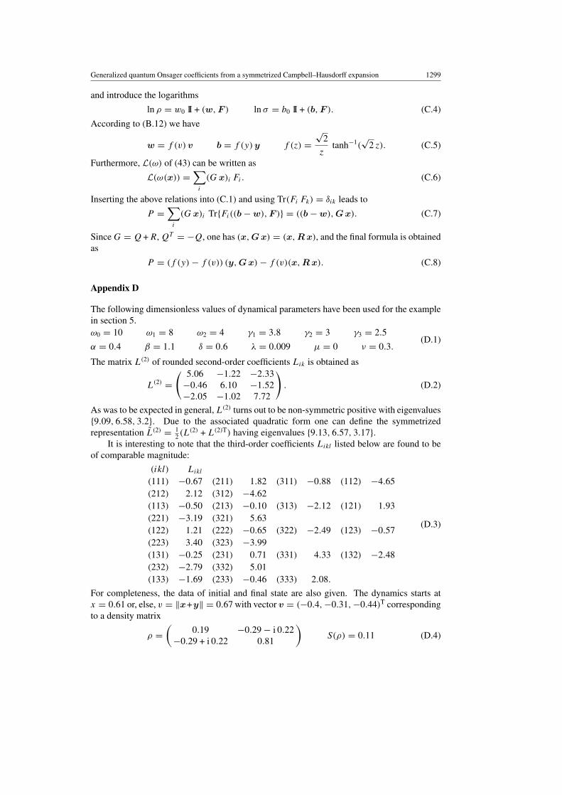
P = (f (y) − f (v)) (y,G x) − f (v)(x,R x). (C.8)

Appendix D

The following dimensionless values of dynamical parameters have been used for the examplein section 5.ω0 = 10 ω1 = 8 ω2 = 4 γ1 = 3.8 γ2 = 3 γ3 = 2.5

α = 0.4 β = 1.1 δ = 0.6 λ = 0.009 µ = 0 ν = 0.3.(D.1)

The matrix L(2) of rounded second-order coefficients Lik is obtained as

L(2) =( 5.06 −1.22 −2.33

−0.46 6.10 −1.52−2.05 −1.02 7.72

). (D.2)

As was to be expected in general, L(2) turns out to be non-symmetric positive with eigenvalues{9.09, 6.58, 3.2}. Due to the associated quadratic form one can define the symmetrizedrepresentation L(2) = 1

2 (L(2) + L(2)T) having eigenvalues {9.13, 6.57, 3.17}.

It is interesting to note that the third-order coefficients Likl listed below are found to beof comparable magnitude:

(ikl) Likl

(111) −0.67 (211) 1.82 (311) −0.88 (112) −4.65(212) 2.12 (312) −4.62(113) −0.50 (213) −0.10 (313) −2.12 (121) 1.93(221) −3.19 (321) 5.63(122) 1.21 (222) −0.65 (322) −2.49 (123) −0.57(223) 3.40 (323) −3.99(131) −0.25 (231) 0.71 (331) 4.33 (132) −2.48(232) −2.79 (332) 5.01(133) −1.69 (233) −0.46 (333) 2.08.

(D.3)

For completeness, the data of initial and final state are also given. The dynamics starts atx = 0.61 or, else, v = ‖x+y‖ = 0.67 with vector v = (−0.4,−0.31,−0.44)T correspondingto a density matrix

ρ =(

0.19 −0.29 − i 0.22−0.29 + i 0.22 0.81

)S(ρ) = 0.11 (D.4)


where S(ρ) = − Tr(ρ ln ρ) is the von Neumann entropy with bounds 0 � S � ln 2 =0.69. The final destination state is reached at x = 0 or, else, y = 0.11 with vectory = (−0.05,−0.04,−0.09)T equivalent to

σ =(

0.43 −0.04 − i 0.03−0.04 + i 0.03 0.57

)S(σ) = 0.68. (D.5)

These data show that the dynamics starts not far from a pure state close to the surface ofthe Bloch sphere (radius = 0.71) and ends almost in the centre, which belongs to maximumentropy S = 0.69.

References

[1] Onsager L 1931 Phys. Rev. 37 405Onsager L 1931 Phys. Rev. 38 2265

[2] de Groot S R and Mazur P 1962 Non-Equilibrium Thermodynamics (Amsterdam: North-Holland)[3] Callen H B 1960 Thermodynamics (New York: Wiley)[4] Ruelle D 1996 J. Stat. Phys. 85 1[5] de Groot S R 1960 Thermodynamik Irreversibler Prozesse (Mannheim: Bibliographisches Institut)[6] Gabrielli D, Jona-Lasinio G and Landim C 1996 Phys. Rev. Lett. 77 1202[7] Landauer R 1975 Phys. Rev. A 12 636[8] Streater R F 1993 J. Phys. A: Math. Gen. 26 1553[9] Alicki R 1976 Rep. Math. Phys. 10 249

[10] Alicki R 1979 J. Stat. Phys. 20 671[11] Alicki R 1979 J. Phys. A: Math. Gen. 12 L103[12] Spohn H 1978 J. Math. Phys. 19 1227[13] Spohn H and Lebowitz J L 1978 Advances in Chemical Physics vol 38, ed S A Rice (New York: Wiley)[14] Lendi K 1986 Phys. Rev. A 34 662[15] Alicki R and Lendi K 1987 Quantum Dynamical Semigroups and Applications (Lecture Notes in Physics vol 286)

(Berlin: Springer)[16] Lendi K 2000 J. Stat. Phys. 99 1037[17] Haake F 1973 Springer Tracts in Modern Physics vol 66, ed G Hohler (Berlin: Springer)[18] van Wonderen A J and Lendi K 1995 J. Stat. Phys. 80 273[19] Lendi K, Farhadmotamed F and van Wonderen A J 1998 J. Stat. Phys. 92 1115[20] Farhadmotamed F, van Wonderen A J and Lendi K 1998 J. Phys. A: Math. Gen. 31 3395[21] Farhadmotamed F 1998 Thesis University of Zurich[22] Gorini V, Kossakowski A and Sudarshan E C G 1976 J. Math. Phys. 17 821[23] Davies E B 1974 Commun. Math. Phys. 39 91

Davies E B 1976 Math. Ann. 219 147Davies E B 1975 Ann. Inst. Henri Poincare 11 265

[24] Ohya M and Petz D 1993 Quantum Entropy and its Use (Berlin: Springer)[25] Wehrl A 1978 Rev. Mod. Phys. 50 221[26] Thirring W 1980 Lehrbuch der Theoretischen Physik vol 4 (Vienna: Springer)[27] Lindblad G 1975 Commun. Math. Phys. 40 147[28] Magnus W 1954 Commun. Pure Appl. Math. 7 649[29] Weiss G H and Maradudin A A 1962 J. Math. Phys. 3 771[30] Lendi K 1987 J. Phys. A: Math. Gen. 20 15[31] Dufty J W and Rubi J M 1987 Phys. Rev. A 36 222[32] Abragam A 1986 Principles of Nuclear Magnetism (Oxford: Oxford University Press)[33] Slichter C P 1973 Priciples of Magnetic Resonance (Berlin: Springer)[34] Allen L and Eberly J H 1975 Optical Resonance and Two-Level Atoms (New York: Wiley)[35] Louisell W H 1973 Quantum Statistical Properties of Radiation (New York: Wiley)[36] Loudon R 1978 The Quantum Theory of Light (Oxford: Oxford University Press)[37] Dwight H B 1961 Tables of Integrals and other Mathematical Data (New York: Macmillan)[38] Hilgert J, Hofmann K H and Lawson J D 1989 Lie Groups, Convex Cones, and Semigroups (Oxford: Clarendon)[39] Bourbaki N 1989 Lie Groups and Lie Algebras (Berlin: Springer)[40] Oteo J A 1991 J. Math. Phys. 32 419

generalized quantum onsager coefficients from a symmetrized campbell-hausdorff expansion

Documents