generalized symmetric admm for separable convex …hozhang/papers/gs-admm.pdf · generalized...

Comput Optim Applhttps://doi.org/10.1007/s10589-017-9971-0

Generalized symmetric ADMM for separable convexoptimization

Jianchao Bai1 · Jicheng Li1 · Fengmin Xu2 ·Hongchao Zhang3

Received: 25 April 2017© Springer Science+Business Media, LLC, part of Springer Nature 2017

Abstract Thealternatingdirectionmethodofmultipliers (ADMM)has beenproved tobe effective for solving separable convex optimization subject to linear constraints. Inthis paper, we propose a generalized symmetric ADMM (GS-ADMM), which updatesthe Lagrange multiplier twice with suitable stepsizes, to solve the multi-block separa-ble convex programming. This GS-ADMMpartitions the data into two group variablesso that one group consists of p block variables while the other has q block variables,where p ≥ 1 and q ≥ 1 are two integers. The two grouped variables are updatedin a Gauss–Seidel scheme, while the variables within each group are updated in aJacobi scheme, which would make it very attractive for a big data setting. By addingproper proximal terms to the subproblems, we specify the domain of the stepsizes to

The work was supported by the National Science Foundation of China under Grants 11671318 and11571178, the Science Foundation of Fujian province of China under Grant 2016J01028, and the NationalScience Foundation of USA under Grant 1522654.

B Hongchao [email protected]

Jianchao [email protected]

Jicheng [email protected]

Fengmin [email protected]

1 School of Mathematics and Statistics, Xi’an Jiaotong University, Xi’an 710049,People’s Republic of China

2 School of Economics and Finance, Xi’an Jiaotong University, Xi’an 710049,People’s Republic of China

3 Department of Mathematics, Louisiana State University, Baton Rouge, LA 70803-4918, USA

123

http://crossmark.crossref.org/dialog/?doi=10.1007/s10589-017-9971-0&domain=pdf

J. Bai et al.

guarantee that GS-ADMM is globally convergent with a worst-case O(1/t) ergodicconvergence rate. It turns out that our convergence domain of the stepsizes is signifi-cantly larger than other convergence domains in the literature. Hence, the GS-ADMMis more flexible and attractive on choosing and using larger stepsizes of the dual vari-able. Besides, two special cases ofGS-ADMM,which allows using zero penalty terms,are also discussed and analyzed. Compared with several state-of-the-art methods, pre-liminary numerical experiments on solving a sparse matrix minimization problem inthe statistical learning show that our proposed method is effective and promising.

Keywords Separable convex programming ·Multiple blocks ·Parameter convergencedomain · Alternating direction method of multipliers · Global convergence ·Complexity · Statistical learning

Mathematics Subject Classification 65C60 · 65E05 · 68W40 · 90C06

1 Introduction

We consider the following grouped multi-block separable convex programming prob-lem

minp∑

i=1fi (xi ) +

q∑

j=1g j (y j )

s.t.p∑

i=1Ai xi +

q∑

j=1B j y j = c,

xi ∈ Xi , i = 1, . . . , p,

y j ∈ Y j , j = 1, . . . , q,

(1)

where fi (xi ) : Rmi → R, g j (y j ) : Rd j → R are closed and proper convex functions(possibly nonsmooth); Ai ∈ Rn×mi , B j ∈ Rn×d j and c ∈ Rn are given matrices andvectors, respectively; Xi ⊂ Rmi and Y j ⊂ Rd j are closed convex sets; p ≥ 1 andq ≥ 1 are two integers. Throughout this paper, we assume that the solution set of theproblem (1) is nonempty and all the matrices Ai , i = 1, . . . , p, and B j , j = 1, . . . , q,have full column rank. And in the following, we denote A = (

A1, . . . , Ap),B =

(B1, . . . , Bq

), x = (xT1 , . . . , xTp )T, y = (yT1 , . . . , yTq )T, X = X1 × X2 × · · ·Xp,

Y = Y1 × Y2 × · · ·Yq and M = X × Y × Rn .In the last few years, the problem (1) has been extensively investigated due to its

wide applications in different fields, such as the sparse inverse covariance estimationproblem [21] in finance and statistics, the model updating problem [4] in the designof vibration structural dynamic system and bridges, the low rank and sparse represen-tations [19] in image processing and so forth. One standard way to solve the problem(1) is the classical Augmented Lagrangian Method (ALM) [10], which minimizes thefollowing augmented Lagrangian function

Lβ (x, y, λ) = L (x, y, λ) + β

2‖Ax + By − c‖2,

123

Generalized symmetric ADMM for separable convex…

where β > 0 is a penalty parameter for the equality constraint and

L (x, y, λ) =p∑

i=1

fi (xi ) +q∑

j=1

g j (y j ) − 〈λ,Ax + By − c〉 (2)

is the Lagrangian function of the problem (1) with the Lagrange multiplier λ ∈ Rn .Then, the ALM procedure for solving (1) can be described as follows:

{(xk+1, yk+1

) = argmin{Lβ

(x, y, λk

) | x ∈ X , y ∈ Y},

λk+1 = λk − β(Axk+1 + Byk+1 − c).

However, ALM does not make full use of the separable structure of the objectivefunction of (1) and hence, could not take advantage of the special properties of thecomponent objective functions fi and g j in (1). As a result, in many recent real appli-cations involving big data, solving the subproblems of ALM becomes very expensive.

One effective approach to overcome such difficulty is the Alternating DirectionMethod of Multipliers (ADMM), which was originally proposed in [8] and could beregarded as a splitting version of ALM. At each iteration, ADMM first sequentiallyoptimize over one block variable while fixing all the other block variables, and thenfollows byupdating theLagrangemultiplier.Anatural extension ofADMMfor solvingthe multi-block case problem (1) takes the following iterations:

⎧⎪⎪⎪⎪⎪⎪⎪⎨

⎪⎪⎪⎪⎪⎪⎪⎩

For i = 1, 2, . . . , p,

xk+1i = arg min

xi ∈Xi

Lβ

(xk+11 , . . . , xk+1

i−1 , xi , xki+1, . . . , xk

p, yk, λk

),

For j = 1, 2, . . . , q,

yk+1j = arg min

y j ∈Y j

Lβ

(xk+1, yk+1

1 , . . . , yk+1j−1, y j , yk

j+1, . . . , ykq , λk

),

λk+1 = λk − β(Axk+1 + Byk+1 − c

).

(3)

Obviously, the scheme (3) is a serial algorithmwhich uses the newest information of thevariables at each iteration. Although the above scheme was proved to be convergentfor the two-block, i.e., p = q = 1, separable convex minimization (see [11]), asshown in [3], the direct extension of ADMM (3) for the multi-block case, i.e., p +q ≥ 3, without proper modifications is not necessarily convergent. Another naturalextension of ADMM is to use the Jacobian fashion, where the variables are updatedsimultaneously after each iteration, that is,

⎧⎪⎪⎪⎪⎪⎪⎪⎨

⎪⎪⎪⎪⎪⎪⎪⎩

For i = 1, 2, . . . , p,

xk+1i = arg min

xi ∈Xi

Lβ

(xk1 , . . . , xk

i−1, xi , xki+1, . . . , xk

p, yk, λk

),

For j = 1, 2, . . . , q,

yk+1j = arg min

y j ∈Y j

Lβ

(xk, yk

1 , . . . , ykj−1, y j , yk

j+1, . . . , ykq , λk

),

λk+1 = λk − β(Axk+1 + Byk+1 − c

).

(4)

As shown in [13], however, the Jacobian scheme (4) is not necessarily convergenteither. To ensure the convergence,He et al. [14] proposed a novelADMM-type splitting

123

J. Bai et al.

method that by adding certain proximal terms, allowed some of the subproblems to besolved in parallel, i.e., in a Jacobian fashion. And in [14], some sparse low-rankmodelsand image painting problems were tested to verify the efficiency of their method.

More recently, a Symmetric ADMM (S-ADMM)was proposed by He et al. [16] forsolving the two-block separable convex minimization, where the algorithm performsthe following updating scheme:

⎧⎪⎪⎪⎪⎨

⎪⎪⎪⎪⎩

xk+1 = argmin{Lβ

(x, yk, λk

) | x ∈ X },

λk+ 12 = λk − τβ

(Axk+1 + Byk − c),

yk+1 = argmin{Lβ(xk+1, y, λk+ 1

2 ) | y ∈ Y}

,

λk+1 = λk+ 12 − sβ

(Axk+1 + Byk+1 − c),

(5)

and the stepsizes (τ, s) were restricted into the domain

H ={(τ, s) | s ∈ (0, (

√5 + 1)/2), τ + s > 0, τ ∈ (−1, 1), |τ | < 1 + s − s2

}

(6)in order to ensure its global convergence. The main improvement of [16] is that thescheme (5) largely extends the domain of the stepsizes (τ, s) of other ADMM-typemethods [12]. What’s more, the numerical performance of S-ADMM on solving thewidely used basis pursuit model and the total-variational image debarring model sig-nificantly outperforms the original ADMM in both the CPU time and the number ofiterations. Besides, Gu, et al.[9] also studied a semi-proximal-based strictly contrac-tive Peaceman-Rachford splitting method, that is (5) with two additional proximalpenalty terms for the x and y update. But their method has a nonsymmetric conver-gence domain of the stepsize and still focuses on the two-block case problem, whichlimits its applications for solving large-scale problems with multiple block variables.

Mainly motivated by the work of [9,14,16], we would like to generalize S-ADMMwith more wider convergence domain of the stepsizes to tackle the multi-block sep-arable convex programming model (1), which more frequently appears in recentapplications involving big data [2,20]. Our algorithm framework can be describedas follows:

(GS-ADMM)

⎧⎪⎪⎪⎪⎪⎪⎪⎪⎪⎪⎪⎪⎪⎪⎪⎨

⎪⎪⎪⎪⎪⎪⎪⎪⎪⎪⎪⎪⎪⎪⎪⎩

For i = 1, 2, . . . , p,

xk+1i = arg min

xi ∈Xi

Lβ(xk1 , . . . , xi , . . . , xk

p, yk, λk) + Pk

i (xi ),

where Pki (xi ) = σ1β

2

∥∥Ai (xi − xk

i )∥∥2 ,

λk+ 12 = λk − τβ(Axk+1 + Byk − c),

For j = 1, 2, . . . , q,

yk+1j = arg min

y j ∈Y j

Lβ(xk+1, yk1 , . . . , y j , . . . , yk

q , λk+ 12 ) + Qk

j (y j ),

where Qkj (y j ) = σ2β

2

∥∥∥B j (y j − yk

j )

∥∥∥2,

λk+1 = λk+ 12 − sβ(Axk+1 + Byk+1 − c).

(7)

123


Fig. 1 Stepsize region K of GS-ADMM

In the above generalized symmetric ADMM (GS-ADMM), τ and s are two stepsizeparameters satisfying

(τ, s) ∈ K ={(τ, s) | τ + s > 0, τ ≤ 1, −τ 2 − s2 − τ s + τ + s + 1 > 0

}, (8)

and σ1 ∈ (p − 1,+∞), σ2 ∈ (q − 1,+∞) are two proximal parameters1 for theregularization terms Pk

i (·) and Qkj (·). He and Yuan[15] also investigated the above

GS-ADMM (7) but restricted the stepsize τ = s ∈ (0, 1), which does not exploit theadvantages of using flexible stepsizes given in (8) to improve its convergence.

Major contributions of this paper can be summarized as the following four aspects:

– Firstly, the new GS-ADMM could deal with the multi-block separable convexprogramming problem (1), while the original S-ADMM in [16] only works forthe two block case and may not be convenient for solving large-scale problems. Inaddition, the convergence domainK for the stepsizes (τ, s) in (8), shown in Fig. 1,is significantly larger than the domainH given in (6) and the convergence domainin [9,15]. For example, the stepsize s can be arbitrarily close to 5/3 when thestepsize τ is close to −1/3. Moreover, the above domain in (8) is later enlarged toa symmetric domain G defined in (73), shown in Fig. 2. Numerical experiments inSec. 5.2.1 also validate that usingmore flexible and relatively larger stepsizes (τ, s)can often improve the convergence speed ofGS-ADMM.On the other hand,we cansee that when τ = 0, the stepsize s can be chosen in the interval (0, (

√5+ 1)/2),

which was firstly suggested by Fortin and Glowinski in [5,7].

1 Note that these two parameters are strictly positive in (7). In Sect. 4, however, we analyze two specialcases of GS-ADMM allowing either σ1 or σ2 to be zero.

123

J. Bai et al.

Fig. 2 Stepsize region G of GS-ADMM

– Secondly, the global convergence of GS-ADMM as well as its worst-caseO(1/t)ergodic convergence rate are established. What’s more, the total p + q blockvariables are partitioned into two grouped variables.While aGauss–Seidel fashionis taken between the two grouped variables, the block variables within each groupare updated in a Jacobi scheme. Hence, parallel computing can be implemented forupdating the variables within each group, which could be critical in some scenariosfor problems involving big data.

– Thirdly, we discuss two special cases of GS-ADMM,which is (7) with p ≥ 1, q =1 and σ2 = 0 or with p = 1, q ≥ 1 and σ1 = 0. These two special cases of GS-ADMM were not discussed in [15] and in fact, to the best of our knowledge, theyhave not been studied in the literature. We show the convergence domain of thestepsizes (τ, s) for these two cases is still K defined in (8) that is larger thanH.

– Finally, numerical experiments are performed on solving a sparse matrix opti-mization problem arising from the statistical learning. We have investigated theeffects of the stepsizes (τ, s) and the penal parameter β on the performance of GS-ADMM. And our numerical experiments demonstrate that by properly choosingthe parameters, GS-ADMM could perform significantly better than other recentlyquite popular methods developed in [1,14,17,23].

The paper is organized as follows. In Sect. 2, some preliminaries are given to refor-mulate the problem (1) into a variational inequality and to interpret the GS-ADMM(7) as a prediction–correction procedure. Section 3 investigates some properties of‖wk − w∗‖2H and provides a lower bound of ‖wk − wk‖2G , where H and G aresome particular symmetric matrices. Then, we establish the global convergence ofGS-ADMM and show its convergence rate in an ergodic sense. In Sect. 4, we discusstwo special cases of GS-ADMM, in which either the penalty parameters σ1 or σ2 is

123


allowed to be zero. Some preliminary numerical experiments are done in Sect. 5. Wefinally make some conclusions in Sect. 6.

1.1 Notation

Denoted by R,Rn,Rm×n be the set of real numbers, the set of n dimensional realcolumn vectors and the set of m × n real matrices, respectively. For any x, y ∈ Rn ,〈x, y〉 = xTy denotes their inner product and ‖x‖ = √〈x, x〉 denotes the Euclideannorm of x , where the superscript T is the transpose. Given a symmetric matrix G,we define ‖x‖2G = xTGx . Note that with this convention, ‖x‖2G is not necessarilynonnegative unless G is a positive definite matrix ( 0). For convenience, we use Iand 0 to stand respectively for the identity matrix and the zero matrix with properdimension throughout the context.

2 Preliminaries

In this section, we first use a variational inequality to characterize the solution set ofthe problem (1). Then, we analyze that GS-ADMM (7) can be treated as a prediction–correction procedure involving a prediction step and a correction step.

2.1 Variational reformulation of (1)

We begin with the following standard lemma whose proof can be found in [16,18].

Lemma 1 Let f : Rm −→ R and h : Rm −→ R be two convex functions definedon a closed convex set Ω ⊂ Rm and h is differentiable. Suppose that the solution setΩ∗ = argmin

x∈Ω{ f (x) + h(x)} is nonempty. Then, we have

x∗ ∈ Ω∗ if and only if x∗ ∈ Ω, f (x) − f (x∗) + ⟨x − x∗,∇h(x∗)

⟩ ≥ 0,∀x ∈ Ω.

It is well-known in optimization that a triple point (x∗, y∗, λ∗) ∈ M is called thesaddle-point of the Lagrangian function (2) if it satisfies

L(x∗, y∗, λ

) ≤ L(x∗, y∗, λ∗) ≤ L

(x, y, λ∗) , ∀(x, y, λ) ∈ M

which can be also characterized as

⎧⎪⎪⎪⎪⎪⎪⎪⎪⎨

⎪⎪⎪⎪⎪⎪⎪⎪⎩

For i = 1, 2, . . . , p,

x∗i = arg min

xi ∈Xi

Lβ

(x∗1 , . . . , x∗

i−1, xi , x∗i+1, . . . , x∗

p, y∗, λ∗

),

For j = 1, 2, . . . , q,

y∗j = arg min

y j ∈Y j

Lβ

(x∗, y∗

1 , . . . , y∗j−1, y j , y∗

j+1, . . . , y∗q , λ∗

),

λ∗ = arg maxλ∈Rn

Lβ (x∗, y∗, λ) .

123

J. Bai et al.

Then, by Lemma 1, the above saddle-point equations can be equivalently expressedas

⎧⎪⎪⎪⎪⎨

⎪⎪⎪⎪⎩

For i = 1, 2, . . . , p,

x∗i ∈ Xi , fi (xi ) − fi (x∗

i ) + 〈xi − x∗i ,−AT

i λ∗〉 ≥ 0,∀xi ∈ Xi ,

For j = 1, 2, . . . , q,

y∗j ∈ Y j , g j (y j ) − g j (y∗

j ) + 〈y j − y∗j ,−BT

j λ∗〉 ≥ 0,∀y j ∈ Y j ,

λ∗ ∈ Rn, 〈λ − λ∗,Ax∗ + By∗ − c〉 ≥ 0,∀λ ∈ Rn .

(9)

Rewriting (9) in a more compact variational inequality (VI) form, we have

h(u) − h(u∗) + ⟨w − w∗,J (w∗)

⟩ ≥ 0, ∀w ∈ M, (10)

where

h(u) =p∑

i=1

fi (xi ) +p∑

j=1

g j (y j )

and

u =(xy

)

, w =⎛

⎝xyλ

⎞

⎠ , J (w) =⎛

⎝−ATλ

−BTλ

Ax + By − c

⎞

⎠ .

Noticing that the affine mapping J is skew-symmetric, we immediately get

〈w − w,J (w) − J (w)〉 = 0, ∀ w, w ∈ M. (11)

Hence, (10) can be also rewritten as

VI(h,J ,M) : h(u) − h(u∗) + ⟨w − w∗,J (w)

⟩ ≥ 0, ∀w ∈ M. (12)

Because of the nonempty assumption on the solution set of (1), the solution setM∗ of the variational inequality VI(h,J ,M) is also nonempty and convex, see e.g.Theorem 2.3.5 [6] for more details. The following theorem given by Theorem 2.1 [11]provides a concrete way to characterize the set M∗.

Theorem 1 The solution set of the variational inequality VI(h,J ,M) is convex andcan be expressed as

M∗ =⋂

w∈M{w ∈ M| h(u) − h(u) + 〈w − w,J (w)〉 ≥ 0} .

123


2.2 A prediction–correction interpretation of GS-ADMM

Following a similar approach in [16], we next interpret GS-ADMM as a prediction–correction procedure. First, let

xk =

⎛

⎜⎜⎜⎝

x k1

x k2...

x kp

⎞

⎟⎟⎟⎠

=

⎛

⎜⎜⎜⎝

xk+11

xk+12...

xk+1p

⎞

⎟⎟⎟⎠

, yk =

⎛

⎜⎜⎜⎝

yk1

yk2...

ykq

⎞

⎟⎟⎟⎠

=

⎛

⎜⎜⎜⎝

yk+11

yk+12...

yk+1q

⎞

⎟⎟⎟⎠

, (13)

λk = λk − β(Axk+1 + Byk − c

), (14)

and

u =(xy

)

, wk =⎛

⎝xk

yk

λk

⎞

⎠ =⎛

⎝xk+1

yk+1

λk

⎞

⎠ . (15)

Then, by using the above notations, we derive the following basic lemma.

Lemma 2 For the iterates uk, wk defined in (15), we have wk ∈ M and

h(u) − h(uk) +⟨w − wk,J (wk) + Q(wk − wk)

⟩≥ 0, ∀w ∈ M, (16)

where

Q =[

Hx 00 Q

]

(17)

with

Hx = β

⎡

⎢⎢⎢⎢⎢⎢⎢⎢⎢⎣

σ1AT1 A1 −AT

1 A2 · · · −AT1 Ap

−AT2 A1 σ1AT

2 A2 · · · −AT2 Ap

......

. . ....

−ATp A1 −AT

p A2 · · · σ1ATp Ap

⎤

⎥⎥⎥⎥⎥⎥⎥⎥⎥⎦

, (18)

Q =

⎡

⎢⎢⎢⎢⎢⎢⎢⎢⎢⎢⎢⎢⎢⎢⎣

(σ2 + 1)βBT1 B1 0 · · · 0 −τ BT

1

0 (σ2 + 1)βBT2 B2 · · · 0 −τ BT

2

......

. . ....

...

0 0 · · · (σ2 + 1)βBTq Bq −τ BT

q

−B1 −B2 · · · −Bq1β

I

⎤

⎥⎥⎥⎥⎥⎥⎥⎥⎥⎥⎥⎥⎥⎥⎦

.

(19)

123

J. Bai et al.

Proof Omitting some constants, it is easy to verify that the xi -subproblem (i =1, 2, . . . , p) of GS-ADMM can be written as

xk+1i = arg min

xi ∈Xi

{

fi (xi )− 〈λk, Ai xi 〉 + β

2

∥∥Ai xi − cx,i

∥∥2 + σ1β

2

∥∥∥Ai (xi − xk

i )

∥∥∥2}

,

where cx,i = c −p∑

l=1,l �=iAl xk

l − Byk . Hence, by Lemma 1, we have xk+1i ∈ Xi and

fi (xi ) − fi (xk+1i ) +

⟨Ai (xi − xk+1

i ),−λk + β(Ai xk+1i − cx,i )

+ σ1β Ai (xk+1i − xk

i )⟩≥ 0

for any xi ∈ Xi . So, by the definition of (13) and (14), we get

fi (xi ) − fi (xki ) +

⟨

Ai (xi − x ki ), −λk − β

p∑

l=1,l �=i

Al (xkl − xk

l )

+ σ1β

p∑

l=1

Al (xkl − xk

l )

⟩

≥ 0 (20)

for any xi ∈ Xi . By the way of generating λk+ 12 in (7) and the definition of (14), the

following relation holds

λk+ 12 = λk − τ(λk − λk ). (21)

Similarly, the y j -subproblem ( j = 1, . . . , q) of GS-ADMM can be written as

yk+1j = arg min

y j ∈Y j

{

g j (y j )−⟨λk+ 1

2 , B j y j

⟩+ β

2

∥∥B j y j − cy, j

∥∥2 + σ2β

2

∥∥∥B j (y j − yk

j )∥∥∥2}

,

where cy, j = c − Axk+1 −q∑

l=1,l �= jBl yk

l . Hence, by Lemma 1, we have yk+1j ∈ Y j

and

g j (y j ) − g j (yk+1j ) +

⟨B j (y j − yk+1

j ),−λk+ 12 + β(B j yk+1

j − cy, j )

+ σ2βB j (yk+1j − yk

j )⟩≥ 0

for any y j ∈ Y j . This inequality, by using (21) and the definition of (13) and (14), canbe rewritten as

g j (y j ) − g j (ykj ) +

⟨B j (y j − yk

j ), −λk + (σ2 + 1)βB j (ykj − yk

j ) − τ (λk − λk)⟩≥ 0

(22)

123


for any y j ∈ Y j . Besides, the equality (14) can be rewritten as

(Axk + Byk − c

)− B

(yk − yk

)+ 1

β(λk − λk) = 0,

which is equivalent to

⟨

λ − λk, (Axk + Byk − c) − B(yk − yk) + 1

β(λk − λk)

⟩

≥ 0, ∀λ ∈ Rn . (23)

Then, (16) follows from (20), (22) and (23). ��Lemma 3 For the sequences {wk} and {wk} generated by GS-ADMM, the followingequality holds

wk+1 = wk − M(wk − wk), (24)

where

M =

⎡

⎢⎢⎢⎢⎢⎣

II

. . .

I−sβB1 · · · −sβBq (τ + s)I

⎤

⎥⎥⎥⎥⎥⎦

. (25)

Proof It follows from the way of generating λk+1 in the algorithm and (21) that

λk+1 = λk+ 12 − sβ(Axk+1 + Byk+1 − c)

= λk+ 12 − sβ(Axk+1 + Byk − c) + sβB(yk − yk+1)

= λk − τ(λk − λk) − s(λk − λk) + sβB(yk − yk)

= λk − [−sβB(yk − yk) + (τ + s)(λk − λk)].

The above equality together with xk+1i = x k

l , for i = 1, . . . , p, and yk+1j = yk

j , forj = 1, . . . , q, imply

⎛

⎜⎜⎜⎜⎜⎜⎜⎜⎜⎜⎜⎜⎜⎝

xk+11

.

.

.

xk+1p

yk+11

.

.

.

yk+1q

λk+1

⎞

⎟⎟⎟⎟⎟⎟⎟⎟⎟⎟⎟⎟⎟⎠

=

⎛

⎜⎜⎜⎜⎜⎜⎜⎜⎜⎜⎜⎜⎝

xk1

.

.

.

xkp

yk1

.

.

.

ykq

λk

⎞

⎟⎟⎟⎟⎟⎟⎟⎟⎟⎟⎟⎟⎠

−

⎡

⎢⎢⎢⎢⎢⎢⎢⎢⎢⎢⎢⎢⎢⎣

I

. . .

I

I

. . .

I

−sβB1 · · · −sβBq (τ + s)I

⎤

⎥⎥⎥⎥⎥⎥⎥⎥⎥⎥⎥⎥⎥⎦

⎛

⎜⎜⎜⎜⎜⎜⎜⎜⎜⎜⎜⎜⎝

xk1 − xk

1

.

.

.

xkp − xk

p

yk1 − yk

1

.

.

.

ykq − yk

q

λk − λk

⎞

⎟⎟⎟⎟⎟⎟⎟⎟⎟⎟⎟⎟⎠

,

which immediately gives (24). ��

123

J. Bai et al.

Lemmas 2 and 3 show that our GS-ADMM can be interpreted as a prediction–correction framework, where wk+1 and wk are normally called the predictive variableand the correcting variable, respectively.

3 Convergence analysis of GS-ADMM

Compared with (12) and (16), the key for proving the convergence of GS-ADMM isto verify that the extra term in (16) converges to zero, that is,

limk→∞

⟨w − wk, Q(wk − wk)

⟩= 0, ∀w ∈ M.

In this section, we first investigate some properties of the sequence {‖wk − w∗‖2H }.Then, we provide a lower bound of ‖wk − wk‖2G . Based on these properties, the globalconvergence and worst-case O(1/t) convergence rate of GS-ADMM are establishedin the end.

3.1 Properties of{∥∥wk − w∗∥∥2

H

}

It follows from (11) and (16) that wk ∈ M and

h(u) − h(uk) +⟨w − wk,J (w)

⟩≥


⟩, ∀w ∈ M. (26)

Suppose τ + s > 0. Then, the matrix M defined in (25) is nonsingular. So, by (24)and a direct calculation, the right-hand term of (26) is rewritten as


⟩=

⟨w − wk, H(wk − wk+1)

⟩(27)

where

H = QM−1 =[

Hx 0

0 H

]

(28)

with Hx defined in (18) and

H =

⎡

⎢⎢⎢⎢⎢⎢⎢⎢⎢⎢⎣

(σ2 + 1 − τ sτ+s )βBT

1 B1 · · · − τ sτ+s βBT

1 Bq − ττ+s BT

1

.... . .

......

− τ sτ+s βBT

q B1 · · · (σ2 + 1 − τ sτ+s )βBT

q Bq − ττ+s BT

q

− ττ+s B1 · · · − τ

τ+s Bq1

β(τ+s) I

⎤

⎥⎥⎥⎥⎥⎥⎥⎥⎥⎥⎦

.

(29)The following lemma shows that H is a positive definite matrix for proper choice

of the parameters (σ1, σ2, τ, s).

123


Lemma 4 The matrix H defined in (28) is symmetric positive definite if

σ1 ∈ (p − 1,+∞), σ2 ∈ (q − 1,+∞), τ ≤ 1 and τ + s > 0. (30)

Proof By the block structure of H , we only need to show that the blocks Hx and Hin (28) are positive definite if the parameters (σ1, σ2, τ, s) satisfy (30). Note that

Hx = β

⎡

⎢⎢⎢⎣

A1A2

. . .

Ap

⎤

⎥⎥⎥⎦

T

Hx,0

⎡

⎢⎢⎢⎣

A1A2

. . .

Ap

⎤

⎥⎥⎥⎦

, (31)

where

Hx,0 =

⎡

⎢⎢⎢⎣

σ1 I −I · · · −I−I σ1 I · · · −I...

.... . .

...

−I −I · · · σ1 I

⎤

⎥⎥⎥⎦

p×p

. (32)

If σ1 ∈ (p − 1,+∞), Hx,0 is positive definite. Then, it follows from (31) that Hx ispositive definite if σ1 ∈ (p −1,+∞) and all Ai , i = 1, . . . , p, have full column rank.

Now, note that the matrix H can be decomposed as

H = DT H0 D, (33)

where

D =

⎡

⎢⎢⎢⎢⎢⎢⎢⎣

β12 B1

β12 B2

. . .

β12 Bq

β− 12 I

⎤

⎥⎥⎥⎥⎥⎥⎥⎦

(34)

and

H0 =

⎡

⎢⎢⎢⎢⎢⎢⎢⎢⎢⎢⎢⎢⎢⎢⎢⎢⎢⎣

(σ2 + 1 − τ s

τ+s

)I − τ s

τ+s I · · · − τ sτ+s I − τ

τ+s I

− τ sτ+s I

(σ2 + 1 − τ s

τ+s

)I · · · − τ s

τ+s I − ττ+s I

......

. . ....

...

− τ sτ+s I − τ s

τ+s I · · ·(σ2 + 1 − τ s

τ+s

)I − τ

τ+s I

− ττ+s I − τ

τ+s I · · · − ττ+s I 1

τ+s I

⎤

⎥⎥⎥⎥⎥⎥⎥⎥⎥⎥⎥⎥⎥⎥⎥⎥⎥⎦

.

123

J. Bai et al.

According to the fact that

⎡

⎢⎣

I τ I. . . τ I

I

⎤

⎥⎦ H0

⎡

⎢⎣

I τ I. . . τ I

I

⎤

⎥⎦

T

=

⎡

⎢⎢⎢⎢⎢⎢⎢⎢⎢⎢⎢⎢⎢⎣

(σ2 + 1 − τ)I −τ I · · · −τ I 0

−τ I (σ2 + 1 − τ)I · · · −τ I 0

......

. . ....

...

−τ I −τ I · · · (σ2 + 1 − τ)I 0

0 0 · · · 0 1τ+s I

⎤

⎥⎥⎥⎥⎥⎥⎥⎥⎥⎥⎥⎥⎥⎦

=⎡

⎣Hy,0 + (1 − τ)E ET 0

0 1τ+s I

⎤

⎦ ,

where

E =

⎡

⎢⎢⎢⎣

II...

I

⎤

⎥⎥⎥⎦

and Hy,0 =

⎡

⎢⎢⎢⎣

σ2 I −I · · · −I−I σ2 I · · · −I...

.... . .

...

−I −I · · · σ2 I

⎤

⎥⎥⎥⎦

q×q

, (35)

we have H0 is positive definite if and only if Hy,0+(1−τ)E ET is positive definite andτ + s > 0. Note that Hy,0 is positive definite if σ2 ∈ (q − 1,+∞), and (1 − τ)E ET

is positive semidefinite if τ ≤ 1. So, H0 is positive definite if σ2 ∈ (q − 1,+∞),τ ≤ 1 and τ + s > 0. Then, it follows from (33) that H is positive definite, ifσ2 ∈ (q − 1,+∞), τ ≤ 1, τ + s > 0 and all the matrices B j , j = 1, . . . , q, have fullcolumn rank.

Summarizing the above discussions, the matrix H is positive definite if the param-eters (σ1, σ2, τ, s) satisfy (30). ��Theorem 2 The sequences {wk} and {wk} generated by GS-ADMM satisfy

h(u) − h(uk) +⟨w − wk,J (w)

⟩≥ 1

2

{∥∥∥w − wk+1

∥∥∥2

H−

∥∥∥w − wk

∥∥∥2

H

}

+1

2

∥∥∥wk − wk

∥∥∥2

G, ∀w ∈ M, (36)

whereG = Q + QT − MTH M. (37)

123


Proof By substituting

a = w, b = wk, c = wk, d = wk+1,

into the following identity

2〈a − b, H(c − d)〉 = ‖a − d‖2H − ‖a − c‖2H + ‖c − b‖2H − ‖d − b‖2H ,

we have

2⟨w − wk, H(wk − wk+1)

⟩

=∥∥∥w − wk+1

∥∥∥2

H−

∥∥∥w − wk

∥∥∥2

H+

∥∥∥wk − wk

∥∥∥2

H−

∥∥∥wk+1 − wk

∥∥∥2

H. (38)

Now, notice that

∥∥∥wk − wk

∥∥∥2

H−

∥∥∥wk+1 − wk

∥∥∥2

H

=∥∥∥wk − wk

∥∥∥2

H−

∥∥∥wk − wk + wk − wk+1

∥∥∥2

H

=∥∥∥wk − wk

∥∥∥2

H−

∥∥∥wk − wk + M(wk − wk)

∥∥∥2

H

=⟨wk − wk,

(H M + (H M)T − MTH M

)(wk − wk)

⟩

=⟨wk − wk,

(Q + QT − MTH M

)(wk − wk)

⟩, (39)

where the second equality holds by (24) and the fourth equality follows from (28).Then, (36) follows from (26)–(27), (38)–(39) and the definition of G in (37). ��Theorem 3 The sequences {wk} and {wk} generated by GS-ADMM satisfy

∥∥∥wk+1 − w∗

∥∥∥2

H≤

∥∥∥wk − w∗

∥∥∥2

H−

∥∥∥wk − wk

∥∥∥2

G, ∀w∗ ∈ M∗. (40)

Proof Setting w = w∗ ∈ M∗ in (36) we have

1

2

∥∥∥wk+1 − w∗

∥∥∥2

H≤ 1

2

∥∥∥wk − w∗

∥∥∥2

H− 1

2

∥∥∥wk − wk

∥∥∥2

G+ h(u∗) − h(uk)

+⟨w∗ − wk,J (w∗)

⟩.

The above inequality together with (10) reduces to the inequality (40). ��It can be observed that if

∥∥wk − wk

∥∥2

G is positive, then the inequality (40) impliesthe contractiveness of the sequence {wk −w∗} under the H -weighted norm. However,thematrixG defined in (37) is not necessarily positive definitewhenσ1 ∈ (p−1,+∞),σ2 ∈ (q − 1,+∞) and (τ, s) ∈ K. Therefore, it is necessary to estimate the lower

bound of∥∥wk − wk

∥∥2

G for the sake of the convergence analysis.

123

J. Bai et al.

3.2 Lower bound of∥∥wk − wk

∥∥2G

This subsection provides a lower bound of∥∥wk − wk

∥∥2

G , for σ1 ∈ (p − 1,+∞),σ2 ∈ (q − 1,+∞) and (τ, s) ∈ K, where K is defined in (8).

By simple calculations, the G given in (37) can be explicitly written as

G =[

Hx 0

0 G

]

,

where Hx is defined in (18) and

G =

⎡

⎢⎢⎢⎢⎢⎢⎢⎢⎢⎢⎣

(σ2 + 1 − s)βBT1 B1 · · · −sβBT

1 Bq (s − 1)BT1

.... . .

......

−sβBTq B1 · · · (σ2 + 1 − s)βBT

q Bq (s − 1)BTq

(s − 1)B1 · · · (s − 1)Bq2−τ−s

βI

⎤

⎥⎥⎥⎥⎥⎥⎥⎥⎥⎥⎦

. (41)

In addition, we have

G = DTG0 D,

where D is defined in (34) and

G0 =

⎡

⎢⎢⎢⎢⎢⎢⎢⎢⎢⎢⎢⎢⎢⎣

(σ2 + 1 − s)I −s I · · · −s I (s − 1)I

−s I (σ2 + 1 − s)I · · · −s I (s − 1)I

......

. . ....

...

−s I −s I · · · (σ2 + 1 − s)I (s − 1)I

(s − 1)I (s − 1)I · · · (s − 1)I (2 − τ − s)I

⎤

⎥⎥⎥⎥⎥⎥⎥⎥⎥⎥⎥⎥⎥⎦

.

(42)Now,wepresent the following lemmawhich provides a lower boundof ‖wk−wk‖G .

Lemma 5 Suppose σ1 ∈ (p − 1,+∞) and σ2 ∈ (q − 1,+∞). For the sequences{wk} and {wk} generated by GS-ADMM, there exists ξ1 > 0 such that

∥∥∥wk − wk

∥∥∥2

G≥ ξ1

⎛

⎝p∑

i=1

∥∥∥Ai

(xk

i − xk+1i

)∥∥∥2 +

q∑

j=1

∥∥∥B j

(yk

j − yk+1j

)∥∥∥2

⎞

⎠

123


+ (1 − τ)β

∥∥∥B

(yk − yk+1

)∥∥∥2

+ (2 − τ − s)β∥∥∥Axk+1 + Byk+1 − c

∥∥∥2

+ 2(1 − τ)β(Axk+1 + Byk+1 − c

)T B(yk − yk+1

). (43)

Proof First, it is easy to derive that

‖wk − wk‖2G =

∥∥∥∥∥∥∥∥∥∥∥∥∥∥∥∥∥∥∥∥

⎛

⎜⎜⎜⎜⎜⎜⎜⎜⎜⎜⎜⎜⎜⎜⎝

A1

(xk1 − xk+1

1

)

...

Ap

(xk

p − xk+1p

)

B1

(yk1 − yk+1

1

)

...

Bq

(yk

q − yk+1q

)

Axk+1 + Byk+1 − c

⎞

⎟⎟⎟⎟⎟⎟⎟⎟⎟⎟⎟⎟⎟⎟⎠

∥∥∥∥∥∥∥∥∥∥∥∥∥∥∥∥∥∥∥∥

2

G

,

where

G = β

⎡

⎢⎢⎢⎣

II I

. . ....

I

⎤

⎥⎥⎥⎦

[Hx,0

G0

]

⎡

⎢⎢⎢⎣

II I

. . ....

I

⎤

⎥⎥⎥⎦

T

= β

[Hx,0

G0

]

,

with Hx,0 and G0 defined in (32) and (42), respectively, and

G0 =

⎡

⎢⎢⎢⎢⎢⎢⎢⎢⎢⎢⎢⎢⎢⎣

(σ2 + 1 − τ)I −τ I · · · −τ I (1 − τ)I

−τ I (σ2 + 1 − τ)I · · · −τ I (1 − τ)I

......

. . ....

...

−τ I −τ I · · · (σ2 + 1 − τ)I (1 − τ)I

(1 − τ)I (1 − τ)I · · · (1 − τ)I (2 − τ − s)I

⎤

⎥⎥⎥⎥⎥⎥⎥⎥⎥⎥⎥⎥⎥⎦

=

⎡

⎢⎢⎢⎣

(1 − τ)I

Hy,0 + (1 − τ)E ET ...

(1 − τ)I(1 − τ)I · · · (1 − τ)I (2 − τ − s)I

⎤

⎥⎥⎥⎦

.

123

J. Bai et al.

In the above matrix G0, E and Hy,0 are defined in (35). Hence, we have

1

β

∥∥∥wk − wk

∥∥∥2

G=

∥∥∥∥∥∥∥∥∥∥∥∥

⎛

⎜⎜⎜⎜⎜⎜⎝

A1

(xk1 − xk+1

1

)

A2

(xk2 − xk+1

2

)

...

Ap

(xk

p − xk+1p

)

⎞

⎟⎟⎟⎟⎟⎟⎠

∥∥∥∥∥∥∥∥∥∥∥∥

2

Hx,0

+

∥∥∥∥∥∥∥∥∥∥∥∥

⎛

⎜⎜⎜⎜⎜⎜⎝

B1

(yk1 − yk+1

1

)

B2

(yk2 − yk+1

2

)

...

Bq

(yk

q − yk+1q

)

⎞

⎟⎟⎟⎟⎟⎟⎠

∥∥∥∥∥∥∥∥∥∥∥∥

2

Hy,0

+

∥∥∥∥∥∥∥∥∥∥∥∥

⎛

⎜⎜⎜⎜⎜⎜⎝

B1

(yk1 − yk+1

1

)

B2

(yk2 − yk+1

2

)

...

Bq

(yk

q − yk+1q

)

⎞

⎟⎟⎟⎟⎟⎟⎠

∥∥∥∥∥∥∥∥∥∥∥∥

2

(1−τ)E ET

+ (2 − τ − s)∥∥∥Axk+1 + Byk+1 − c

∥∥∥2

+ 2(1 − τ)(Axk+1 + Byk+1 − c

)T B(yk − yk+1

). (44)

Since σ1 ∈ (p − 1,+∞) and σ2 ∈ (q − 1,+∞), Hx,0 and Hy,0 are positive definite.So, there exists a ξ1 > 0 such that

∥∥∥∥∥∥∥∥∥∥∥∥

⎛

⎜⎜⎜⎜⎜⎜⎝

A1

(xk1 − xk+1

1

)

A2

(xk2 − xk+1

2

)

...

Ap

(xk

p − xk+1p

)

⎞

⎟⎟⎟⎟⎟⎟⎠

∥∥∥∥∥∥∥∥∥∥∥∥

2

Hx,0

+

∥∥∥∥∥∥∥∥∥∥∥∥

⎛

⎜⎜⎜⎜⎜⎜⎝

B1

(yk1 − yk+1

1

)

B2

(yk2 − yk+1

2

)

...

Bq

(yk

q − yk+1q

)

⎞

⎟⎟⎟⎟⎟⎟⎠

∥∥∥∥∥∥∥∥∥∥∥∥

2

Hy,0

≥ ξ1

⎛

⎝p∑

i=1

‖Ai

(xk

i − xk+1i

)‖2 +

q∑

j=1

‖B j

(yk

j − yk+1j

)‖2

⎞

⎠ . (45)

In view of the definition of E in (35), we have

∥∥∥∥∥∥∥∥∥∥∥∥

⎛

⎜⎜⎜⎜⎜⎜⎝

B1

(yk1 − yk+1

1

)

B2

(yk2 − yk+1

2

)

...

Bq

(yk

q − yk+1q

)

⎞

⎟⎟⎟⎟⎟⎟⎠

∥∥∥∥∥∥∥∥∥∥∥∥

2

(1−τ)E ET

= (1 − τ)

∥∥∥B

(yk − yk+1

)∥∥∥2.

Then, the inequality (43) follows from (44) and (45). ��

123


Lemma 6 Suppose τ > −1. Then, the sequence {wk} generated by GS-ADMM sat-isfies

(Axk+1 + Byk+1 − c

)T B(yk − yk+1

)

≥ 1 − s

1 + τ

(Axk + Byk − c

)T B(yk − yk+1

)− τ

1 + τ

∥∥∥B

(yk − yk+1

)∥∥∥2

+ 1

2(1 + τ)β

(∥∥∥yk+1 − yk

∥∥∥2

Hy−

∥∥∥yk − yk−1

∥∥∥2

Hy

)

. (46)

Proof It follows from the optimality condition of yk+1l -subproblem that yk+1

l ∈ Yl

and for any yl ∈ Yl , we have

gl(yl) − gl(yk+1l ) +

⟨Bl(yl − yk+1

l ),−λk+ 12 + σ2βBl

(yk+1

l − ykl

)

+β(Bl yk+1l − cy,l)

⟩≥ 0

with cy,l = c − Axk+1 −q∑

j=1, j �=lB j yk

j , which implies

gl(yl) − gl(yk+1l )

+⟨Bl(yl − yk+1

l ),−λk+ 12 + σ2βBl

(yk+1

l − ykl

)+ β(Axk+1 + Byk+1 − c)

⟩

−β

⟨

Bl(yl − yk+1l ),

q∑

j=1, j �=l

B j (yk+1j − yk

j )

⟩

≥ 0.

For l = 1, 2, . . . , q, letting yl = ykl in the above inequality and summing them

together, we can deduce that

q∑

l=1

(gl(yk

l ) − gl(yk+1l )

)+

⟨B(yk − yk+1),−λk+ 1

2 + β(Axk+1 + Byk+1 − c

)⟩

≥∥∥∥yk+1 − yk

∥∥∥2

Hy, (47)

where

Hy = β

⎡

⎢⎢⎢⎢⎢⎢⎢⎢⎢⎣

σ2BT1 B1 −BT

1 B2 · · · −BT1 Bq

−BT2 B1 σ2BT

2 B2 · · · −BT2 Bq

......

. . ....

−BTq B1 −BT

q B2 · · · σ2BTq Bq

⎤

⎥⎥⎥⎥⎥⎥⎥⎥⎥⎦

123

J. Bai et al.

= β

⎡

⎢⎣

B1. . .

Bq

⎤

⎥⎦

T

Hy,0

⎡

⎢⎣

B1. . .

Bq

⎤

⎥⎦ (48)

and Hy,0 is defined in (35). Similarly, it follows from the optimality condition ofyk

l -subproblem that

gl(yl) − gl(ykl ) +

⟨Bl(yl − yk

l ),−λk− 12 + σ2βBl

(yk

l − yk−1l

)

+β(Axk + Byk − c)⟩− β

⟨

Bl(yl − ykl ),

q∑

j=1, j �=l

B j (ykj − yk−1

j )

⟩

≥ 0.

For l = 1, 2, . . . , q, letting yl = yk+1l in the above inequality and summing them

together, we obtain

q∑

l=1

(gl(yk+1

l ) − gp(ykl )

)+

⟨B(yk+1 − yk),−λk− 1

2 + β(Axk + Byk − c

)⟩

≥ (yk − yk+1)THy(yk − yk−1). (49)

Since σ2 ∈ (q −1,∞) and all B j , j = 1, . . . , q, have full column rank, we have from(48) that Hy is positive definite. Meanwhile, by the Cauchy-Schwartz inequality, weget

∥∥∥yk+1 − yk

∥∥∥2

Hy+

(yk − yk+1

)THy

(yk − yk−1

)

≥ 1

2

(∥∥∥yk+1 − yk

∥∥∥2

Hy−

∥∥∥yk − yk−1

∥∥∥2

Hy

)

. (50)

By adding (47) to (49) and using (50), we achieve

⟨B(yk − yk+1), λk− 1

2 − λk+ 12 + β(Axk+1 + Byk+1 − c)

⟩

≥ 〈B(yk − yk+1), β(Axk + Byk − c)〉+1

2

(∥∥∥yk+1 − yk

∥∥∥2

Hy−

∥∥∥yk − yk−1

∥∥∥2

Hy

)

.

(51)

From the update of λk+ 12 , i.e., λk+ 1

2 = λk − τβ(Axk+1 + Byk − c

)and the update

of λk , i.e., λk = λk− 12 − sβ

(Axk + Byk − c), we have

λk− 12 − λk+ 1

2 = τβ(Axk+1 + Byk+1 − c) + sβ(Axk + Byk − c) + τβB(yk − yk+1).

Substituting the above inequality into the left-term of (51), the proof is completed. ��

123


Theorem 4 Suppose σ1 ∈ (p − 1,+∞), σ2 ∈ (q − 1,+∞) and τ > −1. For thesequences {wk} and {wk} generated by GS-ADMM , there exists ξ1 > 0 such that

∥∥∥wk − wk

∥∥∥2

G≥ ξ1

⎛

⎝p∑

i=1

∥∥∥Ai

(xk

i − xk+1i

)∥∥∥2 +

q∑

j=1

∥∥∥B j

(yk

j − yk+1j

)∥∥∥2

⎞

⎠

+ (2 − τ − s)β∥∥∥Axk+1 + Byk+1 − c

∥∥∥2

+ 1 − τ

1 + τ

(∥∥∥yk+1 − yk

∥∥∥2

Hy−

∥∥∥yk − yk−1

∥∥∥2

Hy

)

+ (1 − τ)2

1 + τβ

∥∥∥B

(yk − yk+1

)∥∥∥2

+ 2(1 − τ)(1 − s)

1 + τβ

(Axk + Byk − c

)T B(yk − yk+1

). (52)

Proof The inequality (52) is directly obtained from (43) and (46). ��The following theorem gives another variant of the lower bound of ‖wk − wk‖2G ,

which plays a key role in showing the convergence of GS-ADMM.

Theorem 5 Let the sequences {wk} and {wk} be generated by GS-ADMM. Then, forany

σ1 ∈ (p − 1,+∞), σ2 ∈ (q − 1,+∞) and (τ, s) ∈ K, (53)

where K is defined in (8), there exist constants ξi (i = 1, 2) > 0 and ξ j ( j = 3, 4) ≥ 0,such that

∥∥∥wk − wk

∥∥∥2

G≥ ξ1

⎛

⎝p∑

i=1

∥∥∥Ai

(xk

i − xk+1i

)∥∥∥2 +

q∑

j=1

∥∥∥B j

(yk

j − yk+1j

)∥∥∥2

⎞

⎠

+ ξ2

∥∥∥Axk+1 + Byk+1 − c

∥∥∥2

+ ξ3

(∥∥∥Axk+1 + Byk+1 − c

∥∥∥2 −

∥∥∥Axk + Byk − c

∥∥∥2)

+ ξ4

(∥∥∥yk+1 − yk

∥∥∥2

Hy−

∥∥∥yk − yk−1

∥∥∥2

Hy

)

. (54)

Proof By the Cauchy-Schwartz inequality, we have

2(1 − τ)(1 − s)(Axk + Byk − c

)T B(yk − yk+1

)

≥ −(1 − s)2∥∥∥Axk + Byk − c

∥∥∥2 − (1 − τ)2

∥∥∥B

(yk − yk+1

)∥∥∥2. (55)

Since

−τ 2 − s2 − τ s + τ + s + 1 = −τ 2 + (1 − s)(τ + s) + 1,

123

J. Bai et al.

we have τ > −1 when (τ, s) ∈ K. Then, combining (55) with Theorem 4, we deduce

∥∥∥wk − wk

∥∥∥2

G≥ ξ1

⎛

⎝p∑

i=1

∥∥∥Ai

(xk

i − xk+1i

)∥∥∥2 +

q∑

j=1

∥∥∥B j

(yk

j − yk+1j

)∥∥∥2

⎞

⎠

+(

2 − τ − s − (1 − s)2

1 + τ

)

β

∥∥∥Axk+1 + Byk+1 − c

∥∥∥2

+ (1 − s)2

1 + τβ

(∥∥∥Axk+1 + Byk+1 − c

∥∥∥2 −


∥∥∥2)

+1 − τ

1 + τ

(∥∥∥yk+1 − yk

∥∥∥2

Hy−

∥∥∥yk − yk−1

∥∥∥2

Hy

)

, (56)

where ξ1 > 0 is the constant in Theorem 4. Since −1 < τ ≤ 1 and β > 0, we have

ξ3 := (1 − s)2

1 + τβ ≥ 0 and ξ4 := 1 − τ

1 + τ≥ 0. (57)

In addition, when (τ, s) ∈ K, there is

−τ 2 − s2 − τ s + τ + s + 1 > 0,

which, by τ > −1 and β > 0, implies

ξ2 :=(

2 − τ − s − (1 − s)2

1 + τ

)

β > 0. (58)

Hence, the proof is completed. ��

3.3 Global convergence

In this subsection, we show the global convergence and the worst-case O(1/t) conver-gence rate of GS-ADMM. The following corollary is obtained directly fromTheorems2–3 and 5.

Corollary 1 Let the sequences {wk} and {wk} be generated by GS-ADMM. For any(σ1, σ2, τ, s) satisfying (53), there exist constants ξi (i = 1, 2) > 0 and ξ j ( j = 3, 4) ≥0 such that

∥∥∥wk+1 − w∗

∥∥∥2

H+ ξ3

∥∥∥Axk+1 + Byk+1 − c

∥∥∥2 + ξ4

∥∥∥yk+1 − yk

∥∥∥2

Hy

≤∥∥∥wk − w∗

∥∥∥2

H+ ξ3


∥∥∥2 + ξ4

∥∥∥yk − yk−1

∥∥∥2

Hy

123


−ξ1

⎛

⎝p∑

i=1

‖Ai

(xk

i − xk+1i

)‖2 +

q∑

j=1

∥∥∥B j

(yk

j − yk+1j

)∥∥∥2

⎞

⎠

−ξ2

∥∥∥Axk+1 + Byk+1 − c

∥∥∥2, ∀w∗ ∈ M∗, (59)

and

h(u) − h(uk) + 〈w − wk,J (w)〉≥ 1

2

(

‖w − wk+1‖2H + ξ3

∥∥∥Axk+1 + Byk+1 − c

∥∥∥2 + ξ4

∥∥∥yk+1 − yk

∥∥∥2

Hy

)

−1

2

(

‖w − wk‖2H + ξ3


∥∥∥2 + ξ4

∥∥∥yk − yk−1

∥∥∥2

Hy

)

, ∀w ∈ M.

(60)

Theorem 6 Let the sequences {wk} and {wk} be generated by GS-ADMM. Then, forany (σ1, σ2, τ, s) satisfying (53), we have

limk→∞

⎛

⎝p∑

i=1

∥∥∥Ai

(xk

i − xk+1i

)∥∥∥2 +

q∑

j=1

∥∥∥B j

(yk

j − yk+1j

)∥∥∥2

⎞

⎠ = 0, (61)

limk→∞


∥∥∥ = 0, (62)

and there exists a w∞ ∈ M∗ such that

limk→∞ wk = w∞. (63)

Proof Summing the inequality (59) over k = 1, 2, . . . ,∞, we have

ξ1

∞∑

k=1

⎛

⎝p∑

i=1

∥∥∥Ai

(xk

i − xk+1i

)∥∥∥2 +

q∑

j=1

∥∥∥B j

(yk

j − yk+1j

)∥∥∥2

⎞

⎠

+ ξ2

∞∑

k=1

∥∥∥Axk+1 + Byk+1 − c

∥∥∥2

≤ ‖w1 − w∗‖2H + ξ1

∥∥∥Ax1 + By1 − c

∥∥∥2 + ξ2

∥∥∥y1 − y0

∥∥∥2

Hy,

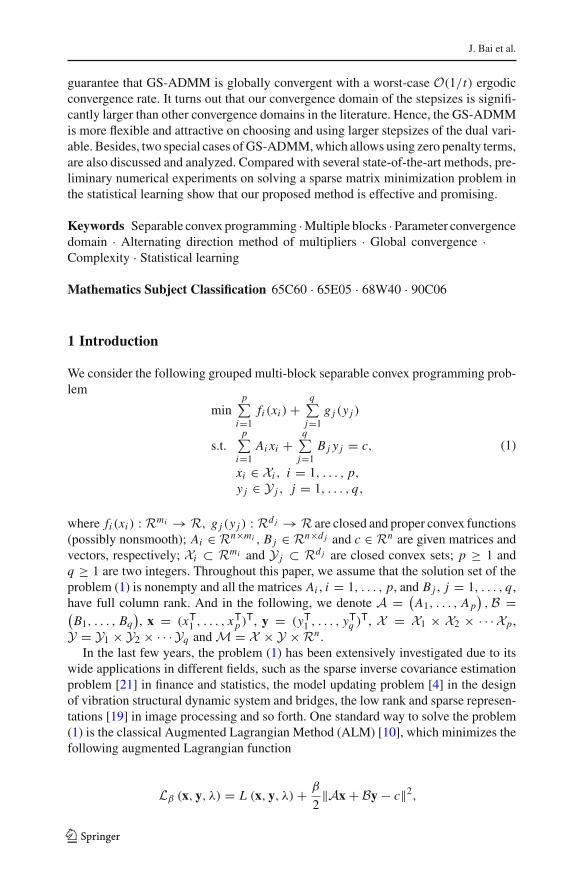
which implies that (61) and (62) hold since ξ1 > 0 and ξ2 > 0.Because (σ1, σ2, τ, s) satisfy (53), we have by Lemma 4 that H is positive definite.

So, it follows from (59) that the sequence {wk} is uniformly bounded. Therefore,there exits a subsequence {wk j } converging to a point w∞ = (x∞, y∞, λ∞) ∈ M. Inaddition, by the definitions of xk , yk and λk in (13) and (14), it follows from (61), (62)

123

J. Bai et al.

and the full column rank assumption of all the matrices Ai and B j that

limk→∞ xk

i − x ki = 0, lim

k→∞ ykj − yk

j = 0 and limk→∞ λk − λk = 0, (64)

for all i = 1, . . . , p and j = 1, . . . , q. So, we have limk→∞wk − wk = 0. Thus, for any

fixed w ∈ M, taking wk j in (16) and letting j go to ∞, we obtain

h(u) − h(u∞) + 〈w − w∞,J (w∞)〉 ≥ 0. (65)

Hence, w∞ ∈ M∗ is a solution point of VI(h,J ,M) defined in (12).Since (59) holds for anyw∗ ∈ M∗, by (59) andw∞ ∈ M∗, for all l ≥ k j , we have

∥∥∥wl − w∞

∥∥∥2

H+ ξ3

∥∥∥Axl + Byl − c

∥∥∥2 + ξ4

∥∥∥yl − yl−1

∥∥∥2

Hy

≤∥∥∥wk j − w∞

∥∥∥2

H+ ξ3

∥∥∥Axk j + Byk j − c

∥∥∥2 + ξ4

∥∥∥yk j − yk j −1

∥∥∥2

Hy.

This together with (62), (64), limj→∞wk j = w∞ and the positive definiteness of H

illustrate liml→∞wl = w∞. Therefore, thewhole sequence {wk} converges to the solution

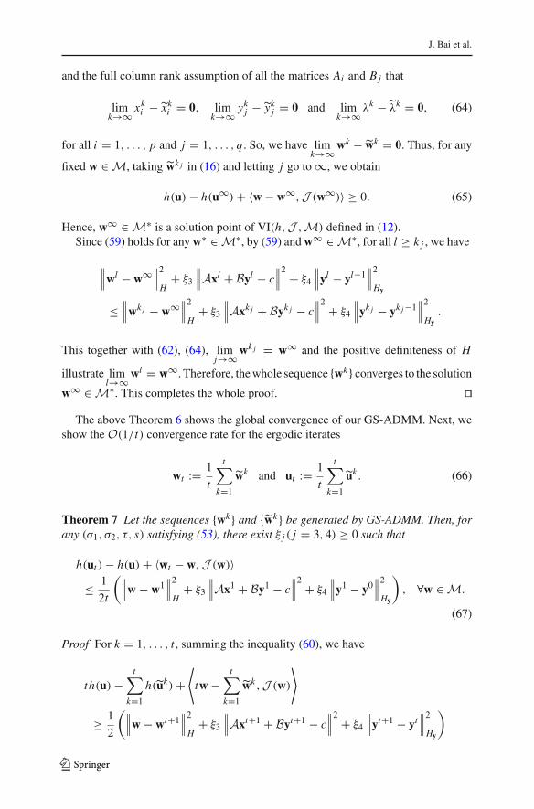
w∞ ∈ M∗. This completes the whole proof. ��The above Theorem 6 shows the global convergence of our GS-ADMM. Next, we

show the O(1/t) convergence rate for the ergodic iterates

wt := 1

t

t∑

k=1

wk and ut := 1

t

t∑

k=1

uk . (66)

Theorem 7 Let the sequences {wk} and {wk} be generated by GS-ADMM. Then, forany (σ1, σ2, τ, s) satisfying (53), there exist ξ j ( j = 3, 4) ≥ 0 such that

h(ut ) − h(u) + 〈wt − w,J (w)〉≤ 1

2t

(∥∥∥w − w1

∥∥∥2

H+ ξ3

∥∥∥Ax1 + By1 − c

∥∥∥2 + ξ4

∥∥∥y1 − y0

∥∥∥2

Hy

)

, ∀w ∈ M.

(67)

Proof For k = 1, . . . , t , summing the inequality (60), we have

th(u) −t∑

k=1

h(uk) +⟨

tw −t∑

k=1

wk,J (w)

⟩

≥ 1

2

(∥∥∥w − wt+1

∥∥∥2

H+ ξ3

∥∥∥Axt+1 + Byt+1 − c

∥∥∥2 + ξ4

∥∥∥yt+1 − yt

∥∥∥2

Hy

)

123


−1

2

(

‖w − w1‖2H + ξ3

∥∥∥Ax1 + By1 − c

∥∥∥2 + ξ4

∥∥∥y1 − y0

∥∥∥2

Hy

)

, ∀w ∈ M.

(68)

Since (σ1, σ2, τ, s) satisfy (53), Hy is positive definite. And by Lemma 4, H is alsopositive definite. So, it follows from (68) that

1

t

t∑

k=1

h(uk) − h(u) +⟨1

t

t∑

k=1

wk − w,J (w)

⟩

≤ 1

2t

(∥∥∥w − w1

∥∥∥2

H+ ξ3

∥∥∥Ax1 + By1 − c

∥∥∥2 + ξ4

∥∥∥y1 − y0

∥∥∥2

Hy

)

, ∀w ∈ M.

(69)

By the convexity of h and (66), we have

h(ut ) ≤ 1

t

t∑

k=1

h(uk).

Then, (67) follows from (69). ��Remark 1 In the above Theorems 6 and 7, we assume the parameters (σ1, σ2, τ, s)satisfy (53). However, because of the symmetric role played by the x and y iteratesin the GS-ADMM, substituting the index k + 1 by k for the x and λ iterates, theGS-ADMM algorithm (7) can be clearly written as

⎧⎪⎪⎪⎪⎪⎪⎪⎪⎪⎪⎪⎪⎪⎪⎪⎪⎪⎨

⎪⎪⎪⎪⎪⎪⎪⎪⎪⎪⎪⎪⎪⎪⎪⎪⎪⎩

For j = 1, 2, . . . , q,

yk+1j = arg min

y j ∈Y j

Lβ(xk, yk1 , . . . , y j , . . . , yk

q , λk− 12 ) + Qk

j (y j ),


2

∥∥∥B j (y j − yk

j )

∥∥∥2,

λk = λk− 12 − sβ(Axk + Byk+1 − c)

For i = 1, 2, . . . , p,

xk+1i = arg min

xi ∈Xi

Lβ(xk1 , . . . , xi , . . . , xk

p, yk+1, λk) + Pk

i (xi ),


2

∥∥Ai (xi − xk

i )∥∥2 ,

λk+ 12 = λk − τβ(Axk+1 + Byk+1 − c).

(70)

So, by applying Theorems 6 and 7 on the algorithm (70), it also converges and has theO(1/t) convergence rate when (σ1, σ2, τ, s) satisfy

σ1 ∈ (p − 1,+∞), σ2 ∈ (q − 1,+∞) and (τ, s) ∈ K, (71)

where

K ={(τ, s) | τ + s > 0, s ≤ 1, −τ 2 − s2 − τ s + τ + s + 1 > 0

}. (72)

123

J. Bai et al.

Hence, the convergence domain K in Theorems 6 and 7 can be easily enlarged to thesymmetric domain, shown in Fig. 2,

G = K ∪ K ={(τ, s) | τ + s > 0, −τ 2 − s2 − τ s + τ + s + 1 > 0

}. (73)

Remark 2 Theorem 6 implies that we can apply the following easily usable stoppingcriterion for GS-ADMM:

max{∥∥∥xk

i − xk+1i

∥∥∥∞ ,

∥∥∥yk

j − yk+1j

∥∥∥∞ ,

∥∥∥Axk+1 + Byk+1 − c

∥∥∥∞

}≤ tol,

where tol > 0 is a given tolerance error. One the other hand, Theorem 7 tells us thatfor any given compact set K ⊂ M, if

η = supw∈K

{

‖w − w1‖2H + ξ3

∥∥∥Ax1 + By1 − c

∥∥∥2 + ξ4

∥∥∥y1 − y0

∥∥∥2

Hy

}

< ∞,

we have

h(ut ) − h(u) + 〈wt − w,J (w)〉 ≤ η

2t,

which shows that GS-ADMM has a worst-caseO(1/t) convergence rate in an ergodicsense.

4 Two special cases of GS-ADMM

Note that in GS-ADMM (7), the two proximal parameters σ1 and σ2 are required tobe strictly positive for the generalized p + q block separable convex programming.However, when taking σ1 = σ2 = 0 for the two-block problem, i.e., p = q = 1,GS-ADMMwould reduce to the scheme (5), which is globally convergent [16]. Suchobservations motivate us to further investigate the following two special cases:

(a) GS-ADMM (7) with p ≥ 1, q = 1, σ1 ∈ (p − 1,∞) and σ2 = 0;(b) GS-ADMM (7) with p = 1, q ≥ 1, σ1 = 0 and σ2 ∈ (q − 1,∞).

4.1 Convergence for the case (a)

The corresponding GS-ADMM for the first case (a) can be simplified as follows:

123


⎧⎪⎪⎪⎪⎪⎪⎪⎪⎪⎪⎨

⎪⎪⎪⎪⎪⎪⎪⎪⎪⎪⎩

For i = 1, 2, . . . , p,

xk+1i = arg min

xi ∈Xi

Lβ

(xk1 , . . . , xi , . . . , xk

p, yk, λk)

+ Pki (xi ),


2

∥∥Ai

(xi − xk

i

)∥∥2 ,

λk+ 12 = λk − τβ

(Axk+1 + Byk − c),

yk+1 = argminy∈Y

Lβ

(xk+1, y, λk+ 1

2

),

λk+1 = λk+ 12 − sβ

(Axk+1 + Byk+1 − c).

(74)

And, the corresponding matrices Q, M, H and G in this case are the following:

Q =[

Hx 0

0 Q

]

, (75)

where Hx is defined in (18) and

Q =[

βBTB −τ BT

−B 1β

I

]

, (76)

M =⎡

⎣I

I−sβB (τ + s)I

⎤

⎦ , (77)

H = QM−1 =

⎡

⎢⎢⎢⎣

Hx (1 − τ s

τ+s

)βBTB − τ

τ+s BT

− ττ+s B 1

(τ+s)β I

⎤

⎥⎥⎥⎦

, (78)

G = Q + QT − MTH M =⎡

⎢⎣

Hx

(1 − s)βBTB (s − 1)BT

(s − 1)B 2−τ−sβ

I

⎤

⎥⎦ . (79)

It can be verified that H in (78) is positive definite as long as

σ1 ∈ (p − 1,+∞), (τ, s) ∈ {(τ, s) | τ + s > 0, τ < 1}.

123

J. Bai et al.

Analogous to (44), we have

1

β‖wk − wk‖2G =

∥∥∥∥∥∥∥∥∥∥∥∥

⎛

⎜⎜⎜⎜⎜⎜⎝

A1

(xk1 − xk+1

1

)

A2

(xk2 − xk+1

2

)

...

Ap

(xk

p − xk+1p

)

⎞

⎟⎟⎟⎟⎟⎟⎠

∥∥∥∥∥∥∥∥∥∥∥∥

2

Hx,0

+ (2 − τ − s)∥∥∥Axk+1 + Byk+1 − c

∥∥∥2 + (1 − τ)

∥∥∥B

(yk − yk+1

)∥∥∥2

+ 2(1 − τ)(Axk+1 + Byk+1 − c

)TB

(yk − yk+1

)

≥ ξ1

p∑

i=1

∥∥∥Ai

(xk

i − xk+1i

)∥∥∥2 + (2 − τ − s)

∥∥∥Axk+1 + Byk+1 − c

∥∥∥2

+ (1− τ)

∥∥∥B

(yk−yk+1

)∥∥∥2 +2(1−τ)

(Axk+1 + Byk+1 − c

)TB

(yk−yk+1

),

(80)

for some ξ1 > 0, since Hx,0 defined in (32) is positive definite. When σ2 = 0, by aslight modification for the proof of Lemma 6, we have the following lemma.

Lemma 7 Suppose τ > −1. The sequence {wk} generated by the algorithm (74)satisfies

(Axk+1 + Byk+1 − c

)TB

(yk − yk+1

)

≥ 1 − s

1 + τ

(Axk + Byk − c

)TB

(yk − yk+1

)− τ

1 + τ

∥∥∥B

(yk − yk+1

)∥∥∥2.

Then, the following two theorems are similar to Theorems 5 and 6.

Theorem 8 Let the sequences {wk} and {wk} be generated by the algorithm (74). Forany

σ1 ∈ (p − 1,+∞) and (τ, s) ∈ K,

where K is given in (8), there exist constants ξi (i = 1, 2) > 0 and ξ3 ≥ 0, such that

∥∥∥wk − wk

∥∥∥2

G≥ ξ1

p∑

i=1

‖Ai

(xk

i − xk+1i

)‖2 + ξ2

∥∥∥Axk+1 + Byk+1 − c

∥∥∥2(81)

+ ξ3

(∥∥∥Axk+1 + Byk+1 − c

∥∥∥2 −


∥∥∥2)

.

123


Proof For any (τ, s) ∈ K, we have τ > −1. Then, by Lemma 7, the inequality (80)and the Cauchy-Schwartz inequality (55), we can deduce that (81) holds with ξ1 givenin (80), ξ2 and ξ3 given in (58) and (57), respectively. ��Theorem 9 Let the sequences {wk} and {wk} be generated by the algorithm (74). Forany

σ1 ∈ (p − 1,+∞) and (τ, s) ∈ K1, (82)

where

K1 ={(τ, s) | τ + s > 0, τ < 1, −τ 2 − s2 − τ s + τ + s + 1 > 0

},

we have

limk→∞

p∑

i=1

∥∥∥Ai

(xk

i − xk+1i

)∥∥∥2 = 0 and lim

k→∞


∥∥∥ = 0, (83)

and there exists a w∞ ∈ M∗ such that limk→∞ wk = w∞.

Proof First, it is clear that Theorem 3 still holds, which, combining with Theorem 8,gives

‖wk+1 − w∗‖2H + ξ3

∥∥∥Axk+1 + Byk+1 − c

∥∥∥2

≤ ‖wk − w∗‖2H + ξ3


∥∥∥2

−ξ1

p∑

i=1

‖Ai

(xk

i − xk+1i

)‖2 − ξ2

∥∥∥Axk+1 + Byk+1 − c

∥∥∥2, ∀w∗ ∈ M∗. (84)

Hence, (83) holds. For (σ1, τ, s) satisfying (82), H in (78) is positive definite. So,by (84), {wk} is uniformly bounded and therefore, there exits a subsequence {wk j }converging to a point w∞ = (x∞, y∞, λ∞) ∈ M. So, it follows from (83) and thefull column rank assumption of all the matrices Ai that

limk→∞ xk

i − x ki = lim

k→∞ xki − xk+1

i = 0 and limk→∞ λk − λk = 0, (85)

for all i = 1, . . . , p. Hence, by limj→∞wk j = w∞ and (83), we have

limj→∞ xk j +1 = x∞ and Ax∞ + By∞ − c = 0,

and therefore, by the full column rank assumption of B and (83),

limj→∞ yk j +1 = lim

j→∞ yk j = y∞.

123

J. Bai et al.

Hence, by (85), we have limj→∞wk j − wk j = 0. Thus, by taking wk j in (16) and letting

j go to ∞, the inequality (65) still holds. Then, the rest proof of this theorem followsfrom the same proof of Theorem 6. ��

Based on Theorem 8 and by a similar proof to those of Theorem 7, we can alsoshow that the algorithm (74) has the worst-case O(1/t) convergence rate, which isomitted here for conciseness.

4.2 Convergence for the case (b)

The corresponding GS-ADMM for the case (b) can be simplified as follows

⎧⎪⎪⎪⎪⎪⎪⎪⎪⎪⎪⎨

⎪⎪⎪⎪⎪⎪⎪⎪⎪⎪⎩

xk+1 = arg minx∈X

Lβ(x, yk, λk)

λk+ 12 = λk − τβ(Axk+1 + Byk − c),

For j = 1, 2, . . . , q,

yk+1j = arg min

y j ∈Y j

Lβ(xk+1, yk1 , . . . , y j , . . . , yk

q , λk+ 12 ) + Qk

j (y j ),


2

∥∥∥B j (y j − yk

j )

∥∥∥2,

λk+1 = λk+ 12 − sβ(Axk+1 + Byk+1 − c).

(86)

In this case, the corresponding matrices Q, M, H and G become Q, M, H and G,which are defined in (19), the lower-right blockof M in (25), (29) and (41), respectively.

In what follows, let us define

vk =(yk

λk

)

and vk =(yk

λk

)

.

Then, by the proof of Theorem 5, we can deduce the following theorem.

Theorem 10 Let the sequences {vk} and {vk} be generated by the algorithm (86). Forany

σ2 ∈ (q − 1,+∞) and (τ, s) ∈ K,

where K is defined in (8), there exist constants ξi (i = 1, 2) > 0 and ξ j ( j = 3, 4) ≥ 0such that

∥∥∥vk − vk

∥∥∥2

G≥ ξ1

q∑

j=1

∥∥∥B j

(yk

j − yk+1j

)∥∥∥2 + ξ2

∥∥∥Axk+1 + Byk+1 − c

∥∥∥2

+ ξ3

(∥∥∥Axk+1 + Byk+1 − c

∥∥∥2 −


∥∥∥2)

+ ξ4

(∥∥∥yk+1 − yk

∥∥∥2

Hy−

∥∥∥yk − yk−1

∥∥∥2

Hy

)

.

123


By slight modifications of the proof of Theorems 6 and 9, we have the followingglobal convergence theorem.

Theorem 11 Let the sequences {wk} and {wk} be generated by the algorithm (74).Then, for any

σ2 ∈ (q − 1,+∞) and (τ, s) ∈ K,

where K is defined in (8), we have

limk→∞

q∑

j=1

∥∥∥B j

(yk

j − yk+1j

)∥∥∥2 = 0 and lim

k→∞


∥∥∥ = 0,

and there exists a w∞ ∈ M∗ such that limk→∞ wk = w∞.

By a similar proof to that of Theorem 7, the algorithm (86) also has the worst-caseO(1/t) convergence rate.

Remark 3 Again, substituting the index k+1 by k for the x andλ iterates, the algorithm(74) can be also written as

⎧⎪⎪⎪⎪⎪⎪⎪⎪⎪⎪⎨

⎪⎪⎪⎪⎪⎪⎪⎪⎪⎪⎩

yk+1 = argminy∈Y

Lβ(xk, y, λk− 12 ),

λk = λk− 12 − sβ(Axk + Byk+1 − c)

For i = 1, 2, . . . , p,

xk+1i = arg min

xi ∈Xi

Lβ(xk1 , . . . , , xi , . . . , xk

p, yk+1, λk) + Pki (xi ),


2

∥∥Ai (xi − xk

i )∥∥2 ,

λk+ 12 = λk − τβ(Axk+1 + Byk+1 − c).

So, by applying Theorem 11 on the above algorithm, we know the algorithm (74) alsoconverges globally when (σ1, τ, s) satisfy

σ1 ∈ (p − 1,+∞), and (τ, s) ∈ K,

where K is given in (72). Hence, the convergence domain K1 in Theorem 9 can beenlarged to the symmetric domain G = K1 ∪K given in (73). By a similar reason, theconvergence domain K in Theorem 11 can be enlarged to G as well.

5 Numerical experiments

In this section, we investigate the performance of the proposedGS-ADMM for solvinga class of sparse matrix minimization problems. All the algorithms are coded andsimulated in MATLAB 7.10(R2010a) on a PC with Intel Core i5 processor(3.3GHz)with 4 GB memory.

123

J. Bai et al.

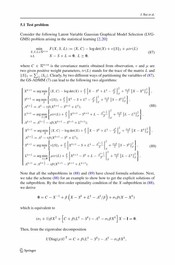
5.1 Test problem

Consider the following Latent Variable Gaussian Graphical Model Selection (LVG-GMS) problem arising in the statistical learning [2,20]:

minX,S,L∈Rn×n

F(X, S, L) := 〈X, C〉 − log det(X) + ν‖S‖1 + μtr(L)

s.t. X − S + L = 0, L 0,(87)

where C ∈ Rn×n is the covariance matrix obtained from observation, ν and μ aretwo given positive weight parameters, tr(L) stands for the trace of the matrix L and‖S‖1 = ∑

i j |Si j |. Clearly, by two different ways of partitioning the variables of (87),the GS-ADMM (7) can lead to the following two algorithms:

⎧⎪⎪⎪⎪⎪⎪⎪⎪⎪⎪⎪⎨

⎪⎪⎪⎪⎪⎪⎪⎪⎪⎪⎪⎩

Xk+1 = argminX

{

〈X, C〉 − log det(X) + β2

∥∥∥X − Sk + Lk − Λk

β

∥∥∥2

F+ σ1β

2

∥∥X − Xk

∥∥2

F

}

,

Sk+1 = argminS

{

ν‖S‖1 + β2

∥∥∥Xk − S + Lk − Λk

β

∥∥∥2

F+ σ1β

2

∥∥S − Sk

∥∥2

F

}

,

Λk+ 12 = Λk − τβ(Xk+1 − Sk+1 + Lk),

Lk+1 = argminL 0

{

μtr(L) + β2

∥∥∥∥Xk+1 − Sk+1 + L − Λ

k+ 12

β

∥∥∥∥

2

F+ σ2β

2

∥∥L − Lk

∥∥2

F

}

,

Λk+1 = Λk+ 12 − sβ(Xk+1 − Sk+1 + Lk+1);

(88)

⎧⎪⎪⎪⎪⎪⎪⎪⎪⎪⎪⎪⎪⎨

⎪⎪⎪⎪⎪⎪⎪⎪⎪⎪⎪⎪⎩

Xk+1 = argminX

{

〈X, C〉 − log det(X) + β2

∥∥∥X − Sk + Lk − Λk

β

∥∥∥2

F+ σ1β

2

∥∥X − Xk

∥∥2

F

}

,

Λk+ 12 = Λk − τβ(Xk+1 − Sk + Lk),

Sk+1 = argminS

{

ν‖S‖1 + β2

∥∥∥∥Xk+1 − S + Lk − Λ

k+ 12

β

∥∥∥∥

2

F+ σ2β

2

∥∥S − Sk

∥∥2

F

}

,

Lk+1 = argminL 0

{

μtr(L) + β2

∥∥∥∥Xk+1 − Sk + L − Λ

k+ 12

β

∥∥∥∥

2

F+ σ2β

2

∥∥L − Lk

∥∥2

F

}

,

Λk+1 = Λk+ 12 − sβ(Xk+1 − Sk+1 + Lk+1).

(89)

Note that all the subproblems in (88) and (89) have closed formula solutions. Next,we take the scheme (88) for an example to show how to get the explicit solutions ofthe subproblem. By the first-order optimality condition of the X -subproblem in (88),we derive

0 = C − X−1 + β(

X − Sk + Lk − Λk/β)

+ σ1β(X − Xk)

which is equivalent to

(σ1 + 1)β X2 +[C + β(Lk − Sk) − Λk − σ1β Xk

]X − I = 0.

Then, from the eigenvalue decomposition

UDiag(ρ)UT = C + β(Lk − Sk) − Λk − σ1β Xk,

123


where Diag(ρ) is a diagonal matrix with ρi , i = 1, . . . , n, on the diagonal, we obtainthat the solution of the X -subproblem in (88) is

Xk+1 = UDiag(γ )UT,

where Diag(γ ) is the diagonal matrix with diagonal elements

γi =−ρi +

√ρ2

i + 4(σ1 + 1)β

2(σ1 + 1)β, i = 1, 2, . . . , n.

On the other hand, the S-subproblem in (88) is equivalent to

Sk+1 = argminS

{

ν‖S‖1 + (σ1+1)β2

∥∥∥S − Xk+Lk+σ1Sk−Λk/β

(σ1+1)

∥∥∥2

F

}

= Shrink(

Xk+Lk+σ1Sk−Λk/β(σ1+1) , ν

(σ1+1)β

),

where Shrink(·, ·) is the soft shrinkage operator (see e.g.[22]). Meanwhile, it is easyto verify that the L-subproblem is equivalent to

Lk+1 = argminL 0

(σ2+1)β2

∥∥L − L

∥∥2

F

= VDiag(max{ρ, 0})V T,

where max{ρ, 0} is taken component-wise and VDiag(ρ)V T is the eigenvalue decom-position of the matrix

L = σ2Lk + Sk+1 + Λk+ 12 /β − Xk+1 − μI/β

(σ2 + 1).

5.2 Numerical results

In the following, we investigate the performance of several algorithms for solvingthe LVGGMS problem, where all the corresponding subproblems can be solved in asimilar way as shown in the above analysis. For all algorithms, the maximal numberof iterations is set as 1000, the starting iterative values are set as (X0, S0, L0,Λ0) =(I, 2I, I, 0), and motivated by Remark 2, the following stopping conditions are used

IER(k) := max{∥∥∥Xk − Xk−1

∥∥∥∞ ,

∥∥∥Sk − Sk−1

∥∥∥∞ ,

∥∥∥Lk − Lk−1

∥∥∥∞

}≤ TOL,

OER(k) := |F(Xk, Sk, Lk) − F∗||F∗| ≤ Tol,

together with CER(k) := ∥∥Xk − Sk + Lk

∥∥

F ≤ 10−4, where F∗ is the approximateoptimal objective function value obtained by running GS-ADMM (88) after 1000

123

J. Bai et al.

iterations. In (87), we set (ν, μ) = (0.005, 0.05) and the given data C is randomlygenerated by the following MATLAB code with m = 100, which are downloadedfrom S. Boyd’s homepage2:

randn(’seed’,0); rand(’seed’,0); n=m; N=10*n;Sinv=diag(abs(ones(n,1))); idx=randsample(nˆ2,0.001*nˆ2);Sinv(idx)=ones(numel(idx),1); Sinv=Sinv+Sinv’;if min(eig(Sinv))<0

Sinv=Sinv+1.1*abs(min(eig(Sinv)))*eye(n);endS=inv(Sinv);D=mvnrnd(zeros(1,n),S,N); C=cov(D);

5.2.1 Performance of different versions of GS-ADMM

In the following, we denote

GS-ADMM (88) by “GS-ADMM-I′′;GS-ADMM (89) by “GS-ADMM-II′′;GS-ADMM (88) with σ2 = 0 by “GS-ADMM-III′′;GS-ADMM (89) with σ1 = 0 by “GS-ADMM-IV′′.

First, wewould like to investigate the performance of the above different versions ofGS-ADMM for solving the LVGGMS problemwith variance of the penalty parameterβ. The results are reported in Table 1 with TOL = Tol = 1.0 × 10−7, and (τ, s) =(0.8, 1.17). For GS-ADMM-I and GS-ADMM-II, (σ1, σ2) = (2, 3). Here, “Iter” and“CPU” denote the iteration number and the CPU time in seconds, and the bold letterindicates the best result of each algorithm. From Table 1, we can observe that:

– Both the iteration number and the CPU time of all the algorithms have a similarchanging pattern, which decreases originally and then increases along with thedecrease of the value of β.

– For the same value of β, the results of GS-ADMM-III are slightly better than otheralgorithms in terms of the iteration number, CPU time, and the feasibility errorsCER, IER and OER.

– GS-ADMM-III with β = 0.5 can terminate after 579 iterations to achieve thetolerance 10−7, while the other algorithms with β = 0.5 fail to achieve thistolerance within given number of iterations.

In general, the algorithm (88) with β = 0.06 performs better than other cases. Hence,in the following experiments for GS-ADMM, we adapt GS-ADMM-III with defaultβ = 0.06. Also note that σ2 = 0, which is not allowed by the algorithms discussed in[15].

2 http://web.stanford.edu/~boyd/papers/admm/covsel/covsel_example.html.

123

http://web.stanford.edu/~boyd/papers/admm/covsel/covsel_example.html


Table 1 Numerical results of GS-ADMM-I, II, III and IV with different β

Iter(k) CPU(s) CER IER OER

GS-ADMM-I/β

0.5 1000 15.29 7.2116e−8 5.0083e−6 3.2384e−10

0.2 493 8.58 1.4886e−8 9.8980e−8 5.7847e−11

0.1 254 4.24 1.6105e−8 9.7867e−8 5.6284e−11

0.08 202 3.27 1.7112e−8 9.8657e−8 5.6063e−11

0.07 175 3.03 1.7548e−8 9.7091e−8 5.4426e−11

0.06 146 2.42 1.9200e−8 9.9841e−8 5.4499e−11

0.05 115 1.84 1.9174e−8 8.8302e−8 4.4919e−11

0.03 112 2.21 1.7788e−7 9.9591e−8 2.2472e−11

0.01 270 4.50 6.4349e−7 9.9990e−8 2.5969e−10

0.006 424 7.57 1.0801e−6 9.8883e−8 5.0542e−10

0.004 604 10.74 1.6490e−6 9.9185e−8 8.7172e−10

GS-ADMM-II/β

0.5 1000 15.80 8.8857e−8 3.2511e−6 4.0156e−10

0.2 603 11.35 3.7706e−9 9.9070e−8 1.2204e−12

0.1 312 4.93 6.0798e−9 9.9239e−8 2.3994e−12

0.08 250 4.40 7.1384e−9 9.6234e−8 2.8127e−12

0.07 217 3.42 8.2861e−9 9.8471e−8 3.1878e−12

0.06 183 3.09 9.7087e−8 9.8298e−8 3.4898e−12

0.05 147 2.85 1.1335e−8 9.1450e−8 3.3405e−12

0.03 114 1.85 1.5606e−7 9.1283e−8 1.9479e−11

0.01 271 4.70 6.2003e−7 9.6960e−8 2.4594e−10

0.006 424 7.38 1.0774e−6 9.8852e−8 5.0224e−10

0.004 604 10.01 1.6461e−6 9.9114e−8 8.6812e−10

GS-ADMM-III/β

0.5 579 9.36 1.2740e−8 9.9818e−8 5.2821e−11

0.2 247 5.52 1.2043e−8 9.6354e−8 4.5217e−11

0.1 125 2.14 1.1737e−8 9.5170e−8 3.6207e−11

0.08 97 1.55 1.2078e−8 9.7603e−8 2.8773e−11

0.07 82 1.36 1.1854e−8 9.5322e−8 1.6215e−11

0.06 69 1.27 1.2680e−8 8.2352e−8 1.5087e−11

0.05 71 1.40 9.1560e−8 9.8745e−8 8.1869e−12

0.03 110 1.71 1.8118e−7 9.4257e−8 2.7549e−11

0.01 271 4.46 6.3390e−7 9.7803e−8 2.5210e−10

0.006 424 6.92 1.0856e−6 9.9123e−8 5.0717e−10

0.004 604 10.11 1.6527e−6 9.9275e−8 8.7303e−10

GS-ADMM-IV/β

0.5 1000 15.76 7.1259e−8 2.6323e−6 6.9956e−12

0.2 587 9.08 3.8200e−9 9.9214e−8 1.3291e−12

0.1 304 4.80 6.0296e−9 9.6197e−8 2.4309e−12

123

J. Bai et al.

Table 1 continued

Iter(k) CPU(s) CER IER OER

0.08 243 4.91 7.2062e−9 9.4484e−8 2.8670e−12

0.07 211 3.25 8.1772e−9 9.4133e−8 3.1477e−12

0.06 177 2.81 9.9510e−9 9.6911e−8 3.5342e−12

0.05 140 3.07 1.3067e−8 9.9446e−8 3.6691e−12

0.03 115 1.80 1.6886e−7 9.5844e−8 2.1829e−11

0.01 271 4.67 6.2006e−7 9.7151e−8 2.4927e−10

0.006 424 6.94 1.0758e−6 9.8755e−8 5.0454e−10

0.004 604 10.21 1.6454e−6 9.9088e−8 8.6995e−10

For each method, the bold number is the smallest (best) value in that column

Second, we investigate how the stepsizes (τ, s) ∈ G with different values wouldaffect the performance of GS-ADMM-III. Table 2 reports the comparison results withvariance of (τ, s) for TOL = Tol = 1.0×10−5. One obvious observation fromTable 2is that both the iteration number and the CPU time decrease along with the increaseof s (or τ ) for fixed value of τ (or s), which indicates that the stepsizes of (τ, s) ∈ Gcould influence the performance of GS-ADMM significantly. In addition, the resultsin Table 2 also indicate that usingmore flexible but with both relatively larger stepsizesτ and s of the dual variables often gives the best convergence speed. Comparing allthe reported results in Table 2, by setting (τ, s) = (0.9, 1.09), GS-ADMM-III givesthe relative best performance for solving the problem (87).

5.2.2 Comparison of GS-ADMM with other state-of-the-art algorithms

In this subsection, we would like to carry out some numerical comparison of solvingthe problem (87) by using GS-ADMM-III and the other four methods:

– The Proximal Jacobian Decomposition of ALM [17] (denoted by “PJALM”);– The splitting method in [14] (denoted by “HTY”);– The generalized parametrized proximal point algorithm [1] (denoted by “GR-PPA”).

– The twisted version of the proximal ADMM [23] (denoted by “T-ADMM”).

We set (τ, s) = (0.9, 1.09) for GS-ADMM-III and the parameter β = 0.05 for allthe comparison algorithms. The default parameter μ = 2.01 and H = βI are usedfor HTY [14]. As suggested by the theory and numerical experiments in [17], theproximal parameter is set as 2 for PJALM. As shown in [1], the relaxation factor ofGR-PPA is set as 1.8 and other default parameters are chosen as

(σ1, σ2, σ3, s, τ, ε) =(

0.178, 0.178, 0.178, 10,

√5 − 1

2,

√5 − 1

2

)

.

For T-ADMM, the symmetric matrices therein are chosen as M2 = M2 = vI withv = β and the correction factor is set as a = 1.6 [23]. The results obtained by the above

123


Table 2 Numerical results of GS-ADMM-III with different stepsizes (τ, s)

(τ, s) Iter(k) CPU(s) CER IER OER

(1, −0.8) 256 4.20 9.8084e−5 7.8786e−6 1.1298e−7

(1, −0.6) 144 2.39 5.7216e−5 9.9974e−6 3.8444e−8

(1, −0.4) 105 1.80 3.5144e−5 9.7960e−6 1.3946e−8

(1, −0.2) 84 1.45 2.3513e−5 9.3160e−6 6.4220e−9

(1, 0) 70 1.14 1.7899e−5 9.4261e−6 3.9922e−9

(1, 0.2) 61 0.98 1.3141e−5 8.9191e−6 1.7780e−9

(1, 0.4) 54 0.88 1.0549e−5 9.1564e−6 4.6063e−10

(1, 0.6) 49 0.82 9.0317e−5 9.4051e−6 2.7938e−9

(1, 0.8) 49 0.80 3.5351e−5 8.0885e−6 1.4738e−9

(−0.8, 1) 229 3.91 9.9324e−5 8.4462e−6 1.9906e−7

(−0.6, 1) 127 2.06 6.1118e−5 9.6995e−6 7.8849e−8

(−0.4, 1) 96 1.61 3.4111e−5 9.6829e−6 2.7549e−8

(−0.2, 1) 79 1.30 2.2004e−5 9.6567e−6 1.2015e−8

(0, 1) 67 1.16 1.6747e−5 9.9244e−6 6.2228e−9

(0.2, 1) 59 0.93 1.2719e−5 9.4862e−6 2.9997e−9

(0.4, 1) 53 0.88 1.0253e−5 9.3461e−6 3.4811e−10

(0.6, 1) 49 0.85 8.0343e−6 8.8412e−6 2.9837e−9

(0.8, 1) 49 0.81 3.3831e−6 8.1998e−6 2.1457e−9

(1.6, −0.3) 60 0.99 1.2111e−5 9.4583e−6 1.1705e−9

(1.6, −0.6) 74 1.22 1.8012e−5 9.6814e−6 2.7562e−9

(1.5, −0.8) 97 1.68 3.1310e−5 9.8972e−6 1.4911e−8

(1.3, 0.3) 50 0.83 8.5476e−6 8.9655e−6 3.4389e−10

(0.2, 0.5) 87 1.44 2.7160e−5 9.4503e−6 1.7906e−8

(0.4, 0.9) 56 0.98 1.1060e−5 9.1081e−6 1.7179e−9

(0.8, 1.17) 49 0.86 1.5419e−6 8.5023e−6 2.5529e−9

(0, 1.618) 50 0.90 5.5019e−6 8.6980e−6 1.4722e−9

(0.9, 1.09) 49 0.78 1.4874e−6 8.4766e−6 2.2194e−9

(0.1, 0.1) 229 4.42 9.8698e−5 8.3622e−6 2.3575e−7

(0.2, 0.2) 130 2.32 5.5559e−5 9.9888e−6 7.5859e−8

(0.3, 0.3) 97 1.75 3.4344e−5 9.9362e−6 2.8190e−8

(0.4, 0.4) 79 1.43 2.4256e−5 9.8539e−6 1.2790e−8

(0.5, 0.5) 68 1.15 1.6805e−5 9.2144e−6 5.5121e−9

(0.6, 0.6) 59 0.98 1.3862e−5 9.7793e−6 2.8580e−9

(0.7, 0.7) 53 0.91 1.1091e−5 9.6433e−6 3.9013e−12

(0.8, 0.8) 49 0.84 8.4235e−6 8.9432e−6 3.0519e−9

(0.9, 0.9) 49 0.83 3.4493e−6 8.1314e−6 1.8888e−9

Bold numbers in the first and second rows indicate that the best results obtained with changing either τ ors; Bold numbers in the third row indicate that the best results obtained with changing both τ and s; Boldnumbers in the last row indicate that the best results obtained when both τ and s belong to (0, 1)

123

J. Bai et al.

Table 3 Comparative results of different algorithms under different tolerances

TOL Tol I ter(k) CPU(s) CER IER OER

GS-ADMM-III

1e−3 1e−7 33 0.46 8.3280e−5 2.5770e−4 4.0973e−9

1e−12 83 1.16 9.5004e−9 1.0413e−8 8.3240e−13

1e−6 1e−8 58 0.84 8.3812e−7 9.0995e−7 7.6372e−11

1e−14 108 1.55 1.0936e−10 1.2072e−10 9.5398e−15

1e−9 1e−7 97 1.39 7.7916e−10 8.5759e−10 6.8775e−14

1e−15 118 1.72 1.8412e−11 2.0361e−11 6.6557e−16

PJALM

1e−3 1e−7 62 0.88 9.6422e−5 3.6934e−5 5.8126e−8

1e−12 187 2.74 9.4636e−9 3.4868e−9 9.4447e−13

1e−6 1e−8 111 1.67 2.4977e−6 9.4450e−7 4.1335e−10

1e−14 249 3.63 1.0173e−10 3.7225e−11 8.6506e−15

1e−9 1e−7 205 3.06 2.5369e−9 9.3210e−10 2.4510e−13

1e−15 276 4.08 1.4143e−11 5.2002e−11 6.6543e−16

HTY

1e−3 1e−7 62 0.85 4.8548e−5 1.7123e−5 9.3737e−8

1e−12 176 2.64 2.7059e−9 9.7709e−10 9.1783e−13

1e−6 1e−8 92 1.35 2.7184e−6 9.6661e−7 4.0385e−9

1e−14 223 3.15 1.1042e−10 4.0226e−11 9.3091e−15

1e−9 1e−7 176 2.78 2.7059e−9 9.7709e−10 9.1783e−13

1e−15 243 3.70 2.8377e−11 1.0533e−11 4.4329e−16

GR-PPA

1e−3 1e−7 61 0.82 7.4082e−5 3.3954e−5 1.5195e−9

1e−12 127 1.84 5.8944e−8 1.6729e−7 1.3001e−13

1e−6 1e−8 108 1.52 5.5130e−7 6.2676e−7 3.4315e−11

1e−14 172 2.56 2.9521e−10 8.3742e−10 8.8742e−16

1e−9 1e−7 167 2.42 5.3963e−10 7.3383e−10 3.7050e−14

1e−15 172 2.41 2.9521e−10 8.3742e−10 8.8742e−16

T-ADMM

1e−3 1e−7 40 0.55 9.8495e−5 1.2096e−4 2.7440e−8

1e−12 112 1.53 7.1036e−9 4.8224e−9 8.9763e−13

1e−6 1e−8 72 1.02 1.3128e−6 8.9570e−7 2.3510e−10

1e−14 147 2.12 7.4334e−11 5.0156e−11 9.7617e−15

1e−9 1e−7 125 1.70 1.3053e−9 8.8746e−10 1.5974e−13

1e−15 160 2.01 1.3669e−11 9.4374e−12 6.6557e−16

Bold numbers indicate that they are the best results for each tolerance compared with other methods

algorithms under different tolerances are reported in Table 3. With fixed toleranceTOL = 10−9 and Tol = 10−15, the convergence behavior of the error measurementsIER(k) and OER(k) by the five algorithms using different starting points are shown

123


0 50 100 150 200 250 30010−15

10−10

10−5

100

105

Itera

tive

erro

r IER

(k)

Iter (k)

0 50 100 150 200 250 30010−20

10−15

10−10

10−5

100

Rel

ativ

e re

sidu

al O

EB(k

)

Iter (k)

GS−ADMM−IIIPJALMHTYGR−PPAT−ADMM


Fig. 3 Convergence curves of IER and OER with initial values (X0, S0, L0, Λ0) = (I, 2I, I, 0)

0 50 100 150 200 250 30010−15

10−10

10−5

100

105

Itera

tive

erro

r IER

(k)

Iter (k)

0 50 100 150 200 250 30010−20

10−15

10−10

10−5

100

Rel

ativ

e re

sidu

al O

EB(k

)

Iter (k)



Fig. 4 Convergence curves of IER and OER with initial values (X0, S0, L0, Λ0) = (I, I, 0, 0)

in Figs. 3, 4 and 5. From Table 3 and Figs. 3, 4 and 5, we may have the followingobservation:

123

J. Bai et al.

0 50 100 150 200 250 30010 −15

10 −10

10 −5

10 0

10 5

Itera

tive

erro

r IER

(k)

Iter (k)

0 50 100 150 200 250 30010−20

10−15

10−10

10−5

100

105

Rel

ativ

e re

sidu

al O

EB(k

)

Iter (k)



Fig. 5 Convergence curves of IER and OER with initial values (X0, S0, L0, Λ0) = (I, 4I, 3I, 0)

– Under all different tolerances, GS-ADMM-III performs significantly better thanother four algorithms in both the number of iterations and CPU time.

– GR-PPA is slightly better than PJALM and HTY, and T-ADMM outperformsPJALM, HTY and GR-PPA.

– the convergence curves in Figs. 3, 4 and 5 illustrate that using different startingpoints, GS-ADMM-III also converges fastest among the comparing methods.

All these numerical results demonstrate the effectiveness and robustness of GS-ADMM-III, which is perhaps due to the symmetric updating of the Lagrangemultipliers and the proper choice of the stepsizes.

6 Conclusion

Since the direct extension of ADMM in a Gauss–Seidel fashion for solving the three-block separable convex optimization problem is not necessarily convergent analyzedby Chen et al. [3], there has been a constantly increasing interest in developing andimproving the theory of the ADMM for solving the multi-block separable convexoptimization. In this paper, we propose an algorithm, called GS-ADMM, which couldsolve the general model (1) by taking advantages of the multi-block structure. Inour GS-ADMM, the Gauss–Seidel fashion is taken for updating the two groupedvariables, while the block variables within each group are updated in a Jacobi scheme,which would make the algorithm more be attractive and effective for solving bigsize problems. We provide a new convergence domain for the stepsizes of the dualvariables, which is significantly larger than the convergence domains given in the

123


literature. Global convergence as well as the O(1/t) ergodic convergence rate of theGS-ADMM is established. In addition, two special cases of GS-ADMM,which allowsone of the proximal parameters to be zero, are also discussed.

This paper simplifies the analysis in [16] and provides an easy way to analyze theconvergence of the symmetric ADMM. Our preliminary numerical experiments showthat with proper choice of parameters, the performance of the GS-ADMM could bevery promising. Besides, from the presented convergence analysis, we can see that thetheories in the paper can be naturally extended to use more general proximal terms,such as letting Pk

i (xk) := β2 ‖xi − xk

i ‖Pi and Qkj (y j ) := β

2 ‖y j − ykj ‖Q j in (7), where

Pi and Qi are matrices such that Pi � (p − 1)ATi Ai and Q j � (q − 1)BT

j B j forall i = 1, . . . , p and j = 1, . . . , q. Finally, the different ways of partitioning thevariables of the problem also gives the flexibility of GS-ADMM.

Acknowledgements The authors would like to thank the anonymous referees for providing very construc-tive comments. Jianchao Bai also wish to thank Prof. Defeng Sun at National University of Singapore forhis valuable discussions on ADMM and Prof. Pingfan Dai at Xi’an Jiaotong University for discussion onan early version of the paper.

References

1. Bai, J.C., Li, J.C., Li, J.F.: A novel parameterized proximal point algorithm with applications in statis-tical learning. Optimization Online, March (2017) http://www.optimization-online.org/DB_HTML/2017/03/5901.html

2. Chandrasekaran, V., Parrilo, P.A., Willsky, A.S.: Latent variable graphical model selection via convexoptimization. Ann. Stat. 40, 1935–1967 (2012)

3. Chen, C.H., He, B.S., Ye, Y.Y., Yuan, X.M.: The direct extension of ADMM for multi-block mini-mization problems is not necessarily convergent. Math. Program. 155, 57–79 (2016)

4. Dong, B., Yu, Y., Tian, D.D.: Alternating projection method for sparse model updating problems. J.Eng. Math. 93, 159–173 (2015)

5. Fortin, M., Glowinski, R.: Augmented Lagrangian Methods: Applications to the Numerical Solutionof Boundary-Value Problems, pp. 299–331. North-Holland, Amsterdam (1983)

6. Facchinei, F., Pang, J.S.: Finite-Dimensional Variational Inequalities and Complementarity Problems.Springer Ser. Oper. Res. 1, Springer, New York (2003)

7. Fortin, M.: Numerical Methods for Nonlinear Variational Problems. Springer, New York (1984)8. Glowinski, R.,Marrocco, A.: Approximation paréléments finis d’rdre un et résolution, par pénalisation-

dualité d’une classe de problèmes deDirichlet non linéaires. Rev. Fr. Autom. Inform. Rech. Opér. Anal.Numér. 2, 41–76 (1975)

9. Gu, Y., Jiang, B., Han, D.: A semi-proximal-based strictly contractive Peaceman-Rachford splittingmethod. arXiv:1506.02221 (2015)

10. Hestenes, M.R.: Multiplier and gradient methods. J. Optim. Theory Appl. 4, 303–320 (1969)11. He, B.S., Yuan, X.M.: On theO(1/n) convergence rate of the Douglas–Rachford alternating direction

method. SIAM J. Numer. Anal. 50, 700–709 (2012)12. He, B.S., Liu, H.,Wang, Z.R., Yuan, X.M.: A strictly contractive Peaceman–Rachford splitting method

for convex programming. SIAM J. Optim. 24, 1011–1040 (2014)13. He, B.S., Hou, L.S., Yuan, X.M.: On full Jacobian decomposition of the augmented Lagrangianmethod

for separable convex programming. SIAM J. Optim. 25, 2274–2312 (2015)14. He, B.S., Tao, M., Yuan, X.M.: A splitting method for separable convex programming. IMA J. Numer.

Anal. 31, 394–426 (2015)15. He, B.S., Yuan,X.M.: Block-wise alternating directionmethod ofmultipliers formultiple-block convex

programming and beyond. SIAM J. Comput. Math. 1, 145–174 (2015)16. He, B.S., Ma, F., Yuan, X.M.: Convergence study on the symmetric version of ADMMwith larger step

sizes. SIAM J. Imaging Sci. 9, 1467–1501 (2016)

123

http://www.optimization-online.org/DB_HTML/2017/03/5901.html

http://www.optimization-online.org/DB_HTML/2017/03/5901.html

http://arxiv.org/abs/1506.02221

J. Bai et al.

17. He, B.S., Xu, H.K., Yuan, X.M.: On the proximal Jacobian decomposition of ALM for multiple-blockseparable convexminimization problems and its relationship toADMM. J. Sci. Comput. 66, 1204–1217(2016)

18. He, B.S.: On the convergence properties of alternating direction method of multipliers. Numer. Math.J. Chin. Univ. (Chine. Ser.) 39, 81–96 (2017)

19. Liu, Z.S., Li, J.C., Li, G., Bai, J.C., Liu, X.N.: A new model for sparse and low-rank matrix decompo-sition. J. Appl. Anal. Comput. 7, 600–616 (2017)

20. Ma, S.Q.: Alternating proximal gradient method for convexminimization. J. Sci. Comput. 68, 546–572(2016)

21. Rothman, A.J., Bickel, P.J., Levina, E., Zhu, J.: Sparse permutation invariant covariance estimation.Electron. J. Stat. 2, 494–515 (2008)

22. Tao, M., Yuan, X.M.: Recovering low-rank and sparse components of matrices from incomplete andnoisy observations. SIAM J. Optim. 21, 57–81 (2011)

23. Wang, J.J., Song,W.: An algorithm twisted from generalized ADMM for multi-block separable convexminimization models. J. Comput. Appl. Math. 309, 342–358 (2017)

123

generalized symmetric admm for separable convex …hozhang/papers/gs-admm.pdf · generalized...

Documents