1

Generalized Tree-Based Wavelet TransformIdan Ram, Michael Elad, Senior Member, IEEE, and Israel Cohen, Senior Member, IEEE

Abstract—In this paper we propose a new wavelet trans-form applicable to functions defined on high dimensional data,weighted graphs and networks. The proposed method generalizesthe Haar-like transform proposed in [1], and can also constructdata adaptive orthonormal wavelets beyond Haar. It is definedvia a hierarchical tree, which is assumed to capture the geometryand structure of the input data, and is applied to the data usinga modified version of the common one-dimensional (1D) waveletfiltering and decimation scheme. The adaptivity of this waveletscheme is obtained by permutations derived from the tree andapplied to the approximation coefficients in each decompositionlevel, before they are filtered. We show that the proposedtransform is more efficient than both the 1D and two-dimensional(2D) separable wavelet transforms in representing images. Wealso explore the application of the proposed transform to imagedenoising, and show that combined with a subimage averagingscheme, it achieves denoising results which are similar to thoseobtained with the K-SVD algorithm.

Index Terms—Wavelet transform, Hierarchical trees, Efficientsignal representation, Image denoising.

I. INTRODUCTION

Most traditional signal processing methods are designedfor data defined on regular Euclidean grids. Developmentof comparable methods capable of handling non-uniformlysampled signals, data defined on graphs or “point clouds”,is important and very much needed. Many signal processingproblems involve inference of an unknown scalar target func-tion defined on such data. For example, function denoisinginvolves estimating such a scalar function from its noisyversion. A different example is function inpainting whichinvolves estimating missing samples of a function from itsknown samples. A major challenge in processing functions ontopologically complicated data, is to find efficient methods torepresent and learn them.

Many signal processing techniques are based on transformmethods, which represent the input data in a new basis, beforeanalyzing or processing it. One of the most successful typesof transforms, which has been proven to be a very usefultool for signal and image processing, is wavelet analysis[2]. A major advantage of wavelet methods is their abilityto simultaneously localize signal content in both space andfrequency. This property allows them to compactly representsignals such as 1D steps or images with edges, whose primaryinformation content lies in localized singularities. Moreover,

I. Ram and I. Cohen are with the Department of Electrical Engi-neering, Technion – Israel Institute of Technology, Technion City, Haifa32000, Israel. E-mail addresses: idanram@tx.technion.ac.il (I. Ram), ico-hen@ee.technion.ac.il (I. Cohen); tel.: +972-4-8294731; fax: +972-4-8295757.M. Elad is with the Department of Computer Science, Technion – IsraelInstitute of Technology, Technion City, Haifa 32000, Israel. E-mail address:elad@cs.technion.ac.il

This research was partly supported by the ISF grant no. 1031/08 and bythe European Communitys FP7-FET program, SMALL project, under grantagreement no. 225913.

wavelet methods represent such signals much more compactlythan either the original domain or transforms with global basiselements such as the Fourier transform. We aim at extendingthe wavelet transform to irregular, non-Euclidean spaces, andthus obtain a transform that efficiently represents functionsdefined on such data.

Several extensions of the wavelet transform, operating ongraphs and high dimensional data, have already been proposed.The wavelet transforms proposed in [3], [4] and [5] wereapplied to the data points themselves, rather than functions de-fined on the data. Other methods took different approaches toconstruct wavelets applied to functions on the data. Maggioniand Coifman [6] and Hammond et al. [7] proposed waveletsbased on diffusion operators and the graph Laplacian [8], [9],respectively. Jansen et al. [10] proposed three methods whichwere based on a variation of the lifting scheme [11], [12].Gavish et al. [1] assumed that the geometry and structure ofthe input data are captured in a hierarchical tree. Then, givensuch a tree, they built a data adaptive Haar-like orthonormalbasis for the space of functions over the data set. This basis,can be seen as a generalization of the one proposed in [13] forbinary trees. Our proposed method generalizes the algorithmin [1].

We note that the wavelet transforms proposed in [14], and[15], which are defined on images, also share some similaritieswith our proposed algorithm. These methods employ pairingor reordering of wavelet coefficients in the decompositionschemes in order to adapt to their input images. In fact, theeasy path wavelet transform proposed in [15], which onlyrecently has come to our attention, employs a decompositionscheme which is very similar to ours. Constraining our algo-rithm to a regular data grid and using the same starting pointand search neighborhood as the ones employed in [15], bothalgorithms essentially coincide. Nevertheless, our approachis more general, as it tackles the more abstract problem ofdevising a transform for point clouds or high-dimensionalgraph-data, whereas [15] concentrates on images.

In this paper we introduce a generalized tree-based wavelettransform (GTBWT). This method is an extension of the Haar-like transform introduced by Gavish et al [1], which can alsoconstruct data adaptive orthonormal wavelets beyond Haar. Wefirst show that the transform of Gavish et al., when derivedfrom a full binary tree, can be applied to a function over thedata set using a modified version of the common 1D Haarwavelet filtering and decimation scheme. In each level of thiswavelet decomposition scheme, a permutation derived fromthe tree is applied to the approximation coefficients, beforethey are filtered. Then we show how this scheme can beextended to work with different wavelet filters, and explainhow to construct the data driven-hierarchical tree employedby the extended scheme.

2

The construction of each coarse level of the tree involvesfinding a path which passes through the set of data pointsin the finer level. The points order in this path defines thepermutation applied to the approximation coefficients of thefiner level in the wavelet decomposition scheme. We proposea path constructed by starting from a random point, and thencontinue from each point to its nearest neighbor accordingto some distance measure, visiting each point only once.The corresponding permutation increases the regularity of thepermuted approximation coefficients signal, and therefore itis more efficiently (sparsely) represented using the wavelettransform.

Next we show empirically that the proposed scheme ismore efficient than both the common 1D and 2D separablewavelet transforms in representing images. Finally, we explorethe application of the proposed transform to image denoising,and show that combined with a proposed subimage averagingscheme, it achieves denoising results similar to the onesobtained with the K-SVD algorithm [16].

The paper is organized as follows: In Section II we describehow the Haar-like basis introduced in [1] is derived from a fullbinary tree representation of the data. We also describe howsuch a tree may be constructed. In Section III we introducethe generalized tree-based wavelet transform. We also explorethe efficiency with which this transform represents an image.In Section IV we explore the application of our proposedalgorithm to image denoising. We also describe the subimageaveraging scheme and present some experimental results. Wesummarize the paper in Section V.

II. TREE-BASED HAAR WAVELETS

Let X = {x1, ...,xN} be the dataset we wish to analyze,where the samples xi ∈ Rn may be points in high dimension,or feature points associated with the nodes of a weighted graphor network. Also, let f : X → R be a scalar function definedon the dataset, and let V = {f |f : X → R} be the space ofall functions on the dataset. Here we use the following innerproduct with the space V :

〈f, g〉 =N∑

j=1

f(xj)g(xj). (1)

which is different from the one used by Gavish et al. [1], sinceit does not contain a normalizing factor before the sum.

We note that when the dataset is a weighted graph, but nofeature points are available, the diffusion map framework [17],[18] can be employed in order to obtain such points from thegraph. The Euclidean distance between the points producedby this framework approximates the ”diffusion distance” [17],[18], which describes the relationship between the graph nodesin terms of their connectivity.

Gavish et al. assume that the geometry and structure of thedata X are captured by one or several hierarchical trees. Theydo not insist on any specific construction method for thesetrees, but only that they will be balanced [1]. Given such a tree,they construct a multiscale wavelet-like orthonormal basis forthe space V . They start by showing that such a tree induces amulti-resolution analysis with an associated Haar-like wavelet.

Let ` = 1, . . . , L denote the level in the tree, with ` = 1being the root and ` = L being the lowest level, where eachsample xj is a single leaf. Also, let V ` denote the space offunctions constant on all folders (subtrees) at level `, and let1X denote a constant function on X with the value 1. ThenV 1 = SpanR{1X}, V L = V and by construction

V 1 ⊂ ... ⊂ V ` ⊂ V `+1 ⊂ ... ⊂ V L = V. (2)

Now, let W ` (1 ≤ ` < L) be the orthogonal complementof V ` in V `+1. Then, the space of all functions V can bedecomposed as

V = V L =

[L−1⊕

`=1

W `

] ⊕V 1. (3)

Before describing how the multiscale orthonormal basis isconstructed given a hierarchical tree, we first describe howsuch a tree can be constructed from the data. Here we focuson the case of complete full binary trees and the correspondingorthonormal bases. For the case of more general trees and Haarlike bases, the reader may refer to [1]. Let c`

j denote the j-thpoint at level ` of the tree, where cL

j = xj , and let P` and p`

denote a set and a vector containing point indices, respectively.Also, let w(·, ·) be a distance measure in Rn, and let W` be adistance matrix associated with the `-th level of the tree, wherew`

i,j = w(c`i , c

`j). The distance function describes the first-

order interaction between data-points, and therefore it shouldbe chosen so as to capture some notion of similarity betweenthem, which would be meaningful to the application at hand.A complete full binary tree can be constructed from the dataaccording to Algorithm 1. An example for such a tree is shownin Fig. 1.

In the case of a complete full binary tree, the Haar-likebasis constructed from the tree is essentially the standardHaar basis which we denote {ψj}N

j=1. The adaptivity of thetransform is obtained by the fact that this basis is used torepresent a permuted version of the signal f , which is moreefficiently represented by the Haar basis than f itself. Thepermutation is derived from the tree, and is dependent on thedata X. Let p denote a vector of length N , which containsthe indices of the points xj , in the order determined by thelowest level of the fully constructed tree. For example, forthe tree in Fig. 1, p = [1, 3, 4, 8, 2, 5, 6, 7]T . Also let fp bethe signal f permuted according to the vector p. The waveletcoefficients can be calculated by the inner products 〈fp, ψj〉,or by applying the 1D wavelet filtering and decimation schemewith the Haar wavelet filters on fp. Similarly, the inversetransform is calculated by applying the inverse Haar transformon the wavelet coefficients, and reordering the produced vectorso as to cancel the index ordering in p. We hereafter term thescheme described above as tree-based Haar wavelet transform,and we show next that it can be extended to operate withgeneral wavelet filters.

III. GENERALIZED TREE-BASED WAVELETS

A. Generalized tree construction and transform

The above-described building process of the tree can bepresented a little differently. In every level ` of the tree, we

3

Task: Construct a complete full binary tree fromthe data X.Parameters: We are given the points {xj}N

j=1 andthe distance function w.Initialization: Set cL

j = xj as the tree leaves.Main Iteration: Perform the following steps for ` =L, . . . , 2:• Construct a distance matrix W`, where

w`i,j = w(c`

i , c`j).

• Set P` = ∅.• Group the points in level ` in pairs by repeat-

ing N/21+L−` times:– Choose a random point c`

j0 , j0 /∈ P`, andupdate P` = P` ∪ {j0}.

– Pair c`j0 with the point c`

j1 , where j1 =minj /∈P`

w`j0,j .

– Update P` = P` ∪ {j1}.• Place in a vector p` the reordered point in-

dices of P`.• Construct the coarse level `− 1 from the finer

level ` by replacing each pair c`i and c`

j withthe mean point 1√

2[c`

i + c`j ].

Output: The tree node points c`j and the vectors

p` containing the points order in each tree level.

Algorithm 1: Complete full binary tree construction from the data X.

1=� 11c

2=� 21c 2

2c

3=�

4=�

31c 3

3c 32c 3

4c

41c 4

3c 44c 4

8c 42c 4

5c 46c 4

7c

1x 3x 4x 8x 2x 5x 6x 7x

Fig. 1: An illustration of a complete full binary tree.

first construct a distance matrix W` using the mean pointsc`

j and the distance function w. Then we group in pairs thepoints c`

j , according to the weights in W`, as described inAlgorithm 1. Next we place the pairs of column vectors oneafter the other in a matrix Cp

` of size n×N/2L−`, and keepthe indices of the points in their new order in a vector p` oflength N/2L−`. For example in level ` = 3 of the tree in Fig.1, Cp

3 = [c31, c

33, c

32, c

34] and p3 = [1, 3, 2, 4]T .

Now let h = 1√2

[1, 1]T and g = 1√2

[−1, 1]T be the Haar

wavelet decomposition filters, and let h = 1√2

[1, 1]T and

g = 1√2

[1,−1]T be the Haar wavelet reconstruction filters.We notice that replacing each pair by its mean point can bedone by filtering the rows of Cp

` with the low pass filter hT ,followed by decimation of the columns of the outcome by afactor of 2. For example, the points c1

2 and c22 in level ` = 2

of the tree in Fig. 1 are obtained by filtering the rows of Cp3

Task: Apply L − 1 levels of tree-based waveletdecomposition to the signal f .Parameters: We are given the signal f , the vectors{p`}L

`=2, and the filters h and g .Initialization: Set aL = f .Main Iteration: Perform the following steps for ` =L, . . . , 2:• Construct the operator P` that reorders its

input vector according to the indices in p`.• Apply P` to a` and receive ap

` .• Filter ap

` with h and decimate the result by 2to receive a`−1.

• Filter ap` with g and decimate the result by 2

to receive d`−1.Output: The approximation coefficients a1 anddetail coefficients {d`}L−1

`=1 corresponding to f .

Algorithm 2: Tree-based wavelet decomposition algorithm.

h

g

2↓

2↓

P�a� 1a −�1d −� h

g

2↓

2↓

1P −� 2a −�2d −�pa� 1

pa −�Fig. 2: Two single-level tree-based wavelet decomposition steps

described above with the filter hT , and keeping the first andthird columns of the produced matrix. Effectively this meansthat the approximation coefficients corresponding to a single-level Haar decomposition are calculated for each row of thematrix Cp

` .Next let f = [f(x1), . . . , f(xN )]T , and let a` and d` denote

the approximation and detail coefficient vectors, respectively,received for f at level `, where aL = f . Also, let P` denote alinear operator that reorders a vector according to the indicesin p`. Then, applying the Haar transform derived from thetree to f can be carried out according to the decompositionalgorithm in Algorithm 2. Fig. 2 describes two single-leveldecomposition steps carried out according to Algorithm 2. Wenote that here the adaptivity of the transform is related tothe permutations applied to the coefficients a` in every levelof the tree. In fact, without the operator P` applied in eachlevel, the decomposition scheme of Algorithm 2 reduces to thatof the common 1D orthogonal wavelet transform. Also, sincepermutation of points is a unitary transform, the describedtransform remains unitary.

Finally, let the linear operator P−1` reorder a vector so as to

cancel the ordering done by P`. Then the inverse transform iscarried out using the reconstruction algorithm in Algorithm 3.Fig. 3 describes two single-level reconstruction steps carriedout according to Algorithm 3.

We next wish to extend the scheme described above to workwith general wavelet filters. This requires modifying the treeconstruction by replacing the Haar filters by different wavelet

4

Task: Reconstruct the signal f based on a multi-level tree-based wavelet decomposition.Parameters: We are given the approximation anddetail coefficients a1 and {d`}L−1

`=1 , the vectors{p`}L

`=2, and the filters h and g .Main Iteration: Perform the following steps for ` =1, . . . , L− 1:• Interpolate a` by a factor of 2 and filter the

result with h.• Interpolate d` by a factor of 2 and filter the

result with g.• Sum the results of the two previous steps to

receive ap`+1.

• Construct the operator P−1`+1 that reorders its

input vector so as to cancel the index orderingin p`+1.

• Apply P−1`+1 to ap

`+1 and receive a`+1.Output: The reconstructed signal f .

Algorithm 3: Tree-based wavelet reconstruction algorithm.

h

g

2↑

2↑

11P−

−� 1a −�2a −�2d −� h

g

2↑

2↑

1P−� a�1d −�1

pa −� pa�Fig. 3: Two single-level tree-based wavelet reconstruction steps

filters and changing the manner in which the points c`j are

ordered in each level of the tree.We note that when filters other than Haar are used in the

tree construction scheme described above, each point in thecoarse level ` − 1 is calculated as a weighted mean of morethan two points from the finer level `, where the coefficientsin h serve as the weights. Therefore, the resultant graph isno longer a tree but rather a rooted L-partite graph, whichis a graph that contains L disjoint sets of vertices so that notwo vertices within the same set are adjacent. As the waveletscheme described above was originally designed with the Haarwavelet filters, and in order to avoid cumbersome distinctionbetween trees and L-partite graphs, with a small abuse ofterminology we will hereafter refer to the latter also as trees.An example of such a ”generalized” tree, is shown in Fig. 4.

The wavelet decomposition and reconstruction schemescorresponding to each generalized tree are those described inAlgorithms 2 and 3, with the necessary change of waveletfilters type and index vectors p` to the ones used in theconstruction of the tree. We next propose a method to orderthe points in each level of the generalized trees.

B. Smoothing a`

We wish to order the points in each level of a tree ina manner which results in an efficient representation of theinput signal by the tree-based wavelets. More specifically, we

1=� 11c

2=� 21c 2

2c

3=�

4=�

31c 3

3c 32c 3

4c

1x 3x 2x 5x 4x 8x 6x 7x

41c 4

3c 42c 4

5c 44c 4

8c 46c 4

7c

Fig. 4: An illustration of a ”generalized” tree.

Task: Construct of a ”generalized” tree from thedata X.Parameters: We are given the points {xj}N

j=1 andthe weight function w .Initialization: Set cL

j = xj as the tree leaves.Main Iteration: Perform the following steps for ` =L, . . . , 2:• Construct a distance matrix W`, where

w`i,j = w(c`

i , c`j).

• Choose a random point c`j0 and set P` =

{j0}.• Reorder the points c`

j so that they will form asmooth path by repeating N/2L−` − 1 times:– Set j1 = minj /∈P`

w`j0,j and update P` =

P` ∪ {j1}.– Set j0 = j1.

• Place in a vector p` the reordered point in-dices of P`.

• Order the points c`j according to the indices in

p` and place them in a matrix Cp` .

• Obtain the points c`−1j by:

– Apply the filter hT to the matrix Cp` .

– Decimate the columns of the outcome by afactor of 2.

Output: The tree node points c`j and the vectors

p` containing the points order in each tree level.

Algorithm 4: Construction of a ”generalized” tree from the data X.

want the transformed signal to contain a small number of largecoefficients, i.e. to be sparse. The wavelet transform is knownto produce a small number of large coefficients when it isapplied to piecewise regular signals [2]. Thus, we would likethe operator P`, applied to a`, to produce a signal which is asregular as possible. When the signal f is known, the optimalsolution would be to apply a simple sort operation on thecorresponding coefficients a`, obtained in each level. However,since we are interested in the case where f is not necessarilyknown (such as in the case where f is noisy, or has missingvalues), we would try to find a suboptimal ordering operationin each level `, using the feature points c`

j . We assume thatunder the distance measure w(·, ·), proximity between the twopoints c`

i and c`j suggests proximity between the coefficients

a`(i) and a`(j). Thus, we would try to reorder the points

5

c`j so that they will form a smooth path, hoping that the

corresponding reordered 1D signal ap` will also be smooth.

The “smoothness” of a 1D signal y of length N can bemeasured using its total variation

‖y‖V =N∑

j=2

|y(j)− y(j − 1)|. (4)

By analogy, we measure the ”smoothness” of the path Cp` by

the measure

Cp`,V =

N∑

j=2

w(c`j , c

`j−1). (5)

We notice that smoothing the path Cp` comes down to finding

the shortest path that passes through the set of points c`j ,

visiting each point only once. This can be regarded as aninstance of the traveling salesman problem [19], which canbecome very computationally exhaustive for large sets ofpoints. A simple approximate solution is to start from arandom point, and then continue from each point to its nearestneighbor, not visiting any point twice. As it turns out, orderingthe points c`

j in this manner indeed results in an efficientrepresentation of the input signal.

A generalized tree construction, which employs the pro-posed point ordering method is summarized in Algorithm 4.Fig. 4 shows an example of ”generalized” tree which maybe obtained with Algorithm 4 using a filter h of length 4and disregarding boundary issues in the different levels. Weterm the filtering schemes described in Algorithms 2 and 3combined with the tree construction described in Algorithm 4generalized tree-based wavelet transform (GTBWT).

An interesting question is whether the wavelet schemedescribed above represents the signal f more efficiently thanthe common 1D and 2D separable wavelet transforms. Here,we measure efficiency by the m-term approximation error, i.e.the error obtained when representing a signal with m non-zerotransform coefficients.

Before relating to this question, we first explain how thewavelet scheme described above can be applied to images.Let F be a grayscale image of size

√N × √N and let f be

its column stacked representation, i.e. f is a vector of lengthN containing individual pixel intensities. Then we first needto extract the feature points xi from the image, which will belater used to construct the tree. Let fi be the i-th sample in f ,then we choose the point xi associated with it as the 9×9 patcharound the location of fi in the image F. We next constructseveral trees, each with a different wavelet filter, according tothe scheme described above. We choose the weight functionw to be the squared Euclidean distance, i.e. the (i, j) elementin W` is

w`i,j = ‖c`

i − c`j‖2. (6)

We use the transforms corresponding to these trees to obtainm-term approximations of a column stacked version of the128 × 128 image shown in Fig. 7(a) (the center of the Lenaimage). The approximations, shown in Fig. 5, were carriedout by keeping the highest coefficients (in absolute value) inthe different transform domains. We compare these results be-tween themselves, and to the m-term approximations obtained

with the common 1D and the 2D separable wavelet transforms(the latter applied to the original image) corresponding to thesame wavelet filters. The quality of the results is measured inpeak signal-to-noise ratio (PSNR), defined by

PSNR = 20 log

255√1N

∑Ni=1

(fi − fi

)2

(7)

where fi is the estimate of fi. It can be seen that thegeneralized tree-based wavelet transform outperforms the twoother transforms for all the wavelet filters that have been used.It can also be seen that the PSNR gap in the first thousandsof coefficients increases with number of vanishing momentsof the wavelet filters. Further, Figure 5(d) shows that thegeneralized tree-based wavelet results obtained with the db4and db8 filters are close, and better than the ones obtainedwith the Haar filter.

Before concluding this section, we are interested to see howthe basis elements of the proposed wavelet transform look like.Each basis element is obtained by setting the correspondingtransform coefficient to 1 and all the other coefficients to zero,and applying the inverse transform. Unlike the case of common1D wavelet bases, the series of data derived permutationsapplied to the reconstructed coefficients in the different stagesof the inverse transform, result in basis functions which adaptthemselves to the input signal f .

As a first example, we examine the basis elements obtainedfor the synthetic image of size 64 × 64, shown in Fig 6(a).The image contains in its middle a square rotated in an angleof 45 degrees. We visualize the basis elements as images byreshaping them to the size of the input image. Figs 6(b)-(n) show some of the basis elements corresponding to thesynthetic image, and obtained with the Symmlet 8 filter. Thefigures show two scaling functions from level ` = 1, andtwo wavelet basis functions from each level ` = 1, . . . , 12,all corresponding to the two largest coefficients in the samelevel. We note that the reason we have more than one scalingfunction and one wavelet basis element in the coarsest level` = 1 is related to our implementation of the transform. We usesymmetric padding in the signal boundaries before applyingthe wavelet filters, which slightly increases the number ofcoefficients (and corresponding basis elements) obtained ineach level of the tree. It can be seen that the scaling functionsand wavelets in the low levels of the tree (` = 1, . . . , 4)represent the low frequency information in the image, i.e.smooth versions of the rectangle. It can also be seen that thewavelet functions represent finer edges as the level of the treeincreases, and that they successfully manage to capture edgeswhich are not aligned with the vertical and horizontal axes.

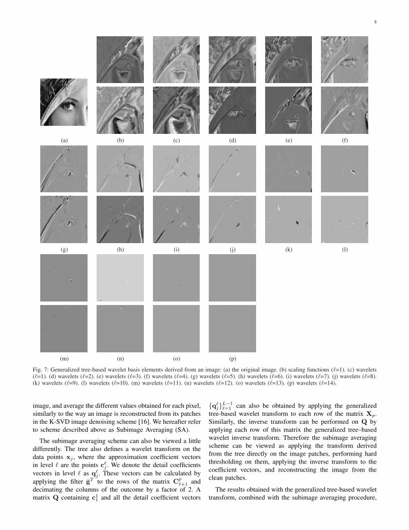
We next examine the wavelet basis elements correspondingto the image in Fig. 7(a), obtained with the Symmlet 8 filter.Figs. 7(b)-(p) show two scaling functions from level ` = 1,and two wavelet basis functions from each level ` = 1, . . . , 14,all corresponding to the two largest coefficients in the samelevel. It can be seen that the basis functions adapt to the shapesin the images. Here again the scaling functions and waveletsin the low levels of the tree (` = 1, . . . , 4) represent the low

6

0 2000 4000 6000 8000 1000010

15

20

25

30

35

40

45

50

55

# Coefficients

PS

NR

generalized tree−based (solid)common 1D (dotted)2D separable (dashed)

0 2000 4000 6000 8000 1000010

15

20

25

30

35

40

45

50

55

# Coefficients

PS

NR

generalized tree−based (solid)common 1D (dotted)2D separable (dashed)

(a) (b)

0 2000 4000 6000 8000 1000010

15

20

25

30

35

40

45

50

55

# Coefficients

PS

NR

generalized tree−based (solid)common 1D (dotted)2D separable (dashed)

0 500 1000 1500 2000 2500 3000 3500 400020

22

24

26

28

30

32

34

36

38

40

# Coefficients

PS

NR

db1 (squares)db4 (circles)db8 (diamonds)

(c) (d)

Fig. 5: m-term approximation results (PSNR in dB) for the generalized tree-based, common 1D and 2D separable wavelet transforms,obtained with different wavelet filters: (a) Daubechies 1 (Haar). (b) Daubechies 4. (c) Daubechies 8. (d) Comparison between the generalizedtree-based wavelet results obtained with the different filters.

frequency information in the image, and the wavelet functionsrepresent finer edges in the image as the level of the treeincreases. We next present the application of the generalizedtree-based wavelet transform to image denoising.

IV. IMAGE DENOISING USING THE GENERALIZEDTREE-BASED WAVELET TRANSFORM

A. The Basics

Let F be an image of size√

N × √N , and let F be its

noisy version:F = F + Z. (8)

Z is a matrix of size√

N × √N which denotes an additivewhite Gaussian noise independent of F with zero mean andvariance σ2. Also, let f and f be the column stacked represen-tations of F and F, respectively. Our goal is to reconstruct ffrom f using the generalized tree-based wavelet transform. Tothis end, we first extract the feature points xi from F similarlyto the way they were extracted from F in the previous section.Let fi be the i-th sample in f , then here we choose the pointxi associated with it as the 9 × 9 patch around the locationof fi in the image F. We note that since different features areused for the clear and noisy images, the corresponding treesderived from these images will also be different. Nevertheless,

it was shown in [20], [21], [22] that the distance between thenoisy patches xi and xj is a good predictor for the similaritybetween the clear versions of their middle pixels fi and fj .This means that the tree construction is roughly robust tonoise, and that the obtained tree will capture the geometryand structure of the clear image quite well. We will furtherdiscuss the noise robustness of the algorithm in Section IV-C.

We next construct the tree according to the scheme de-scribed in Algorithm 4, where the dissimilarity between thepoints c`

i and c`j in level ` is again measured by the squared

Euclidean distance between them, which can be found in the(i, j) location in W`.

Similarly to Gavish et al. [1], we use an approach whichresembles the “cycle spinning” method [23] in order tosmooth the image denoising outcome. This means that werandomly construct 10 different trees, utilize the transformscorresponding to each of them to denoise f , and average theproduced images. Each level of a random tree is constructedby choosing the first point at random, and then continue fromeach point xj0 to its nearest neighbor xj1 with a probabilityp1 ∝ exp(−‖xj0−xj1‖2/ε), or to its second nearest neighborxj2 with a probability p2 ∝ exp(−‖xj0 − xj2‖2/ε), wherehere we set ε = 0.1.

The denoising itself is performed by applying the proposed

7

(a) (b) (c) (d) (e) (f) (g)

(h) (i) (j) (k) (l) (m) (n)

Fig. 6: Generalized tree-based wavelet basis elements derived from a synthetic image: (a) the original image. (b) scaling functions (`=1). (c)wavelets (`=1). (d) wavelets (`=2). (e) wavelets (`=3). (f) wavelets (`=4). (g) wavelets (`=5). (h) wavelet (`=6). (i) wavelet (`=7). (j) wavelet(`=8). (k) wavelets (`=9). (l) wavelets (`=10). (m) wavelets (`=11). (n) wavelets (`=12).

wavelet transform (derived from the tree of f ) on f , using hardthresholding on the transform coefficients, and computing theinverse transform.

In order to assess the performance of the proposed denoisingalgorithm we first apply it, using different wavelet filters, to anoisy version of the image shown in Fig. 7(a). For each of thetransforms we perform 5 experiments for different realizationsof noise with standard deviation σ = 25 and average theresults – these averages are given in Table I. We note thatthe denoising thresholds were manually found to producegood denoising results, as the theoretical wavelet thresholdσ√

2 loge N led to poorer results, with PSNR values whichwere lower by about 0.6 dB. It can be seen that better resultsare obtained with the Symmlet wavelets, and that generallybetter results are obtained with wavelets with a high number ofvanishing moments. It can also be seen that all the transformsrequire about 320 coefficients to represent the image (for eachof the 10 results produced by the different trees) which isabout 2 percents of the number of coefficients required in theoriginal space.

We next apply the proposed scheme with the Symmlet 8wavelet to noisy versions of the images Lena and Barbara,with noise standard deviation σ = 25 and PSNR of 20.17dB. We note that this time we use patches of size 13 × 13and perform only one experiment for each image, for onerealization of noise. The clear, noisy and recovered imagescan be seen in Fig. 8. For comparison, we also apply tothe two images the denoising scheme of Elad et al. [16],which utilize the K-SVD algorithm [24]. We chose to compareour results to the ones obtained by this scheme, as it alsoemploys an efficient representation of the image content, and isone of many state-of-the-art image denoising algorithms [25],

[26], which are based on sparse and redundant representations[27]. However, we note that this scheme is based on efficientrepresentations of individual fixed size image patches, whileour tree-based approach attempts at an image-adaptive efficientrepresentation of the whole image using multiple scales. ThePSNR of the results obtained with the proposed scheme andthe K-SVD algorithm are shown in Table II. It can be seen thatthe results obtained by our algorithm are inferior compared tothe ones obtained with the K-SVD. We next try to improvethe results produced by our proposed scheme by adding anaveraging element into it, which is also a variation on the“cycle spinning” method.

B. Subimage averaging

Let Xp be an n × (√

N − √n + 1)2 matrix, containing

column stacked versions of all the√

n×√n patches xi insidethe image. When we built a tree for the image, we assumed thateach patch is associated only with its middle pixel. Thereforethe tree was associated with the signal composed of the middlepoints in the patches, which is the middle row of Xp, andthe transform was applied to this signal. However, we canalternatively choose to associate all the patches with a pixellocated in a different position, for example the top rightpixel in each patch. Since the whole patches are used in theconstruction of the tree, effectively this means that the treecan be associated with any one of the n signals located in therows of Xp. These signals are the column stacked versions ofthe n subimages of size (

√N −√n + 1)× (

√N −√n + 1),

whose top right pixel reside in the top right√

n×√n patch inthe image. We next apply the generalized tree-based wavelettransform denoising scheme to each of these n signals. Wethen plug each denoised subimage into its original place in the

8

(a) (b) (c) (d) (e) (f)

(g) (h) (i) (j) (k) (l)

(m) (n) (o) (p)

Fig. 7: Generalized tree-based wavelet basis elements derived from an image: (a) the original image. (b) scaling functions (`=1). (c) wavelets(`=1). (d) wavelets (`=2). (e) wavelets (`=3). (f) wavelets (`=4). (g) wavelets (`=5). (h) wavelets (`=6). (i) wavelets (`=7). (j) wavelets (`=8).(k) wavelets (`=9). (l) wavelets (`=10). (m) wavelets (`=11). (n) wavelets (`=12). (o) wavelets (`=13). (p) wavelets (`=14).

image, and average the different values obtained for each pixel,similarly to the way an image is reconstructed from its patchesin the K-SVD image denoising scheme [16]. We hereafter referto scheme described above as Subimage Averaging (SA).

The subimage averaging scheme can also be viewed a littledifferently. The tree also defines a wavelet transform on thedata points xj , where the approximation coefficient vectorsin level ` are the points c`

j . We denote the detail coefficientsvectors in level ` as q`

j . These vectors can be calculated byapplying the filter gT to the rows of the matrix Cp

`+1 anddecimating the columns of the outcome by a factor of 2. Amatrix Q containing c1

1 and all the detail coefficient vectors

{q`j}L−1

`=1 can also be obtained by applying the generalizedtree-based wavelet transform to each row of the matrix Xp.Similarly, the inverse transform can be performed on Q byapplying each row of this matrix the generalized tree–basedwavelet inverse transform. Therefore the subimage averagingscheme can be viewed as applying the transform derivedfrom the tree directly on the image patches, performing hardthresholding on them, applying the inverse transform to thecoefficient vectors, and reconstructing the image from theclean patches.

The results obtained with the generalized tree-based wavelettransform, combined with the subimage averaging procedure,

9

TABLE I: Denoising results of a noisy version of the image in Fig.7(a) (σ = 25, input PSNR=20.18 dB), obtained using the GTBWT,with and without subimage averaging (SA), and with differentwavelet filters. Also shown is the average number of coefficients(#coeffs.) used by each scheme to represent an image.

GTBWT with SAwavelet type PSNR [dB] #coeffs PSNR [dB] #coeffsdb1 (Haar) 28.19 303.28 29.05 349.02

db4 28.5 307.62 29.37 341.25db8 28.49 384.08 29.33 403.2

sym2 28.45 293.84 29.25 326.48sym4 28.51 308.6 29.38 349.81sym8 28.55 342.76 29.39 392.77

TABLE II: Denoising results (PSNR in dB) of noisy versions of theimages Barbara and Lena (σ = 25, input PSNR=20.17 dB) obtainedwith: 1) GTBWT with a Symmlet 8 filter with subimage averaging(SA) and without it. 2) with the K-SVD algorithm.

Image GTBWT GTBWT + SA K-SVDLena 30.3 31.21 31.32

Barbara 28.94 29.82 29.62

for the noisy version of the image in Fig. 7(a) are shown inTable I. It can be seen that this procedure increases the PSNRof the results by about 0.85 dB. We note that since we use9 × 9 patches, each of the 10 images averaged in the cyclespinning procedure is reconstructed from 81 subimages, and itcan be seen that on average about 360 transform coefficientsare required to represent each one of these subimages. Thusthe number of transform coefficients required to represent eachsubimage is slightly higher than the one required to representan image when the subimage averaging is not used, but is stillmuch lower than the number required in the original space.

We also applied the proposed denoising scheme to thenoisy Lena and Barbara images. The reconstructed imagesare shown in Figs. 8(d) and (h), and Table II shows thecorresponding PSNR results. It can be seen that the resultsobtained with the proposed algorithm for the Lena image arenow closer to the ones received by the K-SVD algorithm, andthe results obtained for the Barbara image are better than theones obtained with the K-SVD algorithm.

We note that only a subset of design parameters has beenexplored when we applied the proposed image denoisingalgorithm. These design parameters include the patch size, thewavelet filter type (we have not explored biorthogonal waveletfilters at all), and the number of trees averaged by the cyclespinning method. They also include the number of nearestneighbors to choose from in the construction process of eachlevel of these trees, and the parameter ε used to determine theprobabilities of choosing them. We believe that better resultsmay be achieved with the adequate design parameters, andtherefore more tests need to be performed in order to searchfor the parameters which optimize the performance of thealgorithm. We also note that the use of the proposed sub-image averaging scheme is not restricted to the generalizedtree-based wavelet transform. This scheme may be used toimprove the denoising results obtained with different methodswhich use distance matrices similar to the one employed here.

TABLE III: Denoising results (PSNR in dB) of noisy versions ofthe images Barbara and Lena (σ = 25, input PSNR=20.17 dB)obtained using the GTBWT with subimage averaging. The treeswere constructed using patches obtained from the noisy (1 iter),original (clean) and reconstructed (2 iters) images.

Image 1 iter 2 iters cleanLena 31.21 31.34 32.25

Barbara 29.82 29.71 30.61

C. Robustness to noise

We wish to explore the robustness of the generalized tree-based wavelet denoising scheme to the noise in the points xj .More specifically we wish to check how using cleaner imagepatches will affect the denoising results. Here we obtained”clean” patches from a noisy image by applying our denoisingscheme once, and using the patches from the reconstructedimage in a second iteration of the denoising algorithm fordefining the permutations. For comparison we also used cleanpatches from the original clean image in our denoising scheme,and regarded the obtained results as oracle estimates.

We applied the GTBWT denoising schemes, obtained withpatches from the clean and reconstructed images, to the noisyBarbara and Lena images. The results obtained with theSymmlet 8 filter and with subimage averaging are shown inTable III. It can be seen that large improvements of about1 dB for the Lena image and 0.8 dB for the Barbara imageare obtained with clean patches. Applying 2 iterations of thedenoising algorithm slightly improves the results of the Lenaimage by about 0.13 dB. However, applying 2 iterations ofthe denoising algorithm to the Barbara image degrades theobtained results by about 0.11 dB. This degradation probablyresults from oversmoothing of the patches of the reconstructedimage, which leads to a loss of details. A choice of a differentthreshold in the denoising algorithm applied in first iteration,or a different method to clean the patches altogether, may leadto improved denoising results.

V. CONCLUSION

We have proposed a new wavelet transform applicable tographs and high dimensional data. This transform is an exten-sion of the multiscale harmonic analysis approach proposedby Gavish et al. [1]. We have shown a relation between thetransform suggested by Gavish et al. and 1D Haar waveletfiltering, and extended the former scheme so it will use generalwavelet filters. We demonstrated the ability of the generalizedscheme to represent images more efficiently than the common1D and separable 2D wavelet transforms. We have also shownthat our proposed scheme can be used for image denoising, andthat combined with a subimage averaging scheme it achievesdenoising results which are close to the state-of-the-art.

In our future work plans, we intend to consider the followingissues:

1) Seek ways to improve the method that reorders theapproximation coefficients in each level of the tree,replacing the proposed nearest neighbor method.

2) Extend this work to redundant wavelets.

10

(a) (b) (c) (d)

(e) (f) (g) (h)

Fig. 8: Denoising results of noisy versions of the images Barbara and Lena (σ = 25, input PSNR=20.17 dB) obtained with GTBWT witha Symmlet 8 filter with subimage averaging (SA) and without it: (a) Original Lena. (b) Noisy Lena (20.17 dB). (c) Lena denoised usingGTBWT (30.3 dB). (d) Lena denoised using GTBWT with sub image averaging (31.21 dB) (e) Original Barbara. (f) Noisy Barbara (20.17dB). (g) Barbara denoised using GTBWT (28.94 dB). (h) Barbara denoised using GTBWT with sub image averaging (29.82 dB).

3) Improve the image denoising results by using two iter-ations with different threshold settings, and by consid-ering spatial proximity as well in the tree construction.

ACKNOWLEDGEMENTS

The authors thank Ron Rubinstein and Matan Gavish forthe fruitful discussions and ideas which helped in developingthe presented work. The authors also thank the anonymousreviewers for their helpful comments.

REFERENCES

[1] M. Gavish, B. Nadler, and R. R. Coifman, “Multiscale wavelets ontrees, graphs and high dimensional data: Theory and applications tosemi supervised learning,” in Proceedings of the 27th InternationalConference on machine Learning, 2010.

[2] S. Mallat, A Wavelet Tour of Signal Processing, The Sparse Way.Academic Press, 2009.

[3] F. Murtagh, “The Haar wavelet transform of a dendrogram,” Journal ofClassification, vol. 24, no. 1, pp. 3–32, 2007.

[4] A. B. Lee, B. Nadler, and L. Wasserman, “Treelets-An adaptive multi-scale basis for sparse unordered data,” Annals, vol. 2, no. 2, pp. 435–471,2008.

[5] G. Chen and M. Maggioni, “Multiscale geometric wavelets for theanalysis of point clouds,” in Information Sciences and Systems (CISS),2010 44th Annual Conference on. IEEE, 2010, pp. 1–6.

[6] R. R. Coifman and M. Maggioni, “Diffusion wavelets,” Applied andComputational Harmonic Analysis, vol. 21, no. 1, pp. 53–94, 2006.

[7] D. K. Hammond, P. Vandergheynst, and R. Gribonval, “Wavelets ongraphs via spectral graph theory,” Applied and Computational HarmonicAnalysis, 2010.

[8] F. R. K. Chung, “Spectral graph theory,” vol. 92, CBMS RegionalConference Series in Mathematics. AMS Bookstore, 1997.

[9] U. Von Luxburg, “A tutorial on spectral clustering,” Statistics andComputing, vol. 17, no. 4, pp. 395–416, 2007.

[10] M. Jansen, G. P. Nason, and B. W. Silverman, “Multiscale methods fordata on graphs and irregular multidimensional situations,” Journal of theRoyal Statistical Society: Series B (Statistical Methodology), vol. 71,no. 1, pp. 97–125, 2009.

[11] W. Sweldens, “The lifting scheme: A custom-design construction ofbiorthogonal wavelets,” Applied and Computational Harmonic Analysis,vol. 3, no. 2, pp. 186–200, 1996.

[12] ——, “The lifting scheme: A construction of second generationwavelets,” SIAM Journal on Mathematical Analysis, vol. 29, no. 2, p.511, 1998.

[13] K. Egiazarian and J. Astola, “Tree-structured Haar transforms,” Journalof Mathematical Imaging and Vision, vol. 16, no. 3, pp. 269–279, 2002.

[14] S. Mallat, “Geometrical grouplets,” Applied and Computational Har-monic Analysis, vol. 26, no. 2, pp. 161–180, 2009.

[15] G. Plonka, “The Easy Path Wavelet Transform: A New Adaptive WaveletTransform for Sparse Representation of Two-Dimensional Data,” Mul-tiscale Modeling & Simulation, vol. 7, p. 1474, 2009.

[16] M. Elad and M. Aharon, “Image denoising via sparse and redundantrepresentations over learned dictionaries,” IEEE Transactions on ImageProcessing, vol. 15, no. 12, pp. 3736–3745, 2006.

[17] R. R. Coifman and S. Lafon, “Diffusion maps,” Applied and Computa-tional Harmonic Analysis, vol. 21, no. 1, pp. 5–30, 2006.

[18] S. Lafon, Y. Keller, and R. R. Coifman, “Data fusion and multicue datamatching by diffusion maps,” IEEE Transactions on pattern analysisand machine intelligence, vol. 28, no. 11, pp. 1784–1797, 2006.

[19] T. H. Cormen, Introduction to algorithms. The MIT press, 2001.[20] A. Buades, B. Coll, and J. M. Morel, “A review of image denoising

algorithms, with a new one,” Multiscale Modeling and Simulation, vol. 4,no. 2, pp. 490–530, 2006.

[21] A. D. Szlam, M. Maggioni, and R. R. Coifman, “Regularization ongraphs with function-adapted diffusion processes,” The Journal of Ma-chine Learning Research, vol. 9, pp. 1711–1739, 2008.

[22] A. Singer, Y. Shkolnisky, and B. Nadler, “Diffusion interpretation ofnon-local neighborhood filters for signal denoising,” SIAM J. on Imag.Sci, vol. 2, no. 1, pp. 118–139, 2009.

[23] R. R. Coifman and D. L. Donoho, Wavelets and Statistics. Springer-Verlag, 1995, ch. Translation-invariant de-noising, pp. 125–150.

[24] M. Aharon, M. Elad, and A. Bruckstein, “K-SVD: An algorithm fordesigning overcomplete dictionaries for sparse representation,” IEEETransactions on signal processing, vol. 54, no. 11, p. 4311, 2006.

11

[25] J. Mairal, M. Elad, G. Sapiro et al., “Sparse representation for colorimage restoration,” IEEE Transactions on Image Processing, vol. 17,no. 1, p. 53, 2008.

[26] J. Mairal, F. Bach, J. Ponce, G. Sapiro, and A. Zisserman, “Non-localsparse models for image restoration,” in Computer Vision, 2009 IEEE12th International Conference on. IEEE, 2010, pp. 2272–2279.

[27] A. M. Bruckstein, D. L. Donoho, and M. Elad, “From sparse solutions ofsystems of equations to sparse modeling of signals and images,” SIAMreview, vol. 51, no. 1, pp. 34–81, 2009.