generalrelativity - uzh · generalrelativity autumn semester 2016 prof. philippe jetzer original...
TRANSCRIPT

Physik-Institut der Universität Zürichin conjunction with ETH Zürich
General Relativity
Autumn semester 2016
Prof. Philippe Jetzer
Original version by Arnaud Borde
Revision: Antoine Klein, Raymond Angélil, Cédric Huwyler, Simone Balmelli, Yannick Boetzel
Last revision of this version: January 4, 2017


Sources of inspiration for this course include
• S. Carroll, Spacetime and Geometry, Pearson, 2003
• S. Weinberg, Gravitation and Cosmology, Wiley, 1972
• N. Straumann, General Relativity with applications to Astrophysics, Springer Verlag, 2004
• C. Misner, K. Thorne and J. Wheeler, Gravitation, Freeman, 1973
• R. Wald, General Relativity, Chicago University Press, 1984
• T. Fliessbach, Allgemeine Relativitätstheorie, Spektrum Verlag, 1995
• B. Schutz, A first course in General Relativity, Cambridge, 1985
• R. Sachs and H. Wu, General Relativity for mathematicians, Springer Verlag, 1977
• J. Hartle, Gravity, An introduction to Einstein’s General Relativity, Addison Wesley, 2002
• H. Stephani, General Relativity, Cambridge University Press, 1990, and
• M. Maggiore, Gravitational Waves: Volume 1: Theory and Experiments, Oxford UniversityPress, 2007.
• A. Zee, Einstein Gravity in a Nutshell, Princeton University Press, 2013
As well as the lecture notes of
• Sean Carroll (http://arxiv.org/abs/gr-qc/9712019)
• Matthias Blau (http://www.blau.itp.unibe.ch/Lecturenotes.html)
• Gian Michele Graf
2

CONTENTS
Contents
I Introduction 6
1 Newton’s theory of gravitation 6
2 Goals of general relativity 7
II Special Relativity 9
3 Lorentz transformations 93.1 Galilean invariance . . . . . . . . . . . . . . . . . . . . . . . . . . . . . . . . . . . . 93.2 Lorentz transformations . . . . . . . . . . . . . . . . . . . . . . . . . . . . . . . . . 103.3 Proper time . . . . . . . . . . . . . . . . . . . . . . . . . . . . . . . . . . . . . . . . 12
4 Relativistic mechanics 134.1 Equations of motion . . . . . . . . . . . . . . . . . . . . . . . . . . . . . . . . . . . . 134.2 Energy and momentum . . . . . . . . . . . . . . . . . . . . . . . . . . . . . . . . . . 134.3 Equivalence between mass and energy . . . . . . . . . . . . . . . . . . . . . . . . . . 14
5 Tensors in Minkowski space 14
6 Electrodynamics 17
7 Accelerated reference systems in special relativity 18
III Towards General Relativity 20
8 The equivalence principle 208.1 About the masses . . . . . . . . . . . . . . . . . . . . . . . . . . . . . . . . . . . . . 208.2 About the forces . . . . . . . . . . . . . . . . . . . . . . . . . . . . . . . . . . . . . . 208.3 Riemann space . . . . . . . . . . . . . . . . . . . . . . . . . . . . . . . . . . . . . . . 22
9 Physics in a gravitational field 259.1 Equations of motion . . . . . . . . . . . . . . . . . . . . . . . . . . . . . . . . . . . . 259.2 Christoffel symbols . . . . . . . . . . . . . . . . . . . . . . . . . . . . . . . . . . . . 269.3 Newtonian limit . . . . . . . . . . . . . . . . . . . . . . . . . . . . . . . . . . . . . . 27
10 Time dilation 2810.1 Proper time . . . . . . . . . . . . . . . . . . . . . . . . . . . . . . . . . . . . . . . . 2810.2 Redshift . . . . . . . . . . . . . . . . . . . . . . . . . . . . . . . . . . . . . . . . . . 2810.3 Photon in a gravitational field . . . . . . . . . . . . . . . . . . . . . . . . . . . . . . 29
3

CONTENTS
11 Geometrical considerations 3011.1 Curvature of space . . . . . . . . . . . . . . . . . . . . . . . . . . . . . . . . . . . . 30
IV Differential Geometry 32
12 Differentiable manifolds 3212.1 Tangent vectors and tangent spaces . . . . . . . . . . . . . . . . . . . . . . . . . . . 3312.2 The tangent map . . . . . . . . . . . . . . . . . . . . . . . . . . . . . . . . . . . . . 36
13 Vector and tensor fields 3713.1 Flows and generating vector fields . . . . . . . . . . . . . . . . . . . . . . . . . . . . 38
14 Lie derivative 40
15 Differential forms 4215.1 Exterior derivative of a differential form . . . . . . . . . . . . . . . . . . . . . . . . . 4315.2 Stokes theorem . . . . . . . . . . . . . . . . . . . . . . . . . . . . . . . . . . . . . . 4615.3 The inner product of a p-form . . . . . . . . . . . . . . . . . . . . . . . . . . . . . . 46
16 Affine connections: Covariant derivative of a vector field 4816.1 Parallel transport along a curve . . . . . . . . . . . . . . . . . . . . . . . . . . . . . 5016.2 Round trips by parallel transport . . . . . . . . . . . . . . . . . . . . . . . . . . . . 5216.3 Covariant derivatives of tensor fields . . . . . . . . . . . . . . . . . . . . . . . . . . . 5416.4 Local coordinate expressions for covariant derivative . . . . . . . . . . . . . . . . . . 55
17 Curvature and torsion of an affine connection, Bianchi identities 5717.1 Bianchi identities for the special case of zero torsion . . . . . . . . . . . . . . . . . . 59
18 Riemannian connections 60
V General Relativity 64
19 Physical laws with gravitation 6419.1 Mechanics . . . . . . . . . . . . . . . . . . . . . . . . . . . . . . . . . . . . . . . . . 6419.2 Electrodynamics . . . . . . . . . . . . . . . . . . . . . . . . . . . . . . . . . . . . . . 6419.3 Energy-momentum tensor . . . . . . . . . . . . . . . . . . . . . . . . . . . . . . . . 65
20 Einstein’s field equations 6620.1 The cosmological constant . . . . . . . . . . . . . . . . . . . . . . . . . . . . . . . . 68
21 The Einstein-Hilbert action 68
4
CONTENTS
22 Static isotropic metric 7122.1 Form of the metric . . . . . . . . . . . . . . . . . . . . . . . . . . . . . . . . . . . . 7122.2 Robertson expansion . . . . . . . . . . . . . . . . . . . . . . . . . . . . . . . . . . . 7122.3 Christoffel symbols and Ricci tensor for the standard form . . . . . . . . . . . . . . 7222.4 Schwarzschild metric . . . . . . . . . . . . . . . . . . . . . . . . . . . . . . . . . . . 73
23 General equations of motion 7423.1 Trajectory . . . . . . . . . . . . . . . . . . . . . . . . . . . . . . . . . . . . . . . . . 76
VI Applications of General Relativity 80
24 Light deflection 80
25 Perihelion precession 8325.1 Quadrupole moment of the Sun . . . . . . . . . . . . . . . . . . . . . . . . . . . . . 86
26 Lie derivative of the metric and Killing vectors 87
27 Maximally symmetric spaces 88
28 Friedmann equations 91
5

1 NEWTON’S THEORY OF GRAVITATION
Part I
Introduction1 Newton’s theory of gravitation
In his book Principia in 1687, Isaac Newton laid the foundations of classical mechanics and made afirst step in unifying the laws of physics.
The trajectories of N point masses, attracted to each other via gravity, are the solutions to the equationof motion
mid2~ridt2 = −G
N∑j=1j 6=i
mimj(~ri − ~rj)|~ri − ~rj |3
i = 1 . . . N, (1.1)
with ~ri(t) being the position of point massmi at time t. Newton’s constant of gravitation is determinedexperimentally to be
G = 6.6743± 0.0007× 10⁻¹¹ m3 kg−1 s−2 (1.2)
The scalar gravitational potential φ(~r) is given by
φ(~r) = −GN∑j=1
mj
|~r − ~rj |= −G
∫d3r′
ρ(~r ′)|~r − ~r ′|
, (1.3)
where it has been assumed that the mass is smeared out in a small volume d3r. The mass is given bydm = ρ(~r ′)d3r′, ρ(~r ′) being the mass density. For point-like particles we have ρ(~r ′) ∼ mjδ
(3)(~r ′−~rj).The gradient of the gravitational potential can then be used to produce the equation of motion:
md2~r
dt2 = −m∇φ(~r). (1.4)
According to (1.3), the field φ(~r) is determined through the mass of the other particles. The corre-sponding field equation derived from (1.3) is given by1
∆φ(~r) = 4πGρ(~r) (1.5)
The so called Poisson equation (1.5) is a linear partial differential equation of 2nd order. The source ofthe field is the mass density. Equations (1.4) and (1.5) show the same structure as the field equationof electrostatics:
∆φe(~r) = −4πρe(~r), (1.6)
and the non-relativistic equation of motion for charged particles
md2~r
dt2 = −q∇φe(~r). (1.7)
Here, ρe is the charge density, φe is the electrostatic potential and q represents the charge which actsas coupling constant in (1.7). m and q are independent characteristics of the considered body. In
1∆ 1|~r−~r ′| = −4πδ(3)(~r − ~r ′)
6

2 GOALS OF GENERAL RELATIVITY
analogy one could consider the “gravitational mass” (right side) as a charge, not to be confused withthe “inertial mass” (left side). Experimentally, one finds to very high accuracy (∼ 10−13) that theyare the same. As a consequence, all bodies fall at a rate independent of their mass (Galileo Galilei).This appears to be just a chance in Newton’s theory, whereas in GR it will be an important startingpoint.
For many applications, (1.4) and (1.5) are good enough. It must however be clear that theseequations cannot be always valid. In particular (1.5) implies an instantaneous action at a distance,what is in contradiction with the predictions of special relativity. We therefore have to suspect thatNewton’s theory of gravitation is only a special case of a more general theory.
2 Goals of general relativity
In order to get rid of instantaneous interactions, we can try to perform a relativistic generalization ofNewton’s theory (eqs. (1.4) and (1.5)), similar to the transition from electrostatics (eqs. (1.6) and(1.7)) to electrodynamics.
The Laplace operator ∆ is completed such as to get the D’Alembert operator (wave equation)
∆⇒ = 1c2∂2
∂t2−∆ (2.1)
Changes in ρe travel with the speed of light to another point in space. If we consider inertial coordinateframes in relative motion to each other it is clear that the charge density has to be related to acurrent density. In other words, charge density and current density transform into each other. Inelectrodynamics we use the current density jα (α = 0, 1, 2, 3):
ρe → (ρec, ρevi) = jα, (2.2)
where the vi are the cartesian components of the velocity ~v (i = 1, 2, 3). An analogous generalizationcan be performed for the potential:
φe → (φe, Ai) = Aα. (2.3)
The relativistic field equation is then
∆φe = −4πρe → Aα = 4πcjα. (2.4)
In the static case, the 0-component reduces to the equation on the left.Equation (2.4) is equivalent to Maxwell’s equations (in addition one has to choose a suitable gauge
condition). Since electrostatics and Newton’s theory have the same mathematical structure, one maywant to generalize it the same way. So in (1.5) one could introduce the change ∆→ . Similarly onegeneralizes the mass density. But there are differences with electrodynamics. The first difference isthat the charge q of a particle is independent on how the particle moves; this is not the case for themass: m = m0√
1− v2c2
.
As an example, consider a hydrogen atom with a proton (rest mass mp, charge +e) and an electron(rest mass me, charge −e). Both have a finite velocity within the atom. The total charge of the atom
7

2 GOALS OF GENERAL RELATIVITY
is q = qe + qp = 0, but for the total mass we get mH 6= mp + me (binding energy). Formally thismeans that charge is a Lorentz scalar (does not depend on the frame in which the measurement isperformed). Therefore we can assign a charge to an elementary particle, and not only a “charge atrest”, whereas for the mass we must specify the rest mass.
Since charge is a Lorentz scalar, the charge density (ρe = δqδV ) transforms like the 0-component
of a Lorentz vector ( 1δV gets a factor γ = 1√
1−v2/c2due to length contraction). The mass density
(ρ = δmδV ) transforms instead like the 00-component of a Lorentz tensor, which we denote as the
energy-momentum tensor Tαβ . This follows from the fact that the energy (mass is energy E = mc2)is the 0-component of a 4-vector (energy-momentum vector pα) and transforms as such. Thus, insteadof (2.2), we shall have
ρ⇒
(ρc2 ρcvi
ρcvi ρvivj
)∼ Tαβ i, j = 1, 2, 3 (2.5)
This implies that we have to generalize the gravitational potential φ to a quantity depending on 2indices which we shall call the metric tensor gαβ . Hence we get
∆φ = 4πGρ⇒ gαβ ∼ GTαβ . (2.6)
In GR one finds (2.6) for a weak gravitational field (linearized case), e.g. used for the description ofgravitational waves.
Due to the equivalence between mass and energy, the energy carried by the gravitational field isalso mass and thus also a source of the gravitational field itself. This leads to non-linearities. One cannote that photons do not have a charge and thus Maxwell’s equations can be linear.To summarize:
1. GR is the relativistic generalization of Newton’s theory. Several similarities between GR andelectrodynamics exist.
2. GR requires tensorial equations (rather than vectorial as in electrodynamics).
3. There are non-linearities which will lead to non-linear field equations.
8

3 LORENTZ TRANSFORMATIONS
Part II
Special Relativity3 Lorentz transformations
A reference system with a well defined choice of coordinates is called a coordinate system. Inertialreference systems (IS) are (from a “practical” point of view) systems which move with constant speedwith respect to distant (thus fixed) stars in the sky. Newton’s equations of motion are valid in IS. Non-IS are reference systems which are accelerated with respect to an IS. In this chapter we will establishhow to transform coordinates between different inertial systems.
3.1 Galilean invariance
Galilei stated that “all IS are equivalent”, i.e. all physical laws are valid in any IS: the physical lawsare covariant under transformations from an IS to another IS’. Covariant means here form invariant.The equations should have the same form in all IS.
With the coordinates xi (i = 1, 2, 3) and t, an event in an IS can be defined. In another IS’, thesame event has different coordinates x′i and t′. A general Galilean transformation can then be writtenas:
x′i = αikxk + vit+ ai, (3.1)
t′ = t+ τ, (3.2)
where
• xi, vi and ai are cartesian components of vectors
• ~v = vi~ei where ~ei is a unit vector
• we use the summation rule over repeated indices: αikxk =∑k
αikxk
• latin indices run on 1,2,3
• greek indices run on 0,1,2,3
• ~v is the relative velocity between IS and IS’
• ~a is a constant vector (translation)
• αik is the relative rotation of coordinates systems, α = (αik) is defined by
αin(αT )nk = δik or ααT = I i.e. α−1 = αT (3.3)
9

3 LORENTZ TRANSFORMATIONS
The condition ααT = I ensures that the line element
ds2 = dx2 + dy2 + dz2 (3.4)
remains invariant. α can be defined by giving 3 Euler angles. Eqs. (3.1) and (3.2) define a 10(a = 3, v = 3, τ = 1 and α = 3) parametric group of transformations, the so-called Galileangroup.
The laws of mechanics are left invariant under transformations (3.1) and (3.2). But Maxwell’s equationsare not invariant under Galilean transformations, since they contain the speed of light c. This ledEinstein to formulate a new relativity principle (special relativity, SR): All physical laws, includingMaxwell’s equations, are valid in any inertial system. This leads us to Lorentz transformations (insteadof Galilean), thus the law of mechanics have to be modified.
3.2 Lorentz transformations
We start by introducing 4-dimensional vectors, glueing time and space together to a spacetime. TheMinkowski coordinates are defined by
x0 = ct, x1 = x, x2 = y, x3 = z. (3.5)
xα is a vector in a 4-dimension space (or 4-vector). An event is given by xα in an IS and by x′α in anIS’. Homogeneity of space and time imply that the transformation from xα to x′α has to be linear:
x′α = Λαβxβ + aα, (3.6)
where aα is a space and time translation. The relative rotations and boosts are described by the 4× 4matrix Λ. Linear means in this context that the coefficients Λαβ and aα do not depend on xα. Inorder to preserve the speed of light appearing in Maxwell’s equations as a constant, the Λαβ have to besuch that the square of the line element
ds2 = ηαβdxαdxβ = c2dt2 − d~r2 (3.7)
remains unchanged, with the Minkowski metric
ηαβ =
1 0 0 00 −1 0 00 0 −1 00 0 0 −1
. (3.8)
Because of ds2 = ds′2 ⇔ c2dτ2 = c2dτ ′2, the proper time is an invariant under Lorentz transformations.Indeed for light dτ2 = dt2 − dx2+dy2+dz2
c2 = 0. Thus, c2 =∣∣d~x
dt∣∣2 and c =
∣∣d~xdt∣∣. Applying a Lorentz
transformation results in c =∣∣∣d~x′dt′
∣∣∣. This has the important consequence that the speed of light c isthe same in all coordinate systems (what we intended by the definition of (3.7)).
10

3 LORENTZ TRANSFORMATIONS
A 4-dimensionial space together with this metric is called a Minkowski space. Inserting (3.6) into theinvariant condition ds2 = ds′2 gives
ds′2 = ηαβdx′αdx′β
= ηαβΛαγdxγΛβδdxδ
= ηγδdxγdxδ = ds2. (3.9)
Then we getΛαγΛβδηαβ = ηγδ or ΛT ηΛ = η. (3.10)
Rotations are special subcases incorporated in Λ: x′α = Λαβxβ with Λik = αik, and Λ00 = 1,
Λi0 = Λ0i = 0. The entire group of Lorentz transformations (LT) is the so called Poincaré group (and
has 10 parameters). The case aα 6= 0 corresponds to the Poincaré group or inhomogeneous Lorentzgroup, while the subcase aα = 0 can be described by the homogeneous Lorentz group. Translations androtations are subgroups of Galilean and Lorentz groups.
Consider now a Lorentz ’boost’ in the direction of the x-axis: x′2 = x2, x′3 = x3. v denotes therelative velocity difference between IS and the boosted IS’. Then
Λαβ =
Λ0
0 Λ01 0 0
Λ10 Λ1
1 0 00 0 1 00 0 0 1
. (3.11)
Evaluating eq. (3.10):
(γ, δ) = (0, 0) (Λ00)2 − (Λ1
0)2 = 1 (3.12a)
= (1, 1) (Λ01)2 − (Λ1
1)2 = −1 (3.12b)
= (0, 1) or (1, 0) Λ00Λ0
1 − Λ10Λ1
1 = 0 (3.12c)
The solution to this system is (Λ0
0 Λ01
Λ10 Λ1
1
)=(
cosh Ψ − sinh Ψ− sinh Ψ cosh Ψ
). (3.13)
For the origin of IS’ we have x′1 = 0 = Λ10ct+ Λ1
1vt. This way we find
tanh Ψ = −Λ10
Λ00= v
c, (3.14)
and as a function of velocity:
Λ00 = Λ1
1 = γ = 1√1− v2
c2
, (3.15a)
Λ01 = Λ1
0 = −v/c√1− v2
c2
. (3.15b)
11

3 LORENTZ TRANSFORMATIONS
A Lorentz transformation (called a boost) along the x-axis can then be written explicitly as
x′ = x− vt√1− v2
c2
, (3.16a)
y′ = y, (3.16b)
z′ = z, (3.16c)
ct′ =ct− xvc√
1− v2
c2
, (3.16d)
which is valid only for |v| < c. For |v| c, (3.16) recovers the special (no rotation) Galilean transfor-mation x′ = x− vt, y′ = y, z′ = z and t′ = t. The parameter
Ψ = arctanh vc
(3.17)
is called the rapidity. From this we find for the addition of parallel velocities:
Ψ = Ψ1 + Ψ2
⇒ v = v1 + v2
1 + v1v2c2
(3.18)
3.3 Proper time
The time coordinate t in IS is the time shown by clocks at rest in IS. We next determine the propertime τ shown by a clock which moves with velocity ~v(t). Consider a given moment t0 an IS’, whichmoves with respect to IS with a constant velocity ~v0(t0). During an infinitesimal time interval dt′ theclock can be considered at rest in IS’, thus:
dτ = dt′ =√
1− v20c2
dt. (3.19)
Indeed (3.16) with x = v0t gives t′ = t(1−v20/c
2)√1−
v20c2
= t
√1− v2
0c2 and thus (3.19).
At the next time t0 + dt, we consider an IS” with velocity ~v0 = ~v(t0 + dt) and so on. Summing upall infinitesimal proper times dτ gives the proper time interval:
τ =t2∫t1
dt√
1− v2(t)c2
(3.20)
This is the time interval measured by an observer moving at a speed v (t) between t1 and t2 (as givenby a clock at rest in IS). This effect is called time dilation.
12

4 RELATIVISTIC MECHANICS
4 Relativistic mechanics
Let us now perform the relativistic generalization of Newton’s equation of motion for a point particle.
4.1 Equations of motion
The velocity ~v can be generalized to a 4-velocity vector uα:
vi = dxi
dt → uα = dxα
dτ (4.1)
Since dτ = dsc , dτ is invariant. With dx′α = Λαβdxβ it follows that uα transforms like dxα:
u′α = Λαβuβ (4.2)
All quantities which transforms this way are Lorentz vectors or form-vectors. The generalized equationof motion is then
mduα
dτ = fα. (4.3)
Both duαdτ and fα are Lorentz vectors, therefore, (4.3) is a Lorentz vector equation: if we perform a
Lorentz transformation, we get mdu′αdτ = f ′α. Eq. (4.3) is covariant under Lorentz transformations
and for v c it reduces to Newton’s equations. (left hand side becomes m(0, d~v
dt)and the right hand
side(f0, ~f
)=(
0, ~K)). The Minkowski force f ′α is determined in any IS through a corresponding
LT: f ′α = Λαβfβ . For example ~v = −v~e1 with γ =(
1− v2
c2
)−1/2, leads to f ′0 = γvK1
c , f ′1 = γK1,f ′2 = K2 and f ′3 = K3. For a general direction of velocity (−~v) we get:
f ′0 = γ~v · ~Kc
, ~f ′ = ~K + (γ − 1)~v ~v ·~K
v2 . (4.4)
4.2 Energy and momentum
The 4-momentum pα = muα = mdxαdτ is a Lorentz vector. With (3.19) we get
pα =
mc√1− v2
c2
,mvi√1− v2
c2
=(E
c, ~p
). (4.5)
This yields the relativistic
energy : E = mc2√1− v2
c2
= γmc2 (4.6a)
momentum : ~p = m~v√1− v2
c2
= γm~vvc−−−→ ~p = m~v. (4.6b)
With (4.4), the 0-component of (4.3) becomes (in the case v c)
dEdt = ~v. ~K︸︷︷︸
power givento the particle
. (4.7)
13

5 TENSORS IN MINKOWSKI SPACE
This justifies to call the quantity E = γmc2 an energy. From ds2 = c2dτ2 = ηαβdxαdxβ it followsηαβp
αpβ = m2c2 and thusE2 = m2c4 + c2~p 2, (4.8)
the relativistic energy-momentum relation. The limit cases are
E =√m2c4 + c2~p 2 ≈
mc2 + p2
2m v c or p mc2
cp v ∼ c or p mc2(4.9)
with p = |~p|. For particles with no rest mass (photons): E = cp (exact relation).
4.3 Equivalence between mass and energy
One can divide the energy into the rest energy
E0 = mc2 (4.10)
and the kinetic energy Ekin = E −E0 = E −mc2. The quantities defined in (4.6) are conserved whenmore particles are involved. Due to the equivalence between energy and mass, the mass or the massdensity becomes a source of the gravitational field.
5 Tensors in Minkowski space
Let us discuss the transformation properties of physical quantities under a Lorentz transformation.We have already seen how a 4-vector is transformed:
V α → V ′α = ΛαβV β . (5.1)
This is a so-called contravariant 4-vector (indices are up). The coordinate system transforms accordingto Xα → X ′α = ΛαβXβ . A covariant 4-vector is defined through
Vα = ηαβVβ . (5.2)
Let us now define the matrix ηαβ as the inverse matrix to ηαβ :
ηαβηβγ = δαγ . (5.3)
In our case
ηαβ = ηαβ =
1 0 0 00 −1 0 00 0 −1 00 0 0 −1
. (5.4)
With (5.3) we can express (5.2) equally as
V α = ηαβVβ . (5.5)
14

5 TENSORS IN MINKOWSKI SPACE
The transformation of a covariant vector is then given by
V ′α = ηαβV′β = ηαβΛβγV γ = ηαβΛβγηγδVδ = ΛδαVδ, (5.6)
withΛδα = ηαβΛβγηγδ (5.7)
(one can use Λαβ instead of Λβα but one should be very careful in writings since Λαβ 6= Λβα). Thanksto (3.10), we find
ΛγαΛαβ = ηαδηγεΛδεΛαβ = ηγεηεβ = δγβ (5.8)
And similarly, we get ΛβαΛαγ = δβγ . In matrix notation, we have ΛΛ = ΛΛ = I and thus Λ = Λ−1.To summarize the transformations of 4-vectors:
• A contravariant vector transforms with Λ
• A covariant vector transforms with Λ−1 = Λ
The scalar product of two vectors V α and Uβ is defined by
V αUα = VαUα = ηαβVαUβ = ηαβV
αUβ (5.9)
and is invariant under Lorentz transformations: V ′αU ′α = ΛαβΛδα︸ ︷︷ ︸δδβ
V βUδ = V βUβ .
The operator ∂∂xα transforms like a covariant vector: ∂
∂x′α = ∂xβ
∂x′α∂∂xβ
. Since ∂xβ
∂x′α = Λβα ⇒ ∂∂x′α =
Λβα ∂∂xβ
. We will now use the notations ∂α ≡ ∂∂xα (covariant vector) and ∂α ≡ ∂
∂xα(contravariant
vector). The D’Alembert operator can be written as = ∂α∂α = ηαβ∂α∂β = 1c2
∂2
∂t2 − ∆ and is aLorentz scalar.
A quantity is a rank r contravariant tensor if its components transform like the coordinates xα:
T ′α1...αr = Λα1β1 . . .ΛαrβrT β1...βr (5.10)
Tensors of rank 0 are scalars, tensors of rank 1 are vectors. For “mixed” tensors we have for example:
T ′αβγ = ΛαδΛε βΛµγT δεµ
The following operations can be used to form new tensors:
1. Linear combinations of tensors with the same upper and lower indices: Tαβ = aRαβ + bSαβ
2. Direct products of tensors: TαβV γ (works with mixed indices)
3. Contractions of tensors: Tαββ or TαβVβ (lowers a tensor by 2 in rank)
4. Differentiation of a tensor field: ∂αT βα (the derivative ∂α of any tensor is a tensor with oneadditional lower index α: ∂αT βγ ≡ Rαβγ)
5. Going from a covariant to a contravariant component of a tensor is defined like in (5.2) and (5.5)(lowering and raising indices with ηαβ , ηαβ).
15

5 TENSORS IN MINKOWSKI SPACE
One must be aware that
• the order of the upper and lower indices is important,
• Λαβ is not a tensor.
η can be considered as a tensor: η = ηαβ = ηαβ is the Minkowski tensor.
η′αβ = ΛγαΛδβηγδ(3.10)= ΛγαΛδβΛµγΛνδηµν
(5.8)= ηαβ
η appears in the line element (ds2 = ηαβdxαdxβ) and is thus the metric tensor in Minkowski space.We also have ηαβ = ηαγηγβ = δαβ = ηβ
α, and thus the Kronecker symbol is also a tensor.
We define the totally antisymmetric tensor or (Levi-Civita tensor) as
εαβγδ =
+1 (α, β, γ, δ) is an even permutation of (0, 1, 2, 3)
−1 (α, β, γ, δ) is an odd permutation of (0, 1, 2, 3)
0 otherwise
(5.11)
Without proof we have: (det (Λ) = 1)
ε′αβγδ = εαβγδ,
εαβγδ = ηαα′ηββ′ηγγ′ηδδ′εα′β′γ′δ′ = −εαβγδ.
The functions S(x), V α(x), Tαβ . . . with x = (x0, x1, x2, x3) are a scalar field, a vector field, or a tensorfield . . . respectively if:
S′(x′) = S(x)
V ′α(x′) = ΛαβV β(x)
T ′αβ(x′) = Λαδ ΛβγT δγ(x)
...
Also the argument has to be transformed, thus x′ has to be understood as x′α = Λαβxβ .
16

6 ELECTRODYNAMICS
6 Electrodynamics
Maxwell’s equations relate the fields ~E(~r, t), ~B(~r, t), the charge density ρe(~r, t) and the current density~(~r, t):
inhomogeneous
div ~E = 4πρc
rot ~B = 4πc~+ 1
c
∂ ~E
∂t
homogeneous
div ~B = 0
rot ~E = −1c
∂ ~B
∂t
(6.1)
The continuity equationdiv~+ ρc = 0→ ∂αj
α = 0 (6.2)
with jα = (cρe,~) follows from the conservation of charge, which for an isolated system implies∂t
∫j0 d3r = 0. ∂αj
α is a Lorentz scalar. We can define the field strength tensor which is givenby the antisymmetric matrix
Fαβ =
0 −Ex −Ey −EzEx 0 −Bz By
Ey Bz 0 −BxEz −By Bx 0
. (6.3)
Using this tensor we can rewrite the inhomogeneous Maxwell equations
∂αFαβ︸ ︷︷ ︸
4−vector
= 4πc
jβ︸︷︷︸4−vector
, (6.4)
and also the homogeneous ones:εαβγδ∂βFγδ = 0. (6.5)
Both equations are covariant under a Lorentz transformation. Eq. (6.5) allows to represent Fαβ as a“curl” of a 4-vector Aα:
Fαβ = ∂αAβ − ∂βAα. (6.6)
We can then reformulate Maxwell’s equations for Aα = (φ,Ai). From (6.6) it follows that the gaugetransformation
Aα → Aα + ∂αΘ (6.7)
of the 4-vector Aα leaves Fαβ unchanged, where Θ(x) is an arbitrary scalar field. The Lorenz gauge∂αA
α = 0 leads to the decoupling of the inhomogeneous Maxwell’s equation (6.4) to
Aα = 4πcjα. (6.8)
The generalized equation of motion for a particle with charge q is
mduα
dτ = q
cFαβuβ (6.9)
17
7 ACCELERATED REFERENCE SYSTEMS IN SPECIAL RELATIVITY
The spatial components give the expression of the Lorentz force d~pdt = q
(~E + ~v
c∧ ~B
)with ~p = γm~v.
The energy-momentum tensor for the electromagnetic field is
Tαβem = 14π
(FαγF
γβ + 14η
αβFγδFγδ
)(6.10)
The 00-component represents the energy density of the field T 00em = uem = 1
8π
(~E2 + ~B2
)and the
0i-components the Poynting vector ~Si = cT 0iem = c
4π
(~E ∧ ~B
)i. In terms of these tensors, Maxwell’s
equations are ∂αTαβem = −1cF βγjγ . Tαβem is symmetric and conserved: ∂αT
αβem = 0. Setting β = 0
leads to energy conservation whereas ∂αTαkem = 0 leads to conservation of the kth component of themomentum. One should note that ∂αTαβem = 0 is valid only if there is no external force, otherwise wecan write ∂αTαβem = fβ , where fβ is the external force density. Such an external force can often beincluded in the energy-momentum tensor.
7 Accelerated reference systems in special relativity
Non inertial systems can be considered in the context of special relativity. However, then the physicallaws no longer have their simple covariant form. In e.g. a rotating coordinate system, additional termswill appear in the equations of motion (centrifugal terms, Coriolis force, etc.).
Let us look at a coordinate system KS’ (with coordinates x′µ) which rotates with constant angularspeed with respect to an inertial system IS (xα):
x = x′ cos(ωt′)− y′ sin(ωt′),
y = x′ sin(ωt′) + y′ cos(ωt′),
z = z′,
t = t′,
(7.1)
and assume that ω2(x′2 + y′2) c2. Then we insert (7.1) into the line element ds (in the known ISform):
ds2 = ηαβdxαdxβ = c2dt2 − dx2 − dy2 − dz2
=[c2 − ω2(x′2 + y′2)
]dt′2 + 2ωy′dx′dt′ − 2ωx′dy′dt′ − dx′2 − dy′2 − dz′2
= gµνdx′µdx′ν . (7.2)
The resulting line element is more complicated. For arbitrary coordinates x′µ, ds2 is a quadratic formof the coordinate differentials dx′µ. Consider a general coordinate transformation from xµ (in IS) tox′µ (in KS’):
xα ≡ xα(x′) = xα(x′0, x′1, x′2, x′3), (7.3)
18
7 ACCELERATED REFERENCE SYSTEMS IN SPECIAL RELATIVITY
then we get for the line element
ds2 = ηαβdxαdxβ = ηαβ∂xα
∂x′µ∂xβ
∂x′νdx′µdx′ν = gµν(x′)dx′µdx′ν , (7.4)
withgµν(x′) = ηαβ
∂xα
∂x′µ∂xβ
∂x′ν. (7.5)
The quantity gµν is the metric tensor of the KS’ system. It is symmetric (gµν = gνµ) and depends onx′. It is called metric because it defines distances between points in coordinate systems.
In an accelerated reference system we get inertial forces. In the rotating frame we expect toexperience the centrifugal force ~Z, which can be written in terms of a centrifugal potential φ:
φ = −ω2
2 (x′2 + y′2) and ~Z = −m~∇φ. (7.6)
This enables us to see that g00 from (7.2) is
g00 = 1 + 2φc2. (7.7)
The centrifugal potential appears in the metric tensor. We will see later that the first derivatives ofthe metric tensor are related to the forces in the relativistic equations of motion. To get the meaningof t′ in KS’ we evaluate (7.2) at a point with dx′ = dy′ = dz′ = 0:
dτ = dsclock
c= √g00 dt′ =
√1 + 2φ
c2dt′ =
√1− v2
c2︸ ︷︷ ︸correspond to clockstime computed inan inertial system
dt (7.8)
τ represents the time of a clock at rest in KS’.In an inertial system we have gµν = ηµν and the clock moves with speed v = ωρ (ρ =
√x′2 + y′2).
With (7.6) we see that both expressions in (7.8) are the same.The coefficients of the metric tensor gµν(x′) are functions of the coordinates. Such a dependence
will also arise when one uses curved coordinates. Consider for example cylindrical coordinates:
x′0 = ct = x0, x′1 = ρ, x′2 = θ, x′3 = z.
This results in the line element
ds2 = c2dt2 − dx2 − dy2 − dz2 = c2dt2 − dρ2 − ρ2dθ2 − dz2 = gµν(x′)dx′µdx′ν . (7.9)
Here gµν is diagonal:
gµν =
1−1
−ρ2
−1
. (7.10)
The fact that the metric tensor depends on the coordinates can be either due to the fact that theconsidered coordinate system is accelerated or that we are using non-cartesian coordinates.
19
8 THE EQUIVALENCE PRINCIPLE
Part III
Towards General Relativity8 The equivalence principle
The principle of equivalence of gravitation and inertia tells us how an arbitrary physical system re-sponds to an external gravitational field (with the help of tensor analysis). The physical basis ofgeneral relativity is the equivalence principle as formulated by Einstein:
1. Inertial and gravitational mass are equal
2. Gravitational forces are equivalent to inertial forces
3. In a local inertial frame, we experience the known laws of special relativity without gravitation
8.1 About the masses
The inertial mass mt is the quantity appearing in Newton’s law ~F = mt ~a which acts against accelera-tion by external forces. In contrast, the gravitational mass ms is the proportionality constant relatingthe gravitational force between mass points to each other. For a particle moving in a homogeneousgravitational field, we have the equation mtz = −msg, whose solution is
z(t) = −12ms
mtgt2 (+v0t+ z0). (8.1)
Galilei stated that “all bodies fall at the same rate in a gravitational field”, i.e. msmt
is the same forall bodies. Another experiment is to consider the period T of a pendulum (in the small amplitudeapproximation):
(T2π)2 = ms
mtlg , where l is the length of the pendulum. Newton verified that this period
is independent on the material of the pendulum to a precision of about 10−3. Eötvös (∼1890), usingtorsion balance, got a precision of about 5 × 10⁻⁹. Today’s precision is about 10−11 ∼ 10−12, this isway we can make the assumption ms = mt on safe grounds.
Due to the equivalence between energy and mass (E = mc2), all forms of energy contribute tomass, and due to the first point of the equivalence principle, to the inertial and to the gravitationalmasses.
8.2 About the forces
As long as gravitational and inertial masses are equal, then gravitational forces are equivalent to inertialforces: going to a well-chosen accelerated reference frame, one can get rid of the gravitational field. Asan example take the equation of motion in the homogeneous gravitational field at Earth’s surface:
mtd2~r
dt2 = ms~g (8.2)
20

8 THE EQUIVALENCE PRINCIPLE
This expression is valid for a reference system which is at rest on Earth’s surface (∼ to a goodapproximation an IS). Then we perform the following transformation to an accelerated KS system:
~r = ~r ′ + 12gt′2, t = t′, (8.3)
and we assume gt c. The origin of KS ~r ′ = 0 moves in IS with ~r(t) = 12gt
2. Then, inserting (8.3)into (8.2) results in
mtd2
dt′2
(~r ′ + 1
2gt′2)
= ms~g
⇒ mtd2~r ′
dt′2 = (ms −mt)~g. (8.4)
If ms = mt, the resulting equation in KS is the one of a free moving particle d2~r ′
dt′2 = 0; the gravitationalforce vanishes. As another example in a “free falling elevator” the “observer” does not feel any gravity.
Einstein generalized this finding postulating that (this is the Einstein equivalence principle) “in afree falling accelerated reference system all physical processes run as if there is no gravitational field”.Notice that the “mechanical” finding is now expanded to all types of physical processes (at all timesand places). Moreover also non-homogeneous gravitational fields are allowed. The equality of inertialand gravitational mass is also called the weak equivalence principle (or universality of the free fall).
As an example of a freely falling system, consider a satellite in orbit around Earth (assuming thatthe laboratory on the satellite is not rotating). Thus the equivalence principle states that in such asystem all physical processes run as if there would be no gravitational field. The processes run as in aninertial system: the local IS. However, the local IS is not an inertial system, indeed the laboratory onthe satellite is accelerated compared to the reference system of the fixed distant stars. The equivalenceprinciple implies that in a local IS the rules of special relativity apply.
• For an observer on the satellite laboratory all physical processes follow special relativity andthere are neither gravitational nor inertial forces.
• For an observer on Earth, the laboratory moves in a gravitational field and moreover inertialforces are present, since it is accelerated.
The motion of the satellite laboratory, i.e. its free falling trajectory, is such that the gravitationalforces and inertial forces just compensate each other (cf (8.4)). The compensation of the forces isexactly valid only for the center of mass of the satellite laboratory. Thus the equivalence principleapplies only to a very small or local satellite laboratory (”how small” depends on the situation).
The equivalence principle can also be formulated as follows:
“At every space-time point in an arbitrary gravitational field, it is possible to choose alocally inertial coordinate system such that, within a sufficiently small region around thepoint in question, the laws of nature take the same form as in non-accelerated Cartesiancoordinate systems in the absence of gravitation.”2
2Notice the analogy with the axiom Gauss took as a basis of non-Euclidean geometry: he assumed that at any pointon a curved surface we may erect a locally Cartesian coordinate system in which distances obey the law of Pythagoras.
21

8 THE EQUIVALENCE PRINCIPLE
The equivalence principle allows us to set up the relativistic laws including gravitation; indeed one canjust perform a coordinate transformation to another KS:
special relativity lawswithout
gravitation
coordinate−−−−−−−−−−→
transformation
relativistic lawswith
gravitation
The coordinate transformation includes the relative acceleration between the laboratory system andKS which corresponds to the gravitational field. Thus from the equivalence principle we can derive therelativistic laws in a gravitational field. However, it does not fix the field equations for gµν(x) sincethose equations have no analogue in special relativity.
From a geometrical point of view the coordinate dependence of the metric tensor gµν(x) meansthat space is curved. In this sense the field equations describe the connection between curvature ofspace and the sources of the gravitational field in a quantitative way.
8.3 Riemann space
We denote with ξα the Minkowski coordinates in the local IS (e.g. the satellite laboratory). From theequivalence principle, the special relativity laws apply. In particular, we have for the line element
ds2 = ηαβdξαdξβ . (8.5)
Going from the local IS to a KS with coordinates xµ is given by a coordinate transformation ξα =ξα(x0, x1, x2, x3). Inserting this into (8.5) results in
ds2 = ηαβ∂ξα
∂xµ∂ξβ
∂xνdxµdxν = gµν(x)dxµdxν , (8.6)
and thus gµν(x) = ηαβ∂ξα
∂xµ∂ξβ
∂xν. A space with such a path element of the form (8.6) is called a Riemann
space.The coordinate transformation (expressed via gµν) also describes the relative acceleration between
KS and the local IS. Since at two different points of the local IS the accelerations are (in general)different, there is no global transformation in the form (8.6) that can be brought to the Minkowskiform (8.5). We shall see that gµν are the relativistic gravitational potentials, whereas their derivativesdetermine the gravitational forces.
22

8 THE EQUIVALENCE PRINCIPLE
Figure 1: An experimenter and his two stones freely floating somewhere in outer space, i.e. in theabsence of forces.
Figure 2: Constant acceleration upwards mimics the effect of a gravitational field: experimenter andstones drop to the bottom of the box.
23

8 THE EQUIVALENCE PRINCIPLE
Figure 3: The effect of a constant gravitationalfield: indistinguishable for our experimenter fromthat of a constant acceleration as in figure 2.
Figure 4: Free fall in a gravitational field has thesame effect as no gravitational field (figure 1): ex-perimenter and stones float.
Figure 5: The experimenter and his stones in anon-uniform gravitational field: the stones will ap-proach each other slightly as they fall to the bot-tom of the elevator.
Figure 6: The experimenter and stones freelyfalling in a non-uniform gravitational field: the ex-perimenter floats, so do the stones, but they movecloser together, indicating the presence of someexternal forces.
24

9 PHYSICS IN A GRAVITATIONAL FIELD
9 Physics in a gravitational field
9.1 Equations of motion
According to the equivalence principle, in a local IS the laws of special relativity hold. For a masspoint on which no forces act we have
d2ξα
dτ2 = 0, (9.1)
where the proper time τ is defined through ds2 = ηαβdξαdξβ = c2dτ2. We can also define the 4-velocityas uα = dξα
dτ . Solutions of (9.1) are straight lines
ξα = aατ + bα. (9.2)
Light (or a photon) moves in the local IS on straight lines. However, for photons τ cannot be identifiedwith the proper time since on the light cone ds = cdτ = 0. Thus we denote by λ a parameter of thetrajectory of photons:
d2ξα
dλ2 = 0. (9.3)
Let us now consider a global coordinate system KS with xµ and metric gµν(x). At all points xµ, one canlocally bring ds2 into the form ds2 = ηαβdξαdξβ . Thus at all points P there exists a transformationξα(x) = ξα(x0, x1, x2, x3) between ξα and xµ. The transformation varies from point to point. Considera small region around point P . Inserting the coordinate transformation into the line element, we get
ds2 = ηαβdξαdξβ = ηαβ∂ξα
∂xµ∂ξβ
∂xν︸ ︷︷ ︸≡gµν(x) metric tensor
dxµdxν . (9.4)
We write (9.1) in the form
0 = ddτ
(∂ξα
∂xµdxµ
dτ
)= ∂ξα
∂xµd2xµ
dτ2 + ∂2ξα
∂xµ∂xνdxµ
dτdxν
dτ ,
multiply it by ∂xκ
∂ξα and make use of ∂ξα
∂xµ∂xκ
∂ξα = δκµ. This way we can solve for d2xµ
dτ2 and get the followingequation of motion in a gravitational field
d2xκ
dτ2 = −Γκµνdxµ
dτdxν
dτ , (9.5)
withΓκµν = ∂xκ
∂ξα∂2ξα
∂xµ∂xν. (9.6)
The Γκµν are called the Christoffel symbols and represent a pseudo force or fictive gravitational field(like centrifugal or Coriolis forces) that arises whenever one describes inertial motion in non-inertialcoordinates. Eq. (9.5) is a second order differential equation for the functions xµ(τ) which describethe trajectory of a particle in KS with gµν(x). Eq. (9.5) can also be written as mduα
dτ = fα, uα = dxαdτ .
Comparing with (4.3) one infers that the right hand side of (9.5) describes the gravitational forces.Due to (9.4), the velocity dxµ
dτ has to satisfy the condition
c2 = gµνdxµ
dτdxν
dτ (for m 6= 0) (9.7)
25

9 PHYSICS IN A GRAVITATIONAL FIELD
(assume dτ 6= 0 and m 6= 0). Due to (9.7) only 3 of the 4 components of dxµdτ are independent (this
is also the case for the 4-velocity in special relativity). For photons (m = 0) one finds instead, using(9.3), a completely analogous equation for the trajectory:
d2xκ
dλ2 = −Γκµνdxµ
dλdxν
dλ , (9.8)
and since dτ = ds = 0, one has instead of (9.7):
0 = gµνdxµ
dλdxν
dλ (for m = 0).
9.2 Christoffel symbols
The Christoffel symbols can be expressed in terms of the first derivatives of gµν . Consider with (9.4):
∂gµν∂xλ
+ ∂gλν∂xµ
− ∂gµλ∂xν
=ηαβ
∂2ξα
∂xµ∂xλ∂ξβ
∂xν+
∂ξα
∂xµ∂2ξβ
∂xν∂xλ︸ ︷︷ ︸1
+ ηαβ
∂2ξα
∂xλ∂xµ∂ξβ
∂xν+
∂ξα
∂xλ∂2ξβ
∂xν∂xµ︸ ︷︷ ︸2
− ηαβ
∂2ξα
∂xµ∂xν∂ξβ
∂xλ︸ ︷︷ ︸2
+
∂ξα
∂xµ∂2ξβ
∂xλ∂xν︸ ︷︷ ︸1
.
Using ηαβ = ηβα this becomes
= 2ηαβ∂2ξα
∂xµ∂xλ∂ξβ
∂xν. (9.9)
On the other hand
gνσΓσµλ =
gνσ︷ ︸︸ ︷ηαβ
∂ξα
∂xν ︸ ︷︷ ︸δβρ
∂ξβ
∂xσ
Γσµλ︷ ︸︸ ︷∂xσ
∂ξρ∂2ξρ
∂xµ∂xλ
= ηαβ∂ξα
∂xν∂2ξβ
∂xµ∂xλ
= 12
[∂gµν∂xλ
+ ∂gλν∂xµ
− ∂gµλ∂xν
]. (9.10)
We introduce the inverse matrix gµν such that gµνgνσ = δµσ. Therefore we can solve with respect tothe Christoffel symbols:
Γκµλ = 12g
κν
[∂gµν∂xλ
+ ∂gλν∂xµ
− ∂gµλ∂xν
]. (9.11)
26

9 PHYSICS IN A GRAVITATIONAL FIELD
Note that the Γ’s are symmetric in the lower indices Γκµν = Γκνµ. The gravitational forces on the righthand side of (9.6) are given by derivatives of gµν . Comparing with the equation of motion of a particlein a electromagnetic field shows that the Γλµν correspond to the field Fαβ , whereas the gµν correspondto the potentials Aα.
9.3 Newtonian limit
Let us assume that vi c and the fields are weak and static (i.e. not time dependent). Thusdxidτ
dx0
dτ . Inserting this into (9.5) leads to
d2xκ
dτ2 = −Γκµνdxµ
dτdxν
dτ
smallvelocity︷︸︸︷≈ −Γκ00
(dx0
dτ
)2
. (9.12)
For static fields we get from (9.11):
Γκ00
staticity︷︸︸︷= −gκi
2∂g00
∂xi(i = 1, 2, 3) (9.13)
(the other terms contain partial derivative with respect to x0 which are zero by staticity). We writethe metric tensor as gµν = ηµν +hµν . For weak fields we have |hµν | = |gµν − ηµν | 1. In this case thecoordinates (ct, xi) are “almost” Minkowski coordinates. Inserting the expansion for gµν into (9.13)(taking only linear terms in h) gives
Γκ00 =(
0, 12∂h00
∂xiδki
). (9.14)
Then, let us compute (9.12) for κ = 0, κ = j:
d2t
dτ2 = 0⇒ dtdτ = constant
choice︷︸︸︷= 1, (9.15a)
d2xj
dτ2 = −c2
2∂h00
∂xj
(dtdτ
)2
︸ ︷︷ ︸12
. (9.15b)
Taking (xj) = ~r, we can writed2~r
dt2 = −c2
2 ∇h00(~r), (9.16)
which is to be compared with the Newtonian case d2~r
dt2 = −∇φ(~r). Therefore:
g00(~r) = 1 + h00(~r) = 1 + 2φ(~r)c2
. (9.17)
Notice that the Newtonian limit (9.16) gives no clue on the other components of hµν . The quantity2φc2 is a measure of the strength of the gravitational field. Consider a spherically symmetric mass
27

10 TIME DILATION
distribution. Then
2φ(R)c2
≈ 1.4× 10⁻⁹ at Earth surface,
≈ 4× 10⁻⁶ on the Sun (and similar stars),
≈ 3× 10⁻⁴ on a white dwarf,
≈ 3× 10⁻¹ on a neutron star → GR required.
10 Time dilation
We study a clock in a static gravitational field and the phenomenon of gravitational redshift.
10.1 Proper time
The proper time τ of the clock is defined through the 4-dimensional line element as
dτ = dsclock
c= 1c
(√gµν(x)dxµdxν
)clock
, (10.1)
x = (xµ) are the coordinates of the clock. The time shown by the clock depends on both the gravita-tional field and of its motion (the gravitational field being described by gµν).
Special cases:
1. Moving clock in an IS without gravity :
dτ =√
1− v2
c2dt
(gµν = ηµν , dxi = vidt, dx0 = cdt).
2. Clock at rest in a gravitational field (dxi = 0)
dτ = √g00 dt.
For a weak static field, one has with (9.17):
dτ =√
1 + 2φ(r)c2
dt (|φ| c2). (10.2)
The fact that φ is negative implies that a clock in a gravitational field goes more slowly than aclock outside the gravitational field.
10.2 Redshift
Let us now consider objects which emit or absorb light with a given frequency. Consider only a staticgravitational field (gµν does not depend on time). A source in ~rA (at rest) emits a monochromatic
28

10 TIME DILATION
electromagnetic wave at a frequency νA. An observer at ~rB , also at rest, measures a frequency νB .
At source: dτA =√g00(~rA)dtA
At observer: dτB =√g00(~rB)dtB
(10.3)
As a time interval we consider the time between two following peaks departing from A or arrivingat B. In this case dτA and dτB correspond to the period of the electromagnetic waves at A and B,respectively, and therefore
dτA = 1νA, dτB = 1
νB. (10.4)
Going from A to B needs the same time ∆t for the first and the second peak of the electromagneticwave. Consequently, they will arrive with a time delay which is equal to the one with which they wereemitted, thus dtA = dtB . With (10.3) and (10.4) we get:
νAνB
=
√g00(~rB)g00(~rA) , with z = νA
νB− 1 = λB
λA− 1. (10.5)
The quantity z is the gravitational redshift:
z =
√g00(~rB)g00(~rA) − 1. (10.6)
For weak fields with g00 = 1 + 2φc2 we have
z = φ(~rB)− φ(~rA)c2
(|φ| c2), (10.7)
such a redshift is observed by measuring spectral lines from stars. As an example take solar light with(10.7)
z = φ(rB)− φ(rA)c2
≈ −φ(rA)c2
= GMc2R
≈ 2× 10⁻⁶,
withM ≈ 2×1030 kg and R ≈ 7×10⁸ m. For a white dwarf we find z ≈ 10−4 and for a neutron starz ≈ 10−1. In general there are 3 effects which can lead to a modification in the frequency of spectrallines:
1. Doppler shift due to the motion of the source (or of the observer)
2. Gravitational redshift due to the gravitational field at the source (or at the observer)
3. Cosmological redshift due to the expansion of the Universe (metric tensor is time dependent)
10.3 Photon in a gravitational field
Consider a photon with energy Eγ = ~ω = 2π~ν, travelling upwards in the homogeneous gravity fieldof the Earth, covering a distance of h = hB − hA (h small). The corresponding redshift is
z = νAνB− 1 = φ(rB)− φ(rA)
c2= g(hB − hA)
c2= gh
c2, (10.8)
29

11 GEOMETRICAL CONSIDERATIONS
resulting in a frequency change ∆ν = νB − νA (νA > νB , νB = ν) and thus
∆νν
= −ghc2. (10.9)
The photon changes its energy by ∆Eγ = −Eγc2 gh (like a particle with mass Eγc2 = m). This effect has
been measured in 1965 (through the Mössbauer effect) as ∆νexp∆νth
= 1.00± 0.01 (1% accuracy)3.
11 Geometrical considerations
In general, the coordinate dependence of gµν(x) means that spacetime, defined through the line elementds2, is curved. The trajectories in a gravitational field are the geodesic lines in the correspondingspacetime.
11.1 Curvature of space
The line element in an N -dimensional Riemann space with coordinates x = (x1, . . . , xN ) is given as
ds2 = gµνdxµdxν (µ, ν = 1, . . . , N).
Let us just consider a two dimensional space x = (x1, x2) with
ds2 = g11dx1dx1 + 2g12dx1dx2 + g22dx2dx2. (11.1)
Examples:
• Plane with Cartesian coordinates (x1, x2) = (x, y):
ds2 = dx2 + dy2, (11.2)
or with polar coordinates (x1, x2) = (ρ, φ):
ds2 = dρ2 + ρ2dφ2 (11.3)
• Surface of a sphere with angular coordinates (x1, x2) = (θ, φ):
ds2 = a2 (dθ2 + sin2 θdφ2) (11.4)
The line element (11.2) can, via a coordinate transformation, be brought into the form (11.3). However,there is no coordinate transformation which brings (11.4) into (11.2). Thus:
• The metric tensor determines the properties of the space, among which is also the curvature.
• The form of the metric tensor is not uniquely determined by the space, in other words it dependson the choice of coordinates.
3Pound, R. V. and Snider, J. L., Effect of Gravity on Gamma Radiation, Physical Review, 140
30

11 GEOMETRICAL CONSIDERATIONS
The curvature of the space is determined via the metric tensor (and it does not depend on the coordinatechoice)4. If gik = const then the space is not curved. In an Euclidian space, one can introduce Cartesiancoordinates gik = δik. For a curved space gik 6= const (does not always imply that space is curved).For instance by measuring the angles of a triangle and checking if their sum amounts to 180 degreesor differs, one can infer if the space is curved or not (for instance by being on the surface of a sphere).
4Beside the curvature discussed here, there is also an exterior curvature. We only consider intrinsic curvatures here.
31
12 DIFFERENTIABLE MANIFOLDS
Part IV
Differential Geometry12 Differentiable manifolds
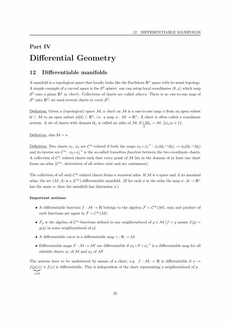
A manifold is a topological space that locally looks like the Euclidean Rn space with its usual topology.A simple example of a curved space is the S2 sphere: one can setup local coordinates (θ, ϕ) which mapS2 onto a plane R2 (a chart). Collections of charts are called atlases. There is no one-to-one map ofS2 onto R2; we need several charts to cover S2.
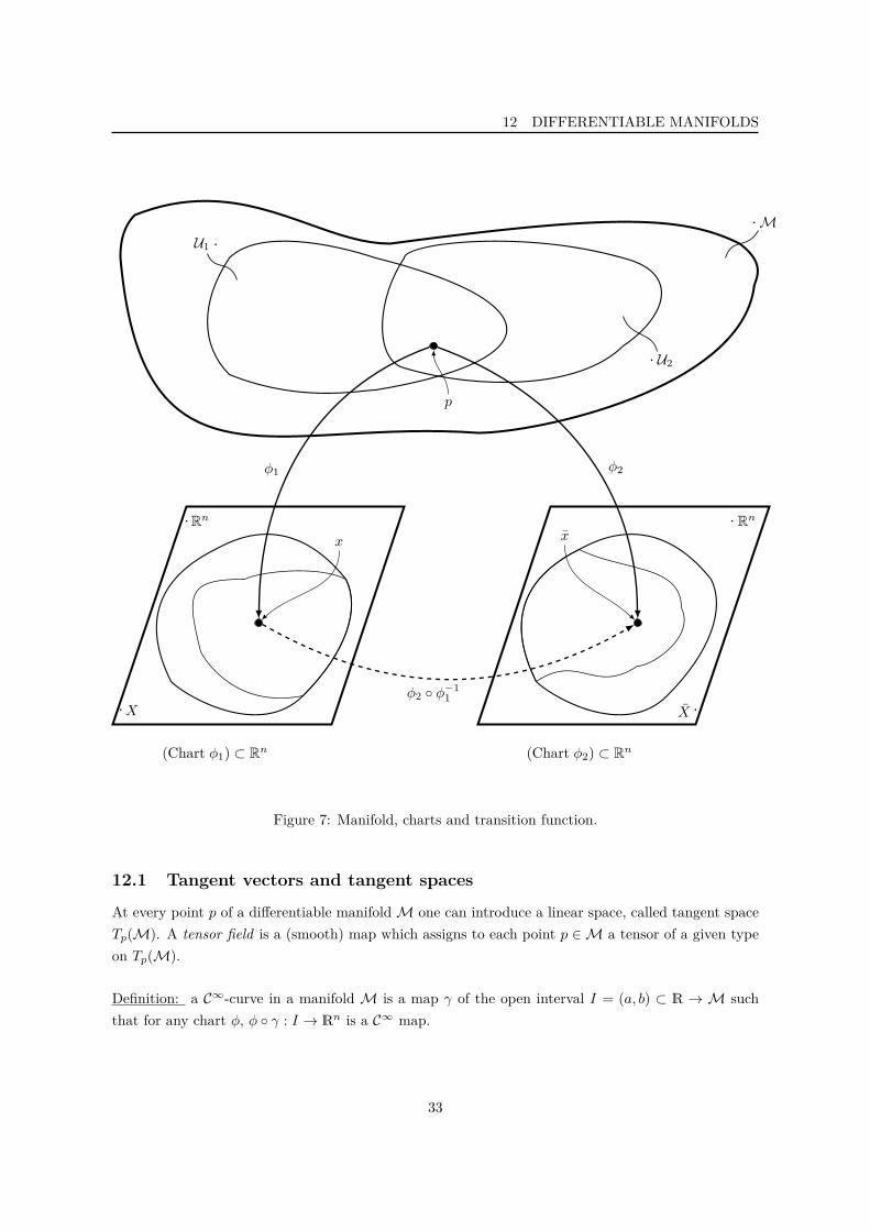
Definition: Given a (topological) spaceM, a chart onM is a one-to-one map φ from an open subsetU ⊂ M to an open subset φ(U) ⊂ Rn, i.e. a map φ : M→ Rn. A chart is often called a coordinatesystem. A set of charts with domain Uα is called an atlas ofM, if
⋃αUα =M, φα|α ∈ I.
Definition: dimM = n
Definition: Two charts φ1, φ2 are C∞-related if both the maps φ2 φ−11 : φ1(U1 ∩ U2) → φ2(U1 ∩ U2)
and its inverse are C∞. φ2 φ−11 is the so-called transition function between the two coordinate charts.
A collection of C∞ related charts such that every point ofM lies in the domain of at least one chartforms an atlas (C∞: derivatives of all orders exist and are continuous).
The collection of all such C∞-related charts forms a maximal atlas. IfM is a space and A its maximalatlas, the set (M, A) is a (C∞)-differentiable manifold. (If for each φ in the atlas the map φ : U → Rn
has the same n, then the manifold has dimension n.)
Important notions:
• A differentiable function f : M → R belongs to the algebra F = C∞(M), sum and product ofsuch functions are again in F = C∞(M).
• Fp is the algebra of C∞-functions defined in any neighbourhood of p ∈ M (f = g means f(q) =g(q) in some neighbourhood of p).
• A differentiable curve is a differentiable map γ : R→M.
• Differentiable maps F :M→M′ are differentiable if φ2 F φ−11 is a differentiable map for all
suitable charts φ1 ofM and φ2 ofM′.
The notions have to be understood by means of a chart, e.g. f : M → R is differentiable if x 7→f(p(x)︸︷︷︸∈M
) ≡ f(x) is differentiable. This is independent of the chart representing a neighbourhood of p.
32
12 DIFFERENTIABLE MANIFOLDS
MU1
U2
Rn
X
Rn
X
p
x x
φ1 φ2
φ2 φ−11
(Chart φ1) ⊂ Rn (Chart φ2) ⊂ Rn
Figure 7: Manifold, charts and transition function.
12.1 Tangent vectors and tangent spaces
At every point p of a differentiable manifoldM one can introduce a linear space, called tangent spaceTp(M). A tensor field is a (smooth) map which assigns to each point p ∈M a tensor of a given typeon Tp(M).
Definition: a C∞-curve in a manifold M is a map γ of the open interval I = (a, b) ⊂ R → M suchthat for any chart φ, φ γ : I → Rn is a C∞ map.
33

12 DIFFERENTIABLE MANIFOLDS
Let f :M→ R be a smooth function onM. Consider the map f γ : I → R, t 7→ f(γ(t)). This hasa well-defined derivative: the rate of change of f along the curve. Consider f φ−1︸ ︷︷ ︸
Rn→Rxi→f(xi)
=f(φ−1(xi))
φ γ︸ ︷︷ ︸I→Rn
t→xi(γ(t))
and
use the chain rule:ddt (f γ) =
n∑i=1
(∂
∂xif(xi)
)dxi(γ(t))
dt . (12.1)
Thus, given a curve γ(t) and a function f , we can obtain a qualitatively new object[
ddt (f γ)
]∣∣∣∣t=t0
,
the rate of change of f along the curve γ(t) at t = t0.
Definition: The tangent vector γp to a curve γ(t) at a point p is a map from the set of real functionsf defined in a neighbourhood of p to R defined by
γp : f 7→[
ddt (f γ)
]p
= (f γ)•p = γp(f). (12.2)
Given a chart φ with coordinates xi, the components of γp with respect to the chart are
(xi γ)•p =[
ddtx
i(γ(t))]p
. (12.3)
The set of tangent vectors at p is the tangent space Tp(M) at p.
Theorem: If the dimension ofM is n, then Tp(M) is a vector space of dimension n (without proof).
We set γ(0) = p (t = 0), Xp = γp, and Xpf = γp(f). Eq. (12.3) determines Xp(xi), the componentsof Xp with respect to a given basis:
Xpf = [f γ]•(0)
=[f φ−1 φ γ
]•(0)
=n∑i=1
∂
∂xi(f φ−1) d
dt (xi γ)(0)
=∑i
(∂
∂xif(x1, . . . , xn)
)(Xp(xi)
).
(12.4)
This way we see that
Xp =∑i
(Xp(xi)
)( ∂
∂xi
)p
, (12.5)
and so the(
∂
∂xi
)p
span Tp(M). From (12.5) we see that Xp(xi) are the components of Xp with
respect to the given basis (Xp(xi) = Xip or Xi).
34

12 DIFFERENTIABLE MANIFOLDS
Suppose that f, g are real functions on M and fg : M → R is defined as fg(p) = f(p)g(p). IfXp ∈ Tp(M), then (Leibniz rule)
Xp(fg) = (Xpf)g(p) + f(p)(Xpg). (12.6)
Notation: (Xf)(p) = Xpf , p ∈M.
Basis of Tp(M): Tp = TP (M) has dimension n. In any basis (e1, . . . , en) we have X = Xiei. Changesof basis are given by
ei = φikek, Xi = φikX
k. (12.7)
The transformations φik and φik are inverse transposed of each other. In particular, ei = ∂∂xi is called
coordinate basis (with respect to a chart). Upon change of chart x 7→ x,
φik = ∂xk
∂xi, φik = ∂xi
∂xk. (12.8)
Definition: The cotangent space T ∗p (or dual space T ∗p of Tp) consists of covectors ω ∈ T ∗p , which arelinear one-forms ω : X 7→ ω(X) ≡< ω,X >∈ R (ω : Tp → R).
In particular for functions f , df : X 7→ Xf is an element of T ∗p . The elements df = f,i dxi =(∂f∂xi
)dxi
form a linear space of dimension n, therefore all of T ∗p .We can define a dual basis (e1, . . . , en) of T ∗p : ω = ωie
i. In particular the dual basis of a basis(e1, . . . , en) of Tp is given by< ei, X >= Xi or< ei, Xjej >= Xj < ei, ej >︸ ︷︷ ︸
δij
= Xi. Thus ωi =< ω, ei >.
Upon changing the basis, the ωi transform like the ei and the ei like the Xi (see (12.7)). In particularwe have for the coordinate basis ei = ∂
∂xi , ei = dxi (< ei, ej >=< dxi, ∂
∂xj >= δij). The change ofbasis is:
∂
∂xi= ∂xk
∂xi∂
∂xk= φi
k ∂
∂xk
dxi = ∂xi
∂xkdxk = φikdxk
(Similar to co- and contravariant vectors.)
Tensors on Tp are multilinear forms on T ∗p and Tp, i.e. a tensor T of type(1
2)(for short T ∈ ⊗1
2Tp):T (ω,X, Y ) is a trilinear form on T ∗p × Tp × Tp. The tensor product is defined between tensors of anytype, i.e. T (ω,X, Y ) = R(ω,X)S(Y ) : T = R⊗ S. In components:
T (ω,X, Y ) = T (ei, ej , ek)︸ ︷︷ ︸≡T ijk
ωiXjY k︸ ︷︷ ︸
ei(ω)ej(X)ek(Y )
, (12.9)
hence T = T ijk ei⊗ ej ⊗ ek. Any tensor of any type can therefore be obtained as a linear combinationof tensor products X ⊗ ω ⊗ ω′ with X ∈ Tp, ω, ω′ ∈ T ∗p . A change of basis can be performed similarly
35
12 DIFFERENTIABLE MANIFOLDS
to the ones for vectors and covectors:
T ijk = Tαβγφiαφj
βφkγ (12.10)
Trace: any bilinear form b ∈ T ∗p ⊗ Tp determines a linear form l ∈ (Tp ⊗ T ∗p )∗ such that l(X ⊗ ω) =b(X,ω). In particular trT is a linear form on tensors T of type
(11), defined by tr(X ⊗ ω) =< ω,X >.
In components with respect to a dual pair of bases we have: trT = Tαα. Similarly T ijk 7→ Sk = T iik
defines for instance a map from tensors of type(1
2)to tensors of type
(01).
12.2 The tangent map
Definition: Let ϕ be a differentiable map: M→ M and let p ∈M, p = ϕ(p). Then ϕ induces a linearmap (“push-forward”):
ϕ∗ : Tp(M)→ Tp(M),
which we can describe in two ways:
(a) For any f ∈ Fp(M) (F : space of all smooth functions onM (or M), that is C∞ map f :M→ R):
(ϕ∗X)f = X(f ϕ)
(b) Let γ be a representative of X (X = γp, see (12.2) and (12.3)). Then let γ = ϕ γ be arepresentative of ϕ∗X. This agrees with (a) since d
dt f(γ(t))∣∣t=0 = d
dt (f ϕ)(γ(t))∣∣t=0.
With respect to bases (e1, . . . , en) of Tp and (e1, . . . , en) of Tp(M), this reads X = ϕ∗X: Xi = (ϕ∗)ikXk
with (ϕ∗)ik =< ei, ϕ∗ek > or in case of coordinate bases: (ϕ∗)ik = ∂xi
∂xk.
Definition: The adjoint map (or “pull-back”) ϕ∗ of ϕ∗ is defined as ϕ∗ : T ∗p → T ∗p , ω 7→ ϕ∗ω (= ω inT ∗p ) with < ϕ∗ω,X >=< ω, ϕ∗X >. The same result is obtained from the definition
ϕ∗ : df 7→ d(f ϕ), f ∈ F(M). (12.10a)
In components, ω = ϕ∗ω reads ωk = ωi(ϕ∗)ik.
Consider (local) diffeomorphisms, i.e. maps ϕ such that ϕ−1 exists in a neighbourhood of p. Note thatdimM = dimM and det
(∂xi
∂xj
)6= 0. Then ϕ∗ and ϕ∗, as defined above, are invertible and may be
extended to tensors of arbitrary types.
Example: tensor of type(1
1)
(ϕ∗T )(ω, X) = T (ϕ∗ω︸︷︷︸ω
, ϕ−1∗ X︸ ︷︷ ︸X
),
(ϕ∗T )(ω,X) = T ((ϕ∗)−1ω︸ ︷︷ ︸ω
, ϕ∗X︸︷︷︸X
).
36

13 VECTOR AND TENSOR FIELDS
Here, ϕ∗ and ϕ∗ are the inverse of each other and we have
ϕ∗(T ⊗ S) = (ϕ∗T )⊗ (ϕ∗S),
tr(ϕ∗T ) = ϕ∗(trT ),(12.11)
and similarly for ϕ∗. In components T = ϕ∗T reads
T ik = Tαβ∂xi
∂xα∂xβ
∂xk(in a coordinate basis). (12.12)
This is formally the same as for transformation (12.10) when changing basis.
13 Vector and tensor fields
Definition: If to every point p of a differentiable manifoldM a tangent vector Xp ∈ Tp(M) is assigned,then we call the map X: p 7→ Xp a vector field onM.
Given a coordinate system xi and associated basis(∂∂xi
)pfor each Tp(M), Xp has components Xi
p withXp = Xi
p
(∂∂xi
)pand Xi
p = Xp(xi) (see (12.5)). Eq. (12.8) shows how Xip transform under coordinate
transformations. The quantity Xf is called the derivative of f with respect to the vector field X. Thefollowing rules apply:
X(f + g) = Xf +Xg,
X(fg) = (Xf)g + f(Xg) (Leibnitz rule).(13.1)
The vector fields onM form a linear space on which the following operations are defined as well:
X 7→ fX (multiplication by f ∈ F),
X, Y 7→ [X,Y ] = XY − Y X (commutator).
[X,Y ], unlike XY , satisfies the Leibniz rule (13.1). The components of the commutator of two vectorfields X, Y relative to a local coordinate basis can be obtained by its action on xi. Thus usingX = Xi ∂
∂xi and Y = Y k ∂∂xk
we get
[X,Y ]j = (XY − Y X)xj
Y xj = Y k∂xj
∂xk= Y kδjk = Y j
XY j = Xk ∂
∂xk(Y j) = Xk Y j ,k︸︷︷︸
∂Y j
∂xk
⇒ XY j − Y Xj = XkY j ,k − Y kXj,k
In a local coordinate basis, the bracket [∂k, ∂j ] clearly vanishes (Xk = 1 and Y k = 1, and thus Y k,j = 0).The Jacobi identity holds:
[X, [Y,Z]] + [Y, [Z,X]] + [Z, [X,Y ]] = 0. (13.2)
37

13 VECTOR AND TENSOR FIELDS
Definition: Let Tp(M)rs be the set of all tensors of rank (r, s) defined on Tp(M) (contravariant of rankr, covariant of rank s). If we assign to every p ∈ M a tensor tp ∈ Tp(M)rs, then the map t : p 7→ tp
defines a tensor field of type(rs
).
Algebraic operations on tensor fields are defined point-wise; for instance the sum of two tensor fieldsis defined by (t+ s)p = tp + sp where t, s ∈ Tp(M)rs. Tensor products and contractions of tensor fieldsare defined analogously. Multiplication by a function f ∈ F(M) is given by (ft)p = f(p)tp. In aneighbourhood U of p, having coordinates (x1, . . . , xn) a tensor field can be expanded in the form
t = ti1...ir j1...js︸ ︷︷ ︸components of t relativeto the coordinate system
(x1, . . . , xn)
(∂
∂xi1⊗ . . .⊗ ∂
∂xir
)⊗(dxj1 ⊗ . . .⊗ dxjs
). (13.3)
If the coordinates are transformed to (x1, . . . , xn) the components of t transform according to
ti1...ir j1...js ≡ tk1...krl1...ls
∂xi1
∂xk1. . .
∂xir
∂xkr∂xl1
∂xj1. . .
∂xls
∂xjs. (13.4)
(We shall consider C∞ tensor fields). Covariant tensors of order 1 are also called one-forms. The setof tensor fields of type
(rs
)is denoted by T rs (M).
Definition: A pseudo-Riemannian metric on a differentiable manifoldM is a tensor field g ∈ T 02 (M)
having the properties:
(i) g(X,Y ) = g(Y,X) for all X,Y
(ii) For every p ∈ M, gp is a non-degenerate (6= 0) bilinear form on Tp(M). This means thatgp(X,Y ) = 0 for all X ∈ Tp(M) if and only if Y = 0.
The tensor field g ∈ T 02 (M) is a (proper) Riemannian metric if gp is positive definite at every point p.
Definition: A (pseudo-)Riemannian manifold is a differentiable manifoldM, together with a (pseudo-)Riemannian metric g.
13.1 Flows and generating vector fields
A flow is a 1-parametric group of diffeomorphisms: ϕt : M → M, s, t ∈ R with ϕt ϕs = ϕt+s. Inparticular ϕ0 = id. Moreover, the orbits (or integral curves) of any point p ∈ M, t 7→ ϕt(p) ≡ γ(t)shall be differentiable. A flow determines a vector field X by means of
Xf = ddt (f ϕt)
∣∣∣∣t=0
(13.5)
i.e. Xp = ddtγ(t)
∣∣t=0 = γ(0) (see (12.2) and (12.3)). γ(0) is the tangent vector to γ at the point
p = γ(0). At the point γ(t) we have then
γ(t) = ddtϕt(p) = d
ds (ϕs ϕt) (p)∣∣∣∣s=0
= Xϕt(p)
38

13 VECTOR AND TENSOR FIELDS
i.e. γ(t) solves the ordinary differential equation:
γ(t) = Xγ(t), γ(0) = p. (13.6)
The generating vector field determines the flow uniquely. Not always does (13.6) admit global solutions(i.e. for all t ∈ R), however for most purposes, “local flows” are good enough.
39

14 LIE DERIVATIVE
14 Lie derivative
The derivative of a vector field V rests on the comparison of Vp and Vp′ at nearby points p, p′. SinceVp ∈ Tp and Vp′ ∈ Tp′ belong to different spaces their difference can be taken only after Vp′ has beentransported to Vp. This can be achieved by means of the tangent map ϕ∗ (Lie transport). The Liederivative LXR of a tensor field R in direction of a vector field X is defined by
LXR = ddtϕ
∗tR
∣∣∣∣t=0
, (14.1)
or more explicitly (LXR)p = ddtϕ
∗tRϕt(p)
∣∣∣∣t=0
. Here ϕt is the (local) flow generated by X, where
ϕ∗tRϕt(p) is a tensor on Tp depending on t.
p
ϕt(p)
Rp
R ϕt(p)
ϕ−t∗ (R ϕt(p)) = ϕ∗t (R ϕt(p))
LXR = ddtϕ
∗tR
∣∣∣∣t=0
= limt→0
1t
(ϕ∗tR−R)
t→ ϕt(p) = γ(t);Xp = ddtγ(t)|t=0 = γ(0)
(ϕ∗ is the inverse of ϕ∗ )
Figure 8: Illustration of the Lie derivative
In order to express LX in components we write ϕt in a chart: ϕt : x 7→ x(t), and linearize it for smallt: xi = xi + tXi(x) +O(t2), xi = xi − tXi(x) +O(t2), thus ∂2xi
∂xk∂t= − ∂2xi
∂xk∂t= Xi
,k at t = 0.As an example, let R be of type
(11). By (12.12) we have (ϕ∗tR)ij(x) = Rαβ(x) ∂x
i
∂xα∂xβ
∂xj . Taking(according to (14.1)) a derivative with respect to t at t = 0 yields
(LXR)ij = Rij,kXk −RαjXi
,α +RiβXβ,j (14.2)
(first term: ∂
∂xkRαβ(x)︸ ︷︷ ︸
Rαβ,k(x)
∂xk
∂t︸︷︷︸Xk
∂xi
∂xα∂xβ
∂xj
∣∣∣∣t=0
= Rij,kXk).
40

14 LIE DERIVATIVE
Properties of LX :
(a) LX is a linear map from tensor fields to tensor fields of the same type.
(b) LX(trT ) = tr(LXT )
(c) LX(T ⊗ S) = (LXT )⊗ S + T ⊗ (LXS)
(d) LXf = Xf (f ∈ F(M))
(e) LXY = [X,Y ] (Y vector field)
(proof: (a) follows from (14.1), (b) and (c) from (12.11), (d) from (13.5), whereas (e) is more involved).
Further properties of LX : if X,Y are vector fields and λ ∈ R, then
(i) LX+Y = LX + LY , LλX = λLX
(ii) L[X,Y ] = [LX , LY ] = LX LY − LY LX
“Proof” of (ii): Apply it to f ∈ F(M),
[LX , LY ]f = LX LY f − LY LXf = LX(Y f)− LY (Xf) = XY f − Y Xf = [X,Y ]f = L[X,Y ]f.
Next apply it on a vector field Z:
[LX , LY ]Z =(e)
[X, [Y,Z]]− [Y, [X,Z]] =Jacobiidentity
[[X,Y ], Z] = L[X,Y ]Z.
For higher rank tensors the derivation follows from the use of (c).If [X,Y ] = 0 then LXLY = LY LX and for φ and ψ, which are the flows generated by X and Y , onefinds: φs ψt = ψt φs.
41

15 DIFFERENTIAL FORMS
15 Differential forms
Definition: A p-form Ω is a totally antisymmetric tensor field of type(0p
)Ω(Xπ(1), . . . , Xπ(p)) = (sign π)Ω(X1, . . . , Xp)
for any permutation π of 1, . . . , p (π ∈ Sp (group of permutations)) with sign π being its parity. Forp > dimM, Ω ≡ 0. Any tensor field of type
(0p
)can be antisymmetrized by means of the operation A:
(AT )(X1, . . . , Xp) = 1p!∑π∈Sp
(sign π)T (Xπ(1), . . . , Xπ(p)) (15.1)
with A2 = A. The exterior product of a p1-form Ω1 with a p2-form Ω2 is the (p1 + p2)-form:
Ω1 ∧ Ω2 = (p1 + p2)!p1! p2! A(Ω1 ⊗ Ω2) (15.2)
Properties:
• Ω1 ∧ Ω2 = (−1)p1p2 Ω2 ∧ Ω1
• Ω1 ∧ (Ω2 ∧ Ω3) = (Ω1 ∧ Ω2) ∧ Ω3 = (p1 + p2 + p3)!p1! p2! p3! A(Ω1 ⊗ Ω2 ⊗ Ω3)
The components in a local basis (e1, . . . , en) of 1-forms are
Ω = Ωi1...ipei1 ⊗ . . .⊗ eip = AΩ
= Ωi1...ipA(ei1 ⊗ . . .⊗ eip)
=n∑
i1=1· · ·
n∑ip=1
Ωi1...ip1p!e
i1 ∧ . . . ∧ eip
=∑
1≤i1<...<ip≤nΩi1...ipei1 ∧ . . . ∧ eip (15.3)
A covariant tensor of rank p, which is antisymmetric under exchange of any pair of indices (i.e. is ap-form), in n dimensions has
(np
)= n!
(n−p)!p! independent components.
Examples:
• For 1-forms A, B (vector fields) we have
(A ∧B)ik = AiBk −AkBi = (−1)(B ∧A)ik.
• For a 2-form A and a 1-form B
(A ∧B)ikl = AikBl +AklBi +AliBk, (15.4)
42
15 DIFFERENTIAL FORMS
since
A ∧B = (1 + 2)!1! 2! A(A⊗B)
= 3!1! 2! (AikBl)
13!e
i ∧ ek ∧ el
= 12(AikBl)ei ∧ ek ∧ el
= 12
13(AikBl + cyclic permutations)ei ∧ ek ∧ el
= (AikBl + cyclic permutations) 13!e
i ∧ ek ∧ el.
Thus by comparing with (15.3) we get (15.4).
15.1 Exterior derivative of a differential form
The derivative df of a 0-form f ∈ F is the 1-form df(X) = Xf : the argument X (vector) acts asa derivation. In a local coordinate basis: df = ∂f
∂xidxi. The exterior derivative is performed by an
operator d applied to forms, converting p-forms to (p + 1)-forms. The derivative dΩ of a 1-form Ω isgiven by
dΩ(X1, X2) = X1Ω(X2)−X2Ω(X1)− Ω([X1, X2]). (15.5)
This expression is verified as follows:
X1Ω(X2) = X1 〈Ω, X2〉︸ ︷︷ ︸1-form
= Xi1∂
∂xi︸︷︷︸,i
(ΩkXk
2)
= Xi1Ωk,iXk
2 +Xi1ΩkXk
2,i,
X2Ω(X1) = Xk2 Ωi,kXi
1 +Xk2 ΩiXi
1,k,
Ω([X1, X2]) = 〈Ω, X1X2 −X2X1〉 = Ωi(X1X2 −X2X1)i = Ωi(Xk
1Xi2,k −Xk
2Xi1,k),
then
dΩ(X1, X2) = (Ωk,i − Ωi,k)Xi1X
k2 .
This is manifestly a 2-form (the coefficient also fits the expectations: 12!
(1+1)!1!1! = 1). One can easily
verify thatdΩ(fX1, X2) = fdΩ(X1, X2). (15.6)
For Ω ∧ f = fΩ (as f is a 0-form), the product rule
d(Ω ∧ f) = dΩ ∧ f − Ω ∧ df
43

15 DIFFERENTIAL FORMS
applies, as one can verify
d(Ω ∧ f)(X1, X2) =(15.5)
X1(fΩ)(X2)−X2(fΩ)(X1)− (fΩ)([X1, X2]),
and
X1(fΩ)(X2) = Xi1∂
∂xi(fΩkXk
2 ) = fXi1∂
∂xi(ΩkXk
2)
︸ ︷︷ ︸fX1Ω(X2)
+Xi1∂f
∂xiΩkXk
2︸ ︷︷ ︸df(X1)Ω(X2)
.
So
d(f ∧ Ω)(X1, X2) = fdΩ(X1, X2)︸ ︷︷ ︸dΩ∧f
+ Ω(X2)df(X1)− Ω(X1)df(X2)︸ ︷︷ ︸−Ω∧df
. (15.7)
Moreover we have d2f = 0, since
d2f(X1, X2) =(15.5)
X1df(X2)−X2df(X1)− df([X1, X2])
= X1X2f −X2X1f − [X1, X2]f = 0.
(15.8)
The generalization of the definition to a p-form Ω gives
dΩ(X1, .. , Xp+1) =p+1∑i=1
(−1)i−1XiΩ(X1, .. , Xi, .. , Xp+1)
+p+1∑i<j
(−1)i+jΩ([Xi, Xj ], X1, .. , Xi, .. , Xj , .. , Xp+1), (15.9)
whereˆmeans omission, e.g. (X1, X2, X3) = (X1, X3).
One can show that the following properties hold:
(a) d is a linear map from p-forms to p+ 1-forms,
(b) d(Ω1 ∧ Ω2) = dΩ1 ∧ Ω2 + (−1)p1Ω1 ∧ dΩ2,
(c) d2 = 0, i.e. d(dΩ) = 0,
(d) df(X) = Xf (f ∈ F),
By means of (a)-(d) we have an alternative definition of d. By eq. (15.3) we have with respect to acoordinate basis
Ω = 1p!Ωi1...ipdxi1 ∧ . . . ∧ dxip , and hence (15.10a)
dΩ =︸︷︷︸ddxip=0
1p!dΩi1...ip ∧ dxi1 ∧ . . . ∧ dxip (15.10b)
44
15 DIFFERENTIAL FORMS
Components:
p! dΩ = Ωi1...ip,i0 dxi0 ∧ dxi1 ∧ . . . ∧ dxip
= −Ωi0i2...ip,i1dxi0 ∧ . . . ∧ dxip
= (−1)kΩi0...ik...ip,ikdxi0 ∧ . . . ∧ dxip (k = 0, . . . , p)
⇒ dΩ = 1p!
1p+ 1︸ ︷︷ ︸
1(p+1)!
p∑k=0
(−1)kΩi0...ik...ip,ik︸ ︷︷ ︸(dΩ)i0...ip
dxi0 ∧ . . . ∧ dxip (15.11)
Examples:
• p = 1:(dΩ)ik = Ωk,i − Ωi,k (15.12)
• p = 2:(dΩ)ikl = Ωik,l + Ωkl,i + Ωli,k (15.13)
Consider a map ϕ :M→ M and ϕ∗ : T ∗p (M)→ T ∗p (M); then
ϕ∗ d = d ϕ∗. (15.14)
A “proof” is found by using (15.10), (12.11) and property (b). It suffices to verify (15.14) on 0-formsand 1-forms. For 0-forms f , (15.14) is identical to (12.10a). For 1-forms which are differentials df ,due to (c) we have
(ϕ∗ d)(df) = 0 (d2f = 0),
(d ϕ∗)(df) = d(ϕ∗ df) =(12.10a)(ϕ∗ df)=d(fϕ)
d(d(f ϕ)) = d2(f ϕ) = 0.
Setting ϕ = ϕt (the flow generated by X) and forming (14.1) (LXR = ddtϕ∗tR∣∣t=0), one obtains the
infinitesimal version of (15.14):LX d = d LX . (15.15)
Definition: A p-form ω with
• ω = dη is exact
• dω = 0 is closed
An exact p-form is always closed (d2η = 0), but the converse is not generally true (Poincaré lemmagives conditions under which the converse is valid).5 6
5η is not unique since gauge transformations η 7→ η + dρ, with ρ any (p− 1)-form, leave dη unchanged.6This is a generalization of the results of three-dimensional vector analysis: rot grad f = 0 and div rot~k = 0.
45

15 DIFFERENTIAL FORMS
The integral of an n-form:
M is orientable within an atlas of “positively oriented” charts, if det(∂xi
∂xj
)> 0 for any change of
coordinates. For an n-form ω (n = dimM):
ω = ωi1...in1n!dx
i1 ∧ . . . ∧ dxin = ω1...n︸ ︷︷ ︸ω(x)
dx1 ∧ . . . ∧ dxn (15.16)
is determined by the single component ω(x); under a change of coordinates ω(x) transforms like
ω(x) = ω1...n = ωi1...in︸ ︷︷ ︸totally
antisymmetric
∂xi1
∂x1 · · ·∂xin
∂xn= ω(x) det
(∂xi
∂xj
). (15.17)
The integral of a n-form is defined as follows:∫M
ω =∫U
dx1 . . . dxn ω(x1, . . . , xn) (if the support of ω is contained in a chart U).
This integral is independent of the choice of coordinates, since in different coordinates∫dx1 . . . dxn ω(x) =
∫dx1 . . . dxn ω(x)
∣∣∣∣det(∂xi
∂xj
)∣∣∣∣ and (15.17) applies. 7 8
15.2 Stokes theorem
Let D be a region in a n dimensional differentiable manifoldM. The boundary ∂D consists of thosep ∈ D whose image x in some chart satisfies e.g. x1 = 0. One can show that ∂D is a closed (n − 1)dimension submanifold of M. If M is orientable then ∂D is also orientable. D shall have a smoothboundary and be such that D is compact. Then for every (n− 1)-form ω we have∫
D
dω =∫∂D
ω (15.18)
15.3 The inner product of a p-form
Definition: Let X be a vector field onM. For any p-form Ω we define the inner product as
(iXΩ)(X1, . . . , Xp−1) ≡ Ω(X,X1, . . . , Xp−1) (15.19)
(and zero if p = 0).
Properties:7Actually, it is often impossible to cover the whole manifold with a single set of coordinates. In the general case it is
necessary to introduce different sets of coordinates in different overlapping patches of the manifold, with the constraintthat in the overlap between the patch with coordinate xi and another patch with coordinate xi, the xi can be expressedin a smooth one-to-one way as functions of xi and vice-versa (orientable manifold).
8The integral over a p-form over the overlap between two patches (xi and xi) can be evaluated using either coordinate
system, provided det(∂xi
∂xj
)> 0.
46

15 DIFFERENTIAL FORMS
(a) iX is a linear map from p-forms to (p− 1)-forms,
(b) iX(Ω1 ∧ Ω2) = (iXΩ1) ∧ Ω2 + (−1)p1Ω1 ∧ (iXΩ2),
(c) iX2 = 0,
(d) iXdf = Xf = 〈df,X〉 with f ∈ F(M),
(e) LX = iX d + d iX .
Proof of (e): for 0-forms f we have
LXf = Xf,
iX df +d iXf=0
= iXdf = Xf,
and for 1-forms df
LXdf =(15.15)
LXd=dLX
d(LXf) = d(Xf),
iX ddf=0
+ d iXdf = d(Xf).
Application: Gauss theorem
Let X be a vector field. Then d(iXη) is an n-form with dim M = n. η is an n-form, and if ηp 6= 0 ∀p ∈M, then η is a “volume form”. A function divηX ∈ F is defined through
(divηX)η = d(iXη) = LXη.9 (15.20)
We can apply Stokes theorem since d(iXη) is an n-form and thus iXη an (n− 1)-form:∫D
d(iXη) =∫D
(divηX)η =∫∂D
iXη. (15.21)
The standard volume form η is given by η =√|g|dx1 ∧ . . . ∧ dxn.
9dη = 0, thus LX = iX d + d iX applied on η gives LXη = iX dη + d(iXη).
47
16 AFFINE CONNECTIONS: COVARIANT DERIVATIVE OF A VECTOR FIELD
Expression for divηX in local coordinates:
Let η = a(x) dx1 ∧ . . . ∧ dxn, X = Xi ∂∂xi . Then since (divηX)η = LXη, we have (using property (c)
of the Lie derivative):
LXη = (Xa) dx1 ∧ . . . ∧ dxn + a
n∑i=1
dx1 ∧ . . . ∧ d(Xxi) ∧ . . . ∧ dxn.
Since d(Xxi) = d(Xk ∂
∂xkxi︸ ︷︷ ︸
δik
) = dXi(x) = Xi,jdxj , but dx1 ∧ . . . ∧ dxj ∧ . . . ∧ dxn 6= 0 only if j = i
(otherwise we have two identical dxi) we find
LXη = Xa︸︷︷︸Xi ∂a
∂xi
dx1 ∧ . . . ∧ dxn + a
n∑i=1
Xi,idx1 ∧ . . . ∧ dxn
= (Xia,i + aXi,i)
1aη
⇒ divηX = 1a
(aXi),i = 1√|g|
(√|g|Xi
),i
for the “standard” η. (15.22)
16 Affine connections: Covariant derivative of a vector field
Definition: An affine (linear) connection or covariant differentiation on a manifold M is a mapping∇ which assigns to every pair X,Y of C∞ vector fields onM another C∞ vector field ∇XY with thefollowing properties:
(i) ∇XY is bilinear in X and Y ,
(ii) if f ∈ F(M), then
∇fXY = f∇XY,
∇X(fY ) = f∇XY +X(f)Y.
(16.1)
Lemma: Let X and Y be vector fields. If X vanishes at the point p onM, then ∇XY also vanishes atp.
Proof: Let U be a coordinate neighbourhood of p. On U we have the representation X = ξi ∂∂xi ,
ξi ∈ F(U) with ξi(p) = 0. Then (∇XY )p = ∇ξi ∂
∂xiY = ξi(p)︸ ︷︷ ︸
=0
[∇ ∂
∂xiY ]p = 0.
Since ∇XY produces again a vector field, the result of the covariant differentiation can only be a linearcombination of again the basis in the current chart. This leads us to the following statement:
48

16 AFFINE CONNECTIONS: COVARIANT DERIVATIVE OF A VECTOR FIELD
Definition: One sets, relative to a chart (X1, . . . , Xn) for U ⊂M:
∇ ∂
∂xi
(∂
∂xj
)= Γkij
∂
∂xk(16.2)
The n3 functions Γkij ∈ F(U) are called Christoffel symbols (or connection coefficients) of the connection∇ in a given chart.10
The Christoffel symbols are not tensors:
∇ ∂∂xa
(∂
∂xb
)= Γcab
∂
∂xc= Γcab
∂xk
∂xc∂
∂xk. (16.3)
If we use (16.1):
∇ ∂∂xa
(∂
∂xb
)= ∇( ∂xi
∂xa∂
∂xi
) (∂xj∂xb
∂
∂xj
)= ∂xi
∂xa
[∂xj
∂xbΓkij
∂
∂xk+ ∂
∂xi
(∂xj
∂xb
)∂
∂xj
]
= ∂xi
∂xa∂xj
∂xbΓkij
∂
∂xk+ ∂2xj
∂xa∂xb∂
∂xj.
Comparison with 16.3:
∂xk
∂xcΓcab = ∂xi
∂xa∂xj
∂xbΓkij + ∂2xk
∂xa∂xb
⇒ Γcab = ∂xi
∂xa∂xj
∂xb∂xc
∂xkΓkij + ∂xc
∂xk∂2xk
∂xa∂xb(16.4)
The second term is not compatible with being a tensor.If for every chart there exist n3 functions Γkij which transform according to (16.4) under a change
of coordinates, then one can show that there exists a unique affine connection ∇ onM which satisfies(16.3).
Definition: for every vector field X we can introduce the tensor ∇X ∈ T 11 (M) defined by
∇X(Y, ω) ≡ 〈ω,∇YX〉 , (16.5)
where ω is a one-form. ∇X is called the covariant derivative of X.
In a chart (x1, . . . , xn), let X = ξi∂i and ∇X = ξi;jdxj ⊗ ∂i (< dxi, ∂i >= δik):
ξi;j = ∇X(∂j ,dxi) =⟨dxi,∇∂jX
⟩=⟨dxi, ξk,j∂k + ξkΓδjk∂δ
⟩= ξi,j + Γijkξk 11 (16.6)
10For a pseudo-Riemannian manifold, the corresponding connection coefficients are given by (9.6) or (9.11).11semicolon shall denote the covariant derivative (”normal derivative” + additional terms, that vanish in (cartesian)
Euclidean or Minkowski space)
49

16 AFFINE CONNECTIONS: COVARIANT DERIVATIVE OF A VECTOR FIELD
16.1 Parallel transport along a curve
Definition: let γ : I →M be a curve inM with velocity field γ(t), and let X be a vector field on someopen neighbourhood of γ(I). X is said to be autoparallel along γ if
∇γX = 0. (16.7)
The vector ∇γX is sometimes denoted as DXdt or ∇Xdt (covariant derivative along γ). In terms of
coordinates, we have X = ξi∂i, γ = dxidt ∂i (see (12.3)). With (16.1) and (16.2) we get
∇γX = ∇ dxidt ∂i
(ξk∂k)
= dxi
dt ∇∂i(ξk∂k)
= dxi
dt
[ξkΓjik∂j + ∂iξ
k∂k
]= dxi
dt[ξjΓkij∂k + ∂iξ
k∂k]
=[
dξk
dt + Γkijdxi
dt ξj
]∂k, (16.8)
where we used dxi
dt∂ξk
∂xi= dξk
dt . This shows that ∇γX only depends on the values of X along γ. Interms of coordinates we get for (16.7)
dξk
dt + Γkijdxi
dt ξj = 0. (16.9)
For a curve γ and any two point γ(s) and γ(t) consider the mapping
τt,s : Tγ(s)(M)→ Tγ(t)(M),
which transforms a vector v(s) at γ(s) into the parallel transported vector v(t) at γ(t). The mappingτt,s is the parallel transport along γ from γ(s) to γ(t). We have τs,s = 1 and τr,s τs,t = τr,t.
We can now give a geometrical interpretation of the covariant derivative that will be generalizedto tensors. Let X be a vector field along γ, then
∇γX(γ(t)) = dds
∣∣∣∣s=t
τt,sX(γ(s)), (16.10)
Proof: Let’s work in a given chart. By construction, v(t) = τt,sv(s) with v(s) ∈ Tγ(s)(M) and due to(16.8) it satisifies: vi + Γikj xkvj = 0. If we write (τt,sv(s))i = (τt,s)ijv
j(s) = vi(t) (with τt,s = (τs,t)−1
50

16 AFFINE CONNECTIONS: COVARIANT DERIVATIVE OF A VECTOR FIELD
M
γ(s)
γ(t)γ
v(s)
v(t)τt,s
Figure 9: Illustration of parallel transport.
and τs,s = 1), we get
vi(s) = ddt
∣∣∣∣t=s
vi(t)
= ddt
∣∣∣∣t=s
[(τt,s)ijv
j(s)]
=(
ddt
∣∣∣∣t=s
(τt,s)ij
)vj(s)
= −Γikj xkvj(s).
⇒ ddt
∣∣∣∣t=s
(τt,s)ij = −Γikj xk (16.11)
Since τt,s = (τs,t)−1, dds∣∣s=t (τt,s)ij = − d
dt∣∣t=s (τt,s)ij = Γikj xk. Then
dds
∣∣∣∣s=t
[τt,sX(γ(s))]i =(
dds
∣∣∣∣s=t
τt,s
)ij
Xj + dds
∣∣∣∣s=t
Xi(γ(s))
= Γikj xkXj +Xi,j
dxj(γ(s))ds
∣∣∣∣s=t
,
which is again (16.8) (X = ξi∂i and the second term gives dξidt ).
51

16 AFFINE CONNECTIONS: COVARIANT DERIVATIVE OF A VECTOR FIELD
Definition: If ∇XY = 0, then Y is said to be parallel transported with respect to X.
Geometrical interpretation of parallel transport: Consider the differential dAi = Ai,jdxj = Ai(x +dx)− Ai(x). In order that the difference of two vectors be a vector, we have to consider them at thesame position. The transport has to be chosen such that for cartesian coordinates there is no changein transporting it. The covariant derivative exactly achieves this.
Definition: Let X be a vector field such that ∇XX = 0. Then the integral curves of X are calledgeodesics.
In local coordinates xi the curve is given by (using (12.3) and (13.6)) the requirement ddtx
i(t) =Xi(x(t)). Inserting this into (16.8) and using d2xi
dt2 = dXidt , we get
xk + Γkij xixj = 0. (16.12)
For a vector parallel transported along a geodesic, its length and angle with the geodesic does notchange.
16.2 Round trips by parallel transport
Consider (16.8) and denote ξi = vi, thus
vi = −Γikj xkvj . (16.13)
Let γ : [0, 1]→M be a closed path, wih γ(0) = p = γ(1). Displace a vector v0 ∈ Tp(M) parallel alongγ and obtain the field v(t) = τt,0v0 ∈ Tγ(t)(M). We assume that the closed path is sufficiently small(such that we can work in the image of some chart), thus we can expand Γikj(x) around the pointx(0) = x0 on the curve:
Γikj(x) ' Γikj(x0) + (xρ − xρ0) ∂
∂xρΓikj(x)
∣∣∣∣x=x0
+ · · · (16.14)
Thus (16.13) is to first order in (xk − xk0):
t∫0
vi dt = vi(t)− vi0 = −t∫
0
Γikj vj︸︷︷︸'vj0
xk dt ≈ −Γikj(x0)vj0
t∫0
xk dt
︸ ︷︷ ︸xk(t)−xk0
,
taking only the first term in the expansion of Γ. And hence,
vi(t) = vi0 − Γikj(x0)(xk(t)− xk0)vj0 + · · · (16.15)
52
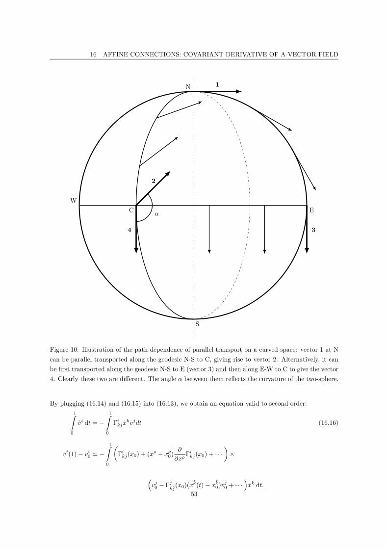
16 AFFINE CONNECTIONS: COVARIANT DERIVATIVE OF A VECTOR FIELD
N
E
S
WC
1
2
34
α
Figure 10: Illustration of the path dependence of parallel transport on a curved space: vector 1 at Ncan be parallel transported along the geodesic N-S to C, giving rise to vector 2. Alternatively, it canbe first transported along the geodesic N-S to E (vector 3) and then along E-W to C to give the vector4. Clearly these two are different. The angle α between them reflects the curvature of the two-sphere.
By plugging (16.14) and (16.15) into (16.13), we obtain an equation valid to second order:1∫
0
vi dt = −1∫
0
Γikj xkvjdt (16.16)
vi(1)− vi0 ' −1∫
0
(Γikj(x0) + (xρ − xρ0) ∂
∂xρΓikj(x0) + · · ·
)×
(vj0 − Γj
kj(x0)(xk(t)− xk0)vj0 + · · ·
)xk dt.
53

16 AFFINE CONNECTIONS: COVARIANT DERIVATIVE OF A VECTOR FIELD
Multiplying out and discarding terms of third order or higher in xk − xk0 , we get:
vi(1) ' vi0 − Γikj(x0)vj0
1∫0
xk dt
︸ ︷︷ ︸xk(1)−xk(0)
=0
−[∂
∂xρΓikj(x0)− Γi
kj(x0)Γjρj(x0)
]vj0
1∫0
(xρ − xρ0)xk dt.
Since we are considering a closed path (∫ 1
0 x dt = xk(1)− xk(0) = 0),
∆vi = vi(1)− vi(0) = −[∂
∂xρΓikj(x0)− Γikl(x0)Γlρj(x0)
]vj0
1∫0
xρxk dt,
with
1∮0
xρxk dt =1∮
0
ddt (x
ρxk) dt
︸ ︷︷ ︸=0
−1∮
0
xρxk dt = −1∮
0
xρxk dt,
antisymmetric in (ρ, k). Then
∆vi = −12
[∂
∂xρΓikj − ΓiklΓlρj −
∂
∂xkΓiρj + ΓiρlΓlkj
](x0)︸ ︷︷ ︸
−Rijkρ
vj0
1∫0
xρxk dt,
∆vi = 12R
ijkρ(x0)vj0
1∫0
xρxk dt. (16.17)
We shall see that Rijkρ is the curvature tensor.
Rijkρ = ∂
∂xkΓiρj −
∂
∂xρΓikj + ΓlρjΓikl − ΓlkjΓiρl (16.18)
Thus an arbitrary vector vi will not change when parallel transported around an arbitrary small closedcurve at x0 if and only if Rijkρ vanishes at x0.
16.3 Covariant derivatives of tensor fields
The parallel transport is extended to tensors by means of the requirements:
τs,t(T ⊗ S) = (τs,tT )⊗ (τs,tS),
τs,t tr(T ) = tr(τs,tT ),
τs,t c = c (c ∈ R).
54

16 AFFINE CONNECTIONS: COVARIANT DERIVATIVE OF A VECTOR FIELD
For e.g. a covariant vector ω, 〈τs,t ω, τs,tX〉γ(s) = 〈ω,X〉γ(t) and for a tensor of type(1
1): τs,t T (τs,t ω, τs,tX) =
T (ω,X). In components:(τs,tT )ik = Tαβ(τs,t)iα(τs,t)kβ (16.19)
(τik is inverse transpose of τ ik). The covariant derivative ∇X (X vector field, T tensor field) associatedto τ is
(∇XT )p = ddt τ0,tTγ(t)
∣∣∣∣t=0
, (16.20)
with γ(t) any curve with γ(0) = p and γ(0) = Xp (generalization of (16.10)).
Properties of the covariant derivative:
(a) ∇X is a linear map from tensor fields to tensor fields of the same type(rr
),
(b) ∇Xf = Xf ,
(c) ∇X(trT ) = tr(∇XT ),
(d) ∇X(T ⊗ S) = (∇XT )⊗ S + T ⊗ (∇XS).
This follows from the properties of τs,t. For a 1-form ω we have:
(∇Xω)(Y ) = tr(∇Xω ⊗ Y )
= tr(∇X(ω ⊗ Y ))− tr(ω ⊗∇XY )
= ∇X tr(ω ⊗ Y )− ω(∇XY )
= Xω(Y )− ω(∇XY ). (16.21)
General differentiation rule for a tensor field of type(1
1):
(∇XT )(ω, Y ) = XT (ω, Y )− T (∇Xω, Y )− T (ω,∇XY ) (16.22)
Due to (a)-(d), the operation ∇X is completely determined by its action on vector fields Y , which arethe affine connections (see (16.1) and (16.2)).
16.4 Local coordinate expressions for covariant derivative
Let T ∈ T qp (U) be a tensor of rank (p, q) with local coordinates (x1, . . . , xn) valid in a region U . Wehave T i1...ip j1...jq ∂i1 ⊗ . . .⊗ ∂ip ⊗ dxj1 ⊗ . . .⊗ dxjq and X = Xk∂k. Let us use
XT i1...ip j1...jq = XkT i1...ip j1...jq,k (16.23)
and write (16.2):∇X(∂i) = Xk∇∂k∂i = XkΓlki∂l . (16.24)
55
16 AFFINE CONNECTIONS: COVARIANT DERIVATIVE OF A VECTOR FIELD
Moreover,
(∇Xdxj)(∂i)(16.21)= X
⟨dxj , ∂i
⟩︸ ︷︷ ︸δji︸ ︷︷ ︸0
−⟨dxj ,∇X∂i
⟩
= −XkΓjki ,
or ∇Xdxj = −XkΓjkidxi. (16.25)
Using (16.23), (16.24) and (16.25) for ωj = dxj , Yi = ∂i we obtain the following expression for ∇XT :
T i1...ip j1...jq ;k = T i1...ip j1...jq,k + Γi1kl Tli2...ip
j1...jq + . . .+ Γipkl Ti1...ip−1l
j1...jq
− Γlkj1 Ti1...ip
lj2...jq − . . .− Γlkjq Ti1...ip
j1...jq−1l. (16.26)
Examples:
• Contravariant and covariant vector fields:
ξi;k = ξi,k + Γiklξl,
ηi;k = ηi,k − Γlkiηl,
• Kronecker tensor:δij;k = 0,
• Tensor(1
1):
T ik;r = T ik,r + ΓirlT lk − ΓlrkT il.
The covariant derivative of a tensor is again a tensor. Consider the covariant derivative of the metricgµν :
gµν;λ = ∂gµν∂xλ
− Γρλµgρν − Γρλνgρµ. (16.27)
Inserting into this the expressions of Γρλµ given by (9.11) leads us to
gµν;λ = 0. (16.28)
This is not surprising since gµν;λ vanishes in locally inertial coordinates and being a tensor it is thenzero in all systems.
Covariance principle: Write the appropriate special relativistic equations that hold in the absence ofgravitation, replace ηαβ by gαβ , and replace all derivatives with covariant derivatives (, → ;). The resultingequations will be generally covariant and true in the presence of gravitational fields.
56

17 CURVATURE AND TORSION OF AN AFFINE CONNECTION, BIANCHI IDENTITIES
17 Curvature and torsion of an affine connection, Bianchi iden-tities
Let an affine connection be given onM, let X, Y , Z be vector fields.
Definition:
T (X,Y ) = ∇XY −∇YX − [X,Y ] (17.1)
R(X,Y ) = ∇X∇Y −∇Y∇X −∇[X,Y ] (17.2)
T (X,Y ) is antisymmetric and f -linear in X, Y and then defines a tensor of type(1
2)through:
(ω,X, Y )→ 〈ω, T (X,Y )〉 is thus a(1
2)tensor field called the torsion tensor.
f -linearity:T (fX, gY ) = fgT (X,Y ) f, g,∈ F(M).
In local coordinates, the components of the torsion tensor are given by:
T kij =⟨dxk, T (∂i, ∂j)
⟩=⟨
dxk,∇∂i∂j︸ ︷︷ ︸=Γl
ij∂l
−∇∂j∂i − [∂i, ∂j ]︸ ︷︷ ︸=0
⟩
= Γkij − Γkji (17.3)
(using that⟨dxk, ∂l
⟩= δkl). In particular, we have T kij = 0⇔ Γkij = Γkji.
R(X,Y ) = −R(Y,X) is antisymmetric in X,Y . The vector field R(X,Y )Z is f -linear in X, Y , Z:(R(fX, gY )hZ = fghR(X,Y )Z; f, g, h ∈ F(M)). R determines a tensor of type
(13): the Riemann
tensor or curvature tensor.
(ω,Z,X, Y )→ 〈ω,R(X,Y )Z〉 ≡ RijklωiZjXkY l
In components with respect to local coordinates:
Rijkl =⟨dxi, R(∂k, ∂l)∂j
⟩=⟨dxi, (∇∂k∇∂l −∇∂l∇∂k)∂j
⟩ 12=⟨dxi,∇∂k(Γslj∂s)−∇∂l(Γskj∂s)
⟩= Γilj,k − Γikj,l + ΓsljΓiks − ΓskjΓils. (17.4)
12Notice that ∇[∂k, ∂l]︸ ︷︷ ︸=0
∂j = 0.
57
17 CURVATURE AND TORSION OF AN AFFINE CONNECTION, BIANCHI IDENTITIES
Eq. (17.4) is exactly the the same as defined in (16.18). It is antisymmetric in the last two indices:Rijkl = −Rijlk.
Definition: The Ricci tensor is the following contraction of the curvature tensor:
Rjl ≡ Rijil = Γilj,i − Γiij,l + ΓsljΓiis − ΓsijΓils (17.5)
The scalar curvature is the trace of the Ricci tensor:
R ≡ gljRjl = Rll (17.6)
Example: For a pseudo-Riemannian manifold the connection coefficients are given by (9.11). Considera two-sphere (which is a pseudo Riemannian manifold) with the metric ds2 = a2(dθ2 + sin2 θdφ2),then:
gθφ = a2
(1 00 sin2 θ
), gθφ = 1
a2
(1 00 1
sin2 θ
).
The non-zero Γ are:
Γθφφ = − sin θ cos θ,
Γφθφ = Γφφθ = cot θ.
The Riemann tensor is given by
Rθφθφ = ∂θΓθφφ − ∂φΓθθφ + ΓθθλΓλφθ − ΓθφλΓλθφ
= (sin2 θ − cos2 θ)− 0 + 0− (− sin θ cos θ) cot θ
= sin2 θ.
The Ricci tensor has the following components:
Rφφ = Rθφθφ +Rφφφφ︸ ︷︷ ︸=0
= sin2 θ,
Rθθ = 1,
Rθφ = Rφθ = 0.
The Ricci scalar is
R = gθθ︸︷︷︸1a2
Rθθ︸︷︷︸1
+ gφφ︸︷︷︸1
a2 sin2 θ
Rφφ︸︷︷︸sin2 θ
+gθφ Rθφ︸︷︷︸0
+gφθ Rφθ︸︷︷︸0
= 1a2 + 1
a2 sin2 θsin2 θ
= 2a2 .
58

17 CURVATURE AND TORSION OF AN AFFINE CONNECTION, BIANCHI IDENTITIES
The Ricci scalar is constant over this two-sphere and positive, thus the sphere is “positively curved”.13 14 15
17.1 Bianchi identities for the special case of zero torsion
X, Y and Z are vector fields, then
R(X,Y )Z + cyclic = 0 (1st Bianchi identity), (17.7)
(∇XR)(Y,Z) + cyclic = 0 (2nd Bianchi identity). (17.8)
Proof of the 1st identity: Torsion = 0⇒ ∇XY −∇YX = [X,Y ]. Then
(∇X∇Y −∇Y∇X)Z + (∇Z∇X −∇X∇Z)Y
+ (∇Y∇Z −∇Z∇Y )X −∇[X,Y ]Z −∇[Z,X]Y −∇[Y,Z]X
= ∇X(∇Y Z −∇ZY )−∇[Y,Z]X + cyclic
= [X, [Y,Z]] + cyclic
= 0 due to the Jacobi identity (13.2).
(See textbooks for proof of the 2nd Bianchi identity.)
13For a position independent metric (e.g. Cartesian coordinates) the Riemann tensor (and thus the scalar curvature)vanishes as the Γ vanish.
14For a plane with polar coordinates we get a position dependent metric(
1 00 r2
): ds2 = dr2 + r2dθ2 and thus the
Γ do not vanish. However the curvature vanishes.15The curvature does not depend on the choice of coordinates.
59

18 RIEMANNIAN CONNECTIONS
18 Riemannian connections
Metric: Let M be equipped with a pseudo-Riemannian metric: a symmetric, non-degenerate tensorfield: g(X,Y ) = 〈X,Y 〉 of type
(02).
• Non-degenerate means that, for any point p ∈ M, X,Y ∈ Tp, one has gp(X,Y ) = 0 ∀Y ∈ Tp ⇒X = 0.
• In components, 〈X,Y 〉 = gikXiY k, gik = gki (symmetric) and det gik 6= 0.
• With the metric we can lower and raise indices:
Xi = gikXk, ωi = gikωk,
where gik denotes the inverse of gik. It also works for tensor fields of different types: T ik =Tlkg
il = T ilglk.
• Given a basis (e1, . . . , en) of Tp, the covectors of the dual basis (e1, . . . , en) become themselvesvectors; indeed ei = gije
j .
Riemann connection: The metric tensor g at a point p in M is a symmetric(0
2)tensor. It assigns a
magnitude√|g(X,X)| to each vector X on Tp(M), denoted by d(X) and defines the angle between
any two vectors X, Y ( 6= 0) on Tp(M) via
a(X,Y ) = arccos(
g(X,Y )d(X)d(Y )
). (18.1)
If a(X,Y ) = π2 then X and Y are orthogonal. Further observations:
• The length of a curve with tangent vector X between t1 and t2 is L(t1, t2) =t2∫t1
d(X) dt.
• If (ea) is a basis of Tp(M), the components of g with respect to this basis are gab = g(ea, eb).
• Like in special relativity we classify vectors at a point as timelike (g(X,X) > 0), null (g(X,X) =0) and space like (g(X,X) < 0).
Definition: let (M, g) be a pseudo-Riemannian manifold. An affine connection is a metric connectionif parallel transport along any smooth curve γ onM preserve the inner product: for autoparallel fieldsX(t), Y (t) (see (16.7)), gγ(t)(X(t), Y (t)) is independent of t along γ.
Theorem: an affine connection ∇ is metric if and only if (no proof)
∇g = 0. (18.2)
Eq. (18.2) is equivalent for (g(Y, Z)) to
∇Xg = 0 = Xg(Y, Z)− g(∇XY, Z)− g(Y,∇XZ)
60

18 RIEMANNIAN CONNECTIONS
or
Xg(Y, Z) = g(∇XY,Z) + g(Y,∇XZ). (18.3)
Theorem: For every pseudo-Riemannian manifold (M, g), there exists a unique affine connection suchthat
(a) ∇ has vanishing torsion (∇ is symmetric),
(b) ∇ is metric.
Proof: T = 0 (vanishing torsion) means ∇XY = ∇YX + [X,Y ]. Inserting this into (18.3) (and thelinearity of g) gives
Xg(Y,Z) = g(∇YX,Z) + g([X,Y ], Z) + g(Y,∇XZ). (18.4)
By cyclic permutations one obtains as well
Y g(Z,X) = g(∇ZY,X) + g([Y,Z], X) + g(Z,∇YX), (18.5)
Zg(X,Y ) = g(∇XZ, Y ) + g([Z,X], Y ) + g(X,∇ZY ). (18.6)
Taking the linear combination (18.5) + (18.6) - (18.4), we get (Koszul formula):
2g(∇ZY,X) = −Xg(Y, Z) + Y g(Z,X) + Zg(X,Y )
−g([Z,X], Y )− g([Y, Z], X) + g([X,Y ], Z).
(18.7)
The right hand side is independent of ∇. Since g is non-degenerate, the uniqueness of ∇ follows from(18.7).
Definition: the unique connection on (M, g) from the above theorem is called the Riemannian orLevi-Civita connection.
We determine the Christoffel symbols for the Riemannian connection in a given chart (U , x1, . . . , xn).For this purpose we take X = ∂k, Y = ∂j , Z = ∂i in (18.7) and we use [∂i, ∂j ] = 0 as well as〈∂i, ∂j〉 = gij . The result is
〈∇∂i∂j , ∂k〉 = Γlij 〈∂l, ∂k〉︸ ︷︷ ︸glk
,
2Γlijglk = −∂k 〈∂i, ∂j〉︸ ︷︷ ︸gij
+∂j 〈∂i, ∂k〉︸ ︷︷ ︸gik
+∂i 〈∂k, ∂j〉︸ ︷︷ ︸gkj
,
61

18 RIEMANNIAN CONNECTIONS
or
glkΓlij = 12(gkj,i + gik,j − gji,k). (18.8)
gij denoting the inverse matrix of gij , we obtain
Γlij = 12g
lk(gkj,i + gik,j − gji,k), (18.9)
which is exactly equation (9.11).
Properties of the Riemannian connection:
(i) The inner product of any two vectors remains constant upon parallel transporting them alongany curve γ (g(X,Y )γ(t) = g(X,Y )γ(0)).
(ii) The covariant derivative commutes with raising or lowering indices, e.g. T ik;l = (gkmT im);l
= gkmTim
;l, because gkm;l = 0.
Riemann tensor: the curvature tensor of a Riemannian connection has the following additional sym-metry properties (without proof):
〈R(X,Y )Z,U〉 = −〈R(X,Y )U,Z〉 , (18.10)
〈R(X,Y )Z,U〉 = 〈R(Z,U)X,Y 〉 . (18.11)
In coordinate expression the Riemann tensor satisfies the following symmetries:
Rijkl = −Rijlk is always the case, (18.12)∑(jkl)
Rijkl = 0 1st Bianchi identity, (18.13)
∑(klm)
Rijkl;m = 0 2nd Bianchi identity. (18.14)
Eqs. (18.13) and (18.14) are valid for vanishing torsion. Here∑
(jkl)denotes the cyclic sum. Additionally,
Rijkl = −Rjikl, (18.15)
Rijkl = Rklij , (18.16)
for the Riemannian connection with Rijkl = gisRsjkl.
Ricci and Einstein tensor
62

18 RIEMANNIAN CONNECTIONS
Rik = Rjijk Ricci tensor (18.17)
R = Rii scalar curvature (18.18)
Gik = Rik −12Rgik Einstein tensor (18.19)
By symmetry, Rik = Rki, Gik = Gki and
Rki;k = 12R;i, (18.20)
Gki;k = 0, (18.21)
which are the contracted 2nd Bianchi identity.
Proof: Rik = gjlRlijk = gjlRjkli, 2nd Bianchi identity gives:
Rijkl;m +Rijlm;k +Rijmk;l = 0.
Then we take the (ik)-trace:
Rjl;m + Rijlm;i︸ ︷︷ ︸−gikRjklm;i
−Rjm;l = 0,
Rj l;m − gikRjklm;i −Rjm;l = 0,
(jm)-trace:
Rj l;j + gikRkl;i︸ ︷︷ ︸2Rjl;j
−R;l = 0.
⇒ (18.20)
For (18.21):
Gki = Rki −12g
kiR = Rki −
12δ
kiR
Gki;k = Rki;k −12(δkiR);k = 1
2R;i︸ ︷︷ ︸(18.20)
−12R;i = 0
Without proof in n dimensions, the Riemann tensor has cn = n2(n2−1)12 independent components
(c1 = 0, c2 = 1, c3 = 6, c4 = 20).
63
19 PHYSICAL LAWS WITH GRAVITATION
Part V
General Relativity19 Physical laws with gravitation
19.1 Mechanics
The physical laws are relations among tensors (scalars and vectors being tensors of rank 0 and 1respectively). Thus the physical laws read the same in all coordinate systems (provided the physicalquantities are transformed suitably) and satisfy general covariance (same form). Practically, this meansthat from the special relativity laws that hold in absence of gravitation, we have to replace ηαβ by gαβand replace derivation by covariant derivation.
In an inertial system, we have the equation of motion (see (4.3))
mduα
dτ = fα. (19.1)
According to the equivalence principle, (19.1) holds in a local IS. fα does not contain gravitationalforces as they would vanish in a local IS. We transform it to general KS (coordinate system), then theLorentz vector fα gets transformed to fµ = ∂xµ
∂ξα fα (ξα is in local IS, xµ is in KS). Equation (19.1)
holds in a local IS reads thenm
Duµ
dτ︸ ︷︷ ︸covariant derivative
given in (16.8)
= fµ, (19.2)
(∇X → Ddτ ) with ξ
µ → uµ (dt→ dτ and dxidτ = ui) and thus
Duµ
dτ = duµ
dτ + Γµνλuνuλ.
Then equation (19.2) readsm
duµ
dτ = fµ −mΓµνλuνuλ. (19.3)
We see that on the right hand side there are now gravitational forces appearing explicitly (via Γµνλ).Equation (19.3) (or (19.2)) is covariant (it has the same form in all coordinate systems) and reduces forgµν → ηαβ (thus Γµνλ = 0) to equation (19.1) (in a local IS). The components of uµ are not independentbut satisfy the condition gµνuµuν = c2.
19.2 Electrodynamics
According to the equivalence principle, Maxwell’s equations (see (6.4) and (6.5))
∂αFαβ = 4π
cjβ and εαβγδ∂βFγδ = 0
are valid in a local IS. Applying the covariance principle, they become as follows in a general KS:
Fµν ;ν = 4πcjµ and εµνλκFλκ;ν = 0, (19.4)
64

19 PHYSICAL LAWS WITH GRAVITATION
provided that going from coordinates ξα in a local IS to the KS coordinates xµ we have
jα → jµ = ∂xµ
∂ξαjα and Fµν = ∂xµ
∂ξα∂xν
∂ξβFαβ .
Gravity enters via the Γµνλ in the covariant derivative. The continuity equation ∂αjα = 0 translatesto jµ;µ = 0. It can be shown that in the homogeneous equation the terms with Γ vanish. Thus thecovariant derivative reduces to the ordinary derivative (,) 16.
19.3 Energy-momentum tensor
For an ideal fluid, given by (in a local IS)
Tµν =(ρ+ p
c2
)uµuν − ηµνp, (19.8)
with
• uµ: four-velocity,
• ρ: proper energy density,
• p: pressure of the fluid.
In a KS this becomesTµν =
(ρ+ p
c2
)uµuν − gµνp. (19.9)
In the IS the conservation law implies Tµν,ν = 0 and in the KS Tµν ;ν = 0 (explicitely, Tµν ;ν =Tµν,ν + ΓµνλT νλ + ΓννλTµλ = 0). With (19.5), Γννλ = 1√
g
∂√g
∂xλ, we get instead
Tµν ;ν = 1√g
∂√gTµν
∂xν+ ΓµνλT
νλ = 0. (19.10)
This is no longer a conservation law, as we cannot form any constant of motion from (19.10). Thisshould also not be expected, since the system under consideration can exchange energy and momentumwith the gravitational field.
16g = det(gik) = εi1...ing1i1 . . . gnin . Consider∂g
∂xl=
n∑k=1
εi1...ing1i1 . . .∂gkik∂xl
. . . gnin and use∂gkik∂xl
= ∂gkm∂xl
δmik =
∂gkm∂xl
gmrgrik . Due to the antisymmetry of ε, only the term r = k survives. Thus
∂g
∂xl=∂gkm
∂xlgmkg.
Plugging this into the definition of Γkkl (one contraction):
Γkkl =gkm
2
(∂gmk
∂xl+
∂gml
∂xk−∂gkl
∂xm︸ ︷︷ ︸vanish by interchanging
(m↔k)
)=gkm
2∂gmk
∂xl=∂ ln√g∂xl
=1√g
∂√g
∂xl. (19.5)
With (19.5) one can show that the inhomogeneous Maxwell equation in KS can be written as1√g
∂(√gFµν)∂xν
=4πc2jµ, (19.6)
and the continuity equation: jµ;µ = 0 becomes∂(√gjµ)∂xµ
= 0. (19.7)
65

20 EINSTEIN’S FIELD EQUATIONS
20 Einstein’s field equations
The field equations cannot be derived by using the covariance principle, since there is no equivalentequation in a local IS. We have to make some requirements/assumptions.
Requirements:
• The Newtonian limit is well confirmed through all observations: ∆φ = 4πGρ.
• From the Newtonian limit of the equation of motion for a particle we derived (equation (9.17))g00 ≈ 1 + 2 φ
c2 .
• The non-relativistic limit should then be
∆g00 = 8πGc4
T00, (20.1)
with T00 ≈ ρc2 (other Tij are small).
Thus a generalization should lead to something of type Gµν = 8πGc4 Tµν where Gµν has to satisfy the
following requirements:
(1) Gµν is a tensor (Tµν is tensor).
(2) Gµν has the “dimension” of a second derivative. If we assume that no new dimensional constantenter in Gµν then it has to be a linear combination of terms which are either second derivatives ofthe metric gµν or quadratic in the first derivative of gµν .
(3) Since Tµν is symmetric, Gµν also has to be symmetric and due to the fact that Tµν is covariantlyconserved, i.e. Tµν ;ν = 0, it follows that Gµν must satisfy Gµν = Gνµ and Gµν ;ν = 0.
(4) For a weak stationary field we shall get (20.1), thus G00 ' ∆g00.
Conditions (1)-(4) determine Gµν uniquely. (1) and (2) imply that Gµν has to be a linear combination
Gµν = aRµν + bRgµν (20.2)
of Rµν , the Ricci tensor, and R, the Ricci scalar17. The symmetry of Gµν is automatically satisfied.The contracted Bianchi identity (18.20), (18.21) suggests that Gµν ;ν = 0 on the Einstein tensor, whatimplies b = −a2 . Thus we find
Gµν = a(Rµν −12gµνR) = 8πG
c4Tµν . (20.3)
The constant a has to be determined by performing the Newtonian limit. Consider weak fields:gµν = ηµν + hµν , |hµν | 1 (non relativistic velocities: vi c), then |Tik| |T00| ⇒ |Gik| |G00|.Compute the trace of Gµν :
gµνGµν
= a(R− 2R) = −aR from (20.3)
≈ G00 = a
(R00 − R2 g00︸︷︷︸
≈η00=1
)= a(R00 −R/2) . (20.4)
17It can be shown that indeed the Ricci tensor is the only tensor made of the metric tensor and first and seconddeivatives of it, and which is linear in the second derivative.
66

20 EINSTEIN’S FIELD EQUATIONS
Compairing the two results gives R ≈ −2R00, thus
G00 ' a(R00 −
R2
)' 2aR00. (20.5)
For weak fields all terms quadratic in hµν can be neglected in the Riemann tensor; we get to leadingorder:
Rµν = Rρµρν '∂Γρµν∂xρ
−∂Γρρµ∂xν
(|hµν | 1).
For weak stationary fields we find:
R00 = ∂Γi00∂xi
with Γi00 = 12∂g00
∂xi.
Thus G00 ≈ 2a∂Γi00∂xi = a∆g00
!= ∆g00, therefore a = 1. Einstein’s field equations are 18 (found 1915 byAlbert Einstein):
Rµν −R2 gµν = 8πG
c4Tµν (20.6)
Together with the geodesic equation ((16.12) or (19.3)), these are the fundamental equations of generalrelativity. By contraction of (20.6), we find also
Rµµ −R2 δµµ︸︷︷︸
=4
= −R = 8πGc4
T. (20.7)
R can be expressed in (20.6) in terms of T , and we get:
Rµν = 8πGc4
(Tµν −
T
2 gµν)
(20.8)
an equivalent version of the field equations. For the vacuum case where Tµν = 0 we have
Rµν = 0. (20.9)
Significance of the Bianchi identity
Einstein’s equation constitutes a set of non-linear coupled partial differential equations whose generalsolution is not known. Usually one makes some assumptions, for instance spherical symmetry. Becausethe Ricci tensor is symmetric, the Einstein equations constitute a set of 10 algebraically independentsecond order differential equations for gµν .
The Einstein equations are generally covariant, so that they can at best determine the metricup to coordinate transformation (→ 4 functions). Therefore we expect only 6 independent generallycovariant equations for the metric. Indeed the (contracted) Bianchi identities tell us that (equation(18.21)) Gνµ;ν = 0 and hence there are 4 differential relations among the Einstein’s equations. Bianchiidentities can also be understood as a consequence of the general covariance of the Einstein equations.
18Depending on the convention used for the Riemann tensor, one could also encounter a minus in front of the energy-momentum tensor, as for example in Weinberg.
67

21 THE EINSTEIN-HILBERT ACTION
20.1 The cosmological constant
As a generalization, one can relax condition (2) and have a linear term in gµν 19. The field equationsbecome
Rµν −R2 gµν − Λgµν = 8πG
c4Tµν , (20.10)
where Λ is a constant: the cosmological constant ([Λ] = L−2). For point (4) the Newtonian limit of(20.10) leads to
∆φ = 4πρG− c2Λ. (20.11)
The right-hand side can also be written as 4πG(ρ− ρvacuum), with
c2ρvac = c4
4πGΛ. (20.12)
Λ corresponds to the (constant) energy density of empty space (vacuum). Λ−1/2 (distance) has to bemuch larger than the dimension of the solar system.
21 The Einstein-Hilbert action
The field equations (20.6) can be obtained from a covariant variational principle. The action for themetric g is
SD[g] =∫D
R(g) dv, (21.1)
where D ⊂M is a compact region space-time, R is a scalar curvature and dv a volume element:
dv =√|g|d4x (21.2)
(g = det gik, d4x in 4 dimensions). The Euler-Lagrange equations are the field equations in vacuum:
δSD[g] = 0.
We have
δ
∫D
R(g) dv =∫D
δ(gµνRµν√−g) d4x =
∫D
(δRµν)gµν√−g d4x+
∫D
Rµνδ(gµν√−g) d4x. (21.3)
Consider first δRµν :Rµν = ∂αΓαµν − ∂νΓαµα + ΓρµνΓαρα − ΓρναΓαρµ. (21.4)
Let us compute the variation of Rµν at any point p in normal coordinates, whose center is in p itself(x(p) = 0, then Γαβγ(0) = 0). Thus δRµν reduces (at any such p) to
δRµν =(δΓαµν
),α−(δΓαµα
),ν. 20 (21.5)
Without proof one finds that δΓαµν is indeed a tensor although Γαµν is not a tensor. (21.5) is thus atensor equation, it holds in every coordinate system and we can also take the covariant derivative:
δRµν =(δΓαµν
);α −
(δΓαµα
);ν (21.6)
19Note that gµν;σ = 0.20variation (with respect to g) δ and normal derivative commute
68

21 THE EINSTEIN-HILBERT ACTION
(Palatini identity). Since gµν;σ = 0 we can write (21.6) as
gµνδRµν =(gµνδΓαµν
);α −
(gµνδΓαµα
);ν (21.7)
= ωα;α
= ωα,α + Γααµ︸︷︷︸1√−g
∂√−g
∂xµ
ωµ
= 1√−g
∂(√−g ωµ)∂xµ
. (21.8)
Inserting this into the integral (21.3) and applying (15.21) (Gauss theorem), we get∫D
(divg ω)η =∫∂D
iωη,
where divg ω = ωα;α and thus ∫D
(δRµν)gµν√−g d4x =
∫∂D
ωα√−g d0α.
d0α is the coordinate normal to ∂D and
ωα = gµνδΓαµν − gµαδΓνµν (21.9)
is a vector field. If the variations of δgµν vanish outside a region contained in D, then the boundaryterm vanishes as well.
As for the second term in (21.3) (∫DRµνδ(gµν
√−g) d4x), we recall that for an n × n matrix A(λ)
we have (see linear algebra):
i) ddλ detA = detA tr
(A−1 dA
dλ),
ii) ddλ (A−1)A = −A−1 dA
dλ .
Thus (δgµν)gνσ = −gµνδgνσ comes from ii) and δg = ggµνδgνµ comes from i) with A−1 = gµν . Hencewe find the desired expressions
δ√−g = 1
2√−g gµνδgνµ = −1
2√−g gαβ δgαβ ,
δ(gµν√−g) =
√−g δgµν − 1
2√−g gµν gαβ δgαβ . (21.10)
And thus
0 =∫D
Rµνδ(gµν√−g) d4x =
∫D
√−g d4x︸ ︷︷ ︸
dv
Rµνδgµν − 12 Rµνg
µν︸ ︷︷ ︸R
gαβδgαβ︸ ︷︷ ︸
α→µβ→ν
=∫D
dv(Rµν −
12Rgµν
)︸ ︷︷ ︸
=Gµν=0
δgµν .
69

21 THE EINSTEIN-HILBERT ACTION
Therefore δSD[gµν ] = 0 ⇒ Gµν = Rµν − 12Rgµν = 0. Since δ
∫D
√−g d4x =
∫D
√−g d4x 1
2 gµνδgµν =
− 12∫D
√−g d4x gµν δg
µν , it follows that if we have a cosmological constant , the Einstein’s vacuum
equations are obtained from the action principle applied on
SD[g] =∫D
(R− 2Λ)√−g d4x. (21.11)
The variational principle extends to matter described by any field ψ = (ψA) (A = 1, . . . , N), (we includealso the electromagnetic field among the ψA) transforming as a tensor under change of coordinates.Consider an action of the form
SD[ψ] =∫D
L(ψ,∇gψ)√−g d4x, (21.12)
where ∇g is the Riemannian connection of the metric g. If we know L in flat space, the equivalenceprinciple prescribes to replace ηαβ by gαβ and replace ordinary derivatives by covariant ones.
Example: electromagnetic field
L = − 116πFµνF
µν = − 116πFµν Fσρ g
σµ gρν ,
and the Euler-Lagrange equations in this case (Fµν = Aν;µ − Aµ;ν = Aν,µ − Aµ,ν) for the basic4-potential Aµ field read:
∂L∂Aν
−∇µ∂L
∂∇µAν= 0, with ∇µAν = Aν;µ;
in this case ∂L∂Aν
= 0, and ∂L∂∇µAν = − 1
4πFµν . The Euler-Lagrange equations are then Fµν ;ν = 0, which
are the Maxwell equations for vanishing current jµ (Fµν ;ν = 4πc j
µ and L = − 116πFµνF
µν − 1c jµAµ
with jµAµ = gµνjνAµ).Variations in (21.12) with respect to the fields ψA lead to the Euler-Lagrange equations, whereas
variations with respect to the metric (which is also a function and is determined by solving Einstein’sequations) gives (without proof)
δg
∫D
L(ψ,∇gψ)√−g d4x = −1
2
∫D
Tµνδgµν√−g d4x. (21.13)
This term has to be added to the one proportional to δgµν in Einstein’s action:∫D
√−g d4x
(Gµν
c4
16πG −12Tµν
)︸ ︷︷ ︸
=0
δgµν
and thusGµν = 8πGc4 Tµν . For electrodynamics: Tµν = 1
4π(FµσF
σν − 1
4FσρFσρgµν
)(or Tαβ = −Fαµ Fµβ−
Lgαβ). And similarly for other “matter” fields.
70

22 STATIC ISOTROPIC METRIC
22 Static isotropic metric
22.1 Form of the metric
For the gravity field of Earth and Sun we assume a spherically symmetric distribution of the matter(rotation velocities vi c). Thus we need a spherically symmetric and static solution for the metricgµν(x). We first give the general form of such a metric (static and isotropic) which we then use as anansatz to solve the field equations. For r →∞, the Newtonian gravitational potential ϕ = −GMr goesto zero. Thus, asymptotically, the metric should be Minkowskian: ds2 =
r→∞c2dt2 − dr2 − r2(dθ2 +
sin2 θdφ2), in spherical coordinates r, θ, φ and t. Thus,
ds2 = B(r)c2dt2 −A(r)dr2 − C(r)r2(dθ2 + sin2 θdφ2). (22.1)
Due to isotropy and time independence, A, B and C cannot depend on θ, φ and t (and no linear termsin dθ and dφ). Freedom in the choice of coordinates allows to introduce a new radial coordinate in(22.1): C(r)r2 → r2, thus C(r) can be absorbed into r. We get the standard form:
ds2 = B(r)c2dt2 −A(r)dr2 − r2(dθ2 + sin2 θdφ2) (22.2)
(θ and φ have the same significance as in Minkowski coordinates). Due to our asymptotic requirements(r →∞) we can assume that B(r)→ 1 and A(r)→ 1.
22.2 Robertson expansion
Even without knowing the solution to the field equations, we can give an expansion of the metricfor weak fields outside the mass distribution. The metric can only depend on the total mass of theconsidered object (Earth or Sun for instance), on the distance from it and on the constants G, c. SinceA and B are dimensionless, they can only depend on a combination of the dimensionless quantity GM
c2r .For GM
c2r 1 we can then have the following expansion:
B(r) = 1− 2GMc2r
+ 2(β − γ)(GM
c2r
)2+ . . .
A(r) = 1 + 2γGMc2r
+ . . .
(22.3)
which is the Robertson expansion. The linear term in B(r) has no free parameter since it is constrainedby the Newtonian limit: g00 ' 1 + 2 φ
c2 , φ = −GMr (Newtonian potential), therefore B → g00. Thecoefficient 2(β − γ) comes from historical reasons, β and γ are independent coefficients. In the solarsystem, GMc2r ≤
GMc2R
' 2× 10⁻⁶, then only linear terms in γ and β play a role. For general relativity:γ = β = 1 (Newtonian gravity: γ = β = 0).
71

22 STATIC ISOTROPIC METRIC
22.3 Christoffel symbols and Ricci tensor for the standard form
The metric tensor gµν is diagonal.
g00 = B(r) g11 = −A(r) g22 = −r2 g33 = −r2 sin2 θ (22.4)
g00 = 1B(r) g11 = − 1
A(r) g22 = − 1r2 g33 = − 1
r2 sin2 θ(22.5)
The non-vanishing components of Γσλµ = gσν
2
(∂gµν∂xλ
+ ∂gλν∂xµ
− ∂gµλ∂xν
)are
Γ001 = Γ0
10 = B′
2B Γ100 = B′
2A Γ111 = A′
2A
Γ212 = Γ2
21 = 1r
Γ122 = − r
AΓ1
33 = −r sin2 θ
A(22.6)
Γ313 = Γ3
31 = 1r
Γ323 = Γ3
32 = cot θ Γ233 = − sin θ cos θ
where ′ stands for ∂∂r . With
− g = r4AB sin2 θ (22.7)
we get (Γρµρ)
=(∂ ln√−g
∂xµ
)=(
0, 2r
+ A′
2A + B′
2B , cot θ, 0). (22.8)
The Ricci tensor can then be calculated as
Rµν =∂Γρµν∂xρ
−∂Γρρµ∂xν
+ ΓσµνΓρρσ − ΓσρµΓρνσ, (22.9)
and we get as a result
R00 = B′′
2A −A′B′
2A2 −B′2
2AB + B′
2A
(2r
+ A′
2A + B′
2B
),
= B′′
2A −B′
4A
(A′
A+ B′
B
)+ B′
rA, (22.10)
R11 = −B′′
2B + B′
4B
(A′
A+ B′
B
)+ A′
rA, (22.11)
R22 = 1 + r
2A
(A′
A− B′
B
)− 1A, (22.12)
R33 = R22 sin2 θ, (22.13)
The non-diagonal components Rµν with µ 6= ν vanish.
72
22 STATIC ISOTROPIC METRIC
22.4 Schwarzschild metric
We assume a static, spherically symmetric, mass distribution with finite extension:
ρ(r)
6= 0 r ≤ r0
= 0 r > r0(22.14)
Similarly, the pressure P (r) is thought to vanish for r > r0. The four velocity vector within the massdistribution in the static case is uµ = (u0 = constant, 0, 0, 0). This way, the energy-momentum tensor(describing matter) does not depend on time. We then adopt the ansatz for the metric elaboratedin (22.2): gµν = diag(B(r),−A(r),−r2,−r2 sin2 θ). Outside the mass distribution (r ≥ r0), the Riccitensor vanishes: Rµν = 0. We have already calculated the coefficients Rµν in equations (22.10) –(22.13). For µ 6= ν, Rµν = 0 is trivially satisfied while the diagonal components should be set to zero:R00 = R11 = R22 = R33 = 0 (r ≥ r0).
Consider R00
B+R11
A= − 1
rA
(B′
B+ A′
A
)= 0 and thus d
dr (lnAB) = 0 (since rA 6= 0) or AB = constant
(or lnAB = constant). For r → ∞ we require A = B = 1, therefore AB = 1 ⇒ A(r) = 1B(r) .
Introducing this into R22 (22.12) and R11 (22.11) leads to
R22 = 1− rB′ −B = 0, (22.15)
R11 = −B′′
2B −B′
rB= −rB
′′ + 2B′
2rB = 12rB
dR22
dr = 0. (22.16)
With (22.15), (22.16) is automatically satisified (since R22 = 0 also its derivative vanishes). We write(22.15) as
ddr (rB) = 1. (22.17)
We integrate it and get rB = r + constant︸ ︷︷ ︸−2a
= r − 2a. Then
B(r) = 1− 2ar,
A(r) = 11− 2a
r
,
(22.18)
for r ≥ r0. This solution for the vacuum Einstein’ equations was found in 1916 by Schwarzschild. TheSchwarzschild solution is
ds2 =(
1− 2ar
)c2dt2 − dr2
1− 2ar
− r2(dθ2 + sin2 θdϕ2) (22.19)
The constant can be determined by considering the Newtonian limit:
g00 = B(r) −−−→r→∞
1 + 2 φc2
= 1− 2GMc2r
= 1− 2ar.
Thus one introduces the so called Schwarzschild radius:
rS = 2a = 2GMc2
73
23 GENERAL EQUATIONS OF MOTION
The Schwarzschild radius of the Sun is rs, = 2GMc2 ' 3 km (M ' 2× 1030 kg, R = 7× 10⁵ km) so
rS,R
= 2GMc2R
' 4× 10⁻⁶ 21. A clock at rest in r has the proper time dτ =√B dt, thus dt
dτ divergesat r → rS . This implies that a photon emitted at r = rS will be infinitely redshifted (t is not a goodcoordinate either for events taking place at r ≤ rS). A star, whose radius rstar is smaller than rS , isa black hole since photons emitted at its surface cannot reach regions with r > rS .
Expanding the Schwarzschild metric in power of rSr and comparing it with the Robertson expansion(22.3), one finds β = γ = 1 for general relativity.
23 General equations of motion
We now consider the motion of a freely falling material particle or photon in a static isotropic gravi-tational field (e.g. motion of planets around the Sun). For the relativistic orbit xk(λ) of a particle ina gravitational field we have:
d2xk
dλ2 = −Γkµνdxµ
dλdxν
dλ (23.1)
and
gµνdxµ
dλdxν
dλ =(
dsdλ
)2= c2
(dτdλ
)2=
c2 m 6= 0, λ = τ
0 m = 0. (23.2)
For a massive particle we can take the proper time as a parameter for the trajectory or orbit (dλ = dτ).For massless particles one has to choose another parameter. For the spherically symmetric gravitationalfield, we use the metric (r > r, radius of the star)
ds2 = B(r)c2dt2 − dr2A(r)− r2(dθ2 + sin2 θdϕ2), (23.3)
with the coordinates (x0, x1, x2, x3) = (ct, r, θ, φ). Equations (23.1) – (23.3) define the relativisticKepler problem. Using the Christoffel symbols given in (22.6), we get for (23.1):
d2x0
dλ2 = −B′
B
dx0
dλdrdλ, (23.4)
d2r
dλ2 = −B′
2A
(dx0
dλ
)2
− A′
2A
(drdλ
)2+ r
A
(dθdλ
)2+ r sin2 θ
A
(dφdλ
)2, (23.5)
d2θ
dλ2 = −2r
dθdλ
drdλ + sin θ cos θ
(dφdλ
)2, (23.6)
d2φ
dλ2 = −2r
dφdλ
drdλ − 2 cot θ dθ
dλdφdλ. (23.7)
Equation (23.6) can be solved byθ = π
2 = constant. (23.8)
Without loss of generality we can choose the coordinate system such that θ = π2 , this way the trajectory
lies on the plane with θ = π2 .
d2θdλ2 = 0 corresponds to angular momentum conservation. With (23.8)
21Apparently it seems that the Schwarzschild metric is singular for r = rs, but this is not the case. It is only anartefact of the coordinate choice. To be discussed later.
74

23 GENERAL EQUATIONS OF MOTION
we get for (23.7) :1r2
ddλ
(r2 dφ
dλ
)= 0, (23.9)
which leads tor2 dφ
dλ = constant = l. (23.10)
l can be interpreted as the (orbital) angular momentum (per unit mass). Equations (23.8) and (23.10)follow from angular momentum conservation, which is a consequence of spherical symmetry (rotationinvariance).
Equation (23.4) can be written as (B = B(r(λ))
ddλ
(ln(
dx0
dλ
)+ lnB
)= 0, (23.11)
which can be integrated as ln[(
dx0
dλ
)B]
= constant or
Bdx0
dλ = constant = F. (23.12)
In (23.5) we use (23.8), (23.10) and (23.12) and get:
d2r
dλ2 + F 2B′
2AB2 + A′
2A
(drdλ
)2− l2
Ar3 = 0. (23.13)
We multiply it with 2A( dr
dλ)and get
ddλ
[A
(drdλ
)2+ l2
r2 −F 2
B
]= 0. 22 (23.14)
Integration gives
A
(drdλ
)2+ l2
r2 −F 2
B= −ε = constant. (23.15)
Integrating it once more we get r = r(λ). Inserting then this result into (23.10) and (23.12), we obtainwith one more integration φ = φ(λ) and t = t(λ). Next we eliminate λ and get r = r(t) and φ = φ(t).Together with θ = π
2 , this is then a complete solution (generally it has to be done numerically).Equation (23.2) becomes
gµνdxµ
dλdxν
dλ = B
(dx0
dλ
)2
−A(
drdλ
)2− r2
(dθdλ
)2− r2 sin2 θ
(dφdλ
)2= ε, (23.16)
using (23.8), (23.10), (23.12) and (23.15). On the other hand
ε =
c2 (m 6= 0)
0 (m = 0).
We are left with two integration constants, F and l.
22Notice:dAdλ
= A′drdλ
75

23 GENERAL EQUATIONS OF MOTION
23.1 Trajectory
From (23.15) we get
drdλ =
√F 2
B −l2
r2 − εA
, (23.17)
and with (23.10),dφdr = dφ
dλdλdr = l
r2
√A
F 2
B −l2
r2 − ε. (23.18)
Thus,
φ(r) =∫ dr
r2
√A(r)
F 2
B(r)l2 −1r2 − ε
l2
. (23.19)
With this we can find the trajectory φ = φ(r) in the orbital plane. (Massive particles: 2 integrationconstants F 2
l2 and εl2 , massless particles: only F 2
l2 ).
Trajectory in Schwarzschild metric:
Insert Schwarzschild metric: B(r) = A−1(r) = 1− rSr = 1− 2a
r and write:
t = dtdλ, r = dr
dλ, φ = dφdλ.
Then with (23.8), (23.10), (23.12) and (23.15) we get
θ = π
2 , ct
(1− 2a
r
)= F, r2φ = l. (23.20)
Multiplying (23.15) with B and using AB = 1, we have
r2
2 −aε
r+ l2
2r2 −al2
r3 = F 2 − ε2 = constant. (23.21)
The radial component can be written as
r2
2 + Veff(r) = constant, (23.22)
with the effective potential (2a = 2GMc2 , ε = c2, 0)
Veff(r) =
−GMr + l2
2r2 − GMl2
c2r3 (m 6= 0)l2
2r2 − GMl2
c2r3 (m = 0). (23.23)
A formal solution r = r(λ) of (23.22) is given through the following integral :
λ = ±∫ dr√
2(constant− Veff (r)). (23.24)
Due to the 1r3 term (relativistic), this is an elliptical integral which has to be solved numerically.
For small values of r, centrifugal potential term dominates (as long as l is not too small), then foreven smaller values of r the attractive relativistic term takes over: 23 24
23l ∼ r × v → l2
r2∼ v2
24 vc∼ 10−4 → v2
c2∼ 10−8
76

23 GENERAL EQUATIONS OF MOTION
r
Veff collision
scattering
ellipse with precession
circular stable
circular unstable
Figure 11: Effective potential for massive particles in Schwarzschild metric
− GM
r
l2
c2r2 ' −GM
r
v2
c2(23.25)
Eq. (23.22) differs from the non-relativistic case by an additional 1r3 term and r = dr
dτ differs from drdt
by terms of order v2
c2 .
Observations:
• Where Veff has a minimum there are bounded solutions, however due to the relativistic effectsthere will be small deviations from the elliptical orbits (precession of the perihelion). As a specialcase, with r = 0, the circular orbit is a possible solution (in which case the constant in (23.22) isequal to the value of Veff at its minimum).
• The solution at the maximum of Veff is an unstable circular orbit.
• If the constant is positive one gets non-bounded trajectories (corresponding to hyperbolic solu-tions in the non-relativistic case).
77

23 GENERAL EQUATIONS OF MOTION
• If the constant is larger than the maximum value of the potential, the particle falls into thecenter.
• At minimum and maximum we have dVeffdr = 0. For m 6= 0 we get
c2
l2r2 − 2 r
rS+ 3 = 0. (23.26)
In order to have two real solutions, we need 3c2l2 < 1
r2S
. That means
l ≥ lcrit =√
3 rSc. (23.27)
For l → lcrit, the angular momentum barrier gets smaller and smaller until the maximum andminimum fall together for l = lcrit. For l < lcrit, the potential decreases monotonically for r → 0.
r
Veff collision
scattering
circular unstable
Figure 12: Effective potential for massless particles in Schwarzschild metric
78

23 GENERAL EQUATIONS OF MOTION
Here both terms are proportional to l2, thus the shape of Veff does not depend on l. At rmax = 32rS
the potential has a maximum. At rmax the photons can move on a circular orbit, which is unstable. Ifthe constant in (23.22) is smaller than Veff(rmax) then the incoming photon will be scattered, whereasif the constant is bigger the photon will be absorbed at the center. 25
25for r ≤ rS the Schwarzschild solution is not applicable
79
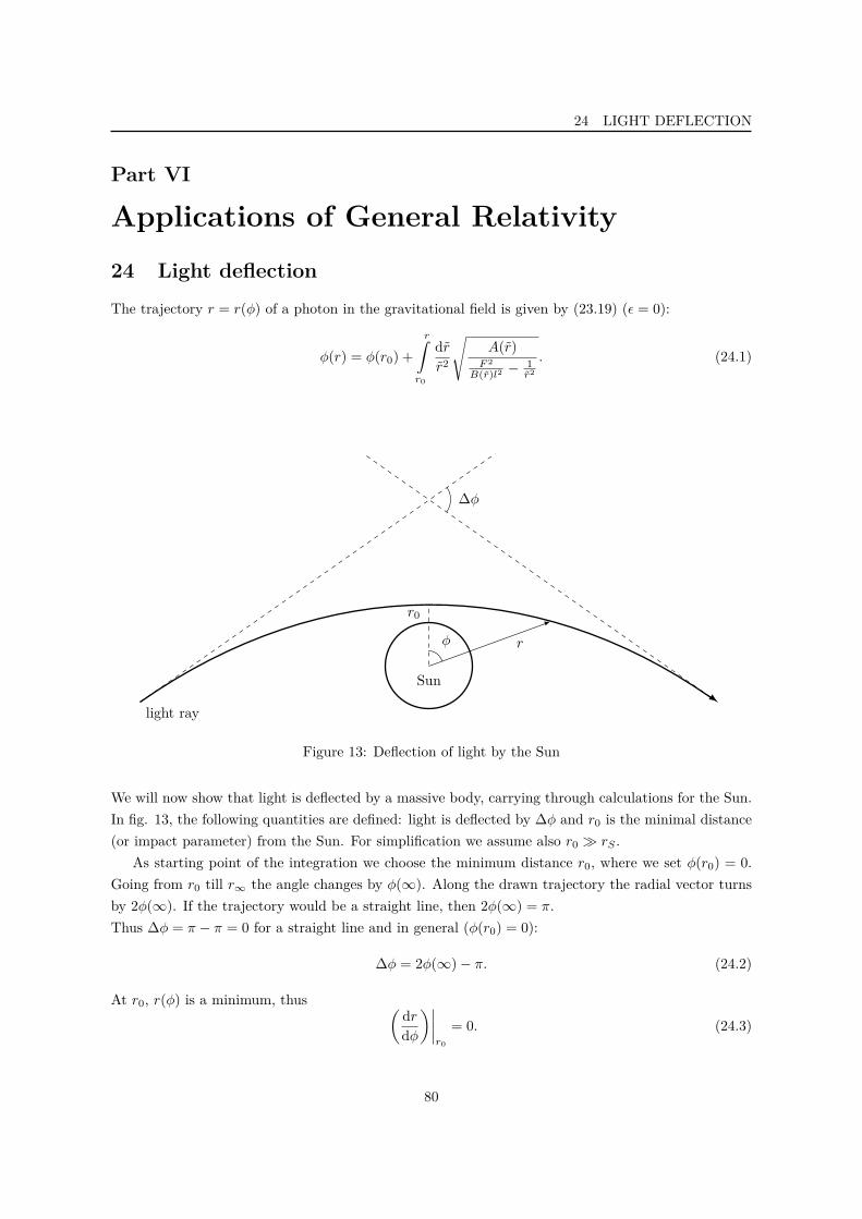
24 LIGHT DEFLECTION
Part VI
Applications of General Relativity24 Light deflection
The trajectory r = r(φ) of a photon in the gravitational field is given by (23.19) (ε = 0):
φ(r) = φ(r0) +r∫
r0
drr2
√A(r)
F 2
B(r)l2 −1r2
. (24.1)
Sun
light ray
r0
rφ
∆φ
Figure 13: Deflection of light by the Sun
We will now show that light is deflected by a massive body, carrying through calculations for the Sun.In fig. 13, the following quantities are defined: light is deflected by ∆φ and r0 is the minimal distance(or impact parameter) from the Sun. For simplification we assume also r0 rS .
As starting point of the integration we choose the minimum distance r0, where we set φ(r0) = 0.Going from r0 till r∞ the angle changes by φ(∞). Along the drawn trajectory the radial vector turnsby 2φ(∞). If the trajectory would be a straight line, then 2φ(∞) = π.Thus ∆φ = π − π = 0 for a straight line and in general (φ(r0) = 0):
∆φ = 2φ(∞)− π. (24.2)
At r0, r(φ) is a minimum, thus (drdφ
)∣∣∣∣r0
= 0. (24.3)
80
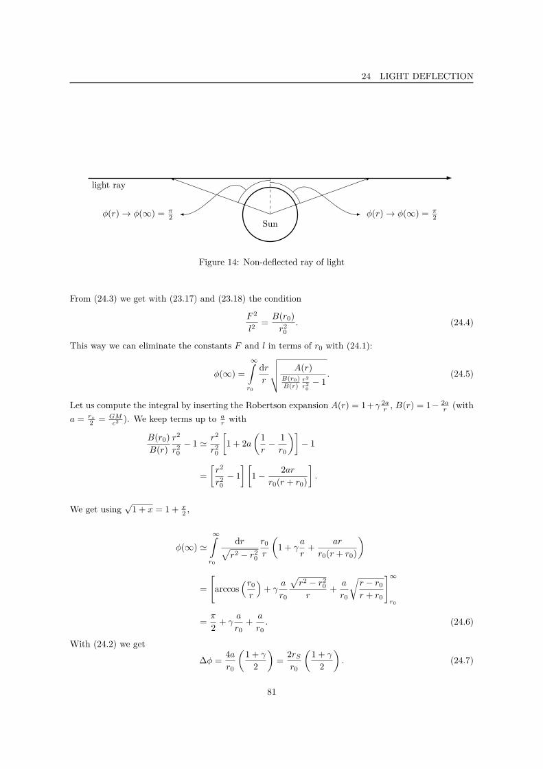
24 LIGHT DEFLECTION
Sun
light ray
φ(r)→ φ(∞) = π2φ(r)→ φ(∞) = π
2
Figure 14: Non-deflected ray of light
From (24.3) we get with (23.17) and (23.18) the condition
F 2
l2= B(r0)
r20
. (24.4)
This way we can eliminate the constants F and l in terms of r0 with (24.1):
φ(∞) =∞∫r0
drr
√√√√ A(r)B(r0)B(r)
r2
r20− 1
. (24.5)
Let us compute the integral by inserting the Robertson expansion A(r) = 1+γ 2ar , B(r) = 1− 2a
r (witha = rs
2 = GMc2 ). We keep terms up to a
r with
B(r0)B(r)
r2
r20− 1 ' r2
r20
[1 + 2a
(1r− 1r0
)]− 1
=[r2
r20− 1] [
1− 2arr0(r + r0)
].
We get using√
1 + x = 1 + x2 ,
φ(∞) '∞∫r0
dr√r2 − r2
0
r0
r
(1 + γ
a
r+ ar
r0(r + r0)
)
=[
arccos(r0
r
)+ γ
a
r0
√r2 − r2
0r
+ a
r0
√r − r0
r + r0
]∞r0
= π
2 + γa
r0+ a
r0. (24.6)
With (24.2) we get
∆φ = 4ar0
(1 + γ
2
)= 2rS
r0
(1 + γ
2
). (24.7)
81
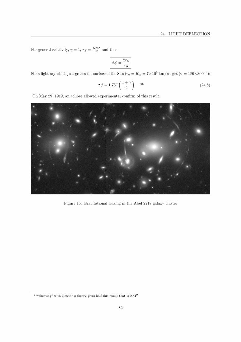
24 LIGHT DEFLECTION
For general relativity, γ = 1, rS = 2GMc2 and thus
∆φ = 2rSr0
For a light ray which just grazes the surface of the Sun (r0 = R = 7×10⁵ km) we get (π = 180×3600′′):
∆φ = 1.75′′(
1 + γ
2
). 26 (24.8)
On May 29, 1919, an eclipse allowed experimental confirm of this result.
Figure 15: Gravitational lensing in the Abel 2218 galaxy cluster
26“cheating” with Newton’s theory gives half this result that is 0.84′′
82
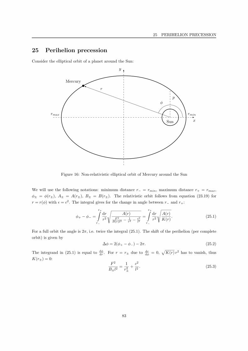
25 PERIHELION PRECESSION
25 Perihelion precession
Consider the elliptical orbit of a planet around the Sun:
x
y
Sun
rminrmax
Mercury
r
φp
Figure 16: Non-relativistic elliptical orbit of Mercury around the Sun
We will use the following notations: minimum distance r− = rmin, maximum distance r+ = rmax,φ± = φ(r±), A± = A(r±), B± = B(r±). The relativistic orbit follows from equation (23.19) forr = r(φ) with ε = c2. The integral gives for the change in angle between r− and r+:
φ+ − φ− =r+∫r−
drr2
√A(r)
F 2
B(r)l2 −1r2 − c2
l2
=r+∫r−
drr2
√A(r)K(r) . (25.1)
For a full orbit the angle is 2π, i.e. twice the integral (25.1). The shift of the perihelion (per completeorbit) is given by
∆φ = 2(φ+ − φ−)− 2π. (25.2)
The integrand in (25.1) is equal to dφdr . For r = r± due to dr
dφ = 0,√K(r) r2 has to vanish, thus
K(r±) = 0:F 2
B±l2= 1r2±
+ c2
l2. (25.3)
83
25 PERIHELION PRECESSION
This way we can express F and l through r±:
F 2
l2=
1r2+− 1
r2−
1B+− 1
B−
=r2− − r2
+
r2+r
2−
(1B+− 1
B−
) , (25.4)
c2
l2= −
B+r2+− B−
r2−
B+ −B−= −
r2+B+− r2
−B−
r2+r
2−
(1B+− 1
B−
) . (25.5)
This leads us to an expression for K(r):
K(r) =r2−
(1
B(r) −1B−
)− r2
+
(1
B(r) −1B+
)r2+r
2−
(1B+− 1
B−
) − 1r2 . (25.6)
For A and B insert the Robertson expansion
A(r) = 1 + γ2ar
+ . . . , (25.7)
B(r) = 1− 2ar
+ 2(β − γ)(ar
)2+ . . . , (25.8)
1B(r) = 1 + 2a
r+ 2(2− β + γ)
(ar
)2+ . . . . 27 (25.9)
With eq. (25.9), K(r) becomes a quadratic form in 1r . Since
dφdr =∞ for r = r±, K+ = K− = 0. This
determines K(r) up to a constant c:
K(r) = c
(1r−− 1r
)(1r− 1r+
). (25.10)
c can be obtained by comparing with (25.6) for r →∞. With (25.9) one gets
c = 1− (2− β + γ)(a
r++ a
r−
). (25.11)
We get thus the following integral:
φ+ − φ− = 1√c
r+∫r−
drr2
(1 + γ
a
r
)︸ ︷︷ ︸
from√A≈ 1+γ ar
[(1r−− 1r
)(1r− 1r+
)]− 12
. (25.12)
We perform the following substitution:
1r
= 12
(1r+
+ 1r−
)+ 1
2
(1r+− 1r−
)sinψ; (25.13)
27 v2
c2≈ a
r; terms g00u0u0 ≈ Bc2 and g11u1u1 ≈ Av2 ≈ Ac2 a
rshow up both and have thus to be expanded to the
same order in ar. Therefore B has to be expanded one order in a
rmore than A.
84
25 PERIHELION PRECESSION
r+ and r− correspond to ψ = π2 and ψ = −π2 , respectively. With
d(
1r
)= − 1
r2 dr = 12
(1r+− 1r−
)cosψ dψ, (25.14)
1r−− 1r
= 12
(1r−− 1r+
)(1 + sinψ), (25.15)
1r− 1r+
= 12
(1r−− 1r+
)(1− sinψ), (25.16)
we get for the integral
φ+ − φ− = 1√c
π2∫
−π2
dψ[1 + γ
a
2
(1r−
+ 1r+
)+ γ
a
2
(1r+− 1r−
)sinψ
]. (25.17)
Now introduce the parameter p of the ellipse (see figure 16):
2p
= 1r+
+ 1r−. (25.18)
Integration of eq. (25.17) leads to
φ+ − φ− = π√c
[1 + γ
a
p
]= π
[1 + (2− β + γ)a
p
] [1 + γ
a
p
]= π
[1 + (2− β + 2γ)a
p
]. (25.19)
Precession per orbit for the perihelion is:
∆φ = 2(φ+ − φ−)− 2π = 6πap
(2− β + 2γ
3
). (25.20)
In general relativity γ = β = 1 and so 2−β+2γ3 = 1. Thus,
∆φ = 6πap
Consider Mercury: p = 55 × 106 km, 2a ≈ 3 km, π = 180 × 3600′′ which give ∆φ = 6πap =
0.104′′ (per full orbit). In 100 years Mercury fulfills 415 orbits around the Sun, this way we get∆φ = 43′′ (per century). For more distant planets (Venus, Earth,. . . ) ∆φ is at most ∼ 5′′ per century.Already in 1882, Newcomb found a perihelion precession of 43′′ per century for Mercury. Full perihelionprecession amounts to 575′′ per century of which 532′′ are due to the influence of other planets (thiswithin Newtonian theory). One finds
2− β + 2γ3 = 1.003± 0.005, (25.21)
in good agreement with general relativity. So far, the parameters of the Robertson expansion areconstrained to |γ − 1| < 3 × 10⁻⁴ and |β − 1| < 3 × 10⁻³. More recently (radar echoes delay fromCassini spacecraft): |γ − 1| = (2.1± 2.3)× 10−5.28
28B. Bertotti et al. Nature 425, 374 (2003)
85

25 PERIHELION PRECESSION
Sun
Mercury
Figure 17: Illustration of the perihelion precession of Mercury (effect strongly exagerated)
25.1 Quadrupole moment of the Sun
A quadrupole moment of the Sun could also influence a perihelion precession of Mercury, that is whyone has to study it. The mass quadrupole moment of the Sun (due to its rotation) is
Q = J2MR2 with J2 = 2
5R‖ −R⊥R
, (25.22)
and
• R‖: orthogonal (to R⊥) radius,
• R⊥: radius orthogonal to the plane containing the planet orbits and parallel to the rotation axisof the Sun.
The induced gravitational potential in the planet’s orbital plane (which is also the equatorial plane ofthe Sun) is
φ(r) = −GMr− GQ
2r3 . (25.23)
The additional term has the same r dependence than the additional relativistic term:
Veff = −GMr
+ l2
2r2 −GMl2
c2r3 . (25.24)
86
26 LIE DERIVATIVE OF THE METRIC AND KILLING VECTORS
With l ∼ pv and v2 ∼ GMp we can compare the two terms (their relative strength)
GQ
GM l2
c2
∼J2R
2
p2 v2
c2
∼J2R
2
pGMc2∼J2R
2
pa.
We see that the full expression for the perihelion precession is given by
∆φ = 6πap
(2− β + 2γ
3 +J2R
2
2ap
). (25.25)
From observations one finds J2 ∼ (1 − 1.7) × 10−7; thus the additional term is J2R2
2ap ≈ 5 × 10⁻⁴,accounting for at most 1/10 of the error given in (25.21) and is thus negligible.
26 Lie derivative of the metric and Killing vectors
Consider the Lie derivative of the metric tensor gµν in the direction of the vector K. According toequation (14.2) we get:
LKgµν = gµν,κKκ + gµκK
κ,ν + gκνK
κ,µ. (26.1)
To rewrite this expression we observe the identities
Kσ = gσµKµ,
Kκ,νgµκ = ∂Kκ
∂xνgµκ = ∂(Kκgµκ)
∂xν−Kκ ∂gµκ
∂xν= ∂Kµ
∂xν−Kκ ∂gµκ
∂xν.
Hence eq. (26.1) can also be written as
LKgσρ = ∂Kσ
∂xρ+ ∂Kρ
∂xσ+Kµ
[∂gρσ∂xµ
− ∂gµσ∂xρ
− ∂gρµ∂xσ
]
= ∂Kσ
∂xρ+ ∂Kρ
∂xσ− 2KµΓµρσ (26.2)
= Kσ;ρ +Kρ;σ.
An infinitesimal coordinate transformation is a symmetry of the metric if LKgµν = 0, thus if
Kσ;ρ +Kρ;σ = 0 (26.3)
Any 4-vector Kσ(x) satisfying this equation will be said to form a Killing vector. 29
Example: Consider a stationary gravitational field, for which there exists coordinates xµ such that thecomponents of gµν do not depend on ct = x0 (for instance Schwarzschild metric). Let Kµ = δµ0 withthe corresponding vector field δµ0∂µ (→ ∂0). Inserting Kµ into (26.1) one gets LKgµν = gµν,0 +0+0 =∂∂x0 gµν = 0 (since gµν does not depend on x0). K is a Killing vector or Killing field or an infinitesimalisometry.
29Named after 19th century mathematician Wilhelm Killing
87

27 MAXIMALLY SYMMETRIC SPACES
Notice that, due to the properties of the Lie derivative, ifK1 andK2 are Killing vectors, LK1gµν = 0,LK2gµν = 0 then [K1,K2] is also a Killing vector since
[LK1 ,LK2 ]gµν = L[K1,K2]gµν = 0. (26.4)
We are used to the fact that symmetries lead to conserved quantities: in classical mechanics the angularmomentum of a particle moving in a rotationally symmetric field is conserved. In the present context,the concept of “symmetries of a gravitational field” is replaced by “symmetries of the metric” and wetherefore expect conserved quantities to be associated with the presence of Killing vectors.
Let Kµ be a Killing vector and xµ(τ) be a geodesic. Then the quantity Kµxµ is constant along the
geodesic. Indeed,
D
dτ(Kµx
µ) = (∇νKµxν)xµ +Kµ (∇ν xµ)︸ ︷︷ ︸
=0 geodesic
xν
= 12 (∇νKµ +∇µKν)︸ ︷︷ ︸
=0 (26.3)
xµxν = 0. (26.5)
Tµν is the covariantly conserved symmetric energy-momentum tensor with ∇µTµν = 0. Then Jµ =TµνKν is a covariantly conserved current:
∇µJµ = (∇µTµν)︸ ︷︷ ︸=0
Kν + Tµν∇µKν = 12T
µν (∇µKν +∇νKµ)︸ ︷︷ ︸=0 (26.3)
= 0,
to which we can associate a conserved charge.
27 Maximally symmetric spaces
Maximally symmetric spaces are spaces that admit the maximal number of Killing vectors (which belowwill turn out to be n(n+1)
2 for an n-dimensional space). In the context of the cosmological principlesuch spaces, which are simultaneously homogeneous (“the same at every point”) and isotropic (“thesame in every direction”), provide a description of space in a cosmological space-time.
From equation (17.2) we had (from definition of Riemann tensor and covariant derivative)
([∇X ,∇Y ]−∇[X,Y ])V λ = RλσµνXµY νV σ, (27.1)
along withX = Xµ∂µ, Y = Y ν∂ν and∇Y ν∂νV λ = Y ν∇∂νV λ = Y ν∇νV λ,∇X∇Y V λ = Xµ∇µ(Y ν∇νV λ) =Xµ(∇µY ν)∇νV λ +XµY ν∇µ∇νV λ etc, we get
[∇µ,∇ν ]V λ = RλσµνVσ. (27.2)
Taking into account the first Bianchi identity, it is possible to find that for a Killing vector Kµ, onehas (no proof here)
∇λ∇µKν(x) = RρλµνKρ(x) (27.3)
88

27 MAXIMALLY SYMMETRIC SPACES
for x = x0. Thus a Killing vector Kµ(x) is completely determined everywhere by the values of Kµ(x0)and ∇µKν(x0) at a single point x0 (think of Taylor expansion). A set of Killing vectors K(i)
µ (x) issaid to be independent if any linear relation of the form∑
i
ciK(i)µ (x) = 0, (27.4)
with constant coefficients ci; implying ci = 0. Since in an n-dimensional space-time there can beat most n linearly independent vectors K(i)
µ (x0) at a point, and at most n(n−1)2 independent anti-
symmetric matrices (∇µKν(x0)), we reach the conclusion that an n-dimensional space-time can haveat most
n+ n(n− 1)2 = n(n+ 1)
2 (27.5)
independent Killing vectors.
• Homogeneous space is meaning that the n-dimensional space(-time) admits n-translational Killingvectors.
• Isotropic space: ∇µKν(x0) is an arbitrary anti-symmetric matrix (→ rotation). We can choosea set of n(n−1)
2 Killing vectors.
• We define a maximally symmetric space to be a space with a metric with a maximal number ofn(n+1)
2 Killing vectors.
The Riemann curvature tensor of a maximally symmetric space becomes simpler. One can show (noproof) that it becomes
Rijkl = k(gikgjl − gilgjk) (27.6)
for some constant k. The Ricci tensor then becomes
Rij(x) = (n− 1)kgij . (27.7)
The Ricci scalar can be obtained to be
R(x) = n(n− 1)k, (27.8)
and the Einstein tensorGik = Rik −
12Rgik = k (n− 1)
(1− n
2
)gik.
The Bianchi identity implies that k is a constant in order for Gik;k to vanish. We shall deal withspace-times in which the metric is spherically symmetric and homogenous on each “plane” of constanttime. In our case n = 4 and the maximally symmetric subspace has 3 dimensions. Consider first themetric on the 3-dimensional subspace
dσ2 = A(r)dr2 + r2 dΩ2︸︷︷︸dθ2+sin2 θdφ2
For the Christoffel symbols, we use the ones for the general form of a static isotropic metric (22.6) withB(r) = 0. Since the Christoffel symbols are invariant under an overall sign change of the metric, also
89

27 MAXIMALLY SYMMETRIC SPACES
the Ricci tensor is and thus one can apply (22.10)-(22.13) with B(r) = 0 for this three-dimensionalspace, without caring for the sign in front of A. Hence we get for equation (27.7)
Rrr = R11 = A′
rA,
Rθθ = R22 = − 1A
+ 1 + rA′
2A2 .
(27.9)
From eq. (27.7), we have Rrr = 2kA, and Rθθ = 2kgθθ = 2kr2. Thus from equating the two firstequation leads us to
2kA = A′
rA⇒ A′ = 2krA2, (27.10)
while we get for the second one
2kr2 = − 1A
+ 1 + rA′
2A2 = − 1A
+ 1 + 2kr2A2
2A2 = − 1A
+ 1 + kr2 ⇒ kr2 = − 1A
+ 1,
which leads toA = 1
1− kr2 , (27.11)
and solves also (27.10). Then the metric on the 3-dimensional subspace (maximally symmetric) is
dσ2 = dr2
1− kr2 + r2dΩ2. (27.12)
It can be shown that k can have the following values: 0, ±1.
k =
+1 sphere, positive curvature
−1 hyperbola, negative curvature
0 plane, zero curvature
The full metric (with time coordinate) has then the form:
ds2 = c2dt2 − a2(t)
dr2
1− kr2 + r2(dθ2 + sin2 θ dφ2)
(27.13)
where a(t) is the cosmic scale factor, which has to be determined by solving the Einstein’s equations viathe matter content of the universe. This metric (first discovered by Friedmann, Lemaître, Roberstonand Walker) is a reasonable ansatz for describing the universe. There is good evidence that the universe(on large scales) is surprisingly homogeneous and isotropic (from redshift surveys of galaxies and cosmicmicrowave background radiation).
90

28 FRIEDMANN EQUATIONS
28 Friedmann equations
We write the metric (27.13) as follows:
ds2 = c2dt2 − a2(t)gij dxi dxj , (28.1)
where tildes denote 3-dimensional quantities calculated with the metric gij . The Christoffel symbolsare given by (notice Γµ00 = 0):
Γijk = Γijk, Γij0 = a
aδij , Γ0
ij = a a gij , (28.2)
where dot denotes derivation with respect to t. The relevant components of the Riemann tensor are:
Ri0j0 = − aaδij , R0
i0j = a a gij , Rkikj = Rij + 2a2 gij (28.3)
We can make use of Rij = 2kgij (maximal symmetry of the 3-dimensional subspace) to compute Rµν .The non-zero components are then
R00 = −3 aa, Rij = (aa+ 2a2 + 2k)gij = −
(a
a+ 2 a
2
a2 + 2 ka2
)gij , (28.4)
where gij = −a2gij . The Ricci scalar becomes R = − 6a2 (aa+ a2 + k) and the non-zero components of
the Einstein tensor are
G00 = 3(a2
a2 + k
a2
), G0i = 0, Gij =
(2 aa
+ a2
a2 + k
a2
)gij . (28.5)
Next we have to specify the matter content. We treat here the universe as non-interacting particles ora perfect fluid. A perfect fluid has energy-momentum tensor (19.8)
Tµν =( pc2
+ ρ)uµuν − gµνp, (28.6)
where p is the pressure, ρ the energy density and uµ the velocity field of the fluid (uµ = (c, 0, 0, 0) ina comoving coordinate system). The trace of the energy-momentum tensor is then
Tµµ = ρc2 − 3p. (28.7)
The equation of state is p = p(ρ) and in particular one assumes
p = wρ, (28.8)
where w is the equation of state parameter.
Examples:
• For non-interacting particles we have p = 0, w = 0. Such matter is referred to as dust. Theenergy-momentum tensor is Tµν = ρ uµuν .
• For radiation the energy-momentum tensor is (like in Maxwell’s theory) traceless and henceradiation has the equation of state
p = 13ρ, (28.9)
thus w = 13 .
91

28 FRIEDMANN EQUATIONS
• As we will see, a cosmological constant Λ corresponds to a “matter” contribution with w = −1.
The conservation law T νµ;µ = 0 implies T 0µ;µ = 0 or ∂µTµ0 + ΓµµνT ν0 + Γ0
µνTµν = 0. For a perfect
fluid: ∂tρ(t)+Γµµ0ρ+Γ000ρ+Γ0
ijTij = 0 (with i, j = 1, 2, 3). Inserting the expressions for the Christoffel
symbols (28.2) we get:ρ = −3(ρ+ p) a
a. (28.10)
For dust (p = 0):ρ
ρ= −3 a
a. (28.11)
Integration gives ρa3 = constant or ρ ∝ a−3. For a radiation dominated universe we get
p = ρ
3 ⇒ρ
ρ= −4 a
a. (28.12)
Integration gives ρa4 = constant or ρ ∝ a−4. More generally for (28.8) one gets:
ρa(t)3(1+w) = constant. (28.13)
The Einstein equations with Λ (equation (20.10)) are
Gµν = 8πGc4
Tµν + Λgµν .
Using (19.8) and that uµ = (c, 0, 0, 0) in a comoving coordinate system, let us write down the 00-component and the ij-component of this equation:
3(a2
a2 + k
a2
)= 8πGρ+ Λ, (28.14)
(2 aa
+ a2
a2 + k
a2
)gij = (−8πGp+ Λ) gij . (28.15)
One has in addition equation (28.10) from the conservation law. Using the first equation to eliminatea2
a2 + ka2 from the second one, one obtains the Friedmann equations:
a2
a2 + k
a2 = 8πG3 ρ+ Λ
3 , (28.16)
−3 aa
= 4πG(ρ+ 3p)− Λ, (28.17)
ρ = −3(ρ+ p) aa. (28.18)
Notice that one could also use the form (20.8) of the Einstein equations to derive the above equations.Introducing the Hubble parameter : H(t) = a(t)
a(t) and the deceleration parameter : q(t) = −a(t)a(t)a2(t) , with
their present day values denoted by H0 = H(t0) and q0 = q(t0), where t0 is the age of the universe;
92
28 FRIEDMANN EQUATIONS
we get instead
H2 = 8πG3 ρ− k
a2 + Λ3
q = 13H2 (4πG(ρ+ 3p)− Λ)
ddt (ρa
3) = −3Hpa3
(28.19)
In the case of Λ = 0, we define a critical density ρcrit = 3H2
8πG and a density parameter Ω = ρρcrit
. Thenρ < ρcrit ⇔ k = −1 open universe
ρ = ρcrit ⇔ k = 0 flat universe
ρ > ρcrit ⇔ k = +1 close universe
Let us now assume that the density is a combination of dust (that we shall simply denote as“matter”) and radiation: ρ = ρm + ρr. Moreover, we assume that ρm ∼ a−3 and ρr ∼ a−4. This isvalid if radiation and matter are decoupled, or if one density is much bigger that the other one (noticethat in today’s universe ρm ρr). Let us introduce the constants Km = 8πG
3 ρma3 and Kr = 8πG
3 ρra4.
Inserting them into equation (28.16) leads to
a2 − Kr
a2 −Km
a− 1
3Λa2 = −k. (28.20)
This equation reads asa2 + V (a) = −k,
whereV (a) = −Kr
a2 −Km
a− 1
3Λa2 (28.21)
plays the role of an effective potential, see figure 18.Consider the solution for a → 0: in that case the terms Kr
a2 and Kma dominate and the behavior
does not depend neither on k nor on Λ.
a2 ≈ Kr
a2 → a(t) ∼√t (28.22)
a2 ≈ Km
a→ a(t) ∼ t 2
3 (28.23)
For a → 0, a goes to ∞. If Kr 6= 0, then for a → 0 a ∼√t. From figure 18 we can discriminate
different types of solutions:
1. For Λ < 0, there is for all k-values a maximal amax. Thus there will be a periodic solution goingbetween a = 0 and amax.
2. Λ = 0 (Einstein-de Sitter universe): for k = 1 there is a bounded solution as in the case 1. Fork = 0 the expansion velocity goes towards 0, instead for k = −1 it goes towards a constant value.
3. For Λ > 0 there are several cases:
93

28 FRIEDMANN EQUATIONS
a) Λ = Λcrit and k = 1. The value of Λcrit is obtained for the horizontal line −k (figure 18)just going through the maximum of the potential. Assuming Kr ≈ 0 (as in today’s universe)we get with a = 0, V = −1 → dV
da = 0:
Λ = Λcrit = 49K2
m
and a = astat = 3Km
2 . (28.24)
This corresponds to the static Einstein solution. Einstein introduced a cosmological constantin order to get such a static solution, which is however unstable. Small perturbations leadeither to a contraction or to an exponential growth.
b) Λ < Λcrit and k = 1. The horizontal line −k intercepts the curve V (a) in two points a1 anda2. We obtain either a periodic solution between 0 and a1 or an unbounded solution witha > a2.
c) Λ = Λcrit(1 + ε) and k = 1. For 0 < ε 1 the horizontal line −k lies just above themaximum value of V (a). Thus the expansion velocity a will be very low in this region(Lemaître universe).
d) Λ > Λcrit and k = 1. The line −k does not intercept the V (a) curve. Around the maximumof V (a) the expansion is lowered.
e) Λ > 0 and k = −1, 0 : as in the previous case, but there may be less deceleration in theregion of the maximum of V (a).
a
V
Λ < 0
Λ > 0
Λ = 0
−k
Figure 18: Sketch of the “effective potential” V (a) for different values of Λ.
For Λ > 0, all solutions are unbounded. In the limit a→∞, V (a) is dominated by the Λ-term:
a2 ≈ Λ3 a
2,
94
28 FRIEDMANN EQUATIONS
thus
a(t) ∼ exp(√
Λ3 t). (28.25)
The expansion is exponentially accelerated.According to the currently most accepted model (so-called ΛCDM-model), the main contributions
to the density are
• ordinary matter (baryons) Ωbaryons ∼ 0.05
• dark matter ΩDM ∼ 0.27
• cosmological constant ΩΛ = ρΛρcrit∼ 0.68 with ρΛ = Λ
8πG (also called dark energy).
Moreover, the universe seems to be almost flat: k ≈ 0. These cosmological parameters would thuscorrespond to the case 3e) of the previous discussion.
Finally, H−10 is related to the age of the universe. H0 ∼ 67.80± 0.77 km
sec/Mpc gives an age of ∼ 13.8billion years.30
30Planck 2013 results. XVI. Cosmological parameters - http://arxiv.org/abs/1303.5076
95