Generating Polyphonic Music Using Tied ParallelNetworks

Daniel D. Johnson

Harvey Mudd CollegeClaremont, CA 91711 USAddjohnson@hmc.edu

Abstract. We describe a neural network architecture which enables predictionand composition of polyphonic music in a manner that preserves translation-invariance of the dataset. Specifically, we demonstrate training a probabilisticmodel of polyphonic music using a set of parallel, tied-weight recurrent networks,inspired by the structure of convolutional neural networks. This model is designedto be invariant to transpositions, but otherwise is intentionally given minimal in-formation about the musical domain, and tasked with discovering patterns presentin the source dataset. We present two versions of the model, denoted TP-LSTM-NADE and BALSTM, and also give methods for training the network and forgenerating novel music. This approach attains high performance at a musical pre-diction task and successfully creates note sequences which possess measure-levelmusical structure.

1 Introduction

There have been many attempts to generate music algorithmically, including Markovmodels, generative grammars, genetic algorithms, and neural networks; for a surveyof these approaches, see Nierhaus [17] and Fernandez and Vico [5]. Neural networkmodels are particularly flexible because they can be trained based on the complex pat-terns in an existing musical dataset, and a wide variety of neural-network-based musiccomposition models have been proposed [1, 7, 14, 16, 22].

One particularly interesting approach to music composition is training a probabilis-tic model of polyphonic music. Such an approach attempts to model music as a proba-bility distribution, where individual sequences are assigned probabilities based on howlikely they are to occur in a musical piece. Importantly, instead of specifying particularcomposition rules, we can train such a model based on a large corpus of music, and al-low it to discover patterns from that dataset, similarly to someone learning to composemusic by studying existing pieces. Once trained, the model can be used to generate newmusic based on the training dataset by sampling from the resulting probability distribu-tion.

Training this type of model is complicated by the fact that polyphonic music hascomplex patterns along multiple axes: there are both sequential patterns between timestepsand harmonic intervals between simultaneous notes. Furthermore, almost all musicalstructures exhibit transposition invariance. When music is written in a particular key,the notes are interpreted not based on their absolute position but instead relative to that

particular key, and chords are also often classified based on their position in the key (e.g.using Roman numeral notation). Transposition, in which all notes and chords are shiftedinto a different key, changes the absolute position of the notes but does not change anyof these musical relationships. As such, it is important for a musical model to be ableto generalize to different transpositions.

Recurrent neural networks (RNN), especially long short-term memory networks(LSTM) [8], have been shown to be extremely effective at modeling single-dimensionaltemporal patterns. It is thus reasonable to consider using them to model polyphonic mu-sic. One simple approach is to treat all of the notes played at any given timestep as asingle input vector, and train an LSTM network to output a vector of probabilities ofplaying each note in the next timestep [4]. This essentially models each note as an inde-pendent event. While this may be appropriate for simple inputs, real-world polyphonicmusic contains complex harmonic relationships that would be better described using ajoint probability distribution. To this end, a more effective approach combines RNNsand restricted Boltzmann machines to model the joint probability distribution of notesat each timestep [3].

Although both of the above approaches enable a network to generate music in asequential manner, neither are transposition-invariant. In both, each note is representedas a separate element in a vector, and thus there is no way for the network to general-ize intervals and chords: any relationship between, say, a G and a B, must be learnedindependently from the relationship between a G[ and a B[. To capture the structureof chords and intervals in a transposition-invariant way, a neural network architecturewould ideally consider relative positions of notes, as opposed to absolute positions.

Convolutional neural networks, another type of network architecture, have provento be very adept at feature detection in image recognition; see Krizhevsky et al. [12] forone example. Importantly, image features are also multidimensional patterns which areinvariant over shifts along multiple axes, the x and y axes of the image. Convolutionalnetworks enable invariant feature detection by training the weights of a convolutionkernel, and then convolving the image with the kernel.

Combining recurrent neural networks with convolutional structure has shown promisein other multidimensional tasks. For instance, Kalchbrenner et al. [10] describe an ar-chitecture involving LSTMs with simultaneous recurrent connections along multipledimensions, some of which may have tied weights. Additionally, Kaiser and Sutskever[9] present a multi-layer architecture using a series of “convolutional gated recurrentunits”. Both of these architectures have had success in tasks such as digit-by-digit mul-tiplication and language modeling.

In the current work, we describe two variants of a recurrent network architecture in-spired by convolution that attain transposition-invariance and produce joint probabilitydistributions over a musical sequence. These variations are referred to as Tied Paral-lel LSTM-NADE (TP-LSTM-NADE) and Biaxial LSTM (BALSTM). We demonstratethat these models enable efficient encoding of both temporal and pitch patterns by usingthem to predict and generate musical compositions.

1.1 LSTM

Long Short-Term Memory (LSTM) is a sophisticated architecture that has been shownto be able to learn long-term temporal sequences [8]. LSTM is designed to obtain con-stant error flow over long time periods by using Constant Error Carousels (CECs),which have fixed-weight recurrent connections to prevent exploding or vanishing gra-dients. These CECs are connected to a set of nonlinear units that allow them to interfacewith the rest of the network: an input gate determines how to change the memory cells,an output gate determines how strongly the memory cells are expressed, and a forgetgate allows the memory cells to forget irrelevant values. The formulas for the activationof a single LSTM block with inputs xt and hidden recurrent activations ht at timestept are given below:

zt = tanh(Wxzxt +Whzht−1 + bz) block inputit = σ(Wxixt +Whiht−1 + bi) input gateft = σ(Wxfxt +Whfht−1 + bf ) forget gatect = it � zt + ft � ct−1 cell stateot = σ(Wxoxt +Whoht−1 + bo) output gateht = ot � tanh(ct) output

where W denotes a weight matrix, b denotes a bias vector, � denotes elementwise vec-tor multiplication, and σ and tanh represent the logistic sigmoid and hyperbolic tangentelementwise activation functions, respectively. We are omitting so-called “peephole”connections, which use the contents of the memory cells as inputs to the gates. Theseconnections have been shown not to have a significant impact on the network perfor-mance [6]. Like traditional RNN, LSTM networks can be trained by backpropagationthrough time (BPTT), or by truncated BPTT. Figure 1 gives a schematic of an LSTMblock.

tanh

σ σ σ

tanh

z

i

c

fo

h

Fig. 1. Schematic of a LSTM block. Dashed lines represent a one-timestep delay. Solid arrowinputs represent xt, and dashed arrow inputs represent ht−1, each of which are scaled by learnedweights (not shown). ⊕ indicates a sum, and � indicates elementwise multiplication.

1.2 RNN-NADE

The RNN-RBM architecture, as well as the closely related RNN-NADE architecture,are attempts to model the joint distribution of a multidimensional sequence [3]. Specif-ically, the RNN-RBM combines recurrent neural networks (RNNs), which can capturetemporal interactions, and restricted Boltzmann machines (RBMs), which model con-ditional distributions.

RBMs have the disadvantage of having a gradient that is untractable to compute:the gradients of the loss with respect to the model parameters must be estimated byusing a method such as contrastive divergence or Gibbs sampling. To obtain a tractablegradient, the RNN-NADE architecture replaces the RBM with a neural autoregressivedistribution estimator (NADE) [13], which calculates the joint probability of a vectorof binary variables v = [v1, v2, · · · , vn] (here used to represent the set of notes that arebeing played simultaneously) using a series of conditional distributions:

p(v) =

|v|∏i=1

p(vi|v<i)

with each conditional distribution given by

hi = σ(bh +W:,<iv<i)

p(vi = 1|v<i) = σ(bvi + Vi,:hi)

p(vi = 0|v<i) = 1− p(vi = 1|v<i)

where bv and bh are bias vectors and W and V are weight matrices. Note that v<idenotes the vector composed of the first i− 1 elements of v, W:,<i denotes the matrixcomposed of all rows and the first i− 1 columns of W , and Vi,: denotes the ith row ofV . Under this distribution, the loss has a tractable gradient, so no gradient estimation isnecessary.

In the RNN-NADE, the bias parameters bv and bh at each timestep are calculatedusing the hidden activations h of an RNN, which takes as input the output v of thenetwork at each timestep:

h(t) = σ(Wvhv(t) +Whhh

(t−1) + bh)

b(t)v = bv +Whbv

h(t)

b(t)h = bh +Whbh

h(t)

The RNN parametersWvh,Whh, bv ,Whbv, bh,Whbh

, as well as the NADE parametersW and V are all trained using stochastic gradient descent.

2 Translation Invariance and Tied Parallel Networks

One disadvantage of distribution estimators such as RBM and NADE is that they can-not easily capture relative relationships between inputs. Although they can readily learn

relationships between any set of particular notes, they are not structured to allow gen-eralization to a transposition of those notes into a different key. This is problematic forthe task of music prediction and generation because the consonance or dissonance of aset of notes remains the same regardless of their absolute position.

As one example of this, if we represent notes as a one-dimensional binary vector,where a 1 represents a note being played, a 0 represents a note not being played, andeach adjacent number represents a semitone (half-step) increase, a major chord can berepresented as

. . . 001000100100 . . .

This pattern is still a major chord no matter where it appears in the input sequence, so

1000100100000,

0010001001000,

0000010001001,

all represent major chords, a property known as translation invariance. However, if theinput is simply presented to a distribution estimator such as NADE, each transposedrepresentation would have to be learned separately.

Convolutional neural networks address the invariance problem for images by con-volving or cross-correlating the input with a set of learned kernels. Each kernel learns torecognize a particular local type of feature. The cross-correlation of two one-dimensionalsequences u and v is given by

(u ? v)n =

∞∑m=−∞

umvm+n.

Crucially, if one of the inputs (say u) is shifted by some offset δ, the output (u ? v)nis also shifted by δ, but otherwise does not change. This makes the operation ideal fordetecting local features for which the relevant relationships are relative, not absolute.

For our music generation task, we can obtain transposition invariance by designingour model to behave like a cross-correlation: if we have a vector of notes v(t) at timestept and a candidate vector of notes v(t+1) for the next timestep, and we construct shiftedvectors w(t) and w(t+1) such that w(t)

i = v(t)i+δ and w

(t+1)i = v

(t+1)i+δ , then we want the

output of our model to satisfy

p(w(t+1)|w(t)) = p(v(t+1)|v(t)).

2.1 Tied Parallel LSTM-NADE

In order to achieve the above form of transposition invariance, but also handle complextemporal sequences and jointly-distributed output, we propose dividing the music pre-diction task into a set of tied parallel networks. Each network instance will be respon-sible for a single note, and will have tied weights with every other network instance. Inthis way, we ensure translation invariance: since each instance uses the same procedureto calculate its output, if we shift the inputs up by some amount δ, the output will also

Fig. 2. Illustration of the windowing and binning operations. The thick-outlined box representsthe current note. On the left, a local window around the note is extracted, and on the right, notesfrom each octave are binned together according to their pitchclass. For clarity, an octave is repre-sented here by four notes; in the actual implementation octaves are of size 12.

be shifted by δ. Our task is thus to divide the RNN-NADE architecture into multiplenetworks in this fashion, while still maintaining the ability to model notes conditionallyon past output.

In the original RNN-NADE architecture, the RNN received the entire note vectoras input. However, since each note now has a network instance that operates relativeto that note, it is no longer feasible to give the entire note vector v(t) as input to eachnetwork instance. Instead, we will feed the instance two input vectors, a local windoww(n,t) and a set of bins z(n,t). The local window contains a slice of the note vector v(t)

such that w(n,t)i = v

(t)n−13+i where 1 ≤ i ≤ 25 (giving the window a span of one octave

above and below the note). If the window extends past the bounds of v, those values areinstead set to 0, as no notes are played above or below the bounds of v. The content ofeach bin zi is the number of notes that are played at the offset i from the current noteacross all octaves:

z(n,t)i =

∞∑m=−∞

v(t)i+n+12m

where, again, v is assumed to be 0 above and below its bounds. This is equivalent to col-lecting all notes in each pitchclass, measured relative to the current note. For instance,if the current note has pitchclass D, then bin z2 will contain the number of played noteswith pitchclass E across all octaves. The windowing and binning operations are illus-trated in Figure 2.

Finally, although music is mostly translation-invariant for small shifts, there is adifference between high and low notes in practice, so we also give as input to each

network instance the MIDI pitch number it is associated with. These inputs are con-catenated and then fed to a set of LSTM layers, which are implemented as describedabove. Note that we use LSTM blocks instead of regular RNNs to encourage learninglong-term dependencies.

As in the RNN-NADE model, the output of this parallel network instance should bean expression for p(vn|v<n). We can adapt the equations of NADE to enable them towork with the parallel network as follows:

hn = σ(b(n,t)h +Wxn)

p(t)(vn = 1|v<n) = σ(b(n,t)v + V hn)

p(t)(vn = 0|v<n) = 1− p(t)(vn = 1|v<n)

where xn is formed by taking a 2-octave window of the most recently chosen notes,concatenated with a set of bins. This is performed in the same manner as for the inputto the LSTM layers, but instead of spanning the entirety of the notes from the previoustimestep, it only uses the notes in v<n. The parameters b(n,t)

h and b(n,t)v are computedfrom the final hidden activations y(n,t) of the LSTM layers as

b(n,t)v = bv +Wybvy(n,t)

b(n,t)h = bh +Wybhy

(n,t)

One key difference is that bv is now a scalar, not a vector, since each instance of thenetwork only produces a single output probability, not a vector of them. The full outputvector is formed by concatenating the scalar outputs for each network instance. The leftside of Figure 3 is a diagram of a single instance of this parallel network architecture.This version of the architecture will henceforth be referred to as Tied-Parallel LSTM-NADE (TP-LSTM-NADE).

2.2 Bi-axial LSTMs

A downside to the architecture described in Section 2.1 is that, in order to apply themodified NADE, we must use windowed and binned summaries of note output. Thiscaptures some of the most important relationships between notes, but also prevents thenetwork from learning any precise dependencies that extend past the size of the window.As an alternative, we can replace the NADE portion of the network with LSTMs thathave recurrent connections along the note axis. This combination of LSTMs along twodifferent axes (first along the time axis, and then along the note axis) will be referred toas a “bi-axial” configuration, to differentiate it from bidirectional configurations, whichrun recurrent networks both forward and backward along the same axis.

In each “note-step”, these note-axis LSTM layers receive as input a concatenationof two sources: the activations of the final time-axis LSTM layer for this note, andalso the final output of the network for the previous note. The final activations of thenote-axis LSTM will be transformed into a probability p(n,t)(vn = 1|v<n) using soft-max activation. Note that, just as each note has a corresponding tied-weight time-axisLSTM network responsible for modeling temporal relationships for that single note,

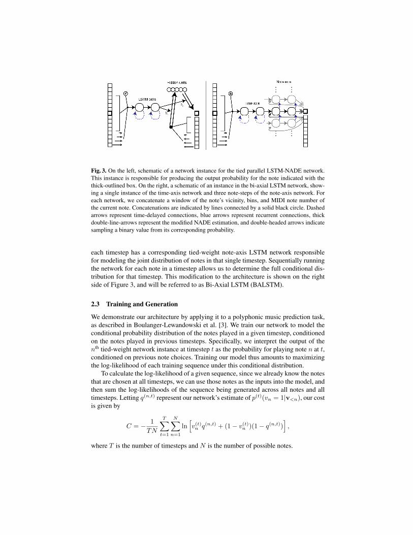
Fig. 3. On the left, schematic of a network instance for the tied parallel LSTM-NADE network.This instance is responsible for producing the output probability for the note indicated with thethick-outlined box. On the right, a schematic of an instance in the bi-axial LSTM network, show-ing a single instance of the time-axis network and three note-steps of the note-axis network. Foreach network, we concatenate a window of the note’s vicinity, bins, and MIDI note number ofthe current note. Concatenations are indicated by lines connected by a solid black circle. Dashedarrows represent time-delayed connections, blue arrows represent recurrent connections, thickdouble-line-arrows represent the modified NADE estimation, and double-headed arrows indicatesampling a binary value from its corresponding probability.

each timestep has a corresponding tied-weight note-axis LSTM network responsiblefor modeling the joint distribution of notes in that single timestep. Sequentially runningthe network for each note in a timestep allows us to determine the full conditional dis-tribution for that timestep. This modification to the architecture is shown on the rightside of Figure 3, and will be referred to as Bi-Axial LSTM (BALSTM).

2.3 Training and Generation

We demonstrate our architecture by applying it to a polyphonic music prediction task,as described in Boulanger-Lewandowski et al. [3]. We train our network to model theconditional probability distribution of the notes played in a given timestep, conditionedon the notes played in previous timesteps. Specifically, we interpret the output of thenth tied-weight network instance at timestep t as the probability for playing note n at t,conditioned on previous note choices. Training our model thus amounts to maximizingthe log-likelihood of each training sequence under this conditional distribution.

To calculate the log-likelihood of a given sequence, since we already know the notesthat are chosen at all timesteps, we can use those notes as the inputs into the model, andthen sum the log-likelihoods of the sequence being generated across all notes and alltimesteps. Letting q(n,t) represent our network’s estimate of p(t)(vn = 1|v<n), our costis given by

C = − 1

TN

T∑t=1

N∑n=1

ln[v(t)n q(n,t) + (1− v(t)n )(1− q(n,t))

],

where T is the number of timesteps and N is the number of possible notes.

Importantly, in each of the variants of our architecture described above, interactionbetween layers flows in a single direction; i.e. the LSTM time-axis layers depend onlyon the chosen notes, not on the specific output of the note-axis layers. During training,we already know all of the notes at all timesteps, so we can accelerate our training pro-cess by processing each layer independently: first preprocessing the input, then runningit through the LSTM time-axis layers in parallel across all notes, and finally either usingthe modified NADE or the LSTM note-axis layers to compute probabilities in parallelacross all timesteps. This massively parallel training process is ideal for training on aGPU or on a multi-core system.

Once trained, we can sample from this trained distribution to “compose” novel se-quences. In this case, we do not know the entire sequence in advance. Instead, we mustrun the full network one timestep at a time. At each timestep, we process the input forthat timestep, advance the LSTM time-axis layers by one timestep, and then generatethe next timestep’s notes. To do this, we sample from the conditional distribution asit is being generated: for each note, we choose v(t)n from a Bernoulli distribution withprobability q(n,t). Then, this choice is used to construct the input for the computationof q(n+1,t). Once all of the notes have been processed, we can advance to the nexttimestep.

The bottleneck of sampling from the distribution before processing the next timestepmakes generation slower on GPUs or multi-core systems, since we can no longer paral-lelize the activation of note-axis computation. However, this can be mitigated somewhatby generating multiple samples simultaneously.

3 Experiments

3.1 Quantitative Analysis

We evaluated two variants of the tied-weight parallel model, along with a non-parallelmodel for comparison:

– LSTM-NADE: Non-parallel model consisting of an LSTM block connected to NADEas in the RNN-NADE architecture. We used two LSTM layers with 300 nodes each,and 150 hidden units in the NADE layer.

– TP-LSTM-NADE: Tied-parallel LSTM-NADE model described in Section 2.1. Weused two LSTM layers with 200 nodes each, and 100 hidden units in the modifiedNADE layer.

– BALSTM: Bi-axial LSTM with windowed+binned input, described in Section 2.2.We used two LSTM layers in the time-axis direction with 200 nodes each, and twoLSTM layers in the note-axis direction with 100 nodes each.We tested the ability of each model to predict/generate note sequences based on four

datasets: JSB Chorales, a corpus of 382 four-part chorales by J.S. Bach; MuseData1, anelectronic classical music library, from CCARH at Stanford; Nottingham2, a collectionof 1200 folk tunes in ABC notation, consisting of a simple melody on top of chords;and Piano-Midi.de, a classical piano MIDI database. Each dataset was transposed into C

1 www.musedata.org2 ifdo.ca/%7Eseymour/nottingham/nottingham.html

Table 1. Log-likelihood performance for the non-transposed prediction task. Data above the lineis taken from Boulanger-Lewandowski et al. [3] and Vohra et al. [25]. Below the line, the twovalues represent the best and median performance across 5 trials.

Model JSB Chorales MuseData Nottingham Piano-Midi.de

Random -61.00 -61.00 -61.00 -61.00RBM -7.43 -9.56 -5.25 -10.17NADE -7.19 -10.06 -5.48 -10.28RNN-RBM -7.27 -9.31 -4.72 -9.89RNN (HF) -8.58 -7.19 -3.89 -7.66RNN-RBM (HF) -6.27 -6.01 -2.39 -7.09RNN-DBN -5.68 -6.28 -2.54 -7.15RNN-NADE (HF) -5.56 -5.60 -2.31 -7.05DBN-LSTM -3.47 -3.91 -1.32 -4.63

LSTM-NADE -6.00, -6.10 -5.02, -5.03 -2.02, -2.06 -7.36, -7.39TP-LSTM-NADE -5.88, -5.92 -4.32, -4.34 -1.61, -1.64 -5.44, -5.49BALSTM -5.05, -5.86 -3.90, -4.41 -1.55, -1.62 -4.90, -5.00

Table 2. Log-likelihood performance for the transposed prediction task. The two values representthe best and median performance across 5 trials.

Model JSB Chorales MuseData Nottingham Piano-Midi.de

LSTM-NADE -9.04, -9.16 -5.72, -5.76 -3.65, -3.70 -8.11, -8.13TP-LSTM-NADE -5.89, -5.92 -4.32, -4.33 -1.61, -1.64 -5.44, -5.49BALSTM -5.08, -5.87 -3.91, -4.45 -1.56, -1.71 -4.92, -5.01

major or C minor and segmented into training, validation, and test sets as in Boulanger-Lewandowski et al. [3]. Input was provided to our network in a piano-roll format, witha vector of length 88 representing the note range from A0 to C8.

Dropout of 0.5 was applied to each LSTM layer, as in Moon et al. [15], and trainedusing RMSprop [21] with a learning rate of 0.001 and Nesterov momentum [19] of 0.9.We then evaluated our models using three criteria. Quantitatively, we evaluated the log-likelihood of the test set, which characterizes the accuracy of the model’s predictions.Qualitatively, we generated sample sequences as described in section 2.3. Finally, tostudy the translation-invariance of the models, we evaluated the log-likelihood of a ver-sion of the test set transposed into D major or D minor. Since such a transposition shouldnot affect the musicality of the pieces in the dataset, we would expect a good model ofpolyphonic music to predict the original and transposed pieces with similar levels ofaccuracy. However, a model that was dependent on its input being in a particular keywould not be able to generalize well to transpositions of the input.

Table 1 shows the performance on the non-transposed task. Data below the linecorresponds to the architectures described here, where the two values represent thebest and median performance of each architecture, respectively, across 5 trials. Dataabove the line is taken from Vohra et al. [25] (for RNN-DBN and DBN-LSTM) andBoulanger-Lewandowski et al. [3] (for all other models). In particular, “Random” shows

the performance of choosing to play each note with 50% probability, and the otherarchitectures are variations of the original RNN-RBM architecture, which we do notdescribe thoroughly here.

Our tied-parallel architectures (BALSTM and TP-LSTM-NADE) perform notice-ably better on the test set prediction task than did the original RNN-NADE model andmany architectures closely related to it. Of the variations we tested, the BALSTM net-work appeared to perform the best. The TP-LSTM-NADE network, however, appears tobe more stable, and converges reliably to a relatively consistent cost. Both tied-parallelnetwork architectures perform comparably to or better than the non-parallel LSTM-NADE architecture.

The DBN-LSTM model, introduced by Vohra et al. [25], has superior performancewhen compared to our tied-parallel architectures. This is likely due to the deep beliefnetwork used in the DBN-LSTM, which allows the DBN-LSTM to capture a richer jointdistribution at each timestep. A direct comparison between the DBN-LSTM model andthe BALSTM or TP-LSTM-NADE models may be somewhat uninformative, since themodels differ both in the presence or absence of parallel tied-weight structure as well asin the complexity of the joint distribution model at each timestep. However, the successof both models relative to the original RNN-RBM and RNN-NADE models suggeststhat a model that combined parallel structure with a rich joint distribution might attaineven better results.

Note that when comparing the results from the LSTM-NADE architecture and theTP-LSTM-NADE/BALSTM architectures, the greatest improvements are on the Muse-Data and Piano-Midi.de datasets. This is likely due to the fact that those datasets containmany more complex musical structures in different keys, which are an ideal case for atranslation-invariant architecture. On the other hand, the performance on the datasetswith less variation in key is somewhat less impressive.

In addition, as shown in Table 2, the TP-LSTM-NADE/BALSTM architecturesdemonstrate the desired translation invariance: both parallel models perform compa-rably on the original and transposed datasets, whereas the non-parallel LSTM-NADEarchitecture performs worse at modeling the transposed dataset. This indicates that theparallel models are able to learn musical patterns that generalize to music in multiplekeys, and are not sensitive to transpositions of the input, whereas the non-parallel modelcan only learn patterns with respect to a fixed key. Although we were unable to eval-uate other existing architectures on the transposed dataset, it is reasonable to suspectthat they would also show reduced performance on the transposed dataset for reasonsdescribed in section 2.

3.2 Qualitative Analysis

In addition to the above experiments, we trained the BALSTM model on a larger col-lection of MIDI pieces with the goal of producing novel musical compositions. To thisend, we made a few modifications to the BALSTM model.

Firstly, we used a larger subset of the Piano-Midi.de dataset for training, includingadditional pieces not used with prior models and pieces originally used as part of thevalidation set. To allow the network to learn rhythmic patterns, we restricted the datasetto pieces with the 4/4 time signature. We did not transpose the pieces into a common

key, as the model is naturally translation invariant and does not benefit from this mod-ification. Using the larger dataset maximizes the variety of pieces used during trainingand was intended to allow the network to learn as much about the musical structures aspossible.

Secondly, the input to the network was augmented with a “temporal position” vec-tor, giving the position of the timestep relative to a 4/4 measure in binary format. Thisgives the network the ability to learn specific temporal patterns relative to a measure.

Thirdly, we added a dimension to the note vector v to distinguish rearticulating anote from sustaining it. Instead of having a single 1 represent a note being played and a0 represent that note not being played, we appended an additional 1 or 0 depending onwhether that note is being articulated at that timestep. Thus the first timestep for playinga note is represented as 11, whereas sustaining a previous note is represented as 10,and resting is represented as 00. This adjustment enables the network to play the samenote multiple times in succession. On the input side, the second bit is preprocessed inparallel with the first bit, and is passed into the time-axis LSTM layers as an additionalinput. On the output side, the note-axis LSTM layers output two probabilities insteadof just one: both the probability of playing a note, and the probability of rearticulatingthe note if the network chooses to play it. When computing the log-likelihood of thesequence, we penalize the network for articulating a played note incorrectly, but ignorethe articulation output for notes that should not be played. Similarly, when generating apiece, we only allow the network to articulate notes that have been chosen to be played.

Qualitatively, the samples generated by this version of the model appear to possesscomplexity and intricacy. Samples from the extended BALSTM model demonstraterhythmic consistency, chords, melody, and counterpoint not found in the samples fromthe RNN-RBM and RNN-NADE models (as provided by Boulanger-Lewandowski etal. [3]). The samples also seem to possess consistency across multiple measures, andalthough they frequently change styles, they exhibit smooth transitions from one styleto another.

A portion of a generated music sample is shown in Figure 4. Samples of the gener-ated music for each architecture can be found on the author’s website. 3

4 Future Work

One application of the music prediction task is improving automatic transcription bygiving an estimate for the likelihood of various configurations of notes [18]. As themusic to be transcribed may be in any key, applying a tied parallel architecture to thistask might improve the results.

A noticeable drawback of our model is that long-term phrase structure is absentfrom the output. This is likely because the model is trained to predict and composemusic one timestep at a time. As a consequence, the model is encouraged to pay moreattention to recent notes, which are often the best predictors of the next timestep, in-stead of on planning long-term structures. Modeling this structure will likely requireincorporating a long-term planning component into the architecture. One approach to

3 https://www.cs.hmc.edu/%7Eddjohnson/tied-parallel/

combining long-term planning with recurrent networks is the Strategic Attentive Writer(STRAW) model, described by Vezhnevets et al. [24], which extends a recurrent net-work with an action plan, which it can modify incrementally over time. Combining suchan approach with a RNN-based music model might allow the model to generate pieceswith long-term structure.

We also noticed that the network occasionally appears to become “confused” afterplaying a discordant note. This is likely because the dataset represents only a small por-tion of the overall note-sequence state space, so it is difficult to recover from mistakesdue to the lack of relevant training data. Bengio et al. [2] proposed a scheduled samplingmethod to alleviate this problem, and a similar modification could be made here.

Another potential avenue for further research is modeling a latent musical stylespace using variational inference [11], which would allow the network to model distinctstyles without alternating between them, and might allow the network to generate musicthat follows a predetermined musical form.

5 Conclusions

In this paper, we discussed the property of translation invariance of music, and proposeda set of modifications to the RNN-NADE architecture to allow it to capture relativedependencies of notes. The modified architectures, which we call Tied-Parallel LSTM-NADE and Bi-Axial LSTM, divide the music generation and prediction task such thateach network instance is responsible for a single note and receives input relative to thatnote, a structure inspired by convolutional networks.

Experimental results demonstrate that this modification yields a higher accuracy ona prediction task when compared to similar non-parallel models, and approaches stateof the art performance. As desired, our models also possess translation invariance, asdemonstrated by performance on a transposed prediction task. Qualitatively, the outputof our model has measure-level structure, and in some cases successfully reproducescomplex rhythms, melodies, and counterpoint.

Although the network successfully models measure-level structure, it unfortunatelydoes not appear to produce consistent phrases or maintain style over a long periodof time. Future work will explore modifications to the architecture that could enablea neural network model to incorporate specific styles and long-term planning into itsoutput.

6 Acknowledgments

We would like to thank Dr. Robert Keller for helpful discussions and advice. We wouldalso like to thank the developers of the Theano framework [20], which we used torun our experiments, as well as Harvey Mudd College for providing computing re-sources. This work used the Extreme Science and Engineering Discovery Environment(XSEDE) [23], which is supported by National Science Foundation grant number ACI-1053575.

References

[1] Bellgard, M.I., Tsang, C.P.: Harmonizing music the boltzmann way. Connection Science6(2-3), 281–297 (1994)

[2] Bengio, S., Vinyals, O., Jaitly, N., Shazeer, N.: Scheduled sampling for sequence predictionwith recurrent neural networks. In: Advances in Neural Information Processing Systems.pp. 1171–1179 (2015)

[3] Boulanger-Lewandowski, N., Bengio, Y., Vincent, P.: Modeling temporal dependencies inhigh-dimensional sequences: Application to polyphonic music generation and transcrip-tion. In: Proceedings of the 29th International Conference on Machine Learning (ICML-12). pp. 1159–1166 (2012)

[4] Eck, D., Schmidhuber, J.: A first look at music composition using LSTM recurrent neuralnetworks. Istituto Dalle Molle Di Studi Sull Intelligenza Artificiale (2002)

[5] Fernandez, J.D., Vico, F.: Ai methods in algorithmic composition: A comprehensive survey.Journal of Artificial Intelligence Research 48, 513–582 (2013)

[6] Greff, K., Srivastava, R.K., Koutnk, J., Steunebrink, B.R., Schmidhuber, J.: LSTM: Asearch space odyssey. arXiv preprint arXiv:1503.04069 (2015)

[7] Hild, H., Feulner, J., Menzel, W.: HARMONET: A neural net for harmonizing chorales inthe style of JS Bach. In: NIPS. pp. 267–274 (1991)

[8] Hochreiter, S., Schmidhuber, J.: Long short-term memory. Neural computation 9(8), 1735–1780 (1997)

[9] Kaiser, Ł., Sutskever, I.: Neural GPUs learn algorithms. arXiv preprint arXiv:1511.08228(2015)

[10] Kalchbrenner, N., Danihelka, I., Graves, A.: Grid long short-term memory. arXiv preprintarXiv:1507.01526 (2015)

[11] Kingma, D.P., Welling, M.: Auto-encoding variational Bayes. arXiv preprintarXiv:1312.6114 (2013)

[12] Krizhevsky, A., Sutskever, I., Hinton, G.E.: Imagenet classification with deep convolutionalneural networks. In: Advances in neural information processing systems. pp. 1097–1105(2012)

[13] Larochelle, H., Murray, I.: The neural autoregressive distribution estimator. In: Interna-tional Conference on Artificial Intelligence and Statistics. pp. 29–37 (2011)

[14] Lewis, J.P.: Creation by refinement and the problem of algorithmic music composition.Music and connectionism p. 212 (1991)

[15] Moon, T., Choi, H., Lee, H., Song, I.: RnnDrop: A novel dropout for RNNs in ASR. Auto-matic Speech Recognition and Understanding (ASRU) (2015)

[16] Mozer, M.C.: Induction of multiscale temporal structure. Advances in neural informationprocessing systems pp. 275–275 (1993)

[17] Nierhaus, G.: Algorithmic composition: paradigms of automated music generation.Springer Science & Business Media (2009)

[18] Sigtia, S., Benetos, E., Cherla, S., Weyde, T., Garcez, A.S.d., Dixon, S.: An RNN-basedmusic language model for improving automatic music transcription. In: International Soci-ety for Music Information Retrieval Conference (ISMIR) (2014)

[19] Sutskever, I.: Training recurrent neural networks. Ph.D. thesis, University of Toronto (2013)[20] Theano Development Team: Theano: A Python framework for fast computation of mathe-

matical expressions. arXiv e-prints abs/1605.02688 (May 2016), http://arxiv.org/abs/1605.02688

[21] Tieleman, T., Hinton, G.: Lecture 6.5-rmsprop: Divide the gradient by a running average ofits recent magnitude. COURSERA: Neural Networks for Machine Learning 4 (2012)

[22] Todd, P.M.: A connectionist approach to algorithmic composition. Computer Music Journal13(4), 27–43 (1989)

[23] Towns, J., Cockerill, T., Dahan, M., Foster, I., Gaither, K., Grimshaw, A., Hazlewood, V.,Lathrop, S., Lifka, D., Peterson, G.D., et al.: XSEDE: accelerating scientific discovery.Computing in Science & Engineering 16(5), 62–74 (2014)

[24] Vezhnevets, A., Mnih, V., Osindero, S., Graves, A., Vinyals, O., Agapiou, J., et al.: Strategicattentive writer for learning macro-actions. In: Advances in Neural Information ProcessingSystems. pp. 3486–3494 (2016)

[25] Vohra, R., Goel, K., Sahoo, J.: Modeling temporal dependencies in data using a DBN-LSTM. In: IEEE International Conference on Data Science and Advanced Analytics(DSAA), 2015. 36678 2015. pp. 1–4 (2015)

1

Untitled 2Steinway Grand Piano=120.

1

& \\ F .Q .. . ...Q . .Q.. . . . . . .P . . . . . . # . ..Q . .P ..

3

& ... .. . . . .. .Q .Q .Q . # . .O . ..Q . . . #. # .Q .. .. . .Q. .Q.. . ..

6

& .O .Q .P . . .Q.O . . . ..Q ..O .P .. . . ..Q . . ..O . .Q E # ."". #O . #Q .P . #O .P

10

& .#. #Q ... .Q .O . ..P . . #O .. .. . . .O .. . .O . . #. #Q . # .O . .P . #Q. #Q

.

12

& .O . . # . . # . . .P .Q .Q . . . . . .O .Q . ...Q . # . ... . . .Q. E # .!

!

15

& ..Q.. . . . - .Q . . . .Q. .Q . F . .. . .. .

.

..

18

& . . .Q.. .. . .Q .. D D

.F .Q . . .. .. .

.Q ..Q .. ..

. ... ..O .. .O .

% \\ .. . . . . . . .Q. . . . . .

% . . .Q . - .Q .Q . .. . .

% .. D - .Q. . # . - . D

% -- D .O .Q . #Q... . .

% . #. #Q . # . .O ... . . .O . .Q .Q .. .. .. .Q .Q .Q

% ...Q .Q .. . . . . . # . . . D .. D

% D . . .. . D E ."D D .

Fig. 4. A section of a generated sample from the BALSTM model after being trained on thePiano-Midi.de dataset, converted into musical notation.