generation of complex dynamic motion for a humanoid...

Generation of Complex Dynamic Motion for aHumanoid Robot

Oscar Efraın Ramos Ponce

Gepetto Research Group for Humanoid MotionLaboratory of Analysis and Architecture of Systems

LAAS-CNRSToulouse, France

A Thesis Submitted for the Degree ofMSc Erasmus Mundus in Vision and Robotics (VIBOT)

· 2011 ·

Abstract

Whole-body coordinated motion of a humanoid robot is known to be a difficult problem forthe robotics community. Factors like the dynamic model of the robot, its physical limitations,and its stability throughout the motion must be considered for the results to be implementableon a real robot. Redundancy poses great difficulties as the control of a certain part of thehumanoid, if not well planned, can produce non desirable effects on other parts, generatingmotions that look by far unnatural as compared to the way a human being would do it.

This thesis has as starting point an inverse dynamics control scheme based on quadraticprogramming optimization. This scheme was extended with different tasks to control the dif-ferent parts of the robot body satisfying at the same time the dynamic stability condition andthe joint limits constraints. The implemented dynamically controlled visual task makes themotion of the head more realistic.

The results of the control scheme consist on the robot HRP-2 sitting down on a chair. Tothis end, there is control over the head, chest, waist, both hands, both feet and the grippers, atdifferent times, but often coinciding with more than one prioritized task at the same time. Therigid contacts are not limited to the ground surface with the feet, but extended to the handswith the armrest. These additional contacts make it possible for the robot to sit down in arealistic way.

Human imitation is another complex area for whole-body motion. The second result pre-sented in this thesis involves the imitation of a person’s dance by the robot. The motion wasfirst acquired from a dancer using a motion capture system available at the laboratory, and thenthe robot’s joints were recovered using a forward kinematics optimization scheme. The motionthus obtained was further dynamically processed using the inverse dynamics control schemeto generate a dynamically stable motion for the robot since the ZMP condition is consideredin the model. The motion is additionally modified using arbitrary tasks on the operationalspace or directly on the joint space in order to make the robot imitate the original motion moreclosely or even purposely differ from it at some point. The availability of these fast and easilyrealizable modifications, while maintaining dynamic stability, gives special advantages to themethod proposed for imitation.

Contents

Acknowledgments vii

1 Introduction 1

1.1 Humanoid Robotics . . . . . . . . . . . . . . . . . . . . . . . . . . . . . . . . . . 1

1.1.1 Challenges . . . . . . . . . . . . . . . . . . . . . . . . . . . . . . . . . . . 1

1.1.2 Examples of Humanoid Robots . . . . . . . . . . . . . . . . . . . . . . . . 2

1.2 Humanoid Robot HRP-2 . . . . . . . . . . . . . . . . . . . . . . . . . . . . . . . . 4

1.3 Objectives of the Thesis . . . . . . . . . . . . . . . . . . . . . . . . . . . . . . . . 5

1.4 Organization of the Chapters . . . . . . . . . . . . . . . . . . . . . . . . . . . . . 6

2 State of the Art: Inverse Kinematics and Dynamics 7

2.1 Representation of the Robot . . . . . . . . . . . . . . . . . . . . . . . . . . . . . . 7

2.1.1 Generalized Coordinates Space . . . . . . . . . . . . . . . . . . . . . . . . 8

2.1.2 Operational Space . . . . . . . . . . . . . . . . . . . . . . . . . . . . . . . 8

2.2 Inverse Kinematics . . . . . . . . . . . . . . . . . . . . . . . . . . . . . . . . . . . 9

2.2.1 The Jacobians . . . . . . . . . . . . . . . . . . . . . . . . . . . . . . . . . 10

2.2.2 Kinematic Redundancy . . . . . . . . . . . . . . . . . . . . . . . . . . . . 11

2.2.3 Kinematics with Rigid Contact Conditions . . . . . . . . . . . . . . . . . 13

2.2.4 Prioritization of Equality Tasks . . . . . . . . . . . . . . . . . . . . . . . . 14

2.2.5 Prioritization of Equality and Inequality Tasks . . . . . . . . . . . . . . . 15

i

2.3 Inverse Dynamics . . . . . . . . . . . . . . . . . . . . . . . . . . . . . . . . . . . . 16

2.3.1 Classical Dynamic Model . . . . . . . . . . . . . . . . . . . . . . . . . . . 16

2.3.2 Dynamic Model with Rigid Contact Conditions . . . . . . . . . . . . . . . 18

2.3.3 Operational Space Control Scheme . . . . . . . . . . . . . . . . . . . . . . 19

2.3.4 Optimization Control Scheme . . . . . . . . . . . . . . . . . . . . . . . . . 20

2.4 Generic Task Function Approach . . . . . . . . . . . . . . . . . . . . . . . . . . . 21

3 Details of the Inverse Dynamic Control Resolution 23

3.1 Cascade Control Scheme . . . . . . . . . . . . . . . . . . . . . . . . . . . . . . . . 23

3.1.1 Dynamic Model with Contact Constraints . . . . . . . . . . . . . . . . . . 24

3.1.2 Unilateral Contact Constraint . . . . . . . . . . . . . . . . . . . . . . . . . 24

3.1.3 Operational Tasks . . . . . . . . . . . . . . . . . . . . . . . . . . . . . . . 26

3.1.4 Joint Artificial-Friction Constraint . . . . . . . . . . . . . . . . . . . . . . 27

3.1.5 Complete Cascade Scheme . . . . . . . . . . . . . . . . . . . . . . . . . . . 27

3.2 Operational Equality Tasks . . . . . . . . . . . . . . . . . . . . . . . . . . . . . . 28

3.2.1 Position and Orientation Task (6D Task) . . . . . . . . . . . . . . . . . . 28

3.2.2 Visual Task (2D Task) . . . . . . . . . . . . . . . . . . . . . . . . . . . . . 29

3.3 Joint Space Equality Task . . . . . . . . . . . . . . . . . . . . . . . . . . . . . . . 31

3.4 Inequality Task: Joint Limits . . . . . . . . . . . . . . . . . . . . . . . . . . . . . 32

3.5 Remarks . . . . . . . . . . . . . . . . . . . . . . . . . . . . . . . . . . . . . . . . . 33

4 Robot Sitting on a chair 34

4.1 Scenario Description . . . . . . . . . . . . . . . . . . . . . . . . . . . . . . . . . . 34

4.2 Sequence of Tasks . . . . . . . . . . . . . . . . . . . . . . . . . . . . . . . . . . . 35

4.3 Results . . . . . . . . . . . . . . . . . . . . . . . . . . . . . . . . . . . . . . . . . . 37

4.4 Remarks . . . . . . . . . . . . . . . . . . . . . . . . . . . . . . . . . . . . . . . . . 41

5 Application of Motion Capture in the Inverse Dynamics Control Scheme 43

5.1 Motion Capture in Robotics . . . . . . . . . . . . . . . . . . . . . . . . . . . . . . 43

ii

5.1.1 Approaches . . . . . . . . . . . . . . . . . . . . . . . . . . . . . . . . . . . 44

5.2 Kinematic Application to Robot Dancing . . . . . . . . . . . . . . . . . . . . . . 46

5.2.1 Motion Capture System . . . . . . . . . . . . . . . . . . . . . . . . . . . . 46

5.2.2 Kinematic Optimization in Translation and Rotation . . . . . . . . . . . . 47

5.2.3 Virtual Skeleton Based on Joint Frames . . . . . . . . . . . . . . . . . . . 49

5.2.4 Kinematic Results . . . . . . . . . . . . . . . . . . . . . . . . . . . . . . . 50

5.3 Dynamic Processing of the Motion . . . . . . . . . . . . . . . . . . . . . . . . . . 51

5.3.1 Posture Task . . . . . . . . . . . . . . . . . . . . . . . . . . . . . . . . . . 52

5.3.2 Addition of Arbitrary Tasks . . . . . . . . . . . . . . . . . . . . . . . . . . 52

5.3.3 Foot Sliding . . . . . . . . . . . . . . . . . . . . . . . . . . . . . . . . . . . 53

5.4 Results . . . . . . . . . . . . . . . . . . . . . . . . . . . . . . . . . . . . . . . . . . 54

5.4.1 Operational Space Modifications . . . . . . . . . . . . . . . . . . . . . . . 54

5.4.2 Whole Body Motion Result . . . . . . . . . . . . . . . . . . . . . . . . . . 56

5.5 Remarks . . . . . . . . . . . . . . . . . . . . . . . . . . . . . . . . . . . . . . . . . 56

6 Conclusions and Future Work 58

A Generalized Inverses 61

A.1 Generalized Inverse . . . . . . . . . . . . . . . . . . . . . . . . . . . . . . . . . . . 61

A.2 Pseudoinverse . . . . . . . . . . . . . . . . . . . . . . . . . . . . . . . . . . . . . . 61

A.3 Weighted Generalized-Inverse . . . . . . . . . . . . . . . . . . . . . . . . . . . . . 62

B Optimization Approach for General Linear Systems 64

B.1 Equality and Inequality Systems . . . . . . . . . . . . . . . . . . . . . . . . . . . 64

B.2 Prioritization of Linear Systems . . . . . . . . . . . . . . . . . . . . . . . . . . . . 65

Bibliography 72

iii

List of Figures

1.1 Examples of Humanoid Robots (part 1). . . . . . . . . . . . . . . . . . . . . . . . 3

1.2 Examples of Humanoid Robots (part 2). . . . . . . . . . . . . . . . . . . . . . . . 4

1.3 Humanoid Robot HRP-2. . . . . . . . . . . . . . . . . . . . . . . . . . . . . . . . 5

2.1 World reference frame and operational points in HRP-2. . . . . . . . . . . . . . . 9

2.2 Relations between the column and null spaces of J . . . . . . . . . . . . . . . . . . 12

2.3 Relation between the joint space and operational space by the Jacobian . . . . . 18

3.1 Scheme of the model used for experimentation . . . . . . . . . . . . . . . . . . . 27

3.2 Projection of a 3D point onto the image plane . . . . . . . . . . . . . . . . . . . . 29

3.3 Orientation of the camera frame C and the robot’s head frame H . . . . . . 30

4.1 Sequence of tasks launched at every iteration for the motion with step . . . . . . 35

4.2 Sequence of tasks launched at every iteration for the motion without step . . . . 36

4.3 Frontal and Lateral views of the robot sitting down (part 1) . . . . . . . . . . . . 37

4.4 Frontal and Lateral views of the robot sitting down (part 2) . . . . . . . . . . . . 38

4.5 Evolution of the tasks’ errors (case including step) . . . . . . . . . . . . . . . . . 39

4.6 Evolution of the tasks’ errors (case with no step) . . . . . . . . . . . . . . . . . . 40

4.7 Evolution of the Center of Mass for the robot sitting without step. . . . . . . . . 40

4.8 Trajectory of some joints with joint limits and without joint limits . . . . . . . . 41

5.1 Orientation of nodes and links . . . . . . . . . . . . . . . . . . . . . . . . . . . . 49

iv

5.2 Robot model and the skeleton created with the motion capture data . . . . . . . 50

5.3 Results of the kinematic optimization . . . . . . . . . . . . . . . . . . . . . . . . 51

5.4 Modification of the hand position adding an operational task . . . . . . . . . . . 54

5.5 Scalogram of the right knee’s joint evolution . . . . . . . . . . . . . . . . . . . . 55

5.6 Temporal evolution of the Right knee . . . . . . . . . . . . . . . . . . . . . . . . 56

5.7 Results for the whole boby motion of the robot imitating the dance . . . . . . . . 57

v

List of Tables

5.1 Segments and Nodes Hierarchy . . . . . . . . . . . . . . . . . . . . . . . . . . . . 47

5.2 Joints for the posture tasks using the augmented HRP-2 model . . . . . . . . . . 52

vi

Acknowledgments

I would like to thank the European Commission for the existence of the Erasmus Mundus

scholarships, as well as the coordinators of the Vibot (VIsion and roBOTics) program for

the creation of a unique and pioneering course that gathers these two complementary fields:

Computer Vision and Robotics. Without their initiative, I would not be here and these pages

would have never been written.

I am very grateful to the people in LAAS-CNRS with whom I spent these months. Thanks

to Jean-Paul Laumond, the director of the Gepetto Group, for considering my request, and

both Nicolas Mansard and Philippe Soueres, my advisors, for giving me the opportunity to

work in such an exciting topic. I would specially like to thank Nicolas Mansard for his expla-

nations, guidance, reviews, encouragement and continuous help during these months whenever

I experienced any type of technical problem. Thank you for time and patience since the first

day I arrived to the lab. Special thanks also to Layale Saab for her patient introductions to

the topic, for showing me the key points in the lab the first days when I was still lost, for her

help and time. I would also like to thank Sovannara Hak for his help during the whole motion

capture process, the later data processing and the edition of the videos, and Duong Dang who

was patiently making the necessary modifications to the robot-viewer package (the simulator

used) according to the additions of VRML and OpenGL objects needed for this work.

Thanks to my Vibot classmates and friends (including the “new” classmates of the third

semester, some of whom I already met during the induction week) for spending this time

together. It was such a wonderful experience to share the time with people literally coming

vii

from all around the world, with different ways of thinking, different beliefs, different behaviors,

but the same academic interests. I made really good friends. Every time we moved to a new

country: Scotland, Spain and France, they made the changes easier. For sure these two years

were enjoyable due to them, in spite of all the hard work that had to be done.

Last but not least (as this is not a prioritized scheme1), I would like to thank my parents for

their constant support and help not only during this course, but always, in spite of the ocean

that right now separates us. They always made efforts to give me a good education at school

and later during my undergraduate studies. ¡Gracias por todo su amor, paciencia, esfuerzo,

dedicacion y apoyo durante toda mi vida! And besides that, they grew me up in the ways of

the Lord; for it is God who has always given me strength and help to keep forward despite all

the difficulties. Thank you my Lord, Thy plans are perfect.

Oscar Efraın Ramos Ponce

France, June 2011

1... but the reader is kindly suggested to keep the term prioritization in mind, (unless he/she only pretendsto read this section and not the rest of the chapters), as it will be extensively used throughout this thesis ...

viii

Chapter 1

Introduction

1.1 Humanoid Robotics

For many years, human beings have been trying to regenerate the complex mechanisms that

constitute the human body. The task is extremely complicated and the achievement of human-

like performance for robots is not yet satisfactory. The term robot was first used in 1921 by

Karel Capek in the play “Rossum’s Universal Robots” referring to human-like machines that

served human beings. Since then, the word was associated in Science Fiction to machines with

human appearance that could share human environments with humans. However, the first

developments of robots did not consider this sort of machines but only arms that could perform

some “useful” work, and that is why in the initial robotics community, a robot was associated to

a robotic manipulator or a robotic arm rather than to the original use of the word. Traditional

robots were initially used for industry and are located in areas that are by far different from the

daily human environment [26]. But more recently, with increasing technological, experimental

and theoretical advances, the very initial “idea” of the robot is being reconsidered and we are

on the way to further develop and imitate some of the human body systems, if not the human

body itself.

1.1.1 Challenges

The design and development of human-like robots has been one of the main topics in advanced

robotics research during the last years. There is a tendency to change from industrial automa-

tion systems to human friendly robotic systems. These anthropomorphic robots are usually

called “Humanoids” (or even “Androids”) and in the future they would be able to assist in

human daily environments like homes or offices. More formally, the term Humanoid refers to a

1

Chapter 1: Introduction 2

robot showing an anthropomorphic structure similar to that of the human body [61]. Humanoid

robots are expected to behave like humans because of their friendly design, legged locomotion

and anthropomorphism that helps for proper interaction within human environments [26]. It

is unquestionable that one of the main advantages of legged robots is the ability of accessing

places where wheeled robots are unsuitable, like, for instance, going up stairs. Besides that,

humanoid robots would not be limited to specific operations, but they would be able to satisfy

a wide variety of tasks in a sophisticated way moving in the environment designed by humans

for humans. Briefly, the characteristics of Humanoid Robots can be summarized as follows [24]:

1. Humanoid robots must be able to work in human environments without the need of

modification of the environment.

2. Humanoid robots must be able to use the tools that human beings use without the need

of adapting the tools.

3. Humanoid robots must have a (friendly) human appearance.

Nevertheless, there are many challenges to overcome and right now there is no humanoid

robot that can operate as effective as a human in its diversity of potentialities. Humanoid

Robotics is full of unresolved challenges and the research addresses the study of stability and

mobility of the robot under different environmental conditions, complex control systems to

coordinate the whole body motion, as well as the development of fast intelligent sensors and

light energy-saving actuators. Artificial intelligence and computer vision are also researched

for autonomy, locomotion and human-robot interaction. Even though the benefits of nowadays

fundamental research in humanoids might not seem to be profitable, it constitutes the basis to

solve these enormous challenges and, in the future, it will let Humanoid Robots exist in the

way we dream of.

1.1.2 Examples of Humanoid Robots

Several humanoid robots have been developed by different research groups throughout the

world. The first humanoid robot was built in 1973 by Waseda University in Japan and was

named WABOT-1 (WAseda RoBOT 1) [29]. Even though this robot was not embedded, it

could walk, recognize and manipulate some visualized objects, understand spoken language

and use an artificial voice. Its next “version” was WABOT-2 [64] in 1984, which could also play

the piano and was presented at the Tsukuba Science Expo’85. One year later, in 1986, Honda

started secretly a Humanoid Robot project and in 1996 presented P2 that, with a height of

1.80 m and a weight of 210 kg [21], is the first embedded humanoid robot that could stably

walk. In 1997 they presented P3 and in 2000 the famous ASIMO (Advanced Step in Innovative

3 1.1 Humanoid Robotics

(a) WABOT-1 (b) WABOT-2 (c) ASIMO (d) PARTNER (e) Albert HUBO

Figure 1.1: Examples of Humanoid Robots (part 1).

MObility) with 1.20m and 43 kg [22]. It is believed that the impressive design and capabilities

of ASIMO triggered the world’s research on humanoid robots [27] [26].

Fujitsu Automation in Japan introduced HOAP-1 and HOAP-2 in 2001 and 2004, respec-

tively [60]. Sony developed a small humanoid robot initially called SDR-3X (Sony Dream Robot)

but then renamed as QRIO (Quest for cuRIOsity) which was presented in 2003 [17]. The Na-

tional Institute of Advanced Industrial and Science Technology of Japan (AIST) and Kawada

Industries presented HRP-2P (Humanoid Robot Project) in 2002 and HRP-2 in 2004 [26]. In

2005 Toyota released Partner, a robot with a height of 1.48 m and 40 kg, that could play

the trumpet; and in 2007 they presented a version with 1.52 m and 56 kg able to play the

violin [34]. Still in 2005, the humanoid robot KHR-3 (KAIST Humanoid Robot), also known

as HUBO [50], was presented as a development of Korea Advanced Institute of Science and

Technology (KAIST) and one year later they released Albert Hubo, a humanoid Robot with

the ”face” of Albert Einstein [48]. Also in 2006, WABIAN-2R (WAseda BIpedal humANoid

No.2 Refined) was presented with 1.5m, 64kg and 41 Degrees of Freedom [47]. In the same year,

KIST (Korean Institute of Science and Technology) presented the humanoid MAHRU-II [9],

which has later evolved to MAHRU-III, MAHRU-R and the latest MAHRU-Z in 2009. The

University of Tokyo also developed several humanoids, with the most recent being H6 and H7

in 2006 [46].

In 2008, Pal Technology built the humanoid robot Reem-B with 1.47m and 60 kg as a

research platform in the field of service robotics [66]. But, probably one of the most popular

humanoid research platforms used in different laboratories around the world is Nao, a small

robot developed by the French company Aldebaran-Robotics in 2008 [19]. AIST presented in

2009 the so called Cybernetic Human HRP-4C that is a humanoid robot with a realistic head

and a realistic figure of a Japanese girl [27]. In 2010, they introduced the last member of the

HRP series, HRP-4 that, with 1.51 m and 39 kg, is slimmer and more athletic looking than its


(a) Nao (b) iCub (c) HRP-4C (d) HRP-4 (e) Romeo

Figure 1.2: Examples of Humanoid Robots (part 2).

predecessors with increased dexterity and precision. Another recent humanoid project, finished

in 2010, is the RobotCub project that led to the development of iCub (Cognitive Universal

Body). With its 1.04 meter high and 53 DOF, this robot was designed to be used as testbed for

research in embodied cognition with the capability to crawl on all fours and sit up to manipulate

objects [37]. Romeo is another project of Aldebaran Robotics and a coalition of companies and

national research laboratories in France that is intended to be finished by the end of 2011. With

1.4 m and 40 kg, it will have 37 degrees of freedom, including 2 DOF for each eye, 1 DOF for

each foot, and 3 DOF for the backbone. Its final objective the assistance of people that suffer

from loss of autonomy. Based on Romeo, an assistant humanoid is intended to be on the market

by 2015.

Some of the aforementioned robots are shown in Figure 1.1 and Figure 1.2. Even though this

is not an exhaustive list of all the existing humanoid robots, there is no doubt that research on

humanoid robotics has increased during these years but remains as one of the most challenging

fields in robotics.

1.2 Humanoid Robot HRP-2

The Humanoid Robot Project (HRP) was run by the Ministry of Economy, Trade and Industry

(METI) of Japan [26]. Under this scheme, HRP-2 (shown in Figure 1.3a) was developed by

Kawada Industries, Inc. and the Humanoid Research Group of Japan’s National Institute of

Advanced Industrial Science and Technology (AIST), with the cooperation of Yaskawa Electric

Corporation, AIST 3D Vision Research Group and the Shimizu Corporation for the vision

system. Currently, there exist 14 HRP-2 robots in Japan and 1 in Toulouse, France, which is

permanently in LAAS-CNRS since may 2006. The work presented in this document has been

developed using the kinematic and dynamic models of HRP-2.

5 1.3 Objectives of the Thesis

(a) Appearance (b) Configuration [26]

Figure 1.3: Humanoid Robot HRP-2.

With its height of 1.539 m, width of 0.621 m, depth of 0.355 m and total weight, including

batteries, of 58 kg, HRP-2 was designed to make a human feel friendly for it [26]. The robot

inherited most of the characteristics of its predecessor HRP-2P maintaining the cantilever type

structure (Figure 1.3b), improving the reliability, adding cooling systems in the leg actuators

for better walking performance and making the torso even more compact. One of the most

salient improvements with respect to other humanoid robots is its highly compact electrical

system packaging that allows it to forgo the commonly used “backpack”. In order to achieve

friendliness, the proportion of each body-part was considered as a key design factor, and in

spite of its robotic appearance, it was designed to have feminine size and be able to perform

application tasks such as cooperative works in the open air.

HRP-2 N.14 possesses 30 degrees of freedom (DOF) disposed in the following way: 6 DOF

in each leg (3 in the hips, 1 in the knee, 2 in the ankle), 2 in the chest (referred to as waist

in [26] and Figure 1.3b), 2 in the head, 6 in each arm (3 in the shoulder, 1 in the elbow, 2 in

the wrist) and 1 in each hand. Additionally, a variation called HRP-2 N.10 has 1 extra DOF

at each wrist (32 DOF in total). In its torso the robot has a 3-axis vibration gyro and 3-axes

velocity sensor, in its arms it has 6-axes force sensors, and in its legs it has 6 axes-force sensors.

The configuration for HRP-2 N.14 is shown in Figure 1.3b.

1.3 Objectives of the Thesis

The objective of this work is the synthesis of human-like whole-body motion for a humanoid

robot using inverse dynamic control. The model of HRP-2 is used throughout the whole docu-


ment. Concretely, the thesis elaborates the resolution of two types of motions. The first one is

the realistic motion of the robot sitting down in a chair. The second one is the imitation of the

motion performed by a human being and recovered using a motion capture system. Particularly

a dance motion is imitated.

1.4 Organization of the Chapters

The Chapters of this document are organized as follows. Chapter 1 gives an introduction to the

generalities of humanoid robotics describing the history of humanoids evolution during the past

years, with special emphasis on HRP-2 characteristics since its model will be used for the results

presented in this thesis. Chapter 2 introduces the state of the art in inverse kinematics and

inverse dynamics focusing on redundancy resolution approaches as it is a necessary background

for the control scheme used to control the robot’s motion. Chapter 3 describes the control

scheme that was used for the experiments presented in the last two chapters, with a broad

explanation of the tasks that were implemented and later used. Chapter 4 shows the results

of applying the control scheme to make the robot sit down on a chair. Chapter 5 presents

an application of the motion capture of a dancer’s motion in the inverse dynamics control

scheme. The results presented in the last two chapters are obtained in a simulation environment.

Chapter 6 points out the conclusions of this work and some possible future work. Finally the

appendices briefly present the generalized inverse of a matrix as well as the general approach

to the resolution of equality and inequality linear systems as optimization problems.

Chapter 2

State of the Art: Inverse

Kinematics and Dynamics

The control of a robotic manipulator is based on two different approaches, considering rather the

kinematic model only, or the complete dynamic model. In the kinematic approach, the interest

relies on the relation between the position and velocity of the joints and the end-effector. In

the dynamic approach, the interest is extended to the accelerations, forces and torques that

generate the motion, as well as masses, gravity terms and inertial effects. Therefore, it is more

realistic as it considers a more complete physical model of the system, and can express more

complex behaviors and interaction with the environment. Depending on the task to execute,

there are cases in which the robot number of degrees of freedom exceeds the dimension of

the space to which the end-effector motion is confined. In this case, redundancy becomes an

important issue and should be carefully treated to achieve the best solution that satisfies the

additional restrictions. Humanoid robots are, particularly, a very good example of a highly

redundant system. This chapter presents the state of the art of kinematic- and dynamic-based

control approaches that deal with redundancy, focusing on the application to the control of

humanoid robots.

2.1 Representation of the Robot

The configuration of the different parts of a humanoid robot can be represented using the

Generalized Coordinates Space or the Operational Space.

7

Chapter 2: State of the Art: Inverse Kinematics and Dynamics 8

2.1.1 Generalized Coordinates Space

Robotic Manipulators with n joints are fully represented with the joint angle vector q =

[q1 · · · qn]T ∈ Rn, where qi represents the i-th joint. The space of all such joint vectors is

called the Joint Space [12] [63] [61] and will be represented by Q. The dimension of Q is called

the number of degrees of freedom (DOF) of the robot: DOFr = dimQ = n. However, unlike

robotic arms that possess a fixed base, humanoid robots can freely move in their environment

and the position and orientation of a certain point in the robot’s structure (usually referred

to as base, root or free-floating) with respect to the fixed inertial frame needs to be specified.

This base is represented by xb = [pb ϕb]T ∈ Rmb (with mb = 3 + r), where pb ∈ R3 is the

position in Cartesian, cylindrical or spherical coordinates, and ϕb ∈ Rr is the orientation which

can be given using any type of Euler Angles (r = 3), quaternions (r = 4) also called Euler

Parameters, or cosine directors (r = 9). The full representation of the robot is, then, given by

the generalized joint vector qg:

qg =

[xb

q

]∈ Rmb+n. (2.1)

The space containing every qg constitutes the Generalized Coordinates Space, and will be rep-

resented by Qg. Sometimes, xb is explicitly referred to as the non-actuated part of qg whereas

q its actuated part. The joint vector q can be recovered from qg using the selection matrix

S ∈ Rn×(mb+n) as:

q = Sqg (2.2)

with

S = [0n×mbIn×n]. (2.3)

Later, in dynamics, the selection matrix will be also important when extending the torques of

the actuated joints to the vector containing also the zeroed “fictitious” torques acting on the

non-actuated base. In this work, the position of the base is represented by Cartesian coordinates,

pb = [pbx pby pbz]T , and its orientation by Roll, Pitch and Yaw angles, ϕb = [ϕbx ϕby ϕbz]

T .

Consequently, xb ∈ R6 and qg ∈ R6+n.

2.1.2 Operational Space

The position and orientation of the end-effector, in the case of a robotic manipulator, is repre-

sented by the operational (or task) vector xe = [pe ϕe]T ∈ Rm, where pe and ϕe are defined as

above. The space of all such operational vectors is called the Operational Space [32] [61], Task

Space [63] or Cartesian Space [12].

9 2.2 Inverse Kinematics

For humanoid robots, the same concept is valid but the name “end-effector” usually referring

to the “hand” needs to be generalized to cope with each of the “end-effectors” that the robot

has. The term Operational Point, x = [p ϕ]T ∈ Rm, is a usual designation of any part of the

body whose position and/or orientation are intended to be controlled. The abstraction of the

humanoid robot used in this work considers seven operational points: right wrist (xrh), left

wrist (xlh), right ankle (xrf ), left ankle (xlf ), chest (xch), waist (xw) and head (xh), as shown

in Figure 2.1. When referring to operational points, the terms wrist and hand, as well as ankle

and foot, will be interchangeably used.

Figure 2.1: World reference frame and operational points in HRP-2.

2.2 Inverse Kinematics

Kinematics is the study of the position and velocity without considering the forces or torques

that produce them. Given a certain configuration of the joint angles, q, forward kinematics1

solves the problem of finding the position and orientation of a certain operational point, x,

stating that ∀q ∈ Q, ∃x ∈ Rm such that x = f(q). On the other hand, inverse kinematics2

deals with the opposite situation, that is, the problem of finding the set of joint angles q that

will achieve a desired position and orientation for the operational point x, which can be written

as q = g(x), when g(x) is defined.

1Even though the term forward kinematics is widely used in this case, it would be more accurate to use theterm forward geometry, as we are interested only in static terms, but the Greek root “kinesis” (in kinematics)refers rather to movement or motion. However, this thesis will use the terms commonly used in the literatureand not the ones proposed in these footnotes.

2For the same reason, the term inverse geometry would be more accurate.


The forward instantaneous kinematics3 consists in finding the first order operational vari-

ations δx that are produced by the joint variations δq, which is expressed as δx = Jδq, where

J is the Jacobian and will be described in the next section. Conversely, inverse instantaneous

kinematics4 is the problem of finding the joint variations δq that produce a given δx, and it can

be used iteratively to solve the inverse kinematics problem, that is, find g(x) when it exists.

2.2.1 The Jacobians

While forward kinematics can always be solved5, inverse kinematics, fundamental for motion

generation, is an ill-posed problem that may present multiple solutions, a unique solution, or

no solution. Classical methods for inverse kinematics include algebraic approaches, geometric

approaches and decoupling [12], [61], [63]. However, these methods are typically only suitable

for simple structures with a low number of DOFs and become unpractical when dealing with

highly redundant systems presenting a large number of DOFs, like humanoid robots. For

these cases, variational methods, initially introduced as resolved motion-rate control in [69],

are preferred. They consist in finding the increments δq for a given initial configuration q0

in order to achieve the desired x, that is, q = q0 + δq and the process is repeated until x(q)

is close enough to x desired. Some of the most used variational methods are the Jacobian

transpose, the pseudoinverse, the singular value decomposition approach, the damped least

squares method and their extension, the selectively damped least squares method. A description

of these methods is found in [8].

Task Jacobian

With very small increments, δq becomes the derivative (δq → q), and the relation between the

joint space and the task space, known as the differential kinematics equation, is formulated as:

x = J(qg)qg with J(qg) =∂x(qg)

∂qg(2.4)

where J(qg) ∈ Rm×(mb+n) is known as the task Jacobian, analytic Jacobian [63], or simply,

Jacobian [32]. Note that, even though q is often used instead of qg in (2.4), it was preferred to

use qg as it is a generalization of q and it will make clearer the relation for later chapters in which

kinematic relations for the humanoid robot including the free-floating point are considered. The

3Although less used in this sense, the term forward kinematics would be more accurate as it refers to motion.4Similarly, a more accurate name would be simply inverse kinematics.5The de facto method to solve forward kinematics is the Denavit-Hartenberg formalism (in its standard [13]

or modified [12] versions). The theory of twists [41] based on Lie algebra is a less used but powerful alternativeapproach.


inverse kinematics problem is thus reduced to the way in which qg is obtained from (2.4) given

a certain task x, or even more, a set of tasks xi.

Basic Jacobian

The velocity of the operational point can be expressed in terms of the linear and the angular

velocities, v ∈ R3 and ω ∈ R3, as ϑ = [v ω]T ∈ R6. The advantage of using ϑ instead of x is its

independence of the representation, which is not the case for x. The Basic Jacobian [30] [32]

J0(qg), also called Geometric Jacobian6 [63], is defined as ϑ = J0(qg) qg and is also independent

of the representation. The relation between x and ϑ is given by E(x) ∈ Rm×6 as x = E(x)ϑ, and

consequently the relation between these two Jacobians is J(qg) = E(x)J0(qg). The procedure

to compute E(x) can be found in [63], [42], [30].

2.2.2 Kinematic Redundancy

In general, mechanic redundancy is divided into actuation redundancy and kinematic redun-

dancy [42]. Actuation redundancy is only found in closed-link mechanisms and deals with the

determination of forces and moments, without considering the internal configuration of the

mechanism (for example, in a multi-fingered hand, the quality of the grasp can be modified by

controlling how hard the fingers squeeze the object they are holding). Kinematic redundancy for

robotic manipulators occurs when more degrees of freedom than the minimum number required

to execute the task of the end-effector are available [62]. This means that the joint configuration

of the system can be modified maintaining the same desired position and orientation for the

end-effector.

Kinematic redundancy for any robotic system is related to the specific task to be performed:

a robot can be redundant with respect to certain tasks and non-redundant with respect to other

tasks. Consider the operational point xi with mi ≤ 6 degrees of freedom (even though the 3D

space has 6 degrees of freedom7, we might be interested in controlling only some of them). A

system is said to be kinematically redundant with respect to task i if mi < n, with n = dimQ,and n −mi is known as the degree of redundancy with respect to task i [42]. When there are

simultaneous tasks involving k operational points, each of them with mi degrees of freedom,

the system is still kinematically redundant if∑ki=1mi < n.

Even though kinematic redundancy offers more dexterity and versatility to the robot, like

joint range availability, singularity avoidance, obstacle avoidance, compliant motion [62] or

energy consumption minimization, it increases the complexity of inverse kinematics, since there

6It is important to mention that some authors also refer to the the basic Jacobian simply as Jacobian, butin this work the term Jacobian is used for the differential relation in (2.4).

7In general, the number of degrees of freedom for an N dimensional space is (N + N2)/2, comprising Ncanonical positions and N(N − 1)/2 canonical orientations.


Figure 2.2: Relations between the column and null spaces of J .

exists more than one solution in the joint space for a desired position and orientation in the

operational space. Usually there is a special interest in a particular solution that satisfies both

the main task and some other complementary tasks as closely as possible. An example of

this behavior is a manipulator that has to achieve the goal position avoiding collision with a

certain object in the environment. In this case, not all the mathematical solutions are physically

feasible, but certain restrictions must be taken into account.

The differential kinematics equation (2.4) can be characterized in terms of the column space

and null space of the Jacobian [61] (see Figure 2.2):

• The column space or range of J is defined as C(J) = x ∈ Rm|J(qg)qg = x and represents

the operational point velocities x that can be generated by the joint velocities qg at the

given robot’s configuration qg. The dimension of the column space is called the rank:

ρ(J) = dimC(J).

• The null space of J is defined as N(J) = qg ∈ Rmb+n|J(qg)qg = 0 and represents the

joint velocities qg that do not produce any velocity in the operational point, x, at the

robot’s configuration qg. The dimension of the null space is called the nullity: ν(J) =

dimN(J).

For kinematically redundant robots, the existence of a subspace N(J) allows the determination

of techniques to handle the redundant DOFs and, thus, the solution to the differential kinematics

equation (2.4) is given by

qg = J#x+ (I − J#J)z (2.5)

where J# is a generalized inverse of J , P = (I−J#J) is the projector onto N(J) and z ∈ Rmb+n

is an arbitrary vector. In fact, Pz ∈ N(J) and z has no effect in the velocity of the operational

point, x, from the definition of the null space, but gives freedom to satisfy additional restrictions

like more dexterous postures for a certain task.


2.2.3 Kinematics with Rigid Contact Conditions

Humanoids possess a large number of links but, unlike robotic manipulators, no link is fixed to

the ground. However, some points are in contact with rigid surfaces. For example, in double

support phase both feet are in contact with the ground, but also the hands might be in contact

with surfaces like a table, a wall, etc. Consider nc bodies in rigid contact with some surface and

let the operational point belonging to the body i in contact be represented by xc,i ∈ Rm, its

linear and angular velocity by ϑc,i = [vc,i ωc,i]T ∈ R6, and its linear and angular acceleration

by ϑc,i = [vc,i ωc,i]T ∈ R6. When two rigid bodies are in contact, the restriction to be satisfied

is that no relative motion should occur between them, that is: ϑc,i = 0, ϑc,i = 0, which implies

the following non-holonomic constraints for all the contact points [70]:

ϑc = 0 ϑc = 0 (2.6)

with ϑc = [ϑc,i . . . ϑc,nc]T ∈ R6nc and ϑc = [ϑc,i . . . ϑc,nc

]T ∈ R6nc . At the velocity level,

this restriction implies that the configurations consistent with the contact constraints, qcg, must

belong to the null space of the Jacobian relating ϑc with qg: ϑc = Jc(qg)qg, where Jc ∈R6nc×(mb+n) is a basic Jacobian called the contact Jacobian, that is:

ϑc = Jc(qg)qcg = 0 (2.7)

which means qcg ∈ N(Jc), or, using the projection operator Pc:

qcg = Pcqg (2.8)

where Pc = (I − J#A−1

c Jc) is the projector onto the null space of Jc, and J#A−1

c is the A−1

weighted generalized inverse [53] also called the dynamically consistent generalized inverse [58]

that minimizes the instantaneous kinetic energy [32] and is defined as (see Appendix A.3):

J#A−1

c = A−1JTc (JcA−1JTc )+ (2.9)

where A is the inertia matrix. In the right-hand side the pseudoinverse .+ was used for

generality, but when the matrix is full rank: (JcA−1JTc )+ = (JcA

−1JTc )−1 (see Appendix A.2).

It is shown in [58] that the differential relation between the generalized coordinates vector qg, or

the joint vector satisfying the contact restrictions qc, and any (non-contact) operational point

is given by:

x = J(SPc)#A−1

qc or x = JPcqg (2.10)

where qc = SPcqg is the contact consistent joint velocity vector.


2.2.4 Prioritization of Equality Tasks

The objective of an equality task for a certain operational point x is to achieve a certain desired

position and orientation x∗, that is x = x∗. It is common to refer to the error e = x− x∗ and

establish an equality task as e = 0 without loss of generality. When there are more than two

tasks to be satisfied at the same time there should be a way to decide how to satisfy them and

what compromises have to be considered. There are two main approaches to this problem:

• Task space augmentation or weighting approach [57] [5]: It extends the dimension of the

original task space by imposing constraints at the joint variables. Problems occur when

some tasks conflict with each other because they have implicitly the same priority. In

these cases, weights are assigned to each task and a compromise among them is found,

but no task is completely satisfied.

• Task priority strategy [20] [43]: The idea of prioritization is that the lower priority task

produces a self-motion that does not interfere with the higher priority task. The approach

consists in finding a joint velocity vector q such that every task xi is satisfied, unless it

conflicts with a higher-priority task xj , (j < i), in which case its error is minimized.

The preferred approach is the task priority one as it guarantees the fulfillment of the principal

task. There exists a formulation that avoids algorithmic singularities using a damped least-

squares inverse [11], but it presents problems that arise from the task mapping that searches

the least-squares solution in an unconstrained subspace [3]. A widely used solution is the one

proposed in [20], and extended recursively in [62], that is based on a generalization of (2.5)

for many tasks. Consider nt tasks and let xi represent a task with priority i (the lower the

number, the more important the task is) with i ∈ 1, ..., nt. The solution to q in (2.4) (for

ease of notation, in this section q will be used instead of qg) is given by q = qnt and

qi = qi−1 + (JiPai−1)+(xi − Jiqi−1), q1 = J+

1 x1 (2.11)

where Ji = ∂xi

∂q is the task Jacobian, P ai−1 = I−(Jai )+Jai is the projector onto N(Jai ), and Jai =

[J1 J2 . . . Ji]T is called the augmented Jacobian. The symbol + represents the pseudoinverse

as described in appendix A.2. Intuitively, for x1, q1 is obtained as in (2.5); and then for x2, z is

found so that it satisfies the second priority task without interfering with the first one as it is

projected onto N(J1). The same idea is successively applied in (2.11) generating a prioritization

of tasks. A fast incremental solution for the recursive computation of the projector is proposed

in [3] as:

P ai = P ai−1 − (JiPai−1)+(JiP

ai−1), P a0 = I. (2.12)


In general, there are problems in the neighborhood of a singularity. In the above formulation,

in order to face the algorithmic singularities a damping term can be added [3] using the damped

least-squares inverse of Ji instead of the pseudoinverse. This damped-least squares inverse is

given by Jλi = JTi (JiJTi + λ2

i I)−1, where λi ∈ R.

2.2.5 Prioritization of Equality and Inequality Tasks

So far, the discussion rested in the resolution of equality tasks. However, many behaviors

involve inequality tasks as obstacle avoidance. An inequality task at the operational point x

restricts it to a certain region of the space. For a single bounded inequality, the task will be

x ≤ x∗ or x ≥ x∗, whereas for a double bounded one it will be x∗ ≤ x ≤ x∗, with x∗ and

x∗ representing the upper and lower desired bounds, respectively. Without loss of generality,

the error e = x − x∗ (with x∗ = x∗ or x∗ = x∗ according to the case) can be used and the

inequalities will be e ≤ 0 or e ≥ 0 or both to cope with equalities. Some of the approaches for

the resolution of inequality tasks are discussed below.

Potential Field Approach

The idea of this method is to let the robot move as if it was moving inside fields of forces [31].

Desired positions exert attractive potentials towards them whereas obstacles exert repulsive

potentials. The functions used as repulsive potentials should be non-negative continuous and

differentiable with high values as the operational point approaches the obstacle, or vice versa

if they are attractive.

Clamping Method

This method is typically applied for joint limits tasks. When at a certain moment t1 some joint

k violates its limits and, because of this it is hardly kept at its maximum or minimum value

without modification of the other joint values, the generated motion might not resemble the

desired one [4]. The clamping method proposes to detect the joint, fix it on its limit and do a

further iteration process eliminating this joint from the projection matrix [4] or perform more

complex projections [52]. This would force the other joints to generate a motion similar to the

desired one having the limit of joint k as a constraint. However, the inequality restrictions have

to be done at the highest priority level.

Optimization Criterion

Let the task at the priority level k be x∗k ≤ Jkq ≤ x∗k, being the equality Jkq = x∗k a particular

case. The inverse kinematics problem is expressed as a Quadratic Programming (QP) problem


(see Appendix B for the generic case) as [28]:

minqk,wk

1

2‖wk‖2 (2.13)

x∗k ≤ Jkqk − wk ≤ x∗k (2.14)

xak−1 ≤ Jak−1qk − w∗k−1 ≤ xak−1 (2.15)

where Jak−1 is the augmented Jacobian, xak−1, xak−1 are the augmented bounds corresponding

to Jak−1 and defined in a similar way, w∗k−1 is a fixed value obtained at the previous priority

level k− 1, and wk is a slack variable. The final value for q is q = qntwith nt the total number

of tasks. With only linear equalities and the additional constraint of minimizing the norm, this

solution is reduced to (2.11), as shown in [15]. The advantage of this method is that it can

prioritize linear equalities and inequalities in any order.

2.3 Inverse Dynamics

Dynamics is the study of the forces that act on the body generating some type of motion. The

objective of the robot’s dynamic model is to establish the relation between the robot motion

(acceleration of the joint variables q, or of the operational points x) and the forces and torques

that produce that motion, considering the dimensional parameters like lengths, masses and

inertia of the elements. There are two main types of relations [16]:

• Forward Dynamics: Expresses the temporal evolution of the robot motion as a function

of the generalized forces applied to it.

• Inverse Dynamics: Expresses the generalized forces as a function of the evolution of the

robot motion.

There exist two main formulations to compute the Dynamic model: Lagrange approach, and

Newton-Euler Approach. The advantage of the first one is that it provides a clear separation of

each component of the model; whereas the second one does not provide directly a clear separa-

tion. However, the Newton-Euler approach, due to its recursivity, provides a lower computation

time and is preferred for computer calculations. Some of the main algorithms used for this com-

putation are presented in [16], like the composite-rigid-body algorithm, the articulated-body

algorithm, and global analysis techniques.

2.3.1 Classical Dynamic Model

There are two models for the inverse dynamics of a manipulator depending on the types of

spaces that are used to describe the robot motion and its control.

17 2.3 Inverse Dynamics

Joint Space Dynamics

When dealing with the model of a robot manipulator in the joint space, the motion of the robot

is represented by the joint vector q and the generalized forces are represented by the torque

vector τ applied to each joint. The inverse dynamics model is then given by:

A(q)q + b(q, q) + g(q) = τ (2.16)

where q ∈ Rn represents the joint coordinates, A(q) ∈ Rn×n the kinetic energy matrix (also

known as the inertia matrix), b(q, q) ∈ Rn the centrifugal and Coriolis forces, g(q) ∈ Rn the

gravity forces and τ ∈ Rn the generalized forces.

Operational Space Dynamics: Non-redundant case

The dynamic models in the operational space were first proposed in [32]. The robot motion

in this case is specified by the operational point x and the generalized forces are the forces f

applied on it. For non-redundant manipulators, x ∈ Rn and the inverse dynamics model is

given by:

Λ(x)x+ µ(x, x) + p(x) = f (2.17)

where Λ(x) ∈ Rn×n is the task space kinetic energy matrix, µ(x, x) ∈ Rn is the task space

vector of centrifugal and Coriolis forces, p(x) ∈ Rn is the task space vector of gravity forces, and

f ∈ Rn is the task space vector of generalized forces with the fundamental property τ = JT f .

In fact, the multiplication of (2.17) with JT leads back to (2.16) and in [32] it is shown that

the following relations hold:

Λ(x) = J−TA(q)J−1 (2.18)

µ(x, x) = J−T b(q, q)− Λ(q)J q (2.19)

p(x) = J−T g(q) (2.20)

The relation between the joint space and the operational space in the non-redundant case is

shown in Figure 2.3a.

Operational Space Dynamics: Redundant case

For redundant robots, x ∈ Rm with m < n, as discussed in section 2.2.2, and the inverse

dynamics model is given by:

Λ(q)x+ µ(q, q) + p(q) = f (2.21)


(a) Non-redundant case

(b) Redundant case

Figure 2.3: Relation between the joint space and operational space by the Jacobian

with Λ(x) ∈ Rm×m, µ(x, x), p(x), f ∈ Rm as in the non-redundant case, but with the funda-

mental property f = (J#A−1

)T τ . The A dynamically consistent generalized inverse J#A−1

is

defined in a similar way to (2.9), but using the task Jacobian J instead of the contact Jacobian

Jc. In this case, the pre-multiplication of (2.16) with (J#A−1

)T leads to (2.21) and in [32] it is

shown that the following relations hold:

Λ(q) = (JA(q)JT )−1 (2.22)

µ(q, q) = (J#A−1

)T b(q, q)− Λ(q)J(q)q (2.23)

p(x) = (J#A−1

)T g(q) (2.24)

The relation between the joint space and the operational space in the redundant cases is shown

in Figure 2.3b.

2.3.2 Dynamic Model with Rigid Contact Conditions

Unlike robot manipulators whose position is fixed in the environment with forces at the base

not affecting their dynamic behavior, a humanoid robot has free motion in its environment and

the interaction is given by means of contact forces. As in section 2.2.3, let the operational point

i (typically the legs and/or hands) located in the body that presents rigid contact with some

surface be represented by xc,i ∈ Rm, and the force and torque applied on each of the contacts

be φc,i = [fc,i τc,i]T . The robot dynamics is affected by these contact forces and the system

can be modeled as follows [58], [53]:

Aqg + b+ g + JTc φc = ST τ (2.25)

where qg ∈ Rmb+n is the generalized joint vector including the free-floating position and orien-

tation of the robot as well as the actuated joints, A ∈ R(mb+n)×(mb+n), b, g ∈ Rmb+n are the

19 2.3 Inverse Dynamics

generalized quantities of A, b, g in (2.16) to cope with the dimension of qg, Jc ∈ R6nc×(mb+n)

is the contact Jacobian defined in section 2.2.3 as ϑc = Jc(qg)qg, φc = [φc,1 . . . φc,nc]T ∈ R6nc

is the vector comprising the force and torque applied on each of the contacts, τ ∈ Rn is the

torque vector corresponding to the actuated joints, and S ∈ Rn×(mb+n) is the selection matrix

defined in (2.3). The acceleration part of the no-motion restriction at the contact points given

by (2.6) is

ϑc = Jcqg + Jcqg = 0 (2.26)

which implies

Jcqg = −Jcqg (2.27)

Obtaining φc from (2.25) using (2.27), and replacing it back in (2.25) it can be shown [58] that

the constrained inverse dynamic model without explicitly including the force at the contact

point(s) is:

Aqg + PTc (b+ g) + JTc ΛcJcqg = (SPc)T τ (2.28)

where Pc = (I − J#A−1

c Jc) is the projector onto the null space of Jc, and Λc = (JcA−1JTc )−1 is

defined as in (2.22) but using the contact Jacobian.

2.3.3 Operational Space Control Scheme

In the operational space, the control is based on the selection of the proper generalized forces

f . Consider the operational point x being φx ∈ R6 the force exerted at that point. The model

including the operational point to be controlled is directly inserted on (2.25) as:

Aqg + b+ g + JTc φc + JTφx = ST τ (2.29)

where x = Jqg. The contact force φc is obtained using the acceleration condition of no motion

(2.27), and replacing it back in (2.29), the resulting model including the contact constraint and

the force at the operational point is:

Aqg + PTc (b+ g) + JTt|cφx − JTc ΛcJcqg = (SPc)

T τ (2.30)

where Jt|c = JPc is called the task consistent posture Jacobian [33], extended posture Jaco-

bian [59] or support consistent Full Jacobian [58]. As in section 2.3.1 (and Figure 2.3b), this

expression is converted to the operational space pre-multiplying it with (J#A−1

t|c )T leading to [58]:

Λt|cx+ µt|c + pt|c + φx = (J#A−1

t|c )T (SPc)T τ (2.31)


with

Λt|c = (Jt|cAJTt|c)−1 (2.32)

µt|c = (J#A−1

t|c )T b− (Λt|cJt|c + (J#A−1

t|c )TJTc ΛcJc)qg (2.33)

pt|c = (J#A−1

t|c )T g (2.34)

The t|c refers to the fact that the task space quantities are projected in the space consistent

with the contact constraints. The control is given by applying a generalized torque

τ = (Jt|c(SPc)A)T f (2.35)

and choosing f properly with any of the techniques proposed in [44], like velocity based methods

with or without joint velocity integration, acceleration based methods with or without null

space pre-multiplication by the inertia matrix, gauss control method, or dynamic decoupling.

Using the decoupling method, for instance, the force will be f = Λt|cx∗+µt|c+pt|c for a desired

trajectory given by x∗. For more than one task, an augmented support consistent Full Jacobian

is used as Jt|c = [J1|c . . . Jnt|c]T , where nt is the number of tasks in the scheme.

2.3.4 Optimization Control Scheme

For this approach, the force φx at the operational point x is not explicitly included in the

dynamic model, which is similar to (2.25), and the model not including the contact force is

(2.28). Pre-multiplying (2.28) by JA−1 and using the acceleration relation between the joint

space and operational space x = J qg + Jqg, the resulting equation is

x− J qg + JA−1[PTc (b+ g) + JTc ΛcJcqg] = JA−1(SPc)T τ (2.36)

For ease of notation, this equation will be written as:

x+ β = JA−1(SPc)T τ (2.37)

with β = −J qg + JA−1[PTc (b+ g) + JTc ΛcJcqg]. At the priority level k, the task represented by

x∗k ≤ xk ≤ x∗k can be expressed as [53]:

minτk,wk

1

2‖wk‖2 (2.38)

x∗k ≤ JkA−1(SPc)

T τk − βk − wk ≤ x∗k (2.39)

xak−1 ≤ (Jk−1A−1(SPc)

T )aτk − βak−1 − w∗k−1 ≤ xak−1 (2.40)

21 2.4 Generic Task Function Approach

where .a means that those matrices are augmented and comprise all the constraints (tasks)

from 1 to k−1. If only one equality task is considered, the inverse dynamics problem for (2.37)

is τ = (JA−1(SPc)T )#(x∗ + β) with # referring to any suitable generalized inverse. When the

A−1 weighted generalized inverse is used, this is equivalent to (2.35) as shown in [53]. This is

the control scheme that has been used in this work.

2.4 Generic Task Function Approach

The task function approach [56], also known as Operational space approach [32], consists in

first choosing a proper subspace Vt, the task space, to specify the control law and then back-

projecting it to the control space Vc of the robot. A generic task is defined by three elements:

• A task space vector e ∈ Vt. This vector is usually the error between a vector in the task

space s and the desired vector s∗, so that e = s− s∗.

• A reference behavior e∗ ∈ Vt. It should be noted that e = s, since s∗ is constant. A

typical behavior to achieve s = s∗ consists in making the error e decrease exponentially

to zero as e∗ = −λe, with λ ∈ R+.

• A differential link G : Vc → Vt mapping from the control space to the task space of the

robot.

The ideal relation between these elements is e = Gu, where u ∈ Vc is the control to be deter-

mined, but there might exist a drift γ ∈ Vt affecting it. Then, in the general case the relation

is [53]:

e+ γ = Gu (2.41)

and the desired control law u∗ corresponding to the reference e∗ is obtained as

u∗ = G#(e∗ + µ) + PGz (2.42)

where G# is a generalized inverse of G, PG = I −G#G is the projector onto the null space of

G, and z is an arbitrary vector that accounts for redundancy. When there is a prioritization

of equality and/or inequality tasks, with the task e∗k ≤ ek ≤ e∗k at level k, the Quadratic

Programming approach is applied as [53]:

minuk,wk

1

2‖wk‖2 (2.43)

e∗k ≤ Gkuk − γk − wk ≤ e∗k (2.44)

eak−1 ≤Gak−1uk − γak−1 − w∗k−1 ≤ eak−1 (2.45)


where Gak−1 = [G1 G2 . . . Gk−1]T , γak−1 = [γ1 γ2 . . . γk−1]T , eak−1 = [e1 e2 . . . ek−1]T ,

eak−1 = [e1 e2 . . . ek−1]T are the augmented elements, and w∗k−1 = [w∗1 w∗2 . . . w∗k−1] is the

fixed augmented slack variable obtained at the previous priority levels. The final control is the

one corresponding to the last level, that is, u = uk.

As a generic approach it can be used as a general shape that is satisfied by the inverse

kinematics and the inverse dynamics as the next subsections present. Using any of these

particular forms, a stack of tasks [35] [36] can be easily generated.

Inverse Kinematics Case

As described previously, the inverse kinematics can be seen as a particular case of the generic

task approach [53] that specifies the task at the velocity level as e = x. In fact, for the prioritized

inverse kinematics case, the following equivalences hold at any level k:

G = JkPk−1 γ = −Jkqi−1 u = qk (2.46)

Inverse Dynamics Case

For inverse dynamics, the tasks are represented at the acceleration level having e = x in the

generic approach. The model in (2.43) is reduced to (2.38) using the additional following

equivalences at level k:

G = JkA−1(SPc)

T γ = βk u = τk (2.47)

Chapter 3

Details of the Inverse Dynamic

Control Resolution

The software used for this work was developed by the Gepetto Group for Humanoid Motion

at the Laboratory for Analysis and Architecture of Systems (LAAS) of the french National

Center for Scientific Research (CNRS). It consists of a set of libraries created in C++ which

are accessible to the user through Python bindings. The programs for the control of the robot

were thus written in Python. The model used corresponds to HRP-2 N.14 and is provided by

the CNRS-AIST1 Joint Robotics Lab (JRL).

The previous chapter presented the generic inverse-dynamic control schemes. In this chapter,

the details concerning the numerical resolution of the inverse dynamic that was designed is

presented, and specially:

• The multi level optimization problem.

• The common levels, to account for the dynamics and the contacts.

• The specific tasks that were used in the various behaviors to design the robot motion.

3.1 Cascade Control Scheme

The generic approach presented in section 2.4 is used throughout this section in its dynamic

version to express the dynamic model and each constraint or task as a Quadratic Programming

(QP) problem that can be easily solved. The vector u to be optimized by the QP contains the

1AIST is the japanese National Institute of Advanced Industrial Science and Technology

23

Chapter 3: Details of the Inverse Dynamic Control Resolution 24

following variables that constitute the optimization variables:

u =[qg τ φc f⊥

]T(3.1)

where qg ∈ R6+n is the generalized vector of joint accelerations including the free floating

elements, τ ∈ Rn is the torque vector corresponding to the actuated joints, φc is the torque and

force vector at each contact point as described in section 2.3.2, and f⊥ is the vector of contact

forces perpendicular to the contact surface as will be described later. The base of the robot is

represented as xb = [pbx pby pbz ϕbx ϕby ϕbz]T ∈ R6 and from now on mb in (2.1) will be taken

as mb = 6.

The cascade of elements to be optimized by the QP solver used in this work is composed of

the dynamic model with contact constraints, rigid planar contacts, operational tasks following

a PD control law, and a friction constraint.

3.1.1 Dynamic Model with Contact Constraints

The dynamic model of the robot under contact constraints is given by (2.25) which, using the

optimization variable U , can be rewritten more conveniently for this section as:[Ag −ST JTc 0

]u = −bd (3.2)

where bd = b+ g is called the dynamic drift. Additionally, the constraint for no relative motion

at the contact points is (2.6) implying the restriction (2.27) that can be written as:[Jc 0 0 0

]u = −Jcqg (3.3)

Recall that the contact Jacobian Jc comprises all the bodies of the robot that are in contact

with some rigid surface. However, to account for any rigid contact some additional constraints

have to be imposed to the contact forces.

3.1.2 Unilateral Contact Constraint

When the robot is touching two or more planar surfaces at the same time, several planar

contacts need to be considered. Let C denote the reference frame of the body in contact

with a surface, with C not necessarily at the contact boundary but usually at the previous

joint in the chain. For each contact, at least three not aligned points must be on the planar

surface. Let the contact points belonging to the contact surface between the bodies Rj and

Ej (with j refering to the j-th body in contact, R representing the body on the robot and

25 3.1 Cascade Control Scheme

E the environment) be pi, i = 1, ..., np with np ≥ 3. At each contact point the force will be

fi = [fix fiy fiz ]T and the torque τi = cpi × fi = cpifi, where cpi is the skew-matrix obtained

from cpi and cpi is the point pi with respect to the reference frame C. The total force at the

contact is then fc =∑np

i=1 fi and the total torque is τc =∑np

i=1cpifi.

A sufficient condition [54] to guarantee rigid contact between a body of the robot and the

planar surface is that the reaction force of the interface must be directed towards the robot;

equivalently, the normal components fiz of each contact force must be positive:

f⊥ = [f1z f2z . . . fnpz]T ≥ 0 (3.4)

Consider a reference frame O as the projection of C on the contact surface so that the

Z axis of O is normal to the surface, and let oc = [0 0 ocz]T be the origin of frame C

expressed with respect to O. The total force and torque with respect to the new frame are

given by

φo =

[fo

τo

]=

[I 0oc I

][fc

τc

]. (3.5)

Each contact point in the reference system O is opi = [opixopiy 0]T with opiz = 0 as they are

also in the contact surface. Using (3.5) and the relation τo =∑np

i=1opifi, it is straightforward

to verify that

φo =

fcx

fcy

fcz

−oczfcy + τcxoczfcx + τcy

τcz

=

∑np

i fix∑np

i fiy∑np

i fiz∑np

iopiyfiz

−∑np

iopixfiz

−∑np

iopiyfix +

∑np

iopixfiy

(3.6)

Since the rigid contact condition on the force only constraints the normal component fiz , the

first, second and sixth rows of the previous matrix can be arbitrarily chosen and impose no

restriction to the QP solver. With these simplifications, the constraining elements are:

− fcz +∑np

ifiz = 0 (3.7)

oczfcy − τcx +∑np

i

opiyfiz = 0 (3.8)

−oczfcx − τcy −∑np

i

opixfiz = 0 (3.9)

Finally, the rigid-contact constraint including (3.4), (3.7), (3.8), (3.9) can be expressed as [54]:[0 0 Q1 Q2

]u = 0 and

[0 0 0 I

]u ≥ 0 (3.10)


with

Q1 =

0 0 −1 0 0 0

0 ocz 0 −1 0 0

−ocz 0 0 0 −1 0

, Q2 =

1 1 . . . 1op1y

op2y. . . opnpy

−op1x−op2x

. . . −opnpx

ZMP-based Stability Condition

The Zero Moment Point (ZMP), first introduced in [68], is a point on the support polygon at

which the moment M = [Mx My Mz]T generated by the reaction force and the reaction torque

satisfies Mx = 0 and My = 0 [2], that is, the inertial forces and the gravity forces have no

component along the horizontal axes [21]. A biped robot is dynamically stable and will not fall

as long as the ZMP exists2, and for the dynamically balanced gait, the ZMP always coincides

with the Center of Pressure (CoP) [67].

Considering the frame O in the interface between the supporting foot and the ground,

and assuming that the robot is in single support phase, the ZMP is computed as the average

of the contact points opi weighted by the normal component of the contact forces fiz at each

point:

pzmp =

(∑np

iopixfiz∑np

i fiz,

∑np

iopiyfiz∑np

i fiz, 0

)(3.11)

The unilateral condition guarantees f⊥ ≥ 0, and therefore, the ZMP will exist inside the support

polygon, ensuring the stability condition [54].

3.1.3 Operational Tasks

As defined in section 2.4, for any operational point x in the robot (head, chest, waist, right

hand, left hand, right foot, left foot) a desired position and orientation x∗ can be specified by

the task e = x− x∗ = 0 without loss of generality. A usual choice for the rate of change of the

task is e = Jqg = −λe with λ > 0 to make the error decrease exponentially. Note that e = x

and e = x. The desired acceleration of the task e∗ using a PD controller is:

e∗ = −kpe− kde = −kp(x− x∗)− kdJqg (3.12)

where kp is the proportional gain of the PD and kd is its derivative gain. At the acceleration

level, the relation between the task space and the joint space is e = Jqg + J qg. Rearranging

2Sometimes it is said that the ZMP must lie inside the support polygon for the robot to be dynamicallystable; however, the ZMP is only defined inside the support polygon [67] and when Mx = 0 and My = 0 outside,it is better to refer to that point as the FZMP (fictitious ZMP) [67] or FRI (Foot Rotation Indicator) [18].

27 3.1 Cascade Control Scheme

these terms, the desired task e∗ is obtained as:[J 0 0 0

]u = e∗ − J qg. (3.13)

with J being computed by finite differences and qg being obtained directly from the robot’s

model. Then, any task is fully described by e and the jacobian J = ∂x∂qg

, which constitute the

so called features in the software implementation. In order to generalize the task idea, a task

will be represented by e rather than x in the rest of this work.

3.1.4 Joint Artificial-Friction Constraint

At the last level of priority, the friction constraint or velocity constraint task is introduced to

damp the motion of the joints. This task deals with the case of an insufficient number of tasks

and constraints to fulfill the full-rank condition and is qg = −kv qg which can be written as[J 0 0 0

]u = −kv qg (3.14)

The effect is specially noted on the non controlled joints as their motion is reduced trying to

keep the current position.

3.1.5 Complete Cascade Scheme

The complete stack of tasks is given by the previous models. The priority scheme from higher

priority to lower priority is given by (3.2), (3.3), (3.10), (3.13), (3.14), in that order, as Figure 3.1

graphically shows. The operational space tasks that can be dynamically specified correspond

Figure 3.1: Scheme of the model used for experimentation


to the the level of the operational PD tasks and that is why Figure 3.1 shows operational tasks

ranging from e1 to eN . All the tasks described in the following sections are added at this level.

These tasks can be added or removed at any time and with any priority. Additionally, the

contact constraints can also be added or removed at any time making the whole cascade very

flexible to handle whole body motion.

3.2 Operational Equality Tasks

Some special types of equality tasks in the operational space will be considered in this section

as they will be used for the results in the following chapters. These tasks are added at the level

of the operational tasks (section 3.1.3) generating a sub-hierarchized framework at that level.

3.2.1 Position and Orientation Task (6D Task)

To control the position and orientation of the head, chest, waist, feet and hands, operational

points are defined in each of these bodies. Each operational point xi = [pix piy piz ϕix ϕiy ϕiz]T ∈

R6 uses the cartesian coordinates to specify its position and the roll, pitch, yaw angles for its

orientation, and that is why this task is also called a generic 6D task. In most cases it is not

necessary to control all the six elements but only some specific ones. For this sake, a selection

matrix Sx is defined as

Sx =

s1 0 0 0 0 0

0 s2 0 0 0 0

0 0 s3 0 0 0

0 0 0 s4 0 0

0 0 0 0 s5 0

0 0 0 0 0 s6

(3.15)

where sj is a binary variable that can only accept 1 or 0 values, the former one to control that

particular element of position or orientation, and the latter one not to control it. Thus, the

velocity relation is expressed as:

Sxei = SxJqe (3.16)

and the reference x∗i only considers the desired elements of position and/or orientation.

One particular case is the control of the position of the center of mass (CoM) xcm ∈ R3

to the desired position x∗cm ∈ R3. For this sake, the task is e = xcm − x∗cm and the current

position of the CoM is computed from the dynamics of the robot. In this case, the Jacobian is

Jcm = ∂xcm

∂qe.

29 3.2 Operational Equality Tasks

3.2.2 Visual Task (2D Task)

This task’s objective is to move the head in such a way that a certain point in the 3D space

is projected to a certain position in the image seen by the robot’s camera located on its head.

To this end, the relation between the task space and the joint space will be obtained using the

interaction matrix and the proper Jacobian.

Interaction Matrix

The Interaction Matrix L describes the relation between the velocity of the camera and the

velocity of a 2D image point. Let a 3D point in the world be Pw = [Xw Yw Zw]T and its

corresponding image point be pi as shown in Figure 3.2. The projection of the 3D point in

Figure 3.2: Projection of a 3D point onto the image plane

the camera frame CPw to a 2D point also expressed in terms of the camera frame is obtained

according to the pinhole model as:

cxi = fcXw

cZwcyi = f

cYwcZw

(3.17)

Using the scaling factor (sx, sy) from metric units to pixels and adding an offset to the origin,

the 2D point in the image frame assuming that there is no distortion is given by:

ixi = −fsxcXw

cZw+ u0

iyi = −fsycYwcZw

+ v0 (3.18)

where (u0, v0) is the intersection of the optical axis with the image plane, (sx, sy) is the size

of the pixel and f is the focal length. For a treatment of the methods dealing with distortion

see [55]. The motion of a 3D point measured with respect to the camera frame is the same

in magnitude but opposite in direction to the motion of the camera itself. For instance, if the

camera moves right but the point remains still, it will seem to move left in the camera frame

with the same speed. Let the velocity of the camera be Vc = [vc ωc]T , where the linear velocity


of the camera is vc = [vx vy vz]T and its angular velocity is ωc = [ωx ωy ωx]T . The linear

velocity of a 3D point cPw is related to the camera velocity by [10]:

cPw = −(vc + ωc × cPw) =

cXw = −vx − ωycZw + ωz

cYw

cYw = −vy − ωzcXw + ωxcZw

cZw = −vz − ωxcYw + ωycXw

(3.19)

Replacing (3.19) in the time derivative of (3.17) and setting the focal length to f = 1, without

loss of generality, the relationship between the velocity of the camera and the velocity of the

2D image point in the camera frame is given by [cxicyi]

T = cpi = LVc, where L is called the

interaction matrix [10] and is given by:

L =

[−1cZw

0cxicZw

cxicyi −(1 + cx2

i )cyi

0 −1cZw

cyicZw

1 + cy2i −cxicyi −cxi

](3.20)

Frame system relations for the humanoid robot

The operational point xh at the head has a reference frame H associated with it which

has a different orientation than the one corresponding to the camera frame C as shown in

Figure 3.3. Besides that, there is a constant offset between the position of the camera and the

Figure 3.3: Orientation of the camera frame C and the robot’s head frame H

position of the head’s operational point given by hc = [hcxhcy

hcz]T in the head’s reference

frame. The matrix relating the frame of the head and the frame of the camera is then given by:

hMc =

0 0 1 hcx

1 0 0 hcy

0 1 0 hcz

0 0 0 1

(3.21)

which is a constant. At any time, the position and orientation of the head’s frame with respect

to the world wMh is known thanks to the forward kinematics model. Then, the relation between

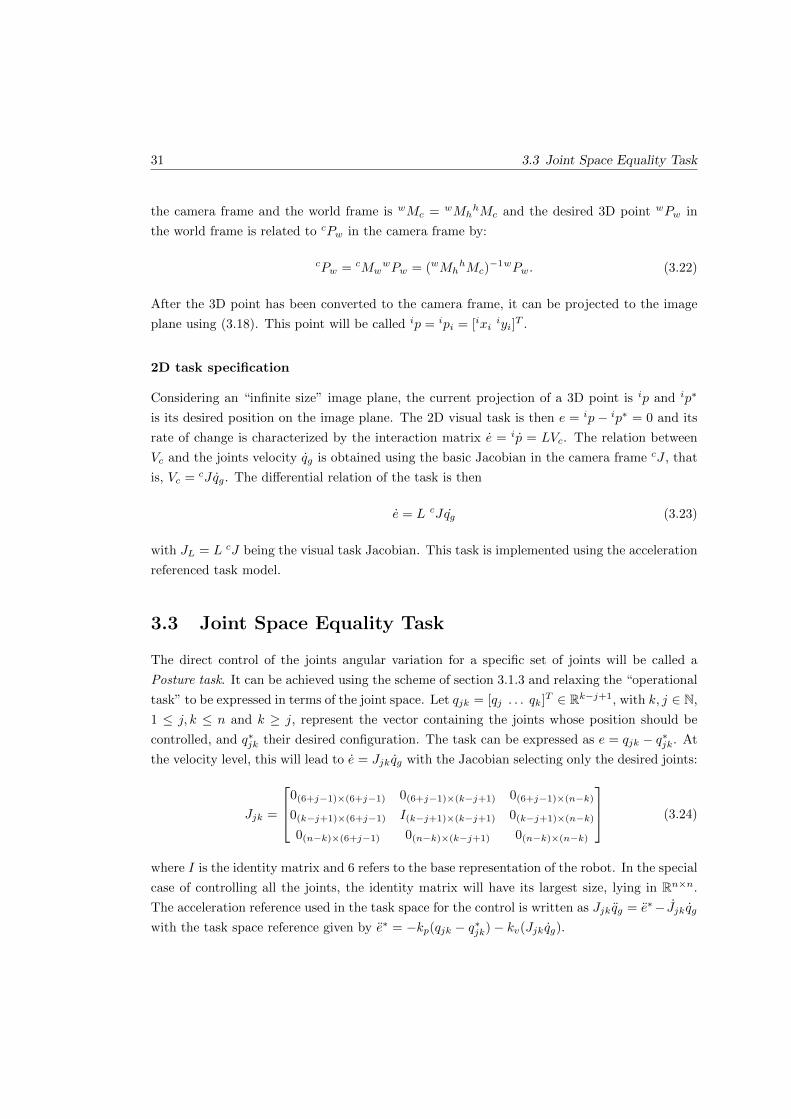
31 3.3 Joint Space Equality Task

the camera frame and the world frame is wMc = wMhhMc and the desired 3D point wPw in

the world frame is related to cPw in the camera frame by:

cPw = cMwwPw = (wMh

hMc)−1wPw. (3.22)

After the 3D point has been converted to the camera frame, it can be projected to the image

plane using (3.18). This point will be called ip = ipi = [ixiiyi]

T .

2D task specification

Considering an “infinite size” image plane, the current projection of a 3D point is ip and ip∗

is its desired position on the image plane. The 2D visual task is then e = ip− ip∗ = 0 and its

rate of change is characterized by the interaction matrix e = ip = LVc. The relation between

Vc and the joints velocity qg is obtained using the basic Jacobian in the camera frame cJ , that

is, Vc = cJqg. The differential relation of the task is then

e = L cJqg (3.23)

with JL = L cJ being the visual task Jacobian. This task is implemented using the acceleration

referenced task model.

3.3 Joint Space Equality Task

The direct control of the joints angular variation for a specific set of joints will be called a

Posture task. It can be achieved using the scheme of section 3.1.3 and relaxing the “operational

task” to be expressed in terms of the joint space. Let qjk = [qj . . . qk]T ∈ Rk−j+1, with k, j ∈ N,

1 ≤ j, k ≤ n and k ≥ j, represent the vector containing the joints whose position should be

controlled, and q∗jk their desired configuration. The task can be expressed as e = qjk − q∗jk. At

the velocity level, this will lead to e = Jjkqg with the Jacobian selecting only the desired joints:

Jjk =

0(6+j−1)×(6+j−1) 0(6+j−1)×(k−j+1) 0(6+j−1)×(n−k)

0(k−j+1)×(6+j−1) I(k−j+1)×(k−j+1) 0(k−j+1)×(n−k)

0(n−k)×(6+j−1) 0(n−k)×(k−j+1) 0(n−k)×(n−k)

(3.24)

where I is the identity matrix and 6 refers to the base representation of the robot. In the special

case of controlling all the joints, the identity matrix will have its largest size, lying in Rn×n.

The acceleration reference used in the task space for the control is written as Jjkqg = e∗− Jjkqgwith the task space reference given by e∗ = −kp(qjk − q∗jk)− kv(Jjkqg).


3.4 Inequality Task: Joint Limits

Unless the limits of the joints in position and/or orientation are explicitly included in the model

as a constraint, the output joints for the robot will be arbitrary, which would not be applicable

to the real robot which has joints restrictions due to the mechanical components. For the joint

limits task, the acceleration will be directly constrained as it will be shown in the next section.

Joint Position Limits

Each joint has a certain admissible maximum value qi and minimum value qi, and a task can

impose a restriction to make each joint satisfy these position limits. In this case, the task

vector implies all the joints directly and the task constraint is given by the double bounded

inequality q < q < q. Considering the second order approximation of q at the current time t0,

with q(t0) = q0, the restriction is written as:

q ≤ q0 + q0∆t+ q0∆t2

2≤ q (3.25)

Using (3.25), the limits for the acceleration q0 are explicitly:

qpos≤ q0 ≤ qpos (3.26)

where

qpos

=2

∆t2(q − q0 − q0∆t

)and qpos =

2

∆t2(q − q0 − q0∆t) (3.27)

The differential relation is e = Jq qg where the Jacobian excludes the coordinates corresponding

to the base of the robot and is given by

Jq =

[06×6 06×n

0n×6 In×n

](3.28)

where Jq is a particular case of (3.24) with j = 1 and k = n.

Joint Velocity Limits

In the real robot, the joints cannot be moved as fast as desired but they have velocity restric-

tions given by q in the ‘positive’ direction and q in the opposite direction. The task vector is

represented by q and the restrictions are q ≤ q ≤ q. Using the first order approximation for the

velocity at time t0, with q(t0) = q0 this restriction is:

q ≤ q0 + q0∆t ≤ q (3.29)

33 3.5 Remarks

Using (3.29), the limits for the acceleration are explicitly

qvel≤ q0 ≤ qvel (3.30)

where

qvel

=1

∆t

(q − q0

)and qvel =

1

∆t

(q − q0

)(3.31)

Since this task also works directly on each of the joints, the jacobian is also given by (3.28).

Joint and Velocity Limits

To satisfy both the position (3.26) and velocity (3.30) limits, a task has to be as restrictive as

possible and then it must consider the maximum of the lower limits and the minimum of the

upper limits for the acceleration, that is

maxqpos, qvel

≤ q ≤ min

qpos, qvel

(3.32)

This task can be also written in the following way, making clear the advantage of using the QP

solver strategy:

q ≤[Jq 0 0 0

]u ≤ q (3.33)

3.5 Remarks

In this chapter, my personal work was to adapt the classical tasks already used in the inverse-

kinematics frameworks, to inverse dynamics, specially the joint position and velocity limits, as

well as the visual-servo tasks. Using this set of basic generic tasks and constraints, the two

following chapters will present generic solutions to build a complex dynamic behavior on the

HRP-2 robot.

Chapter 4

Robot Sitting on a chair

The dynamic model and constraints described in the previous chapter were used to generate a

complex motion that deals with non-coplanar contacts and several dynamic tasks. This motion

consists in making HRP-2 N.14 (with 30 degrees of freedom) sit down in a chair using both

arms in contact with the armrests to control its down movement. Additional steps were added

to let the robot approach the chair before sitting down. Later, the same motion was extended

to the model of HRP-2 N.10, which possesses two additional degrees of freedom at the wrists.

4.1 Scenario Description

The cascade of Quadratic programming is composed as described in the previous chapter and

summarized by Figure 3.1. The tasks described here correspond to the operational task level

described in section 3.1. Even though this is a list of the tasks that were used to generate the

motion, it is not presented in a prioritized order as the tasks occur during different periods of

time and a task can have different priorities in different periods of time.

• Generic 6D tasks. The ‘acceleration referenced tasks’ were used to control the position

and orientation of the operational points at the chest, left hand, right hand, head, waist,

left foot and right foot of the robot, as shown in Figure 2.1.

• Task for the center of mass. This task controls the desired position of the Center of mass

and can be useful when performing a step in order to achieve static equilibrium, or when

sitting down in order to lower down the body.

• Visual task. It is used for the robot to move its head in such a way that the projection of

the armrest lies at the desired position in the image plane of the camera.

34

35 4.2 Sequence of Tasks

• Task for the grippers: This task is a particular case of the posture task where the joints to

be controlled are directly those corresponding to the left or right gripper. The objective

is to open or close the grippers at the armrests.

• Joint limits in velocity and position: This task is used to respect the mechanical con-

straints of the robot’s design.

Besides the tasks, the rigid contacts can be added or removed at any time. There will be

contact constraints in the feet and later in the hands when they reach the chair’s armrests so

that the robot can use them to lower down, in the same way that an old person would do it.

For each contact, a contact surface composed of four points is defined: the sole for each foot,

and the hollow of the grasp for the hands.

4.2 Sequence of Tasks

The motion sequence is the following. First, the robot moves its left leg backwards (step back),

then it turns left, looks at the armrest and moves the hand towards it in order to grasp it.

After this, the robot looks forward and then moves the right leg backwards until it is close

enough to the chair. At this moment, it looks at the right armrest and moves its right hand to

grasp it. Finally, with both hands holding the respective armrests, the robot turns its head to

face the front and sits down. This sequence is presented in Figure 4.1 indicating the tasks that

are added at a specific iteration time, with each iteration corresponding to 1 ms. The highest

priority task, after the dynamic model and the rigid contacts, is the joint limits task not shown

in the figure.

Figure 4.1: Sequence of tasks launched at every iteration for the motion with step

To perform the first step back, first the Center of mass is moved towards the foot that will

remain still, in this case the right one. Then, the motion of the swinging foot, the left one,

is composed of two parts not shown explicitly in Figure 4.1. These parts are a motion back

Chapter 4: Robot Sitting on a chair 36

and up, followed by the motion down to arrive at the same level of the supporting foot. After

the double contact, the chest is rotated to the left and then the head looks to the left using a

visual feature task, which tries to make the projection of the left armrest be located in the field

of view of the robot’s camera. At the same time, the gripper of the left hand starts opening

and the left hand starts moving to a point located just over the left armrest, which is called

pre-grasp in the figure. This pre-grasp motion is required so that the hand’s gripper can grasp

the armrest afterwards. Once it has grasped the desired armrest, the gripper closes (Cl, in the

Figure) and a rigid contact constraint is added at the left hand to ensure no further relative

motion occurs between the hand and the chair.

After adding the left contact, there are tasks in the head and chest to move straight. The

task on the head is directly applied to the head’s operational point without using a visual task

as it is not easy to define a target point at which the robot’s camera should look at. In the

meantime, the right foot moves back (up and down) without sliding. For the right armrest the

process is very similar. After grasping the right armrest and adding a rigid contact between

it and the robot’s hand, a task on the waist lowers the robot’s body down so that it can sit.

A task on the chest is added to restrict its rotation so that the chest is kept straight as the

robot’s body lowers down. At the same time, the head turns to look straight, using a task on

the head’s operational point. The experiment was performed in simulation using the model of

HRP-2 N.14, and later it was also tested using the model of HRP2 N.10; however, the results

are similar.

The task sequence to sit down without stepping back is similar to the previous paragraph

but not considering the step, as shown in Figure 4.2, where the tasks for the gripper have

been omitted. It can be observed that in this case, when the robot is sitting down, there is

no constraint on the rotation of its chest, as opposed to the previous case. Both approaches

are valid and the usage or not of more tasks to control depends on the current reaction of the

robot. Experimentation determines the possible addition of constraints.

Figure 4.2: Sequence of tasks launched at every iteration for the motion without step

As only some operational points are controlled, the motion of the other parts are left to the

dynamic model, and occasionally a physical and mathematical perfectly valid solution might

not look realistic in the sense that it would look different to the way a human would do it. In

37 4.3 Results

those cases, additional constraints can be added to obtain a motion resembling more the one

intended to be achieved, or a different approach to realize the motion can be considered. For

instance, it was experimentally verified that the center of mass is a very restrictive constraint

that can generate unwanted secondary motion if no other restrictions are imposed. When using

it to lower the body down (in order to sit), the chest and the head might bend “unnaturally”

to effectively satisfy the restriction of descending the CoM. That is why, in this experience a

waist task was used, instead, to sit down.

4.3 Results

A sequence of the described scenario of the robot sitting down is shown in Figure 4.3 and

Figure 4.4 for the case that includes an additional step back. The robot shown satisfies all the

joint position and velocity limits, which are run as the highest priority tasks. In these Figures,

t represents the iteration time corresponding to the one presented in the sequence of Figure 4.1,

which can be used to identify the tasks that the robot is performing at each iteration. Both

the frontal and lateral views correspond to the same instants of time. A video can be found

at http://homepages.laas.fr/nmansard/videos.html. The simulation environment of the figures

corresponds to the program called “robotviewer”, which is a tool developed at the Gepetto

group in LAAS-CNRS and is currently available as a Linux package.

(a) t=1 (b) t=2100 (c) t=3300

Figure 4.3: Frontal and Lateral views of the robot sitting down (part 1)


(a) t=4000 (b) t=5000 (c) t=5600

Figure 4.4: Frontal and Lateral views of the robot sitting down (part 2)

Task Errors

The temporary evolution of the task errors is expected to be exponentially decreasing since the

law e = −λe, with λ ∈ R+, was used as section 3.1.3 describes. Provided that different tasks

have different degrees of freedom in the task space, for comparison purposes the L-2 norm of

the error vector ‖e‖2 was used for Figure 4.5, which corresponds to the case that includes a

step. In Figure 4.5a, the error for the center of mass is small in magnitude compared to the

others because its initial position is close to the desired position. Both feet do not present an

exponential decay behavior because there is an intermediate desired position corresponding to

the foot floating above the ground, which was not finished but interrupted by the final position

of the foot on the ground. This interruption was done to avoid a perturbation in the robot’s

motion, specifically the motion of the non controlled joints, as no additional task on the other

operational points was imposed at that time. In these cases, the error is also small as the

desired step size and height are small.

For the hands, there is also an interruption at the middle of the motion due to the transition

between the pre-grasping and grasping tasks that modify the desired position and thus, the

current achieved error. The chest and the waist present a slow motion since the used PD

gain was small as these elements comprise much of the robot’s dynamics. Special attention is

deserved to the last error obtained with the chest, as there is a moment when the tendency of the

curve changes. This moment corresponds to an increase in the chest’s gain added to strengthen

39 4.3 Results

the control law and to show the robustness of the solver that can deal with interactive gain

changes. Figure 4.5b shows the error in the tasks that involve the motion of the head. These

tasks are the one that directly controls the operational point at the head, and the one that uses

visual features for the control. Both tasks show clearly the exponential decay behavior of the

control law. The vertical dashed lines show the iteration at which some task is added to the

stack of tasks and correspond to the iterations in Figure 4.1.

(a) Tasks corresponding to: Center of mass, hands, feet, waist and chest

(b) Tasks that move the head

Figure 4.5: Evolution of the tasks’ errors (case including step)

For the case of sitting down without performing any additional step, the temporal evolution

of the tasks is shown in Figure 4.6, which corresponds to the sequence in Figure 4.2. The same

observations of the previous graph apply to this case. The errors related to ‘look left’, ‘look

right’ and ‘look straight’ correspond to visual tasks.

Center of Mass

The temporal evolution of the Center of Mass (CoM) is shown in Figure 4.7a for the case without

steps. The Z axis presents a decrease in height by the end of the motion, which corresponds

to the moment when the robot is sitting down. It fact, irrespective of whether the CoM is

specifically controlled with a task or not, the robot will lower its center of mass when sitting

down. However, when using specifically a task on the Center of Mass the robot will try to

compensate its down motion with some co-lateral effects as the motion of the head or chest.


Figure 4.6: Evolution of the tasks’ errors (case with no step)

The projection of the Center of Mass on the ground plane (XY plane) is depicted in Fig-

ure 4.7b when there is no step. The support area for each foot is shown in solid blue lines with

the asterisk showing the projection of the operational point at the ankles. The graph is divided

in three stages and each additional contact is represented by a change in color and thickness of

the line, plus a perpendicular dash.

(a) Temporal Evolution (b) Projection on the XY (horizontal) plane

Figure 4.7: Evolution of the Center of Mass for the robot sitting without step.

The first stage corresponds to the beginning, when the only elements in contact are the

feet, with the CoM starting from the point situated in the middle of the support polygon. The

moment at which the left hand contact is added constitutes the beginning of the second stage,

and the moment of the addition of the second contact with the right hand is the third stage.

41 4.4 Remarks

During the second and third stages the contact points are no longer coplanar and the notion of

static equilibrium while the CoM remains inside the support polygon cannot be further applied.

Similarly, the classical ZMP constraint cannot be considered, since it is not defined when the

hands are in contact. In fact, after the contact with the left hand the Center of Mass starts to

leave the support polygon and by the end of the motion it is completely out, but the robot is

still stable, though. The reason for this static equilibrium is the non-coplanar contacts with the

hands that give additional support. Thus, the CoM can move more freely, sparing the degrees

of freedom to make the motion smoother and to increase the robot’s reachable space.

Joint Limits

The evolution of two particular joints is shown in Figure 4.8 with blue thin line when there are

no limits for the joint positions, and with thicker red line when the task to keep the joints inside

the limits is considered. The latter one is used throughout the experiment, but the former case

is shown only for comparison. With the joint limits task, the joint limit is reached, but not

violated thanks to the constraint (3.33), whereas without it, the limts are clearly violated.

(a) Joint at the head (b) Joint at the left hand (wrist)

Figure 4.8: Trajectory of some joints with joint limits and without joint limits

4.4 Remarks

This chapter presented the results of using the cascade control scheme on the motion generation.

The motion was generated for HRP-2 N.14 and HRP-2 N.10 using the implemented tasks

described in the previous chapter. The achieved motion was very realistic, it is dynamically


consistent, and can be directly applied on the robot. My personal contribution, at the beginning

of my Master work, was to realize the experiments and to add in the task sequences the two

initial steps that improve the realism of the motion and emphasize the dynamical performances

of the algorithm. This work was submitted to IEEE/RSJ International Conference on Intelligent

Robots and Systems IROS 2011 [54].

Chapter 5

Application of Motion Capture in

the Inverse Dynamics Control

Scheme

A motion capture system is a tool that is able to reconstruct the 3D motion of a set of marked

bodies with a high frequency and a very good accuracy (200 Hz and 1 mm in the case of

the laboratory equipment used). These bodies can constitute a bigger entity and the whole

motion can become very complex. The capture of whole-body human motion is an example

of this complexity and its imitation by a humanoid robot will be discussed in this chapter, in

particular, the imitation of the dance performed by a person. The setup described in chapter 3

will be used to reproduce a dynamically consistent motion in the robot. The contribution of this

work is to propose a complete methodology to quickly reshape a dynamic motion demonstrated

by a human expert, and adapt the dynamic of the human body to the robot body own dynamic.

5.1 Motion Capture in Robotics

The capture and analysis of motion is an active research area due to its complexity and potential

applications [39]. In robotics, it has become an active research area during these recent years [65]

to generate motion by imitation. This imitation paradigm that lets the robot acquire the way of

performing a task by observing human demonstrations has been called learning from observation

(LFO) [45] and was initially introduced for robotic manipulators with the name assembly plan

from observation (APO) [23]. Robotic applications include industrial assembly [23], humanoid

walking [38], dancing [45], yoyo playing [40] among others. Moreover, the information gathered

43

Chapter 5: Application of Motion Capture in the Inverse Dynamics Control Scheme 44

from a human motion capture system can further be organized into a database which can be

used for categorization of human behaviors based on motion, and for the synthesis of robot

motion [71].

5.1.1 Approaches

Time re-parameterization

Due to the physical limitations of a humanoid robot, the motion acquired can be slowed down

to better fit these restrictions. A time re-parametrization scheme was proposed in [65] as a

pre-processing step to account for the velocity limits of the joints. As long as ∆q∆t is larger than

the corresponding velocity limit, the time variation is increased by a fixed amount (the period)

until this constraint is satisfied. This process generates a slower motion when compared to the

original one.

Leg Task Models

One of the pioneering works for robot dancing is described in [45]. For the upper body, the

motion is directly reproduced, but for the lower body, it cannot be directly applied since the

dynamics of a person and a robot are not the same. Let to and tf represent the beginning and

ending time, respectively. The tasks defined in [45] for the legs are:

• Step: It can be applied to any leg and consists in lifting the swing foot and landing it

back, with the support foot fixed. This task is detected by analyzing the trajectory of

the foot. Let p(t) represent the position of a foot marker at time t and vp(t) be its speed.

A segment is identified as a step if it continuously presents positive speed values, i.e.:∫ tf

t0

vp(t)dt ≤ lstep, and vp(t) ≤ vstep, (t0 ≤ t ≤ tf ) (5.1)

where lstep and vstep are distance and velocity thresholds used to eliminate noise-like

motions when the foot is a support foot.

• Stand : It consists in having both feet on the ground and is assumed to be present in those

segments in which no step was detected.

• Squad : It consists in raising and lowering the waist and is detected by analyzing the

trajectory of the waist. If vh(t) is the speed of the waist, the is detected if

∫ tf

t0

|vh(t)|dt ≤ lsquat and

vh(t) < 0, t0 ≤ t ≤ tmvh(t) > 0, tm ≤ t ≤ tf

(5.2)

45 5.1 Motion Capture in Robotics

where lsquat is a threshold for the vertical moving distance that eliminates noise.

Optimization Approach

The approach to use optimization to solve the imitation problem was proposed in [65]. Let qv(t),

qr(t) be the joint positions of the upper body of the virtual actor and the robot, respectively,

q, q be the joint minimum and maximum positions, q, q be the joint minimum and maximum

velocities, Pv(t), Pr(t) be the Cartesian positions of the hands and the head of the virtual

actor and the robot, respectively, A(q(t)) be the inertia matrix of the robot, C(q(t), ˙q(t)) be

the dynamic drift (gravity torques and Coriolis accelerations), τ(t) be the vector of the applied

torques on the humanoid robot’s joints and τ , τ be torque minimum and maximum values. The

imitation problem for the upper body of the robot, considering the dynamics and the joint and

torque limits, and using X(t) = [q(t)T q(t)T q(t)T ]T as the optimization variables, is [65]:

minX(t)

∫ tf

t0

[qr(t)− qv(t)]T [qr(t)− qv(t)] + σ[Pr(t)− Pv(t)]T [Pr(t)− Pv(t)]

dt (5.3)

subject to

M(q(t))q(t) + C(q(t), q(t)) = τ(t)

q(t0) = q0, q(t0) = 0, q(t0) = 0

q(tf ) = qf , q(tf ) = 0, q(tf ) = 0

τ ≤ τ(t) ≤ τ

q ≤ ˙q(t) ≤ q

q ≤ q(t) ≤ q

where σ is a user defined constant. The solution to this problem is difficult due to the complexity

of the dynamic equation and the relation between the torques τ(t) and the joint positions q(t).

However, the problem can be transformed into a classical optimization form using Lie group and

Lie Algebra to write the recursive multi-body dynamics [49]. Using this approach, the solution

is given in terms of the Augmented Lagrange Multiplier method in [65] and a further control

of the ZMP trajectory using the cart table model [25] is applied to ensure dynamic stability.

Transition Graphs to Represent Human Motion

The information directly obtained from the motion capture system consists of a certain continu-

ous representation (usually the position) of the markers without any explicit a-priori knowledge

about when a certain type of motion starts or ends. The solution proposed by [71] is to decom-


pose the whole motion into primitives and establish the transitions between these primitives to

generate a type of motion describing a behavior. The approach consists in using the principal

component analysis (PCA) to successively cluster the motion. Let Nm be the number of mark-

ers, Nf be the number of frames, (pTim, vTim) be the position and velocity of marker m in the

frame i, and xi = [pTi1 vTi1 . . . pTiNm]T be the state vector of the i-th sample frame. In order

to cluster, each state vector xi is projected onto the eigenvector associated with the largest

eigenvalue of the autocorrelation matrix formed with xi,∀i ∈ 1, Nf. Let this 1-D projection

of vector xi be called x′i ∈ R and X ′ be the projected one dimensional dataset. The problem

is reduced to finding the threshold that minimizes the 1-D classification error. The elements of

X ′ are sorted leading to X ′s and the index th determines the division between samples th and

th + 1 using the following criteria [71]:

th = arg maxi

i log

σ1

i+ (Nf − i) log

σ2

Nf − i

(5.4)

where σ1 and σ2 represent the variance of the first i and last Nf−i elements of X ′s. This process

is repeated succesively. After the binary tree is constructed, the transition graphs between the

nodes are obtained as the ratio between the total number of transitions from node m to n and

the sum of all the transitions starting from node m.

5.2 Kinematic Application to Robot Dancing

5.2.1 Motion Capture System

The motion capture process took place at the Robotics Room at LAAS-CNRS. The system is

composed of 10 digital cameras each of them with an embedded FPGA for the signal processing,

having a resolution of 640× 480 and recording at 200 fps. The cameras are connected directly

to the tracking computer via an Ethernet connection. A set of 35 markers were placed on the

person performing the dance and the data collected from those markers was used to build a

virtual skeleton that matches the kinematic hierarchy of the robot. The number of markers is

not directly related to the number of joints in the skeleton since a subset of markers can be used

to gather robust information of a single point. In this motion capture 15 points were defined

and a total of 9674 frames were acquired.

The output obtained from the motion capture system for each node i consists of a set of 6

numbers Wm [Txi Tyi Tzi Rxi Ryi Rzi] representing the translation and rotation with respect to

the motion capture system’s reference frame that will be referred to as Wm. For the position,

cartesian coordinates (in mm) are obtained and for the orientation, roll, pitch and yaw angles

(in degrees). This output defines a coordinate system for each node. The skeleton is represented

47 5.2 Kinematic Application to Robot Dancing

Table 5.1: Segments and Nodes Hierarchy

Segment Parent node Child nodeRight Hips waist Rleg1

Right Thigh Rleg1 Rleg2Right Leg Rleg2 RfootLeft Hips waist Lleg1

Left Thigh Lleg1 Lleg2Left Leg Lleg2 Lfoot

(Same node) root waistAbdomen waist chestThorax chest head

Right Shoulder chest Rarm1Right Forearm Rarm1 Rarm2

Right Arm Rarm2 RhandLeft Shoulder chest Larm1Left Forearm Larm1 Larm2

Left Arm Larm2 Lhand

by links joining the parent and child node, as shown in Table 5.1. The waist is considered as

the root and all the segments are defined with respect to it.

5.2.2 Kinematic Optimization in Translation and Rotation

When using a motion capture system, a calibration of the components is always needed. To this

end, the person whose motion wants to be recovered starts with a position that is well known for

the robot. Using this known configuration, the transformation matrices between each node mi

and the corresponding joint qi in the robot is obtained as a “calibration” step and represented

by miTqi , which remains constant for all the process as long as the markers do not have relative

motion with respect to the body they are attached to. This matrix considers the differences in

orientation between the markers and the frames defined in the forward kinematics for each joint,

as well as the differences in segment lengths of the robot and the dancer. Another matrix that

is obtained during the calibration process is the one relating the origin of the motion capture

systme Wm and the robot’s reference frame W represented by WTWm . Let the position and

orientation of each node mi with respect to the motion capture reference frame be represented

by the homogeneous transformation WmTmi(t) which varies in time according to the motion of

the dancer. With these transformation matrices, the desired configuration of the robot’s joint

i is:WT ∗qi(t) = WTWm

WmTmi(t)miTqi (5.5)

On the other hand, the robot’s forward kinematics gives the position and orientation of each


joint qi with respect to the robot’s world reference frame W as the transformation matrixWTqi(q) which is a function of the joint vector q. Then, the problem of finding the suitable

joint values q∗(t) for the robot at a time t can be reduced to minimizing the difference between

these transformation matrices as:

q∗(t) = arg minq

n∑i

‖ WT ∗qi(t)WTqi(q) ‖2 (5.6)

s.t. qi,min ≤ qi ≤ qi,max (5.7)

where the condition to satisfy the joint limits for every joint i ∈ 1, n at every optimization

process has been added. The operator is a high level abstraction of the difference between

the matrices. Let the position and orientation part of the transformation matrices be explicitly

noted as:

WT ∗qi(t) =

[R∗qi(t) p∗qi(t)

0 1

]WTqi(q) =

[Rqi(q) pqi(q)

0 1

](5.8)

For the position part the difference to minimize is directly represented by the L − 2 norm as

‖ p∗qi(t) − pqi(q) ‖2. For the part corresponding to the orientation the difference is measured

by the the rotation angle θi about an arbitrary vector of the product Rdi = Rqi(q)R∗qi(t)

−1 ∈SO(3). If the rotation matrices are close enough, the angle of Rdi about the arbitrary vector

is very small. Representing the product of the rotation matrices as

Rdi =

nx ox ax

ny oy ay

nz oz az

(5.9)

the angle will be

θi = atan2

(√(ny − ox)2 + (nz − ax)2 + (oz − ay)2

2,nx + oy + az − 1

2

)(5.10)

which is always between 0 and π. Finally, the operator in (5.6) is given by

WT ∗qi(t)WTqi(q) = wi ‖ p∗qi(t)− pqi(q) ‖2 +(1− wi)θi (5.11)

where wi is the weight corresponding to the position part of the joint i and (1−wi) is the weight

for the orientation part. The weights are included to provide more flexibility to the model and

are experimentally determined.

49 5.2 Kinematic Application to Robot Dancing

Figure 5.1: Orientation of nodes and links

5.2.3 Virtual Skeleton Based on Joint Frames

To verify the results of the kinematic optimization process, a skeleton model that reproduces

the motion obtained form the motion capture system in the same virtual environment of the

robot was implemented. Let ni represent the i-th parent node, ni+1 its children node and li the

link joining both nodes. As figure 5.1 shows, the orientation of each node is not related to the

link that joins them, but the direction of that link can be obtained as pli = pni+1 − pni , where

p is the position with respect to the world reference frame. In the virtual environment used for

the robot, the elements are specified by their position and orientation in roll pitch yaw angles,

and even though pli represents the orientation of the link it cannot directly specify the needed

orientation angles.

To obtain these angles, a fictitious frame having its X axis coincident with the direction

of pli was introduced. Such a frame is fully described by a rotation matrix Rli ∈ SO(3)1

whose columns constitute an orthonormal basis in R3. To this end, the Gram-Schmidt process

was used. The initial basis is v1, v2, v3, with v1 = pli , and v2, v3 being random vectors.

The ortho-normalization process gives a new orthonormal basis e1, e2, e3 that can be directly

used as the columns of Rli . The first vector is directly obtained as e1 = v1‖v1‖ . For the second

vector, first u2 = v2 − (v2 · e1)e1 is obtained and then e2 = u2

‖u2‖ . For the third vector,

u3 = v3− (v3 · e1)e1− (v3 · e2)e2 and e3 = u3

‖u3‖ . Using this base, the fictitious frame describing

the link li is represented as

Tli =

[eT1 eT2 eT3 pli

o 0 0 1

](5.12)

from which the needed roll, pitch and yaw angles can be computed.

The implemented skeleton, in the same environment of the robot, is shown in Figure 5.2. It

1SO(3) constitutes the Special Orthogonal space of rotation matrices in 3D, and it is defined as SO(3) =R ∈ R3×3|RTR = I, det(R) = 1.


Figure 5.2: Robot model and the skeleton created with the motion capture data

is observed that the dimensions of the robot and the skeleton are not the same as the models

of the person and the robot do not have the same size. The skeleton shown has been built up

using directly the matrices WmTmi(t). There is an offset between the two models as the world

for the motion capture is not the same as the world for the robot. Matrix miTqi maps the joints

of the motion capture system to the ones of the robot. However, the method described in this

section can also be applied accounting for the differences between the nodes of the model and

the joints of the robot, if the matrix miTqi relating them is also considered.

5.2.4 Kinematic Results

The motion of the real dancer includes lots of head and chest rolls, which are not possible in

HRP-2 N.14 since it does not possess degrees of freedom for the roll at the head and chest.

To overcome this problem and reproduce the motion more closely, it was decided to add 2

more DOFs to the model, precisely at the head and chest; thus, the model used for the results

presented in this chapter has 32 DOF but used HRP2 N.14 as a basis. This model will be

referred to as the augmented HRP-2 N.14 model. Even though this is physically not possible

on the real HRP-2, it could be physically implemented on a robot having these capabilities, like

HRP-4, the last released robot of the HRP “family”.

The results of the kinematic optimization process in the augmented model of HRP-2 are

shown in Figure 5.3. It is noted that, since there are no contact constraints, the feet are not

restricted to stay in contact with a certain point on the ground but they can move freely to yield

a better optimization of their position and orientation and eventually “compensate” the errors

51 5.3 Dynamic Processing of the Motion

(a) (b)

Figure 5.3: Results of the kinematic optimization

in some other nodes, due to the complexity and variety of the motion. This motion on the feet

is also due to the real motion of the dancer that did some involuntary feet motion according

to the music and in some cases it is an involuntary sliding movement of the foot. Figure 5.3a

shows clearly an unwanted rotation on the left foot and Figure 5.3b shows both feet oriented

similarly among them but not properly oriented with respect to the reference frame.

5.3 Dynamic Processing of the Motion

The robot’s dynamics is different from the person’s dynamics and the motion that was recovered

using only kinematic methods, while stable on the person, is not necessarily stable on the robot.

As a result, the robot can fall down trying to follow directly the joint trajectories obtained if no

dynamic analysis is performed. Moreover, the executed dance is an example of a very dynamic

and complex motion where the arms movements can easily destabilize the robot if no dynamics

are considered. This is the reason why the motion obtained with the kinematic optimization

was further “validated” dynamically using the Cascade Scheme of chapter 3. The objective

is to reproduce the dancer’s motion and at the same time satisfy the restrictions imposed by

the dynamics of the robot. To this end, a global posture task was implemented for the robot

to follow the joint’s values, and the contact constraints with the ground were added at each

foot for the robot to satisfy the stability criteria. The stack of tasks used is the same shown

in Figure 3.1. Later, some modifications on the task space are added to better accomplish the

imitation of the dancer’s motion and eventually to include some additional movement.


5.3.1 Posture Task

The posture task introduced in section 3.3 was split into separate parts to give more freedom in

the choice of the PD gain for each part of the body. Table 5.2 shows these parts as well as the

joints implied in each one. There is an overlap between the arms and the grippers and those

Table 5.2: Joints for the posture tasks using the augmented HRP-2 model

Part JointsRight Leg 1-6Left leg 7-12Chest 13-15Head 16-18

Right Arm 19-25Left Arm 26-32

Right Gripper 25Left Gripper 32

tasks are never performed simultaneously. The task for the grippers is usually added when the

arm posture task is removed and an operational space task is executed instead. When only the

joints are to be directly followed, all the tasks presented in Table 5.2 are used, except the ones

corresponding to the grippers. Since the frequency of the motion capture system was 200 Hz

and the period used to dynamically generate the motion is 1 ms, the new desired joint values are

changed every 5 iterations and the exponential decreasing behavior is not always completed as

a new desired value appears before the previous one has been completely reached. For motion

with slow rate of change the previous and next desired values are close enough and they can

be properly followed. However, for motion with fast increments between consecutive frames,

the desired joint values are not achieved and the system acts as a low-pass filter on the joints

evolution. This is particularly noticeable when there are oscillations, like the arm moving up

and down consecutively or the knees moving continuously forward and backward.

5.3.2 Addition of Arbitrary Tasks

The posture task reproduces the desired motion at the joint level satisfying the dynamic con-

straints but the system acts as a low-pass filter generating problems specially for the fast

oscillatory motion. Nevertheless, the structure of the stack of tasks can be profited to overcome

this problem since tasks on operational points can be added and removed at any time and the

priorities can also be modified. To this end, at a certain moment an operational task can be

added to enhance or even modify the original motion of the dancer. There are two cases:

• Specification of target points. A new desired point in the operational space can be spec-

53 5.3 Dynamic Processing of the Motion

ified without defining the desired trajectory to reach it. This point can be determined

recovering the position of the operational point obtained with the kinematic optimization

or it can be arbitrarily set.

• Specification of a trajectory. Let the trajectory for the operational point x obtained with

the kinematic optimization be called xo(t). The new trajectory xn(t) that will be set as the

desired trajectory for that operational point will be given by xn(t) = xo(t)+xm(t), where

xm(t) is a trajectory modification that can be done in any of the six degrees of freedom

of x. This trajectory modification xm(t) can be time varying or constant, according to

the needs.

It is important to point out that the operational task added must have a higher priority than

the joints posture task it would interfere with. For instance, if an operational task is added to

the hand, the priority of the arm’s posture task must be lowered or removed, but it is preferred

to be kept, as it will serve as a “guide for the new trajectory. If this priority considerations

are not taken into account, the desired motion would be binded by the solutions to the posture

task with higher priority and the desired effect would not be achieved.

5.3.3 Foot Sliding

To let a foot slide, the rigid contact constraints in (2.6) can be relaxed constraining the motion

to the XY plane. For the contact i, this restriction at the velocity level can be formulated as

vz = 0, ωx = 0, ωy = 0 allowing the other velocity elements to take arbitrary values. This

guarantees no translation on the Z axis or rotation about it. To account for this constraints,

the dynamic model would need to be reformulated. Alternatively, another simpler and more

flexible approach is to remove the contact constraint and add a task that restricts the motion

in Z. Considering x∗ as the desired task, this particular case of the 6D task is

x∗ =

kx

ky

Hz

0

0

krz

Sx =

0 0 0 0 0 0

0 0 0 0 0 0

0 0 1 0 0 0

0 0 0 1 0 0

0 0 0 0 1 0

0 0 0 0 0 0

(5.13)

where Sx is the selection matrix defined in section 3.2.1, kx, ky, krz ∈ R are arbitrary values

and Hz is the known height of the operational point at the foot with respect to the world when

the foot is in contact with the ground. This constraint restricts the height of the foot to remain

constant, and the rotation about the X and Y axis to be null.


5.4 Results

5.4.1 Operational Space Modifications

As presented in section 5.3.2, the stack of tasks makes it possible to add operational tasks to

correct the motion. Even though there were also modifications in the left hand, left knee and

waist, in this section only the results corresponding to the right hand and the right knee will

be presented as the other cases are similar.

Right Hand

This task was added to better move the arm up and down and it is an example of trajectory

specification. The changes obtained for the right hand are shown in Figure 5.4. As observed,

the hand has been moved to a higher position using an operational task.

(a) Without Task space correction (b) With Task space correction

Figure 5.4: Modification of the hand position adding an operational task

Case of the Knees

The knees constitute a particular case as the dancer permanently moved them but at the

dynamic level this motion was not so evident. To correct this problem using the task approach,

the motion of the joint that comprises the knee was analyzed. Figure 5.5a shows the joint

evolution obtained after the kinematic optimization for the right knee. Between iterations 2000

and 2800, and between 6200 and 7300, the motion of the joint is oscillatory and those are the

moments corresponding directly to the observed motion at the dancer’s right knee. A scalogram

using the Gaussian wavelet was constructed and is shown in Figure 5.5, where it is observed

(in red circle) that there are salient frequencies at those points. It was determined that the

scale a corresponding to the maximum values at the desired positions is 36. The frequency and

55 5.4 Results

(a)

(b)

Figure 5.5: Scalogram of the right knee’s joint evolution

the scales are related by f =fsfwa

, where fs is the sampling frequency and fw is the center

frequency of the wavelet [1]. For the Gaussian derivative of order 4, fc = 0.5, and considering

that the sampling period used during the acquisition is 200 Hz, the resulting frequency is 2.7

Hz. Then, a task on the knee was added at that frequency to resemble more the motion.

Figure 5.6a shows the evolution of the joint at the right knee (joint number 4) in the joint

space as a function of the iteration number, and Figure 5.6b shows the evolution in the X axis

of the operational space. Note that there is a difference in the iteration time of Figure 5.5 and

Figure 5.6 as the former one corresponds to the kinematic optimization of the motion sampled

at 200Hz and the latter corresponds to the dynamic level that runs at 1000Hz (1000 iterations

correspond to 1 second of motion). The red line shows the evolution of the joint when there

is only the posture task in the leg, and the blue line shows the evolution when the operational

task is added to the knee, but both lines are obtained using the dynamic control scheme. Even

though the joint is not directly controlled, it is observed in Figure 5.6a that with the operational

task addition, the joint at the knee presents an oscillation with higher amplitude, whereas with

only the task posture the oscillation is weak. Also, a similar evolution pattern is shown. The

results in the X axis of the operational space show a clear consistent oscillation with similar

amplitude in the two places where the knees motion was added. Both the joint space and the

operational space show the effect of the task at the knee.


(a) Joint Space (joint number 4)

(b) Task Space (X axis)

Figure 5.6: Temporal evolution of the Right knee

5.4.2 Whole Body Motion Result

The results of the whole body motion after the dynamic processing are shown in Figure 5.7

(and a video is available at http://homepages.laas.fr/nmansard/videos.html). It is observed

that the feet remain in a constant position due to the rigid contacts constraint imposed in the

dynamic model. However, by the end of the motion there is an intended sliding on the foot as

described in section 5.3.3.

5.5 Remarks

The contribution of this chapter is the novel approach for motion imitation using the dynamic

control scheme. Several posture tasks constituted the backbone in the motion generation. A

new approach for fast motion edition or correction was presented using operational space tasks

with higher priority than the posture tasks corresponding to the involved parts of the body.

Using these methods, any type of motion acquired using a motion capture system can be

imitated and the results are guaranteed to be dynamically stable.

57 5.5 Remarks

(a) (b) (c)

(d) (e) (f)

(g) (h) (i)

(j) (k) (l)

Figure 5.7: Results for the whole boby motion of the robot imitating the dance

Chapter 6

Conclusions and Future Work

A method for generating whole-body motion of humanoid robots, i.e. highly redundant robots in

rigid contact with their environment, has been discussed. The method allows to build complex

dynamic behaviors, based on a composition of tasks and constraints that are used as basic

bricks for motion generation. Several tasks have been proposed and implemented. Two cases

have been presented to validate the model. The first case is the robot sitting down in a chair.

The second one is the imitation of the dynamic motion performed by a human.

The generation of the motion was based on an existing, but very novel and still in devel-

opment, dynamic control scheme that allows the prioritization of tasks as well as the addition

or removal of contact constraints. Several tasks were added to this scheme in order to gen-

erate the motion. The control of each operational point corresponding to a certain part of

the body was performed using operational 6D (position and orientation) tasks selecting only

the necessary degrees of freedom. A visual task was integrated into the dynamic scheme, as

well as several posture tasks to directly follow the joints desired behavior for each part of the

body. This posture split gives more freedom for the assignation of different gains to each part,

and facilitates the addition of operational tasks to modify the motion of a certain part of the

body. Similarly, the joint limits in velocity, as well as their integration with the joint position

limits, were introduced as constraints. This set of tasks allows to build an entire motion by

specifying “by hand” the initial and final points of each task. Compared to the methods that

require the specification of the motion of each joint, the programing by task sequencing is a

huge simplification.

Redundancy posed several problems to the generation of motion. The problem of achieving a

certain reference (for example, the specified position and orientation) with a task (for example,

the operational point) is solved thanks to redundancy. However, the problem of satisfying

the task making the motion natural is difficult due to redundancy: a task can be effectively

58

59

achieved but it might not resemble the way a human would do it. Even though redundancy

makes it possible for the robot to realize different tasks with its different parts simultaneously,

it has been experienced that it poses great difficulties when trying to achieve a desired motion

as the generated behaviors were sometimes unpredictable. This is the reason why special

considerations were taken when specifying the desired positions and orientations: “collateral

motion” can be generated in the non-controlled parts of the body due to the interaction between

tasks. The most representative case found was the task on the center of mass that produces

some unwanted side motion, and the solution was to constraint the parts of the body that

presented that motion. However, there is currently no a-priory solution to achieve the desired

motion without the trial and error phase. Future work might deal with this problem: the

realization of tasks automatically satisfying constraints so that the motion can achieve human-

like appearance.

For complex and long motion, the anthropomorphism of the robot can be profited to simplify

the motion design by using the motion capture system, which gives a good basis of the motion

to realize. The motion of a human dancer was recovered from a motion capture system and

the joints were obtained using optimization on the forward kinematics model. This kinematic

reshaping is what is classically done when relying on motion capture for editing a motion for a

robot or for an avatar, but the motion thus obtained is only kinematic: it is not dynamically

consistent. The kinematic motion was successfully integrated to the dynamic control scheme

to satisfy the dynamic constraints under the assumption that the feet remained fixed on the

ground. However, due to the various filters used during the data processing and dynamic

reshaping, some flaws appear during the imitation. Moreover, the difference between the real

demonstration and the kinematic model, including the assumptions used for reshaping, posed

problems during the kinematic optimization phase, and later, to the dynamic processing phase.

These problems were solved at the level of the dynamic solver with the addition of arbitrary

tasks that locally correct the robot motion and make it more similar to the desired one. These

corrections show the powerfulness of the dynamic control scheme, which lets the movements

obtained from the motion capture system be dynamically consistent in a short period of time,

as opposed to other approaches to robot dancing that spent even years dealing with the robot

stability.

The method described for imitation of robot dancing can be, in general, applied to the

imitation of any type of motion. The obtained motion is dynamically consistent, and could be

directly applied on the real humanoid robot. However, this validation is still to be performed,

and is the most exciting perspective of this work. In particular, this would require to reshape

the motion for the real 30-DOF HRP-2 model (since an augmented robot model was used to

better follow the dancer motion) that has less capabilities for imitation of a dance or other

types of motion.

Chapter 6: Conclusions and Future Work 60

The quantitative evaluation of the results is complicated as, being the main objective to

make the motion realistic, there exists no ground truth to compare with. The only possible

measurement is the rate of change of the error for each task, which is desired to present an

exponential decay behavior. But even when those task errors have the desired temporal evolu-

tion, the generated motion can be by far different to the expected one and they serve only as a

formalism to verify that the tasks are being achieved and that the whole system is mathemati-

cally correct; which does not imply any guarantee of good results from the motion appearance

perspective. The only means for the evaluation of the generated motion is the visual inspection

in the simulator. For the same reason, it is complicated to quantitatively compare our results

with other works, as there are no indicators of motion quality.

Future work would consider the extension of the dynamic model to deal with other cases of

contact constraints, like foot sliding (in this work foot sliding was achieved but as a special case

of an operational task). The stability conditions can be also extended to walking on slopes and

uneven terrain. A further extension using the data obtained with the motion capture system

would be to study the human motion in order to recover the tasks that constitute it, analyzing

the possibly existing natural restrictions imposed by the human way of doing the things rather

than by the physical constraints. In sum, there is a lot of work to do regarding whole-body

human motion.

Appendix A

Generalized Inverses

A.1 Generalized Inverse

Let A be a matrix in Rm×n. A generalized inverse of A is a matrix A# ∈ Rn×m satisfying

AA#A = A. A reflexive generalized inverse of A is a matrix A#r ∈ Rn×m satisfying AA#

r A = A

and A#r AA

#r = A#

r [7], [6].

In the general case, A# and A#r are not unique. Given a generalized inverse, A#, of A, all the

generalized inverses of A matrices are given by A#g = A# +Z−A#AZAA#, where Z ∈ Rn×m is

an arbitrary matrix. Since every pseudoinverse A+ is also a generalized inverse, and is uniquely

defined as shown in the following section, it can be used to compute all the generalized inverses.

Properties

1. ∀A ∈ Rm×n ∃A#, ρ(A#) ≥ ρ(A).

2. A# = A#r ⇔ ρ(A#) = ρ(A).

3. AA# = (AA#)2 and A#A = (A#A)2.

4. If A is square and nonsingular, then, A# and A#r are unique and A# = A#

r = A−1.

5. Let the sets of A#, A#r , A+ be S#, S#

r , S+, respectively, then, S+ ⊂ S#r ⊂ S#.

A.2 Pseudoinverse

The pseudoinverse (sometimes also called the Moore-Penrose inverse) of a matrix A ∈ Rm×n

is a matrix A+ ∈ Rn×m satisfying the so called Penrose conditions [51], which are AA+A = A,

61

Chapter A: Generalized Inverses 62

A+AA+ = A+, (AA+)T = AA+ and (A+A)T = A+A.

The pseudoinverse A+ of A is obtained in the following way:

• if A ∈ Rm×n, m < n and ρ(A) = m, then AAT is nonsingular and A+ = AT (AAT )−1,

• if A ∈ Rm×n, n < m and ρ(A) = n, then ATA is nonsingular and A+ = (ATA)−1AT ,

• if A ∈ Rn×n and ρ(A) = n, then A+ = A−1,

where ρ(A) represents the rank of matrix A.

Properties

1. ∀A ∈ Rm×n, A+ is unique.

2. (A+)+ = A.

3. (AT )+ = (A+)T .

4. A+ = (ATA)+AT = AT (AAT )+.

5. The following matrices are symmetric and idempotent: A+A, AA+, I−A+A and I−AA+.

6. If A = AT ∈ Rn×n and A2 = A, then ∀B ∈ Rm×n, A(BA)+ = (BA)+.

Relation with Linear Equations

Let A ∈ Rm×n, x ∈ Rn and y ∈ Rm. For a linear equation Ax = y, the general form of the

least-squares solutions minimizes the error norm, that is, min ‖ y − Ax ‖2, and is given by

x = A+y+ (I −A+A)z, where z ∈ Rn is an arbitrary vector. The minimum norm solution also

satisfies the optimization min ‖ x ‖2 and is given by x = A+y.

A.3 Weighted Generalized-Inverse

Let A be a matrix in Rm×n, and R, L be positive definite matrices. The generalized inverse

of matrix A weighted on the right by R and on the left by L is the matrix AL#R satisfying

AAL#RA = A, AL#RAAL#R = AL#R [6], [14]. This weighted inverse is given by:

AL#R =√R(√LA√R)+√L (A.1)

where the matrices√R or

√L can be computed using the Cholesky decomposition. The problem

Ax = b is solved with x = AL#Rb as

min‖x‖R, x = argmin‖Ax− b‖L. (A.2)

63 A.3 Weighted Generalized-Inverse

If A−1 exists, then AL#R = A−1. The generalized inverse of matrix A weighted on the right

by R is:

A#R =√R(A√R)+ = RAT (ARAT )+ (A.3)

and the generalized inverse of matrix A weighted on the left by L is:

AL# = (√LA)+

√L = (ATLA)+ATL. (A.4)

There are two particular cases depending on the rank of A:

A is full row-rank

In this case, an additional property is (RA#RA)T = RA#RA, and the weighted generalized-

inverses are given by

A#R = RAT (ARAT )−1 (A.5)

AL# = A+ (A.6)

A is full column-rank

In this case, an additional property is (LAAL#)T = LAAL#, and the weighted generalized-

inverses are given by

A#R = A+ (A.7)

AL# = (ATLA)−1ATL (A.8)

Remark about Notation

Even though the notation for the generalized inverse, pseudoinverse and weighted generalized-

inverse used in this appendix is very common, there is no standard notation referring to these

concepts. The signs A#, A+, A− or A† are not standard, and in different works they might

refer to either the pseudoinverse or the generalized inverse. Even more, sometimes the terms

generalized inverse and pseudoinverse are used in a swapped way. As long as the terms are clear

from the concept this is accepted. However, throughout this thesis, the notation presented in

this appendix is used.

Appendix B

Optimization Approach for

General Linear Systems

B.1 Equality and Inequality Systems

Let A ∈ Rm×n, b ∈ Rm, C ∈ Rp×n and d ∈ Rp. The general problem of finding x ∈ Rn given

systems of m linear equalities and p linear inequalities:

Ax = b (B.1)

Cx ≤ d (B.2)

is equivalent to the following minimization problem [28]:

minx∈Ω,w∈Rp

1

2‖Ax− b‖2 +

1

2‖w‖2 (B.3)

with

Cx− d ≤ w (B.4)

where Ω is a non-empty convex subset of Rn and w plays the role of a slack variable. The set

Sop of optimal solutions to (B.3) is convex and non-empty, and it can be shown that all the

optimal solutions satisfy a same set of inequalities and violate the others by a same amount [28].

Note that an inequality in both sides like d ≤ Cx ≤ d can be reduced to the form of (B.2) as

C ′x ≤ d′ with C ′ = [C − C]T ∈ R2p×n and d′ = [d − d]T ∈ R2p

and can be solved using (B.3), (B.4). A linear equality can also be considered as an inequality

bounded in both sides where both bounds are equal: b ≤ A ≤ b, which is equivalent to (B.1).

64

65 B.2 Prioritization of Linear Systems

B.2 Prioritization of Linear Systems

Let a system be composed of p priority levels, where the lower the number of the level, the

more priority it has. At each level k let the linear systems of equalities and inequalities be

represented by Ak, bk, Ck, dk as in (B.1) and (B.2). The objective is to satisfy the higher

priority levels and then, the lower priority levels, if possible, without interfering with the higher

priority ones. To this end, the following scheme is proposed in [28]:

S0 = Rn (B.5)

Sk = arg minx∈Sk−1,w∈Rp

1

2‖Akx− bk‖2 +

1

2‖w‖2

(B.6)

with Ckx− dk ≤ w (B.7)

where at level k the variable x is constrained to be in the optimal subset of the previous priority

solution Sk−1, and thus, it can be shown that Sk ⊆ Sk−1 and that, if Sk−1 is a non-empty convex

set, Sk will also be a non-empty convex set. This equation is solved iteratively starting with

the highest priority and descending to the lower priorities sequentially, as in the algorithm

proposed in [28]. An alternative notation for this process [15] at level k considering double

bounded inequalities dk ≤ Ckxk ≤ dk is

minxk,wk

1

2‖wk‖2 (B.8)

dk ≤ Ckxk − wk ≤ dk (B.9)

dak−1 ≤ Cak−1xk − w∗k−1 ≤ da

k−1 (B.10)

where Cak−1 = [C1 . . . Ck−1]T , dak−1 = [d1 . . . dk−1]T , da

k−1 = [d1 . . . dk−1]T , w∗k−1 is a

fixed value obtained at the previous priority level k − 1 and the final x is x = xnt with nt

being the total number of tasks. In case of conflicts between the constraints, the slack variable

wk allows to violate the current constraints (at level k) giving priority to the constraints at

the previous levels k − 1. In that case, this variable measures the amount of violation that is

minimized as much as possible by (B.8). Note that the equalities are not explicitly included as

Akxk = bk can be written as bk ≤ Akxk ≤ bk. For single bounded inequalities, the restriction

for the unbounded side is set to ∞ or −∞ according to the case. The prioritization process is

then regarded as a simple Quadratic Program (QP) with linear constraints that can be solved

efficiently.

Bibliography

[1] P. Abry. Ondelettes et turbulence multiresolutions. Algorithmes De Decomposition, In-

variance Dechelles, 1997.

[2] T. Arakawa and T. Fukuda. Natural motion generation of biped locomotion robot using

hierarchical trajectory generation method consisting of ga, ep layers. In Robotics and

Automation, 1997. Proceedings., 1997 IEEE International Conference on, volume 1, pages

211–216. IEEE, 1997.

[3] P. Baerlocher and R. Boulic. Task-priority formulations for the kinematic control of highly

redundant articulated structures. In Intelligent Robots and Systems, 1998. Proceedings.,

1998 IEEE/RSJ International Conference on, volume 1, pages 323–329. IEEE, 1998.

[4] P. Baerlocher and R. Boulic. An inverse kinematics architecture enforcing an arbitrary

number of strict priority levels. The visual computer, 20(6):402–417, 2004.

[5] J. Baillieul. Kinematic programming alternatives for redundant manipulators. In Robotics

and Automation. Proceedings. 1985 IEEE International Conference on, volume 2, pages

722–728. IEEE, 1985.

[6] A. Ben-Israel and T.N.E. Greville. Generalized inverses: Theory and applications. Springer

Verlag, 2003.

[7] T.L. Boullion and P.L. Odell. Generalized inverse matrices. Wiley-interscience, 1971.

[8] S.R. Buss. Introduction to inverse kinematics with jacobian transpose, pseudoinverse and

damped least squares methods. University of California, San Diego, Typeset manuscript,

available from http://math. ucsd. edu/˜ sbuss/ResearchWeb, 2004.

[9] Y.H. Chang, Y. Oh, D. Kim, and S. Hong. Balance control in whole body coordination

framework for biped humanoid robot MAHRU-R. In Robot and Human Interactive Com-

munication, 2008. RO-MAN 2008. The 17th IEEE International Symposium on, pages

401–406. IEEE, 2008.

66

67 BIBLIOGRAPHY

[10] F. Chaumette and S. Hutchinson. Visual servo control. I. Basic approaches. Robotics &

Automation Magazine, IEEE, 13(4):82–90, 2006.

[11] S. Chiaverini. Singularity-robust task-priority redundancy resolution for real-time kine-

matic control of robot manipulators. Robotics and Automation, IEEE Transactions on,

13(3):398–410, 1997.

[12] J.J. Craig. Introduction to Robotics: Mechanics and Control. 2005.

[13] J. Denavit and RS Hartenberg. A kinematic notation for lower-pair mechanisms based on

matrices. Trans. ASME J. Appl. Mech, 22(1):215–221, 1955.

[14] K.L. Doty, C. Melchiorri, and C. Bonivento. A theory of generalized inverses applied to

robotics. The International Journal of Robotics Research, 12(1):1, 1993.

[15] A. Escande, N. Mansard, and P.B. Wieber. Fast resolution of hierarchized inverse kine-

matics with inequality constraints. In Robotics and Automation (ICRA), 2010 IEEE In-

ternational Conference on, pages 3733–3738. IEEE, 2010.

[16] R. Featherstone and D. Orin. Robot dynamics: Equations and algorithms. In Robotics and

Automation, 2000. Proceedings. ICRA’00. IEEE International Conference on, volume 1,

pages 826–834. IEEE, 2000.

[17] L. Geppert. Qrio, the robot that could. IEEE Spectrum, 41(5):34–37, 2004.

[18] A. Goswami. Foot rotation indicator (fri) point: A new gait planning tool to evaluate

postural stability of biped robots. In Robotics and Automation, 1999. Proceedings. 1999

IEEE International Conference on, volume 1, pages 47–52. IEEE, 1999.

[19] D. Gouaillier, V. Hugel, P. Blazevic, C. Kilner, J. Monceaux, P. Lafourcade, B. Marnier,

J. Serre, and B. Maisonnier. Mechatronic design of NAO humanoid. In Robotics and

Automation, 2009. ICRA’09. IEEE International Conference on, pages 769–774. IEEE,

2009.

[20] H. Hanafusa, T. Yoshikawa, and Y. Nakamura. Analysis and control of articulated robot

with redundancy. In IFAC, 8th Triennal World Congress, volume 4, pages 1927–1932,

1981.

[21] K. Hirai, M. Hirose, Y. Haikawa, and T. Takenaka. The development of Honda humanoid

robot. In Robotics and Automation, 1998. Proceedings. 1998 IEEE International Confer-

ence on, volume 2, pages 1321–1326. IEEE, 1998.

BIBLIOGRAPHY 68

[22] R. Hirose and T. Takenaka. Development of the humanoid robot ASIMO. Honda R&D

Technical Review, 13(1):1–6, 2001.

[23] K. Ikeuchi and T. Suehiro. Toward an assembly plan from observation. Task recognition

with polyhedral objects. Robotics and Automation, IEEE Transactions on, 10(3):368–385,

1994.

[24] S. Kajita, H. Hirukawa, K. Harada, and K. Yokoi. Introduction a la commande des robots

humanoıdes: de la modelisation a la: generation du mouvement. Springer, 2009.

[25] S. Kajita, F. Kanehiro, K. Kaneko, K. Fujiwara, K. Harada, K. Yokoi, and H. Hirukawa.

Biped walking pattern generation by using preview control of zero-moment point. In

Robotics and Automation, 2003. Proceedings. ICRA’03. IEEE International Conference

on, volume 2, pages 1620–1626. Ieee, 2003.

[26] K. Kaneko, F. Kanehiro, S. Kajita, H. Hirukawa, T. Kawasaki, M. Hirata, K. Akachi, and

T. Isozumi. Humanoid robot HRP-2. In Robotics and Automation, 2004. Proceedings.

ICRA’04. 2004 IEEE International Conference on, volume 2, pages 1083–1090. IEEE,

2004.

[27] K. Kaneko, F. Kanehiro, M. Morisawa, K. Miura, S. Nakaoka, and S. Kajita. Cybernetic

human HRP-4C. In Humanoid Robots, 2009. Humanoids 2009. 9th IEEE-RAS Interna-

tional Conference on, pages 7–14. IEEE, 2009.

[28] O. Kanoun, F. Lamiraux, P.B. Wieber, F. Kanehiro, E. Yoshida, and J.P. Laumond.

Prioritizing linear equality and inequality systems: application to local motion planning

for redundant robots. In Robotics and Automation, 2009. ICRA’09. IEEE International

Conference on, pages 2939–2944. IEEE, 2009.

[29] I. Kato, Y. Mori, and T. Masuda. Pneumatically powered artificial legs walking automat-

ically under various circumstances. In Proceedings of the 4th International Conference on

External Control of Human Extremities, pages 458–470, 1972.

[30] O. Khatib. Commande dynamique dans l’espace operationnel des robots manipulateurs

en presence d’obstacles. Docteur Ingenieur Thesis, L’Ecole Nationale Superieure de

l’Aeronautique et de l’Espace, 1980.

[31] O. Khatib. Real-time obstacle avoidance for manipulators and mobile robots. The inter-

national journal of robotics research, 5(1):90, 1986.

[32] O. Khatib. A unified approach for motion and force control of robot manipulators: The

operational space formulation. IEEE Journal of robotics and automation, 3(1):43–53, 1987.

69 BIBLIOGRAPHY

[33] O. Khatib, L. Sentis, J. Park, and J. Warren. Whole body dynamic behavior and control

of human-like robots. International Journal of Humanoid Robotics, 1(1):29–43, 2004.

[34] Y. Kusuda. Toyota’s violin-playing robot. Industrial Robot: An International Journal,

35(6):504–506, 2008.

[35] N. Mansard and F. Chaumette. Task sequencing for high-level sensor-based control.

Robotics, IEEE Transactions on, 23(1):60–72, 2007.

[36] N. Mansard, O. Stasse, P. Evrard, and A. Kheddar. A versatile generalized inverted

kinematics implementation for collaborative working humanoid robots: The stack of tasks.

In Advanced Robotics, 2009. ICAR 2009. International Conference on, pages 1–6. IEEE,

2009.

[37] G. Metta, L. Natale, F. Nori, G. Sandini, D. Vernon, L. Fadiga, C. von Hofsten,

K. Rosander, M. Lopes, J. Santos-Victor, et al. The iCub humanoid robot: An open-

systems platform for research in cognitive development. Neural Networks, 23(8-9):1125–

1134, 2010.

[38] K. Miura, M. Morisawa, S. Nakaoka, F. Kanehiro, K. Harada, K. Kaneko, and S. Kajita.

Robot motion remix based on motion capture data towards human-like locomotion of hu-

manoid robots. In Humanoid Robots, 2009. Humanoids 2009. 9th IEEE-RAS International

Conference on, pages 596–603. IEEE, 2009.

[39] T.B. Moeslund, A. Hilton, and V. Kruger. A survey of advances in vision-based human

motion capture and analysis. Computer vision and image understanding, 104(2-3):90–126,

2006.

[40] K. Mombaur and M.N. Sreenivasa. HRP-2 plays the yoyo: From human to humanoid

yoyo playing using optimal control. In Robotics and Automation (ICRA), 2010 IEEE

International Conference on, pages 3369–3376. IEEE, 2010.

[41] R.M. Murray, Z. Li, and S.S. Sastry. A mathematical introduction to robotic manipulation.

CRC, 1994.

[42] Y. Nakamura. Advanced robotics: redundancy and optimization. Addison-Wesley Longman

Publishing Co., Inc. Boston, MA, USA, 1990.

[43] Y. Nakamura, H. Hanafusa, and T. Yoshikawa. Task-priority based redundancy control of

robot manipulators. The International Journal of Robotics Research, 6(2):3, 1987.

BIBLIOGRAPHY 70

[44] J. Nakanishi, R. Cory, M. Mistry, J. Peters, and S. Schaal. Operational space control:

A theoretical and empirical comparison. The International Journal of Robotics Research,

27(6):737, 2008.

[45] S. Nakaoka, A. Nakazawa, F. Kanehiro, K. Kaneko, M. Morisawa, H. Hirukawa, and

K. Ikeuchi. Learning from observation paradigm: Leg task models for enabling a biped

humanoid robot to imitate human dances. The International Journal of Robotics Research,

26(8):829, 2007.

[46] K. Nishiwaki, J. Kuffner, S. Kagami, M. Inaba, and H. Inoue. The experimental humanoid

robot H7: a research platform for autonomous behaviour. Philosophical Transactions of

the Royal Society A: Mathematical, Physical and Engineering Sciences, 365(1850):79, 2007.

[47] Y. Ogura, H. Aikawa, K. Shimomura, A. Morishima, H. Lim, and A. Takanishi. Devel-

opment of a new humanoid robot WABIAN-2. In Robotics and Automation, 2006. ICRA

2006. Proceedings 2006 IEEE International Conference on, pages 76–81. IEEE, 2006.

[48] J.H. Oh, D. Hanson, W.S. Kim, Y. Han, J.Y. Kim, and I.W. Park. Design of android

type humanoid robot Albert HUBO. In Intelligent Robots and Systems, 2006 IEEE/RSJ


[49] F.C. Park, J.E. Bobrow, and SR Ploen. A Lie group formulation of robot dynamics. The

International journal of robotics research, 14(6):609, 1995.

[50] I.W. Park, J.Y. Kim, J. Lee, and J.H. Oh. Mechanical design of humanoid robot platform

KHR-3 (KAIST humanoid robot 3: HUBO). In Humanoid Robots, 2005 5th IEEE-RAS


[51] R. Penrose. A generalized inverse for matrices. In Mathematical proceedings of the Cam-

bridge philosophical society, volume 51, pages 406–413. Cambridge Univ Press, 1955.

[52] D. Raunhardt and R. Boulic. Progressive clamping. In Robotics and Automation, 2007

IEEE International Conference on, pages 4414–4419. IEEE.

[53] L. Saab, N. Mansard, F. Keith, JY Fourquet, and P. Soueres. Generation of Dynamic Mo-

tion for Anthropomorphic Systems under Prioritized Equality and Inequality Constraints.

In Robotics and Automation, 2011. Proceedings. ICRA’11. 2011 IEEE International Con-

ference on. IEEE, 2011.

[54] L. Saab, O. Ramos, N. Mansard, P. Soueres, and J-Y. Fourquet. Generic Dynamic Motion

Generation with Multiple Unilateral Constraints. In Intelligent Robots and Systems, 2011

IEEE/RSJ International Conference on ”submitted”. IEEE, 2011.

71 BIBLIOGRAPHY

[55] J. Salvi, X. Armangue, and J. Batlle. A comparative review of camera calibrating methods

with accuracy evaluation* 1. Pattern recognition, 35(7):1617–1635, 2002.

[56] C. Samson, B. Espiau, and M.L. Borgne. Robot control: the task function approach. Oxford

University Press, 1991.

[57] L. Sciavicco and B. Siciliano. A solution algorithm to the inverse kinematic problem for

redundant manipulators. Robotics and Automation, IEEE Journal of, 4(4):403–410, 1988.

[58] L. Sentis. Synthesis and control of whole-body behaviors in humanoid systems. PhD thesis,

Stanford University, CA, USA, July 2007.

[59] L. Sentis and O. Khatib. Control of free-floating humanoid robots through task priori-

tization. In Robotics and Automation, 2005. ICRA 2005. Proceedings of the 2005 IEEE


[60] J. Shan and F. Nagashima. Neural locomotion controller design and implementation for

humanoid robot HOAP-1. In 20th Annual Conference of the Robotics Society of Japan,

2002.

[61] B. Siciliano, L. Sciavicco, and L. Villani. Robotics: modelling, planning and control.

Springer Verlag, 2009.

[62] B. Siciliano and J.J.E. Slotine. A general framework for managing multiple tasks in highly

redundant robotic systems. In Advanced Robotics, 1991.’Robots in Unstructured Environ-

ments’, 91 ICAR., Fifth International Conference on, pages 1211–1216. IEEE, 1991.

[63] M.W. Spong, S. Hutchinson, and M. Vidyasagar. Robot modeling and control. John Wiley

& Sons, 2006.

[64] S. Sugano and I. Kato. WABOT-2: Autonomous robot with dexterous finger-arm–Finger-

arm coordination control in keyboard performance. In Robotics and Automation. Proceed-

ings. 1987 IEEE International Conference on, volume 4, pages 90–97. IEEE, 1987.

[65] W. Suleiman, E. Yoshida, F. Kanehiro, J.P. Laumond, and A. Monin. On human motion

imitation by humanoid robot. In Robotics and Automation, 2008. ICRA 2008. IEEE


[66] R. Tellez, F. Ferro, S. Garcia, E. Gomez, E. Jorge, D. Mora, D. Pinyol, J. Oliver, O. Torres,

J. Velazquez, et al. Reem-B: An autonomous lightweight human-size humanoid robot. In

Proc. IEEE-RAS Int. Conf. Humanoid Robot.(Humanoids, pages 462–8, 2008.

BIBLIOGRAPHY 72

[67] M. Vukobratovic and B. Borovac. Zero-moment point-thirty five years of its life. Interna-

tional Journal of Humanoid Robotics, 1(1):157–173, 2004.

[68] M. Vukobratovic and D. Juricic. Contribution to the synthesis of biped gait. Biomedical

Engineering, IEEE Transactions on, (1):1–6, 1969.

[69] D.E. Whitney. The mathematics of coordinated control of prosthetic arms and manipula-

tors. Journal of Dynamic Systems, Measurement, and Control, 94:303, 1972.

[70] K. Yamane and Y. Nakamura. Dynamics filter-concept and implementation of online

motion generator for human figures. Robotics and Automation, IEEE Transactions on,

19(3):421–432, 2003.

[71] K. Yamane, Y. Yamaguchi, and Y. Nakamura. Human motion database with a binary tree

and node transition graphs. Autonomous Robots, 30(1):87–98, 2011.

generation of complex dynamic motion for a humanoid...

Documents