1

Generation of Synthetic Spatially EmbeddedPower Grid Networks

Saleh Soltan and Gil Zussman

Abstract—The development of algorithms for enhancing theresilience and efficiency of the power grid requires performanceevaluation with real topologies of power transmission networks.However, due to security reasons, such topologies and particularlythe locations of the substations and the lines are usually not publiclyavailable. Therefore, we study the structural properties of theNorth American grids and present an algorithm for generatingsynthetic spatially embedded networks with similar properties toa given grid. The algorithm uses the Gaussian Mixture Model(GMM) for density estimation of the node positions and generatesa set of nodes with similar spatial distribution to the nodes in agiven network. Then, it uses two procedures, which are inspiredby the historical evolution of the grids, to connect the nodes. Thealgorithm has several tunable parameters that allow generatinggrids similar to any given grid. Particularly, we apply it to theWestern Interconnection (WI) and to grids that operate under theSERC Reliability Corporation (SERC) and the Florida ReliabilityCoordinating Council (FRCC), and show that it generates gridswith similar structural and spatial properties to these grids. Tothe best of our knowledge, this is the first attempt to considerthe spatial distribution of the nodes and lines and its importancein generating synthetic power grids.

Index Terms—Power Grids, Structural Properties, SyntheticNetworks, Spatial Networks, Data Mining.

I. INTRODUCTION

The design of algorithms and methods for enhancing thepower grid (namely, making it smarter) drew tremendousattention over the past decade [1], [2]. These efforts focusedon challenges stemming from renewable generation intercon-nection [3], Phasor Measurement Units (PMUs) placement[4], [5], transmission expansion planning [6], and vulnerabilityanalysis [7], [8], [9], [10]. The development of algorithms forcoping with these challenges requires performance evaluationwith real grid topologies. However, in order to avoid exposingvulnerabilities, the topologies of the power transmission net-works and particularly the locations of the substations and thelines are usually not publicly available or are hard to obtain.

There are only very few and limited test cases and real-world power grid datasets that are publicly and freely avail-able. These include the IEEE test cases [11], the NationalGrid UK [12], the Polish grid [13], and an approximate modelof the European interconnected system [14]. To the best ofour knowledge, among these, National Grid UK is the onlypublicly available dataset with geographical locations. Evenif the data was available, it would be unwise to publishvulnerability results which are based on real topologies, due tothe enormous cost of grid enhancements. On the other hand, it

S. Soltan and G. Zussman are with the Department of Electrical Engineer-ing, Columbia University, New York, NY, 10027.E-mail: {saleh,gil}@ee.columbia.edu

Fig. 1: The North American Electric Reliability Corpora-tion (NERC) regional entities and the National ElectricityTransmission Grid of Mexico (NETGM). Different reliabilitycorporations/councils are marked with different colors.

was recently shown that simple random graph models cannotbe used to generate grids with appropriate structural andspatial characteristics [15] (for more details, see Section II).Therefore, in this paper we design an algorithm for generatingsynthetic networks with similar structural and spatial proper-ties to real power grids. Such synthetic networks can be usedfor evaluation of various methods and techniques.

To demonstrate the algorithm design and to evaluate itsperformance, we focus on the transmission networks of theNorth American and Mexican power grids (see NERC andNETGM in Fig. 1) using data that we obtained from thePlatts Geographic Information System (GIS) [16]. We con-sider one of the two major interconnections – the WesternInterconnection (WI) (see Fig. 2) which includes the WesternElectricity Coordinating Council in the United States (WECC)and Canada (WECCC) (see Fig. 1 for their coverage areas).Moreover, we consider two regional entities that operate underthe Eastern Interconnection (EI) which is the other majorinterconnection – the SERC Reliability Corporation (SERC),which is as large as the WI, and the Florida ReliabilityCoordinating Council (FRCC), which is much smaller thanthe WI. To the best of our knowledge, this is the first timethat the entire dataset of the North American and Mexicangrids as well as those of SERC and FRCC are processed andanalyzed1.

For the entire North American and Mexican grid as well asfor WI, SERC, and FRCC, we consider four metrics that cap-ture the networks’ structural properties: average path length,

1Partial analysis of the WI dataset has been conducted before – see SectionII.

arX

iv:1

508.

0444

7v1

[cs

.SY

] 1

8 A

ug 2

015

2

Fig. 2: The Western Interconnection (WI) power grid with14,302 substations (nodes) and 18,769 lines (edges).

clustering coefficient, degree distribution of the nodes, and thelength distribution of the lines. The first three metrics are verycommon [15], [17], [18], [19], [20], [21], [22]. However, tothe best of our knowledge, the length distributions of the lineshave not been thoroughly studied before. These distributionsare particularly important, since the physical properties of aline (e.g., admittance and type) are directly correlated with itslength [23], and hence, the distributions directly impact theperformance of various algorithms.

Motivated by the results of the structural properties’ analy-sis, we present the Geographical Network Learner and Gener-ator (GNLG) Algorithm for generating a network with similarproperties to a given grid. First, using Gaussian MixtureModel (GMM), the algorithm estimates the density of thenode positions and uses the obtained parameters to generatea set of nodes with a similar spatial distribution to thesenodes (the algorithm uses the Bayesian Information Criterion(BIC) to find the best number of clusters for the GMM).Then, the GNLG Algorithm uses two procedures, which areinspired by the historical evolution of power grids, to connectthe generated nodes. Particularly, since the two main designconsiderations of the grid are connectivity and robustness, thealgorithm obtains a spanning tree of the nodes to provideconnectivity and then adds more edges to the network graphto increase its robustness. The addition of edges is tuned tocreate a synthetic network with properties that are similar tothose of a given network.

To evaluate the performance of the GNLG Algorithm,we use it to generate networks similar to the WI, SERC,and FRCC. We show that by adapting a number of tunableparameters, the GNLG Algorithm can generate synthetic net-works with similar structural and spatial properties to thesepower grid networks. Overall, we believe that by adaptingthe algorithm’s tunable parameters, it is possible to generatesynthetic networks similar to any given power grid network.

This paper is organized as follows. Section II reviewsrelated work. Section III describes the dataset and the metrics,and presents the metrics for the different grids. Section IV

describes the GNLG Algorithm and Section V numericallyevaluates its performance. We conclude and discuss futureresearch directions in Section VI.

II. RELATED WORK

The structural properties of various power grids (e.g., inNorth America, some European countries, and Iran) werestudied in [17], [21], [24], [25], [26], [27]. Most of thesestudies considered one or two properties (e.g., average degree,degree distribution, average path length, and clustering coef-ficient) and computed it in a given power grid. In some cases(e.g., [15], [17], [18], [19], [20], [21], [22]) a certain classof graphs was suggested as a good representative of a powergrid network, based on one or two structural properties. Forexample, Watts and Strogatz [17] suggested the small-worldgraph as a good representative, based on the shortest pathlengths between nodes and the clustering coefficient of thenodes. Barabasi and Albert [18] showed that scale-free graphsare better representatives based on the degree distribution.However, by comparing the WI with these models, Cotilla-Sanchez, et al. [15] showed that none of them can representthe WI properly.

More detailed models that are specifically tailored to thepower grid characteristics were proposed in [28], [29] but theydid not consider the nodes’ spatial distribution and the lengthdistribution of the lines. The spatial distribution of the nodesis correlated with the length of the lines, and as mentionedabove, it is important to consider line lengths when designinga method for synthetic power grid generation. While thereare several models for generating spatial networks [30], [31],[32], most of them were not designed to generate networkswith properties similar to power grid networks. To the best ofour knowledge, this paper is the first to consider the spatialdistribution of the nodes in power grids and its importance ingenerating synthetic networks with similar structural proper-ties.

III. PRELIMINARIES AND STRUCTURAL PROPERTIES

In this section, we study the structural properties of theentire North American and Mexican grid (denoted by NA&M)as well as of the WI, SERC, and FRCC grids. We obtainedthe data from the Platts GIS [16] and conducted longitude-latitude to planar (x, y) coordinate transformation, using thegreat-circle distance method. Since the files containing sub-stations and files containing lines are not always consistent,we extracted the coordinates of the substations from the endpoint coordinates of the lines. We then used the geographicalcoordinates of the substations and the lines to construct thegraphs with nodes and edges that represent substations andlines, respectively. We used the map of reliability coorpo-rations/councils boundaries to divide the graph into regionalentities (as in Fig. 1). To the best of our knowledge, beside [7],[8] where an approximation of the WI graph was extractedfrom the Platts GIS dataset for simulations, it is the first timethat this dataset is processed and analyzed.

In addition to the number of the nodes and edges, we usefour metrics for classifying the structural properties of these

3

0.0 0.5 1.0 1.5 2.0 2.5 3.0 3.5

−11

−9

−7

−5

−3

−1

Log degree

Log

dens

ity

(a) NA&M

0.0 0.5 1.0 1.5 2.0 2.5 3.0 3.5

−11

−9

−7

−5

−3

−1

Log degree

Log

dens

ity

(b) WI

0.0 0.5 1.0 1.5 2.0 2.5 3.0 3.5

−11

−9

−7

−5

−3

−1

Log degree

Log

dens

ity

(c) SERC

0.0 0.5 1.0 1.5 2.0 2.5 3.0 3.5

−11

−9

−7

−5

−3

−1

Log degree

Log

dens

ity

(d) FRCC

Fig. 3: The degree distribution of the nodes in the NA&M, WI, SERC, and FRCC grids (in log-log scale). Linear regressionlines with slopes ζ = −4.28, ζ = −3.48, ζ = −3.93, and ζ = −2.76, respectively, are fitted to the tail distribution of thedegrees.

TABLE I: Summary of the structural properties of the NA&M,WI, SERC, and FRCC grids.

Network NA&M WI SERC FRCCNumber of Nodes (n) 55,231 14,302 12,946 1,312Number of Edges (m) 70,088 18,769 16,658 1,780Average Path Length (L) 26.66 17.33 19.71 11.68Clustering Coefficient (C) 0.049 0.049 0.049 0.075Degree Distribution (ζ) -4.28 -3.48 -3.93 -2.76

networks: average path length, clustering coefficient, degreedistribution of the nodes, and length distribution of the lines.Table I includes these metrics for the NA&M, WI, SERC, andFRCC grids.Notation. We denote the WI, SERC, and FRCC power gridtransmission networks by graphs GWI , GSERC , and GFRCC ,respectively. For each network, n and m denote the numberof the nodes and edges. di denotes the degree of node i andpi ∈ R2 denotes its position. We define ρ as the averageEuclidean distance of a node from its N nearest neighbors.We use the prime symbol (′) to denote the values for agenerated network (e.g., G′WI denotes the generated network).All the logarithms in this paper are natural logarithms. All thegeographical distances in this paper are Euclidean distances(i.e., ‖pi − pj‖2 is the distance between nodes i and j).

A. Average path length

The average path length, denoted by L, is one of thecommon metrics used for classifying graphs. It is defined asthe number of edges in the shortest path between two nodes,averaged over all pairs of vertices:

L =1

n(n− 1)

∑i6=ji,j∈V

dist(i, j),

where dist(i, j) is the number of edges in the shortest pathbetween nodes i, j. As can be seen in Table I, the averagepath length in all the four networks is in O(log(n)) which isvery small and suggests that these networks have the small-world property.

B. Clustering coefficient

An important metric is the clustering coefficient, denotedby C and defined as follows. For each node i, with degree di

at most di(di − 1)/2 edges can exist between its neighborsN(i). Let Ci denotes the fraction of these allowable edgesthat actually exist:

Ci =|{{r, s}|r, s ∈ N(i), {r, s} ∈ E}|

di(di − 1)/2.

Then, averaging Ci over all the nodes: C =∑i∈V Ci/n. As

can be seen in Table I, the clustering coefficient for all thefour networks is very small.

C. Degree distribution of the nodes

The degree distribution of the nodes is another importantmetric for classifying graphs (e.g., scale-free networks). Fig. 3shows the degree distribution of the nodes in the NA&M, WI,SERC, and FRCC grids in log-log scale. The degree one nodesin these networks usually correspond to power plants or smalltowns. These figures may suggest that the tail of the degreedistribution follows a power-law distribution in all the threenetworks. However, following [33] and since these networksare finite, we do not have enough statistical evidence to supportthe power-law hypothesis. Therefore, we only use the slope (ζ)of the fitted linear regression line to the tail distribution forcomparison purposes.

In Section V, we use the Kolmogrov-Smirnov (KS) statis-tic [34] to compare the degree distribution of the nodes in agiven network and a generated network. If P (x) and Q(x)are two Cumulative Distribution Functions (CDFs), the KSstatistic between these two is defined as follows:

DKS = maxx|P (x)−Q(x)|.

D. Length distribution of the lines

As mentioned above, the length distribution of the lines isone of the important parameters that needs to be sustainedin synthetic power grid generation. Fig. 4 shows the lengthdistribution of the lines in the NA&M, WI, SERC, and FRCCgrids. The length distribution of the lines in the NA&M grid

4

Log length

Den

sity

−6 −4 −2 0 2 4 6 8

0.0

0.1

0.2

0.3

0.4

(a) NA&MLog length

Den

sity

−6 −4 −2 0 2 4 6 8

0.0

0.1

0.2

0.3

0.4

(b) WILog length

Den

sity

−6 −4 −2 0 2 4 6 8

0.0

0.1

0.2

0.3

0.4

(c) SERCLog length

Den

sity

−6 −4 −2 0 2 4 6 8

0.0

0.1

0.2

0.3

0.4

(d) FRCC

Fig. 4: The distributions of the actual line lengths (in km) in the NA&M, WI, SERC, and FRCC grids (the lengths’ statisticsappear in Table II). Nonparametric distribution fits to the log length distributions are shown in blue.

−4 −2 0 2 4 6

−8

−6

−4

−2

Log length

Log

dens

ity

Fig. 5: The distribution of the actual line lengths (in km) inthe NA&M grid in log-log scale. A linear regression line withslope −1.61 is fitted to the tail distribution of the lengths.

TABLE II: Statistics of the actual line lengths in the NA&M,WI, SERC, and FRCC grids and of the corresponding straightlines (Euclidean distances) between substations in those grids(in km). The statistics of the straight lines are shown in thegrey cells.

Network NA&M WI SERC FRCC

Mean 15.46 16.63 13.29 12.8214.30 15.78 11.39 9.95

Standard Deviation 32.55 43.91 22.29 20.1430.68 40.78 17.90 15.6

Maximum 1,714.82 1,714.82 795.44 282.741,380.35 1,380.35 409.92 226.25

in log-log scale is shown in Fig. 5.2 The lengths’ statisticsappear in Table II.

The line lengths in Figs. 4 and 5 are the actual lengths ofthe power lines (these lines are not necessarily straight linesbetween two substation). To enable the comparison betweenthe length distributions of the lines in the real and generatednetworks, in Section V we use the point-to-point Euclideandistances to represent the line lengths in the real and thegenerated networks. Table II includes the statistics regardingboth the actual line lengths and the lengths of the straightlines between the substations, in order to demonstrate thedifferences between the metrics.

In Section V, we use Kullback-Leibler (KL) divergence

2As can be seen in Figs. 4 and 5, there are some very short lines (≈ 30m)in the considered networks. We checked the dataset to verify the credibilityof these lines and did not find any issues (these lines are categorized as below230kV lines).

Algorithm 1: Geographical Network Learner and Gener-ator (GNLG)

Input: G, {pi}ni=1, and parameters κ, α, β, γ > 0 and N ∈ N.1: Generate a set of nodes with similar spatial distribution to the nodes

in G using the SDNG Procedure (Subsection IV-A).2: Connect the generated nodes using the TWST Procedure

(Subsection IV-B).3: Add more edges to the generated graph using the

Reinforcement Procedure (Subsection IV-B).4: return the generated graph G′.

to measure the similarity between the length distribution ofthe lines in a given network and a generated network. TheKL-divergence is a non-symmetric measure of the differencebetween two probability distribution functions p and q. Specif-ically, the KL-divergence of q from p, denoted DKL(p‖q), is ameasure of the information lost when q is used to approximatep:

DKL(p‖q) =

∫ ∞−∞

p(x) lnp(x)

q(x)dx.

To estimate the KL-divergence between distributions, we usethe FNN library in R which utilizes the method introducedin [35] for estimating the KL-divergence between two distri-butions using their samples.

IV. GENERATING A SYNTHETIC NETWORK

In this section, we introduce the Geographical NetworkLearner and Generator (GNLG) Algorithm (Algorithm 1) forgenerating a synthetic network similar to a given network.The algorithm uses the Gaussian Mixture Model (GMM) fordensity estimation of the node positions and generates a set ofnodes with similar spatial distribution to the nodes in a givennetwork (the SDNG Procedure described in Subsection IV-A).Then, it connects the nodes using two procedures whosedesign principles are inspired by historical evolution of thegrids (the TWST and Reinforcement procedures described inSubsection IV-B). The GNLG Algorithm can be applied to anynetwork, where the important part is tuning the parameters toa given network. In the following subsections, we describethe building blocks of the GNLG Algorithm and use the WIto demonstrate the algorithm design and operation. Then, inSection V, we evaluate the algorithm using the WI, SERC,and FRCC grids.

5

Procedure 1: Spatially Distributed Nodes Generator(SDNG)

Input: G, {pi}ni=1.1: Fit a GMM model to {pi}ni=1 to cluster them into c clusters that

maximizes the BIC.2: For all i = 1, . . . , n sample zi from the categorical probability

distribution π obtained from GMM.3: For all i sample p′i from the probability distribution N (µzi ,Σzi )

obtained from GMM.4: return {p′i}ni=1.

A. Node positions

We now introduce the Spatially Distributed Nodes Genera-tor (SDNG) Procedure (Procedure 1) for generating a set ofnodes with similar spatial distribution to the nodes in a givennetwork. The node positions are correlated with the populationand geographical properties (e.g., Fig. 2). Thus, the nodes canbe clustered into groups based on their geographical proximity.Mixture models and in particular Gaussian Mixture Models(GMM) are commonly used for clustering and density esti-mation [36]. Hence, the SDNG Procedure uses the GMM forclustering the positions and uses BIC to find the best number ofclusters (c). It obtains the mean and covariance matrix (µj ,Σj)of the points in clusters j = 1, . . . , c along with the categoricalprobability of the clusters π = (π1, . . . , πc). Then, it uses theseparameters to generate n nodes with similar spatial distributionas the nodes in a given network.

For implementing the SDNG Procedure, we used themclust library in R [37] to apply GMM to our dataset. Thislibrary uses the Expectation Maximization (EM) algorithm tofit a GMM and provides the Bayesian Information Criterion(BIC) for the selected number of clusters. Clustering the nodesin the WI into 55 clusters results in the maximum BIC. Hence,the SDNG Algorithm clusters WI into c = 55 clusters. Ascan be seen in Fig. 7, the distribution of the generated nodesappears very similar to the distribution of the nodes in the WI.

Notice that for a given network, step 1 in the Procedureshould be executed only once. Then, having the fitted GMMparameters, the procedure can be used to generate severalinstances of nodes with similar spatial distribution to the nodesin the given network. Hence, once the parameters are available,synthetic grids can be generated with no need to access thereal grid data.

B. Connections between the nodes

We introduce two procedures (steps 2 and 3 in the GNLGAlgorithm) for connecting the generated nodes. Their designis inspired by the historical evolution of power grids. Thetwo main design consideration of the grid are (i) connectivityand (ii) robustness. Therefore, we first present the TunableWeight Spanning Tree (TWST) Procedure for finding a span-ning tree and to ensure connectivity. We then describe theReinforcement Procedure for adding more edges and ensuringthe network robustness as well as for tuning the structuralproperties of the synthetic network to resemble those of agiven network.

1) Connectivity: In order for the power grid to operate,the substations (nodes) should be connected. Due to con-struction costs, in the real world new substations are usually

Fig. 6: An example of clustering the nodes in the WI into 10clusters using GMM.

Fig. 7: A set of nodes, that were generated using the SDNGProcedure, with a similar spatial distribution to the nodes inthe WI.

connected to the nearest substation in the existing grid. Sincethe power grids have evolved gradually and locally, they donot necessarily contain the Minimum weight Spanning Tree(MST) of the nodes in the plane (the weight of a spanningtree T = (VT , ET ) is the sum of the edge lengths in T :WT =

∑{i,j}∈ET ‖p

′i − p′j‖). Hence, we do not focus on

finding the MST. Instead, we present the TWST Procedure(Procedure 2), which imitates the the gradual grid evolution.It is a low complexity procedure for finding a spanning treewith a tunable weight.

The procedure uses the average node location, denoted by:p′ =

∑i p′i/n. It first orders the nodes in n rounds (see

step 2) to obtain a permutation of indices σ : {1, 2, . . . , n} →{1, 2, . . . , n}. At round i, it samples a node j from the nodesthat were not already sampled with probability proportional to‖p′j − p′‖−κ, where κ is a parameter. It then sets σ(i) ← j.In step 5 it connects each node σ(i) to its nearest neighborσ(j∗) such that j∗ < i.

The procedure results in a tree whose weight highly dependson the ordering of the nodes, and thereby on κ. Moreover, there

6

κ

Wei

ght o

f the

Spa

nnin

g Tr

ee

150

170

190

0 2 4 6 8

127

141κ = ∞

MST

(a)

0 2 4 6 8

2045

7095

120

κ

Ave

rage

Pat

h Le

ngth

150 κ = ∞

(b)

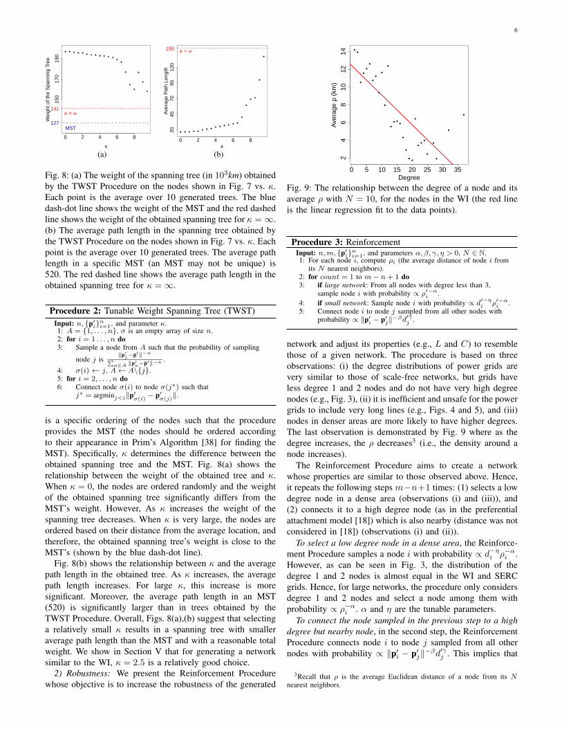
Fig. 8: (a) The weight of the spanning tree (in 103km) obtainedby the TWST Procedure on the nodes shown in Fig. 7 vs. κ.Each point is the average over 10 generated trees. The bluedash-dot line shows the weight of the MST and the red dashedline shows the weight of the obtained spanning tree for κ =∞.(b) The average path length in the spanning tree obtained bythe TWST Procedure on the nodes shown in Fig. 7 vs. κ. Eachpoint is the average over 10 generated trees. The average pathlength in a specific MST (an MST may not be unique) is520. The red dashed line shows the average path length in theobtained spanning tree for κ =∞.

Procedure 2: Tunable Weight Spanning Tree (TWST)Input: n, {p′i}ni=1, and parameter κ.1: A = {1, . . . , n}, σ is an empty array of size n.2: for i = 1 . . . , n do3: Sample a node from A such that the probability of sampling

node j is‖p′j−p′‖−κ∑a∈A ‖p′a−p′‖−κ .

4: σ(i) ← j, A← A\{j}.5: for i = 2, . . . , n do6: Connect node σ(i) to node σ(j∗) such that

j∗ = argminj<i‖p′σ(i)− p′

σ(j)‖.

is a specific ordering of the nodes such that the procedureprovides the MST (the nodes should be ordered accordingto their appearance in Prim’s Algorithm [38] for finding theMST). Specifically, κ determines the difference between theobtained spanning tree and the MST. Fig. 8(a) shows therelationship between the weight of the obtained tree and κ.When κ = 0, the nodes are ordered randomly and the weightof the obtained spanning tree significantly differs from theMST’s weight. However, As κ increases the weight of thespanning tree decreases. When κ is very large, the nodes areordered based on their distance from the average location, andtherefore, the obtained spanning tree’s weight is close to theMST’s (shown by the blue dash-dot line).

Fig. 8(b) shows the relationship between κ and the averagepath length in the obtained tree. As κ increases, the averagepath length increases. For large κ, this increase is moresignificant. Moreover, the average path length in an MST(520) is significantly larger than in trees obtained by theTWST Procedure. Overall, Figs. 8(a),(b) suggest that selectinga relatively small κ results in a spanning tree with smalleraverage path length than the MST and with a reasonable totalweight. We show in Section V that for generating a networksimilar to the WI, κ = 2.5 is a relatively good choice.

2) Robustness: We present the Reinforcement Procedurewhose objective is to increase the robustness of the generated

0 5 10 15 20 25 30 35

24

68

1012

14

Degree

Ave

rage

ρ (

km)

Fig. 9: The relationship between the degree of a node and itsaverage ρ with N = 10, for the nodes in the WI (the red lineis the linear regression fit to the data points).

Procedure 3: ReinforcementInput: n,m, {p′i}ni=1, and parameters α, β, γ, η > 0, N ∈ N.1: For each node i, compute ρi (the average distance of node i from

its N nearest neighbors).2: for count = 1 to m− n+ 1 do3: if large network: From all nodes with degree less than 3,

sample node i with probability ∝ ρ′−αi .4: if small network: Sample node i with probability ∝ d′−ηi ρ′−αi .5: Connect node i to node j sampled from all other nodes with

probability ∝ ‖p′i − p′j‖−βd′γj .

network and adjust its properties (e.g., L and C) to resemblethose of a given network. The procedure is based on threeobservations: (i) the degree distributions of power grids arevery similar to those of scale-free networks, but grids haveless degree 1 and 2 nodes and do not have very high degreenodes (e.g., Fig. 3), (ii) it is inefficient and unsafe for the powergrids to include very long lines (e.g., Figs. 4 and 5), and (iii)nodes in denser areas are more likely to have higher degrees.The last observation is demonstrated by Fig. 9 where as thedegree increases, the ρ decreases3 (i.e., the density around anode increases).

The Reinforcement Procedure aims to create a networkwhose properties are similar to those observed above. Hence,it repeats the following steps m−n+1 times: (1) selects a lowdegree node in a dense area (observations (i) and (iii)), and(2) connects it to a high degree node (as in the preferentialattachment model [18]) which is also nearby (distance was notconsidered in [18]) (observations (i) and (ii)).

To select a low degree node in a dense area, the Reinforce-ment Procedure samples a node i with probability ∝ d−ηi ρ−αi .However, as can be seen in Fig. 3, the distribution of thedegree 1 and 2 nodes is almost equal in the WI and SERCgrids. Hence, for large networks, the procedure only considersdegree 1 and 2 nodes and select a node among them withprobability ∝ ρ−αi . α and η are the tunable parameters.

To connect the node sampled in the previous step to a highdegree but nearby node, in the second step, the ReinforcementProcedure connects node i to node j sampled from all othernodes with probability ∝ ‖p′i − p′j‖−βd

′γj . This implies that

3Recall that ρ is the average Euclidean distance of a node from its Nnearest neighbors.

7

Fig. 10: A network with 14,302 nodes and 18,769 edgesgenerated based on the WI grid using the GNLG Algorithmwith κ = 2.5, α = 1, β = 3.2, γ = 2.5, and N = 10.

node i preferentially connects to a high-degree node, unlessthe high-degree node is too far in which case it is desirable toconnect to a low-degree but nearby node. This is very similarto the model introduced in [31], [32]. However, here we onlyuse these probabilities for sampling and do not use them forconnecting every pair of nodes.

We note that β determines the length distribution of thenew lines and γ determines the likelihood of the existenceof high degree nodes. If β is large compared to γ, thennew edges connect nearby nodes, thereby resulting in a largeclustering coefficient and a large average path length. If γ islarge compared to β, then new edges connect nodes to highdegree nodes regardless of their distance, thereby resulting invery high degree nodes and long edges. Hence, there should bea balance between the β and γ values. We show in Section Vthat for generating a network similar to the WI, β = 3.2 andγ = 2.5 are relatively good choices.

V. EVALUATION

In this section, we use the GNLG Algorithm to generatenetworks similar to the WI, SERC, and FRCC grids. Weevaluate the structural properties of the obtained networks andshow that they have similar properties to the real networks.

A. WI

As mentioned in Section IV-B, the parameters κ, α, β, γ,Ncan be used to tune the structural properties of the obtainednetwork. Therefore, we conducted several numerical experi-ments in which the parameters were adapted and the structuralproperties were evaluated. We observed empirically that thefollowing parameters values provide a network with similarproperties to the WI: κ = 2.5, α = 1, β = 3.2, γ = 2.5, andN = 10. Moreover, as mentioned in Section IV-A, BIC wasused to determine the number of clusters (c = 55).

The nodes generated by the SDNG Procedure were shownin Fig. 7. The network obtained by the GNLG Algorithmappears in Fig. 10 and visually resembles the WI. To study the

0.0 0.5 1.0 1.5 2.0 2.5 3.0 3.5

−8

−6

−4

−2

Log degree

Log

dens

ity

(a) GWI

0.0 0.5 1.0 1.5 2.0 2.5 3.0 3.5

−8

−6

−4

−2

Log degree

Log

dens

ity

(b) G′WI

Fig. 11: The degree distribution of the nodes in GWI andG′WI (in log-log scale). Linear regression lines with slopesζ = −3.48 and ζ = −3.99 are fitted to the distributionsof the nodes with degree greater that 2 in GWI and G′WI ,respectively. The KS statistic between the degree distributionsis 0.047.

Log length

Den

sity

−6 −4 −2 0 2 4 6 8

0.00

0.10

0.20

0.30

(a) GWI

Log length

Den

sity

−6 −4 −2 0 2 4 6 8

0.00

0.10

0.20

0.30

(b) G′WI

Fig. 12: The length (in km) distribution of the point-to-point lines in GWI and G′WI and nonparametric distributionfit (shown in blue). The KL-divergence between the lengthdistributions in GWI and G′WI is 0.14.

structural similarity between the obtained network G′WI andthe GWI , we evaluated G′WI based on the metrics describedin Section III. The clustering coefficient and the averagepath length of G′WI are C ′ = 0.052 and L′ = 17.40,respectively, and are very close to those of GWI (C = 0.049and L = 17.33).

Fig. 11 shows the degree distribution of the nodes in G′WI .As can be seen, the slope of the fitted regression line to the tailof the distribution is −3.99 which is similar to that of GWI

(−3.4). Moreover, the KS statistic between the cumulativedegree distributions in GWI and G′WI is 0.047, indicatingthe similarity between the degree distributions. Fig. 12 showsthe length distribution of the lines in G′WI . Since the GNLGAlgorithm uses straight lines to connect the nodes, we comparethe length distribution of the lines in G′WI with the lengthdistribution of the straight point-to-point lines in GWI . TheKL-divergence between the length distributions of the lines inGWI and G′WI is DKL = 0.14, indicating that distributionsare similar.

Table III summarizes the structural properties of the GWI

and five instances generated by the GNLG Algorithm. Theresults indicate that the Algorithm can generate syntheticnetworks with similar structural properties to the WI grid.

8

TABLE III: Comparison between the structural properties ofWI (GWI ) and the Generated WI (G′WI ). Five instances ofG′WI are shown to illustrate that the metric values are similar.All networks have 14,302 nodes and 18,769 edges.

Networks L C ζ DKS DKLGWI 17.33 0.049 -3.48 0 0G′WI 17.40 0.052 -3.99 0.047 0.14G′WI(2) 18.36 0.052 -3.65 0.050 0.15G′WI(3) 18.36 0.049 -3.99 0.047 0.12G′WI(4) 19.06 0.052 -3.61 0.049 0.14G′WI(5) 17.79 0.051 -3.50 0.049 0.14

Fig. 13: A part of the Eastern Interconnection (EI) with 12,946substations (nodes) and 16,658 lines (edges) that operatesunder the SERC.

B. SERC

We apply the GNLG Algorithm to part of the EI thatoperates under the SERC (see Fig. 13) that has 13,602substations (nodes) and 17,767 lines (edges) . Fig. 14 showsthe obtained network using the GNLG Algorithm with κ = 3,α = 0.5, β = 3.2, γ = 2.5, and N = 5 that are selectedempirically following several numerical experiments. In theSDNG Procedure, SERC has been clustered into c = 50clusters based on the BIC.

The comparison between the degree distribution of thenodes and the length distributions of the lines in GSERC andG′SERC are shown in Figs. 15 and 16. Table IV, summarizesthe structural properties of GSERC and five instances gen-erated by the GNLG Algorithm. As with the WI, it can beseen that the Algorithm can generate synthetic networks withsimilar structural properties to the SERC grid.

C. FRCC

Finally, we apply the GNLG Algorithm to a smaller part ofthe EI with 1,312 substations (nodes) and 1,780 lines (edges)that operates under the FRCC (see Fig. 17). As can be seenin Fig. 18, the degree distribution of the nodes in GFRCC isdifferent from the degree distribution of the nodes in GWI

and GSERC . In GFRCC , only the density of the nodes withdegree 1 is not on the fitted regression line. This suggests thatin the Reinforcement Procedure, the step for small networks

Fig. 14: A network with 12,946 nodes and 16,658 edgesgenerated based on the SERC grid using the GNLG Algorithmwith κ = 3, α = 0.5, β = 3.2, γ = 2.5, and N = 5.

0.0 0.5 1.0 1.5 2.0 2.5 3.0

−8

−6

−4

−2

Log degree

Log

dens

ity

(a) GSERC

0.0 0.5 1.0 1.5 2.0 2.5 3.0

−8

−6

−4

−2

Log degree

Log

dens

ity(b) G′SERC

Fig. 15: The degree distribution of the nodes in GSERC andG′SERC (in log-log scale). Linear regression lines with slopesζ = −3.93 and ζ = −4.12 are fitted to the distribution ofthe nodes with degree greater that 2 in GSERC and G′SERC ,respectively. The KS statistic between the degree distributionsis 0.047.

should be used and nodes should be sampled with probability∝ d′−ηi ρ′−αi . Here, we use η = 2.

Fig. 17 shows the obtained network using the GNLG Al-gorithm with κ = 1.8, α = 0.5, β = 2.5, γ = 2.8, and N = 5that were selected empirically. Nodes in the FRCC has beenclustered into c = 15 clusters. The comparison between thedegree distributions of the nodes and length distributions of thelines between GFRCC and in G′FRCC are shown in Figs. 18and 19. Table V, summarizes the structural properties of theFRCC and five instances generated by the GNLG Algorithm.The results suggest that the GNLG algorithm can generatesmaller networks as well.

VI. CONCLUSIONS

In this paper, we developed the GNLG Algorithm for gen-erating synthetic power grid networks with similar structuralproperties to a given network. We applied the algorithm to theWI and two parts of the EI (SERC and FRCC) and showed

9

Log length

Den

sity

−6 −4 −2 0 2 4 6 8

0.0

0.1

0.2

0.3

0.4

(a) GSERC

Log length

Den

sity

−6 −4 −2 0 2 4 6 8

0.0

0.1

0.2

0.3

0.4

(b) G′SERC

Fig. 16: The length (in km) distribution of the point-to-pointlines in GSERC and G′SERC and nonparametric distributionfit (shown in blue). The KL-divergence between the lengthdistribution of the lines in GSERC and G′SERC is 0.081.

TABLE IV: Comparison between the structural properties ofthe SERC (GSERC) and the Generated SERC (G′SERC). Fiveinstances are shown to illustrate that the metric values aresimilar. All networks have 12,946 nodes and 16,658 edges.

Networks L C ζ DKS DKLGSERC 19.71 0.049 -3.93 0 0G′SERC 20.26 0.048 -4.12 0.047 0.081G′SERC(2) 19.43 0.045 -4.25 0.044 0.077G′SERC(3) 17.56 0.048 -4.72 0.044 0.084G′SERC(4) 17.95 0.047 -4.46 0.048 0.083G′SERC(5) 19.87 0.049 -4.5 0.046 0.080

(a) GFRCC (b) G′FRCC

Fig. 17: (a) Part of the Eastern Interconnection (EI) with 1,312substations (nodes) and 1,780 lines (edges) that operates underthe FRCC. (b) A network with the same number of nodesand edges that is generated using the GNLG Algorithm withκ = 1.8, α = 0.5, β = 2.5, γ = 2.8, and N = 5.

that it can generate networks with similar structural propertiesto these networks. In a broader perspective, the algorithmcan be used for anonymizing network data that cannot bepublished otherwise, thereby enabling research in power gridvulnerability and resilience.

This is only a first step towards generation of syntheticpower grid networks and there are clearly several futureresearch directions. Specifically, for a given network, step 1of the GNLG Algorithm and tuning the parameters need to bedone only once. Then, the algorithm can be used to generateseveral networks similar to a given network. Hence, we plan toprovide a web application that would allow obtaining syntheticnetworks similar to a given reliability regions in the NorthernAmerican power grid with specific set of parameters (e.g.,

0.0 0.5 1.0 1.5 2.0 2.5 3.0 3.5

−7

−6

−5

−4

−3

−2

−1

Log degree

Log

dens

ity

(a) GFRCC

0.0 0.5 1.0 1.5 2.0 2.5 3.0 3.5

−7

−6

−5

−4

−3

−2

−1

Log degree

Log

dens

ity

(b) G′FRCC

Fig. 18: The degree distribution of the nodes in GFRCC andG′FRCC (in log-log scale). Linear regression lines with slopesζ = −2.76 and ζ = −2.40 are fitted to the distribution ofthe nodes with degree greater that 1 in GFRCC and G′FRCC ,respectively. The KS statistic between the degree distributionsis 0.032.

Log length

Den

sity

−6 −4 −2 0 2 4 6 8

0.0

0.1

0.2

0.3

0.4

(a) GFRCC

Log length

Den

sity

−6 −4 −2 0 2 4 6 8

0.0

0.1

0.2

0.3

0.4

(b) G′FRCC

Fig. 19: The length (in km) distribution of the point-to-pointlines in GFRCC and G′FRCC and nonparametric distributionfit (shown in blue). The KL-divergence between the lengthdistributions in GFRCC and G′FRCC is 0.12.

TABLE V: Comparison between the structural properties ofthe FRCC (GFRCC) and the Generated FRCC (G′FRCC). Fiveinstances are shown to illustrate that the metric values aresimilar. All networks have 1,312 nodes and 1,780 edges.

Networks L C ζ DKS DKLGFRCC 11.68 0.075 -2.76 0 0G′FRCC 10.81 0.045 -2.40 0.032 0.12G′FRCC(2) 11.86 0.057 -2.70 0.025 0.12G′FRCC(3) 11.13 0.053 -2.78 0.022 0.10G′FRCC(4) 11.27 0.051 -2.86 0.025 0.13G′FRCC(5) 11.66 0.057 -2.36 0.015 0.12

currently it takes less than 3.5 minutes for our server togenerate a synthetic network similar to the WI). Moreover,we plan to improve the algorithm and to focus on locations ofpower generators and demand nodes as well as on generationand demand values. Generation of topologies where the linevoltages are taken into account is also an interesting openproblem. Finally, we believe that the approach can be extendedfor generating various types of spatially distributed networks.

ACKNOWLEDGEMENT

This work was supported in part by DTRA grant HDTRA1-13-1-0021, CIAN NSF ERC under grant EEC-0812072, thePeople Programme (Marie Curie Actions) of the European

10

Unions Seventh Framework Programme (FP7/2007-2013) un-der REA grant agreement no. [PIIF-GA-2013-629740].11.

REFERENCES

[1] M. Amin and J. Stringer, “The electric power grid: Today and tomorrow,”MRS bulletin, vol. 33, no. 4, pp. 399–407, 2008.

[2] X. Fang, S. Misra, G. Xue, and D. Yang, “Smart grid - the new andimproved power grid: A survey,” IEEE Commun. Surveys Tuts., vol. 14,no. 4, pp. 944–980, 2012.

[3] D. Bienstock, M. Chertkov, and S. Harnett, “Chance-constrained opti-mal power flow: risk-aware network control under uncertainty,” SIAMReview, vol. 56, no. 3, pp. 461–495, 2014.

[4] S. Soltan, M. Yannakakis, and G. Zussman, “Joint cyber and physicalattacks on power grids: Graph theoretical approaches for informationrecovery,” in Proc. ACM SIGMETRICS’15, June 2015.

[5] Y. Zhao, A. Goldsmith, and H. V. Poor, “On PMU location selectionfor line outage detection in wide-area transmission networks,” in Proc.IEEE PES’12, July 2012.

[6] G. Latorre, R. D. Cruz, J. M. Areiza, and A. Villegas, “Classificationof publications and models on transmission expansion planning,” IEEETrans. Power Syst., vol. 18, no. 2, pp. 938–946, 2003.

[7] S. Soltan, D. Mazauric, and G. Zussman, “Cascading failures in powergrids – analysis and algorithms,” in Proc. ACM e-Energy’14, June 2014.

[8] A. Bernstein, D. Bienstock, D. Hay, M. Uzunoglu, and G. Zussman,“Power grid vulnerability to geographically correlated failures - analysisand control implications,” in Proc. IEEE INFOCOM’14, Apr. 2014.

[9] A. Asztalos, S. Sreenivasan, B. K. Szymanski, and G. Korniss, “Cascad-ing failures in spatially-embedded random networks,” PloS one, vol. 9,no. 1, p. e84563, 2014.

[10] M. Chertkov, F. Pan, and M. G. Stepanov, “Predicting failures in powergrids: The case of static overloads,” IEEE Trans. Smart Grid, vol. 2,no. 1, pp. 162–172, 2011.

[11] “IEEE benchmark systems,” available at http://www.ee.washington.edu/research/pstca/.

[12] “National Grid UK,” available at http://www2.nationalgrid.com/uk/\services/land-and-development/planningauthority/.

[13] “Polish grid,” available at http://www.pserc.cornell.edu/matpower/.[14] Q. Zhou and J. W. Bialek, “Approximate model of European intercon-

nected system as a benchmark system to study effects of cross-bordertrades,” IEEE Trans. Power Syst., vol. 20, no. 2, pp. 782–788, 2005.

[15] E. Cotilla-Sanchez, P. D. Hines, C. Barrows, and S. Blumsack, “Com-paring the topological and electrical structure of the North Americanelectric power infrastructure,” IEEE Syst. J., vol. 6, no. 4, pp. 616–626,2012.

[16] Platts, “GIS Data,” http://www.platts.com/Products/gisdata.[17] D. J. Watts and S. H. Strogatz, “Collective dynamics of small-world

networks,” Nature, vol. 393, no. 6684, pp. 440–442, 1998.[18] A.-L. Barabasi and R. Albert, “Emergence of scaling in random net-

works,” Science, vol. 286, no. 5439, pp. 509–512, 1999.[19] L. A. N. Amaral, A. Scala, M. Barthelemy, and H. E. Stanley, “Classes

of small-world networks,” PNAS, vol. 97, no. 21, pp. 11 149–11 152,2000.

[20] R. Albert, I. Albert, and G. L. Nakarado, “Structural vulnerability of theNorth American power grid,” Phys. Rev. E, vol. 69, no. 2, p. 025103,2004.

[21] P. Crucitti, V. Latora, and M. Marchiori, “A topological analysis of theItalian electric power grid,” Phys. A, vol. 338, no. 1, pp. 92–97, 2004.

[22] D. P. Chassin and C. Posse, “Evaluating North American electric gridreliability using the Barabasi–Albert network model,” Phys. A, vol. 355,no. 2, pp. 667–677, 2005.

[23] J. D. Glover, M. Sarma, and T. Overbye, Power System Analysis &Design, 4th Edition. Cengage Learning, 2011.

[24] M. Rosas-Casals, S. Valverde, and R. V. Sole, “Topological vulnerabilityof the European power grid under errors and attacks,” Int. J. Bifurcat.Chaos, vol. 17, no. 07, pp. 2465–2475, 2007.

[25] R. V. Sole, M. Rosas-Casals, B. Corominas-Murtra, and S. Valverde,“Robustness of the European power grids under intentional attack,” Phys.Rev. E, vol. 77, no. 2, p. 026102, 2008.

[26] M. A. S. Monfared, M. Jalili, and Z. Alipour, “Topology and vulnera-bility of the Iranian power grid,” Phys. A, vol. 406, pp. 24–33, 2014.

[27] M. M. Danziger, L. M. Shekhtman, Y. Berezin, and S. Havlin,“Two distinct transitions in spatially embedded multiplex networks,”arXiv:1505.01688, 2015.

[28] Z. Wang, A. Scaglione, and R. J. Thomas, “Generating statisticallycorrect random topologies for testing smart grid communication andcontrol networks,” IEEE Trans. Smart Grid, vol. 1, no. 1, pp. 28–39,2010.

[29] P. Schultz, J. Heitzig, and J. Kurths, “A random growth model for powergrids and other spatially embedded infrastructure networks,” Eur. Phys.J. Spec. Top., vol. 223, no. 12, pp. 2593–2610, 2014.

[30] M. Barthelemy, “Spatial networks,” arXiv:1010.0302v2, 2010.[31] S. S. Manna and P. Sen, “Modulated scale-free network in Euclidean

space,” Phys. Rev. E, vol. 66, no. 6, p. 066114, 2002.[32] R. Xulvi-Brunet and I. M. Sokolov, “Evolving networks with disadvan-

taged long-range connections,” Phys. Rev. E, vol. 66, no. 2, p. 026118,2002.

[33] A. Clauset, C. R. Shalizi, and M. E. Newman, “Power-law distributionsin empirical data,” SIAM review, vol. 51, no. 4, pp. 661–703, 2009.

[34] W. H. Press, Numerical recipes 3rd edition: The art of scientificcomputing. Cambridge university press, 2007.

[35] S. Boltz, E. Debreuve, and M. Barlaud, “High-dimensional statisticalmeasure for region-of-interest tracking,” IEEE Trans. Image Process.,vol. 18, no. 6, pp. 1266–1283, 2009.

[36] C. Fraley and A. E. Raftery, “Model-based clustering, discriminantanalysis, and density estimation,” J. Am. Statist. Assoc., vol. 97, no.458, pp. 611–631, 2002.

[37] C. Fraley, A. E. Raftery, T. B. Murphy, and L. Scrucca, “mclust version4 for R: Normal mixture modeling for model-based clustering, classifi-cation, and density estimation.” Department of Statistics, University ofWashington, Tech. Rep. 597, 2012.

[38] T. H. Cormen, C. E. Leiserson, R. L. Rivest, and C. Stein, Introductionto algorithms. MIT press, 2009.