generative networks for particle physics - lecture at qu
TRANSCRIPT
Generative networks for particle physicsLecture at QU Data Science Basics (Hamburg)
June 2021
Anja Butter
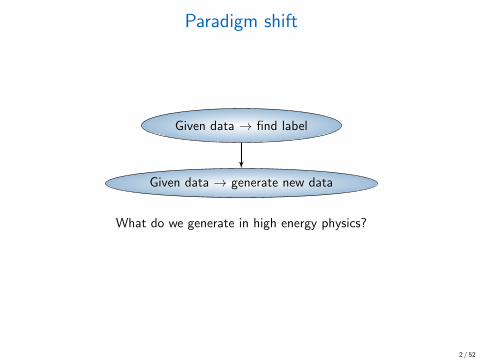
Paradigm shift
Given data → find label
Given data → generate new data
What do we generate in high energy physics?
2 / 52
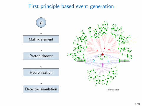
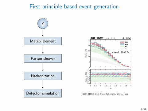
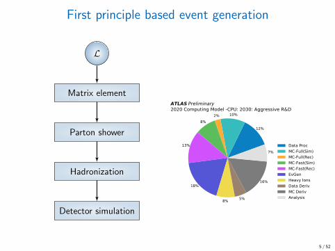
First principle based event generation
L
Matrix element
Parton shower
Hadronization
Detector simulation
�������������������������
�������������������������
������������������������������������������������������������
������������������������������������������������������������
������������������������������������
������������������������������������
������������������������������������
������������������������������������
���������������������������������������������������������
���������������������������������������������������������
������������
������������
������������������
������������������
��������������������
��������������������
������������������
������������������
��������������������
��������������������
������������������
������������������
��������������������
��������������������
��������������������
��������������������
������������������������
������������������������
������������������������
������������������������
��������������������
��������������������
������������������
������������������������
������������
������������������
���������������
���������������
������������������
������������������
�������������������������
�������������������������
���������������
���������������
������������������
������������������
������������������������
������������������
������������������
������������
������������
������������������
������������������
����������
����������
����������
����������
������������������
������������������ ���
������������
���������������
������������������
������������������
���������������
���������������
����������
����������
������������������
������������������
������������
������������
���������������
���������������
��������������������
��������������������
������������
������������
������������������
������������������
������������������������������������
��������������������������������������
����������
������������
���������������
���������������
���������������
���������������
a sherpa artist
3 / 52
First principle based event generation
L
Matrix element
Parton shower
Hadronization
Detector simulation
0.60.70.80.9
11.11.2
0 0.5 1 1.5 2 2.5 3 3.5 4
HN3LO + NNLOJET �s� = 13 TeV
Rati
oto
NNLO
yH
0
5
10
15
20
25HN3LO + NNLOJET �s� = 13 TeV
� [�R;�F] = (¼,½,1) MH
d�H /dy
H[p
b]
p p � H + X
LONLONNLON3LO
HN3LO + NNLOJET �s� = 13 TeV
� [�R;�F] = (¼,½,1) MH
LONLONNLON3LO
0
2
4
6
8
10
12
d�
n/d
Y[T
#]
GPLGPLLGP
L3GP
�4 �3 �2 �1 0 1 2 3 40.8
0.9
1
Y
d�
NN
LO
/dY.
d�
N3L
O/d
Y
pp ! H + X
G>*!Rjh2oJJ>h kyR9 LLGPµF = µR = mh/2
Figure 2: Higgs boson rapidity distribution. Figures from Refs. [19, 20].
�(scale) �(PDF-TH) �(EW) �(t, b, c) �(1/mt) �(PDF) �(↵s)
+0.10 pb�1.15 pb ±0.56 pb ±0.49 pb ±0.40 pb ±0.49 pb ± 0.89 pb +1.25 pb
�1.26 pb
+0.21%�2.37% ±1.16% ±1% ±0.83% ±1% ±1.85% +2.59%
�2.62%
Table 1: Status of the theory uncertainties on Higgs boson production in gluon fusion atp
s = 13 TeV. The table is taken from Ref. [83] and the LHC Higgs WG1 TWiki, with �(trunc)
removed after the work of Ref. [18]. The value for �(EW) was a rough estimate when Ref. [83]
was published. Meanwhile the order of magnitude has been confirmed by the calculations of
Refs. [84–88].
Two-loop electroweak corrections to Higgs production in gluon fusion were
calculated in Refs. [89, 90, 78]. The mixed QCD-EW corrections which ap-
pear at two loops for the first time were calculated directly in Ref. [91], where
however the unphysical limit mZ , mW � mH was employed. In Refs. [84–86],
this restriction was lifted and the mixed QCD-EW corrections at order ↵2↵2s
were calculated, where the real radiation contributions were included in the soft
gluon approximation. It was found that the increase in the total cross section
between pure NLO QCD and NLO QCD+EW is about 5.3%. The calculation
of Ref. [86] has been confirmed by Ref. [87], where also the hard real radiation
was calculated, in the limit of small vector boson masses, corroborating the va-
10
[1807.11501] Cieri, Chen, Gehrmann, Glover, Huss
4 / 52
First principle based event generation
L
Matrix element
Parton shower
Hadronization
Detector simulation
Data Proc
12%
MC-Full(Sim)
10%
MC-Full(Rec)
2%
MC-Fast(Sim)
8%
MC-Fast(Rec)
13%
EvGen
18%
Heavy Ions
8%
Data Deriv
5%
MC Deriv
16%
Analysis
7%
ATLAS Preliminary2020 Computing Model -CPU: 2030: Aggressive R&D
Data ProcMC-Full(Sim)MC-Full(Rec)MC-Fast(Sim)MC-Fast(Rec)EvGenHeavy IonsData DerivMC DerivAnalysis
5 / 52
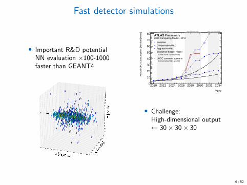
Fast detector simulations
• Important R&D potentialNN evaluation ×100-1000faster than GEANT4
Year
2020 2022 2024 2026 2028 2030 2032 2034
year
s]⋅
Ann
ual C
PU
Con
sum
ptio
n [M
HS
06
0
10
20
30
40
50
60
70
80=55)µRun 3 ( =88-140)µRun 4 ( =165-200)µRun 5 (
2020 Computing Model - CPU
BaselineConservative R&DAggressive R&DSustained budget model(+10% +20% capacity/year)
LHCC common scenario=200)µ(Conservative R&D,
ATLAS Preliminary
• Challenge:High-dimensional output← 30× 30× 30
6 / 52
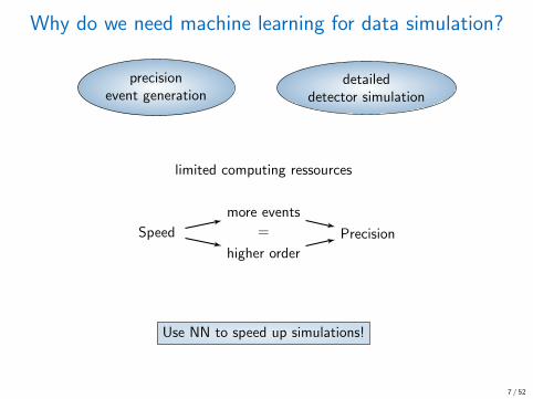
Why do we need machine learning for data simulation?
precisionevent generation
detaileddetector simulation
limited computing ressources
Speed
more events
=
higher order
Precision
Use NN to speed up simulations!
7 / 52
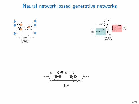
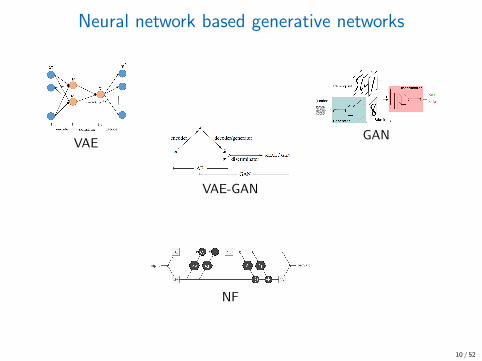
Neural network based generative networks
VAE
all kinds of hybridsVAE-GAN
GAN
NF
8 / 52

Neural network based generative networks
VAE
all kinds of hybrids
VAE-GAN
GAN
NF
9 / 52
Neural network based generative networks
VAE
all kinds of hybrids
VAE-GAN
GAN
NF
10 / 52
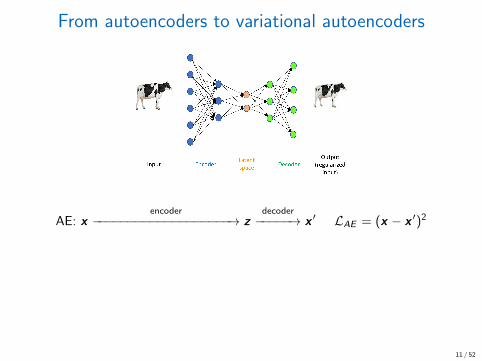
From autoencoders to variational autoencoders
AE: xencoder
−−−−−−−−−−−−−−−−−−−→ zdecoder−−−−−→ x ′ LAE = (x − x ′)2
Loss enforces Gaussian latent space
LVAE = LAE + β · KL(N (µ, σ)|N (0, 1)) ← similarity measure
11 / 52

From autoencoders to variational autoencoders
AE: xencoder
−−−−−−−−−−−−−−−−−−−→ zdecoder−−−−−→ x ′ LAE = (x − x ′)2
VAE: xencoder−−−−−→
(µσ
)sample
−−−−−−−−→z∼N (µ,σ)
zdecoder−−−−−→ x ′ LVAE = LAE + Llat
Loss enforces Gaussian latent space
LVAE = LAE + β · KL(N (µ, σ)|N (0, 1)) ← similarity measure
12 / 52
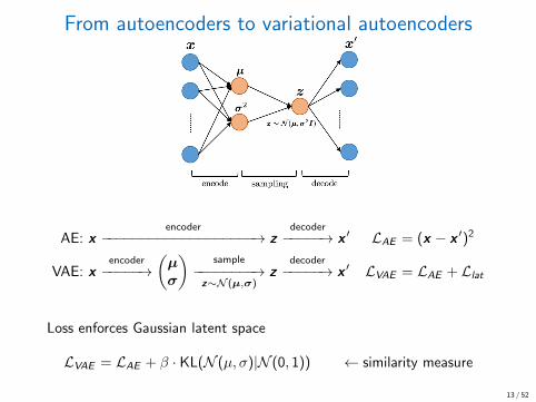
From autoencoders to variational autoencoders
AE: xencoder
−−−−−−−−−−−−−−−−−−−→ zdecoder−−−−−→ x ′ LAE = (x − x ′)2
VAE: xencoder−−−−−→
(µσ
)sample
−−−−−−−−→z∼N (µ,σ)
zdecoder−−−−−→ x ′ LVAE = LAE + Llat
Loss enforces Gaussian latent space
LVAE = LAE + β · KL(N (µ, σ)|N (0, 1)) ← similarity measure
13 / 52

Interlude: KL Divergence
• Distance measure for probability distributions P and Q
• DKL(P ‖ Q) =∫∞−∞ p(x) log
(p(x)q(x)
)dx
By Mundhenk at English Wikipedia, CC BY-SA 3.0
DKL(N (µ, σ) ‖ N (0, 1)) =1
2(1 + log(σ2)− µ2 − σ2)
14 / 52
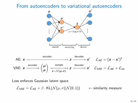
From autoencoders to variational autoencoders
AE: xencoder
−−−−−−−−−−−−−−−−−−−→ zdecoder−−−−−→ x ′ LAE = (x − x ′)2
VAE: xencoder−−−−−→
(µσ
)sample
−−−−−−−−→z∼N (µ,σ)
zdecoder−−−−−→ x ′ LVAE = LAE + Llat
Loss enforces Gaussian latent space
LVAE = LAE + β · KL(N (µ, σ)|N (0, 1)) ← similarity measure
= LAE +β
2
∑
j
1 + log(σ2j )− µ2
j − σ2j
15 / 52

From autoencoders to variational autoencoders
AE: xencoder
−−−−−−−−−−−−−−−−−−−→ zdecoder−−−−−→ x ′ LAE = (x − x ′)2
VAE: xencoder−−−−−→
(µσ
)sample
−−−−−−−−→z∼N (µ,σ)
zdecoder−−−−−→ x ′ LVAE = LAE + Llat
Loss enforces Gaussian latent space
LVAE = LAE + β · KL(N (µ, σ)|N (0, 1)) ← similarity measure
= LAE +β
2
∑
j
1 + log(σ2j )− µ2
j − σ2j
16 / 52
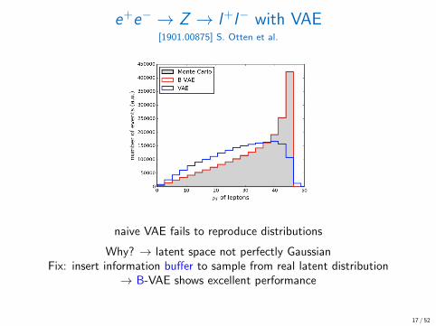
e+e− → Z → l+l− with VAE[1901.00875] S. Otten et al.
naive VAE fails to reproduce distributions
Why? → latent space not perfectly GaussianFix: insert information buffer to sample from real latent distribution
→ B-VAE shows excellent performance
17 / 52

Detector simulation with BIB-AE PPBounded-Information-Bottleneck autoencoder with post processing
18 / 52
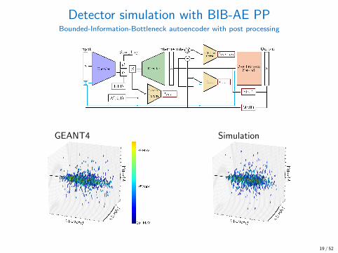
Detector simulation with BIB-AE PPBounded-Information-Bottleneck autoencoder with post processing
GEANT4 Simulation
19 / 52

Generative Adversarial Networks
Discriminator
LD =⟨− logD(x)
⟩x∼PTruth
+⟨− log(1− D(x))
⟩x∼PGen
Generator
LG =⟨− logD(x)
⟩x∼PGen
20 / 52

Training the Discriminator
Discriminator loss
0 = gen 0.2 0.4 0.6 0.8 1 = trueD(x)
0
1
2
3
4
5
LD
true DS generated DS
Minimize LD =⟨− logD(x)
⟩x∼PT
+⟨− log(1− D(x))
⟩x∼PG
21 / 52
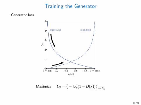
Training the Generator
Generator loss
0 = gen 0.2 0.4 0.6 0.8 1 = trueD(x)
0
1
2
3
4
5
LG
improved standard
Maximize LG =⟨− log(1− D(x))
⟩x∼PG
22 / 52
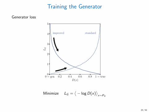
Training the Generator
Generator loss
0 = gen 0.2 0.4 0.6 0.8 1 = trueD(x)
0
1
2
3
4
5
LG
improved standard
Minimize LG =⟨− logD(x)
⟩x∼PG
23 / 52
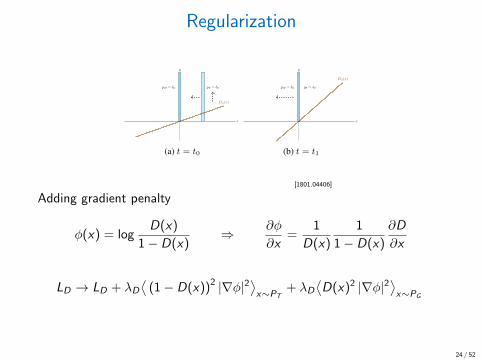
Regularization
Which Training Methods for GANs do actually Converge?
pD = �0 p✓ = �✓
D (x)
x
y
(a) t = t0
pD = �0 p✓ = �✓
D (x)
x
y
(b) t = t1
Figure 1. Visualization of the counterexample showing that gra-dient descent based GAN optimization is not always convergent:(a) In the beginning, the discriminator pushes the generator towardsthe true data distribution and the discriminator’s slope increases.(b) When the generator reaches the target distribution, the slope ofthe discriminator is largest, pushing the generator away from thetarget distribution. This results in oscillatory training dynamicsthat never converge.
than 1, the training algorithm will converge to (✓⇤, ⇤) withlinear rate O(|�max|k) where �max is the eigenvalue ofF 0(✓⇤, ⇤) with the biggest absolute value. If all eigenval-ues of F 0(✓⇤, ⇤) are on the unit circle, the algorithm canbe convergent, divergent or neither, but if it is convergentit will generally converge with a sublinear rate. A similarresult (Khalil, 1996; Nagarajan & Kolter, 2017) also holdsfor the (idealized) continuous system
✓✓(t)
(t)
◆=
✓�r L(✓, )r✓L(✓, )
◆(3)
which corresponds to training the GAN with infinitely smalllearning rate: if all eigenvalues of the Jacobian v0(✓⇤, ⇤)at a stationary point (✓⇤, ⇤) have negative real-part, thecontinuous system converges locally to (✓⇤, ⇤) with lin-ear convergence rate. On the other hand, if v0(✓⇤, ⇤) haseigenvalues with positive real-part, the continuous systemis not locally convergent. If all eigenvalues have zero real-part, it can be convergent, divergent or neither, but if it isconvergent, it will generally converge with a sublinear rate.
For simultaneous gradient descent linear convergence canbe achieved if and only if all eigenvalues of the Jacobianof the gradient vector field v(✓, ) have negative real part(Mescheder et al., 2017). This situation was also consideredby Nagarajan & Kolter (2017) who examined the asymptoticcase of step sizes h that go to 0 and proved local convergencefor absolutely continuous generator and data distributionsunder certain regularity assumptions.
2.2. The Dirac-GAN
Simple experiments, simple theorems are the buildingblocks that help us understand more complicated systems.
Ali Rahimi - Test of Time Award speech, NIPS 2017
In this section, we describe a simple yet prototypical coun-terexample which shows that in the general case unregular-ized GAN training is neither locally nor globally convergent.
Definition 2.1. The Dirac-GAN consists of a (univariate)generator distribution p✓ = �✓ and a linear discriminatorD (x) = · x. The true data distribution pD is given by aDirac-distribution concentrated at 0.
Note that for the Dirac-GAN, both the generator and thediscriminator have exactly one parameter. This situationis visualized in Figure 1. In this setup, the GAN trainingobjective (1) is given by
L(✓, ) = f( ✓) + f(0) (4)
While using linear discriminators might appear restrictive,the class of linear discriminators is in fact as powerful asthe class of all real-valued functions for this example: whenwe use f(t) = � log(1 + exp(�t)) and we take the supre-mum over in (4), we obtain (up to scalar and additiveconstants) the Jensen-Shannon divergence between p✓ andpD. The same holds true for the Wasserstein-divergence,when we use f(t) = t and put a Lipschitz constraint on thediscriminator (see Section 3.1).
We show that the training dynamics of GANs do not con-verge in this simple setup.
Lemma 2.2. The unique equilibrium point of the trainingobjective in (4) is given by ✓ = = 0. Moreover, theJacobian of the gradient vector field at the equilibrium pointhas the two eigenvalues ±f 0(0) i which are both on theimaginary axis.
We now take a closer look at the training dynamics producedby various algorithms for training the Dirac-GAN. First, weconsider the (idealized) continuous system in (3): whileLemma 2.2 shows that the continuous system is generallynot linearly convergent to the equilibrium point, it couldin principle converge with a sublinear convergence rate.However, this is not the case as the next lemma shows:
Lemma 2.3. The integral curves of the gradient vector fieldv(✓, ) do not converge to the Nash-equilibrium. Morespecifically, every integral curve (✓(t), (t)) of the gradientvector field v(✓, ) satisfies ✓(t)2 + (t)2 = const for allt 2 [0,1).
Note that our results do not contradict the results of Nagara-jan & Kolter (2017) and Heusel et al. (2017): our exampleviolates Assumption IV in Nagarajan & Kolter (2017) thatthe support of the generator distribution is equal to the sup-port of the true data distribution near the equilibrium. Italso violates the assumption2 in Heusel et al. (2017) thatthe optimal discriminator parameter vector is a continuousfunction of the current generator parameters. In fact, unless
2This assumption is usually even violated by Wasserstein-GANs, as the optimal discriminator parameter vector as a functionof the current generator parameters can have discontinuities nearthe Nash-equilibrium. See Section 3.1 for details.
[1801.04406]
Adding gradient penalty
φ(x) = logD(x)
1− D(x)⇒ ∂φ
∂x=
1
D(x)
1
1− D(x)
∂D
∂x
LD → LD + λD⟨
(1− D(x))2 |∇φ|2⟩x∼PT
+ λD⟨D(x)2 |∇φ|2
⟩x∼PG
24 / 52

What is the statistical value of GANned events?[2008.06545]
• Camel function
• Sample vs. GAN vs. 5 param.-fit
Evaluation on quantiles:
MSE∗ =
Nquant∑
j=1
(pj −
1
Nquant
)2
25 / 52

What is the statistical value of GANned events?[2008.06545]
• Camel function
• Sample vs. GAN vs. 5 param.-fit
Evaluation on quantiles:
MSE∗ =
Nquant∑
j=1
(pj −
1
Nquant
)2
→ Amplification factor 2.5
Sparser data → bigger amplification
26 / 52
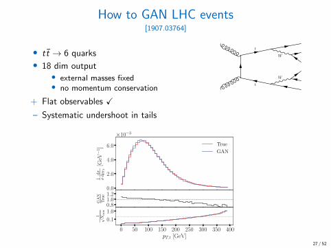
How to GAN LHC events[1907.03764]
• tt → 6 quarks
• 18 dim output• external masses fixed• no momentum conservation
+ Flat observables X
– Systematic undershoot in tails
→ improve network (symmetries, preprocessing, . . . ) X
0.0
2.0
4.0
6.0
1 �d�
dp T
,t[G
eV�
1]
⇥10�3
True
GAN
pT,t [GeV]0.81.01.2
GA
NTru
e
0 50 100 150 200 250 300 350 400pT,t [GeV]
0.1
1.0
1p
Ncu
m
27 / 52
t
t
W
W

How to GAN LHC events[1907.03764]
• tt → 6 quarks
• 18 dim output• external masses fixed• no momentum conservation
+ Flat observables X
– Systematic undershoot in tails→ improve network (symmetries, preprocessing, . . . ) X
unpublished 28 / 52
t
t
W
W

Generating the high-dim. difference of distributions[1912.08824]
• Necessary to include negative events
• Beat bin-induced uncertainty
∆B−S > max(∆B ,∆S)
• Applications:
- Background subtraction, soft-collinear subtraction, ...
G{r}
c ∈ CB−S ∪ CS
{xG , c}
c ∈ CS
DB
DS
{xB}
{xS}
Data B
Data S
LDB
LDS
LG
29 / 52
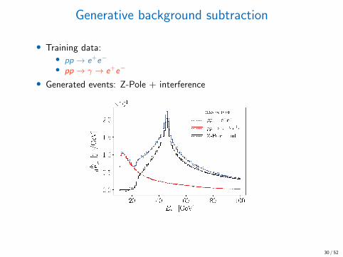
Generative background subtraction
• Training data:• pp → e+e−
• pp → γ → e+e−
• Generated events: Z-Pole + interference
30 / 52
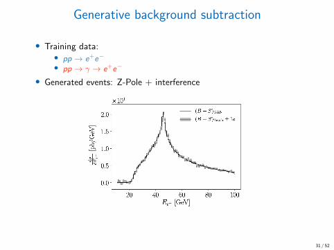
Generative background subtraction
• Training data:• pp → e+e−
• pp → γ → e+e−
• Generated events: Z-Pole + interference
31 / 52

Information in distributions
0.0 0.5 1.0 1.5 2.0 2.5 3.0 3.5 4.0x
0.0
0.5
1.0
1.5
2.0
2.5
3.0
3.5
4.0
y
Information in space distribution(what we want)
=
0.0 0.5 1.0 1.5 2.0 2.5 3.0 3.5 4.0x
0.0
0.5
1.0
1.5
2.0
2.5
3.0
3.5
4.0
y
Information in weight(what we have)
32 / 52

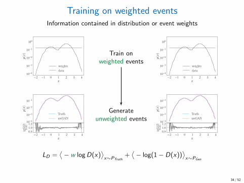
Training on weighted eventsInformation contained in distribution or event weights
−2 −1 0 1 2 3 4x
10−4
10−3
10−2
10−1
100
p(x
)
weights
data
−2 −1 0 1 2 3 4x
10−4
10−3
10−2
10−1
100
p(x
)
weights
data
−2 −1 0 1 2 3 4x
10−4
10−3
10−2
10−1
100
p(x
)
weights
data
combined
Train onweighted events
10−4
10−3
10−2
10−1
p(x
)
Truth
uwGAN
−2 −1 0 1 2 3 4x
0.81.01.2
uwG
AN
Tru
th
Generateunweighted events
LD =⟨− w logD(x)
⟩x∼PTruth
+⟨− log(1− D(x))
⟩x∼PGen
33 / 52
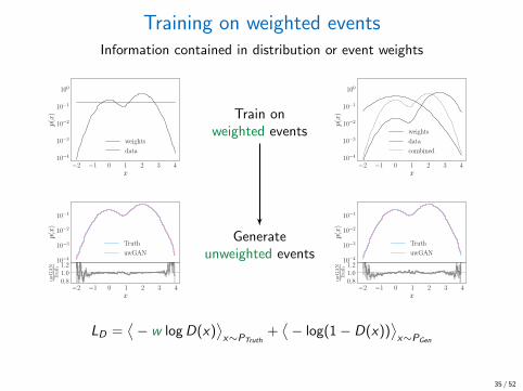
Training on weighted eventsInformation contained in distribution or event weights
−2 −1 0 1 2 3 4x
10−4
10−3
10−2
10−1
100
p(x
)
weights
data
−2 −1 0 1 2 3 4x
10−4
10−3
10−2
10−1
100
p(x
)
weights
data
−2 −1 0 1 2 3 4x
10−4
10−3
10−2
10−1
100
p(x
)
weights
data
combined
Train onweighted events
10−4
10−3
10−2
10−1
p(x
)
Truth
uwGAN
−2 −1 0 1 2 3 4x
0.81.01.2
uwG
AN
Tru
th
10−4
10−3
10−2
10−1
p(x
)
Truth
uwGAN
−2 −1 0 1 2 3 4x
0.81.01.2
uwG
AN
Tru
th
Generateunweighted events
LD =⟨− w logD(x)
⟩x∼PTruth
+⟨− log(1− D(x))
⟩x∼PGen
34 / 52
Training on weighted eventsInformation contained in distribution or event weights
−2 −1 0 1 2 3 4x
10−4
10−3
10−2
10−1
100
p(x
)
weights
data
−2 −1 0 1 2 3 4x
10−4
10−3
10−2
10−1
100
p(x
)
weights
data
−2 −1 0 1 2 3 4x
10−4
10−3
10−2
10−1
100
p(x
)
weights
data
combined
Train onweighted events
10−4
10−3
10−2
10−1
p(x
)
Truth
uwGAN
−2 −1 0 1 2 3 4x
0.81.01.2
uwG
AN
Tru
th
10−4
10−3
10−2
10−1
p(x
)
Truth
uwGAN
−2 −1 0 1 2 3 4x
0.81.01.2
uwG
AN
Tru
th
Generateunweighted events
LD =⟨− w logD(x)
⟩x∼PTruth
+⟨− log(1− D(x))
⟩x∼PGen
35 / 52
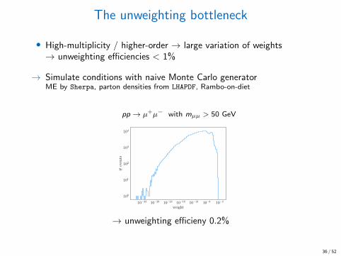
The unweighting bottleneck
• High-multiplicity / higher-order → large variation of weights→ unweighting efficiencies < 1%
→ Simulate conditions with naive Monte Carlo generatorME by Sherpa, parton densities from LHAPDF, Rambo-on-diet
pp → µ+µ− with mµµ > 50 GeV
10−33 10−28 10−23 10−18 10−13 10−8 10−3
weight
100
101
102
103
104
#ev
ents
→ unweighting efficieny 0.2%
36 / 52
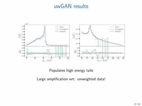
uwGAN results
0.0
0.2
0.4
0.6
0.8
1.0
1.2
1.4
1 σdσ
dpT,µ−
×10−1
Train
Unweighted
uwGAN
0 20 40 60 80 100
pT,µ− [GeV]
0.5
1.0
1.5
2.0
XT
ruth
10−4
10−3
10−2
10−1
1 σdσ
dmµ−µ
+
Train
Unweighted
uwGAN
50 75 100 125 150 175 200 225 250
mµ−µ+ [GeV]
0.5
1.0
1.5
2.0
XT
ruth
Populates high energy tails
Large amplification wrt. unweighted data!
37 / 52
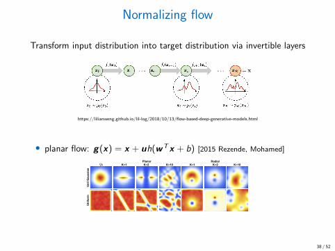
Normalizing flow
Transform input distribution into target distribution via invertible layers
https://lilianweng.github.io/lil-log/2018/10/13/flow-based-deep-generative-models.html
• planar flow: g(x) = x + uh(wTx + b) [2015 Rezende, Mohamed]Variational Inference with Normalizing Flows
and involve matrix inverses that can be numerically unsta-ble. We therefore require normalizing flows that allow forlow-cost computation of the determinant, or where the Ja-cobian is not needed at all.
4.1. Invertible Linear-time Transformations
We consider a family of transformations of the form:
f(z) = z + uh(w>z + b), (10)
where � = {w 2 IRD,u 2 IRD, b 2 IR} are free pa-rameters and h(·) is a smooth element-wise non-linearity,with derivative h0(·). For this mapping we can computethe logdet-Jacobian term in O(D) time (using the matrixdeterminant lemma):
(z) = h0(w>z + b)w (11)���det @f@z
��� = | det(I + u (z)>)| = |1 + u> (z)|. (12)
From (7) we conclude that the density qK(z) obtained bytransforming an arbitrary initial density q0(z) through thesequence of maps fk of the form (10) is implicitly givenby:
zK = fK � fK�1 � . . . � f1(z)
ln qK(zK) = ln q0(z)�KX
k=1
ln |1 + u>k k(zk�1)|. (13)
The flow defined by the transformation (13) modifies theinitial density q0 by applying a series of contractions andexpansions in the direction perpendicular to the hyperplanew>z+b = 0, hence we refer to these maps as planar flows.
As an alternative, we can consider a family of transforma-tions that modify an initial density q0 around a referencepoint z0. The transformation family is:
f(z) = z + �h(↵, r)(z� z0), (14)����det@f
@z
���� = [1 + �h(↵, r)]d�1
[1 + �h(↵, r) + �h0(↵, r)r)] ,
where r = |z � z0|, h(↵, r) = 1/(↵ + r), and the param-eters of the map are � = {z0 2 IRD,↵ 2 IR+,� 2 IR}.This family also allows for linear-time computation of thedeterminant. It applies radial contractions and expansionsaround the reference point and are thus referred to as radialflows. We show the effect of expansions and contractionson a uniform and Gaussian initial density using the flows(10) and (14) in figure 1. This visualization shows that wecan transform a spherical Gaussian distribution into a bi-modal distribution by applying two successive transforma-tions.
Not all functions of the form (10) or (14) will be invert-ible. We discuss the conditions for invertibility and how tosatisfy them in a numerically stable way in the appendix.
K=1 K=2Planar Radial
q0 K=1 K=2K=10 K=10
Uni
t Gau
ssia
nU
nifo
rm
Figure 1. Effect of normalizing flow on two distributions.
Inference network Generative model
Figure 2. Inference and generative models. Left: Inference net-work maps the observations to the parameters of the flow; Right:generative model which receives the posterior samples from theinference network during training time. Round containers repre-sent layers of stochastic variables whereas square containers rep-resent deterministic layers.
4.2. Flow-Based Free Energy Bound
If we parameterize the approximate posterior distributionwith a flow of length K, q�(z|x) := qK(zK), the free en-ergy (3) can be written as an expectation over the initialdistribution q0(z):
F(x) = Eq�(z|x)[log q�(z|x)� log p(x, z)]
= Eq0(z0) [ln qK(zK)� log p(x, zK)]
= Eq0(z0) [ln q0(z0)]� Eq0(z0) [log p(x, zK)]
� Eq0(z0)
"KX
k=1
ln |1 + u>k k(zk�1)|#
. (15)
Normalizing flows and this free energy bound can be usedwith any variational optimization scheme, including gener-alized variational EM. For amortized variational inference,we construct an inference model using a deep neural net-work to build a mapping from the observations x to theparameters of the initial density q0 = N (µ,�) (µ 2 IRD
and � 2 IRD) as well as the parameters of the flow �.
4.3. Algorithm Summary and Complexity
The resulting algorithm is a simple modification of theamortized inference algorithm for DLGMs described by(Kingma & Welling, 2014; Rezende et al., 2014), whichwe summarize in algorithm 1. By using an inference net-
38 / 52
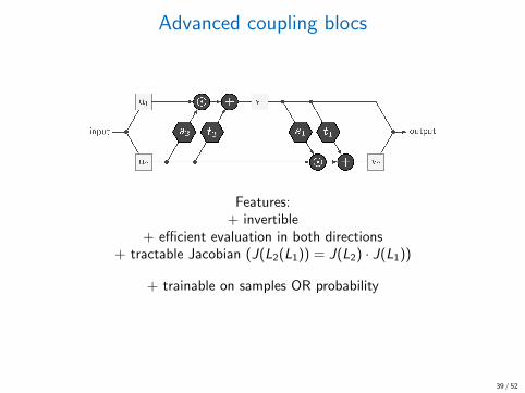
Advanced coupling blocs
Features:+ invertible
+ efficient evaluation in both directions+ tractable Jacobian (J(L2(L1)) = J(L2) · J(L1))
+ trainable on samples OR probability
39 / 52
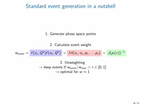
Standard event generation in a nutshell
1. Generate phase space points
2. Calculate event weight
wevent = f (x1,Q2)f (x2,Q
2) × M(x1, x2, p1, . . . pn) × J(pi (r))−1
3. Unweighting→ keep events if wevent/wmax > r ∈ [0, 1]
→ optimal for w ≈ 1
40 / 52
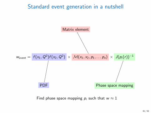
Standard event generation in a nutshell
Matrix element
wevent = f (x1,Q2)f (x2,Q
2) × M(x1, x2, p1, . . . pn) × J(pi (r))−1
PDF Phase space mapping
Find phase space mapping pi such that w ≈ 1
41 / 52
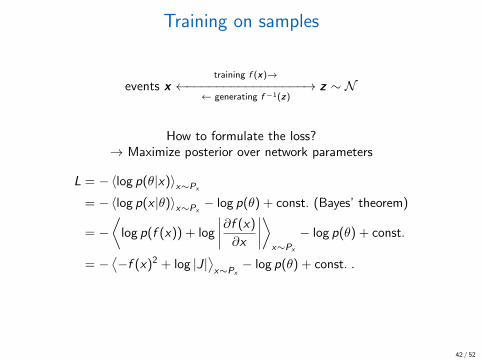
Training on samples
events xtraining f (x)→
←−−−−−−−−−−−−−−−−→← generating f −1(z)
z ∼ N
How to formulate the loss?→ Maximize posterior over network parameters
L = −〈log p(θ|x)〉x∼Px
= −〈log p(x |θ)〉x∼Px− log p(θ) + const. (Bayes’ theorem)
= −⟨
log p(f (x)) + log
∣∣∣∣∂f (x)
∂x
∣∣∣∣⟩
x∼Px
− log p(θ) + const.
= −⟨−f (x)2 + log |J|
⟩x∼Px
− log p(θ) + const. .
42 / 52
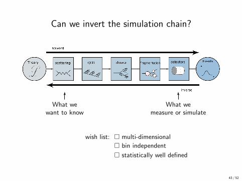
Can we invert the simulation chain?
What wewant to know
What wemeasure or simulate
wish list: � multi-dimensional
� bin independent
� statistically well defined
43 / 52

Invertible networks
(xpart
) Pythia,Delphes:g→←−−−−−−−−−−−−−−−−→
← unfolding:g
(xdet)
[1808.04730] L. Ardizzone, J. Kruse, S. Wirkert, D. Rahner,
E. W. Pellegrini, R. S. Klessen, L. Maier-Hein, C. Rother, U. Kothe
+ Bijective mapping
+ Tractable Jacobian
+ Fast evaluation in both directions
+ Arbitrary networks s and t
44 / 52

Inverting detector effects
0.0
1.0
2.0
3.0
4.0
5.0
6.0
1 σdσ
dpT,q
2[G
eV−
1]
×10−2
2 jet no ISR
Parton Truth
Parton INN
Detector Truth
Detector INN
0 20 40 60 80 100 120pT,q2
[GeV]
0.81.01.2
INN
Tru
th
0.0
0.5
1.0
1.5
2.0
2.5
3.0
1 σdσ
dMW,reco
[GeV−
1]
×10−1
2 jet no ISR
Parton Truth
Parton INN
Detector Truth
Detector INN
70 75 80 85 90 95MW,reco [GeV]
0.81.01.2
INN
Tru
th
multi-dimensional X bin independent X statistically well defined ?
45 / 52
• pp → ZW → (ll)(jj)
• Train: parton → detector
• Evaluate: parton ← detectorW
Z
j
j
ℓ+
ℓ−
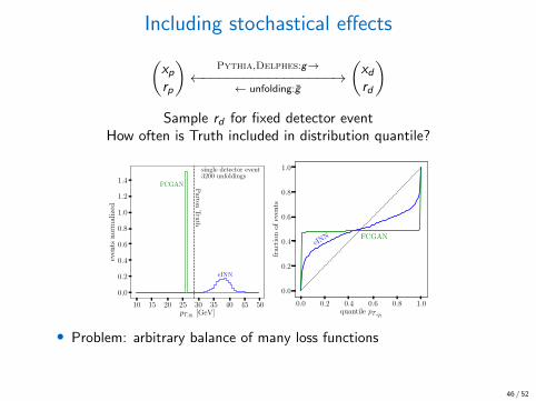
Including stochastical effects
(xprp
)Pythia,Delphes:g→
←−−−−−−−−−−−−−−−−→← unfolding:g
(xdrd
)
Sample rd for fixed detector eventHow often is Truth included in distribution quantile?
10 15 20 25 30 35 40 45 50pT,q1
[GeV]
0.0
0.2
0.4
0.6
0.8
1.0
1.2
1.4
even
tsn
orm
aliz
ed
eINN
FCGAN
single detector event3200 unfoldings
Parton
Tru
th
0.0 0.2 0.4 0.6 0.8 1.0quantile pT,q1
0.0
0.2
0.4
0.6
0.8
1.0
frac
tion
ofev
ents
eINN FCGAN
• Problem: arbitrary balance of many loss functions
46 / 52
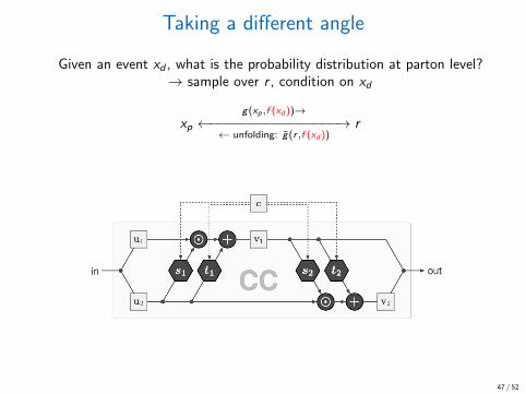
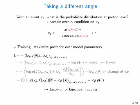
Taking a different angle
Given an event xd , what is the probability distribution at parton level?→ sample over r , condition on xd
xpg(xp,f (xd ))→
←−−−−−−−−−−−−−−−−→← unfolding: g(r ,f (xd ))
r
→ Training: Maximize posterior over model parameters
L = −〈log p(θ|xp, xd)〉xp∼Pp,xd∼Pd
= −〈log p(xp|θ, xd)〉xp∼Pp,xd∼Pd− log p(θ) + const. ← Bayes
= −⟨
log p(g(xp, xd)) + log
∣∣∣∣∂g(xp, xd)
∂xp
∣∣∣∣⟩− log p(θ)← change of var
=⟨0.5||g(xp, f (xd))||22 − log |J|
⟩xp∼Pp,xd∼Pd
− log p(θ)
→ Jacobian of bijective mapping
47 / 52
Taking a different angle
Given an event xd , what is the probability distribution at parton level?→ sample over r , condition on xd
xpg(xp,f (xd ))→
←−−−−−−−−−−−−−−−−→← unfolding: g(r ,f (xd ))
r
→ Training: Maximize posterior over model parameters
L = −〈log p(θ|xp, xd)〉xp∼Pp,xd∼Pd
= −〈log p(xp|θ, xd)〉xp∼Pp,xd∼Pd− log p(θ) + const. ← Bayes
= −⟨
log p(g(xp, xd)) + log
∣∣∣∣∂g(xp, xd)
∂xp
∣∣∣∣⟩− log p(θ)← change of var
=⟨0.5||g(xp, f (xd))||22 − log |J|
⟩xp∼Pp,xd∼Pd
− log p(θ)
→ Jacobian of bijective mapping
48 / 52
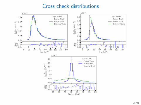
Cross check distributions
0.0
0.5
1.0
1.5
2.0
2.5
1 σdσ
dpT,q
1[G
eV−
1]
×10−2
2 jet no ISR
Parton Truth
Parton cINN
Detector Truth
0 25 50 75 100 125 150 175 200pT,q1
[GeV]
0.81.01.2
cIN
NT
ruth
0.0
1.0
2.0
3.0
4.0
5.0
6.0
1 σdσ
dpT,q
2[G
eV−
1]
×10−2
2 jet no ISR
Parton Truth
Parton cINN
Detector Truth
0 20 40 60 80 100 120 140pT,q2
[GeV]
0.81.01.2
cIN
NT
ruth
0.0
0.5
1.0
1.5
2.0
2.5
3.0
1 σdσ
dMW,reco
[GeV−
1]
×10−1
2 jet no ISR
Parton Truth
Parton cINN
Detector Truth
65 70 75 80 85 90 95 100MW,reco [GeV]
0.81.01.2
cIN
NT
ruth
49 / 52
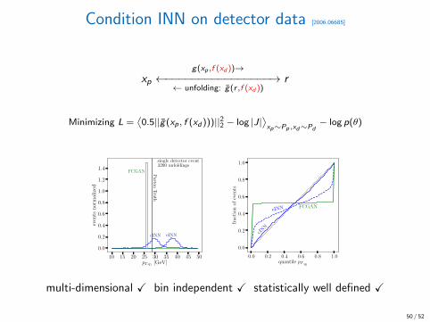
Condition INN on detector data [2006.06685]
xpg(xp,f (xd ))→
←−−−−−−−−−−−−−−−−→← unfolding: g(r ,f (xd ))
r
Minimizing L =⟨0.5||g(xp , f (xd )))||22 − log |J|
⟩xp∼Pp ,xd∼Pd
− log p(θ)
10 15 20 25 30 35 40 45 50pT,q1
[GeV]
0.0
0.2
0.4
0.6
0.8
1.0
1.2
1.4
even
tsn
orm
aliz
ed
cINN eINN
FCGAN
single detector event3200 unfoldings
Parton
Tru
th
0.0 0.2 0.4 0.6 0.8 1.0quantile pT,q1
0.0
0.2
0.4
0.6
0.8
1.0
frac
tion
ofev
ents
cINN
eINN FCGAN
multi-dimensional X bin independent X statistically well defined X
50 / 52

Summary
• Three types of generative models VAE, GAN, NF
• VAE: latent space encoding, KL loss can limit performance
• GAN: based on simple classifier, efficient training if stabilized
• NF: invertible, useable to train directly on probability
51 / 52

Now it’s your turn
52 / 52