generic programming with adjunctions · generic programming with adjunctions 3 haskell...
TRANSCRIPT

Generic Programming with Adjunctions
Ralf Hinze
Department of Computer Science, University of OxfordWolfson Building, Parks Road, Oxford, OX1 3QD, England
http://www.cs.ox.ac.uk/ralf.hinze/
Abstract. Adjunctions are among the most important constructionsin mathematics. These lecture notes show they are also highly relevantto datatype-generic programming. First, every fundamental datatype—sums, products, function types, recursive types—arises out of an adjunc-tion. The defining properties of an adjunction give rise to well-known lawsof the algebra of programming. Second, adjunctions are instrumental inunifying and generalising recursion schemes. We discuss a multitude ofbasic adjunctions and show that they are directly relevant to program-ming and to reasoning about programs.
1 Introduction
Haskell programmers have embraced functors [1], natural transformations [2],monads [3], monoidal functors [4] and, perhaps to a lesser extent, initial alge-bras [5] and final coalgebras [6]. It is time for them to turn their attention toadjunctions.
The notion of an adjunction was introduced by Daniel Kan in 1958 [7]. Verybriefly, the functors L and R are adjoint if arrows of type LA→ B are in one-to-one correspondence to arrows of type A→ RB and if the bijection is furthermorenatural in A and B . Adjunctions have proved to be one of the most importantideas in category theory, predominantly due to their ubiquity. Many mathemat-ical constructions turn out to be adjoint functors that form adjunctions, withMac Lane [8, p.vii] famously saying, “Adjoint functors arise everywhere.”
The purpose of these lecture notes is to show that the notion of an adjunc-tion is also highly relevant to programming, in particular, to datatype-genericprogramming. The concept is relevant in at least two different, but related ways.
First, every fundamental datatype—sums, products, function types, recursivetypes—arises out of an adjunction. The categorical ingredients of an adjunctioncorrespond to introduction and elimination rules; the defining properties of anadjunction correspond to β-rules, η-rules and fusion laws, which codify basicoptimisation principles.
Second, adjunctions are instrumental in unifying and generalising recursionschemes. Historically, the algebra of programming [9] is based on the theoryof initial algebras: programs are expressed as folds, and program calculation isbased on the universal property of folds. In a nutshell, the universal property

2 Ralf Hinze
formalises that a fold is the unique solution of its defining equation. It impliescomputation laws and optimisation laws such as fusion. The economy of rea-soning is further enhanced by the principle of duality: initial algebras dualise tofinal coalgebras, and correspondingly folds dualise to unfolds. Two theories forthe price of one.
However, all that glitters is not gold. Most, if not all, programs require sometweaking to be given the form of a fold or an unfold and thus make themamenable to formal manipulation. Somewhat ironically, this is in particular trueof the “Hello, world!” programs of functional programming: factorial, the Fi-bonacci function and append. For instance, append does not have the form of afold as it takes a second argument that is later used in the base case.
In response to this shortcoming a plethora of different recursion schemes hasbeen introduced over the past two decades. Using the concept of an adjunctionmany of these schemes can be unified and generalised. The resulting schemeis called an adjoint fold. A standard fold insists on the idea that the controlstructure of a function ever follows the structure of its input data. Adjoint foldsloosen this tight coupling—the control structure is given implicitly through theadjunction.
Technically, the central idea is to gain flexibility by allowing the argumentof a fold or the result of an unfold to be wrapped up in a functor application.In the case of append, the functor is essentially pairing. Not every functor isadmissible: to preserve the salient properties of folds and unfolds, we require thefunctor to have a right adjoint and, dually, a left adjoint for unfolds. Like folds,adjoint folds are then the unique solutions of their defining equations and, as isto be expected, this dualises to unfolds.
These lecture notes are organised into two major parts. The first part (Sec-tion 2) investigates the use of adjunctions for defining ‘data structures’. It ispartly based on the “Category Theory Primer” distributed at the Spring School[10]. This section includes some background material on category theory, with theaim of making the lecture notes accessible to readers without specialist knowl-edge.
The second part (Section 3) illustrates the use of adjunctions for giving aprecise semantics to ‘algorithms’. It is largely based on the forthcoming arti-cle “Adjoint Folds and Unfolds—An Extended Study” [11]. Some material hasbeen omitted, some new material has been added (Sections 3.3.3 and 3.4.2);furthermore, all of the examples have been reworked.
The two parts can be read fairly independently. Indeed, on a first reading Irecommend to skip to the second part even though it relies on the results of thefirst one. The development in Section 3 is accompanied by a series of examplesin Haskell, which may help in motivating and comprehending the different con-structions. The first part then hopefully helps in gaining a deeper understandingof the material.
The notes are complemented by a series of exercises, which can be used tocheck progress. Some of the exercises form independent threads that introducemore advanced material. As an example, adjunctions are closely related to the

Generic Programming with Adjunctions 3
Haskell programmer’s favourite toy, monads: every adjunction induces a monadand a comonad; conversely, every (co)monad can be defined by an adjunction.These advanced exercises are marked with a ‘∗’.
Enjoy reading!
2 Adjunctions for Data Structures
The first part of these lecture notes is structured as follows. Section 2.1 and 2.2provide some background to category theory, preparing the ground for the re-mainder of these lecture notes. Sections 2.3 and 2.4 show how to model non-recursive datatypes, finite products and sums, categorically. We emphasise thecalculational properties of the constructions, working carefully towards the cen-tral concept of an adjunction, which is then introduced in Section 2.5. This sec-tion discusses fundamental properties of adjunctions and illustrates the conceptwith further examples. In particular, it introduces exponentials, which modelhigher-order function types. Section 2.6 then shows how to capture recursivedatatypes, introducing initial algebras and final coalgebras. Both constructionsarise out of an adjunction, related to free algebras and cofree coalgebras, whichare perhaps less well-known and which are studied in considerable depth. Finally,Section 2.7 introduces an important categorical tool, the Yoneda Lemma, usedrepeatedly in the second part of the lecture notes.
2.1 Category, Functor and Natural Transformation
This section introduces the categorical trinity: category, functor and naturaltransformation. If you are already familiar with the topic, then you can skip thesection and the next, except perhaps for notation. If this is unexplored territory,try to absorb the definitions, study the examples and, most importantly, takeyour time to let the material sink in.
2.1.1 Category. A category consists of objects and arrows between objects.We let C , D etc range over categories. We write A ∶ C to express that A isan object of C . We let A, B etc range over objects. For every pair of objectsA,B ∶ C there is a class of arrows from A to B , denoted C (A,B). If C is obviousfrom the context, we abbreviate f ∶ C (A,B) by f ∶ A → B or by f ∶ B ← A. Wewill also loosely speak of A → B as the type of f . We let f , g etc range overarrows.
For every object A ∶ C there is an arrow idA ∶ A → A, called the identity.Two arrows can be composed if their types match: If f ∶ A → B and g ∶ B → C ,then g ⋅ f ∶ A→ C . We require composition to be associative with identity as itsneutral element.
A category is often identified with its class of objects. For instance, we saythat Set is the category of sets. However, equally, if not more, important are thearrows of a category. So, Set is really the category of sets and total functions.(There is also Rel, the category of sets and relations.) For Set, the identity

4 Ralf Hinze
arrow is the identity function and composition is functional composition. If theobjects have additional structure (monoids, groups etc), then the arrows aretypically structure-preserving maps.
Exercise 1. Define the category Mon, whose objects are monoids and whosearrows are monoid homomorphisms. ⊓⊔
However, the objects of a category are not necessarily sets and the arrowsare not necessarily functions:
Exercise 2. A preorder ≾ is an extreme example of a category: C (A,B) is in-habited if and only if A ≾ B. So each C (A,B) has at most one element. Spellout the details. ⊓⊔
Exercise 3. A monoid is another extreme example of a category: there is exactlyone object. Spell out the details. ⊓⊔
A subcategory S of a category C is a collection of some of the objects andsome of the arrows of C , such that identity and composition are preserved toensure S constitutes a category. In a full subcategory, S (A,B) = C (A,B), forall objects A,B ∶ S .
An arrow f ∶ A→ B is invertible if there is an arrow g ∶ A← B with g ⋅ f = idA
and f ⋅ g = idB . If the inverse arrow exists, it is unique and is written as f ○. Twoobjects A and B are isomorphic, A ≅ B , if there is an invertible arrow f ∶ A→ B .We also write f ∶ A ≅ B ∶ f ○ to express that the arrows f ∶ A→ B and f ○ ∶ A← Bwitness the isomorphism A ≅ B .
Exercise 4. Show that the inverse of an arrow is unique. ⊓⊔
2.1.2 Functor. Every mathematical structure comes equipped with structure-preserving maps; so do categories, where these maps are called functors. (Indeed,category theory can be seen as the study of structure-preserving maps. Mac Lane[8, p.30] writes: “Category theory asks of every type of Mathematical object:‘What are the morphisms?’”) Since a category consists of two parts, objects andarrows, a functor F ∶ C → D consists of a mapping on objects and a mappingon arrows. It is common practice to denote both mappings by the same symbol.We will also loosely speak of F’s arrow part as a ‘map’. The action on arrowshas to respect the types: if f ∶ C (A,B), then F f ∶ D(FA,FB). Furthermore, Fhas to preserve identity and composition:
F idA = idFA , (1)
F (g ⋅ f ) = F g ⋅ F f . (2)
The force of functoriality lies in the action on arrows and in the preservation ofcomposition. We let F, G etc range over functors. A functor F ∶ C → C over acategory C is called an endofunctor.

Generic Programming with Adjunctions 5
Exercise 5. Show that functors preserve isomorphisms.
F f ∶ FA ≅ FB ∶ F f ○ ⇐Ô f ∶ A ≅ B ∶ f ○⊓⊔
∗ Exercise 6. The category Mon has more structure than Set. Define a functorU ∶ Mon → Set that forgets about the additional structure. (The functor U iscalled the forgetful or underlying functor.) ⊓⊔
There is an identity functor, IdC ∶ C → C , and functors can be composed:(G○F)A = G (FA) and (G○F) f = G (F f ). This data turns small categories1 andfunctors into a category, called Cat.
Exercise 7. Show that IdC and G○F are indeed functors. ⊓⊔
2.1.3 Natural Transformation. Let F,G ∶ C → D be two parallel functors.A transformation α ∶ F → G is a collection of arrows, so that for each objectA ∶ C there is an arrow αA ∶ D(FA,GA). In other words, a transformation is amapping from objects to arrows. A transformation is natural, α ∶ F →G, if
Gh ⋅ αA = αA ⋅ Fh , (3)
for all objects A and A and for all arrows h ∶ C (A, A). Note that α is used attwo different instances: D(F A,G A) and D(F A,G A)—we will adopt the habitof decorating instances with a circumflex ( ) and with an inverted circumflex ( ).Now, given α and h, there are essentially two ways of turning F A things into G Athings. The coherence condition (3) demands that they are equal. The conditionis visualised below using a commuting diagram: all paths from the same sourceto the same target lead to the same result by composition.
F AFh
≻ F A
G A
α A⋎
Gh≻ G A
α A⋎
We write α ∶ F ≅ G, if α is a natural isomorphism. As an example, the identityis a natural isomorphism of type F ≅ F. We let α, β etc range over naturaltransformations.
2.2 Opposite, Product and Functor Category
In the previous section we have encountered a few examples of categories. Next,we show how to create new categories from old.
1 To avoid paradoxes, we have to require that the objects of Cat are small, where acategory is called small if the class of objects and the class of all arrows are sets. Bythat token, Set and Cat are not themselves small.

6 Ralf Hinze
2.2.1 Opposite Category. Let C be a category. The opposite category C op
has the same objects as C ; the arrows of C op are in one-to-one correspondenceto the arrows in C , that is, f op ∶ C op(A,B) if and only if f ∶ C (B ,A). Identityand composition are defined flip-wise:
id = idop and f op ⋅ gop = (g ⋅ f )op .
A functor of type C op → D or C → Dop is sometimes called a contravariantfunctor from C to D , the usual kind being styled covariant. The operation (−)opitself can be extended to a covariant functor (−)op ∶ Cat → Cat, whose arrowpart is defined Fop A = FA and Fop f op = (F f )op. We agree that (f op)op = f sothat the operation is an involution. (In later sections, we will often be sloppyand omit the bijection (−)op on arrows.)
A somewhat incestuous example of a contravariant functor is pre-compositionC (−,B) ∶ C op → Set, whose action on arrows is given by C (hop,B) f = f ⋅ h.(Partial applications of mappings and operators are written using ‘categoricaldummies’, where − marks the first and = the second argument if any.) The functorC (−,B) maps an object A to the set of arrows C (A,B) from A to a fixed B ,and it takes an arrow hop ∶ C op(A, A) to a function C (hop,B) ∶ C (A,B) →C (A,B). Dually, post-composition C (A,−) ∶ C → Set is a covariant functordefined C (A, k) f = k ⋅ f .
Exercise 8. Show that C (A,−) and C (−,B) are functors. ⊓⊔
2.2.2 Product Category. Let C1 and C2 be categories. An object of theproduct category C1 × C2 is a pair ⟨A1, A2⟩ of objects A1 ∶ C1 and A2 ∶ C2; anarrow of (C1 ×C2)(⟨A1, A2⟩, ⟨B1, B2⟩) is a pair ⟨f1, f2⟩ of arrows f1 ∶ C1(A1,B1)and f2 ∶ C2(A2,B2). Identity and composition are defined component-wise:
id = ⟨id , id⟩ and ⟨g1, g2⟩ ⋅ ⟨f1, f2⟩ = ⟨g1 ⋅ f1, g2 ⋅ f2⟩ .
The projection functors Outl ∶ C1 × C2 → C1 and Outr ∶ C1 × C2 → C2 are givenby Outl ⟨A1, A2⟩ = A1, Outl ⟨f1, f2⟩ = f1 and Outr ⟨A1, A2⟩ = A2, Outr ⟨f1, f2⟩ = f2.Product categories avoid the need for functors of several arguments. Functorssuch as Outl and Outr from a product category are sometimes called bifunctors.The diagonal functor ∆ ∶ C → C × C is an example of a functor into a productcategory: it duplicates its argument ∆A = ⟨A,A⟩ and ∆f = ⟨f , f ⟩.
If we fix one argument of a bifunctor, we obtain a functor. The converse isnot true: functoriality in each argument separately does not imply functorialityin both. Rather, we have the following: (−⊗ =) ∶ C ×D → E is a bifunctor if andonly if the partial application (A ⊗ −) ∶ D → E is a functor for all A ∶ C , thepartial application (−⊗B) ∶ C → E is a functor for all B ∶ D , and if furthermorethe two collections of unary functors satisfy the exchange law
(A⊗ g) ⋅ (f ⊗ B) = (f ⊗ B) ⋅ (A⊗ g) , (4)

Generic Programming with Adjunctions 7
for all objects A, A, B and B and for all arrows f ∶ C (A, A) and g ∶ D(B, B).Given f and g there are two ways of turning A⊗ B things into A⊗ B things:
A⊗ BA⊗ g
≻ A⊗ B
A⊗ B
f ⊗ B⋎
A⊗ g≻ A⊗ B .
f ⊗ B⋎
f ⊗ g
≻
The coherence condition (4) demands that they are equal. The arrow part of thebifunctor, the diagonal, is then given by either side of (4). The exchange lawcan also be read as two naturality conditions, stating that f ⊗ − and − ⊗ g arenatural transformations!
Exercise 9. Prove the characterisation of bifunctors. ⊓⊔
The corresponding notion of a ‘binatural’ transformation is more straightfor-ward. Let F,G ∶ C ×D → E be two parallel functors. The transformation α ∶ F→Gis natural in both arguments if and only if it is natural in each argument sepa-rately.
Exercise 10. Spell out the details and prove the claim. ⊓⊔
We have noted that pre-composition C (A,−) and post-composition C (−,B)are functors. Pre-composition commutes with post-composition:
C (A, g) ⋅C (f op, B) = C (f op, B) ⋅C (A, g) , (5)
for all f op ∶ C op(A, A) and g ∶ C (B, B). This is an instance of the exchangelaw (4), so it follows that the so-called hom-functor C (−,=) ∶ C op × C → Set isa bifunctor. It maps a pair of objects to the set of arrows between them, theso-called hom-set; its action on arrows is given by
C (f op, g)h = g ⋅ h ⋅ f . (6)
2.2.3 Functor Category. There is an identity natural transformation idF ∶F→F defined idF A = idFA. Natural transformations can be composed: if α ∶ F→Gand β ∶ G → H, then β ⋅ α ∶ F → H is defined (β ⋅ α)A = βA ⋅ αA. Thus, functorsof type C → D and natural transformations between them form a category, thefunctor category DC . (Functor categories are exponentials in Cat, hence thenotation. The next paragraph makes a first step towards proving this fact.)
The application of a functor to an object is itself functorial. Specifically,it is a bifunctor of type (−=) ∶ DC × C → D . Using the characterisation ofbifunctors, we have to show that (F−) ∶ C → D is a functor for each F ∶ DC ,that (−A) ∶ DC → D is a functor for each A ∶ C , and that the two collectionssatisfy the exchange law (4). The former is immediate since (F−) is just F. Thearrow part of the latter is (−A)α = αA. That this action preserves identity

8 Ralf Hinze
and composition is a consequence of the definition of DC . Finally, the coherencecondition for bifunctors (4) is just the naturality condition (3). (Indeed, onecould argue the other way round: the desire to turn functor application into ahigher-order functor determines the concept of a natural transformation and inturn the definition of DC .) For reference, we record that functor application isa bifunctor, whose action on arrows is defined
α f = F f ⋅ αA = αA ⋅ F f . (7)
Let F ∶ C → D be a functor. Pre-composition −○F is itself a functor, onebetween functor categories −○F ∶ E D → E C . The action on arrows, that is,natural transformations, is defined (α○F)A = α (FA). Dually, post-compositionF○− is a functor of type F○− ∶ C E → DE defined (F○α)A = F (αA).
Exercise 11. Show that α○F and F○α are natural transformations. Prove that−○F and F○− preserve identity and composition. ⊓⊔
Pre-composition commutes with post-composition:
(F○β) ⋅ (α○G) = (α○G) ⋅ (F○β) ,
for all α ∶ F → F and β ∶ G → G. Again, it follows that functor composition(−○=) ∶ E D ×DC → E C is a bifunctor.
2.3 Product and Coproduct
Definitions in category theory often take the form of universal constructions, aconcept we explore in this section. The paradigmatic example of this approachis the definition of products—in fact, this is also historically the first example.
2.3.1 Product. A product of two objects B1 and B2 consists of an objectwritten B1×B2 and a pair of arrows outl ∶ B1×B2 → B1 and outr ∶ B1×B2 → B2.These three things have to satisfy the following universal property : for eachobject A and for each pair of arrows f1 ∶ A → B1 and f2 ∶ A → B2, there exists aunique arrow g ∶ A→ B1 ×B2 such that f1 = outl ⋅ g and f2 = outr ⋅ g . (The uniquearrow is also called the mediating arrow).
The universal property can be stated more attractively if we replace theexistentially quantified variable g by a Skolem function2: for each object A andfor each pair of arrows f1 ∶ A → B1 and f2 ∶ A → B2, there exists an arrowf1 △ f2 ∶ A→ B1 ×B2 (pronounce “f1 split f2”) such that
f1 = outl ⋅ g ∧ f2 = outr ⋅ g ⇐⇒ f1 △ f2 = g , (8)
2 The existentially quantified variable g is in scope of a universal quantifier, hence theneed for a Skolem function.

Generic Programming with Adjunctions 9
for all g ∶ A → B1 × B2. The equivalence captures the existence of an arrowsatisfying the property on the left and furthermore states that f1 △ f2 is theunique such arrow. The following diagram summarises the type information.
A
B1≺
f1
B2
f2
≻
B1 ×B2
f1 △ f2........⋎
........
outr
≻≺outl
The dotted arrow indicates that f1△f2 is the unique arrow from A to B1×B2 thatmakes the diagram commute. Any two products of B1 and B2 are isomorphic,which is why we usually speak of the product (see Exercise 12). The fact thatthe definition above determines products only up to isomorphism is a feature,not a bug. A good categorical definition serves as a specification. Think of it asan interface, which may enjoy many different implementations.
A universal property such as (8) has two immediate consequences that areworth singling out. If we substitute the right-hand side into the left-hand side,we obtain the computation laws (also known as β-rules):
f1 = outl ⋅ (f1 △ f2) , (9)
f2 = outr ⋅ (f1 △ f2) . (10)
They can be seen as defining equations for the arrow f △ g .Instantiating g in (8) to the identity idB1×B2 and substituting into the right-
hand side, we obtain the reflection law (also known as the simple η-rule or η-rule‘light’):
outl △ outr = idB1×B2 . (11)
The law expresses an extensionality property: taking a product apart and thenre-assembling it yields the original.
The universal property enjoys two further consequences, which we shall lateridentify as naturality properties. The first consequence is the fusion law thatallows us to fuse a split with an arrow to form another split:
(f1 △ f2) ⋅ h = f1 ⋅ h △ f2 ⋅ h , (12)
for all h ∶ A→ A. The law states that △ is natural in A. For the proof we reason
f1 ⋅ h △ f2 ⋅ h = (f1 △ f2) ⋅ h⇐⇒ { universal property (8) }
f1 ⋅ h = outl ⋅ (f1 △ f2) ⋅ h ∧ f2 ⋅ h = outr ⋅ (f1 △ f2) ⋅ h⇐⇒ { computation (9)–(10) }
f1 ⋅ h = f1 ⋅ h ∧ f2 ⋅ h = f2 ⋅ h .

10 Ralf Hinze
Exercise 12. Use computation, reflection and fusion to show that any two prod-ucts of B1 and B2 are isomorphic. More precisely, the product of B1 and B2 isunique up to a unique isomorphism that makes the diagram
B1 ×B2
B1≺
outl
B2
outr
≻
B1 ×′ B2
⋎
...................
≅
⋏...................outr
′≻≺
outl ′
commute. (It is not the case that there is a unique isomorphism per se. Forexample, there are two isomorphisms between B × B and B × B : the identityidB×B = outl △ outr and outr △ outl .) ⊓⊔
Exercise 13. Show
f1 △ f2 = g1 △ g2 ⇐⇒ f1 = g1 ∧ f2 = g2 ,
f = g ⇐⇒ outl ⋅ f = outl ⋅ g ∧ outr ⋅ f = outr ⋅ g .
Again, try to use all of the laws above. ⊓⊔
Let us now assume that the product B1 × B2 exists for every combinationof B1 and B2. In this case, the definition of products is also functorial in B1
and B2—both objects are totally passive in the description above. We capturethis property by turning × into a functor of type C × C → C . Indeed, there isa unique way to turn × into a functor so that the projection arrows, outl andoutr , are natural in B1 and B2:
k1 ⋅ outl = outl ⋅ (k1 × k2) , (13)
k2 ⋅ outr = outr ⋅ (k1 × k2) . (14)
We appeal to the universal property
k1 ⋅ outl = outl ⋅ (k1 × k2) ∧ k2 ⋅ outr = outr ⋅ (k1 × k2)⇐⇒ { universal property (8) }
k1 ⋅ outl △ k2 ⋅ outr = k1 × k2 ,
which suggests that the arrow part of × is defined
f1 × f2 = f1 ⋅ outl △ f2 ⋅ outr . (15)
We postpone the proof that × preserves identity and composition.The functor fusion law states that we can fuse a map after a split to form
another split:
(k1 × k2) ⋅ (f1 △ f2) = k1 ⋅ f1 △ k2 ⋅ f2 , (16)

Generic Programming with Adjunctions 11
for all k1 ∶ B1 → B1 and k2 ∶ B2 → B2. The law formalises that △ is natural in B1
and B2. The proof of (16) builds on fusion and computation:
(k1 × k2) ⋅ (f1 △ f2)= { definition of × (15) }
(k1 ⋅ outl △ k2 ⋅ outr) ⋅ (f1 △ f2)= { fusion (12) }
k1 ⋅ outl ⋅ (f1 △ f2)△ k2 ⋅ outr ⋅ (f1 △ f2)= { computation (9)–(10) }
k1 ⋅ f1 △ k2 ⋅ f2 .
Given these prerequisites, it is straightforward to show that × preserves identity
idA × idB
= { definition of × (15) }idA ⋅ outl △ idB ⋅ outr
= { identity and reflection (11) }idA×B
and composition
(g1 × g2) ⋅ (f1 × f2)= { definition of × (15) }
(g1 × g2) ⋅ (f1 ⋅ outl △ f2 ⋅ outr)= { functor fusion (16) }
g1 ⋅ f1 ⋅ outl △ g2 ⋅ f2 ⋅ outr
= { definition of × (15) }g1 ⋅ f1 × g2 ⋅ f2 .
The naturality of △ can be captured precisely using product categories andhom-functors (we use ∀X . FX → GX as a shorthand for F →G).
(△) ∶ ∀A,B . (C ×C )(∆A,B)→ C (A,×B)
Split takes a pair of arrows as an argument and delivers an arrow to a product.The object B lives in a product category, so ×B is the product functor appliedto B ; the object A on the other hand lives in C , the diagonal functor sends itto an object in C ×C . Do not confuse the diagonal functor ∆ (the Greek letterDelta) with the mediating arrow △ (an upwards pointing triangle). The fusionlaw (12) captures naturality in A,
C (h,×B) ⋅ (△) = (△) ⋅ (C ×C )(∆h,B) ,
and the functor fusion law (16) naturality in B ,
C (A,×k) ⋅ (△) = (△) ⋅ (C ×C )(∆A, k) .

12 Ralf Hinze
The naturality of outl and outr can be captured using the diagonal functor:
⟨outl , outr⟩ ∶ ∀B . (C ×C )(∆(×B),B) .
The naturality conditions (13) and (14) amount to
k ⋅ ⟨outl , outr⟩ = ⟨outl , outr⟩ ⋅∆(×k) .
The import of all this is that × is right adjoint to the diagonal functor ∆.We will have to say a lot more about adjoint situations later on (Section 2.5).
Exercise 14. Show A ×B ≅ B ×A and A × (B ×C ) ≅ (A ×B) ×C . ⊓⊔
Exercise 15. What is the difference between ⟨A, B⟩ and A ×B? ⊓⊔
2.3.2 Coproduct. The construction of products nicely dualises to coprod-ucts, which are products in the opposite category. The coproduct of two ob-jects A1 and A2 consists of an object written A1 + A2 and a pair of arrowsinl ∶ A1 → A1 + A2 and inr ∶ A2 → A1 + A2. These three things have to satisfythe following universal property : for each object B and for each pair of arrowsg1 ∶ A1 → B and g2 ∶ A2 → B , there exists an arrow g1 ▽ g2 ∶ A1 + A2 → B(pronounce “g1 join g2”) such that
f = g1 ▽ g2 ⇐⇒ f ⋅ inl = g1 ∧ f ⋅ inr = g2 , (17)
for all f ∶ A1 +A2 → B .
A1 +A2
A1
inl ≻
A2
≺ inr
B
g1 ▽ g2........⋎
........
≺ g2g1 ≻
As with products, the universal property implies computation, reflection, fusionand functor fusion laws. Computation laws:
(g1 ▽ g2) ⋅ inl = g1 , (18)
(g1 ▽ g2) ⋅ inr = g2 . (19)
Reflection law :idA+B = inl ▽ inr . (20)
Fusion law :k ⋅ (g1 ▽ g2) = k ⋅ g1 ▽ k ⋅ g2 . (21)
There is a unique way to turn + into a functor so that the injection arrows arenatural in A1 and A2:
(h1 + h2) ⋅ inl = inl ⋅ h1 , (22)
(h1 + h2) ⋅ inr = inr ⋅ h2 . (23)

Generic Programming with Adjunctions 13
The arrow part of the coproduct functor is then given by
g1 + g2 = inl ⋅ g1 ▽ inr ⋅ g2 . (24)
Functor fusion law :
(g1 ▽ g2) ⋅ (h1 + h2) = g1 ⋅ h1 ▽ g2 ⋅ h2 . (25)
The two fusion laws identify ▽ as a natural transformation:
(▽) ∶ ∀A B . (C ×C )(A,∆B)→ C (+A,B) .
The naturality of inl and inr can be captured as follows.
⟨inl , inr⟩ ∶ ∀A . (C ×C )(A,∆(+A)) .
The import of all this is that + is left adjoint to the diagonal functor ∆.
2.4 Initial and Final Object
An object A is called initial if for each object B ∶ C there is exactly one arrowfrom A to B . Any two initial objects are isomorphic, which is why we usuallyspeak of the initial object. It is denoted 0, and the unique arrow from 0 to B iswritten 0⇢ B or B ⇠ 0.
00⇢ B
≻ B
The uniqueness can also be expressed as a universal property :
f = 0⇢ B ⇐⇒ true , (26)
for all f ∶ 0→ B . Instantiating f to the identity id0, we obtain the reflection law :id0 = 0 ⇢ 0. An arrow after a unique arrow can be fused into a single uniquearrow.
k ⋅ (B ⇠ 0) = (B ⇠ 0) ,
for all k ∶ B ← B. The fusion law expresses that 0⇢ B is natural in B .
Exercise 16. Show that any two initial objects are isomorphic. More precisely,the initial object is unique up to unique isomorphism. ⊓⊔
Dually, 1 is a final object if for each object A ∶ C there is a unique arrowfrom A to 1, written A⇢ 1 or 1⇠ A.
AA⇢ 1
≻ 1
We have adopted arithmetic notation to denote coproducts and products,initial and final objects. This choice is justified since the constructions satisfymany of the laws of high-school algebra (see Exercise 14). The following exercisesask you to explore the analogy a bit further.
Exercise 17. Show A + 0 ≅ A and dually A × 1 ≅ A. ⊓⊔∗ Exercise 18. What about A × 0 ≅ 0 and A × (B +C ) ≅ A ×B +A ×C ? ⊓⊔
Exercise 17 suggests that 0 can be seen as a nullary coproduct and, dually, 1 asa nullary product. In general, a category is said to have finite products if it hasa final object and binary products.

14 Ralf Hinze
2.5 Adjunction
We have noted in Section 2.3 that products and coproducts are part of an ad-junction. In this section, we explore the notion of an adjunction in depth.
Let C and D be categories. The functors L ∶ C ← D and R ∶ C → D areadjoint, written L ⊣ R,
C≺
L
�R
≻ D
if and only if there is a bijection between the hom-sets
⌊−⌋ ∶ C (LA,B) ≅ D(A,RB) ∶ ⌈−⌉ ,
that is natural both in A and B . The functor L is said to be a left adjointfor R, while R is L’s right adjoint. The isomorphism ⌊−⌋ is called the left adjunctwith ⌈−⌉ being the right adjunct. The notation ⌊−⌋ for the left adjunct is chosenas the opening bracket resembles an ‘L’. Likewise—but this is admittedly a bitlaboured—the opening bracket of ⌈−⌉ can be seen as an angular ‘r’. An alternativename for the left adjunct is adjoint transposition, which is why ⌊f ⌋ is commonlycalled the transpose of f (often named f ′).
That ⌊−⌋ ∶ C (LA,B) → D(A,RB) and ⌈−⌉ ∶ C (LA,B) ← D(A,RB) aremutually inverse can be captured using an equivalence.
f = ⌈g⌉ ⇐⇒ ⌊f ⌋ = g (27)
The equation on the left lives in C , and the equation on the right in D .As a simple example, the identity functor is self-adjoint: Id ⊣ Id. More gen-
erally, if the functor F is invertible, then F is simultaneously a left and a rightadjoint: F ⊣ F○ ⊣ F. (Note that in general F ⊣ G ⊣ H does not imply F ⊣ H.)
2.5.1 Product and Coproduct Revisited. The equivalence (27) is rem-iniscent of the universal property of products. That the latter indeed definesan adjunction can be seen more clearly if we re-formulate (8) in terms of thecategories involved (again, do not confuse ∆ and △).
f = ⟨outl , outr⟩ ⋅∆g ⇐⇒ △ f = g (28)
The right part of the diagram below explicates the categories.
C≺
+�∆
≻ C ×C≺
∆
�× ≻ C
We actually have a double adjunction with + being left adjoint to ∆. Rewrittenin terms of product categories, the universal property of coproducts (17) becomes
f =▽g ⇐⇒ ∆f ⋅ ⟨inl , inr⟩ = g . (29)

Generic Programming with Adjunctions 15
2.5.2 Initial and Final Object Revisited. Initial object and final objectalso define an adjunction, though a rather trivial one.
C≺
0
�∆
≻ 1≺
∆
�1
≻ C
The category 1 consists of a single object ∗ and a single arrow id∗. The diagonalfunctor is now defined ∆A = ∗ and ∆f = id∗. The objects 0 and 1 are seen asconstant functors from 1. (An object A ∶ C seen as a functor A ∶ 1 → C maps ∗to A and id∗ to idA.)
f = (0⇢ B) ⋅ 0 g ⇐⇒ ∆f ⋅ id∗ = g (30)
f = id∗ ⋅∆g ⇐⇒ 1 f ⋅ (1⇢ A) = g (31)
The universal properties are somewhat degenerated as the right-hand side of (30)and the left-hand side of (31) are vacuously true. Furthermore, 0 g and 1 f areboth the identity, so (30) simplifies to (26) and (31) simplifies to the equivalencetrue ⇐⇒ A⇢ 1 = g .
2.5.3 Counit and Unit. An adjunction can be defined in a variety of ways.Recall that the adjuncts ⌊−⌋ and ⌈−⌉ have to be natural both in A and B .
⌈g⌉ ⋅ Lh = ⌈g ⋅ h⌉R k ⋅ ⌊f ⌋ = ⌊k ⋅ f ⌋
This implies ⌈id⌉ ⋅ Lh = ⌈h⌉ and R k ⋅ ⌊id⌋ = ⌊k⌋. Consequently, the adjuncts areuniquely defined by their images of the identity: ε = ⌈id⌉ and η = ⌊id⌋. An alter-native definition of adjunctions is based on these two natural transformations,which are called the counit ε ∶ L○R→Id and the unit η ∶ Id→R○L of the adjunction.The units must satisfy the so-called triangle identities
(ε○L) ⋅ (L○η) = idL and (R○ε) ⋅ (η○R) = idR . (32)
The diagrammatic rendering explains the name triangle identities.
L○R○L
LidL ≻
L○η
≻
L
ε○L≻
R○L○R
RidR ≻
η○R
≻
R
R○ε≻
All in all, an adjunction consists of six entities: two functors, two adjuncts,and two units. Every single one of those can be defined in terms of the others:
⌈g⌉ = εB ⋅ L g⌊f ⌋ = R f ⋅ ηA
ε = ⌈id⌉η = ⌊id⌋
Lh = ⌈ηB ⋅ h⌉R k = ⌊k ⋅ εA⌋ , (33)
for all f ∶ C (LA,B), g ∶ D(A,RB), h ∶ D(A,B) and k ∶ C (A,B).

16 Ralf Hinze
Inspecting (28) we note that the counit of the adjunction ∆ ⊣ × is the pair⟨outl , outr⟩ of projection arrows. The unit is the so-called diagonal arrow δ =id△id . Dually, equation (29) suggests that the unit of + ⊣∆ is the pair ⟨inl , inr⟩of injection arrows. The counit is the so-called codiagonal id ▽ id .
Exercise 19. Show the equivalence of the two ways of defining an adjunction:
1. Assume that an adjunction is given in terms of adjuncts satisfying (27).Show that the units defined ε = ⌈id⌉ and η = ⌊id⌋ are natural and satisfy thetriangle identities (32).
2. Conversely, assume that an adjunction is given in terms of units satisfyingthe triangle identities (32). Show that the adjuncts defined ⌈g⌉ = εB ⋅L g and⌊f ⌋ = R f ⋅ ηA are natural and satisfy the equivalence (27). ⊓⊔
2.5.4 Adjunctions and Programming Languages. In terms of program-ming language concepts, adjuncts correspond to introduction and eliminationrules: split △ introduces a pair, join ▽ eliminates a tagged value. The units canbe seen as simple variants of these rules: the counit ⟨outl , outr⟩ eliminates pairsand the unit ⟨inl , inr⟩ introduces tagged values. When we discussed products,we derived a variety of laws from the universal property. Table 1 re-formulatesthese laws using the new vocabulary. The name of the law is found by identi-fying the cell in which the law occurs and reading off the label to the left orto the right of the slash. For instance, from the perspective of the right adjointthe identity f = ⌈⌊f ⌋⌉ corresponds to a computation law or β-rule, viewed fromthe left it is an η-rule.3 An adjunction typically involves a simple or primitivefunctor. In our running example, this is the diagonal functor ∆ whose adjunctsare the interesting new concepts. It is the new concept that determines the view.Hence we view the equivalence (28) and its consequences from the right and itsdual (29) from the left. The table merits careful study.
2.5.5 Universal Arrow Revisited. We looked at universal constructionsin Section 2.3. Let us now investigate how this generalises all. Since the com-ponents of an adjunction are inter-definable, an adjunction can be specified byproviding only part of the data. Surprisingly little is needed: for products onlythe functor L = ∆ and the universal arrow ε = ⟨outl , outr⟩ were given, the otheringredients were derived from those. In the rest of this section, we replay thederivation in the more abstract setting of adjunctions.
Let L ∶ C ← D be a functor, let R ∶ C → D be an object mapping, andlet ε ∶ C (L (RB),B) be a universal arrow. Universality means that for eachf ∶ C (LA,B) there exists a unique arrow g ∶ D(A,RB) such that f = ε ⋅ L g . Asin Section 2.3.1, we replace the existentially quantified variable g by a skolemfunction, cunningly written ⌊−⌋. Then the statement reads: for each f ∶ C (LA,B)3 It is a coincidence that the same Greek letter is used both for extensionality (η-rule)
and for the unit of an adjunction.

Generic Programming with Adjunctions 17
Table 1. Adjunctions and laws (view from the left / right).
⌈−⌉ introduction / elimination ⌊−⌋ elimination / introduction
⌈−⌉ ∶ D(A,RB)→ C (LA,B) ⌊−⌋ ∶ C (LA,B)→ D(A,RB)
f ∶ C (LA,B) universal property g ∶ D(A,RB)
f = ⌈g⌉ ⇐⇒ ⌊f ⌋ = g
ε ∶ C (L (RB),B) η ∶ D(A,R (LA))
ε = ⌈id⌉ ⌊id⌋ = η
— / computation law computation law / —
η-rule / β-rule β-rule / η-rule
f = ⌈⌊f ⌋⌉ ⌊⌈g⌉⌋ = g
reflection law / — — / reflection law
simple η-rule / simple β-rule simple β-rule / simple η-rule
id = ⌈η⌉ ⌊ε⌋ = id
functor fusion law / — — / fusion law
⌈−⌉ is natural in A ⌊−⌋ is natural in A
⌈g⌉ ⋅ Lh = ⌈g ⋅ h⌉ ⌊f ⌋ ⋅ h = ⌊f ⋅ Lh⌋
fusion law / — — / functor fusion law
⌈−⌉ is natural in B ⌊−⌋ is natural in B
k ⋅ ⌈g⌉ = ⌈R k ⋅ g⌉ R k ⋅ ⌊f ⌋ = ⌊k ⋅ f ⌋
ε is natural in B η is natural in A
k ⋅ ε = ε ⋅ L (R k) R (Lh) ⋅ η = η ⋅ h
there exists an arrow ⌊f ⌋ ∶ D(A,RB) such that
f = ε ⋅ L g ⇐⇒ ⌊f ⌋ = g , (34)
for all g ∶ D(A,RB). The formula suggests that ε ⋅ L g = ⌈g⌉. Computation law:substituting the right-hand side into the left-hand side, we obtain
f = ε ⋅ L ⌊f ⌋ . (35)
Reflection law: setting f = ε and g = id , yields
⌊ε⌋ = id . (36)
Fusion law: to establish
⌊f ⋅ Lh⌋ = ⌊f ⌋ ⋅ h , (37)
we appeal to the universal property:
f ⋅ Lh = ε ⋅ L (⌊f ⌋ ⋅ h) ⇐⇒ ⌊f ⋅ Lh⌋ = ⌊f ⌋ ⋅ h .

18 Ralf Hinze
To show the left-hand side, we calculate
ε ⋅ L (⌊f ⌋ ⋅ h)= { L functor (2) }ε ⋅ L ⌊f ⌋ ⋅ Lh
= { computation (35) }f ⋅ Lh .
There is a unique way to turn the object mapping R into a functor so that thecounit ε is natural in B :
k ⋅ ε = ε ⋅ L (R k) .
We simply appeal to the universal property (34)
k ⋅ ε = ε ⋅ L (R k) ⇐⇒ ⌊k ⋅ ε⌋ = R k ,
which suggests to define
R f = ⌊f ⋅ ε⌋ . (38)
Functor fusion law:
R k ⋅ ⌊f ⌋ = ⌊k ⋅ f ⌋ . (39)
For the proof, we reason
R k ⋅ ⌊f ⌋= { definition of R (38) }
⌊k ⋅ ε⌋ ⋅ ⌊f ⌋= { fusion (37) }
⌊k ⋅ ε ⋅ L ⌊f ⌋⌋= { computation (35) }
⌊k ⋅ f ⌋ .
Functoriality: R preserves identity
R id
= { definition of R (38) }⌊id ⋅ ε⌋
= { identity and reflection (36) }id

Generic Programming with Adjunctions 19
and composition
R g ⋅ R f
= { definition of R (38) }R g ⋅ ⌊f ⋅ ε⌋
= { functor fusion (39) }⌊g ⋅ f ⋅ ε⌋
= { definition of R (38) }R (g ⋅ f ) .
Fusion and functor fusion show that ⌊−⌋ is natural both in A and in B .Dually, a functor R and a universal arrow η ∶ C (A,R (LA)) are sufficient to
form an adjunction.f = ⌈g⌉ ⇐⇒ R f ⋅ η = g .
Define ⌊f ⌋ = R f ⋅ η and L g = ⌈η ⋅ g⌉.
Exercise 20. Make the relation between naturality and fusion precise. ⊓⊔
2.5.6 Exponential. Let us instantiate the abstract concept of an adjunctionto another concrete example. In Set, a function of two arguments A×X → B canbe treated as a function of the first argument A→ BX whose values are functionsof the second argument. In general, the object BX is called the exponential of Xand B . An element of BX is eliminated using application apply ∶ C (BX ×X ,B).Application is an example of a universal arrow: for each f ∶ C (A × X ,B) thereexists an arrow Λ f ∶ C (A,BX ) (pronounce “curry f ”) such that
f = apply ⋅ (g × idX ) ⇐⇒ Λ f = g , (40)
for all g ∶ C (A,BX ). The function Λ turns a two argument function into a curriedfunction, hence its name. We recognise an adjoint situation, − ×X ⊣ (−)X .
C≺− ×X
�(−)X
≻ C Λ ∶ C (A ×X ,B) ≅ C (A,BX ) ∶ Λ○
The left adjoint is pairing with X , the right adjoint is the exponential from X .Turning to the laws, since the exponential is right adjoint, we have to view
Table 1 from the right. Computation law :
f = apply ⋅ (Λ f × id) . (41)
Reflection law :Λapply = id . (42)
Fusion law :Λ f ⋅ h = Λ (f ⋅ (h × id)) . (43)

20 Ralf Hinze
There is a unique way to turn (−)X into a functor so that application is naturalin B :
k ⋅ apply = apply ⋅ (kX × id) . (44)
The arrow part of the exponential functor is then given by
f X = Λ (f ⋅ apply) . (45)
Functor fusion law :kX ⋅Λ f = Λ (k ⋅ f ) . (46)
Exponentials have some extra structure: if all the necessary exponentialsexist, then we do not have a single adjunction, but rather a family of adjunctions,− × X ⊣ (−)X , one for each choice of X . The exponential is functorial in theparameter X , and the adjuncts are natural in that parameter. Here are thedetails:
We already know that × is a bifunctor. There is a unique way to turn theexponential into a bifunctor, necessarily contravariant in its first argument, sothat the bijection Λ ∶ C (A ×X ,B) ≅ C (A,BX ) ∶ Λ○ is also natural in X :
C (A × X ,B)Λ
≻ C (A,B X )
C (A × X ,B)
C (A × p,B)⋎
Λ≻ C (A,B X )
C (A,Bp)⋎
for all p ∶ C (X , X ). We postpone a high-level proof until Section 2.7. For now weconstruct the bifunctor manually via its partial applications. Fix an object B .The arrow part of the contravariant functor B(−) ∶ C op → C is given by
Bp = Λ (apply ⋅ (id × p)) . (47)
Exercise 21. Show that B(−) preserves identity and composition. ⊓⊔Pre-composition B(−) commutes with post-composition (−)A:
gA ⋅ Bf = Bf ⋅ gA , (48)
for all f ∶ C (A, A) and g ∶ C (B, B). Consequently, the so-called internal hom-functor (=)(−) ∶ C op × C → C is a bifunctor. It maps a pair of objects to theirexponential; its action on arrows is given by g f = Λ (g ⋅ apply ⋅ (id × f )).
Since Λ is also natural in X , we have yet another fusion law, the parameterfusion law :
Bp ⋅Λ f = Λ (f ⋅ (A × p))) . (49)
We can also merge the three fusion laws into a single law:
kp ⋅Λ f ⋅ h = Λ (k ⋅ f ⋅ (h × p))) .

Generic Programming with Adjunctions 21
However, it is not the case that apply is natural in X —its source type BX ×X is not even functorial in X . (Rather, apply is an example of a dinaturaltransformation [12], see also [8, Exercise IX.4.1].)
As an aside, a category with finite products (∆ ⊣ 1 and ∆ ⊣ × exist) andexponentials (−×X ⊣ (−)X exists for each choice of X ) is called cartesian closed.
Exercise 22. Show that the contravariant functor B(−) ∶ C op → C is self-adjoint:(B(−))op ⊣ B(−). ⊓⊔
2.5.7 Power and Copower. A finite product can be formed by nesting bi-nary products: A1×(A2×(⋯×An)). (By definition, the n-ary product is the finalobject 1 for n = 0.) Alternatively, we can generalise products and coproducts to ncomponents (or, indeed, to an infinite number of components).
Central to the double adjunction + ⊣ ∆ ⊣ × is the notion of a productcategory. The product category C × C can be regarded as a simple functorcategory: C 2, where 2 is some two-element set. To be able to deal with anarbitrary number of components we generalise from 2 to an arbitrary index set.
A set forms a so-called discrete category : the objects are the elements of theset and the only arrows are the identities. Consequently, a functor from a discretecategory is uniquely defined by its action on objects. The category of indexedobjects and arrows C I , where I is some arbitrary index set, is a functor categoryfrom a discrete category: A ∶ C I if and only if ∀i ∈ I . Ai ∶ C and f ∶ C I (A,B)if and only if ∀i ∈ I . fi ∶ C (Ai ,Bi). The diagonal functor ∆ ∶ C → C I nowsends each index to the same object: (∆A)i = A. Left and right adjoints ofthe diagonal functor generalise the binary constructions. The left adjoint of thediagonal functor is a simple form of a dependent sum (also called a dependentproduct).
C (∑ i ∈ I . Ai ,B) ≅ C I (A,∆B)
Its right adjoint is a dependent product (also called a dependent function space).
C I (∆A,B) ≅ C (A,∏ i ∈ I . Bi)
The following diagram summarises the type information.
C≺Σ i ∈ I . (−)i
�∆
≻ C I ≺∆
�Π i ∈ I . (−)i
≻ C
Let us spell out the underlying universal properties. The family of arrows ιk ∶Ak → (Σ i ∈ I . Ai) generalises the binary injections inl and inr . For each familyof arrows ∀i ∈I . gi ∶ Ai → B , there exists an arrow (
`i ∈I . gi) ∶ (Σ i ∈I . Ai)→ B
such that
f = (h
i ∈ I . gi) ⇐⇒ (∀i ∈ I . f ⋅ ιi = gi) (50)
for all f ∶ (Σ i ∈ I . Ai)→ B .

22 Ralf Hinze
Dually, the family πk ∶ (Π i ∈ I . Bi) → Bk generalises the binary projectionsoutl and outr . For each family of arrows ∀i ∈I . fi ∶ A→ Bi , there exists an arrow(a
i ∈ I . fi) ∶ A→ (Π i ∈ I . Bi) such that
(∀i ∈ I . fi = πi ⋅ g) ⇐⇒ (i
i ∈ I . fi) = g (51)
for all g ∶ A→ (Π i ∈ I . Bi).It is worth singling out a special case of the construction that we shall need
later on. First of all, note that C I (∆X ,∆Y ) ≅ (C (X ,Y ))I ≅ I → C (X ,Y ).Consequently, if the summands of the sum and the factors of the product arethe same, Ai = X and Bi = Y , we obtain another adjoint situation:
C (∑ I . X ,Y ) ≅ I → C (X ,Y ) ≅ C (X ,∏ I . Y ) . (52)
The degenerated sum ∑ I . A is also called a copower, sometimes written I ●A.The degenerated product ∏ I . A is also called a power, sometimes written AI .In Set, we have ∑ I . A = I × A and ∏ I . A = I → A. (Hence, Σ I ⊣ Π I isessentially a variant of currying).
2.5.8 Properties of Adjunctions. Adjunctions satisfy a myriad of proper-ties. A property well worth memorising is that both the left and right adjoint ofa functor is unique up to natural isomorphism. For the proof assume that thefunctor L ∶ C ← D has two right adjoints:
⌊−⌋ ∶ C (LA,B) ≅ D(A,RB) ,
⌊−⌋′ ∶ C (LA,B) ≅ D(A,R′ B) .
The natural isomorphism is given by
⌊ε⌋′ ∶ R ≅ R′ ∶ ⌊ε′⌋ .
We show one half of the isomorphism, the proof of the other half proceeds com-pletely analogously (this solves Exercise 12, albeit in the abstract).
⌊ε⌋′ ⋅ ⌊ε′⌋= { fusion: ⌊−⌋′ is natural in A (Table 1) }
⌊ε ⋅ L ⌊ε′⌋⌋′
= { computation (35) }⌊ε′⌋′
= { reflection (Table 1) }id
We shall give an application in Section 2.6.5 (where we show that F∗ A ≅ µFA).Here is another property worth memorising: left adjoints preserve initial ob-
jects and coproducts and, dually, right adjoints preserve final objects and prod-ucts. (In general, left adjoints preserve so-called colimits and right adjoints pre-serve so-called limits.) In what follows let L ∶ C ← D and R ∶ C → D be an adjointpair of functors.

Generic Programming with Adjunctions 23
A functor F ∶ C → D preserves initial objects if it takes an initial object in Cto an initial object in D . To prove that the left adjoint L preserves initial objectswe show that for each object B ∶ C there is a unique arrow from L0 to B . Therequired arrow is simply the transpose of the unique arrow to RB .
f = ⌈0⇢ RB⌉⇐⇒ { adjunction: f = ⌈g⌉⇐⇒ ⌊f ⌋ = g (27) }
⌊f ⌋ = 0⇢ RB
⇐⇒ { 0 is initial: universal property (26) }true
Since the initial object is unique up to unique isomorphism (see Exercise 16),we conclude that
L0 ≅ 0 .
A functor F ∶ C → D preserves the product B1 × B2 if F (B1 × B2) withFoutl ∶ F (B1 × B2) → FB1 and Foutr ∶ F (B1 × B2) → FB2 is a product of FB1
and FB2. To show that the right adjoint R preserves B1 × B2, we establish theuniversal property of products:
f1 = Routl ⋅ g ∧ f2 = Routr ⋅ g⇐⇒ { adjunction: f = ⌈g⌉⇐⇒ ⌊f ⌋ = g (27) }
⌈f1⌉ = ⌈Routl ⋅ g⌉ ∧ ⌈f2⌉ = ⌈Routr ⋅ g⌉⇐⇒ { fusion: ⌈−⌉ is natural in B (Table 1) }
⌈f1⌉ = outl ⋅ ⌈g⌉ ∧ ⌈f2⌉ = outr ⋅ ⌈g⌉⇐⇒ { B1 ×B2 is a product: universal property (8) }
⌈f1⌉△ ⌈f2⌉ = ⌈g⌉⇐⇒ { adjunction: f = ⌈g⌉⇐⇒ ⌊f ⌋ = g (27) }
⌊⌈f1⌉△ ⌈f2⌉⌋ = g .
The calculation shows that ⌊⌈f1⌉△⌈f2⌉⌋ is the required mediating arrow, the splitof f1 and f2. Since the product is unique up to a unique isomorphism relatingthe projections (see Exercise 12), we have
τ = Routl △ Routr ∶ R (B1 ×B2) ≅ RB1 × RB2 ,
and consequently
Routl = outl ⋅ τ ∧ Routr = outr ⋅ τ . (53)
To illustrate the ‘preservation properties’, let us instantiate L ⊣ R to the‘curry’ adjunction − ×X ⊣ (−)X . For the left adjoint we obtain familiar lookinglaws:
0 ×X ≅ 0 ,
(A1 +A2) ×X ≅ A1 ×X +A2 ×X .

24 Ralf Hinze
These laws are the requirements for a distributive category (see also Exercise 17),which demonstrates that a cartesian closed category with finite coproducts isautomatically distributive. For the right adjoint we obtain two of the laws ofexponentials:
1X ≅ 1 ,
(B1 ×B2)X ≅ BX1 ×BX
2 .
Another interesting example is provided by the adjunction (B(−))op ⊣ B(−)
of Exercise 22. Since the self-adjoint functor B(−) is contravariant, it takes theinitial object to the final object and coproducts to products:
X 0 ≅ 1 ,
X A1+A2 ≅ X A1 ×X A2 .
We obtain two more of the laws of exponentials.
2.6 Initial Algebra and Final Coalgebra
Products model pair types, coproducts model sum types, and exponentials modelhigher-order function types. In this section we study initial algebras and finalcoalgebras, which give a meaning to recursively defined types. We shall say alot more about recursive types and functions over recursive types in the secondpart of these notes (Section 3).
2.6.1 Initial Algebra. Let F ∶ C → C be an endofunctor. An F-algebra is apair ⟨A, a⟩ consisting of an object A ∶ C (the carrier of the algebra) and an arrowa ∶ C (FA,A) (the action of the algebra). An F-algebra homomorphism betweenalgebras ⟨A, a⟩ and ⟨B , b⟩ is an arrow h ∶ C (A,B) such that h ⋅ a = b ⋅ Fh. Thediagram below illustrates F-algebras and their homomorphisms.
FA
A
a
⋎
FAFh
≻ FB
A
a
⋎h
≻ B
b
⋎
FB
B
b
⋎
There are two ways to turn FA things into B things; the coherence property forF-algebra homomorphisms demands that they are equal.
Identity is an F-algebra homomorphism and homomorphisms compose. Thus,the data defines a category, called F-Alg(C ) or just F-Alg if the underlyingcategory is obvious from the context. The initial object in this category—if itexists—is the so-called initial F-algebra ⟨µF, in⟩. The import of initiality is that

Generic Programming with Adjunctions 25
there is a unique arrow from ⟨µF, in⟩ to any F-algebra ⟨B , b⟩. This unique arrowis written ((b)) and is called fold or catamorphism.4 Expressed in terms of thebase category, it satisfies the following uniqueness property.
f = ((b)) ⇐⇒ f ⋅ in = b ⋅ F f (⇐⇒ f ∶ ⟨µF, in⟩→ ⟨B , b⟩) (54)
Similar to products, the uniqueness property has two immediate consequences.Substituting the left-hand side into the right-hand side gives the computationlaw :
((b)) ⋅ in = b ⋅ F((b)) (⇐⇒ ((b)) ∶ ⟨µF, in⟩→ ⟨B , b⟩) . (55)
Setting f = id and b = in, we obtain the reflection law :
id = ((in )) . (56)
Since the initial algebra is an initial object, we also have a fusion law forfusing an arrow with a fold to form another fold.
k ⋅ ((b)) = ((b)) ⇐Ô k ⋅ b = b ⋅ F k (⇐⇒ k ∶ ⟨B, b⟩→ ⟨B, b⟩) (57)
The proof is trivial if phrased in terms of the category F-Alg(C ). However, wecan also execute the proof in the underlying category C .
k ⋅ ((b)) = ((b))⇐⇒ { uniqueness property (54) }
k ⋅ ((b)) ⋅ in = b ⋅ F (k ⋅ ((b)))⇐⇒ { computation (55) }
k ⋅ b ⋅ F((b)) = b ⋅ F (k ⋅ ((b)))⇐⇒ { F functor (2) }
k ⋅ b ⋅ F((b)) = b ⋅ F k ⋅ F((b))⇐Ô { cancel − ⋅ F((b)) on both sides }
k ⋅ b = b ⋅ F k .
The fusion law states that ((−)) is natural in ⟨B , b⟩, that is, as an arrow in F-Alg(C ). This does not imply naturality in the underlying category C . (As anarrow in C the fold ((−)) is a strong dinatural transformation.)
Using these laws we can show Lambek’s Lemma [13], which states that µFis a fixed point of the functor: F (µF) ≅ µF. The isomorphism is witnessed byin ∶ C (F (µF), µF) ∶ ((F in )). We calculate
in ⋅ ((F in )) = id
⇐⇒ { reflection (56) }in ⋅ ((F in )) = ((in ))
⇐Ô { fusion (57) }in ⋅ F in = in ⋅ F in .
4 The term catamorphism was coined by Meertens, the notation ((−)) is due to Malcolm,and the name banana bracket is attributed to Van der Woude.

26 Ralf Hinze
For the reverse direction, we reason
((F in )) ⋅ in= { computation (55) }
F in ⋅ F((F in ))= { F functor (2) }
F (in ⋅ ((F in )))= { see proof above }
F id
= { F functor (1) }id .
As an example, Bush = µB where BA = N+(A×A) defines the type of binaryleaf trees: a tree is either a leaf, labelled with a natural number, or a nodeconsisting of two subtrees. Binary leaf trees can be used to represent non-emptysequences of natural numbers. To define a function that computes the sum ofsuch a sequence, we need to provide an algebra of type BN → N. The arrowid ▽ plus where plus is addition will do nicely. Consequently, the function thatcomputes the total is given by ((id ▽ plus )).
Exercise 23. Explore the category Id-Alg(C ) where Id is the identity functor.Determine the initial Id-algebra. ⊓⊔
∗ Exercise 24. The inclusion functor Incl ∶ C → Id-Alg(C ), defined InclA = ⟨A, id⟩and Incl f = f , embeds the underlying category in the category of Id-algebras.Does Incl have a left or a right adjoint? ⊓⊔
Exercise 25. Explore the category K-Alg(C ) where KA = C is the constantfunctor. Determine the initial K-algebra. ⊓⊔
Exercise 26. Is there such a thing as a final F-algebra? ⊓⊔
If all the necessary initial algebras exist, we can turn µ into a higher-orderfunctor of type C C → C . The object part of this functor maps a functor to itsinitial algebra; the arrow part maps a natural transformation α ∶ F → G to anarrow µα ∶ C (µF, µG). There is a unique way to define this arrow so that thearrow in ∶ F (µF)→ µF is natural in F:
µα ⋅ in = in ⋅ α (µα) . (58)
Note that the higher-order functor λF . F (µF), whose action on arrows isλα . α (µα) = λα . α (µG) ⋅ F (µα), involves the ‘application functor’ (7). Toderive µα we simply appeal to the universal property (54):
µα ⋅ in = in ⋅ α (µG) ⋅ F (µα) ⇐⇒ µα = ((in ⋅ α (µG))) .

Generic Programming with Adjunctions 27
To reduce clutter we will usually omit the type argument of α on the right-handside and define
µα = ((in ⋅ α)) . (59)
As with products, we postpone the proof that µ preserves identity and compo-sition.
Folds enjoy a second fusion law that we christen base functor fusion or justbase fusion law. It states that we can fuse a fold after a map to form anotherfold:
((b ⋅ α)) = ((b)) ⋅ µα , (60)
for all α ∶ F → F. To establish base fusion we reason
((b)) ⋅ µα = ((b ⋅ α))⇐⇒ { definition of µ (59) }
((b)) ⋅ ((in ⋅ α)) = ((b ⋅ α))⇐Ô { fusion (57) }
((b)) ⋅ in ⋅ α = b ⋅ α ⋅ F((b))⇐⇒ { computation (55) }
b ⋅ F((b)) ⋅ α = b ⋅ α ⋅ F((b))⇐⇒ { α is natural: Fh ⋅ α = α ⋅ Fh }
b ⋅ α ⋅ F((b)) = b ⋅ α ⋅ F((b)) .
Given these prerequisites, it is straightforward to show that µ preserves identity
µid
= { definition of µ (59) }((in ⋅ id ))
= { identity and reflection (56) }id
and composition
µβ ⋅ µα= { definition of µ (59) }
((in ⋅ β)) ⋅ µα= { base fusion (60) }
((in ⋅ β ⋅ α))= { definition of µ (59) }µ(β ⋅ α) .
To summarise, base fusion expresses that ((−)) is natural in F:
((−)) ∶ ∀F . C (FB ,B)→ C (µF,B) .

28 Ralf Hinze
Note that C (−B ,B) and C (µ−,B) are contravariant, higher-order functors oftype C C → Setop.
As an example, α = succ ▽ id is a natural transformation of type B →B. Thearrow µα increments the labels contained in a binary leaf tree.
2.6.2 Final Coalgebra. The development nicely dualises to F-coalgebras andunfolds. An F-coalgebra is a pair ⟨C , c⟩ consisting of an object C ∶ C and anarrow c ∶ C (C ,FC ). An F-coalgebra homomorphism between coalgebras ⟨C , c⟩and ⟨D , d⟩ is an arrow h ∶ C (C ,D) such that Fh ⋅ c = d ⋅ h. Identity is an F-coalgebra homomorphism and homomorphisms compose. Consequently, the datadefines a category, called F-Coalg(C ) or just F-Coalg. The final object in thiscategory—if it exists—is the so-called final F-coalgebra ⟨νF, out⟩. The import offinality is that there is a unique arrow to ⟨νF, out⟩ from any F-coalgebra ⟨C , c⟩.This unique arrow is written [(c)] and is called unfold or anamorphism. Expressedin terms of the base category, it satisfies the following uniqueness property.
(g ∶ ⟨C , c⟩→ ⟨νF, out⟩ ⇐⇒) F g ⋅ c = out ⋅ g ⇐⇒ [(c)] = g (61)
As with initial algebras, the uniqueness property implies computation, reflection,fusion and base fusion laws. Computation law :
([(c)] ∶ ⟨C , c⟩→ ⟨νF, out⟩ ⇐⇒) F [(c)] ⋅ c = out ⋅ [(c)] . (62)
Reflection law :[(out )] = id . (63)
Fusion law :
[(c)] = [(c)] ⋅ h ⇐Ô Fh ⋅ c = c ⋅ h (⇐⇒ h ∶ ⟨C, c⟩→ ⟨C, c⟩) . (64)
There is a unique way to turn ν into a functor so that out is a natural in F:
α (να) ⋅ out = out ⋅ να .
The arrow part of the functor ν is then given by
να = [(α ⋅ out )] . (65)
Base fusion law :να ⋅ [(c)] = [(α ⋅ c)] . (66)
As an example, Tree = νT where TA = A×N×A defines the type of bifurca-tions, infinite binary trees of naturals. (A bifurcation is a division of a state oran action into two branches.) The unfold generate = [(shift0 △ id△shift1 )], whereshift0 n = 2 ∗ n + 0 and shift1 n = 2 ∗ n + 1, generates an infinite tree: generate 1contains all the positive naturals.
Exercise 27. Explore the category Id-Coalg(C ) where Id is the identity functor.Determine the final Id-coalgebra. ⊓⊔Exercise 28. Explore the category K-Coalg(C ) where KA = C is the constantfunctor. Determine the final K-coalgebra. ⊓⊔Exercise 29. Is there such a thing as an initial F-coalgebra? ⊓⊔

Generic Programming with Adjunctions 29
2.6.3 Free Algebra and Cofree Coalgebra. We have explained coprod-ucts, products and exponentials in terms of adjunctions. Can we do the same forinitial algebras and final coalgebras? Well, the initial algebra is an initial object,hence it is part of a trivial adjunction between F-Alg and 1. Likewise, the finalcoalgebra is a final object giving rise to an adjunction between 1 and F-Coalg.A more satisfactory answer is provided by the following:
The category F-Alg(C ) has more structure than C . The forgetful or un-derlying functor U ∶ F-Alg(C ) → C forgets about the additional structure:U ⟨A, a⟩ = A and Uh = h. An analogous functor can be defined for F-Coalg(C ).While the definitions of the forgetful functors are deceptively simple, they giverise to two interesting concepts via two adjunctions.
F-Alg(C ) ≺Free
�U
≻ C≺
U
�Cofree
≻ F-Coalg(C )
The functor Free maps an object A to the so-called free F-algebra over A. Dually,Cofree maps an object A to the cofree F-coalgebra over A.
2.6.4 Free Algebra. Let us explore the notion of the free algebra in moredepth. First of all, FreeA is an F-algebra. We christen its action com for rea-sons to become clear in a moment. In Set, the elements of U (FreeA) are termsbuilt from constructors determined by F and variables drawn from A. Thinkof the functor F as a grammar describing the syntax of a language. The ac-tion com ∶ C (F (U (FreeA)),U (FreeA)) constructs a composite term from anF-structure of subterms. There is also an operation var ∶ C (A,U (FreeA)) forembedding a var iable into a term. This operation is a further example of a uni-versal arrow: for each g ∶ C (A,UB) there exists an F-algebra homomorphismeval g ∶ F-Alg(FreeA,B) (pronounce “evaluate with g”) such that
f = eval g ⇐⇒ U f ⋅ var = g , (67)
for all f ∶ F-Alg(FreeA,B). In words, the meaning of a term is uniquely deter-mined by the meaning of the variables. The fact that eval g is a homomorphismentails that the meaning function is compositional: the meaning of a compositeterm is defined in terms of the meanings of its constituent parts.
The universal property implies the usual smorgasbord of laws. Even thoughU’s action on arrows is a no-op, Uh = h, we shall not omit applications of U,because it provides valuable ‘type information’: it makes precise that h is anF-algebra homomorphism, not just an arrow in C .
Computation law :U (eval g) ⋅ var = g . (68)
Reflection law :id = eval var . (69)
Fusion law :k ⋅ eval g = eval (U k ⋅ g) . (70)

30 Ralf Hinze
Note that the computation law lives in the underlying category C , whereas thereflection law and the fusion law live in F-Alg(C ).
As usual, there is a unique way to turn Free into a functor so that the unitvar is natural in A:
U (Freeh) ⋅ var = var ⋅ h . (71)
The arrow part of the functor Free is then given by
Free g = eval (var ⋅ g) . (72)
Functor fusion law :eval g ⋅ Freeh = eval (g ⋅ h) . (73)
The algebra com ∶ C (F (U (FreeA)),U (FreeA)) is also natural in A.
U (Freeh) ⋅ com = com ⋅ F (U (Freeh)) . (74)
This is just a reformulation of the fact that Freeh ∶ FreeA → FreeB is an F-algebra homomorphism.
As an example, the free algebra of the squaring functor SqA = A × A gen-eralises the type of binary leaf trees abstracting away from the type of naturalnumbers: var creates a leaf and com an inner node (see also Example 21 andExercise 42).
∗ Exercise 30. Every adjunction L ⊣ R gives rise to a monad R○L. This exerciseasks you to explore M = U○Free, the so-called free monad of the functor F. Theunit of the monad is var ∶ Id →M, which embeds a variable into a term. Themultiplication of the monad, join ∶ M○M →M, implements substitution. Definejoin using eval and prove the monad laws (○ binds more tightly than ⋅):
join ⋅ var ○M = idM ,
join ⋅M○var = idM ,
join ⋅ join○M = join ⋅M○join .
The laws capture fundamental properties of substitution. Explain. ⊓⊔
Exercise 31. What is the free monad of the functor Id? Is the free monad of theconstant functor KA = C useful? ⊓⊔
∗ Exercise 32. Exercise 6 asked you to define the forgetful functor U ∶ Mon →Set that forgets about the additional structure of Mon. Show that the functorFree ∶ Set →Mon, which maps a set A to the free monoid on A, is left adjointto U. The units of this adjunction are familiar list-processing functions. Whichones? ⊓⊔
Free algebras have some extra structure. As with products, we do not have asingle adjunction, but rather a family of adjunctions, one for each choice of F. Theconstruction of the free algebra is functorial in the underlying base functor F andthe operations are natural in that functor. Compared to products, the situation

Generic Programming with Adjunctions 31
is more complicated as each choice of F gives rise to a different category ofalgebras. We need some infrastructure to switch swiftly between those differentcategories:
Rather amazingly, the construction (−)-Alg can be turned into a contravari-ant functor of type C C → Catop: it sends the functor F to the category ofF-algebras and the natural transformation α ∶ F → G to the functor α-Alg ∶ G-Alg → F-Alg, defined α-Alg ⟨A, a⟩ = ⟨A, a ⋅ αA⟩ and α-Alg h = h. (As an ex-ample, µα is an F-algebra homomorphism of type ⟨µF, in⟩ → α-Alg ⟨µG, in⟩.)A number of proof obligations arise. We have to show that the G-algebra homo-morphism h ∶ A → B is also a F-algebra homomorphism of type α-Alg A → α-Alg B .
h ⋅ a ⋅ αA
= { assumption: h is an G-algebra homomorphism: h ⋅ a = b ⋅Gh }b ⋅Gh ⋅ αA
= { α is natural: Gh ⋅ αA = αA ⋅ Fh }b ⋅ αB ⋅ Fh
Furthermore, (−)-Alg has to preserve identity and composition.
(idF)-Alg = IdF-Alg (75)
(α ⋅ β)-Alg = β-Alg○α-Alg (76)
The proofs are straightforward as the functor (−)-Alg does not change the carrierof an algebra. This is an important property worth singling out: UF○α-Alg = UG.
G-Alg(C )α-Alg
≻ F-Alg(C )
C≺ U F
UG ≻
(77)
Since several base functors are involved, we have indexed the constructions withthe respective functor.
Equipped with the new machinery we can now generalise the fusion law (70)to homomorphisms of different types. Assuming α ∶ F →G, we have
UG k ⋅UF (evalF g) = UF (evalF (UG k ⋅ g)) . (78)
The original fusion law lives in F-Alg(C ), whereas this one lives in the underlyingcategory C . The proof makes essential use of property (77).
UG k ⋅UF (evalF g)= { UG = UF○α-Alg (77) }
UF (α-Alg k) ⋅UF (evalF g)= { UF functor (2) }
UF (α-Alg k ⋅ evalF g)

32 Ralf Hinze
= { fusion (70) }UF (evalF (UF (α-Alg k) ⋅ g))
= { UG = UF○α-Alg (77) }UF (evalF (UG k ⋅ g))
The application of α-Alg can be seen as an adaptor. The algebras are invisible inthe calculation—they can be made explicit using the type information providedby the adaptor.
Let us now turn to the heart of the matter. It is convenient to introduce ashortcut for the carrier of the free algebra:
F∗ = UF○FreeF . (79)
This defines a functor whose arrow part is F∗ g = UF (evalF (varF ⋅ g)). Using F∗
we can assign more succinct types to the constructors: varF ∶ C (A,F∗ A) andcomF ∶ C (F (F∗ A),F∗ A).
We claim that (−)∗ is a higher-order functor of type C C → C C that mapsa base functor F to the so-called free monad of the functor F. As usual, wewould like to derive the definition of the arrow part, which takes a naturaltransformation α ∶ F → G to a natural transformation α∗ ∶ F∗ → G∗. One wouldhope that the constructors varF ∶ C (A,F∗ A) and comF ∶ C (F (F∗ A),F∗ A) arenatural in F:
α∗ A ⋅ varF = varG ,
α∗ A ⋅ comF = comG ⋅ α (α∗ A) .
Note that the functor λF . F (F∗ A), whose action on arrows is λα . α (α∗ A) =λα . α (µG) ⋅ F (α∗ A), involves the ‘application functor’ (7). Consequently, thesecond condition expresses that the arrow α∗ A is an F-homomorphism of typeFreeF A→ α-Alg (FreeG A):
α∗ A ⋅ comF = comG ⋅ α (µG) ⋅ Fα∗ A
⇐⇒ α∗ A ∶ ⟨F∗ A, comF⟩→ ⟨G∗ A, comG ⋅ α (µG)⟩ .
To derive the arrow part of α∗ A we reason
α∗ A ⋅ varF = varG
⇐⇒ { α∗ A is an F-homomorphism, see above }UF (α∗ A) ⋅ varF = varG
⇐⇒ { universal property (67) }α∗ A = evalF varG
⇐⇒ { evalF varG is an F-homomorphism }α∗ A = UF (evalF varG) .

Generic Programming with Adjunctions 33
Two remarks are in order. First, the universal property is applicable in thesecond step as varG ∶ A→ UG (FreeG A) = A→ UF (α-Alg (FreeG A)). Second, theequations live in different categories: the last equation lives in C , whereas thesecond, but last equation lives in F-Alg(C ). To summarise, the arrow part ofthe higher-order functor α∗ is defined
α∗ A = UF (evalF varG) . (80)
Turning to the proofs we first have to show that α∗ is indeed natural. Leth ∶ C (A, A), then
G∗ h ⋅ α∗ A= { definition of G∗ (79) and α∗ (80) }
UG (evalG (varG ⋅ h)) ⋅UF (evalF varG)= { generalised fusion (78) }
UF (evalF (UG (evalG (varG ⋅ h)) ⋅ varG))= { computation (68) }
UF (evalF (varG ⋅ h))= { functor fusion (73) }
UF (evalF varG ⋅ FreeF h)= { UF functor (2) }
UF (evalF varG) ⋅UF (FreeF h)= { definition of α∗ (80) and F∗ (79) }α∗ A ⋅ F∗ h .
As usual, we postpone the proof that (−)∗ preserves identity and composition.
The base functor fusion law states that
UG (evalG g) ⋅ α∗ A = UF (evalF g) . (81)
We reason
UG (evalG g) ⋅ α∗ A
= { definition of (−)∗ (80) }UG (evalG g) ⋅UF (evalF varG)
= { generalised fusion (78) }UF (evalF (UG (evalG g) ⋅ varG))
= { computation (68) }UF (evalF g) .

34 Ralf Hinze
Given these prerequisites, it is straightforward to show that (−)∗ preserves iden-tity (id ∶ F → F)
id∗ A
= { definition of (−)∗ (80) and (75) }UF (evalF varF)
= { reflection (69) }UF id
= { UF functor (1) }id ,
and composition (β ∶ G →H and α ∶ F →G)
β∗ ⋅ α∗
= { definition of (−)∗ (80) }UG (evalG varH) ⋅ α∗
= { base functor fusion (81) }UF (evalF varH)
= { definition of (−)∗ (80) and (76) }(β ⋅ α)∗ .
Base functor fusion expresses that UF (evalF −) ∶ C (A,UB) → C (F∗ A,UB) isnatural in F—note that F occurs in a contravariant position.
2.6.5 Relating F∗ and µF. Since left adjoints preserve initial objects, wehave Free0 ≅ ⟨µF, in⟩ and consequently F∗ 0 = U (Free0) ≅ U ⟨µF, in⟩ = µF—this step uses the fact that functors, here U, preserve isomorphisms (see Ex-ercise 5). In words, the elements of µF are closed terms, terms without vari-ables. Conversely, free algebras can be expressed in terms of initial algebras:⟨F∗ A, com⟩ ≅ ⟨µFA, in ⋅ inr⟩ where FA X = A + FX . The functor FA formalisesthat a term is either a variable or a composite term. For this representation,in ⋅ inl plays the role of var and in ⋅ inr plays the role of com. To prove theisomorphism we show that the data above determines an adjunction with U asthe right adjoint. Since left adjoints are unique up to natural isomorphism, theresult follows. (The isomorphism ⟨F∗ A, com⟩ ≅ ⟨µFA, in ⋅ inr⟩ between algebrasis even natural in A.)
Turning to the proof, we show that for each g ∶ C (A,UB) there exists anF-algebra homomorphism F-Alg(⟨µFA, in ⋅ inr⟩, ⟨B , b⟩) satisfying the univer-sal property (67). We claim that ((g ▽ b)) is the required homomorphism. The

Generic Programming with Adjunctions 35
following calculation shows that ((g ▽ b)) is indeed an F-algebra homomorphism.
((g ▽ b)) ⋅ in ⋅ inr
= { computation (55) }(g ▽ b) ⋅ FA ((g ▽ b)) ⋅ inr
= { FA X = A + FX and inr is natural (23) }(g ▽ b) ⋅ inr ⋅ F((g ▽ b))
= { computation (19) }b ⋅ F((g ▽ b))
To establish the universal property (67) we reason
f = ((g ▽ b))⇐⇒ { uniqueness property (54) }
f ⋅ in = (g ▽ b) ⋅ FA f
⇐⇒ { FA X = A + FX and functor fusion (25) }f ⋅ in = g ▽ b ⋅ F f
⇐⇒ { universal property (17) }f ⋅ in ⋅ inl = g ∧ f ⋅ in ⋅ inr = b ⋅ F f
⇐⇒ { f ∶ ⟨µFA, in ⋅ inr⟩→ ⟨B , b⟩ }U f ⋅ in ⋅ inl = g .
The last step makes use of the fact that f ranges over F-algebra homomorphisms.
2.6.6 Banana-split. The adjunction Free ⊣ U tells us a lot about the struc-ture of the category of algebras. We have already made use of the fact that leftadjoints preserve initial objects: Free0 ≅ 0. Since right adjoints preserve finalobjects and products, we furthermore know that
U1 ≅ 1 , (82)
U (B1 ×B2) ≅ UB1 ×UB2 . (83)
Since U is a forgetful functor, we can use these properties to derive the definitionof final objects and products in the category of algebras. Property (82) suggeststhat the final algebra is given by (this solves Exercise 26)
1 = ⟨1, F1⇢ 1⟩ .
The action of the final algebra is determined since there is exactly one arrow fromF1 to 1. The unique homomorphism from any algebra ⟨A, a⟩ to the final algebrais simply A⇢ 1. The homomorphism condition, (1⇠ A)⋅a = (1⇠ F1)⋅F (1⇠ A),follows from fusion.
Likewise, Property (83) determines the carrier of the product algebra. Todetermine its action, we reason as follows. Preservation of products also implies

36 Ralf Hinze
Uoutl = outl and Uoutr = outr—these are instances of (53) assuming equalityrather than isomorphism in (83). In other words, outl and outr have to be F-algebra homomorphisms: outl ∶ ⟨B1 ×B2, x ⟩→ ⟨B1, b1⟩ and outr ∶ ⟨B1 ×B2, x ⟩→⟨B2, b2⟩ where x is the to-be-determined action. Let’s calculate.
outl ∶ ⟨B1 ×B2, x ⟩→ ⟨B1, b1⟩ ∧ outr ∶ ⟨B1 ×B2, x ⟩→ ⟨B2, b2⟩⇐⇒ { homomorphism condition }
outl ⋅ x = b1 ⋅ Foutl ∧ outr ⋅ x = b2 ⋅ Foutr
⇐⇒ { universal property (8) }x = b1 ⋅ Foutl △ b2 ⋅ Foutr
Consequently, the product of algebras is defined
⟨B1, b1⟩ × ⟨B2, b2⟩ = ⟨B1 ×B2, b1 ⋅ Foutl △ b2 ⋅ Foutr⟩ .
There is one final proof obligation: we have to show that the mediating arrow △takes homomorphisms to homomorphisms.
f1 △ f2 ∶ ⟨A, a⟩→ ⟨B1, b1⟩ × ⟨B2, b2⟩⇐Ô f1 ∶ ⟨A, a⟩→ ⟨B1, b1⟩ ∧ f2 ∶ ⟨A, a⟩→ ⟨B2, b2⟩
We reason
(f1 △ f2) ⋅ a= { fusion (12) }
f1 ⋅ a △ f2 ⋅ a= { assumption: f1 ∶ ⟨A, a⟩→ ⟨B1, b1⟩ ∧ f2 ∶ ⟨A, a⟩→ ⟨B2, b2⟩ }
b1 ⋅ F f1 △ b2 ⋅ F f2
= { computation (9)–(10) }b1 ⋅ F (outl ⋅ (f1 △ f2))△ b2 ⋅ F (outr ⋅ (f1 △ f2))
= { F functor (2) }b1 ⋅ Foutl ⋅ F (f1 △ f2)△ b2 ⋅ Foutr ⋅ F (f1 △ f2)
= { fusion (12) }(b1 ⋅ Foutl △ b2 ⋅ Foutr) ⋅ F (f1 △ f2) .
Using product algebras we can justify the banana-split law [9], an importantprogram optimisation which replaces a double tree traversal by a single one.
((b1))△ ((b2)) = ((b1 ⋅ Foutl △ b2 ⋅ Foutr )) ∶ ⟨µF, in⟩→ ⟨B1, b1⟩ × ⟨B2, b2⟩
The double traversal on the left is transformed into the single traversal on theright. (The law is called ‘banana-split’, because the fold brackets are like bananasand △ is pronounced ‘split’.) The law can now be justified in two different ways:because ((b1)) △ ((b2)) is the unique homomorphism to the product algebra, andbecause ((b1 ⋅Foutl△b2 ⋅Foutr )) is the unique F-algebra homomorphism from theinitial algebra.

Generic Programming with Adjunctions 37
Exercise 33. Formalise the dual of the banana-split law (which involves unfoldsand coproducts). ⊓⊔
2.6.7 Cofree Coalgebra. The dual of the free algebra is the cofree coalgebra.In Set, the elements of U (CofreeA) are infinite trees whose branching structureis determined by F with labels drawn from A. The action of the coalgebra,subtrees ∶ C (U (CofreeA),F (U (CofreeA))), maps a tree to an F-structure ofsubtrees. Think of the functor F as a static description of all possible behavioursof a system. Additionally, there is an operation label ∶ C (U (CofreeA),A) forextracting the label of (the root of) a tree. This operation is universal: for each f ∶C (UA,B) there is an F-coalgebra homomorphism trace f ∶ F-Coalg(A,CofreeB)such that
f = label ⋅U g ⇐⇒ trace f = g , (84)
for all g ∶ F-Coalg(A,CofreeB). Think of the coalgebra A as a type of states,whose action is a mapping from states to successor states. The universal propertyexpresses that the infinite tree of behaviours for a given start state is uniquelydetermined by a labelling function for the states. As an aside, the carrier ofCofreeA, written F∞ A, is also known as a generalised rose tree.
As an example, the cofree coalgebra of the squaring functor SqA = A × Ageneralises the type of bifurcations abstracting away from the type of naturalnumbers (see also Exercise 43).
∗ Exercise 34. The composition U○Cofree is the cofree comonad of the functor F.Explore the structure for F = Id and F = K, where K is the constant functor. ⊓⊔
Since right adjoints preserve final objects, we have Cofree1 ≅ ⟨νF, out⟩ andconsequently F∞ 1 = U (Cofree1) ≅ U ⟨νF, out⟩ = νF. In words, the elements ofνF are infinite trees with trivial labels. Conversely, cofree coalgebras can beexpressed in terms of final coalgebras: ⟨F∞ A, subtrees⟩ ≅ ⟨νFA, outr ⋅out⟩ whereFA X = A × FX .
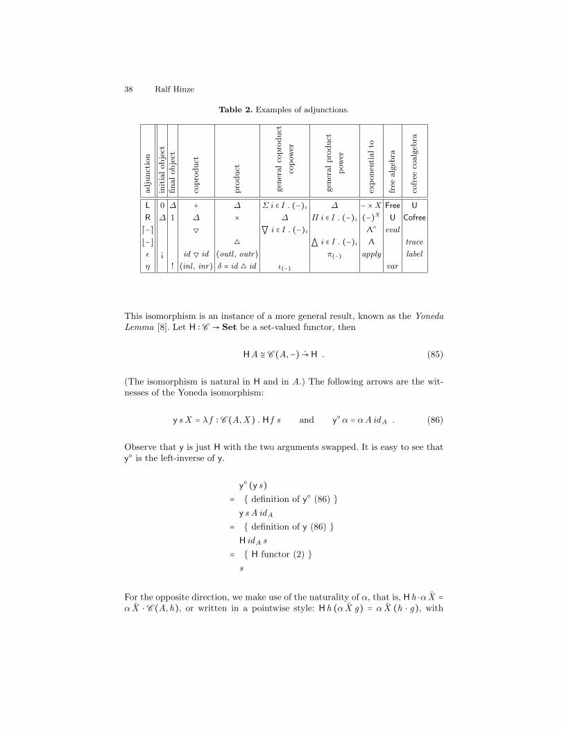
Table 2 summarises the adjunctions discussed in this section.
2.7 The Yoneda Lemma
This section introduces an important categorical tool: the Yoneda Lemma. It isrelated to continuation-passing style and induces an important proof technique,the principle of indirect proof [14].
Recall that the contravariant hom-functor C (−,X ) ∶ C op → Set maps anarrow f ∶ C (B ,A) to a function C (f ,X ) ∶ C (A,X ) → C (B ,X ). This functionis natural in X —this is the import of identity (5). Furthermore, every naturaltransformation of type C (A,−) → C (B ,−) is obtained as the image of C (f ,−)for some f . So we have the following isomorphism between arrows and naturaltransformations.
C (B ,A) ≅ C (A,−) →C (B ,−)
38 Ralf Hinze
Table 2. Examples of adjunctions.
adju
nct
ion
init
ial
ob
ject
final
ob
ject
copro
duct
pro
duct
gen
eral
copro
duct
cop
ower
gen
eral
pro
duct
pow
er
exp
onen
tial
to
free
alg
ebra
cofr
eeco
alg
ebra
L 0 ∆ + ∆ Σ i ∈ I . (−)i ∆ − ×X Free U
R ∆ 1 ∆ × ∆ Π i ∈ I . (−)i (−)X U Cofree
⌈−⌉ ▽
`i ∈ I . (−)i Λ○ eval
⌊−⌋ △
ai ∈ I . (−)i Λ trace
ε ¡ id ▽ id ⟨outl , outr⟩ π(−) apply label
η ! ⟨inl , inr⟩ δ = id △ id ι(−) var
This isomorphism is an instance of a more general result, known as the YonedaLemma [8]. Let H ∶ C → Set be a set-valued functor, then
HA ≅ C (A,−) →H . (85)
(The isomorphism is natural in H and in A.) The following arrows are the wit-nesses of the Yoneda isomorphism:
y s X = λ f ∶ C (A,X ) . H f s and y○ α = αA idA . (86)
Observe that y is just H with the two arguments swapped. It is easy to see thaty○ is the left-inverse of y.
y○ (y s)= { definition of y○ (86) }
y s A idA
= { definition of y (86) }H idA s
= { H functor (2) }s
For the opposite direction, we make use of the naturality of α, that is, Hh ⋅α X =α X ⋅ C (A,h), or written in a pointwise style: Hh (α X g) = α X (h ⋅ g), with

Generic Programming with Adjunctions 39
h ∶ C (X , X ) and g ∶ C (A, X ).
y (y○ α)X
= { definition of y (86) }λ f . H f (y○ α)
= { definition of y○ (86) }λ f . H f (αA idA)
= { α is natural: Hh (α X g) = α X (h ⋅ g) }λ f . αX (f ⋅ idA)
= { identity }λ f . αX f
= { extensionality—αX is a function }αX
For H ∶ C → Set with HX = C (B ,X ) and B fixed, we have C (B ,A) ≅C (A,−) →C (B ,−). Furthermore, the isomorphism simplifies to y g = C (g ,−) asa quick calculation shows.
y g X = λ f . C (B , f ) g = λ f . C (g ,X ) f = C (g ,X )
Conversely, for H ∶ C op → Set with HX = C (X ,B) and B fixed, we haveC (A,B) ≅ C op(A,−) →C (−,B) ≅ C (−,A) →C (−,B). Furthermore, the isomor-phism simplifies to y g = C (−, g).
These special cases give rise to the principle of indirect proof.
f = g ⇐⇒ C (f ,−) = C (g ,−) (87)
f = g ⇐⇒ C (−, f ) = C (−, g) (88)
Instead of proving the equality of f and g directly, we show the equality of theirYoneda images y f and y g .
When we discussed exponentials (see Section 2.5), we noted that there is aunique way to turn the exponential BX into a bifunctor, so that the bijection
Λ ∶ C (A ×X ,B) ≅ C (A,BX ) ∶ Λ○ (89)
is also natural in X . The proof of this fact makes essential use of the YonedaLemma. Recall that a transformation between n-ary functors is natural if andonly if it is natural in each argument separately. Let p ∶ C (X , X ), then the

40 Ralf Hinze
naturality condition (89) implies
C (−,Bp) ⋅Λ = Λ ⋅C (− × p,B)⇐⇒ { adjunction: Λ ⋅Λ○ = id and Λ○ ⋅Λ = id (27) }
C (−,Bp) = Λ ⋅C (− × p,B) ⋅Λ○
⇐⇒ { Yoneda Lemma: C (B X ,B X ) ≅ C (−,B X ) →C (−,B X ) (85) }y○ (C (−,Bp)) = y○ (Λ ⋅C (− × p,B) ⋅Λ○)
⇐⇒ { definition of y○ }
C (−,Bp)B X id = (Λ ⋅C (− × p,B) ⋅Λ○)B X id
⇐⇒ { composition of natural transformations }
C (−,Bp)B X id = (Λ ⋅C (B X × p,B) ⋅Λ○) id
⇐⇒ { definition of hom-functors (6) }
Bp = Λ (Λ○ id ⋅ (B X × p))⇐⇒ { apply = Λ○ id (Table 1) }
Bp = Λ (apply ⋅ (B X × p)) .
The reflection law (42) implies that B(−) preserves the identity. Since the natu-rality condition (89) uniquely determines B(−)’s action on arrows, it furthermorepreserves composition:
C (−,Bp⋅q)= { naturality condition (89) }
Λ ⋅C (− × (p ⋅ q),B) ⋅Λ○
= { A × − covariant functor and C (−,B) contravariant functor }Λ ⋅C (− × q ,B) ⋅C (− × p,B) ⋅Λ○
= { naturality condition (89) }Λ ⋅C (− × q ,B) ⋅Λ○ ⋅C (−,Bp)
= { naturality condition (89) and adjunction Λ ⋅Λ○ = id (27) }C (−,Bq) ⋅C (−,Bp)
= { C (A,−) covariant functor }C (−,Bq ⋅Bp) .
Applying the principle of indirect proof (88), we conclude that Bp⋅q = Bq ⋅Bp .
Exercise 35. Generalise the argument above to an arbitrary adjunction with aparameter. Let L ∶ C ← D ×X be a bifunctor, written LX A for clarity, so thatthe partial application LX ∶ C ← D has a right adjoint RX ∶ C → D for eachchoice of X ∶ X :
⌊−⌋ ∶ C (LX A,B) ≅ D(A,RX B) . (90)

Generic Programming with Adjunctions 41
1. Show that there is a unique way to turn R into a bifunctor of type X op×C →D so that the bijection (90) is natural in all three variables A, B and X .
C (LX A,B)⌊−⌋
≻ D(A,RX B)
C (LX A,B)
C (Lp A,B)
⋎
⌊−⌋≻ D(A,RX B)
D(A,Rp B)
⋎
Explain why RX is necessarily contravariant in the parameter X .2. Let ηX ∶ Id →RX ○LX be the unit of the adjunction with a parameter. What
property of η corresponds to the naturality of the bijection (90) in X ? (Theunit is not natural in X since RX ○LX is not functorial in X . Why?) ⊓⊔
3 Adjunctions for Algorithms
In the first part of these lecture notes we have seen that every fundamental ‘datastructure’ arises out of an adjunction. In the second part we turn our attention to‘algorithms’. Our goal is to give a precise semantics to a large class of recursionequations—equations as they might arise in a Haskell program.
This second part is organised as follows. Section 3.1 reviews conventionalfolds and unfolds as introduced in Section 2.6. We take a somewhat non-standardapproach and re-introduce them as solutions of so-called Mendler-style equations.Section 3.2 generalises these equations to adjoint equations and demonstratesthat many Haskell functions fall under this umbrella. Section 3.3 specialisesadjoint equations to a variety of basic adjunctions and explores the resultingrecursion schemes. Section 3.4 develops the calculational properties of adjointfolds. Like their vanilla counterparts, they enjoy reflection, computation andfusion laws.
Some knowledge of the functional programming language Haskell [15] is use-ful, as the formal development is paralleled by a series of programming examples.
3.1 Fixed-Point Equations
In this section we review the semantics of datatypes, albeit with a slight twist.The following two Haskell programs serve as running examples.
Example 1. The datatype Bush models binary leaf trees, a representation ofnon-empty sequences of natural numbers.
data Bush = Leaf Nat ∣ Fork (Bush,Bush)
The type (A,B) is Haskell syntax for the cartesian product A ×B .

42 Ralf Hinze
The function total computes the sum of a bush of natural numbers.
total ∶ Bush → Nattotal (Leaf n) = ntotal (Fork (l , r)) = total l + total r
This is a typical example of a fold, a function that consumes data. ⊓⊔
Example 2. The type Tree captures bifurcations, infinite binary trees of naturals.(A bifurcation is a division of a state or an action into two branches.)
data Tree = Branch (Tree,Nat ,Tree)
The call generate 1 constructs an infinite tree, labelled with the naturalsfrom 1 onwards.
generate ∶ Nat → Treegenerate n = Branch (generate (2 ∗ n + 0),n, generate (2 ∗ n + 1))
This is a typical example of an unfold, a function that produces data. ⊓⊔
Both the types, Bush and Tree, and the functions, total and generate, aregiven by recursion equations. At the outset, it is not at all clear that these equa-tions have solutions and if so whether the solutions are unique. It is customaryto rephrase the problem of solving recursion equations as a fixed-point problem:a recursion equation of the form x = Ψ x implicitly defines a function Ψ in theunknown x , the so-called base function of the recursion equation. A fixed-pointof the base function is then a solution of the recursion equation and vice versa.
Consider the type equation defining Bush. Its base function or, rather, itsbase functor is given by
dataBush bush = LeafNat ∣ Fork (bush, bush)instance Functor Bushwhere
fmap f (Leafn) = Leafnfmap f (Fork (l , r)) = Fork (f l , f r) .
We adopt the convention that the base functor is named after the underlyingtype, using this font for the former and this font for the latter. The type argumentof Bush marks the recursive component. In Haskell, the object part of a functoris defined by a data declaration; the arrow part is given by a Functor instance.Using arithmetic notation Bush is written BushB = Nat +B ×B .
All functors underlying first-order datatype declarations (sums of products,no function types) have two extremal fixed points: the initial F-algebra ⟨µF, in⟩and the final F-coalgebra ⟨νF, out⟩, where F ∶ C → C is the functor in question(Section 2.6). Some programming languages such as Charity [16] or Coq [17]allow the user to choose between initial and final solutions—the datatype decla-rations are flagged as inductive or coinductive. Haskell is not one of them. SinceHaskell’s underlying category is SCpo, the category of complete partial orders

Generic Programming with Adjunctions 43
and strict continuous functions, initial algebras and final coalgebras actuallycoincide [18, 19]—further background is provided at the end of this section. Incontrast, in Set elements of an inductive type are finite, whereas elements of acoinductive type are potentially infinite. Operationally, an element of an induc-tive type can be constructed in a finite sequence of steps, whereas an element ofa coinductive type allows any finite sequence of observations.
Turning to our running examples, we view Bush as an initial algebra—thoughinductive and coinductive trees are both equally useful. For bifurcations, onlythe coinductive reading is useful since in Set the initial algebra of Tree’s basefunctor is the empty set.
Definition 3. In Haskell, initial algebras and final coalgebras can be defined asfollows.
newtypeµf = In {in○ ∶ f (µf )}newtypeν f = Out○ {out ∶ f (ν f )}
The definitions use Haskell’s record syntax to introduce the destructors in○ andout in addition to the constructors In and Out○. The newtype declarationguarantees that µf and f (µf ) share the same representation at run-time, andlikewise for νf and f (νf ). In other words, the constructors and destructors areno-ops. Of course, since initial algebras and final coalgebras coincide in Haskell,they could be defined by a single newtype definition. However, since we wishto use Haskell as a meta-language for Set, we keep them separate. ⊓⊔
Working towards a semantics for total , let us first adapt its definition to thenew ‘two-level type’ µBush. The term is due to [20]; one level describes thestructure of the data, the other level ties the recursive knot.
total ∶ µBush → Nattotal (In (Leafn)) = ntotal (In (Fork (l , r))) = total l + total r
Now, if we abstract away from the recursive call, we obtain a non-recursive basefunction of type (µBush→ Nat)→ (µBush→ Nat). As with functors, we adoptthe convention that the base function is named after the underlying function,using this font for the former and this font for the latter.
total ∶ (µBush→ Nat)→ (µBush → Nat)total total (In (Leafn)) = ntotal total (In (Fork (l , r))) = total l + total r
Functions of this type possibly have many fixed points—consider as an extremeexample the identity base function, which has an infinite number of fixed points.Interestingly, the problem of ambiguity disappears into thin air, if we additionallyremove the constructor In.
total ∶ ∀x . (x → Nat)→ (Bush x → Nat)total total (Leafn) = ntotal total (Fork (l , r)) = total l + total r

44 Ralf Hinze
The type of the base function has become polymorphic in the argument of therecursive call. We shall show in the next section that this type guarantees thatthe recursive definition of total
total ∶ µBush→ Nattotal (In s) = total total s
is well-defined in the sense that the equation has exactly one solution.Applying an analogous transformation to the type Tree and the function
generate we obtain
dataTree tree =Branch (tree,Nat , tree)generate ∶ ∀x . (Nat → x)→ (Nat → Tree x)generate generate n
=Branch (generate (2 ∗ n + 0),n, generate (2 ∗ n + 1))generate ∶ Nat → νTreegenerate n = Out○ (generate generate n) .
Again, the base function enjoys a polymorphic type that guarantees that therecursive function is well-defined.
Abstracting away from the particulars of the syntax, the examples suggestthe consideration of fixed-point equations of the form
x ⋅ in = Ψ x , and dually out ⋅ x = Ψ x , (91)
where the unknown x has type C (µF,A) on the left and C (A, νG) on the right.The Haskell definitions above are pointwise versions of these equations: x (In a) =Ψ x a and x a = Out○ (Ψ x a). Arrows defined by equations of this form are knownas Mendler-style folds and unfolds, because they were originally introduced byMendler [21] in the setting of type theory. We shall usually drop the qualifierand call the solutions simply folds and unfolds. In fact, the abuse of language isjustified as each Mendler-style equation is equivalent to the defining equation ofa standard (un)fold. This is what we show next, considering folds first.
3.1.1 Initial Fixed-Point Equations. Let C be some base category and letF ∶ C → C be some endofunctor. An initial fixed-point equation in the unknownx ∶ C (µF,A) has the syntactic form
x ⋅ in = Ψ x , (92)
where the base function Ψ has type
Ψ ∶ ∀X . C (X ,A)→ C (FX ,A) .
In the fixed-point equation (92) the natural transformation Ψ is instantiated tothe initial algebra: x ⋅in = Ψ (µF) x . For reasons of readability we will usually omit

Generic Programming with Adjunctions 45
the ‘type arguments’ of natural transformations. The diagram below displays thetypes involved.
F (µF)
µF
in
⋎x
≻ A
Ψ (µF) x
≻
The naturality condition can be seen as the semantic counterpart of theguarded-by-destructors condition [22]. This becomes visible if we move the iso-morphism in ∶ F (µF) ≅ µF to the right-hand side: x = Ψ x ⋅ in○. Here in○ is thedestructor that guards the recursive calls. The equation has a straightforwardoperational reading. The argument of x is destructed yielding an element of typeF (µF). The base function Ψ then works on the F-structure, possibly applying itsfirst argument, the recursive call of x , to elements of type µF. These elementsare proper sub-terms of the original argument—recall that the type argument ofF marks the recursive components. The naturality of Ψ ensures that only thesesub-terms can be passed to the recursive calls.
Does this imply that x is terminating? Termination is an operational notion;how the notion translates to a denotational setting depends on the underlyingcategory. Our primary goal is to show that Equation (92) has a unique solution.When working in Set this result implies that the equation admits a solution thatis indeed a total function. Furthermore, the operational reading of x = Ψ x ⋅ in○
suggests that x is terminating, as elements of an inductive type can only bedestructed a finite number of times. (Depending on the evaluation strategy thisclaim is also subject to the proviso that the F-structures themselves are finite.)On the other hand, if the underlying category is SCpo, then the solution is acontinuous function that does not necessarily terminate for all its inputs, sinceinitial algebras in SCpo possibly contain infinite elements.
While the definition of total fits nicely into the framework above, the followingprogram does not.
Example 4. The naturality condition is sufficient but not necessary as the ex-ample of the binary increment demonstrates.
data Nat = N ∣ O Nat ∣ I Nat
succ ∶ Nat → Natsucc (N ) = I Nsucc (O b) = I bsucc (I b) = O (succ b)
As with total , we split the datatype into two levels.
type Nat = µNat
dataNatnat =N ∣ Onat ∣ Inat

46 Ralf Hinze
instance Functor Natwherefmap f (N) =Nfmap f (O b) =O (f b)fmap f (I b) = I (f b)
In Set, the implementation of the successor function is clearly terminating. How-ever, the associated base function
succ ∶ (Nat → Nat)→ (NatNat → Nat)succ succ (N) = In (I (In N))succ succ (O b) = In (I b)succ succ (I b) = In (O (succ b))
lacks naturality. In a sense, its type is too concrete, as it reveals that the recursivecall is passed a binary number. An adversary can make use of this informationturning the terminating program into a non-terminating one:
bogus ∶ (Nat → Nat)→ (NatNat → Nat)bogus succ (N) = In (I (In N))bogus succ (O b) = In (I b)bogus succ (I b) = succ (In (I b)) .
We will get back to this example in Section 3.3.2 (Example 19). ⊓⊔
Turning to the proof of uniqueness, let us spell out the naturality propertyof the base function Ψ . If h ∶ C (X1,X2), then C (Fh, id) ⋅Ψ = Ψ ⋅C (h, id). Usingthe definition of hom-functors (6), this unfolds to
Ψ f ⋅ Fh = Ψ (f ⋅ h) , (93)
for all arrows f ∶ C (X2,A). This property implies, in particular, that Ψ is com-pletely determined by its image of id as Ψ h = Ψ id ⋅ Fh. Now, to prove thatequation x ⋅ in = Ψ x (92) has a unique solution, we show that x is a solution ifand only if x is a standard fold.
x ⋅ in = Ψ x
⇐⇒ { Ψ is natural (93) }x ⋅ in = Ψ id ⋅ F x
⇐⇒ { uniqueness property of standard folds (54) }x = ((Ψ id ))
Overloading the banana brackets, the unique solution of the fixed-point equationx ⋅ in = Ψ x (92) is written ((Ψ )).
Let us explore the relation between standard folds and Mendler-style folds inmore depth. The proof above rests on the fact that the type of Ψ is isomorphicto C (FA,A), the type of F-algebras.
C (FA,A) ≅ (∀X ∶ C . C (X ,A)→ C (FX ,A)) .

Generic Programming with Adjunctions 47
This bijection between arrows and natural transformations is an instance of theYoneda Lemma (Section 2.7), where the contravariant functor H ∶ C op → Setis given by H = C (F−,A). Consequently, Mendler-style folds and standard foldsare related by ((Ψ )) = ((y○ Ψ )) = ((Ψ id )) and ((λ x . a ⋅ F x )) = ((y a )) = ((a )).
Example 1. The standard fold for computing the total of a bush of natural num-bers is ((id ▽ plus )), see Section 2.6.1. Written in a pointwise style, the algebraid ▽ plus reads
total ∶BushNat → Nattotal (Leafn) = ntotal (Fork (l , r)) = l + r .
The algebra and the base function are related by total = total id and total total =total ⋅ fmap total , which implies ((total)) = ((total)). ⊓⊔
3.1.2 Final Fixed-Point Equations. The development of the previous sec-tion dualises to final coalgebras. For completeness, let us spell out the details.
A final fixed-point equation in the unknown x ∶ C (A, νG) has the form
out ⋅ x = Ψ x , (94)
where the base function Ψ has type
Ψ ∶ ∀X . C (A,X )→ C (A,GX ) .
Overloading the lens brackets, the unique solution of (94) is denoted [(Ψ )].In Set, the naturality condition captures the guarded-by-constructors condi-
tion [22] ensuring productivity. Again, this can be seen more clearly if we movethe isomorphism out ∶ νG ≅ G (νG) to the right-hand side: x = out○ ⋅ Ψ x . Hereout○ is the constructor that guards the recursive calls. The base function Ψ has toproduce a G (νG) structure. To create the recursive components of type νG, thebase function Ψ can use its first argument, the recursive call of x . However, thenaturality of Ψ ensures that these calls can only be made in guarded positions.
The type of Ψ is isomorphic to C (A,GA), the type of G-coalgebras.
C (A,GA) ≅ (∀X ∶ C . C (A,X )→ C (A,GX )) .
Again, this is an instance of the Yoneda Lemma: now H = C (A,G−) is a covariantfunctor H ∶ D → Set.
Example 2. The standard unfold for constructing an infinite tree of natural num-bers is [(shift0 △ id △ shift1 )], see Section 2.6.2. Written in a pointwise style, thecoalgebra shift0 △ id △ shift1 reads
generate ∶ Nat → TreeNatgenerate n = Branch (2 ∗ n + 0,n,2 ∗ n + 1) .
The coalgebra and the base function are related by generate = generate id andgenerate gen = fmap gen ⋅ generate, which implies [(generate)] = [(generate)]. ⊓⊔
In the following sections we show that fixed-point equations are quite general.More functions fit under this umbrella than one might initially think.

48 Ralf Hinze
3.1.3 Mutual Type Recursion. In Haskell, datatypes can be defined bymutual recursion.
Example 5. Imagine a simple imperative programming language. The abstractsyntax of expressions and statements is typically defined by mutual type recur-sion (this is a very stripped-down example).
data Expr = Var Var ∣ Block (Stat ,Expr)data Stat = Assign (Var ,Expr) ∣ Seq (Stat ,Stat)
As function follows form, functions that consume an abstract syntax tree aretypically defined by mutual value recursion.
type Vars = SetVar
varsExpr ∶ Expr → VarsvarsExpr (Var x) = {x}varsExpr (Block (s, e)) = varsStat s ∪ varsExpr e
varsStat ∶ Stat → VarsvarsStat (Assign (x , e)) = {x} ∪ varsExpr evarsStat (Seq (s1, s2)) = varsStat s1 ∪ varsStat s2
The functions determine the variables of either an expression or a statement,assuming a suitable collection type Set with operations {−} and ∪. ⊓⊔Can we fit the above definitions into the framework of the previous section? Yes,we only have to choose a suitable base category: in this case, a product category(Section 2.2.2). The base functor underlying Expr and Stat is an endofunctorover a product category:
Grammar ⟨A, B⟩ = ⟨Var +B ×A, Var ×A +B ×B⟩ .The Haskell types Expr and Stat are then the components of the fixed point:µGrammar = ⟨Expr , Stat⟩. The functions varsExpr and varsStat are handledaccordingly: we bundle them to a single arrow
vars = ⟨varsExpr , varsStat⟩ ∶ (C ×C )(µGrammar, ⟨Vars, Vars⟩) .
The following calculation makes explicit that an initial fixed-point equationin C ×D corresponds to two equations, one in C and one in D .
x ⋅ in = Ψ x ∶ (C ×D)(F (µF), ⟨A1, A2⟩)⇐⇒ { surjective pairing: f = ⟨Outl f , Outr f ⟩ }
⟨Outl x , Outr x ⟩ ⋅ ⟨Outl in, Outr in⟩ = Ψ ⟨Outl x , Outr x ⟩⇐⇒ { set x1 = Outl x , x2 = Outr x and in1 = Outl in, in2 = Outr in }
⟨x1, x2⟩ ⋅ ⟨in1, in2⟩ = Ψ ⟨x1, x2⟩⇐⇒ { definition of composition in C ×D }
⟨x1 ⋅ in1, x2 ⋅ in2⟩ = Ψ ⟨x1, x2⟩⇐⇒ { surjective pairing: f = ⟨Outl f , Outr f ⟩ }
⟨x1 ⋅ in1, x2 ⋅ in2⟩ = ⟨Outl (Ψ ⟨x1, x2⟩), Outr (Ψ ⟨x1, x2⟩)⟩

Generic Programming with Adjunctions 49
⇐⇒ { set Ψ1 = Outl○Ψ and Ψ2 = Outr○Ψ }⟨x1 ⋅ in1, x2 ⋅ in2⟩ = ⟨Ψ1 ⟨x1, x2⟩, Ψ2 ⟨x1, x2⟩⟩
⇐⇒ { equality of arrows in C ×D }x1 ⋅ in1 = Ψ1 ⟨x1, x2⟩ ∶ C (Outl (F (µF)),A1) and
x2 ⋅ in2 = Ψ2 ⟨x1, x2⟩ ∶ D(Outr (F (µF)),A2)
The base functions Ψ1 and Ψ2 are parametrised both with x1 and x2. Other thanthat, the syntactic form is identical to a standard fixed-point equation.
It is a simple exercise to bring the equations of Example 5 into this form:
Definition 6. In Haskell, mutually recursive types can be modelled as follows.
newtypeµ1 f1 f2 = In1 {in○1 ∶ f1 (µ1 f1 f2) (µ2 f1 f2)}
newtypeµ2 f1 f2 = In2 {in○2 ∶ f2 (µ1 f1 f2) (µ2 f1 f2)}
Since Haskell has no concept of pairs on the type level, that is, no product kinds,we have to curry the type constructors: µ1 f1 f2 = Outl (µ⟨f1, f2⟩) and µ2 f1 f2 =Outr (µ⟨f1, f2⟩). ⊓⊔
Example 7. The base functors of Expr and Stat are
dataExpr expr stat =VarVar ∣ Block (stat , expr)dataStat expr stat = Assign (Var , expr) ∣ Seq (stat , stat) .
Since all Haskell functions live in the same category, we have to represent arrowsin C ×C by pairs of arrows in C .
varsExpr ∶ ∀x1 x2 .(x1 → Vars, x2 → Vars)→ (Expr x1 x2 → Vars)
varsExpr (varsExpr , varsStat) (Var x) = {x}varsExpr (varsExpr , varsStat) (Block (s, e)) = varsStat s ∪ varsExpr e
varsStat ∶ ∀x1 x2 .(x1 → Vars, x2 → Vars)→ (Stat x1 x2 → Vars)
varsStat (varsExpr , varsStat) (Assign (x , e)) = {x} ∪ varsExpr evarsStat (varsExpr , varsStat) (Seq (s1, s2)) = varsStat s1 ∪ varsStat s2
The definitions of varsExpr and varsStat match exactly the scheme above.
varsExpr ∶ µ1 ExprStat→ VarsvarsExpr (In1 e) = varsExpr (varsExpr , varsStat) e
varsStat ∶ µ2 ExprStat→ VarsvarsStat (In2 s) = varsStat (varsExpr , varsStat) s
Since the two equations are equivalent to an initial fixed-point equation in C ×C ,they indeed have unique solutions. ⊓⊔

50 Ralf Hinze
No new theory is needed to deal with mutually recursive datatypes and mutuallyrecursive functions over them. By duality, the same is true for final coalgebras.For final fixed-point equations we have the following correspondence.
out ⋅ x = Ψ x ⇐⇒ out1 ⋅ x1 = Ψ1 ⟨x1, x2⟩ and out2 ⋅ x2 = Ψ2 ⟨x1, x2⟩
3.1.4 Type Functors. In Haskell, datatypes can be parametrised by types.
Example 8. The type of random-access lists [23] is given by
dataArray a = Null ∣ Zero (Array (a,a)) ∣ One (a,Array (a,a))instance Functor Arraywhere
fmap f (Null) = Nullfmap f (Zero s) = Zero (fmap (f × f ) s)fmap f (One (a, s)) = One (f a, fmap (f × f ) s)
(×) ∶ (a→ a)→ (b→ b)→ ((a, b)→ (a, b))(f × g) (a, b) = (f a, g b) .
The type Array is a so-called nested datatype [24] as the type argument changesfrom a to (a,a) in the recursive calls. Random-access lists are a numerical rep-resentation, a container type that is modelled after a number system, here thebinary numbers.
size ∶ ∀a . Array a → Natsize (Null) = 0size (Zero s) = 2 ∗ size s + 0size (One (a, s)) = 2 ∗ size s + 1
The function size calculates the size of a random-access list, illustrating the cor-respondence between random-access lists and binary numbers. The definition re-quires polymorphic recursion [25], as the recursive calls have type Array (a,a)→Nat , which is a substitution instance of the declared type. ⊓⊔
Can we fit the definitions above into the framework of Section 3.1.1? Again,the answer is yes. We only have to choose a suitable base category: this time,a functor category (Section 2.2.3). The base functor of Array is an endofunctorover a functor category:
ArrayFA = 1 + F (A ×A) +A × F (A ×A) .
The second-order functor Array sends a functor to a functor. Since its fixed pointArray = µArray lives in a functor category, folds over random-access lists are nec-essarily natural transformations. The function size is a natural transformation,as we can assign it the type
size ∶ µArray →KNat ,
where K ∶ D → DC is the constant functor defined KA B = A. Again, we canreplay the development in Haskell.

Generic Programming with Adjunctions 51
Definition 9. The definition of second-order initial algebras and final coalgebrasis identical to that of Definition 3, except for an additional type argument.
newtypeµf a = In {in○ ∶ f (µf )a }newtypeν f a = Out○ {out ∶ f (ν f )a }
To capture the fact that µf and νf are functors whenever f is a second-orderfunctor, we need an extension of the Haskell 2010 class system.
instance (∀x . (Functor x)⇒ Functor (f x))⇒ Functor (µf )wherefmap f (In s) = In (fmap f s)
instance (∀x . (Functor x)⇒ Functor (f x))⇒ Functor (νf )wherefmap f (Out○ s) = Out○ (fmap f s)
The declarations use a so-called polymorphic predicate [26], which precisely cap-tures the requirement that f sends functors to functors. Unfortunately, the exten-sion has not been implemented yet. It can be simulated within Haskell 2010 [27],but the resulting code is somewhat clumsy. Alternatively, one can use ‘recursivedictionaries’
instance Functor (f (µf ))⇒ Functor (µf )wherefmap f (In s) = In (fmap f s)
instance Functor (f (νf ))⇒ Functor (νf )wherefmap f (Out○ s) = Out○ (fmap f s)
and rely on the compiler to tie the recursive knot [28]. ⊓⊔
Let us specialise fixed-point equations to functor categories.
x ⋅ in = Ψ x
⇐⇒ { equality of arrows in DC }∀A ∶ C . (x ⋅ in)A = Ψ x A
⇐⇒ { definition of composition in DC }∀A ∶ C . x A ⋅ in A = Ψ x A
In Haskell, type application is invisible, so fixed-point equations in functor cat-egories cannot be distinguished from equations in the base category.
Example 10. Continuing Example 8, the base functor of Array maps functors tofunctors: it has kind (⋆→ ⋆)→ (⋆→ ⋆).
dataArrayarray a =Null ∣ Zero (array (a,a)) ∣ One (a,array (a,a))instance (Functor array)⇒ Functor (Arrayarray)where
fmap f (Null) =Nullfmap f (Zero s) = Zero (fmap (f × f ) s)fmap f (One (a, s)) =One (f a, fmap (f × f ) s)

52 Ralf Hinze
Table 3. Initial algebras and final coalgebras in different categories.
categoryinitial fixed-point equation final fixed-point equation
x ⋅ in = Ψ x out ⋅ x = Ψ x
Setinductive type coinductive typestandard fold standard unfold
Cpo —continuous coalgebra (domain)
continuous unfold(F locally continuous in SCpo)
SCpocontinuous algebra (domain) continuous coalgebra (domain)
strict continuous fold strict continuous unfold(F locally continuous in SCpo, µF ≅ νF)
C ×D
mutually recursive inductive types mutually recursive coinductive typesmutually recursive folds mutually recursive unfolds
x1 ⋅ in1 = Ψ1 ⟨x1, x2⟩ out1 ⋅ x1 = Ψ1 ⟨x1, x2⟩x2 ⋅ in2 = Ψ2 ⟨x1, x2⟩ out2 ⋅ x2 = Ψ2 ⟨x1, x2⟩
DCinductive type functor coinductive type functor
higher-order fold higher-order unfoldx A ⋅ in A = Ψ x A out A ⋅ x A = Ψ x A
Its action on arrows, not shown above, maps natural transformations to naturaltransformations. Accordingly, the base function of size is a second-order naturaltransformation that takes natural transformations to natural transformations.
size ∶ ∀x . (∀a . x a → Nat)→ (∀a . Array x a → Nat)size size (Null) = 0size size (Zero s) = 2 ∗ size s + 0size size (One (a, s)) = 2 ∗ size s + 1
size ∶ ∀a . µArraya → Natsize (In s) = size size s
The resulting equation fits the pattern of an initial fixed-point equation (typeapplication is invisible in Haskell). Consequently, it has a unique solution. ⊓⊔
Table 3 summarises our findings so far. To provide some background, Cpois the category of complete partial orders and continuous functions; SCpo isthe full subcategory of strict functions. A functor F ∶ SCpo → SCpo is locallycontinuous if its action on arrows SCpo(A,B)→ SCpo(FA,FB) is continuousfor any pair of objects A and B . A continuous algebra is just an algebra whosecarrier is a complete partial order and whose action is a continuous function. InSCpo, every locally continuous functor has an initial algebra and, furthermore,the initial algebra coincides with the final coalgebra. This is the reason whySCpo is commonly considered to be Haskell’s ambient category. It may seemodd at first that lazy programs are modelled by strict functions. Non-strict func-tions, however, are in one-to-one correspondence to strict functions from a lifteddomain: SCpo(A�,B) ≅ Cpo(A,B). (In other words, we have an adjunction

Generic Programming with Adjunctions 53
(−)� ⊣ Incl between lifting and the inclusion functor Incl ∶ SCpo → Cpo.) Thedenotational notion of lifting, adding a new least element, models the operationalnotion of a thunk (also known as a closure, laze or recipe).
3.2 Adjoint Fixed-Point Equations
We have seen in the previous section that initial and final fixed-point equationsare quite general. However, there are obviously a lot of definitions that do notfit the pattern. We have mentioned list concatenation and others in the intro-duction.
Example 11. The datatype Stack models stacks of natural numbers.
data Stack = Empty ∣ Push (Nat ,Stack)
The function cat concatenates two stacks.
cat ∶ (Stack , Stack)→ Stackcat (Empty , ns) = nscat (Push (m,ms),ns) = Push (m, cat (ms,ns))
The definition does not fit the pattern of an initial fixed-point equation as ittakes two arguments and recurses only over the first one. ⊓⊔Example 12. The functions left and right generate infinite trees labelled withzeros and ones.
left ∶ ()→ Treeleft () = Branch (left (),0, right ())right ∶ ()→ Treeright () = Branch (left (),1, right ())
The two definitions are not instances of final fixed-point equations, because eventhough the functions are mutually recursive the datatype is not. ⊓⊔
In Example 11 the element of the initial algebra is embedded in a context.Written in a point-free style the definition of cat is of the form x ⋅(in × id) = Ψ x .The central idea of these lecture notes is to model this context by a functor,generalising fixed-point equations to
x ⋅ L in = Ψ x , and dually Rout ⋅ x = Ψ x , (95)
where the unknown x has type C (L (µF),A) on the left and C (A,R (νG)) onthe right. The functor L models the context of µF. In the case of cat the functoris L = − × Stack . Dually, R allows x to return an element of νG embedded in acontext. Section 3.3.2 discusses a suitable choice for R in Example 12.
Of course, the functors L and R cannot be arbitrary. For instance, for L = KAwhere K ∶ C → C D is the constant functor and Ψ = id , the equation x ⋅ L in = Ψ xsimplifies to x = x , which every arrow of the appropriate type satisfies. Oneapproach for ensuring uniqueness is to require L and R to be adjoint: L ⊣ R(Section 2.5). The adjoint transposition allows us to trade L in the source for Rin the target of an arrow, which is the key for showing that generalised fixed-point equations (95) have unique solutions. This is what we do next.

54 Ralf Hinze
3.2.1 Adjoint Initial Fixed-Point Equations. Let C and D be categories,let L ⊣ R be an adjoint pair of functors L ∶ C ← D and R ∶ C → D , and letF ∶ D → D be some endofunctor. An adjoint initial fixed-point equation in theunknown x ∶ C (L (µF),A) has the syntactic form
x ⋅ L in = Ψ x , (96)
where the base function Ψ has type
Ψ ∶ ∀X ∶ D . C (LX ,A)→ C (L (FX ),A) .
The unique solution of (96) is called an adjoint fold, denoted ((Ψ ))L. The diagramsbelow summarise the type information.
L (F (µF))
L (µF)
L in
⋎
x≻ A
Ψ (µF) x
≻
C
R//� D
LooF
xx
The proof of uniqueness makes essential use of the fact that the left adjunctis natural in A.
x ⋅ L in = Ψ x
⇐⇒ { adjunction: ⌈⌊f ⌋⌉ = f (27) }⌊x ⋅ L in⌋ = ⌊Ψ x ⌋
⇐⇒ { fusion: ⌊−⌋ is natural in A (37) }⌊x ⌋ ⋅ in = ⌊Ψ x ⌋
⇐⇒ { adjunction: ⌈⌊f ⌋⌉ = f }⌊x ⌋ ⋅ in = ⌊Ψ ⌈⌊x ⌋⌉⌋
⇐⇒ { Section 3.1.1 }⌊x ⌋ = ((λ x . ⌊Ψ ⌈x ⌉⌋))
⇐⇒ { adjunction: f = ⌈g⌉⇐⇒ ⌊f ⌋ = g (27) }x = ⌈((λ x . ⌊Ψ ⌈x ⌉⌋))⌉
In three simple steps we have transformed the adjoint fold x ∶ C (L (µF),A)into the standard fold ⌊x ⌋ ∶ D(µF,RA) and, alongside, the adjoint base func-tion Ψ ∶ ∀X . C (LX ,A) → C (L (FX ),A) into the standard base functionλ x . ⌊Ψ ⌈x ⌉⌋ ∶ ∀X . D(X ,RA) → D(FX ,RA). We have shown in Section 3.1.1that the resulting equation has a unique solution. To summarise,
((Ψ ))L = ⌈((λ x . ⌊Ψ ⌈x ⌉⌋))⌉ or, equivalently, ⌊((Ψ ))L⌋ = ((λ x . ⌊Ψ ⌈x ⌉⌋)) .
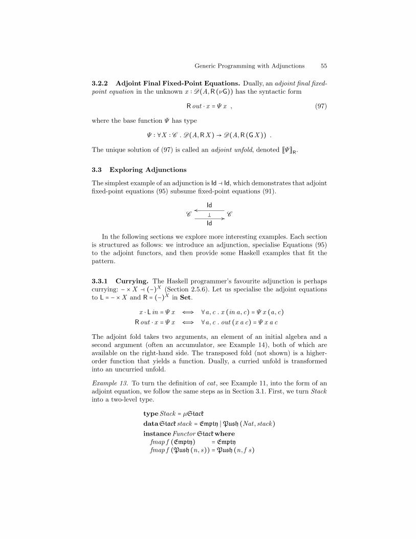
Generic Programming with Adjunctions 55
3.2.2 Adjoint Final Fixed-Point Equations. Dually, an adjoint final fixed-point equation in the unknown x ∶ D(A,R (νG)) has the syntactic form
Rout ⋅ x = Ψ x , (97)
where the base function Ψ has type
Ψ ∶ ∀X ∶ C . D(A,RX )→ D(A,R (GX )) .
The unique solution of (97) is called an adjoint unfold, denoted [(Ψ )]R.
3.3 Exploring Adjunctions
The simplest example of an adjunction is Id ⊣ Id, which demonstrates that adjointfixed-point equations (95) subsume fixed-point equations (91).
C≺
Id
�Id
≻ C
In the following sections we explore more interesting examples. Each sectionis structured as follows: we introduce an adjunction, specialise Equations (95)to the adjoint functors, and then provide some Haskell examples that fit thepattern.
3.3.1 Currying. The Haskell programmer’s favourite adjunction is perhapscurrying: − × X ⊣ (−)X (Section 2.5.6). Let us specialise the adjoint equationsto L = − ×X and R = (−)X in Set.
x ⋅ L in = Ψ x ⇐⇒ ∀a, c . x (in a, c) = Ψ x (a, c)Rout ⋅ x = Ψ x ⇐⇒ ∀a, c . out (x a c) = Ψ x a c
The adjoint fold takes two arguments, an element of an initial algebra and asecond argument (often an accumulator, see Example 14), both of which areavailable on the right-hand side. The transposed fold (not shown) is a higher-order function that yields a function. Dually, a curried unfold is transformedinto an uncurried unfold.
Example 13. To turn the definition of cat , see Example 11, into the form of anadjoint equation, we follow the same steps as in Section 3.1. First, we turn Stackinto a two-level type.
type Stack = µStack
dataStack stack = Empty ∣ Push (Nat , stack)instance Functor Stackwhere
fmap f (Empty) = Emptyfmap f (Push (n, s)) =Push (n, f s)

56 Ralf Hinze
Second, we determine the base function abstracting away from the recursive call,additionally removing in, and then we tie the recursive knot (L = − × Stack).
cat ∶ ∀x . (L x → Stack)→ (L (Stack x) → Stack)cat cat (Empty, ns) = nscat cat (Push (m,ms),ns) = Push (m, cat (ms,ns))cat ∶ LStack → Stackcat (In ms,ns) = cat cat (ms,ns)
The defining equation fits the pattern of an adjoint initial fixed-point equation,x ⋅ (in × id) = Ψ x . Since L = −×Stack has a right adjoint, cat is uniquely defined.The transposed fold, cat ′ = ⌊cat⌋,
cat ′ ∶ Stack → RStackcat ′ (In Empty) = λns → nscat ′ (In (Push (m,ms))) = λns → Push (m, (cat ′ ms)ns)
is simply the curried variant of cat . ⊓⊔
Example 14. The function shunt pushes the elements of the first onto the secondstack.
shunt ∶ (µStack, Stack)→ Stackshunt (In Empty, ns) = nsshunt (In (Push (m,ms)),ns) = shunt (ms,Push (m,ns))
Unlike cat , the parameter of shunt is changed in the recursive call—it serves asan accumulator. Nonetheless, shunt fits into the framework, as its base function
shunt ∶ ∀x . (L x → Stack)→ (L (Stack x) → Stack)shunt shunt (Empty, ns) = nsshunt shunt (Push (m,ms),ns) = shunt (ms,Push (m,ns))
has the required naturality property. The revised definition of shunt
shunt ∶ L (µStack) → Stackshunt (In ms,ns) = shunt shunt (ms,ns)
matches exactly the scheme for adjoint initial fixed-point equations. ⊓⊔
Exercise 36. Is the following tail-recursive variant of total (see Example 1)
totalPlus ∶ (Bush,Nat) → NattotalPlus (Leaf n, s) = n + stotalPlus (Fork (l , r), s) = totalPlus (l , totalPlus (r , s))
an adjoint fold? ⊓⊔
Lists are parametric in Haskell. Can we adopt the above reasoning to para-metric types and polymorphic functions?

Generic Programming with Adjunctions 57
Example 15. The type of lists is given as the initial algebra of a higher-orderbase functor of kind (⋆→ ⋆)→ (⋆→ ⋆).
typeList = µListdataList list a =Nil ∣ Cons (a, list a)instance (Functor list)⇒ Functor (List list)where
fmap f Nil =Nilfmap f (Cons (a,as)) = Cons (f a, fmap f as)
(Again, we do not need the functor’s action on arrows, which maps naturaltransformations to natural transformations.) Lists generalise stacks, sequencesof natural numbers, to an arbitrary element type. Likewise, the function
append ∶ ∀a . (µLista, Lista)→ Listaappend (In Nil, bs) = bsappend (In (Cons (a,as)), bs) = In (Cons (a,append (as, bs)))
generalises cat (Example 11) to sequences of an arbitrary element type. ⊓⊔
If we lift products pointwise to functors, (F × G)A = FA × GA, we can viewappend as a natural transformation of type
append ∶ List × List → List .
All that is left to do is to find the right adjoint of the lifted product − ×H. Onecould be led to think that F × H → G ≅ F → (H → G), but this does not workas H → G is not a functor in any sensible way (recall that H → G is the set ofnatural transformations from H to G). Also, lifting exponentials pointwise GH A =(GA)HA does not work, because again the data does not define a functor as theexponential is contravariant in its first argument. To make progress, let us assumethat the functor category is SetC so that GH ∶ C → Set. (The category SetC op
ofcontravariant, set-valued functors and natural transformations is known as thecategory of pre-sheaves.) We reason as follows:
GH A
≅ { Yoneda Lemma (85) }C (A,−) →GH
≅ { requirement: − ×H ⊣ (−)H }C (A,−) ×H →G .
The derivation suggests that the exponential of the functors H and G is givenby C (A,−) × H → G. However, the calculation does not prove that the functorthus defined is actually right adjoint to − ×H, as its existence is assumed in thesecond step. We leave the proof as a (laborious) exercise to the reader—a moregeneral result abstracting away from Set can be found in [11].
Exercise 37. Show that − ×H is left adjoint to (−)H.

58 Ralf Hinze
1. Show that GH A = C (A,−) ×H →G is functorial in A. (The functor GH takesan object to a set of natural transformations and an arrow to a function thatin turn takes a natural transformation to a natural transformation.)
2. The adjuncts of − ×H ⊣ (−)H are defined
⌊σ⌋ = λA . λ s . λX . λ (k , t) . σX (F k s, t) ,
⌈τ⌉ = λA . λ (s, t) . τ A s A (id , t) .
Prove that they are natural in F and G and mutually inverse. ⊓⊔
∗ Exercise 38. Can you make sense of the functors IdId and IdSq? ⊓⊔
Definition 16. The definition of exponentials goes beyond Haskell 2010, as itrequires rank-2 types (the data constructor Exp has a rank-2 type).
newtypeExph g a = Exp {exp○ ∶ ∀x . (a → x ,h x)→ g x }instance Functor (Exph g)where
fmap f (Exp h) = Exp (λ(k , t)→ h (k ⋅ f , t))
Morally, h and g are functors, as well. However, their mapping functions are notneeded to define the Exph g instance of Functor . The adjuncts are defined
⌊−⌋Exp ∶ (Functor f )⇒ (∀x . (f x ,h x)→ g x)→ (∀x . f x → Exph g x)⌊σ⌋Exp = λs → Exp (λ(k , t)→ σ (fmap k s, t))⌈−⌉Exp ∶ (∀x . f x → Exph g x)→ (∀x . (f x ,h x)→ g x)⌈τ⌉Exp = λ(s, t)→ exp○ (τ s) (id , t) .
The type variables f , g and h are implicitly universally quantified. Again, mostof the functor instances are not needed. ⊓⊔
Example 17. Continuing Example 15, we may conclude that the defining equa-tion of append has a unique solution. Its transpose of type List →ListList is inter-esting as it combines append with fmap:
append ′ ∶ ∀a . Lista → ∀x . (a → x)→ (List x → List x)append ′ as = λf → λbs → append (fmap f as, bs) .
For clarity, we have inlined the definition of ExpList List. ⊓⊔
3.3.2 Mutual Value Recursion. The functions left and right introducedin Example 12 are defined by mutual recursion. The program is similar to Ex-ample 5, which defines varsExpr and varsStat , with the notable difference thatonly one datatype is involved, rather than a pair of mutually recursive datatypes.Nonetheless, the correspondence suggests to view left and right as a single arrowin a product category.
trees ∶ ⟨1, 1⟩→∆(νTree)The arrow trees is an adjoint unfold since the diagonal functor ∆ ∶ C → C ×C hasa left adjoint, the coproduct (Sections 2.3.2 and 2.5.1). Using a similar reasoning

Generic Programming with Adjunctions 59
as in Section 3.1.3, we can unfold the adjoint final fixed-point equation specialisedto the diagonal functor:
∆out ⋅ x = Ψ x ⇐⇒ out ⋅ x1 = Ψ1 ⟨x1, x2⟩ and out ⋅ x2 = Ψ2 ⟨x1, x2⟩ ,
where x1 = Outl x , x2 = Outr x , Ψ1 = Outl○Ψ and, Ψ2 = Outr○Ψ . The resultingequations are similar to those of Section 3.1.3, except that now the destructorout is the same in both equations.
Example 18. Continuing Example 12, the base functions of left and right aregiven by
left ∶ ∀x . (()→ x , ()→ x)→ (()→ Tree x)left (left , right) () = Branch (left (),0, right ())right ∶ ∀x . (()→ x , ()→ x)→ (()→ Tree x)right (left , right) () = Branch (left (),1, right ()) .
The recursion equations
left ∶ ()→ νTreeleft () = Out○ (left (left , right) ())right ∶ ()→ νTreeright () = Out○ (right (left , right) ())
exactly fit the pattern above (if we move Out○ to the left-hand side). Hence,both functions are uniquely defined. Their transpose, ⌈⟨left , right⟩⌉, combinesthe two functions into a single one using a coproduct.
trees ∶ Either () ()→ νTreetrees (Left ()) = Out○ (Branch (trees (Left ()),0, trees (Right ())))trees (Right ()) = Out○ (Branch (trees (Left ()),1, trees (Right ())))
The predefined datatype Either given by dataEither a b = Left a ∣ Right b isHaskell’s coproduct. ⊓⊔
Let us turn to the dual case. To handle folds defined by mutual recursion, weneed the right adjoint of the diagonal functor, which is the product (Sections 2.3.1and 2.5.1). Specialising the adjoint initial fixed-point equation yields
⟨x1, x2⟩ ⋅∆in = Ψ ⟨x1, x2⟩ ⇐⇒ x1 ⋅ in = Ψ1 ⟨x1, x2⟩ and x2 ⋅ in = Ψ2 ⟨x1, x2⟩ .
Example 19. We can use mutual value recursion to fit the definition of the binaryincrement (Example 4) into the framework. The definition of succ has the formof a paramorphism [29], as the argument that drives the recursion is not exclu-sively used in the recursive call. The idea is to ‘guard’ the other occurrence bythe identity function and to pretend that both functions are defined by mutualrecursion.

60 Ralf Hinze
succ ∶ µNat → Natsucc (In (N)) = In (I (In N))succ (In (O b)) = In (I (id b))succ (In (I b)) = In (O (succ b))
id ∶ µNat → Natid (In (N)) = In (N)id (In (O b)) = In (O (id b))id (In (I b)) = In (I (id b))
If we abstract away from the recursive calls, we find that the two base func-tions have indeed the required polymorphic types.
succ ∶ ∀x . (x → Nat , x → Nat)→ (Nat x → Nat)succ (succ, id) (N) = In (I (In N))succ (succ, id) (O b) = In (I (id b))succ (succ, id) (I b) = In (O (succ b))id ∶ ∀x . (x → Nat , x → Nat)→ (Nat x → Nat)id (succ, id) (N) = In (N)id (succ, id) (O b) = In (O (id b))id (succ, id) (I b) = In (I (id b))
The transposed fold has type µNat → Nat × Nat and corresponds to the usualencoding of paramorphisms as folds (using tupling). The trick does not work forthe ‘base function’ bogus as the resulting function still lacks naturality. ⊓⊔
Exercise 39. Show that the factorial function
data Peano = Z ∣ S Peano
fac ∶ Peano → Peanofac (Z ) = 1fac (S n) = S n ∗ fac n
is an adjoint fold. ⊓⊔
Exercise 40. Can you also fit the Fibonacci function
fib ∶ Peano → Peanofib (Z ) = Zfib (S Z ) = S Zfib (S (S n)) = fib n + fib (S n)
into the framework of adjoint folds? Hint: introduce a second function fib′ n =fib (S n) and transform the nested recursion above into mutual recursion. ⊓⊔
3.3.3 Single Value Recursion. We have discussed mutually recursive func-tions over mutually recursive datatypes and mutually recursive functions overdatatypes defined by single recursion. But what about a single function thatrecurses over a datatype defined by mutual recursion?
Example 20. The following datatypes (see also Example 5) model the abstractsyntax of a simple functional programming language (as usual, this is a very

Generic Programming with Adjunctions 61
stripped-down example).
data Expr = Var Var ∣ Let (Decl ,Expr)data Decl = Def (Var ,Expr) ∣ And (Decl ,Decl)bound ∶ Decl → Varsbound (Def (x , e)) = {x}bound (And (d1,d2)) = bound d1 ∪ bound d2
The function bound determines the variables that are defined by a declaration.⊓⊔
The function bound proceeds by structural recursion, but it is not a fold simplybecause Decl is not an initial algebra: Decl = Outr (µGrammar). We can viewbound as an adjoint fold provided Outr is part of an adjoint situation. It turnsout that the projection functors Outl and Outr have both left and right adjointsif the base categories have initial and final objects. We show that Outl has aright adjoint—the other proofs proceed completely analogously.
C (OutlA,B)≅ { S × 1 ≅ S }
C (OutlA,B) × 1
≅ { assumption: D has a final object }C (OutlA,B) ×D(OutrA,1)
≅ { definition of C ×D }(C ×D)(A, ⟨B , 1⟩)
The isomorphism is natural in A and B since each step is. The following diagramsummarises the adjoint situations.
C≺
Outl
�⟨−, 1⟩ ≻ C ×D
≺⟨−, 0⟩�
Outl≻ C
Specialising the adjoint fixed-point equations to Outl yields
x ⋅ in1 = Ψ x , and out1 ⋅ x = Ψ x ,
where in1 = Outl in and out1 = Outlout .
Exercise 41. Define the Haskell functions
freeExpr ∶ Expr → VarsfreeDecl ∶ Decl → Vars
that determine the free variables of expressions and declarations, respectively.Try to capture them as adjoint folds. (This is more involved than you mightinitially think, since freeExpr very likely also depends on the function boundfrom Example 20). ⊓⊔

62 Ralf Hinze
An alternative approach to giving a semantics to bound is to make use of thefact that a fixed point of a functor over product categories can be expressed interms of fixed points of unary functors [30]:
µF ≅ ⟨µX . F1 ⟨X , µY . F2 ⟨X , Y ⟩⟩, µY . F2 ⟨µX . F1 ⟨X , Y ⟩, Y ⟩⟩ ,
where F1 = Outl○F and F2 = Outr○F.
3.3.4 Type Application. Folds of higher-order initial algebras are necessar-ily natural transformations as they live in a functor category. However, manyHaskell functions that recurse over a parametric datatype are actually monomor-phic.
Example 21. The type Sequ generalises the type of binary leaf trees, abstractingaway from the type Nat .
typeSequ = µSequ
dataSequ sequ a =Singlea ∣ Cat (sequ a, sequ a)instance (Functor sequ)⇒ Functor (Sequ sequ)where
fmap f (Singlea) =Single (f a)fmap f (Cat (l , r)) = Cat (fmap f l , fmap f r)
The function sums defined
sums ∶ µSequNat → Natsums (In (Singlen)) = nsums (In (Cat (l , r))) = sums l + sums r
sums a non-empty sequence of natural numbers. It is the adaptation of total(Example 1) to the type of parametric leaf trees. ⊓⊔
The definition of sums looks suspiciously like a fold, but it is not as it does nothave the right type. The corresponding function on random-access lists does noteven resemble a fold.
Example 22. The function suma sums a random-access list.
suma ∶ µArrayNat → Natsuma (In (Null)) = 0suma (In (Zero s)) = suma (fmap plus s)suma (In (One (a, s))) = a + suma (fmap plus s)plus ∶ (Nat ,Nat)→ Natplus (a, b) = a + b
Note that the recursive calls of suma are not applied to a subterm of the input.In fact, they cannot as the parameter s has type Array (Nat ,Nat), not ArrayNat .As an aside, this definition requires the functor instance for µ (Definition 9). ⊓⊔

Generic Programming with Adjunctions 63
Perhaps surprisingly, the definitions above fit into the framework of ad-joint fixed-point equations. We already know that type application is a functor(Section 2.2.3). Using this higher-order functor we can assign suma the type(−Nat) (µArray) → Nat . All that is left to do is to check whether −X is partof an adjunction. It turns out that under some mild conditions (existence ofcopowers and powers) −X has both a left and a right adjoint. We choose toderive the left adjoint.
C (A,BX )≅ { Yoneda Lemma (85) }∀Y ∶ D . D(X ,Y )→ C (A,BY )
≅ { copower: C (∑ I . X ,Y ) ≅ I → C (X ,Y ) (52) }∀Y ∶ D . C (∑D(X ,Y ) . A,BY )
≅ { define LshX A = λY ∶ D . ∑D(X ,Y ) . A }∀Y ∶ D . C (LshX A Y ,BY )
≅ { natural transformations }LshX A →B
Since each step is natural in A and B, the composite isomorphism is naturalin A and B, as well. We call LshX the left shift of X , for want of a better name.Dually, the right adjoint is RshX B = λY ∶ D . ∏D(Y ,X ) . B , the right shiftof X . The following diagram summarises the type information.
C D ≺LshX�−X
≻ C≺
−X
�RshX
≻ C D
Recall that in Set, the copower ∑ I . A is the cartesian product I ×A and thepower ∏ I . A is the set of functions I → A. This correspondence suggests theHaskell implementation below. However, it is important to keep in mind that Iis a set, not an object in the ambient category (like A).
Definition 23. The functors Lsh and Rsh can be defined as follows.
newtypeLshx a y = Lsh (x → y ,a)instance Functor (Lshx a)where
fmap f (Lsh (k ,a)) = Lsh (f ⋅ k ,a)newtypeRshx b y = Rsh {rsh○ ∶ (y → x)→ b}instance Functor (Rshx b)where
fmap f (Rsh g) = Rsh (λk → g (k ⋅ f ))
The type Lshx a y can be seen as an abstract datatype: a is the internal stateand x → y is the observer function—often, but not always, the types a and xare identical (Lshx x is a comonad, similar to the costate comonad). Dually,Rshx b y implements a continuation type—again, the types x and b are likely to
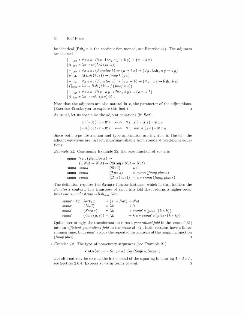
64 Ralf Hinze
be identical (Rshx x is the continuation monad, see Exercise 44). The adjunctsare defined
⌊−⌋Lsh ∶ ∀x a b . (∀y . Lshx a y → b y)→ (a → b x)⌊α⌋Lsh = λs → α (Lsh (id , s))⌈−⌉Lsh ∶ ∀x a b . (Functor b)⇒ (a → b x)→ (∀y . Lshx a y → b y)⌈g⌉Lsh = λ(Lsh (k , s))→ fmap k (g s)⌊−⌋Rsh ∶ ∀x a b . (Functor a)⇒ (a x → b)→ (∀y . a y → Rshx b y)⌊f ⌋Rsh = λs → Rsh (λk → f (fmap k s))⌈−⌉Rsh ∶ ∀x a b . (∀y . a y → Rshx b y)→ (a x → b)⌈β⌉Rsh = λs → rsh○ (β s) id .
Note that the adjuncts are also natural in x , the parameter of the adjunctions.(Exercise 45 asks you to explore this fact.) ⊓⊔As usual, let us specialise the adjoint equations (in Set).
x ⋅ (−X ) in = Ψ x ⇐⇒ ∀s . x (in X s) = Ψ x s
(−X )out ⋅ x = Ψ x ⇐⇒ ∀a . out X (x a) = Ψ x a
Since both type abstraction and type application are invisible in Haskell, theadjoint equations are, in fact, indistinguishable from standard fixed-point equa-tions.
Example 24. Continuing Example 22, the base function of suma is
suma ∶ ∀x . (Functor x)⇒(x Nat → Nat)→ (Array x Nat → Nat)
suma suma (Null) = 0suma suma (Zero s) = suma (fmap plus s)suma suma (One (a, s)) = a + suma (fmap plus s) .
The definition requires the Array x functor instance, which in turn induces theFunctor x context. The transpose of suma is a fold that returns a higher-orderfunction: suma ′ ∶ Array → RshNat Nat .
suma ′ ∶ ∀x . Array x → (x → Nat)→ Natsuma ′ (Null) = λk → 0suma ′ (Zero s) = λk → suma ′ s (plus ⋅ (k × k))suma ′ (One (a, s)) = λk → k a + suma ′ s (plus ⋅ (k × k)) .
Quite interestingly, the transformation turns a generalised fold in the sense of [31]into an efficient generalised fold in the sense of [32]. Both versions have a linearrunning time, but suma ′ avoids the repeated invocations of the mapping function(fmap plus). ⊓⊔
∗ Exercise 42. The type of non-empty sequences (see Example 21)
dataSequa = Single a ∣ Cat (Sequa,Sequa)
can alternatively be seen as the free monad of the squaring functor SqA = A×A,see Section 2.6.4. Express sums in terms of eval . ⊓⊔

Generic Programming with Adjunctions 65
∗ Exercise 43. The type
dataTreea = Branch (Treea,a,Treea)
generalises the type of bifurcations (Example 2), abstracting away from the typeof labels. Capture generate ∶ Nat → TreeNat as an adjoint unfold. The type Treecan also be seen as the cofree comonad of the squaring functor SqA = A×A (seeExercise 34). Express generate in terms of trace. ⊓⊔
∗ Exercise 44. The purpose of this exercise is to show that the functor M = RshX Xis a monad for each choice of X ∶ C . There are at least two approaches: via thespecification or via the implementation.
1. If we specialise the specification of RshX , the adjunction −X ⊣ RshX , to(setting B ∶=X )
⌊−⌋ ∶ C (AX ,X ) ≅ C C (A,M) ∶ ⌈−⌉ ,
we obtain an isomorphism natural in the functor A. This suggests to definethe unit and the multiplication of the monad by
return = ⌊id⌋ ,join = ⌊e ⋅M e⌋where e = ⌈id⌉ .
Note that the arrow e ∶ C (MX ,X ) runs a computation. Show that returnand join satisfy the monad laws (see Exercise 30).
2. If the monad is implemented by MA =∏C (A,X ) . X , then we can use thecombinators of Section 2.5.7 to define
return =i
k . k ,
join =i
k . ππk.
Show that return and join thus defined satisfy the monad laws. Try to re-late the definitions to the implementation of the continuation monad fromHaskell’s standard libraries. ⊓⊔
∗ Exercise 45. Like the curry adjunction, −X ⊣ RshX is an adjunction with aparameter. Apply Exercise 35 to show that there is a unique way to turn Rshinto a bifunctor, so that the bijection C (AX ,B) ≅ C D(A,RshX B) is also naturalin X :
C (A X ,B)⌊−⌋
≻ C D(A,RshX B)
C (A X ,B)
C (Ap,B)⋎
⌊−⌋≻ C D(A,RshX B) ,
C D(A,Rshp B)⋎
where p ∶ D(X , X ). Explore. ⊓⊔

66 Ralf Hinze
3.3.5 Type Composition. Continuing the theme of the last section, func-tions over parametric types, consider the following example.
Example 25. The function join defined
join ∶ ∀a . µSequ (Sequa) → Sequajoin (In (Single s)) = sjoin (In (Cat (l , r))) = In (Cat (join l , join r))
flattens a non-empty sequence of non-empty sequences. ⊓⊔
The definition has the structure of an ordinary fold, but again the type is notquite right: we need a natural transformation of type µSequ → G, but join hastype µSequ○Sequ→Sequ. Can we fit the definition into the framework of adjointequations? The answer is an emphatic “Yes, we Kan!” Similar to the developmentof the previous section, the first step is to identify a left adjoint. We alreadyknow that pre-composition is a functor (Section 2.2.3). Using this higher-orderfunctor we can assign join the type (−○Sequ) (µSequ) → Sequ. (We interpretSequ○Sequ as (−○Sequ)Sequ rather than (Sequ○−)Sequ because the outer list,written µSequ for emphasis, drives the recursion.)
As a second step, we have to construct the right adjoint of the higher-orderfunctor. It turns out that this is a well-studied problem in category theory.Similar to the situation of the previous section, under some conditions −○J hasboth a left and a right adjoint. For variety, we derive the latter.
F○J →G
≅ { natural transformation as an end [8, p.223] }∀Y ∶ C . E (F (JY ),GY )
≅ { Yoneda Lemma (85) }∀Y ∶ C . ∀X ∶ D . D(X , JY )→ E (FX ,GY )
≅ { power: I → C (Y ,B) ≅ C (Y ,∏ I . B) (52) }∀Y ∶ C . ∀X ∶ D . E (FX ,∏D(X , JY ) . GY )
≅ { interchange of quantifiers [8, p.231f] }∀X ∶ D . ∀Y ∶ C . E (FX ,∏D(X , JY ) . GY )
≅ { the hom-functor E (A,−) preserves ends [8, p.225] }∀X ∶ D . E (FX ,∀Y ∶ C .∏D(X , JY ) . GY )
≅ { define RanJG = λX ∶ D . ∀Y ∶ C .∏D(X , JY ) . GY }∀X ∶ D . E (FX ,RanJGX )
≅ { natural transformation as an end [8, p.223] }F → RanJG
Since each step is natural in F and G, the composite isomorphism is also naturalin F and G. The functor RanJG is called the right Kan extension of G along J.(If we view J ∶ C → D as an inclusion functor, then RanJG ∶ D → E extends

Generic Programming with Adjunctions 67
G ∶ C → E to the whole of D .) The universally quantified object in the definitionof RanJ is a so-called end, which corresponds to a polymorphic type in Haskell.An end is usually written with an integral sign; I prefer the universal quantifier,in particular, as it blends with the notation for natural transformations. Andindeed, natural transformations are an example of an end: DC (F,G) = ∀X ∶C . D(FX ,GX ). We refer the interested reader to [8] for further details.
Dually, the left adjoint of −○J is called the left Kan extension and is definedLanJ F = λX ∶ D . ∃Y ∶ C . ∑D(JY ,X ) . FY . The existentially quantifiedobject is a coend, which corresponds to an existential type in Haskell (hence thenotation). The following diagrams summarise the type information.
C
E ≺G
≺LanJ F
≺
F
D
J
⋎
E D ≺LanJ�−○J ≻ E C ≺
−○J�
RanJ≻ E D
C
D
J
⋎ F≻
RanJG≻ E
G
≻
Definition 26. Like Exp, the definition of the right Kan extension requires rank-2types (the data constructor Ran has a rank-2 type).
newtypeRanj g x = Ran {ran○ ∶ ∀a . (x → j a)→ g a }instance Functor (Ranj g)where
fmap f (Ran h) = Ran (λk → h (k ⋅ f ))
The type Ranj g can be seen as a generalised continuation type—often, but notalways, the type constructors j and g are identical (RanJ J is known as thecodensity monad, see Exercise 46). Morally, j and g are functors. However, theirmapping functions are not needed to define the Ranj g instance of Functor .Hence, we omit the (Functor j ,Functor g) context. The adjuncts are defined
⌊−⌋Ran ∶ ∀j f g . (Functor f )⇒ (∀x . f (j x)→ g x)→ (∀x . f x → Ranj g x)⌊α⌋Ran = λs → Ran (λk → α (fmap k s))⌈−⌉Ran ∶ ∀j f g . (∀x . f x → Ranj g x)→ (∀x . f (j x)→ g x)⌈β⌉Ran = λs → ran○ (β s) id .
Note that the adjuncts are also natural in j , the parameter of the adjunction.(Exercise 47 asks you to explore this fact.)
Turning to the definition of the left Kan extension we require another exten-sion of the Haskell 2010 type system: existential types.
dataLanj f x = ∀a . Lan (j a → x , f a)instance Functor (Lanj f )where
fmap f (Lan (k , s)) = Lan (f ⋅ k , s) .
The existential quantifier is written as a universal quantifier in front of thedata constructor Lan. Ideally, Lanj should be given by a newtype declaration,

68 Ralf Hinze
but newtype constructors must not have an existential context (in GHC). Forsimilar reasons, we cannot use a destructor, that is, a selector function lan○. Thetype Lanj f can be seen as a generalised abstract data type: f a is the internalstate and j a → x the observer function—again, the type constructors j and fare likely to be identical (LanJ J is known as the density comonad). The adjunctsare given by
⌊−⌋Lan ∶ ∀j f g . (∀x . Lanj f x → g x)→ (∀x . f x → g (j x))⌊α⌋Lan = λs → α (Lan (id , s))⌈−⌉Lan ∶ ∀j f g . (Functor g)⇒ (∀x . f x → g (j x))→ (∀x . Lanj f x → g x)⌈β⌉Lan = λ(Lan (k , s))→ fmap k (β s) .
The duality of the construction is somewhat obscured in Haskell. ⊓⊔
As usual, let us specialise the adjoint equations (in Set).
x ⋅ (−○J) in = Ψ x ⇐⇒ ∀A . ∀s . x A (in (JA) s) = Ψ x A s
(−○J)out ⋅ x = Ψ x ⇐⇒ ∀A . ∀a . out (JA) (x A a) = Ψ x A a
The usual caveat applies when reading the equations as Haskell definitions: astype application is invisible, the derived equation is indistinguishable from theoriginal one.
Example 27. Continuing Example 25, the base function of join is straightfor-ward, except perhaps for the types.
join ∶ ∀x . (∀a . x (Sequa)→ Sequa)→(∀a .Sequ x (Sequa)→ Sequa)
join join (Single s) = sjoin join (Cat (l , r)) = In (Cat (join l , join r))
The base function join is a second-order natural transformation. The transposeof join is quite revealing. First of all, its type is
join ′ ∶ Sequ → RanSequ Sequ ≅ ∀a . Sequa → ∀b . (a → Sequ b)→ Sequ b .
The type suggests that join ′ is the bind of the monad Sequ (Exercise 42) andthis is indeed the case!
join ′ ∶ ∀a b . µSequa → (a → Sequ b)→ Sequ bjoin ′ as = λk → join (fmap k as)
For clarity, we have inlined RanSequ Sequ. ⊓⊔
Kan extensions generalise the constructions of the previous section: If thecategory C is non-empty (C ≠ 0), then we have LshA B ≅ Lan(KA) (KB) andRshA B ≅ Ran(KA) (KB), where K is the constant functor. Here is the proof for

Generic Programming with Adjunctions 69
the right adjoint:
FA→ B
≅ { arrows as natural transformations: A→ B ≅ KA →KB if C ≠ 0 }K (FA) →KB
= { K (FA) = F○KA }F○KA →KB
≅ { (−○J) ⊣ RanJ }F → RanKA (KB) .
Since adjoints are unique up to isomorphism (Section 2.5.8), we conclude thatRanKA○K ≅ RshA.
∗ Exercise 46. Kan extensions generalise shifts. Likewise, the codensity monadgeneralises the continuation monad. This exercise is due to Mac Lane [8, Exer-cise X.7.3]; it is solved in the forthcoming paper [33].
1. Generalise the argument of Exercise 44 to show that M = RanJ J is a monadfor each choice of J ∶ C → D . The functor M is called the codensity monadof J. (Specifically, if we specialise the adjunction (−○J) ⊣ RanJ to (G ∶= J)
⌊−⌋ ∶ DC (F○J, J) ≅ DD(F,M) ∶ ⌈−⌉ ,
we obtain a bijection natural in the functor F ∶ D → D . Unit and multiplica-tion of the codensity monad are given by
return = ⌊id⌋ ,join = ⌊e ⋅M○e⌋where e = ⌈id⌉ ,
where the natural transformation e ∶ DC (M○J, J) runs a computation.)2. Show that if R ∶ C → D has a left adjoint, L ⊣ R, then the codensity monad
of R is the monad induced by the adjunction, (R○L, η,R○ε○L). ⊓⊔
∗ Exercise 47. The adjunction (−○J) ⊣ RanJ is yet another example of an adjunc-tion with a parameter. Apply Exercise 35 to show that there is a unique wayto turn Ran into a higher-order bifunctor, so that the bijection E C (F○J,G) ≅E D(F,RanJG) is also natural in J:
E C (F○J,G)⌊−⌋
≻ E D(F,RanJG)
E C (F○J,G)
E C (F○α,G)⋎
⌊−⌋≻ E D(F,RanJG) ,
E D(F,RanαG)⋎
where α ∶ DC (J, J). Remember that −○= is a bifunctor (Section 2.2.3). Conse-quently, −○α is a higher-order natural transformation. Explore. ⊓⊔

70 Ralf Hinze
3.3.6 Swapping Arguments. So far we have considered inductive and coin-ductive types only in isolation. The following example introduces two functionsthat combine an inductive with a coinductive type.
Example 28. Bifurcations and functions over the binary numbers are in one-to-one correspondence. The functions tabulate and lookup witness the isomorphism.
tabulate ∶ (Nat → Nat)→ Treetabulate f = Branch (tabulate (f ⋅O), f N , tabulate (f ⋅ I ))lookup ∶ Tree → (Nat → Nat)lookup (Branch (l , v , r)) (N ) = vlookup (Branch (l , v , r)) (O b) = lookup l blookup (Branch (l , v , r)) (I b) = lookup r b
The first isomorphism tabulates a given function, producing an infinite tree ofits values. Its inverse looks up a binary number at a given position. ⊓⊔
Tabulation is a standard unfold, but what about lookup? Its type involves expo-nentials: lookup ∶ C (Tree,NatµNat). However, the curry adjunction −×X ⊣ (−)Xis not applicable here, as the right adjoint fixes the source object. We need itscounterpart, the functor X (−) ∶ C op → C , which fixes the target object (Ex-ercise 22). Since this functor is contravariant, the type of lookup is actually
C op((Nat(−))op (µNat),Tree), which suggests that the arrow is an adjoint fold!If we specialise the adjoint equation to C = Set and L = X (−), we obtain
x ⋅ L in = Ψ x ⇐⇒ ∀s . ∀a . x a (in s) = Ψ x a s .
So x is simply a curried function that recurses over the second argument.We have not mentioned unfolds so far. The reason is perhaps surprising. In
this particular case, an adjoint unfold is the same as an adjoint fold! Considerthe type of an adjoint unfold: C (A,R (νF)). Since R = X (−) is contravariant,the final coalgebra in C op is the initial algebra in C . Since furthermore X (−) isself-adjoint, we obtain the type of an adjoint fold: C (A,L (µF)) = C op(L (µF),A).
Table 4 summarises the adjunctions considered in this section.
Exercise 48. Exercise 32 asked you to explore the adjunction Free ⊣ U, whereU ∶ Mon→ Set is the functor that forgets about the additional structure of Mon.Explore adjoint folds of type Free (µF)→ A. ⊓⊔
3.4 Program Verification
In this section we develop the calculational properties of adjoint folds—the readeris invited to dualise the results to adjoint unfolds. Sections 3.4.1 is concernedwith laws that support structured point-free reasoning. Section 3.4.2 then shiftsthe focus from point-free to pointwise style. It presents a unifying proof methodthat can be readily adapted to support effective pointwise calculations.

Generic Programming with Adjunctions 71
Table 4. Adjunctions and types of recursion.
adjunction initial fixed-point equation final fixed-point equation
L ⊣ Rx ⋅ L in = Ψ x Rout ⋅ x = Ψ x
x ′ ⋅ in = ⌊Ψ ⌈x ′⌉⌋ out ⋅ x ′ = ⌈Ψ ⌊x ′⌋⌉
Id ⊣ Idstandard fold standard unfoldstandard fold standard unfold
− ×X ⊣ (−)X
parametrised fold curried unfold
x ⋅ (in ×X ) = Ψ x outX ⋅ x = Ψ xfold to an exponential unfold from a product
(X (−))op⊣ X (−)
swapped curried foldX in
⋅ x = Ψ xfold to an exponential
(+) ⊣∆
recursion from a coproduct ofmutual value recursion
mutually recursive typesout ⋅ x1 = Ψ1 ⟨x1, x2⟩out ⋅ x2 = Ψ2 ⟨x1, x2⟩
mutual value recursion on single recursion from amutually recursive types coproduct domain
∆ ⊣ (×)
mutual value recursionrecursion to a product ofmutually recursive types
x1 ⋅ in = Ψ1 ⟨x1, x2⟩x2 ⋅ in = Ψ2 ⟨x1, x2⟩
single recursion to a mutual value recursion onproduct domain mutually recursive types
⟨−, 0⟩ ⊣ Outl —
single value recursion onmutually recursive types
out1 ⋅ x = Ψ x‘mutual’ value recursion on
mutually recursive types
Outl ⊣ ⟨−, 1⟩
single value recursion on
—mutually recursive types
x ⋅ in1 = Ψ x‘mutual’ value recursion on
mutually recursive types
LshX ⊣ (−X ) —monomorphic unfold
out X ⋅ x = Ψ xunfold from a left shift
(−X ) ⊣ RshX
monomorphic fold—x ⋅ in X = Ψ x
fold to a right shift
LanJ ⊣ (−○J) —polymorphic unfold
out○J ⋅ x = Ψ xunfold from a left Kan extension
(−○J) ⊣ RanJ
polymorphic fold—x ⋅ in○J = Ψ x
fold to a right Kan extension

72 Ralf Hinze
3.4.1 Uniqueness Property. Adjoint folds enjoy the usual plethora of prop-erties. The fact that an adjoint initial fixed-point equation has a unique solutioncan be captured by the following equivalence, the uniqueness property.
x = ((Ψ ))L ⇐⇒ x ⋅ L in = Ψ x (98)
The uniqueness property has two simple consequences. First, substituting theleft-hand side into the right-hand side gives the computation law.
((Ψ ))L ⋅ L in = Ψ ((Ψ ))L (99)
The law has a straightforward operational reading: an application of an adjointfold is replaced by the body of the fold.
Second, instantiating x to id , we obtain the reflection law.
((Ψ ))L = id ⇐⇒ Ψ id = L in (100)
As an application of these identities, let us generalise the banana-split law [9].In Section 2.6.6 we have stated the law in terms of standard folds. However, itcan be readily ported to adjoint folds. First we introduce the counterpart of theproduct of two algebras (see also Exercise 49):
(Φ⊗ Ψ) x = Φ (outl ⋅ x)△ Ψ (outr ⋅ x) . (101)
It is worth pointing out that the definition of ⊗ mentions neither the base func-tor F nor the adjoint functor L—in a sense, the base functions are hiding unnec-essary detail.
Exercise 49. We have seen in Section 3.1.1 that base functions of type C (−,A)→C (F−,A) and F-algebras are in one-to-one correspondence. Show that ⊗ corre-sponds to the product of algebras (for L = Id). ⊓⊔
The generalised banana-split law then states
((Φ))L △ ((Ψ ))L = ((Φ⊗ Ψ ))L . (102)
For the proof we appeal to the uniqueness property (98); the obligation is dis-charged as follows.
(((Φ))L △ ((Ψ ))L) ⋅ L in
= { fusion (12) }((Φ))L ⋅ L in △ ((Ψ ))L ⋅ L in
= { computation (99) }Φ((Φ))L △ Ψ ((Ψ ))L
= { computation (9)–(10) }Φ (outl ⋅ (((Φ))L △ ((Ψ ))L))△ Ψ (outr ⋅ (((Φ))L △ ((Ψ ))L))
= { definition of ⊗ (101) }(Φ⊗ Ψ) (((Φ))L △ ((Ψ ))L)

Generic Programming with Adjunctions 73
Exercise 50. Consider the following string of isomorphisms.
LA→ B1 ×B2
≅ (LA→ B1) × (LA→ B2)≅ (A→ RB1) × (A→ RB2)≅ A→ RB1 × RB2
≅ A→ R (B1 ×B2)≅ LA→ B1 ×B2
Justify each step. Why is the generalised banana-split law in a sense unsurpris-ing? ⊓⊔
The fusion law states a condition for fusing an arrow h ∶ C (A,B) with anadjoint fold ((Φ))L ∶ C (L (µF),A) to form another adjoint fold ((Ψ ))L ∶ C (L (µF),B).The condition can be easily calculated.
h ⋅ ((Φ))L = ((Ψ ))L⇐⇒ { uniqueness property (98) }
h ⋅ ((Φ))L ⋅ L in = Ψ (h ⋅ ((Φ))L)⇐⇒ { computation (99) }
h ⋅Φ((Φ))L = Ψ (h ⋅ ((Φ))L)⇐Ô { abstracting away from ((Φ))L }
∀f . h ⋅Φ f = Ψ (h ⋅ f )
Consequently,
h ⋅ ((Φ))L = ((Ψ ))L ⇐Ô ∀f . h ⋅Φ f = Ψ (h ⋅ f ) . (103)
As for generalised banana-split, the fusion condition h ⋅ Φ f = Ψ (h ⋅ f ) mentionsneither the base functor F nor the adjoint functor L, which makes the law easyto use.
Exercise 51. Let a and b be the algebras corresponding to the base functions Φand Ψ (for L = Id). Show that
h ⋅ a = b ⋅ Fh ⇐⇒ ∀f . h ⋅Φ f = Ψ (h ⋅ f ) .
In other words, the fusion condition requires h to be an F-algebra homomor-phism. ⊓⊔
Example 29. The function height determines the height of a stack.
height ∶ Stack → Natheight Empty = 0height (Push (n, s)) = 1 + height s

74 Ralf Hinze
Let us show that height is a monoid homomorphism from the stack monoidto the monoid of natural numbers with addition, height ∶ (Stack ,Empty ,◇) →(Nat ,0,+):
height Empty = 0 , (104)
height (x ◇ y) = height x + height y , (105)
or, written in a point-free style,
height ⋅ empty = zero , (106)
height ⋅ cat = plus ⋅ (height × height) . (107)
Here zero is the constant arrow that yields 0, empty is the constant arrow thatyields Empty , and, finally, cat and plus are ◇ and + written prefix. The firstcondition (106) is an immediate consequence of height ’s definition. Regardingthe second condition (107), there is no obvious zone of attack, as neither theleft- nor the right-hand side is an adjoint fold. Consequently, we proceed in twosteps: we first demonstrate that the left-hand side can be fused to an adjointfold, and then we show that the right-hand side satisfies the adjoint fixed-pointequation of this fold.
For the first step, we are seeking a base function height2 so that
height ⋅ ((cat))L = ((height2))L ,
where L = −×Stack . The base function cat is defined in Example 13. Fusion (103)immediately gives us
∀cat . height ⋅ cat cat = height2 (height ⋅ cat) , (108)
from which we can easily synthesise a definition of height2:Case Empty:
height2 (height ⋅ cat) (Empty, y)= { specification of height2 (108) }
height (cat cat (Empty, y))= { definition of cat (Example 13) }
height y .
Case Push (a, x):
height2 (height ⋅ cat) (Push (a, x), y)= { specification of height2 (108) }
height (cat cat (Push (a, x), y))= { definition of cat (Example 13) and In ⋅Push = Push }
height (Push (a, cat (x , y)))= { definition of height }
1 + (height ⋅ cat) (x , y) .

Generic Programming with Adjunctions 75
Abstracting away from height ⋅ cat , we obtain
height2 ∶ ∀x . (L x → Nat)→ (L (Stack x) → Nat)height2 height2 (Empty, y) = height yheight2 height2 (Push (a, x), y) = 1 + height2 (x , y) .
For the second step, we have to show
plus ⋅ (height × height) = ((height2))L .
Appealing to uniqueness (98), we are left with the proof obligation
plus ⋅ (height × height) ⋅ L in = height2 (plus ⋅ (height × height)) ,
which is straightforward to discharge. ⊓⊔
3.4.2 Unique Fixed-point Principle. Assume that you want to prove theequality of two arrows. In the fortunate case that one of the arrows takes theform of an adjoint fold, we can either appeal to the uniqueness property, orpreferably, invoke the fusion law. Unfortunately, more often than not neitherarrow is given explicitly as an adjoint fold, in which case none of the laws isdirectly applicable. Property (107) illustrates this observation: both sides of theequation involve adjoint folds, but they are not themselves adjoint folds.
The following proof method, the unique fixed-point principle, provides a wayout of this dilemma. The idea is to demonstrate f ⋅ L in = Θ f and Θ g = g ⋅ L in.If the equation x ⋅ L in = Θ x has a unique solution, then we may conclude thatf = g . The important point is that we discover the base function Θ on the flyduring the calculation. A proof in this style is laid out as follows.
f ⋅ L in
= { why? }Θ f
∝ { x ⋅ L in = Θ x has a unique solution }Θ g
= { why? }g ⋅ L in
The symbol ∝ is meant to suggest a link connecting the upper and the lowerpart. Overall, the proof establishes that f = g . An analogous approach can beused to prove the equality of two adjoint unfolds.
Example 30. Let us show height (x ◇y) = height x +height y (105) a second time,this time using the unique fixed-point principle. For reasons of brevity it is usefulto condense the definitions of cat and height into single equations (we abbreviate

76 Ralf Hinze
Empty and Push by E and P).
cat ∶ (µStack, µStack)→ µStackcat (In s, u) = case s of {E→ u;P (a, t)→ In (P (a, cat (t ,u)))}height ∶ µStack→ Natheight (In s) = case s of {E→ 0;P (a, t)→ 1 + height t }
Expressing the calculation in a pointwise style leads to a more attractive proof,which proceeds as follows:
height (cat (In s,u))= { definition of cat }
height (case s of {E→ u;P (a, t)→ In (P (a, cat (t ,u)))})= { case-fusion }
case s of {E→ height u;P (a, t)→ height (In (P (a, cat (t ,u))))}= { definition of height }
case s of {E→ height u;P (a, t)→ 1 + height (cat (t ,u))}∝ { x (In s,u) = case s of {E→ height u;P (a, t)→ 1 + x (t ,u)} }
case s of {E→ height u;P (a, t)→ 1 + (height t + height u)}= { (Nat ,0,+) is a monoid }
case s of {E→ 0 + height u;P (a, t)→ (1 + height t) + height u }= { case-fusion }
(case s of {E→ 0;P (a, t)→ 1 + height t }) + height u
= { definition of height }height (In s) + height u .
Note that height (cat (In s,u)) = height (In s) + height u is the pointwise versionof height ⋅ cat ⋅ L in = plus ⋅ (height × height) ⋅ L in. Likewise, case-fusion is thepointwise variant of join-fusion (21), k ⋅ (g1 ▽ g2) = k ⋅ g1 ▽ k ⋅ g2.
The proof is short and sweet—every step is more or less forced. Furthermore,the central step, the application of the monoidal laws, stands out clearly. Alongthe way we have re-discovered the function height2 . It also served as the link inthe original proof, which established height ⋅cat = height2 = plus ⋅(height×height)in two steps. The new proof format merges the two separate proofs into one. ⊓⊔
On the face of it the proof above is tantalisingly close to a conventional inductiveproof, with in marking the induction argument and ∝ marking the applicationof the induction hypothesis. Indeed, in the case of Set a unique fixed-pointproof can be easily converted into an inductive proof. (The converse is true ifthe inductive proof establishes the equality of two functions: ∀x . f x = g x .)However, the unique fixed-point principle is agnostic of the underlying categoryand furthermore it works equally well for coinductive types.

Generic Programming with Adjunctions 77
Exercise 52. Show that (Stack ,Empty ,◇) is a monoid:
Empty ◇ s = s = s ◇Empty ,
(s ◇ t) ◇ u = s ◇ (t ◇ u) ,
or, written in a point-free style,
cat ⋅ (empty △ id) = id = cat ⋅ (id △ empty) ,
cat ⋅ (cat × id) = cat ⋅ (id × cat) ⋅ assocr ,
where assocr ∶ (A ×B) ×C ≅ A × (B ×C ) is the standard isomorphism betweennested products. ⊓⊔
4 Further Reading
This section provides some background on our subject, including references forfurther reading. A more in-depth appreciation of related work can be found inthe article “Adjoint Folds and Unfolds—An Extended Study” [11].
Category theory. The categorical trinity—category, functor and natural trans-formation—was discovered by Eilenberg and Mac Lane. The first treatment ofcategories in their own right appeared in 1945 [34]—the paper investigates thenotion of a natural isomorphism and is well worth reading. The definitive refer-ence for category theory is Mac Lane’s masterpiece [8]. Introductory textbooksto category theory include Awodey [35], Barr and Wells [36] and Pierce [37].
The notion of an adjunction was introduced by Daniel Kan in 1958 [7]. Ry-deheard [38] illustrates the concept using the free construction of a monoid as arunning example, solving some of our exercises. (In the 1980s and 1990s therewas a series of conferences on “Category Theory and Computer Science”; thispaper appeared as a tutorial contribution to the first incarnation, which wascalled “Category Theory and Computer Programming”.) Spivey [39] exploredthe categorical background of Bird’s theory of lists [40, 41], later known as theBird-Meertens formalism. Our calculational treatment of adjunctions is inspiredby Fokkinga and Meertens’ paper [42].
Recursion schemes. There is a large body of work on recursion schemes or‘morphisms’. Utilising the categorical notions of functors and natural trans-formations, Malcolm [43] generalised the Bird-Meertens formalism to arbitrarydatatypes. His work assumed Set as the underlying category and was adaptedby Meijer et al. [5] to the category Cpo. The latter paper also popularisedthe now famous terms catamorphism and anamorphism (for folds and unfolds),along with the banana and lens brackets (((−)) and [(−)]). Fokkinga [44] capturedmutually recursive functions by mutumorphisms. An alternative solution to the‘append -problem’ was proposed by Pardo [45]: he introduces folds with parame-ters and uses them to implement generic accumulations. Building on the work

78 Ralf Hinze
of Hagino [46], Malcolm [43] and many others, Bird and de Moor gave a compre-hensive account of the “Algebra of Programming” in their seminal textbook [9].The textbook puts a particular emphasis on a relational approach to programconstruction—moving from the concept of a category to the richer structure ofan allegory.
The discovery of nested datatypes and their expressive power [24, 47, 48] ledto a flurry of research. Standard folds on nested datatypes, which are naturaltransformations by construction, were perceived as not being expressive enough.The paper “Generalised folds for nested datatypes” by Bird and Paterson [31]addressed the problem by adding extra parameters to folds leading to the notionof a generalised fold. The second part of these lecture notes is, in fact, based ontheir work. In order to show that generalised folds are uniquely defined, theydiscuss conditions to ensure that the more general equation x ⋅L in = Ψ x , our ad-joint initial fixed-point equation, uniquely defines x . Two solutions are providedto this problem, the second of which requires L to have a right adjoint. Theyalso show that the right Kan extension is the right adjoint of pre-composition.
An alternative, type-theoretic approach to (co)inductive types was proposedby Mendler [21]. His induction combinators Rµ and Sν map a base function to itsunique fixed point. Strong normalisation is guaranteed by the polymorphic typeof the base function. The first categorical justification of Mendler-style recursionwas given by De Bruin [49].
Other recursion schemes. We have shown that many recursion schemes fall underthe umbrella of adjoint (un)folds. However, we cannot reasonably expect that ad-joint (un)folds subsume all existing species of morphisms. For instance, a largelyorthogonal extension of standard folds are recursion schemes from comonads [50,51]. Very briefly, given a comonad N and a distributive law α ∶ F○N → N○F, wecan define an arrow f = ((N in ⋅ α)) ∶ µF → N (µF) that fans out a data structure.Then the equation in the unknown x ∶ µF→ A,
x ⋅ in = a ⋅ F (N x ⋅ f ) ,
has a unique solution for every algebra a ∶ F (NA) → A. This scheme includesso-called histomorphisms as a special case (the Fibonacci function is an exampleof a histomorphism).
We have noted that initial algebras and final coalgebras are different entities.The fact that µF and νF are not compatible in general has the unfortunate conse-quence that we cannot freely combine folds (consumers) and unfolds (producers).A way out of this dilemma is to use hylomorphisms based on recursive coalgebrasas a structured recursion scheme [52]. Very briefly, a coalgebra ⟨C , c⟩ is calledrecursive if for every algebra ⟨A, a⟩ the equation in the unknown x ∶ C (C ,A),
x = a ⋅G x ⋅ c , (109)
has a unique solution. The equation captures the divide-and-conquer patternof computation: a problem is divided into sub-problems (c), the sub-problemsare solved recursively (G x ), and finally the sub-solutions are combined into a

Generic Programming with Adjunctions 79
single solution (a). The uniquely defined arrow x is called a hylomorphism. Hy-lomorphisms are more expressive than adjoint folds. The added expressive powercomes at a price, however. Hylomorphisms sometimes suffer from the practicalproblem that a suitable control functor (G above) is hard to find, see [11] for amore in-depth comparison.
Type fusion. The initial algebra approach to the semantics of datatypes origi-nates in the work of Lambek [13] on fixed points in categories. Lambek suggeststhat lattice theory provides a fruitful source of inspiration for results in categorytheory. This viewpoint was taken up by Backhouse [53], who generalised a num-ber of lattice-theoretic fixed point rules to category theory. One important lawis type fusion, which allows us to fuse an application of a functor with an initialalgebra to form another initial algebra
L (µF) ≅ µG ⇐Ô L○F ≅ G○L .
The witnesses of the isomorphism L (µF) ≅ µG can be defined as solutions of(adjoint) fixed point equations. Using type fusion one can show, for instance,
µListNat ≅ µStack ,
which allows us to relate the functions total and sums. The paper [11] containsmany more examples and also shows the intimate link between adjoint (un)foldsand type fusion.
5 Conclusion
Adjunctions have proved to be one of the most important ideas in categorytheory, predominantly due to their ubiquity. Many mathematical constructionsturn out to be adjoint functors that form adjunctions, with Mac Lane [8, p.vii]famously saying, “Adjoint functors arise everywhere.”
The same is probably true of computing science. Every fundamental typeor type constructor—initial object, final object, sum, product, exponential, freealgebra, cofree coalgebra—arises out of an adjunction. An adjunction features anamazing economy of expression, combining introduction-, elimination, β- and η-rules in a single statement. Indeed, suitable categories of discourse can be definedjust using adjunctions, for example, a category is called cartesian closed if thefollowing adjunctions exist: ∆ ⊣ 1, ∆ ⊣ ×, and − × X ⊣ (−)X for each choiceof X .
Adjoint folds and unfolds strike a fine balance between expressiveness andease of use. We have shown that many Haskell functions fit under this banner.The mechanics are straightforward: given a (co)recursive function, we abstractaway from the recursive calls, additionally removing occurrences of in and outthat guard those calls. In Set termination and productivity are ensured by anaturality condition on the resulting base function. The categorical concept ofan adjunction plays a central role in this development. In a sense, each adjunc-tion captures a different recursion scheme—accumulating parameters, mutual

80 Ralf Hinze
recursion, polymorphic recursion on nested datatypes and so forth—and allowsthe scheme to be viewed as an instance of an adjoint (un)fold.
Acknowledgements. I am grateful to Nate Foster, Jeremy Gibbons, Jose PedroMagalhaes and Nicolas Wu for proof-reading several drafts of these lecture notes.They spotted numerous errors and suggested many improvements regarding styleand presentation.
References
1. Jones, M.P.: A system of constructor classes: overloading and implicit higher-orderpolymorphism. Journal of Functional Programming 5(1) (January 1995) 1–35
2. Wadler, P.: Theorems for free! In: The Fourth International Conference on Func-tional Programming Languages and Computer Architecture (FPCA’89), London,UK, Addison-Wesley Publishing Company (September 1989) 347–359
3. Wadler, P.: Comprehending monads. In: Proceedings of the 1990 ACM Conferenceon LISP and Functional Programming, Nice, ACM Press (June 1990) 61–78
4. McBride, C., Paterson, R.: Functional Pearl: Applicative programming with effects.Journal of Functional Programming 18(1) (2008) 1–13
5. Meijer, E., Fokkinga, M., Paterson, R.: Functional programming with bananas,lenses, envelopes and barbed wire. In Hughes, J., ed.: 5th ACM Conference onFunctional Programming Languages and Computer Architecture, FPCA’91, Cam-bridge, MA, USA. Volume 523 of Lecture Notes in Computer Science., SpringerBerlin / Heidelberg (1991) 124–144
6. Gibbons, J., Jones, G.: The under-appreciated unfold. In Felleisen, M., Hudak,P., Queinnec, C., eds.: Proceedings of the third ACM SIGPLAN internationalconference on Functional programming, ACM Press (1998) 273–279
7. Kan, D.M.: Adjoint functors. Transactions of the American Mathematical Society87(2) (1958) 294–329
8. Mac Lane, S.: Categories for the Working Mathematician. 2nd edn. GraduateTexts in Mathematics. Springer-Verlag, Berlin (1998)
9. Bird, R., De Moor, O.: Algebra of Programming. Prentice Hall Europe, London(1997)
10. Hinze, R.: A category theory primer (2010) www.cs.ox.ac.uk/ralf.hinze/
SSGIP10/Notes.pdf.11. Hinze, R.: Adjoint folds and unfolds—an extended study. Science of Computer
Programming (2011) to appear.12. Mulry, P.: Strong monads, algebras and fixed points. In Fourman, M., Johnstone,
P., Pitts, A., eds.: Applications of Categories in Computer Science. CambridgeUniversity Press (1992)
13. Lambek, J.: A fixpoint theorem for complete categories. Math. Zeitschr. 103(1968) 151–161
14. Hinze, R., James, D.W.H.: Reason isomorphically! In Oliveira, B.C., Zalewski, M.,eds.: Proceedings of the 6th ACM SIGPLAN workshop on Generic programming(WGP ’10), New York, NY, USA, ACM (September 2010) 85–96
15. Peyton Jones, S.: Haskell 98 Language and Libraries. Cambridge University Press(2003)
16. Cockett, R., Fukushima, T.: About Charity. Yellow Series Report 92/480/18,Dept. of Computer Science, Univ. of Calgary (June 1992)

Generic Programming with Adjunctions 81
17. The Coq Development Team: The Coq proof assistant reference manual (2010)http://coq.inria.fr.
18. Goguen, J.A., Thatcher, J.W., Wagner, E.G., Wright, J.B.: Initial algebra seman-tics and continuous algebras. Journal of the ACM 24(1) (January 1977) 68–95
19. Smyth, M.B., Plotkin, G.D.: The category-theoretic solution of recursive domainequations. SIAM Journal on Computing 11(4) (1982) 761–783
20. Sheard, T., Pasalic, T.: Two-level types and parameterized modules. Journal ofFunctional Programming 14(5) (September 2004) 547–587
21. Mendler, N.P.: Inductive types and type constraints in the second-order lambdacalculus. Annals of Pure and Applied Logic 51(1–2) (1991) 159–172
22. Gimenez, E.: Codifying guarded definitions with recursive schemes. In Dybjer, P.,Nordstrom, B., Smith, J.M., eds.: Types for Proofs and Programs, InternationalWorkshop TYPES’94, Bastad, Sweden, June 6-10, 1994, Selected Papers. Volume996 of Lecture Notes in Computer Science., Springer-Verlag (1995) 39–59
23. Okasaki, C.: Purely Functional Data Structures. Cambridge University Press(1998)
24. Bird, R., Meertens, L.: Nested datatypes. In Jeuring, J., ed.: Fourth Interna-tional Conference on Mathematics of Program Construction, MPC’98, Marstrand,Sweden. Volume 1422 of Lecture Notes in Computer Science., Springer Berlin /Heidelberg (June 1998) 52–67
25. Mycroft, A.: Polymorphic type schemes and recursive definitions. In Paul, M.,Robinet, B., eds.: Proceedings of the International Symposium on Programming,6th Colloquium, Toulouse, France. Volume 167 of Lecture Notes in Computer Sci-ence. (1984) 217–228
26. Hinze, R., Peyton Jones, S.: Derivable type classes. In Hutton, G., ed.: Proceed-ings of the 2000 ACM SIGPLAN Haskell Workshop. Volume 41(1) of ElectronicNotes in Theoretical Computer Science., Elsevier Science (August 2001) 5–35 Thepreliminary proceedings appeared as a University of Nottingham technical report.
27. Trifonov, V.: Simulating quantified class constraints. In: Haskell ’03: Proceedingsof the 2003 ACM SIGPLAN workshop on Haskell, New York, NY, USA, ACM(2003) 98–102
28. Lammel, R., Peyton Jones, S.: Scrap your boilerplate with class: extensible genericfunctions. In Pierce, B., ed.: Proceedings of the 2005 International Conference onFunctional Programming, Tallinn, Estonia, September 26–28, 2005. (September2005)
29. Meertens, L.: Paramorphisms. Formal Aspects of Computing 4 (1992) 413–42430. Backhouse, R., Bijsterveld, M., Van Geldrop, R., Van der Woude, J.: Category the-
ory as coherently constructive lattice theory (2003) Working Document, availablefrom http://www.cs.nott.ac.uk/~rcb/MPC/CatTheory.ps.gz.
31. Bird, R., Paterson, R.: Generalised folds for nested datatypes. Formal Aspects ofComputing 11(2) (1999) 200–222
32. Hinze, R.: Efficient generalized folds. In Jeuring, J., ed.: Proceedings of the secondWorkshop on Generic Programming. (2000) 1–16 The proceedings appeared as atechnical report of Universiteit Utrecht, UU-CS-2000-19.
33. Hinze, R.: Kan extensions for program optimisation—Or: art and dan explainan old trick. In Gibbons, J., Nogueira, P., eds.: 11th International Conference onMathematics of Program Construction (MPC ’12). Volume 7342 of Lecture Notesin Computer Science., Springer Berlin / Heidelberg (2012) 324–362
34. Eilenberg, S., MacLane, S.: General theory of natural equivalences. Transactionsof the American Mathematical Society 58(2) (September 1945) 231–294

82 Ralf Hinze
35. Awodey, S.: Category Theory. 2nd edn. Oxford University Press (2010)36. Barr, M., Wells, C.: Category Theory for Computing Science. 3rd edn. Les Pub-
lications CRM, Montreal (1999) The book is available from Centre de recherchesmathematiques http://crm.umontreal.ca/.
37. Pierce, B.C.: Basic Category Theory for Computer Scientists. The MIT Press(1991)
38. Rydeheard, D.: Adjunctions. In Pitt, D., Abramsky, S., Poigne, A., Rydeheard,D., eds.: Category Theory and Computer Science. Volume 240 of Lecture Notes inComputer Science., Springer Berlin / Heidelberg (1986) 51–57
39. Spivey, M.: A categorical approach to the theory of lists. In Van de Snepscheut,J., ed.: Mathematics of Program Construction. Volume 375 of Lecture Notes inComputer Science., Springer Berlin / Heidelberg (1989) 399–408
40. Bird, R.: An introduction to the theory of lists. In Broy, M., ed.: Proceedings of theNATO Advanced Study Institute on Logic of programming and calculi of discretedesign, Marktoberdorf, Germany, Springer Berlin / Heidelberg (1987) 5–42
41. Bird, R.: A calculus of functions for program derivation. Technical Report PRG-64,Programming Research Group, Oxford University Computing Laboratory (1987)
42. Fokkinga, M.M., Meertens, L.: Adjunctions. Technical Report Memoranda Inf94-31, University of Twente, Enschede, Netherlands (June 1994)
43. Malcolm, G.: Data structures and program transformation. Science of ComputerProgramming 14(2–3) (1990) 255–280
44. Fokkinga, M.M.: Law and Order in Algorithmics. PhD thesis, University of Twente(February 1992)
45. Pardo, A.: Generic accumulations. In Gibbons, J., Jeuring, J., eds.: Proceedingsof the IFIP TC2 Working Conference on Generic Programming, Schloss Dagstuhl.Volume 243., Kluwer Academic Publishers (July 2002) 49–78
46. Hagino, T.: A typed lambda calculus with categorical type constructors. In Pitt, D.,Poigne, A., Rydeheard, D., eds.: Category Theory and Computer Science. Volume283 of Lecture Notes in Computer Science. (1987)
47. Connelly, R.H., Morris, F.L.: A generalization of the trie data structure. Mathe-matical Structures in Computer Science 5(3) (September 1995) 381–418
48. Okasaki, C.: Catenable double-ended queues. In: Proceedings of the 1997 ACMSIGPLAN International Conference on Functional Programming, Amsterdam, TheNetherlands (June 1997) 66–74 ACM SIGPLAN Notices, 32(8), August 1997.
49. De Bruin, P.J.: Inductive types in constructive languages. PhD thesis, Universityof Groningen (1995)
50. Uustalu, T., Vene, V., Pardo, A.: Recursion schemes from comonads. Nordic J. ofComputing 8 (September 2001) 366–390
51. Bartels, F.: Generalised coinduction. Math. Struct. in Comp. Science 13 (2003)321—-348
52. Capretta, V., Uustalu, T., Vene, V.: Recursive coalgebras from comonads. Infor-mation and Computation 204(4) (2006) 437–468
53. Backhouse, R., Bijsterveld, M., Van Geldrop, R., Van der Woude, J.: Categoricalfixed point calculus. In Pitt, D., Rydeheard, D.E., Johnstone, P., eds.: Proceedingsof the 6th International Conference on Category Theory and Computer Science(CTCS ’95), Cambridge, UK. Volume 953 of Lecture Notes in Computer Science.,Springer-Verlag (August 1995) 159–179