genesys - users guide - keysightedadownload.software.keysight.com/.../pdf/users.pdf · no part of...
TRANSCRIPT


Genesys - Users Guide
1
Genesys 20102010
Users Guide

Genesys - Users Guide
2
© Agilent Technologies, Inc. 2000-20103501 Stevens Creek Blvd., Santa Clara, CA 95052 USANo part of this manual may be reproduced in any form or by any means (includingelectronic storage and retrieval or translation into a foreign language) without prioragreement and written consent from Agilent Technologies, Inc. as governed by UnitedStates and international copyright laws.
AcknowledgmentsMentor Graphics is a trademark of Mentor Graphics Corporation in the U.S. and othercountries. Microsoft®, Windows®, MS Windows®, Windows NT®, and MS-DOS® are U.S.registered trademarks of Microsoft Corporation. Pentium® is a U.S. registered trademarkof Intel Corporation. PostScript® and Acrobat® are trademarks of Adobe SystemsIncorporated. UNIX® is a registered trademark of the Open Group. Java™ is a U.S.trademark of Sun Microsystems, Inc. SystemC® is a registered trademark of OpenSystemC Initiative, Inc. in the United States and other countries and is used withpermission. MATLAB® is a U.S. registered trademark of The Math Works, Inc.. HiSIM2source code, and all copyrights, trade secrets or other intellectual property rights in and tothe source code in its entirety, is owned by Hiroshima University and STARC. DrawingInterchange file (DXF) is a trademark of Auto Desk, Inc. EMPOWER/ML, Genesys,SPECTRASYS, HARBEC, and TESTLINK are trademarks of Agilent Technologies, Inc. GDSIIis a trademark of Calma Company. Sonnet is a registered trademark of Sonnet Software,Inc.
Errata The ADS product may contain references to "HP" or "HPEESOF" such as in filenames and directory names. The business entity formerly known as "HP EEsof" is now partof Agilent Technologies and is known as "Agilent EEsof". To avoid broken functionality andto maintain backward compatibility for our customers, we did not change all the namesand labels that contain "HP" or "HPEESOF" references.
Warranty The material contained in this document is provided "as is", and is subject tobeing changed, without notice, in future editions. Further, to the maximum extentpermitted by applicable law, Agilent disclaims all warranties, either express or implied,with regard to this manual and any information contained herein, including but not limitedto the implied warranties of merchantability and fitness for a particular purpose. Agilentshall not be liable for errors or for incidental or consequential damages in connection withthe furnishing, use, or performance of this document or of any information containedherein. Should Agilent and the user have a separate written agreement with warrantyterms covering the material in this document that conflict with these terms, the warrantyterms in the separate agreement shall control.
Technology Licenses The hardware and/or software described in this document arefurnished under a license and may be used or copied only in accordance with the terms ofsuch license. Portions of this product include the SystemC software licensed under OpenSource terms, which are available for download at http://systemc.org/ . This software isredistributed by Agilent. The Contributors of the SystemC software provide this software"as is" and offer no warranty of any kind, express or implied, including without limitationwarranties or conditions or title and non-infringement, and implied warranties orconditions merchantability and fitness for a particular purpose. Contributors shall not beliable for any damages of any kind including without limitation direct, indirect, special,incidental and consequential damages, such as lost profits. Any provisions that differ fromthis disclaimer are offered by Agilent only.With respect to the portion of the Licensed Materials that describes the software andprovides instructions concerning its operation and related matters, "use" includes the rightto download and print such materials solely for the purpose described above.

Genesys - Users Guide
3
Restricted Rights Legend U.S. Government Restricted Rights. Software and technicaldata rights granted to the federal government include only those rights customarilyprovided to end user customers. Agilent provides this customary commercial license inSoftware and technical data pursuant to FAR 12.211 (Technical Data) and 12.212(Computer Software) and, for the Department of Defense, DFARS 252.227-7015(Technical Data - Commercial Items) and DFARS 227.7202-3 (Rights in CommercialComputer Software or Computer Software Documentation).

Genesys - Users Guide
4
The Genesys Environment . . . . . . . . . . . . . . . . . . . . . . . . . . . . . . . . . . . . . . . . . . . . . . . . . . 16 Contents . . . . . . . . . . . . . . . . . . . . . . . . . . . . . . . . . . . . . . . . . . . . . . . . . . . . . . . . . . . . 16 Starting Genesys . . . . . . . . . . . . . . . . . . . . . . . . . . . . . . . . . . . . . . . . . . . . . . . . . . . . . . . 16 Genesys Design Environment (User Interface) . . . . . . . . . . . . . . . . . . . . . . . . . . . . . . . . . . 18
Setting Global Options for Genesys . . . . . . . . . . . . . . . . . . . . . . . . . . . . . . . . . . . . . . . . . . . . 36 To set Global Options . . . . . . . . . . . . . . . . . . . . . . . . . . . . . . . . . . . . . . . . . . . . . . . . . . . . 36 General Options Tab . . . . . . . . . . . . . . . . . . . . . . . . . . . . . . . . . . . . . . . . . . . . . . . . . . . . 36 Startup Options Tab . . . . . . . . . . . . . . . . . . . . . . . . . . . . . . . . . . . . . . . . . . . . . . . . . . . . 37 Graph Options Tab . . . . . . . . . . . . . . . . . . . . . . . . . . . . . . . . . . . . . . . . . . . . . . . . . . . . . 38 Schematic Options Tab . . . . . . . . . . . . . . . . . . . . . . . . . . . . . . . . . . . . . . . . . . . . . . . . . . 39 Layout Options Tab . . . . . . . . . . . . . . . . . . . . . . . . . . . . . . . . . . . . . . . . . . . . . . . . . . . . . 40 Directories Options Tab . . . . . . . . . . . . . . . . . . . . . . . . . . . . . . . . . . . . . . . . . . . . . . . . . . 41 Language Options Tab . . . . . . . . . . . . . . . . . . . . . . . . . . . . . . . . . . . . . . . . . . . . . . . . . . . 41 Default Units Options Tab . . . . . . . . . . . . . . . . . . . . . . . . . . . . . . . . . . . . . . . . . . . . . . . . . 42 Appearance Options Tab . . . . . . . . . . . . . . . . . . . . . . . . . . . . . . . . . . . . . . . . . . . . . . . . . 43
Using Genesys . . . . . . . . . . . . . . . . . . . . . . . . . . . . . . . . . . . . . . . . . . . . . . . . . . . . . . . . . . 45 Contents . . . . . . . . . . . . . . . . . . . . . . . . . . . . . . . . . . . . . . . . . . . . . . . . . . . . . . . . . . . . 45
Analysis . . . . . . . . . . . . . . . . . . . . . . . . . . . . . . . . . . . . . . . . . . . . . . . . . . . . . . . . . . . . . . . 46 Annotations . . . . . . . . . . . . . . . . . . . . . . . . . . . . . . . . . . . . . . . . . . . . . . . . . . . . . . . . . . . . 47
Contents . . . . . . . . . . . . . . . . . . . . . . . . . . . . . . . . . . . . . . . . . . . . . . . . . . . . . . . . . . . . 47 Creating Annotations . . . . . . . . . . . . . . . . . . . . . . . . . . . . . . . . . . . . . . . . . . . . . . . . . . . . 47 Line Annotations . . . . . . . . . . . . . . . . . . . . . . . . . . . . . . . . . . . . . . . . . . . . . . . . . . . . . . . 48 Text Annotations . . . . . . . . . . . . . . . . . . . . . . . . . . . . . . . . . . . . . . . . . . . . . . . . . . . . . . . 48 Button Annotations (Widgets) . . . . . . . . . . . . . . . . . . . . . . . . . . . . . . . . . . . . . . . . . . . . . . 49 Slider Annotations (Widgets) . . . . . . . . . . . . . . . . . . . . . . . . . . . . . . . . . . . . . . . . . . . . . . 50 Variable Selector . . . . . . . . . . . . . . . . . . . . . . . . . . . . . . . . . . . . . . . . . . . . . . . . . . . . . . . 51
Designs . . . . . . . . . . . . . . . . . . . . . . . . . . . . . . . . . . . . . . . . . . . . . . . . . . . . . . . . . . . . . . . 53 Specific Types of Designs . . . . . . . . . . . . . . . . . . . . . . . . . . . . . . . . . . . . . . . . . . . . . . . . . 53 Contents . . . . . . . . . . . . . . . . . . . . . . . . . . . . . . . . . . . . . . . . . . . . . . . . . . . . . . . . . . . . 54 Design Properties . . . . . . . . . . . . . . . . . . . . . . . . . . . . . . . . . . . . . . . . . . . . . . . . . . . . . . 54 Modifying a Design . . . . . . . . . . . . . . . . . . . . . . . . . . . . . . . . . . . . . . . . . . . . . . . . . . . . . 54 Creating a Design . . . . . . . . . . . . . . . . . . . . . . . . . . . . . . . . . . . . . . . . . . . . . . . . . . . . . . 56 Using the Design Wizard . . . . . . . . . . . . . . . . . . . . . . . . . . . . . . . . . . . . . . . . . . . . . . . . . 56
Equations . . . . . . . . . . . . . . . . . . . . . . . . . . . . . . . . . . . . . . . . . . . . . . . . . . . . . . . . . . . . . 58 Contents . . . . . . . . . . . . . . . . . . . . . . . . . . . . . . . . . . . . . . . . . . . . . . . . . . . . . . . . . . . . 58 Using Engineering Language . . . . . . . . . . . . . . . . . . . . . . . . . . . . . . . . . . . . . . . . . . . . . . . 58 Using Math Language . . . . . . . . . . . . . . . . . . . . . . . . . . . . . . . . . . . . . . . . . . . . . . . . . . . . 58 Engineering Language Function Reference . . . . . . . . . . . . . . . . . . . . . . . . . . . . . . . . . . . . . 59 abs . . . . . . . . . . . . . . . . . . . . . . . . . . . . . . . . . . . . . . . . . . . . . . . . . . . . . . . . . . . . . . . . 64 abssum . . . . . . . . . . . . . . . . . . . . . . . . . . . . . . . . . . . . . . . . . . . . . . . . . . . . . . . . . . . . . 65 acos . . . . . . . . . . . . . . . . . . . . . . . . . . . . . . . . . . . . . . . . . . . . . . . . . . . . . . . . . . . . . . . . 65 acosh . . . . . . . . . . . . . . . . . . . . . . . . . . . . . . . . . . . . . . . . . . . . . . . . . . . . . . . . . . . . . . . 66 ang . . . . . . . . . . . . . . . . . . . . . . . . . . . . . . . . . . . . . . . . . . . . . . . . . . . . . . . . . . . . . . . . 66 ang360 . . . . . . . . . . . . . . . . . . . . . . . . . . . . . . . . . . . . . . . . . . . . . . . . . . . . . . . . . . . . . 66 array . . . . . . . . . . . . . . . . . . . . . . . . . . . . . . . . . . . . . . . . . . . . . . . . . . . . . . . . . . . . . . . 67 asin . . . . . . . . . . . . . . . . . . . . . . . . . . . . . . . . . . . . . . . . . . . . . . . . . . . . . . . . . . . . . . . . 67 asinh . . . . . . . . . . . . . . . . . . . . . . . . . . . . . . . . . . . . . . . . . . . . . . . . . . . . . . . . . . . . . . . 68 atan . . . . . . . . . . . . . . . . . . . . . . . . . . . . . . . . . . . . . . . . . . . . . . . . . . . . . . . . . . . . . . . . 68 atanh . . . . . . . . . . . . . . . . . . . . . . . . . . . . . . . . . . . . . . . . . . . . . . . . . . . . . . . . . . . . . . . 69 beta . . . . . . . . . . . . . . . . . . . . . . . . . . . . . . . . . . . . . . . . . . . . . . . . . . . . . . . . . . . . . . . . 69 betacdf . . . . . . . . . . . . . . . . . . . . . . . . . . . . . . . . . . . . . . . . . . . . . . . . . . . . . . . . . . . . . 69 betainc . . . . . . . . . . . . . . . . . . . . . . . . . . . . . . . . . . . . . . . . . . . . . . . . . . . . . . . . . . . . . . 70 betainv . . . . . . . . . . . . . . . . . . . . . . . . . . . . . . . . . . . . . . . . . . . . . . . . . . . . . . . . . . . . . 70 betaln . . . . . . . . . . . . . . . . . . . . . . . . . . . . . . . . . . . . . . . . . . . . . . . . . . . . . . . . . . . . . . 71 betapdf . . . . . . . . . . . . . . . . . . . . . . . . . . . . . . . . . . . . . . . . . . . . . . . . . . . . . . . . . . . . . 71

Genesys - Users Guide
5
ceil . . . . . . . . . . . . . . . . . . . . . . . . . . . . . . . . . . . . . . . . . . . . . . . . . . . . . . . . . . . . . . . . 72 column . . . . . . . . . . . . . . . . . . . . . . . . . . . . . . . . . . . . . . . . . . . . . . . . . . . . . . . . . . . . . . 72 complex . . . . . . . . . . . . . . . . . . . . . . . . . . . . . . . . . . . . . . . . . . . . . . . . . . . . . . . . . . . . . 73 concatcolumns . . . . . . . . . . . . . . . . . . . . . . . . . . . . . . . . . . . . . . . . . . . . . . . . . . . . . . . . 73 conj . . . . . . . . . . . . . . . . . . . . . . . . . . . . . . . . . . . . . . . . . . . . . . . . . . . . . . . . . . . . . . . . 73 cos . . . . . . . . . . . . . . . . . . . . . . . . . . . . . . . . . . . . . . . . . . . . . . . . . . . . . . . . . . . . . . . . 74 cosh . . . . . . . . . . . . . . . . . . . . . . . . . . . . . . . . . . . . . . . . . . . . . . . . . . . . . . . . . . . . . . . 74 Cp . . . . . . . . . . . . . . . . . . . . . . . . . . . . . . . . . . . . . . . . . . . . . . . . . . . . . . . . . . . . . . . . . 75 Cpk . . . . . . . . . . . . . . . . . . . . . . . . . . . . . . . . . . . . . . . . . . . . . . . . . . . . . . . . . . . . . . . . 75 CpkLower . . . . . . . . . . . . . . . . . . . . . . . . . . . . . . . . . . . . . . . . . . . . . . . . . . . . . . . . . . . . 76 CpkUpper . . . . . . . . . . . . . . . . . . . . . . . . . . . . . . . . . . . . . . . . . . . . . . . . . . . . . . . . . . . . 76 db . . . . . . . . . . . . . . . . . . . . . . . . . . . . . . . . . . . . . . . . . . . . . . . . . . . . . . . . . . . . . . . . . 77 db10 . . . . . . . . . . . . . . . . . . . . . . . . . . . . . . . . . . . . . . . . . . . . . . . . . . . . . . . . . . . . . . . 77 dbm . . . . . . . . . . . . . . . . . . . . . . . . . . . . . . . . . . . . . . . . . . . . . . . . . . . . . . . . . . . . . . . . 78 dbmtow . . . . . . . . . . . . . . . . . . . . . . . . . . . . . . . . . . . . . . . . . . . . . . . . . . . . . . . . . . . . . 78 dbpolar . . . . . . . . . . . . . . . . . . . . . . . . . . . . . . . . . . . . . . . . . . . . . . . . . . . . . . . . . . . . . 78 derivative . . . . . . . . . . . . . . . . . . . . . . . . . . . . . . . . . . . . . . . . . . . . . . . . . . . . . . . . . . . . 79 dev_lin_phase . . . . . . . . . . . . . . . . . . . . . . . . . . . . . . . . . . . . . . . . . . . . . . . . . . . . . . . . . 79 diag . . . . . . . . . . . . . . . . . . . . . . . . . . . . . . . . . . . . . . . . . . . . . . . . . . . . . . . . . . . . . . . . 79 iftrue . . . . . . . . . . . . . . . . . . . . . . . . . . . . . . . . . . . . . . . . . . . . . . . . . . . . . . . . . . . . . . . 80 unwrap . . . . . . . . . . . . . . . . . . . . . . . . . . . . . . . . . . . . . . . . . . . . . . . . . . . . . . . . . . . . . 80 erf . . . . . . . . . . . . . . . . . . . . . . . . . . . . . . . . . . . . . . . . . . . . . . . . . . . . . . . . . . . . . . . . . 80 erfc . . . . . . . . . . . . . . . . . . . . . . . . . . . . . . . . . . . . . . . . . . . . . . . . . . . . . . . . . . . . . . . . 81 exp . . . . . . . . . . . . . . . . . . . . . . . . . . . . . . . . . . . . . . . . . . . . . . . . . . . . . . . . . . . . . . . . 81 eye . . . . . . . . . . . . . . . . . . . . . . . . . . . . . . . . . . . . . . . . . . . . . . . . . . . . . . . . . . . . . . . . 82 fft . . . . . . . . . . . . . . . . . . . . . . . . . . . . . . . . . . . . . . . . . . . . . . . . . . . . . . . . . . . . . . . . . 82 floor . . . . . . . . . . . . . . . . . . . . . . . . . . . . . . . . . . . . . . . . . . . . . . . . . . . . . . . . . . . . . . . 83 gamma . . . . . . . . . . . . . . . . . . . . . . . . . . . . . . . . . . . . . . . . . . . . . . . . . . . . . . . . . . . . . 84 gammainc . . . . . . . . . . . . . . . . . . . . . . . . . . . . . . . . . . . . . . . . . . . . . . . . . . . . . . . . . . . 84 gammaln . . . . . . . . . . . . . . . . . . . . . . . . . . . . . . . . . . . . . . . . . . . . . . . . . . . . . . . . . . . . 84 gammatoz . . . . . . . . . . . . . . . . . . . . . . . . . . . . . . . . . . . . . . . . . . . . . . . . . . . . . . . . . . . 85 getdbunit . . . . . . . . . . . . . . . . . . . . . . . . . . . . . . . . . . . . . . . . . . . . . . . . . . . . . . . . . . . . 85 getindep . . . . . . . . . . . . . . . . . . . . . . . . . . . . . . . . . . . . . . . . . . . . . . . . . . . . . . . . . . . . . 86 getindepvalue . . . . . . . . . . . . . . . . . . . . . . . . . . . . . . . . . . . . . . . . . . . . . . . . . . . . . . . . . 86 getunits . . . . . . . . . . . . . . . . . . . . . . . . . . . . . . . . . . . . . . . . . . . . . . . . . . . . . . . . . . . . . 87 hb_gain . . . . . . . . . . . . . . . . . . . . . . . . . . . . . . . . . . . . . . . . . . . . . . . . . . . . . . . . . . . . . 87 hb_getspcomp . . . . . . . . . . . . . . . . . . . . . . . . . . . . . . . . . . . . . . . . . . . . . . . . . . . . . . . . 88 hb_getspcompdbm . . . . . . . . . . . . . . . . . . . . . . . . . . . . . . . . . . . . . . . . . . . . . . . . . . . . . 89 hb_iipn . . . . . . . . . . . . . . . . . . . . . . . . . . . . . . . . . . . . . . . . . . . . . . . . . . . . . . . . . . . . . 90 hb_ipn . . . . . . . . . . . . . . . . . . . . . . . . . . . . . . . . . . . . . . . . . . . . . . . . . . . . . . . . . . . . . . 91 hb_LargeS . . . . . . . . . . . . . . . . . . . . . . . . . . . . . . . . . . . . . . . . . . . . . . . . . . . . . . . . . . . 92 hb_LargeSmix . . . . . . . . . . . . . . . . . . . . . . . . . . . . . . . . . . . . . . . . . . . . . . . . . . . . . . . . . 93 hb_oipn . . . . . . . . . . . . . . . . . . . . . . . . . . . . . . . . . . . . . . . . . . . . . . . . . . . . . . . . . . . . . 94 hb_spurious . . . . . . . . . . . . . . . . . . . . . . . . . . . . . . . . . . . . . . . . . . . . . . . . . . . . . . . . . . 95 hb_totalsp . . . . . . . . . . . . . . . . . . . . . . . . . . . . . . . . . . . . . . . . . . . . . . . . . . . . . . . . . . . 96 hb_transgain . . . . . . . . . . . . . . . . . . . . . . . . . . . . . . . . . . . . . . . . . . . . . . . . . . . . . . . . . 97 hb_transgaindb . . . . . . . . . . . . . . . . . . . . . . . . . . . . . . . . . . . . . . . . . . . . . . . . . . . . . . . . 98 hermitian . . . . . . . . . . . . . . . . . . . . . . . . . . . . . . . . . . . . . . . . . . . . . . . . . . . . . . . . . . . . 98 histogram . . . . . . . . . . . . . . . . . . . . . . . . . . . . . . . . . . . . . . . . . . . . . . . . . . . . . . . . . . . . 99 identity . . . . . . . . . . . . . . . . . . . . . . . . . . . . . . . . . . . . . . . . . . . . . . . . . . . . . . . . . . . . . 99 iff . . . . . . . . . . . . . . . . . . . . . . . . . . . . . . . . . . . . . . . . . . . . . . . . . . . . . . . . . . . . . . . . . 100 ifft . . . . . . . . . . . . . . . . . . . . . . . . . . . . . . . . . . . . . . . . . . . . . . . . . . . . . . . . . . . . . . . . . 100 im . . . . . . . . . . . . . . . . . . . . . . . . . . . . . . . . . . . . . . . . . . . . . . . . . . . . . . . . . . . . . . . . . 101 imag . . . . . . . . . . . . . . . . . . . . . . . . . . . . . . . . . . . . . . . . . . . . . . . . . . . . . . . . . . . . . . . 101 integrate . . . . . . . . . . . . . . . . . . . . . . . . . . . . . . . . . . . . . . . . . . . . . . . . . . . . . . . . . . . . 101

Genesys - Users Guide
6
interpolate . . . . . . . . . . . . . . . . . . . . . . . . . . . . . . . . . . . . . . . . . . . . . . . . . . . . . . . . . . . 102 intersect . . . . . . . . . . . . . . . . . . . . . . . . . . . . . . . . . . . . . . . . . . . . . . . . . . . . . . . . . . . . . 103 inverse . . . . . . . . . . . . . . . . . . . . . . . . . . . . . . . . . . . . . . . . . . . . . . . . . . . . . . . . . . . . . . 104 kurtosis . . . . . . . . . . . . . . . . . . . . . . . . . . . . . . . . . . . . . . . . . . . . . . . . . . . . . . . . . . . . . 104 largeS . . . . . . . . . . . . . . . . . . . . . . . . . . . . . . . . . . . . . . . . . . . . . . . . . . . . . . . . . . . . . . 105 largeSconv . . . . . . . . . . . . . . . . . . . . . . . . . . . . . . . . . . . . . . . . . . . . . . . . . . . . . . . . . . . 106 largeSmix . . . . . . . . . . . . . . . . . . . . . . . . . . . . . . . . . . . . . . . . . . . . . . . . . . . . . . . . . . . . 107 lininterp . . . . . . . . . . . . . . . . . . . . . . . . . . . . . . . . . . . . . . . . . . . . . . . . . . . . . . . . . . . . . 109 ln . . . . . . . . . . . . . . . . . . . . . . . . . . . . . . . . . . . . . . . . . . . . . . . . . . . . . . . . . . . . . . . . . 109 log . . . . . . . . . . . . . . . . . . . . . . . . . . . . . . . . . . . . . . . . . . . . . . . . . . . . . . . . . . . . . . . . . 110 mag . . . . . . . . . . . . . . . . . . . . . . . . . . . . . . . . . . . . . . . . . . . . . . . . . . . . . . . . . . . . . . . . 110 matrix . . . . . . . . . . . . . . . . . . . . . . . . . . . . . . . . . . . . . . . . . . . . . . . . . . . . . . . . . . . . . . 111 max . . . . . . . . . . . . . . . . . . . . . . . . . . . . . . . . . . . . . . . . . . . . . . . . . . . . . . . . . . . . . . . . 111 mean . . . . . . . . . . . . . . . . . . . . . . . . . . . . . . . . . . . . . . . . . . . . . . . . . . . . . . . . . . . . . . . 111 median . . . . . . . . . . . . . . . . . . . . . . . . . . . . . . . . . . . . . . . . . . . . . . . . . . . . . . . . . . . . . 112 min . . . . . . . . . . . . . . . . . . . . . . . . . . . . . . . . . . . . . . . . . . . . . . . . . . . . . . . . . . . . . . . . 112 mode . . . . . . . . . . . . . . . . . . . . . . . . . . . . . . . . . . . . . . . . . . . . . . . . . . . . . . . . . . . . . . . 113 moment . . . . . . . . . . . . . . . . . . . . . . . . . . . . . . . . . . . . . . . . . . . . . . . . . . . . . . . . . . . . . 113 ndim . . . . . . . . . . . . . . . . . . . . . . . . . . . . . . . . . . . . . . . . . . . . . . . . . . . . . . . . . . . . . . . 114 NFtoVNI( NF, Rs, TempC ) . . . . . . . . . . . . . . . . . . . . . . . . . . . . . . . . . . . . . . . . . . . . . . . . 114 norm . . . . . . . . . . . . . . . . . . . . . . . . . . . . . . . . . . . . . . . . . . . . . . . . . . . . . . . . . . . . . . . 115 normcdf . . . . . . . . . . . . . . . . . . . . . . . . . . . . . . . . . . . . . . . . . . . . . . . . . . . . . . . . . . . . . 115 norminv . . . . . . . . . . . . . . . . . . . . . . . . . . . . . . . . . . . . . . . . . . . . . . . . . . . . . . . . . . . . . 116 normpdf . . . . . . . . . . . . . . . . . . . . . . . . . . . . . . . . . . . . . . . . . . . . . . . . . . . . . . . . . . . . . 116 numcols . . . . . . . . . . . . . . . . . . . . . . . . . . . . . . . . . . . . . . . . . . . . . . . . . . . . . . . . . . . . . 116 numrows . . . . . . . . . . . . . . . . . . . . . . . . . . . . . . . . . . . . . . . . . . . . . . . . . . . . . . . . . . . . 117 ones . . . . . . . . . . . . . . . . . . . . . . . . . . . . . . . . . . . . . . . . . . . . . . . . . . . . . . . . . . . . . . . 117 PortVolts . . . . . . . . . . . . . . . . . . . . . . . . . . . . . . . . . . . . . . . . . . . . . . . . . . . . . . . . . . . . 118 posterror . . . . . . . . . . . . . . . . . . . . . . . . . . . . . . . . . . . . . . . . . . . . . . . . . . . . . . . . . . . . 118 postwarning . . . . . . . . . . . . . . . . . . . . . . . . . . . . . . . . . . . . . . . . . . . . . . . . . . . . . . . . . . 119 pow . . . . . . . . . . . . . . . . . . . . . . . . . . . . . . . . . . . . . . . . . . . . . . . . . . . . . . . . . . . . . . . . 119 prctile . . . . . . . . . . . . . . . . . . . . . . . . . . . . . . . . . . . . . . . . . . . . . . . . . . . . . . . . . . . . . . 119 prod . . . . . . . . . . . . . . . . . . . . . . . . . . . . . . . . . . . . . . . . . . . . . . . . . . . . . . . . . . . . . . . 120 quantile . . . . . . . . . . . . . . . . . . . . . . . . . . . . . . . . . . . . . . . . . . . . . . . . . . . . . . . . . . . . . 121 rand . . . . . . . . . . . . . . . . . . . . . . . . . . . . . . . . . . . . . . . . . . . . . . . . . . . . . . . . . . . . . . . 121 randn . . . . . . . . . . . . . . . . . . . . . . . . . . . . . . . . . . . . . . . . . . . . . . . . . . . . . . . . . . . . . . . 122 re . . . . . . . . . . . . . . . . . . . . . . . . . . . . . . . . . . . . . . . . . . . . . . . . . . . . . . . . . . . . . . . . . 122 real . . . . . . . . . . . . . . . . . . . . . . . . . . . . . . . . . . . . . . . . . . . . . . . . . . . . . . . . . . . . . . . . 123 reshape . . . . . . . . . . . . . . . . . . . . . . . . . . . . . . . . . . . . . . . . . . . . . . . . . . . . . . . . . . . . . 123 resize . . . . . . . . . . . . . . . . . . . . . . . . . . . . . . . . . . . . . . . . . . . . . . . . . . . . . . . . . . . . . . . 124 reverse . . . . . . . . . . . . . . . . . . . . . . . . . . . . . . . . . . . . . . . . . . . . . . . . . . . . . . . . . . . . . 124 rltogamma . . . . . . . . . . . . . . . . . . . . . . . . . . . . . . . . . . . . . . . . . . . . . . . . . . . . . . . . . . . 125 rltoz . . . . . . . . . . . . . . . . . . . . . . . . . . . . . . . . . . . . . . . . . . . . . . . . . . . . . . . . . . . . . . . . 125 rotate . . . . . . . . . . . . . . . . . . . . . . . . . . . . . . . . . . . . . . . . . . . . . . . . . . . . . . . . . . . . . . 126 RsCondToThick . . . . . . . . . . . . . . . . . . . . . . . . . . . . . . . . . . . . . . . . . . . . . . . . . . . . . . . . 126 RsResToThick . . . . . . . . . . . . . . . . . . . . . . . . . . . . . . . . . . . . . . . . . . . . . . . . . . . . . . . . . 127 RsRhoToThick . . . . . . . . . . . . . . . . . . . . . . . . . . . . . . . . . . . . . . . . . . . . . . . . . . . . . . . . . 128
runanalysis . . . . . . . . . . . . . . . . . . . . . . . . . . . . . . . . . . . . . . . . . . . . . . . . . . . . . . . . . . . . 130 setindep . . . . . . . . . . . . . . . . . . . . . . . . . . . . . . . . . . . . . . . . . . . . . . . . . . . . . . . . . . . . . 130 setplottype . . . . . . . . . . . . . . . . . . . . . . . . . . . . . . . . . . . . . . . . . . . . . . . . . . . . . . . . . . . 130 setunits . . . . . . . . . . . . . . . . . . . . . . . . . . . . . . . . . . . . . . . . . . . . . . . . . . . . . . . . . . . . . 131 shape . . . . . . . . . . . . . . . . . . . . . . . . . . . . . . . . . . . . . . . . . . . . . . . . . . . . . . . . . . . . . . . 131 sin . . . . . . . . . . . . . . . . . . . . . . . . . . . . . . . . . . . . . . . . . . . . . . . . . . . . . . . . . . . . . . . . . 132 sinc . . . . . . . . . . . . . . . . . . . . . . . . . . . . . . . . . . . . . . . . . . . . . . . . . . . . . . . . . . . . . . . . 132 sinh . . . . . . . . . . . . . . . . . . . . . . . . . . . . . . . . . . . . . . . . . . . . . . . . . . . . . . . . . . . . . . . . 133

Genesys - Users Guide
7
size . . . . . . . . . . . . . . . . . . . . . . . . . . . . . . . . . . . . . . . . . . . . . . . . . . . . . . . . . . . . . . . . 133 skewness . . . . . . . . . . . . . . . . . . . . . . . . . . . . . . . . . . . . . . . . . . . . . . . . . . . . . . . . . . . . 134 sort . . . . . . . . . . . . . . . . . . . . . . . . . . . . . . . . . . . . . . . . . . . . . . . . . . . . . . . . . . . . . . . . 134 sqr . . . . . . . . . . . . . . . . . . . . . . . . . . . . . . . . . . . . . . . . . . . . . . . . . . . . . . . . . . . . . . . . 135 sqrt . . . . . . . . . . . . . . . . . . . . . . . . . . . . . . . . . . . . . . . . . . . . . . . . . . . . . . . . . . . . . . . . 135 std . . . . . . . . . . . . . . . . . . . . . . . . . . . . . . . . . . . . . . . . . . . . . . . . . . . . . . . . . . . . . . . . . 136 stos . . . . . . . . . . . . . . . . . . . . . . . . . . . . . . . . . . . . . . . . . . . . . . . . . . . . . . . . . . . . . . . . 136 stoy . . . . . . . . . . . . . . . . . . . . . . . . . . . . . . . . . . . . . . . . . . . . . . . . . . . . . . . . . . . . . . . . 137 stoz . . . . . . . . . . . . . . . . . . . . . . . . . . . . . . . . . . . . . . . . . . . . . . . . . . . . . . . . . . . . . . . . 137 substrateer . . . . . . . . . . . . . . . . . . . . . . . . . . . . . . . . . . . . . . . . . . . . . . . . . . . . . . . . . . . 137 substrateh . . . . . . . . . . . . . . . . . . . . . . . . . . . . . . . . . . . . . . . . . . . . . . . . . . . . . . . . . . . 137 substraterho . . . . . . . . . . . . . . . . . . . . . . . . . . . . . . . . . . . . . . . . . . . . . . . . . . . . . . . . . . 138 substraterough . . . . . . . . . . . . . . . . . . . . . . . . . . . . . . . . . . . . . . . . . . . . . . . . . . . . . . . . 138 substratetand . . . . . . . . . . . . . . . . . . . . . . . . . . . . . . . . . . . . . . . . . . . . . . . . . . . . . . . . . 138 substratemet . . . . . . . . . . . . . . . . . . . . . . . . . . . . . . . . . . . . . . . . . . . . . . . . . . . . . . . . . 139 sum . . . . . . . . . . . . . . . . . . . . . . . . . . . . . . . . . . . . . . . . . . . . . . . . . . . . . . . . . . . . . . . . 139 tan . . . . . . . . . . . . . . . . . . . . . . . . . . . . . . . . . . . . . . . . . . . . . . . . . . . . . . . . . . . . . . . . 140 tanh . . . . . . . . . . . . . . . . . . . . . . . . . . . . . . . . . . . . . . . . . . . . . . . . . . . . . . . . . . . . . . . . 140 tcdf . . . . . . . . . . . . . . . . . . . . . . . . . . . . . . . . . . . . . . . . . . . . . . . . . . . . . . . . . . . . . . . . 141 time . . . . . . . . . . . . . . . . . . . . . . . . . . . . . . . . . . . . . . . . . . . . . . . . . . . . . . . . . . . . . . . . 141 times . . . . . . . . . . . . . . . . . . . . . . . . . . . . . . . . . . . . . . . . . . . . . . . . . . . . . . . . . . . . . . . 142 timevector . . . . . . . . . . . . . . . . . . . . . . . . . . . . . . . . . . . . . . . . . . . . . . . . . . . . . . . . . . . 142 tinv . . . . . . . . . . . . . . . . . . . . . . . . . . . . . . . . . . . . . . . . . . . . . . . . . . . . . . . . . . . . . . . . 143 tpdf . . . . . . . . . . . . . . . . . . . . . . . . . . . . . . . . . . . . . . . . . . . . . . . . . . . . . . . . . . . . . . . . 143 transpose . . . . . . . . . . . . . . . . . . . . . . . . . . . . . . . . . . . . . . . . . . . . . . . . . . . . . . . . . . . . 144 union . . . . . . . . . . . . . . . . . . . . . . . . . . . . . . . . . . . . . . . . . . . . . . . . . . . . . . . . . . . . . . . 144 unwrap . . . . . . . . . . . . . . . . . . . . . . . . . . . . . . . . . . . . . . . . . . . . . . . . . . . . . . . . . . . . . 144 using . . . . . . . . . . . . . . . . . . . . . . . . . . . . . . . . . . . . . . . . . . . . . . . . . . . . . . . . . . . . . . . 145 var . . . . . . . . . . . . . . . . . . . . . . . . . . . . . . . . . . . . . . . . . . . . . . . . . . . . . . . . . . . . . . . . 145 vector . . . . . . . . . . . . . . . . . . . . . . . . . . . . . . . . . . . . . . . . . . . . . . . . . . . . . . . . . . . . . . 146 zeros . . . . . . . . . . . . . . . . . . . . . . . . . . . . . . . . . . . . . . . . . . . . . . . . . . . . . . . . . . . . . . . 146 Math Language Function Reference . . . . . . . . . . . . . . . . . . . . . . . . . . . . . . . . . . . . . . . . . . 146 abs . . . . . . . . . . . . . . . . . . . . . . . . . . . . . . . . . . . . . . . . . . . . . . . . . . . . . . . . . . . . . . . . 151 acos . . . . . . . . . . . . . . . . . . . . . . . . . . . . . . . . . . . . . . . . . . . . . . . . . . . . . . . . . . . . . . . . 151 acosd . . . . . . . . . . . . . . . . . . . . . . . . . . . . . . . . . . . . . . . . . . . . . . . . . . . . . . . . . . . . . . . 152 acosh . . . . . . . . . . . . . . . . . . . . . . . . . . . . . . . . . . . . . . . . . . . . . . . . . . . . . . . . . . . . . . . 152 acot . . . . . . . . . . . . . . . . . . . . . . . . . . . . . . . . . . . . . . . . . . . . . . . . . . . . . . . . . . . . . . . . 153 acotd . . . . . . . . . . . . . . . . . . . . . . . . . . . . . . . . . . . . . . . . . . . . . . . . . . . . . . . . . . . . . . . 153 acoth . . . . . . . . . . . . . . . . . . . . . . . . . . . . . . . . . . . . . . . . . . . . . . . . . . . . . . . . . . . . . . . 154 acsc . . . . . . . . . . . . . . . . . . . . . . . . . . . . . . . . . . . . . . . . . . . . . . . . . . . . . . . . . . . . . . . . 154 acscd . . . . . . . . . . . . . . . . . . . . . . . . . . . . . . . . . . . . . . . . . . . . . . . . . . . . . . . . . . . . . . . 154 acsch . . . . . . . . . . . . . . . . . . . . . . . . . . . . . . . . . . . . . . . . . . . . . . . . . . . . . . . . . . . . . . . 155 all . . . . . . . . . . . . . . . . . . . . . . . . . . . . . . . . . . . . . . . . . . . . . . . . . . . . . . . . . . . . . . . . . 155 angle . . . . . . . . . . . . . . . . . . . . . . . . . . . . . . . . . . . . . . . . . . . . . . . . . . . . . . . . . . . . . . . 156 any . . . . . . . . . . . . . . . . . . . . . . . . . . . . . . . . . . . . . . . . . . . . . . . . . . . . . . . . . . . . . . . . 156 asec . . . . . . . . . . . . . . . . . . . . . . . . . . . . . . . . . . . . . . . . . . . . . . . . . . . . . . . . . . . . . . . . 156 asecd . . . . . . . . . . . . . . . . . . . . . . . . . . . . . . . . . . . . . . . . . . . . . . . . . . . . . . . . . . . . . . . 157 asech . . . . . . . . . . . . . . . . . . . . . . . . . . . . . . . . . . . . . . . . . . . . . . . . . . . . . . . . . . . . . . . 157 asin . . . . . . . . . . . . . . . . . . . . . . . . . . . . . . . . . . . . . . . . . . . . . . . . . . . . . . . . . . . . . . . . 157 asind . . . . . . . . . . . . . . . . . . . . . . . . . . . . . . . . . . . . . . . . . . . . . . . . . . . . . . . . . . . . . . . 158 asinh . . . . . . . . . . . . . . . . . . . . . . . . . . . . . . . . . . . . . . . . . . . . . . . . . . . . . . . . . . . . . . . 158 atan . . . . . . . . . . . . . . . . . . . . . . . . . . . . . . . . . . . . . . . . . . . . . . . . . . . . . . . . . . . . . . . . 159 atan2 . . . . . . . . . . . . . . . . . . . . . . . . . . . . . . . . . . . . . . . . . . . . . . . . . . . . . . . . . . . . . . . 159 atand . . . . . . . . . . . . . . . . . . . . . . . . . . . . . . . . . . . . . . . . . . . . . . . . . . . . . . . . . . . . . . . 160 atanh . . . . . . . . . . . . . . . . . . . . . . . . . . . . . . . . . . . . . . . . . . . . . . . . . . . . . . . . . . . . . . . 160

Genesys - Users Guide
8
bartlett . . . . . . . . . . . . . . . . . . . . . . . . . . . . . . . . . . . . . . . . . . . . . . . . . . . . . . . . . . . . . 161 blackman . . . . . . . . . . . . . . . . . . . . . . . . . . . . . . . . . . . . . . . . . . . . . . . . . . . . . . . . . . . . 162 butter . . . . . . . . . . . . . . . . . . . . . . . . . . . . . . . . . . . . . . . . . . . . . . . . . . . . . . . . . . . . . . 163 ceil . . . . . . . . . . . . . . . . . . . . . . . . . . . . . . . . . . . . . . . . . . . . . . . . . . . . . . . . . . . . . . . . 164 cell . . . . . . . . . . . . . . . . . . . . . . . . . . . . . . . . . . . . . . . . . . . . . . . . . . . . . . . . . . . . . . . . 164 cheby1 . . . . . . . . . . . . . . . . . . . . . . . . . . . . . . . . . . . . . . . . . . . . . . . . . . . . . . . . . . . . . . 165 cheby2 . . . . . . . . . . . . . . . . . . . . . . . . . . . . . . . . . . . . . . . . . . . . . . . . . . . . . . . . . . . . . . 166 class . . . . . . . . . . . . . . . . . . . . . . . . . . . . . . . . . . . . . . . . . . . . . . . . . . . . . . . . . . . . . . . 167 clc . . . . . . . . . . . . . . . . . . . . . . . . . . . . . . . . . . . . . . . . . . . . . . . . . . . . . . . . . . . . . . . . . 168 clear . . . . . . . . . . . . . . . . . . . . . . . . . . . . . . . . . . . . . . . . . . . . . . . . . . . . . . . . . . . . . . . 168 conj . . . . . . . . . . . . . . . . . . . . . . . . . . . . . . . . . . . . . . . . . . . . . . . . . . . . . . . . . . . . . . . . 168 conv . . . . . . . . . . . . . . . . . . . . . . . . . . . . . . . . . . . . . . . . . . . . . . . . . . . . . . . . . . . . . . . 169 cos . . . . . . . . . . . . . . . . . . . . . . . . . . . . . . . . . . . . . . . . . . . . . . . . . . . . . . . . . . . . . . . . 169 cosd . . . . . . . . . . . . . . . . . . . . . . . . . . . . . . . . . . . . . . . . . . . . . . . . . . . . . . . . . . . . . . . 170 cosh . . . . . . . . . . . . . . . . . . . . . . . . . . . . . . . . . . . . . . . . . . . . . . . . . . . . . . . . . . . . . . . 170 cot . . . . . . . . . . . . . . . . . . . . . . . . . . . . . . . . . . . . . . . . . . . . . . . . . . . . . . . . . . . . . . . . . 171 cotd . . . . . . . . . . . . . . . . . . . . . . . . . . . . . . . . . . . . . . . . . . . . . . . . . . . . . . . . . . . . . . . . 171 coth . . . . . . . . . . . . . . . . . . . . . . . . . . . . . . . . . . . . . . . . . . . . . . . . . . . . . . . . . . . . . . . . 171 csc . . . . . . . . . . . . . . . . . . . . . . . . . . . . . . . . . . . . . . . . . . . . . . . . . . . . . . . . . . . . . . . . 171 cscd . . . . . . . . . . . . . . . . . . . . . . . . . . . . . . . . . . . . . . . . . . . . . . . . . . . . . . . . . . . . . . . . 171 csch . . . . . . . . . . . . . . . . . . . . . . . . . . . . . . . . . . . . . . . . . . . . . . . . . . . . . . . . . . . . . . . . 172 cumprod . . . . . . . . . . . . . . . . . . . . . . . . . . . . . . . . . . . . . . . . . . . . . . . . . . . . . . . . . . . . . 172 cumsum . . . . . . . . . . . . . . . . . . . . . . . . . . . . . . . . . . . . . . . . . . . . . . . . . . . . . . . . . . . . . 172 dbg_print . . . . . . . . . . . . . . . . . . . . . . . . . . . . . . . . . . . . . . . . . . . . . . . . . . . . . . . . . . . . 173 dbg_showvar . . . . . . . . . . . . . . . . . . . . . . . . . . . . . . . . . . . . . . . . . . . . . . . . . . . . . . . . . 174 deconv . . . . . . . . . . . . . . . . . . . . . . . . . . . . . . . . . . . . . . . . . . . . . . . . . . . . . . . . . . . . . . 175 diag . . . . . . . . . . . . . . . . . . . . . . . . . . . . . . . . . . . . . . . . . . . . . . . . . . . . . . . . . . . . . . . . 175 diff . . . . . . . . . . . . . . . . . . . . . . . . . . . . . . . . . . . . . . . . . . . . . . . . . . . . . . . . . . . . . . . . 175 eig . . . . . . . . . . . . . . . . . . . . . . . . . . . . . . . . . . . . . . . . . . . . . . . . . . . . . . . . . . . . . . . . . 176 ellip . . . . . . . . . . . . . . . . . . . . . . . . . . . . . . . . . . . . . . . . . . . . . . . . . . . . . . . . . . . . . . . . 177 eps . . . . . . . . . . . . . . . . . . . . . . . . . . . . . . . . . . . . . . . . . . . . . . . . . . . . . . . . . . . . . . . . 178 erf . . . . . . . . . . . . . . . . . . . . . . . . . . . . . . . . . . . . . . . . . . . . . . . . . . . . . . . . . . . . . . . . . 178 erfc . . . . . . . . . . . . . . . . . . . . . . . . . . . . . . . . . . . . . . . . . . . . . . . . . . . . . . . . . . . . . . . . 179 error . . . . . . . . . . . . . . . . . . . . . . . . . . . . . . . . . . . . . . . . . . . . . . . . . . . . . . . . . . . . . . . 179 exist . . . . . . . . . . . . . . . . . . . . . . . . . . . . . . . . . . . . . . . . . . . . . . . . . . . . . . . . . . . . . . . 180 exp . . . . . . . . . . . . . . . . . . . . . . . . . . . . . . . . . . . . . . . . . . . . . . . . . . . . . . . . . . . . . . . . 181 eye . . . . . . . . . . . . . . . . . . . . . . . . . . . . . . . . . . . . . . . . . . . . . . . . . . . . . . . . . . . . . . . . 181 eyediag . . . . . . . . . . . . . . . . . . . . . . . . . . . . . . . . . . . . . . . . . . . . . . . . . . . . . . . . . . . . . 181 fclose . . . . . . . . . . . . . . . . . . . . . . . . . . . . . . . . . . . . . . . . . . . . . . . . . . . . . . . . . . . . . . . 182 fft . . . . . . . . . . . . . . . . . . . . . . . . . . . . . . . . . . . . . . . . . . . . . . . . . . . . . . . . . . . . . . . . . 183 fftshift . . . . . . . . . . . . . . . . . . . . . . . . . . . . . . . . . . . . . . . . . . . . . . . . . . . . . . . . . . . . . . 184 fgetl . . . . . . . . . . . . . . . . . . . . . . . . . . . . . . . . . . . . . . . . . . . . . . . . . . . . . . . . . . . . . . . . 184 fgets . . . . . . . . . . . . . . . . . . . . . . . . . . . . . . . . . . . . . . . . . . . . . . . . . . . . . . . . . . . . . . . 185 filter . . . . . . . . . . . . . . . . . . . . . . . . . . . . . . . . . . . . . . . . . . . . . . . . . . . . . . . . . . . . . . . 185 find . . . . . . . . . . . . . . . . . . . . . . . . . . . . . . . . . . . . . . . . . . . . . . . . . . . . . . . . . . . . . . . . 186 fir1 . . . . . . . . . . . . . . . . . . . . . . . . . . . . . . . . . . . . . . . . . . . . . . . . . . . . . . . . . . . . . . . . 186 fix . . . . . . . . . . . . . . . . . . . . . . . . . . . . . . . . . . . . . . . . . . . . . . . . . . . . . . . . . . . . . . . . . 187 flipdim . . . . . . . . . . . . . . . . . . . . . . . . . . . . . . . . . . . . . . . . . . . . . . . . . . . . . . . . . . . . . . 188 fliplr . . . . . . . . . . . . . . . . . . . . . . . . . . . . . . . . . . . . . . . . . . . . . . . . . . . . . . . . . . . . . . . . 188 flipud . . . . . . . . . . . . . . . . . . . . . . . . . . . . . . . . . . . . . . . . . . . . . . . . . . . . . . . . . . . . . . . 189 floor . . . . . . . . . . . . . . . . . . . . . . . . . . . . . . . . . . . . . . . . . . . . . . . . . . . . . . . . . . . . . . . 189 fopen . . . . . . . . . . . . . . . . . . . . . . . . . . . . . . . . . . . . . . . . . . . . . . . . . . . . . . . . . . . . . . . 189 fprintf . . . . . . . . . . . . . . . . . . . . . . . . . . . . . . . . . . . . . . . . . . . . . . . . . . . . . . . . . . . . . . 190 fread . . . . . . . . . . . . . . . . . . . . . . . . . . . . . . . . . . . . . . . . . . . . . . . . . . . . . . . . . . . . . . . 191 fscanf . . . . . . . . . . . . . . . . . . . . . . . . . . . . . . . . . . . . . . . . . . . . . . . . . . . . . . . . . . . . . . . 192

Genesys - Users Guide
9
fwrite . . . . . . . . . . . . . . . . . . . . . . . . . . . . . . . . . . . . . . . . . . . . . . . . . . . . . . . . . . . . . . . 193 gausswin . . . . . . . . . . . . . . . . . . . . . . . . . . . . . . . . . . . . . . . . . . . . . . . . . . . . . . . . . . . . 194 getindep . . . . . . . . . . . . . . . . . . . . . . . . . . . . . . . . . . . . . . . . . . . . . . . . . . . . . . . . . . . . . 195 getindepvalue . . . . . . . . . . . . . . . . . . . . . . . . . . . . . . . . . . . . . . . . . . . . . . . . . . . . . . . . . 196 getunits . . . . . . . . . . . . . . . . . . . . . . . . . . . . . . . . . . . . . . . . . . . . . . . . . . . . . . . . . . . . . 196 getvariable . . . . . . . . . . . . . . . . . . . . . . . . . . . . . . . . . . . . . . . . . . . . . . . . . . . . . . . . . . . 197 hamming . . . . . . . . . . . . . . . . . . . . . . . . . . . . . . . . . . . . . . . . . . . . . . . . . . . . . . . . . . . . 197 hankel . . . . . . . . . . . . . . . . . . . . . . . . . . . . . . . . . . . . . . . . . . . . . . . . . . . . . . . . . . . . . . 198 hann . . . . . . . . . . . . . . . . . . . . . . . . . . . . . . . . . . . . . . . . . . . . . . . . . . . . . . . . . . . . . . . 199 hilbert . . . . . . . . . . . . . . . . . . . . . . . . . . . . . . . . . . . . . . . . . . . . . . . . . . . . . . . . . . . . . . 200 histc . . . . . . . . . . . . . . . . . . . . . . . . . . . . . . . . . . . . . . . . . . . . . . . . . . . . . . . . . . . . . . . 201 ifft . . . . . . . . . . . . . . . . . . . . . . . . . . . . . . . . . . . . . . . . . . . . . . . . . . . . . . . . . . . . . . . . . 202 ifftshift . . . . . . . . . . . . . . . . . . . . . . . . . . . . . . . . . . . . . . . . . . . . . . . . . . . . . . . . . . . . . . 203 imag . . . . . . . . . . . . . . . . . . . . . . . . . . . . . . . . . . . . . . . . . . . . . . . . . . . . . . . . . . . . . . . 203 inf . . . . . . . . . . . . . . . . . . . . . . . . . . . . . . . . . . . . . . . . . . . . . . . . . . . . . . . . . . . . . . . . . 203 interp1 . . . . . . . . . . . . . . . . . . . . . . . . . . . . . . . . . . . . . . . . . . . . . . . . . . . . . . . . . . . . . . 204 ipermute . . . . . . . . . . . . . . . . . . . . . . . . . . . . . . . . . . . . . . . . . . . . . . . . . . . . . . . . . . . . 204 iscell . . . . . . . . . . . . . . . . . . . . . . . . . . . . . . . . . . . . . . . . . . . . . . . . . . . . . . . . . . . . . . . 205 ischar . . . . . . . . . . . . . . . . . . . . . . . . . . . . . . . . . . . . . . . . . . . . . . . . . . . . . . . . . . . . . . . 206 isempty . . . . . . . . . . . . . . . . . . . . . . . . . . . . . . . . . . . . . . . . . . . . . . . . . . . . . . . . . . . . . 207 isequal . . . . . . . . . . . . . . . . . . . . . . . . . . . . . . . . . . . . . . . . . . . . . . . . . . . . . . . . . . . . . . 207 isequalwithequalnans . . . . . . . . . . . . . . . . . . . . . . . . . . . . . . . . . . . . . . . . . . . . . . . . . . . . 207 isfield . . . . . . . . . . . . . . . . . . . . . . . . . . . . . . . . . . . . . . . . . . . . . . . . . . . . . . . . . . . . . . . 208 isfinite . . . . . . . . . . . . . . . . . . . . . . . . . . . . . . . . . . . . . . . . . . . . . . . . . . . . . . . . . . . . . . 208 isfloat . . . . . . . . . . . . . . . . . . . . . . . . . . . . . . . . . . . . . . . . . . . . . . . . . . . . . . . . . . . . . . 209 isinf . . . . . . . . . . . . . . . . . . . . . . . . . . . . . . . . . . . . . . . . . . . . . . . . . . . . . . . . . . . . . . . . 209 isinteger . . . . . . . . . . . . . . . . . . . . . . . . . . . . . . . . . . . . . . . . . . . . . . . . . . . . . . . . . . . . . 210 islogical . . . . . . . . . . . . . . . . . . . . . . . . . . . . . . . . . . . . . . . . . . . . . . . . . . . . . . . . . . . . . 210 isnan . . . . . . . . . . . . . . . . . . . . . . . . . . . . . . . . . . . . . . . . . . . . . . . . . . . . . . . . . . . . . . . 211 isnumeric . . . . . . . . . . . . . . . . . . . . . . . . . . . . . . . . . . . . . . . . . . . . . . . . . . . . . . . . . . . . 211 isreal . . . . . . . . . . . . . . . . . . . . . . . . . . . . . . . . . . . . . . . . . . . . . . . . . . . . . . . . . . . . . . . 212 isscalar . . . . . . . . . . . . . . . . . . . . . . . . . . . . . . . . . . . . . . . . . . . . . . . . . . . . . . . . . . . . . 212 isstr . . . . . . . . . . . . . . . . . . . . . . . . . . . . . . . . . . . . . . . . . . . . . . . . . . . . . . . . . . . . . . . . 213 isstruct . . . . . . . . . . . . . . . . . . . . . . . . . . . . . . . . . . . . . . . . . . . . . . . . . . . . . . . . . . . . . . 214 isvector . . . . . . . . . . . . . . . . . . . . . . . . . . . . . . . . . . . . . . . . . . . . . . . . . . . . . . . . . . . . . 214 kurtosis . . . . . . . . . . . . . . . . . . . . . . . . . . . . . . . . . . . . . . . . . . . . . . . . . . . . . . . . . . . . . 215 length . . . . . . . . . . . . . . . . . . . . . . . . . . . . . . . . . . . . . . . . . . . . . . . . . . . . . . . . . . . . . . 216 linspace . . . . . . . . . . . . . . . . . . . . . . . . . . . . . . . . . . . . . . . . . . . . . . . . . . . . . . . . . . . . . 216 log . . . . . . . . . . . . . . . . . . . . . . . . . . . . . . . . . . . . . . . . . . . . . . . . . . . . . . . . . . . . . . . . . 217 log2 . . . . . . . . . . . . . . . . . . . . . . . . . . . . . . . . . . . . . . . . . . . . . . . . . . . . . . . . . . . . . . . . 217 log10 . . . . . . . . . . . . . . . . . . . . . . . . . . . . . . . . . . . . . . . . . . . . . . . . . . . . . . . . . . . . . . . 218 logspace . . . . . . . . . . . . . . . . . . . . . . . . . . . . . . . . . . . . . . . . . . . . . . . . . . . . . . . . . . . . . 218 lookup . . . . . . . . . . . . . . . . . . . . . . . . . . . . . . . . . . . . . . . . . . . . . . . . . . . . . . . . . . . . . . 219 lu . . . . . . . . . . . . . . . . . . . . . . . . . . . . . . . . . . . . . . . . . . . . . . . . . . . . . . . . . . . . . . . . . 219 max . . . . . . . . . . . . . . . . . . . . . . . . . . . . . . . . . . . . . . . . . . . . . . . . . . . . . . . . . . . . . . . . 220 mean . . . . . . . . . . . . . . . . . . . . . . . . . . . . . . . . . . . . . . . . . . . . . . . . . . . . . . . . . . . . . . . 221 median . . . . . . . . . . . . . . . . . . . . . . . . . . . . . . . . . . . . . . . . . . . . . . . . . . . . . . . . . . . . . 222 min . . . . . . . . . . . . . . . . . . . . . . . . . . . . . . . . . . . . . . . . . . . . . . . . . . . . . . . . . . . . . . . . 222 mkpp . . . . . . . . . . . . . . . . . . . . . . . . . . . . . . . . . . . . . . . . . . . . . . . . . . . . . . . . . . . . . . . 223 mod . . . . . . . . . . . . . . . . . . . . . . . . . . . . . . . . . . . . . . . . . . . . . . . . . . . . . . . . . . . . . . . . 223 mode . . . . . . . . . . . . . . . . . . . . . . . . . . . . . . . . . . . . . . . . . . . . . . . . . . . . . . . . . . . . . . . 224 moment . . . . . . . . . . . . . . . . . . . . . . . . . . . . . . . . . . . . . . . . . . . . . . . . . . . . . . . . . . . . . 225 NaN . . . . . . . . . . . . . . . . . . . . . . . . . . . . . . . . . . . . . . . . . . . . . . . . . . . . . . . . . . . . . . . . 225 ndims . . . . . . . . . . . . . . . . . . . . . . . . . . . . . . . . . . . . . . . . . . . . . . . . . . . . . . . . . . . . . . 225 false . . . . . . . . . . . . . . . . . . . . . . . . . . . . . . . . . . . . . . . . . . . . . . . . . . . . . . . . . . . . . . . 226

Genesys - Users Guide
10
nextpow2 . . . . . . . . . . . . . . . . . . . . . . . . . . . . . . . . . . . . . . . . . . . . . . . . . . . . . . . . . . . . 226 num2str . . . . . . . . . . . . . . . . . . . . . . . . . . . . . . . . . . . . . . . . . . . . . . . . . . . . . . . . . . . . . 226 numel . . . . . . . . . . . . . . . . . . . . . . . . . . . . . . . . . . . . . . . . . . . . . . . . . . . . . . . . . . . . . . 227 ones . . . . . . . . . . . . . . . . . . . . . . . . . . . . . . . . . . . . . . . . . . . . . . . . . . . . . . . . . . . . . . . 227 pchip . . . . . . . . . . . . . . . . . . . . . . . . . . . . . . . . . . . . . . . . . . . . . . . . . . . . . . . . . . . . . . . 228 permute . . . . . . . . . . . . . . . . . . . . . . . . . . . . . . . . . . . . . . . . . . . . . . . . . . . . . . . . . . . . . 229 poly . . . . . . . . . . . . . . . . . . . . . . . . . . . . . . . . . . . . . . . . . . . . . . . . . . . . . . . . . . . . . . . . 229 polyval . . . . . . . . . . . . . . . . . . . . . . . . . . . . . . . . . . . . . . . . . . . . . . . . . . . . . . . . . . . . . . 230 polyvalm . . . . . . . . . . . . . . . . . . . . . . . . . . . . . . . . . . . . . . . . . . . . . . . . . . . . . . . . . . . . 230 true . . . . . . . . . . . . . . . . . . . . . . . . . . . . . . . . . . . . . . . . . . . . . . . . . . . . . . . . . . . . . . . . 231 ppval . . . . . . . . . . . . . . . . . . . . . . . . . . . . . . . . . . . . . . . . . . . . . . . . . . . . . . . . . . . . . . . 231 prctile . . . . . . . . . . . . . . . . . . . . . . . . . . . . . . . . . . . . . . . . . . . . . . . . . . . . . . . . . . . . . . 232 prod . . . . . . . . . . . . . . . . . . . . . . . . . . . . . . . . . . . . . . . . . . . . . . . . . . . . . . . . . . . . . . . 232 quantile . . . . . . . . . . . . . . . . . . . . . . . . . . . . . . . . . . . . . . . . . . . . . . . . . . . . . . . . . . . . . 233 rand . . . . . . . . . . . . . . . . . . . . . . . . . . . . . . . . . . . . . . . . . . . . . . . . . . . . . . . . . . . . . . . 234 randn . . . . . . . . . . . . . . . . . . . . . . . . . . . . . . . . . . . . . . . . . . . . . . . . . . . . . . . . . . . . . . . 234 real . . . . . . . . . . . . . . . . . . . . . . . . . . . . . . . . . . . . . . . . . . . . . . . . . . . . . . . . . . . . . . . . 235 rectwin . . . . . . . . . . . . . . . . . . . . . . . . . . . . . . . . . . . . . . . . . . . . . . . . . . . . . . . . . . . . . . 235 rem . . . . . . . . . . . . . . . . . . . . . . . . . . . . . . . . . . . . . . . . . . . . . . . . . . . . . . . . . . . . . . . . 235 repmat . . . . . . . . . . . . . . . . . . . . . . . . . . . . . . . . . . . . . . . . . . . . . . . . . . . . . . . . . . . . . . 236 reshape . . . . . . . . . . . . . . . . . . . . . . . . . . . . . . . . . . . . . . . . . . . . . . . . . . . . . . . . . . . . . 236 roots . . . . . . . . . . . . . . . . . . . . . . . . . . . . . . . . . . . . . . . . . . . . . . . . . . . . . . . . . . . . . . . 237 rot90 . . . . . . . . . . . . . . . . . . . . . . . . . . . . . . . . . . . . . . . . . . . . . . . . . . . . . . . . . . . . . . . 238 round . . . . . . . . . . . . . . . . . . . . . . . . . . . . . . . . . . . . . . . . . . . . . . . . . . . . . . . . . . . . . . . 238 runanalysis . . . . . . . . . . . . . . . . . . . . . . . . . . . . . . . . . . . . . . . . . . . . . . . . . . . . . . . . . . . 239 sec . . . . . . . . . . . . . . . . . . . . . . . . . . . . . . . . . . . . . . . . . . . . . . . . . . . . . . . . . . . . . . . . 239 secd . . . . . . . . . . . . . . . . . . . . . . . . . . . . . . . . . . . . . . . . . . . . . . . . . . . . . . . . . . . . . . . . 239 sech . . . . . . . . . . . . . . . . . . . . . . . . . . . . . . . . . . . . . . . . . . . . . . . . . . . . . . . . . . . . . . . 239 setindep . . . . . . . . . . . . . . . . . . . . . . . . . . . . . . . . . . . . . . . . . . . . . . . . . . . . . . . . . . . . . 240 setunits . . . . . . . . . . . . . . . . . . . . . . . . . . . . . . . . . . . . . . . . . . . . . . . . . . . . . . . . . . . . . 240 setvariable . . . . . . . . . . . . . . . . . . . . . . . . . . . . . . . . . . . . . . . . . . . . . . . . . . . . . . . . . . . 241 shiftdim . . . . . . . . . . . . . . . . . . . . . . . . . . . . . . . . . . . . . . . . . . . . . . . . . . . . . . . . . . . . . 241 sign . . . . . . . . . . . . . . . . . . . . . . . . . . . . . . . . . . . . . . . . . . . . . . . . . . . . . . . . . . . . . . . . 242 sin . . . . . . . . . . . . . . . . . . . . . . . . . . . . . . . . . . . . . . . . . . . . . . . . . . . . . . . . . . . . . . . . . 242 sinc . . . . . . . . . . . . . . . . . . . . . . . . . . . . . . . . . . . . . . . . . . . . . . . . . . . . . . . . . . . . . . . . 242 sind . . . . . . . . . . . . . . . . . . . . . . . . . . . . . . . . . . . . . . . . . . . . . . . . . . . . . . . . . . . . . . . . 243 sinh . . . . . . . . . . . . . . . . . . . . . . . . . . . . . . . . . . . . . . . . . . . . . . . . . . . . . . . . . . . . . . . . 244 size . . . . . . . . . . . . . . . . . . . . . . . . . . . . . . . . . . . . . . . . . . . . . . . . . . . . . . . . . . . . . . . . 244 skewness . . . . . . . . . . . . . . . . . . . . . . . . . . . . . . . . . . . . . . . . . . . . . . . . . . . . . . . . . . . . 244 sort . . . . . . . . . . . . . . . . . . . . . . . . . . . . . . . . . . . . . . . . . . . . . . . . . . . . . . . . . . . . . . . . 245 spline . . . . . . . . . . . . . . . . . . . . . . . . . . . . . . . . . . . . . . . . . . . . . . . . . . . . . . . . . . . . . . . 246 sqrt . . . . . . . . . . . . . . . . . . . . . . . . . . . . . . . . . . . . . . . . . . . . . . . . . . . . . . . . . . . . . . . . 247 sscanf . . . . . . . . . . . . . . . . . . . . . . . . . . . . . . . . . . . . . . . . . . . . . . . . . . . . . . . . . . . . . . 248 std . . . . . . . . . . . . . . . . . . . . . . . . . . . . . . . . . . . . . . . . . . . . . . . . . . . . . . . . . . . . . . . . . 248 str2num . . . . . . . . . . . . . . . . . . . . . . . . . . . . . . . . . . . . . . . . . . . . . . . . . . . . . . . . . . . . . 249 strcmp . . . . . . . . . . . . . . . . . . . . . . . . . . . . . . . . . . . . . . . . . . . . . . . . . . . . . . . . . . . . . . 249 strcmpi . . . . . . . . . . . . . . . . . . . . . . . . . . . . . . . . . . . . . . . . . . . . . . . . . . . . . . . . . . . . . 250 strncmp . . . . . . . . . . . . . . . . . . . . . . . . . . . . . . . . . . . . . . . . . . . . . . . . . . . . . . . . . . . . . 251 strncmpi . . . . . . . . . . . . . . . . . . . . . . . . . . . . . . . . . . . . . . . . . . . . . . . . . . . . . . . . . . . . . 251 struct . . . . . . . . . . . . . . . . . . . . . . . . . . . . . . . . . . . . . . . . . . . . . . . . . . . . . . . . . . . . . . . 252 sum . . . . . . . . . . . . . . . . . . . . . . . . . . . . . . . . . . . . . . . . . . . . . . . . . . . . . . . . . . . . . . . . 252 svd . . . . . . . . . . . . . . . . . . . . . . . . . . . . . . . . . . . . . . . . . . . . . . . . . . . . . . . . . . . . . . . . 253 tan . . . . . . . . . . . . . . . . . . . . . . . . . . . . . . . . . . . . . . . . . . . . . . . . . . . . . . . . . . . . . . . . 254 tand . . . . . . . . . . . . . . . . . . . . . . . . . . . . . . . . . . . . . . . . . . . . . . . . . . . . . . . . . . . . . . . . 255 tanh . . . . . . . . . . . . . . . . . . . . . . . . . . . . . . . . . . . . . . . . . . . . . . . . . . . . . . . . . . . . . . . . 255

Genesys - Users Guide
11
tcpip . . . . . . . . . . . . . . . . . . . . . . . . . . . . . . . . . . . . . . . . . . . . . . . . . . . . . . . . . . . . . . . 256 tic . . . . . . . . . . . . . . . . . . . . . . . . . . . . . . . . . . . . . . . . . . . . . . . . . . . . . . . . . . . . . . . . . 256 toc . . . . . . . . . . . . . . . . . . . . . . . . . . . . . . . . . . . . . . . . . . . . . . . . . . . . . . . . . . . . . . . . . 257 toeplitz . . . . . . . . . . . . . . . . . . . . . . . . . . . . . . . . . . . . . . . . . . . . . . . . . . . . . . . . . . . . . . 257 unmkpp . . . . . . . . . . . . . . . . . . . . . . . . . . . . . . . . . . . . . . . . . . . . . . . . . . . . . . . . . . . . . 258 using . . . . . . . . . . . . . . . . . . . . . . . . . . . . . . . . . . . . . . . . . . . . . . . . . . . . . . . . . . . . . . . 259 var . . . . . . . . . . . . . . . . . . . . . . . . . . . . . . . . . . . . . . . . . . . . . . . . . . . . . . . . . . . . . . . . 260 warning . . . . . . . . . . . . . . . . . . . . . . . . . . . . . . . . . . . . . . . . . . . . . . . . . . . . . . . . . . . . . 260 xcorr . . . . . . . . . . . . . . . . . . . . . . . . . . . . . . . . . . . . . . . . . . . . . . . . . . . . . . . . . . . . . . . 261 xor . . . . . . . . . . . . . . . . . . . . . . . . . . . . . . . . . . . . . . . . . . . . . . . . . . . . . . . . . . . . . . . . 262 zeros . . . . . . . . . . . . . . . . . . . . . . . . . . . . . . . . . . . . . . . . . . . . . . . . . . . . . . . . . . . . . . . 262 Using Engineering Language . . . . . . . . . . . . . . . . . . . . . . . . . . . . . . . . . . . . . . . . . . . . . . . 262 Statements . . . . . . . . . . . . . . . . . . . . . . . . . . . . . . . . . . . . . . . . . . . . . . . . . . . . . . . . . . . 263 Operators . . . . . . . . . . . . . . . . . . . . . . . . . . . . . . . . . . . . . . . . . . . . . . . . . . . . . . . . . . . . 267 Vectors, Matrices, and Multidimensional Arrays . . . . . . . . . . . . . . . . . . . . . . . . . . . . . . . . . . 267 Shortcuts, and Functions . . . . . . . . . . . . . . . . . . . . . . . . . . . . . . . . . . . . . . . . . . . . . . . . . 270 Measurement Functions . . . . . . . . . . . . . . . . . . . . . . . . . . . . . . . . . . . . . . . . . . . . . . . . . . 270 Variables in Datasets and other Equations . . . . . . . . . . . . . . . . . . . . . . . . . . . . . . . . . . . . . 272 Using Math Language . . . . . . . . . . . . . . . . . . . . . . . . . . . . . . . . . . . . . . . . . . . . . . . . . . . . 274 Statements . . . . . . . . . . . . . . . . . . . . . . . . . . . . . . . . . . . . . . . . . . . . . . . . . . . . . . . . . . . 274 Operators . . . . . . . . . . . . . . . . . . . . . . . . . . . . . . . . . . . . . . . . . . . . . . . . . . . . . . . . . . . . 278 Vectors, Matrices, and Multidimensional Arrays . . . . . . . . . . . . . . . . . . . . . . . . . . . . . . . . . . 279 Cell Arrays . . . . . . . . . . . . . . . . . . . . . . . . . . . . . . . . . . . . . . . . . . . . . . . . . . . . . . . . . . . 282 Structures . . . . . . . . . . . . . . . . . . . . . . . . . . . . . . . . . . . . . . . . . . . . . . . . . . . . . . . . . . . 283 Network Communication and Instrument Control . . . . . . . . . . . . . . . . . . . . . . . . . . . . . . . . 283 Hierarchy in Equations . . . . . . . . . . . . . . . . . . . . . . . . . . . . . . . . . . . . . . . . . . . . . . . . . . . 284 Automatic Calculation . . . . . . . . . . . . . . . . . . . . . . . . . . . . . . . . . . . . . . . . . . . . . . . . . . . 285 Debugging Equations . . . . . . . . . . . . . . . . . . . . . . . . . . . . . . . . . . . . . . . . . . . . . . . . . . . . 286 Tips for Effective Equation Writing . . . . . . . . . . . . . . . . . . . . . . . . . . . . . . . . . . . . . . . . . . . 288 Equations User Interface . . . . . . . . . . . . . . . . . . . . . . . . . . . . . . . . . . . . . . . . . . . . . . . . . 289
Examining Datasets . . . . . . . . . . . . . . . . . . . . . . . . . . . . . . . . . . . . . . . . . . . . . . . . . . . . . . 293 Contents . . . . . . . . . . . . . . . . . . . . . . . . . . . . . . . . . . . . . . . . . . . . . . . . . . . . . . . . . . . . 294 Creating Datasets . . . . . . . . . . . . . . . . . . . . . . . . . . . . . . . . . . . . . . . . . . . . . . . . . . . . . . 294 Creating Variables . . . . . . . . . . . . . . . . . . . . . . . . . . . . . . . . . . . . . . . . . . . . . . . . . . . . . . 295 Importing Variables . . . . . . . . . . . . . . . . . . . . . . . . . . . . . . . . . . . . . . . . . . . . . . . . . . . . . 296 Using Dataset Variables . . . . . . . . . . . . . . . . . . . . . . . . . . . . . . . . . . . . . . . . . . . . . . . . . . 299 Using Datasets . . . . . . . . . . . . . . . . . . . . . . . . . . . . . . . . . . . . . . . . . . . . . . . . . . . . . . . . 300
Variable Properties . . . . . . . . . . . . . . . . . . . . . . . . . . . . . . . . . . . . . . . . . . . . . . . . . . . . . . . 302 Graphs . . . . . . . . . . . . . . . . . . . . . . . . . . . . . . . . . . . . . . . . . . . . . . . . . . . . . . . . . . . . . . . 303
Contents . . . . . . . . . . . . . . . . . . . . . . . . . . . . . . . . . . . . . . . . . . . . . . . . . . . . . . . . . . . . 303 Types of Graphs . . . . . . . . . . . . . . . . . . . . . . . . . . . . . . . . . . . . . . . . . . . . . . . . . . . . . . . 303 Rectangular Graphs . . . . . . . . . . . . . . . . . . . . . . . . . . . . . . . . . . . . . . . . . . . . . . . . . . . . . 303 3D Graphs . . . . . . . . . . . . . . . . . . . . . . . . . . . . . . . . . . . . . . . . . . . . . . . . . . . . . . . . . . . 304 Antenna Plots . . . . . . . . . . . . . . . . . . . . . . . . . . . . . . . . . . . . . . . . . . . . . . . . . . . . . . . . . 305 Polar Charts . . . . . . . . . . . . . . . . . . . . . . . . . . . . . . . . . . . . . . . . . . . . . . . . . . . . . . . . . . 306 Smith Charts . . . . . . . . . . . . . . . . . . . . . . . . . . . . . . . . . . . . . . . . . . . . . . . . . . . . . . . . . 307 Creating Graphs . . . . . . . . . . . . . . . . . . . . . . . . . . . . . . . . . . . . . . . . . . . . . . . . . . . . . . . 308 Graph Properties . . . . . . . . . . . . . . . . . . . . . . . . . . . . . . . . . . . . . . . . . . . . . . . . . . . . . . . 310 Graph Series Wizard . . . . . . . . . . . . . . . . . . . . . . . . . . . . . . . . . . . . . . . . . . . . . . . . . . . . 316 Using Markers on Graphs . . . . . . . . . . . . . . . . . . . . . . . . . . . . . . . . . . . . . . . . . . . . . . . . . 319 Annotating Graphs . . . . . . . . . . . . . . . . . . . . . . . . . . . . . . . . . . . . . . . . . . . . . . . . . . . . . . 325 Zooming Graphs . . . . . . . . . . . . . . . . . . . . . . . . . . . . . . . . . . . . . . . . . . . . . . . . . . . . . . . 326
Measurement Wizard . . . . . . . . . . . . . . . . . . . . . . . . . . . . . . . . . . . . . . . . . . . . . . . . . . . . . 327 Using the Measurement Wizard . . . . . . . . . . . . . . . . . . . . . . . . . . . . . . . . . . . . . . . . . . . . . 328 Limit Sweep Range . . . . . . . . . . . . . . . . . . . . . . . . . . . . . . . . . . . . . . . . . . . . . . . . . . . . . 329

Genesys - Users Guide
12
Show Measurements for all graph types . . . . . . . . . . . . . . . . . . . . . . . . . . . . . . . . . . . . . . . 330 Antenna Measurement Options . . . . . . . . . . . . . . . . . . . . . . . . . . . . . . . . . . . . . . . . . . . . . 330
Importing and Exporting . . . . . . . . . . . . . . . . . . . . . . . . . . . . . . . . . . . . . . . . . . . . . . . . . . . 331 Contents . . . . . . . . . . . . . . . . . . . . . . . . . . . . . . . . . . . . . . . . . . . . . . . . . . . . . . . . . . . . 331 Importing Data Files Using Genesys . . . . . . . . . . . . . . . . . . . . . . . . . . . . . . . . . . . . . . . . . 331 To import a file . . . . . . . . . . . . . . . . . . . . . . . . . . . . . . . . . . . . . . . . . . . . . . . . . . . . . . . . 331 Exporting Files Using Genesys . . . . . . . . . . . . . . . . . . . . . . . . . . . . . . . . . . . . . . . . . . . . . . 360 Layout Designs . . . . . . . . . . . . . . . . . . . . . . . . . . . . . . . . . . . . . . . . . . . . . . . . . . . . . . . . 368 Using Files From Earlier Genesys Versions . . . . . . . . . . . . . . . . . . . . . . . . . . . . . . . . . . . . . 383 Using the ADS Link . . . . . . . . . . . . . . . . . . . . . . . . . . . . . . . . . . . . . . . . . . . . . . . . . . . . . 384
Layouts . . . . . . . . . . . . . . . . . . . . . . . . . . . . . . . . . . . . . . . . . . . . . . . . . . . . . . . . . . . . . . . 386 Contents . . . . . . . . . . . . . . . . . . . . . . . . . . . . . . . . . . . . . . . . . . . . . . . . . . . . . . . . . . . . 386 Creating Layouts . . . . . . . . . . . . . . . . . . . . . . . . . . . . . . . . . . . . . . . . . . . . . . . . . . . . . . . 386 Changing Layout Properties . . . . . . . . . . . . . . . . . . . . . . . . . . . . . . . . . . . . . . . . . . . . . . . 388 Manipulating Layouts . . . . . . . . . . . . . . . . . . . . . . . . . . . . . . . . . . . . . . . . . . . . . . . . . . . . 396 Changing an Association Table . . . . . . . . . . . . . . . . . . . . . . . . . . . . . . . . . . . . . . . . . . . . . 402 Adding Text and Changing Fonts . . . . . . . . . . . . . . . . . . . . . . . . . . . . . . . . . . . . . . . . . . . . 402 Reviewing Nodes and Rubber Band Lines . . . . . . . . . . . . . . . . . . . . . . . . . . . . . . . . . . . . . . 404 Using Layers . . . . . . . . . . . . . . . . . . . . . . . . . . . . . . . . . . . . . . . . . . . . . . . . . . . . . . . . . . 405 Adding Footprints to Layouts . . . . . . . . . . . . . . . . . . . . . . . . . . . . . . . . . . . . . . . . . . . . . . 407 Using the Footprint Editor . . . . . . . . . . . . . . . . . . . . . . . . . . . . . . . . . . . . . . . . . . . . . . . . . 412 Using Pads in Layouts . . . . . . . . . . . . . . . . . . . . . . . . . . . . . . . . . . . . . . . . . . . . . . . . . . . 422 Adding Polygons, Pours, and Ground Planes . . . . . . . . . . . . . . . . . . . . . . . . . . . . . . . . . . . . 424 Importing and Exporting Layout Files . . . . . . . . . . . . . . . . . . . . . . . . . . . . . . . . . . . . . . . . . 426 Using Gerber Files . . . . . . . . . . . . . . . . . . . . . . . . . . . . . . . . . . . . . . . . . . . . . . . . . . . . . . 426
LiveReports . . . . . . . . . . . . . . . . . . . . . . . . . . . . . . . . . . . . . . . . . . . . . . . . . . . . . . . . . . . . 428 Contents . . . . . . . . . . . . . . . . . . . . . . . . . . . . . . . . . . . . . . . . . . . . . . . . . . . . . . . . . . . . 430 Creating a LiveReport . . . . . . . . . . . . . . . . . . . . . . . . . . . . . . . . . . . . . . . . . . . . . . . . . . . 430 Supported LiveReport Object Types . . . . . . . . . . . . . . . . . . . . . . . . . . . . . . . . . . . . . . . . . . 430 Adding a View Window to a LiveReport . . . . . . . . . . . . . . . . . . . . . . . . . . . . . . . . . . . . . . . 430 Removing a Window from a LiveReport . . . . . . . . . . . . . . . . . . . . . . . . . . . . . . . . . . . . . . . 431 Arranging Views . . . . . . . . . . . . . . . . . . . . . . . . . . . . . . . . . . . . . . . . . . . . . . . . . . . . . . . 432 LiveReport Properties . . . . . . . . . . . . . . . . . . . . . . . . . . . . . . . . . . . . . . . . . . . . . . . . . . . . 433
Managing Libraries . . . . . . . . . . . . . . . . . . . . . . . . . . . . . . . . . . . . . . . . . . . . . . . . . . . . . . . 436 Contents . . . . . . . . . . . . . . . . . . . . . . . . . . . . . . . . . . . . . . . . . . . . . . . . . . . . . . . . . . . . 437 Using the Library Manager . . . . . . . . . . . . . . . . . . . . . . . . . . . . . . . . . . . . . . . . . . . . . . . . 437 Creating Custom Libraries . . . . . . . . . . . . . . . . . . . . . . . . . . . . . . . . . . . . . . . . . . . . . . . . 444 Adding Library Items to Your Workspace . . . . . . . . . . . . . . . . . . . . . . . . . . . . . . . . . . . . . . 445
Optimization . . . . . . . . . . . . . . . . . . . . . . . . . . . . . . . . . . . . . . . . . . . . . . . . . . . . . . . . . . . 447 Contents . . . . . . . . . . . . . . . . . . . . . . . . . . . . . . . . . . . . . . . . . . . . . . . . . . . . . . . . . . . . 447 Creating an Optimization . . . . . . . . . . . . . . . . . . . . . . . . . . . . . . . . . . . . . . . . . . . . . . . . . 447 Cost Function . . . . . . . . . . . . . . . . . . . . . . . . . . . . . . . . . . . . . . . . . . . . . . . . . . . . . . . . . 453
Optimization Methods . . . . . . . . . . . . . . . . . . . . . . . . . . . . . . . . . . . . . . . . . . . . . . . . . . . . . 455 Gradient . . . . . . . . . . . . . . . . . . . . . . . . . . . . . . . . . . . . . . . . . . . . . . . . . . . . . . . . . . . . . 455 Pattern . . . . . . . . . . . . . . . . . . . . . . . . . . . . . . . . . . . . . . . . . . . . . . . . . . . . . . . . . . . . . . 456 Random . . . . . . . . . . . . . . . . . . . . . . . . . . . . . . . . . . . . . . . . . . . . . . . . . . . . . . . . . . . . . 456
Using Optimization . . . . . . . . . . . . . . . . . . . . . . . . . . . . . . . . . . . . . . . . . . . . . . . . . . . . . . . 458 Optimization Methods . . . . . . . . . . . . . . . . . . . . . . . . . . . . . . . . . . . . . . . . . . . . . . . . . . . 458 Cost Functions . . . . . . . . . . . . . . . . . . . . . . . . . . . . . . . . . . . . . . . . . . . . . . . . . . . . . . . . 460 Optimization Output . . . . . . . . . . . . . . . . . . . . . . . . . . . . . . . . . . . . . . . . . . . . . . . . . . . . 460
Parts, Models and Symbols . . . . . . . . . . . . . . . . . . . . . . . . . . . . . . . . . . . . . . . . . . . . . . . . . 462 Contents . . . . . . . . . . . . . . . . . . . . . . . . . . . . . . . . . . . . . . . . . . . . . . . . . . . . . . . . . . . . 462 Parts . . . . . . . . . . . . . . . . . . . . . . . . . . . . . . . . . . . . . . . . . . . . . . . . . . . . . . . . . . . . . . . 462 Models . . . . . . . . . . . . . . . . . . . . . . . . . . . . . . . . . . . . . . . . . . . . . . . . . . . . . . . . . . . . . . 471 Symbols . . . . . . . . . . . . . . . . . . . . . . . . . . . . . . . . . . . . . . . . . . . . . . . . . . . . . . . . . . . . . 473

Genesys - Users Guide
13
Mapping Symbols to Models in Parts . . . . . . . . . . . . . . . . . . . . . . . . . . . . . . . . . . . . . . . . . 478 Finding Symbols and Models during Simulation . . . . . . . . . . . . . . . . . . . . . . . . . . . . . . . . . . 479
Symbol Reference . . . . . . . . . . . . . . . . . . . . . . . . . . . . . . . . . . . . . . . . . . . . . . . . . . . . . . . . 484 Commonly used Symbols . . . . . . . . . . . . . . . . . . . . . . . . . . . . . . . . . . . . . . . . . . . . . . . . . 484 Extra Symbols . . . . . . . . . . . . . . . . . . . . . . . . . . . . . . . . . . . . . . . . . . . . . . . . . . . . . . . . 487 Net Block . . . . . . . . . . . . . . . . . . . . . . . . . . . . . . . . . . . . . . . . . . . . . . . . . . . . . . . . . . . . 488 Standard wire connection . . . . . . . . . . . . . . . . . . . . . . . . . . . . . . . . . . . . . . . . . . . . . . . . . 489
Ports, Connection Lines, and Nets . . . . . . . . . . . . . . . . . . . . . . . . . . . . . . . . . . . . . . . . . . . . . 490 Contents . . . . . . . . . . . . . . . . . . . . . . . . . . . . . . . . . . . . . . . . . . . . . . . . . . . . . . . . . . . . 490 Part Ports (Terminals) . . . . . . . . . . . . . . . . . . . . . . . . . . . . . . . . . . . . . . . . . . . . . . . . . . . 490 Connection Terminology . . . . . . . . . . . . . . . . . . . . . . . . . . . . . . . . . . . . . . . . . . . . . . . . . . 490 Connection Line Net Labels . . . . . . . . . . . . . . . . . . . . . . . . . . . . . . . . . . . . . . . . . . . . . . . . 490 Connection Lines and Ports . . . . . . . . . . . . . . . . . . . . . . . . . . . . . . . . . . . . . . . . . . . . . . . . 490 Mapping Nets to Ports . . . . . . . . . . . . . . . . . . . . . . . . . . . . . . . . . . . . . . . . . . . . . . . . . . . 491 Connecting Parts in Genesys . . . . . . . . . . . . . . . . . . . . . . . . . . . . . . . . . . . . . . . . . . . . . . . 491
Running Scripts . . . . . . . . . . . . . . . . . . . . . . . . . . . . . . . . . . . . . . . . . . . . . . . . . . . . . . . . . 492 Contents . . . . . . . . . . . . . . . . . . . . . . . . . . . . . . . . . . . . . . . . . . . . . . . . . . . . . . . . . . . . 492 Add a Script . . . . . . . . . . . . . . . . . . . . . . . . . . . . . . . . . . . . . . . . . . . . . . . . . . . . . . . . . . 492 Creating Script Objects . . . . . . . . . . . . . . . . . . . . . . . . . . . . . . . . . . . . . . . . . . . . . . . . . . 492 Example: Running a Script from Microsoft Excel . . . . . . . . . . . . . . . . . . . . . . . . . . . . . . . . . 493 Script Processor . . . . . . . . . . . . . . . . . . . . . . . . . . . . . . . . . . . . . . . . . . . . . . . . . . . . . . . 494 Script Verbs . . . . . . . . . . . . . . . . . . . . . . . . . . . . . . . . . . . . . . . . . . . . . . . . . . . . . . . . . . 495 Using Scripts in Programs . . . . . . . . . . . . . . . . . . . . . . . . . . . . . . . . . . . . . . . . . . . . . . . . . 501 VBBrowser . . . . . . . . . . . . . . . . . . . . . . . . . . . . . . . . . . . . . . . . . . . . . . . . . . . . . . . . . . . 503
Schematics . . . . . . . . . . . . . . . . . . . . . . . . . . . . . . . . . . . . . . . . . . . . . . . . . . . . . . . . . . . . 507 Contents . . . . . . . . . . . . . . . . . . . . . . . . . . . . . . . . . . . . . . . . . . . . . . . . . . . . . . . . . . . . 507 Creating a Simple Schematic . . . . . . . . . . . . . . . . . . . . . . . . . . . . . . . . . . . . . . . . . . . . . . 507 Placing Parts on a Schematic . . . . . . . . . . . . . . . . . . . . . . . . . . . . . . . . . . . . . . . . . . . . . . 508 Manipulating Parts . . . . . . . . . . . . . . . . . . . . . . . . . . . . . . . . . . . . . . . . . . . . . . . . . . . . . . 510 Changing the Schematic View . . . . . . . . . . . . . . . . . . . . . . . . . . . . . . . . . . . . . . . . . . . . . . 512 Title Blocks . . . . . . . . . . . . . . . . . . . . . . . . . . . . . . . . . . . . . . . . . . . . . . . . . . . . . . . . . . . 514 Annotating Schematics . . . . . . . . . . . . . . . . . . . . . . . . . . . . . . . . . . . . . . . . . . . . . . . . . . . 517 Using DisCos . . . . . . . . . . . . . . . . . . . . . . . . . . . . . . . . . . . . . . . . . . . . . . . . . . . . . . . . . . 518 Using Substrates . . . . . . . . . . . . . . . . . . . . . . . . . . . . . . . . . . . . . . . . . . . . . . . . . . . . . . . 520
Substrate Parameter Tables . . . . . . . . . . . . . . . . . . . . . . . . . . . . . . . . . . . . . . . . . . . . . . . . . 522 Loss Tangent . . . . . . . . . . . . . . . . . . . . . . . . . . . . . . . . . . . . . . . . . . . . . . . . . . . . . . . . . 522 Metal Thickness . . . . . . . . . . . . . . . . . . . . . . . . . . . . . . . . . . . . . . . . . . . . . . . . . . . . . . . . 522 Relative Dielectric Constants . . . . . . . . . . . . . . . . . . . . . . . . . . . . . . . . . . . . . . . . . . . . . . . 523 Relative Permeability . . . . . . . . . . . . . . . . . . . . . . . . . . . . . . . . . . . . . . . . . . . . . . . . . . . . 523 Resistivity . . . . . . . . . . . . . . . . . . . . . . . . . . . . . . . . . . . . . . . . . . . . . . . . . . . . . . . . . . . 523 Surface Roughness . . . . . . . . . . . . . . . . . . . . . . . . . . . . . . . . . . . . . . . . . . . . . . . . . . . . . 524
Substrate Parameters for Microstrip and Stripline . . . . . . . . . . . . . . . . . . . . . . . . . . . . . . . . . . 525 Microstrip Overview . . . . . . . . . . . . . . . . . . . . . . . . . . . . . . . . . . . . . . . . . . . . . . . . . . . . . 525 Stripline Overview . . . . . . . . . . . . . . . . . . . . . . . . . . . . . . . . . . . . . . . . . . . . . . . . . . . . . . 525 Parameter List . . . . . . . . . . . . . . . . . . . . . . . . . . . . . . . . . . . . . . . . . . . . . . . . . . . . . . . . 526
Using S-Parameters in Genesys . . . . . . . . . . . . . . . . . . . . . . . . . . . . . . . . . . . . . . . . . . . . . . 527 Contents . . . . . . . . . . . . . . . . . . . . . . . . . . . . . . . . . . . . . . . . . . . . . . . . . . . . . . . . . . . . 527 Creating S-Parameter Data . . . . . . . . . . . . . . . . . . . . . . . . . . . . . . . . . . . . . . . . . . . . . . . . 527 Displaying S-Parameter Data . . . . . . . . . . . . . . . . . . . . . . . . . . . . . . . . . . . . . . . . . . . . . . 527 Files with No Noise Parameters . . . . . . . . . . . . . . . . . . . . . . . . . . . . . . . . . . . . . . . . . . . . . 527 File Based S-Parameters . . . . . . . . . . . . . . . . . . . . . . . . . . . . . . . . . . . . . . . . . . . . . . . . . 527 Physical S-Parameters . . . . . . . . . . . . . . . . . . . . . . . . . . . . . . . . . . . . . . . . . . . . . . . . . . . 528
Sub-Network Models . . . . . . . . . . . . . . . . . . . . . . . . . . . . . . . . . . . . . . . . . . . . . . . . . . . . . . 530 Contents . . . . . . . . . . . . . . . . . . . . . . . . . . . . . . . . . . . . . . . . . . . . . . . . . . . . . . . . . . . . 530 Creating a Parameterized Sub-Network Model . . . . . . . . . . . . . . . . . . . . . . . . . . . . . . . . . . 530

Genesys - Users Guide
14
Roles of Sub-Network Model Attributes . . . . . . . . . . . . . . . . . . . . . . . . . . . . . . . . . . . . . . . 536 Run-time Hierarchy - How Parameters get passed . . . . . . . . . . . . . . . . . . . . . . . . . . . . . . . . 536
Sweeps . . . . . . . . . . . . . . . . . . . . . . . . . . . . . . . . . . . . . . . . . . . . . . . . . . . . . . . . . . . . . . . 538 Contents . . . . . . . . . . . . . . . . . . . . . . . . . . . . . . . . . . . . . . . . . . . . . . . . . . . . . . . . . . . . 538
Understanding Swept Data . . . . . . . . . . . . . . . . . . . . . . . . . . . . . . . . . . . . . . . . . . . . . . . . . 539 Getting Started with Parameter Sweeps . . . . . . . . . . . . . . . . . . . . . . . . . . . . . . . . . . . . . . . 540 Parameter Sweep Properties . . . . . . . . . . . . . . . . . . . . . . . . . . . . . . . . . . . . . . . . . . . . . . . 545
Tables . . . . . . . . . . . . . . . . . . . . . . . . . . . . . . . . . . . . . . . . . . . . . . . . . . . . . . . . . . . . . . . . 547 Contents . . . . . . . . . . . . . . . . . . . . . . . . . . . . . . . . . . . . . . . . . . . . . . . . . . . . . . . . . . . . 547 Creating Tables . . . . . . . . . . . . . . . . . . . . . . . . . . . . . . . . . . . . . . . . . . . . . . . . . . . . . . . . 547
Templates . . . . . . . . . . . . . . . . . . . . . . . . . . . . . . . . . . . . . . . . . . . . . . . . . . . . . . . . . . . . . 549 Selecting a Genesys Template . . . . . . . . . . . . . . . . . . . . . . . . . . . . . . . . . . . . . . . . . . . . . 549 Reviewing the Genesys Templates . . . . . . . . . . . . . . . . . . . . . . . . . . . . . . . . . . . . . . . . . . . 550
Testlink . . . . . . . . . . . . . . . . . . . . . . . . . . . . . . . . . . . . . . . . . . . . . . . . . . . . . . . . . . . . . . . 551 Contents . . . . . . . . . . . . . . . . . . . . . . . . . . . . . . . . . . . . . . . . . . . . . . . . . . . . . . . . . . . . 551 Testlink Hardware Interface . . . . . . . . . . . . . . . . . . . . . . . . . . . . . . . . . . . . . . . . . . . . . . . 552 Testlink Registration . . . . . . . . . . . . . . . . . . . . . . . . . . . . . . . . . . . . . . . . . . . . . . . . . . . . 553 Getting Started with Testlink . . . . . . . . . . . . . . . . . . . . . . . . . . . . . . . . . . . . . . . . . . . . . . 555
Text Netlists . . . . . . . . . . . . . . . . . . . . . . . . . . . . . . . . . . . . . . . . . . . . . . . . . . . . . . . . . . . 559 Contents . . . . . . . . . . . . . . . . . . . . . . . . . . . . . . . . . . . . . . . . . . . . . . . . . . . . . . . . . . . . 559 Importing Genesys Netlists . . . . . . . . . . . . . . . . . . . . . . . . . . . . . . . . . . . . . . . . . . . . . . . . 559 Seeing Text Equivalents for Schematics . . . . . . . . . . . . . . . . . . . . . . . . . . . . . . . . . . . . . . . 559 Shunt-C Coupled Netlist Example . . . . . . . . . . . . . . . . . . . . . . . . . . . . . . . . . . . . . . . . . . . 560 Substrates . . . . . . . . . . . . . . . . . . . . . . . . . . . . . . . . . . . . . . . . . . . . . . . . . . . . . . . . . . . 561 Units In Netlists . . . . . . . . . . . . . . . . . . . . . . . . . . . . . . . . . . . . . . . . . . . . . . . . . . . . . . . 561
Tuning Variables . . . . . . . . . . . . . . . . . . . . . . . . . . . . . . . . . . . . . . . . . . . . . . . . . . . . . . . . . 562 Contents . . . . . . . . . . . . . . . . . . . . . . . . . . . . . . . . . . . . . . . . . . . . . . . . . . . . . . . . . . . . 562 Gang Tuning . . . . . . . . . . . . . . . . . . . . . . . . . . . . . . . . . . . . . . . . . . . . . . . . . . . . . . . . . . 562 Making a Part Parameter Tunable . . . . . . . . . . . . . . . . . . . . . . . . . . . . . . . . . . . . . . . . . . . 563 Tuning Options . . . . . . . . . . . . . . . . . . . . . . . . . . . . . . . . . . . . . . . . . . . . . . . . . . . . . . . . 565 Reverting Tuned Values . . . . . . . . . . . . . . . . . . . . . . . . . . . . . . . . . . . . . . . . . . . . . . . . . . 567 Checkpoints . . . . . . . . . . . . . . . . . . . . . . . . . . . . . . . . . . . . . . . . . . . . . . . . . . . . . . . . . . 567
Using X-Parameters in Genesys . . . . . . . . . . . . . . . . . . . . . . . . . . . . . . . . . . . . . . . . . . . . . . 569 Contents . . . . . . . . . . . . . . . . . . . . . . . . . . . . . . . . . . . . . . . . . . . . . . . . . . . . . . . . . . . . 569 Convergence Issues . . . . . . . . . . . . . . . . . . . . . . . . . . . . . . . . . . . . . . . . . . . . . . . . . . . . . 569 Getting X-Parameters into the Workspace . . . . . . . . . . . . . . . . . . . . . . . . . . . . . . . . . . . . . 569 Theory of Operation . . . . . . . . . . . . . . . . . . . . . . . . . . . . . . . . . . . . . . . . . . . . . . . . . . . . . 569 Using X-Parameters in a Design . . . . . . . . . . . . . . . . . . . . . . . . . . . . . . . . . . . . . . . . . . . . 573 Using DC Bias Voltage . . . . . . . . . . . . . . . . . . . . . . . . . . . . . . . . . . . . . . . . . . . . . . . . . . . 576 Using X-Parameters in the Circuit Link . . . . . . . . . . . . . . . . . . . . . . . . . . . . . . . . . . . . . . . . 577 Using X-Parameters in Spectrasys . . . . . . . . . . . . . . . . . . . . . . . . . . . . . . . . . . . . . . . . . . . 577 Validation Limits . . . . . . . . . . . . . . . . . . . . . . . . . . . . . . . . . . . . . . . . . . . . . . . . . . . . . . . 577 Performance Limits . . . . . . . . . . . . . . . . . . . . . . . . . . . . . . . . . . . . . . . . . . . . . . . . . . . . . 578 Operational Limits . . . . . . . . . . . . . . . . . . . . . . . . . . . . . . . . . . . . . . . . . . . . . . . . . . . . . . 578
Yield/Monte Carlo . . . . . . . . . . . . . . . . . . . . . . . . . . . . . . . . . . . . . . . . . . . . . . . . . . . . . . . . 580 Contents . . . . . . . . . . . . . . . . . . . . . . . . . . . . . . . . . . . . . . . . . . . . . . . . . . . . . . . . . . . . 580 Creating a Monte Carlo Analysis . . . . . . . . . . . . . . . . . . . . . . . . . . . . . . . . . . . . . . . . . . . . 580 Creating a Yield Analysis . . . . . . . . . . . . . . . . . . . . . . . . . . . . . . . . . . . . . . . . . . . . . . . . . 583 Monte Carlo Example . . . . . . . . . . . . . . . . . . . . . . . . . . . . . . . . . . . . . . . . . . . . . . . . . . . . 585 Process Capability . . . . . . . . . . . . . . . . . . . . . . . . . . . . . . . . . . . . . . . . . . . . . . . . . . . . . . 588 Targets . . . . . . . . . . . . . . . . . . . . . . . . . . . . . . . . . . . . . . . . . . . . . . . . . . . . . . . . . . . . . 590 Yield Optimization . . . . . . . . . . . . . . . . . . . . . . . . . . . . . . . . . . . . . . . . . . . . . . . . . . . . . . 591
Appendix A - Keystroke Commands . . . . . . . . . . . . . . . . . . . . . . . . . . . . . . . . . . . . . . . . . . . 593 General Keystroke Commands . . . . . . . . . . . . . . . . . . . . . . . . . . . . . . . . . . . . . . . . . . . . . 593 Graph Keystroke Commands . . . . . . . . . . . . . . . . . . . . . . . . . . . . . . . . . . . . . . . . . . . . . . . 594

Genesys - Users Guide
15
Layout Keystroke Commands . . . . . . . . . . . . . . . . . . . . . . . . . . . . . . . . . . . . . . . . . . . . . . 594 LiveReport Keystroke Commands . . . . . . . . . . . . . . . . . . . . . . . . . . . . . . . . . . . . . . . . . . . 595 Schematic Keystroke Commands . . . . . . . . . . . . . . . . . . . . . . . . . . . . . . . . . . . . . . . . . . . . 595
Appendix B - Menus . . . . . . . . . . . . . . . . . . . . . . . . . . . . . . . . . . . . . . . . . . . . . . . . . . . . . . 596 Action Menu . . . . . . . . . . . . . . . . . . . . . . . . . . . . . . . . . . . . . . . . . . . . . . . . . . . . . . . . . . 596 Design Menu . . . . . . . . . . . . . . . . . . . . . . . . . . . . . . . . . . . . . . . . . . . . . . . . . . . . . . . . . . 596 Edit Menu . . . . . . . . . . . . . . . . . . . . . . . . . . . . . . . . . . . . . . . . . . . . . . . . . . . . . . . . . . . . 597 Equations Menu . . . . . . . . . . . . . . . . . . . . . . . . . . . . . . . . . . . . . . . . . . . . . . . . . . . . . . . . 597 File Menu . . . . . . . . . . . . . . . . . . . . . . . . . . . . . . . . . . . . . . . . . . . . . . . . . . . . . . . . . . . . 598 Graph Menu . . . . . . . . . . . . . . . . . . . . . . . . . . . . . . . . . . . . . . . . . . . . . . . . . . . . . . . . . . 599 Help Menu . . . . . . . . . . . . . . . . . . . . . . . . . . . . . . . . . . . . . . . . . . . . . . . . . . . . . . . . . . . 600 Layout Menu . . . . . . . . . . . . . . . . . . . . . . . . . . . . . . . . . . . . . . . . . . . . . . . . . . . . . . . . . . 601 LiveReport Menu . . . . . . . . . . . . . . . . . . . . . . . . . . . . . . . . . . . . . . . . . . . . . . . . . . . . . . . 602 Notes Menu . . . . . . . . . . . . . . . . . . . . . . . . . . . . . . . . . . . . . . . . . . . . . . . . . . . . . . . . . . 603 PartList Menu . . . . . . . . . . . . . . . . . . . . . . . . . . . . . . . . . . . . . . . . . . . . . . . . . . . . . . . . . 603 Schematic Menu . . . . . . . . . . . . . . . . . . . . . . . . . . . . . . . . . . . . . . . . . . . . . . . . . . . . . . . 603 Scripts Menu . . . . . . . . . . . . . . . . . . . . . . . . . . . . . . . . . . . . . . . . . . . . . . . . . . . . . . . . . . 604 Tools Menu . . . . . . . . . . . . . . . . . . . . . . . . . . . . . . . . . . . . . . . . . . . . . . . . . . . . . . . . . . . 605 View Menu . . . . . . . . . . . . . . . . . . . . . . . . . . . . . . . . . . . . . . . . . . . . . . . . . . . . . . . . . . . 606 Window Menu . . . . . . . . . . . . . . . . . . . . . . . . . . . . . . . . . . . . . . . . . . . . . . . . . . . . . . . . . 607
Appendix C - Toolbars . . . . . . . . . . . . . . . . . . . . . . . . . . . . . . . . . . . . . . . . . . . . . . . . . . . . . 609 Annotation Toolbar . . . . . . . . . . . . . . . . . . . . . . . . . . . . . . . . . . . . . . . . . . . . . . . . . . . . . 609 Basic Toolbar . . . . . . . . . . . . . . . . . . . . . . . . . . . . . . . . . . . . . . . . . . . . . . . . . . . . . . . . . 610 Coax Toolbar . . . . . . . . . . . . . . . . . . . . . . . . . . . . . . . . . . . . . . . . . . . . . . . . . . . . . . . . . 611 Co-Planar Toolbar . . . . . . . . . . . . . . . . . . . . . . . . . . . . . . . . . . . . . . . . . . . . . . . . . . . . . . 612 Dataset Toolbar . . . . . . . . . . . . . . . . . . . . . . . . . . . . . . . . . . . . . . . . . . . . . . . . . . . . . . . . 612 Equations Toolbar . . . . . . . . . . . . . . . . . . . . . . . . . . . . . . . . . . . . . . . . . . . . . . . . . . . . . . 613 Graph Toolbar . . . . . . . . . . . . . . . . . . . . . . . . . . . . . . . . . . . . . . . . . . . . . . . . . . . . . . . . . 613 Layout Toolbar . . . . . . . . . . . . . . . . . . . . . . . . . . . . . . . . . . . . . . . . . . . . . . . . . . . . . . . . 614 Linear Toolbar . . . . . . . . . . . . . . . . . . . . . . . . . . . . . . . . . . . . . . . . . . . . . . . . . . . . . . . . . 615 LiveReport Toolbar . . . . . . . . . . . . . . . . . . . . . . . . . . . . . . . . . . . . . . . . . . . . . . . . . . . . . 617 Lumped Toolbar . . . . . . . . . . . . . . . . . . . . . . . . . . . . . . . . . . . . . . . . . . . . . . . . . . . . . . . 617 Main Toolbar . . . . . . . . . . . . . . . . . . . . . . . . . . . . . . . . . . . . . . . . . . . . . . . . . . . . . . . . . . 619 Microstrip Toolbar . . . . . . . . . . . . . . . . . . . . . . . . . . . . . . . . . . . . . . . . . . . . . . . . . . . . . . 619 Nonlinear Toolbar . . . . . . . . . . . . . . . . . . . . . . . . . . . . . . . . . . . . . . . . . . . . . . . . . . . . . . 621 Notes Toolbar . . . . . . . . . . . . . . . . . . . . . . . . . . . . . . . . . . . . . . . . . . . . . . . . . . . . . . . . . 623 Part Groups Toolbar . . . . . . . . . . . . . . . . . . . . . . . . . . . . . . . . . . . . . . . . . . . . . . . . . . . . . 623 Schematic Toolbar . . . . . . . . . . . . . . . . . . . . . . . . . . . . . . . . . . . . . . . . . . . . . . . . . . . . . . 624 Script Toolbar . . . . . . . . . . . . . . . . . . . . . . . . . . . . . . . . . . . . . . . . . . . . . . . . . . . . . . . . . 625 Slabline Toolbar . . . . . . . . . . . . . . . . . . . . . . . . . . . . . . . . . . . . . . . . . . . . . . . . . . . . . . . 625 Spectrasys Toolbar . . . . . . . . . . . . . . . . . . . . . . . . . . . . . . . . . . . . . . . . . . . . . . . . . . . . . 625 Stripline Toolbar . . . . . . . . . . . . . . . . . . . . . . . . . . . . . . . . . . . . . . . . . . . . . . . . . . . . . . . 628 Table Toolbar . . . . . . . . . . . . . . . . . . . . . . . . . . . . . . . . . . . . . . . . . . . . . . . . . . . . . . . . . 629 T-Line Toolbar . . . . . . . . . . . . . . . . . . . . . . . . . . . . . . . . . . . . . . . . . . . . . . . . . . . . . . . . . 630 Wave Toolbar . . . . . . . . . . . . . . . . . . . . . . . . . . . . . . . . . . . . . . . . . . . . . . . . . . . . . . . . . 631

Genesys - Users Guide
16
The Genesys EnvironmentThis section will familiarize you with the user interface of Genesys. These sections includeintroductions of various components of the Genesys software screen. To get more detailedinformation about using these features, read Using Genesys (users) section.
ContentsStarting Genesys (users)Getting Started Dialog Box (users)Design Environment (users)
Starting GenesysTo start Genesys:Click Start > Genesys. Loading Genesys screen opens. After a while Genesys mainwindow opens launching the welcome dialog:
This window is also called the splash screen.

Genesys - Users Guide
17
NoteYou might want to view some of the videos listed in the New Users section, even if you're an experienceduser. They are typically short and cover some of the most useful convenience and quick-start topics.
To close the window, click Close. The control automatically shifts to the Getting startedscreen with the title - Getting Started with Genesys - Please Select an Action.
Getting Started with Genesys Dialog

Genesys - Users Guide
18
The following are the options that you can exercise with your Getting Started dialog box:
Open a recently used workspace1.You can select a recently used workspace from the list on the right. If the recentspace is not listed, click More Workspaces to locate a workspace on your computersystem.Create a NEW Workspace from a template2.You can select a template fr0om the list on the right. Select Default to start withethe default template or you can select any template and click Make This My DefaultTemplate to make the selected template as default one.Synthesize a new design3.Select a synthesis from the list on right to synthecize a new design.Tutorials and Examples4.There are two buttons available to access help for videos and examples.
There is "Don't show me again" button on this page as well, but it is recommended not toselect it (for new users).
If you simply close this window, you get to the default workspace.
NoteClick the Start Page button , (the first button in the main toolbar) to open this dialog anytime.
Genesys Design Environment (User Interface)The Genesys design environment consists of menus, windows, toolbars, and standardediting options. It is easily integrated with other programs, and you can use it to viewmultiple projects, schematics, and simulations at the same time.

Genesys - Users Guide
19
The environment is versatile. It can look like this...
or like this...
We show you the second environment by default so you know what is available and whatit looks like. In the design area, an un-maximized window can be re-sized by clicking on aboundary and dragging it. Three buttons on the right of the title bar control a designwindow's viewability. Click on to minimize the window. Click on to maximize thewindow. Click on to remove the window.
Also, it's easy to switch to a tabbed window view, by using the Window Menu (users).Note the view window tabs at the top of the graph:

Genesys - Users Guide
20
The default Genesys design environment consists of the following:
Menu (users) – Contains all of the commands used in Genesys.Toolbars (users) – Contains buttons that are shortcuts for commonly usedcommands.Workspace Tree (users) – Displays a hierarchical list of items in your project.Part Selector (users) – Lists the electrical parts in a specific library.Library Selector (users) – Lists all of the designs in a specific library.Tune Window (users) – Contains settings that let you modify variables for a circuitin your design.Simulation Status Window (users) – Displays the status of the runningsimulation.Error Log (users) – Displays error information.Status Bar (users) – Displays useful information at the bottom of the Genesyswindow.Design Windows (users) – where all the real work takes place, are placed withinthe gray workspace area.Simulation Log (users) – Information regarding any running simulation.
Click on the page to read more. Menus
The Genesys menus are located on the menu bar at the top of the Genesys window. Thereare several menus that appear automatically whenever Genesys is started. These arecalled default menus.
The other Genesys menus are called object menus. They are specific to the windows in adesign and appear only when that window is active. For example, the Schematic menu is

Genesys - Users Guide
21
visible only when the Schematic window is active.
The top is the main Genesys menu like the Windows menu. It contains the basic menusalongwith a Schematic menu which is dedicated to Genesys schematic.
The schematic menu is used for modifying the schematics in the workspace.
List of common icons
Most of these are common Windows icons itself.
For more information about all of the Genesys menus, see Appendix B Menus (users). Toolbars
There are many toolbars in Genesys. The main Genesys toolbar is referred to as a defaulttoolbar (users). The main Genesys toolbar is shown below:
Genesys also has a number of other toolbars called object toolbars. They are specific tothe windows in a design and appear only when that window is active. For example, theSchematic toolbar is visible only when the Schematic window is active.
To reposition a toolbar:
Drag the toolbar to the new location.
To re-size a toolbar:

Genesys - Users Guide
22
Drag a corner of the toolbar until it changes to a different size.
To create a floating toolbar:
Drag the toolbar to the desktop.
NoteIf you do not want the toolbar to dock to the sides or top of the Genesys window, hold down theCTRL key while dragging.
Using a Default Toolbar
You can use the main Genesys toolbar to perform basic editing commands, such asopening, saving, or printing designs.
To show or hide a default toolbar:
Click View on the Genesys menu and select the toolbar you want to show or hidefrom the Toolbars menu.
NoteToolbars that are currently open have a check mark next to them.
To display the default toolbars on startup:
Click Tools on the Genesys menu and select Options.1.Click the Startup tab.2.Click the Use Default Toolbar Settings on Startup button.3.Click OK.4.
Using an Object Toolbar
The object toolbars let you perform actions for specific windows.
To show or hide an object toolbar:
Click View on the Genesys menu and select either Show All Object Toolbars orHide All Object Toolbars from the Toolbars menu.
Example of schematic toolbar
This is specific to the window that is opened in the workspace area. The icons specific to aschematic window are:

Genesys - Users Guide
23
TipDock your toolbars in 2 rows, so that the inner window area doesn't change size every time you switchactive windows (from a graph to a schematic, etc.).
For more information about all of the Genesys toolbars, see Appendix C Toolbars (users). Workspace Tree
The Genesys Workspace Tree displays a hierarchical list of items in your project such asdesigns, analysis, data sets, and graphs. With it, you can add, delete, or rename items. Touse an item right-click the item and select from the menu or click and highlight the itemand then click the item menu button shown below.
Default Workspace Tree
The default workspace tree has one schematics page, one equations page and onenotes page. Workspace name can be changed using the Save As option from the mainmenu. Folder name can also be changed in the same way.Very important icon is the New items icon which is used to add anything you wish to addto your workspace.
You can use the Workspace Tree toolbar to perform the following tasks:

Genesys - Users Guide
24
Click thisbutton
To do this
Add a new item such as an analysis, design, or graph. Or, add an item from a library.
Open the currently selected item.
Open the properties window for the currently selected item.
Pull down the menu of the currently selected item.
Pull down the Workspace Tree menu to adjust the Tree appearance by letting you show/hidedatasets, change the sorting order, show additional information, etc.
Get Help.
To add an item to the Workspace Tree:
1. Click the New Item button ( ) and select the item you want to add.2. Type a name in the Name box.3. Type a description in the Description box, if any.4. Enter any other parameters in the properties window.5. Click OK.
To delete an item from the Workspace Tree:1. Right-click the item you want to delete and select Delete from the menu.2. Click Yes.
To rename an item in the Workspace Tree:1. Right-click the item you want to rename and select Rename from the menu.2. Delete the current name, and then type a new name in the box.3. Click OK.or slow double-click and type then click elsewhere when done
To copy an item to a library:1. Right-click the item and select the Copy To sub-menu. Pick a library to copy to or useNew Library to create a new library.
To Remove Information Pop Up Bubbles From Workspace Tree (shown below)

Genesys - Users Guide
25
1. Click the Options button and uncheck Show Long Tooltips
Part Selector
The Part Selector is a toolbar that lets you add parts to a design. It displays a list of partsfrom the currently selected library. A library is a collection of objects that can be used inGenesys. The Part Selector only displays libraries of parts. The Library Selector is used todisplay libraries of other types. Eagleware is the default library. You can use the Categoryand Filter By features to display a subset of parts from the current library. When youselect a part, detailed information about it is displayed in the information window at thebottom.
Genesys provides two part selectors: A and B. Part Selector A is the default, but you candisplay both part selectors at the same time. The options for viewing either part selectorare found in the View Menu (users). Having both Part Selectors open lets you work withtwo libraries at once. Building a custom library of parts is easier with both Part Selectorsopen, because you can set one to view the custom library of parts as you build it.

Genesys - Users Guide
26
You can use the Part Selector toolbar to perform the following tasks.
Click this button To do this
Get reference information for the currently selected part.
Select options to change the way parts display in the Part Selector window.
Manage the part libraries. Click this button to open the Library Manager.
Get online Help.
To place a part:1. Click a part in the Part Selector list. Notice the part details that display in theinformation window.2. Click in the Schematic window to place the part.
To view a subset of a part library:1. Select a subset of parts to view from the Category list.
NoteThe All category displays all available parts in the selected library.

Genesys - Users Guide
27
To change part libraries:1. Click the Current Library pull-down and select a library name to display all of the partsin that library.
To add a part library:
1. Click the Library Manager button ( ) and select Library Manager to get a dialogallowing you to add existing libraries.
To search for specific parts:1. Type the text for the parts you want in the Filter By box. For example, type cap to getcapacitors or any parts whose names or descriptions contains that text.
2. Click the Go button ( ) to display the parts in the Part Selector window.
To copy parts to a library:1. Right-click the part you want to copy, and then select the name of a library from theCopy To menu. A copy of the part is automatically placed in the new library.
To change which columns are displayed:1. Right-click the column heading and check on or off the columns you want to see. Click acolumn heading to sort by that column.
To change the way the selector shows parts:1. Right-click the white area in the selector and select from the View sub-menu. Library Selector
The Library Selector is a toolbar that gives you quick access to libraries of archivedworkspace items(datasets, designs, equations, substrates, etc.). The light-yellowbackground of the Library Selector distinguishes it from the Part Selector and othertoolbars. It is used to display libraries of item types such as datasets, designs, orequations.
A library is a collection of one type of object found in Genesys. For example, a library ofequations contains a collection of Equation Blocks, and only other Equations Blocks can beadded to this library of equations. Schematic, Models, and Symbols are all considered tobe a design, and so a library of designs can contain all three of these. Libraries of partscannot be displayed in the Library Selector and must be viewed in the Part Selector.
The Library Selector operates for other objects much like the Part Selector operates forparts. The Library Type sets the type of object library you want to view and the CurrentLibrary sets to the particular library you want to display. The Filter By feature can be usedto display a subset of the Current Library. When you select an item, detailed informationabout it is displayed in the information window at the bottom.

Genesys - Users Guide
28
To edit a workspace item:1. Double-click an item in the Library Selector list. The object is placed into yourworkspace and available for editing. Note that if this is a model or symbol you arecurrently using in your workspace then the in-workspace version of the model/symbol willoverride the library version.
HintThis is a great way to send self-contained workspaces to your coworkers, by embedding any custommodels or symbols (or vendor models or symbols) into the workspace itself.
To set the library type:1. Click the Library Type pulldown and select a library type to find.
To change libraries:1. Click the Current Library pulldown and select a library to switch to. The Current Librarypulldown only contains libraries of the type set in Library Type.
To search for specific objects:1. Type the text for the items you want in the Filter By box. For example, in the libraryshown above type 1/2 to find the 1/2 oz substrates or any objects whose name ordescription contains that text. The filter is applied to the part name and description.
2. Click the Go button ( ) to display the updated list.
To copy an object into a library1. Right-click the item in the workspace tree and select the Copy To menu to copy theobject to a library.
To change which columns are displayed:1. Right-click the column heading and check on or off the columns you want to see. Click acolumn heading to sort by that column.

Genesys - Users Guide
29
To change the way the selector shows parts:1. Right-click the white area in the selector and select from the View submenu. Tune Window
It is a tool used for Tuning Variables (users). It is one of the most powerful features ofGenesys. You can use tuned variables(real time) almost anywhere in Genesys, includingpart parameters.
Any numeric parameter in a part can be made tunable. To get more information on how totune variables, see Tuning Variables (users).

Genesys - Users Guide
30
Tune WindowComponent
Purpose
Accept TunedSettings
Applies the current Tune settings to the graphs, etc.
Refresh Scans for currently tunable variables
VariableOptions
Sets Tune Window Variable settings
Hide Name Prefix - Omits the name prefix, so the name is as short as possible(overrides Long Names too). Duplicate variable names are common in this mode,which is confusing, so the recommended setting is OFF.
Long Names - Display the full name of the tunable variables
Select Variables - Displays a window which allows several variables to be selectedat once.
GraphCheckpoints
Enables graph checkpoints
Help Brings up help on tuning. (This page of documentation)
Variable Grid Contains the tunable variables
Variable Tuning Mode (dropdown)
Normal - tune (increment / decrement) by a percentage value, usually 5 or 10%
Step Size - tune by adding or subtracting the step size
Standard - Use Standard part values. (Limits tuning to specified "standard"values, which is useful for physical "lumped" parts i.e. resistors, capacitors, etc.)
Tuning Value Amount to tune variables by (in conjunction with tuning mode)
Variable - The name of a tunable variable, with optional info as set by the Item Menuabove.
Value - The value of a tunable variable. Click grid cell to activate tuning this variable.
Saved Tune States Caches the current variable settings
Use These Settings - Opens saved settings
Settings Name - Name of the current settings
Checkpoint the Graphs - Places checkpoint traces on the graphs
Remove All Graph Checkpoints - Removes checkpoint traces from all thegraphs (but does not delete named settings)
Analysis To Run(AutoRecalc)
Provides easy access to the Automatic Recalc settings of all the Analysis in yourworkspace
Check an analysis to enable its AutoRecalc mode, so that the analysis will runwhen a variable is tuned
Uncheck an analysis to disable its AutoRecalc setting, so the analysis will NOTautomatically run
The Tune Window is collapsible so as to reduce screen clutter, the Saved Tune Statesand Analysis To Run panels can be hidden, via the "Fold" button on the right of eachpanels titlebar. (Click the "Unfold" button to restore the panels to full height.)
The Tune Window also has a horizontal display mode, which is automatically triggered

Genesys - Users Guide
31
when the Tune Window is wide:
If you are tuning more than one variable which have the same name, you may notice duplicate names inthe list if you have selected the option to "Hide Variable Prefix" which shows shortened variable names.The "Hide Variable Prefix" option is available by clicking the Variable Options toolbar button.
Simulation Status Window
When a simulation is running, various output will be shown in this window, including thetype of simulation being run and the status of the simulation. You can press the Stopbutton to stop the calculations at anytime. You can also press the Hide button to hide thestatus window, this will hide the status window and continue running the simulation. Thedetails of the active simulation are shown in the main box of the simulation statuswindow.
An example sweep
An example optimization

Genesys - Users Guide
32
Click the Stop button to stop the simulation run.
Click the Hide button to hide the status window but continue the simulation. There is alsoa Global option that always hides the status window. See the global options section.
Hiding the Simulation Status Window
The Hide button on the Simulation Status Window allows you to hide the currently runningsimulation's status window. There is also a global option that can be set to never show thesimulation status window. There are two ways to turn the "Never Show Simulation StatusWindow" option on or off:
Use the Global Options Page. See General Global Options (users) for information onmaking the setting this way.
Use the toolbar start or stop button drop down.
To set the "Never Show Simulation Status Window" option from the toolbar:
Click the drop down arrow beside the start or stop button on the main1.toolbar. The stop button will only be visible when a simulation is running.Toggle the "Never Show Simulation Status Window" menu entry.2.
When toggled on from the toolbar when a simulation is running the status window willimmediately be shown. Error Log
The Error Log displays near the bottom of the Genesys window and alerts you to potentialproblems in your design. You can display the Error Log whenever you open Genesys. Or,you can have Genesys display the Errors window only when higher-level error messagesare generated.

Genesys - Users Guide
33
click figure to enlarge
To open or close the Error Log:1. Click View on the Genesys menu and select Error Log, or2. If the window is open, click the close button (the x on the upper left) of the Error Log toclose the window, or
3. Click the Errors Button in the main toolbar.
To automatically display the Error Log for higher-level errors:1. Click the Automatically Display Errors check box.
To clear out the messages in the error window1. Click the Clear All Errors button.
Reviewing Error MessagesThe Error Log displays informational, warning, error,and critical messages. The messages are color-coded by message type.
Informational Message – Green indicate a potential problem in your design.Warning Message – Yellow indicate a minor problem in your design.Error Message – Red indicate a problem in your design.Critical Message – Black indicate a critical problem in your design.
Messages always have a Show button. Click to bring up a schematic showing thehighlighted error or a dialog showing the error line. If you have an undefined error, theShow button may do nothing.
More than one error message can come from the same part. Look at the last error in thelist (the first to get thrown) to view the root error.
An instantiation error in a model during a simulation usually means that a parameter wasbad (invalid or out of range). It might also imply the model couldn't be found or haschanged since it was last used.
Using the Errors Window Button
You can also check for messages by viewing the Errors Window button on the Genesystoolbar. The color and image on the Errors Window button show the highest-level messagein the Error Log.
Button Symbol Meaning
White Indicates there is no message.
Green Indicates an information message.
Yellow Indicates a warning message.
Red Indicates an error message.
Black Indicates a critical message.

Genesys - Users Guide
34
Using the Status Bar
The status bar is located at the bottom of the Genesys window.
It spans the width of the window and contains useful information or messages regardingyour current task. If there is no information, the default message is Ready. When anaction successfully completes, the default message is Done.
You should read the information in the status bar on a regular basis for assistance in usingthe program. Design Windows
All working windows in the workspace area are called Design Windows.
To show or hide any of the windows:
Click View on the Genesys menu and select the window.
As you click inside each design window, the toolbar for that window will appear and mayreplace toolbars from the previous design window. You can move or dock toolbarsanywhere in Genesys by grabbing the bar on the left and moving it (if docked) or grabbingthe title bar (if floating). If a design window is active (selected) among several windows,its title bar becomes dark blue. The above examples show different toolbars to the left ofthe main toolbar.
If you re-size or maximize a window, the contents will grow (or shrink) adjusting to thenew window size. Notes will reformat. Graphs print full-page and schematics printaccording to their defined physical sizes (using shrink to fit if the page will not fit on thepaper).
Design windows are special in that they can show multiple views of itself, so you can seethe partlist in one tab, the schematic in another and the layout in yet a third tab. Rightclick on the window and select the tab option to get another view of the design.
Workspace Area
The background of this area is gray and it holds any windows that are opened i.e.schematic window, graph, notes window,smith chart etc.

Genesys - Users Guide
35
You can open as many windows as you want in this area. The default schematic menuicons are listed because that is the default window opened for any new workspace. Thismenu icons list is changed with the window that is selected. If you open up a graphwindow, the "schematics icons list" will give way to the "graph icons list".
Special Operations
Several operations that you can work out on the windows in your workspace area:
Tile them vertically or horizontally1.Close all the open windows2.Make the windows opened as tabbed3.Show/Hide all other docking windows (so that only the opened window is visible)4.Show all output windows5.
Simulation Log
By default, the Simulation Log shows near the bottom of the Genesys window. However, itis a docking window that can float or be docked in the Genesys window.
The content of the simulation log will depend on the simulation or evaluation that is run.Each will show different information that ranges from a date and time run with executiontime to an output for each frequency simulated.
To open or close the Simulation Log:Click View on the Genesys menu and select Simulation Log
OR
If the window is open click the close button (the X on the upper left) of the Simulation Logto close the window.
To select the analysis or evaluation you want to view:1. Click the pull-down and select the desired analysis or evaluation.

Genesys - Users Guide
36
Setting Global Options for GenesysCustomize your working environment to best suit your needs using the global applicationoptions. You can set options for things such as how numbers are formatted for, whichwindows to display at startup, and which directories to use. The global options are savedwhen the application ends and are restored the next time you run it.
To set Global OptionsClick Tools on the Genesys menu and select Options.1.Click any of the following option tabs:2.General (users)Startup (users)Graph (users)Schematic (users)Layout (users)Directories (users)Language (users)Default Units (users)Appearance (users)Select the options you want.3.Click OK.4.
General Options TabUse the Global Options General window to select general environment options not specificto any one area of the program.
To change general global options:
Click Tools on the menu and select Options.1.Click the General tab.2.Adjust the settings:3.

Genesys - Users Guide
37
Number Formatting – Specifies how the program should display numbers. Thisformat is used uniformly throughout (tables, graph axes, dataset displays).Simulation – These settings control the simulation engines.
Disable simulation caching: Turns off caching of simulation data (runsslower when disabled).DC short resistance: Sets the DC resistance of a short.
Values – These settings control parameter valuesAuto-replace tuned values keeps the tuned values up-to-date.Fill in parameter values copies default values into blank parameter settings(instead of leaving them empty).
Warnings – These settings control the display of Errors / WarningsAutomatically show: Instructs the program to show the Errors windowwhen there are errors in the workspace and to hide the window when thereare no errors remaining.Disable out of date warnings turns off those warnings.Warn if model is not supported in ADS: When checked, an error will beissued when a non-ADS model is placed on a schematic.
LiveReport: Scroll on Mouse Wheel – Option to control the mouse wheelbehavior on a Live Report. "Ctrl-Mouse Wheel" will zoom and "Shift-MouseWheel" pans right or left. If this is not checked, it will zoom on scroll wheel.Allow compact file format – Allows you to save compressed data files, whichare not compatible with version 2005.11 and earlier.Allow multiple open workspaces – Allows more that one workspace (at atime) to be open, so that items may be easily copied from one workspace toanother.Never show simulation status window – Never show simulation statuswindow during simulations or evaluations.Assume 1:1 aspect ratio – Ignores incorrect video device information andassumes that the video display has square pixels. Enable this setting if Smithcharts are oval, instead of circular.Factory Defaults – When clicked, this button resets all of the settings on thispage of the dialog box.
Click OK.4.
Startup Options TabUse the Global Options Startup window to customize start up.

Genesys - Users Guide
38
To change the startup global options:
Click Tools on the menu and select Options.1.Click the Startup tab.2.Adjust the settings:3.
At Startup – Specifies the action taken each time the program is run.On File New – Specifies the action taken whenever a File / New action isinitiated.At startup run this script – Allows a custom startup action.Ask to visit web site at start-up – Will cause a dialog box to be shown every30 days asking if the user wants to check the web for updates.Use default toolbar settings on startup – Forces the program to reinitializethe toolbars at startup.Factory Defaults – When clicked, this button resets all of the settings on thispage of the dialog box.
Click OK.4.
Graph Options TabUse the Global Options Graph window to set global (shared) options for graphs.
To change the graph global options:
Click Tools on the menu and select Options.1.Click the Graph tab.2.Adjust the settings:3.
Item colors – These colors are used whenever a new graph or series is created.To apply these colors to an existing graph, right-click inside the graph windowand select "Set All Colors To Defaults".Show value tooltips – Shows the data value in a tool tip window when thecursor is placed over a trace data point.Draw Graphs in stages – graphs can draw in stages. A simple graph is drawnfirst and details are progressively added. This will help with optimizations andsweeps where graphs redraw over and over.Automatically add a title – Places a simple title at the top of each new graph.Automatically thicken series traces – This setting will widen the lines used to
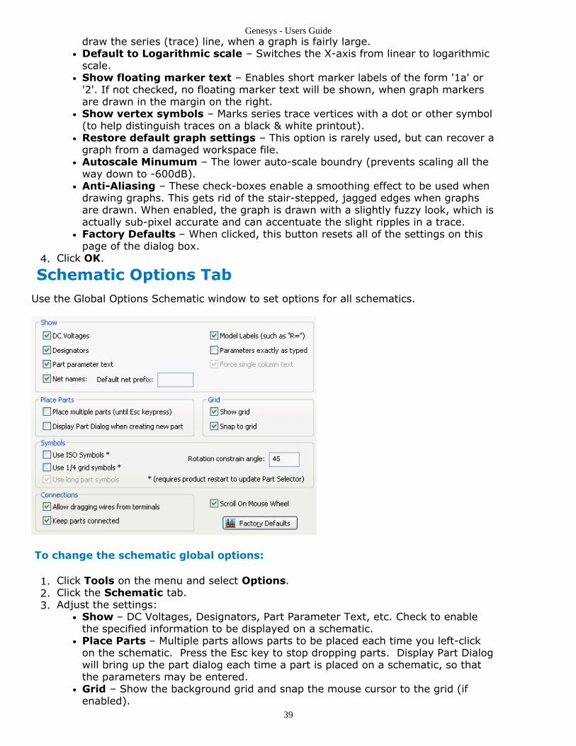
Genesys - Users Guide
39
draw the series (trace) line, when a graph is fairly large.Default to Logarithmic scale – Switches the X-axis from linear to logarithmicscale.Show floating marker text – Enables short marker labels of the form '1a' or'2'. If not checked, no floating marker text will be shown, when graph markersare drawn in the margin on the right.Show vertex symbols – Marks series trace vertices with a dot or other symbol(to help distinguish traces on a black & white printout).Restore default graph settings – This option is rarely used, but can recover agraph from a damaged workspace file.Autoscale Minumum – The lower auto-scale boundry (prevents scaling all theway down to -600dB).Anti-Aliasing – These check-boxes enable a smoothing effect to be used whendrawing graphs. This gets rid of the stair-stepped, jagged edges when graphsare drawn. When enabled, the graph is drawn with a slightly fuzzy look, which isactually sub-pixel accurate and can accentuate the slight ripples in a trace.Factory Defaults – When clicked, this button resets all of the settings on thispage of the dialog box.
Click OK.4.
Schematic Options TabUse the Global Options Schematic window to set options for all schematics.
To change the schematic global options:
Click Tools on the menu and select Options.1.Click the Schematic tab.2.Adjust the settings:3.
Show – DC Voltages, Designators, Part Parameter Text, etc. Check to enablethe specified information to be displayed on a schematic.Place Parts – Multiple parts allows parts to be placed each time you left-clickon the schematic. Press the Esc key to stop dropping parts. Display Part Dialogwill bring up the part dialog each time a part is placed on a schematic, so thatthe parameters may be entered.Grid – Show the background grid and snap the mouse cursor to the grid (ifenabled).

Genesys - Users Guide
40
Symbols – Use ISO symbols: When checked, ISO standard symbols will beplaced. (The ISO standard resistor is a box, instead of a zigzag.) Use ¼ gridsymbols: When checked, it will place ADS-compatible parts that have terminalsspaced on ¼ of the standard part length (which i the length of a resistor). standard parts are on a 1/6th grid spacing. These settings will not take fulleffect until you have exited and restarted. Rotation constrain angle: Sets theF3-key rotation increment (usually 45 or 90 degrees).Connections – Allow dragging wires enables schematic parts to be easilyconnected; just place the mouse cursor over a part terminal, press the left-button, and drag the newly-created connector to another node. Keep partsconnected ensures that schematic parts retain their electrical connections, byinserting new wires (as necessary) when dragging parts. The Alt-key acts as atoggle for the keep connect setting.Scroll On Mouse Wheel – When checked, the mouse center wheel scrolls theschematic window; when unchecked, the wheel zooms the window instead.Factory Defaults – When clicked, this button resets all of the settings on thispage of the dialog box.
Click OK.4.
Layout Options TabUse the Global Layout Options window to specify options for every layout you create.
To change the layout global options:
Click Tools on the menu and select Options.1.Click the Layout tab.2.Adjust the settings:3.
Rotation / Part Constrain Angle – Specifies the allowable incrementatalrotations (usually 45 or 90) for parts on a layout.Layout Mesh Resolution – The default mesh resolution, which is used byMomentumGX.Show Grid – When checked, a grid will be displayed in all layout windows.Scroll On Mouse Wheel – When checked, the mouse center wheel scrolls thelayout window; when unchecked, the wheel zooms the window instead.
Click OK.4.

Genesys - Users Guide
41
Directories Options TabUse the global options directories window to set the default directory paths.
To set the global directory paths:
Click Tools on the menu and Select Options.1.Click the Directories tab.2.Click on Directory Path or label to see a description of what it's used for.3.
To change a path:
Click a Directory Path1.Click Browse2.Select the correct path3.Click OK4.
NoteYou can edit the path directly.
Language Options TabUse the Global Options Language window to select a different language in which to run.The default language is pre-selected for your computer and is listed as Automatic in thiswindow. Other choices include Chinese, Korean, and Japanese. You must restart yourcomputer before any language changes can take effect.

Genesys - Users Guide
42
To change the language global options:
Click Tools on the menu and select Options.1.Click the Language tab.2.Select a language from the Language list.3.Click OK.4.
Default Units Options TabUse the Global Options Units window to make global changes to the default units in aschematic. Changing the default units has no bearing on any of the parts that are in theschematic. Only the initial units of parts placed after the default unit changes are affected.
NotePhysical length is unique. For layout dimensions, the units are specified in the General tab of the LayoutProperties window for each layout.
The global default units used are listed in the table below.
Quantity Units
Angle Degrees
Capacitance pF (picofarads)
Conductance mhos (1/ohms or Siemens)
Current Amps
Frequency MHz (Megahertz)
Inductance nH (nanohenries)
Physical Length, Width, Height mm (millimeters), or based on substrate for netlist
Power dBm (referenced to a milliwatt)
Resistance ohms
Temperature C (Celsius)
Time ns (nanoseconds)
Voltage V (volts)

Genesys - Users Guide
43
NoteAdditional default units are available for non-linear models. They all begin with NL_. The default units forthese parameters are the industry standard units, and you should not need to change them.
To change the global default units:
Click Tools on the menu and select Options.1.Click the Units tab.2.Change the units you want by clicking the Units grid cell next the parameter type3.and selecting the desired unit from the pop-up combo box.Click OK.4.
Appearance Options TabUse the appearance options window to see the default directory paths.
To change the appearance global options:

Genesys - Users Guide
44
Click Tools on the menu and select Options.1.Click the Appearance tab.2.Adjust the settings:3.
Tabbed with splitters – Specifies the use of tabbed view windows, withsplitter bars.Overlapped – Specifies the use of multiple document interface (MDI)overlapping windows.Place close button on tabs – When checked, the tab close button will beplaced on the tab button itself (instead of being placed on the right).Factory Defaults – Restores the original factory values to these settings.
Click OK.4.

Genesys - Users Guide
45
Using Genesys Contents
Analysis (users)Annotations (users)Designs (users)Equations (users)Examining Datasets (users)Graphs (users)Importing/Exporting (users)Layouts (users)LiveReports (users)Managing Libraries (users)Optimization (users)Parts, Models, and Symbols (users)Ports, Connection Lines, and Nets (users)Running Scripts (users)Schematics (users)S-Parameters (users)X-Parameters (users)Sub-Network Models (users)Sweeps (users)Tables (users)Templates (users)Testlink (users)Text Netlists (users)Tuning Variables (users)Yield/Monte Carlo (users)

Genesys - Users Guide
46
AnalysisCircuits and systems can be analyzed in many different ways. When you simulate a circuit,the settings for the analysis determine how the simulation runs. The analysis creates adataset with the simulation results. If an analysis is set to automatically recalculate, it willre-simulate each time you make a change to the schematic design and then click a graphor table dependent on the analysis.
Genesys provides the following analysis engines:
DC Analysis (sim) - Determines the circuit DC operating point.Harbec Harmonic Balance Analysis (sim) - Checks the steady-state performance ofnonlinear circuits and oscillators with excellent frequency resolution.Linear Analysis (sim) - Calculates S-parameters and noise parameters of a circuit,substituting resistive ports for sources.Empower Planar 3D EM Analysis (sim) - Performs a linear analysis based on a layoutusing an electromagnetic simulation.RF Design Kit Spectrasys (sim) - Performs a system-block-level non-linear analysison the entire system to determine if all system-level requirements are met.Testlink (users) - Imports data from instruments to allow measurement comparisonwith models used to develop the network being tested.Cayenne Transient Analysis (sim) - Calculates a circuit response using the SPICE timedomain method.
For more info on theses analyses see the Getting Started with Genesys Simulation (sim)
To add an analysis
Click the New Item button ( ) on the Workspace Tree toolbar and select an1.analysis from the Analyses menu. A new analysis of the selected type will becreated.
Fill in the desired analysis parameters.2.When you click OK or Calculate, the analysis will run and create a data set.3.

Genesys - Users Guide
47
AnnotationsAnnotations include text boxes, arrows, shapes, and controls (widgets) that can be placedon a schematic, graph, or LiveReport to help document a workspace, highlight items ofinterest, etc.
Tools Purpose
Rectangle Draw a square or rectangle.
Ellipse Draw a circle or ellipse
Polygon Draws a filled polygon or unfilled polyline.
Arrow/Line Draw a line or arrow. Change the arrow style by selecting a line and picking an arrow type fromArrows button menu.
Arc Draw a circular arc.
Picture Insert a picture. Use this annotation to add a company logo to a graph, for example. Double-click the new object and select a JPG, GIF, or BMP image file to be displayed. (To allow all usersto see the image, the bitmap file should reside on a network server.)
Text Place text. Text has a number of settings. Double-click a text annotation to set the horizontaland vertical justification (text alignment). The name of the text item can be changed and shownon-screen, which simplifies building a schematic title block.
TextBalloon
Draw a text balloon. This annotation has a "tail" which can be anchored to a data point on agraph, to the page, or not anchored (using the right-button menu).
Button Draw a user button. This annotation can be "clicked" to run a custom script, which is specifiedby double-clicking the outer EDGE of the button control. (The middle of the button runs thescript.)
Slider Draw a slider control. This annotation is linked to a tunable parameter and functions much likethe Tuning Window (users).
Settings Purpose
Fill Color Sets the annotation fill color. Use the 3 color buttons to change the colors of the selectedannotation(s). New annotations will be created using the current colors. The bottom-right colorswatch (with a diagonal slash) is transparent, which specifies an unfilled object.
Line Color Sets the annotation line / border color. The bottom-right color swatch (with a diagonal slash) istransparent, which specifies a object with no outline.
Text Color Sets the annotation text color.
LineThickness
Set the width of borders and lines.
Line Style Set the drawing style of borders and lines (dash pattern, etc.).
Arrows Set the arrow style of lines.
Properties Display the properties window for the selected annotation.
ContentsCreating Annotations (users)Line Annotations (users)Text Annotations (users)Button Annotations (users)Slider Annotations (users)Variable Selector (users)
Creating Annotations
The Annotation button on the Schematic, LiveReport, and Graph toolbars toggles thedisplay of the Annotation toolbar.

Genesys - Users Guide
48
The toolbar provides tools like lines, circles, and text that you can use to point out detailsof interest on a schematic, draw a box around a group of components, etc.
To place an annotation:
Click the various settings buttons (colors, line style, etc.) to adjust the settings for1.newly created annotationsClick an annotation tool button (box, arc, text, etc.) on the Annotation Toolbar.2.Click in a schematic, LiveReport, or graph window to place the new annotation.3.Use the annotation setting buttons to change existing, selected annotations. (More4.than 1 annotation can be adjusted at a time).To set the Font for annotations with text, right-click the object and pick Font... from5.the pop-up menu.
Line AnnotationsLines have many drawing options: Line Thickness, style, color, arrowheads, etc., whichare controlled via the Annotation toolbar and by the object's right button menu. Lines canhave arrowheads and ends. Simply select a line and pick an arrow type:
Arrow Heads Arrow Ends
Text AnnotationsA text annotation is a filled rectangular box with text inside.
To change the properties of a text annotation:
Double-click any text object.1.Make the changes you want.2.Click OK.3.

Genesys - Users Guide
49
Property Purpose
Name The name of the Text object.
Show Name Displays the name of the text item, which simplifies building a adding a titleblock or other "labeled text".
Enter Lines of Text Specifies the test to be displayed.
Font Click the button to set the font.
Justification Sets the horizontal justification (alignment) of the text: Left, Right, or Center.
Vertical Justification Sets the vertical alignment of the text: Top, Bottom, or Vertically Centered.
Horizontal and VerticalMargins
Sets the margins (border gap) of the text. Specified in page coordinates(1/1000ths of an inch).
Tips for advanced users
Text annotations can use equations. For example, if your workspace contains an equationblock with a text variable named CompanyName, you can place =CompanyName in theText field. (The leading = sign indicates that the text string is actually an expression.)When the annotation is drawn, the equation will be evaluated and the result displayed.
Text annotations can display model and parameter info when used within a customsymbol . This is implemented via macro-text-substitution. When symbol text is drawn ona schematic, the displayed text is modified prior to output. For example, Name=%Model%would be displayed as "Name=Resistor" on a symbol using a resistor model. Therecognized macro strings are:
%Des% - Displays the part's designator.1.%Model% - Displays the name of the model attached to the part.2.%MODEL% - Displays the model name in UPPERCASE.3.%ParameterName% - Displays the value of the specified model parameter4.attached to the part. E.g. R, C, L, QL, MODE, etc.
Button Annotations (Widgets)A button annotation is a control which runs a script when clicked. Buttons and other

Genesys - Users Guide
50
widgets are initially created using "stock Windows colors"; the controls' colors can easilybe changed using the Annotation toolbar, as can line thickness, etc.
To change the properties of a button:
Double-click the EDGE of any button object.1.Make the changes you want.2.Click OK.3.
Property Purpose
Caption The title text displayed on the button.
Script Commands Specifies the script to be run, when the button is clicked.
Font To set the font.
Shape Buttons can be a rectangle, a rounded rectangle, or an ellipse.
Disabled Grays and inactivates the button.
Slider Annotations (Widgets)A slider annotation is a control which adjusts a tunable equation variable, part parameter,etc. Sliders and other widgets are initially created using "stock Windows colors"; thecontrols' colors can easily be changed using the Annotation toolbar, as can line thickness,etc.
To change the properties of a slider:
Double-click the EDGE of any slider object.1.Make the changes you want.2.Click OK.3.

Genesys - Users Guide
51
Property Purpose
Variable The variable to be tuned.
'...' Button Brings up a selector to pick the variable.
Min and Max Specifies the limits of the tuning range. These can be set to the names of equationvariables, for adjustable limits.
Units Displays the units of the tune variable.
Number of Tics The number of slider division marks.
Orientation Sliders can be horizontal or vertical.
Slider Labels Specifies what text (if any) to display on a slider.
Show / Hide All Check or uncheck all the Show checkboxes.
Run simulations Runs enabled simulations on left-button up.
Display long variablename
Displays the tune variable's long name (Eg: Project\Sch1\L1.L).
Hide name prefix Omits the part or equtaion name (Eg: L instead of L1.L).
Disabled Grays and inactivates the slider.
Snap to integervalues
Limits the tuning to integer values.
Variable SelectorThis is displayed via the '...' button.

Genesys - Users Guide
52
Property Purpose
Filter by Limits the variables displayed to only those that include the specifiedtext.
Variable Displays the variable's name.
Path Displays the full pathname of the variable.
Value Displays the current value of the variable.
Tuned Displays an X, if the variable is tunable.
Part parameters only Limits the variables displayed to only part parameters.
Show tuned variables only Limits the variables displayed to only tunable variables.
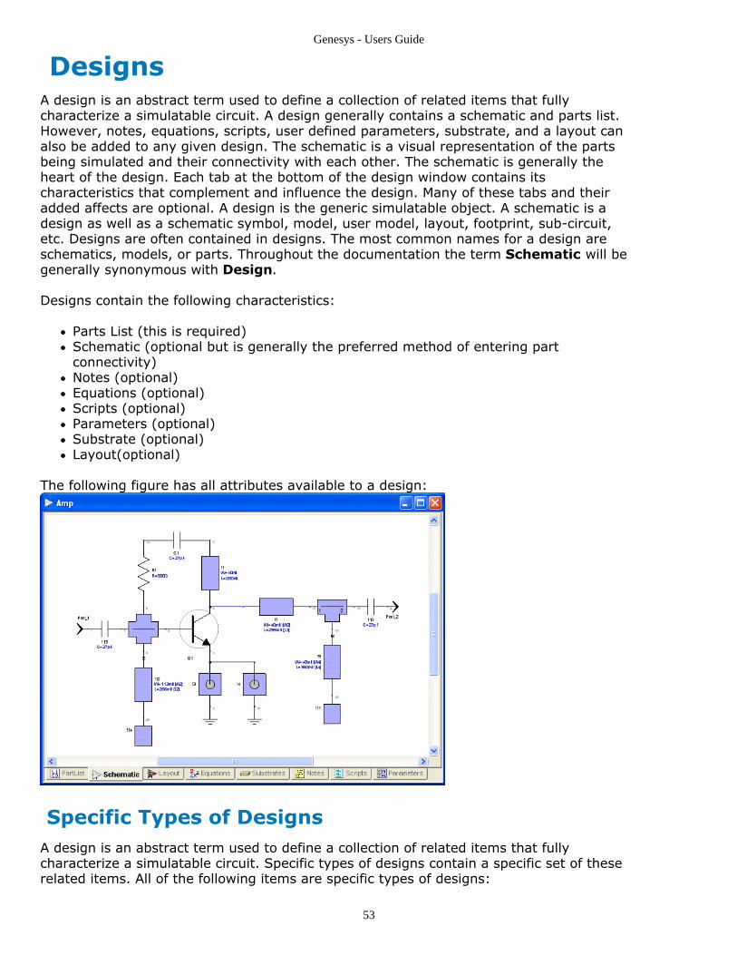
Genesys - Users Guide
53
DesignsA design is an abstract term used to define a collection of related items that fullycharacterize a simulatable circuit. A design generally contains a schematic and parts list.However, notes, equations, scripts, user defined parameters, substrate, and a layout canalso be added to any given design. The schematic is a visual representation of the partsbeing simulated and their connectivity with each other. The schematic is generally theheart of the design. Each tab at the bottom of the design window contains itscharacteristics that complement and influence the design. Many of these tabs and theiradded affects are optional. A design is the generic simulatable object. A schematic is adesign as well as a schematic symbol, model, user model, layout, footprint, sub-circuit,etc. Designs are often contained in designs. The most common names for a design areschematics, models, or parts. Throughout the documentation the term Schematic will begenerally synonymous with Design.
Designs contain the following characteristics:
Parts List (this is required)Schematic (optional but is generally the preferred method of entering partconnectivity)Notes (optional)Equations (optional)Scripts (optional)Parameters (optional)Substrate (optional)Layout(optional)
The following figure has all attributes available to a design:
Specific Types of DesignsA design is an abstract term used to define a collection of related items that fullycharacterize a simulatable circuit. Specific types of designs contain a specific set of theserelated items. All of the following items are specific types of designs:

Genesys - Users Guide
54
SchematicSchematic SymbolUser ModelFootprintLayout
ContentsCreating a Design (users)Modifying a Design (users)Design Properties (users)Using Design Wizard (users)
Design Properties
General Tab
Use the General Properties tab page to change the general properties of a Design.
Name - The name of the Design.Description - The Design description (optional).Intended Use - What kind of Design is it? This setting controls the Design's icon onthe workspace tree and Genesys' interpretation of how the design is intended to beused. (If it's a symbol, you can select it for a schematic part's symbol, if it's a model,you will be able to select it as a model, etc.)
Modifying a DesignThe following attributes can be added to a design:
NotesEquationsScriptsParameters

Genesys - Users Guide
55
SubstrateLayoutHere is a brief overview of these attributes.
Notes
A note can be added to help document different aspects of the design.
Equations
An equation block can be added to a design so that variables can be based on equations.These variables can be used for various design parameters. An equation block is generallythe link between the parameters a user would see and the parameters used in models.
NoteThese equations are local to the design. Other parts of your workspace cannot access the variables in thisequation set.
For more information see Equations (users).
Scripts
Scripts control Genesys operations. Add a script to your design to load files, save files,save data sets, and change object parameters.
NoteTo run this script, copy the text and paste it into the Script Processor, then selectRun.
For more information see Running Scripts (users).
Parameters
Parameters are added to a design when the implementation details are generally hiddenfrom the user as is the case of a user model. When a design contains parameters thisdesign can be used as a user model and these parameters will be exposed as modelparameters in the part that uses this design as its model.
For more information see User Defined Parameters (users).
Substrate
Designs can contain any number of local substrates. This is used mainly when creatingmodels so that a model can have an underlying substrate. When your model looks for asubstrate it will look first in the Substrates container in the design and then in theworkspace. Other designs can not access substrates in this design's local container.
Adding a Design Attribute
To add one of these attributes to a design right click on one of the tabs at the bottom ofthe design and select the desired attribute.

Genesys - Users Guide
56
Deleting a Design Attribute
A tab can also be deleted from a design my right clicking on it and selecting the 'Delete'menu entry.
Creating a DesignThere are two different ways to to create a design in Genesys. One is the by clicking on
the New Item button ( ) on the Workspace Tree toolbar or by right clicking on afolder in the workspace tree.
Method 1 - Clicking on the New Item Button
Click the New Item button ( ) on the1.
Workspace Tree toolbarSelect the 'Designs >' submenu2.Now select the design of interest3.The design will added under the folder that4.last selected in the workspace tree
Method 2 - RightClicking on a WorkspaceFolder
Right click on a1.folder in theworkspace tree tobring up the rightclick menu.Select the 'Add >'2.submenu.Select the 'Designs3.>' submenuNow select the4.design of interestThe design will5.added under thefolder that wasinitially right clicked
NoteIf you create the new design in the wrong folder, simply drag it to the folder of interest.
Using the Design WizardThe Design Wizard makes designing easier if you are new to Genesys or if you want toautomate the design process.

Genesys - Users Guide
57
To create a design using the Design Wizard:
Click the New Item button on the Workspace Tree toolbar and select Design1.Wizard from the Designs menu.
Type a name for the design in the Enter the New Design's Name box.1.Click a button to specify whether you want to base your design on an existing2.design, a blank schematic, a blank layout, or another kind of design.Do one of the following:3.
Click Finish if you selected to base your design on a blank schematic or ablank layout.Click Next if you selected to base your design on an existing design oranother type design.
If you selected Based on a Design in an Existing Library, do the following:4.Select the name of the library from the Select the Library Which Containsthe Prototype list.Select a prototype from the Select a Prototype list.
If you selected Another Kind of Design, do the following:5.Click one of the buttons to indicate your intended use for the design.Click Next.Click any of the boxes to select initial components to add to your design.Click Finish.

Genesys - Users Guide
58
EquationsEquations are a powerful tool that enable post processing of data, control over inputs tosimulations, and definition of user-defined custom models. Two languages are availablefor defining equations: Engineering Language (EngLang) and Mathematics Language(Math Language).
ContentsEquations User Interface (users)Languages (users)Hierarchy in Equations (users)Automatic Calculation (users)Debugging Equations (users)Tips for Effective Equation Writing (users)
Using Engineering LanguageEngineering Language is a simple programming language with structured controlstatements. Variable types are defined in context and matrices and arrays can be easilymanipulated with equations.
For a full description see Using Engineering Language (users).For a complete function reference see Engineering Language Function Reference(users)
Using Math LanguageMath Language, along with most of its built-in functions, was designed to be compatiblewith m-file script syntax.
For a full description see Using Math Language (users).For a complete function reference see Math Language Function Reference (users)
Comparing Engineering Language and Mathematics Languages
There are two languages available to use in Equations. Which one should you choose?
Engineering Language is well suited for interacting with the workspace and for ease ofuse, while Mathematics Language gives you full control over array processing.Mathematics language is the more powerful and flexible language, and those familiar withMATLAB m-file syntax will prefer to use Mathematics Language. In Engineering Language,it is simpler to access dataset variables ( Dataset.Var is how you would access a variableVar in a dataset called Dataset), and it understands Swept variables and provides someflexibility in dealing with them.
Mathematics language is syntactically compatible with M-files. It has a lot of power fornumeric processing. In some common cases, Mathematics Language code can be moreverbose than Engineering Language. For example, if a Linear Analysis produces a swept2x2 S-matrix of 100 frequencies, EngLang would understand that S[2,1] means S21 for allfrequencies. In Math Language, you must explicitly specify that you want all frequenciesby using the syntax S(:,2,1). However, there are some places where Mathematics

Genesys - Users Guide
59
Language is more compact, allowing things like 1+3j for a complex number, or 1/Var toinvert a matrix. Also, Mathematics Language includes support for file I/O and tcp/ipcommunication functions, both of which are not supported in Engineering Language.
The two equation languages can talk to each other's variables (and the Math Languagemay retain units and dependencies when you use an EngLang variable). They do not sharefunctions because they are syntactically different (Math Language can return multipleresults, for example).
Select which language is being used by an equation set by picking from the Math or Engbutton pulldown in the Equation window.
Here is a simple comparison of Engineering Language vs. Mathematics Language:
Feature EngLang MathLang
Shortcuts for common vars (eg. S21) X
Read/write to/from Datasets X X
Run Analysis from a script X X
Array-assignments X
File I/O functions X
TCP/IP Comm (Instrument connectivity) X
Signal Processing functions X
Multiple return values for functions X
Engineering Language Function ReferenceTo go directly to entries that start with a specific letter, select one of the following: A, B, C, D, E, F, G, H, I, K, L, M, N, O, P, Q, R, S, T, U, V, Z.
Function Name Description
abs (users) Magnitude of a number x.
abssum (users) Sums the magnitude of each part in x.
ang (users) Phase of a complex number x in radians.
ang360 (users) Phase of a complex number x in radians.
acos (users) Inverse cosine of x.
acosh (users) Inverse hyperbolic cosine of x.
array (users) builds an array with dimensions x by y by ... (can take in any number of arguments,but at least 1).
asin (users) Inverse sine of x.
asinh (users) Inverse hyperbolic sine of x.
atan (users) Inverse tangent of x.
atanh (users) Inverse hyperbolic tangent of x.
beta (users) Evaluates the Beta function for corresponding parts of z and w, which must be non-negative real values.
betacdf (users) Returns the cumulative distribution function of the Beta distribution with parameters a

Genesys - Users Guide
60
and b evaluated at theparts of x.
betainc (users) Evaluates the incomplete Beta function for corresponding parts of x, z, and w. x mustbe between 0 and 1. z andw must be non-negative real values.
betainv (users) Returns the inverse of the Beta cumulative distribution function with parameters a andb evaluated at the parts of p.
betaln (users) Evaluates the natural logarithm of the Beta function for corresponding parts of z andw, which must be non-negativereal values.
betapdf (users) Returns the probability distribution function of the Beta distribution with parameters aand b evaluated at the parts of x.
ceil (users) Returns the smallest integer greater than or equal to x. If x is complex, only the realpart is used.
column (users) Force a row or column vector x to be a column vector.
complex (users) Returns the complex number x + jy.
concatcolumns (users) Concatenates matrices or vectors x and y. The number of rows of x and y must beequal.
conj (users) Complex conjugate of x.
cos (users) Cosine of x, where x is in radians.
cosh (users) Hyperbolic cosine of x.
cp (users) Process capability index.
cpk (users) Process capability index accounting for the mean.
cplower (users) Lower process capability index.
cpupper (users) Upper process capability index.
db (users) x expressed in decibels as 20*log(x).
db10 (users) x expressed in decibels as 10*log(x).
dbm (users) Returns the dBm equivalent of x Watts.
dbmtow (users) Returns the Watts equivalent of x dBm.
dbpolar (users) Returns the complex value of a voltage in dB and the angle in degrees.
derivative (users) returns a vector that is the derivative at each point of the dependent with respect toindependent vector.
dev_lin_phase (users) returns a vector in radians of deviation from linear phase; this function is a clone ofthe ADS function by the same name.
diag (users) If the argument is a matrix, this returns a vector with the diagonal parts. Otherwise,the argument must be a vector,and diag creates a matrix with the vector on the diagonal and all other parts zero.
erf (users) Computes the error function of each part x.
erfc (users) Computes the complementary error function of each part of x.
exp (users) e to the power of x, where e = 2.7182817...
eye (users) Function to build an eye diagram from transient data. symbolRate is in Hz, numCyclesis the number of cycles to plot beforewrapping (optional), and delay is the number of samples of delay (optional).
fft (users) Discrete Fourier Transform (DFT) of data, computed with FFT algorithm when possible. The len argument (the FFT Length) isoptional.
floor (users) Returns the largest integer less than or equal to x. If x is complex, only the real partis used.
gamma (users) Evaluates the Gamma function for each part of x, which must be real.
gammainc (users) Evaluates the incomplete Gamma function for each part of x, which must be real.
gammaln (users) Evaluates the natural logarithm of the Gamma function for each part of x withoutcomputing the Gamma function itself.
gammatoz (users) Returns the complex impedance given the normalizing impedance and the voltagereflection coefficient (gamma).

Genesys - Users Guide
61
getdbunit (users) Returns the appropriate dB unit: RelDB10 if the input units are power or RelDB20 ifthe input units are voltage/current.
getindep (users) Returns the string property containing the path to the independent value of a variablex. (ie. the reference to the independentvariable)
getindepvalue (users) Returns the value of the independent variable of a variable x. x must have only oneindependent value.
getunits (users) Returns an integer corresponding to the units of a variable x. This integer may beused by setunits.
hb_gain (users) Calculates the complex gain for selected spectral component.
hb_getspcomp (users) Returns the complex amplitude of the spectral component in Watts.
hb_getspcompdbm(users)
Returns the amplitude of the spectral component in dBm.
hb_iipn (users) Returns the input intercept point of two components IndexS1 and IndexS2 of thepower spectrum SpectrPout.
hb_ipn (users) Calculates the common part of the input and output intercept point functions (hb_iipnand hb_oipn).
hb_larges (users) Calculates the Large Signal S-parameter for a 1-tone HB analysis.
hb_largesmix (users) Calculates the LargeSignal S-parameter for multi-tone HB analyses.
hb_oipn (users) Calculates the output intercept of the two components IndexS1 and IndexS2 of thepower Spectrum SpectrPout.
hb_spurious (users) Calculates the max amplitude of spurious spectral components in the spectrumSpectrVout.
hb_totalsp (users) Calculates total amplitude for spectral components having the same frequency andsets all of them to the same total amplitude.
hb_transgain (users) Calculates the transducer gain.
hb_transgaindb(users)
Calculates the transducer gain in dB.
histogram (users) creates bins for the data in x and returns the number of parts in each container.
hermitian (users) conjugate transpose of a matrix or swept matrix x
identity (users) Returns an nxn identity matrix. (Datatype is Complex)
iff (users) Returns value1 if boolean expression is true, otherwise value2.
ifft (users) Inverse Discrete Fourier Transform (IDFT) of data, computed with IFFT algorithmwhen possible. The len argument (IFFT length)is optional.
iftrue (users) If x is true, return y. x and y may be vectors.
imag (users) Imaginary part of a (complex) number x.
im (users) Same as imag(x).
integrate (users) Numerically integrate the dependent with respect to independent, from index = startto index = stop.
interpolate (users) Produces an array where the independent value of var is changed to new_indep,interpolating as necessary.
intersect (users) Produces a vector representing a set which is the intersection of two sets (vectors) xand y.
inverse (users) Returns the inverse of a non-singular matrix x.
kurtosis (users) Returns the sample Kurtosis of x.
largeS (users) returns the largeSij for this HB dataset
lininterp (users) Returns the linear interpolation of the output values given the data values of indepand dep.
ln (users) Natural logarithm of x.
log (users) Logarithm (base 10) of x.
mag (users) Same as abs(x).
matrix (users) Builds an x by y matrix of complex numbers. parts are initialized to zero.

Genesys - Users Guide
62
max (users) Returns the maximum (magnitude) part of any array x on the dimension iDim.
mean (users) Returns average of all parts in a vector or an array on the dimension iDim.
median (users) Returns the median of all parts in a vector or an array on the dimension iDim.
min (users) Returns the minimum (magnitude) part of any array x on the dimension iDim.
mode (users) Returns the mode of all parts in a vector or an array on the dimension iDim.
moment (users) Returns the central moment of order order of a vector x.
ndim (users) Number of dimensions of an array x.
nftovni (users) Converts noise factor into an equivalent input noise resistance.
norm (users) Magnitude-squared of a complex number x.
normcdf (users) Returns the cumulative distribution function of the normal distribution with mean muand standard deviation sigma evaluated atthe values of x.
norminv (users) Returns the inverse cumulative distribution function of the normal distribution withmean mu and standard deviation sigma evaluatedat the values of x.
normpdf (users) Returns the probability distribution function of the normal distribution with mean muand standard deviation sigma evaluated at thevalues of x.
numcols (users) Returns the number of columns in a matrix x.
numrows (users) Returns the number of rows in a matrix x.
ones (users) if n argument is omitted: generate a vector of m 1's, otherwise generate an mxnmatrix of 1's.
posterror (users) Converts the argument to a string (if necessary) and posts the string to the error log.The error stays on the log until the equationsare recalculated. This causes the equations to error out and not calculate, as well asposting the error.
postwarning (users) Converts the argument to a string (if necessary) and posts the string to the error logas a warning. The warning stays on the log untilthe equations are recalculated. This does not cause the equations to error out. Theequations will calculate.
pow (users) Returns x to the power of y.
prctile (users) Returns the p'th percentiles of a vector x (p can be a scalar or a vector of percentvalues).
prod (users) Calculates the product of all the parts in x.
quantile (users) Returns the q'th quantiles of a vector x (q can be a scalar or a vector of quantilevalues).
rand (users) Generate uniformly distributed random numbers on the interval [0, 1). Botharguments are optional. If both arguments are omitted,the function returns a random scalar. If the second argument is omitted, generate avector of m random numbers. Otherwise, generatean mxn matrix of random numbers.
randn (users) Generate Gaussian distributed random numbers with mean 0 and variance 1. Botharguments are optional. If both arguments areomitted, the function returns a random scalar. If the second argument is omitted,generate a vector of m random numbers. Otherwise,generate an mxn matrix of random numbers.
real (users) Real part of a (complex) number x
re (users) Same as real(x)
reshape (users) sets the dimensions of the variable x to be that described by newshape. Swept-dimensions are NOT counted. (eg. if S is the variableproduced by a 100 point linear analysis of a 2-port circuit, reshape(S, [4;1]) wouldreturn a variable containing S, but havingdimensions 100x4x1)
resize (users) sets the dimensions of the variable x to be that described by newshape. Swept-dimensions are counted. (eg. if S is the variableproduced by a 100 point linear analysis of a 2-port circuit, resize(S, [100;4;1]) would

Genesys - Users Guide
63
return a variable containing S, but havingdimensions 100x4x1)
reverse (users) returns the reverse of a vector, so [1,2,3,4] becomes [4,3,2,1]; for matrices this willreverse the columns
rltogamma (users) Returns the voltage reflection coefficient (gamma) based on the return loss in dB andthe angle in radians
rltoz (users) Returns the complex impedance based on the normalizing impedance, return loss indB and the angle in radians
rotate (users) rotates a vector by the integer rotate; if vector = [1,2,3,4], rotate(vector,2) returns[3,4,1,2]; for matrices this will rotatethe rows.
RsCondToThick(users)
Returns metal thickness in defined by string parameter Tunits units;RsCondToThick(Rs,Cond,Tunits);Rs - sheet resistance Ohm/Sq, Cond - conductivity Ohm*MExamples: T_mil=RsCondToThick(50,5.8e7,"mil");T_mm=RsCondToThick(50,5.8e7,"mm")
RsResToThick (users) Returns metal thickness in defined by string parameter Tunits units;RsResToThick(Rs,Res,Tunits);Rs - sheet resistance Ohm/Sq, Res - resistivity Ohm*MExamples: T_mil=RsResToThick(50,1.724e-8,"mil"); T_mm=RsResToThick(50,1.724e-8,"mm")
RsRhoToThick (users) Returns metal thickness in defined by string parameter Tunits units;RsRhoToThick(Rs,Rho,Tunits);Rs - sheet resistance Ohm/Square, Rho=Res/ResCop - relative to copper resistivityRes, where copper resistivity ResCop=1.724e-8 Ohm*MExamples: T_mil=RsRhoToThick(50,1000,"mil");T_mm=RsRhoToThick(50,1000,"mm")
runanalysis (users) Run an analysis in the workspace tree
setindep (users) set the independent reference for a swept dependent variable to indepvar(s). Aminimum of two arguments is required.This function can be used to remove all independent values of a variable by passing ina blank string for the second argument.
setplottype (users) sets the plot-type property of a variable. Valid plot types include "" (Empty string),"Discrete", "Spectrum", "Level", "Spur","SpurFree", "OutOfRange", "ValidIF", "Contour", "PointPlot", and "Histogram".
setunits (users) sets a variable named varname to have units specified by unit. unit may be aninteger or a string. Example setunits( "totaltime","msec")or setunits( "frqsweep", "MHz"). The units are used to by graphs to determine the axislabels and values. They can also by used by theTune window. Use UseMKS if you are settings units of variables manually to avoidconfusion.
shape (users) Returns a vector containing the number of parts in each dimension of x. Swept-dimensions are NOT counted. (eg. if S is thevariable produced by a 100 point linear analysis of a 2-port circuit, shape(S) returnsthe vector [2;2] ).
sin (users) Sine of x, where x is in radians.
sinc (users) Sin(x)/ x, or 1 if x = 0.
sinh (users) Hyperbolic sine of x.
size (users) Returns a vector containing the number of parts in each dimension of x. Swept-dimensions are counted. (eg. if S is thevariable produced by a 100 point linear analysis of a 2-port circuit, size(S) returns thevector [100;2;2] ).
skewness (users) Returns the sample skewness of a vector x.
sort (users) Sorts a vector x in ascending order.
std (users) Calculates the standard deviation of x.
sqr (users) Square-root of x.
sqrt (users) Same as sqr(x).

Genesys - Users Guide
64
stoy (users) convert S-parameters to Y-parameters
stoz (users) convert S-parameters to Z-parameters
stos (users) renormalize S-parameters to a different impedance
substrateer (users) return the dielectric constant (Er) of the substrated named SubstName.
substratetand (users) return the loss tangent of substrate named SubstName.
substraterho (users) return the relative resistivity of substrate named SubstName.
substratetmet (users) return the metal thickness of substrate named SubstName.
substraterough(users)
return the surface roughness of substrate named SubstName.
substrateh (users) return the height of substrate named SubstName.
sum (users) Calculates the sum of all the parts of x on the dimension iDim.
tan (users) Tangent of x, where x is in radians.
tanh (users) Hyperbolic tangent of x.
tcdf (users) Returns the cumulative distribution function of the Student's T distribution withdegrees of freedom parameter v evaluated at theparts of x.
tinv (users) Returns the inverse of the cumulative distribution function of the Student's Tdistribution with degrees of freedom parameter vevaluated at the parts of p.
time (users) constructs a time-domain waveform from complex spectra at arbitrary frequencies. (Eg: time( V1, Freq, Time) where V1, Freq, and Time are variables in a HarBECDataset)
times (users) Returns the part-by-part product of the two arguments. If one entry is a scalar andone is an array, the return value isthe scalar multiplied by every part in the array. This is in contrast to the * operatorthat does matrix multiplication.
timevector (users) Creates a vector of times from start to stop with a specified step size.
tpdf (users) Returns the probability distribution function of the Student's T distribution withdegrees of freedom parameter v evaluated atthe parts of x.
transpose (users) Transposes a matrix or swept matrices x
union (users) Produces a vector representing a set which is the union of two sets (vectors) x and y
englang_unwrap(users)
returns a vector of unwrapped phase; both input and output of the function areradians (note that ang() returns radians sothis is already self-consistent; z = unwrap( ang(Linear1.S[2,1]) ) is an example.
using (users) sets the current context in an equation block to the dataset called Dataset.
var (users) Calculates the variance of x.
vector (users) Builds a vector of complex numbers of length x. parts are initialized to zero.
zeros (users) if n argument is omitted: generate a vector of m 0's, otherwise generate an mxnmatrix of 0's
absSyntaxy = abs(x)
Definitionabs takes the absolute value of a real variable or the magnitude of a complex variable.Same as mag function
Examples:

Genesys - Users Guide
65
Formula Result
abs( -1.5) 1.5
abs( complex( 1,1) ) 1.414
abs( [-1;-2;3] ) [1;2;3]
CompatibilityNumeric scalars, Vectors, Arrays
See Alsomag (users)
abssumSyntax
y = abssum(x)
Definition abssum calculates the absolute value of each part in x and returns the sum of thoseparts. If an part in x is a complex number then the magnitude of the part is used in thesummation.
Examples:
Formula Result
x = [ -2.1 , 3.4 , 5.6 ]y = abssum(x)
11.1
x = [ complex(1,-.4), complex(-1,1) ]y = abssum( b )
2.491
CompatibilityNumeric scalars, Vectors, Arrays
See Alsoabs (users)
acosSyntax y = acos(x)
Definition acos returns the inverse cosine of the number, in radians (MKS) between 0 <= r <= PI
Examples:
Formula Result or
acos( 0 ) 1.571 PI/2
acos( 1 ) 0 0
acos( -1 ) 3.141 PI
acos( .707) 0.786 PI/4
acos( -.707) 2.356 3*PI/4
CompatibilityNumeric scalars, Vectors, Arrays
See Also

Genesys - Users Guide
66
asin (users)
acoshSyntax y = acosh(x)
Definition acosh returns the inverse hyperbolic cosine of the number, or log( x + sqrt( x2 - 1)).acosh takes magnitude of a complex argument before evaluating.
Examples:
Formula Result
acosh( 1 ) 0
acosh( 10 ) 2.993
acosh( 0) undefined
CompatibilityNumeric scalars, Vectors, Arrays
See Also
asinh (users)atanh (users)
angSyntax y = ang(x)
Definition ang finds the angle of a complex number. The range of y is -180 to 180 degrees;internally, the number is stored in radians (MKS), but since the unit is ANGLE, the valuecan be displayed in degrees or radians. (This differs from ang360, which returns aunitless value.)
Examples:
Formula Result
ang( 1) 0
ang( complex( sqr( 3 ) / 2 , .5) ) 0.524
ang( complex( 1,1) ) .785
CompatibilityNumeric scalars, Vectors, Arrays
See Alsoang360 (users)
ang360

Genesys - Users Guide
67
Syntax y = ang360(x)
Definition ang360 finds the angle of a complex number in degrees. The range of y is 0 to 360;ang360 specifically returns a unitless value (unlike ang, which returns a value withANGLE units).
Examples:
Formula Result
ang360( 1) 0
ang360( complex( sqr( 3 )/2 , .5) ) 30
ang360( complex( 1,1) ) 45
CompatibilityNumeric scalars, Vectors, Arrays
See Alsoang (users)
arraySyntax y = array( a, b, ...)
Definitionarray creates a multidimensional complex array. The argument list must have at least oneinteger (to produce a vector). All arguments are set to zero.
Examples:
Formula Result
array( 2 ) a 2 part vector
array( 3, 4, 5 ) a 3 dimensional array of size 3x4x5
CompatibilityVariable length integer list
See Also
reshape (users)shape (users)
asinSyntax y = asin(x)
Definition asin returns the inverse sine of the number, in radians (MKS) between -PI / 2 <= r <= PI/ 2
Examples:

Genesys - Users Guide
68
Formula Result or
asin ( 0 ) 0 0
asin ( 1 ) 1.571 PI/2
asin( -1 ) -1.571 -PI/2
asin ( .707) 0.786 PI/4
asin ( -.707) -0.786 -PI/4
CompatibilityNumeric scalars, vectors, arrays
See Alsoacos (users)
asinhSyntax y = asinh(x)
Definition asinh returns the inverse hyperbolic sine of the number, or log( x + sqrt( x2 + 1)). asinhtakes magnitude of a complex argument before evaluating.
Examples:
Formula Result
asinh( 1 ) 0.881
asinh( 10 ) 2.998
asinh( 0) 0
CompatibilityNumeric scalars, vectors, arrays
See Also
acosh (users)atanh (users)
atanSyntax y = atan( x )
Definition atan returns the inverse tangent of the number, in radians (MKS) between -PI/2 < r <PI/2
Examples:
Formula Result or
atan( 0 ) 0
atan( 1 ) 0.785 PI/4
atan( -1 ) -0.785 -PI/4
atan( .5) 0.464
atan( -.5) -0.464
Compatibility

Genesys - Users Guide
69
Numeric scalars, Vectors, Arrays
See Alsotan (users)
atanhSyntax y = atanh( x )
Definition atanh returns the inverse hyperbolic tangent of the number, or 0.5 * log( (1 + x) / (1 -x) ). atanh takes magnitude of a complex argument before evaluating.
Examples:
Formula Result
atanh( 1 ) undefined
atanh( .5 ) 0.549
atanh( -.5 ) -0.549
atanh( 0 ) 0
CompatibilityNumeric scalars, Vectors, Arrays
See Alsotanh (users)
betaSyntax y = beta(z, w)
DefinitionEvaluates the Beta function for corresponding parts of z and w, which must be non-negative real values. Both must be of equal dimensions, or either one can be a scalar.
The Beta function is defined as the integral from 0 to 1 of t^(z-1)*(1-t)^(w-1) dt.
Examples:
Formula Result
beta( 1.5, 2 ) 0.2667
beta( [3, 4, 5], 3 ) [0.0333, 0.0167, 0.0095]
CompatibilityNumeric scalars, Vectors, Arrays
See Also
gamma (users)gammaln (users)gammainc (users)betaln (users)betainc (users)
betacdf

Genesys - Users Guide
70
Syntaxy = betacdf(x, a, b)
DefinitionReturns the cumulative distribution function of the Beta distribution with parameters a andb evaluated at the parts of x. All inputs must match in dimensions or be scalars. Scalarsare treated as constant arrays of size compatible with the other arguments.
Examples:
Formula Result
betacdf( 0.5, 1, 1.5) 0.6464
betacdf( 0.8, [1, 2], 3) [0.992, 0.9728]
CompatibilityNumeric scalars, Vectors, Arrays
See Also
betapdf (users)betainv (users)
betaincSyntax y = betainc(x, z, w)
DefinitionEvaluates the incomplete Beta function for corresponding parts of x (which must bebetween 0 and 1), z, and w, which must be non-negative real values. The argumentsmust be of equal dimensions, or any one can be a scalar.
The incomplete Beta function is defined as (1 / beta(z, w)) times the integral from 0 to xof t^(z-1)*(1-t)^(w-1) dt.
Examples:
Formula Result
betainc( 0.5, 1.5, 2 ) 0.6187
betainc( 0.8, [3, 4, 5], 3 ) [0.9421, 0.9011, 0.852]
CompatibilityNumeric scalars, Vectors, Arrays
See Also
gamma (users)gammaln (users)gammainc (users)beta (users)betaln (users)
betainvSyntaxx = betainv(p, a, b)

Genesys - Users Guide
71
DefinitionReturns the inverse of the Beta cumulative distribution function with parameters a and bevaluated at the parts of p. All inputs must match in dimensions or be scalars. Scalarsare treated as constant arrays of size compatible with the other arguments.
Examples:
Formula Result
betainv( 0.5, 1, 1.5) 0.37
betainv( 0.8, [1, 2], 3) [0.4152, 0.5825]
CompatibilityNumeric scalars, Vectors, Arrays
See Also
betapdf (users)[ betacdf]
betalnSyntax y = betaln(z, w)
DefinitionEvaluates the natural logarithm of the Beta function for corresponding parts of z and w,which must be non-negative real values. Both must be of equal dimensions, or either onecan be a scalar.
Since the Beta function can range over huge values, it is sometimes preferable to use itslogarithm.
Examples:
Formula Result
betaln( 1.5, 2 ) -1.3218
betaln( [3, 4, 5], 3 ) [-3.4012, -4.0943, -4.654]
CompatibilityNumeric scalars, Vectors, Arrays
See Also
gamma (users)gammaln (users)gammainc (users)beta (users)betainc (users)
betapdfSyntaxy = betapdf(x, a, b)
DefinitionReturns the probability distribution function of the Beta distribution with parameters a andb evaluated at the parts of x. All inputs must match in dimensions or be scalars. Scalars

Genesys - Users Guide
72
are treated as constant arrays of size compatible with the other arguments.
Examples:
Formula Result
betapdf( 0.5, 1, 1.5) 1.0607
betapdf( 0.8, [1, 2], 3) [0.12, 0.384]
CompatibilityNumeric scalars, Vectors, Arrays
See Also
betacdf (users)betainv (users)
ceilSyntaxy = ceil( x )
Definitionceil returns the smallest integer greater than or equal to x. If x is complex, only the realpart is used.
Examples:
Formula Result
ceil( 10 ) 10
ceil( complex ( 1.5 , 6 ) ) 2
ceil( [ -0.5, 0.5 ] ) [ 0 , 1 ]
CompatibilityNumeric scalars, vectors, arrays
See Alsofloor (users)
columnSyntaxy = column(x)
DefinitionCreates a column vector y from a row or column vector x. A column vector has onecolumn and one or more rows.
Examples:
Formula Result
x = [1,2,3,4,5]y = column(x) y = [1;2;3;4;5] (vector of 5 rows and 1 column)
CompatibilityVectors
See Alsotranspose (users)

Genesys - Users Guide
73
complexSyntaxz = complex( x, y )
DefinitionReturns a complex number in the form x + jy. The complex number(s) are stored as z = (x2 + y2)(1/2). By default the magnitude of the complex number(s) will be displayed intables and datasets. complex( x, y ) can be used on vectors or matrices of samedimensions.
Examples:
Formula Result
complex( 1 , 1 ) 1 + j = 1.414
complex( 1 , -4 ) 1 - j4 = 4.123
complex( [ 0 , 5 ] , [ 3 , 0 ] ) [ 3 , 5 ]
complex( 5 , 0 ) 5
CompatibilityNumeric Scalars, Vectors, Arrays
See Alsomag (users)
concatcolumnsSyntaxz = concatcolumns( x, y )
DefinitionConcatenates x and y. Variables x and y must have the same number of rows, becompatible data types, and have no more that two dimensions.
Examples:
Formula Result
x = [ 1 , 2 ]y = [ 3 , 4 ]z = concatcolumns( x , y )
z = [ 1 , 2 , 3 , 4 ]
x = [ 1 ; 3 ; 5 ]y = [ 2 ; 4 ; 6 ]z = concatcolumns( x , y )
z = [ 1, 2 ; 3 , 4 ; 5 , 6 ]
Compatibility*. Numeric Scalars*. array (users)*. vector (users)
conjSyntaxy = conj( x )
DefinitionCalculates the complex conjugate of x, where x is a complex number. The conjugate of x+ jy is x - jy.

Genesys - Users Guide
74
Examples:
Formula Result
conj( complex( 1 , 2 ) ) 1 - j2
y = conj( complex( [ 1 ; 2 ] , [ 3 ; -4 ] ) ) y[ 1 ] = 1 - j3y[ 2 ] = 2 + j4
Compatibility*. Numeric Scalars*. array (users)*. vector (users)
cosSyntax y = cos(x)
Definitioncos returns the cosine of the number, in radians (MKS) between -1 <= r < 1
Examples:
Formula Result
cos( 0 ) 1
cos( PI ) -1
cos( PI / 2 ) 0
cos( PI / 4) 0.707
cos( 2.094) or cos( 2 * PI / 3 ) - 0.5
CompatibilityNumeric scalars, Vectors, Arrays
See Alsosin (users)
coshSyntaxy = cosh( x )
Definitioncosh returns the hyperbolic cosine of the number, or (ex + e-x) / 2.
Examples:
Formula Result
cosh( 1 ) 1.543
cosh( 5 ) 74.21
cosh( PI / 3 ) 1.6
cosh( PI / 6 ) 1.14
cosh( 0) 1
CompatibilityNumeric scalars, Vectors, Arrays
See Also

Genesys - Users Guide
75
acosh (users)
CpSyntaxy = Cp( USL, LSL, DataArray )
DefinitionDetermines the process capability index of a numeric array given both upper and lowerspecification limits.
The Cp function is defined as ( USL - LSL ) / ( 6 * std( DataArray ) ) where USL is theUpper Specification Limit, LSL is the Lower Specification Limit, and DataArray is a numericarray of data points for which the standard deviation will be derived.
Examples:
Formula Result
Cp( 9, 5, [6, 7.5, 6.2, 8.1, 8.5] ) 0.596
Cp( [16, 12], [8, 6], [6.3, 7.2, 6.4, 8.4, 7.9] ) [1.452, 1.089]
CompatibilityNumeric arrays
LibraryProcess Capability in MoreFunctions.xml.
NOTE: This library is not automatically loaded at startup.
See Alsocpk, cplower, cpupper
CpkSyntaxy = Cpk( USL, LSL, DataArray )
DefinitionDetermines the process capability index of a numeric array given both upper and lowerspecification limits. This index also includes the affects of the mean value of the data.
The Cpk function is defined as min( CpUpper( USL, DataArray ), CpLower( LSL, DataArray) ) where USL is the Upper Specification Limit, LSL is the Lower Specification Limit, andDataArray is a numeric array of data points for which the standard deviation will bederived.
Examples:
Formula Result
Cpk( 9, 5, [6, 7.5, 6.2, 8.1, 8.5] ) 0.518
CompatibilityNumeric arrays
LibraryProcess Capability in MoreFunctions.xml.

Genesys - Users Guide
76
NOTE: This library is not automatically loaded at startup.
See Also
cp (users)cplower (users)cpupper (users)
CpkLowerSyntaxy = CpkLower( LSL, DataArray )
DefinitionDetermines the lower process capability index of a numeric array given the lowerspecification limit.
The CpkLower function is defined as ( mean( DataArray ) - LSL ) / ( 3 * std( DataArray )) where LSL is the Lower Specification Limit and DataArray is a numeric array of datapoints for which the standard deviation will be derived.
Examples:
Formula Result
CpkLower( 5, [6, 7.5, 6.2, 8.1, 8.5] ) 0.673
CpkLower( [5, 4], [5.2, 6.9, 6.2] ) [0.429, 0.819]
CompatibilityNumeric arrays
LibraryProcess Capability in MoreFunctions.xml.
NOTE: This library is not automatically loaded at startup.
See Also
cp (users)cpk (users)cpupper (users)
CpkUpperSyntaxy = CpkUpper( USL, DataArray )
DefinitionDetermines the upper process capability index of a numeric array given the upperspecification limit.
The CpkUpper function is defined as ( USL - mean( DataArray ) ) / ( 3 * std( DataArray )) where USL is the Upper Specification Limit and DataArray is a numeric array of datapoints for which the standard deviation will be derived.
Examples:

Genesys - Users Guide
77
Formula Result
CpkUpper( 9, [6, 7.5, 6.2, 8.1, 8.5] ) 0.518
CpkUpper( [9, 8], [5.2, 6.9, 6.2] ) [1.131, 0.741]
CompatibilityNumeric arrays
LibraryProcess Capability in MoreFunctions.xml.
NOTE: This library is not automatically loaded at startup.
See Alsocp (users)cpk (users)cplower (users)
dbSyntaxy = db(x)
Definitiondb returns x expressed in decibels as 20 * log( x ).
Examples:
Formula Result
db( 1 ) 0
db( 100 ) 40
db( 0.001 ) -60
CompatibilityNumeric scalars, Vectors, Arrays
See Alsodb10 (users)
db10Syntaxy = db10(x)
Definitiondb10 returns x expressed in decibels as 10 * log( x ).
Examples:
Formula Result
db10( 1 ) 0
db10( 100 ) 20
db10( 0.001) -30
CompatibilityNumeric scalars, vectors, arrays
See Also

Genesys - Users Guide
78
db (users)
dbmSyntaxy = dbm(x)
Definitiondbm returns the dBm equivalent of x Watts, or 10 * log ( x * 1000 ) where x is measuredin Watts.
Examples:
Formula Result
dbm( 1000 ) 60
dbm( 1 ) 30
dbm( 0.5) 26.99
CompatibilityNumeric scalars, Vectors, Arrays
See Alsodbmtow (users)
dbmtowSyntaxy = dbmtow(x)
Definitiondbmtow returns the Watt equivalent of x dBm, or ( 1 / 1000 ) * 10 ( x / 10 ) where x ismeasured in dBm.
Examples:
Formula Result
dbmtow( 60 ) 1000
dbmtow( 30 ) 1
dbmtow( 27 ) 0.501
CompatibilityNumeric scalars, Vectors, Arrays
See Alsodbm (users)
dbpolarSyntaxy = dbpolar( dB, ang )
Definitiondbpolar returns the complex value of a voltage dB and an angle ang. The voltage ismeasured in dB and the angle is measured in degrees. Can only take in numbers andsquare matrices.
Examples:

Genesys - Users Guide
79
Formula Result
dbpolar( 12, 45 ) 2.815 + j2.815
dbpolar( 0 , 60 ) 0.5 + j0.886
dbpolar( 100 , 15 ) 96592.6 + j25881.9
Compatibility
Numeric scalarsarray (users)
derivativeSyntaxz = derivative( dep, indep )
DefinitionReturns a vector that is the derivative at each point of the dependent with respect to theindependent. Parameter dep is the dependent vector and indep is the independent vector.Parameters must be column vectors.
Examples:
Formula Result
x = [ 1 ; 2 ; 3 ; 4 ; 5 ]y = x^2z = derivative( y , x )
z = [ 3 ; 3 ; 5 ; 7 ; 9 ]
x = [ 4 ; 0 ; 4 ; 0 ; 4 ]y = x^( 1 / 2)z = derivative( x , y )
z = [ 2 ; 2 ; 2 ; 2 ; 2 ]
CompatibilityVectors
See Alsointegrate (users)
dev_lin_phaseSyntaxz = dev_lin_phase( x , y )
DefinitionReturns a vector in radians of deviation from the linear phase. Clone of the ADS function.Parameter x is the dependent vector and parameter y is the independent vector.Parameters must be vectors.
Examples:
Formula Result
dev_lin_phase( [ 5 , 10 ] , [ 10 , 20 ] ) [ 6.283 , 3.142 ]
dev_lin_phase( [ 0 , 2 , 5 ] , [ 4 , 5 , 6 ] ) [ 2.169 , 0.608 , 1.953 ]
Compatibilityvector (users)
diagSyntaxy = diag( x )

Genesys - Users Guide
80
DefinitionReturns a vector of the diagonal parts from a square matrix. The diagonal starts from theentry in the first row and the first column. Given a row vector of n number of columns, thefunction will return a n by n matrix with the values of the vector on the diagonal.Parameter x must be a square matrix or a row vector.
Examples:
Formula Result
diag( [ 1 , 2 , 3 , 4 ] ) [ 1, 4 ]
diag( [ 1 , 1 , 1 ] ) [ 1 , 0 , 0 ; 0 , 1 , 0 ; 0 , 0 , 1 ]
Compatibility
vector (users)array (users)
iftrueSyntaxz = iftrue( x , y )
Definitioniftrue returns y if x is true or 0 if x is false. The bool value x is either 1 (true) or 0 (false).Parameters x and y can also be vectors or arrays of the same size.
Examples:
Formula Result
z = iftrue( 1 , 10 ) z =10
z = iftrue( 0 , 10 ) z = 0
z = iftrue( [ 1 , 0 ; 1 , 1 ] , [ 6 , 8 ; 7 , 5 ] ) z = [ 6 , 0 ; 7 , 5 ]
z = iftrue( [ 1 , 0 , 1 , 1 , 0 ] , [ 1 , 2 , 3 , 4 , 5 ] ) z = [ 1 , 0 , 3 , 4 , 0 ]
CompatibilityNumeric scalars, Vectors, Arrays
unwrapSyntaxz = unwrap( wrappedPhase )
Definitionunwrap returns a vector of unwrapped phase; both input and output of the function are inradians
Note that ang() returns a value in radians.
Examples:
Formula
z = unwrap( ang( Linear1.S[ 2 , 1 ] ) )
CompatibilityNumeric scalars, Vectors, Matrices
erf

Genesys - Users Guide
81
Syntaxy = erf(x)
Definitionerf computes the error function of each part of x. The parts of x must be real.
Examples:
Formula Result
erf( -1.5) -0.9661
erf( 2 ) 0.9953
erf( [-1;-2;1.1] ) [-0.8427; -0.9953; 0.8802]
CompatibilityNumeric scalars, Vectors, Arrays
See Alsoerfc (users)
erfcSyntaxy = erfc(x)
Definitionerfc computes the complementary error function of each part of x. The parts of x must bereal.
Examples:
Formula Result
erfc( -1.5) 1.9661
erfc( 2 ) 0.0047
erfc( [-1;-2;1.1] ) [1.8427; 1.9953, 0.1198]
CompatibilityNumeric scalars, Vectors, Arrays
See Alsoerf (users)
expSyntaxy = exp( x )
DefinitionReturns the exponential of x. Calculated as e to the power of x, where e = 2.7182817...
Examples:
Formula Result
exp( 1 ) 2.718
exp( [ 0 , 1.5 ] ) [ 1 , 4.482 ]
exp( [ -0.5 , 0.5 ; -2 , 2 ] ) [ 0.607 , 1.649 ; 0.135 , 7.389 ]
Compatibility

Genesys - Users Guide
82
Numeric scalars, Vectors, Arrays
See Alsoln (users)
eyeSyntaxeye( data, symbolRate, numCycles, delay )
DefinitionFunction builds an eye diagram from a transient data set. Parameter symbolRate ismeasured in Hz, numCycles is the number of cycles to plot before wrapping (optional,default is 1), and delay is the number of samples from the beginning of the data to ignore(optional, default is 0).
Examples:For an example using the eye function to generate an eye diagram, see the exampleworkspace "Eye Diagram Example" located in the Equations subdirectory of your Examplesfolder.
fftSyntaxfft( data, len )
DefinitionDiscrete Fourier Transform (DFT) of data. Computed with FFT algorithm when possible.The parameter len is the FFT length and is optional.
Examples:The following example generates a signal consisting of the sum of two sinusoids: one at400 Hz, and one at 1500 Hz. The fft function is then used to compute the spectrum of thesignal.
fft_len = 1024 ' length of the FFT
fs = 8000 ' 8000 Hz sampling rate
T = 1/fs ' sample time
L = 1000 ' length of signal
t = (0:(L-1))*T ' time vector
' x will be the sum of two sinusoids:
' one at 400 Hz and one at 1500 Hz
x = 0.5*cos(2*PI*400*t) + cos(2*PI*1500*t)
X = fft(x, fft_len) ' spectrum of x
X = X[1:(fft_len/2)] ' we only care about single side-band (the rest is redundant)
f = fs/2 * (0:(2/fft_len):1)

Genesys - Users Guide
83
setindep("X","f")
The following graph displays the magnitude of X, the spectrum of x.
CompatibilityDataset
See Alsoifft (users)
floorSyntaxy = floor( x )
DefinitionReturns the largest integer less than or equal to x. If x is a complex number, only the realpart is used.
Examples:
Formula Result
floor( 10 ) 10
floor( complex ( 1.5 , 6 ) ) 1
floor( [ -0.5, 0.5 ] ) [ -1 , 0 ]
CompatibilityNumeric scalars, Vectors, Arrays
See Alsoceil (users)

Genesys - Users Guide
84
gammaSyntaxy = gamma(x)
DefinitionEvaluates the Gamma function for each part of x, which must be real.
The Gamma function is defined as the integral from 0 to infinity of t^(x-1)*exp(-t) dt.
Examples:
Formula Result
gamma( -1.5) 2.3633
gamma( [3, 4, 5] ) [2, 6, 24]
CompatibilityNumeric scalars, Vectors, Arrays
See Also
gammaln (users)gammainc (users)beta (users)betaln (users)betainc (users)
gammaincSyntaxy = gammainc(x, a)
DefinitionEvaluates the incomplete Gamma function for each part of x, which must be real. Thearguments must be arrays of equal dimensions, or either one can be a scalar.
The incomplete Gamma function is defined as (1/gamma(a)) times the integral from 0 tox of t^(a-1)*exp(-t) dt.
Examples:
Formula Result
gammainc( 1.5, 2) 0.4422
gammainc( [3, 4, 5], 3 ) [0.5768, 0.7619, 0.8753]
CompatibilityNumeric scalars, Vectors, Arrays
See Also
gamma (users)gammaln (users)beta (users)betaln (users)betainc (users)
gammaln

Genesys - Users Guide
85
Syntaxy = gammaln(x)
DefinitionEvaluates the natural logarithm of the Gamma function for each part of x withoutcomputing the Gamma function itself.
Since the Gamma function can range over huge values, it is sometimes preferable to useits logarithm.
Examples:
Formula Result
gammaln( 1.5) -0.1208
gammaln( [3, 4, 5] ) [0.6931, 1.7918, 3.1781]
Compatibility
Numeric scalarsvector (users)array (users)
See Alsogamma, gammainc, beta, betaln, betainc
gammatozSyntaxx = gammatoz( zo, gamma)
DefinitionReturns the complex impedance given the normalizing impedance (zo) and the voltagereflection coefficient (gamma). Parameter zo must be an array and gamma can be anumeric scalar or a complex number.
Examples:
Formula Result
gammatoz( [ -0.4, -0.2, 0.2 ] , 5 ) [ 0.6, 0.3, -0.3 ]
x = gammatoz( [ 0.1, 0.2, 0.3], complex( 1, 1 ) ) x[1] = -0.1 + j0.2x[2] = -0.2 + j0.4x[3] = -0.3 + j0.6
Compatibility
Numeric scalarsvector (users)array (users)
getdbunitSyntaxy = getdbunits(x)
DefinitionReturns the appropriate dB unit as an integer value. The unit for db10 (users) is returnedif the input units are power and the unit for db (users) is returned if the input units are

Genesys - Users Guide
86
voltage/current.
Examples:
Formula Result
x=100setunits("x","W")y=getdbunits(x)
y=15000
x=[100,200]setunits("x","V")y=getdbunits(x)
y=13000
Compatibilityscalar, vector, arrays
See Alsogetunits (users)
getindepSyntaxy = getindep( x )
DefinitionReturns a string with the name(s) of the independent variable(s). x is the variable tocheck.
Examples:
Formula Result
n=getindep(S) if S is a linear analysis result this will usually return "Linear_Data\Eqns\VarBlock\F" (thelongname of F)
n=getindep(VPORT) in a HARBEC analysis this will return "HbData\Eqns\VarBlock\Freq" - the Frequencyvector
CompatibilitySwept vectors, arrays
See Alsosetindep (users)
getindepvalueSyntaxy = getindepvalue(x)
DefinitionReturns the value of the independent variable of a variable x. x must have only oneindependent value.
Examples:
Formula Result
y=getindepvalue(S) If S is a variable from a linear analysis, then y will be a vector of the frequences used.
Compatibilityswept vectors, arrays
See Also

Genesys - Users Guide
87
getindep (users)
getunitsSyntaxy = getunits( x )
DefinitionReturns an integer corresponding to the units of a variable x. This integer may be used bysetunits.
Examples:
Formula Result
z = 1setunits( "z" , "V" )y = getunits( z )
y = 9001
z = 1setunits( "z" , "mil" )y = getunits( z )
y = 6002
z = 1setunits( "z" , "H" )y = getunits( z )
y = 4003
CompatibilityNumeric scalars, vectors, arrays
See Alsosetunits (users)
hb_gainSyntaxhb_gain( Pin, SpectrOut, FreqIndexIM, IndexS )
Definitionhb_gain calculates the complex gain.
Pin is the voltage (or power) amplitude of the input signal.
SpectrOut is the voltage (or power) output spectrum.
FreqIndexIM is a HB-analysis dataset variable and contains a table of the intermodulation(IM) indexes.
IndexS is the IM-index of the output spectral component.
This function is the same as doing:hb_getspcomp( SpectrOut, FreqIndexIM, IndexS ) / Pin
Note: To use HB analysis functions in sweeps of analyses, they must be defined directly in the analysisdataset, and the checkbox "Propagate All Variables When Sweeping of the Parameter Sweep Propertiesdialog window must be set.
Examples:The hb_gain function is demonstrated in the following example workspaces: DoubleBalance Gilbert cell mixer.wsx and Gilbert cell BJT mixer.wsx. Both files are located in theExamples\Mixers folder of your Genesys directory. The functions are used in the Harmonic

Genesys - Users Guide
88
Balance dataset.
This dataset can be found in the Double Balance Gilbert cell mixer.wsx example:
CompatibilityArrays
See Alsohb_getspcomp (users)
hb_getspcompSyntaxhb_getspcomp( Spectr, FreqIndexIM, IndexS )
Definitionhb_getspcomp returns the complex amplitude of the spectral component with IM-IndexIndexS from spectrum Spectr . FreqIndexIM is a HB-analysis dataset variable and containsa table of the intermodulation (IM) indexes. Returned value is in Watts.
Note: To use HB analysis functions in sweeps of analyses, they must be defined directly in the analysisdataset, and the checkbox "Propagate All Variables When Sweeping of the Parameter Sweep Propertiesdialog window must be set.
Examples:This example uses hp_getspcompdbm, however, hb_getspcompdbm is the same asdbm( hb_getspcomp( Spectr, FreqIndexIM, IndexS ) ).Which just calculates the return value in dBm instead of watts.
This dataset can be found in the Amplifier IPn Calculation.wsx workspace located in theExamples\Amplifiers folder of your Genesys directory.

Genesys - Users Guide
89
To get the amplitude, look at the FreqIndexIM data to find a row which multi-index (or itsconjugate) is equal to the multi index of the spectral component.
For the example referenced above. If the component multi-index IndexS = [3;-2], then itcorresponds to row # 4 of the FreqIndexIM. So the one dimensional index of the spectralcomponent is 4. Then the value of the spectral component corresponds to the 4th indexof the spectrum array P2 and is passed in as Spectr .
CompatibilityArrays
See Alsohb_getspcompdbm (users)
hb_getspcompdbmSyntaxhb_getspcompdbm( Spectr, FreqIndexIM, IndexS )
Definitionhb_getspcompdbm returns the complex amplitude of the spectral component with IM-Index IndexS from spectrum Spectr . FreqIndexIM is a HB-analysis dataset variable andcontains a table of the intermodulation (IM) indexes. Returned value is in dBm
This function is the same as doing:dbm( hb_getspcomp( Spectr, FreqIndexIM, IndexS ) )
Note: To use HB analysis functions in sweeps of analyses, they must be defined directly in the analysisdataset, and the checkbox "Propagate All Variables When Sweeping of the Parameter Sweep Propertiesdialog window must be set.
Examples:The hb_getspcompdbm function is demonstrated in the following example workspaces:Amplifier IPn Calculations.wsx, SiGe BFP620 Amp.wsx, Diode Ring Mixer.wsx, Gilbert cellBJT mixer.wsx, and Noise Diode Ring Mixer.wsx. These files are found inExamples\Amplifers, Examples\Mixers, or Examples\Nonlinear Noise folders of yourGenesys Directory. The functions are used in the Harmonic Balance dataset.
This dataset can be found in the Diode Ring Mixer.wsx.

Genesys - Users Guide
90
SiGe BFP620 Amp.wsx uses the function inside the equation called Output Equations.
CompatibilityArrays
See Also
hb_getspcomp (users)dbm (users)
hb_iipnSyntaxhb_iipn( SpectrPout, FreqIndexIM, IndexS1, IndexS2, PindBm )
Definitionhb_iipn calculates the input intercept point of the two components IndexS1 and IndexS2of the power spectrum SpectrPout. FreqIndexIM contains a table of the intermodulation(IM) indexes. PindBm is the input signal power in dBm.
This function is the same as doing:hb_ipn( SpectrPout, FreqIndexIM, IndexS1, IndexS2) + PindBm
Note: To use HB analysis functions in sweeps of analyses, they must be defined directly in the analysisdataset, and the checkbox "Propagate All Variables When Sweeping of the Parameter Sweep Propertiesdialog window must be set.
Examples:

Genesys - Users Guide
91
The hb_iipn function is demonstrated in the following workspace: SiGe BFP620 Amp.wsx.This file can be found in the Examples\Amplifiers folder of your Genesys directory.
SiGe BFP620 Amp.wsx uses the function in the equation called Output Equations:
CompatibilityArrays
See Alsohb_ipn (users)
hb_ipnSyntaxhb_ipn( SpectrPout, FreqIndexIM, IndexS, IndexIM )
Definitionhb_ipn is the common part of the input an output IPn functions (IIPn = hb_iipn and OIPn= hb_oipn). hb_ipn is not usually used for measurement, it's an internal function forhb_iipn and hb_oipn.
hb_ipn calculates the value:IPn = (Psig-Pim)/(Nim-Nsig)
where
Nim, Nsig are the harmonic orders of the intermodulation (IM) spectral component, andthe harmonic order of the signal spectral component.
Nsig = abssum(IndexS)
Nim = abssum(IndexIM)
Pim, Psig are the power values of the IM and signal spectral components calculated indBm..
Psig = hb_getspcompdbm(SpectrPout, FreqIndexIM, IndexS)
Pim = hb_getspcompdbm(SpectrPout, FreqIndexIM, IndexIM)
The output and input IPn functions differ only by a constant value.
IIPn = Pin + IPn
OIPn = Pout + IPn = IIPn + Gain[dB]

Genesys - Users Guide
92
where Gain is the power gain in dBm. In both cases IPn are calculated for the samespectrum, the output spectrum of the DUT (device under test).
Note: To use HB analysis functions in sweeps of analyses, they must be defined directly in the analysisdataset, and the checkbox "Propagate All Variables When Sweeping of the Parameter Sweep Propertiesdialog window must be set.
Examples:
See examples for hb_iipn or hb_oipn.
CompatibilityArrays
See Also
hb_iipn (users)hb_oipn (users)hb_getspcompdbm (users)abssum (users)
hb_LargeS
Note. The obsolete function. Not recommended for new projects. Instead of of this function, please uselarges.
Syntaxhb_LargeS( Vin, Vout, sameport )
Definitionhb_LargeS returns the calculated Large Signal S-parameter ( LS-parameter ) for 1-toneHB-analysis.
Vin is the voltage amplitude of the input port.
Vout is the complex amplitude of voltage for the selected harmonic at the output port. Itis the complex amplitude of the output spectral component.
Vout = hb_getspcomp( Spectr, FreqIndexIM, IndexS )
sameport = 1 if the input and output ports are the same, and sameport = 0 if the inputand output ports are not the same.
Note: To use HB analysis functions in sweeps of analyses, they must be defined directly in the analysisdataset, and the checkbox "Propagate All Variables When Sweeping of the Parameter Sweep Propertiesdialog window must be set.
Examples:The hb_LargeS function is demonstrated in the following workspaces: Large Signal SParameters.wsx and Large Signal S Param LInear Test.wsx. Both workspaces are locatedin the Examples\Amplifiers folder of your Genesys directory. The functions are used in theHB datasets of the workspaces.
This is the dataset from the Large Signal S Parameters.wsx:

Genesys - Users Guide
93
CompatibilityArrays
See Also
hb_largesmix (users)hb_getspcomp (users)
hb_LargeSmix
Note. This is an obsolete function. Not recommended for new projects. Instead of this function, please uselargesmix.
Syntaxhb_LargeSmix( Vin, SpectrVout, sameport, FreqIndexIM, IndexOut )
Definitionhb_LargeSmix returns the Large Signal S-parameter ( LS-parameter ). This function isused for multi-tone HB-analysis, or for frequency conversion. hb_LargeSmix calculatesthe complex spectrum and then finds the LS-parameter.
This function is the same as doing:
Vout = hb_getspcomp( SpectrVout, FreqIndexIM, IndexOut )
hb_LargeS( Vin, Vout, sameport )
Note: To use HB analysis functions in sweeps of analyses, they must be defined directly in the analysisdataset, and the checkbox "Propagate All Variables When Sweeping of the Parameter Sweep Propertiesdialog window must be set.
Examples:The hb_LargeSmix function is demonstrated in the following workspace: Large Signal SParam Linear Test(2 tones).wsx. This files is located in the Examples\Amplifiers folder ofyour Genesys directory.

Genesys - Users Guide
94
The function is used inside the HB dataset:
See Alsohb_larges (users)
hb_oipnSyntaxhb_oipn( SpectrPout, FreqIndexIM, IndexS1, IndexS2 )
Definitionhb_oipn calculates the output intercept point of the two components IndexS1 and IndexS2of the power spectrum SpectrPout.
This function is the same as doing:
hb_ipn(SpectrPout, FreqIndexIM, IndexS1, IndexS2) + PoutdBm
'PoutdBm is the output signal power in dBm.
PoutdBm = hb_getspcompdbm(SpectrPout, FreqIndexIM, IndexS1)
Note: To use HB analysis functions in sweeps of analyses, they must be defined directly in the analysisdataset, and the checkbox "Propagate All Variables When Sweeping of the Parameter Sweep Propertiesdialog window must be set.
Examples:The hb_oipn function is demonstrated in the following workspaces: Amplifier IPnCalculation.wsx and SiGe BFP620 Amp.wsx. Both files are located in theExamples\Amplifiers folder of your Genesys directory.
Amplifier IPn Calculation.wsx uses the function in the HB dataset:

Genesys - Users Guide
95
SiGe BFP620 Amp uses the function in the equation called Output Equations:
CompatibilityArrays
See Also
hb_ipn (users)hb_getspcompdbm (users)
hb_spuriousSyntaxhb_spurious( SpectrVout, FreqIndexIM, ExcludeSignals )
Definitionhb_spurious calculates and returns the max amplitude of spurious spectral components inspectrum SpectrVout. Used for n-Tone Harmonic Balance Analysis, where n > 0.
SpectrVout is the complex spectrum array.
FreqIndexIM is the intermodulation (IM) index matrix.
ExcludeSignals is an integer index matrix of index vectors. This matrix defines the signalcomponents in the spectrum.
Note: To use HB analysis functions in sweeps of analyses, they must be defined directly in the analysisdataset, and the checkbox "Propagate All Variables When Sweeping of the Parameter Sweep Propertiesdialog window must be set.
Examples:The hb_spurious function can be found in the following workspace: Double Balance Gilbertcell mixer.wsx. This file is located in the Examples\Mixers folder of your Genesysdirectory.

Genesys - Users Guide
96
The function is used in the Equation called Spurious:
CompatibilityArrays
hb_totalspSyntaxhb_totalsp( Sin, Freq, eps )
DefinitionThe hb_totalsp calculates total amplitude for spectral components having the samefrequency and sets all of them to the same total amplitude. It creates a spectrum withoutmultiple points at the same frequency point where the amplitude is what the spectrumanalyzer measures.
If a circuit has a signal with two frequencies F1 = 100 and F2 = 200 MHz, and the analysisuses multi-dimensional ( n-tones ) FFt, then the solution spectrum may have multiplecomponents having the same frequency.
( F1 ) , ( F2 - F1 ) , ( 2 * F2 - 3 * F1 ), ( 3 * F2 - 5 * F1 ), etc.
All the spectral components have the frequency 100 MHz, but are calculated asindependent spectral components.
hb_totalsp is used when Harbec calculates spectrum using n-dim FFT. In this case spectralcomponents with different harmonic index vectors may produce spectral component withthe same frequency.
For example, if the input signal has 2 tones 10 and 11 MHz, then the 2 different spectralcomponents created by different order nonlinear products: [2;-1] and [9;-9] have thesame frequency 9 MHz:
|2*10 - 1*11| = 9
|9*10 - 9*11| = 9
Note: To use HB analysis functions in sweeps of analyses, they must be defined directly in the analysisdataset, and the checkbox "Propagate All Variables When Sweeping of the Parameter Sweep Propertiesdialog window must be set.
Examples:The function hb_totalsp is demonstrated in the following workspace: TotalSpectrum.wsx.This workspace is located in the Examples\Amplifiers folder of your Genesys directory.
This use of the function can be found in the Table1.

Genesys - Users Guide
97
The results were graphed in the Total spectrum graph.
See the workspace for more detail.
CompatibilityArrays
hb_transgainSyntaxhb_transgain( SpectrIn, SpectrOut, FreqIndexIM, IndexIn, IndexOut )
Definitionhb_transgain calculates and returns the transducer gain from the input spectrumcomponent SpectrIn with a intermodulation index (IM-index) IndexIn to the outputspectrum component SpectrOut with IM-index IndexOut
Note: To use HB analysis functions in sweeps of analyses, they must be defined directly in the analysisdataset, and the checkbox "Propagate All Variables When Sweeping" of the Parameter Sweep Propertiesdialog window must be set.
Examples:The hb_transgain function is demonstrated in the following example workspace: AmplifierGain Compression.wsx. This file is located in the Example\Amplifiers folder of your

Genesys - Users Guide
98
Genesys directory.
The function is used in the HB dataset:
CompatibilityArrays
See Alsohb_transgaindb (users)
hb_transgaindbSyntaxhb_transgaindb( SpectrIn, SpectrOut, FreqIndexIM, IndexIn, IndexOut )
Definitionhb_transgaindb calculates and returns the transducer gain from the input spectrumcomponent SpectrIn with IM-index IndexIn to the output spectrum component SpectrOutwith IM-index IndexOut . The returned values are expressed in decibels as 10 * log( x ).
This function is the same as doing:db10 ( hb_transgain(SpectrIn, SpectrOut, FreqIndexIM, IndexIn, IndexOut) )
Note: To use HB analysis functions in sweeps of analyses, they must be defined directly in the analysisdataset, and the checkbox "Propagate All Variables When Sweeping" of the Parameter Sweep Propertiesdialog window must be set.
Examples:See the example for hb_transgain.
CompatibilityArrays
See Also
hb_transgain (users)db10 (users)
hermitian

Genesys - Users Guide
99
Syntaxy = hermitian( x )
Definitionhermitian returns the conjugate transpose of a matrix or swept matrix x.
Examples:
Formula Result Or
x = [ 1 , 2 , 2 ; 1 , 2 , 1 ]y = hermitian( x )
y = [ 1 , 1 ; 2 , 2 ; 2 , 1 ]
y = hermitian( [ complex( 2 , 4 ) , complex( 1 , -3 ) ] ) y = [ 4.472 ; 3.162 ] y[1] = 2 - j4y[2] = 1 +j3
y = hermitian( [ complex( 2 , -2 ) , -5 ] ) y = [ 2.828 , -5 ] y[1] = 2 + j2y[2] = -5
CompatibilityNumeric scalars, Vectors, Arrays
See Also
conj (users)transpose (users)
histogramSyntaxy = histogram( x )y = histogram( x, NumBins )y = histogram( x, NumBins, RangeMin, RangeMax )y = histogram( x, strIndepToCreate )y = histogram( x, strIndepToCreate, NumBins, RangeMin, RangeMax )
DefinitionThis function creates bins for the data in x and returns the number of parts in eachcontainer. The NumBins, RangeMin, and RangeMax parameters are optional. NumBins,the number of bins to create, defaults to 10. RangeMin and RangeMax, the minimum andmaximum values for the bins, default to the minimum and maximum value in x. Thereturn value can be directly plotted on a rectangular graph and will produce a histogramplot.
If the string value strIndepToCreate is not specified, this function creates a new variablecalled __HistIndep that is the independent value of the returned value which contains thebin values. If strIndepToCreate is specified, the independent value with that name iscreated.
CompatibilityVectors, Arrays
identitySyntaxy = identity( n )
Definitionidentity returns an n by n identity matrix. n must be a positive number.

Genesys - Users Guide
100
Examples:
Formula Result
y = identity( 2 ) y = [1 , 0 ; 0 , 1 ]
y = identity( 3 ) y = [ 1 , 0 , 0 ; 0 , 1 , 0 ; 0 , 0 , 1 ]
CompatibilityPositive Numeric scalars
iffSyntaxz = iff( bool , x , y )
Definitioniff returns x if bool is true or y if bool is false. bool is a boolean expression represented asa 1 (true) or 0 (false). Works with numbers and column vectors.
Examples:
Formula Result
z = iff( 1 , 10 , 20 ) z = 10
z = iff( 0 , 25 , -5 ) z = -5
z = iff( 0 , [ 0 ; 1 ] , [ 0 ; 2 ] ) z = [ 0 ; 2 ]
CompatibilityNumeric scalars, Vectors
ifftSyntaxifft( data, len )
DefinitionInverse Discrete Fourier Transform (IDFT) of data. Computed with IFFT algorithm whenpossible. The parameter len is the IFFT length and is optional.
Examples:The following example code is taken from the fft example:
fft_len = 1024 ' length of the FFT
fs = 8000 ' 8000 Hz sampling rate
T = 1/fs ' sample time
L = 1000 ' length of signal
t = \(0:\(L\-1\)\)*T ' time vector
' x will be the sum of two sinusoids:
' one at 400 Hz and one at 1500 Hz
x = 0.5*cos\(2*PI*400*t\) + cos\(2*PI*1500*t\)
X = fft\(x, fft_len\) ' spectrum of x
X = X\[1:\(fft_len/2\)\] ' we only care about single side\-band \(the rest is redundant\)
f = fs/2 * \(0:\(2/fft_len\):1\)
setindep\("X","f"\)
If the following lines of code are now added:y = ifft(X, fft_len)then y and x would be identical.
CompatibilityDataset

Genesys - Users Guide
101
See Alsoifft (users)
imSyntaxy = im( x )
Definitionim returns the imaginary part of a complex number x. Same as imag function
Examples:
Formula Result
y = im( complex( 2 , -5 ) ) y = -5
y = im( [ complex( 10 , 1 ) , complex( 12 , -6 ) ] ) y = [ 1 , -6 ]
b = [complex( 20 , 3 ) ; complex( 1 , 2 ) ]y = im( b )
y = [ 3 ; 2 ]
CompatibilityNumeric scalars, Vectors, Arrays
See Alsoimag
imagSyntaxy = imag( x )
Definitionimag returns the imaginary part of a complex number x. Same as im function.
Examples:
Formula Result
y = imag( complex( 2 , -5 ) ) y = -5
y = imag( [ complex( 10 , 1 ) , complex( 12 , -6 ) ] ) y = [ 1 , -6 ]
b = [complex( 20 , 3 ) ; complex( 1 , 2 ) ]y = imag( b )
y = [ 3 ; 2 ]
CompatibilityNumeric scalars, Vectors, Arrays
See Alsoim (users)
integrateSyntaxz = integrate( dep, indep, start, stop )
DefinitionReturns the numerical integration of the dependent variable dep with respect to theindependent variable indep going from index start to index stop. The start index must beat least 1. The variables dep, and indep should be column vectors.

Genesys - Users Guide
102
Examples:
Formula Result
x = [ 1;2;3;4;5], y = 2 * x, z = integrate( x , y , 1 , 5 ) z = 20
x = [ 2 ; 4 ; 6 ; 8 ; 10 ], y = x^2, z = integrate( x , y , 2 , 4 ) z = 248
x = [ 0 .1 ; 1 ; 10 ; 100 ; 1000 ], y = log( x ), z = integrate( x , y , 3 , 5 ) z = 110
CompatibilityVectors
See Alsoderivative (users)
interpolateSyntaxy = interpolate( new_indep, var )
Definitioninterpolate produces an array where the independent value of var is changed tonew_indep, interpolating as necessary. The parameter new_indep should be a vector or anarray, and the parameter var is a number. Make sure the var you are passing in has anindependent value. The S from a linear analysis would be a good example of a variable touser for the var parameter since it has the independent value of F.
Examples:This example was made using the Bridge-T.wsx example.
Add a new linear analysis and set the frequency range the same as the "Frequencies"Analysis. Change the Number of Points to sweep to 101.Enterx=interpolate(Linear1_Data.F, Frequencies_Data.S11) in an Equations window and viewthe results as a table.

Genesys - Users Guide
103
This demonstrates how the interpolate function can be used.
CompatibilityNumeric scalars, Vectors, Arrays
See Also
Numeric scalarsvector (users)array (users)
intersectSyntaxz = intersect( x , y )
Definitionintersect returns a vector z that contain the intersecting values of the two vectors x and y.
Examples:

Genesys - Users Guide
104
Formula Result
x = [ 1 , 2 , 3 , 4 , 5 ]y = [ 2 , 4 , 6 , 8 , 10 ]z = intersect( x , y )
z = [ 2 ; 4 ]
x = [ 40, 32 , 24 , 16 , 8 ]y = [ 4 ; 8 ; 16 ; 32 ; 64 ]z = intersect( x , y )
z = [ 32 ; 16 ; 8 ]
x = [ complex( 1 , 1 ) , 25 ]y = [ 8 , complex( 1 , 1 ) ]z = intersect( x , y )
z = 1.414
CompatibilityNumeric scalars, Vectors, Arrays
See Also
Numeric scalarsvector (users)array (users)
inverseSyntaxy = inverse( x )
Definitioninverse returns the inverse of a matrix. The parameter x must be a non singular squarematrix.
Examples:
Formula Result
x = [ 2, 4 ; 6 , 8 ]y = inverse( x )
y = [ -1 , 0.5 ; 0.75 , -0.25 ]
x = [ 4 , 6 , 8 ; 1 , 2 , 3 ; 0 , 3 , 5 ]y = inverse( x )
y = [ -0.5 , 3 , -1 ; 2.5 , -10 , 2 ; -1.5 , 6 , -1 ]
CompatibilitySquare Matrix
kurtosisSyntaxy = kurtosis( x )y = kurtosis( x, Flag )y = kurtosis( x, Flag, iDim )
DefinitionReturns the sample kurtosis of a vector x. Kurtosis is the fourth central moment of Xdivided by the fourth power of the standard deviation.
If Flag is 0 (default), kurtosis normalizes by N-1 where N is the sample size. If Flag is 1,kurtosis normalizes by N.
For matrices, this function operates separately on each column and returns a vector. Formulti-dimensional arrays in general, this function operates on the dimension specified byiDim, or the first non-singleton dimension if iDim is not specified.

Genesys - Users Guide
105
Examples:
Formula Result
y = kurtosis( [ 3 ; 4 ; 8 ; 9 ] ) y = 1.1479
y = kurtosis( [ 1, 2, 3], 1) y = 1.5
CompatibilityNumeric arrays
See Also
std (users)var (users)skewness (users)
largeSNew function, returns the calculated Large Signal S-parameter ( LS-parameter ) for 1-toneHB-analysis, this function substitutes for the old function hb_larges.It's much easy for using than hb_larges, because it uses a dataset name instead of list ofdataset parameters and external variables.
SyntaxlargeS( i, j, dataset)
DefinitionlargeS returns the calculated Large Signal S-parameter ( LS-parameter ) for 1-tone HB-analysis.
i - output port index
j - input port index
dataset - HB analysis dataset name
Note: To use HB analysis functions in sweeps of analyses, they must be defined directly in the analysisdataset, and the checkbox "Propagate All Variables When Sweeping" of the Parameter Sweep Propertiesdialog window must be set.
Examples:The largeS function is demonstrated in the following workspaces: Large Signal SParameters.wsx and Large Signal S Param LInear Test.wsx. Both workspaces are locatedin the Examples\Amplifiers folder of your Genesys directory. The functions are used in theHB datasets of the workspaces.
LS11=* largeS *(1,1,"HB1_Data")
LS21=* largeS * (2,1,"HB1_Data")
LS12=* largeS * (1,2,"HB2_Data")
LS22=* largeS * (2,2,"HB2_Data")
Note. The function largeS uses Harbec dataset variable IPORT , which is an array of spectrums of portexcitation currents. It has nonzero components the only for "active" ports, which are ports with signalsources, which frequencies are the signal source frequencies.

Genesys - Users Guide
106
For example, for LS11, LS21 parameters, measured, when the 1st port is excited, theIPORT variable has only one nonzero component for the excited port Port1, whichfrequency is the port source frequency (number, marked with a red frame in HB1_Datadataset.) For LS22, LS12 parameters, measured, when the 2nd port is excited(HB2_Data), the IPORT variable has only one nonzero component, relative to Port2 andits source frequency 10 MHz:
See AlsolargeSmix (users)largeSconv (users)hb_larges (users)hb_largesmix (users)
largeSconvSyntax
largeSconv( i, j, iFreq, jFreq, dataset)
where
i - output port index
j - input port index
iFreq - index of output port frequency
jFreq - index of input port frequency

Genesys - Users Guide
107
dataset - HB analysis dataset name
returns complex Sij-parameter.
Definition
largeSconv returns the Large Signal S-parameter ( LS-parameter ). This function is usedfor 1 and multi-tone HB-analysis.It's used as an internal function for largeS (users) and largeSmix (users) functions,calculating LS parameters.
Note: To use HB analysis functions in sweeps of analyses, they must be defined directly inthe analysis dataset, and the checkbox "Propagate All Variables When Sweeping" of theParameter Sweep Properties dialog window must be set.
For example, for 1-tone HB analysis the function calls are equivalent:
LS11 = largeSconv( 1, 1, 2,2,"HB1_Data")
LS11 = largeS( 1, 1,"HB1_Data")
LS11 = largeSmix( 1, 1, [1], [1], "HB1_Data")
For 2-tone HB analysis, when Port1 is excited by one 10 MHz tone, having index =2 in theHB spectrum, the function calls are equivalent:
LS11 = largeSconv( 1, 1, 2, 2,"HB1_Data")
LS11 = largeSmix( 1, 1, [1; 0], [1; 0], "HB1_Data")
Note. Because largeSmix function parameter list includes indexes of spectrumcomponent, found from FreqIndexIM dataset variable, this function is used as an internalfunction. It's not recommended using this function in user workspaces. Instead of it usefunctions largeS (users), largeSmix (users).
See Also
largeS (users), largeSmix (users)
largeSmix

Genesys - Users Guide
108
New function, calculating Large Signal S-parameter ( LS-parameter ) for n-tone HB-analysis.It substitutes the old function hb_LargeSmix (users).It's much easy for using than hb_LargeSmix (users), because it uses a dataset nameinstead of list of dataset parameters and external variables.
Syntax
largeSmix( i, j, iIndexVector, jIndexVector, dataset)
where
i - output port index
j - input port index
iIndexVector[n] - vector of indexes of output component
jIndexVector[n] - vector of indexes of input component
dataset - HB analysis dataset name
returns complex Sij -parameter
Definition
largeSmix returns the Large Signal S-parameter ( LS-parameter ). This function is usedwith multi-tone HB-analysis
Note: To use HB analysis functions in sweeps of analyses, they must be defined directly inthe analysis dataset, and the checkbox "Propagate All Variables When Sweeping" of theParameter Sweep Properties dialog window must be set.
Examples:
The hb_LargeSmix function is demonstrated in the following workspace: Large Signal SParam Linear Test(2 tones).wsx. This files is located in the Examples\Amplifiers folder ofyour Genesys directory.
The function is used inside the HB dataset:
LS11=largeSmix(1,1,[1;0],[1;0],"HB1_Data")
LS12=largeSmix(1,2,[0;1],[0;1],"HB1_Data")
LS21=largeSmix(2,1,[1;0],[1;0],"HB1_Data")
LS22=largeSmix(2,2,[0;1],[0;1],"HB1_Data")
Note. The function largeSmix uses Harbec dataset variable IPORT , which is an array ofspectrums of the port excitation currents. It has nonzero components the only for "active"ports - ports with signal sources, which frequencies are the signal source frequencies.For example, for simultaneously measured all LS parameters of a n -port network, allports are active and the IPORT variable has n nonzero components for every ports, whichindexes are indexes of port source frequencies in the HB solution spectrum (in thisexample n = 2):

Genesys - Users Guide
109
See Also
largeS (users), largeSconv (users), hb_LargeS (users), hb_LargeSmix (users)
lininterpSyntaxw = lininterp( outputIndeps, inputIndeps, inputDeps )
Definitionlininterp returns the linear interpolation of the X values (outputIndeps) that you wantinterpolated Y values for. inputIndeps and inputDeps are the X and Y data points. Theresult of this function are the interpolated Y values for the specified X values from thegiven data points. inputIndeps and input Deps must have the same dimensions.
Examples:
Formula Result
X = [ 2 , 5 , 9 , 13 , 17 ]Y = [ 2 , 5 , 9 , 13 , 17 ]z = [ 1 , 7 , 11 , 19 ]w = lininterp( z , X , Y )
w = [ 2 , 7 , 11 , 17 ]
X = [ 1 , 3 ; 7 , 9 ]Y = [ 1 , 2 ; 4 , 5 ]z = [ 2 , 4 , 6 , 8 ]w = lininterp( z , X , Y )
w = [ 1.5 , 2.5 , 3.5 , 4.5 ]
X = [ 8 , 10 , 15 , 17 , 48 , 50 , 63 , 65 , 80 , 82 ]Y = sqr( X )z = [ 9 , 16 , 49 , 64 , 81 ]w = lininterp( z , X , Y )
w = [ 2.913 , 3.95 , 6.991 , 7.996 , 9 ]
Compatibility
Numeric scalarsvector (users)array (users)
lnSyntaxy = ln( x )
Definition

Genesys - Users Guide
110
ln returns the natural logarithm of x
Examples:
Formula Result
ln( 2.718 ) 1
ln( [ 1 , 4.482 ] ) [ 0 , 1.5 ]
ln( [ 0.607 , 1.649 ; 0.135 , 7.389 ] ) [ -0.499 , 0.5 ; -2.002 , 2 ]
CompatibilityNumeric Scalars, Vectors, Arrays
See Alsoexp (users)
logSyntaxy = log( x )
DefinitionReturns the logarithm (base 10) of x.
Examples:
Formula Result
log( 1 ) 0
log( [ 10 , 1.5 ] ) [ 1 , 0.176 ]
log( [ 2.3 , 0.5 ; 3.7 , 0.8 ] ) [ 0.362 , -0.301 ; 0.568 , -0.097 ]
Compatibility
Numeric scalarsvector (users)array (users)
magSyntaxy = mag(x)
Definitionmag takes the absolute value of a real variable or the magnitude of a complex variable.Same as abs function
Examples:
Formula Result
mag( -1.5) 1.5
mag( complex( 1,1) ) 1.414
mag( [-1;-2;3] ) [1;2;3]
CompatibilityNumeric scalars, Vectors, Arrays
See Alsoabs (users)

Genesys - Users Guide
111
matrixSyntaxz = matrix( x , y )
Definitionmatrix builds an x by y matrix of complex numbers. All parts are initialized to zero.
Examples:
Formula Result
z = matrix( 2 , 3 ) [ 0 , 0 , 0 ; 0 , 0 , 0 ]
z = matrix( 1 , 5 ) [ 0 , 0 , 0 , 0 , 0 ]
z = matrix( 5 , 2 ) [ 0 , 0 ; 0 , 0 ; 0 , 0 ; 0 , 0 ; 0 , 0 ]
CompatibilityPositive integers (users)
maxSyntaxy = max( x )y = max( x, iDim )
DefinitionReturns the maximum part of a vector x. In the case of complex-valued arrays, themagnitude of each part is used.
For matrices, this function operates separately on each column and returns a vector. Formulti-dimensional arrays in general, this function operates on the dimension specified byiDim, or the first non-singleton dimension if iDim is not specified.
Examples:
Formula Result
x = [ 10 ]y = max( x )
y = 10
x = [ 18 , -20 , 23 , 54 , 4 , 71 , -43]y = max( x )
y = 71
x = [ 27, 86 ; complex( 600 , -435 ) , 34 ]y = max( x )
y = [600 - j435, 86]
x = [ 27, 86 ; complex( 1 , 1) , -34 ]y = max( x )
y = [27, 86]
CompatibilityNumeric Scalars, Vectors, Arrays
See Alsomin (users)
meanSyntax
y = mean( x )y = mean( x, iDim )

Genesys - Users Guide
112
Definition
Returns the arithmetic mean of a vector x.
For matrices, this function operates separately on each column and returns a vector. Formulti-dimensional arrays in general, this function operates on the dimension specified byiDim, or the first non-singleton dimension if iDim is not specified.
Examples:
Formula Result
y = mean( [ 3 ; 4 ; 8 ; 9 ] ) y = 6
y = mean( [ complex( 1 , 2 ) ; complex( 1 , 1 ) ; complex( 2 , 1 ) ] ) y = 1.333 + j1.333
y = mean( [ 1,2,3;4,5,6;7,8,9 ] ) y = [4, 5, 6]
CompatibilityNumeric arrays
See Also
median (users)mode (users)
medianSyntaxy = median( x )y = median( x, iDim )
DefinitionReturns the median of a vector x.
For matrices, this function operates separately on each column and returns a vector. Formulti-dimensional arrays in general, this function operates on the dimension specified byiDim, or the first non-singleton dimension if iDim is not specified.
Examples:
Formula Result
y = median( [ 3 ; 4 ; 8 ; 9 ] ) y = 6
y = median( [ complex( 1 , 2 ) ; complex( 1 , 1 ) ; complex( 2 , 1 ) ] ) y = 2 + j1
y = median( [ 1,2,3;4,5,6;7,8,9 ] ) y = [4, 5, 6]
CompatibilityNumeric arrays
See Also
mean (users)mode (users)
minSyntaxy = min( x )y = min( x, iDim )

Genesys - Users Guide
113
DefinitionReturns the minimum part of a vector x. In the case of complex-valued arrays, themagnitude of each part is used.
For matrices, this function operates separately on each column and returns a vector. Formulti-dimensional arrays in general, this function operates on the dimension specified byiDim, or the first non-singleton dimension if iDim is not specified.
Examples:
Formula Result
x = [ 10 ]y = min( x )
y = 10
x = [ 18 , -20 , 23 , 54 , 4 , 71 , -43]y = min( x )
y = -43
x = [ 27, 86 ; complex( 600 , -435 ) , 34 ]y = min( x )
y = [27, 34]
x = [ 27, 86 ; complex( 1 , 1 ) , -34 ]y = min( x )
y = [1+j1, -34]
CompatibilityNumeric Scalars, Vectors, Arrays
See Alsomax
modeSyntaxy = mode( x )y = mode( x, iDim )
DefinitionReturns the mode of a vector x. If there are several values with equal maximum numberof occurrences, the smallest value is returned.
For matrices, this function operates separately on each column and returns a vector. Formulti-dimensional arrays in general, this function operates on the dimension specified byiDim, or the first non-singleton dimension if iDim is not specified.
Examples:
Formula Result
y = mode ( [ 8 ; 4 ; 8 ; 9 ] ) y = 8
y = mode ( [ complex( 1 , 2 ) ; complex( 1 , 2 ) ; complex( 2 , 1 ) ] ) y = 1 + j2
y = mode ( [ 1,2,3;2,2,3;7,8,9 ] ) y = [1, 2, 3]
CompatibilityNumeric arrays
See Alsomean, median
momentSyntaxy = moment( x, order )y = moment( x, order, iDim )

Genesys - Users Guide
114
DefinitionReturns the central moment of order order of a vector x.
For matrices, this function operates separately on each column and returns a vector. Formulti-dimensional arrays in general, this function operates on the dimension specified byiDim, or the first non-singleton dimension if iDim is not specified.
Examples:
Formula Result
y = moment( [ 1 ; 2 ; 3 ; 4 ] ) y = 1.25
y = moment( [ complex( 1 , 2 ) ; complex( 2 , 3 ) ], 2 ) y = 0 + j0.5
CompatibilityNumeric arrays
ndimSyntaxy = ndim( x )
Definitionndim returns the number of dimensions of an array x
Examples:
Formula Result
y = ndim( [ 3 ] ) y = 1
y = ndim( [ 10 , 3 ] ) y = 2
y = ndim( [ 14 , 2 ; 10 , 3 ] ) y = 2
y = ndim( array( 2 , 3 , 4 ) ) y = 3
y = ndim( array( 5 , 2 , 3 , 4 ) ) y = 4
Compatibility
Numeric Scalarsvector (users)array (users)
NFtoVNI( NF, Rs, TempC )Syntaxy = NFtoVNI( NF, Rs, TempC )
DefinitionNFtoVNI returns the equivalent input noise voltage given the noise factor NF, the inputresistance RS in ohms, and the temperature in Celsius.
When using vector the NF and Rs vectors must be the same length.
Examples:
Formula Result
y = NFtoVNI( 2, 50, 17 ) y = 0.895 nV
y = NFtoVNI( [ 3, 7 ], [ 50, 100 ], 17 ) y = [ 1.266, 3.101 ]

Genesys - Users Guide
115
CompatibilityNumeric Scalars, Vectors
NOTE: Temperature must be a scalar
See Alsostage_equivalent_input_noise_voltage (sim)
normSyntaxy = norm( x )
Definitionnorm returns the square of the magnitude of a complex number x. So y = mag( x )2,where x is a complex number. norm does not work for vectors or arrays
Examples:
Formula Result
y = norm( complex( 3 , 5 ) ) y = 34
y = norm( complex( 0 , -7 ) ) y = 49
y = norm( complex( 4 , 0 ) ) y = 16
y=norm( 6 ) y = 36
CompatibilityNumeric Scalars, Complex Numbers
See Also
abs (users)mag (users)
normcdfSyntaxy = normcdf(x)y = normcdf(x, mu)y = normcdf(x, mu, sigma)
DefinitionReturns the cumulative distribution function of the normal distribution with mean mu andstandard deviation sigma evaluated at the values of x. Mu and sigma are optional anddefault to 0 and 1, respectively. All inputs must match in dimensions or be scalars. Scalars are treated as constant arrays of size compatible with the other arguments.
Examples:
Formula Result
normcdf( 1 ) 0.8413
normcdf( 1, [0, 1], 2) [0.6915, 0.5]
CompatibilityNumeric scalars, Vectors, Arrays
See Alsonormpdf, norminv

Genesys - Users Guide
116
norminvSyntaxy = norminv(x)y = norminv(x, mu)y = norminv(x, mu, sigma)
DefinitionReturns the inverse cumulative distribution function of the normal distribution with meanmu and standard deviation sigma evaluated at the values of x. Mu and sigma are optionaland default to 0 and 1, respectively. All inputs must match in dimensions or be scalars. Scalars are treated as constant arrays of size compatible with the other arguments.
Examples:
Formula Result
norminv( 0.5 ) 0.8413
norminv( 0.1, [0, 0.1], 2) [-2.5631, -2.4631]
CompatibilityNumeric scalars, Vectors, Arrays
See Also
normpdf (users)normcdf (users)
normpdfSyntax
y = normpdf(x)y = normpdf(x, mu)y = normpdf(x, mu, sigma)
Definition
Returns the probability distribution function of the normal distribution with mean mu andstandard deviation sigma evaluated at the values of x. Mu and sigma are optional anddefault to 0 and 1, respectively. All inputs must match in dimensions or be scalars. Scalars are treated as constant arrays of size compatible with the other arguments.
Examples:
Formula Result
normpdf( 1 ) 0.242
normpdf( 1, [0, 1], 2) [0.176, 0.1995]
Compatibility
Numeric scalars, Vectors, Arrays
See Also
normcdf (users), norminv (users)
numcols

Genesys - Users Guide
117
Syntaxy = numcols( x )
Definitionnumcols returns the number of columns in a matrix x.
Examples:
Formula Result
b = [ 1 , 2 ; 3 , 4 ; 1 , 2 ; 3 , 4 ]y = numcols( b )
y = 2
b = [ 1 , 2 , 3 , 4 ; 1 , 2 , 3 , 4 ]
y = numcols( b )
y = 4
CompatibilityMatrices
See Alsonumrows (users)
numrowsSyntaxy = numrows( x )
Definitionnumrows returns the number of rows in a matrix x.
Examples:
Formula Result
b = [ 1 , 2 ; 3 , 4 ; 1 , 2 ; 3 , 4 ]y = numrows( b )
y = 4
b = [ 1 , 2 , 3 , 4 ; 1 , 2 , 3 , 4 ]y = numrows( b )
y = 2
CompatibilityMatrices
See Alsonumcols (users)
onesSyntaxy = ones( m , n )
Definitionones returns a m by n matrix with every part equal to 1. If parameter n is omitted thefunction returns a vector of 1's of length m.
Examples:

Genesys - Users Guide
118
Formula Result
y = ones( 3 , 2 ) y = [ 1 , 1 ; 1 , 1 ; 1 , 1 ]
y = ones( 2 , 2 ) y = [ 1 , 1 ; 1 , 1 ]
y = ones( 5 ) y = [ 1 ; 1 ; 1 ; 1 ; 1 ]
CompatibilityNumeric Scalars
See Alsozeros (users)
PortVoltsCalculates complex voltage amplitudes at ports of a linearized circuit.
Syntax
PortVolts( S, ZPORT, iSigPort, Vin)
where
S[n,n] - frequency swept matrix of linear S-parameters of the circuit,ZPORT[n] - frequency swept vector of circuit port impedances,iSigPort = 1..n - index of signal source port,Vin - complex amplitude of voltage, applied to the signal port,n - number of circuit ports.
Definition
PortVolts - calculates complex voltage amplitudes at ports of a linearized circuit, when 1of its ports is excited by the same complex voltage for each swept frequency.
Examples:
See \Examples\Tutorial\LinearPortVolts.wsx:
It calculates the port voltages using results of Linear analysis "Filter1_Analysis_Data",when port 1 is excited by complexvoltage amplitude V1*exp(j*Phase1) :
using("Filter1_Analysis_Data")Vports=PortVolts(S, ZPORT, 1, V1*complex(cos(Phase1),sin(Phase1)))setindep("Vports","F")
posterrorSyntaxy = posterror(x)
DefinitionConverts the argument to a string (if necessary) and posts the string to the error log asan error. This function causes the equations to error out and not calculate, as well asposting the error. The error stays on the log until the equations are recalculated or theerror log is cleared.
Examples:

Genesys - Users Guide
119
Formula Result
posterror("Custom Error") Error window displays an error of "Custom Error"
Compatibilitystring
See Alsopostwarning (users)
postwarningSyntaxy = postwarning(x)
DefinitionConverts the argument to a string (if necessary) and posts the string to the error log as awarning. This does not cause the equations to error out. The equations will continue tocalculate if the postwarning function is executed. The warning stays on the log until theequations are recalculated or the error log is cleared.
Examples:
Formula Result
postwarning("Custom Warning") Error window displays a warning of "Custom Warning"
Compatibilitystring
See Alsoposterror (users)
powSyntaxz = pow( x , y )
Definitionpow returns x raised to the power of y. pow uses the equation exp ( y * ln( x ) ) to find z.x must be greater than zero.
Examples:
Formula Result
z = pow( 2 , 4 ) z = 16
z = pow( 10 , 5 ) z = 100000
z = pow( 4 , -3 ) z = 0.016
z = pow( complex( 1 , 1 ) , 3)
z = -2 + j2
CompatibilityNumeric Scalars
See Also
exp (users)ln (users)
prctile

Genesys - Users Guide
120
Syntaxy = prctile(x, p)y = prctile(x, p, iDim)
DefinitionReturns the p'th percentiles of a vector x (p can be a scalar or a vector of percent values).Percentiles must be between 0 and 100. For an N-part vector, this function computespercentiles by assigning percentile values to the sorted input data as 100*(0.5/N),100*(1.5/N), ..., 100*((N-0.5)/N). Linear interpolation is then used to computepercentiles between these values. The minimum or maximum values in the data arereturned for percentile values outside that range.
For matrices, this function operates separately on each column and returns a vector. Formulti-dimensional arrays in general, this function operates on the dimension specified byiDim, or the first non-singleton dimension if iDim is not specified.
Examples:
Formula Result
prctile( [1, 2, 3, 4, 5], 50) 3
prctile( [10, 20, 50, 100, 200], 60) 75
CompatibilityVectors, Arrays
See Also
quantile (users)median (users)
prodSyntaxy = prod( x )y = prod( x, iDim )
DefinitionReturns the product of parts of a vector x.
For matrices, this function operates separately on each column and returns a vector. Formulti-dimensional arrays in general, this function operates on the dimension specified byiDim, or the first non-singleton dimension if iDim is not specified.
Examples:
Formula Result
y = prod( [ 2 , 3 , 5 ] ) y = 30
y = prod( [ 1 , 3 ; 7 , 5 ] ) y = [7, 15]
y = prod( [ -3.3 , 0.7 , 5 , 3 ]) y = -34.65
a = complex( 1 , 3 )b = complex( 4 , 1 )c = complex( 1 , 0 )y = prod( [ a , b , c ] )
y = 1 + 13j
CompatibilityNumeric Scalars, Vectors, Arrays

Genesys - Users Guide
121
See Alsosum (users)
quantileSyntaxy = quantile(x, q)y = quantile(x, q, iDim)
DefinitionReturns the q'th quantiles of a vector x (q can be a scalar or a vector of quantile values).Quantiles must be between 0 and 1. For an N-part vector, this function computesquantiles by assigning quantile values to the sorted input data as (0.5/N), (1.5/N), ...,((N-0.5)/N). Linear interpolation is then used to compute quantiles between these values.The minimum or maximum values in the data are returned for quantile values outside thatrange.
For matrices, this function operates separately on each column and returns a vector. Formulti-dimensional arrays in general, this function operates on the dimension specified byiDim, or the first non-singleton dimension if iDim is not specified.
Examples:
Formula Result
quantile( [1, 2, 3, 4, 5], 0.5) 3
quantile( [10, 20, 50, 100, 200], 0.6) 75
CompatibilityVectors, Arrays
See Also
prctile (users)median (users)
randSyntaxy = rand( m , n )
DefinitionRand generates uniformly distributed random numbers on the interval [ 0 , 1 ). Botharguments are optional. If both arguments are omitted, the function returns a randomscalar. If the second argument is omitted, a vector of m random numbers is generated.When both arguments are present a m by n matrix of random numbers is generated.
Note: The returned number, vector, or matrix is in complex form where the imaginary part is equal to 0.The magnitude of the complex number is displayed. May need to do the operation real( y ) to get thedesired display result.
Examples:

Genesys - Users Guide
122
Formula Result
y = rand() random number on the interval [ 0 , 1 )
y = rand( 4 ) vector of length 4 of random numbers on the interval [ 0 , 1 )
y = rand( 3 , 5 ) 3 by 5 matrix of random numbers on the interval [ 0 , 1 )
y = real( rand( 4 , 2 ) ) the real part of a 4 by 2 complex matrix of random numbers on the interval [ 0 , 1 )
CompatibilityNumeric Scalars
See Also
real (users)randn (users)
randnSyntaxy = randn( m , n )
Definitionrandn generates Gaussian distributed random numbers with a mean of 0 and a variance of1. Both arguments are optional. If both arguments are omitted, the function returns arandom scalar. If the second argument is omitted, a vector of m random numbers isgenerated. When both arguments are present a m by n matrix of random numbers isgenerated.
Note: The returned number, vector, or matrix is in complex form where the imaginary part is equal to 0.The magnitude of the complex number is displayed. May need to do the operation real( y ) to get thedesired display result.
Examples:
Formula Result
y = randn() random number on the interval with a mean of 0 and a variance of 1.
y = randn( 4 ) vector of length 4 of random numbers with a mean of 0 and a variance of 1.
y = randn( 3 , 5 ) 3 by 5 matrix of random numbers with a mean of 0 and a variance of 1.
y = real( randn( 4 , 2) )
the real part of a 4 by 2 complex matrix of random numbers with a mean of 0 and avariance of 1.
CompatibilityNumeric Scalars
See Also
rand (users)real (users)
reSyntaxy = re( x )
Definitionre returns the real part of a complex number x. Same as real function
Examples:

Genesys - Users Guide
123
Formula Result
y = re( 20 ) y = 20
y = re( complex(3,2)) y = 3
y = re( complex( -7 , 1 ) - complex( -2 , 3 ) ) Same as: re( complex( -5 ,-2 ) )
y = -5
b = [ complex( 2 , 2 ) , complex( 1 , 1 ) ]y = re( b )
y = [ 2 , 1 ]
CompatibilityNumeric Scalars, Vectors, Arrays
See Also
real (users)imag (users)
realSyntaxy = real( x )
Definitionreal returns the real part of a complex number x. Same as re function
Examples:
Formula Result
y = real( 20 ) y = 20
y = real( complex(3,2)) y = 3
y = real( complex( -7 , 1 ) - complex( -2 , 3 ) ) Same as: real( complex( -5 ,-2 ) )
y = -5
b = [ complex( 2 , 2 ) , complex( 1 , 1 ) ]y = real( b )
y = [ 2 , 1 ]
CompatibilityNumeric Scalars, Vectors, Arrays
See Also
re (users)imag (users)
reshapeSyntaxy = reshape( x, newshape )
Definitionreshape sets the dimensions of the variable x to the dimensions described by newshape. Ifthe new dimensions contain more parts than the variable x, then the extra parts are filledwith zeros.
Swept-dimensions are NOT counted. (eg. if S is the variable produced by a 100 pointlinear analysis of a 2-port circuit, reshape(S, [4;1]) would return a variable containing S,but having dimensions 100x4x1)
Examples:

Genesys - Users Guide
124
Formula Result
x = [ 1 , 2 , 3 ; 4 , 5 , 6 ; 7 , 8 , 9 ]y = reshape( x , 5 )
y = [ 1 ; 2 ; 3 ; 4 ; 5 ]
x = [ 1 , 2 , 3 ; 4 , 5 , 6 ]y = reshape( x , [ 1 ; 5 ] )
y = [ 1 , 2 , 3 , 4 , 5 ]
x = [ 1 , 2 ; 3 , 4 ; 5 , 6 ; 7 , 8 ]y = reshape( x , [ 2 ; 3 ] )
y = [ 1 , 2 , 3 ; 4 , 5 , 6 ]
x = [ 1 , 2 ; 3 , 4 ]y = reshape( x , [ 3 ; 4 ] )
y = [ 1 , 2 , 3 , 4 ; 0 , 0 , 0 , 0 ; 0 , 0 , 0 , 0 ]
CompatibilityNumeric Scalars, Vectors, Arrays
See Also
resize (users)shape (users)array (users)
resizeSyntaxy = resize( x, newshape )
Definitionresize sets the dimensions of the variable x to the dimensions described by newshape. Ifthe new dimensions contain more parts than the variable x, then the extra parts are filledwith zeros.
Swept-dimensions are counted. (eg. if S is the variable produced by a 100 point linearanalysis of a 2-port circuit, resize(S, [100;4;1]) would return a variable containing S, buthaving dimensions 100x4x1)
Examples:
Formula Result
x = [ 1 , 2 , 3 ; 4 , 5 , 6 ; 7 , 8 , 9 ]y = resize( x , 5 )
y = [ 1 ; 2 ; 3 ; 4 ; 5 ]
x = [ 1 , 2 , 3 ; 4 , 5 , 6 ]y = resize( x , [ 1 ; 5 ] )
y = [ 1 , 2 , 3 , 4 , 5 ]
x = [ 1 , 2 ; 3 , 4 ; 5 , 6 ; 7 , 8 ]y = resize( x , [ 2 ; 3 ] )
y = [ 1 , 2 , 3 ; 4 , 5 , 6 ]
x = [ 1 , 2 ; 3 , 4 ]y = resize( x , [ 3 ; 4 ] )
y = [ 1 , 2 , 3 , 4 ; 0 , 0 , 0 , 0 ; 0 , 0 , 0 , 0 ]
CompatibilityNumeric Scalars, Vectors, Arrays
See Also
reshape (users)array (users)
reverseSyntaxy = reverse( x )

Genesys - Users Guide
125
Definitionreverse returns the reverse of a vector x. If x is a matrix then reverse returns a matrixwith its columns reversed.
Examples:
Formula Result
b = [ 1 ; 2 ; 3 ; 4 ; 5 ]y = reverse( b )
y = [ 5 ; 4 ; 3 ; 2 ; 1 ]
b = [ 1 , 2 , 3 ; 4 , 5 , 6 ]y = reverse( b )
y = [ 4 , 5 , 6 ; 1 , 2 , 3 ]
Compatibility
vector (users)matrix (users)
rltogammaSyntaxy = rltogamma( rl, ang )
Definitionrltogamma returns the voltage reflection coefficient (gamma) based on the return loss rlin dB and the angle ang in radians. y is returned as a complex number. rl must be anumber and ang can be a number or a vector.
Examples:
Formula Result (complex) Or (magnitude)
y = rltogamma( 60, PI ) y = -0.001 + j1.225 * 10^-19 y = 0.001
y = rltogamma( 27, ( PI / 3 ) ) y = 0.0223 + j0.0387 y = 0.045
y = rltogamma( 45, ( 4 * PI / 3 ) ) y = -.00281 - j0.487 y = 0.00562
rl = 22and = [ 1 , 1.5 , 2 ]y = rltogamma( rl, ang )
y[1] = 0.0241 + j0.0376y[2] = 0.00316 + j0.0446y[3] = -0.0186 + j0.0406
y = [ 0.079, 0.079, 0.079]
CompatibilityNumeric Scalars, Vectors
See Alsorltoz (users)
rltozSyntaxy = rltoz( zo, rl, ang )
Definitionrltoz returns the complex impedance based on the normalizing impedance zo, the returnloss rl in dB, and the angle ang in radians. zo and ang cannot both be vectors. rl must bea number
Examples:

Genesys - Users Guide
126
Formula Result (complex) Or (magnitude)
y = rltoz( 10 , 22 , 1 ) y = 10.8 + j1.452 y = 10.893
y = rltoz( [ 3 , 7 ] , 26 , 2 ) y[1] = 2.866 + j0.262y[2] = 6.687 + j0.611
y = [ 2.878 , 6.715 ]
y = rltoz( 5 , 27 , [ 1 , 1.5 , 2 ] ) y[1] = 5.232 + j0.394y[2] = 5.012 + j0.448y[3] = 4.802 + j0.391
y = [ 5.247 , 5.032 , 4.818 ]
CompatibilityNumeric Scalars, Vectors
See Alsorltogamma (users)
rotateSyntaxy = rotate( v , r )
DefinitionRotate returns a rotated vector or matrix v by the integer value r. If v is a vector then thefunction rotate moves all the parts r positions over. If v is a matrix then the functionrotate moves all the rows r positions down.
Examples:
Formula Result (complex)
b = [ 1 ; 2 ; 3 ; 4 ]y = rotate( b , 2 )
y = [ 3 ; 4 ; 1 ; 2 ]
b = [ 1 , 2 ; 3 , 4 ; 5 , 6 ; 7 , 8 ]y = rotate( b , 1 )
y = [ 7 , 8 ; 1 , 2 ; 3 , 4 ; 5 , 6 ]
b = [ 1 , 2 , 3 ; 4 , 5 , 6 ; 7 , 8 , 9 ]y = rotate( b , 5 )
y = [ 4 , 5 , 6 ; 7 , 8 , 9 ; 1 , 2 , 3 ]
Compatibility
Numeric Scalarsvector (users)matrix (users)
RsCondToThickSyntax Thick = RsCondToThick(Rs, Cond, Tunits)
Definition RsCondToThick Returns metal thickness.Tunits - output units (string);Rs - sheet resistance [Ohm/Sq];Cond - conductivity [Ohm*M]
Examples:
T_mil=RsCondToThick(50,5.8e7,"mil") T_mm=RsCondToThick(50,5.8e7,"mm")

Genesys - Users Guide
127
Note
Use this function for calculating thickness of sheet resistance. When the calculated thickness is used in theLayout Layer properties, not supporting variable parameters, it has to be calculated with Layout units. Thecalculated value with predefined units may be read from the equation block:
See AlsoRsResToThick (users) RsRhoToThick (users)
RsResToThickSyntax Thick = RsResToThick(Rs, Res, Tunits)
Definition RsCondToThick Returns metal thickness.Tunits - output units (string);Rs - sheet resistance [Ohm/Sq];Res - resistivity [Ohm*M]
Examples:
T_mil = RsResToThick( 50, 1.724e-8, "mil") T_mm = RsResToThick( 50, 1.724e-8, "mm")
Note
Use this function for calculating thickness of sheet resistance. When the calculated thickness is used in theLayout Layer properties, not supporting variable parameters, it has to be calculated with Layout units. Thecalculated value with predefined units may be read from the equation block:

Genesys - Users Guide
128
See AlsoRsCondToThick (users) RsRhoToThick (users)
RsRhoToThickSyntax Thick = RsRhoToThick(Rs, Rho, Tunits)
Definition
RsRhoToThick Returns metal thickness.Tunits - output units (string);Rs - sheet resistance [Ohm/Sq];Rho - relative to copper resistivity: Rho=Res/ResCop, where copper resistivityResCop=1.724e-8 [Ohm*M].
Examples:
T_mil = RsRhoToThick( 50, 100, "mil") T_mm = RsRhoToThick( 50, 100, "mm")
Note
Use this function for calculating thickness of sheet resistance. When the calculated thickness is used in theLayout Layer properties, not supporting variable parameters, it has to be calculated with Layout units. Thecalculated value with predefined units may be read from the equation block:

Genesys - Users Guide
129
See AlsoRsCondToThick (users) RsResToThick (users)

Genesys - Users Guide
130
runanalysisSyntaxrunanalysis("AnalysisName")runanalysis("AnalysisName", ContinueOnError)
DefinitionThe runanalysis function is used to force an analysis to run from an equation block. It canbe used to control simulations in a sequential manner. The function does not return untilthe analysis finishes, whether successful or in error.
The second argument, ContinueOnError, is optional and defaults to 0 (false). IfContinueOnError is 0 and an error is encountered when running the analysis, the equationblock throws an error and terminates. If ContinueOnError is 1 (true), the equation scriptcontinues to run.
Examples:
SourceAmpls = [1, 2, 5, 10]; ' We'll step our source's amplitude with these values
SourceAmpls_size = size(SourceAmpls); ' vector representing dimensions of SourceAmpls
for i = 1 to SourceAmpls_size[1]
CurAmplitude = SourceAmpls[i]; ' This variable is used by our source's Amplitude parameter
runanalysis("Analysis1");
' Post process data from the current analysis run
' Post-processing equations would go here
next
setindepSyntaxsetindep( "dependentvar", "independentvar1", "independentvar2", ...)
Definitionsetindep manually sets the independent variable(s) for a swept variable. Both are passedby name. A long name can be used for the independentvar. If independentvar is empty(blank) the dependentvar becomes unswept. All independents should have the samelength, equal to the number of rows in the dependent.
Examples:
Formula Result
ind = [0.025;1;2;5]setindep( "x" ,"ind" )
set x to have a 4 part independent vector. x should be of size 4xm or 4xmxn
abest = myS[2,1]setindep("abest","myData.F")
set abest to use MyData.F as an independent vector. F must have the samenumber of parts as abest has rows.
CompatibilityVectors and Arrays. The independent var must be numeric.
See Alsogetunits (users)
setplottypeSyntaxsetplottype( "varname", "PlotType" )

Genesys - Users Guide
131
Definitionsetplottype sets the plot-type property of a variable, which indicates both the organizationof the data and the drawing style for the plot.
Valid plot types include:"" (Empty string indicates a standard plot), "Discrete", "Spectrum", "Level", "Spur","SpurFree", "OutOfRange", "ValidIF", "Contour", "PointPlot", and "Histogram".
Examples:
Formula
x = [ 1 , 2 , 3 , 4 ]setplottype( "x" , "Spectrum" )
Var1 = [ 5 , 10 , 15 , 20 ,25 ]setplottype( "Var1" , "PointPlot" )
b = [ 1.3 , 4.5 , 7.2 , 12.7 , 16.9 ]setplottype( "b" , "OutOfRange" )
CompatibilityStrings
setunitsSyntaxsetunits( "varname", unit )
Definitionsetunits sets a variable named varname to have units specified by the parameter unit.unit may be an integer or a string.
setunits is used only to set the units of variables in equations and datasets. It will not change units of apart's parameters.
Examples:
Formula Result
y = [0.025]setunits( "x" , 6006 )
sets units of y to umy = 25000
y = 5setunit( "y" , "mm" )
sets units of y to mmy =5000
y = 0.0001setunits( "y" , "uF" )
sets units of y to uFy = 100
CompatibilityNumeric Scalars, Strings
See Alsogetunits
shapeSyntaxy = shape( x )
Definitionshape returns a vector containing the number of parts in each dimension of x. part one ofy corresponds to the number of parts in the first dimension, part two to the seconddimension, and so on.

Genesys - Users Guide
132
Swept-dimensions are NOT counted. (eg. if S is the variable produced by a 100 pointlinear analysis of a 2-port circuit, shape(S) returns the vector [2;2] ). The function sizedoes count them.
Examples:
Formula Result
b = [ 1 , 2 , 3 , 4 ]y = shape( b )
y = [ 1 ; 4 ]
b = [ 1 , 2 , 3 ; 4 , 5 , 6 ]y = shape( b )
y = [ 2 ; 3 ]
b = array( 5 , 4 , 6 )y = shape( b )
y = [ 5 ; 4 ; 6 ]
b = array( 11 , 7 , 3 , 2 )y = shape( b )
y = [ 11 ; 7 ; 3 ; 2 ]
CompatibilityNumeric Scalars, Vectors, Arrays
See Also
reshape (users)size (users)array (users)
sinSyntaxy = sin( x )
Definitionsin returns the sine of the number, in radians (MKS) between -1 <= r < 1
Examples:
Formula Result
sin( 0 ) 0
sin( PI / 2 ) 1
sin( -PI / 2 ) -1
sin( PI / 4) 0.707
sin( 2.094) or sin( 2 * PI / 3 ) 0.866
CompatibilityNumeric scalars, Vectors, Arrays
See Alsoasin (users)
sincSyntaxy = sinc( x )
Definitionsin returns the sin( PI * x ) / ( PI * x ) or 1 if x is equal to 0.

Genesys - Users Guide
133
Examples:
Formula Result
sinc( 0 ) 1
sinc( PI / 2 ) 0.198
sinc( PI / 4) 0.253
sinc( 2.094) or sinc( 2 * PI / 3 ) 0.044
CompatibilityNumeric scalars, Vectors, Arrays
See Alsosin (users)
sinhSyntaxy = sinh( x )
Definitionsinh returns the hyperbolic sine of the number, or (ex - e-x) / 2.
Examples:
Formula Result
sinh( 1 ) 1.175
sinh( 5 ) 74.203
sinh( PI / 3 ) 1.249
sinh( PI / 6 ) 0.548
sinh( 0) 0
CompatibilityNumeric scalars, Vectors, Arrays
See Alsoasinh (users)
sizeSyntaxy = size( x )
Definitionsize returns a vector containing the number of parts in each dimension of x. part one of ycorresponds to the number of parts in the first dimension, part two to the seconddimension, and so on.
Swept-dimensions are counted. (eg. if S is the variable produced by a 100 point linearanalysis of a 2-port circuit, size(S) returns the vector [100;2;2] ). The function shapedoes not count them.
Examples:

Genesys - Users Guide
134
Formula Result
b = [ 1 , 2 , 3 , 4 ]y = size( b )
y = [ 1 ; 4 ]
b = [ 1 , 2 , 3 ; 4 , 5 , 6 ]y = size( b )
y = [ 2 ; 3 ]
b = array( 5 , 4 , 6 )y = size( b )
y = [ 5 ; 4 ; 6 ]
b = array( 11 , 7 , 3 , 2 )y = size( b )
y = [ 11 ; 7 ; 3 ; 2 ]
CompatibilityNumeric Scalars, Vectors, Arrays
See Also
shape (users)array (users)
skewnessSyntaxy = skewness( x )y = skewness( x, Flag )y = skewness( x, Flag, iDim )
DefinitionReturns the sample skewness of a vector x. Skewness is the third central moment of Xdivided by the cube of the standard deviation.
If Flag is 0 (default), skewness normalizes by N-1 where N is the sample size. If Flag is 1,skewness normalizes by N.
For matrices, this function operates separately on each column and returns a vector. Formulti-dimensional arrays in general, this function operates on the dimension specified byiDim, or the first non-singleton dimension if iDim is not specified.
Examples:
Formula Result
y = skewness( [ 3 ; 4 ; 8 ; 9 ] ) y = 0
y = skewness( [ 1, 2, -5], 1) y = -0.652
CompatibilityNumeric arrays
See Also
std (users)var (users)kurtosis (users)
sortSyntaxy = sort( x )
Definitionsort returns a vector that has been rearranged in ascending order. If values of x are

Genesys - Users Guide
135
complex then the real part of those numbers is used.
Examples:
Formula Result
y = sort( [ 4 , 6 , 2 , 7 , 1 , 3 , 5 ] ) y = [ 1 ; 2 ; 3 ; 4 ; 5 ; 6 ; 7 ]
y = sort( [ 4 , 6 , 2 ; 1 , 3 , 5 ] ) y = [ 1 ; 2 ; 3 ; 4 ; 5 ; 6 ]
y = sort( [ complex( 5 , 1 ) , complex( 7 , 6 ) ,complex( 4 , 3 ) , complex( 1 , 6 ) ] )
y[1] = 1 + j6y[2] = 4 + j3y[3] = 5 + j1y[4] = 7 +j6Note: the magnitudes may appear unsorted.
b = array( 2 , 2 , 2 )b[ 2 , 2 , 1 ] = 1b[ 1 , 1 , 1 ] = 2b[ 1 , 2 , 1 ] = 3b[ 2 , 2 , 2 ] = 4y = sort( b )
y = [ 0 ; 0 ; 0 ; 0 ; 1 ; 2 ; 3 ; 4 ]
CompatibilityNumeric Scalars, Vectors, Arrays
sqrSyntaxy = sqr( x )
Definitionsqr returns the square root of x. If x is a complex number then the square root of themagnitude is returned as a complex number.
Same as sqrt function
Examples:
Formula Result
y = sqr( 16 ) y = 4
y = sqr( [ 25 , 9 , 121 ] ) y = [ 5 , 3 , 11 ]
y = sqr( complex( 4 , 4 ) ) y = 2.197+ j0.9101 or 2.378
y = sqr( [ 3 , 2 ; 5 , 7 ] ) y = [ 1.732 , 1.14 ; 2.236 , 2.646 ]
CompatibilityNumeric scalars, Vectors, Arrays
See Alsosqrt (users)
sqrtSyntaxy = sqrt( x )
Definitionsqrt returns the square root of x. If x is a complex number then the square root of themagnitude is returned as a complex number.
Same as sqr function

Genesys - Users Guide
136
Examples:
Formula Result
y = sqrt( 16 ) y = 4
y = sqrt( [ 25 , 9 , 121 ] ) y = [ 5 , 3 , 11 ]
y = sqrt( complex( 4 , 4 ) ) y = 2.197+ j0.9101 or 2.378
y = sqrt( [ 3 , 2 ; 5 , 7 ] ) y = [ 1.732 , 1.14 ; 2.236 , 2.646 ]
CompatibilityNumeric scalars, Vectors, Arrays
See Alsosqr (users)
stdSyntaxy = std( x )y = std( x, Flag )y = std( x, Flag, iDim )
DefinitionReturns the standard deviation of a vector x.
If Flag is 0 (default), std normalizes by N-1 where N is the sample size. If Flag is 1, stdnormalizes by N.
For matrices, this function operates separately on each column and returns a vector. Formulti-dimensional arrays in general, this function operates on the dimension specified byiDim, or the first non-singleton dimension if iDim is not specified.
Examples:
Formula Result
y = std( [ 3 ; 4 ; 8 ; 9 ] ) y = 2.9439
y = std( [ 1, 2, 3], 1) y = 0.8165
CompatibilityNumeric arrays
See Also
var (users)skewness (users)kurtosis (users)
stosSyntaxy=stos( S1, ZPORT1, ZPORT2)
DefinitionConverts S1 parameters for port impedance's ZPORT1 to S2 parameters for portimpedance's ZPORT2
Examples:

Genesys - Users Guide
137
Formula Result
y=stos(S, 50, 75) S-Data from 50 Ohm to 75 Ohmreference
CompatibilityCan be used in any dataset and equation block that references to s-parameter data.
stoySyntaxY = stoy( S, ZPORT )
DefinitionConverts S-parameters to Y-parameters given the port impedance.
Examples:
Formula Result
y=stoy( S, 50 ) Y-Data converted from S-parameter data using 50 ohms
CompatibilityCan be used in any dataset and equation block that references s-parameter data.
stozSyntaxZ = stoz( S, ZPORT )
DefinitionConverts S-parameters to Z-parameters given the port impedance.
Examples:
Formula Result
z=stoz( S, 50)
Z-Data converted from S-parameter data using 50 ohms
CompatibilityCan be used in any dataset and equation block that references s-parameter data.
substrateerSyntaxy = substrateer(x)
DefinitionReturns the dielectric constant (Er) of substrate x.
Examples:
Formula Result
y=substrateer("Substrate1") y=4.6
Compatibilitystring
See Alsosubstratetand (users)
substrateh

Genesys - Users Guide
138
Syntaxy = substrateh(x)
DefinitionReturns the height (Height) of substrate x. The returned value has no units
Examples:
Formula Result
y=substrateh("Substrate1")setunits("y","mil")
y=59
Compatibilitystring
See Alsosubstrateer (users)
substraterhoSyntaxy = substraterho(x)
DefinitionReturns the relative resistivity (Rho) of substrate x.
Examples:
Formula Result
y=substraterho("Substrate1") y=1
Compatibilitystring
See Alsosubstratetmet (users)
substrateroughSyntaxy = substraterough(x)
DefinitionReturns the surface roughness (Sr) of substrate x. The returned value has no units.
Examples:
Formula Result
y=substraterough("Substrate1")setunits("y","mil")
y=0.094
Compatibilitystring
See Alsosubstrateh (users)
substratetand

Genesys - Users Guide
139
Syntaxy = substratetand(x)
DefinitionReturns the loss tangent (TanD) of substrate x.
Examples:
Formula Result
y=substratetand("Substrate1") y=0.011
Compatibilitystring
See Alsosubstraterho (users)
substratemetSyntaxy = substratetmet(x)
DefinitionReturns the metal thickness (Thick) of substrate x. The returned value has no units.
Examples:
Formula Result
y=substratetmet("Substrate1")setunits("y","mil")
y=1.42
Compatibilitystring
See Alsosubstraterough (users)
sumSyntaxy = sum( x )y = sum( x, iDim )
DefinitionReturns the sum of parts of a vector x.
For matrices, this function operates separately on each column and returns a vector. Formulti-dimensional arrays in general, this function operates on the dimension specified byiDim, or the first non-singleton dimension if iDim is not specified.
Examples:

Genesys - Users Guide
140
Formula Result
y = sum( [ 10 , 3 , 5 ] ) y = 18
y = sum( [ 2 ; 9 ; 11 ] ) y = 22
y = sum( [ complex( 3 , 3 ) , complex( 5 , 2 ) ] ) y = 8 + j5
y = sum( [ 3 , 2 , 19 ; 5 , 7 , 1.5 ] ) y = [8, 9, 20.5]
CompatibilityNumeric scalars, Vectors, Arrays
See Alsoprod (users)
tanSyntaxy = tan( x )
Definitiontan returns the tangent of the number, in radians (MKS) between -infinity < r < infinity
Examples:
Formula Result
tan( PI ) 0
tan( PI/4 ) 1
tan( -PI/4 ) -1
tan( 5*PI/11 ) 6.955
tan( -5PI/11 ) -6.955
CompatibilityNumeric scalars, Vectors, Arrays
See Alsoatan (users)
tanhSyntaxy = tanh( x )
Definitiontanh retruns the hyperbolic tangent of x or (e2x - 1) / (e2x +1).
Examples:
Formula Result
tanh( 1 ) 0.762
tanh( 5 ) 1
tanh( PI / 3 ) 0.781
tanh( PI / 6 ) 0.48
tanh( 0) 0
CompatibilityNumeric scalars, Vectors, Arrays
See Also

Genesys - Users Guide
141
atanh (users)
tcdfSyntaxy = tcdf(x, v)
DefinitionReturns the cumulative distribution function of the Student's T distribution with degrees offreedom parameter v evaluated at the parts of x. All inputs must match in dimensions orbe scalars. Scalars are treated as constant arrays of size compatible with the otherarguments.
Examples:
Formula Result
tcdf( 0.5, 5) 0.6809
tcdf( 3, [10, 100]) [0.9933, 0.9983]
CompatibilityNumeric scalars, Vectors, Arrays
See Also
tpdf (users)tinv (users)
timeSyntaxy = time( spectra, freqs, times )
Definitiontime constructs and returns a time-domain waveform from complex spectra at arbitraryfrequencies.
Examples:The time function is demonstrated in the Amplifier Gain Compression.wsx. This file islocated in the Examples\Amplifiers directory of your Genesys directory.
The function is used as a measurement in the Waves graph of the workspace:

Genesys - Users Guide
142
Compatibilityarray (users)
timesSyntaxy = times(a , b)
DefinitionReturns the part-by-part product of the two arguments. If one entry is a scalar and one isan array, the return value isthe scalar multiplied by every part in the array. This is in contrast to the * operator thatdoes matrix multiplication.Unless one argument is a scalar, then the dimensions of the two parameters must agree.
Examples:
Formula Result
a=2b=[1,2;3,4]c=times(a,b)
c=[2,4;6,8]
a=[1,3,5]b=[1,3,5]c=times(a,b)
c=[1,9,25]
a=[1,2;3,4]b=[1,2;3,4]c=times(a,b)
c=[1,4;9,16]
Compatibilityarray (users)
See Alsotext
timevectorSyntaxy = timevector( start, stop, step )
Definition

Genesys - Users Guide
143
timevector creates and returns a vector of times from start to stop with a specified stepsize. start must be less than stop and step must be a number greater than 0.
Examples:
Formula Result
y = timevector( 0 , 5 , 0.5 ) y = [ 0 ; 0.5 ; 1 ; 1.5 ; 2 ; 2.5 ; 3 ; 3.5 ; 4 ; 4.5 ; 5 ]
y = timevector( 1 , 100 , 20 ) y = [ 1 ; 21 ; 41 ; 61 ; 81 ]
y = timevector( 1 , 100 , 1001 ) y = 1
CompatibilityNumeric scalars
tinvSyntaxx = tinv(p, v)
DefinitionReturns the inverse of the cumulative distribution function of the Student's T distributionwith degrees of freedom parameter v evaluated at the parts of p. All inputs must match indimensions or be scalars. Scalars are treated as constant arrays of size compatible withthe other arguments.
Examples:
Formula Result
tinv( 0.5, 5) 0
tinv( 0.8, [10, 100]) [0.8791, 0.8452]
CompatibilityNumeric scalars, Vectors, Arrays
See Also
tpdf (users)tcdf (users)
tpdfSyntaxy = tpdf(x, v)
DefinitionReturns the probability distribution function of the Student's T distribution with degrees offreedom parameter v evaluated at the parts of x. All inputs must match in dimensions orbe scalars. Scalars are treated as constant arrays of size compatible with the otherarguments.
Examples:
Formula Result
tpdf( 0.5, 5) 0.3279
tpdf( 3, [10, 100]) [0.0114, 0.0051]
CompatibilityNumeric scalars, Vectors, Arrays

Genesys - Users Guide
144
See Also
tcdf (users)tinv (users)
transposeSyntaxy = transpose( x )
Definitiontranspose returns the transposition of a matrix or swept matrices x
Examples:
Formula Result
y = transpose( [ 1 , 2 ; 3 , 4 ; 5 , 6 ] ) y = [ 1 , 3 , 5 ; 2 , 4 , 6 ]
y = transpose( [ 1 , 2 ; 3 , 4 ] ) y = [ 1 , 3 ; 2 , 4 ]
y = transpose( [ 1 , 2 , 3 , 4 ] ) y = [ 1 ; 2 ; 3 ; 4 ]
y = transpose( [ 1 ; 2 ; 3 ; 4 ] ) y = [ 1 , 2 , 3 , 4 ]
CompatibilityNumeric scalars, Vectors, Arrays
See Alsocolumn (users)
unionSyntaxz = union( x , y )
Definitionunion returns a vector representing a set which is the union of two sets (vectors) x and y.The vector z is returned in ascended order. The vectors or matricies can have differentdimensions. If x or y have repeated values they will only be found once in the newvariable z.
Examples:
Formula Result
z = union( [ 2 ,2 ; 3 , 4 ] , [ 5 , 6 ; 3 , 4 ]) z = [ 2 ; 3 ; 4 ; 5 ; 6 ]
z = union( [ 1 , 2 ] , [ 3 , 4 ] ) z = [ 1 ; 2 ; 3 ; 4 ]
z = union( [ 1 ; 2 ] , [ 3 ; 4 ; 5 ] ) z = [ 1 ; 2 ; 3 ; 4 ; 5 ]
z = union( [ 1 , 2 , 3 ] , [ 4 , 5 ; 6 , 7 ; 8 , 9 ] ) z = [ 1 ; 2 ; 3 ; 4 ; 5 ; 6 ; 7 ; 8 ]
x = [ 1 , 2 , 3 ; 4 , 5 , 6 ]y = [ 7 , 8 , 9 ; 10 , 11 , 12 ]z = union( x, y )
z = [ 1 ; 2 ; 3 ; 4 ; 5 ; 6 ; 7 ; 8 ; 9 ; 10 ; 11 ; 12 ]
CompatibilityNumeric scalars, Vectors, Matrices
See Alsocolumn (users)
unwrap

Genesys - Users Guide
145
Syntaxz = unwrap( wrappedPhase )
Definitionunwrap returns a vector of unwrapped phase; both input and output of the function are inradians
Note that ang() returns a value in radians.
Examples:
Formula
z = unwrap( ang( Linear1.S[ 2 , 1 ] ) )
CompatibilityNumeric scalars, Vectors, Matrices
usingSyntaxusing("Dataset")
Definitionusing sets the current context in an equation block to the dataset in the parameter. Whenset, you can use the variables within the dataset as if there were defined in the equationblock.
Examples:
Formula Result
say a dataset called Data1 has a variable calledVar1 and it contains the vector[ 3 , 6 , 9 , 12 ]using("Data1")z = Var1 / 3
z = [ 1 , 2 , 3 , 4 ]
CompatibilityString
varSyntaxy = var( x )y = var( x, W )y = var( x, W, iDim )
DefinitionReturns the variance of a vector x.
If W is 0 (default), var normalizes by N-1 where N is the sample size. If W is 1, varnormalizes by N. If W is a vector, it is treated as coefficient weights for computing thevariance. In this case, the coefficients of W are scaled so that they sum to unity.
For matrices, this function operates separately on each column and returns a vector. Formulti-dimensional arrays in general, this function operates on the dimension specified byiDim, or the first non-singleton dimension if iDim is not specified.
Examples:

Genesys - Users Guide
146
Formula Result
y = var( [ 3 ; 4 ; 8 ; 9 ] ) y = 8.6667
y = var( [ 1, 2, 3], 1) y = 0.6667
y = var( [ 1, 2, 3], [0.7, 0.1, 0.2] ) y = 0.65
CompatibilityNumeric arrays
See Also
std (users)skewness (users)kurtosis (users)
vectorSyntaxy = vector( x )
Definitionvector returns a vector of complex numbers of length x. parts are initialized to zero..
Examples:
Formula Result (complex)
y = vector( 4 ) y = [ 0 ; 0 ; 0 ; 0 ]
CompatibilityNumeric scalar
zerosSyntaxy = zeros( m , n )
Definitionzeros returns a m by n matrix with every part equal to 0. If parameter n is omitted thefunction returns a vector of 0's of length m.
Examples:
Formula Result
y = zeros( 3 , 2 ) y = [ 0 , 0 ; 0 , 0 ; 0 , 0 ]
y = zeros( 2 , 2 ) y = [ 0 , 0 ; 0 , 0 ]
y = zeros( 5 ) y = [ 0 ; 0 ; 0 ; 0 ; 0 ]
CompatibilityNumeric Scalars
See Alsoones (users)
Math Language Function ReferenceTo go directly to entries that start with a specific letter, select one of the following: A, B, C, D, E, F, G, H, I, K, L, M, N, O, P, Q, R, S, T, U, V, W, X, Z.

Genesys - Users Guide
147
Function Name Description
abs (users) absolute value or magnitude
acos (users) inverse cosine, in radians
acosd (users) inverse cosine, in degrees
acosh (users) inverse hyperbolic cosine
acot (users) inverse cotangent
acotd (users) inverse cotangent, in degrees
acoth (users) inverse hyperbolic cotangent
acsc (users) inverse cosecant
acscd (users) inverse cosecant, in degrees
acsch (users) inverse hyperbolic cosecant
all (users) true if all parts in a vector are nonzero
angle (users) phase of a complex number, in radians
any (users) true if any part in a vector is nonzero
asec (users) inverse secant, in radians
asecd (users) inverse secant, in degrees
asech (users) inverse hyperbolic secant
asin (users) inverse sine, in radians
asind (users) inverse sine, in degrees
asinh (users) inverse hyperbolic sine
atan (users) inverse tangent, in radians
atan2 (users) 4-quadrant inverse tangent, in radians
atand (users) inverse tangent, in degrees
atanh (users) inverse hyperbolic tangent
bartlett (users) Bartlett Window
blackman (users) Blackman Window
butter (users) Butterworth filter designer
ceil (users) smallest integer greater than or equal to argument
cell (users) create a cell array
cheby1 (users) Chebyshev type 1 filter designer
cheby2 (users) Chebyshev type 2 filter designer
class (users) data-type (class name) of argument
clc (users) clear the command window
clear (users) delete a class object
conj (users) complex conjugate
conv (users) linear convolution (or polynomial multiplication)
cos (users) cosine of a radian-valued argument
cosd (users) cosine of a degree-valued argument
cosh (users) hyperbolic cosine
cot (users) cotangent of a radian-valued argument
cotd (users) cotangent of a degree-valued argument
coth (users) hyperbolic cotangent
csc (users) cosecant of a radian-valued argument
cscd (users) cosecant of a degree-valued argument
csch (users) hyperbolic cosecant
cumprod (users) cumulative product of parts of a vector
cumsum (users) cumulative sum of parts of a vector
dbg_print (users) output to equation debug window

Genesys - Users Guide
148
dbg_showvar (users) output contents of a variable to equation debug window
deconv (users) deconvolution (or polynomial division)
diag (users) create diagonal matrix or extract diagonal of a matrix
diff (users) difference (or approximate derivative)
eig (users) eigenvalues and eigenvectors of a matrix
ellip (users) Elliptic or Cauer filter designer
eps (users) spacing of floating point numbers
erf (users) error function
erfc (users) complementary error function
error (users) posts to error log or output error to command window
exp (users) exponential
eye (users) construct identity matrix
eyediag (users) build an eye diagram from time data
false (users) logical false
fclose (users) close a file or stream
fft (users) Discrete Fourier Transform (DFT)
fftshift (users) shift zero-frequency to center of spectrum
fgetl (users) read a line from a file, discard newline
fgets (users) read a line from a file, keep newline
filter (users) one dimensional digital filtering
find (users) indices of nonzero parts
fir1 (users) FIR filter design using window method
fix (users) round toward zero
flipdim (users) flip matrix along a dimension
fliplr (users) left/right matrix flip
flipud (users) up/down matrix flip
floor (users) largest integer less than or equal to argument
fopen (users) open file or stream
fread (users) read binary data from a file or stream
fprintf (users) write formatted text to a file or stream
fscanf (users) read formatted text from a file or stream
fwrite (users) write binary data to a file or stream
gausswin (users) Gaussian Window
getindep (users) returns the string property containing the path to the independent value of avariable x. (ie. the reference to the independentvariable)
getindepvalue (users) returns the single independent value of a variable x.
getunits (users) Returns an integer corresponding to the units of a variable x. This integer may beused by setunits.
getvariable (users) get the value of a variable from a dataset
hamming (users) Hamming Window
hann (users) Hann Window
hankel (users) construct Hankel matrix
histc (users) histogram count
ifft (users) Inverse Discrete Fourier Transform (IDFT)
ifftshift (users) inverse FFT shift
imag (users) imaginary part of a complex number
inf (users) infinity
interp1 (users) one dimensional interpolation

Genesys - Users Guide
149
ipermute (users) inverse permutation of array dimensions
iscell (users) true if argument is a cell array
ischar (users) true if argument is of type character array
isempty (users) true if argument is empty or array with a dimension of length 0
isequal (users) true if arrays contain equal values, ignoring NaNs
isequalwithequalnans(users)
true if arrays contain equal values, including NaNs
isfield (users) true if a field is in a structure or structure array
isfinite (users) true for finite parts
isfloat (users) true if argument is a floating point scalar or array
isinf (users) true for infinite parts
isinteger (users) true if argument is an integer scalar or array
islogical (users) true if argument is a logical scalar or array
isnan (users) true for NaN parts
isnumeric (users) true if argument is a numeric scalar or array
isreal (users) true if argument is a real-valued scalar or array
isscalar (users) true if argument is a scalar
isstr (users) true if argument is a character array
isstruct (users) true if argument is a structure array
isvector (users) true if argument is a vector
kurtosis (users) sample kurtosis
length (users) length of a vector
linspace (users) construct linearly spaced vector
log (users) natural logarithm
log2 (users) Base-2 logarithm
log10 (users) Base-10 logarithm
logspace (users) construct logarithmically spaced vector
lookup (users) look up values in a sorted table
lu (users) LU matrix factorization
max (users) largest value of a vector
mean (users) arithmetic mean of a vector
median (users) median of a vector
min (users) smallest value of a vector
mkpp (users) construct a piecewise polynomial
mod (users) modulus after division
mode (users) mode (most frequent value) of a vector
moment (users) nth order central moment of a vector
nan (users) Not-a-Number
ndims (users) number of dimensions of the argument
nextpow2 (users)
num2str (users) convert number to a character array
numel (users) total number of parts in an array
ones (users) construct array with parts set to 1
pchip (users) construct piecewise cubic Hermite interpolating polynomial
permute (users) permutation of array dimensions
poly (users) convert roots to a polynomial
polyval (users) evaluate a polynomial
polyvalm (users) evaluate a polynomial with a matrix argument

Genesys - Users Guide
150
ppval (users) evaluate a piecewise polynomial
prctile (users) p'th percentiles of a vector
prod (users) product of parts of a vector
quantile (users) q'th quantiles of a vector
rand (users) uniformly distributed random numbers between 0 and 1
randn (users) Normally (Gaussian) distributed random numbers
real (users) real part of a complex number
rectwin (users) Rectangular Window
rem (users) remainder after division
repmat (users) replicate and tile an array
reshape (users) change dimensions of an array
roots (users) roots of a polynomial
rot90 (users) rotate a matrix 90 degrees
round (users) round towards nearest integer
runanalysis (users) Run an analysis in the workspace tree
sec (users) secant of a radian-valued argument
secd (users) secant of a degree-valued argument
sech (users) hyperbolic secant
setindep (users) set the independent reference for a swept dependent variable to indepvar(s). Aminimum of two arguments is required.This function can be used to remove all independent values of a variable by passingin a blank string for the second argument.
setvariable (users) write a value to a variable in a dataset
setunits (users) sets a variable named varname to have units specified by unit. unit may be aninteger or a string. Example setunits( "totaltime","msec")or setunits( "frqsweep", "MHz"). The units are used to by graphs to determine theaxis labels and values. They can also by used by theTune window. Use UseMKS if you are settings units of variables manually to avoidconfusion.
shiftdim (users) shift array dimensions
sign (users) signum
sin (users) sine of a radian-valued argument
sinc (users) sinc function (sin(pi*x) / (pi*x))
sind (users) sine of a degree-valued argument
sinh (users) hyperbolic sine
size (users) dimensions of an array
skewness (users) skewness of a vector
sort (users) sort a vector in ascending or descending order
spline (users) cubic spline interpolation
sqrt (users) square root
std (users) standard deviation of a vector
str2num (users) convert a string to a number
strcmp (users) case-sensitive string comparison
strcmpi (users) case-insensitive string comparison
strncmp (users) compare first N characters of a string (case-sensitive)
strncmpi (users) compare first N characters of a string (case-insensitive)
struct (users) construct a structure array
sum (users) sum of the parts of a vector
svd (users) matrix singular value decomposition
tan (users) tangent of a radian-valued argument

Genesys - Users Guide
151
tand (users) tangent of a degree-valued argument
tanh (users) hyperbolic tangent
tcpip (users) construct tcpip stream object for TCP/IP communications
toeplitz (users) construct Toeplitz matrix
true (users) logical true
unmkpp (users) details of piecewise polynomial
using (users) sets the current context in an equation block to the dataset called Dataset.
var (users) variance of a vector
warning (users) posts a warning to error log or output warning to command window
xcorr (users) cross correlation
xor (users) logical exclusive-OR
zeros (users) construct array with parts set to 0
absSyntaxy = abs(x)
DefinitionThis function takes the absolute value of a real variable or the magnitude of a complexvariable. It operates on an part-by-part basis on arrays.
Examples:
Formula Result
abs( -1.5) 1.5
abs( complex( 1,1))
1.414
abs( [-1;-2;3] ) [1;2;3]
Compatibilityscalars, vectors, arrays
acosSyntaxy = acos(x)
DefinitionThis function returns the inverse cosine of the angular value x, in radians expressed in theMKS range [ 0, PI ]. It operates on an part-by-part basis on arrays. It cannot accept acomplex valued variable.
Examples:
Formula Result or
acos( 0 ) 1.571 PI/2
acos( 1 ) 0 0
acos( -1 ) 3.141 PI
acos( .707) 0.786 PI/4
acos( [-.707 0 1]) [2.356 1.5710]
[3*PI/4 PI/20]
CompatibilityReal valued scalars, vectors, arrays

Genesys - Users Guide
152
See Alsoacosd (users)acosh (users)cos (users)cosd (users)cosh (users)
acosdSyntaxy = acosd(x)
DefinitionThis function returns the inverse cosine of the angular value x, in radians expressed in therange [ 0, 180 ]. It operates on an part-by-part basis on arrays. It cannot accept acomplex valued variable.
Examples:
Formula Result
acosd( 0 ) 90
acosd( 1 ) 0
acosd( -1 ) 180
acosd( .707) 45
acosd( [-.707 0 1]) [135 90 0]
CompatibilityReal valued scalars, vectors, arrays
See Alsoacos (users)acosh (users)cos (users)cosd (users)cosh (users)
acoshSyntaxy = acosh(x)
DefinitionThis function returns the inverse of the hyperbolic cosine of the number x. It operates onan part-by-part basis on arrays. It cannot accept a complex valued variable.
cosh(x) = log( x + sqrt( x^2 - 1))
Examples:
Formula Result
acosh( 1 ) 0
acosh( 10 ) 2.993
acosh( 0) NaN
CompatibilityReal valued scalars, vectors, arrays

Genesys - Users Guide
153
See Also
acos (users)acosd (users)cos (users)cosd (users)cosh (users)
acotSyntaxy = acot(x)
DefinitionThis function returns the inverse co-tangent of the angular value x, in radians expressedin the MKS range [ 0, PI ]. It operates on an part-by-part basis on arrays. It cannot accepta complex valued variable.
Formula Result or
acot(1.732) 0.5236 PI/6
acot(0.577) 1.0472 PI/3
CompatibilityReal valued scalars, vectors, arrays
See Also:
acotd (users)acoth (users)cot (users)cotd (users)coth (users)
acotdSyntaxy = acotd(x)
DefinitionThis function returns the inverse co-tangent of the angular value x, in radians expressedin the range [ 0, 180 ]. It operates on an part-by-part basis on arrays. It cannot accept acomplex valued variable.
Formula Result
acotd(1.732) 30
acotd(0.577) 60
CompatibilityNumeric scalars, vectors, arrays
See Also:acot (users)acoth (users)cot (users)cotd (users)coth (users)

Genesys - Users Guide
154
acothSyntaxy = acoth(x)
DefinitionThis function returns the inverse of the hyperbolic co-tangent of the number x. It operateson an part-by-part basis on arrays. It cannot accept a complex valued variable.
CompatibilityReal valued scalars, vectors, arrays
See Also:
acot (users)acotd (users)cot (users)cotd (users)coth (users)
acscSyntaxy = acsc(x)
DefinitionThis function returns the inverse co-secant of the angular value x, in radians expressed inthe MKS range [ 0, PI ]. It operates on an part-by-part basis on arrays. It cannot accept acomplex valued variable.
CompatibilityReal valued scalars, Vectors, Arrays
See Also:acscd (users)acsch (users)csc (users)cscd (users)csch (users)
acscdSyntaxy = acscd(x)
DefinitionThis function returns the inverse co-secant of the angular value x, in degrees expressed inthe range [ 0, 180 ]. It operates on an part-by-part basis on arrays. It cannot accept acomplex valued variable.
CompatibilityReal valued scalars, Vectors, Arrays
See Also:acsc (users)acsch (users)

Genesys - Users Guide
155
csc (users)cscd (users)csch (users)
acschSyntaxy = acsch(x)
DefinitionThis function returns the inverse of the hyperbolic co-secant of the number x. It operateson an part-by-part basis on arrays. It cannot accept a complex valued variable.
CompatibilityNumeric scalars, Vectors, Arrays
See Also:acsc (users)acscd (users)csc (users)cscd (users)csch (users)
allSyntaxall(data)all(data, dim)
DefinitionThis function returns true if all values in a vector are non-zero or logical true, otherwise itreturns false. If data is a matrix, then this function operates on the columns of data.
The dim argument is optional and specifies which dimension to operate along. Forexample, if dim is 1, this function operates on each column of the argument. If theargument is omitted, the first non-singleton dimension is chosen as the dimension tooperate along.
Examples:
Formula Result
all( [1 0 0 1 0] ) 0
all( [1 1 1] ) 1
For A = [1 1 0; 1 0 1; 1 1 1];
Formula Result Comments
all( A ) [1 0 0] Returns dim=1 column wiseresults
all( A, 1 ) [1 0 0] Returns column wise results
all( A, 2 ) [0; 0; 1] Returns row wise results
Compatibilityvectors, arrays
See Alsoany (users)

Genesys - Users Guide
156
angleSyntaxy = angle(x)
DefinitionThis function returns the phase of a complex number, in radians.This function operates on an part-by-part basis on arrays.
CompatibilityComplex valued scalars, vectors, arraysReal valued variables are treated as vectors with angular value of zero.
anySyntaxany(data)any(data, dim)
DefinitionThis function returns true if any of the values in a vector are non-zero or logical true,otherwise it returns false. If data is a matrix, then this function operates on the columnsof data.
The dim argument is optional and specifies which dimension to operate along. Forexample, if dim is 1, this function operates on each column of the argument. If theargument is omitted, the first non-singleton dimension is chosen as the dimension tooperate along.
Examples:
Formula Result
all( [1 0 0 1 0] ) 1
all( [0 0 0] ) 0
For A = [0 0 1; 0 1 0; 0 0 0];
Formula Result Comments
all( A ) [0 1 1] Returns dim=1 column wiseresults
all( A, 1 ) [0 1 1] Returns column wise results
all( A, 2 ) [1; 1; 0] Returns row wise results
Compatibilityvectors, arrays
See Alsoall (users)
asecSyntaxy = asec(x)
DefinitionThis function is the inverse secant, in radians in the range [0, PI].This function operates on an part-by-part basis on arrays.

Genesys - Users Guide
157
CompatibilityReal valued scalars, vectors, arrays
See Alsoasecd (users)asech (users)sec (users)secd (users)sech (users)
asecdSyntaxy = asecd(x)
DefinitionThis function is the inverse secant, in degrees.This function operates on an part-by-part basis on arrays.
CompatibilityReal valued scalars, vectors, arrays
See Alsoasec (users)asech (users)sec (users)secd (users)sech (users)
asechSyntaxy = asech(x)
DefinitionThis function returns the inverse hyperbolic secant of the argument.This function operates on an part-by-part basis on arrays.
CompatibilityReal valued scalars, vectors, arrays
See Alsoasecd (users)sec (users)secd (users)sech (users)
asinSyntaxy = asin(x)
Definitionasin returns the inverse sine of the argument, in radians, between -PI / 2 <= r <= PI / 2.This function operates on an part-by-part basis on arrays.
Examples:

Genesys - Users Guide
158
Formula Result or
asin ( 0 ) 0 0
asin ( 1 ) 1.571 PI/2
asin( -1 ) -1.571 -PI/2
asin ( .707) 0.786 PI/4
asin ( -.707) -0.786 -PI/4
CompatibilityReal valued scalars, vectors, arrays
See Alsoasind (users)asinh (users)sin (users)sind (users)sinh (users)
asindSyntaxy = asind(x)
Definitionasind returns the inverse sine of the argument, in degrees, in a range of [-180, 180]. Thisfunction operates on an part-by-part basis on arrays.
Examples:
Formula Result in Radians
asin ( 0 ) 0 0
asin ( 1 ) 180 PI/2
asin( -1 ) -180 -PI/2
asin ( .707) 45 PI/4
asin ( -.707) -45 -PI/4
CompatibilityReal valued scalars, vectors, arrays
See Also:asin (users)asinh (users)sin (users)sind (users)sinh (users)
asinhSyntaxy = asinh(x)
DefinitionThis function returns the inverse hyperbolic sine of the argument, equal to log( x + sqrt(x^2 + 1)). This function operates on an part-by-part basis on arrays.
Examples:

Genesys - Users Guide
159
Formula Result
asinh( 1 ) 0.881
asinh( 10 ) 2.998
asinh( [0 1 10]) [0 0.881 2.998]
CompatibilityReal valued scalars, vectors, arrays
See Also:asind (users)asin (users)sin (users)sind (users)sinh (users)
atanSyntaxy = atan(x)
DefinitionThis function returns the inverse tangent of the argument, in radians between -PI/2 < r <PI/2. This function operates on an part-by-part basis on arrays.
Examples:
Formula Result
atan( 0 ) 0
atan( 1 ) 0.785
atan( [-1 .5 -.5] ) [-0.785 0.464 -0.464]
CompatibilityReal valued scalars, vectors, arrays
See Also:tanh (users)atan2 (users)atand (users)atanh (users)tan (users)tand (users)
atan2Syntaxy = atan2(y, x)
Definitionatan2 returns the 4-quadrant inverse tangent of the argument, in radians. The returnvalue is the same size as the input arrays y and x, and is computed on an part-by-partbasis. Either argument may be a scalar, in which case that argument is expanded to bethe same size as the other argument. For complex inputs, imaginary parts are ignored.
Examples:

Genesys - Users Guide
160
Formula Result or
atan2( 1, 0 ) 1.571 pi/2
atan2( 1, 1 ) 0.785 pi/4
atan2( [1; 0; -1], -1 ) [2.356; 3.142; -2.356] [3*pi/4; pi; -3*pi/4]
CompatibilityReal valued scalars, vectors, arrays
See Alsoatan (users)tan (users)
atandSyntaxy = atand(x)
DefinitionThis function returns the inverse tangent of the argument, in degrees.This function operates on an part-by-part basis on arrays.
Examples:
Formula Result in Radians
atan( 0 ) 0
atan( 1 ) 45 PI/4
atan( -1 ) -45 -PI/4
CompatibilityReal valued scalars, vectors, arrays
See Also:atan (users)tan (users)tand (users)atanh (users)tand (users)
atanhSyntaxy = atanh(x)
DefinitionThis function returns the inverse hyperbolic tangent of the argument, which is equivalentto 0.5 * log( (1 + x) / (1 - x) ). This function operates on an part-by-part basis on arrays.
Examples:
Formula Result
atanh( 1 ) undefined
atanh( .5 ) 0.549
atanh( -.5 ) -0.549
atanh( 0 ) 0
CompatibilityReal valued scalars, vectors, arrays

Genesys - Users Guide
161
See Also:atan (users)tan (users)atand (users)tanh (users)tand (users)
bartlettSyntaxbartlett(N)
DefinitionThis function returns a column vector containing a Bartlett window with N points, N beinga positive integer greater than 2. The Bartlett window is characteristically triangular inshape with a base value of 0 and an apex value of 1. When N is odd, the apex is explicitlyan part of the window function. When N is even, the apex is not explicitly sampled butrather the two sample points which flank the apex are represented in the returned vector.
Notebartlett(2), a redundant usage of this function returns [0 0] whereas bartlett(1) returns [1].
Examples:
Formula Result Comment
bartlett(13) [0,1,2,3,4,5,6,5,4,3,2,1,0]/6 (13-1)/2=6 is common divisor
bartlett(14) [0,1,2,3,4,5,6,6,5,4,3,2,1,0]/6.5 (14-1)/2=6.5 is commondivisor
The graph shows how bartlett(14) does not sample the peak value of 1 at 6.5 explicitlybut bartlett(13) does.

Genesys - Users Guide
162
Compatibilityscalar
See Alsoblackman (users)gausswin (users)hamming (users)hann (users)rectwin (users)
blackmanSyntaxblackman(N)
DefinitionThis function returns a column vector containing a Blackman window with N points, Nbeing a positive integer greater than 2. The Blackman window is composed of raisedcosine windows scaled to have a base value of 0 and an apex value of 1 as follows:
_blackman_value_at_n_of_N_ = 0.42 - 0.5 * cos( 2*pi*n/N ) + 0.08 * cos( 4*pi*n/N ), 0 <= n <= N
When N is odd, the apex is explicitly an part of the window function. When N is even, theapex is not explicitly sampled but rather the two sample points which flank the apex arerepresented in the returned vector.
Noteblackman(2), a redundant usage of this function returns [0 0] whereas blackman(1) returns [1].
Examples:

Genesys - Users Guide
163
Compatibilityscalar
See Alsobartlett (users)gausswin (users)hamming (users)hann (users)rectwin (users)
butterSyntax[num, denom] = butter( order, normfreq, ftype, domain )or[zeros, poles, gain] = butter( order, normfreq, ftype, domain )
Parameters
Name Definition Compatibility Usage Default Example
order order of Butterworth filter positive integer >= 3 required 5
normfreq normalized frequency or range offrequencies defining filter
normalized scalar or 2-partvector
required 0.3
ftype type of filter enumerated as'low','high','pass' or 'stop'
optional 'low' 'pass'
domain digital (Z-domain) or analog (S-domain) filter
'z' or 's' optional 'z' 's'
DefinitionDepending on the list out output arguments, this function delivers a numerator-

Genesys - Users Guide
164
denominator or a pole-zero-gain definition of a maximally-flat Butterworth filter response.Input arguments consist of order, normalized frequency range and the optionalenumerated choice of filter type.
Examples:Note that while zeros and poles are expressed as column vector, numerator anddenominator coefficients are expressed as row vectors. Gain is always expressed as a realvalued scalar variable.
Formula zeros poles gain num denom
butter(3, 0.5) [-1+j4.714e-6; -1-j4.714e-6; -1]
[j/√3; -j/√3;0] 1/6 [1/6, 1/2,1/2, 1/6]
[1, 0, 1/3,0]
butter(3, 0.5,'high')
[1+j4.714e-6; 1-j4.714e-6; 0]
[j/√3; -j/√3;0] 1/6 [1/6, -1/2,1/2, -1/6]
[1, 0, 1/3,0]
butter(3,[0.25,0.75],'pass')
[1; 1+j2.597e-6; 1-j2.597e-6; -1; -1+3.772e-6; -1-j3.772e-6]
[ -0.537+j0.537; -0.537-j0.537;0.537+j0.537; 0.537+j0.537;j7.451e-9; -j7.451e-9]
1/6 [1/6, 0, -1/2, 0,1/2, 0, -1/6]
[1, 0, 0, 0,1/3, 0, 0]
butter(3,[0.25,0.75],'stop')
[-3.055e-6+j; -3.055e-6-j; 3.055e6+j; 3.055e-6-j; j; -j]
[ -0.537+j0.537; -0.537-j0.537;0.537+j0.537; 0.537-j0.537;9.125e-9; 9.125e-9]
1/6 [1/6, 0,1/2, 0,1/2, 0,1/6]
[1, 0, 0, 0,1/3, 0, 0]
See Alsocheby1 (users)cheby2 (users)ellip (users)
ceilSyntaxy = ceil(x)
Definitionceil returns the smallest integer greater than or equal to the argument. If x is complex,only the real part is used. This function operates on an part-by-part basis on arrays.
Examples:
Formula Result
ceil( 10 ) 10
ceil( complex ( 1.5 , 6 ) ) 2
ceil( [ -0.5, 0.5 ] ) [ 0 , 1 ]
CompatibilityNumeric scalars, vectors, arrays
See Alsofloor (users)
cellSyntaxa = cell(y)a = cell(x, y)a = cell([x, y])a = cell(x, y, z,...)a = cell([x y z ...])

Genesys - Users Guide
165
a = cell(size(V))
Definitiona = cell(y) creates a cell array, whose dimension is y-by-y, containing empty matrices. Ifthe parameter y is not of type scalar, then a = cell(y) produces an error message.
a = cell(x,y) and a = cell([x,y]) creates a cell array, whose dimension is x-by-y,containing empty matrices. If the parameters x and/or y are not of type scalar, then anerror message is produced when these statements are executed.
a = cell(x,y, z, ...) and a = cell([x,y,z,...]) creates a cell array, whose dimension is x-by-y-by-z-...and so on, containing empty matrices. If any of the parameters x, y, z,..., arenot of type scalar, then an error message is produced when these statements areexecuted.
a = cell(size(V)) creates a cell array, whose dimension matches that of V, containingempty matrices.
Examples:
Formula Result
a = cell(2) a = {[], []; [],[]}
a = cell([3,2]) a ={[],[];[],[];[],[]}
V = [1;3;5]a =cell(size(V))
a = {[];[];[]}
Compatibilityscalar, vector, array
See Alsoones (users)rand (users)randn (users)zeros (users)
cheby1Syntax[num, denom] = cheby1( order, normripple, normfreq, ftype, domain )or[zeros, poles, gain] = cheby1( order, normripple, normfreq, ftype, domain )
Parameters
Name Definition Compatibility Usage Default Example
order order of Butterworth filter positive integer >= 3 required 5
normripple normalized ripple in passband positive real required 0.1
normfreq normalized frequency or range offrequencies defining filter
normalized scalar or 2-partvector
required 0.3
ftype type of filter enumerated as'low','high','pass' or 'stop'
optional 'low' 'pass'
domain digital (Z-domain) or analog (S-domain) filter
'z' or 's' optional 'z' 's'
Definition

Genesys - Users Guide
166
Depending on the list out output arguments, this function delivers a numerator-denominator or a pole-zero-gain definition of a Chebyshev filter response of Type 1, whichallows ripples in the passband and creates a maximally flat stopband. Input argumentsconsist of order, normalized in-band ripple, normalized frequency range and the optionalenumerated choice of filter type.
Examples:Note that while zeros and poles are expressed as column vector, numerator anddenominator coefficients are expressed as row vectors. Gain is always expressed as a realvalued scalar variable.
Formula zeros poles gain num denom
cheby1(3, 0.1,0.5)
[-1; -1; -1]
[-0.1885+j0.659; 0.0155; -0.1885+j0.659]
0.227 [0.227, 0.682,0.682, 0.227]
[1, 0.361,0.464, -0.007]
cheby1(3, 0.1,0.5, 'high')
[1 1 1] [0.1885+j0.659; -0.0155; 0.1885-j0.659]
0.227 [0.227, -0.682,0.682, -0.227]
[1, -0.361,0.464, 0.007]
cheby1(3, 0.1,[0.25,0.75],'pass')
[1; 1; 1; -1; -1; -1]
[0.661+j0.499; j0.125; 0.661-j0.499; -0.661=j0.499; -j0.125; -0.661+j0.499 ]
0.227 [0.227, 0, -0.682, 0, 0.682,0, -0.227]
[1, 0, -0.361,0, 0.464, 00.007]
cheby1(3, 0.1,[0.25,0.75], 'stop')
[-j; j; -j;j; -j; j]
[0.499-j0.661; 0.125;0.499+j0.661; -0.499+j0.661; -0.125; -0.499-j0.661]
0.227 [0.227, 0, 0.682,0, 0.682, 0,0.227]
[1, 0, 0.361, 0,0.464, 0, -0.007]
See Alsobutter (users)cheby2 (users)ellip (users)
cheby2SyntaxSyntax[num, denom] = cheby2( order, normripple, normfreq, ftype, domain )or[zeros, poles, gain] = cheby2( order, normripple, normfreq, ftype, domain )
Parameters
Name Definition Compatibility Usage Default Example
order order of Butterworth filter positive integer >= 3 required 5
normripple normalized ripple in stopband positive real required 0.1
normfreq normalized frequency or range offrequencies defining filter
normalized scalar or 2-partvector
required 0.3
ftype type of filter enumerated as'low','high','pass' or 'stop'
optional 'low' 'pass'
domain digital (Z-domain) or analog (S-domain) filter
'z' or 's' optional 'z' 's'
DefinitionDepending on the list out output arguments, this function delivers a numerator-denominator or a pole-zero-gain definition of a Chebyshev filter response of Type 2, whichallows ripples in the stopband and creates a maximally flat passband. Input argumentsconsist of order, normalized out-of-band ripple, normalized frequency range and theoptional enumerated choice of filter type.
Examples:Note that while zeros and poles are expressed as column vector, numerator and

Genesys - Users Guide
167
denominator coefficients are expressed as row vectors. Gain is always expressed as a realvalued scalar variable.
Formula zeros poles gain num denom
cheby2(3, 0.1,0.5)
[-0.143+j0.990; -0.143-j0.990; -1]
[-0.138-j0.962; -0.903; -0.137+j0.962]
0.924 [0.924,1.188, 1.188,0.924]
[1, 1.178,1.192,0.853]
cheby2(3, 0.1,0.5, 'high')
[0.143-j0.990;0.143+j0.990; 1]
[0.137+j0.962; 0.903;0.137-j0.962]
0.924 [0.924, -1.188, 1.188,-0.924]
[1, -1.178,1.192, -0.853]
cheby2(3, 0.1,[0.25,0.75],'pass')
[-0.756+j0.655;0.756+j0.655; 0.756-j0.655; -0.756-0.655; 1; -1]
[0.745+j0.646; 0.951;0.745-j0.646; -0.745-j0.646; -0.951; -0.745+j0.646]
0.924 [0.924, 0, -1.188, 0,1.188, 0, -0.924]
[1, 0, -1.178, 0,1,192, 0, -0.853]
cheby2(3, 0.1,[0.25,0.75],'stop')
[0.655+j0.756; -0.655+j0.756; -0.655-j0.756; 0.655-j0.756; -j;j]
[0.646-j0.745;-j0.951;0.646+j0.745; -0.646+j0.745; j0.951; -0.646-j0.745]
0.924 [0.924, 0,1.188, 0,1.188, 0,0.924]
[1, 0, 1.178,0, 1.192, 0,0.853]
See Alsocheby1 (users)butter (users)ellip (users)
classSyntaxtype = class( object )
DefinitionThis function returns the type of class of the supplied object as a string type. The inputargument is evaluated as an expression so a combination of existing objects can beapplied to this parameter.
Example
char
c1 = class( ['This','is','a','char','class','vector'] )
% This is a vector of strings or an array of characters
% c1 = 'char'
cell
c2 = class( {'This','is','a','char','class','vector'} )
% This is a cell array of characters
% c2 = 'cell'
double
c3a = class( [1 2 3; 4.5 5 6] )
% This is an array of double precision floating point numbers
% c3a = 'double'
% Note real-valued integers and floating point assigned the 'double'
% whereas,
c3b = class( 4+5i )
% complex-valued numbers are assigned 'complex double'
% c3a = 'complex double'

Genesys - Users Guide
168
logical
c4 = class( [ 3<=4, length('were') < size([2,1])] )
% The 1st expression is evaluating whether or not 3<=4.
% The 2nd expression is evaluating wthere the length of
% the string 'were' is greater than the length of the supplied
% numeric vector [2,1]. Both are logical expressions, making
% the supplied vector of logical class.
% c4 = 'logical'
struct
c5 = class( struct('Name',{'FirstName','LastName'},'Date Of Birth', [23 04 1999]) )
% The expression defines a structure, thus
% c5 = 'struct'
Compatibilityall
See Alsostruct (users)
clcSyntaxclc()
DefinitionClear the command window
clearSyntaxclearclear nameclear name1 name2 name3clear ( 'name1', 'name2', 'name3' )clear global name
DefinitionRemove variables from an equation block. This frees up old variables in memory.
clear name just removes the variable name from the equation block.
clear name1 name2 name3 or clear( 'name1', 'name2', 'name3' ) removes variablesname1, name2, and name3 from the equation block.
clear global name removes the global variable name from the equation block.
conjSyntaxy = conj( x )
Definition

Genesys - Users Guide
169
conj returns the complex conjugate of the argument. The conjugate of a complex numberx + jy is x - jy. This function operates on an part-by-part basis on arrays.
Examples:
Formula Result
conj( 1+2j ) 1 - 2j
conj( [ 1 + 2j, 3 - 4j ] ) [ 1 - 2j, 3 + 4j]
CompatibilityNumeric Scalars, Arrays, Vectors
convSyntaxy = conv( x1,x2 )
DefinitionThis function performs the algebraic convolution between the two vector valued inputs x1and x2. Given the lengths of the vectors to be lN = length( xN ), N = {1, 2}, the result isof length equal to sum of all lengths minus 1.
Examples:
a = [ 2, 3 ]
b = [ 5, 6, 7 ]
c = conv( a, b )
% c = [10 27 32 21] because
% c(1) = a(1)*b(1) = 10
% c(2) = a(1)*b(2) + a(2)*b(1) = 12 + 15 = 27
% c(3) = a(1)*b(3) + a(2)*b(2) = 14 + 18 = 32
% c(4) = a(2)*b(3) = 21
CompatibilityReal and complex valued scalars and vectors. Multi-dimensional arrays are not supported.
See Alsofft (users)ifft (users)
cosSyntaxy = cos(x)
Definitioncos returns the cosine of a radian-valued argument. This function operates on an part-by-part basis on arrays.
Examples:

Genesys - Users Guide
170
Formula Result
cos( 0 ) 1
cos( pi ) -1
cos( pi / 2 ) 0
cos( pi / 4) 0.707
cos( [2*pi/3; pi/2] ) [-0.5; 0]
CompatibilityNumeric scalars, Vectors, Arrays
See Alsocosd (users)sin (users)tan (users)
cosdSyntaxy = cosd(x)
Definitioncosd returns the cosine of a degree-valued argument. This function operates on an part-by-part basis on arrays.
Examples:
Formula Result
cosd( 0 ) 1
cosd( 180 ) -1
cosd( 90 ) 0
cosd( 45 ) 0.707
cosd( [60; 90] ) [-0.5; 0]
CompatibilityNumeric scalars, Vectors, Arrays
See Alsocos (users)
coshSyntaxy = cosh( x )
Definitioncosh returns the hyperbolic cosine of the argument, equivalent to (exp(x) + exp(-x)) / 2.This function operates on an part-by-part basis on arrays.
Examples:
Formula Result
cosh( 1 ) 1.543
cosh( pi / 3 ) 1.6
cosh( [pi/6; 0] ) [1.14; 1]
CompatibilityNumeric scalars, Vectors, Arrays

Genesys - Users Guide
171
See Alsoacosh (users)
cotSyntaxy = cot(x)
Definitioncot returns the cotangent of a radian-valued argument, which is equivalent to 1 / tan(x).This function operates on an part-by-part basis on arrays.
CompatibilityNumeric scalars, Vectors, Arrays
cotdSyntaxy = cotd(x)
Definitioncotd returns the cotangent of a degree-valued argument. This function operates on anpart-by-part basis on arrays.
CompatibilityNumeric scalars, Vectors, Arrays
cothSyntaxy = coth(x)
Definitioncoth returns the hyperbolic cotangent of the argument. This function operates on an part-by-part basis on arrays.
CompatibilityNumeric scalars, Vectors, Arrays
cscSyntaxy = csc(x)
Definitioncsc returns the cosecant of a radian-valued argument. This function operates on an part-by-part basis on arrays.
CompatibilityNumeric scalars, Vectors, Arrays
cscdSyntaxy = cscd(x)
Definition

Genesys - Users Guide
172
cscd returns the cosecant of a degree-valued argument. This function operates on an part-by-part basis on arrays.
CompatibilityNumeric scalars, Vectors, Arrays
cschSyntaxy = csch(x)
Definitioncsch returns the hyperbolic cosecant of the argument. This function operates on an part-by-part basis on arrays.
CompatibilityNumeric scalars, Vectors, Arrays
cumprodSyntaxb = cumprod(a)b = cumprod(a,dim)
DefinitionReturns the cumulative product of a vector. If a is a vector, then cumprod finds thecumulative product of all the parts and returns it in a vector, b. If a is a matrix, thencumprod finds the cumulative product of each column and returns it in a matrix b, whosedimensions are the same as a.
The dim argument is optional and specifies which dimension to operate along. Forexample, if dim is 1, this function operates on each column of the argument. If theargument is omitted, the first non-singleton dimension is chosen as the dimension tooperate along.
Examples:
Formula Result
cumprod( [1 2 3 4] ) [1 2 6 24]
cumprod( [1 2 3 4;5 6 7 8] ) [1 2 3 4;5 12 21 32]
cumprod( [1 2 3 4;5 6 7 8], 2 ) [1 2 6 24;5 30 210 1680]
CompatibilityNumeric vectors and arrays
See Alsocumsum (users)
cumsumSyntaxb = cumsum(a)b = cumsum(a, dim)
DefinitionReturns the cumulative sum of a vector. If a is a vector, then cumsum finds thecumulative sum of all the parts and returns it in a vector, b. If a is a matrix, then cumsumfinds the cumulative sum of each column and returns it in a matrix b, whose dimensions

Genesys - Users Guide
173
are the same as a.
The dim argument is optional and specifies which dimension to operate along. Forexample, if dim is 1, this function operates on each column of the argument. If theargument is omitted, the first non-singleton dimension is chosen as the dimension tooperate along.
Examples:
Formula Result
cumsum( [1 2 3 4] ) [1 3 6 10]
cumsum( [1 2 3 4;5 6 7 8] ) [1 2 3 4;6 8 10 12]
cumsum( [1 2 3 4;5 6 7 8], 2 ) [1 3 6 10;5 11 18 26]
CompatibilityNumeric vectors and arrays
See Alsocumprod (users)
dbg_printSyntaxdbg_print( 'message' )
DefinitionThis function can be invoked from within a set of equations on an equations page in orderto report execution status to the Equation Debug window. Note that the window fordebugging equations is not the same as the Error Log. The debug window can be invokedby selecting View > Advanced Windows > Equation Debug.
Examples:Note the difference between the reporting windows and formats for debug and non-debugmessages.
Compatibilitystring
See Also

Genesys - Users Guide
174
error (users)dbg_showvar (users)warning (users)
dbg_showvarSyntaxdbg_showvar( name, variable )
DefinitionThis function can be invoked from within a set of equations on an equations page in orderto report the current value of a variable to the Equation Debug window by the suppliedname. Note that the window for debugging equations is not the same as the Error Log.The debug window can be invoked by selecting View > Advanced Windows > EquationDebug.
Examples:In the following example the use model of dbg_showvar() is shown along side that ofother relevant Mathematical Language functions.
Formula Message in Equation Debug
dbg_showvar( 'Expression', 2+3 ); 'Expression = 8-byte Real: 5'
string1 = 'hello world';dbg_showvar( 'Greeting', string1 );
'Greeting = Array[1x11] of type Char: hello world'
vector1 = [1 2 3];dbg_showvar( 'Vector', vector1 );
'Vector = Array[1x3] of type 8-Byte Real: 1 2 3'
array1 = [1 2; 3+2j, 9];dbg_showvar( 'Array', array1 );
'Array = Array[2x2] of type 16-Byte Complex: 1 2 3+2i, 9'
cell1 = {'This','is','a','sentence','.'};dbg_showvar( 'Cell', cell1 );
'Cell = Array[1x5] of type Variant: [1x4 char] [1x2 char] ['a'][1x8 char] ['.']'
struct1 = struct('name',{'Jane','Doe'},'AgE',37);dbg_showvar( 'Struct', struct1 );
'Struct = Array[1x2] of type Object:[1x2\ struct] with fields:name AgE'
Compatibility

Genesys - Users Guide
175
name - stringvariable - any pre-defined variable or expression
See Alsoerror (users)dbg_print (users)warning (users)
deconvSyntax[a,b] = deconv(c,d)
Definition[a,b] = deconv(c,d) deconvolves a vector d out of a vector c and returns it in vector a,and the remainder in b so that c = conv(d,a) + b.
If vectors c and d contain the coefficients of a polynomial, then convolving them isequivalent to mutiplying the polynomials, and deconvolving is equivalent to dividing thepolynomials.
Examples:
Formula Result
b = [1 2 3 4]a = [10 20 30][q,r] = deconv(a,b)
q = [10 20 30]r = [0 0 0 0 0 0]
Compatibilityvector
See Alsoconv (users)
diagSyntaxV = diag(x [, a])v = diag(X)
DefinitionIf x is a vector, diag(x) gives a matrices V with x on main diagonal. diag(x, a) returns anabs(a)+n (if there are n parts in x) square matrix with the parts of a on the a-th diagonal,main diagonal when a = 0, upper diagonal when a>0, and lower diagonal when a<0.If X is a matrix, diag(X) returns its main diagonals to a column vector v.
Examples:
Formula Result
diag([2,3]) [2, 0; 0, 3]
diag( [1,5], 1) [0, 1, 0; 0, 0, 5; 0, 0, 0]
diag([1 2 3; 4 5 6; 7 8 9]) [1; 5; 9]
CompatibilityNumeric vectors, Vectors, Matrices
diff

Genesys - Users Guide
176
SyntaxA = diff(B)A = diff(B,r)A = diff(B,r,dim)
Definitiontext hereA = diff(B) returns, in the vector A, the difference between each part in B.A = diff(B,r) recurses the diff function r times, to find the rth difference.A = diff(B,r,dim) recurses the diff function r times, to find the rth difference in the scalardimension dim. If r>= dim, then an empty array is returned.
The dim argument is optional and specifies which dimension to operate along. Forexample, if dim is 1, this function operates on each column of the argument. If theargument is omitted, the first non-singleton dimension is chosen as the dimension tooperate along.
Examples:
Formula Result
B = [1 5 15 35]A = diff(B)
[4 10 20]
N = diff(A) [6 10]
Z = diff(A,2) [4]
Compatibilityscalar, vector, array
See Alsoprod (users)sum (users)
eigSyntaxX = eig(Y)X = eig(Y,Z)[U,X] = eig(Y)[U,X] = eig(Y,Z)[U,X] = eig(Y,Z,flag)
DefinitionX = eig(Y) returns, in vector X, the eigenvalues of the matrix Y.
X = eig(Y,Z) returns, in vector X, the generalized eigenvalues, as long as Y and Z aresquare matrices.
[U,X] = eig(Y) produces matrices containing the eigenvalues in X, and eigenvectors in U,so: Y*U = U*X
[U,X] = eig(Y,Z) produces a diagonal matrix, X, that contains the generalized eigenvalues,and a full matrix, U, containing the eigenvectors in columns, so: Y*U = Z*U*X
[U,X] = eig(Y,Z,flag) produces the eigenvalues and eigenvectors using a specifiedalgorithm, flag:'chol' - Computes using Cholesky factorization of Z.'qz' - Computes using QZ algorithm.

Genesys - Users Guide
177
Examples:
Formula Result
Z =[ 3 -2 -.9 2*eps;-2 4 1 -eps;-eps/4 eps/2 -1 0;-.5 -.5 .1 1 ][VZ,DZ] = eig(Z)[VY,DY] = eig(Z,'nobalance')
Z*VZ - VZ*DZZ*VY - VY*DY
ellipSyntax[num, denom] = ellip( order, passnormripple, stopnormripple, normfreq, ftype, domain )or[zeros, poles, gain] = ellip( order, passnormripple, stopnormripple, normfreq, ftype,domain )
Parameters
Name Definition Compatibility Usage Default Example
order order of Butterworth filter positive integer >= 3 required 5
passnormripple normalized ripple in passband positive real required 0.1
stopnormripple normalized ripple in stopband positive real required 0.1
normfreq normalized frequency or range offrequencies defining filter
normalized scalar or 2-partvector
required 0.3
ftype type of filter enumerated as'low','high','pass' or 'stop'
optional 'low' 'pass'
domain digital (Z-domain) or analog (S-domain) filter
'z' or 's' optional 'z' 's'
DefinitionDepending on the list out output arguments, this function delivers a numerator-denominator or a pole-zero-gain definition of an elliptic filter response, which allowscontrolled amounts of ripples both in the pass and stop bands. Input arguments consist oforder, normalized in- and out-of-band ripples, normalized frequency range and theoptional enumerated choice of filter type.
Examples:Note that while zeros and poles are expressed as column vector, numerator anddenominator coefficients are expressed as row vectors. Gain is always expressed as a realvalued scalar variable.

Genesys - Users Guide
178
Formula zeros poles gain num denom
ellip(3, 0.1, 0.1,0.5)
[j; -j; -1] [j; -j; -0.040] 0.520 [0.520, 0.520,0.520, 0.520]
[1, 0.040, 1,0.040]
ellip(3, 0.1, 0.1,0.5, 'high')
[-j; j; 1] [-j; j; 0.040] 0.520 [0.520, -0.520,0.520, -0.520]
[1, -0.040, 1,-0.040]
ellip(3, 0.1, 0.1,[0.25,0.75],'pass')
[-1/√2+j/√2;1/√2+j/√2; 1/√2-j/√2;-1/√2-j/√2; 1; -1]
[1/√2+j/√2; 1/√2+j/√2;0.2; -1/√2+j/√2; -1/√2-j/√2; -0.2]
0.520 [0.520, 0, -0.520, 0,0.520, 0, -0.520]
[1, 0, -0.040,0, 1, 0, -0.040]
ellip(3, 0.1, 0.1,[0.25,0.75],'stop')
[1/√2+j/√2; -1/√2+j/√2; -1/√2-j/√2;1/√2-j/√2; -j; j]
[1/√2+j/√2; 1/√2-j/√2;j0.2; -1/√2-j/√2; -1/√2+j/√2; -j0.2]
0.520 [0.520, 0,0.520, 0,0.520, 0,0.520]
[1, 0, 0.040,0, 1, 0,0.040]
See Alsocheby1 (users)butter (users)cheby2 (users)
epsSyntaxy = eps(m )y = eps(m, n)y = eps(m, n, p, ...)y = eps([m,n,p,...] )y = eps(m, n, p, ..., class)y = eps([m,n,p,...], class)
DefinitionThis function is used to create arrays of various sizes containing the default tolerance of amachine in distinguishing between absolute 1.0 and the next higher floating point number.On machines with IEEE floating point arithmetic, the value of eps is 2^(-52) = 2.2204e-16. The function returns a m by n by ... array with every part equal to 2.2204e-16. If onlyone argument is specified and it is a scalar m, then an m x m matrix is returned. A vectorof dimensions may also be passed in. The optional class argument is a string that specifiesthe data type of the array to return.
Examples:
Formula Result
y = eps( 3 , 2 ) y = [ 2.2204e-16, 2.2204e-16 ; 2.2204e-16, 2.2204e-16 ; 2.2204e-16, 2.2204e-16 ]
y = eps( 2 ) y = [ 2.2204e-16, 2.2204e-16; 2.2204e-16, 2.2204e-16]
y = eps( [5 1] ) y = [ 2.2204e-16; 2.2204e-16; 2.2204e-16; 2.2204e-16; 2.2204e-16 ]
See Alsoones (users)zeros (users)
erfSyntaxy = erf(x)
DefinitionThis function computes the error function of each part of x.The parts of x must be real.

Genesys - Users Guide
179
Examples:
Formula Result
erf( -1.5) -0.9661
erf( 2 ) 0.9953
erf( [-1; -2; 1.1] ) [-0.8427; -0.9953;0.8802]
CompatibilityReal valued scalars, vectors, arrays
See Alsoerfc (users)
erfcSyntaxy = erfc(x)
DefinitionThis function computes the complementary error function of each part of x.The parts of x must be real.
Examples:
Formula Result
erfc( -1.5) 1.9661
erfc( 2 ) 0.0047
erfc( [-1; -2; 1.1])
[1.8427; 1.9953;0.1198]
CompatibilityReal valued scalars, vectors, arrays
See Alsoerf (users)
errorSyntaxerror('message')
DefinitionPosts the error message to the error log and also places the red error symbol on the menubutton.
Examples:
Formula Result
error( 'out of range') the message "out of range" is posted to the Error Log as an error

Genesys - Users Guide
180
CompatibilityStrings
See Alsowarning (users)
existSyntaxy = exist( Name, Kind, Scope)
DefinitionThis function checks the existence of a variable or a built-in function. The Name, Kind, andScope arguments must be strings. Kind and Scope are optional arguments, whereas Nameis mandatory. The value of Name must be the name of a variable or built-in function. Theexist functions returns 1 if Name is a variable in the Scope, and 5 if it is builtin function,and 0 if the specified Name is not found in the Scope.
If Kind is specified then only that kind is searched for existence. The supported values forKind are 'var' and 'builtin'.
Default value for an Scope is 'global', a Scope argument can only be specified if Kind ='var'. The Scope can be either a 'global', a 'local' or the name of a dataset.
Examples:

Genesys - Users Guide
181
Formula Result
iCode = exist( 'x') set the variable iCode to 1 if 'x' is a variable name in global scope
iCode = exist( 'sin') set the variable iCode to 5 because 'sin' is a built-in function
iCode = exist( 'sin','var') set the variable iCode to 0 because 'sin' is a built-in function but it is notof Kind 'var'
iCode = exist( 'x','builtin') set the variable iCode to 0 even if the variable named 'x' exist as it isnot a built-in function
iCode = exist('S1','var','Design1_Data')
set the variable iCode to 1 if S1 is a variable present in dataset'Desing1_Data'
CompatibilityName, Kind, and Scope are strings.
See Alsogetvariable (users)setvariable (users)
expSyntaxy = exp(x)
DefinitionThis function returns the exponential of the argument. The exponential function calculatese to the power of x, where e = 2.7182817... This function operates on an part-by-partbasis on arrays.
Examples:
Formula Result
exp( 1 ) 2.718
exp( [ 0 , 1.5 ] ) [ 1 , 4.482 ]
exp( [ -0.5 , 0.5 ; -2 , 2 ] ) [ 0.607 , 1.649 ; 0.135 , 7.389 ]
CompatibilityNumeric scalars, Vectors, Arrays. Real and Complex.
eyeSyntaxy = eye( n )y = eye( m, n )y = eye( size(A) )
DefinitionY = eye( n ) returns the n-by-n identity matrix.
Y = eye( m, n ) or eye( [m n] ) returns an m-by-n matrix with 1's on the diagonal and 0'selsewhere.
Y = eye( size(A) ) returns an identity matrix the same size as A.
ExamplesX = eye( 4, 5 );
eyediagSyntax

Genesys - Users Guide
182
y = eyediag( x, symbolRate, numCycles, startupDelay )
DefinitionThis function builds an eye diagram from a time sequence x.
Parameter Comment Unit Requirement Compatibility Default
x one-dimensional time sequence waveform V required real-valued
symbolRate rate of input sequence Hz required real > 0.0
numCycles number of unit intervals to be plotted >= 1 optional integer >=1 1
startupDelay number of samples that will be removed frombeginning of time sequence before plotting >= 0
optional integer > 0 0
Examples:y = eyediag( x, 2*5e3, 1, 23 )
Note that the following eye diagram was derived from a sinusoid at 5 kHz, so the unitinterval was half of the 200 usec period, or just 100 usec. The data-rate or symbol-rate ofthis simple waveform is therefore 1/unit interval or 10 kHz. The eye-diagram itself wasdelayed by 23 samples to demonstrate the time-shift propert of this function.
fcloseSyntaxfclose( fileP )
DefinitionThis function closes the file stream referenced by fileP and returns a 0 if the operation issuccessful.
Examples:

Genesys - Users Guide
183
fileP = fopen( 'MyFile.txt','r' );
%
% Access first 200 contiguously located floating point numbers
a = fscanf( fileP, '%f', 200 );
%
% Close file
fclose( fileP );
%
See Alsofgetl (users)fgets (users)fopen (users)fread (users)fprintf (users)fscanf (users)fwrite (users)tcpip (users)
fftSyntaxV = fft(X)V = fft(X,n)V = fft(X,[],c)V = fft(X,n,c)
DefinitionDiscrete Fourier Transform (DFT) of data. Computed with FFT algorithm when possible.The parameter len is the FFT length and is optional.fft(X) gives the discrete Fourier transform of vector X.fft(X,n) returns the n-point DFT. X adds zeros if n>length of X, X is truncated if n<lengthof X.fft(X, [], c) gives the FFT on the dimension c.
Examples:
The following example generates a signal consisting of the sum of two sinusoids: one at400 Hz, and one at 1500 Hz. The fft function is then used to compute the spectrum of thesignal.
fft_len = 1024 % length of the FFT
fs = 8000 % 8000 Hz sampling rate
T = 1/fs % sample time
L = 1000 % length of signal
t = (0:(L-1))*T % time vector
% x will be the sum of two sinusoids:
% one at 400 Hz and one at 1500 Hz
x = 0.5*cos(2*pi*400*t) + cos(2*pi*1500*t)
X = fft(x, fft_len) % spectrum of x
X = X(1:(fft_len/2)) % we only care about single side\-band (the rest is
redundant)
f = fs/2 * (0:(2/fft_len):1)
The following graph displays the magnitude of X, the spectrum of x.

Genesys - Users Guide
184
CompatibilityVectors, Arrays, Dataset
See Alsoifft (users)
fftshiftSyntaxY=fftshift(X)
DefinitionIf X is the output of fft(V):fftshift(X) moves the zero-frequency to the center,If X is a vector:fftshift(X) swaps the left and rightIf X is a Matrix:fftshift(X) swaps the first quadrant with the third and the second quadrant with the fourth.
Examples:
Formula Result
x=[1 2; 34]
y=[4, 3; 2, 1]
CompatibilityVectors, Arrays
See Alsofft (users)ifft (users)
fgetlSyntaxy = fgetl( fileP )
DefinitionThis function gets the next line from an open file and presents it in a string, afterdiscarding the newline character.
Examples:
fileP = fopen( 'MyFile.txt', 'r');
a = fgetl( fileP );
while ( ischar( a ) ) % a will be a number = -1, not a char at end of file
a = fgetl( fileP );
end
fclose( fileP );
Compatibilityfile pointer
See Alsofclose (users)fgets (users)fopen (users)fread (users)

Genesys - Users Guide
185
fprintf (users)fscanf (users)fwrite (users)tcpip (users)
fgetsSyntaxy = fgets( fileP )y = fgets( fileP, maxChars )
DefinitionThis function gets the next line from an open file and presents it in a string, including thenewline character.
Use the argument maxChars to specify the maximum number of character to read. Atmost_maxChars_ characters will be returned.
CompatibilityfileP - pointer to an open file that is ready for readingmaxChars - maximum number of characters to be read from the next line
See Alsofclose (users)fgetl (users)fopen (users)fread (users)fprintf (users)fscanf (users)fwrite (users)tcpip (users)
filterSyntaxy = filter(b,a,X)[y,zf] = filter(b,a,X)
Definitiony = filter(b,a,X)filters the data in vector/matrix X with the filter described by numeratorcoefficient vector b and denominator coefficient vector a.[y,zf] = filter(b,a,X) returns the final conditions, zf, of the filter delays. If X is a row orcolumn vector, output zf is a column vector of max(length(a),length(b))-1.
Examples:

Genesys - Users Guide
186
Formula Result
X = [1:0.4:6]';windowSize = 4;filter(ones(1,windowSize)/windowSize,1,X)
ans =? 0.25? 0.6? 1.05? 1.6? 2? 2.4? 2.8? 3.2? 3.6? 4? 4.4? 4.8? 5.2
CompatibilityVectors, Matrices
See Alsotext here
findSyntaxi = find(A)I = find(A, n)I = find(A, n, 'first')I = find(A, n, 'last')[r,c] = find(A, ...)[r,c,x] = find(A, ...)
Definitioni = find(A) returns the indices of all the nonzero parts in array A and places them in vectori.I = find(A n) returns an n number of indices of all the nonzero parts in an array A andplaces them in vector i. adding a 'first' argument means that it returns the first n indicesof all the nonzero parts, and adding a 'last' argument means that it returns the last nindices.
[r,c] = find(A, ...) finds all the nonzero parts in array A and returns the row location, in r,and column location, in c.[r,c,x] = find(A, ...) finds all the nonzero parts in array A and returns the row location, inr, and column location, in c, as well as returning the nonzero parts in a vector, x.
Examples:
Formula Result
find( [ 1, 0, 2, 0, 3, 5]) [1, 3, 5, 6]
find( [ 1, 0, 2; 0, 3, 5], 3) [1, 4, 5]
find( [ 1, 0, 2; 0, 3, 5], 2, 'last') [5,6]
CompatibilityNumeric arrays
fir1Syntaxcoefs = fir1( order, bandEdge, filterType, window, normalization )

Genesys - Users Guide
187
DefinitionThis function returns a vector containing n+1 coefficients for a finite impulse response(FIR) filter of order=n.
Parameters
Parameter Description Requirement Compatibility Default Example
order order of FIR filter required integer >= 1 5
bandEdge a scalar definingnormalized passband edgefrequency for lowpass andhighpass filters or a 2-partvector defining normalizedlower and upper passbandedge frequencies forbandpass and bandstopfilters
required 0 < real < 1 [0.250.75]
filterType filter response type:lowpass, highpass,bandpass, bandstop
optional {'low','high','pass','stop'} 'low' ifbandEdge is ascalar; 'pass' ifbandEdge is a2-part vector
'high'
window a vector containing order+1 window coefficients
optional real rectangularwindow withlength order+1
[1 1 1]
normalization specifies whether or notthe filter passbandmagnitude is normalized to0 dB
optional {'scale','noscale'} 'scale' 'noscale'
If all or any subset of the last three optional parameters are specified, they should bespecified in order.
Examples:
Formula Result
fir1( 5,0.1 ) [0.0264077,0.140531,0.333061,0.333061,0.140531,0.0264077]
fir1( 5,[0.1,0.9],'pass' ) [0,-0.134665,0.572442,0.572442,-0.134665,0]
See Alsofilter (users)
fixSyntaxy = fix(x)
Definitionfix rounds the argument toward zero, producing integer. This function operates on anpart-by-part basis on arrays.
Examples:
Formula Result
fix( 2.2) 2
fix( 2.2 + 3.3j) 2 + 3j
fix( -2.3 - 3.9j) -2 - 3j
Compatibility

Genesys - Users Guide
188
Numeric scalars, Vectors, Arrays
See Alsofloor (users)
flipdimSyntaxY = flipdim(X, dim)
DefinitionThis function returns an array Y which is X flipped along a dimension dim. For example, ifdim is 1, X is flipped row-wise down (same as flipud). If dim is 2, X is flipped column-wiseleft to right (same as fliplr).
Examples:
Formula Result
X = [1 2; 3 4; 5 6]flipdim(X, 1)
Y = [5 6; 3 4; 12]
X = [1 2; 3 4; 5 6]flipdim(X, 2)
Y = [2 1; 4 3; 65]
CompatibilityArrays
See Alsoflipud (users)fliplr (users)
fliplrSyntaxY = fliplr(X)
DefinitionThis function returns X, except it flips the columns about the vertical axis, so in the left toright direction.If X is a column vector, then the function just returns the original X. If X is a row vector,then a vector the same dimensions as X is returned but with the parts flipped left to right.
Examples:
Formula Result
X = [1, 4; 2, 5; 3, 6]
Y = fliplr(X)
Y = [4, 1; 5, 2; 6,3]
X = [1, 2, 3, 4, 5]Y = fliplr(X)
Y = [5, 4, 3, 2, 1]
X = [1;2;3;4;5]Y = fliplr(X)
Y = [1;2;3;4;5]
Compatibilityarray
See Alsoflipud (users)flipdim (users)

Genesys - Users Guide
189
flipudSyntaxY = flipud(X)
DefinitionThis function returns X, except it flips the rows about the horizontal axis, so in the up-down direction.If X is a row vector, then the function just returns the original X. If X is a column vector,then a vector the same dimensions as X is returned but with the parts flipped up-down.
Examples:
Formula Result
X = [1, 4; 2, 5; 3, 6;Y = flipud(X)
Y = [3, 6; 2, 5; 1,4]
X = [1;2;3;4;5]Y = flipud(X)
Y=[5;4;3;2;1]
X = [1,2,3,4,5]Y = flipud(X)
Y = [1,2,3,4,5]
Compatibilityarray
See Alsofliplr (users)flipdim (users)
floorSyntaxy = floor(x)
Definitionfloor returns the largest integer less than or equal to the argument. This function operateson an part-by-part basis on arrays.
Examples:
Formula Result
floor( 10 ) 10
floor( 1.5 + 6.2j) ) 1
floor( [ -0.5, 0.5 ] ) [ -1 , 0 ]
CompatibilityNumeric scalars, Vectors, Arrays
See Alsoceil (users)
fopenOpens a file to read, write or append.
Syntax
fileP = fopen( filename)

Genesys - Users Guide
190
fileP = fopen( fileName, operationFormat )
fileP, mess = fopen( filename, operationFormat )
Definition
This function performs file access and returns a handle fileP to the beginning of a filewhose name is filename enclosed in single quotes. The file name can be an absolute pathor a relative path. An extension for the file name is optional. The operationFormat isspecified in operationFormat. Supported operations are:
'r' Open for reading.
'a' Open or create a file for writing. Append data the end of the file if content exists.
'w' Open or create a file for writing. Truncate the file if content exists.
'r+' Open for reading and writing.
'a+' Open or create a file for reading and writing. Append data the end of the file if contentexists.
'w+' Open or create a file for reading and writing. Truncate the file if content exists.
If the fopen fails, fileP is -1 in contrast to a positive value if the operation was successful.
If two outputs are expected, the first one will be the handle fileP and the second one willbe an appropriate message indicating whether the file was successfully opened or not.
Note that for binary files, the functions fread (users) and fwrite (users) should be used forfile access.
Example
fileP = fopen( 'C:\TEMP\test.txt' ) will open the existing test.txt file for reading.
fileP = fopen( 'C:\TEMP\test.txt', 'w' ) will create the test.txt file and open it for writing.
See Also
fclose (users)fgetl (users)fgets (users)fread (users)fprintf (users)fscanf (users)fwrite (users)tcpip (users)
fprintfSyntaxcount = fprintf( fid, format, A, ...)
DefinitionFormats data from a matrix A or set of matrix ... and writes results to a file fid. count isthe number of elements that were written to the file.
CompatibilityThe first argument is a file handle which is returned from a call to fopen, followed by a

Genesys - Users Guide
191
format string and then by one or more matrix arguments.
The format string is of the form (only the leading % and conversionChar are required):%{flags}{fieldWidth}{.precision})conversionChar
Flags are used to control the alignment of the output. Valid flags are:
Character Description Example
Minus sign (-) Left-justify the output in its field %-6.4d
Plus sign (+) Always print a plus or minus sign %+6.4d
Space character Inserts a space before the value % 6.4d
Zero (0) Pads with zeros rather thanspaces
%06.4d
Field Width specifies the minimum number of digits that will be printed for the field
Precision specifies the number of digits to be printed after the decimal point
Conversion Character must be one of the following:
Character Description
c Character sequence
d or i Signed decimal integer
e Scientific notation (mantise/exponent) using e character
E Scientific notation (mantise/exponent) using Echaracter
f Decimal floating point
g Use the shorter of %e or %f
G Use the shorter of %E or %f
o Signed octal
s String of characters
u Unsigned decimal integer
x Unsigned hexadecimal integer
X Unsigned hexadecimal integer (capital letters)
See Alsofclose (users)fgetl (users)fgets (users)fopen (users)fread (users)fscanf (users)fwrite (users)tcpip (users)
freadReads binary data from a file.fread supports both TCP/IP and FILE I/O connections.
TCP/IP
SyntaxcIn = fread( cStream, iValues, cConvert)

Genesys - Users Guide
192
DefinitionRead some amount of binary data from the stream.
cStream is a stream class object.iValues is the number of values to read.cConvert is a string array defining how to read. It can be 'type' to read as this type.It can be '*type' to have both input and output by this type. It can be'type1=>type2' to have input data interpreted as type1 and output data in type2. Bydefault, input format is byte and output format is double.
Examples:
Formula Result
dOut = fread( t, 12, 'double') read 12 doubles from the input and save them as doubles (the default).
This will consume 96 bytes of input data.
iOut = fread( t, 100, '*int') read 100 integers from the input and save them as integers.This will consume 400 bytes of input data.
cOut = fread( t, 22,'uchar=>ushort')
read 22 ascii characters as input and save them as a character array \
FILE I/O
Description
Formula Result
fread(fileP) reads the contents of the file pointed to by the handle fileP (obtained from fopen.) The file isread from beginning to end and fileP is finally positioned at the end of the file.
mat=fread(fileP) does exactly the above and returns a matrix mat with the contents of the file.
CompatibilityScalars, Vectors, Arrays. Real and Complex and Character.
See Also:fclose (users)fgetl (users)fgets (users)fopen (users)fprintf (users)fscanf (users)fwrite (users)tcpip (users)(2 bytes per character for unicode).This will consume 22 bytes of input data.|
fscanfSyntaxA = fscanf( fileP, format )A = fscanf( fileP, format, size )
DefinitionThis function reads data from a file represented by a file handle fileP and converts it to astring using format. The result is returned in a matrix A.
An optional argument can be passed size, to specify the amount of data in the resultingmatrix.

Genesys - Users Guide
193
CompatibilityfileP - file pointer to an open file ready for readingformat - string description of format in which to access contents of file, e.g. '%f' forfloating-point
size - positive integer specifying number of parts to be read in readFormatsize can be in the form:
n read at most n elements from the file
inf read to the end of the file
[m,n] read at most m*n elements. Fill at most m rows in A
The format string consists of an initial % character and at a minimum a conversioncharacter. Optional characters can be entered between the % and the conversioncharacter.
digit Maximum field width
* Skip over the match value for this format. The value much match but will be ignored and not added to A
Valid conversion characters are:
c Character sequence
d or i Signed decimal integer
e Scientific notation (mantise/exponent) using e character
E Scientific notation (mantise/exponent) using Echaracter
f Decimal floating point
g Use the shorter of %e or %f
G Use the shorter of %E or %f
o Signed octal
s String of characters
u Unsigned decimal integer
x Unsigned hexadecimal integer
X Unsigned hexadecimal integer (capital letters)
See Alsofclose (users)fgetl (users)fgets (users)fopen (users)fprintf (users)fread (users)fwrite (users)tcpip (users)
fwriteWrites binary data to a file.fwrite supports both TCP/IP and FILE I/O operations.
TCP_IP
SyntaxiWritten = fwrite( cStream, Value)

Genesys - Users Guide
194
iWritten = fwrite( cStream, Value, Mode)
iWritten = fwrite( cStream, Value, Precision, Mode)
DefinitionWrite some amount of binary data to the stream.
cStream is a stream class object.Value is the data to write.Mode can be 'sync' or 'async', default is async.Precision is a char array defining the output data type. Default is byte.
Examples:
Formula Result
iOut = fwrite( t, 12) Write the value 12 to the stream as a single byte.
iOut = fwrite( t, [1, 2], 'int', 'async') Write the vector [1 2] to the stream as two integers.
iOut = fwrite( t, 22, 'sync') Write the value 22 synchronously to the stream as a single byte.
FILE I/O
Description
Formula Result
fwrite(fileP, mat) will write the contents of matrix mat to the file pointed to by the handle fileP(obtained from fopen.) Data is written to the file in column order.
counter=fwrite(fileP,mat)
will do exactly the above. In addition it will return a counter with the number ofelements successfully written to the file.
Note: Until the file is closed using the fclose (users) function, the contents of that fillcannot be viewed.
CompatibilityScalars, Vectors, Arrays. Real and Complex and Character.
See Alsofclose (users)fgetl (users)fgets (users)fopen (users)fprintf (users)fread (users)fscanf (users)tcpip (users)
gausswinSyntaxc = gausswin(L)c = gausswin(L,alpha)
DefinitionThis function returns, in the column vector c, a Gaussian window with L-points and awindow width parameter alpha. The default value of alpha is 2.5. The width of the windowis inversely related to the value of alpha as shown in the graph below.

Genesys - Users Guide
195
_gausswin_at_n_of_L_with_alpha_ = exp( -0.5 * (2 * alpha * n / N ) ^ 2 )
where -N/2 <= n <= N/2, L = N+1
When L is odd valued the apex of 1 is reached by the central sample. When L is even thetwo samples flanking the unsampled apex have a value of less than 1.
Note
gausswin(2), a redundant usage of this function returns [0.458 0.458], whereas gausswin(1) returns [1].
Examples:In the following graph, 13-point Gaussian windows are overlaid for alpha in the range[1.5,3.5]. Vector values at each sample point are shown. The default behavior of alpha=2.5 is shown in green.Note that the values at the end points of the vector are not forced to zero but ratherdetermined by the value of alpha.
Compatibilityscalar
See Also:bartlett (users)blackman (users)hamming (users)hann (users)rectwin (users)
getindepSyntaxy = getindep( x )

Genesys - Users Guide
196
DefinitionReturns a string with the name(s) of the independent variable(s). x is the variable tocheck.
Examples:
Formula Result
n=getindep(S) if S is a linear analysis result this will usually return "Linear_Data\Eqns\VarBlock\F" (thelongname of F)
n=getindep(VPORT) in a HARBEC analysis this will return "HbData\Eqns\VarBlock\Freq" - the Frequencyvector
CompatibilitySwept vectors, arrays
See Alsosetindep
getindepvalueSyntaxy = (x)
Definitiontext
Examples:
Formula Result
Compatibilitytext
See Alsotext
getunitsSyntaxy = getunits( x )
DefinitionReturns an integer corresponding to the units of a variable x. This integer may be used bysetunits.
Examples:

Genesys - Users Guide
197
Formula Result
z = 1setunits( "z" , "V" )y = getunits( z )
y = 9001
z = 1setunits( "z" , "mil" )y = getunits( z )
y = 6002
z = 1setunits( "z" , "H" )y = getunits( z )
y = 4003
CompatibilityNumeric scalars, vectors, arrays
See Alsosetunits
getvariableSyntaxy = getvariable( Dataset, Variable)[y, yindep] = getvariable( Dataset, Variable)
DefinitionThis function gets a variable value (and, optionally, the value of its independent variable)from a dataset. The Dataset and Variable arguments must be strings. If an independentvalue is requested but the referenced variable doesn't have one, a warning is issued andyindep is set to a blank value.
Examples:
Formula Result
OutVar = getvariable( 'OutData','OutVar')
set the variable OutVar from the dataset variable OutData.OutVar
myVar = getvariable( 'Out', 'Var') set the variable myVar from the dataset variable Out.Var
[myVar, myIndep] = getvariable('Out', 'Var' )
set the variable myVar from the dataset variable out.Var and set myIndepto Out.Var's independent value
CompatibilityDataset and Variable are strings.
See Alsosetvariable (users)
hammingSyntaxc = hamming(L)
DefinitionThis function returns a Hamming window with L points into a column vector, c.
_hamming_value_at_n_of_L_symmetric_ = 0.54 - 0.46 * cos( 2*pi*n/N )
where 0 <= n <= N
Note that the end points of the vector is not always 0. When N is odd, the apex of 1 isexplicitly an part of the window function. When N is even, the apex is not explicitlysampled but rather the two sample points which flank the apex are represented in thereturned vector.

Genesys - Users Guide
198
Note
hamming(2) a redundant usage of this function returns [0.08 0.08] whereas hamming(1) returns [1].
Examples:
Compatibilityscalar
See Also:bartlett (users)blackman (users)gausswin (users)hann (users)rectwin (users)
hankelSyntaxhm = hankel( col )hm = hankel( col,row )
DefinitionThis function returns a Hankel matrix whose first column is defined by the argument coland whose parts start at zero below the first anti-diagonal.If the row argument is specified, then the first column is col , and last row is row. If thelast part in col suppresses the first part in row, if the two values happen to be different.

Genesys - Users Guide
199
Examples:
col = [1,2,5];
row = [7,8,9,10];
% Note that col(length(col)) == 5 ~= 7 == row(length(row)),
% therefore, the (3,1), (2,2) and (1,3) parts of the Hankel matrix will be 5.
hm = hankel( col, row )
% hm = [ 1, 2, 5, 8 ;
% 2, 5, 8, 9 ;
% 5, 8, 9, 10 ]
% Note how the left-upper triangular section of the matrix corresponds to the column vector
% and the right-lower triangular section corresponds to the row vector.
Compatibility:col - Numeric valued vectorrow - Numeric valued vector
hannSyntaxc = hann(L)
DefinitionThis function returns a hann window with L points into a column vector, c.
_hann_value_at_n_of_L_symmetric_ = 0.5 * ( 1 - cos( 2*pi*n/N) )
where 0 <= n <= N
Note that the end points of the vector are always 0. When N is odd, the apex of 1 isexplicitly an part of the window function. When N is even, the apex is not explicitlysampled but rather the two sample points which flank the apex are represented in thereturned vector.
Note
hann(2) a redundant usage of this function returns [0 0] whereas hann(1) returns [1].
Examples:

Genesys - Users Guide
200
Compatibilityscalar
See Also:bartlett (users)blackman (users)gausswin (users)hamming (users)rectwin (users)
hilbertSyntax:V = hilbert(X)V = hilbert(X,n)V = hilbert(X,[],c)V = hilbert(X,n,c)
Definition:Computes the analytic signal from a real data vector using the Hilbert Transform, wherethe Discrete Fourier Transform is used to calculate the Hilbert Transform. In the resultingcomplex vector the original real vector values are stored in the real part, and theimaginary part is the Hilbert Transform of the real vector.hilbert(X) calculates the analytic signal of vector X. If X is a matrix, the analytic signal iscomputed for each column.hilbert(X,n) returns the n-point analytic signal. X is extended by adding zeros if n>lengthof X, X is truncated if n<length of X.hilbert(X, [], c) calculates the analytic signal on the dimension c.

Genesys - Users Guide
201
Examples:The following example creates a simple sinusoid at 400Hz then generates the analyticsignal from that waveform. The resulting complex vector will contain the original sinewave as the real part, and a cosine wave (the Hilbert transform) as the imaginary part.
fs = 8000 % 8000 Hz sampling rate
T = 1/fs % sample time
L = 100 % length of signal
t = (0:(L-1))*T % time vector
x = sin(2*pi*400*t) % sine wave at 400 Hz
X = hilbert(x) % analytic signal calculation
The following graph displays the real and imaginary parts of X.
Compatibility:Vectors, Arrays, Dataset
See Also:
histcSyntaxy = histc( x,e )y = histc( x,e,dim )[y,bin] = histc( x,e )
DefinitionThis function provides a count of the number of parts of a numeric real-valued vector orarray x that fall into each histogram bin where the histogram itself is defined by the binboundaries defined in the vector e. By definition y is a vector of integers. If x is a multi-dimensional array then the dimension of binning may be included as an optional third

Genesys - Users Guide
202
argument dim. If dim is omitted, the innermost non-singleton dimension is chosen as thedimension to operate along.
If the function is called with an optional bin output variable, then the actual binning matrixis returned in addition to the bin count vector y.
Examples:
% Define a large vector of normally-distributed random variables, with mean = 0
x = randn( 1, 1e5 );
% Detect the number that is farthest from 0
elim = max( abs( x ) );
% Create binning vector with bin span being one
e = [-elim-1:elim+1]
% Invoke histogram count
y = histc( x, e );
% y = [0,4,151,2400,14546,34846,33406,12648,1881,117,1,0]
% Note that the normalized distribution of values is captured in the vector y.
%
% Define a large 2-D array of bi-normally distributed random variables with mean = 0,0
x = randn( 3, 1e3 );
% Detect the number that is farthest from 0 along any radius
elim = max( abs( x );
% Create binning vector with bin span being one
e = [-elim-1:elim+1]
% Invoke histogram count row-wise (along dim=2)
y = histc( x, e, 2 );
% y = [0,0,2,1,5,25,65,109,174,182,172,140,78,35,7,4,0,0,1,0;
% 0,0,0,2,11,13,59,113,156,206,193,124,68,33,20,2,0,0,0,0;
% 0,0,0,4,9,27,59,118,162,189,180,127,81,31,8,3,2,0,0,,0];
%
% Note that the normalized distribution of values is captured in each row of y.
ifftSyntaxifft( data, len )
DefinitionInverse Discrete Fourier Transform (IDFT) of data. Computed with IFFT algorithm whenpossible. The parameter len is the IFFT length and is optional.
Examples:The following example code is taken from the fft example:
fft_len = 1024 % length of the FFT
fs = 8000 % 8000 Hz sampling rate
T = 1/fs % sample time
L = 1000 % length of signal
t = (0:(L-1))*T % time vector
% x will be the sum of two sinusoids:
% one at 400 Hz and one at 1500 Hz
x = 0.5*cos(2*pi*400*t) + cos(2*pi*1500*t)
X = fft(x, fft_len) % spectrum of x
X = X(1:(fft_len/2)) % we only care about single side\-band (the rest is
redundant)
f = fs/2 * (0:(2/fft_len):1)
If the following lines of code are now added:y = ifft(X, fft_len)

Genesys - Users Guide
203
then y and x would be identical.
CompatibilityDataset
See Alsofft (users)
ifftshiftSyntaxifftshift(X)
DefinitionInverse FFT shift.ifftshift(X) swaps the left and right halves of the vector X. For matrices, ifftshift(X) swapsthe first quadrant with the third and the second quadrant with the fourth.
Examples:
Formula Result
x=[1 2] ? ans =? 2 1
x=[1 2;3 4] ? ans =? 4 3? 2 1
CompatibilityVectors, Matrices
See Alsofftshift (users)fft (users)ifft (users)
imagSyntaxy = imag( x )
Definitionimag returns the imaginary part of a complex number. This function operates on an part-by-part basis on arrays.
Examples:
Formula Result
imag( 2 - 5j ) -5
imag( [10 + 1j , 12] ) [1 , 0]
imag( [20 + 3j; 1 + 2j] ) [ 3 ; 2 ]
CompatibilityNumeric scalars, Vectors, Arrays
infSyntax

Genesys - Users Guide
204
DA = Inf(n, dist)DA = Inf(m, n, dist)DA = Inf(..., classname, dist)
Definitionthis function creates an n by n, or m by n, array of class double.The classname parameter is for specifying the underlying class, which can be either'double', the default, or 'single'.
Examples:
Formula Result
x = inf 1.#IOe
CompatibilityNumeric
interp1Syntaxy2 = interp1(x1,Y1,x2)y2 = interp1(x1,Y1,x2,method)y2 = interp1(x1,Y1,x2,method,'extrap')pp = interp1(x,Y,method,'pp')
Definitiony2 = interp1(x1,Y1,x2) interpolates to find y2, the values of the underlying function Y1 atthe points in the vector x1.method:'nearest' Nearest neighbor interpolation'linear' Linear interpolation (default)'spline' Cubic spline interpolation'pchip' Piecewise cubic Hermite interpolation'cubic' (Same as 'pchip')
yi = interp1(x,Y,xi,method,'extrap') uses the specified method to perform extrapolationfor out of range values.
Examples:
Formula Result
x1=[1 2 4 5]y1=[34 56 67 77]y2=interp1(x1,y1,3)
y2? ans =? 61.5
x1=[1 2 4 5]y1=[34 56 67 77]y2=interp1(x1,y1,-1,'linear','extrap')
y2? ans =? -10
CompatibilityNumeric scalars, Vectors
See Alsopchip (users)spline (users)
ipermuteSyntax

Genesys - Users Guide
205
b = ipermute( Array, PermutedIndexes)
DefinitionInverse permute dimensions of an array. This inversley permutes Array using the vector ofpermuted indexes.
Examples:
Formula Result
r=[1,2,3,4; 5,6,7,8]u=ipermute(r, [2,1])
>> rans =1 2 3 45 6 7 8>> uans =1 52 63 74 8
r=[1,2,3,4;5,6,7,8]a=[r , r]b=reshape(a, [2,4,2])u=ipermute(b, [2,3,1])
>> bans(:,:,1) =1 2 3 45 6 7 8ans(:,:,2) =1 2 3 45 6 7 8>> uans(:,:,1) =1 51 5ans(:,:,2) =2 62 6ans(:,:,3) =3 73 7ans(:,:,4) =4 84 8 >>
CompatibilityNumeric Arrays.
See Alsopermute (users)
iscellSyntaxy = iscell( x )
DefinitionThis function determines whether the given parameter x, is a cell or an array of cells. Ifso, it returns true, logical 1, and if not it returns false, logical 0.
Examples:

Genesys - Users Guide
206
Formula Result Comment
iscell( 23 ) 0 scalar is not a cell
iscell(1:10) 0 10-part row-vector is not a cell
iscell('hello') 0 string is not a cell
iscell( ['hello','there'] ) 0 array of strings is not a cell
iscell( {'hello'} ) 1 single part cell
iscell( {'hello','there'} ) 1 array of cells
CompatibilityNumeric and string valued variables.
See Also:ischar (users)isempty (users)isfield (users)isfloat (users)isinteger (users)islogical (users)isnumeric (users)isreal (users)isscalar (users)isstr (users)isstruct (users)isvector (users)
ischarSyntaxy = char( x )
DefinitionThis function determines whether the given parameter x, is a character or array ofcharacters. If so, it returns true, logical 1, and if not it returns false, logical 0.
Examples:
Formula Result Comment
ischar( 2 ) 0 scalar is not a character
ischar( '2' ) 1 character
ischar( 1:10 ) 0 numeric vector is not an array of characters
ischar( 'hello' ) 1 vector of characters
ischar( ['hello','table'] ) 1 array of characters
ischar( {'hello','table'} ) 0 cell is not an array
CompatibilityNumeric and string valued variables.
See Also:iscell (users)isempty (users)isfield (users)isfloat (users)isinteger (users)islogical (users)isnumeric (users)

Genesys - Users Guide
207
isreal (users)isscalar (users)isstr (users)isstruct (users)isvector (users)
isemptySyntaxy = isempty( x )
DefinitionThis function returns true if x is an empty array and false otherwise. An empty array hasat least one dimension of size zero, for example, 0-x-0 or 0-x-5. This function does notoperate on strings or cells. So supplying an empty string to the function does not get alogical true.
Examples:
Formula Result
isempty( rand( 2,2 ) ) 0
b(:,:) = [];a = isempty(b)
a = 1;
CompatibilityNumeric scalars, vectors, arrays.
isequalSyntaxout = isequal(a, b[, ...])
Definitionisequal returns true if the input arrays have the same contents, and false otherwise.Nonempty arrays must be of the same data type and size to be compared.
Examples:
Formula Result
a = [1,2;3,4]b = [1,2;3,4]out = isequal(a,b)
out=1;
CompatibilityArrays and scalars.
isequalwithequalnansSyntaxout = isequalwithequalnans(a, b[, ...])
Definitionisequalwithequalnans returns true if the input arrays have the same contents, and falseotherwise. Nonempty arrays must be of the same data type and size to be compared. NaNvalues are not ignored, and considered to be equal to each other.

Genesys - Users Guide
208
Examples:
Formula Result
a = [1,2;NaN,4]b = [1,2;NaN,4]out = isequalwithequalnans(a,b)
out=1;
CompatibilityArrays and scalars.
isfieldSyntaxy = isfield( x,'fieldname' )y = isfield( x, {'fieldname1','fieldname2',...,'fieldnameN'} )
DefinitionThis function examines the structure, x, to confirm whether it contains the field specifiedby 'fieldname'. It returns a logical 1 if the field exists and a logical 0 otherwise. Whenmultiple field names are specified in a cell array, then an array is returned with thecorresponding logical values.
Examples:
patient.name = 'John Doe';
patient.billing = 127.00;
y1 = isfield(patient, 'billing')
% y1 = 1
y2 = isfield(patient, {'billing','date of birth','name'})
% y2 = [1, 0, 1]
Compatibilitystructure, string, cell array
See Also:iscell (users)ischar (users)isempty (users)isfloat (users)isinteger (users)islogical (users)isnumeric (users)isreal (users)isscalar (users)isstr (users)isstruct (users)isvector (users)
isfiniteSyntaxb = isfinite( Array)
Definitionisfinite returns an array the same size as Array containing true where the parts of Array

Genesys - Users Guide
209
are finite and false where they are infinite or NaN. For a complex number z, isfinite(z)returns true if both the real and imaginary parts of z are finite, and false if either the realor the imaginary part is infinite or NaN.
CompatibilityNumeric arrays
See Alsoisinf (users)
isfloatSyntaxy = isfloat(x)
DefinitionThis function determines whether the given parameter x, is a floating point number. If so,it returns true, logical 1, and if not, it returns false, logical 0. When x is a character or astring, this function returns 0 because the argument is not an explicit numeric value butisreal (users) returns 1 because the argument is implicitly real valued because ASCIIcharacters are involved in scalar or vector format.
Examples:
Formula Result Comment
isfloat( 23 ) 1 scalar is a 1-part vector
isfloat(1:0.5:10) 1 row-vector of floating point numbers
isfloat([2+3i;4]) 1 column-vector of real and complex numbers
isfloat( 'h' ) 0 ASCII character is not a floating point numeric value
isfloat('hello') 0 string is a vector of ASCII characters, not numeric values
CompatibilityNumeric and string valued variables.
See Also:iscell (users)ischar (users)isempty (users)isfield (users)isinteger (users)islogical (users)isnumeric (users)isreal (users)isscalar (users)isstr (users)isstruct (users)isvector (users)
isinfSyntaxout = isinf( Array)
Definitionisinf returns an array the same size as Array containing true where the parts of Array are+Inf or -Inf and false where they are finite. For a complex number z, isinf(z) returns trueif either the real or imaginary part of z is infinite, and false if both the real and imaginary

Genesys - Users Guide
210
parts are finite or NaN. For any real a, exactly one of the three quantities isfinite(a),isinf(a), and isnan(a) is true.
isintegerSyntaxy = isinteger(x)
DefinitionThis function determines whether the given parameter x, is an integer. If so, it returnstrue, logical 1, and if not it returns false, logical 0. When applied to a multi-part array, allparts must be integers for the function to evaluate to a true.
Examples:
Formula Result Comment
isinteger( -23 ) 1 is an integer
isinteger( 1:10 ) 1 10-part row-vector of integers
isinteger( 1:0.5:2 ) 0 contains some non-integers
CompatibilityNumeric and string valued variables.
See Also:iscell (users)ischar (users)isempty (users)isfield (users)isfloat (users)islogical (users)isnumeric (users)isreal (users)isscalar (users)isstr (users)isstruct (users)isvector (users)
islogicalSyntaxy = islogical(x)
DefinitionThis function determines whether the given expression x, is evaluates to a binary logicalvalue. If so, it returns true, logical 1, and if not it returns false, logical 0.
Examples:
Formula Result Comment
islogical( 1 ) 0 numeric scalar not a logical expression even though it is binary valued 1
islogical( 2>3 ) 1 is a logical expression
islogical( [3,4] < [5,6] ) 1 is a logical expression
CompatibilityNumeric and string valued variables.
See Also:

Genesys - Users Guide
211
iscell (users)ischar (users)isempty (users)isfield (users)isfloat (users)isinteger (users)isnumeric (users)isreal (users)isscalar (users)isstr (users)isstruct (users)isvector (users)
isnanSyntaxout = isnan( Array)
Definitionisnan returns an array the same size as Array containing true where the parts of Array areNaN (not-a-number). For any real a, exactly one of the three quantities isfinite(a),isinf(a), and isnan(a) is true.
isnumericSyntaxy = isnumeric(x)
DefinitionThis function determines whether the given parameter x, is of numeric value. If so, itreturns true, logical 1, and if not it returns false, logical 0. Strings, cells and structures arenot numeric parts.
Examples:
Formula Result Comment
isnumeric( 23 ) 1 scalar is a 1-part vector
isnumeric( 1:10 ) 1 10-part row-vector
isnumeric('hello') 0 string is not a numeric array
isnumeric( {23} ) 0 cell is not a numeric part
CompatibilityNumeric and string valued variables.
See Also:iscell (users)ischar (users)isempty (users)isfield (users)isfloat (users)isinteger (users)islogical (users)isreal (users)isscalar (users)isstr (users)isstruct (users)isvector (users)

Genesys - Users Guide
212
isrealSyntaxy = isreal(x)
DefinitionThis function determines whether the given parameter x, is a real valued number or avector or array containing only real numbers. If so, it returns true, logical 1, and if not, itreturns false, logical 0.
Examples:
Formula Result Comment
isreal( 23 ) 1 integer is real valued
isreal(1:0.5:10) 1 10-part real-valued row-vector
isreal([3;4+5i;6]) 0 has one complex valued part
isreal('h') 1 character has an ASCII value
isreal('hello') 1 string is an array of ASCII values
isreal( {'hello'} ) 0 cell is not a numeric part
isreal({1.4}) 0 cell is not a numeric part
CompatibilityNumeric and string valued variables.
See Also:iscell (users)ischar (users)isempty (users)isfield (users)isfloat (users)isinteger (users)islogical (users)isnumeric (users)isscalar (users)isstr (users)isstruct (users)isvector (users)
isscalarSyntaxy = isscalar(x)
DefinitionThis function determines whether the given parameter x, is a 1x1 part with an ASCII valuei.e. a scalar. If so, then it returns true, logical 1, and if not then it returns false, logical 0.
Examples:

Genesys - Users Guide
213
Formula Result Comment
isscalar( 23 ) 1 is a scalar
isscalar(1:10) 0 10-part row-vector
isscalar('d') 1 is an ASCII character
isscalar('hello') 1 string is not a scalar
isscalar({1} ) 1 is a 1-part cell
isscalar({'This is a sentence'}) 1 is also a 1-part cell
isscalar({'This','is','a','sentence','.'}) 0 is a multi-part cell
CompatibilityNumeric and string valued variables.
See Also:iscell (users)ischar (users)isempty (users)isfield (users)isfloat (users)isinteger (users)islogical (users)isnumeric (users)isreal (users)isstr (users)isstruct (users)isvector (users)
isstrSyntaxy = isstr(x)
DefinitionThis function determines whether the given parameter x, is a string. If so, then it returnstrue, logical 1, and if not then it returns false, logical 0.
Examples:
Formula Result Comment
isstr( 23 ) 0 scalar is not a string
isstr('hello') 1 is a string
isstr( {'This','is','a','sentence','.'} ) 0 array of cells is not a string
isstr( {'This'} ) 0 even single string part in cell is not a string
CompatibilityNumeric and string valued variables.
See Also:iscell (users)ischar (users)isempty (users)isfield (users)isfloat (users)isinteger (users)islogical (users)isnumeric (users)isreal (users)

Genesys - Users Guide
214
isscalar (users)isstruct (users)isvector (users)
isstructSyntaxy = isstruct(x)
DefinitionThis function determines whether the given parameter x, is a structure and if so it returnstrue, logical 1. Otherwise, it returns false, logical 0.
Examples:
Formula Result Comment
isstruct(2) 0 scalar is not a structure
isstruct([2,3]) 0 vector is not a structure
isstruct([2,3;4,5]) 0 array is not a structure
isstruct('hello') 0 string is not a structure
type.greeting='hi!';
type.date=[01 29 2009];
y = isstruct(type);
isstruct(type) 1 type is a structure with fields 'greeting' and 'date'
See Also:iscell (users)ischar (users)isempty (users)isfield (users)isfloat (users)isinteger (users)islogical (users)isnumeric (users)isreal (users)isscalar (users)isstr (users)isvector (users)
isvectorSyntaxy = isvector(x)
DefinitionThis function determines whether the given parameter x, is a vector. If so, it returns true,logical 1, and if not it returns false, logical 0.
Examples:

Genesys - Users Guide
215
Formula Result Comment
isvector( 23 ) 1 scalar is a 1-part vector
isvector(1:10) 1 10-part row-vector
isvector([2;3;4]) 1 3-part column-vector
isvector([1,2:3,4]) 0 2-dimensional array, not a vector
isvector('hello') 1 string is a 5-part vector
isvector( {'This','is','a','sentence','.'} ) 1 cell is a 5-part vector of strings
CompatibilityNumeric and string valued variables.
See Also:iscell (users)ischar (users)isempty (users)isfield (users)isfloat (users)isinteger (users)islogical (users)isnumeric (users)isreal (users)isscalar (users)isstr (users)isstruct (users)
kurtosisSyntaxy = kurtosis( x )y = kurtosis( x, Flag )y = kurtosis( x, Flag, iDim )
DefinitionReturns the sample kurtosis of a vector x. Kurtosis is the fourth central moment of Xdivided by the fourth power of the standard deviation.
If Flag is 0 (default), kurtosis normalizes by N-1 where N is the sample size. If Flag is 1,kurtosis normalizes by N.
For matrices, this function operates separately on each column and returns a vector. Formulti-dimensional arrays in general, this function operates on the dimension specified byiDim, or the first non-singleton dimension if iDim is not specified.
The iDim argument is optional and specifies which dimension to operate along. Forexample, if iDim is 1, this function operates on each column of the argument. If theargument is omitted, the first non-singleton dimension is chosen as the dimension tooperate along.
Examples:
Formula Result
y = kurtosis( [ 3 ; 4 ; 8 ; 9 ] ) y = 1.1479
y = kurtosis( [ 1, 2, 3], 1) y = 1.5
CompatibilityNumeric arrays

Genesys - Users Guide
216
See Alsostd (users)var (users)skewness (users)
lengthSyntaxy = length(x)
DefinitionThis function returns the longest dimension of the array x. When presented with a singlestring, it returns the character count. When presented with a list of strings it returns listlength even if one of the words has a character count (inner dimension) greater than theword count of the string (outer dimension).
Examples:
Formula Result Comment
length( 16 ) 1 scalar number
length( [1 2 3] ) 3 3-length vector
length( [ 1 2 3; 4 5 6]) 3 2x3 matrix, number of colmns > numberof rows
length('hello') 5 string length is 5
length( {'This','string','is','a','test','string','.'} ) 7 word count is 7, all words have charactercount < 7
length({'This','string','is','a','verylongwordedtest','string','.'} )
7 word count is 7, even though one wordhas character count > 7
CompatibilityNumeric and string scalars, vectors, arrays
See Alsosize (users)
linspaceSyntaxy = linspace(u,v)y = linspace(u,v,x)
DefinitionThis function creates vectors that have values that are linearly spaced, similar to the colonoperator. However, unlike the colon operator, this function gives control on specifying thenumber of points. The points are generated between, and including, u and v. The numberof points generated are determined by the parameter x. If not specified, this valuedefaults to 100.
Examples:
Formula Result
y = linspace(1, 10,10)
Y =[1,2,3,4,5,6,7,8,9,10]
Compatibilityu - Real valued scalarv - Real valued scalar

Genesys - Users Guide
217
x - Positive integer
See Also:logspace (users)
logSyntaxy = log(x)
DefinitionThis function returns the natural logarithm (base e) of the argument x. It operates on anpart-by-part basis on arrays. Exceptions of "-1.#INF" (negative infinity) and "-1.#IND"(indefinable) are thrown for zero and negative arguments respectively, as is to beexpected. For complex valued arguments, the returned y = a + bi is such that a islog(sqrt(real(x)^2+imag(x)^2)), i.e. the natural log of the magnitude and b isatan(imag(x)/real(x)), i.e. the argument assumed to be in natural log.
Examples:
Formula Result
log( 1 ) 0
log( [ 10 , 1.5 ] ) [ 2.3 , 0.4 ]
log( [ 2.3 , 0.5 ; 3.7 , 0.8 ] ) 0.832909 -0.6931471.30833 -0.223144
CompatibilityReal and complex-valued scalars, Vectors, Arrays
See Also:log10 (users)log2 (users)
log2Syntaxy = log2(x)[f, e] = log2(x)
DefinitionWhen used with one output argument, this function returns the base-2 logarithm of theargument. It operates on an part-by-part basis on arrays. Exceptions of "-1.#INF"(negative infinity) and "-1.#IND"(indefinable) are thrown for zero and negative argumentsrespectively, as is to be expected. For complex valued arguments, the returned y = a + biis such that a is log2(sqrt(real(x)^2+imag(x)^2)), i.e. the base-2 log of the magnitudeand b is atan(imag(x)/real(x))/log(2), i.e. the argument assumed to be in base-2 log.
When used with two output arguments, the mantissa and exponent of the floating pointargument are returned into f and e respectively.
DefinitionThis function returns the natural logarithm (base e) of the argument x.Examples:

Genesys - Users Guide
218
Formula Result
log2( 2 ) 1
log2( [ 4, 512 ] ) [ 2, 9 ]
CompatibilityReal and complex-valued scalars, vectors, arrays
See Alsolog (users)log10 (users)
log10Syntaxy = log10(x)
DefinitionThis function returns the 10-base logarithm of the argument x. It operates on an part-by-part basis on arrays. Exceptions of "-1.#INF" (negative infinity) and "-1.#IND"(indefinable) are thrown for zero and negative arguments respectively, as is to beexpected. For complex valued arguments, the returned y = a + bi such that a islog10(sqrt(real(x)^2+imag(x)^2)), i.e. the log10 of the magnitude of the vector and b isatan(imag /imag )/log(10) i.e. the log10 of the argument, where log(10) is the naturallogarithm of 10.
Examples:
Formula Result
log10( 1 ) 0
log10( [ 10 , 1.5 ] ) [ 1 , 0.176 ]
log10( [ 2.3 , 0.5 ; 3.7 , 0.8 ] ) [ 0.362 , -0.301 ; 0.568 , -0.097 ]
log10( 3+2i ) 0.556972 + 0.255366i
CompatibilityReal and complex valued scalars, vectors, arrays
See Alsolog (users)log2 (users)
logspaceSyntaxy = logspace(u,v)y = logspace(u,v,x)y = logspace(u,pi)
DefinitionThis function creates a real-valued vector that is spaced logarithmically. It is thelogarithmic equivalent of linspace and the colon operator (:), and is useful for generatingfrequency vectors.
This function generates values that are spaced from 10^u to 10^v. It creates an xnumber of points, and if x is not specified, it defaults the value to 50.
If pi is specified instead of v then the values are spaced from 10^u to pi (approx. 3.14).This is useful for digital signal processing where frequencies go around the unit circle.

Genesys - Users Guide
219
Examples:
Formula Result
logspace(1,6,6) [10, 100, 1000, 1e4, 1e5, 1e6]
logspace(-3,3,7) [0.001, 0.01, 0.1, 1, 10, 100, 1000]
logspace(0,1,10) [1, 1.29155, 1.6681, 2.15443, 2.78256, 3.59381, 4.64159, 5.99484, 7.74264, 10]
logspace(0,pi,5) [1, 1.33134, 1.77245, 2.35973, 3.14159]
Compatibilityu - Real valued scalarv - Real valued scalarx - Positive integer
See Alsolinspace (users)
lookupSyntaxindex = lookup(x,v)
DefinitionThis function returns the index of the real value of v in the vector x after sorting thevector in ascending order of real values. If real( v ) does not explicitly exist in real( x ),then the returned index is 0 if the sought value is less than the minimum value in thevector. Otherwise, the index of part which would serve as the lower bound of the rangecontaining the value, is returned. Accordingly, if real( v ) is larger than the maximumvalue in x, then the returned index is that of the last part of real( x ).
Examples:
Formula Result
lookup([0.1,0.2,0.4,0.3],0.4)
4
lookup([-4; 3; -2; 1; 0], 2.5 4
lookup([-4; 3; -2; 1; 0], -4.5 0
Compatibilityx - Real or complex valued vectorv - value whose position is being sought.
luSyntax[L,U,P] = lu(A)
DefinitionLet A be an m x n matrix and k=min(m,n).
[L,U,P] = lu(A) produces matrices L, U, and P such that L·U = P·A, whereL is a lower triangular (when m≤n) or lower trapezoidal (when m>n) m x k matrix withunit parts in the primary diagonalU is an upper triangular (when m≥n) or upper trapezoidal (when m<n) k x m matrixP is a permutation m x m matrix
Examples:

Genesys - Users Guide
220
>> A=randn(3,3)+j*randn(3,3)
A =
0.723014 + 1.18447j 0.934672 + 0.460644j 0.441228 + 0.256457j
-0.328791 - 0.851946j -0.861837 + 2.87705j 0.955427 + 1.76944j
0.179696 - 0.856819j 1.68603 - 0.932334j -0.0821437 - 1.2154j
>> [L,U,P] = lu(A)
L =
1 0 0
-0.647459 - 0.117631j 1 0
-0.459545 - 0.43222j -0.150244 - 0.569137j 1
U =
0.723014 + 1.18447j 0.934672 + 0.460644j 0.441228 + 0.256457j
0 -0.310862 + 3.28524j 1.21094 + 1.98739j
0 0 -0.939387 + 0.080946j
P =
1 0 0
0 1 0
0 0 1
>> max( max( abs( L*U-P*A ) ) )
ans =
1.11022e-016
>> A = rand(6,3)
A =
0.60099 0.440156 0.864022
0.127121 0.130142 0.348069
0.946835 0.559306 0.632182
0.766416 0.852558 0.260926
0.857445 0.0636686 0.47777
0.447486 0.372438 0.510765
>> [L,U,P] = lu(A)
L =
1 0 0
0.905591 1 0
0.634736 -0.192272 1
0.809451 -0.902882 -0.756563
0.134259 -0.124312 0.565567
0.472613 -0.244116 0.424851
U =
0.946835 0.559306 0.632182
0 -0.442834 -0.0947284
0 0 0.444539
P =
0 0 1 0 0 0
0 0 0 0 1 0
1 0 0 0 0 0
0 0 0 1 0 0
0 1 0 0 0 0
0 0 0 0 0 1
>> max( max( abs( L*U-P*A ) ) )
ans =
1.11022e-016
maxSyntaxy = max(x)y = max(x,z)y = max(x,dim)[y, i] = max(...)
DefinitionReturns the maximum part of a vector x. In the case of arrays, the function returns a row

Genesys - Users Guide
221
vector with the maximum part in each column. When dealing with multidimensionalarrays, it treats the parts along the first non-singleton dimension, or the specified dim, asvectors and returns the maximum of each.
y = max(x,z) returns an array with the same dimensions as x and z containing themaximum parts from vectors x or z. The size of x and z have to be the same.
The dim argument is optional and specifies which dimension to operate along. Forexample, if dim is 1, this function operates on each column of the argument. If theargument is omitted, the first non-singleton dimension is chosen as the dimension tooperate along.
[y, i] = max(...) also returns the indices of the maximum parts in a vector i. If more thanone maximum of the same value exists, then only the first parts index is returned.
Examples:
Formula Result
x = 10y = max( x )
y = 10
x = [18 -20 23 54 4 71 -43]y = max( x )
y = 71
x = [27 86; complex( 600 , -435 ), 34]y = max( x )
y = [600 - j435, 86]
x = [27 86; complex( 1 , 1) , -34]y = max( x )
y = [27, 86]
CompatibilityNumeric Scalars, Vectors, Arrays
See Alsomin (users)
meanSyntaxy = mean(x)y = mean(x,dim)
DefinitionReturns the arithmetic mean of a vector x.
For matrices, this function operates separately on each column and returns a vector. Formulti-dimensional arrays in general, this function operates on the dimension specified bydim, or the first non-singleton dimension if dim, is not specified.
Examples:
Formula Result
y = mean( [ 3 ; 4 ; 8 ; 9 ] ) y = 6
y = mean( [ complex( 1 , 2 ) ; complex( 1 , 1 ) ; complex( 2 , 1 ) ] ) y = 1.333 + j1.333
y = mean( [ 1,2,3;4,5,6;7,8,9 ] ) y = [4, 5, 6]
CompatibilityNumeric arrays
See Also

Genesys - Users Guide
222
median (users)
medianSyntaxy = median(x)y = median(x,iDim)
DefinitionReturns the median of a vector x.
For matrices, this function operates separately on each column and returns a vector. Formulti-dimensional arrays in general, this function operates on the dimension specified byiDim, or the first non-singleton dimension if iDim is not specified.
Examples:
Formula Result
y = median( [ 3 ; 4 ; 8 ; 9 ] ) y = 6
y = median( [ complex( 1 , 2 ) ; complex( 1 , 1 ) ; complex( 2 , 1 ) ] )
y = 2 + j1
y = median( [ 1,2,3;4,5,6;7,8,9 ] ) y = [4, 5, 6]
CompatibilityNumeric arrays
See Alsomean (users)mode (users)
minSyntaxy = min(x)y = min(x,z)y = min(x,dim)[y,i] = min(...)
DefinitionReturns the minimum part of a vector x. In the case of complex-valued arrays, themagnitude of each part is used.
For matrices, this function operates separately on each column and returns a vector. Formulti-dimensional arrays in general, this function operates on the dimension specified bydim, or the first non-singleton dimension if dim is not specified.
The dim argument is optional and specifies which dimension to operate along. Forexample, if dim is 1, this function operates on each column of the argument. If theargument is omitted, the first non-singleton dimension is chosen as the dimension tooperate along.
[y,i] = min(...) also returns the indices of the minimum valued parts in x. If there aremore than one minimum parts of the same value, the index of the first one found isreturned.
Examples:

Genesys - Users Guide
223
Formula Result
x = [ 10 ]y = min( x )
y = 10
x = [ 18 , -20 , 23 , 54 , 4 , 71 , -43]y = min( x )
y = -43
x = [ 27, 86 ; complex( 600 , -435 ) , 34 ]y = min( x )
y = [27, 34]
x = [ 27, 86 ; complex( 1 , 1 ) , -34 ]y = min( x )
y = [1+j1, -34]
CompatibilityNumeric Scalars, Vectors, Arrays
See Alsomax (users)
mkppSyntaxy = mkpp(x, coefs [, b])
Definitionbuilds a piecewise polynomial y (a structure with six fields) from its breaks x, andcoefficients cofes. breaks is a vector of length a+1 with strictly increasing parts whichrepresent the start and end of each of a intervals. coefs is an a-by-k matrix with each rowcoefs(i,:) containing the coefficients of the terms, from highest to lowest exponent, of theorder k polynomial on the interval [breaks(i),breaks(i+1)]. the optional parameter l givesthe value of each of its coefficients is a vector of length b.
Examples:
Formula Result
b=[ 4 5 ]c=[3 5 6]pp=mkpp(b,c)pp2=mkpp(b,c,3)
>> pp? ans =? form: [pp]? breaks: [1x2 double]? coefs: [1x3 double]? pieces: [1]? order: [3]? dim: [1]>> pp2? ans =? form: [pp]? breaks: [1x2 double]? coefs: [3x1 double]? pieces: [1]? order: [1]? dim: [3]
CompatibilityNumeric scalars, Vectors, Arrays
See Alsospline (users)ppval (users)unmkpp (users)
modSyntax

Genesys - Users Guide
224
m = mod(a,b)
DefinitionThis function applies the modulus operation on a by b.It returns, m = a - ( floor( a./b ) .* b ). If b is a scalar, then all parts of a are treated byits value. If b is nor
Examples:
Formula Result
m = mod(13, 5) m = 3
m = mod([1:5],3) m = [1,2,0,1,2]
CompatibilityReal valued scalars, vectors, arrays
See Alsorem (users)
modeSyntaxy = mode(x)y = mode(x,iDim)[y, n] = mode(x, ...)[y,n,ca] = mode(x, ...)
DefinitionReturns the mode of a vector x. If there are several values with equal maximum numberof occurrences, the smallest value is returned.
For matrices, this function operates separately on each column and returns a vector. Formulti-dimensional arrays in general, this function operates on the dimension specified byiDim, or the first non-singleton dimension if iDim is not specified.
[y, n] = mode(x, ...) also returns an array of same size as y which contains the number ofoccurrences of each part in y.
[y,n,ca] = mode(x, ...) also returns a cell array with the same size as y and n, and itcontains, in each part, a sorted vector of the values that have the same frequency as eachpart in y.
Examples:
Formula Result
y = mode ( [ 8 ; 4 ; 8 ; 9 ] ) y = 8
y = mode ( [ complex( 1 , 2 ) ; complex( 1 , 2 ) ; complex( 2 , 1 ) ] )
y = 1 + j2
y = mode ( [ 1,2,3;2,2,3;7,8,9 ] ) y = [1, 2, 3]
CompatibilityNumeric arrays
See Alsomean (users)median (users)

Genesys - Users Guide
225
momentSyntaxy = moment(x,order)y = moment(x,order,iDim)
DefinitionReturns the central moment of order order of a vector x.
For matrices, this function operates separately on each column and returns a vector. Formulti-dimensional arrays in general, this function operates on the dimension specified byiDim, or the first non-singleton dimension if iDim is not specified.
Examples:
Formula Result
y = moment( [ 1 ; 2 ; 3 ; 4 ] ) y = 1.25
y = moment( [ complex( 1 , 2 ) ; complex( 2 , 3 ) ], 2 )
y = 0 + j0.5
CompatibilityNumeric arrays
NaNSyntaxarray = NaN(n, distdim)array = NaN(m, n, distdim)array = NaN(..., classname, distdim)
DefinitionThis function creates an n-by-n, or m-by-n as specified, distributed array, which is of classdouble by default. The distributed dimension dim and partition PAR are specified bydistdim in the parameters, but if not then it automates to the second dimension anddefaultPartition(n) is used.
array = NaN(..., classname, distdim) also allows you to specify the class of the array.These can either be 'double' or 'single.'
Examples:
Formula Result
ndimsSyntaxy = ndims(x)
DefinitionThis function returns the number of dimensions of x. Note that scalars are treated as 1x1arrays, so the function returns a dimesnion count of 2.
Examples:

Genesys - Users Guide
226
Formula Result
ndims(5) 2
ndims([1, 2]) 2
r = [1 2 3 4 2;1 2 3 4 2;2 2 3 4 3;1 2 3 4 2]
rdim = ndims(r)
% rdim = 2
m = reshape(r,[2,2,5\])
mdim = ndims(m)
% mdim = 3
Compatibilityscalars, vectors, arrays
See Also:permute (users)shiftdim (users)
falseSyntaxfalse
Definitionfalse as a boolean value.
Examples:
Formula Result
x=false false
See Alsotrue (users)
nextpow2Syntaxy = nextpow2(x)
DefinitionThis function returns the power of two that produces the number immediately higher thanthe absolute value of the supplied scalar number x. If x is a one-dimensional vector, then yis the power of two that would cover length(x). Multi-dimensional arrays are notsupported by the function.
Examples:
Formula Result Comment
nextpow2(17) 5 2^5 = 32 > 17
nextpow2([3,4,5,6,7]) 3 2^3 = 8 > 5 = length([3,4,5,6,7])
nextpow2([17;33;15]) 2 2^2 = 4 > 3 = length([17;33;15])
CompatibilityReal-valued numbers and vectors
num2strSyntaxystring = num2str(x)

Genesys - Users Guide
227
DefinitionThis function can convert a real-valued scalar, vector or array to a string representation.Only real portions of complex valued numbers will be entered to the string. Arrays aretraversed along the innermost (column) dimension. Commas, semicolons, brackets andother non-whitespace delimiters are ignored when drafting the string.
Examples:
Formula Result
num2str(500) '500'
num2str([500,200;100,400]) '500 100 200400'
num2str(500+200i) '500'
CompatibilityReal valued scalars, vectors, arrays
See Alsostr2num (users)
numelSyntaxy = numel(x)
DefinitionThis function returns the total number of parts in the array x.
Examples:
Formula Result
numel(2) 1
numel([1 2 3]) 3
numel(diag([ 1 1])) 4
Compatibilityscalars, vectors, arrays
See Alsondims (users)
onesSyntaxy = ones(m )y = ones(m, n)y = ones(m, n, p, ...)y = ones([m,n,p,...] )y = ones(m, n, p, ..., class)y = ones([m,n,p,...], class)
DefinitionThis function returns a m by n by ... array with every part equal to 1. If only oneargument is specified and it is a scalar m, then an m x m matrix is returned. A vector ofdimensions may also be passed in. The optional class argument is a string that specifiesthe data type of the array to return.

Genesys - Users Guide
228
Examples:
Formula Result
y = ones( 3 , 2 ) y = [ 1 , 1 ; 1 , 1 ; 1 , 1 ]
y = ones( 2 ) y = [ 1 , 1 ; 1 , 1 ]
y = ones( [5 1] ) y = [ 1 ; 1 ; 1 ; 1 ; 1 ]
See Alsozeros (users)
pchipSyntaxy2 = pchip(x,y,x2)pp = pchip(x,y)
DefinitionBy using cubic interpolation with x and corresponding y, y2 = pchip(x,y,x2) returns y2with is corresponding with x2.pp = pchip(x,y) returns a polynomial structure pp. both x and y can be row or columnvector.
Examples:
x = -3:3;
y = [-1 -1 -1 0 1 1 1];
t = -3:.01:3;
p = pchip(x,y,t);
s = spline(x,y,t);
CompatibilityNumeric scalars, Vectors, Arrays

Genesys - Users Guide
229
See Alsospline (users)ppval (users)interp1 (users)
permuteSyntaxy = permute(x,n)
DefinitionThis function rearranges the dimensions of the array x, using an order specified by thevector n.
Examples:
% x is a 2x3 matrix
x = [1, 2, 3; 4, 5, 6];
y = permute(x,[2,1])
% y is a 3x2 matrix
% y = [1, 4; 2, 5; 3, 6]
%
% z is a 3x2x4 matrix
z=zeros(3,2,4);
z(1,:,:) = [ 1, 2, 3; 4, 5, 6];
z(2,:,:) = 0.1*z(1,:,:);
z(3,:,:) = 10*z(1,:,:);
% Create a permuted version of z
w = permute(z,[2,3,1]);
% w(1,:,:) = [1, 0.1, 10; 2, 0.2, 20; 3, 0.3, 30; 4, 0.4, 40];
% w(2,:,:) = [5, 0.5, 50; 6, 0.6, 60; 7, 0.7, 70; 8, 0.8, 80];
% Note that w is a 2x4x3 matrix since according to the vector [2,...]
% w's 3rd (outermost) dimension is the same as z's 2nd (middle) dimension,
% w's 2nd (middle) dimension is the same as z's 3rd (outermost) dimension
See Alsoipermute (users)shiftdim (users)
polySyntaxp = poly(matx)p = poly(vec)
Definitionp = poly(matx) returns a row vector containing the coefficients of the characteristicpolynomial, det(sl-a), ordered in descending powers.
p = poly(vec) returns a row vector containing the coefficients of the polynomial which hasroots that are the parts of vec.
Examples:
X = [9 2 3; 1 5 6; 7 8 0]
p = poly(X) % returns the characteristic equation of matrix X in a row vector p.
r = roots(p) % The roots of this polynomial (eigenvalues of matrix X) are returned

Genesys - Users Guide
230
in a column vector r
Result
>> p
? ans =
? 1 -6 -72 -27
>> r
? ans =
? 12.1229
? -5.73451
? -0.388384
CompatibilityVectors, Matrices
See Alsoconv (users)polyval (users)roots (users)
polyvalSyntaxy = polyval(v,x)
Definitiony = polyval(v,x) returns the value of a polynomial of degree n evaluated at x. The inputargument v is a vector of length n+1 whose parts are the coefficients in descendingpowers of the polynomial to be evaluated.
Examples:
v=[2 4 7] % same as v = 2x^2+4x+7
y=polyval(v,[0, 1, 2]) % v is evaluated at x=0,1,2
result:
>> y
? ans =
? 7 13 23
CompatibilityVectors
See Alsopolyvalm (users)
polyvalmSyntaxY = polyvalm(v,X)
DefinitionY = polyvalm(v,X) evaluates matrix X in the polynomial v.Polynomial v is a vector whose parts are the coefficients of a polynomial in descendingpowers, and X must be a square matrix.

Genesys - Users Guide
231
Examples:
X=[4 5; 1 2]
v=[3 4 1] % as same as v = 3x^2+4x+1
Y=polyvalm(v,X) % evaluates v = 3x^2+4x+1 with x = X
Result:
>> Y
? ans =
? 80 110
? 22 36
CompatibilityMatrices
See Alsopolyval (users)
trueSyntaxtrue
DefinitionThe value true (logical 1).
Examples:
Formula Result
x = true x is a true (logical 1)
See Alsofalse (users)
ppvalSyntaxv = ppval(pp,xx)
Definitionv = ppval(pp,xx) returns the value of the piecewise polynomial f, contained in pp, at theentries of xx. You can construct pp using the functions interp1, pchip, spline, or the splineutility mkpp.v is obtained by replacing each entry of xx by the value of f there. If f is scalar-valued, vis of the same size as xx.
Examples:
% Compare the results of integrating the function cos
a = 0; b = 10;
int1 = quad(@cos,a,b)
int1 =
-0.5440
% with the results of integrating the piecewise polynomial pp that approximates the cosine
function by interpolating the

Genesys - Users Guide
232
% computed values x and y.
x = a:b;
y = cos(x);
pp = spline(x,y);
int2 = quad(@(x)ppval(pp,x),a,b)
int2 =
-0.5485
% int1 provides the integral of the cosine function over the interval [a,b], while int2 provides
the integral over the same % interval of the piecewise polynomial pp.
CompatibilityVectors
See Alsospline (users)mkpp (users)unmkpp (users)
prctileSyntaxy = prctile(x,p)y = prctile(x,p,iDim)
DefinitionReturns the p'th percentiles of a vector x (p can be a scalar or a vector of percent values). Percentiles must be between 0 and 100. For an N-part vector, this function computespercentiles by assigning percentile values to the sorted input data as 100*(0.5/N),100*(1.5/N), ..., 100*((N-0.5)/N). Linear interpolation is then used to computepercentiles between these values. The minimum or maximum values in the data arereturned for percentile values outside that range.
For matrices, this function operates separately on each column and returns a vector. Formulti-dimensional arrays in general, this function operates on the dimension specified byiDim, or the first non-singleton dimension if iDim is not specified.
Examples:
Formula Result
prctile( [1, 2, 3, 4, 5], 50) 3
prctile( [10, 20, 50, 100, 200], 60) 75
CompatibilityVectors, Arrays
See Alsoquantile (users)median (users)
prodSyntaxy = prod(x)y = prod(x,dim)
DefinitionReturns the product of parts of a vector x.

Genesys - Users Guide
233
For matrices, this function operates separately on each column and returns a vector. Formulti-dimensional arrays in general, this function operates on the dimension specified bydim, or the first non-singleton dimension if dim is not pecified.
The dim argument is optional and specifies which dimension to operate along. Forexample, if dim is 1, this function operates on each column of the argument. If theargument is omitted, the first non-singleton dimension is chosen as the dimension tooperate along.
Examples:
Formula Result
y = prod( [ 2 , 3 , 5 ] ) y = 30
y = prod( [ 1 , 3 ; 7 , 5 ] ) y = [7, 15]
y = prod( [ -3.3 , 0.7 , 5 , 3 ]) y = -34.65
a = complex( 1 , 3 )b = complex( 4 , 1 )c = complex( 1 , 0 )y = prod( [ a , b , c ] )
y = 1 + 13j
CompatibilityNumeric Scalars, Vectors, Arrays
See Alsosum (users)
quantileSyntaxy = quantile(x,q)y = quantile(x,q,iDim)
DefinitionReturns the q'th quantiles of a vector x (q can be a scalar or a vector of quantile values). Quantiles must be between 0 and 1. For an N-part vector, this function computesquantiles by assigning quantile values to the sorted input data as (0.5/N), (1.5/N), ...,((N-0.5)/N). Linear interpolation is then used to compute quantiles between these values. The minimum or maximum values in the data are returned for quantile values outsidethat range.
For matrices, this function operates separately on each column and returns a vector. Formulti-dimensional arrays in general, this function operates on the dimension specified byiDim, or the first non-singleton dimension if iDim is not specified.
Examples:
Formula Result
quantile( [1, 2, 3, 4, 5], 0.5) 3
quantile( [10, 20, 50, 100, 200], 0.6) 75
CompatibilityVectors, Arrays
See Alsomedian (users)prctile (users)

Genesys - Users Guide
234
randSyntaxy = rand(n1)ORy = rand(n1,n2)ORy = rand([n1,n2,..nN])
DefinitionThis function returns an array of random numbers with uniform distribution. The size ofthe array can be specified either as a list of one or two scalars or a vector for higher-dimensions. If a single scalar n1 is used as the only parameter, a square matrix of size n1x n1 is returned.
Examples:
% Create a 5x5 matrix of uniformly distributed random numbers
y = randn(5)
%
% Create a 5-part row vector of uniformly distributed random numbers
y = randn(1,5)
%
% Create a 3x4x2 matrix of uniformly distributed random numbers
y = randn([3,4,5])
%
CompatibilitynN - positive integer valued scalar or vector for all N >= 1.
See Also:randn (users)
randnSyntaxy = randn(n1)ORy = randn(n1,n2)ORy = randn([n1,n2,..nN])
DefinitionThis function returns an array of random numbers with Normal (Gaussian) distribution.The size of the array can be specified either as a list of one or two scalars or a vector forhigher-dimensions. If a single scalar n1 is used as the only parameter, a square matrix ofsize n1 x n1 is returned.
Examples:
% Create a 5x5 matrix of normally distributed random numbers
y = randn(5)
%
% Create a 5-part row vector of normally distributed random numbers
y = randn(1,5)
%
% Create a 3x4x2 matrix of normally distributed random numbers

Genesys - Users Guide
235
y = randn([3,4,5])
%
CompatibilitynN - positive integer valued scalar or vector for all N >= 1.
See Also:rand (users)
realSyntaxy = real(x)
DefinitionThis function returns the real part of a complex number. This function operates on anpart-by-part basis on arrays.
Examples:
Formula Result
real(20) 20
real(3+2j) 3
real([-2+4j 5-3j 2+j]) [-2 5 2]
CompatibilityNumeric scalars, vectors, arrays
See Alsoimag (users)
rectwinSyntaxc = rectwin(L)
Definition
This function returns a column vector, c, a rectangular window with a length of L.Each sample of the vector has the nominal window height of 1.
Examples:
Formula Result
rectwin(5) [1 1 1 1 1]
See Also:bartlett (users)blackman (users)gausswin (users)hamming (users)hann (users)
remSyntaxr = rem(a,b)

Genesys - Users Guide
236
DefinitionThis function returns the remainder when dividing a by b. Both parameters are required tobe real arrays or real scalars subject to the restriction that if b is a vector or array, it mustbe the same size as a for part-by-part division and remainder computation. when b is ascalar, all the parts of a are divided by it. When b is explicitly zero, the result is NaN.
Examples:
Formula Result
rem(2, 1.45) 0.55
rem([2,5,6], 1.45] [0.55, 0.65, 0.20]
rem([2,5,6], [1.45,1.55,1.65] [0.55, 0.35, 1.05]
CompatibilityReal valued scalars, vectors, arrays
See Alsomod (users)
repmatSyntaxrepm = repmat(orig,dim1)ORrepm = repmat(orig,dim1,dim2)ORrepm = repmat(orig,[dim1,dim2,...,dimN])
DefinitionThis function repeats the input matrix orig in a tiled fashion as manytimes along as many dimensions as are specified by the following parameters.
Examples:
% Define a 2x3 matrix
orig = [1, 2, 3; 4, 5, 6];
% Create a 2x1x2 tiling of this matrix
repm = repmat( orig, [3, 1, 2] )
% repm(:,:,1) = [1, 2, 3; 4, 5, 6; 1, 2, 3; 4, 5, 6; 1, 2, 3; 4, 5, 6];
% repm(:,:,2) = [1, 2, 3; 4, 5, 6; 1, 2, 3; 4, 5, 6; 1, 2, 3; 4, 5, 6];
% Note that the inner-most dimension is repeated twice such that
% repm(1,1,:) = [1, 1];
% The middle dimension is not-repeated such that
% repm(1,:,:) = [1, 1; 2, 2; 3, 3];
% and the outermost is repeated thrice.
Compatibilityorig - Must be a numeric scalar, vector or arraydimN - Positive integer >= 1
See Also:permute (users)shiftdim (users)
reshapeSyntaxy = reshape(x , i,j)
Genesys - Users Guide
237
y = reshape(x , i,j,k, ...)y = reshape(x , [i,j,k, ...])y = reshape(x , ...,[],...)
Definitiony = reshape(x , i,j) returns a i-by-j matrix with elements taken column wise from x. Thenumber of elements in the resulting i-by-j matrix y must be same as number of elementsin the input matrix x.y = reshape(x , i,j,k, ...) and y = reshape(x , [i,j,k, ...]) will return a i-by-j-by-k-by....matrix with same elements as in input matrix x. The number of elements in the resultingi-by-j-by-k-by.... matrix y must be same as number of elements in the input matrix x.y = reshape(x , ...,[],...) replaces [] with an integer scalar number representing thenumber of elements in the corresponding dimension such that the total number ofelements in output matrix y is same as the number of elements in input matrix x. You canhave only one instance of [] in argument.
Swept-dimensions are NOT counted. (eg. if S is the variable produced by a 100 pointlinear analysis of a 2-port circuit, reshape(S, [4;1]) would return a variable containing S,but having dimensions 100x4x1)
Examples:
Formula Result
x = [ 1 , 2 , 3 ; 4 , 5 ,6 ]y = reshape( x , 1, 6 )
y = [ 1 , 4, 2, 5, 3 , 6 ]
x = [ 1 , 2 , 3 ; 4 , 5 ,6 ]y = reshape( x , [6, 1] )Ory = reshape( x , 6, 1 )
y = [ 1; 4; 2; 5; 3; 6 ]
x = [ 1 , 2 , 3 ; 4 , 5 ,6 ; 7, 8, 9; 10, 11, 12]y = reshape( x , 6, [] )
y = [ 1, 8; 4, 11; 7, 3; 10, 6; 2, 9; 5, 12 ]
CompatibilityReal and complex-valued Scalars, Vectors, Arrays
See Alsopermute (users)shiftdim (users)
rootsSyntaxpolyroot = roots(polycoef)
DefinitionThis function returns a column vector, polyroot, whose parts are the roots of thepolynomial expressed in the form of the coefficient vector polycoef.
Examples:
% Find the roots of the polynomial:
% y = 1 - 6*x - 72*x^2 - 27*x^3
polycoef = [1,-6,-72,-27];
polyroot = roots(polycoef);
% polyroot = [12.1229;-5.7345;-0.3884]
CompatibilityReal or complex valued vector

Genesys - Users Guide
238
See Alsopoly (users)
rot90Syntaxy = rot90(x)y = rot90(x,n)
DefinitionThis function takes the matrix x, and rotates it 90 degrees in the counterclockwisedirection. You can also supply the parameter n to specify how many times you want torotate the object 90 degrees.
Examples:
X = [1, 2, 3; 4, 5 ,6; 7, 8, 9];
%
Y = rot90(X)
% Y = [3, 6, 9; 2, 5, 8; 1, 4, 7];
%
Z = rot90(X,-1)
% Z = [7, 4, 1; 8, 5, 2; 9, 6, 3];
%
W = rot90(X,2)
% W = [9, 8, 7; 6, 5, 4; 3, 2, 1];
%
See Alsofliplr (users)flipud (users)flipdim (users)
roundSyntaxy = round(x)
Definitionround rounds the argument to the nearest integer. This function operates on an part-by-part basis on arrays.
Examples:
Formula Result
round( 2.2) 2
round( 2.2 + 3.7j) 2 + 4j
round( -2.3 - 3.9j) -2 - 4j
CompatibilityNumeric scalars, Vectors, Arrays
See Alsofloor (users)ceil (users)fix (users)

Genesys - Users Guide
239
runanalysisSyntaxrunanalysis('AnalysisName')runanalysis('AnalysisName', ContinueOnError)
DefinitionThe runanalysis function is used to force an analysis to run from an equation block. It canbe used to control simulations in a sequential manner. The function does not return untilthe analysis finishes, whether successful or in error.
The second argument, ContinueOnError, is optional and defaults to false. IfContinueOnError is false and an error is encountered when running the analysis, theequation block throws an error and terminates. If ContinueOnError is true, the equationscript continues to run.
Examples:
SourceAmpls = [1 2 5 10]; % We'll step our source's amplitude with these values
for i = 1 : length(SourceAmpls)
CurAmplitude = SourceAmpls(i); % This variable is used by our source's Amplitude parameter
runanalysis('Analysis1');
% Post process data from the current analysis run
% Post-processing equations would go here
end
Compatibility
See Also
secSyntaxy = sec(x)
Definitionsec returns the secant of a radian-valued argument. This function operates on an part-by-part basis on arrays.
CompatibilityNumeric scalars, Vectors, Arrays
secdSyntaxy = secd(x)
Definitionsecd returns the secant of a degree-valued argument. This function operates on an part-by-part basis on arrays.
CompatibilityNumeric scalars, Vectors, Arrays
sechSyntax

Genesys - Users Guide
240
y = sech(x)
Definitionsech returns the hyperbolic secant the argument. This function operates on an part-by-part basis on arrays.
CompatibilityNumeric scalars, Vectors, Arrays
setindepSyntaxsetindep( "dependentvar", "independentvar1", "independentvar2", ...)
Definitionsetindep manually sets the independent variable(s) for a swept variable. Both are passedby name. A long name can be used for the independentvar. If independentvar is empty(blank) the dependentvar becomes unswept. All independents should have the samelength, equal to the number of rows in the dependent.
Examples:
Formula Result
ind = [0.025;1;2;5]setindep( "x" ,"ind" )
set x to have a 4 part independent vector. x should be of size 4xm or 4xmxn
abest = myS[2,1]setindep("abest","myData.F")
set abest to use MyData.F as an independent vector. F must have the samenumber of parts as abest has rows.
CompatibilityVectors and Arrays. The independent var must be numeric.
See Alsogetunits
setunitsSyntaxsetunits( 'varname', unit )
Definitionsetunits sets a variable named varname to have units specified by the parameter unit.unit may be an integer or a string.
setunits is used only to set the units of variables in equations and datasets. It will not change units of apart's parameters.
Examples:
Formula Result
y = [0.025]setunits( 'x' , 6006 )
sets units of y to umy = 25000
y = 5setunit( 'y' , 'mm' )
sets units of y to mmy =5000
y = 0.0001setunits( 'y', 'uF' )
sets units of y to uFy = 100
CompatibilityNumeric Scalars, Strings

Genesys - Users Guide
241
See Alsogetunits
setvariableSyntaxsetvariable( Dataset, Variable, value)
Definitionsetvariable sets a variable value in a dataset
Examples:
Formula Result
setvariable( 'OutData', 'OutVar', 3) set the variable named Outvar in the dataset OutData to the value 3
setvariable( 'Out', 'Var', [1 2 3]) set the variable named Var in the dataset Out to a vector [1 2 3]
CompatibilityDataset and Variable are strings. value is any valid value.
See Alsogetvariable (users)
shiftdimSyntaxy = shiftdim(x,n)[y,n]=shiftdim(x,n)
DefinitionThis function can shift the dimensions of the matrix x by the specified dimension number n.
When n is positive, the dimensions are shifted to the left and wrapped around to the right.Thus, a 3x2x4 sized matrix will have its parts restructured into a 2x4x3 sized matrix.
When n is negative, the new matrix y has as many singleton dimensions to the left andthe basic structure of x is otherwise left intact. Thus, a 3x2x4 sized matrix will berestructured into a 1x1x3x2x4 matrix with a n = -2;
Examples:
k=1;
a=zeros(3,2,4);
for x=1:3
for y=1:2
for z=1:4
a(x,y,z) = k;
k = k+1;
end
end
end
% a is a 3-dimensional matrix defined in the form of the following three 2x4 2-dimensional
matrices.
% a(1,:,:) = [ 1, 2, 3, 4; 5, 6, 7, 8];
% a(2,:,:) = [ 9,10,11,12; 13,14,15,16];
% a(3,:,:) = [17,18,19,20; 21,22,23,24];
%

Genesys - Users Guide
242
% Now shift dimension of a by 1 to the left so that the resulting matrix is 2x4x3
b=shiftdim(a,1);
% b is a 3-dimensional matrix defined in the form of the following 4x3 2-dimensional matrices.
% b(1,:,:) = [1, 9,17; 2,10,18; 3,11,19; 4,12,20];
% b(2,:,:) = [5,13,21; 6,14,22; 7,15,23; 8,16,24];
%
% Now shift dimension of a by -2 to the right so that the resulting matrix is 1x1x3x2x4
c=shiftdim(a,-2);
% c is a 5-dimensional matrix now
% c(1,1,1,:,:) = [ 1, 2, 3, 4; 5, 6, 7, 8];
% c(1,1,2,:,:) = [ 9,10,11,12; 13,14,15,16];
% c(1,1,3,:,:) = [17,18,19,20; 21,22,23,24];
See Alsopermute (users)
signSyntaxy = sign(x)
Definitionsign returns the signum of the argument. The signum function returns -1 if the argumentis negative, 1 if the argument is positive, and 0 if the argument is 0. This functionoperates on an part-by-part basis on arrays.
CompatibilityNumeric scalars, Vectors, Arrays
sinSyntaxy = sin(x)
Definitionsin returns the sine of the radian-valued argument. This function operates on an part-by-part basis on arrays.
Examples:
Formula Result
sin( 0 ) 0
sin( pi/2 ) 1
sin( -pi/2 ) -1
sin( [pi/4 2*pi/3]) [0.707 0.866]
CompatibilityNumeric scalars, Vectors, Arrays
See Alsoasin (users)sind (users)
sincSyntaxy = sinc(x)
Definition
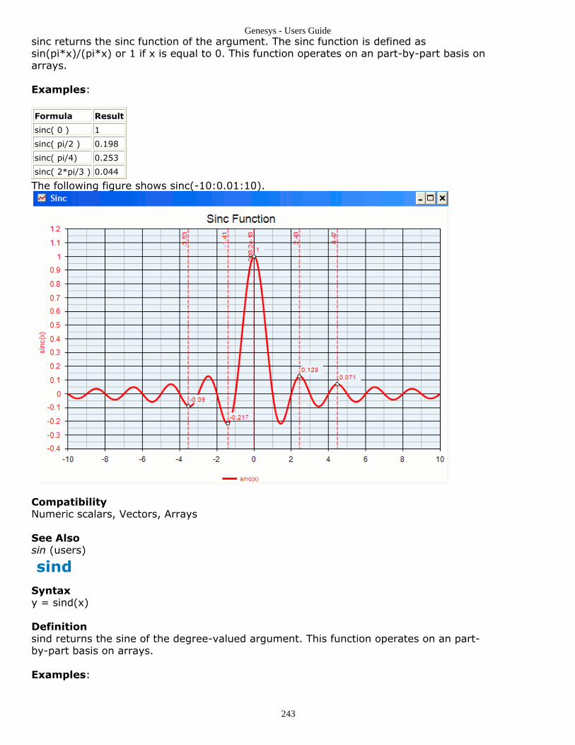
Genesys - Users Guide
243
sinc returns the sinc function of the argument. The sinc function is defined assin(pi*x)/(pi*x) or 1 if x is equal to 0. This function operates on an part-by-part basis onarrays.
Examples:
Formula Result
sinc( 0 ) 1
sinc( pi/2 ) 0.198
sinc( pi/4) 0.253
sinc( 2*pi/3 ) 0.044
The following figure shows sinc(-10:0.01:10).
CompatibilityNumeric scalars, Vectors, Arrays
See Alsosin (users)
sindSyntaxy = sind(x)
Definitionsind returns the sine of the degree-valued argument. This function operates on an part-by-part basis on arrays.
Examples:

Genesys - Users Guide
244
Formula Result
sind( 0 ) 0
sind( 90 ) 1
sind( -90 ) -1
sind( [45 60]) [0.707 0.866]
CompatibilityNumeric scalars, Vectors, Arrays
See Alsoasin (users)sin (users)
sinhSyntaxy = sinh(x)
Definitionsinh returns the hyperbolic sine of the number, or (exp(x) - exp(-x)) / 2. This functionoperates on an part-by-part basis on arrays.
Examples:
Formula Result
sinh( 1 ) 1.175
sinh( 5 ) 74.203
sinh( [pi/3 0] ) [1.249 0]
CompatibilityNumeric scalars, Vectors, Arrays
See Alsoasinh (users)
sizeSyntaxy = size(x)
Definitionsize returns a vector containing the number of parts in each dimension of x. part one of ycorresponds to the number of parts in the first dimension, part two to the seconddimension, and so on.
Examples:
Formula Result
size( [1 2 3 4] ) [1 4]
size( [1 2 3; 4 5 6] ) [2 3]
size( ones(4,3,2) ) [4 3 2]
CompatibilityNumeric Scalars, Vectors, Arrays
skewnessSyntax

Genesys - Users Guide
245
y = skewness(x)y = skewness(x,Flag)y = skewness(x,Flag,iDim)
DefinitionReturns the sample skewness of a vector x. Skewness is the third central moment of Xdivided by the cube of the standard deviation.
If Flag is 0 (default), skewness normalizes by N-1 where N is the sample size. If Flag is 1,skewness normalizes by N.
For matrices, this function operates separately on each column and returns a vector. Formulti-dimensional arrays in general, this function operates on the dimension specified byiDim, or the first non-singleton dimension if iDim is not specified.
Examples:
Formula Result
y = skewness( [ 3 ; 4 ; 8 ; 9 ] ) y = 0
y = skewness( [ 1, 2, -5], 1) y = -0.652
CompatibilityNumeric arrays
See Alsokurtosis (users)std (users)var (users)
sortSyntaxy = sort(x)y = sort(x,dim)[y,index]=sort(x)[y,index]=sort(x,dim)
DefinitionThis function sorts contents of the array x in ascending order along one specific dimensionof the array. When unspecified, the innermost non-singleton dimension is chosen. Thefunction can be required to additionally specify the original indices in the sorted order.
Examples:
In the following example note that b is the column-wise (default dim is 1 for a 2x3 matrix)sorted whereas c and d are sorted row-wise. The index matrix associated with d isinterpreted as follows: if the value k appears at a specific location along row i column j, itmeans that the number now placed (row i,column j) was originally the number at (row i,column k).

Genesys - Users Guide
246
Strings can be sorted alphabetically according to ASCII dictionary if the collection ispresented as cells as shown in the following example. Note that here the string "This" isretained as the first part because large-cap letters occur before small-cap letters in theASCII dictionary.
Compatibility:Real-valued numeric vectors and arrays or strings
splineSyntaxpolynomial = spline(originalIndep,originalDep)ORfittedDependent = spline(originalIndep,originalDep,fittedIndep)
DefinitionThis function performs spline polynomial extraction from a one-dimensional functiondefined as the mapping of an original independent vector onto an original dependentvector. If supplied with a third argument explicitly specifying the independent vector towhich fitting is required, the function returns the fitted dependent vector. If the thirdparameter is not supplied then a structure describing the piece-wise polynomial function isreturned, which may then be used in a call to the ppval(polynomial,fittedIndep) functionto generate the fittedDependent variable.
Examples:In the following example, the original mapping of x and sinc(x) are shown in sparselyspaced blue dots, one dot per unit along the independent axis. When four times as muchgranularity is required, an extended fitting vector xx is introduced. Spline curves producedusing this extended independent vector are compared against the true sinc() function of

Genesys - Users Guide
247
the extended vector. Note how there is substantial match when some variation is presentin the original data, e.g. just one non-zero data point in the original dependent vector. Inregions where there is absolutely no off-axis data in the dependent vector i.e. in the side-lobes, the spline() function is still able to partially recover the existence of the side lobes,if not the full amplitude of each.
CompatibilityReal-valued 1-dimensional vector: originalIndep, fittedIndepReal or complex-valued array: originalDep
sqrtSyntaxy = sqrt(x)
DefinitionThis function returns the square-root of the argument.This function operates on an part-by-part basis on arrays.
Examples:
Formula Result
sqrt( 0 ) 0
sqrt( 4 ) 2
sqrt( 2+3i ) 1.67415+j0.895977
sqrt( -1 ) j
sqrt( [9 16 -4]) [3 4 -2j]
CompatibilityReal and complex-valued scalars, vectors, arrays

Genesys - Users Guide
248
sscanfSyntax:A = sscanf( string, format)A = sscanf( string, format, size)[A, count, msg, next] = sscanf(...)
Definition:Used to read formatted input from a string. Converts the input string using formatargument (format) and puts the results into a matrix (A).
size (optional) argument is used to determine how much data is read. Valid values are:
n read at most n fields from the string
inf read all of the input string
[m,n] read at most m*n fields. Fill a matrix with at most mrows.
count (optional) result is the number of matching fields.msg (optional) is for an error messagenext (optional) is one more than the number of characters match in the input string
Format:
Whitespace characters (space, tab or new lines) are used to delimit fields. Thereare not included in the output.Non-whitespace characters that are not a part of a format specifier are matchedwith the next character in string and then discarded. If the character does not matchsscanf stops process string.Format specifers: %[*][width][modifiers]conversionChar, where:* (optional) match the data in string but do not put the corresponding match in the
output matrix. The format must match but it isn't included in the output.
width (optional) maximum number of characters to match in string
modifiers (optional) For compatibility only. valid values (h, l, L)
conversionChar see table below
Conversion Characters:
Type Qualifying Input
c Single character: Reads the next character. If a width different from 1 is specified, the functionreads width characters and stores them in the successive locations of the array passed asargument. No null character is appended at the end.
d Decimal integer: Number optionally preceeded with a + or - sign.
e,E,f,g,G Floating point: Decimal number containing a decimal point, optionally preceeded by a + or - signand optionally folowed by the e or E character and a decimal number.
o Octal integer.
s String of characters. This will read subsequent characters until a whitespace is found (whitespacecharacters are considered to be blank, newline and tab).
u Unsigned decimal integer.
x,X Hexadecimal integer.
stdSyntaxy = std( x )

Genesys - Users Guide
249
y = std( x, Flag )y = std( x, Flag, iDim )
DefinitionReturns the standard deviation of a vector x.
If Flag is 0 (default), std normalizes by N-1 where N is the sample size. If Flag is 1, stdnormalizes by N.
For matrices, this function operates separately on each column and returns a vector. Formulti-dimensional arrays in general, this function operates on the dimension specified byiDim, or the first non-singleton dimension if iDim is not specified.
Examples:
Formula Result
y = std( [ 3 ; 4 ; 8 ; 9 ] ) y = 2.9439
y = std( [ 1, 2, 3], 1) y = 0.8165
CompatibilityNumeric arrays
See Alsokurtosis (users)var (users)skewness (users)
str2numSyntaxy = str2num('xstring')
DefinitionThis function can convert a single real-valued number from string format to numericformat.When supplied with a string containing preceeding non-numeric characters, other thanwhitespace or tab, the function returns zero.
Examples:
Formula Result
str2num('500') 500
str2num('500')
500
CompatibilityString
See Alsonum2str (users)
strcmpSyntaxout = strcmp(str1, str2)out = strcmp(str, ca)out = strcmp(ca1, ca2)

Genesys - Users Guide
250
Definitionout = strcmp(str1, str2) compares two strings, str1 and str2, and returns true (logical 1)if they are identical. If not, then it returns false (logical 0).
out = strcmp(str, ca) compares str with each string in a cell array. It then returns a logicalarray, out, that contains the corresponding logical values on whether the two strings areidentical.
out = strcmp(ca1, ca2) compares each part in ca1 to the corresponding part in ca2. Itthen returns a character array that is the same size as ca1 and ca2 with the correspondinglogical value on whether the two strings are identical.
This function does not ignore case. To ignore case, use the strcmpi function.
Examples:
Formula Result
out = strcmp('One', 'Two') out = 0
out = strcmp('Yes', {'No', 'Yes'}) out = [0,1]
Compatibilitystring array, cell array
See Alsostrcmpi (users)
strcmpiSyntaxout = strcmpi(str1, str2)out = strcmpi(str, ca)out = strcmpi(ca1, ca2)
Definitionout = strcmpi(str1, str2) compares two strings, str1 and str2, and returns true (logical 1)if they are identical. If not, then it returns false (logical 0).
out = strcmpi(str, ca) compares str with each string in a cell array. It then returns alogical array, out, that contains the corresponding logical values on whether the twostrings are identical.
out = strcmpi(ca1, ca2) compares each part in ca1 to the corresponding part in ca2. Itthen returns a character array that is the same size as ca1 and ca2 with the correspondinglogical value on whether the two strings are identical.
This function ignores case. To take the case into account, use the strcmp function.
Examples:

Genesys - Users Guide
251
Formula Result
out = strcmpi('One', 'Two') out = 0
out = strcmpi('Yes', {'No', 'YES'}) out = [0,1]
Compatibilitystring array, cell array
See Alsostrcmp (users)
strncmpSyntaxout = strncmp(str1, str2, n)out = strncmp(str, ca, n)out = strncmp(ca1, ca2, n)
DefinitionThis function compares the first n characters in str1 and str2 and if they are identical, itreturns true (logical 1). Otherwise, it returns false (logical 0).
The function can also compare a string and each part in a cell array, or the parts in twocell arrays.
This function is case sensitive. To ignore case, use the strncmpi function.
Examples:
Formula Result
out = strncmp('example', 'exam', 4) out = 1;
out = strncmp('test', {'exam', 'testing'},4)
out =[0,1];
Compatibilitystring array, cell array
See Alsostrncmpi (users)
strncmpiSyntaxout = strncmpi(str1, str2, n)out = strncmpi(str, ca, n)out = strncmpi(ca1, ca2, n)
DefinitionThis function compares the first n characters in str1 and str2 and if they are identical, itreturns true (logical 1). Otherwise, it returns false (logical 0).
The function can also compare a string and each part in a cell array, or the parts in twocell arrays.
This function is not case sensitive. To take case into account, use the strncmp function.

Genesys - Users Guide
252
Examples:
Formula Result
out = strncmpi('example', 'EXAM', 4) out = 1;
out = strncmpi('test', {'exam', 'TeStING'},4)
out =[0,1];
Compatibilitystring array, cell array
See Alsostrncmp (users)
structSyntaxy = struct(field1,value1,filed2,value2,....,fieldN,valueN)
DefinitionThis function creates a structure parts of which can be of various types ranging fromstrings through complex cell arrays. Each field is assigned the type of the value whichsucceeds it. If the structure contains more than one cell array, like a matrix, all such cellarrays must be of the same size. Note that fields are always specified as strings.
Examples:In the figure below, observe how records of two people who share the same last name canbe saved to and retrieved from a single structure.
CompatibilityNumeric scalars, Vectors, Arrays
sumSyntaxy = sum(x)y = sum(x,dim)
DefinitionReturns the sum of parts of a vector x.
For matrices, this function operates separately on each column and returns a vector. Formulti-dimensional arrays in general, this function operates on the dimension specified bydim, or the first non-singleton dimension if dim is not specified.
The dim argument is optional and specifies which dimension to operate along. For

Genesys - Users Guide
253
example, if dim is 1, this function operates on each column of the argument. If theargument is omitted, the first non-singleton dimension is chosen as the dimension tooperate along.
Examples:
Formula Result
y = sum( [ 10 , 3 , 5 ] ) y = 18
y = sum( [ 2 ; 9 ; 11 ] ) y = 22
y = sum( [ complex( 3 , 3 ) , complex( 5 , 2 ) ] ) y = 8 + j5
y = sum( [ 3 , 2 , 19 ; 5 , 7 , 1.5 ] ) y = [8, 9, 20.5]
y = sum( [ 3 , 2 , 19 ; 5 , 7 , 1.5 ], 2 ) y = [24; 13.5]
CompatibilityNumeric scalars, Vectors, Arrays
See Alsoprod (users)
svdSyntaxs = svd(X)[U,S,V] = svd(X)[U,S,V] = svd(X, 0)[U,S,V] = svd(X, 'econ')
DefinitionLet X be an m x n matrix and k = min(m,n).
S = svd(X) returns, in the vector S, the singular values (in decreasing order) of the matrixX. S is a column vector of size k.
[U,S,V] = svd(X) produces matrices U, S, and V that form the singular valuedecomposition of X, that is, X = U·S·V', whereU is a unitary m x m matrixS is a diagonal m x n matrix whose primary diagonal parts are the singular values (indecreasing order) of XV is a unitary n x n matrix
[U,S,V] = svd(X, 0) OR [U,S,V] = svd(X, 'econ') produce matrices U, S, and V that formthe 'economical' singular value decomposition of X, that is, X = U·S·V', whereU is an m x k matrix containing only the first k columns of the unitary matrix U returnedby [U,S,V] = svd(X)S is a diagonal k x k matrix whose primary diagonal parts are the singular values (indecreasing order) of XV is an n x k matrix containing only the first k columns of the unitary matrix V returned by[U,S,V] = svd(X)
Examples:
>> X = [ 0.60099 0.766416 0.440156; 0.12712 0.857445 0.130142; 0.94683 0.447486 0.559306 ]
X =
0.60099 0.766416 0.440156
0.12712 0.857445 0.130142
0.94683 0.447486 0.559306

Genesys - Users Guide
254
>> S = svd(X)
S =
1.6967
0.663471
0.0347664
>> [U,S,V]=svd(X)
U =
-0.628061 -0.11714 -0.769297
-0.41523 -0.78565 0.458627
-0.658122 0.607481 0.444796
S =
1.6967 0 0
0 0.663471 0
0 0 0.0347664
V =
-0.620837 0.610289 0.492046
-0.667115 -0.740937 0.0772603
-0.411726 0.280286 -0.867134
>> X = [0.723014 0.179696 -0.861837 0.441228; -0.328791 0.934672 1.68603 0.955427]
X =
0.723014 0.179696 -0.861837 0.441228
-0.328791 0.934672 1.68603 0.955427
>> [U,S,V]=svd(X)
U =
-0.293781 0.955873
0.955873 0.293781
S =
2.25294 0 0 0
0 1.07425 0 0
V =
-0.233779 0.553425 0.721934 -0.343335
0.373129 0.415505 -0.509149 -0.654903
0.827729 -0.305779 0.463201 -0.0825176
0.347831 0.653893 -0.0708765 0.668142
>> [U,S,V]=svd(X,'econ')
U =
-0.293781 0.955873
0.955873 0.293781
S =
2.25294 0
0 1.07425
V =
-0.233779 0.553425
0.373129 0.415505
0.827729 -0.305779
0.347831 0.653893
tanSyntaxy = tan(x)
Definitiontan returns the tangent of the radian-valued argument. This function operates on an part-by-part basis on arrays.
Examples:

Genesys - Users Guide
255
Formula Result
tan( pi ) 0
tan( pi/4 ) 1
tan( -pi/4 ) -1
tan( [5*pi/11 -5*pi/11] ) [6.955 -6.955]
CompatibilityNumeric scalars, Vectors, Arrays
See Alsoatan (users)tand (users)
tandSyntaxy = tand(x)
Definitiontand returns the tangent of the degree-valued argument. This function operates on anpart-by-part basis on arrays.
Examples:
Formula Result
tand( 180 ) 0
tand( 45 ) 1
tand( -45 ) -1
tand( [180 45] ) [0 1]
CompatibilityNumeric scalars, Vectors, Arrays
See Alsoatan (users)tan (users)
tanhSyntaxy = tanh(x)
Definitiontanh returns the hyperbolic tangent of the argument, defined as (exp(x) - 1) / (exp(x) +1). This function operates on an part-by-part basis on arrays.
Examples:
Formula Result
tanh( 1 ) 0.762
tanh( 5 ) 1
tanh( pi/3 ) 0.781
tanh( [pi/6 0] ) [0.48 0]
CompatibilityNumeric scalars, Vectors, Arrays

Genesys - Users Guide
256
See Alsoatanh (users)
tcpipSyntaxt = tcpip( ipAddr, nPort)
Definitiontcpip creates a class object to do tcpip i/o over a lan. ipAddr is a string with the IPAddress in dotted format, and nPort is a port number for the connection. Once created,use fopen, fwrite, fread, fprintf, fscanf, fclose to manipulate the port.
Examples:
Formula Result
t = tcpip( '127.0.0.1', 80) Create an object to connect to the web server on this computer (port 80 on 'this')
CompatibilityTCP/IP connections via LAN. ipAddr is a char array, and nPort is an integer.
tcpip PropertiesModify the way the tcpip link works by setting properties in the created class object. tcpipsupports the following properties
Property Description
LocalHost Local host descriptor
LocalPort Local port descriptor
LocalPortMode Specify automatic local port assignment
ReadAsyncMode Specfiy whether an asynchronous read operation.
RemoteHost The remote host ip address (char array)
RemotePort The remote port # (integer)
Terminator Terminator string, such as 'CR/LF'. ASCII value 0 - 127, or 'CR', 'LF', 'CR/LF', or 'LF/CR'
TransferDelay Specifies whether or not to use Nagle's algorithm.
InputBufferSize Size of the input buffer in bytes.
OutputBufferSize Size of the output buffer in bytes.
Timeout Time to wait before timing out on receive (in seconds, floating point).
ticMeasure performance using stopwatch timer
Syntax:ticstart_time = tic
Definition:Starts a stopwatch timer. The output will be the time in ms since the operating systemstarted.Most commonly used with the function toc to measure the performance time of a set ofstatments.
Examples:t1 = tic<statments>

Genesys - Users Guide
257
t2 = tic<statmets>dt1 = toc(t1) % the time elapsed since the first tic was called (or t1)dt2 = toc(t2) % the time elapsed since the second tic was called (or t2)
Compatibility:output is a double
See Also:toc (users)
tocMeasure performance using stopwatch timer
Syntax:tocdt = tocdt = toc(start_time)
Definition:
toc if there are no input and output, toc will just stop the timer.1.dt = toc if only one output is asked, then dt will become the time elapsed since last2.tic was called.dt = toc(start_time) this call will have the output dt to be the time elapsed since3.start_time, where start_time usually is the output of a tic call (eg. start_time = tic)
Examples:
Ex 1:tic<statments>dt = toc % calculates the time elapsed since tic was used, or the time to run thecode in the <statments>
Ex 2:t1 = tic<statments>t2 = tic<statments>dt1 = toc(t1)dt2 = toc(t2)
Compatibility:doubles
See Also:tic (users)
toeplitzSyntaxtm = toeplitz(x)ORtm = toeplitz(x,y)

Genesys - Users Guide
258
DefinitionThis function returns an m x m Toeplitz matrix based on an m-length vector x or acombination of m-length vectors x and y.
When only a single vector is used, the result is a symmetric, Hermitian matrix as shown inthe Tr1 table below. Note that the vector parts are distributed symmetrically with respectto the principal dialoginal which is occupied by the first part of the input vector.
When two vectors are present, the first part of the first vector populates the principaldiagonal as evidenced in the differences between Tr12 and Tr21. The other parts of thefirst vector populate the lower-triangle whereas those of the second vector populate theupper-triangle of the resultant matrix.
Examples:
unmkppSyntax[breaks,coefs,pieces,oredr,dimension] = unmkpp(pp)
DefinitionThis function extracts, from the supplied piecewise polynomial pp, its break points,coefficients, number of pieces, order, and dimension of target. Create pp using spline orthe spline utility mkpp.Breaks and coefficients are presented as row vectors.
Examples:
pp = mkpp([2 4],[4 6]);
[bks,coefs,l,k,d] = unmkpp(pp)
Result:

Genesys - Users Guide
259
CompatibilityStructure
See Alsospline (users)ppval (users)mkpp (users)
usingSyntaxusing('DatasetName');
DefinitionThis function sets the current context in an equation block to the named dataset. Whenset, you can use the variables within the dataset as if there were defined in the equationblock. This function can be used to context switch between datasets in any postprocessing Equation page.
Examples:If there are two datasets, called "Data1" and "Data2" which both contain a variable called"Var1".Then the way to access these variables without confusion is as follows:
using('Data1');
% Assume "Var1" of "Data1" is [3, 6, 9, 12]
z1=Var1/3;
using('Data2');
% Assume "Var1" of "Data2" is [2, 4, 6]
z2=Var1/2;
The results are:

Genesys - Users Guide
260
z1 = [1, 2, 3, 4]
Z2 = [1, 2, 3]
CompatibilityString
varSyntaxy = var( x )y = var( x, W )y = var( x, W, iDim )
DefinitionReturns the variance of a vector x.
If W is 0 (default), var normalizes by N-1 where N is the sample size. If W is 1, varnormalizes by N. If W is a vector, it is treated as coefficient weights for computing thevariance. In this case, the coefficients of W are scaled so that they sum to unity.
For matrices, this function operates separately on each column and returns a vector. Formulti-dimensional arrays in general, this function operates on the dimension specified byiDim, or the first non-singleton dimension if iDim is not specified.
Examples:
Formula Result
y = var( [ 3 ; 4 ; 8 ; 9 ] ) y = 8.6667
y = var( [ 1, 2, 3], 1) y = 0.6667
y = var( [ 1, 2, 3], [0.7, 0.1, 0.2] ) y = 0.65
CompatibilityNumeric arrays
See Alsokurtosis (users)std (users)skewness (users)
warningSyntaxerror('message')
DefinitionPosts the warning message to the error log and also places the yellow warning symbol onthe menu button.
Examples:
Formula Result
warning( 'out of range') the message "out of range" is posted to the Error Log as a warning

Genesys - Users Guide
261
CompatibilityStrings
See Alsoerror (users)
xcorrSyntaxc = xcorr( x, y, maxlags, 'option' )[ c, lags ] = xcorr( ... )
Definitionxcorr estimates the cross-correlation sequence of a random process. Autocorrelation is aspecial case of cross-correlation.
y, maxlags, and 'option' are optional parameters.
When only x is specified i.e. c = xcorr( x ) then c is the autocorrelation sequence for thevector x.
The various 'options' are:
'biased' - Biased estimate of the cross-correlation function Rxy_biased( m ) = [ 1 /N ] * Rxy( m )'unbiased' - Unbiased estimate of the cross-correlation function Rxy_unbiased( m )= [ 1 / ( N - | m | ) ] * Rxy( m )'coeff' - Normalizes the sequence so the autocorrelations at zero lag are identically1.0.'none' - Use the raw unscaled cross-correlations. This is the default.
maxlags - Limits the autocorrelation lag range to [ -maxlags:maxlags ].

Genesys - Users Guide
262
[ c, lags ] = xcorr( ... ) returns two variables c and lags. lags is a vector of the lagindices at which c was estimated. The ' ... ' represent the x, y, maxlags, 'option'arguments.
Examples:
Formula Result
x = [ 1, 2i, 3]y = [ 4, 5, 6 ]c = xcorr( x, y )
c = [ 6 + i333.1e-18, 5 + i12, 22 + i10, 15 + i8, 12 - i333.1e-18 ]
xorSyntaxy = xor(A, B)
DefinitionThis function performs an exclusive OR operation on arrays A and B.It returns a vector of logical values that are true if only one of the corresponding values inA OR B is nonzero, but not both. Otherwise, the value is false. A and B have to be vectorsor arrays of the same size.
Examples:
A = [0 0 pi eps], B=[0 -2.4, 0, 1]
C = xor(A, B) = [0, 1, 1, 0]
zerosSyntaxy = zeros(m )y = zeros(m, n)y = zeros(m, n, p, ...)y = zeros([m,n,p,...] )y = zeros(m, n, p, ..., class)y = zeros([m,n,p,...], class)
DefinitionThis function returns a m by n by ... array with every part equal to 0. If only oneargument is specified and it is a scalar m, then an m x m matrix is returned. A vector ofdimensions may also be passed in. The optional class argument is a string that specifiesthe data type of the array to return.
Examples:
Formula Result
y = zeros( 3 , 2 ) y = [ 0 , 0 ; 0 , 0 ; 0 , 0 ]
y = zeros( 2 ) y = [ 0 , 0 ; 0 , 0 ]
y = zeros( [5 1] ) y = [ 0 ; 0 ; 0 ; 0 ; 0 ]
See Alsoones (users)eps (users)
Using Engineering Language

Genesys - Users Guide
263
Engineering Language is a simple programming language with structured controlstatements. Variable types are defined in context and matrices and arrays can be easilymanipulated with equations.
Example: here's a simple equation block
x=3
if x==3 then
y = 4*x + cos(z)
else
y = 4*x + sin(z)
endif
In this block we set x to be 3, then if x is 3 we set y to be 4* x +cos( z ).
Recommendation: we recommend you create two separate equation blocks if you have input equations(such as tunable variables) and output equations (such as post-processing). This will generally speed upsimulations and guarantee validity of the input variables even if the output data is messed up.
Equations (in both languages) are case-sensitive. So X=3 and x=3 define two different variables.
Important: You can use a one-line equation in most part parameters and in many other parameter entryfields.
In a part parameter that expects a string (such as substrate) precede the line with an =.For example,
=mysubst
will attempt to parse the mysubst formula and then find the substrate named that. If youhave mysubst defined in an equation somewhere as mysubst="simple", then this will usethe substrate named simple . Similarly, to define a string in parameters that may allowequations, precede the line with a single quote or use double-quotes around the line.
'simple
"simple"
both produce the string "simple".
Note: parameters that expect strings by default draw the string in green.
StatementsAn equation block consists of one or more statements. Statements are separated by linebreaks or semicolons. The following two equation blocks are equivalent:
X = 2
Y = 3
and
X = 2; Y = 3;
Complicated statements can span multiple lines and use control structures like whileloops, for loops, and if statements.

Genesys - Users Guide
264
The following statement types are supported by Engineering equations: assignment,comment, label, goto, if, for, while, function, or return. The format of each statement typeis described below.
Assignments
An assignment statement assigns a value to a variable. The syntax of an assignmentstatement is as follows:
_Variable_Name_ = Expression
For example,
X = 3.6
Y = sin(3*PI)
Z = [1;2;3]
s21 = [My Folder].Linear1_Data.S21
are all assignments.
A variable name must start with a letter or an underscore character, and can containalphanumeric characters and underscore characters. An expression can contain numericaloperations involving numbers, other variables, and function calls.
Vectors and matrices can be defined inline, as the following example illustrates:
x = [1, 2, 3] 'A row vector
y = [1; 2; 3] 'A column vector
z = [1,2,3; 4,5,6] 'A 2x3 matrix
Comments
A comment starts with an apostrophe character (') and continues for the rest of that line.The following are examples of comments:
X = R * cos( theta ) ' here is one comment
' Here is another comment
In the example above, the assignment statement is executed, while both comments areignored.
label statement
A label statement defines a point in the equation block for goto statement destinations.See the goto statement for more details. The syntax of the label statement is:
label _labelname_
goto statement
This statement causes the equation parser to jump to a label defined by a label statementand continue execution from that point. The syntax of the goto statement is:

Genesys - Users Guide
265
goto _labelname_
if statement
The if statement is a control structure that allows one set of statements to execute if acondition is met, and optionally, another set of statements to execute if the condition isnot met. Valid syntax for the if statement is:
if _expression_ then
one_or_more_statements
else
one_or_more_statements
endif
1.
if _expression_ then
one_or_more_statements
endif
2.
if _expression_ then _statement_
3.
If expression evaluates to a nonzero value, the statement block following then isexecuted, otherwise that statement block is skipped. If an else block is specified andexpression evaluates to zero (false), the else block is executed. Expression isgenerally a Boolean expression.
Example:
x = 3
y = 2
if x == y then ' Note that double equals are used for comparison
x = x + 1
y = y - 2
else
x = 0
endif
for statement
The for loop statement is a control structure that allows a set of statements to repeatedlyexecute according to the value of the loop variable. The syntax is as follows:
for _variable_name_ = _expression_ to expression
one-or-more-statements
next
1.
for variable_name = expression to expression step expression
one-or-more-statements
next
2.
A loop variable named variable-name is initialized to the first expression value. Thestatement block following the for loop definition is executed, and the loop variable isincremented by 1 in the first syntax, or by the value of the expression after step inthe second syntax. The statement block repeatedly executes until the loop variableexceeds the value of expression after to. The following example clarifies this:

Genesys - Users Guide
266
x = 0; y = 0
for i = 1 to 5
x = x + 10
y = y + 100
next
After execution completes in the above example, i is equal to 5, x is equal to 50, andy is equal to 500.
while statement
The while loop statement is a control structure that executes a set of statementsrepeatedly based on a condition. The syntax is as follows:
while _expression_
one-or-more-statements
wend
As long as expression evaluates to a nonzero number, the statements execute. Once thelast statement in one-or-more-statements is reached, expression is once again evaluated.When expression evaluates to zero (false), execution continues after wend.
function statement
The function statement is used to define functions or procedures. A function takes zero ormore parameters as input and returns exactly one value as output. All variables usedwithin a function are local; that is, you cannot use variables defined in a function inanother function or in the main equation block. The syntax of the function statement is asfollows:
function _function-name_ ( _param1_ , _param2_ )
one-or-more-statements
end
If the function takes no parameters, the parentheses must still be present after function-name . If the function returns a value, you should use a return statement in the one-or-more-statements block.
The following example is a function used to calculate the inductor value necessary toproduce a resonance at a given resonant frequency and capacitor value:
function ResL(C, F)
' L is in nH, C is in pF, F is in MHz
FHz = 1e6 * F
CFarads = 1e-12 * C
Omega = 2 * PI * FHz
LHenries = 1 / (Omega^2 * CFarads)
return LHenries * 1e9
end
Note: One or more return statements may be present in the function's statement block.
The function defined above may be called as follows:
L = ResL(50, 25.8) ' get me the L value in nH for 50 pF and 25.8 MHz

Genesys - Users Guide
267
return statement
This statement returns a value from a function and exits the function. The format of thereturn statement is:
return expression
The function call then evaluates to the value of expression .
OperatorsOperators and their descriptions are listed in the table below. Examples for each operatorare also listed.
Operator Description Example
+ Addition a + b
.+ Addition (ignores whether operands are swept or not) a .+ b
- Subtraction a - b
.- Subtraction (ignores whether operands are swept or not) a .- b
* Multiplication or Matrix Multiplication a * b
.* part-by-part Matrix Multiplication (ignores whether operandsare swept or not)
a .* b
/ Division a / b
./ part-by-part Division (ignores whether operands are swept ornot)
a ./ b
^ Exponentiation a ^ 2 (means a-squared)
% Modulus a % b
& Boolean And a & b
| Boolean Or a | b
~ Boolean Not ~a
= Assignment Operator a = 2
== Boolean Comparison a == b
> Boolean Greater Than a > b
>= Boolean Greater Than or Equal a >= b
< Boolean Less Than a < b
<= Boolean Less Than or Equal a <= b
<> Boolean Not Equal a <> b
@ Returns indices for which var = operand , F@50 returns indicesat which F=50, F@[50,100]
Returns indices at which F isbetween 50 and 100.
Vectors, Matrices, and Multidimensional ArraysEngineering Language allows you to create vectors, matrices, and multi-dimensionalarrays. Vectors and matrices are arrays of 1 and 2 dimensions, respectively. Arrays aredesigned to work with numeric data, including complex numbers. Vectors and matricesmay be defined inline, or may be defined and sized explicitly with the vector, matrix, andarray functions. Here is an example equation block that defines several vectors andmatrices, as well as a multi-dimensional array.
x = vector(3) 'x is a column vector of 3 parts, all zero. The datatype is Complex.
y = matrix(4, 3) 'y is a 4x3 matrix with all parts zero. The datatype is Complex.

Genesys - Users Guide
268
z = array(3, 4, 4, 2) 'z is a 3x4x4x2 array. The datatype is Complex.
a = [1; 2; 3] 'a is a column vector containing the parts 1, 2, and 3
b = [2.5, 3, 8] 'b is a row vector containing the parts 2.5, 3, and 8
M = [1,2,3; 4,5,6; 7,8,9] 'M is a 3x3 matrix with the first row containing 1, 2, and 3.
M = ["hello"; "goodbye"; "Hi"] 'M is a 3-part string array
Note that semicolon denotes the end of a row, while comma separates row parts. Theexception to this is string arrays which are always 1-dimensional arrays, regardless ofwhether semicolons or commas are used to separate the parts when defining the array.
Indexing into Arrays
An part in an array variable is accessed with the following syntax:
var[index1, index2, ..., indexN]
where var is the name of the array, and var is an array of dimension N. The first part in adimension has index 1. A colon may be used to indicate every part in thedimension. If the leading dimensions correspond to independent values (eg. the Smatrix produced by Linear Analysis, which has the first dimension correspond to theindependent value of F, a frequency vector) then these dimensions may be omitted, and acolon is assumed for these dimensions.
The following example illustrates indexing into arrays.
M = [1,2,3; 4,5,6; 7,8,9] 'M is a 3x3 matrix with the first row containing 1, 2, and 3.
a = M[2,1] ' a equals 4
b = M[1,:] ' b is the row vector [1,2,3]
c = M[:,[1;3]] ' c is the 3x2 matrix [1,7; 2,8; 3,9]
M[1,1] = 5 ' the part in the first row and first column of M is now 5
Note that only scalar assignment is supported when assigning a value into an part in anarray.
Vectors may also be used for specifying multiple parts in a dimension. The followingexample illustrates this:
M = [1,2,3; 4,5,6; 7,8,9]
a = M[ [1; 3], [1; 2] ] ' a is the matrix [1,2; 7,8]
Searching Vectors and Indexing into Sweeps
Sometimes it is useful to know at what index or indices in an array a particular value iscontained. To find what indices a vector contains a certain value or range of values, the@ operator may be used. This is especially useful for indexing into sweeps to extractdesired data. A single number following the @ operator searches a vector for that singlenumber. If a two-part vector follows the @ operator, the two numbers are treated as arange. The following example illustrates the use of the @ operator:
F = [100; 200; 300; 400; 500; 600]
i = F@300 ' i equals 3
n = F@[200,350] ' n is the vector [2;3]
X = F[n] ' X is the vector [200;300]

Genesys - Users Guide
269
Suppose S is an S-matrix produced by linear analysis of a 2 port network. S contains datafor 10 frequencies: 10 MHz through 100 MHz in steps of 10 MHz. That is, S has anindependent value F, the frequency vector, of length 10. Therefore, S is a 10x2x2 array. The following example shows how to extract the S21 parameter at frequencies 30 - 50MHz:
s_21 = S[F@[30,50], 2, 1]
Suppose we have a sweep that produced a swept variable PPORT which contains thepower at ports. This variable is contained in a dataset called HB1_Data and has twoindependent variables because both frequency and input power were swept. Let us saythat the frequency variable is Freq while the input power variable is called Pin. Supposewe wanted to extract the trace where the frequency is 2000 MHz and the power is sweptfrom -15 to -11 dBm. We can make use of the intersect function to find the indices ofPPORT corresponding to this trace as follows:
using("HB1_Data")
indices = intersect( Freq@2000, Pin@[-15,-11] )
trace = PPORT[indices] ' trace contains the desired values of output power
String arrays may be searched in the same manner, but no ranges are allowed for strings:
strings = ["hello", "goodbye", "Hi"]
i = strings@"Hi" ' i equals 3
j = strings@"hi" ' i equals 0, since the string "hi" is not found in the array.
Range Vectors
A range defines a column vector in either of the following two ways:
start:stop
start:stepsize:stop
where start, stepsize, and stop are expressions. If stepsize is left out, it is assumed to be1. A range creates a column vector with the first part value being equal to start , eachsuccessive part being stepsize greater than the previous part, until stop is reached. Ranges may also be used to index into arrays and extract desired sub-arrays. Thefollowing example illustrates the use of ranges.
x = 1:10 'x is the column vector [1;2;3;4;5;6;7;8;9;10]
y = 1:2:10 'y is the column vector [1;3;5;7;9]
M = [1,2,3; 4,5,6; 7,8,9] ' M is a 3x3 matrix with the first row containing 1, 2, and 3.
a = M[1:2, 2:3] ' a is the 2x2 matrix: [2,3; 5,6]
b = M[1:2:3, :] ' b is the 2x3 matrix: [1,2,3; 7,8,9]
Mathematical Operations on Arrays
Mathematical operations on arrays are supported. In general, any scalar operation orfunction may be performed on an array, and the operation will be performed on an part-by-part basis, producing a resulting array that has the same dimensions as the originalarray. The following example illustrates this:
x = [1,2; 3,4]

Genesys - Users Guide
270
y = [1,1; 1,1]
z = x + y 'z is the matrix [2,3; 4,5]
z = z - 1 'z is now the matrix [1,2; 3,4]
w = sin(z) 'w is the matrix [sin(1), sin(2); sin(3),sin(4)]
Multiplication is a special-case operator. When using the multiplication operator on amatrix or vector, matrix-multiplication is assumed. To do an part-by-part multiplication,the .* operator is used. Here is an example:
x = [1,2; 3,4]
y = [1;1]
z = x * y 'z is the vector [3;7]
w = x .* [1,0;0,1] 'w is the same matrix as x
To find out the dimensions of an array, use the size function. To find out how many partsare in an array, use the prod function to calculate the product of the parts of the vectorreturned by the size function:
x = [ 1,2,3; 4,5,6]
x_dims = size(x) 'x_dims is the vector \[2;3\]
num_parts = prod(x_dims) 'num_parts is 6
Shortcuts, and FunctionsThe following are built-in variables and functions that you can use in any equation block.
Variables
FREQ - Frequency variable (in Hertz) set by the frequency-domain simulatorsTIME - Time variable (in Seconds) set by the time-domain simulatorTEMPERATURE - Temperature (in Celsius) set by simulatorsPI - Constant equal to 3.1415926535897932
Shortcuts
SUB_ER substrateer(SUBST) (compatibility with 2004 which used mm for units)SUB_TAND substratetand(SUBST) (compatibility with 2004 which used mm for units)SUB_RHO substraterho(SUBST) (compatibility with 2004 which used mm for units)SUB_TMET (1000*substratetmet(SUBST)) (compatibility with 2004 which used mmfor units)SUB_ROUGH (1000*substraterough(SUBST)) (compatibility with 2004 which usedmm for units)SUB_H (1000*substrateh(SUBST)) (compatibility with 2004 which used mm forunits)SNM where N and M are digits S[N,M] (index into S-parameters)YPNM where N and M are digits YP[N,M] (index into Y-parameters. YP will be createdand set to stoy(YP, ZPORT))
Measurement FunctionsMeasurement functions are typically used when looking at the output of linear simulations.Remember that all measurement data is in MKS fundamental units, so these functions useMKS input and produce MKS output. S21, for example, is not in dB.

Genesys - Users Guide
271
sm_gamma1( S ), sm_gamma2( S )
Returns simultaneous match gamma ( reflection coefficient into port 1 or 2 ) for 2-port Sparameters. Shortcut:
GMi sm_gammai( S )
sm_y1( S ), sm_y2( S )
Returns simultaneous match input admittance ( into port 1 or 2 ) for 2-port S parameters.Shortcut:
YMi sm_yi( S )
sm_z1( S ), sm_z2( S )
Returns simultaneous match input impedance ( into port 1 or 2 ) for 2-port S parameters.Shortcut:
ZMi sm_zzi( S )
stab_fact( S )
Returns stability factor ( K ) from 2-port S parameters. Shortcut:
K stab_fact( S )
stab_meas( S )
Returns stability measure( B1 ) from 2-port S parameters. Shortcut:
B1 stab_meas ( S )
stoh( s, zport )
Converts 2-port S parameters to H parameters.
stoy( s, zport )
Converts S parameters to Y parameters. Shortcut:
YP stoy( S,ZPORT )
stoz( s, zport )
Converts S parameters to Z parameters. Shortcut:
ZP stoz( S,ZPORT )
voltage_gain( s, zport, i, j )

Genesys - Users Guide
272
Returns port-to-port voltage gain from i to j. Shortcut:
Eij voltage_gain( S,ZPORT,i,j )
vswr( s )
Returns the vswr of an S-parameter. Shortcuts:
VSWR vswr( diag( S ) ) 'returns a vector of all port VSWR value
VSWRi vswr( s[i,i] ) 'VSWR at port _i _
y toz( Y )
Converts Y parameters to Z parameters.
zin( s, zport ), yin( s, zport )
Returns the input impedance or admittance looking into a port. Parameters are S andZport. Shortcuts:
ZIN zin( diag( S ),ZPORT ) 'returns a vector of all input impedances
YIN yin( diag( S ),ZPORT ) 'returns a vector of all input admittances
ZINi zin( S[i,i],ZPORT[i] ) 'returns input impedance at port i
YINi yin( S[i,i],ZPORT[i] ) 'returns input admittance at port _i _
Variables in Datasets and other EquationsIt is possible to refer to a variable that is located inside a dataset or an equation by usingthe dot operator (.) to specify the path of the variable in the workspace tree. If the objectin the workspace tree that contains the desired variable does not have an alphanumericname (eg. it contains spaces), then the name of the object must be surrounded by squarebrackets or braces. The following example illustrates the use of the dot operator:
X = Linear1_Data.S ' The S variable in dataset Linear1_Data is copied to X
Y = [Equation set 1].x ' Y equals the variable x defined in an equation block named "Equation
set 1"
Z = {Equation set 1}.x ' same as Y
A graph series may refer to variables in the same manner. For example, entering thefollowing measurement as a graph series is valid:
Linear1_Data.S21
Units of Measure
Data that comes from a dataset (simulation) will always be in MKS. So, for example,

Genesys - Users Guide
273
PPORT (power at a port) is in Watts. F (linear analysis frequency vector) is in Hz, T (Time)is in seconds. When you use this data in an equation, manipulate the MKS data. When youview the data in a graph or table you can see the table with a display unit of measure.
Example:
PPORT[2,2] - fundamental power at port 2 is stored in Watts but displayed in dBm
F[12] - 12th frequency is stored in Hz but displayed in MHz
To have an equation variable use a unit of measure, use the setunits function. So
F = [100e6;110e6]
setunits("F","MHz")
will create a two part vector at 100 and 110 MHz. Doing the setunits both identifies thetype of data (time, here) and the desired (time) unit to display in (MHz). When you wantto contrast measured and calculated results, remember to create your data in MKS.
Swept Arrays
A Swept Array is an array variable with an independent variable link. Typically,simulations create swept variables when they run. In Linear Analysis, S is a swept variableand the independent variable (link) is the F variable. When we plot S the X dimension isFrequency and the X coordinates are the values of the F array (the Y coordinates areusually dB(Sxx)).
Swept variables are used in equations differently from non-swept variables. With a sweptvariable the first dimension (the swept dimension) is often elided (left out) and thevariable is treated like many variables with shape equal to the non-swept shape. Also,when swept variables are plotted the swept dimension (variable) is used for the X axis.
Example: in a transient analysis (CAYENNE simulator) of a 2-port device we have a VPORTvector of size Tx2 where T is the size of the time (T) vector. If we assume we have 100times then T is of size 100x2 and we can do...
VPORT[2] - the Port_2 voltage array swept over time (size 100x1)
VPORT[1,2] - the first voltage at port 2 (scalar)
[1,2]*VPORT - produce a swept array of size 100x1 where each value is VPORT [f,1] + 2 *VPORT[f,2]
treating VPORT as a bunch of 2 part vectors
Note that in this example both VPORT[2] and VPORT[1,2] are valid constructs because VPORT is swept.
To create a swept variable in equations, use the setindep function. This assigns an arrayas the independent vector for a second array.
Example: to create a swept voltage array
V = 1:100 ' create a vector of length 100 consisting of the numbers 1 through 100.
T = 1e-9*(1:100) ' and again, except scaled by 1e-9
setunits("T","ns") ' set T to ns(time)

Genesys - Users Guide
274
setunits("V","mV") ' set V to mV(voltage)
setindep("V","T") ' say the voltage was swept by time
Example: if we want to contrast transient voltage with voltage squared (for some reason)
Vout = mydata.VPORT[2] ' get the output port voltage from mydata
Vsq = Vout .* Vout ' part-by-part mult. (Square each part)
setindep("Vsq","mydata.T") ' use the same indep as VPORT so we can graph it
Using Math LanguageMath Language, along with most of its built-in functions, was designed to be compatiblewith m-file script syntax.
StatementsAn equation block consists of one or more statements. Multiple statements placed on thesame line are separated by line breaks, commas, or semicolons. The following twoequation blocks are equivalent:
X = 2Y = 3
and
X = 2, Y = 3
If you end a statement with a semicolon, it does not generate output in the commandwindow.
Complicated statements can span multiple lines and use control structures like whileloops, for loops, and if statements.
The following statement types are supported by Mathematics Language equations:assignment, comment, label, goto, if, for, while, function, or return. The format of eachstatement type is described below.
Assignments
An assignment statement assigns a value to a variable. The syntax of an assignmentstatement is as follows:
variableName = Expression
For example,
X = 3.6;
Y = sin(3*PI);
Z = [1 2 3];
are all assignments.
A variable name must start with a letter, and can contain alphanumeric characters andunderscore characters. An expression can contain numerical operations involvingnumbers, other variables, and function calls.

Genesys - Users Guide
275
Vectors and matrices can be defined inline, as the following example illustrates:
x = [1 2 3] % a row vector
y = [1;2;3] % a column vector
z = [1 2 3; 4 5 6] % a 2x3 matrix
Tune Assignments
A Tune Assignments assigns a variable a specific value while marking it as Tunable. Atunable variable can then be tuned from the Tune Window and can be used byevaluations, such as Sweeps, that operate on tunable variables.
When a Tunable variable is tuned from the Tune Window, the resultant value is thenupdated in the Equation block where it was originally defined.
The syntax for a Tune Assignment is as follows, where Constant represents a real-valuedconstant:
variableName = ?Constant
For example:
x = ?23 % x is tunable with initial value 23
y = ?-1.5 % y is tunable with initial value -1.5
Comments
A comment starts with a percent character (%) and continues for the rest of that line. Thefollowing are examples of comments:
X = R * cos( theta ) % Here is an in-line comment
% Here is another comment
In the example above, only the assignment statement is executed, while both commentsare ignored.
if statement
The if statement is a control structure that allows one set of statements to execute if acondition is met, and optionally, another set of statements to execute if the condition isnot met. Valid syntax for the if statement is:
if _expression_
_one_or_more_statements_
elseif
_one_or_more_statements_
else
_one_or_more_statements_
end
1.
if _expression_
_one_or_more_statements_
end
2.
3.

Genesys - Users Guide
276
if _expression_, _statement,_ end
If expression evaluates to a nonzero value, the following statement block is executed,otherwise that statement block is skipped. If an else block is specified and expressionevaluates to zero (false), the else block is executed. The expression is generallyBoolean in construction.
Example:
x = 3
y = 2
if x == y % Note that double equals are used for comparison
x = x + 1
y = y - 2
else
x = 0
end
for statement
The for loop statement is a control structure that allows a set of statements to repeatedlyexecute according to the value of the loopVariable. The syntax is as follows:
for _loopVariable_ = _startValue_ : _stepValue_ : _stopValue_
_one_or_more_statements_
end
The loopVariable is initialized to the startValue. When stepValue is explicitly mentioned,loopVariable increments by it until it reaches or exceeds the stopValue. When leftunspecified, stepValue is assumed to be of unit magnitude. The following example clarifiesthis:
x = 0, y = 0
for i = 1 : 5 % i, the _loopVariable_ takes the values [1 2 3 4 5]
x = x + 10
y = y + 100
end
After execution completes in the above example, i is equal to 5, x is equal to 50, and y isequal to 500.
while statement
The while loop statement is a control structure that executes a set of statementsrepeatedly based on a condition. The loop is exited when the condition is no longersatisfied. The syntax is as follows:
while _expression_
_one_or_more_statements_
end
As long as expression evaluates to a nonzero number or a Boolean true, the statementsexecute repeatedly. When expression evaluates to zero (false), execution continues afterend. The following example clarifies this:

Genesys - Users Guide
277
x = 1, y = 15;
while ( y )
x = x * y;
y = y - 1;
end
After execution completes, when y reaches 0 in the above example, x equals factorial ofthe original value of y.
function statement
The function statement is used to define functions or procedures. A function takes zero ormore parameters as input and returns exactly list of values as the result. All variablesused within a function are local; that is, you cannot use variables defined in a function inanother function or in the main equation block. However, you can use variables defined inthe equation block in the function. The syntax of the function statement is as follows:
function <resultList> = functionName( <paramList> )
_computation_statements_
_calls_to_other_functions_
end % Note: this end is optional
If the function takes no parameters, the parentheses must still be present afterfunctionName . If the function returns a value, you should set the values in the<resultList> block.
<paramList> and <resultList> are lists of variable names separated by commas. If thelast variable in <paramList> is 'varargin', then the function can take in an unspecifiednumber of arguments, and the remaining arguments are placed into the 'varargin' cellarray which can be accessed from within the function. Similarly, if the last variable in<resultlist> is 'varargout', then the function can return an unspecified number of returnvalues which are set in the function by assigning to the 'varargout' cell array.
Inside a function definition, you may use the variables named 'nargin' and 'nargout' whichhold the number of arguments passed in to the function and the number of return valuesrequested by the caller, respectively. These may be used for error checking or otherpurposes.
The following example is a function used to calculate the inductor value necessary toproduce a resonance at a given resonant frequency and capacitor value:
function resonantInductor = ResL( resonantCapacitor, resonanceFrequency )
% inductance is in nH, capacitance is in pF, frequency is in MHz
FHz = 1e6 * resonanceFrequency;
CFarads = 1e-12 * resonantCapacitor;
Omega = 2 * pi * FHz;
LHenries = 1 / (Omega^2 * CFarads);
resonantInductor = LHenries * 1e9; % the return value
end
The function defined above may be called as follows:
L = ResL(50, 25.8) % computes the L value in nH resonanct with 50 pF at 25.8 MHz
You may return multiple values by listing them in the result expression, as in

Genesys - Users Guide
278
function [Ind, Q] = ResL( C, F, R )
Ind = 1
Q = 2
end
this is used as [MyInd, MyQ] = Resl(a,b,c)
The following example illustrates a function that takes in a variable number of argumentsand returns a variable number of results.
function varargout = f(varargin)
SumOfArgs = 0;
for i = 1 : nargin
SumOfArgs = SumOfArgs + varargin{i}
end
varargout{1} = SumOfArgs
if nargout > 1
varargout{2} = 2 * SumOfArgs
end
end
Suppose we call this function as follows:
[a, b, c] = f(1, 2, 3, 4)
a would be set to 10 (the sum of the input arguments), b would be set to 20, and c wouldbe blank since it was not assigned to in the function.
OperatorsOperators and their descriptions are listed in the table below. Examples for each operatorare also listed.

Genesys - Users Guide
279
Operator Description Example
+ Addition a + b
- Subtraction a - b
* Matrix Multiplication a * b
.* part-by-part Matrix Multiplication a .* b
/ Matrix Right-Division a / b
./ part-by-part Division a ./ b
\ Matrix Left-Division a \ b
.\ part-by-part Left-Division a .\ b
^ Matrix Exponentiation a ^ 2 (means a-squared)
.^ part-by-part Exponentiation a .^ b
' Matrix conjugate-transpose (hermitian) a'
.' Matrix transpose (no conjugation) a.'
& part-wise Boolean And a & b
&& Boolean And a && b
| part-wise Boolean Or a | b
|| Boolean Or a || b
~ Boolean Not ~a
= Assignment Operator a = 2
== Boolean Comparison a == b
> Boolean Greater Than a > b
>= Boolean Greater Than or Equal a >= b
< Boolean Less Than a < b
<= Boolean Less Than or Equal a <= b
~= Boolean Not Equal a ~= b
Vectors, Matrices, and Multidimensional ArraysMathematics Language supports vectors, matrices, and multidimensional arrays. Columnvectors are treated as Nx1 matrices, while row vectors are 1xN matrices. Vectors andmatrices can be defined inline using bracket notation, as shown below.
a = [1;2;3] % a is a column vector containing the parts 1, 2, and 3
b = [2.5 3 8] % b is a row vector containing the parts 2.5, 3, and 8
c = [1, 2, 3] % c is a row vector containing 1, 2, and 3. Commas are optional
M = [1 2 3; 4 5 6; 7 8 9] % M is a 3x3 matrix with the first row containing 1, 2, and 3.
M = ['help1'; 'help2'; 'help3'] % M is a 3 by 5 character array
M = ['help1' 'help2' 'help3'] % M is the string 'help1help2help3'
Note that semicolon denotes the end of a row, while comma separates row parts.
Indexing into Numeric Arrays
An part in an array variable is accessed with the following syntax:
_matrixVariable_(index1, index2, ..., indexN)
where matrixVariable is the name of the N-dimensional array. A colon may be used to indicate every part in the dimension. If only one indexingdimension is specified, then the array is linearly indexed, which means that the array is

Genesys - Users Guide
280
treated as a flat list (in column-wise order) and the N'th part of the list is returned.
Note: If only one indexing dimension is specified and it is a colon, then the array is returned as a singlecolumn vector with N parts, where N is equal to the number of parts in the array.
The following example illustrates indexing into arrays.
M = [1 2 3; 4 5 6; 7 8 9] % M is a 3x3 matrix with the first row containing 1, 2, and 3.
a = M(2,1) % a equals 4
b = M(1,:) % b is the row vector [1,2,3]
c = M(:,[1;3]) % c is the 3x2 matrix formed by taking the columns of the 1st and 3rd columns of
all the rows [1,3; 4,6; 7,9]
d = M(:) % d is the column vector [1;4;7;2;5;8;3;6;9]
e = M(6) % e equals 8 because it is the 6th part when M is traversed column-by column
M(1,1) = 5 % sets the value of the part in the first row and first column of M to 5
Vectors may also be used for specifying multiple parts in a dimension. The followingexample illustrates this:
M = [1,2,3; 4,5,6; 7,8,9]
a = M( [1; 3], [1; 2] ) % a is the matrix [1,2; 7,8]
Multi-dimensional arrays are formed by combining arrays of smaller dimensions in nestedfashion using [s and semi-colons. For instance, a three dimensional array of size 3x2x2would have two levels of []s:
M3D = [ [1, 2, 3; 4, 5, 6]; [-1, -2, -3; -4, -5, -6] ]
Searching Vectors and Indexing into Sweeps
The example named Indexing Sweeps with Math Lang.wsx located in the Examples\Equations folder walksthrough the material discussed in this section.
Sometimes it is useful to know at what index or indices in an array a particular value iscontained. To find what indices a vector contains a certain value or range of values, thefind function may be used. This is especially useful for indexing into sweeps to extractdesired data. The following example illustrates a simple case using the find function:
F = [100; 200; 300; 400; 500; 600]
i = find(F == 300) % i equals 3
n = find(F >= 200 & F <= 350) % n is the vector [2, 3]
X = F(n) % X is the vector [200;300]
Suppose V1 is a waveform of voltages as a function of time. V1 contains data for 101timepoints: 0 ns through 100 ns in steps of 1 ns. That is, V1 has an independent value T,the time vector, of length 101. Therefore, V1 is a 101x1 array. The following exampleshows how to extract a subset of the voltage waveform and construct a new timeindependent variables corresponding to that subset:
% Suppose V1 and T already exist, as described above
time_indices = find(T >= 10e-9 & T <= 20e-9); % indices where T is between 10 and 20 ns
V1_subset = V1(time_indices); % extract waveform between 10 and 20 ns
time_subset = T(time_indices); % ditto for the time indep
setindep('V1_subset', 'time_subset'); % now if we plot V1_subset, we see a nice x-axis

Genesys - Users Guide
281
We can use the same approach for indexing into multi-dimensional sweeps. The key is touse the find function to extract the correct indices.
Indexed Assignments
Mathematics Language supports assigning a value or values into arrays. If you assign datato parts outside the current dimensions of an array, the array is automatically re-sized toaccommodate the new data, while any new parts in the array are initialized to zero.
When assigning from one array to another in the form A = B, the following rules must beobeyed:
The number of subscripts specified for array B not including trailing 1's may notexceed the number of dimensions of BThe number of non-scalar subscripts specified for A is equal to the number of non-scalar subscripts specified for BThe length and order of all non-scalar subscripts specified for A is equal to the lengthand order of all non-scalar subscripts specified for B
The following code example illustrates various aspects of indexed assignments.Initially the variable x does not exist.:
x(2,3) = 5; % x is created to be a 2x3 matrix with the entry at (2,3) equal to 5 and the other
parts equal to zero so x is [0, 0, 0; 0, 0, 5]
x(:,2) = [11; 22] % x is now [0, 11, 0; 0, 22, 5]
x(1, [1 3]) = [100 200] % x is now [100, 11, 200; 0, 22, 5]
x(1:6) = 1:6 % x is now equal to [1 3 5; 2 4 6]
x(1,1,2) = 23 % now x is a 2x3x2 array with x(1,1,2) equal to 23
Range Vectors
A range defines a row vector in either of the following two ways:
start:stop
start:stepsize:stop
where start, stepsize, and stop are expressions. If stepsize is left out, it is assumed to be1. A range creates a row vector with the first part value being equal to start , eachsuccessive part being stepsize greater than the previous part, until stop is reached. Ranges may also be used to index into arrays and extract desired sub-arrays. Thefollowing example illustrates the use of ranges.
x = 1:10 % x is the row vector [1 2 3 4 5 6 7 8 9 10]
y = 1:2:10 % y is the row vector [1 3 5 7 9]
M = [1 2 3; 4 5 6; 7 8 9] % M is a 3x3 matrix with the first row containing 1, 2, and 3.
a = M(1:2, 2:3) % a is the 2x2 matrix: [2,3; 5,6]
b = M(1:2:3, :) % b is the 2x3 matrix: [1,2,3; 7,8,9]
Mathematical Operations on Arrays
Mathematical operations on arrays are supported. In general, any scalar operation orfunction may be performed on an array, and the operation will be performed on an part-by-part basis, producing a resulting array that has the same dimensions as the originalarray. The following example illustrates this:

Genesys - Users Guide
282
x = [1,2; 3,4]
y = [1,1; 1,1]
z = x + y % z is the matrix [2 3; 4 5]
z = z - 1 % z is now the matrix [1 2; 3 4]
w = sin(z) % w is the matrix [sin(1), sin(2); sin(3),sin(4)]
Multiplication is a special-case operator. When using the multiplication operator on amatrix or vector, matrix-multiplication is assumed. To do an part-by-part multiplication,the .* operator is used. Here is an example:
x = [1 2; 3 4]
y = [1;1]
z = x * y %z is the vector [3; 7]
w = x .* [1 0;0 1] % w is the same matrix as x
To find out the dimensions of an array, use the size function. To find out how many partsare in an array, use the length function:
x = [1 2 3; 4 5 6]
x_dims = size(x) % x_dims is the vector [2 3]
num_parts = length(x) % num_parts is 6
Cell ArraysCell arrays are arrays that support each part having a differing data type. Each part in acell array is called a cell. As an example, you may have a 1x3 cell array in which the firstcell is a number, the second cell is a character array, and the third cell is a structure.Furthermore, parts of cell arrays may be cell arrays themselves. Cell arrays, just likenumeric arrays, may have any number of dimensions. Cell array vectors and matricesmay be defined inline as shown here:
X = { [1 2; 3 4] 'abc' 3j } % X is a 1x3 cell array containing a 2x2 real matrix, a 1x3 character
array, and a complex scalar
Y = { {1 2}; {1 2; 3 4} } % Y is a 2x1 cell array containing a 1x2 cell array and a 2x2 cell array
Indexing into Cell Arrays
There are two ways to index into a cell array, described here:
M{indices} % returns the contents of the cell at the index specified by indices
M(indices) % returns the cell or cells at the index or indices specified by indices
Numeric arrays contained in cell arrays may be indexed inline as well:
M{2,3}(6) % returns 6th part of the array contained in the cell array M at location (2,3)
M{2,3}{2}(6) % returns 6th part of the array contained in the 2nd part of the cell array located
in the cell array M at location (2,3)
The following example illustrates indexing into cell arrays.
M = { 1 'abcd' [2j 56; 3 j] {6 7} } % M is now a 1x4 cell array
a = M{1} % a equals 1

Genesys - Users Guide
283
b = M{2} % b equals the 1x4 character array 'abcd'
c = M(2) % c equals a 1x1 cell array that contains 1 part: a 1x4 character array 'abcd'
d = M{3}(1,1) % d equals 2j
e = M{4} % e equals the cell array {6 7}
StructuresA structure is a data type with named fields. Each field has a name and a value. The valuemay be of any type, including a cell array or another structure. Structure arrays of anynumber of dimensions are supported. In a structure array, all structures in the array havethe same field names.
Structures may be defined inline as shown here:
x.field1 = 23; % x is a structure with a field named "field1" with value 23
x.hello = {1 2}; % x now has another field named "hello" whose value is a 1x2 cell array
x(3).hello = 1; % x is now a 1x3 structure array with fields "field1" and "hello". The third
part's hello field has value 1.
You may use the fieldnames function to determine what field names are in a structure.fieldnames returns a cell array of strings.
Structures may also be built using the struct function.
Network Communication and Instrument ControlThe Math Language includes TCP/IP communication capabilities. This enables control ofinstruments.
When you create an equation set to do communication you will almost always want it tobe not Auto-Calc. It should only calculate when specifically requested, otherwise everytime an input variable changes it will rerun. It will also run on load. Turn off auto-calc byclicking the Check-Calculator tool button when viewing the equation set.
TCP/IP communication is done via the tcpip class, which is constructed using the tcpipfunction. A simple example follows (waitfor is a wait-for-character routine, PSAip containsthe IP address string of an instrument, while PSASpciPort contains the port number to usefor communications):
% - set up the tcpip pipe to the instrument
t = tcpip(PSAip, PSASpciPort) % build tcpip object using the PSA ip address and spci port
t.Terminator = 'CR/LF'; % set Terminator field
t.InputBufferSize = 100000; % use a big buffer
% - open the port
fopen(t)
% - set real data format
fprintf(t, 'form:data real,64')
% - swap byte order
fprintf(t, 'form:border swap')
% - read the trace
fprintf(t, 'trace? trace1') % tell it to send the first trace
a3 = waitfor(t, '#') % the # is followed by some count chars
% - get the # of count bytes
aBytecnt = fread( t, 1, 'uchar=>ushort')
tTotal = str2num( aBytecnt)
% - if valid # count bytes, read them
if tTotal > 0 && tTotal < 7 % we will never have more than 6 digits of stuff
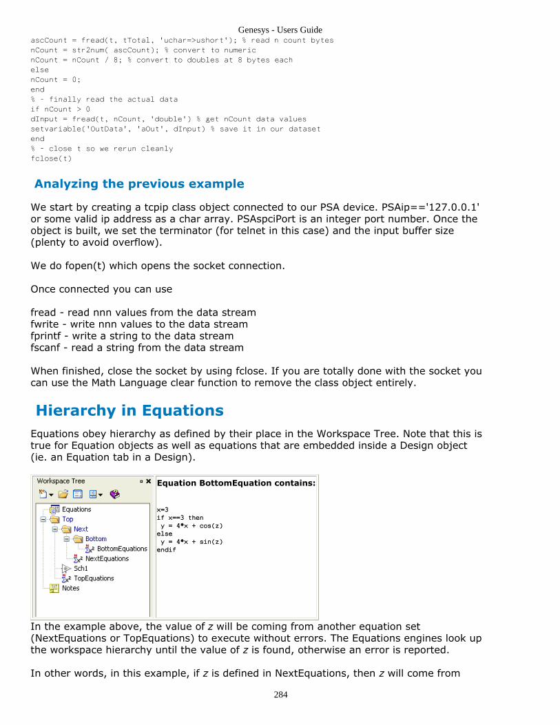
Genesys - Users Guide
284
ascCount = fread(t, tTotal, 'uchar=>ushort'); % read n count bytes
nCount = str2num( ascCount); % convert to numeric
nCount = nCount / 8; % convert to doubles at 8 bytes each
else
nCount = 0;
end
% - finally read the actual data
if nCount > 0
dInput = fread(t, nCount, 'double') % get nCount data values
setvariable('OutData', 'aOut', dInput) % save it in our dataset
end
% - close t so we rerun cleanly
fclose(t)
Analyzing the previous example
We start by creating a tcpip class object connected to our PSA device. PSAip=='127.0.0.1'or some valid ip address as a char array. PSAspciPort is an integer port number. Once theobject is built, we set the terminator (for telnet in this case) and the input buffer size(plenty to avoid overflow).
We do fopen(t) which opens the socket connection.
Once connected you can use
fread - read nnn values from the data streamfwrite - write nnn values to the data streamfprintf - write a string to the data streamfscanf - read a string from the data stream
When finished, close the socket by using fclose. If you are totally done with the socket youcan use the Math Language clear function to remove the class object entirely.
Hierarchy in EquationsEquations obey hierarchy as defined by their place in the Workspace Tree. Note that this istrue for Equation objects as well as equations that are embedded inside a Design object(ie. an Equation tab in a Design).
Equation BottomEquation contains:
x=3
if x==3 then
y = 4*x + cos(z)
else
y = 4*x + sin(z)
endif
In the example above, the value of z will be coming from another equation set(NextEquations or TopEquations) to execute without errors. The Equations engines look upthe workspace hierarchy until the value of z is found, otherwise an error is reported.
In other words, in this example, if z is defined in NextEquations, then z will come from

Genesys - Users Guide
285
there. If NextEquations does not define z then the Equations engine looks up anotherfolder level to TopEquations for z .\
Equations on the same level of hierarchy should all be visible to each other.
Design-time vs. Run-time hierarchy
The above discussion of hierarchy is called design-time hierarchy, because while you arenot simulating, the workspace tree defines the scoping of variables. However, when yourun a simulation, the situation can be different.
Suppose, for example, that we have 2 designs as shown in the below picture. Bothdesigns have an Equation tab (and possibly a Parameters tab, which is equivalent, sinceParameters get passed into the design's Equations at run-time).
In the situation shown in the above picture, when you are NOT running a simulation (ie.you are in design-time), the design called SubNetwork will be able to see variables thatare defined in the Equations tab of the design called TopLevel, simply becauseSubNetwork is located in a folder beneath the level of hierarchy that TopLevel is in.However, suppose that, as shown, SubNetwork defines a subnetwork model. Also supposethat the schematic in TopLevel defines an instance of SubNetwork (ie. it has a part thatreferences the SubNetwork model). When you run a simulation (ie. during run-time), aModel hierarchy is defined in which SubNetwork is a child of TopLevel, since an instance ofa SubNetwork model is instantiated inside of TopLevel. Because of this, SubNetwork cansee all of TopLevel's variables. This is what makes the passing of parameters fromTopLevel to SubNetwork possible.
It is important to note that when you are editing a design (ie. you are in design-time), thevalues of parameters you see in your design are those calculated using the design-timehierarchy. For example, if you define a Design that contains Parameters, and you use oneof those parameters inside your Design, you will see the value of that parametercorrespond to the "Default" value of the Parameter that you defined in the Parameterstab. This is, of course, not necessarily the value that will be seen at run-time when yourun a simulation, since that depends on the run-time hierarchy defined by the topology ofthe network you are simulating.
Automatic CalculationIf an Equation object is set to Auto-Calculate, the equations are always kept up to datewhenever a value is requested from them. This is desirable when the equation blockdefines variables that you use in part parameters on a schematic: when you change thesevalues, you want the part parameters that use them to update. However, sometimesthis is undesirable. If, for example, you are using an Equation block to import data froma file or to transfer data to and from an instrument, you do not want the Equations tocalculate unless you specifically tell them to. In these cases, you should disable Auto-Calculate. The Auto-Calculate toolbar button located on the Equation Toolbar (users)toggles automatic calculation on and off.

Genesys - Users Guide
286
There are some cases where you probably want to DISABLE automatic recalculation of an equation block:equations which do file I/O or TCP/IP communications, equations which run simulations via the runanalysisfunction, equations that do time-consuming processing.
If you disable Automatic Calculation , the only way to recalculate the equation is manuallywith the calculate button, or with the F5 or Ctrl+G keyboard shortcuts. Equations thathave Automatic Calculation turned off will not update during simulations. As mentionedbefore, you would normally disable Automatic Calculation for Math Language equationsthat control hardware, for example, so the hardware doesn't get re-controlled every timea variable changes.
If you disable Auto-Calculate in an equation that is a function definition, the function won't exist until youmanually calculate the equation.
Debugging EquationsA fully featured and intuitive debugger is built-in to the equation editing user interface.
Using Breakpoints and Single-Stepping
You can use the Equation Toolbar (users) or its associated keyboard shortcuts in theequation script editor to set breakpoints and to step through your code one line at a time.Breakpoints can be set both in equations contained in the workspace and in a model'sequations (eg. sub-circuits). In all cases, evaluation of equations will be halted when abreakpoint is hit. The user may then execute statements line by line using single-stepping,abort execution, or continue execution until the next breakpoint is hit.
Workspace Equations: to run the equations click the Go button in the EquationToolbar (users). If a workspace equation is set to Auto-Calculate, they will calculatewhenever something they are dependent on triggers a calculation. If any breakpointsare set, the evaluation of the equations is halted and the user interface is brought tothe front, clearly marking what line of code the equation processor is currently haltedat.
It is important to keep in mind that an equation block may be calculated may times due tovarious factors, such as a simulator changing a variable. The evaluation of the equationswill halt whenever the breakpoint is hit. Typical scenarios include:
Equations in sub-circuit models: the breakpoint will be hit once per run of thesimulator except when the equation is dependent on the simulator independentvariable. For example, in the linear simulator, frequency dependent equations willcalculate at each frequency. For CAYENNE (time domain), time dependent equationswill calculate at each T.Equations in a Math Language block: the breakpoint will be hit at each 'tic' of thesimulator as data is delivered to the block.
Setting Breakpoints
Click the Breakpoint Margin at the line you wish to set a breakpoint at in the script editor

Genesys - Users Guide
287
window to toggle a breakpoint on/off. A red dot will appear when the breakpoint is on. TheBreakpoint margin is located between the Line Number and Folding margins. You may alsoset a breakpoint at the current line by using the Ctrl+B keyboard shortcut or clicking theAdd/Remove Breakpoint toolbar button.
When the equation processor hits a breakpoint, the current line it is halted at will display ayellow arrow in the breakpoint margin as can be seen in the picture below. At this pointyou may single-step, step-into functions, continue, or abort execution. If you step-into afunction, a green arrow marks the line that the function was called from.
Using Debug Print functions
The debug print functions shown below produce lines of debug text in the Equation Debugdocking window.Please note that debug lines will only appear in the window after the simulator runs, dueto current multi-threading locks.
Equation Debug docking window
The Equation Debug docking window can be shown/hidden using the Edit/View/DockingWindows/Equation Debug menu path or using the show/hide dockers button on the maintoolbar. This window has a list of debug lines that your equations generate using functionsdescribed below. A sample Equation Debug Window is shown here.

Genesys - Users Guide
288
Debug Functions
There are two functions available (in both Engineering Language and MathematicsLanguage) for writing to the Equation Debug docking window. Both functions add lines tothe Equation Debug Docking Window so you can trace progress as the program runs. Thecode samples are written in Mathematics Language.
dbg_print( 'Message' )
dbg_print( 'Message', 'Equation')
dbg_print( 'Message', 'Equation', Line)
1.
prints the Message in the Equation Debug window. The Equation and Line parametersmay be omitted, in which case the equation engine will attempt to auto-detect whichequation set and line number called the function.
dbg_showvar( 'Message', Variable)
prints Message=VariableValue in formatted output
Tips for Effective Equation WritingAs a program becomes more complex, it becomes necessary to carefully debug and testthe results. Breakpoints and Debug-Print functions can be very helpful, as has alreadybeen discussed. In general, however, there are several things one should get accustomedto doing when writing equations. Below are some tips to follow when an equation iscausing difficulty:
Make sure the input and output equations are in separate blocks1.It is a bad idea to have something like:c = ?4 ' value of some capacitor in the schematics21 = Linear1_Data.S[2,1] ' s21 from analyzing the schematicThe "c" is an input to a schematic; it MUST exist before Linear1_Data is ever created,so this equation block will not compile reliably. Any equation statements that callvariables from analysis datasets should be in a separate block.Let each line compile cleanly before typing more text2.Avoid the temptation to write a long set of statements before verifying that it works;type one line at a time and check that there are no error messages, and that thevariables are showing up in the left side of the equation editor.
Before writing a large loop or in-line vector statement, check the boundary3.valuesInstead of writing a large loop then wondering why there are out of bounds errors orwrong calculations, first type something like:testA = myVector[firstIndex]testB = myVector[lastIndex]

Genesys - Users Guide
289
The values will display in the Variable view; this way you first verify that the initialand final values are as expected; then you can let the loop or vector operation runwith more confidence.Don't try to pack everything into one line of code4.It is very difficult to find the problem when there are too many calculations packedinto a one line statement. By breaking up a line into several variables and lines yougive yourself the chance to debug and find problems, rather than just look at a hugeline that doesn't work as intended.Check dimensions of variables carefully5.Always pay attention to the size and dimension of variables being used; a commonpitfall is to use incorrect multiplication or division of vectors and thus accidentallycreate wrong-sized matrices or other unwanted results.
Careless use of the "/" operator causes a 1601x1601 matrix to be created; thevariables view alerts the user of the problem, so part-wise division can be usedinstead:
Note that the functions numcols( myMatrix) and numrows( myMatrix) can be used to find thedimensions of a variable. For matrix operations, the number of columns of a left-hand operatorshould equal the number of rows of a right-hand operator, while for part-wise operations thedimensions should be identical.
Use the Command Window to output or change variable values6.See Equations User Interface for more information about the Command Window.Use the online help7.The online help for equations is extensive. You can select a keyword in the equationeditor and press F1 for context help on that keyword. General equation help is in theUser's Guide manual Using Equations section.
Equations User InterfaceThe following image shows a typical Equations window:

Genesys - Users Guide
290
The Equations window has three subwindows:
The Variable Viewer, located on the left.The Script Editor, located on the upper right.The Command Window, located on the lower right.
The Equations window also has an associated toolbar, see Equation Toolbar (users).
Among the simplest application of equations is to define a variable in the Script Editor area (upper right),such as myvar=123 (then press "Go")Then myvar can be entered into component properties on the schematic, to drive component values.Entering myvar=?123 (ie. adding the question mark) makes the value myvar tunable in the tune window.After pressing "Go", the variable value should appear in the Variable Viewer (left side). If nothing appearsin the Variable Viewer after pressing "Go", this usually indicates some problem with equation syntax.Typically the error messages window will provide some clues.
Variable Viewer
The Variable Viewer displays any variables that currently exist in the Equations object. Ifthe variable is a scalar, the value is displayed. If the variable is an array, the type anddimensions of the array are displayed.
If you right-click on any variable displayed in the Variable Viewer, you will be presentedwith a menu containing options to plot the variable on a graph or display it in a table. Ifyou wish to see the variable's value without creating a table, you can do so in theCommand Window, as discussed below.
The following buttons are located at the top of the Variable Viewer window: EquationLanguage, Units, and Go.
The Equation Language button allows you to set the language of the Equations to bedefined, as shown here:
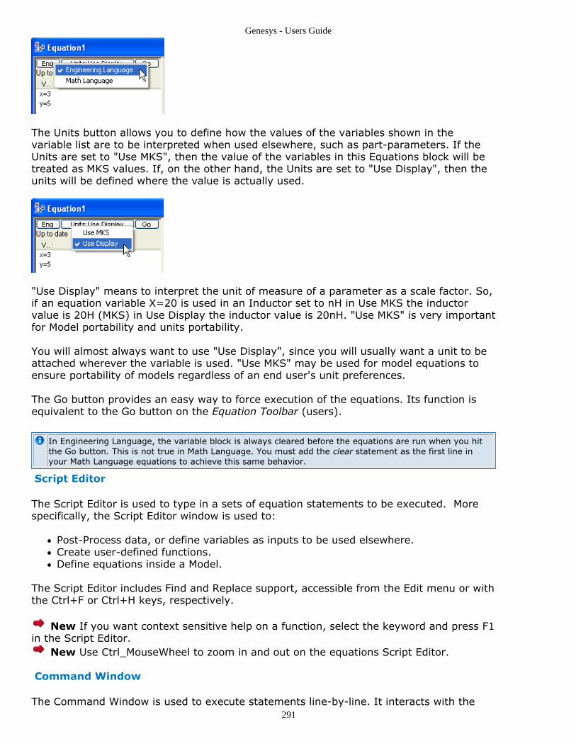
Genesys - Users Guide
291
The Units button allows you to define how the values of the variables shown in thevariable list are to be interpreted when used elsewhere, such as part-parameters. If theUnits are set to "Use MKS", then the value of the variables in this Equations block will betreated as MKS values. If, on the other hand, the Units are set to "Use Display", then theunits will be defined where the value is actually used.
"Use Display" means to interpret the unit of measure of a parameter as a scale factor. So,if an equation variable X=20 is used in an Inductor set to nH in Use MKS the inductorvalue is 20H (MKS) in Use Display the inductor value is 20nH. "Use MKS" is very importantfor Model portability and units portability.
You will almost always want to use "Use Display", since you will usually want a unit to beattached wherever the variable is used. "Use MKS" may be used for model equations toensure portability of models regardless of an end user's unit preferences.
The Go button provides an easy way to force execution of the equations. Its function isequivalent to the Go button on the Equation Toolbar (users).
In Engineering Language, the variable block is always cleared before the equations are run when you hitthe Go button. This is not true in Math Language. You must add the clear statement as the first line inyour Math Language equations to achieve this same behavior.
Script Editor
The Script Editor is used to type in a sets of equation statements to be executed. Morespecifically, the Script Editor window is used to:
Post-Process data, or define variables as inputs to be used elsewhere.Create user-defined functions.Define equations inside a Model.
The Script Editor includes Find and Replace support, accessible from the Edit menu or withthe Ctrl+F or Ctrl+H keys, respectively.
New If you want context sensitive help on a function, select the keyword and press F1in the Script Editor.
New Use Ctrl_MouseWheel to zoom in and out on the equations Script Editor.
Command Window
The Command Window is used to execute statements line-by-line. It interacts with the

Genesys - Users Guide
292
same variables that are visible to the Script Editor. It is a useful debugging tool since thecontents of a variable can be displayed here.
If an assignment statement does not end in a semicolon, the results of that assignmentare outputted in the Command Window, as can be seen in the above figure. If anassignment statement does end in a semicolon, then the dump of the contents of theresult is suppressed.
Any errors or warnings caused by executing a line in the Command Window are outputtedto the Command Window.

Genesys - Users Guide
293
Examining DatasetsDatasets are containers which hold data, such as the results of a simulation or a table ofinput. The results are stored in Variables which can be viewed in tabular form within thedataset, plotted on a graph, displayed in an output Table, etc. Examine a dataset byopening it with a double-click. You can also add new variables to a dataset (for sweepingor just for analizing the data in greater detail).
Open the Linear Simulation Template (via the Start Page). On Linear1_Data, click thevariable "S" on the left-side of the window, to see its values. Hovering the mouse over avariable pops up some info, which varies according to the measurement.
In the display above the left-hand pane shows all of the result variables (including F, thefrequency or independent variable). The right-hand pane shows whatever piece of datayou have selected in the left pane. The upper left-corner box in the grid is the units ofmeasure (MHz down and dB for the values). The lower right pane (which is usuallycollapsed – drag the divider bar upwards to see it) displays a summary of the variableinformation.
Each type of analysis creates a different dataset with differing variables which aredetermined by the Analysis. Often, the variable is directly associated with a particularmeasurement. Linear analysis (as seen above) creates data with F (frequency), S, ZPORT(port impedance) and CS (noise correlation matrix).
Each dataset contains variables, which can be matrices, vectors, or scalars. Thesevariables are either automatically created by simulation runs or manually by the user.Note that when a dataset is created by a simulation, the data within that dataset is alwaysin MKS. You may display the data in a unit of your choice, but the actual data values areMKS values.
Click S on the left to show the tabular display of values in the grid on the top-right. Itshows that the frequencies analyzed were 100, 109, 118, ..., 1000 MHz. The S-Parameters are shown in columns. The single grid-cell (top left corner of the grid) whichsays MHz:dB shows that the units for Frequency are MHz and the data values are shown

Genesys - Users Guide
294
in dB. The display on the bottom-right (which is usually collapsed) shows the type andsize of the clicked data.
In addition to seeing the simulation results, Datasets can have short equations to help youanalyze and diagnose issues with your circuits. For details, see Creating Variables (users).
ContentsCreating Datasets (users)Creating Variables (users)Using Dataset Variables (users)Importing Variables (users)Variable Properties (users)
Creating DatasetsDatasets are usually created automatically when Analyses run. Some analyses(particularly SPECTRASYS) can create more than one dataset. Within the dataset are thefundamental results – measurements created by the simulation.
In addition, a blank dataset can be created manually from the workspace tree (in thedocking window) via the "new item" button (although that is rarely neccesary).
The actual data within a dataset is determined the Analyses settings. CAYENNE andHARBEC and SPECTRASYS all let you limit which data is created during the simulation run.This can reduce the size of datasets significantly and also reduce their complexity.
To examine a dataset, open it by double-clicking it in the workspace tree.
Here's a minimal SPECTRASYS dataset:
If we rerun SPECTRASYS with all of the output options enabled, we get this:

Genesys - Users Guide
295
Now we can't even fit the entire dataset contents in the window.
Although more complex and intimidating there are many cases where more data is betterthan less. However, file storage requirements go way up with this sort of data.
Creating Variables
Variable Properties Dialog Box
For complete description of Variable Properties dialog box, see Variable Properties(users)
Why add variables to a dataset?
Add a variable to examine more closely a piece of data (such as ang(S[2,1]) to1.examine S21's angle). Don't forget that all measurement data is fundamentally inMKS units.Add a variable to propagate it during a sweep (enable the propagate option in the2.sweep and it will sweep the variable along with the rest of the measurement data).Add a variable to use in an optimization.3.
How to add a variable to a dataset
Open Linear Simulation Template / Linear1_Data, as described above.1.Right-click the white area on the left and select Add New Variable...2.
Add a variable named Var1.3.Type ang(S[2,1]) for the formula.4.Leave the Independent Variable field blank; it will be automatically filled in based on5.the indep associated with the "S" variable.Optionally, you can choose a display option for the dataset view of the variable. If the

Genesys - Users Guide
296
6.variable type is integer or floating point, select a display unit; if it's complex, select acomplex number formatting option.Click OK.7.
To get...8.
For most formulas, the Unit of Measure and Independent Variable will fill themselves9.in once the formula is parsed.
How to delete a variable from a dataset
Right-click the variable and select Delete
Importing VariablesVariables can be imported to the dataset from any text file. Access this feature by right-clicking in the variable block of the data set and choosing "Import Variable".

Genesys - Users Guide
297
Browse and select a file. Enable "First Column is Independent Data" if the first column ofthe data is independent data (swept). Name the variable in the Variable Name field.
The data should be formatted as a list or matrix of numbers. Semicolons (" ; ") andspaces (" ") are used to indicate breaks between values Other characters are treated aszeroes. Begin the data with !Units unitindep unitdep to define a unit of measure for thedata. Other rows that begin with a ! are ignored as comments.
Example (Choose Real, check First column as independent)

Genesys - Users Guide
298
Importing Complex Variables
Complex data can be imported in several formats. A typical usage is shown below, wherethe independent vector is frequency (MHz) and the dependent is S21 in DB and ANGformat. The same conventions apply here as for reals; spaces, tabs, and semicolons definebreaks between entries.

Genesys - Users Guide
299
Example using rectangular coordinates (Re + Im)
Notes
Complex data should come in pairs of columns; two parts are needed to specify a1.point in the 1D complex space. A warning is given if there is an odd number ofcolumns (excluding the independent vector).To use the dB scale for complex numbers, the unit should be specified as dB;2.otherwise the absolute scale is used based on whatever unit is defined. For example,input impedance should have a unit of "Ohm" which can also potentially have aphase; thus it cannot be in Ohms and dB simultaneously.Typical units: dB, dBm, dB10, dB20, Abs, Ohms, V, A, mil, pF, nH3.The independent variable must be real ( this will typically correspond to time or4.frequency, both of which are real quantities).
Using Dataset VariablesYou can create variables and analyses will create variables when they run.
To graph a Dataset variable

Genesys - Users Guide
300
Right-click the variable and see creating a graph from a dataset (users).
To duplicate a Dataset variable
Right-click the variable and select Duplicate
To edit a Dataset variable
You can not edit Measurement variables (variables created during a simulation run).You can edit variables you create. Double-click the variable or right-click it and selectProperties from the menu.
To delete a Dataset variable
You should not delete Measurement variables (variables created during a simulationrun). You may delete variables you create. Right-click it and select Delete from themenu.
To view a Dataset variable
If the variable is an array, click it and the right pane will fill with the array values. Ifthe variable is a scalar the value should be shown in the list on the left.
To export a Dataset variable
Right-click the variable and select Export. This will export it into an XML data form.
Using DatasetsDatasets are extremely useful for comparing different circuit configurations. You can run asimulation, save the data, then change some parameters, rerun the simulation andcompare the two sets of data easily.
Normally, an analysis has the dataset name stored within it. You might set that name to aformula based on the parameters, but it's simpler to just Snapshot or Checkpoint thedataset.
To Checkpoint a Dataset
Right-click the dataset and select Snapshot. Another dataset named mydata_Snap iscreated. This Snap dataset contains the numerical data from the first dataset (allformulas are parsed and converted to data and the formula text is stored in the variabledescription).

Genesys - Users Guide
301
To compare PPORT[2] for the two datasets just enter two measurements in a graph ortable like this:
The HB1_Data_Snap.VPORT entry says to use the VPORT variable from HB1_Data_Snap.
Note we use db() here because the data in the dataset is in MKS and we want dBV fordisplay.

Genesys - Users Guide
302
Variable PropertiesThis window defines a variable and its display properties:
Name – The variable name.The name must start with a letter and contain only letters, numbers, and/or theunderscore "_" character.Names are case-sensitive. (V1 is a different variable than v1.)
Formula – The equation which defines the variable's value.The Engineering Language or Math Language equation may refer to othervariables, functions, define vectors, matrices, etc. Please see the appropriatesection in the User's Guide for details on using Equations.
Independant Variable – One or more associated variables, which define relateddata, such as the X-Axis variable (which is the first indep).
If there is more than one independant variable, each indep should be separatedby a vertical-bar character "|".
Description – The discription of the variable, usage notes, etc.Complext Format – If the value is one or more complex numbers, the values can bedisplayed in several formats:
Default – Allows Genesys to automatically determine the most appropriateformat to use.Real + Imaginary – Displays the values using real and imaginary values.Magnitude + Angle – Displays the values using magnitude and angle. Themagnitude is displayed using the units specified in the "Display Magnitude In"dropdown. The angle is displayed using the global Angle units, as specified inTools / Options.Magnitude Only – Only the magnitude is displayed.
Units Of Measure – The units used for displaying the variable in the DataSet viewwindow.Display Magnitude In – If the value is a complex number and the Complex Formatincludes magnitude, this specifies the units to use (for magnitude).

Genesys - Users Guide
303
GraphsGraphs display data from datasets (users) or equations (users), which are usuallymeasurement data derived from the analysis of a design. For more information on menuitems, refer Graph Menu (users) or Graph Toolbar (users) in the Appendix sections.
ContentsTypes of Graphs (users)Creating Graphs (users)Graph Properties (users)Graph Series Wizard (users)Using Markers on Graphs (users)Annotating Graphs (users)Zooming Graphs (users)Measurement Wizard (users)
Types of GraphsGenesys has several types of graphs, including:
Rectangular Graphs - a Cartesian coordinate plot.3D Graphs - can display a measurement versus frequency versus a parametersweep.Antenna Plots - displays Far Field measurements.Polar Charts - displays complex data, such as S-Parameters or impedances.Smith Charts - similar to a Polar Chart, displays impedance and/or admittance.
In addition, data can be displayed in a spreadsheet-style Table (users) view. Thesediffering output options allow you to display data in a variety of formats.
Rectangular GraphsA rectangular graph is a Cartesian coordinate plot. You can use a rectangular graph todisplay two-dimensional data versus frequency (for example: magnitude or phase of acomplex measurement, but not both).
In the figure below, the S-parameter insertion loss and return loss of a bandpass filter areplotted. There are 3 types of markers shown: a peak marker, a regular (fixed frequency)marker, and a valley marker. You can add to any rectangular graph. Regular markers canalso be placed on circular charts.

Genesys - Users Guide
304
If you do not like the small circles, squares, or triangles that show each data point, hide them using theShow Symbols On Trace option on the Graph menu.
3D GraphsA 3D graph is used to display a measurement versus frequency versus a parametersweep. You can sweep any tunable parameter or variable. In the figure below, the gain ofa 5th-order Butterworth bandpass filter is displayed from 62.5 to 87.5 MHz while 2capacitors are varied (swept).
A 3D graph requires a parameter sweep to generate three-dimensionaldata.

Genesys - Users Guide
305
3D graphs cannot display markers. However, you can plot a sweep on a rectangular graphif you need markers. Here's the same sweep:
Antenna Plots
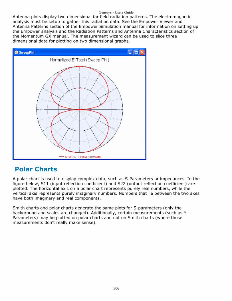
Genesys - Users Guide
306
Antenna plots display two dimensional far field radiation patterns. The electromagneticanalysis must be setup to gather this radiation data. See the Empower Viewer andAntenna Patterns section of the Empower Simulation manual for information on setting upthe Empower analysis and the Radiation Patterns and Antenna Characteristics section ofthe Momentum GX manual. The measurement wizard can be used to slice threedimensional data for plotting on two dimensional graphs.
Polar ChartsA polar chart is used to display complex data, such as S-Parameters or impedances. In thefigure below, S11 (input reflection coefficient) and S22 (output reflection coefficient) areplotted. The horizontal axis on a polar chart represents purely real numbers, while thevertical axis represents purely imaginary numbers. Numbers that lie between the two axeshave both imaginary and real components.
Smith charts and polar charts generate the same plots for S-parameters (only thebackground and scales are changed). Additionally, certain measurements (such as YParameters) may be plotted on polar charts and not on Smith charts (where thosemeasurements don't really make sense).

Genesys - Users Guide
307
Smith ChartsA Smith chart is used to display complex data, such as S-Parameters or impedance. In thefigure below, S11 (input reflection coefficient) is plotted on a Smith chart. The horizontalaxis on a Smith chart represents real numbers from zero (0) to infinity, and numbers offthe horizontal axis represent numbers having a nonzero imaginary part.Smith charts inGenesys have two grid options:
ImpedanceAdmittance
You can enable or disable both grids using the Smith Chart Properties window.

Genesys - Users Guide
308
Smith charts can plot special circular measurements, like gain, noise, and stability circles.When displaying one of these measurements, place one or more makers to set a locus forthe measurement circles.
Creating GraphsGraphs can be created manually, however the easier way to provide a context first. Seesections on creating a graph from a dataset or creating a graph from a schematic.
The easiest way to add an arbitrary measurement to an existing graph is via theMeasurement Wizard (users).
Manually create a graph
Click the New Item button ( ) on the Workspace Tree toolbar.1.Select Graphs.2.Click on the graph type, e.g click on menu item Add Rectangular Graph...3.A property page for that graph type will pop-up.4.Click on the Graph Properties tab.5.Add the measurement you want to plot.6.Click OK.7.
Create a graph from a dataset
Right click a variable in a dataset. Select Add Graph... and click on New Graph.

Genesys - Users Guide
309
Create a graph from a schematic
Right-click a port or node on a schematic and select Add New Graph/Table then1.the measurement you want to graph from the menu.
The actual items available on the menu are context-sensitive, based on the part or node you clickedand the simulations available. For example, the Relevant S-Parameters option generatesmeasurements for all S-parameter measurements that are pertinent to the indicated port. Also, theworkspace must contain at least one analysis referring to this schematic design to make this featureavailable. (Otherwise there is nothing to plot.)
To create another graph, right click the port again and select a different option. Your2.screen should now have a spectrum similar to this:

Genesys - Users Guide
310
Double-click a graph to change the graph's properties. Right-click a trace or legend to3.make specific changes to the appearance of the trace or legend. Hover over a symbol(a dot on the trace) to get a pop-up showing the value at that point. Check out theGraphs tutorial video for tips and techniques.
Graph PropertiesGraph properties define a graph object. The Graph Properties window permits changesto properties such as the title or a series, i.e. a plot of a measurement variable.
Changing Graph Properties
The Graph Properties window initially appears when a graph is created, so that you canadd a series and/or customize the graph. You can make additional changes after the graphis created by right clicking the graph window or double clicking an "empty" area of thegraph window and then selecting Graph Properties... as illustrated below.

Genesys - Users Guide
311
Graph Properties Dialog
The following Graph Properties window was created for a General plot type with aRectangular graph format and plots two variables from two different datasets.
Name – The name of the graph object, which is shown on the workspace treeGraph Title – The plot title, which is drawn at the top of the graph (like a heading)

Genesys - Users Guide
312
Show All Columns – When this box is checked, infrequently-used columns in theSeries window (such as On Right and Hide?) are shown.Advanced... Button – Clicking this button displays the Advanced GraphProperties dialog, as described below.
Series Settings
The following series window has defined two series for plotting.
Edit/Add Button – Clicking on the Edit or Add buttons will pop-up the Graph SeriesWizard (users) for a series definition.Remove Button – Clicking on this button removes the associated series.Context – The text provides context for the Variable text box. If left blank, theVariable text box must have a fully qualified variable name. Typically, the context isthe dataset name where the variable is defined. To graph an equation variable, setthis text box to [Equations]. The equation hierarchy is searched for the equationvariable. If the equation variable is not found, an error is logged.Variable – The text contains the name of the variable that is to be graphed.Label (Optional) – The text contains the axis label for the series. If left blank, theVariable text is used.On Right / On Bottom – If the box is checked, the an alternate vertical axis for theseries is placed on the right side of a rectangular graph. Polar charts use On Bottomto indicate the use of the "lower" radial axis.Hide? – If the box is checked, the series is not plotted.Color Button – Click on this button to change the color that has been assigned tothe series.Type – This informational (read only) text box states the series plot type.
Note: Checkpoint traces are NOT shown in the series grid. You can remove all the checkpoint traces on agraph by clicking the Checkpoint button on the Graph Toolbar (users). You can change the trace colorby right-clicking a trace.
Axis Settings Tabs
The lower portion of the window contains various axis and settings tabs, which depend onthe graph type.
The following is an example of a rectangular graph with a single vertical axis.
If both vertical axes are used, the Y-Axis tab name is changed to Left Y-Axis, and anadditional tab labeled Right Y-Axis is added. Most of the settings are similar.
Auto-Scale – When checked, the axis automatically sets its limits to match the

Genesys - Users Guide
313
range of the data which is being plottedLabel – Use this label to customize the axis nameLogarithmic – When checked, the axis is drawn with a logarithmic scaleMin – Sets the lower numerical range of an axisMax – Sets the upper numerical range of an axisUnits – Sets the units-of-measure used by the axis (and Min and Max)# Divisions – Sets the number of divisions to use on the axis; contains Auto if thedivisions will be determined automatically
Tip: To control the axis tick marks, you can set the Min and Max fields to appropriate numbers, e.g. inthe above examples you might want to specify the Max to 1000e-6 s.
Similarly, an Antenna plot has Angle Axis and Top Radial Axis, and a 3D chart has X,Y, and Z-Axis, but the individual settings are otherwise identical.
For a polar plot, there is simply a tab labeled Polar.
Upper and Lower Scale – Polar charts have both an upper and lower scale, so thatdifferent numerical ranges may be compared on the same plot.Linear or dB – Indicates which scaling method to useMaximum – Typically 0.0 for dB and 1.0 for Linear
Likewise, a Smith chart has a Smith tab, with appropriate settings.

Genesys - Users Guide
314
Show Impedance Grid – When checked, this option enables the impedancebackground "graph paper" (default ON, drawn in black)Show Admittance Grid – Enables the admittance background "graph paper"(default OFF, drawn in dark red)Show Normalized Impedances – Normally checked: The graph will use normalizedimpedances (range will be converted from 0.0 - Reference Impedance to 0.0 - 1.0);when unchecked, the graph will be drawn using the full numerical range of the dataReference Impedance – Allows user to change the labels shown on the Smith chartif desired. Note that the Reference Impedance entry is only active if the "shownormalized impedances" box is NOT checked. The default is 50 Ohms, although 75often used for certain applications (like cable TV).Grid Density – Sets grid spacing
Automatic – Determines appropriate grid spacing (ultra fine to very coarse)and optionally draws text labelsFine – Has text labels and uses fine grid spacingCoarse – No text labels with widely spaced grid
Note: The Reference Impedance entry does not affect the position of traces on the Smith chart – itonly affects the labels (for user convenience in reading the chart). For instance, it is possible to have aschematic with 2 different ports, port1 having Zo=50 and port2 having Zo=100. Then S11 and S22 couldsimultaneously be displayed on a Smith chart. The center value of the Smith chart is dependent on theport impedance from which a given measurement is derived.
General Tab
The General tab contains generalized graph settings, such as a description field.
Description – An optional description which is saved with your graph

Genesys - Users Guide
315
Goals Tab
If the appropriate check boxes are filled, matching optimization or yield targets for allmeasurements can be displayed as a goal line or as a goal area.
Goal Lines – Specifies the thickness of the goal line(s): Thin, Medium, Thick, Heavy,or NoneGoal Fill – Sets the transparency of the shaded goal area: Invisible, Faint, Semi-Transparent (Normal), or HeavyShow Optimization targets – Enables Optimization target drawing. (Shows targetsset up in separate Optimization evaluation.)Show Yield targets – Enables Yield target drawing. (Shows targets set up inseparate Yield evaluation.)Show Circles on vertices – This setting is only available for circular graphs (likeSmith or Polar). When checked, this option draws circle(s) at every vertex of acircular measurement, such as SB1, SB2, etc.Apply to All Graphs button – Applies the current Goals tab settings to all thegraphs in the current workspace.
Graph Lines Tab

Genesys - Users Guide
316
Marker Lines – Sets the thickness of the graph traces: Thin, Medium, Thick, Heavy,or NoneSpectral Connections – When displaying more than one set of spectral data on agraph, it can be difficult to determine the heights of overlapping peaks. This featureconnects the peaks with thin semi-transparent lines, so that spectral plots can beread more easily: Automatic, Always Hidden, or Always VisibleSpectral Lines – Determines the thickness of spectral peak lines: Thin, Medium(Normal), Thick, or Extra ThickSmooth Graph Traces – By default, anti-aliasing techniques are used to removejagged pixel edges, however by default, traces with a large number of vertices arenot smoothedAllow smoothing when number of vertices is large – Also smooth traces thatcontain a lot of pointsSmooth Graph Background – Smooths the "graph paper" background; onlyavailable for circular chartsApply to All Graphs button – Applies the current Graph Lines tab settings to allthe graphs in the current workspace.
OK, Cancel, Apply and Help Buttons
Clicking the OK button accepts the property changes and exits the dialog. Clicking theCancel button dismisses any changes and exits the dialog. Clicking the Apply buttontemporarily accepts property changes for previewing. The Help button links todocumentation.
Graph Series WizardThis wizard initializes properties for a graph object. For a new graph, the wizard is invokedby adding a graph to the work space tree or by selecting a variable from a dataset andadding a new graph. For a created graph, clicking on the Add or Edit buttons in theGraph Properties (users) dialog will pop-up the Graph Series Wizard. The followingshows the wizard when a graph object is added to the work space tree.

Genesys - Users Guide
317
Note that a complete list of series (plot) types is available and that all dataset variablesare ready for selection. This wizard state can be reached by clicking the Clear Modebutton.
A specific series can be directly chosen from the list in the Type of Series window, andconsequently the list of available dataset variables is refined. Conversely, a datasetvariable can be chosen from the Data window, and the list of available plot types isrefined.
Wizard Components
The components are described in top-down order.
Type of Series Window
Choosing a series type limits which dataset variables can be selected for the series. It alsodetermines how many Data windows are displayed (1 or 2). Note the different seriestypes will often share some of the same variables (the measurement sets may overlap).
The list of available series types follows.
General. Variables are plotted against their domains. Every variable is compatiblewith this type.Level Diagram. A variable generated by SpectraSys (RF System Analysis) which isa measurement at components along a selected path is graphed as a function of itspath position.

Genesys - Users Guide
318
Spectrum. Plot a variable whose independent axis is Frequency. This plot type isalso compatible with variables whose independent is Time and will produce a post-processed set of equations which involve taking an FFT. Various options for the FFTare available - see the Post Processed equation block.
S Parameters. A scattering parameter measurement generated by SpectraSys (RFSystem Analysis) is graphed as a function of its frequency domain.Group Delay. An input-output delay measurement of a component (usually a filter)is generated by the Linear Analysis or by SpectraSys (RF System Analysis) and isgraphed as a function of its frequency domain.Histogram. The range of a real variable is binned. The number of samples in a bin isplotted against the bin value.
Data Window
Once a series type is selected, the possible dataset variables required for the plot aredisplayed in one or more Data windows. Alternatively, if a variable is chosen then arefined list of plot types is shown in the Type of Series window.
Note that an un-named pull-down menu that is located at the upper right of a Datawindow can be used to modify a selected variable. This pull-down menu is activated whenthere is a potential need to further specify the selected variable. In the following example,only the real part of S21 is desired.
Custom Equations button
While equations are automatically added, one can customize the equations. To edit the

Genesys - Users Guide
319
equations, click on the Custom Equations button.
For the description of the equation language, see Using Mathematics Language(users). The language functions are described in Math Language Function Reference(users).
Clear Mode button
The new graph object wizard state can be reached by clicking this button.
Plot On Right Check Box
If this box is checked, the vertical axis on the right is used for this series. This check boxis also available on a per series basis in the Graph Properties (users) dialog.
OK, Cancel and Help Buttons
Clicking the OK button proceeds to the Graph Properties (users) dialog. Clicking theCancel button dismisses the wizard. The Help button links to documentation.
Using Markers on GraphsMarkers are a useful way to examine and document data values on a graph.
Adding Markers to Graphs
You can add markers to any graph except 3D graphs. The following figure shows arectangular graph before adding a marker:

Genesys - Users Guide
320
Here is the graph after placing a standard marker on the red trace:
The Mark All Traces mode displays additional marker flags on all relevant traces of chartas shown in the following figure:
Whenever a marker is selected as the currently active marker, the marker text colors areinverted (white on a colored rectangle). The figure below shows two markers. The markeron the right is selected.
To add a marker
Click a data point on a trace. Clicking on a graph data point will create a new Marker.

Genesys - Users Guide
321
To add a marker to all of the traces on a graph
Click the Mark All Traces button on the graph toolbar.
To select a marker
Click the marker you want to select.
To change the properties of a marker
Double-click the marker to display the Marker Properties window.
To delete a marker
Select the marker and then press the Delete keyAlternate: click the Delete All Markers button
Marker Styles (Peak, Valley, etc.)
Genesys has several marker types. These markers are available only for rectangulargraphs. A marker's type can be changed in the Marker Properties dialog box.
Standard - A non-moving, fixed frequency marker.Peak - A marker that automatically tracks the peaks of a graph, even while tuning.Valley - A marker that automatically tracks the valleys of a graph, even while tuning.Bandwidth - A composite marker for ease-of-use. Bandwidth markers are peakmarkers which drop two relative markers to measure the bandwidth of the peak. Abandwidth marker can also be a valley marker, simply by setting the Relative offsetto be a positive number.Relative - A marker that automatically tracks the position of another marker and areadjusted to the relative offset (dB down). Relative markers are rarely used, exceptwhen automatically placed by Genesys to indicate the limits of a bandwidth marker.Delta - Any marker style can be used as a delta marker. A delta marker displays thex / y distance to another marker.
Placing a Marker on a Trace
Standard marker
To place a Standard marker on a graph, just position the mouse over the spot where1.the marker is needed and click the graph trace (on or near a data point) with the leftmouse button.The marker can then be changed to one of the other marker types like Peak, as2.desired (using the Marker Toolbar or the Marker Properties window).
Peak marker
Place a Standard marker on a graph, as described above.1.Click the marker and set its style to Peak using the Marker Toolbar.2.
The following figure is an example of what happens when a standard marker (red) ischanged to a peak marker:

Genesys - Users Guide
322
Notice how the marker travels to the nearest peak.
Peak/Valley detection works as follows: The "aperture" window is a box that is used for peak / valleydetection. A peak or valley must be at least as large as the box, otherwise it is ignored. In general, a usershould never need to adjust these, as the defaults are pretty good. A local maximum can be rejected byincreasing the aperture window. Small peaks can be detected by decreasing the window size. The samecriteria are used for valley detection (with a sign flip). The parameters are percentages (which are scaledby the bounds of the graph) and then used to evaluate candidate peaks / valleys and reject those that aretoo small to be of interest.
Valley marker
Place a Standard marker on a graph, as described above.1.Click the marker and set its style to Valley using the Marker Toolbar (users).2.
Bandwidth marker
Place a Standard marker on a graph, as described above.1.Click the marker and then click Bandwidth on the Marker Toolbar (users). The2.marker's style and name will be updated and 2 associated relative markers will beplaced automatically.
Here is an example of a Bandwidth marker, along with its associated relative markers:
Notice that the actual measured bandwidth of 24 MHz is displayed. It is calculated directlyfrom the positions of the two relative markers, which are both set to -6.0 dB down. Youcan increase the number of data points in the simulation as needed so that the relative

Genesys - Users Guide
323
markers are positioned with sufficient precision. You can adjust the dB down settings ofboth relative markers associated with the Bandwidth marker at the same time by settingthe Bandwidth marker's properties. Set an individual relative marker's properties toindependently set the dB down to different values.
If you need the bandwidth based on a fixed center frequency, place a bandwidth marker, change themarker type to Standard, and then type the frequency in the marker's properties window. The relativemarkers automatically follow the marker to its new location.
Relative marker
Place a Standard marker on a graph, as described above.1.Click the marker and set its style to Relative Left or Relative Right using the Marker2.Toolbar. The associated relative markers will be automatically placed.
The following figure is an example of a Relative maker (on right) that is relative to thefirst marker ("M1"):
Notice the delta value (-2.68 dB) is displayed. That is the actual value derived from thesimulation data, even though the marker's default dB down of -3.0103 dB was requested.The relative marker is always placed on an actual simulation data point.You canincrease*the number of data points in the simulation as needed to get the relative markervalue closer to -3 dB down.*Because this relative marker is attached to a peak marker,both markers track tuning changes in tandem.Also, notice that the original marker isautomatically named M1 so the relative marker can reference it.
Delta marker
Double-click the existing marker that you want to measure the delta to and ensure1.that it has a name.Place a Standard marker on a graph, as described above. This will become the "delta2.marker".Double-click the new marker.3.Check Show delta X (and/or delta Y).4.Select the original marker name in the Relative To combo box.5.Click OK.6.

Genesys - Users Guide
324
Naming Markers
Name a marker for reference or documentation purposes. You must name a marker if aRelative or Delta marker references it.
Bandwidth markers are automatically named in the format BW1, BW2, and so on. Othermarkers are automatically named M1, M2, and so on.You can hide marker names usingthe Marker Properties window; however, the name always displays on a tool tip.
Graph Marker Properties
The marker properties window lets you change the attributes of a graph marker.
To change the properties of a graph marker:
Double-click a marker to open its properties window.1.
Make the changes you want to the following settings:2.Name - The name of the marker, which is optional, unless the marker needs tobe referenced by a relative or delta marker.Mark All Traces - When checke,d the marker will mark all traces (otherwise itwill only mark a single trace).Show Name - When checked, the name of the marker will be displayed on thegraph.

Genesys - Users Guide
325
Standard - A normal, fixed-frequency marker.Bandwidth - A marker which uses 2 relative markers to display the bandwidthof a peak (or valley if Relative Offset is a positive number).Peak - A peak marker, which tracks a peak on the graph (even while tuning).Valley - A valley marker, which tracks a valley on the graph.Relative Marker (on Left or Right) - A tracking marker, used to measurebandwidth, etc.X-Axis Value - The marker's location on the X-axis.Aperture Width / Height - These values are shared between all graphs andare used to track peaks and valleys. The values are a percentage of the width /height of the graph window.Default - Sets the Aperture Width and Height back to the Factory Defaultsettings of 10% and 5%.Relative To - The name of the marker to reference for relative and deltamarkers.Show Delta X / Y - When checked, the distance from the "delta" marker to thereference marker will be displayed.
Click OK.3.
Customizing Graphs and Markers
Customize your graphs and markers to create a neater, more usable graph. There aremany graph and marker options from which to choose.They include the following:
Hiding vertical lines and trace symbols using the Graph menu.Placing marker text on the right using the Graph menu.Changing graph and marker settings using the Graph menu or Graph toolbar.Adding titles and annotations by right-clicking the graph and using the menu.Moving graph legends by dragging them into place.Removing symbols on traces using the Graph menu.
This following figure shows a less cluttered graph:
Annotating Graphs
The Annotation button ( ) on the Graph toolbar gives you access to the AnnotationToolbar (users). The Annotation toolbar provides lines, circles, and text that you can useto point out details of interest on a graph.
For example, the Text Balloon annotation has a "tail" which can be anchored to a datapoint on a graph, to the page, or not anchored by right-clicking on the balloon and

Genesys - Users Guide
326
selecting Anchor Pointer on the menu.
To create a balloon that's initially anchored to a data point, first ensure that no marker is selected. If thetrace vertices are not visible, right-click the trace and select Show Vertex Symbols. Right-click a tracevertex (or WhatIF bar) and select Create Info Balloon. The balloon will be anchored to the point andfilled from the info box that is displayed when the mouse hovers over a data point.
Tip for advanced users: To copy the text from the balloon to the Windows clipboard, click on theballoon, right-click on the balloon and select Enter Text, select the text and copy it to the clipboard usingCtrl_V.
Zooming GraphsYou can zoom on graphs using buttons on the Graph Toolbar (users). Depending on whichgraph type you are using, some of these buttons might be grayed out.
Normally, only the X-Axis on a rectangular graph is zoomed. Hold down the Ctrl key to also zoom the Y-Axis.
As you zoom out, the graph background may selectively skip drawing excessive details. This is intentional.Similar to using a street atlas, a state map or a world map, only the appropriate details are shown at aparticular zoom setting.
Some different ways to zoom a graph follows:
Click one of the following buttons on the Graph toolbar to use a tool:1.Click this button To select this tool Keyboard Shortcut
Pan the graph. P
Zoom the graph. Z
After selecting the tool, click and drag in the graph to use the tool. When you let upon the mouse the tool disappears.Zoom in on a rectangular area of the graph by click-dragging with the zoom tool.Click the left button to zoom in; click the right button to zoom out.Click one of the following buttons on the Graph toolbar to automatically zoom to a2.regionClick this button To do this
Zoom the graph to page.
Maximize the graph to show all thedata.
Move the mousewheel in/out to zoom the schematic in/out3.Use the keyboard + and - keys to zoom in and out.4.
Graph Axis Favorites
As you work with graphs, you will find that you have sections of the graph you want tostudy consistently. You can define an Axis Favorite and easily return to it with one of thefollowing buttons on the Graph Toolbar (users).
Click this button To do Keyboard Shortcut
Save the current axis settings as a favorite. F
Use an axis favorite setting (cycle through the saved settings). B
When you click the Save Axis Favorite button (or use a hot key found in the Graph menu),

Genesys - Users Guide
327
the current axis settings will be saved in a short list of favorites. If the list is full, the newsettings will overwrite the oldest Axis Favorite.

Genesys - Users Guide
328
Measurement WizardThe Measurement Wizard is used to help users find measurements and extract the rightsyntax and format.
The process has 4 steps:
Selecting the source of data1.Selecting the measurement group2.Selecting specific measurements3.Applying any post processing formatting or range limiting4.
The context of the measurement wizard is dependent on the type of graph selected on the graphproperties before the measurement wizard is invoked. Measurements that are inappropriate for the givengraph type will not be shown in the measurement group. For example, if a rectangular chart was specifiedbefore the measurement wizard was invoked then any type of circular measurements would be excludedfrom the measurement group list. This can be overridden by selecting the Show measurements for allgraph types.
Using the Measurement Wizard
Click the Measurement Wizard button ( ) on the graph series1.

Genesys - Users Guide
329
wizard dialog box.Select the dataset at the top of the dialog box. All available measurements for that2.dataset will be refreshed.
Select the measurement group in the list box to the left. Specific measurements for3.that group will be refreshed and appear in the list box to the right.
Select specific measurement(s) in the right list box.4.
Standard Windows multiselection is available when selecting specific measurements. To select acontinuous block of measurements single click the top item in the list then hold the Shift key downand single click the bottom item. To select individual measurements hold the Ctrl key down whilesingle clicking the desired measurements.
Select any post processing format to apply.5.
Click the Ok button to finish.6.
Limit Sweep RangeAt times it is convenient for the user to limit the range of data being display. For sweeps,like linear analysis this data range can be limited by checking the Limit Sweep Rangecheckbox and setting the X axis range. For example a linear simulation may generate datafrom 10 to 500 MHz, but only the range from 100 to 200 MHz is of interest.

Genesys - Users Guide
330
Show Measurements for all graph typesBy default only measurement groups for the graph type set in the graph propertiesdialog box is used. This prevents users from trying to plot circular measurements onrectangular types of graphs and vise-versa. To override this behavior the 'Showmeasurements for all graph types' can be checked.
Antenna Measurement OptionsWhen an Antenna Plot graph type has been selected and a radiation patternmeasurement is selected in the measurement wizard the Antenna MeasurementOptions dialog box will be invoked. The parameters on this dialog box can be used toslice 3D data into the desired two dimensional pattern to be plotted.

Genesys - Users Guide
331
Importing and Exporting Contents
Importing Data Files Using Genesys (users)Exporting Data Files Using Genesys (users)Layout Designs (users)Using Files From Earlier Genesys Versions (users)Using the ADS Link (users)
Importing Data Files Using GenesysGenesys can import the following file types:
DXF/DWG FileGDSII FileGenesys NetlistGerber FileLoad Pull Data FileM-FileDirectory of M-FilesS-Data FileSPICE FileXML File6.0 Model LibraryOld Genesys S-Data FileCITI File
To import a fileClick File on the Genesys menu and select a file type from the Import menu.1.Follow the instructions in the windows that appear.2.OrRight click on a folder in the Workspace Tree and select the Import menu.3.Follow the instructions in the windows that appear.4.
DXF/DWG Files Import
The Import DXF/DWG Options dialog enables you to specify units, and layers to controlthe import of DXF/DWG format files. A DXF/DWG file must be selected in the main exportdialog for the Import DXF/DWG Options dialog to open.

Genesys - Users Guide
332
To import AutoCAD DXF/DWG files:
In the layout window containing your design, choose File > Import > DXF File...1.
Enter path to imported DXF(DWG) file in the opened "Import DXF" dialog window2.manually, from Open File dialog, pushing "Browse" button:
If the path point to existing file, it enables "Preview" button, pushing on which opens3.the importing file in Preproduction Editor

Genesys - Users Guide
333
Push button OK to continue DXF/DWG import. It Opens Import DXF Options dialog,4.Layers tab.The Layers tab displays a list all the layers in DXF/DWG file. Layers canbe selectively imported to Genesys using the import column. By default all layers areimported. Map importing file layers to Genesys layers, choosing them from LayoutLayer combo boxes, or to viahole layers, checking Via? checboxes, and choosingmetal layers from Via From and Via To combos:
Set layout arc and linear items resolutions, or use default:5.

Genesys - Users Guide
334
Push OK button to import the AutoCAD file.6.
GDSII File Import
Genesys Netlist Import
Gerber File Import
In the layout window where you woud like to import Gerber design, choose File >1.Import > Gerber File...
In the opened "Import GBR" dialog window select import File or Folder. Folder is2.default for Gerber Import:

Genesys - Users Guide
335
Enter the imported File or Folder path, or push button "Browse" to open File or3.Folder entering dialog:
After entering correct File (or Folder) path, it may be previewed by pushing button4."Preview",
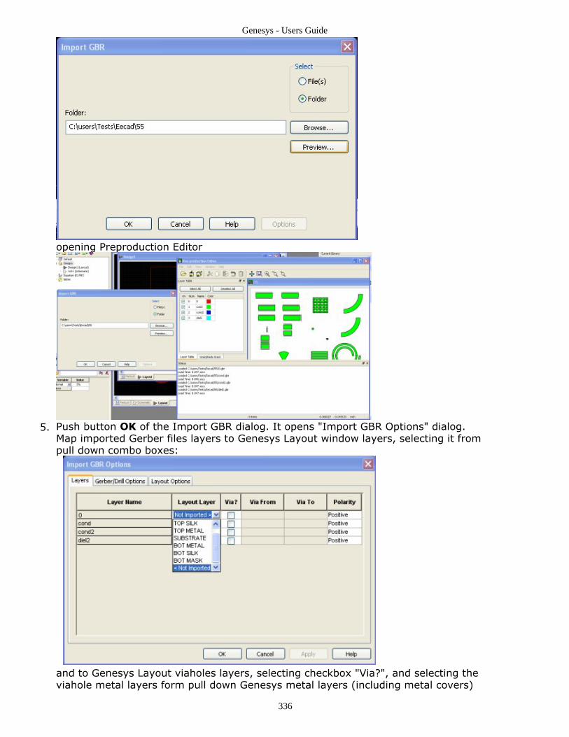
Genesys - Users Guide
336
opening Preproduction Editor
Push button OK of the Import GBR dialog. It opens "Import GBR Options" dialog.5.Map imported Gerber files layers to Genesys Layout window layers, selecting it frompull down combo boxes:
and to Genesys Layout viaholes layers, selecting checkbox "Via?", and selecting theviahole metal layers form pull down Genesys metal layers (including metal covers)

Genesys - Users Guide
337
combo boxes:
Set Gerber import options, or use default from imported Gerber/Drill files:6.
Set layout resolution options at "Layout Options" tab for importing arcs and linear7.layout object items:

Genesys - Users Guide
338
Push OK button for importing, or Cancel to cancel the operation.8.
Load Pull Data Import
M-File Import
Imported M-Files are placed in an equation block on the workspace tree.
Browse to the M-file of interest1.Click OK2.
Directory of M-Files Import
All of the M-Files located in a selected directory are imported and placed in an equationblocks on the workspace tree.
Browse to the M-file directory of interest1.Click OK2.
S-Parameter Files Import
When S-Parameters are imported a dataset is create and placed in the workspace tree.This dataset is saved and loaded with the workspace and will be cached in memory toincrease the simulation speed. The dataset can be deleted from the workspace. Memorycache will be used until there is a need to re-read the dataset from the workspace tree orif the dataset is not found the original file will be re-imported and cached once again.
S-Parameter can be imported in one of several ways detailed below:
Importing from a library
Open up the Parts Selector (Ctrl_Shift_A) or click the part selector button ( )1.Change the Current Library to the S-Parameter library of interest2.Click the library part of interest (the mouse cursor will change to a + sign)3.Place the part in the schematic by clicking the schematic4.

Genesys - Users Guide
339
NOTE: On first use of the selected library it will be unzipped and the S-Parameter file associatedwith the part will be imported into the workspace tree
Or
Importing from the Main Menu
Select File, Import, then S-Data File from the main Genesys menu1.Browse to the S-Parameter file2.Or
Importing from a Part
Place a S-Parameter part in the schematic (1-port (part), 2-port (part), n-port1.(part)). This can be done from the Linear Toolbar or the Part SelectorDouble click the part to bring up the part properties2.Click the Browse button to browse to the S-Parameter file3.
Manually Imported S-Parameters
Manually imported S-Parameters don't use a filename name. The data must exist on theworkspace tree. If the dataset is deleted then there is insufficient information to correctlybuild the model. The model has no need of the filename and simply needs to know thename of the dataset.
Place a dataset part in the schematic (NPOD (part)). This can be done from the1.Linear Toolbar or the Part SelectorDouble click the part to bring up the part properties2.Set the dataset name to the name of the imported S-Parameters3.Add an analysis and point it to the desired schematic4.Run the analysis5.
Reference
NPOD
SPICE File Import
One of the easiest ways to get nonlinear device models into Genesys is to import themfrom a manufacturer supplied SPICE file. SPICE files have the following advantages overother methods of using nonlinear device data:
They are often supplied by manufacturers.Entering device data manually is tedious and error-prone.SPICE files often contain very complete macro-model device characterizations.They are in plain text format and can be corrected in any text editor.
To import a SPICE file:
Click File on the Genesys menu and select SPICE File from the Import menu.1.Select the SPICE file and click Open.The models are imported into your workspace, but if you also want to add them to a2.design library, check Automatically import these models into library and select alibrary from the drop-down list.If you want to store the original SPICE code with the models (recommended), check3.Embed the original spice file into a notes section.

Genesys - Users Guide
340
Some devices, such as transistors, normally have their nodes reversed in the SPICE4.file. Genesys does not have enough information to know what device is described byany particular SPICE subcircuit, so you have to tell it whether the first two nodes ofany model with 3 to 5 total nodes should be reversed. Netlist options for deviceswith 3 to 5 nodes allow you to set node reversal for the whole file or receive aseparate prompt for each device found.Click OK.5.
Notes:
The import operation may take up to several minutes, depending on the number of1.models in your SPICE file. A whole library of models can reside in one file.Genesys will not allow two models with the same name in one workspace. If a name2.conflict happens, you can either replace the existing model, or rename the newmodel in the SPICE file and try importing it again.For a model with more than 5 nodes Genesyss will issue a warning (an integrated3.circuit can have a number of transposed nodes).You can edit the design's netlist in Genesys (after the model is imported) to fix the4.issues beyond the node 1 & 2 reversal.Occasionally SPICE files have errors in them, mostly simple typos. Those need to be5.corrected in a text editor prior to importing the file.
Once imported, the model can be used just like any design created in Genesys.
Quite often SPICE models are organized into a hierarchy, in which case you need to haveall of the model's dependents available in order to use the model. Sometimes dependentswill be in a different SPICE file which you will need to import into the same workspace ordesign library.
SPICE File Compatibility
SPICE file import in Genesys is mainly based on the PSpice Version 10.0 specification.Where possible, Genesys has also been made compatible with other SPICE flavors. Thefollowing devices are recognized:
C - Ideal CapacitorD - Nonlinear DiodeE - Voltage-Controlled Voltage SourceF - Current-Controlled Current SourceG - Voltage-Controlled Voltage SourceH - Current-Controlled Current SourceI - Independent Current SourceJ - Nonlinear JFETK - Mutual Inductance (coupling of two inductors only)L - Ideal InductorM - Nonlinear MOSFETQ - Nonlinear BJTR - Ideal ResistorT - Ideal Transmission LineV - Independent Voltage SourceX - SubcircuitZ - Nonlinear MESFET (model types NMF and PMF)
The intent of the SPICE file import facility in Genesys is to capture parameters of realmanufacturer parts rather than to represent more abstract models, and thus only SPICE

Genesys - Users Guide
341
commands directly related to concrete device modeling are supported: .SUBCKT, .ENDS,.MODEL and .PARAM.
Expressions are supported only as far as they are compatible with the Genesys equationparser, and .FUNC command is not supported. Also unsupported in this release are optionsVALUE, TABLE, LAPLACE, FREQ and CHEBYSHEV.
Subcircuits can have parameters, but not optional nodes, and option AKO is not supportedin models.
Based on the extensive review of available SPICE files these limitations don't seem toorestrictive, however, SPICE file compatibility will be improving in future releases.
New Spice model import supports the LEVEL keyword for JFET, MOSFET and MESFETmodels.
The value of the parameter LEVEL may be numerical or string. The string format is:
<Model Name>@<Full Path to model>
Use the string format to define an external link to a Genesys VerilogA model. Theparameter list may be unknown to Genesys, but for the import it is compiled from theVerilogA file.
For example:
ANGELOV_NFET@c:\Program Files{product-name}\Model\VerilogA\angelov.va
Note Spice import converts all SPICE file lines to upper case, while Genesys model names are casesensitive. To support the VerilogA model SPICE import, the module name in the VerilogA file must be theupper case string, otherwise after the import is performed, the model will not be found.
The numerical values of the LEVEL parameter are defined from the tables:
Table 1: MESFET models LEVEL parameter value ( TYPE = NFET, PFET)
LEVEL Model Description
0, 4 MES_<TYPE> Spice MESFET
1 CURTICE2_<TYPE> Curtice-2(quadratic)
2 STATZ_<TYPE> Statz
3 TOM_<TYPE> TOM-1
5 TOM2_<TYPE> TOM-2
6 CURTICE3_<TYPE> Curtice-3 (cubic) Table 2: MOSFET models LEVEL parameter value ( TYPE = NMOS, PMOS)

Genesys - Users Guide
342
LEVEL Model Description
0, 1 MOS1_<TYPE> Spice MOS1
2 MOS2_<TYPE> Spice MOS2
3 MOS3_<TYPE> Spice MOS3
4 BSIM1_<TYPE> Spice BSIM-1
5 BSIM2_<TYPE> Spice BSIM-2
7, 8 BSIM3_<TYPE> Spice BSIM-3
14 BSIM4_<TYPE> Spice BSIM-4 Table 3: JFET models LEVEL parameter value ( TYPE = NJF, PJF)
LEVEL Model Description
1 JFET_<TYPE> Spice JFET
2 JFET2_<TYPE> Spice JFET-2 (Parker-Skellern)
XML File Import
Each Genesys object in the workspace tree has an XML format associated with it.Workspace tree objects that have been exported to an XML format can be re-importedinto any workspace. To import an XML file:
Select the Import menu option from one of the given methods1.Click XML file2.Browse to the XML file of interest3.
6.x Model Library
Old Genesys S-Parameters
CITI file Import
Overview
CITIfile is a standardized data format that is used for exchanging data between differentcomputers and instruments. CITIfile stands for Common Instrumentation Transfer andInterchange file format.
This standard is a group effort between instrument and computer-aided design programdesigners. As much as possible, CITIfile meets current needs for data transfer, and it isdesigned to be expandable so it can meet future needs.
CITIfile defines how the data inside an ASCII package is formatted. Since it is not tied toany particular disk or transfer format, it can be used with any operating system, such asDOS or UNIX, with any disk format, such as DOS or HFS, or with any transfer mechanism,such as by disk, LAN, or GPIB.
By careful implementation of the standard, instruments and software packages usingCITIfile are able to load and work with data created on another instrument or computer. Itis possible, for example, for a network analyzer to directly load and display data measuredon a scalar analyzer, or for a software package running on a computer to read datameasured on the network analyzer.
Data Formats

Genesys - Users Guide
343
There are two main types of data formats: binary and ASCII. CITIfile uses the ASCII textformat. Although this format requires more space than binary format, ASCII data is atransportable, standard type of format which is supported by all operating systems. Inaddition, the ASCII format is accepted by most text editors. This allows files to be created,examined, and edited easily, making CITIfile easier to test and debug.
File and Operating System Formats
CITIfile is a data storage convention designed to be independent of the operating system,and therefore may be implemented by any file system. However, transfer between filesystems may sometimes be necessary. You can use any software that has the ability totransfer ASCII files between systems to transfer CITIfile data.
The descriptions and examples shown here demonstrate how CITIfile may be used tostore and transfer both measurement information and data. The use of a single, commonformat allows data to be easily moved between instruments and computers.
CITIfile Definitions
This section defines: package , header , data array , and keyword .
Package
A typical CITIfile package is divided into two parts:
The header is made up of keywords and setup information.The data usually consists of one or more arrays of data.
The following example shows the basic structure of a CITIfile package:
When stored in a file there may be more than one CITIfile package. With the Agilent 8510network analyzer, for example, storing a memory all will save all eight of the memoriesheld in the instrument. This results in a single file that contains eight CITIfile packages .
Header
The header section contains information about the data that will follow. It may alsoinclude information about the setup of the instrument that measured the data. TheCITIfile header shown in the first example has the minimum of information necessary; noinstrument setup information was included.
Data Array
An array is numeric data that is arranged with one data part per line. A CITIfile packagemay contain more than one array of data. Arrays of data start after the BEGIN keyword,and the END keyword follows the last data part in an array.

Genesys - Users Guide
344
A CITIfile package does not necessarily need to include data arrays. For instance, CITIfilecould be used to store the current state of an instrument. In that case the keywords VAR ,BEGIN , and END would not be required.
When accessing arrays via the DAC (DataAccessComponent), the simulator requires arrayparts to be listed completely and in order.
Example: S[1,1], S[1,2], S[2,1], S[2,2]
Keywords
Keywords are always the first word on a new line. They are always one continuous wordwithout embedded spaces. A listing of all the keywords used in version A.01.00 of CITIfileis shown in CITIfile Keyword Reference.
To import CITI File in Genesys:
Open File > Import > CITI File..1.
Select CITI File for Import in the Open file dialog:2.

Genesys - Users Guide
345
If the CITI file has arrays (variable, which names have indexes in square braces[]), it3.opens the dialog, defining output format of the array data.
Select Yes to convert array data in arrays, or No- otherwise:The imported file creates dataset with name = the file name in the Genesys4.workspace tree.We imported "proj.cti" CITI file, which created same named dataset:
If the workspace tree has dataset with name of the imported CITI file, then this5.dialog is opened to rename the output dataset:
For example, if CITI file has array data Si,j

Genesys - Users Guide
346
Saving its array data as Arrays will creates swept relative to independent variable freq vector PORTZ and matrix S:
otherwise the array data will be saved as scalar varaiables PORTZ_i and S_i_j:

Genesys - Users Guide
347
CITIfile Examples
The following are examples of CITIfile packages.
Display Memory File
This example shows an Agilent 8510 display memory file. The file contains no frequencyinformation. Some instruments do not keep frequency information for display memorydata, so this information is not included in the CITIfile package.
Note that instrument-specific information (#NA = network analyzer information) is alsostored in this file.
CITIFILE A.01.00
#NA VERSION HP8510B.05.00
NAME MEMORY
#NA REGISTER 1
VAR FREQ MAG 5
DATA S RI
BEGIN
-1.31189E-3,-1.47980E-3
-3.67867E-3,-0.67782E-3
-3.43990E-3,0.58746E-3
-2.70664E-4,-9.76175E-4
0.65892E-4,-9.61571E-4
END
Agilent 8510 Data File
This example shows an 8510 data file, a package created from the data register of anAgilent 8510 network analyzer. In this case, 10 points of real and imaginary data wasstored, and frequency information was recorded in a segment list table.
CITIFILE A.01.00
#NA VERSION 8510B.05.00
NAME DATA

Genesys - Users Guide
348
#NA REGISTER 1
VAR FREQ MAG 10
DATA S[1,1] RI
SEG_LIST_BEGIN
SEG 1000000000 4000000000 10
SEG_LIST_END
BEGIN
0.86303E-1,-8.98651E-1
8.97491E-1,3.06915E-1
-4.96887E-1,7.87323E-1
-5.65338E-1,-7.05291E-1
8.94287E-1,-4.25537E-1
1.77551E-1,8.96606E-1
-9.35028E-1,-1.10504E-1
3.69079E-1,-9.13787E-1
7.80120E-1,5.37841E-1
-7.78350E-1,5.72082E-1
END
Agilent 8510 3-Term Frequency List Cal Set File
This example shows an 8510 3-term frequency list cal set file. It shows how CITIfile maybe used to store instrument setup information. In the case of an 8510 cal set, a limitedinstrument state is needed to return the instrument to the same state that it was in whenthe calibration was done.
Three arrays of error correction data are defined by using three DATA statements. Someinstruments require these arrays be in the proper order, from E[1] to E[3] . In general,CITIfile implementations should strive to handle data arrays that are arranged in anyorder.
CITIFILE A.01.00
#NA VERSION 8510B.05.00
NAME CAL_SET
#NA REGISTER 1
VAR FREQ MAG 4
DATA E[1] RI
DATA E[2] RI
DATA E[3] RI
#NA SWEEP_TIME 9.999987E-2
#NA POWER1 1.0E1
#NA POWER2 1.0E1
#NA PARAMS 2
#NA CAL_TYPE 3
#NA POWER_SLOPE 0.0E0
#NA SLOPE_MODE 0
#NA TRIM_SWEEP 0
#NA SWEEP_MODE 4
#NA LOWPASS_FLAG -1
#NA FREQ_INFO 1
#NA SPAN 1000000000 3000000000 4
#NA DUPLICATES 0
#NA ARB_SEG 1000000000 1000000000 1
#NA ARB_SEG 2000000000 3000000000 3
VAR_LIST_BEGIN
1000000000
2000000000
2500000000
3000000000
VAR_LIST_END
BEGIN
1.12134E-3,1.73103E-3
4.23145E-3,-5.36775E-3

Genesys - Users Guide
349
-0.56815E-3,5.32650E-3
-1.85942E-3,-4.07981E-3
END
BEGIN
2.03895E-2,-0.82674E-2
-4.21371E-2,-0.24871E-2
0.21038E-2,-3.06778E-2
1.20315E-2,5.99861E-2
END
BEGIN
4.45404E-1,4.31518E-1
8.34777E-1,-1.33056E-1
-7.09137E-1,5.58410E-1
4.84252E-1,-8.07098E-1
END
When an instrument's frequency list mode is used, as it was in this example, a list offrequencies is stored in the file after the VAR_LIST_BEGIN statement. The unsortedfrequency list segments used by this instrument to create the VAR_LIST_BEGIN data aredefined in the #NA ARB_SEG statements.
2-Port S-Parameter Data File
This example shows how a CITIfile can store 2-port S-parameter data. The independentvariable name FREQ has two values located in the VAR_LIST_BEGIN section. The fourDATA name definitions indicate there are four data arrays in the CITIfile package locatedin the BEGIN...END sections. The data must be in the correct order to ensure values areassigned to the intended ports. The order in this example results in data assigned to theports as shown in the table that follows:
CITIFILE A.01.00
NAME BAF1
VAR FREQ MAG 2
DATA S[1,1] MAGANGLE
DATA S[1,2] MAGANGLE
DATA S[2,1] MAGANGLE
DATA S[2,2] MAGANGLE
VAR_LIST_BEGIN
1E9
2E9
VAR_LIST_END
BEGIN
0.1, 2
0.2, 3
END
BEGIN
0.3, 4
0.4, 5
END
BEGIN
0.5, 6
0.6, 7
END
BEGIN
0.7, 8
0.8, 9
END

Genesys - Users Guide
350
DATA FREQ = 1E9 FREQ = 2E9
s[1,1] s[0.1,2] s[0.2,3]
s[1,2] s[0.3,4] s[0.4,5]
s[2,1] s[0.5,6] s[0.6,7]
s[2,2] s[0.7,8] s[0.8,9]
CITIfile Keyword Reference
The following table lists keywords, definitions, and examples.
h7. CITIfile Keywords and Definitions

Genesys - Users Guide
351
Keyword Example and Explanation
CITIFILE Example: CITIFILE A.01.00Identifies the file as a CITIfile and indicates the revision level of the file. The CITIFILEkeyword and revision code must precede any other keywords.The CITIFILE keyword at the beginning of the package assures the device reading the filethat the data that follows is in the CITIfile format.The revision number allows for futureextensions of the CITIfile standard.The revision code shown here following the CITIFILE keyword indicates that the machinewriting this file is using the A.01.00 version of CITIfile as defined here. Any future extensionsof CITIfile will increment the revision code.
NAME Example: NAME CAL_SETSets the current CITIfile package name. The package name should be a single word with noembedded spaces. Some standard package names:RAW_DATA : Uncorrected data.DATA: Data that has been error corrected. When only a single data array exists, it should benamed DATA .CAL_SET: Coefficients used for error correction.CAL_KIT: Description of the standards used.DELAY_TABLE: Delay coefficients for calibration.
VAR Example: VAR FREQ MAG 201Defines the name of the independent variable ( FREQ ); the format of values in aVAR_LIST_BEGIN table ( MAG ) if used; and the number of data points ( 201 ).
CONSTANT Example: CONSTANT name valueLets you record values that do not change when the independent variable changes.
# Example: #NA POWER1 1.0E1Lets you define variables specific to a particular type of device. The pound sign ( # ) tells thedevice reading the file that the following variable is for a particular device.The device identifier shown here ( NA ) indicates that the information is for a networkanalyzer. This convention lets you define new devices without fear of conflict with keywordsfor previously defined devices. The device identifier can be any number of characters.
SEG_LIST_BEGIN Indicates that a list of segments for the independent variable follows.Segment Format: segment type start stop number of pointsThe current implementation supports only a signal segment. If you use more than onesegment, use the VAR_LIST_BEGIN construct. CITIfile revision A.01.00 supports only the SEG(linear segment) segment type.
SEG_LIST_END Sets the end of a list of independent variable segments.
VAR_LIST_BEGIN Indicates that a list of the values for the independent variable (declared in the VARstatement) follows. Only the MAG format is supported in revision A.01.00.
VAR_LIST_END Sets the end of a list of values for the independent variable.
DATA Example: DATA S[1,1] RIDefines the name of an array of data that will be read later in the current CITIfile package ,and the format that the data will be in. Multiple arrays of data are supported by usingstandard array indexing as shown above. CITIfile revision A.01.00 supports only the RI (realand imaginary) format, and a maximum of two array indexes.Commonly used array names include:S - S parameterE - Error TermVoltage - VoltageVOLTAGE_RATIO - a ratio of two voltages (A/R)
CITIfile Guidelines
The following general guidelines aid in making CITIfiles universally transportable:
Line Length. The length of a line within a CITIfile package should not exceed 80characters. This allows instruments which may have limited RAM to define a reasonableinput buffer length.

Genesys - Users Guide
352
Keywords. Keywords are always at the beginning of a new line. The end of a line is asdefined by the file system or transfer mechanism being used.
Unrecognized Keywords. When reading a CITIfile, unrecognized keywords should beignored. There are two reasons for this:
Ignoring unknown keywords allows new keywords to be added, without affecting anolder program or instrument that might not use the new keywords. The olderinstrument or program can still use the rest of the data in the CITIfile as it didbefore. Ignoring unknown keywords allows "backwards compatibility" to bemaintained.Keywords intended for other instruments or devices can be added to the same filewithout affecting the reading of the data.
Adding New Devices. Individual users are allowed to create their own device keywordsthrough the # (user-defined device) mechanism. (Refer to the table immediately abovefor more information.) Individual users should not add keywords to CITIfiles without usingthe # notation, as this could make their files incompatible with current or future CITIfileimplementations.
File Names. Some instruments or programs identify a particular type of file by charactersthat are added before or after the file name. Creating a file with a particular prefix orending is not a problem. However in general an instrument or program should not requireany such characters when reading a file. This allows any file, no matter what the filename,to be read into the instrument or computer. Requiring special filename prefixes andendings makes the exchange of data between different instruments and computers muchmore difficult.
A CITIfile package is as described in the main CITIfile documentation: the CITIFILEkeyword, followed by a header section, usually followed by one or more arrays of data.
NoteThere are some specific problems with the current version in reading and/or writing this data format. Onthe Agilent EEsof web site, refer to the Release Notes in Product Documentation, and to Technical Supportfor more information and workarounds (http://www.agilent.com/find/eesof ).
Generic MDIF Format
The generic MDIF provides a generalized MDIF format for unifying the various specificMDIF formats, and overcoming some limitations of other formats. The generic formatenables diverse applications to use a common data I/O interface, so long as the intent isto access/save multidimensional (multiple independent vs dependent variables) data.
The general format is as follows:
VAR var1Name(var1Type) = var1
ValueVAR var2Name(var2Type) = var2Value
..
VAR varNName(varNType) = varNValue
BEGIN blockName
% bVar1Name(bVar1Type) bVar2Name(bVar2Type) ....
% bVarLName(bVarLType) ...
% ...
% bVarQName(bVarQType) ... bVarPName(bVarPType)

Genesys - Users Guide
353
bVar1Value bVar2Value ...
bVarLValue ..
..
bVarQValue ... bVarPValue
bVar1Value bVar2Value ...
bVarLValue ..
..
bVarQValue ... bVarPValue
...
END
where var*Type can be the token:
0 or int1 or real2 or string
Type bVar*Type can be one of the above as well as:
3 or complex4 or boolean5 or binary6 or octal7 or hexadecimal8 or byte16
The variable names above constitute a name-space uniquely identified by the stringblockName which is either:
alphanumeric: all bVar*Name block variables are dependent, except bVar1Name,which is usually the most rapidly changing (innermost) independent variable.orDSCR(blockName): all bVar*Name block variables are dependent, and there is anindexing implicit independent variable.
Guidelines
A string type variable's value must be surrounded by "".
If there are multiple blocks, the outermost independent variables (e.g., VARvar1Name(var1Type) = var1 ) apply only to the block immediately following thevariable definitions, and not to any other blocks.
The block data (bVar*Value) lines must follow the pattern (order, number of valuesper line, and number of lines) of the format (%) lines. If the number of values in anydata line does not match the number of dependent variables specified in thecorresponding format (%) line, incorrect results will occur. A variable's value cannotbe split across lines. Although there is no line length limit specified, MDIF file readersmay choose to truncate at some finite length. This may result in a file read error, or,if the file was carefully crafted, truncated names and/or string-type values.
Scale factors, which can be applied only to real numbers, may be case-insensitivesuffixes as follows:
f = 1e-15, p = 1e-12, n = 1e-9, u = 1e-6, mil = 2.54e-5, m = 1e-3,
k = 1e3, g = 1e9, t = 1e12

Genesys - Users Guide
354
E.g.: 15mA = 15e-3, 30KHz = 30e3
There should be no space between the number and the suffix, and extra charactersare ignored. Unrecognized suffixes result in 1.0. The above is not totally consistentwith the rest of ADS.
The format of complex data is real/imag, with a column for real and a column forimaginary.
Multidimensional data is organized by outer to inner independent variables. VARstatements go from outermost to innermost.
Vary innermost independent variables first, proceeding toward outermost variableschanging last.
Independent variables should change monotonically.
Example
!============================================================
! Example 1
REM This has 3 indepVars: v1, v2, v3(innermost) and
REM 4 depVars: dv1(integer), dv2(real), dv3(string) and
REM dv4(hexadecimal), but is read in as a string.
REM The outermost indepVars: v1, v2 apply only to the block
REM immediately following them, and not to any other block.
! There are 2 data nodes
VAR v1(0) = 1
VAR v2(1) = 2.2
BEGIN blk1
% v3(1) dv1(1) dv2(1) dv3(2) dv4(hexadecimal)
7.7 8 9.9999 "line 1" 0xabc
8.8 9 1.11 "line 2 " 0x123
END
VAR v1(0) = 2
VAR v2(1) = 3.2
BEGIN blk1
% v3(1) dv1(1) dv2(1) dv3(2) dv4(hexadecimal)
8.7 9uF 10.9999mA "line 1" 0xff
9.8 10uF 11.11mA "line 2 " 0xdef
END
!=============================================================
! Example 2
! Created Tue Mar 9 13:39:19 1999
! Data Acquired Tue Mar 9 13:38:34 1999
BEGIN NDATA_noise
% freq(real) Sopt(complex) NFmin(real) Rn(real) PortZ[1](real)
1e+09 0.098481 0.017365 1 5 50
2e+09 0.18794 0.068404 2 10 50
3e+09 0.25981 0.15 3 15 50
4e+09 0.30642 0.25712 4 20 50
5e+09 0.32139 0.38302 5 25 50
6e+09 0.3 0.51962 6 30 50
7e+09 0.23941 0.65778 7 35 50
8e+09 0.13892 0.78785 8 40 50
9.543e+09 -0.014122 0.911 9.5445 46.166 50
END

Genesys - Users Guide
355
X-parameter GMDIF Format
This section describes:
Choosing an X-parameter file for use with an X-Parameter partAn overview of the X-parameter fileExamples of various details in X-parameter files
Overview
These files contain X-parameter data for nonlinear n-port devices, or subcircuits. They areASCII files in GMDIF format. They use extension: .xnp.The X-parameter files completely comply by Generic MDIF Format. The specific block andvariable names used in the X-parameter GMDIF files are described in this section.This section describes Version 2.0 X-parameter GMDIF files.An X-parameter GMDIF file can be used with an X-Parameter part to model the behaviorof a nonlinear device or subcircuit using X-parameters. The file contains the X-parameters,the part is placed within the schematic.
Linking an X-parameters GMDIF File to an X-parameters Part
To link a file to the part:
Add X-parameters part to your schematic. It can be found in the RF Design library.1.Set up the X-parameters parameters. For instructions on how to set the parameters,2.click Model Help in the part's dialog box.
Comments
GMDIF files support comments in two ways:
by using "!" orby using "REM" statement.
The "!" can be used in the beginning of a line, or at the end of the line where as, "REM"can be used only in the beginning of a line.Version 2.0 X-parameter GMDIF files contain a pre-defined comment section at thebeginning of the files, which provides useful information about the range of operatingconditions covered by the data as shown in the example below:
Example
! Created Fri Jul 10 15:29:17 2009
! Version = 2.0
! HB_MaxOrder = 9
! XParamMaxOrder = 3
! NumExtractedPorts = 3
! fund_1=[1e+09->1.4e+09] NumPts=5
! VDC_3=[10->11] NumPts=2
! ZM_2_1=50 NumPts=1
! ZP_2_1=0 NumPts=1
! AN_1_1=[3.16228e-03(-20.000000dBm)->70.7107e-03(6.989700dBm)] NumPts=36
The version of the file is stated just for convenience. The statement determining theversion is elsewhere. The comment "HB_MaxOrder = 9" tells you that the Harmonic

Genesys - Users Guide
356
Balance with MaxOrder=9 was used by X-Parameter Generator. The comment"XParamMaxOrder = 3" tells you that the X-parameter data in this file contains mixingindices up to the 3rd order.The comment "NumExtractedPorts = 3" indicates the total number of ports used for X-parameter generation. In case of non-consecutive port numbering this value may besmaller than the highest port number.The lower part of this comment section indicates various independent variables togetherwith the covered sweeps for each of them. See X-parameter Independent Variables(users) for explanation of the variable names.
X-parameter GMDIF File Blocks
Version 2.0 of X-parameter GMDIF files contains three types of blocks:
XParamAttributesXParamPortDataXParamData
The first two blocks appear only once in the file. The third block appears as many times asthe number of distinct different sweep points present in the data for all but the innermostindependent variable. The following sections provide details for these blocks.
XParamAttributes Block
The XParamAttributes block provides the vehicle for the official statements of (1) thefile version, (2) the number of ports, and (3) the number of fundamental frequencies(tones).
Example
BEGIN XParamAttributes
% Index(int) Version(real) NumPorts(int) NumFundFreqs(int)
0 2.0 3 1
END
The sole purpose of the Index column is compliance with the Generic MDIF format.The NumPorts entry indicates the highest port index in the data.
XParamPortData Block
The XParamPortData block provides reference impedances for the incident and reflectedwaves at each port covered by the data. The reference impedances can be complex andthe power definition of the waves is used, as follows:
In the above equations, Vp and Ip represent amplitude phasors.
Example
BEGIN XParamPortData
% PortNumber(int) RefZ0(complex) PortName(string)
1 50 0 "Input"
2 50 0 "Output"

Genesys - Users Guide
357
3 50 0 "VDC"
END
The XParamPortData block also includes the port names. This information is particularlyuseful in proper hookup of the X-parameters part in cases where more than two portsare present and a mixture of port types is used.
XParamData Block
The XParamData block provides the actual X-parameters. This block may appear manytimes in the file, each containing X-parameters at one sweep point (of all but theinnermost independent variable) at a time.Each XParamData block is preceded by m-1 VAR statements for m-1 independentvariables, where m is the total number of independent variables. These VAR statementsprovide the types and the values of the independent variables. These values apply to theXParamData block immediately following the VAR statements, and only to that block.
Example
VAR fund_1(real) = 1e+09
VAR VDC_3(real) = 10
VAR ZM_2_1(real) = 50
VAR ZP_2_1(real) = 0
BEGIN XParamData
% AN_1_1(real) FI_3(real) FB_1_1(complex) ...
...
...
...
END
The last, mth, independent variable is the innermost variable and is placed as the firstvariable inside the block. In the above example that variable is "AN_1_1".The naming convention for the independent variables in X-parameter files is described inX-parameter Independent Variables (users).All the dependent variables (the X-parameters) are provided inside the block. Followingthe mth independent variable, the names and the types of the dependent variables arespecified in the header lines (lines starting with a "%" character). The header lines arespecified once per block at the beginning of the block. They are then followed by as manydata groups as the number of sweep points of the innermost independent variable. Eachgroup consists of data values formatted into lines exactly in the same way as the blockheader lines with each entry representing a value of the correspondingly placed variable inthe header lines. Complex data is specified in the rectangular format (real, imaginary) bytwo numbers.
Example
VAR fund_1(real) = 1e+09
VAR VDC_3(real) = 10
VAR ZM_2_1(real) = 50
VAR ZP_2_1(real) = 0
BEGIN XParamData
% AN_1_1(real) FI_3(real) FB_2_1(complex) S_1_2_2_2(complex)
0.0657 -0.32 0.113 1.01 0.222 -0.0031
0.0667 -0.33 0.111 1.02 0.222 -0.0034
0.0677 -0.34 0.110 1.05 0.222 -0.0039
END
In the above example the complex number (0.111 + j1.02) is the value of the dependent

Genesys - Users Guide
358
variable FB_2_1 at the multidimensional point established by all the values of theindependent variables, including the value of 0.0667 of AN_1_1.The naming convention for the dependent variables in X-parameter files is described in X-parameter Dependent Variables (users).
X-parameter Variables
Notation
All independent and dependent variables are defined with respect to port and harmonic (ormixing) indices. For each variable these indices, separated by the underscore character "",form a string appending the reserved name of the variable. Negative indices, if allowed,are represented by a string in which the "m" character is used in place of the minus ("-")sign, with no space between the sign and the number. For example "_m2" represents theindex "-2". For clarity of presentation the following table shows the notation used inindexing the X-parameters.
k fundamental frequency index; 1 in the case of single tone X-parameters;all consecutive numbers must bepresent
p port index - a positive integer; may not be consecutivepIn - denotes the "input" port indexpOut - denotes the "output" port index
n harmonic index; positive integernIn - denotes the harmonic on the "input" portnOut - denotes the harmonic on the "output" portin case of multi-tone X-parameters there is a mixing index that is concatenated from harmonic indicesw.r.t. to subsequent fundamentals, for example "_1_m2_2" in the three-tone case refers to the mixingproduct f1-2f2+2f3 - the index w.r.t. the first fundamental is expected to be non-negative and all-zeroentries are not allowed.
Independent Variables
The following table lists all the supported independent variables in Version 2.0 X-parameter files. In general, all X-parameters are functions of some or all of theseindependent variables. Their dependence is tabulated in the X-parameter files for allsweep points of the independent variable values.All independent variables are real numbers.

Genesys - Users Guide
359
fund_k kth fundamental frequency; assumed non-commensurate if more than one is present; fund_1 isrequired
VDC_p DC voltage applied to port p; not required; mutually exclusive with IDC_p at the same port p
IDC_p DC current applied to port p; not required; mutually exclusive with VDC_p at the same port p
AN_p_n magnitude of a large-signal incident wave applied to port p at harmonic n; only one per eachfundamental is both allowed and required; phase of this incident wave is not tabulated in the X-parameter files as this incident wave serves as a Reference Signal (Refer to ADS document fordetailed description); power definition of incident waves is used
AM_p_n magnitude of any other than Reference Signal large-signal incident wave applied to port p atharmonic n; required only if AP_p_n is used at the same port p and harmonic n; power definition ofincident waves is used
AP_p_n phase in degrees of any other than Reference Signal large-signal incident wave applied to port p atharmonic n; required only if AM_p_n is used at the same port p and harmonic n
GM_p_n magnitude of the reflection coefficient of the load at port p and harmonic n; required only if GP_p_nis used at the same port p and harmonic n; power definition of the reflection coefficient and thereference impedance specified for port p are used; mutually exclusive with other formats ofspecifying load at the same port p and harmonic n
GP_p_n phase in degrees of the reflection coefficient of the load at port p and harmonic n; required only ifGM_p_n is used at the same port p and harmonic n; mutually exclusive with other formats ofspecifying load at the same port p and harmonic n
GX_p_nGY_p_n
alternative to GM_p_n and GP_p_n; real and imaginary parts of the reflection coefficient; mutuallyexclusive with other formats of specifying load at the same port p and harmonic n
ZM_p_nZP_p_n
alternative to GM_p_n and GP_p_n; magnitude and phase of the load impedance; mutually exclusivewith other formats of specifying load at the same port p and harmonic n
ZX_p_nZY_p_n
alternative to GM_p_n and GP_p_n; real and imaginary parts of the load impedance; mutuallyexclusive with other formats of specifying load at the same port p and harmonic n
Dependent Variables
The following table provides the notation for the dependent variables (X-parameters) usedin Version 2.0 X-parameter files. The X-parameters can be either real or complexnumbers. In the latter case the rectangular format (real and imaginary parts) is used. It isnot essential for any specific dependent variable to be present in an X-parameter file. Ingeneral, the default value is zero for any absent parameter that could otherwise beincluded in the file (some parameters are mutually exclusive with some otherparameters).

Genesys - Users Guide
360
FB_pOut_nOut complex B-type X-parameter - measured reflected wave at output port pOut andharmonic nOut as the response to all large-signal excitations (i.e., under thelarge-signal operating conditions); power definition of the reflected waves isused
FI_pOut real I-type X-parameter - DC current measured at output port pOut under thelarge-signal operating conditions
FV_pOut real V-type X-parameter - DC voltage measured at output port pOut under thelarge-signal operating conditions
S_pOut_nOut_pIn_nIn complex S-type X-parameter providing the small-signal added-contribution to thereflected wave at output port pOut and harmonic nOut due to a small-signalincident wave at input port pIn and harmonic nIn measured under the large-signal operating conditions; power definition of the incident and reflectedwaves is used
T_pOut_nOut_pIn_nIn complex T-type X-parameter providing the small-signal added-contribution to thereflected wave at output port pOut and harmonic nOut due to a phase-reversed small-signal incident wave at input port pIn and harmonic nInmeasured under the large-signal operating conditions; power definition ofthe incident and reflected waves is used
XY_pOut_pIn_nIn complex Y-type X-parameter providing the small-signal contribution to the DC currentat output port pOut due to a small-signal incident wave at input port pIn andharmonic nIn measured under the large-signal operating conditions; powerdefinition of the incident waves is used; the real-valued contribution to theDC current is the real part of complex product of this X-parameter and thecorresponding incident wave
Yre_pOut_pIn_nInYim_pOut_pIn_nIn
realreal
alternative to XY_p_n, obsolete in Version 2.0 X-parameter files; two realnumbers: the real part and negative of the imaginary part are providedinstead of one complex number, as XY = Yre - j*Yim
XZ_pOut_pIn_nIn complex Z-type X-parameter providing the small-signal contribution to the DC voltageat output port pOut due to a small-signal incident wave at input port pIn andharmonic nIn measured under the large-signal operating conditions; powerdefinition of the incident waves is used; the real-valued contribution to theDC voltage is the real part of complex product of this X-parameter and thecorresponding incident wave
Zre_pOut_pIn_nInZim_pOut_pIn_nIn
realreal
alternative to XZ_p_n, obsolete in Version 2.0 X-parameter files; two realnumbers: the real part and negative of the imaginary part are providedinstead of one complex number, as XZ = Zre - j*Zim
Restrictions
If the independent variable VDC_pOut is specified for the port pOut then neither the V-type (FV_pOut) nor the Z-type (XZ_pOut_pIn_nIn, Zre_pOut_pIn_nIn, Zim_pOut_pIn_nIn) X-parameters can be specified for the port pOut.Similarly, if the independent variable IDC_pOut is specified for the port pOut then neitherthe I-type (FI_pOut) nor the Y-type (XY_pOut_pIn_nIn, Yre_pOut_pIn_nIn,Yim_pOut_pIn_nIn) X-parameters can be specified for the port pOut.
Exporting Files Using GenesysGenesys can export the following file types:
ASCII Drill ListExport Schematics to ADSBill of MaterialsBitmap (Active Window)Bitmap (Entire Screen)DXF/DWG FileGDSII FileGerber FileHPGL File

Genesys - Users Guide
361
IFF Schematic FilePart Placement ListS-ParametersSPICE FileTouchstone FileXML File
Export a file
To export a file please follow the following steps detailed below:Select the object in the Workspace Tree to be exported.Click File on the Genesys menu and select a file type from the Export menu.Follow the instructions in the windows that appear.OrRight click on the object in the Workspace Tree to be exported.Select the Export menu.Follow the instructions in the windows that appear.
ASCII Drill List Export
Schematics to ADS Export
Bill of Materials Export
Bitmap (Active Window) Export
A bitmap of the active window can be exported. To export the active window:
Open the window and make sure it is the active window1.Select the File > Export > Bitmap (Active Window) menu2.When prompted specify the directory and filename3.
Bitmap (Entire Screen) Export
A bitmap of the entire screen can be exported. To export the entire screen:
Select the File > Export > Bitmap (Entire Screen) menu1.When prompted specify the directory and filename2.
DXF/DWG File Export
The Export DXF/DWG Options dialog box enables you to set file format, Autocad version,path geometry, and hole format.

Genesys - Users Guide
362
To export AutoCAD DXF/DWG files:In the layout window containing your design, choose File > Export > DXFFile...
It opens Export DXF Options dialog. Select exported layers in the Layers tab(default - all layers are selected)
Select exporting DXF Options: output File Format DXF(Text) or DWG(Binary),AutoCAD version, format of Holes, and format pf Paths.

Genesys - Users Guide
363
At the Layout Options tab define exporting Layout objects (components, EM-ports, drill holes). To convert all layout objects to resolved polygons (exceptinglayers with text), set checkbox Convert all shapes into resolved polygons.
Close the dialog by OK button opens Export DXF (or Export DWG) file openingdialog. Enter full path to output file manually, or using Browse button. Selectbox View File after export to view output file after export.

Genesys - Users Guide
364
Push OK button. After export it opens Preproduction editor, displaying results ofthe export:

Genesys - Users Guide
365
Genesys Error/Messages window displays results of the export:
GDSII File Export
Gerber File Export
HPGL File Export
IFF Schematic File Export
Export any schematic created in Genesys to another program using Interchange FileFormat (IFF). This lets you use your schematic in programs other than Genesys, such asADS.

Genesys - Users Guide
366
Exporting IFF Files That are ADS Compatible
Only schematics are supported for export to IFF files.
Note: Schematics that you manually create should import into ADS. If you have any compatibility issues,please contact Agilent directly.
To export a schematic to an IFF file:
Open a schematic.1.Click File on the Genesys menu and select*IFF Schematic File* from the Export2.menu.Save the file in .iff format.3.Now open the IFF file in ADS.4.
Translating Direct Parts to IFF
When a part in Genesys is the same as a part in ADS, Genesys uses that ADS part. Partsare considered the same if:
The part symbols are exactly the same size.The parameters are compatible. The parameter names do not have to match exactly,but the parameters from Genesys must be convertible with a simple mapping table orformulas.
For example, a resistor maps to IFF because the standard resistor size is one inch and theparameter R (resistance) has a standard meaning.
Translating Custom Parts to IFF
If a part does not directly translate to IFF, Genesys creates a custom part and symbol inADS. This creates an additional network in ADS, and possibly a netlist file, to support thenew part. These custom networks use a standard naming convention so that your ADSdesigns are easily shared and edited.
Translating DisCos to IFF
While DisCos are not directly supported in ADS, Genesys recreates these parts with theadditional terminals necessary for ADS compatibility. All DisCos work in ADS withoutmanual modifications.
Exporting Other Items to IFF
In addition to a schematic, other items are automatically exported to IFF files. Theseinclude:
All equationsSubstrates used by the schematicLinear simulations
Using Custom Mapping Files for IFF Export
Genesys IFF file export is controlled by a sophisticated internal mapping file. You cancreate a user mapping file if you want to customize the IFF export. For more information

Genesys - Users Guide
367
on this mapping file and customization services, please contact Agilent or your localdistributor.
Part Placement List Export
S-Parameters Export
Noise parameters are not exported with the S-Parameters.
S-Parameters can be exported in one of two ways.
Exporting from the Workspace Tree
Right click the linear analysis dataset in the workspace tree and select Export from1.the menuSet the name and directory of the S-Parameter file (*.snp)2.Or
Exporting from the Dataset Window
Open the linear analysis dataset (it must be the active window)1.Select File, Export, and then S-Parameters from the Genesys menu2.Set the name and directory of the S-Parameter file (*.snp)3.
SPICE File Export
SPICE files are exported from a schematic. This is because many SPICE device models aresignificantly different from linear simulator models. Terminations are often handleddifferently in SPICE and linear simulators. In Genesys, oscillators are analyzed open loopwhile the loop is closed for SPICE analysis. These differences are resolved in theschematic.
Translating Parts to SPICE
There are three categories of part translation to SPICE:
DirectCompoundIncompatible
For translations of specific parts, see the Part Catalog (part).
Direct - Direct parts are translated on a one-to-one basis. Examples include capacitors,inductors, resistors, signal ground (DC voltage source), and electrical transmission lines.
Compound - Compound parts are translated as SPICE subcircuits. They include mutualinductors , op-amps , VCC , and Crystal. This provides comparable simulations in Genesysand SPICE. For example, an Genesys VCC is modeled by two resistors and a voltagecontrolled current source. To use just the SPICE VCC device without the resistors, you canoverride the default translation by double-clicking the VCC device to open the propertieswindow. Select G from the SPICE Device list and click OK to save the changes.
Please note the following:
The SPICE opamp E model (Genesys translates OPA as an E model) is ideal in that

Genesys - Users Guide
368
the unity crossover frequency is infinite. You can substitute a SPICE library model orsubcircuit for the opamp. Most opamp manufacturers have SPICE models for theirproducts.The Genesys TRF device (ideal transformer) is not supported in SPICE. You shouldspecify mutually coupled inductors (MUI). You need to specify appropriate windinginductance and coupling.The Genesys FET and BIP devices do not include any biasing information and,therefore, are not translated. You can specify how to translate these parts by definingthe translation device in the properties window.
Incompatible - Incompatible parts are those parts that have no simple SPICE equivalent,including physical models, S-parameter or Y-parameter devices, and internal transistormodels (FET and BIP). Incompatible parts are identified in the translated SPICE file withan exclamation point (!) at the front of the part line. You can assign a SPICE model(.MODEL) or subcircuit to that part in the properties window.
You must also place a SPICE model definition (.MODEL block) in the exported SPICE file.This is done either through SPICE command text or manually after exporting. If the SPICEsimulator supports libraries (both PSPICE and IsSPICE support libraries), the libraryreference is included in SPICE command text entries.
Touchstone File Export
Touchstone circuit files are similar to Genseys netlists and are generally a one-to-onetranslation.
XML file Export
Each Genesys object in the workspace tree has an XML format associated with it.Workspace tree objects that can be exported to an XML format. To export an XML file:
Click the object in the workspace tree to be exported1.Select the Export menu option from one of the given methods2.Specify the name of the directory and filename of the exported object3.
Layout DesignsThere are several tools available to you to help with the export/conversion of LayoutDesigns.
AutoCAD DXF/DWG Translator
The DXF/DWG translator enables you to convert Genesys designs into AutoCAD'sDXF/DWG file format, as well as convert DXF/DWG files into Genesys designs. DXF is avery simple file format that can be read by most CAD programs that support DXF. TheDXF/DWG translator is bidirectional and provides support for hierarchical and all layerseparation.
DWG is a binary format, therefore the files take less time to load and save. Genesyssupports importing and exporting to/from AutoCAD. AutoCAD versions 12 to 2007 aresupported for import. AutoCad versions 2000, 2004 and 2007 are supported for export.Carefully consider how you want to use DXF/DWG output - including layer numbering, useof holes, and polygon shapes - before beginning your layout Layout. Setting up the properlayout rules in Genesys can save a lot of time in generating acceptable DXF/DWG output.For specific considerations or limitations, consult your AutoCAD documentation.

Genesys - Users Guide
369
Note: Password protected DWG files are not supported.
Genesys includes an editor that can display the DXF/DWG Layout. Using the editor, youcan compare the DXF/DWG files to the original Genesys layout Layout to verify that theLayout was exported correctly. Similarly, DXF/DWG files can be previewed prior to importinto Genesys:
to edit a large Layout down to a smaller Layout prior to importing it into Genesys.This edited Layout can be saved and then imported in Genesys.or after import, to verify that the DXF/DWG Layout data and the Gensys-importedLayout appear similar.
For details, see Using the Pre-Production Editor.
Export Layout Options
We can show up Layout options settings, defining exporting Layout objects (components,EM-ports, drill holes).
Converting to resolved polygons (Export ports = Yes):1.All layout objects are converted to polygons, which are resolved to polygon unions for2.all layers, not having text objects.
Exporting without converting to "resolved polygons" (Export ports = Yes):3.All layout objects are mapped to output "as is", without converting to polygons.
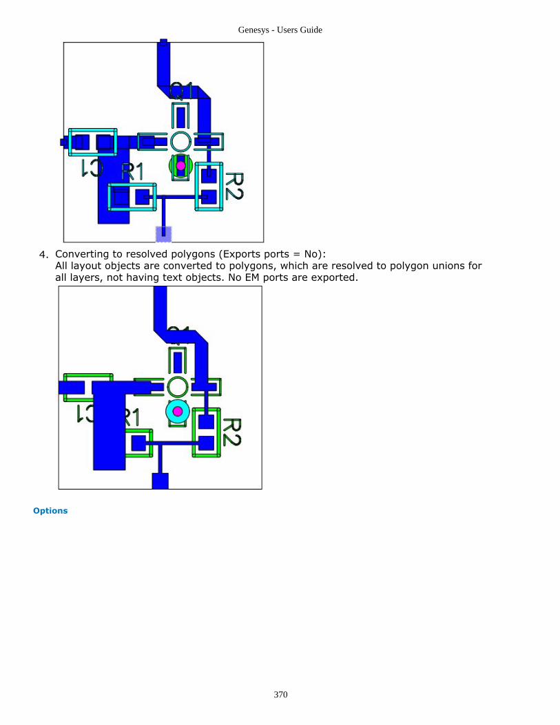
Genesys - Users Guide
370
Converting to resolved polygons (Exports ports = No):4.All layout objects are converted to polygons, which are resolved to polygon unions forall layers, not having text objects. No EM ports are exported.
Options

Genesys - Users Guide
371
File format
DXF (Text) Select this option to export the Genesys Layout to DXF format as an ASCII text file. This selectionis the default setting.
DWG Select this option to export your Genesys Layout to a binary DWG file format. Exporting to DWGfile format is faster than the DXF (Text) format. Also file size of the DWG file will be smaller ascompared to corresponding DXF (Text) file.
Autocadversion
Use this drop-down list to select the AutoCad version. Genesys layout can be exported in threeAutoCad versions: 2000, 2004, and 2007.
Paths aspolygons
Select Paths As Polygons to export the Layout paths or traces as polygons. Paths or traces havemitered or curved corners that need to be preserved in the translation. The Genesys layout haspaths with endpoint types other than flush that need to be preserved in the program database.This option is selected as the default.
Holeformat
The Hole format section enables you to define how the translator deals with holes in a Layout.
Holes aspolygons
Select Holes As polygons to convert holes into polygons. One polygon will be created for eachhole in the same layer.
NoteSome systems may not be able to tolerate complex polygons with cutlines. For these systems, selectHoles as polygons. This option is deselected as the default.
Holes ascutlines
Select Holes as cutlines to convert holes into cutlines. This option is selected as thedefault.
Gerber Translator
The Gerber Artwork Translator can translate artwork directly from circuit layouts createdwith Genesys Layout editor into Gerber format. It exports Genesys layouts into ASCII filesthat control Gerber photoplotting equipment.
Genesys includes an editor that can display the Gerber/Drill design. Using the editor, youcan compare the Gerber/Drill files to the original Genesys layout design to verify that thedesign was exported correctly.
For details, see Using the Pre-Production Editor.
Gerber Command Format
The Gerber format is a numerical control language developed to generate photo artwork.The output of this translator is an ASCII file that contains the following Gerber commands:
G01 = linear interpolationG54 = aperture selectD01 = shutter openD02 = shutter closeD03 = flashM02 = end of programX and Y = coordinates* = end of block
Coordinates are absolute, with implied decimal point and optional leading zerosuppression. However, the literal string values may be modified in the message file. Forexample, G01 may be changed to AB. A sample listing of the Gerber file commands, withinterpretation to the right, might look like this:

Genesys - Users Guide
372
This example would produce the following figure.
The output file (Gerber command file) is the Gerber Drawing File (.gbr).
Exporting Gerber Files
Genesys Gerber export tool can generate Gerber files in RS274X and MDA format forraster photo plotters.
The Gerber export tool creates one output file for each different layer used in the layoutdesign. For example, if the design contains two layers, TOP METAL and TOP SILK, twoGerber files will be generated:
TOP_METAL.gbrTOP_SILK.gbr
All exported viaholes with identical metal layers are exported in 2 files: Gerber layer .gbr,and drill file .drl. For example, if the design has viaholes between TOP METAL layer andBOTTOM COVER, and between TOP COVER and TOP METAL layer, export of the viaholescreates 4 files:
TOP_METAL_BOT_COVER.gbrTOP_METAL_BOT_COVER.drlTOP_COVER_TOP_METAL.gbrTOP_COVER_TOP_METAL.drl
To export Gerber files:
In the layout window containing your design, choose File > Export > Gerber File...1.
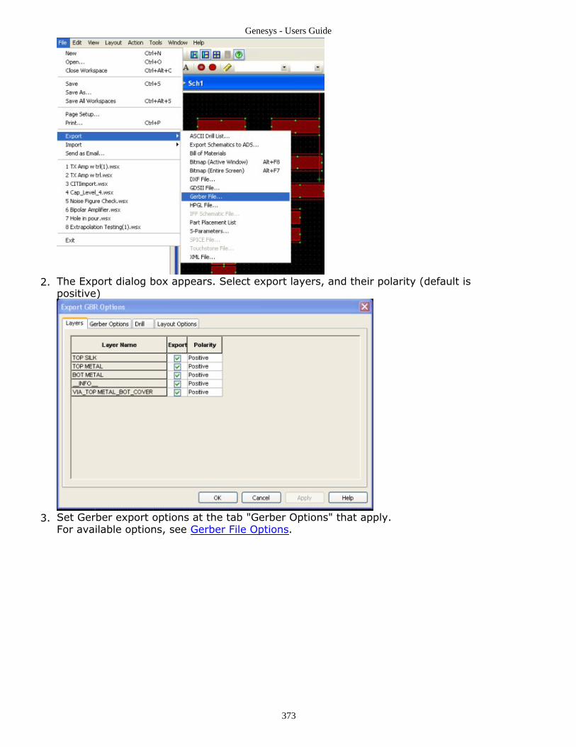
Genesys - Users Guide
373
The Export dialog box appears. Select export layers, and their polarity (default is2.positive)
Set Gerber export options at the tab "Gerber Options" that apply.3.For available options, see Gerber File Options.

Genesys - Users Guide
374
Drill file export is accomplished simultaneously as part of the Gerber export. The4.procedure for generating the drill file is similar to generating the Gerber file.To createGerber drill file, select exporting drill layers. You may edit actual drill tool diameterfor each drill hole.Note. All drill holes from the same the viahole layer are selected together.Drill files are configured from the Drill tab in the Export Gerber Options dialog.Selectthe check box to designate the layer for which you want to generate the drill file.When a layer is selected, all the tools on that layer are automatically selected. Bydefault, no drill file will be generated during Gerber export.The drill file options Number format, Output unit, and Zero suppression are same asoptions set for Gerber export in Options tab of Export Gerber Options dialog.However, note that the zero suppression in Drill is actually a zero inclusion.Tool Dia. (Diameter) is an editable field. By default the Tool Diameter value equalsthe Drawing Diameter value.
The exporting layout objects and output objects format may be specified at the5."Layout options" tab. It may include component footprints, EM-ports, and drill holes.All Genesys layout objects may be converted to "resolved" polygons by selecting"Convert all shapes into resolved polygons". In this mode you may specify layoutgeometry resolution parameters for arcs and linear layout object items.

Genesys - Users Guide
375
Click OK to save your settings or Cancel to retain the default settings.6.It closes "Export GBR Options" dialog and opens "Export GBR" dialog, setting outputGerber file(s) location.
As a default all output Gerber files will be exported in a single folder - one file perlayer(.gbr) and per drill layer(.drl).If it's exported to a single file - all Layout layers and drill holes will be saved in oneoutput Gerber file.Click OK to export the Genesys layout design to a Gerber file, or click Options to7.update export options.A Status window appears detailing the export information.

Genesys - Users Guide
376
If checkbox "View File after Export" is set, after the export it opens "Preproduction8.editor":
Gerber File Options
File format
Select RS274X for an enhanced version of Gerber RS274D format that supportsembedded apertures and G36/G37 polygons.Select MDA if your photoplot shop uses a FIRE 9000 plotter. It embeds aperturesand supports POEX/POIN polygons for fill on the fly.
Hole format
In Genesys, when a hole is created in a geometrical figure (like polygon), a cutline isintroduced. This is a false edge connecting the outer boundary of the polygon with theinner boundary. This polygon is actually a single re-entrant polygon. When you selectHoles as cutlines this re-entrant polygon is translated to Gerber as-is. The default isHoles as cutlines.
Holes as Cutlines
Select Holes as polygons or Preserve holes to remove the false edge from thepolygon.
Holes as polygons

Genesys - Users Guide
377
When Holes as polygons is selected, holes are exported as filled parts. Therefore thepolygon will appear to have no holes.
Preserve holes
When Preserve holes is selected, the resultant polygon in Gerber contains a dark areaand empty area. This option is not available for exporting Gerber files in RS274X format.
Unit
Available units are inch or mm. Inch is the default.
Number format
The number of integers placed before and after the decimal point. If chosen incorrectly,Gerber data resolution can be poor. The default is 2.4. If the unit is set to mm then youcan set the number format to 3.3.
A warning message is displayed in the Status window to notify the user that to preservethe precision in the Gerber data, number format has to be selected carefully. If the Gerberdata is not generated correctly for the selected number format then a suitable errormessage is displayed in the Status window.
Zero suppression
Available settings are Leading and None. Select Leading (the default) to remove allleading zeros in the coordinate data, making the Gerber file smaller.
Line width for polylines
Polylines in Genesys have zero width, but you can use this option to provide a width to beused for drawing this polyline in the Gerber file.
If the polylines and arcs (both zero width entities) are not required to be exported, thenset the width to zero.
Generate single file

Genesys - Users Guide
378
When this check box is selected, a single file is generated for all the selected layers in theLayer tab. Specify the file name with extension .gbr. This file will be created in thedestination directory selected in the Export dialog box.
Gerber Layer Options
All the layers used in the design are displayed in a table in the Layers tab of the ExportGerber Options dialog. By default, all the layers will be displayed with positive polarity andall layers will be exported. You can avoid exporting a specific layer by de-selecting thecheck box in the Export column for that layer.
Limitations and Considerations
No intermediate mask file is generated.The new Gerber export tool is targeted for the raster photoplotters to generateRS274X and MDA file format.No aperture filling is supported for polygons.No separate aperture file is required for RS274X and MDA files.You must set the appropriate number format in the Export Gerber Options dialog sothat the precision in Gerber data is more than the precision in layout design.The Gerber translator can generate a single Gerber file for all layers. However, theGerber Viewer cannot process a Gerber file in which multiple layers are defined in asingle file.It imports only the first layer defined in the file.Exporting MDA files using "Generate single file" option will export all the figures inthe same layer. It is advisable not to use "Generate single file" option for MDAformat. If a layer does not have any via (circles) then it will not be displayed in the Drill tableand no drill file will be generated for that layer.One drill file will be generated for each layer.Drill files will be created in the Destination directory selected in the Export dialog.Drill file name is the same as layer name with extension .drl. For example, drill filefor the layer cond will be cond.drl.If Tool Diameter is set to 0.0, the Tool Diameter will be equal to the DrawingDiameter in the output drill file.
Using the Pre-Production Editor
Genesys includes an editor that can display DXF/DWG and Gerber/Drill designs. Using theeditor, you can compare the DXF/DWG and Gerber/Drill files to the original Genesys layoutdesign to verify that the design was exported correctly. Similarly, DXF/DWG andGerber/Drill files can be previewed prior to import into Genesys:
to edit a large design down to a smaller design prior to importing it into Genesys.This edited design can be saved and then imported in Genesys.or after import, to verify that the DXF/DWG and Gerber/Drill design data and theGenesys-imported design appear similar.

Genesys - Users Guide
379
File Menu
The File menu contains common Open, Save, Save As, and Close functions and lists thefour most recent files viewed in the editor.
NoteWhen files are saved as Gerber/Drill files using the Pre-Production editor, the layer name is used as thefile name.
Edit Menu
The Edit menu contains common and specialized editing commands.

Genesys - Users Guide
380
EnableEditing
Enables editing commands to be performed on the current design. De-select this item to view thedesign in read-only mode. In this mode, editing commands are unavailable.
Undo Undoes the last editing command. A stack of edit commands is created enabling you to chooseUndo repeatedly to return to an earlier state of your design. A stack is maintained for eachwindow, thus the Undo command works independently from window to window.
Redo Returns the file to the pre-undo state.
Cut Enables you to delete one or more items from one window, and paste in another window.
Copy Enables you to copy items in a given design window and then paste those items within the samedesign window or another design window.
Paste Enables you to paste items that you previously cut or copied. You are prompted to enter the X andY coordinates of the position where you want to paste the copied items. Select Apply to paste orCancel to dismiss pasting.
Delete To delete selected items, click the Delete button on the toolbar, or press the Delete key on thekeyboard, or choose Delete from the Edit menu. Deleted items can be restored using the Undocommand.
Select All Enables you to select all figure(s).
DeselectAll
Deselects all the selected figure.
Modify This choice lets you modify the following items:
Select figures and click Union to perform union of the figures.Select figures and click Intersection to perform union of the figures.Select figures and click Union Minus Intersection to perform union of the figuresSelect Crop to crop an area from a figure(s).Select Chop to chop an area from a figure.
NoteUnion, Intersection, Union Minus Intersection, Crop, and Chop do not work for open ended figures withzero width (for example arc and polylines).
View Menu
The view menu contains commands that allow you to alter the view of the current design.
View All Your design is scaled and repositioned to fit within the viewing area.
The ZoomCommands
The Zoom commands enable you to enlarge or shrink the area being viewed. You can zoom inand zoom out using mouse wheel. The enlarged or condensed figure is moved towards thecenter of the window.
Zoom To Area > click a point and then with the mouse button pressed move the mouseto the bottom right of the area and release the mouse button to define a new view.Zoom to Point to zoom in on a specified point in the window. Click to specify a point andthe current view is magnified by a factor of two, moving the point you specify to thecenter of the window.Zoom In By 2 to zoom in by a factor of 2.Zoom Out By 2 to zoom out by a factor of 2.
Measure
The Measure dialog allows you to measure lengths.

Genesys - Users Guide
381
Absolute X, Y displays the absolute coordinates of the point of mouse click.Delta X, Y gives the relative X and Y coordinates from previous mouse click.Angle gives the angle with respect to a line horizontal to the X axis.Cumulative distance gives the total length from starting point to current point.Click Clear to reset the values for Absolute X,Y, Delta X, Y, Angle and Cumulativedistance.Click Cancel to dismiss the measure dialog box.
Undo/RedoStack
Shows last performed actions. You have an option to undo or redo the last operationsperformed.
Layer Table
The layer Table displays the layer information. It enables you to switch on/off layers fromdisplay. It also enables you to view layer number, layer name and layer color. Click Select Allto view all the layers and Deselect All to switch off all the layers. All the layers are displayedby default.
Status The status window displays messages about the status of the current design, as well as warningand error messages.
Window Menu
This menu contains the following common Window commands:
Close to close the active window.
Close All to close all open designs.
Tile to arrange all child windows in a tile pattern.
Cascade to arrange all the child windows in a cascade pattern.
Arrange Icons to arrange all iconified windows at the bottom of theworkspace.
Next to navigate to next open window.
Previous to navigate to previous open window.
Viewing Files in the Pre-Production Editor During Export
To view a DXF/DWG or Gerber/Drill file during export from Genesys:

Genesys - Users Guide
382
Select DXF/DWG or Gerber/Drill from File type drop-down list in Export dialog.1.Select the View file after export checkbox and click OK.2.This will display the exported DXF/DWG or Gerber/Drill file. A status window shows ifthe export is complete or failed and the design is displayed in the Pre-ProductionEditor.
Viewing Files in the Pre-Production Editor During Import
To view a DXF/DWG or Gerber/Drill file during import to Genesys:
Select DXF/DWG or Gerber/Drill from File type drop-down list in Import dialog.1.Click Preview to view the file in the Pre-Production Editor.2.
Editing Files in the Pre-Production Editor
Using the Pre-Production Editor you can cut, copy, paste and modify designs. From theModify menu, you can perform editing functions like union, intersection, union minusintersection, crop, and chop.
To edit using the Pre-Production Editor:
Open a design in the Pre-Production Editor as described above.1.Click Edit > Edit Enable.2.
To cut a figure, select the figure and then click Edit > Cut.To copy a figure, select the figure and then click Edit > Copy.
To crop or chop a figure:3.Select the figure.
Click Crop or Chop.Mark the area to crop/chop using mouse.

Genesys - Users Guide
383
Release the mouse to crop/chop the selected area.
Click Delete to delete selected item.4.Click Undo to revoke last Edit command.5.
Using Files From Earlier Genesys VersionsGenesys lets you load files created using all versions of Genesys prior to the currentversion. Once you save the files using the current version of Genesys, the files will notload in versions prior to GENESYS2005 (forward compatibility, and not backwardcompatibility).
GENESYS2005 and beyond are backward compatible as long as you disable Compact DataFormat (Tools / Options).

Genesys - Users Guide
384
Old Support:
Genesys imports files created using SUPERSTAR version 4 or later and any version ofGenesys. You cannot import the following features from versions of SUPERSTAR createdprior to version 4:
Post Processing - Genesys now has better post processing capability that is notcompatible with the old technique. For information on the new post processingprocedures, see the Simulation manual and the Using Equations chapter of the User'sGuide . Also, see the Genesys example file Model Extract.wsx.3D Graphs - Parameter sweeps are now different, so you must recreate 3D graphsafter importing them.EMPOWER Simulation Data - EMPOWER calculated data is now stored inside theworkspace file, instead of separate files. You must recalculate the data afterimporting. Also, you might want to set up any decomposition examples again,because Genesys version 7 and later provides better ways to set up these files. Formore information, see the EMPOWER manual.Multiple Impedances - Files with multiple WINDOW blocks reusing the samenetwork to simulate different terminations use only the first set of terminations.Impedances are now stored in the ports and are tunable. If you still need multipleimpedances:
Load your schematic.1.Create other schematics using NET blocks so your schematic can use the2.terminations you want.
Microstrip Radial Stubs (MRS) (part) - There is a new radial stub model with onlyone port that was introduced in Genesys version 7. Replace any radial stubs with amicrostrip tee and the new stub. For more information, see the part Catalog .
Using the ADS LinkGenesys provides a link to Advanced Design System (ADS). You can export schematicsfrom Genesys directly to an open ADS session by selecting File > Export > ExportSchematics to ADS. Genesys displays a dialog box showing all instances of ADS with openprojects.
You first select the instance that you want (if there is more than one running), then youselect which design/s to export to ADS. When you click OK, the selected schematics are

Genesys - Users Guide
385
transferred to ADS. See ADS RF Architect and Synthesis documentation (in theTransfer/IO section of the ADS documentation) for more information on using the link inADS.
The link transfers schematics only from Genesys to ADS. It does not transfer schematicsfrom ADS to Genesys. Only schematics and linear simulations will be transferred. Layouts,plots and datasets are not transferred. Not all schematics will transfer exactly, see ADSdocumentation for substrate/model mapping information.
Installation Requirements
An installed version of Genesys 2006.10 or newerAn installed Windows version of ADS 2006A or newer
Licensing
If Genesys was purchased as an ADS add-on, choose ADS style licensing in Genesys.On multi-CPU systems which use network licenses, it is important to always:
Stop the ADS simulator before launching Genesys.1.Exit Genesys before starting a simulation in ADS.2.
Accessing ADS Documentation
Documentation is available on the web at:http://edocs.soco.agilent.com/display/doc/Home ,or can be accessed by clicking a help button in ADS.

Genesys - Users Guide
386
LayoutsLayout creates a board description for sending to a board plotter or for simulating the EMeffects using EMPOWER simulation. You can export the layout for milling or etching instandard industry formats such as GERBER, DXF, and GDSII. You can also create a layoutfrom scratch.
ContentsCreating Layouts (users)Changing Layout Properties (users)Manipulating Layouts (users)Changing an Association Table (users)Adding Text and Changing Fonts (users)Reviewing Nodes and Rubber Band Lines (users)Using Layers (users)Adding Footprints to Layouts (users)Using the Footprint Editor (users)Using Pads in Layouts (users)Adding Polygons, Pours, and Ground Planes (users)Importing and Exporting Layout Files (users)Using Gerber Files (users)
Creating LayoutsA layout is the physical arrangement of parts on a circuit board. It creates a boarddescription that you can send to a circuit board manufacturer or use to simulateelectromagnetic effects through MomentumGXF. You can export a layout for milling oretching in standard industry formats such as Gerber, DXF, and GDSII. You can create alayout based on a schematic, from scratch, or from artwork imported from a file.
You can create a layout from scratch or based on a schematic.
To create a design with a layout:
Click the New Item button ( ) on the Workspace Tree toolbar and select Add1.Layout from the Designs menu.Define the layout properties and click OK.2.

Genesys - Users Guide
387
Use the layout toolbar to add metal to the layout.3.To add parts to a layout, place them in the associated schematic.4.
To create a design with a layout based on a schematic:
Create a design with a schematic.1.Use the Part Selector to add parts to your schematic.2.Right-click the Schematic tab and select Add Layout.3.
Select a component and click the Change Footprint button ( ) on the Layout4.toolbar to change the footprint used for specific components. For example, changethe footprint used by a specific capacitor to a larger or smaller footprint.Move and rotate footprints to the positions you want.5.Place lines and arcs as required to connect footprints and resolve the rubber band6.lines.Place any other required objects, such as text, connectors, non-schematic footprints,7.and ground planes.Send the finished layout to a printer, plotter, or file.We can add a layout to our8.current design..
The layout is automatically generated and added to the design.
Note: As you edit the schematic or partlist and add or delete parts these changes are reflected in thelayout.

Genesys - Users Guide
388
Note: Layouts can be associated with more than one design. Check the layout properties and ensure youare using the correct design(s).
Advanced technique - multiple windows Select Window / New Window from themenu, then resize and rescale ( hint: use Ctrl+Home to maximize the parts ) theschematic to get this..
Note: Some edits made in one window will be reflected in the other window only when it is clicked (toreduce processing overhead).
Changing Layout Properties
Changing Layout General Properties
Use the Layout Properties General page to change the general properties of a layout.
To change the general properties of a layout:
Click Layout on the Genesys menu and select Layout Properties.Click the General tab.Make the changes you want.Click OK.

Genesys - Users Guide
389
Designs to Include - This grid shows all available designs to place on the layout. Ifa box is checked, the layout will contain footprints and rubber band linescorresponding to the parts in that design. These footprints and rubber-bands willautomatically update as needed.Drawing Style - This is the fill mode for all metal filled objects (lines, rectangles,polygons, etc).
Solid Drawing Mode - Classic opaque fill."X-Ray" Drawing Mode - Semi-Transparent fill that allows users to seeoverlapping layers.Hollow Drawing Mode - Emphasizes edges, with a faint interior fill.
Units - The available units for dimensioning objects on the layout. If you enter anumber for a custom unit, simply use a constant multiplier for converting the unit tomillimeters. Some common numbers are:mm 1
mils .0254
meters 1000
inches 25.4
Object Dimensions - Default sizes for most commonly used objects. These numbersdefine the default dimensions line and pad widths, and the drill diameter for viaholes.Box Settings - Determines how the page is displayed on the layout screen. You canuse the page as a board edge indicator, for use in placing the footprints. This boxalso corresponds to the EMPOWER box. The following options are available:
Widths - The available widths for lines and arcs. The widths shown here areavailable in the Line Width combo box on the main LAYOUT screen.Remove - Removes the selected width from the Widths box (see above).Add New - Adds a new width to the available list in the Widths box (see above).Grid Spacing - The on-screen vertical and horizontal grid spacing, using theselected units. Parts are placed on this grid by default, so this numberdetermines the resolution for part placements.Grid Spacing X, Grid Spacing Y - These control the cell size for the EMPOWERrun as well as the grid snap feature in LAYOUT. When using the EMPOWER GridStyle, there will be LAYOUT snap points between each grid line which allow linesto be centered between two grid points if necessary. They are often referred toas dx and dy and should be small with respect to a wavelength at the maximumfrequency to be analyzed, preferably less than l/20 and always less than l/10.These parameters correspond directly to the DELTA statement in the TPL file.Show EMPOWER Grid - Turning on this check box forces LAYOUT to displaythe rectangular EMPOWER grid. It also allows different grid spacings in the X

Genesys - Users Guide
390
and Y dimensions. It is strongly recommended to turn this check box onwhenever you are creating a layout for EMPOWER.
Box Width (X,Y) - The desired width and height of both the page and thesurrounding EM analysis box, using the units selected in the Units box.Origin - The origin for mouse cursor measurements. The on-screen coordinatesdisplay information relative to this origin. The absolute origin is at the lower leftof the page. To specify a new origin, enter coordinates relative to the absoluteorigin, using the selected units. For example, if your page is 100 x 200 mils andyou want the origin at the upper left, you would enter 0, 100.Show Box (Check box) - Shows or hides the page boundary.Show Grid Dots (Check box) - Shows or hides the part placement grid.
Drawing Options - The following options are available:Port Size - The size (using the current units) for drawing ports.Rotation Snap Angle - The incremental angle (in degrees) used for rotatingobjects. This can be any number, but should be positive and < 360.Multi Place Parts (Check box) - Turns on or off multiple placement. In themain LAYOUT window, you click an object button (such as the Line button), toplace an object on the layout. Normally, the object button must be selectedevery time the object is to be placed. The Multi Place Parts option allows you toplace as many parts as you like by selecting the object button only once. PressEscape when done placing parts.Default Viahole Layers - The Start Layer and End Layer combo boxes controlthe default layers for the viaholes. These layers can be overridden individuallyfor each viahole if necessary. Currently, viaholes in EMPOWER can only go fromthe metal layer through one substrate layer to either the top or bottom cover.
Changing Layout Layer Properties
Use the Layout Properties Layer page to make changes to any of the layers in a layout.To change the general layer properties of a layout:
Click Layout on the Genesysmenu and select Layout Properties.1.Click the General Layer tab.2.Use the Show Columns check-boxes at the top to control which cells are displayed3.in the information grid.Make the changes you want.4.Click OK.5.
Name - The name assigned to each layer. This name is used throughout the programto identify the layer. Although you can type anything for the layer name, you should

Genesys - Users Guide
391
limit the length to about 12 characters, since combo boxes within the program arenot wide enough to display lengthy names.# - Layer numberColor - Shows the selected color for each layer. Click the button for any layer toselect another color.Layer Type - Identifies the layer type. Available options are:
None - This layer is considered blank (it is not used).Metal - All conductive traces and pads go on a metal layer.Substrate - Separates metal layers, and is used to indicate board dimensions.Any cuts or holes in the board (screw holes, etc.) go on a substrate layer.Silk - Silk screen is used for labeling on the final board. It is often white oryellow for easy identification.Mask (Solder Mask) - This is a negative layer - objects on this layer indicate anabsence of solder mask. This layer is automatically generated from pads andviaholes.
Note: Momentum will project mask layer objects onto the closest metal layer (ascopper).
Assembly - Indicates exact positions for component placement. It is used as adiagram for placing components at the production stage, and does not actuallyget used during board creation.Paste - Indicates where solder paste should be placed.
Hide - When selected, the corresponding layer is not shown in the layout.On Bottom (Mirrored) - When selected, the corresponding layer is mirrored (shownreversed) in the layout. This is useful for bottom layers, which would be reversedwhen viewing the top layer.Plot - Selects whether to plot the corresponding layer, when generating output(printing, exporting as Gerber, etc.)Etch Factor - Adds an etch factor to the corresponding layer, using the Layout units(mils, etc.) selected on the General tab.Use - Check this box to include the corresponding layer in the EM simulations(Momentum and/or Empower); uncheck it to omit the layer from EM simulations.Momentum-only Parameters:
Use Layer Mesh Density - When checked, Momentum will override its defaultlayer mesh density with the per-layer value specified in the next column on theright.Mesh Density - The mesh density, specified as an integer number of cells /wavelength; the default is 30.Use Layer TL Mesh - When checked, Momentum will override its default layertransmission line mesh setting with the per-layer value specified in the nextcolumn.TL Mesh - Transmission Line Mesh - An integer number of cells / width. 0 isautomatic.Edge Mesh - When checked, Momentum will override its default edge meshwidth setting with the per-layer value specified in the next column.Edge Mesh Width - The width of the edge mesh, using the Layout units (mils,etc.) selected on the General tab.Via Model
Default - Use the via setting specified in the Momentum GX analysis.Lumped - simulate the via using lumped parts.1D, 2D, 3D - Use 1 (wire), 2 (planar - no horizontal currents), or 3-dimentional (spacial - includes horizontal currents) simulation for the via.
Strip Model - not available when the layer is a "physical slot"Default - Use the strip model setting specified in the Momentum GXanalysis.2D, 3D - Use 2 or 3-dimensional simulation.

Genesys - Users Guide
392
Precedence - metal layer precedence for Momentum mesher (from 0 to 9,default = 0).
Type - Other entries in this table are different for each type of layer. To find help oneach column, see the section below for the type of layer: Top/Bottom Cover, AirAbove/Below, Metal, or Substrate layers.Top Cover & Bottom Cover - Describes the top and bottom covers (ground planes)of the circuit. Types include:
Lossless: The cover is ideal metal.Physical: The cover is lossy. These losses are described by Rho (resistivityrelative to copper). Momentum assumes a cover thickness of 0, while Empoweruses the Thickness and Surface Roughness parameters as well.Electrical: The cover is lossy and is described by an impedance or file. See thedescription below under metal for more information.Open: In Momentum, no cover will be simulated, also "Open" is not supportedin box simulation mode. In Empower (which always uses a box), the design issimulated as if the box walls and uppermost substrate/air layer extend up ordown forever (an infinite tube). In earlier versions of Genesys, this option wasknown as "Semi-Infinite Waveguide".Magnetic Wall: The cover is an ideal magnetic wall. This setting is only used inadvanced Empower (no Momentum) applications.Substrates: Choosing a substrate causes the cover to get the rho, thickness,and roughness parameters from that substrate definition. We recommend usingthis setting whenever possible so that parameters do not need to be duplicatedbetween substrates and layouts. Momentum ignores Thickness and SurfaceRoughness. For cover it always uses 0 thickness.
Air Above & Air Below - The presence of air at the top of the box (as in microstrip)or the bottom of the box (as in suspended microstrip) is so common that specialentries have been provided for these cases. Checking the box to turn these layers onis the equivalent of adding a substrate layer with Er=1, Ur=1, and Height (in unitsspecified in the Dimensions tab) as specified. For "Open" cover the Height of thecover air is ignored, when the other Air dielectric parameters (Er, Ur, Tand) definethe free space dielectric parameters.
Caution: When setting up a new circuit, be sure to check the height of the air above, as it is oftenthe only parameter on this tab which must be changed, and is therefore easily forgotten.
Metal Layers - Metal layers are used for metal and other conductive material suchas resistive film. The following types are available:
Lossless: The layer is ideal metal.Physical: The layer is lossy. These losses are described by Rho (resistivityrelative to copper), Thickness, and Surface Roughness.Electrical: The layer is lossy and is described by an impedance or file. This typeis commonly used for resistive films and superconductors. If the entry in thisbox is a number, it specifies the impedance of the material in ohms per square.If the entry in this box is a filename, it specifies the name of a one-port data filewhich contains impedance data versus frequency. This data file will beinterpolated/extrapolated as necessary. See the Device Data section for adescription of one-port data files.Substrates: Choosing a substrate causes the layer to get the rho, thickness,and roughness parameters from that substrate definition. We recommend usingthis setting whenever possible so that parameters do not need to be duplicatedbetween substrates and layouts.
Caution: Unless thick metal is selected, thickness is only used for calculation of losses. It isnot otherwise used, and all strips are calculated as if they are infinitely thin.
Metal layers have additional settings available:

Genesys - Users Guide
393
Metal Thickness - Thickness of the metal layer on a substrate.Rho - "Resistivity (relative to copper) is usually 1.0.Current Direction - Specifies which direction the current flows in this layer. Thedefault is along X and Y. "X Only" and "Y Only" can be used to save times on longstretches of uniform lines. "Z Up", "Z Down", "XYZ Up", and "XYZ Down" allow thecreation of thick metal going up/down to the next level or cover.Thick Metal - Checking this box instructs the EM analysis to model the metalincluding thickness. Empower does this by putting two metal layers close together,duplicating the traces on each, and connecting them with z-directed currents. If thickmetal is used, then Current Direction is ignored.Part Z-Ports - Specifies the default direction for automatically created part ports,either to the level above or to the level below. Generally, you should choose theelectrically shortest path for this direction.Physical Slot - Slot Type - In Momentum, if the Momentum Slot-Type combo-boxis set to "Slot", check this box to swap the metal and non-metal areas of the metallayer. (In Strip mode, this setting is ignored). In Empower, check this box tosimulate the non-lossless-metal areas (as opposed to the metal areas). Use this forground-planes and other layers which are primarily metal. Do not use this for lossylayers. See your Empower manual for details.Rough - Check this box to specify metal roughness in Empower. (This field is ignoredby Momentum.)Substrate Layers - These layers are used for substrate and other continuousmaterials such as absorbers inside the top cover. An unlimited number ofsubstrate/media layers can be used. The following types are available:
Physical w/Tand: The layer is lossy. The layer is described by Height (in unitsspecified in the Dimensions tab), Er (relative dielectric constant), Ur (relativepermittivity constant, normally 1), and Tand (Loss Tangent).Physical w/Sigma: The layer is lossy. The layer is described by Height (inunits specified in the Dimensions tab), Er (relative dielectric constant), Ur(relative permittivity constant, normally 1), and Sigma (Bulk Conductivity).Substrates: Choosing a predefined Substrate causes the cover to get theheight, Er, Ur, and Tand parameters from that substrate definition. Werecommend using this setting whenever possible so that parameters do notneed to be duplicated between schematics and layouts.
Caution: For true stripline (triplate), be sure to check the Use 1/2 Height check box if youare using a Substrate. This forces Empower to use 1/2 of the Substrate height for eachsubstrate (above and below) so that the total height for both media layers is correct.
Substrate layers have additional settings available:
1/2 Height - If the layout is a stripline circuit and is using a named substrate,checking this box forces Empower to use 1/2 of the Substrate height for eachsubstrate (above and below) so that the total height for both media layers is correct.Height - Height (thickness) of the substrate.Er - The "relative dielectric constant quantifies a material's ability to store chargewhen used as a capacitor dielectric, which affects the properties of transmission lines.The higher the constant the higher the energy stored within the capacitor. Er isdefined as the ratio of a material's capacitance to the capacitance of air. (Air = 1.0)Tand / Sigma - Tand and Sigma share the same column, since the parameters aremutually exclusive. Tand - the "dielectric loss tangent - is defined as the real part ofrelative permittivity / the Imaginary part of the relative permittivity. Sigma is thedielectric "Bulk Conductivity" value.Ur - The Relative Permeability of the substrate is also know as the magnetic constantis usually 1.0.

Genesys - Users Guide
394
Surface Impedance Value or File - The impedance of the surface of the substrateOR the name of a file Empower (only) to use instead. This field is only available formetal and covers, when Type is set to Electrical.Momentum Slot-Type - This setting affects any layer with a check mark in thePhysical Slot column. The combo-box has two choices, which indicate howMomentum should analyze the layout.
Strip - Momentum will interpret metal layers with "Physical slot" checked justlike Empower, i.e. without swapping the layer's metal and non-metal areas. Thisallows for the creation of layouts which are compatible with both Empower andMomentum: Empower never swaps metal with non-metal areas in the "physicalslot" metal layers - it simulates "Slot" layers internally.Slot - Each layer's "Physical slot" check box indicates that Momentum shouldswap its metal and non-metal areas. (Momentum changes the slot layertopology of the layout).
Insert Layer - Inserts a new layer at the current cursor position.Delete Layer - Deletes the layer at the current cursor position.Up / Down - Moves a layer up (or down) in the layer stack.Show / Hide All - Shows or hides all the layers (by checking all the check-boxes inthe Hide column).Use All / Use None - Checks all the "Use" column check-boxes, which indicateswhich layers will be simulated by Momentum or Empower.Load From Layer File - Loads a new layer configuration from a file. Save To Layer File - Saves the current layer configuration to a new file. Currently,only general and color info is retained (no Momentum, EM, or Empower layer data issaved).
Changing Layout Associations Properties
Use the Layout Properties Associations page to determine which footprint to initially usefor each type of design part using the Association table. The Association table is generallymodified only when a new layout is created. It is automatically saved using the currentname when you close the window, or you can save the table to a new name. You can alsoload a previously saved table.
Note: You must save the .TBL file into the {product-name}\LIB subdirectory. You cannot use theAssociation table if it is saved into other directories.

Genesys - Users Guide
395
Part Type - The category of parts for which footprints are loaded.Default Footprint - The footprint which is selected for the corresponding category(given in the Name column).Library - The name of the library containing the footprint for the correspondingcategory (given in the Name column).Change Button - Allows you to select a new footprint for the corresponding category(given in the Name column).Current Table - The file name of the current footprint association table.Save Table As Button - Saves the current table into a new file.Load Table Button - Loads a different footprint association table from a file.
To modify an entry in the Association table:
Click Layout on the Genesysmenu and select Layout Properties.1.Click the Associations tab.2.Scroll the table to find the entry you want.3.
Click the Change button to open the Choose Footprint Library window.1.Click a footprint library in the Select Library box.2.Click a footprint in the Available Footprints box.3.Click OK.4.
To save the Association table to a new file:
Click Layout on the Genesysmenu and select Layout Properties.1.Click the Associations tab.2.Click the Save Table As button.3.Type a name in the File Name box.4.Click Save.5.
To open a previously saved Association table:
Click Layout on the Genesysmenu and select Layout Properties.1.Click the Associations tab.2.Click the Load Table button.3.
Note: If the current table is already modified, a message asks whether to save the current table.Click Yes to continue.
Type a name in the File Name box.1.Click Open.2.
Changing Layout Font Properties
Use the Layout Properties Fonts page to change the default font properties for a layout.You can change only the font type and size. If you want to change the individual text in alayout, use the Text Properties window.To change the default font properties of a layout:
Click Layout on the Genesysmenu and select Layout Properties.1.Click the Fonts tab.2.Click a font in the Choose New Default Font box.3.Type a font size in the Default Size box.4.Click OK.5.

Genesys - Users Guide
396
Choose New Default Font - Lists the available fonts. The default font isautomatically selected when the dialog is opened. To choose a new default font,simply select another font in this box. All text already placed on the layout will beupdated to incorporate the new font. For a description of each font, please refer toReviewing Layout Fonts (users).Old Default - The old default font. If you have not selected a new font since openingthe dialog, this font stays selected in the Choose New Font box. This font will remainthe default style if you select Cancel on the dialog, even if you have selected another.Default Size - This is the default size for text placed on the layout. Changing thisnumber will update any text already on the layout that has the Use Default Size boxchecked in its properties box.
Manipulating LayoutsObjects in a layout are manipulated much like objects in any modern drafting or drawingprogram. Features like selecting objects, dragging, using object handles, grouping, andpanning are included.
Changing Object Properties
Object properties windows are used to adjust any properties of an object. These windoware especially useful when you must enter exact coordinates for objects. They appearautomatically during construction of ports, text, viaholes, and pads.To change object properties:
Double-click any of the following objects in a Layout window:1.ARCComponentEM PortGroupLinePadPolygonPortPourRectangleText

Genesys - Users Guide
397
ViaholeMake the changes you want.2.Click OK.3.
Selecting Objects
Generally, you must select objects before you can manipulate them. Objects change colorwhen selected.To select an object:
Click the Select button ( ) on the Layout toolbar. This button indicates that no1.object is currently being constructed.Click the object you want to select.2.
To select multiple objects:
Click the Select button ( ) on the Layout toolbar.1.Drag the mouse until a box is drawn completely around the items you want selected.2.
Note: The window pans automatically if you drag the mouse off thelayout.
To individually select multiple objects:
Click the Select button ( ) on the Layout toolbar.1.Hold down the Shift key while clicking each object. Other selected objects remain2.selected.
To select all objects:
Click Edit on the Genesys menu and select All from the Select menu. All the objects1.in the layout are selected.
To select an object hidden behind other objects:
Click the Select button ( ) on the Layout toolbar.1.Click where the object should be. If several objects overlap, continue clicking in the2.same spot until the object is selected. The layout cycles through the overlappedobjects with each click. Do not click too fast (double-click) because the object'sproperties window might appear.
Note: Another method of finding hidden objects is to use the X-ray mode. This makes the partssemi-transparent. You can find this option by using the General tab in the Layout Properties window.
Grouping and Ungrouping Objects
With the exception of port objects, you can combine objects into groups. This keepsobjects together as you move or rotate them. You can also nest groups so that one groupcontains other groups. When objects are grouped, there is no change to the final outputgenerated by the layout.Whenever any part of a group is selected, the entire group is selected. If you want toungroup parts after they are grouped, you must break apart the entire group.To group two or more objects:

Genesys - Users Guide
398
Select the objects you want to group.1.
Click the Group Objects button ( ) on the Layout toolbar.2.
To ungroup previously grouped objects:
Select the group you want to ungroup.1.
Click the Ungroup button ( ) on the Layout toolbar.2.
Converting a Component to a Group
When a component is placed in a layout, you can make only simple changes to it:
Move, rotate, or move the component to a new layer.Change or remove text.Move text using object handles.Hide the silk screen using the Component Properties window.
If you need to make other changes to the object, use the Footprint editor. However, if thechange is unique, such as removing unused pins from an edge connector, make thechange in the Layout window by first converting the component to a group.To convert a component to a group:
Click the Component Footprint button ( ) on the Layout toolbar to place the1.component if it is not already in the layout.Select the component you want to group.2.
Click the Group Objects button ( ) on the toolbar.3.
Note: If a message appears stating you cannot change the object to a group because it hasassociated schematic parts, follow the instructions in the Deleting Objects section to remove thelink.
Using Object Handles
You can modify objects in various ways using object handles. Object handles are smallsquares that appear when an object is selected. You can manipulate object handles onlywith a mouse.
Note: There is a limited ability to manipulate objects if there is an associated schematicpart.
On rare occasions, you might want to manipulate object handles without snapping to thegrid, nodes, or a specific angle. Be aware that when doing so, it is easy to break electricalconnections or to rotate parts to nonstandard angles, so only do so when necessary. Touse an object handle:
Select the objects you want to move.1.Drag an object handle to manipulate the object. An outline image updates as changes2.are made.
Note: The window pans automatically if you drag the mouse off thelayout.
To use an object handle without snapping to grid, nodes, or angles:

Genesys - Users Guide
399
Select the objects you want to move.1.Hold down the Shift key and drag an object handle to manipulate the object. An2.outline image updates as changes are made.
Note: The window pans automatically if you drag the mouse off thelayout.
Moving Objects
Often, you must move objects to complete a layout. In addition, on rare occasions, youmight want to move objects to a point not on the grid.
Caution: It is easy to break electrical connections, so please move objects to a point not on the grid onlywhen absolutely necessary.
To move an object:
Select the object you want to move.1.Drag the mouse until the outlined image is in the location you want. Do not drag2.using an object handle. The image snaps to the grid.
Note: The window pans automatically if you drag the mouse off thelayout.
To move an object without snapping to grid or nodes:
Select the object you want to move.1.Hold down the Ctrl key and drag the mouse until the outlined image is in the location2.you want. Do not drag using an object handle.
Cutting, Copying, and Pasting Objects
You can cut, copy, or paste layout objects. When you cut an object, you remove it fromthe layout. Copying an object leaves the object in the layout. Once cut or copied to thebuffer, you can paste duplicates of objects back to the layout.
Note: You cannot cut objects associated with schematic parts. If a message appears stating that youcannot cut an object because it has associated schematic parts, use copy instead.
Cutting and pasting objects allows for the easy duplication of objects. The layoutremembers the last cut or copied object until you exit Genesys. Only one cut or pastebuffer is used for both the standard Layout editor and the Footprint editor, allowing you tocut and paste objects between them. You can paste as many duplicates as you want.Duplicates are always pasted to the same place as the original objects. You can movethem to a different location.
CAUTION: The contents of the cut and paste buffer are lost when you exit Genesys.
To cut an object:
Select the object you want to cut.1.Click Edit on the Genesys menu and select Cut.2.
To copy an object:
Select the object you want to copy.1.

Genesys - Users Guide
400
Click Edit on the Genesys menu and select Copy.2.
To paste duplicates of the last object cut or copied:
Click Edit on the Genesys menu and select Paste.1.Move the object to the location you want.2.
Note: Objects you paste are not associated with schematic parts even if the original objects haveassociated schematic parts.
Connecting Layout Parts Automatically
A layout can automatically snap parts together. This is very useful for microstrip andstripline circuits that have parts automatically created from a schematic (such as filesfrom M/FILTER). For example, in two easy steps you can turn this layout:
into this layout:
To automatically connect objects:
Select the objects you want to connect.1.Click Layout on the Genesys menu and select Connect Selected Parts.2.
Adding Lines, Rectangles, and Arcs
Lines and arcs are typically used to make electrical connections. In layouts strictly forEMPOWER, you should turn off the round ends for these lines and arcs. For most otherpurposes, you should use round ends, because they make better connections. Also, inlayouts for EMPOWER, you might find it easier to use rectangular objects for mostpurposes.Using the Layout toolbar, you can set round or square ends, width, and layer informationfor lines and arcs. You can also make lines orthogonal (90 degrees) using the Layouttoolbar or the Line properties window.To draw a straight line:
Click the Line button ( ) on the Layout toolbar.1.

Genesys - Users Guide
401
Click in the layout at the starting point of the line.2.Drag your mouse to the ending point of the line.3.
To draw two connected orthogonal (90 °) lines:
Click the Line button ( ) on the Layout toolbar and draw a straight line.1.Draw a second line perpendicular to the first line and connect one end of the second2.line to one end of the second line (green dots).Click one of the lines.3.Press the O key to convert the line to two orthogonal segments.4.Press the F key to flip the orthogonal direction, if necessary.5.
To draw a rectangle:
Click the Rectangle button ( ) on the Layout toolbar.1.Click in the layout where you want the upper-left corner of the rectangle.2.Drag the mouse to the lower-right corner of the rectangle.3.
To draw an arc:
Click the Arc button ( ) on the Layout toolbar.1.Click in the layout at the starting point of the arc.2.Drag your mouse to the ending point of the arc. You see a thin line between the3.starting point and the mouse position as you drag the mouse.Move the mouse to define the curvature of the arc.4.Click to finish drawing the arc.5.
Deleting Objects
When you delete objects from a layout, the objects are not placed into a buffer the sameas when you cut or copy objects. Deleting removes objects from the program, and youcannot paste deleted objects back into the layout.
Note: You cannot directly delete layout objects with associated schematic parts. Instead, you must eitherdelete the part from the schematic, remove the schematic from the layout, or set the schematic object tonot include a layout object.
To delete layout objects:
Select the object you want to delete.1.Click Edit on the Genesys menu and select Delete.2.
To remove a schematic from a layout:
Click Layout on the Genesys menu and select Layout Properties.1.Click the General tab.2.Click the check box for your layout in the Designs to Include box.3.Click OK. All parts and rubber bands from the schematic are removed.4.
To remove a layout object with an associated schematic part:
Click Layout on the Genesys menu and select Layout Properties.1.Click the Schematic tab.2.Click the schematic part that corresponds to the layout part you want to delete.3.

Genesys - Users Guide
402
Double-click the part to open its properties window.4.Click the Layout button.5.Click either the Replace Part With Open or Replace Part With Short button.6.Click OK to close the Layout Options window.7.Click OK to close the properties window.8.
Changing an Association TableThe Association table is used whenever a new layout is created or any time a layout isupdated with new parts in the design. It is only used once for any given part. Associationtables are used by a layout to determine which footprint to initially use for each type ofdesign part. You can later change this footprint from within the layout to override theAssociation table.Whenever a file containing a layout that depends on a schematic is loaded, the date of theschematic file is checked against the date of its Association table. If the Association tableis newer than the schematic file, a message appears. This message is useful to helpensure that outdated footprints are not accidentally used in a layout.The following information helps clarify the use of an Association table:
A new schematic is created containing a capacitor, C1.A new layout is created. In the Association table, the entry for CAP shows the libraryname SM782.LIB, and the footprint shows the name CC1005 [0402] Chip Capacitor.This footprint is automatically placed in the layout for the capacitor.If the Association table is later changed, it has no effect on the capacitor that wasalready placed.If the footprint for the existing capacitor is changed (for example, to CC2012 [0805]Chip Capacitor), it is not automatically changed back to the Association table entry.Even if the schematic is modified, the capacitor does not automatically move orchange back to the Association table entry.If the schematic part is deleted, the corresponding part in the layout is deleted.If the Association table contains a multi-part footprint (such as a quad op-ampfootprint), all devices in each component is used before beginning a new one. Forexample, if a schematic contains seven op-amps and the OPA entry in the Associationtable contains a quad op-amp footprint, two components are placed. The firstcomponent uses all four devices, and the second component uses three of its fourdevices.
Changing the Component Footprints
Once a component is automatically generated for a schematic part, you can change itsfootprint. The component continues to use the new footprint even if the schematic ismodified.To change a component's footprint:
Select the component you want to change.1.
Click the Change Footprint button ( ) on the Layout toolbar to open the Choose2.Footprint Library window.Click a footprint library in the Select Library box.3.Click a footprint in the Available Footprints box.4.Click OK.5.
Adding Text and Changing FontsYou can add text to your layout to label objects or to convey information on silk layers.Included in Genesysis a variety of different fonts that you can use for text objects in alayout. You can also use your own TrueType font.

Genesys - Users Guide
403
Note: The text changes you make to a specific layout affect only the text in that layout. If you want tochange the default text font and size for all layouts, you must use the Layout Properties Font window.
Adding Text to Layouts
Once you add text to a layout, you can edit it, change the font, or change the size.To add text to a layout:
Click the Text button ( ) on the Layout toolbar.1.Click in the layout where you want to place text. The Text Properties window2.appears.Type the text in the Text box.3.Make any other changes you want.4.Click OK.5.
To change the text in an existing text object:
Select the text you want to edit.1.Click Edit on the Genesysmenu and select Parameters to open the Text Properties2.window.Edit the text in the Text box.3.Click OK.4.
To change the font used by an existing text object:
Select the text whose font you want to change.1.Click Edit on the Genesysmenu and select Parameters to open the Text Properties2.window.Select a font in the Font list.3.Click OK.4.
To change the size of an existing text object:
Select the text whose size you want to change.1.Click Edit on the Genesysmenu and select Parameters to open the Text Properties2.window.Clear the Use Default Size check box if it is selected.3.Type the new text size in the Text Size box. The size is given in the units specified in4.the General tab of the Layout Properties window.Click OK.5.
Changing the Default Text
Most text placed in a layout is associated with a footprint, and you cannot control the fontand size. However, you can change the default font and size, which changes the text forall other objects simultaneously. This process adjusts the font and size of all text objectsthat are marked (in their properties windows) to use the default font or the default size.This includes all text in footprints from libraries supplied with layouts.To change the default font and size:
Click Layout on the Genesysmenu and select Layout Properties.1.Click the Fonts tab.2.Click a font in the Choose New Default font list.3.Type a new size in the Default size box.4.

Genesys - Users Guide
404
Click OK.5.
Reviewing Layout Fonts
The provided fonts are all in Eagleware-Elanix font (.EWF) format, which is a proprietaryfont format. They are located in the Font subdirectory of the main Eagleware-Elanixdirectory (C:{product-name}\Font). If additional fonts are needed, you can copy TrueTypefonts (.TTF) into this directory, with the following constraints:
There are many different TrueType font formats available and not all are guaranteedto work in a layout.When text using a TrueType font is converted to Gerber format, each letter of thetext is converted into a filled polygon. Extremely large Gerber files result if TrueTypefonts are used extensively. TrueType fonts are best used for highlights and userinstructions, such as a company's name and logo or jumper settings. In contrast, thesize of text in a Gerber file using an .EWF font is roughly proportional to thecomplexity of the .EWF font.
Layout includes the following fonts (complexity directly relates to Gerber file size):
Font Description Complexity (1-10)
DEFAULT.EWF A thin font. This font is appropriate for use on most boards. 4
EURO.EWF A thin font that is somewhat boxier than DEFAULT.EWF. 4
GOTH.EWF A very artistic gothic font. 10
LCOM.EWF A font resembling Times Roman. This font is especially useful for placing alarge company name on a layout.
6
LITT.EWF A very simple thin font. This is the simplest provided font. 2
SANS.EWF A sans serif font of medium stroke thickness. 7
SCRI.EWF A thin ornamented font designed to resemble handwriting. 5
TRIP.EWF A bold font resembling Times Roman Bold. 9
TSCR.EWF A bold italic font resembling Times Roman Bold Italic. 9
Reviewing Nodes and Rubber Band LinesNodes (shown as green dots) are shown in a layout where you can make electricalconnections. Any objects placed or handles moved snap automatically to a nearby node toensure a true connection. These nodes allow consistent electrical connections even whenparts do not line up on a grid. (If you do not want to snap to the grid or to a node, holddown the Shift key while moving or constructing an object.)
Rubber band lines (shown as thin white lines) are shown in a layout where you can makeelectrical connections. These connections are determined from the designs. The rubberband lines update whenever the designs change. Rubber band lines disappearautomatically as connections are made.
Rubber band lines show only one possible set of connections. For example, figure (a)below shows three parts that can connect. The most obvious connection method is shownin figure (b). However, you do not need to follow the rubber band lines exactly. Theconnections in figure (c) also resolve the rubber bands because they electrically connectthe three nodes.

Genesys - Users Guide
405
You cannot use objects other than lines, arcs, or viaholes to resolve rubber bands. Forexample, if a polygon is placed between two nodes, those two nodes are not consideredconnected, even if the polygon appears to connect the two nodes.
Note: One cause of rubber band lines not disappearing is the failure to actually connect nodes together. Ifrubber bands do not disappear, zoom in and examine the nodes to ensure the connections are properlymade.
The automatic resolution, or removal, of rubber band lines is intelligent. You can use anycombination of lines, arcs, and viaholes to make connections. The layout resolves therubber bands properly no matter how complex the interconnections.
Tip: A common mistake is to use a fine grid, which allows components to look connected when theyactually have a small gap between them. This problem is often hard to find in large layouts, but you canensure that actual connections take place by keeping the grid spacing coarse.
Reviewing Rubber Band Resolutions
You can use the Statistics window (sometimes referred to as a scorecard) to review yourprogress resolving rubber bands. This window tells how many rubber bands there wereinitially and how many rubber bands are successfully resolved.To review your progress resolving rubber bands:
Click Layout on the Genesys menu and select Statistics.
Using LayersA layout recognizes six distinct layer types, which are considered a Layer table:
Metal – Used for all conductive traces. Only traces on metal layers are used toautomatically resolve rubber bands.Silk – Used for labels on the final board. It is generally white or yellow on theproduction board. Silk screen objects should not overlap with solder mask objects.Substrate – Used to designate cuts in the circuit board. If automatic cutting isemployed, you should use only straight or orthogonal rounded-end lines. The centerof these lines represents the saw path for cutting.Assembly – Used to indicate exact placement of components. This is anintermediate layer. It is only used as an aid in the production process and is not seenon the final board.Mask (Solder Mask) – Objects indicate an absence of solder mask. This is anegative layer. It is automatically generated from pads and viaholes and generallydoes not require user intervention.Paste (Solder Paste) – Objects indicate places to use solder paste. If a solder pastelayer is required, you must manually generate it.
Note: You can enter layer information using the Layer tab of the Layout Properties window.
Reviewing the Types of Layers

Genesys - Users Guide
406
A layout can deal with almost any board configuration, from a simple one-layer board to acomplex sixteen or more layer board. Mixed media, such as combining microstrip withstripline, are easily accommodated. There are up to 128 different layers to use, and youcan use each type as often as you want. Some possible layer setups are:For a simple, single-layer board or prototype with a solid ground plane (no traces orcutouts on the ground plane) (SIMPLE.LYR):
SilkMetal
For a typical single-layer production board (SINGLE.LYR):
Top AssemblyTop SilkTop MaskTop MetalSubstrateBottom Metal (Mirrored)Bottom Mask (Mirrored)Bottom Silk (Mirrored)Bottom Assembly (Mirrored)
For a four-layer production board (FOUR.LYR):
Top AssemblyTop SilkTop MaskTop MetalSubstrate 1Metal 2Substrate 2Metal 3Substrate 3Metal 4Substrate 4Bottom Metal (Mirrored)
Bottom Mask (Mirrored)Bottom Silk (Mirrored)Bottom Assembly (Mirrored)
Selecting a Drawing Style
Several drawing styles are available to facilitate the construction and manipulation ofobjects on various layers. The drawing styles are:
Solid (Opaque)X-ray ModeHollow
To select a drawing style:
Click Layout on the Genesys menu and select Layout Properties.1.Click the General tab.2.Click a button to indicate the drawing mode.3.

Genesys - Users Guide
407
Note: Use the hollow or x-ray modes to make all objects visible, regardless of thelayer.
Click OK.4.
Hiding Layers
Often it is necessary to turn off the display of certain layers. For example, if an assemblylayer is not being modified, you can hide it:To hide a layer:
Click Layout on the Genesys menu and select Layout Properties.1.Click the Layer tab.2.Scroll down to the layer you want.3.Click the check box in the Hide column.4.Click OK.5.
Mirroring Layers
Be sure to mirror layers on the back side of a board. For example, when viewing from thetop of the board, the lettering and component footprints are reversed. When a layer ismarked as mirrored, all future text and components placed on that layer are mirrored.To mark a layer as mirrored:
Click Layout on the Genesys menu and select Layout Properties.1.Click the Layer tab.2.Scroll down to the layer you want.3.Click the check box in the Mirror column.4.Click OK.5.
Using Layer Files
You can save layer setups into files for later use in other boards. Unlike Footprint libraryfiles, layer files (LYR) do not remain associated with a particular layout. If layer settingsare saved to an LYR file and the settings are later changed in the current layout, the LYRfile does not update automatically. If the LYR file is later changed, no layouts are changedunless the LYR file is explicitly loaded.To save layer settings into an LYR file:
Click Layout on the Genesys menu and select Layout Properties.1.Click the Layer tab.2.Click the Save to Layer File button.3.Type a name in the File Name box.4.Click Save.5.
To load layer settings from an LYR file:
Click Layout on the Genesys menu and select Layout Properties.1.Click the Layer tab.2.Click the Load from Layer File button.3.Type the name of the Layer file to load in the File Name box.4.Click Open.5.
Adding Footprints to LayoutsA footprint is a pattern of metal, silk, and other layers that generally corresponds to a

Genesys - Users Guide
408
physical part, such as SOT23 or 0603 packages. You can create or edit footprints usingthe Footprint editor and then save the footprints into a footprint library. If a footprintlibrary is changed, all components in all layouts using that footprint are changed. You canassociate footprints with parts using the Association table or by editing a part in the PartSelector to add a footprint property to the part.
Creating and Saving Footprints
You can create and save footprints to use in other layouts. Store the footprints in a libraryyou create.To create a new footprint:
Click Tools on the Genesys menu and select New Footprint from the Footprint1.Editor menu.Place objects in the Footprint editor.2.Place pads wherever you want to make solder connections.3.Place silk screen objects (for example, designators).4.Place ports. Always place ports before saving a footprint.5.Click Tools on the Genesys menu and select Save Footprint from the Footprint6.Editor menu to save the footprint in a library file.
To save an existing footprint:
Click Tools on the Genesys menu and select Save Footprint from the Footprint1.Editor menu.Click the library that contains the old footprint in the Select Library box.2.Click the footprint in the Available Footprints box.3.Click OK.4.
Warning: The old footprint is lost if this method is used to save because any layouts using the oldfootprint are modified. Use a new name if the old footprint is needed later.
To add a new footprint to an existing library:
Click Tools on the Genesys menu and select Save Footprint from the Footprint1.Editor menu.Click the library to add the footprint to in the Select Library box.2.Click <New Object> in the Available Footprints box.3.Click OK.4.Type a new name for the footprint in the box.5.Click OK.6.
To create a new library and save the current footprint into it:
Click Tools on the Genesys menu and select Save Footprint from the Footprint1.Editor menu.Click <New File> in the Select Library box.2.Ensure that <New Object> is selected in the Available Footprints box.3.Click OK.4.Type a name for the new library file in the File Name box, and then click Save.5.Type a new name for the footprint in the box.6.Click OK.7.
Creating Multi-Part Footprints

Genesys - Users Guide
409
Multi-part footprints (for example, bus resistors) are created by assigning port numbers todifferent parts within the footprint. The first part (schematic part) within the footprint isusually labeled part A. For example, the first resistor in a bus package is part A.The first pin of part A is labeled pin 1, so the port that designates the first pin of part A islabeled A1 on the footprint. This is shown in the Footprint Example 2 (users) section.
Using the Footprint Libraries
Four footprint libraries are included with a layout. You can use these libraries to addfootprints to your layouts. Certain footprints, such as 14-pin DIP packages, have hundredsof possible uses. They can be a quad op-amp or a multiple transistor package. Portassignments in these devices are sequential, such as pin 1 through 14. When you usesuch a device, you must create a specific footprint with different port numbering.You can create new footprints based on a footprint in one of these footprint libraries. Justload an existing footprint, modify it as necessary, save it with a new name, and store it ina new footprint library.
SM782.LIB - A library based on the IPC SM 782 surface mount standard(SM782.LIB). There footprints are from the Institute for Interconnecting andPackaging Electronic Circuits SM 782 standard, Revision A, August 1993. You cancontact IPC at 7380 N. Lincoln Ave., Lincolnwood, IL, 60646.This standard is very specific on dimensions for the landing patterns. In general,maximum dimensions are used in creating the library footprints.The silk screens are generated by Agilent based on general industry conventiondetermined by reviewing several PWBs.LEADED.LIB - A leaded component library (LEADED.LIB). These are leaded partfootprints. They are generated from data provided by the following manufacturers:Coilcraft, ITT, J.W. Millar, Kyocera AVX, Motorola, Murata, Panasonic, R-Ohm, andToko.The through holes in this library are typically 20 mils larger than the lead diameter,and the pads are 35 mils larger than the through hole diameter. In certain activedevices, such as DIP ICs and TO-92 transistors, sufficient spacing is not available andsmaller margins are used.The silk screens are generated by Agilent based on general industry conventiondetermined by reviewing several PWBs.HPLIB.LIB - A library of sample footprints (SAMPLE.LIB). These transistor footprintsare taken from the HP Communications Components GaAs & Si Products data book.SAMPLE.LIB - A small library of active RF devices (HPLIB.LIB). These miscellaneousleaded and surface mount footprints are for objects such as mounting screws,coplanar grounds, grounds with via holes, grounds with wagon wheel pads and asample quad operational amplifier.
Generating Transmission Lines Automatically
In typical digitally oriented PCB layout or CAD programs, you must manually generatetransmission lines and their junctions (discontinuities). This is often tedious, timeconsuming, and error prone.In contrast, a layout automatically generates footprints for microstrip and stripline partsentered in a schematic. The dimensions of these footprints are automatically determinedfrom the schematic parts and substrate parameters, ensuring that the board is laid outexactly as simulated. The table that follows lists [ part types|superstar_parts] that arehandled automatically by a layout (and, correspondingly, are not listed in the Associationtable).

Genesys - Users Guide
410
Part Type Description
Microstrip and stripline bends (MBN, SBN) A square or chamfered (triangular) polygon for the cornersection.
Microstrip and stripline single lines andcoupled lines (MCN, MCP, MLI, MTAPER, SLI,SCN, SCP)
Generates lines and spacings.
Microstrip cross and tee, and stripline tee(MCR, MTE, STE)
A square or rectangular polygon for the area where three orfour lines come together.
Microstrip curved line (MCURVE) A curved line is generated.
Microstrip inductors & capacitors (MIDCAP,MRIND, MSPIND)
Complex footprints representing these parts are generated.
Microstrip and stripline open end effects(MEN, SEN)
Have no size and are removed from the layout.
Microstrip and stripline gaps (MGA, SGA) Two small metal guide pieces separated by the gap width.
Microstrip radial stub (MRS) Generates a pie-shaped piece.
Microstrip and stripline steps (MST, SSP) Removed for symmetrical microstrip and stripline steps. Forasymmetrical microstrip, two guide pieces plus nodes aregenerated.
Microstrip viaholes (MVH) Generates a viahole with its pads.
Note: Be sure that the units given in the substrate are correct, because these are the units used forgenerating the microwave footprints. The units specified on the General tab of the Layout Propertieswindow are not used for this purpose.
When a layout containing these parts is created, footprints for these parts are generatedautomatically and are connected by rubber bands initially just like any other parts. Themain difference is that instead of connecting these parts with lines, they are normallymirrored, moved, and rotated until their nodes join, eliminating the rubber band lines. Youcan manually or automatically join these parts.To automatically join multiple microwave footprints:
Select the objects you want connected.1.Click Layout on the Genesys menu and select Connect Selected Parts.2.
To manually join together two microwave footprints:
Select the first object.1.
Click the Mirror button ( ) on the Layout toolbar if the first object must be2.mirrored.Use the object handles to rotate and move the object as necessary. For unusual3.positioning or rotation angles, use the Component Properties window.Select the second object.4.Click the Mirror button on the Layout toolbar if the second object must be mirrored.5.Use the object handles to rotate the object as necessary. For an unusual rotation6.angle, use the Component Properties window.A rubber band now connects a node onthe first object (node A) with a node on the second object (node B).Drag node B to node A. The two objects snap together, eliminating the rubber band.7.
Placing Component Objects
Component objects in a layout represent lumped parts, such as resistors, transistors, andintegrated circuits. You can also use component objects if a complex pattern needsrepeating in many layouts, such as connectors.All components are based on a footprint in a footprint library. If a footprint library ischanged, all components in all layouts using that footprint are changed.

Genesys - Users Guide
411
If a layout is based on one or more designs, components and rubber bands areautomatically placed corresponding to the design topologies. The General tab of theLayout Properties window controls which designs to include in the layout. You can usethe Association table to determine which footprint to use for each type of part. If anycomponents are added, modified, or deleted in the designs, the layout components andrubber bands are automatically added, modified, or deleted.To place a component object:
Click the Component Footprint button ( ) on the Layout toolbar.1.Click the library that contains the footprint in the Select Library box.2.Click the multi-part footprint in the Available Footprints box.3.Click OK.4.Click in the layout where you want to place the component.5.
Switching Parts in Multi-Part Footprints
Multi-part footprints such as resistor packs or quad op-amp integrated circuits (ICs) aresupported in a layout. You can move two or more individual parts with associatedschematic parts into a multi-part footprint.Sometimes, you might want to switch existing component associations. For example, ifthere are two quad op-amp packages in the layout, each with four associated schematicparts, you can change which part is associated with which part.To switch parts with associated schematic parts into a multi-part footprint:
Select the part you want to switch.1.
Click the Change Footprint button ( ) on the Layout toolbar.2.Select the desired multi-device footprint from the library window.3.Choose Switch/Move Parts from the Layout Menu. For the next several steps, help4.will appear on screen in the status bar.Select the next component to place into the multi-part package.5.Select the component with the multi-device footprint to place the second component6.into.A message will appear stating that the original component no longer is associated7.with any schematic parts and asking if the original part should be deleted. Normally,you will press the "Yes" button.Repeat steps five through seven for any remaining individual parts to place into the8.multi-part footprint.
Sometimes, you may want to switch existing component associations. For example, ifthere are two quad op-amp packages on the layout, each with four associated schematicparts, you may want to change which device is associated with which part.To switch schematic part associations between two component devices:
Choose Switch/Move Parts from the Layout Menu. For the next several steps, help1.will appear on screen in the status bar.Select the first component's device to switch. This component must have an2.associated schematic part.Select the multi-device footprint to switch with or move into.3.If a message appears stating that the original footprint no longer is associated with4.any schematic parts and asking if the original part should be deleted, you willnormally press he "Yes" button.

Genesys - Users Guide
412
Note: For information on modifying the Association table to use multi-part footprints, see theChanging the Associations Layout Properties (users) section. For information on changing thefootprint of an existing part, see the Changing Component Footprints (users) section.
Loading and Merging Footprints
To load an existing footprint:
Click Tools on the Genesys menu and select Load Footprint from the Footprint1.Editor menu.Click the library that contains the footprint in the Select Library box.2.Click the footprint in the Available Footprints box.3.Click OK to load the footprint.4.
To merge an existing footprint with the current footprint:
Click Tools on the Genesys menu and select Merge Footprint from the Footprint1.Editor menu.Click the library that contains the footprint in the Select Library box.2.Click the footprint in the Available Footprints box.3.Click OK to merge the footprint.4.
Renaming and Deleting Footprints
You can change the name of a footprint or delete a footprint if it is no longer needed.To rename a footprint:
Click Tools on the Genesys menu and select Modify Footprint Library from the1.Footprint Editor menu.Click the library that contains the footprint in the Select Library box.2.Click the footprint in the Available Footprints box.3.Click the Rename button.4.Type a new name for the footprint in the New Name box.5.Click OK.6.
To delete a footprint:
Click Tools on the Genesys menu and select Modify Footprint Library from the1.Footprint Editor menu.Click the library that contains the footprint in the Select Library box.2.Click the footprint in the Available Footprints box.3.Click the Delete button.4.
Using the Footprint EditorLayouts in Genesys also include an editor for creating and editing footprints and libraries.The figure below shows a Footprint Editor window.

Genesys - Users Guide
413
To open the Footprint editor:
Click Tools on the Genesys menu and select New Footprint from the FootprintEditor menu.
Reviewing Layers in the Footprint Editor
The following layers are available in the Footprint editor:
Top AssemblyTop SilkTop PasteTop MaskTop MetalSub AboveMetalSub BelowBottom MetalBottom MaskBottom PasteBottom SilkBottom Assembly
For almost all components, place pads on the metal layer and not the top metal layer.Place all silk screen objects on the top silk or bottom silk layers.
Note: If you might ever use your footprint on the back side of a board, you must place your pads on thebottom metal layer and not the top metal layer so that the layout automatically mirrors your pads andmoves the component to the back of the board.
Placing Objects in the Footprint Editor
Objects in the Footprint editor are placed exactly the same way that they are placed in theLayout window. Whenever you select an object, the Layout toolbar shows the availableoptions for that object. You can change any of these options before placing the object. Theavailable objects are listed on the toolbar at the top of the Footprint Editor window. Theyare as follows:
Lines ( )
Rectangles ( )
Arcs ( )

Genesys - Users Guide
414
Polygons ( )
EM Ports ( )
Text ( )
Viaholes ( )
Pads ( )
To place an object in the Footprint editor:
Click the appropriate button on the Layout toolbar.1.Click in the Footprint editor to place the object.2.
Note: If the object's properties window appears, specify the options you want and then click OK.
Placing Pads in the Footprint Editor
You should place pads wherever solder connections are made. Pads always have a node atthe center, regardless of the pad shape.To place a pad in the Footprint editor:
Click the Pad button ( ) on the Layout toolbar.1.Click in the Footprint editor to place the pad.2.Select the options you want in the Pad Properties window.3.Click OK.4.
Placing Ports in the Footprint Editor
You must place ports before you can save a footprint to a library. Ports designate wherelayout parts connect (for example, lines, arcs, or other footprints). For multiplecomponent footprints such as a quad op-amp IC, ports identify the different components.For example, port A1 is used for pin 1 of op-amp #1. Port D-3 is pin 3 of op-amp #4.To place a port on the footprint:
Click the EM Port button ( ) on the Layout toolbar.1.Click in the Footprint editor to place the port. The Port Properties window appears.2.Select the device that the port belongs to from the Device list. For example, if this is3.the second component in a package, select B.Type the port number in the Port Number box. This is the pin within this device that4.the port belongs to. For example, if this is pin # 3 of an op-amp (the output), type 3.Make any other changes you want.5.Click OK.6.
Using Power and Ground Connections
Some multi-part footprints contain extra ports that are not used by any device (markedwith * or None, in the Footprint editor). These ports are most commonly used for powerand ground connections and are connected manually; no rubber bands appear to ensuretheir connection.

Genesys - Users Guide
415
Caution: Make any necessary power and ground connections to footprints. Again, there are no rubberbands on these pins to help you remember.
Footprint Example 1: 0805 Capacitor
This example demonstrates how to create a layout footprint for an 0805 capacitor in theFootprint editor. The figure below shows the dimensions of a standard 0805 capacitorfootprint:
You can create the above example as follows:
Create a footprint1.Place the first pad2.Place the second pad3.Draw the silk screen4.Place the designator text5.Place footprint ports6.
To create a footprint:
Click Tools on the Genesys menu and select New Footprint from the Footprint1.Editor menu.Double-click in the Footprint editor to open the Layout Footprint Editor Properties2.window.Click the General tab.3.Select mil from the Units list.4.Click OK.5.
To place the first pad:
Click the Pad button ( ) on the Layout toolbar, and then click in the Footprint1.editor.Click the Square/Rect button in the Pad Properties window.2.Type 33 in the Pad Width box.3.Type 40.6 in the Pad Height box.4.Select Metal from the Layer list to place the pad on metal.5.Type 0, 0 in the Location boxes to place the pad center at the origin.6.Click OK.7.
To place the second pad:

Genesys - Users Guide
416
Repeat steps 1-5 above.1.Type 48.3, 0 in the Location boxes as the second pad location. This sets the center-2.to-center pad spacing to 48.3 mils as shown in the figure.Click OK.3.
To draw the silk screen:
Click the Line button ( ) on the Layout toolbar.1.Draw a line in the Footprint editor, and then double-click the line.2.Type 10 (mils) in the Line Width box.3.
Note: To prevent silk screen interference with metal layer objects, all silk is kept at least 10 milsfrom the nearest metal.
Click the Rounded Ends check box to change the line shape to round.4.Select Top Silk from the Layer list to place the line on the top silk layer.5.Type -31.5, 35.5 in the Start boxes.6.Type 79.8, -35.3 in the End boxes.7.
Note: The Start and End figures include 10 mils beyond the pad width plus 5 mils for half the silkline width.
Click OK.8.Press the O key to create a 90-degree line.9.
This figure shows a silk line before pressing the O key:
This figure shows a silk line after pressing the O key:
Draw another rounded line on silk from -31.5, 35.3 to 79.8, -35.3.1.Press the O key to create another angle, and then press the F key to flip the angle.2.This creates a box around the pads with a 10 mil clearance.
To place the designator text:
Click the Text button ( ) on the Layout toolbar.1.Click in the Footprint editor to open the Text Properties window.2.
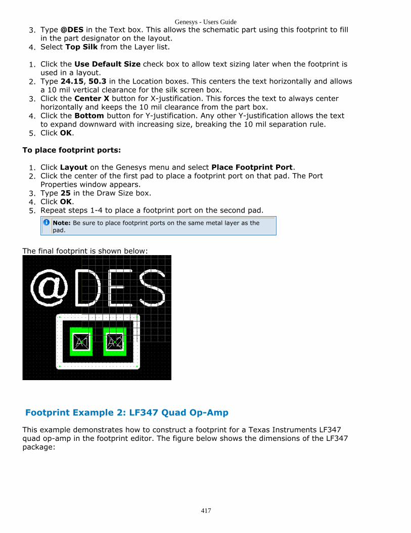
Genesys - Users Guide
417
Type @DES in the Text box. This allows the schematic part using this footprint to fill3.in the part designator on the layout.Select Top Silk from the Layer list.4.
Click the Use Default Size check box to allow text sizing later when the footprint is1.used in a layout.Type 24.15, 50.3 in the Location boxes. This centers the text horizontally and allows2.a 10 mil vertical clearance for the silk screen box.Click the Center X button for X-justification. This forces the text to always center3.horizontally and keeps the 10 mil clearance from the part box.Click the Bottom button for Y-justification. Any other Y-justification allows the text4.to expand downward with increasing size, breaking the 10 mil separation rule.Click OK.5.
To place footprint ports:
Click Layout on the Genesys menu and select Place Footprint Port. 1.Click the center of the first pad to place a footprint port on that pad. The Port2.Properties window appears.Type 25 in the Draw Size box.3.Click OK.4.Repeat steps 1-4 to place a footprint port on the second pad.5.
Note: Be sure to place footprint ports on the same metal layer as thepad.
The final footprint is shown below:
Footprint Example 2: LF347 Quad Op-Amp
This example demonstrates how to construct a footprint for a Texas Instruments LF347quad op-amp in the footprint editor. The figure below shows the dimensions of the LF347package:

Genesys - Users Guide
418
For this example, you set the current units to mils and place the pads first. Because this isa leaded part, use through holes at each pad location. The pins are 100 mils apart, so setthe pad center spacing at 100 mils. The hole diameter must be at least 21 mils toaccommodate the pins, but not exceed 33 mils, which is the width of the seating flange.For this example, the pad width is 75 mils, and the through-hole diameter is 30 mils.The figure below shows a pin-out diagram for the LF347 package:
You can create the above example as follows:
Place a viahole and pad1.Place ports for the first op-amp2.Place the positive power supply port3.Place ports for the second op-amp4.Place ports for the third op-amp5.Place the negative power supply port6.Place ports for the fourth op-amp7.Draw a silk screen box inside the pad perimeter8.Place the designator text9.Label the type of package10.
Please note the following:
Three ports are used for each of the op-amps shown in the pin-out diagram. Each op-amp is considered a part, so the footprint has four parts with three ports each.The port numbers are assigned according to the order that the associated schematic

Genesys - Users Guide
419
part uses. The order is found in the schematic part's diagram in the Referencemanual.In the OPA model, the non-inverting input is pin 1, the inverting input is pin 2, andthe output is pin 3.
Warning: Please adhere to this port numbering convention when creating a footprint. Otherwise,the rubber-band lines created by the layout indicate erroneous connections to make.
To place a viahole and pad:
Create a design with a layout.1.
Click the Viahole button ( ) on the Layout toolbar.2.Click in the Layout window to open the Viahole Properties window.3.Type 30 in the Drill Diameter box.4.Type 0,0 in the Location boxes because this is the first pad.5.Click the Square/Rect button for the pad shape. This identifies pin 1 during6.assembly.Type 75 in both the Pad Width and Pad Height boxes.7.Click OK.8.Repeat steps 2-7 to place a viahole with a round pad at location 100, 0, which9.properly spaces the hole centers. Specify 75 mils for the drill diameter and 30 milsfor the pad width and height.Place the remaining five pads for the first side at 100 mil increments as in step 8,10.with the final pad for the first side (labeled pin 7 above) set at 600, 0.Place the remaining viaholes at the same X-offset as the first side, with a Y-offset of11.310 mils (the distance given in the first figure above for the pin-to-pin crossdimension). The drill diameter and pad dimensions are the same as before.
To place the ports for the first op-amp:
Click the Port button ( ) on the Layout toolbar.1.Click in the Footprint editor to open the EM Port Properties window.2.Type 25 in the Draw Size box. This specifies a drawing size of 25 mils for the ports,3.which is large enough to see against a 75-mil pad.Assign this port to the first op-amp by choosing "A" in the "Device:" combo.4.Type 3 in the Port Number box. This assigns the op-amp output to pin 1 on the5.physical package.Select Top Metal from the Layer list. This places the layout objects on the metal6.layer before connecting to the pad.Type 0, 0 in the Location boxes. This centers the port on the first pad.7.Click OK.8.Repeat steps 1-8 to place ports 2 and 1 for device A on top of pads 2 and 3 at9.locations 100 , 0 and 200, 0.
To place the positive power supply port:
Click the Port button ( ) on the Layout toolbar.1.Click in the Footprint editor to open the EM Port Properties window.2.Type 300, 0 in the Location boxes.3.Since this port is not assigned to a schematic object, choose "None" in the Device:4.comboType 1 in the Port Number box.5.
To place ports for the second op-amp:

Genesys - Users Guide
420
Click the Port button ( ) on the Layout toolbar.1.Click in the Footprint editor to open the EM Port Properties window.2.Type 400, 0 in the Location boxes.3.The device should be set to "B", since this is the second op-amp in the package.4.Type 1 in the Port Number box. This corresponds to the non-inverting input.5.Repeat steps 1-5 to place two more ports for device B at locations 500, 0 and 600, 06.. Number the ports 2 and 3, corresponding to the inverting input and the output.The footprint should look like this:
To place ports for the third op-amp:
Click the Port button ( ) on the Layout toolbar.1.Click in the Footprint editor to open the EM Port Properties window.2.Type 600, 310 in the Location boxes.3.The device should be set to "C", and the pin number set to "3".4.Type 3 in the Port Number box.5.Repeat steps 1-5 to place two more ports for device C at locations 500, 310 and6.400, 310. Number the ports 2 and 1, corresponding to the inverting input and theoutput.
To place the negative power supply port:
Click the Port button ( ) on the Layout toolbar.1.Click in the Footprint editor to open the EM Port Properties window.2.Type 300, 310 in the Location boxes.3.The device should be set to "None".4.Type 2 in the Port Number box.5.Click OK.6.
To place ports for the fourth op-amp:
Click the Port button ( ) on the Layout toolbar.1.Click in the Footprint editor to open the EM Port Properties window.2.Type 200, 310 in the Location boxes.

Genesys - Users Guide
421
3.The device should be set to "D"4.Type 1 in the Port Number box.5.Repeat steps 1-5 to place two more ports for device D at locations 100, 310 and 0,6.310. Number the ports 2 and 3. corresponding to the inverting input and the output.
To draw silk screen box inside the pad perimeter:
Click the Line button ( ) on the Layout toolbar.1.Click in the Footprint editor to open the Line Properties window.2.Select Top Silk from the Layer list to place the line on the top silk layer.3.Type 10 (mils) in the Line Width box.4.
Note: To prevent silk screen interference with metal layer objects, all silk is kept at least 10 milsfrom the nearest metal.
Type -32.5, 257.5 in the Start boxes.5.Type 632.5, 52.5 in the End boxes.6.Click OK.7.Press the O key to create a 90-degree line.8.
Note: All of the above steps clear the pads by 10 mils, and extends to the edge of the pads on theopen ends of the footprint.
Draw another 10 mil line on Top Silk from -32.5, 257.5 to 632.5, 52.5. Press the O9.key to create a 90-degree line and then press the F key to flip the angle.
To place the designator text:
Click the Text Button ( ) on the Layout toolbar.1.Click in the Footprint editor to open the Text Properties window.2.Select Top Silk from the Layer list.3.Type @DES in the Text box.4.Click the Use Default Size check box.5.Type 300, 357.5 in the Location boxes.6.Click the Center X button for X-justification.7.Click the Bottom button for Y-justification.8.Click OK.9.
To label the type of package:
Click the Text Button ( ) on the Layout toolbar.1.Click in the Footprint editor to open the Text Properties window.2.Type LF347 in the Text box.3.Type 65 in the Size box. This text does not change with the default settings, and it is4.always the width of the silk screen box.Type 90 in the Angle box. This rotates the text counter-clockwise 90 degrees.5.Select Top Silk from the Layer list.6.Type 300, 357.5 in the Location boxes.7.Set the location to "-47.5,155".8.Click the Center X button for X-justification.9.Click the Bottom button for Y-justification. This places the text at the left edge of the10.silk screen box with a clearance of 10 mils.Click OK.11.
The footprint is now complete. The figure below shows the final footprint:

Genesys - Users Guide
422
Note: Be sure to place footprint ports on the same metal layer as thepad.
Using Pads in LayoutsA pad is a flat surface used to make electrical contact. There are three types of padsavailable: round, square, and wagon wheel. These three pad types are shown in the figurebelow:
Note: The wagon wheel is often used for thermal relief when connecting to a ground plane, which makessoldering easier.
Placing Pads in Layouts
You should place a pad in a layout wherever solder connections are made.To place a pad in a layout:
Click the Pad button ( ) on the Layout toolbar.1.Click in the layout where you want to place the pad. The Pad Properties window2.appears.Make the changes you want.3.Click OK.4.
Marking Pads as Grounded Objects
When pouring a ground plane polygon, the keep away applies to pads as well as to otherobjects. If a pad is marked as User Ground, the ground plane touches the pad (and anylines and arcs connected to it) instead of avoiding it.To mark a pad as a grounded object:
Double-click the pad to open its properties window.1.Click the User Ground check box.2.Click OK.3.

Genesys - Users Guide
423
Disabling Mask Generation for a Pad
The solder mask layer for a pad is automatically generated. If the pad's layer is marked asmirrored in the Layer table, the mask goes on the next mask layer below the pad's layer.Otherwise, the mask goes on the next mask layer above the pad's layer. If a mask is notneeded for a particular pad, you can turn it off for that pad.To disable mask generation for a pad:
Double-click the pad to open its properties window.1.Click the Don't Create Mask check box.2.Click OK.3.
Using Viaholes in Layouts
Viaholes are drilled, plated, through holes used to connect traces on different layers.Some viaholes are blind or buried, meaning they are not drilled through all layers.Viaholes automatically place a pad (round, square, or wagon wheel) on each metal layerbetween the start (top) and end (bottom) of the viahole, including pads on the start andend layers. The drill hole is always in the center of the pad. Electrically, viaholes connectevery layer between the start and end layers.Viaholes automatically generate solder mask for the two top and bottom pads. The shapeof the mask that is placed is identical to shapes placed for pads and is shown in the figurebelow.
If a mask is not needed for a particular viahole, you can turn it off.
Placing Viaholes in Layouts
Most viaholes are drilled through all layers. Blind or buried viaholes are not drilled throughthe entire board. These viaholes are useful in multilayer boards to connect some layerswhile leaving other layers unaffected. However, the production of boards with blind andburied viaholes is often more expensive.To place a viahole in a layout:
Select the Viahole button ( ) on the Layout toolbar.1.Click in the layout where you want to place the viahole. The Viahole Properties2.window appears.Make the changes you want.3.Click OK.4.
To place a blind or buried viahole in a layout:
Select the Viahole button ( ) on the Layout toolbar.1.Click in the layout to place the viahole. The Viahole Properties window appears.2.Clear the Use Default Layers check box if it is selected. This lets you change the3.start and end layers.Select the start and end layers from the Start and End Layer lists.4.Make any other changes you want.5.Click OK.6.
Marking Viaholes as Grounded Objects

Genesys - Users Guide
424
When pouring a ground plane polygon, the keep away applies to viahole pads as well as toother objects. If a viahole is marked as User Ground, then the ground plane touches theviahole pads (and any lines and arcs connected to them) instead of avoiding them.To mark a viahole as a grounded object:
Double-click the viahole to open its properties window.1.Click the User Ground check box.2.Click OK.3.
Disabling Mask Generation for a Viahole
The solder mask layer for a viahole is automatically generated. If the viahole's layer ismarked as mirrored in the Layer table, the mask goes on the next mask layer below theviahole's layer. Otherwise, the mask goes on the next mask layer above the viahole'slayer. If a mask is not needed for a particular viahole, you can turn it off for that viahole.To disable mask generation for a particular viahole:
Double-click the viahole to open its properties window.1.Click the Don't Create Mask check box.2.Click OK.3.
Adding Polygons, Pours, and Ground PlanesPolygons are filled areas on the layout. You can use polygons on any layer, create one ofany shape, and even have ones with cutouts (holes). A pour is a polygon that is pouredaround other objects on the same layer. Pouring a polygon causes it to keep away fromother objects by a specified distance. Pours are especially useful for constructing groundplanes, which can touch objects marked as User Ground while keeping away from otherobjects.
Constructing Polygons
Polygons are often used for landing pads with unusual shapes. Use polygons only whennecessary if you plan to create a Gerber file from the layout, because polygons candrastically increase the disk size of a Gerber file. Some typical polygons are shown below:
To construct a polygon:
Click the Polygon button ( ) on the Layout toolbar.1.Click the first vertex (corner) of the polygon.2.Click the next vertex.3.
Note: If the last point placed is incorrect, press the Backspace key to remove it.
Continue clicking all vertices.4.Double-click the last vertex (or click the first vertex again) to complete construction5.of the polygon.
To add a cutout (hole) to a polygon:
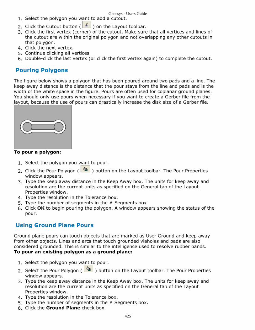
Genesys - Users Guide
425
Select the polygon you want to add a cutout.1.
Click the Cutout button ( ) on the Layout toolbar.2.Click the first vertex (corner) of the cutout. Make sure that all vertices and lines of3.the cutout are within the original polygon and not overlapping any other cutouts inthat polygon.Click the next vertex.4.Continue clicking all vertices.5.Double-click the last vertex (or click the first vertex again) to complete the cutout.6.
Pouring Polygons
The figure below shows a polygon that has been poured around two pads and a line. Thekeep away distance is the distance that the pour stays from the line and pads and is thewidth of the white space in the figure. Pours are often used for coplanar ground planes.You should only use pours when necessary if you want to create a Gerber file from thelayout, because the use of pours can drastically increase the disk size of a Gerber file.
To pour a polygon:
Select the polygon you want to pour.1.
Click the Pour Polygon ( ) button on the Layout toolbar. The Pour Properties2.window appears.Type the keep away distance in the Keep Away box. The units for keep away and3.resolution are the current units as specified on the General tab of the LayoutProperties window.Type the resolution in the Tolerance box.4.Type the number of segments in the # Segments box.5.Click OK to begin pouring the polygon. A window appears showing the status of the6.pour.
Using Ground Plane Pours
Ground plane pours can touch objects that are marked as User Ground and keep awayfrom other objects. Lines and arcs that touch grounded viaholes and pads are alsoconsidered grounded. This is similar to the intelligence used to resolve rubber bands.To pour an existing polygon as a ground plane:
Select the polygon you want to pour.1.
Select the Pour Polygon ( ) button on the Layout toolbar. The Pour Properties2.window appears.Type the keep away distance in the Keep Away box. The units for keep away and3.resolution are the current units as specified on the General tab of the LayoutProperties window.Type the resolution in the Tolerance box.4.Type the number of segments in the # Segments box.5.Click the Ground Plane check box.6.

Genesys - Users Guide
426
Click OK to begin pouring the polygon. A box appears showing the status of the pour.7.
Importing and Exporting Layout FilesGenesys lets you import or export layouts using many file types. Importing a layout letsyou use layouts created in other programs. Exporting a layout using one of the supportedfile types lets you use a Genesys layout in other programs and ensures it is understood bya boarding manufacturer.
Importing Layout Files
You can import a layout using any of the following file types:
6.x Model LibraryDXF FileExcellon (Gerber) Drill ListGDSII FileGerber FileXML File
To import a layout file:
Click File on the Genesys menu and select a file type from the Import menu.1.Follow the instructions in the windows that appear.2.
Exporting Layout Files
You can export a layout using any of the following file types:
ASCII Drill ListBill of MaterialsDXF FileExcellon (Gerber) Drill ListGDSII FileGerber FileHPGL FilePart Placement ListXML File
To export a layout file:
Open (or select) the layout window to make the Layout the active window.1.Click File on the Genesys menu and select a file type from the Export menu.2.Follow the instructions in the windows that appear.3.
Using Gerber FilesA Gerber file lets you export layouts using a commonly used format. This lets you uselayouts in other programs or export them to board manufactures in a standard formatthey understand. A circuit board can have many layers; therefore, a Gerber file is createdfor each layer.
Importing Gerber Files
You can import Gerber files for use in generating or modifying layouts.To import a Gerber file:

Genesys - Users Guide
427
Click File on the Genesysmenu and select Gerber File from the Import menu.1.Click the file you want to import.2.Click Open.3.Specify options for importing the file.4.Click OK.5.
Exporting Gerber Files
You can write a Gerber file for the current layout.To export a Gerber file:
Click File on the Genesysmenu and select Gerber File from the Export menu.1.Specify options for exporting the file.2.Click OK.3.Click the name of the file.4.Click Save.5.
Using Custom Apertures
Custom apertures are apertures created by a layout specifically for each Gerber file. TheAperture list contains a list of user apertures defined by users for specific needs.Generally, you should use user apertures only if your company has a standard set ofapertures to which Gerber exports must conform. Otherwise, you should use customapertures.A layout has a built-in optimization routine that selects the best list of apertures forefficient polygon fills and flashes. These custom apertures result in the smallest possibleGerber files, whereas a user list can give very inefficient, incorrect, and large files.
Editing the Aperture List
Use the Editing Aperture List window to customize apertures in a Gerber file.To edit an aperture list:
Click File on the Genesysmenu and select Gerber File from the Import menu.1.Click the Options tab.2.Clear the Generate Custom Apertures check box.3.Click the Edit DEFAULT.APL button.4.Make the changes you want.5.Click OK.6.

Genesys - Users Guide
428
LiveReportsA LiveReport is a living page that can contain live views of various kinds of Genesysobjects. You can mix Graphs, Designs, Equations, Notes, Tables, and Datasets all in asingle printable and viewable page. Below is an example of a LiveReport page from thesimple Bridge-T Example.
It's a Live Report because you can click in any of the windows on the page and workexactly as you would work in single windows in Genesys. The border turns green when awindow is active, as seen below.

Genesys - Users Guide
429
When you want to move or resize a window within a LiveReport click the black border(box) outside the window and it will turn yellow and gain handles you can drag/move.

Genesys - Users Guide
430
To use the LiveReport rather than one of the windows, click outside all of the windows andyou will see the LiveReport toolbar and the LiveReport menu. No windows will be green oryellow.
ContentsCreating a LiveReport (users)Supported LiveReport Object Types (users)View Window in LiveReport (users)Arranging Views (users)LiveReport Properties (users)
Creating a LiveReportTo manually create a LiveReport:
Click the New Item button ( ) on the Workspace Tree toolbar, select *add*1.LiveReport....If desired, change the LiveReport name, layout, or other properties. 2.Click OK to create the LiveReport or click Cancel to not create the new LiveReport.3.
Supported LiveReport Object TypesLiveReports supports most of the standard Genesys object types.
Object Type Supported? Limitations
Graph yes A Graph has a single aspect ratio. If you have an open graph and a graph inreport only the only the graph that is currently selected will own the aspectratio.
Design yes (partial) Not supported - Parameters, PartList, and SubstrateSet
Notes yes
Datasets yes
Equations yes
Scripts yes
Tables yes
Analyses no Linear, Transient, ... have no view
Evaluations(sweeps)
no Evaluations have no view
Syntheses no Syntheses have no view
Substrates no Substrates have no view
Adding a View Window to a LiveReportThere are two ways to put objects (windows) on a LiveReport.
Right-click the page and select Insert then select one of the objects listed to insert awindow with that object.

Genesys - Users Guide
431
Drag-drop an object from the workspace tree into the page using the mouse leftbutton.
......................
Removing a Window from a LiveReportSelect the surrounding rectangle (click it or select multiple with the select tool and draw abox) and then either click the Del key or right-click the mouse and select Delete... fromthe menu.

Genesys - Users Guide
432
Arranging ViewsUse the LiveReport Arrange Views dialog box to arrange the sub-objects of a LiveReport.
Automatic - In general, automatic arrangement is quick, easy, and does a reasonable jobof laying out the view windows.
If a window is not placed in the desired location when OK is clicked, simply drag thewindow into place and swap it with another, then re-do the Arrange Views.
If the LiveReport page is not divided in the desired fashion, use one of the Best Fit or Splitoptions.

Genesys - Users Guide
433
Best Fit - The best-fit options arrange sub-objects in a tiled arrangement, similar to theway Windows arranges Tiled views. The images show the order of the major and minorpage splits.
Split Horizontally / Vertically - Arrange sub-objects so they are ordered in a linearfashion and are all the same size.
Inter-object Spacing - The distance (gap) between the arranged views. The units canbe set in Page Properties.
Sort Alphabetically - This rarely-used option sorts the views by name, instead of theusual geometric positioning based on current pane positions. This options is mostly usedto display libraries of symbols or parts.
The images to the left of the radio buttons may be double-clicked to quickly select an arrangement andclose the dialog box.
LiveReport PropertiesThere are several tab pages that you can use to change the properties of a LiveReport:
Page PropertiesMargin PropertiesHeader and Footer Properties
To change the properties of a LiveReport:
Double-click the report or click LiveReport on the Genesys menu and select1.Properties.Click the desired tab.2.Make the changes you want.3.Click OK.4.
When double-clicking the LiveReport, Genesys uses the mouse cursor location to pick an appropriatetab. Double-click the upper or lower page area to initially display the Header & Footer page;double-click the side margins to initially display the Margins page; anywhere else displays the Pagesettings tab page.
Page Properties
Use the LiveReport Page Properties tab page to change the general properties of aLiveReport.

Genesys - Users Guide
434
Name - The name of the LiveReport.1.Description - The LiveReport description (optional).2.Use long names on titles - When checked, the sub-object view windows will show3.the full workspace pathname in their title.Paper Size - Use this combo-box to set your page size.4.Orientation - Sets the page to portrait (tall) or landscape (wide) mode.5.Width & Height - The size of the paper (in current units).6.Grid Spacing - The distance between grid dots.7.Units - The units used by LiveReport for all of its settings, including margins and8.arrangement spacing.Font - The page font, which is used for sub-object titles.9.
Margin Properties
Use the LiveReport Margins Properties page to change the margins of a LiveReport.
Top, Left, Right, Bottom - The margin widths to use for the page. The margins are1.shown by a light-gray, non-printing box; the box can be hidden using the eye toolbarbutton menu.Units - The units used by LiveReport for all of its settings can be set on the Page tab.2.

Genesys - Users Guide
435
Header and Footer Properties
Use the LiveReport Header & Footer Properties page to change the margins of aLiveReport.
Header - When checked, the header is enabled. It will print at the top of the1.LiveReport page. The text is completely customizable; strings such as "CompanyConfidential" may be used. Also, macro strings like "%DATE%" and "%TIME%" willbe converted into the actual date, time, filename, etc.Font - Sets the header font.2.Justification - Determines the header horizontal justification (left / centered / right3.).Footer - The footer works just like the header, but is printed at the bottom of the4.page.

Genesys - Users Guide
436
Managing LibrariesLibraries serve as a container for parts, designs, equations, and lots of other Genesysobjects. They let you keep all of your objects in one place, which makes it easier for youto organize the contents. Genesys provides a number of libraries for your convenience andallows you to add custom libraries. Libraries that are added will be auto-loaded whenGenesys starts.
There are two dialog boxes in Genesys that allow you to interact with Libraries: TheLibrary Selector and the Part Selector. There is also a Library Manager dialog box thatallows you to do things such as import and remove libraries.
The two dialog boxes that enable the interaction with objects are the Library Selector andthe Part Selector.
The Library Selector allows interaction with all object types except parts, since the PartSelector is used to interact with Parts. You can think of the Part Selector as a specializedLibrary Selector where the Library object type is Parts. Both the Library Selector and PartSelector allow you to bring objects into your workspace or view objects that you have putinto them from the workspace. A search text box is provided in both selectors to help youfind objects in your libraries.
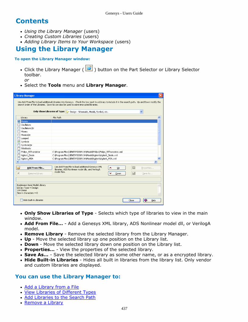
Genesys - Users Guide
437
ContentsUsing the Library Manager (users)Creating Custom Libraries (users)Adding Library Items to Your Workspace (users)
Using the Library Manager To open the Library Manager window:
Click the Library Manager ( ) button on the Part Selector or Library Selectortoolbar.orSelect the Tools menu and Library Manager.
Only Show Libraries of Type - Selects which type of libraries to view in the mainwindow.Add From File... - Add a Genesys XML library, ADS Nonlinear model dll, or VerilogAmodel.Remove Library - Remove the selected library from the Library Manager.Up - Move the selected library up one position on the Library list.Down - Move the selected library down one position on the Library list.Properties... - View the properties of the selected library.Save As... - Save the selected library as some other name, or as a encrypted library.Hide Built-in Libraries - Hides all built in libraries from the library list. Only vendorand custom libraries are displayed.
You can use the Library Manager to:
Add a Library from a FileView Libraries of Different TypesAdd Libraries to the Search PathRemove a Library

Genesys - Users Guide
438
Edit the Properties of a LibraryExport an Encrypted Library
Add a Library from a File
Select the Add From File... button to add a Genesys XML library, a ADS Nonlinear Modeldll, or a VerilogA model to the Library Manager. Genesys ships with a huge range ofprebuilt vendor libraries (parts and models) located in the Model folder of the Genesysdirectory. The Model folder also contains all of the VerilogA and ADS Nonlinear modelsthat ship with Genesys.
Adding XML Libraries
Click the Add From File... button.1.Browse to the folder with the XML library you want to use.2.Select one or more libraries (use Shift+Click, Ctrl+Click, or Ctrl+A to select more3.than one).Click Open to add the library or Libraries to the available Libraries.4.
Adding XML Libraries via Drag-Drop
Find the XML libraries you want to add using Windows Explorer. Select all of thelibraries and drag then drop them into the Genesys work area.
In the image above we add 5 new libraries (one part library and four model libraries) toGenesys.
Adding VerilogA Models
In the Library Manager, select the Add From File... button.1.Set the Files of Type field to VerilogA Model Files (*.va, *.cml).2.Browse for and select the VerilogA model you wish to add.3.Click Open.4.

Genesys - Users Guide
439
The VerilogA file is added to the Library Manager as a Library as shown below.
Note: Each added VerilogA .va/.cml file will automatically create a matching xml library for use withinGenesys.
Adding ADS Nonlinear Models

Genesys - Users Guide
440
In the Library Manager, select the Add From File... button.1.Set the Files of Type field to ADS Nonlinear Model DLL Libraries (*.dll).2.Browse for the and select the ADS Nonlinear model you wish to add.3.Click Open.4.Choose to save the model into and existing library or to create a new library.5.Click OK6.
The DLL file must be in the MINT format. Only MINT model DLLs can be added this way.
The model is added to the library of your choice. Multiple models can be added to thesame library.

Genesys - Users Guide
441
View Libraries of Different Types
The Library Manager lists all of the libraries that are currently loaded into Genesys. Usethe dropbox Only Show Libraries of Type to select which type of libraries to view in theLibrary Manager.
The selection Design - Schematic, Model, Symbol, etc. shows all libraries that containschematics, models, or symbols. Notice that if you change the Type to Equation onlylibraries of equations are shown in the Library Manager.
Adding Libraries to the Search Path
The checkbox next to each library determines whether or not the library is included in thesearch path. Once a library has been added to the search path, it will always be in thesearch path unless you manually remove it. Libraries at the top of the list have the highestpriority in the search path. Use the Up and Down buttons to move libraries around in thelist.

Genesys - Users Guide
442
This feature is useful for libraries of custom models or symbols that you may have. Modelsand symbols from libraries that are included in the search path can be type in the ChangeModel or Change Symbol dialogs. For example, a library called MyModels that contains amodel called CustomFilter has been added to the Library Manager and added to the searchpath. The model CustomFilter or any other model in MyModels can now be entered in theChange Model dialog directly.
Adding the MyModels library to the search path removes the need to type CustomFilter@MyModels or toadd the model from the library to the workspace tree in order to use the model in a part.
Another helpful tip is to add custom Equation libraries to the search path. Functions in anEquation library that has been added to the search path can be called directly from anyequation block. For example, a library called "MyEquations" that contains a function calledMyFunction is added to the Library Manager and included into the search path. Thefunction MyFunction or any other function in MyEquations can now be called from anyequation block.
Functions in the MyEquations library do not need to be added to the workspace if MyEquations has beenadded to the search path.
Removing a Library
When you remove a library, you only remove it from the Library box in the LibraryManager. The external library file is not deleted.
You cannot remove the Internal libraries. These libraries are read-only.
To remove a library from the Libraries list:

Genesys - Users Guide
443
Click the name of the library in the Library Manager dialog.1.Click Remove Library.2.
This does not delete the library file. It just assures that the library is not auto-loaded the next time yourun Genesys.
Editing Library Properties
You can use the Library Manager to edit the properties of your libraries such as the nameor description of the library.
To edit the properties of a library:
Click the name of a library in the Library list.1.Click the Properties... button.2.Make the changes you want, and then click OK.3.
You cannot edit Internal libraries nor can you edit Encrypted Libraries. These libraries are read-only.
Export an Encrypted Library
Genesys supports encrypting and using encrypted libraries. The option to encrypt a libraryis accessible through the Library Manager, which itself is accessible from the LibrarySelector (View/Docking Windows/Library Selector) or the the Tools Menu. Once you havecreated a custom library, you may save it as encrypted.
In the Library Manager, select your custom library and click the Save As... button on theright.
In the Save As dialog box, there is a checkbox labeled Save Encrypted on the lowerright. Check this box as shown here:

Genesys - Users Guide
444
The library will then be saved as encrypted. If the library you are encrypting is a DesignLibrary, you will not be able to view the contents of the designs' part lists or equations.
Creating Custom LibrariesA custom library can contain custom parts or designs (models and symbols and circuits),or anything else. Each Library Manager section can only hold custom libraries of itsspecific type (so you can not use a design library in the part selector, you can not use aDataset library in the design selector, and so on).
To create a custom library
Right click an object in the workspace tree or for a part right click a part in the Part1.SelectorSelect New Library... from the Copy To menu2.

Genesys - Users Guide
445
Set the library name.3.If you want, browse for a different path for the new library. We recommend the My4.Workspaces folder for libraries, though.Click OK.5.
Adding Library Items to Your WorkspaceAny object in a library can be added to your workspace. In the case of Symbols or Modelsyou can just double-click (or edit) the object in the Library Selector. You can use thelibrary selector to add any object type into your workspace.
If you don't want the docking library selector to be visible (taking up screen real estate)use the Add From Library Option as seen below.
Parts are special. They are not added (separately) to your workspace, but instead, are placed using amouse onto a schematic design.

Genesys - Users Guide
446
To Insert an Object from a Library into your workspace
Select From Library...1.Set the Library Type to the type of object you want to insert in your workspace2.Set the Current Library to the Library you want to add from3.Double-click the specific Object you want to add.4.

Genesys - Users Guide
447
OptimizationPractical design problems such as standard values, component tolerances, and parasiticsmay preclude a purely theoretical solution. When only a few variables in a schematicrequire adjustment, manual tuning is effective. As the number of variables increases,visualization of the multidimensional variable space is difficult, and tuning becomes lesseffective. Optimization is used to solve these types of problems. Optimization is often acompromise of conflicting requirements with no exact solution. Effective use ofoptimization consists of tuning variables according to some algorithm, running asimulation, comparing the results to specified goals, and repeating the process until anacceptable error level is achieved.
ContentsUsing Optimization (users)Creating an Optimization (users)Cost Function (users)Optimization Methods (users)
Creating an OptimizationTo create an Optimization:
Click the New Item button ( ) on the Workspace Tree toolbar and select AddOptimization from the Evaluations submenu.
Select Analyses to Run
The General tab page sets which analyses will run when you optimize, whatoptimization method to use, the name of the optimization, etc.

Genesys - Users Guide
448
Name – The name of the optimization, which will be shown in the workspace tree.Description – A description of this optimizaion, to help you keep track of multipleoptimization and to hold notes specific to this item.Optimization Method – Which optimization technique to use
Automatic – Cycles between gradient and pattern searches until no furtherimprovement is possible. This is the recommended setting.Gradient Search – Locate a local minimum of the error terms.Pattern Search – Locates a global minimum.
Cost Function – Selects which cost function to useLeast Squares (L2 Norm) – A method used to find an approximate solutionwhich minimizes the sum of the squares of the error terms. This is a second-order function.Smoothed Worst Case (L6 Norm) – A sixth-order approximation, whichmaximizes the minimum value of the current position. This is the same costfunction as the old, mis-named MiniMax option in earlier versions of Genesys.Worst Case (L∞ Norm) – An infinite order approximation, which maximizesthe minimum value of the current position.
Calculate Now – Closes the property window and runs the optimization with thecurrent settings.Factory Defaults – Resets the optimization settings to the original default settings(when you first installed Genesys).Analysis List – Determines which analyses will run when you optimize; check themon or off to enable them.
Select Goals
Determine the goals of the optimization in the second tab.
Default Dataset or Equations – Indicates the default source of the measurements,unless the measurement itself specifies another dataset.Goal rows – Each grid row describes a goal for the optimizer, which is discussed in

Genesys - Users Guide
449
detail below.Add – Adds another row to the Goal table.Remove – Click a row to select it, then click Remove to get rid of it.Measurement Wizard – Brings up a window, to let you easily select a measurementto add to the Goal table.Current Error – Displays the error term, using the curent values of themeasurements.Stop if the Total Error is less than – Specifies a stopping point for theoptimization.
NoteCurrent Error is based on the current values of the measurements listed in the Goals table. If themeasurement (or its dataset) does not yet exist, "N/A" will be displayed, since the error term cannot beevaluated. Also, if any of the measurements already meet the specified goal, its contribution to CurrentError is zero (0), so changing its Weight will have NO EFFECT on the Current Error.
This optimization block is for a filter. It instructs Genesys to try to make the forward gain(S21) at least -.1 dB and the input reflection (S11) better than (less than) -15 and -25dB. The frequency range (because Sij is frequency dependent) for all targets is anequation dependent on fL (defined in workspace Equations), with a loose range for S21and two ranges for S11 (tighter for the -25dB constraint). Finally, the Weight of the S21target is 10, meaning that the optimizer will put more importance on that target than onthe two S11 targets.
Each row specifies an optimizer goal, using one or more of the Measurements describedin the Simulation manual, as well as any other valid equation.
If Use is checked, this goal will be used by the optimizer; if unchecked it will be ignored
Op – The available operators are =, >, < and %.
The = operator attempts to optimize to the specified target value. (note that theerror function will rarely reach zero when using the = operator)< or > attempt to optimize a parameter to be less than or greater than the specifiedtarget value.The % operator attempts to flatten the specified parameter, without regard tospecific value of the parameter. When using the % parameter, the target value isused to indicate acceptable peak-to-peak value of the given parameter. Forinstance; Target of db(S21) with operator % and target of 0.2 describes the desire toflatten S21 to within 0.2 dB. When the P-P value is less than the target, the termadds nothing to the error function. To specify a flattening command that flattens thedesired measurement completely, enter a target of 0.
This four line set of targets for a bandpass filter:
Measurement Op Target Weight Min Max
db(S21) < -40 1 10 40
db(S21) > -1 1 55 85
gd(S21) % 1 100 130
db(S21) < -40 1 100 130
attempts to achieve at least 40 dB of rejection in lower and upper stopbands and less than1 dB insertion loss with flat delay in the passband.
This four line optimization block for an amplifier

Genesys - Users Guide
450
Measurement Op Target Weight Min Max
db(S21) > 11.5 1 2000 4000
db(S21) < 12.5 1 2000 4000
db(S11) < -10 1 2000 4000
db(S22) < -10 1 2000 4000
attempts to achieve better than 10 dB of return loss in an amplifier with 11.5 to 12.5 dBof gain. A similar optimization block would be
Measurement Op Target Weight Min Max
db(S21) = 12 1 2000 4000
db(S11) < -10 1 2000 4000
db(S22) < -10 1 2000 4000
Tip: To reduce optimization time, specify a minimum number of frequency points.
Select Variables to Optimize
When the optimization runs, it will automatically tune the variables listed in the Variableswindow.
Enter a value in Min and/or Max to set limits on the variables. A blank entry impliesno limit.Check Long Variable Names to see the entire name of the variable (as shownabove).Click Add to add a new variable to the list. This brings up the Select Variables toTune dialog, as described below.Click a Min or Max column entry then click Remove to remove a variable from thelistClick Get Tuned Variables to get all currently tuned variables (the contents of theTune docking window)

Genesys - Users Guide
451
Click Copy Settings Down to copy Min and Max from the top row to the remainingrows.
If you do not specify any variables to use, the Optimizer will use the current set of Tunable variables asseen in the Tune Window.
Check the variables you want to add to the optimization set.
Caution: It is very important that the frequencies at which the circuit is optimized are also frequenciesincluded in the simulations. Optimization will not create any new simulation frequencies.
Select Optimization Method Options (advanced)

Genesys - Users Guide
452
Options for the optimizer:
Gradient
Gradient Method – selects the algorithm which the gradient optimizer will use.Automatic – Automatically cycles through the gradient algorithms (listedbelow) until no further improvement is possible. This is the recommendedsetting.Steepest Descent – This technique is a first-order optimization algorithm. Ituses steps proportioal to the negative of the gradient at the current location tofind the local minimum.Fletcher-Reeves – One of the three common conjugate gradient methodfunctions; it may converge faster than the steepest-descent algorithm.Polak-Ribière – This technique is an alternative to the Fletcher-Reeves formulawhich attempts to avoid the problem of progressively "lost conjugacy of thegenerated directions", due to inaccuracies of the linear searches and the non-quadratic terms of the Fletcher-Reeves method.Hestenes-Stiefel – A third conjugate gradient method function, which is similarto the Lanczos method to symmetric matrices, but which uses coupled two-termrecurrences, instead of the Lanczos three-term formulation.
Use Squared Error – determines how quickly the algorithm accelerates.Gradient multiplier – the distance the gradient search travels at each iteration.Line Searches (max) by default the gradient search up to 10 times (and at least 5)along a single gradient line to find the best fit. This could cause a slowdown with noimprovement in convergence.Delta – in percent, the amount the variables are perturbed to calculate a delta forthe gradient. 1e-3 is average. If the optimizer gets stuck and can't improve you maywant to decrease this. If the convergence is too slow you may want to increase this.Values above .1 or below 1e-8 are not recommended.Maximum pattern rounds – during automatic optimization the pattern search won'tdo more than this # of rounds before returning to gradient search.

Genesys - Users Guide
453
Pattern
Initial step size – Primarily for automatic optimization; this is the initial patternstep size. Note: This is now a percentage, but it used to be a fractional amount:50% is the same as the previous 0.5 setting value.Allow Grid Search – The grid search algorithm is designed for only 2 or 3parameters and then it generally isn't as good as a well tuned pattern search, but weallow it as an option for discontinuous searches. Enable this carefully as it may seemto hang the system with a lot of parameters.Allow Multivariate Optimization – If the problem does not converge you maywant to enable this. This will converge better with paired parts (e.g. LC circuits) butwill be slower on standard problems.Allow Pattern Rotation – This lets the pattern search be order independent.Allow Random Pattern Search – Enables random search during a Pattern searchiteration.
Random – These settings are enabled on the General tab page, via the "Allow InitialRandom Search" checkbox.
Perturbation of Tuned Variables – The percentage amount to vary the selectedtunable variables (on the Variables tab).Maximum Random Search Steps – Specifies how many search steps may be used.
Cost FunctionA cost function is created from goal values, goal weights, and actual values.
For Least Squares and Smoothed Worst Case the equation is:
For Worst Case Error the equation is:
where
n = Number of goalsp = Power of error function ( 2 for Least Squares, 6 for Smoothed Worst Case )Gn = Set of goal valuesVn = Set of actual valuesWn = Set of goal weights ( default weight = 1 )
Optimization routines attempts to minimize the cost error by changing user specifiedvariables during an optimization simulation.
Weights
Default weight values are set to 1. Weight values greater than one (such as 10) make the

Genesys - Users Guide
454
goal more important. Weight values between zero and one (such as 0.1) make the goalless important.
For many optimizations, weight values are unnecessary. This is often the case when thespecified goals are similar in value. Use of < and > operators instead of = also reducesthe need for weights. When the error resulting from a parameter is zero because thecondition has been satisfied, the weight multiplier has no effect.
When the optimized parameters represent a wide range of goals, weights are used toobtain a more desirable solution. Remember, optimization is a search for a compromise.Weights are not used to obtain a "correct" solution, but rather to "sculpt" a solution moredesirable to the user. The user observes the optimization results and then modifies theparameter goals and weights to obtain a "better" solution.

Genesys - Users Guide
455
Optimization MethodsThis section documents additional technical details for the optimization methods.
GradientThe following gradient methods can be used:
Steepest Descent1.Fletcher-Reeves2.Polak-Ribiere3.Hestenes-Stiefel4.
Steepest Descent
Algorithm for Steepest Descent
Start at a point X 01.
Calculate F(X 0)2.
Calculate the next X n according to: 3.Calculate the next F(X n)4.
Repeat steps 3 and 4 until the minimum value is achieved5.
Nonlinear Conjugate Gradient Methods
The following methods fall into the nonlinear conjugate gradient methods:
Fletcher-Reeves1.Polak-Ribiere2.Hestenes-Stiefel3.
For a quadratic function:
The minimum is obtained when the gradient is 0.
For linear conjugate gradients methods a solution is sought for the linear equation:
However, the gradient alone is used to find the local minimum for the nonlinear conjugategradient methods.
Algorithm for Initial Point
Start in the Steepest Descent direction: 1.Perform a line search in the steepest direction until the minimum value is reached:2.

Genesys - Users Guide
456
and
Algorithm for Remaining Points
Calculate the steepest direction: 1.Compute according to one of following nonlinear conjugate gradient methods2.Update the conjugate direction: 3.
Perform a linear search and optimize: 4.Update the new position: 5.
If the function is a pure quadratic the minimum will be reached in approximately Niterations. A non-quadratic will make slower progress.
Fletcher-Reeves
Polak-Ribiere
Hestenes-Stiefel
PatternAlgorithm for Pattern Search
Find the initial error (E initial) from all initial variable values1.
Find the variable that produces the lowest error (loop through each variable)2.Find error (E hi) from current variable multiplied by adaptive step1.
Find error (E lo) from current variable divided by adaptive step2.
Step size is reduced and repeats steps a and b for all variables to find the best3.error (E best)
Now the best error has been found for the variable repeat step 2 to see if we can find3.the next variable that has the best errorRepeat step 3 to keep minimizing the error for each variable that is the largest4.contributor to the error
RandomAlgorithm for Random Search
Find a random value 1 for every variable1.

Genesys - Users Guide
457
Calculate the cost error function2.If the stop error value has been achieved then stop3.If we have not met the stop error value then repeat steps 1 through 3 until the4.maximum number of steps is reached
1 A uniform distribution is used. If a value has hard limits those are used. However, ifthere are no limits then the specified percentages are used for both lower and upperlimits.

Genesys - Users Guide
458
Using OptimizationA variety of search methods can be used to minimize the error of a selected cost function.Cost functions relate goals and actual values to create an error number. The value of thiscost error is mostly meaningless. However, it's magnitude indicates whether the solutionis getting closer or farther away from the specified goals. Variables controlled by theoptimization can be selected and limits can be placed on these variables by the user. Theoptimizer will change these variables according to the selected optimization method thenwill run a simulation and compare a current error with lowest achieved error to determineif the variable changes are going in the right direction. These variable changes willcontinue to occur until the cost error reaches zero or doesn't improve after variousattempts.
The Optimization Methods are:
Automatic (default)1.Gradient2.Pattern3.
The cost functions are:
Least Squares (L2 Norm) (default)1.Smoothed Worst Case (L6 Norm)2.Worst Case Error (L inf Norm)3.
Optimization MethodsIf enabled, a Random search is used initially to randomly find the best starting point.
NoteFor more details on these methods see Optimization Methods (users).
Automatic
If the Random search has been enabled then this method will be invoked first to try andfind the best overall global minimum. The Simplex method is used in conjunction with therandom search to find the best global local minimum. Once the maximum number ofglobal search attempts has been exceeded a pattern search is selected to find a localminimum. The pattern search is used in conjunction with the gradient method to find alocal minimum. If the cost error is hasn't met the stop error criteria and yet there is noimprovement in the error over a number of iterations the entire process will be repeatedto ascertain whether a better minimum occurs elsewhere. This process will continue untilthe cost error reaches zero or the user specified stop error is reached.
Visually, that looks like:

Genesys - Users Guide
459
Gradient
There are several gradient methods:
Automatic (default)Steepest DescentFletcher-ReevesPolak-RibiereHestenes-Stiefel
See Optimization Methods (users) for details about these methods.
When Automatic is selected the optimizer will try each gradient method to determine thebest error. It will continue to use that method until the error doesn't improve. If the errordoesn't improve another method will be selected.
Gradient methods are very effective in the early phase of an optimization. It is reasonablytolerant of poor initial component values and a large number of components. It oftenmakes significant progress after only a few rounds. However, gradient search algorithmprogress tends to halt before achieving optimum final values since this method tends toonly find local minimums.
Pattern

Genesys - Users Guide
460
In this algorithm, each element is stepped up and down and the errors are recorded. Onlythe element with the best error reduction is permanently changed. This process repeats byagain searching for the element with the best error reduction. This algorithm thereforeattempts to align with search in an optimum direction.
The Pattern search is based on an optimizer described in the paper, "The Effectiveness ofFour Direct Search Optimization Algorithms", Randall W. Rhea, IEEE 1987 MTT-SInternational Microwave Symposium Digest, June 9, 1987. The implementation uses anadaptive and independent variable step size to increase the resistance to "hang."
Random
The method is used when a good starting point is not known. All variables are perturbedwithin a user specified percentage for a given number of steps. When a better error isachieved this becomes the starting point for the next randomization of variables. Theminimum error found for the specified number of steps will be used as a starting point forthe rest of the optimization.
This method if a fairly costly method since it doesn't rely on information from one step tothe next to predict where the minimum is.
NoteThe random search mode is only available when enabled on the 'General' tab.
Cost FunctionsSee Cost Function (users) for additional details.
Least Squares (L2 Norm)
This cost function is generally used when all goals are equally as important.
Smoothed Worst Case (L6 Norm)
This cost function is generally used when emphasizing the goal with the worst error.However, other goals are still considered with much less emphasis. This function doesn'thave discontinuities.
NoteThe Smoothed Worst Case is the same algorithm called Minimax in versions prior to Genesys 2010.05.
Worst Case Error (L inf Norm)
This cost function is used when only the worst case goal matters. All other goals areignored unless they become the worst case goal as the worst case goal errors are beingreduced.
Optimization OutputDuring a simulation the optimizer status is written to the status window, showing thefollowing information:

Genesys - Users Guide
461
Field Description
Round Integer value that indicates the total number of times a new direction if found to a lower cost orerror value. One round involves 1 or more steps.
Step Integer value that indicates the total number of calculation steps performed.
SearchType
Shows the optimization method used. For a Gradient Search the Gradient Method will also beshown along with the number of successful rounds yielding a lower cost or error value.
Best Error Best error achieved over the total number of steps.
CurrentError
Error for the current step.

Genesys - Users Guide
462
Parts, Models and Symbols Contents
Parts (users)Models (users)Symbols (users)Mapping Symbols to Models in Parts (users)Finding Symbols and Models during Simulation (users)Symbol Reference (users)
PartsA part is a the fundamental building block in any schematic. Each part contains both aModel and a Symbol, which, for maximum flexibility, may be changed independently.
Only parts can be placed on schematics. The part's symbol is the image on a schematicand the part model is what is being simulated. Users connect parts together on aschematic by placing wires between the part's symbol terminals. These connection pointsare called nets. The part itself maps symbol terminal pins to the model nets which arewhat actually gets simulated.
Double-click a part to access Part Properties, which provides a quick way to identify orchange:
The visible symbol - via the Advanced Settings buttonThe model being simulatedThe model's parameter settings andOther part characteristicsFurthermore, every part has the ability to ignore the parent model – which can shortall simulation nets together or make all part nets have an open connection.
Each part supports a list of multiple models, with a means to manage these models in PartProperties.Parts, their models, and symbols can be saved in libraries for reuse.
Placing Parts on a Schematic
From the Part Selector
To place a part from the part selector:
Click on the part in the part selector.Move the mouse over the schematic. The mouse cursor will change to a plus signwhen placed over the schematic.Click the schematic where the part is to be placed.

Genesys - Users Guide
463
From the Keyboard
Certain frequently-used parts can be placed via the keyboard. Inside Genesys, use theHelp / Keystroke Commands menu to display Appendix A, which lists the available parts.
From the Workspace Tree
Schematics can be dropped into other schematics to create a sub-network model. Models,and S-Parameter files can be dragged and dropped onto the schematic. When a schematicor model is dragged and dropped on a schematic a sub-network model is created alongwith a generic symbol. When an S-Parameter file is dragged and dropped onto aschematic the dataset part will placed on the schematic.
To place a part from the workspace tree:
Click on the schematic, model, or S-parameter dataset.Move the mouse over the schematic. The mouse cursor will change to a plus signwhen placed over the schematic.Click the schematic where the part is to be placed.

Genesys - Users Guide
464
Part Properties
Each part has the following characteristics:
Designator - Descriptive text that appears on the schematic that references thepart.

Genesys - Users Guide
465
Show Designator - When checked the designator will appear on the schematic.Description - Documentation info for the part. This info can be displayed in the partselector.Model - Name of the model to be simulated. The format is ModelName@LibraryName. From this combo box the user can select the active model. Themodel parameters table will automatically be updated with this selection.Show Model - When checked the model name will appear alongside the designatoron the schematic.Manage Models - When clicked will open a dialog box giving the user the ability tomanage the models that are available for selection.Model Help - When clicked will open the help page providing descriptive informationfor all parameters in the model parameter table.Part Behavior - This button controls the behavior of the part. The four options are:
Use Model - Use the currently specified model ( ). This is the defaultstate.
Disable, Open - All model net connections are opened ( ). No data willflow through this model.
Disable, Short - All model net connections are shorted ( ). The model isbypassed.Control by Equation... - Use an equation expression to control the PartBehavior. The expression must evaluate to 0 = Use Model, 1 = Disable to Open,2 = Disable to Short.
Symbol - Shows a picture of the symbol associated with the part. This symbol can bechanged on the Advanced Options dialog box.Models Parameters Table - This table contains the list of parameters specified bythe model. In some cases there are models that have a custom interface thatappears in the same area of the dialog box. See the model help for specifics on thesemodels.Browse - This button will be enabled when the user clicks on a model parameterthat needs a filename. The user can then browse to the desired file.Advanced Options - Gives the user the ability to change / create a symbol. Changeits positioning and manage the mapping of the symbol terminals to the model net.(See details on each Advanced Options tab page below.)Sort Alphabetically - When checked will sort all parameters in the model parametertable alphabetically.
Model Parameters Table
This table lists all model parameters, their values, units, and characteristics.

Genesys - Users Guide
466
ColumnHeadings
Description
Name Parameter name specified in the model. (Read-only)
Value Parameter value. The values can be in following forms: numeric, enumeration, variable, orformula. Allowed enumeration values are specified by the model. A formula or an equation canbe used in an enumeration field.
Units Determines the units the parameter value is interpreted in.
Default This is the default parameter value specified in the model. (Read-only)
Use Default When checked the default model parameter value will be used.
Tune When checked will make this model parameter value tunable.
Show When checked with show the parameter and its value on the schematic.
Changing the units in the units drop down will NOT do unit conversion. If you want thevalue converted to a new unit you need to right click on the parameter's Value or Unitsfield and select the new unit. An example right click menu is shown above.
For example, in the picture above when changing the unit for L from uH to nH:
if you use the right click menu the value will change from 0.267 to 267.if you use the normal drop down unit menu the value will remain 0.267.
Editing Part Parameters On a Schematic
Part parameters that appear on the schematic can be directly edited without opening upthe part properties dialog box.To edit the part parameters:
Move the mouse pointer over the part text on the schematic. Note that the mousepointer changes to resemble an I-beam (the text edit cursor). Click in the text.
The following editor will appear:
Things you can do when editing a single part:
Type a new valueClick outside the box or click Accept to close/accept the changesClick a different part to Accept and switch parts (if pinned)

Genesys - Users Guide
467
Click in the S column to set a parameter show/hideClick in the T column to set a parameter tunable/fixedClick up/down arrows to edit other parametersUse a button to do more
The buttons on top:
Accept Do an OK
Cancel Cancel all changes
<< and >> Expand and contract the box to show/hide the Tune and Show columns.
Up andDown
Expand and contract the box to show/hide non-shown parameters.
Pin / Unpin When pinned, clicking another part will move the box. When unpinned, the box just closes(Accept).
Help Brings up this help
Keys Supported:
Up Cursor Move to prior value
Down Cursor Move to next value
Tab same as DownCursor
Shift+Tab same as Up Cursor
Enter Accept
Esc Cancel
Advanced Options
Part symbols and part connectivity can be changed on the advanced options dialog box.
Click the Advanced Options button ( ) to bring up the AdvancedOptions dialog box.
See individual tab page topics below for additional information.
Creating a Part
When the user has a model and schematic symbol they want combined into a partthey can use the Create Part Wizard to automate this process. The finished part must beplaced in a library for future reuse.To create a part using the Create Part Wizard:
Click Action on the menu and select Create Part Wizard.1.Browse for an existing part to use as a starting point or begin with a blank part.2.

Genesys - Users Guide
468
Click Next.3.Fill in the descriptive fields as you want. If you re-used an existing part, the fields will4.be fill from the existing part properties.

Genesys - Users Guide
469
Note: The RefInfo string is composed of |-delimited "name|reference-link" pairs ofsubstrings. Each pair consists of a menu item and a command, usually a URL,directory path, or file (.doc, .txt, .htm, etc.)Click Next.5.Select the model to use. Note that the <registered> models are internal to the6.product and cannot be found in the Model libraries.
Click Next.7.Select a symbol.8.

Genesys - Users Guide
470
Click Next.9.Select a Footprint10.
Click Next.11.

Genesys - Users Guide
471
Select the library were the part is to be placed.12.
Click Finish.13.Follow dialog prompts to add the new part to a library.14.
ModelsA single part can support multiple models. Models can even be different types. Supportedmodels types are:
Math (users)CodeSub-Network Models (users)
When a model is changed any common properties from one model to the next are copiedover to the new model. Furthermore, the old model is cached so if the user decides toreturn to the old model they won't need to re-enter the parameters.
Models can be saved in libraries or in the workspace tree. The model naming conventionis: ModelName@LibraryName. Local model versions can be copied from an originalmodel in a library. By default these local model copies have the same model name as theparent model in the library.
For more information on models see User Defined Models under the Using Genesyssection in the users guide.
Tip: Use the toolbar Show/Hide (eyeball) button to show or hide all the model names on a schematic.
Hint: During a simulation a model appearing in the workspace tree will always be used before a model ina library even if the library name has been specified for the model.

Genesys - Users Guide
472
Note: A part can have several models and each model can have its own set of parameters. Thoseparameters with the same name and type are shared, i.e. a change in value for a shared parameter is achange for all models that have this parameter.
Changing a Model
Each part can contain several models. Pick one using the Model combobox in PartProperties.
Note: Certain specialized symbols, like those using %MACROS%, are designed for use with certain specificmodels. When you change a model, you may occasionally also need change the part's symbol, since thesymbol might no longer match.
The list of available models can be changed using the model manager. Click on the
Manage Models button ( ) to bring up the model manager dialog box.
Model Identifier - This parameter is used to distinguish between models of the samename.
Status Window - This window will alert users to potential errors or warnings.
To add a model:
Click on the Add Model button ( )1.Select the desired option:2.
(A list of models in the workspace are listed)1.From Library (load a model from a library)2.Enter Model Name (select a model name)3.
To remove a model:
Click on the model to be removed1.
Click on the Remove Model button ( )2.
Creating a Model

Genesys - Users Guide
473
To create a model select the type of model to be created. Follow those instructions:
Math (users)CodeSub-Network Models (users)
SymbolsThe part symbol is the graphical picture the user see's on the schematic that representsthe part. Symbols can easily be created, modified, or changed for a given part.
Algorithmic and Automatic (Dynamic) symbols
"Algorithmic" symbols are those that are created automatically by Genesys, as opposedto being hand-drawn and stored in an XML Symbol Library. These symbols are definedusing a root name / modifier format. Usually the modifier is a simple number 'N'representing the number of ports, switch-throws, etc. Here's a list of commonly-usedalgorithmic symbols:
SwitchN – switch with 'N' throwsSplitN – an N-way splitterBox-M-N – a filled rectangle w/ M pins on left and N pins on rightN-Lines – group of 'N' T-lines, labeled with numbersN-Port – long bar with terminals along the bottomN-Chip – horizontal chip (DIP)N-VChip – vertical chip (DIP)N-QChip – quad pack chipN-SFile – S-Parameter FileN-SData – S-Parameter DatasetN-SFile-Gnd – S-Parameter File with groundN-SData-Gnd – S-Parameter Dataset with groundN-XFile – X-Parameter FileN-XData – X-Parameter DatasetN-XFile-Gnd – X-Parameter File with groundN-XData-Gnd – X-Parameter Dataset with ground
Note: These parts are normally built for the Genesys-standard schematic grid spacing of 1/6th inches. Togenerate symbols for an ADS-standard 1/8th grid, append the @SymbolsQtr suffix to the symbol name.
"Automatic" symbols are a subset of algorithmic symbols, which are based on a model.The symbol is a filled box with terminal pins on the left (input) and right (output); if in/outis not specified, the pins will be split evenly between the 2 sides. In addition, model portinfo is used to label the symbol pins.

Genesys - Users Guide
474
Automatic Symbols are specified using the special AutoSym symbol name
Note that if the symbol cannot find the specified model, an error is shown asindicated.An optional model suffix may be specified; for example, use AutoSym-MyModel@MyModelLibrary to fully specify the model. The @Lib is optional, but canonly be omitted if the model can be found without it.
Changing a Symbol
To change a symbol:
Click the Advanced Options button ( ) on the part properties1.dialog box.
Click the Change Symbol button ( )2.Select a new symbol or option3.
(A list of symbol names in the workspace are listed)1.From Library (load a symbol from the library)2.Edit Symbol Name (change the name of a symbol)3.
Create a Symbol
To create a symbol based on an existing part:
Right click the part and select Open / Symbol.1.Modify the new symbol2.Optionally, double-click the original part and change the symbol to the new custom3.symbol.
To create a new symbol "from scratch":
Click the New Item button ( ) on the Workspace Tree toolbar, then click1."Designs", then select "Add Schematic Symbol"Enter the symbol's name2.Draw the symbol in the schematic area. Use the Annotation toolbar to place text,3.lines, arcs, and other drawing objects.Place input (i key) and output (o key) ports where symbol terminals are to be4.located.
Note: Ports do not appear on the schematic when the symbol is used in a part.
Connect the symbol to the ports. These connection points are the connection points5.seen on a schematic when a part is placed.Change the port designator to give the symbol terminals a name. This name is6.used to map symbol terminals to model nets.

Genesys - Users Guide
475
Displaying Parameter Values on a Symbol:
When any (not just an algorithic) symbol is drawn on a schematic, symbol text isprocessed prior to display, using a technique called "Macro Substitution". The text withinthe '%' characters will be replaced with the appropriate value. For example,Name=%Model% would be displayed as "Name=Resistor" on a symbol using a resistormodel.
For example, when "Impedance = %L%" is drawn on a schematic, the value of parameter'L' is retrieved from its model and the result is "Impedance = 1.5". Another common useis to place the model name on the symbol.
To use this advanced feature, place special "macro" strings in any symbol text:
Place a text annotation anywhere on the schematic symbol1.Double-click it and change the text, so that it includes one or more macros from the2.table below.Click OK3.Macro Result
%Model% Name of the model attached to theschematic part
%MODEL% Name of the model in UPPERCASE
%Des% The part designator: R1, L3, etc.
%ParameterName%, where the name is any model parametername, such as R, C, L, etc.
The actual value of the parameter.
%% Displays a single % character.
Simulation Options
The Simulation tab provides another way to override the model for a schematic element.
Use Parameters and Model as Entered – Use the Model specified (default

Genesys - Users Guide
476
behavior).Disable Part for All Simulations (Open Circuit) – Omits the part from simulations(leaving the adjacent elements disconnected).Disable Part for All Simulations (Short Circuit ALL terminals together) –Omits the part from simulations (simulates part as connecting wires).Use Subnetwork – For simulations, replaces the part with a subnetwork in theworkspace.Use Dataset – For simulations, substitutes an S-Parameter dataset for the element'smodel. The combo-box selects the number of ports to use.Use Datafile – For simulations, substitutes an S-Parameter file for the element'smodel. The combo-box selects the number of ports.
Layout Options
The Layout tab specifies the part's layout footprint and provides another way to overridethe model for a layout element (for simulation with Empower and/or Momentum).
Footprint – Specifies the Layout Footprint to use for this part.Change Footprint – Allows you to select another footprint to use (from a library).Use Standard Part in Layout – Use the Model/Footprint as specified (defaultbehavior).Replace Part with Open – Omits the part from Layout simulations (leaving theadjacent elements disconnected).Replace Part with Short – Omits the part from Layout simulations (simulates partas connecting wires).
Custom Properties

Genesys - Users Guide
477
Custom Part Number – Specifies a part number to be associated with this part.Show Part Number – If checked, the part number will be shown on the schematic,next to the element.Custom Properties – Additional, user defined, parameters for this part (use the AddProperty button to insert new items).
Name – The name of the property.Description – A long description of the property and (perhaps) how to use it.Value – The setting value.Units – The units of the value.Show – Should the property be displayed on the schematic, next to the part?.Validation – What are the legal values? If the value is invalid, an error orwarning will be posted to the Errors Window.
Floating point number – The value should be a floating point number,lisk 3.141592 (a double, not text, complex, etc).Warn if negative – Post a warning, if the value is less than zero ( < 0 )Warn if non-positive – Post a warning, if the value is less than or equalto zero ( <= 0 )Positive integer – The number must not have a fractional part and it mustbe greater or equal to one ( >= 1 )Text – a string parameter<None> – No validation is performedWarning - always warns – This parameter always posts a warningError if negative – Post an error, if the value is less than zero ( < 0 )Error if non-positive – Post an error, if the value is less than or equal tozero ( <= 0 )Error - always fails – This parameter always posts an errorFilename – The parameter is the name of a file (text) and the Browsebutton will be enabled.Integer – The parameter cannot have a fractional part (after a decimal '.').Complex number – The value has a real and imaginary part.Integer array – The value is a list of integers.Floating point array – The value is a list of floating point numbers.

Genesys - Users Guide
478
Complex array – The value is a list of complex numbers.Enumeration – The value is picked from a list of named values.Boolean – only 1 (true) or 0 (false) is allowed.
Show All – Checks all the "Show" checkboxes.Hide All – Unchecks all the "Show" checkboxes.Add Property – Adds a new, blank property.Delete Property – Removes the currently selected property.
Netlist Options
The Netlist tab page shows the current part connectivity. (That is, which terminal isconnected to which schematic network node.)
Terminal - Names of the symbol terminals.Net - Name of the schematic net the symbol is connected to.
Note: These fields are read-only unless there is no schematic. Connectivity is then determined by thenames in the Net field.
Mapping Symbols to Models in PartsThe mapping between schematic symbols and models nets is through port names andnumbers connected to those symbol terminals or model nets. The mapping precedenceif first by port name and then port number. If port names match then port numbers areignored.
Note: Symbol port naming is important otherwise the model may appear in the simulation backwardsbecause model nets were inadvertently connected to the wrong symbols terminals.

Genesys - Users Guide
479
Finding Symbols and Models during Simulation
If a version of the symbol or model is contained in the workspace tree that symbol or model will be usedfor display and simulation purposes regardless of whether the symbol or model is located in a library ornot. If they are not found in the workspace then the symbol or model will be retrieved from the library.
Part Properties for Scripts
A part in Genesys consists of a footprint and any number of sections with each containinga model and a symbol. For example, a dual op-amp part might have a footprint (perhapsSOIC) and two identical sections. Each section contains an op-amp model and an op-ampsymbol. For ease in drawing, Schematic supports a short symbol (accessed with the Shiftkey when you place a part).
To change the values entered in a part, double-click the part in the schematic and selectparameter options.
Each section of a part can contain a list of models and symbols that are standardalternates for the part. Property names are case-sensitive.
Parts might also contain reference information in the form of Web pages or files, defaultsettings to set default parameters, a category list to select from a part library, and abutton ID for more information.
Standard Library Properties
Property Description Required Default Example
Inherit A list of custom part properties that are inherited by apart when it is placed in a schematic.
No None Cost|OnHand|Alternate
Standard Part Properties
Property Description Required Default Example
XName A unique name for the part. Yes None 10_CAP_MUR_0805_001_S_CAP_MDLX
UserName The friendly name shown inthe list.
Yes XName value 10pF Murata 0805
Footprint A footprint name andfootprint file pair.
No Genesys layoutassociation table
Category Semicolon-delimited list ofcategories.
No Member of the Allcategory
Lumped;Capacitors;Modelithics

Genesys - Users Guide
480
Description Friendly part description. No None CAP - Murata - 0805 10-470 pF<GRM215C1H>
Default A list of default values when the part isplaced. Delimited by "|".
No Modeldefaults
C=10|QC=1000
RefInfo Reference information is accessibleusing the RefInfo button on the PartSelector toolbar. See note below.
No None Murata|http://www.murata.com
Sections The container for the Model and Symbolsections.
Yes None
Section n One container per section. Atleast1
None
- Model The model name. Yes None CAP_MUR_0805_001_S
- ModelSet A set of possible models, semicolon-delimited.
No None CAP_MUR_0805_001_S;CAP
- Symbol The symbol and symbol file names. Yes None CAP_MDLX@Modelithics_CLR.wsx
- SymbolSet A set of possible symbol and file pairs. No None CAP_MDLX@Modelithics_CLR.wsx
-ShortSymbol
The short symbol used when you placea part with the Shift key held down.
No The longsymbol
CAP_MDLX@Modelithics_CLR.wsx
SimType Simulation type. Possible values are P,S, O, N, and D for parameters (default),short, open, network, or datafile.
No P P
Subnet If the simulation type is N, this is thename of the subnetwork.
No Network_A
Datafile If the simulation type is D, this is thename of the S-data file.
No SampleSData.s2p
NumPorts If the simulation type is N, this is thenumber of ports in the subnetwork.
No 2 2
Note: Normally, you do not edit the XName, UserName, and Description properties directly. You edit theseproperties by changing the part name and description in the properties window for the part.
Note: The RefInfo string is composed of |-delimited "name|reference-link" pairs of substrings. Each pairconsists of a menu item and a command, usually a URL, directory path, or file (.doc, .txt, .htm, etc.). These strings are for hooking up whatever documentation the user wants to the RefInfo button.
Part Parameter Distributions
Parts often come with known precision (10% resistors or 2% capacitors). In the PartProperties dialog you can set the precision of parts by specifying the probabilitydistribution of each parameter. This distribution will be used by default for Yield and MonteCarlo evaluations.
Warning: part parameter distributions are not compatible with versions of Genesys prior to 2007.08!
To set a parameter distribution, edit the part properties and select the ParameterStatistics tab.
In this example image we have 4 parameters with different distributions. The probabilitydistribution column shows a summary of each parameter's settings.

Genesys - Users Guide
481
To change a parameter, click the parameter in the Parameter column. The right hand sidewill be populated with that parameter's settings. Change the distribution, limits andsettings then click OK or change parameters.
DistributionSettings
Distribution Select from the possible set of distributions governing a parameter, such as Normal orUniform.
Hard Limits Absolute minimum and maximum values for the parameter. Leave these blank to have nominimum/maximum. A minimum value of 1e-10 or so will stop analyses from choking onnegative part parameters.
Use Percentages Determines whether settings are as a percent of the parameter value or absolute. The unitsshown on the dialog will change to match.
Factory Defaults Click this button to use reasonable default settings for a specific distribution.
Optionalsettings
StandardDeviation
The standard deviation of the distribution for those parts which use one. This can be inPercent (related to the parameter value) or a united value.
Alpha / Beta For the Beta distribution, unit less values to set Alpha and Beta
Up / Down For the uniform distribution the amount allowed to perturb down and up.Up is a percent (orvalue) added to the current parameter. Down is a percent (or value) subtracted from thenominal parameter value.
To create a library part with parameter distributions
You may want a library of parts with 5% precision normally distributed, or perhaps set theprecision to an equation variable. To do this,
Place the part on a schematic.Set the part parameter distributions.Right-click the part and select Copy To Library (and a library) to save it to yourcustom part library.When you place that saved library part, it will use your set distributions.

Genesys - Users Guide
482
Distribution List
The distributions are as follows:
None Distribution
Distribution This implies there is no distribution and the parameter will not perturb.
Uniform Distribution
Distribution Flat distribution with flat (but maybe unequal) pdf on left and right of the mean.
Up / Down For the uniform distribution the amount allowed to perturb down and up. Up is a percent (orvalue) added to the current parameter. Down is a percent (or value) subtracted from thenominal parameter value. In order to keep the mean equal to the parameter value the uniformdistribution pdf is a step function with two steps (flat left and flat right of the mean). To havethis be standard flat uniform, ensure that the Up/Down values are the same.
Hard Limits Absolute minimum and maximum values for the parameter. Leave these blank to have nominimum/maximum. A minimum value of 1e-10 or so will stop analyses from choking onnegative part parameters.
UsePercentages
Determines whether the up/down settings are as a percent of the parameter value or absolute.The units shown on the dialog will change to match.
Normal Distribution
Distribution A standard normal (Gaussian) distribution.
StandardDeviation
This can be in Percent (related to the parameter value) or a united value.
Hard Limits Absolute minimum and maximum values for the parameter. Leave these blank to have nominimum/maximum. A minimum value of 1e-10 or so will stop analyses from choking onnegative part parameters.
UsePercentages
Determines whether settings are as a percent of the parameter value or absolute. The unitsshown on the dialog will change to match.
Lognormal Distribution
Distribution The standard lognormal distribution such that x = log( Normal distribution ).
StandardDeviation
This can be in Percent (related to the parameter value) or a united value.
Hard Limits Absolute minimum and maximum values for the parameter. Leave these blank to have nominimum/maximum. A minimum value of 1e-10 or so will stop analyses from choking onnegative part parameters.
UsePercentages
Determines whether settings are as a percent of the parameter value or absolute. The unitsshown on the dialog will change to match.
Beta Distribution
Distribution The standard beta distribution with pdf proportional to x Alpha-1 * (1 - x) Beta-1
Alpha / Beta For the Beta distribution, unit less values to set Alpha and Beta
Hard Limits Absolute minimum and maximum values for the parameter. Leave these blank to have nominimum/maximum. A minimum value of 1e-10 or so will stop analyses from choking onnegative part parameters.
UsePercentages
Determines whether settings are as a percent of the parameter value or absolute. The unitsshown on the dialog will change to match.
Discrete Distribution

Genesys - Users Guide
483
Distribution This is the discrete equivalent of the uniform distribution
List of Values Semicolon separated list of parameter values in the parameters unit of measure
Hard Limits Absolute minimum and maximum values for the parameter. Leave these blank to have nominimum/maximum. A minimum value of 1e-10 or so will stop analyses from choking onnegative part parameters.
UsePercentages
Determines whether settings are as a percent of the parameter value or absolute. The unitsshown on the dialog will change to match.

Genesys - Users Guide
484
Symbol Reference Commonly used SymbolsTo use a symbol not otherwise available, place a part and change its symbol.

Genesys - Users Guide
485

Genesys - Users Guide
486
The following are a some representative samples of the plethora of internally generatedparts that are available:

Genesys - Users Guide
487
Extra SymbolsThese extra symbols may be used by placing a similar part on the schematic and double-clicking the part to display the Parts dialog box. Then click the "Symbols..." button toselect a custom symbol.

Genesys - Users Guide
488
Usage:The best way to use these symbols is to place a part with a similar shape and then changethe visual symbol. For CAP_POLARIZED try starting with a CAPACITOR; for SPST try usinga RESISTOR with R=.001 ohms. For LED start with a DIODE and for CHASSIS_GROUNDuse a true GROUND. MIXER and VARACTOR are best represented by a user model.
You can duplicate a custom symbol by selecting it and pressing Ctrl_D.
Net BlockThis part allows a network or EM simulation to be reused. A NET block is an internallygenerated model that has many symbol variations based on the number of terminalconnections. This symbol is available in the main Schematic Toolbar (users). Here are afew examples:
Netlist Syntax
In a netlist, simply use the name of the network followed by the node numbers
Parameters

Genesys - Users Guide
489
Network to Reuse The name of another design or EM simulation (in the current project)
Examples
NETLIST1 1 2 0
Standard wire connection(*LINE)The standard connection between schematic parts, which represents a "short circuit." Thissymbol is available in the main Schematic Toolbar (users) or by pressing the "W" key for90 lines or Shift+W for a line at any angle. Once a line has been placed, you can drag anend point to move it. You can also move a line (or any component) by dragging thecenter and the lines will stay "connected" if Keep Connected is enabled. Holding the ALTkey down will toggle the current keep connect setting.
Netlist Syntax
In a netlist, a wire connection is represented by a node number. All connections whichuse the same node number are directly connected by the same circuit trace.
Parameters
None

Genesys - Users Guide
490
Ports, Connection Lines, and Nets Contents
Part Ports (users)Connection Terminology (users)Connection Line Net Labels (users)Connection Lines and Ports (users)Mapping Nets to Ports (users)Connecting Parts (users)
Part Ports (Terminals)On a schematic, the Ideal Resistor part is depicted as follows.
Every part port is assigned a unique net name when placed unconnected on theschematic.
Connection TerminologyA connection line is a drawn line on the schematic that can be used to connect amongports and nodes of schematic parts. A net is a group of simple connection lines that sharea unique net name and a common value at any instant.
Connection Line Net LabelsConnection lines by default have no net label, so they inherit the net of part terminals orother connection lines that they are connected to. If a connection line is given a Net Label,then that label becomes the net that the connection line resides on.
A net label could be a simple name or number which represents a single net.
To assign a net name:
Double-click on the connection line OR Right-click on the connection line and select1.Net -> Edit Net Name...Enter a net name and click OK.2.
If two connection lines share a common net from their Net Label, but they do not look visually connected,they are still connected for simulation purposes.
When an unconnected connection line is created, it does not have a net name. When theconnection line is connected to net, it may gain a net name from the net. If the net hascontext and the net name is not set, an implicit net name is generated which may changewith the schematic. This net name is an integer that is shown at the ends of the net.When a net name is explicitly assigned, the net name becomes persistent. While apersistent net name can be an integer, begin the net name with an alphabetic character.
Connection Lines and Ports

Genesys - Users Guide
491
If no Net Labels are given to connection lines, they are automatically assigned nets in anintelligent manner. (Automatic assignment is the typical mode of operation- userintervention is not required)
Mapping Nets to PortsThe mapping from connection line nets to a particular part port (terminal) can be seen andmodified by looking at the Terminal Mapping dialog, accessible by right-clicking on theterminal and selecting the Edit Terminal Mapping menu entry, if it exists. The menu entrywill not exist if there is no ambiguity in the ordering of the net to part terminal mapping,as is the case when there is a single net connected to the part terminal.
The Netlist for a part (all terminals) can be viewed in the Netlist tab of the Advancedproperties of a part. See Part Properties (users) for details.
There is no net name or ordering ambiguity in a connection between a standard port and asimple connection line.
Connecting Parts in GenesysConnection lines are used to connect part terminals and other connection lines. If a partterminal or connection line end is unconnected, the arrow tail or tip is marked with a pinkdot. The pink dot disappears after a connection is made.
To draw a connection line:
Click one of the two Draw Connection buttons from the main toolbar: 1.Click and hold the the start point on the schematic and drag the line to its end point2.on schematic.
OR
Hover over a part or connection line terminal and see the mouse cursor change into1.connection line mode. Click and drag the connection line.

Genesys - Users Guide
492
Running ScriptsScripts can be used to perform a variety of functions in Genesys. Some pre-written scripthave been included with Genesys and can be found in the Library Selector by setting theLibrary Type to "Scripts".
ContentsAdd a Script (users)Creating Script Objects (users)Script Processor (users)Script Verbs (users)Using Scripts in Programs (users)VBBrowser (users)Example on Running a Script from Microsoft Excel (users)
Add a ScriptTo add a script to Genesys:
Click the New Item button ( ) on the Workspace Tree toolbar and select AddScript.Once the script is added, edit script text in the window just like a Notes window.The toolbuttons at the top let you run the script or copy the script to the scriptprocessor (if you want to edit it there).You can also run a script by using an Annotation Button with an embedded script orby right-clicking a script in the workspace tree and picking Run.
Scripts have been color enhanced to improve their readability.
Creating Script Objects

Genesys - Users Guide
493
In Genesys, all designs and their components are objects that you can refer to by name.In the following example, there is a design named Script Test and it has a substratenamed FR4 in the Substrate folder.
Typically, most scripts start out by defining a variable to be the workspace object. In theexample below the workspace object was defined by WsDoc =theApp.GetWorkspaceByIndex(0)
To create a sample script object:
Set the dielectric constant for your FR4 substrate to 12.1.WsDoc.[Script Test].Substrate.FR4.Er.Set(12)Define an object pointing to the FR4 substrate.2.MySub=WsDoc.[Script Test].Substrate.FR4Set the dielectric constant to 12.3.MySub.Er.Set(12)Set the height to 14.4.MySub.Height.Set(14)
Set uses the parameter's defined unit of measure.
There is an object browser example using Visual Basic in the Genesys Examples\VBBrowserdirectory. This example shows you how to:
Connect to Genesys from Visual Basic.Browse objects in Genesys.Execute any method in Genesys.
See the doc on VBBrowser for more details.
Example: Running a Script from Microsoft ExcelMicrosoft Excel has a VB Script engine that one can use to script other applications thatsupport a COM interface. In the case of Genesys, this means that a Script can be writtenin Microsoft Excel that opens Genesys, does something such as load a workspace and runsimulations, collects data, and processes the data. For information on accessing theVBScript development editor in Microsoft Excel, see your version of Excel's Help.
The global Windows name for Genesys's COM server is GENESYS. When Genesys runs, itregisters itself with the Windows operating system by name so that a script can access it(including run an instance of it).
The first thing one must do to be able to access the Genesys COM server in Excel is tomake it visible to Excel by setting it as a "Reference". In the Microsoft Visual Basic editorin Excel, you must declare "GENESYS" as a reference, and this is normally done byaccessing the References dialog box via "Tools/References... "
Note: GENESYS will only appear in the References list only if Genesys has been installed and run at leastonce.
Now, the Genesys COM server can be accessed in a VBScript module by the name"GENESYS". Create a new VBScript module by right-clicking on your VBA Project in theProject explorer and selecting "Insert... / Module".
The following code snippet shows the simplest possible script which simply opens aninstance of Genesys:
Sub myScript()

Genesys - Users Guide
494
Dim comServer As GENESYS.Application ' Declare variable that references our COM server
Set comServer = CreateObject("Genesys.Application") ' Open an instance of the application
End Sub
For illustrative purposes, here is a more involved VBScript which opens Genesys, opens aworkspace named "MyWorkspace.wsx", Runs a particular analysis that is located in theworkspace, gets data from the dataset, and sets the data into an excel spreadsheet:
Sub myScript()
Dim oGen As GENESYS.Application
Dim WsDoc As GENESYS.Workspace
Dim Stri As String
' Open Genesys
Set oGen = CreateObject("Genesys.Application")
' Load workspace
oGen.Manager.OpenWorkspace ("C:\Workspaces\MyWorkspace.wsx")
' Get Workspace
Set WsDoc = oGen.Manager.GetWorkspaceByIndex(0)
' Run Analysis called Analysis1
WsDoc.Designs.Analysis1.RunAnalysis
' Get V1 variable from Dataset named MyData
arr = WsDoc.Designs.MyData.Eqns.VarBlock.V1.GetValue()
' Save the workspace
oGen.Menu.File.Save.Execute
' Exit(optional)
oGen.Menu.File.Exit.Execute
Dim oXL As Excel.Application
Dim oWB As Excel.Workbook
Dim oSheet As Excel.Worksheet
Dim oRng As Excel.Range
Dim iNumQtrs As Integer
Set oXL = Excel.Application ' Activate Excel
oXL.Visible = True
' Set active Workbook
Set oWB = oXL.Workbooks.Application.ActiveWorkbook
' Set active Sheet
Set oSheet = oWB.ActiveSheet
' output first 201 datapoints to excel
For i = 0 To 200
oSheet.Cells(i + 1, 1).Value = arr(i)
Next i
Exit Sub
Err_Handler:
MsgBox Err.Description, vbCritical, "Error: " & Err.Number
End Sub
Script ProcessorA script contains objects that let you control Genesys using industry-standard scriptinglanguages. Scripts specifically control Genesys operations and are very different fromequations, which relate variables in Genesys. Use scripts to load files, save files, save datasets, and change object parameters. Create and run scripts using the Script Processorwindow. Add the scripts to Genesys or to a specific design.

Genesys - Users Guide
495
Genesys supports scripts written in both VBScript and JScript. These are standardprogramming languages not written by Agilent. Documentation for VBScript and JScript iswidely available on the Web.
Note: The latest version of scripting allows scripting from Visual Basic or C__, access to all Genesys menuitems, customization of menus, and custom optimization. For more information on using any of thesefeatures, please contact Agilent directly or check the latest Help files at Agilent EEsof EDA Documentation.
To run a script:
Click Tools on the Genesys menu and select Script Processor.1.Type or copy a script in the box.2.Click the Run button.3.
To add a script to Genesys:
Click the New Item button ( ) on the Workspace Tree toolbar and select Add1.Script.Once the script is added, edit script text in the window just like a Notes window.2.
Script VerbsSome Genesys objects have verbs you can use, including a few global verbs that areapplicable to the program.
This table contains a list of all the available functions to use in scripts. The functions areorganized by what type of object or item they can be called on. For example, functions inthe Dataset table can be used off of datasets in your workspace. The VBBrowser is alsovery helpful in showing what functions can be used on what objects.
The examples were created using the Bridge-T.wsx as the opened workspace. Bridge-T.wsx can be found in the Examples folder of your Genesys directory. These exampleswork with the Bridge-T.wsx example workspace, but can be applied to any workspace ofyour choosing. If you want to see what is return you may need to use the "Show" functionto see the result of the example. Any new file created from one of these function can befound in the same directory as Bridge-T.wsx.
Some sample scripts have been included with Genesys and can be used as a reference inwriting your own. These scripts are located in the Library Selector under the Library Type"Script".

Genesys - Users Guide
496
For all the examples below w = Application.Manager.GetWorkspaceByIndex(0). This sets the variable "w"to the current workspace.
All Main Genesys Objects
Syntax Description Example
ExportToLibrary(bstrLibName)
Export the object to a library. w.ExportToLibrary("Test")
ImportFromLibrary(bstrLibType, bstr LibName, bstrPartName)
Import an object from the library. w.ImportFromLibrary("Dataset","Test", "myData")
GetLibrary( bstr LibType, bstrLibName)
Get the library specified by its type andits name. Use the Library Selector as areference for the inputs.
result = w.GetLibrary("Design","SymbolsQtr")
GetRegisteredModels Gets a list of the registered models w.GetRegisteredModels result
ImportFromLibrary(bstrLibType, bstr LibName, bstrPartName)
Import a part from a library. Theparameters are the library type, thelibrary name, and the name of the part.Use the Library Selector in Genesys as areference to find all these inputs.
w.ImportFromLibrary "Design","Symbols", "OSC"
OpenWindow Open a view of the object. w.Graphs.Graph1.OpenWindow()
CloseWindow Close any open views. w.Graphs.Graph1.CloseWindow()
SelectAll Select all 'parts' in the object w.Designs.BRIDGE_T.SelectAll
SelectNone Deselect all 'parts' in the object w.Designs.BRIDGE_T.SelectNone
Analysis
Syntax Description Example
ClearModelCache() Clear the model cache from thisanalysis.
w.Design.Frequencies.ClearModelCache
GetDataName() Get the name of the dataset. If anequation, this is parsed.
result =w.Design.Frequencies.GetDataName()
RunAnalysis() Run this analysis. w.Design.Frequencies.RunAnalysis()
SetDataName( bstrName)
Set the dataset name the analysiswill use.
w.Design.Frequencies.SetDataName("DatasetName")
Application
Syntax Description Example
Application() Returns the current versionof Genesys.
Application()
Create(bstr Type, bstrName)
Create a new object with thespecified type and name.
result = Create("Notes", "ThisNote")
FileNewFromTemplate(bstrFileName)
Open a template from thetemplate directory.
FileNewFromTemplate("Default")
FileOpen(bstr FileName) Open a file from the lastopened directory.
FileOpen("Bridge-T")
FileOpenExample(bstrFileName)
Open an example from thelast opened directory.
FileOpenExample("Bridge-T")
FileOpenRecent(intFileNumber)
Open a recent file. 1represents the most recentfile.
Application.Manager.FileOpenRecent(1)
GetToolbarSet() Gets the toolbar set as anobject.
result = Application.Manager.GetToolbarSet()
GetWorkspaceByIndex( intiNum )
Returns the workspaceobject at index iNum
w=theApp.GetWorkspaceByIndex(0)

Genesys - Users Guide
497
GetWorkspaceCount() Returns the number ofworkspaces opened theinstance of Genesys
result=Application.Manager.GetWorkspaceCount()
OpenWorkspace( bstr strFile)
Loads the specifiedworkspace without a openwindow prompt
OpenWorkspace("Bridge-T.wsx")
PostCommand(bstrCmdMsg)
Display a command messagein the current view.
Application.Manager.PostCommand("fit_windows")
SaveTextToFile(bstrFileName, bstr ToShow)
Save text to a file. SaveTextToFile "File.txt", "HelloWorld"
SetActivePart(bstrPartName, int ID)
Set up part so that the nextclick in the Schematic placesa new copy of the specifiedpart.
none
SetNetworkReuse( int iPorts)
Displays dialog to re use adesign as a part with thespecified number of ports. Apart of iPort number of portsis created representing thedesign you select.
Application.Manager.SetNetworkReuse 2
Show(bstr ToShow) Display the text in theStatus box below the Editbox of a window.
Show("HelloWorld")
ShowContextMenu(bstrMenuName)
Display the menu. none
ShowToolBar(bstrToolBarName, int Show)
Toggle, show, or hide atoolbar by name. 0 = Off, 1= On
Application.Manager.ShowToolBar "Schematic", 1
Update() Runs all pending analyses. Application.Manager.Update()
ViewDesignSelector(intFlags)
Toggle (0), show (1), or hide(2) the Library Selector.
Application.Manager.ViewDesignSelector(0)
ViewPartPicker(int Flags) Toggle (0), show (1), or hide(2) Part Selector A.
Application.Manager.ViewPartPicker(0)
ViewPartPickerB(int Flags) Toggle (0), show (1), or hide(2) Part Selector B.
Application.Manager.ViewPartPickerB(0)
ViewSimulationStatus(intFlags)
Toggle (0), show (1), or hide(2) the Simulation Statuswindow.
Application.Manager.ViewSimulationStatus(0)
ViewTuneWindow(int Flags) Toggle (0), show (1), or hide(2) the Tune window.
Application.Manager.ViewTuneWindow(0)
ViewWorkspaceWindow(intFlags)
Toggle (0), show (1), or hide(2) the Workspace window.
Application.Manager.ViewWorkspaceWindow(0)
Atom
Syntax Description Example
ExportXML(bstr Path) Save an object's XML stream to file. Path needs fileextension.
w.Notes.ExportXML"test.xml"
GetName() Get the external name of an object. result = w.GetName
FromXML(bstrXMLStream)
Convert an XML stream into an object. none
ToString() Convert an object into a string (text) representation. result =w.Notes.ToString
ToXML() Convert an object into XML. result =w.Notes.ToXML
SetName( bstr bsName) Set the object name w.Notes.SetName "HelloName"
Dataset

Genesys - Users Guide
498
Syntax Description Example
ExportS(bstrFileName)
Export data as an S-parameter data file.
w.Design.Frequencies_Data.ExportS("Bridge-T.s2p")
SnapShotToData Creates a snapshotof a dataset orequation. This can beused to make acheckpoint dataset.
w.Design.Frequencies_Data.Eqns.SnapShotToData("New_Dataset")
DeleteAnalysisVars Delete all calculated-by-analysis variablesfrom a dataset
w.Design.Frequencies_Data.DeleteAnalysisVars
Folder
Syntax Description Example
ConvertToDesign(bstrSchematicName)
Convert a schematic to adesign.
none
DeleteObject(bstr ObjectName) Delete a Genesys object. w.Design.DeleteObject("Frequencies_Data")
GetNameList(variant* ItemList) Get the list of names in thefolder. List is a collection ofnames.
w.Graphs.GetNameList result
GetObjectCount() Count the number of subobjects in the folder.
result = w.Design.GetObjectCount()
GetObjectList(variant* ItemList) Get the list of objects (aspointer).
w.GetObjectList result
GetObjectType(bstr ObjectName) Gets the type of an objectcalled ObjectName inside afolder.
w.Graphs.GetObjectType("Graph1")
LoadSParameters(bstr DataSet, bstrFileName, int Ports, bool HotLink)
Load S-parameter to adesign.
none
Item

Genesys - Users Guide
499
Syntax Description Example
AddProperty(IDispatch*Property)
Insert thisproperty. Inputmust be an item.
result = w.GetItemByName("Notes")w.Designs.AddProperty( result ) 'adds the note to thedesigns folder
DeleteProperty(bstr Property) Delete thisproperty.
w.DeleteProperty("Notes")
GetItemByIndex(int Index) Get items byindex startingwith index 0.
result = w.GetItemByIndex(1)
GetItemByName(bstrItemName)
Get item byname.
result = w.GetItemByName("Graphs")
GetItemCount() Count thenumber of items.
result = w.GetItemCount()
GetMethodList() Get the list ofmethods fromthe GDISPentries.
result = w.GetMethodList()
GetParentOfItem(IDispatch*Child)
Get the parentitem of givenitem.
child = w.Design.Frequencies.DataNameresult = w.GetParentOfItem(child)
GetPropertyList(variant* ItemList)
Get the propertylist of an item.
w.Design.BRIDGE_T.PartList.GetPropertyList result
GetPropertyType( bstrPropName )
Get propertytype by name.
result=w.Design.GetPropertyType("Frequencies")
GetType() Gets the type ofan item.
result = w.Graphs.Table1.GetType
GetPropertyAsArray( bstrname, variant* ItemList)
Gets thecontents of aproperty as a list
w.GetPropertyAsArray "Notes", result
GetVarCount() Count thenumber ofvariables.
result =w.Design.BRIDGE_T.Schematic.Width.GetVarCount()
GetVarName(int Index) Get the variablename at givenindex.
result =w.Design.BRIDGE_T.Schematic.Width.GetVarName(2)
GetVarType(int Index) Get variable typeat given index.
result =w.Design.BRIDGE_T.Schematic.Width.GetVarType(2)
GetVarValue( int Index ) Get the variablevalue at a givenindex.
result =w.Design.BRIDGE_T.Schematic.Width.GetVarValue(2)
GetVarXMLName( int Index ) Get the XMLname of avariable at agiven index.
result =w.Design.BRIDGE_T.Schematic.Width.GetVarXMLName(2)
HasProperty( bstr PropName ) Returns -1 is theItem has theproperty and 0 ifit does not
if w.HasProperty("IsOpen") thenShow "yes" 'is the workspace open?end if
SetProperty(bstr Property,variant* Value)
Set a property toa value.
number ="74"w.Design.BRIDGE_T.PartList.C1.ParamSet.C.SetProperty"DataEntry", number
Library

Genesys - Users Guide
500
Syntax Description Example
GetPartList(variant*ItemList)
Get the part list of alibrary.
dim SymbolsLibrary = w.GetLibrary("Design", "SymbolsQtr")
Library.GetPartList SymbolsFor each part in SymbolsShow partnext
Menu
Syntax Description Example
Execute() Execute a menu entry. Application.Menu.File.New.Execute()
InsertItem(int Pos, bstrText, bstr Name, bstrScript)
Insert a menu item insideany menu. The action ofthis new menu item isbased on the script passedin.
Application.Menu.Run.InsertItem 0, "Open", "Open","Application.Manager.OpenWorkspace(""Bridge-T.wsx"")"
InsertMenu( intiPosition,bstrbsText,bstr bsName )
Insert a menu tab on thetop of the window.
Application.Menu.InsertMenu 8, "Run Script", "RunScript"
InsertSeparator(int Pos) Insert a separator (bar). 0is the initial position.
Application.Menu.Tools.InsertSeparator(2)
Parameters
Syntax Description Example
Get() Get the parameter entry (what theuser typed).
result = w.Design.Frequencies_Data.Eqns.VarBlock.F.Get
GetData Get the formatted value of data. bsResult =w.Design.Frequencies_Data.Eqns.VarBlock.F.GetData
GetValue Get the value of the data. This willalways be in MKS for unitedParameters.
bsResult =w.Design.Frequencies_Data.Eqns.VarBlock.F.GetValue
Set( bstrNewValue )
Set the parameter entry (as if youtyped it).
w.Design.Frequencies_Data.Eqns.VarBlock.CS.Set("12e6")
SetValue(variable)
Set the value of the data to thevariable value.
a=12w.Design.Frequencies_Data.Eqns.VarBlock.CS.SetValue (a)
Part
Syntax Description Example
ChangeModel( bstrstrName )
Change the Modelof a part.
w.Design.BRIDGE_T.PartList.R1.ChangeModel("CAP")
ChangeSymbol( bstrstrName )
Change the Symbolof a part.
w.Design.BRIDGE_T.PartList.R1.ChangeSymbol("CAPACITOR")
SetCustomValue( bstrParamName, variant*piParamValue, bstrbsUnit, bstr bsValidate,bool vbShow)
Adds a customvalue to a part,which will appear inthe custom tab ofthe part properties.
dim valval = 35w.Design.BRIDGE_T.PartList.C1.SetCustomValue "C", val, "pF","Error", 1
Schematic

Genesys - Users Guide
501
Syntax Description Example
AddAnnotationBox( bstr bsTag,bstr bsText)
Adds a text box namedbsTag containing the textbsText to a schematic.
w.Design.BRIDGE_T.AddAnnotationBox"Hello", "World"
ExportIFF( bstr FileName ) Export to ADS/IFF format. w.Design.BRIDGE_T.ExportIFF "IFF.iff"
GetIntent() Get intent of the design.Integer value returned.
result =w.Design.BRIDGE_T.GetIntent()
Equations
Syntax Description Example
SnapShotToData Convert the equation variable values into a fixed dataset. w.Equations.SnapShotToData
Calculate Calculate an equation set. Designed for non-auto-calcequations. This is useful for running communications, forexample.
result =w.Equations.Calculate
Script
Syntax Description Example
RunScript( intLanguage)
Executes a script in the specified language. 0==VBScript,1==JScript
w.Script1.RunScript(0)
Workspace
Syntax Description Example
ClearCompareLog() Clears the Run and Compare error log. w.ClearCompareLog()
ClearErrorLog() Clears the error log at the bottom of thewindow.
w.ClearErrorLog()
GetCompareLog() Gets the compare as generated by theRunAndCompare function.
SaveTextToFile"test.txt",w.GetCompareLog
DeleteOldDatasets() Deletes all but the most recent dataset.Works if you have used the RunAndComparefunction.
w.DeleteOldDatasets
ImportSpiceFile( bstrbsFileName, bstr bsLibName,int iReverseNodes )
Import a SPICE file into a workspace and,optionally, into a model library. IfLibraryName is blank, you are prompted for alibrary name.
none
IsAnalysisDone() Returns 1 if the analysis is done and 0 if it isnot.
result = w.IsAnalysisDone()
RunAndCompare( intnumErrors, doubledTolerance )
Runs and creates a new dataset for eachanalysis. Compares the two datasets on atolerance of dTolerance and reports errorsstopping after numErrors errors have beenfound.
w.RunAndCompare 2, 0.02
SaveErrorLog( bstrFileName)
Save the error log into a file. w.SaveErrorLog("ErrorLog.txt")
Save() Save a workspace. w.Save()
SaveAs(bstr FileName) Save a workspace with new name. w.SaveAs("name.wsx")
Using Scripts in ProgramsSupported Languages: C#, C++, Visual Basic.
A program can be written in any one of the supported languages to communicate withGenesys using our COM interface. Scripts and commands can be executed in the Genesys

Genesys - Users Guide
502
Script Processor from your program. Your program needs to contain the proper COMreference and include the proper header for our COM Interface.
The VBBroswer is an example of a program that communicates to Genesys through theCOM interface. The source code for the VBBrowser is located inExamples\Scripting\VBBrowser\MainForm.vb for your viewing.
Using the COM Interface for Genesys
Add Interop.GENESYS.dll as a COM Reference to your project. Interop.GENESYS.dll is1.found under Examples\Scripting\VBBrowser in your Genesys directory.Import, Use, or Include GENESYS as a header in your program depending on what2.language you are using.Create an Instance of the GENESYS.Application3.
Running Scripts from COM Interface
A script can be run from either the RunScript function or the RunScriptFromFile function.
RunScript Function
To use the RunScript function the context of the script you wish to run must be containedin a string variable. The Script Processor works line by line, so the string variable will needto contain a line return character after each line in your script.
For Example, in VB this is one way you could format a string variable strScript to contain a script thatopens a workspace and runs an analysis.
strScript = "OpenWorkspace("C:\Program Files\GENESYS2008.07\Examples\Bridge-T.wsx")"strScript = strScript & vbCrLf & "WsDoc = theApp.GetWorkspaceByIndex(0)"strScript = strScript & vbCrLf & "WsDoc.Design.Frequencies.RunAnalysis()"
Once you have formulated a string containing the script that you want to execute withinGenesys, then use the command RunScript to send the script through Genesys to thescript processor. For example, if the GENESYS.Application was instantiated as GenesysAppand the string containing the script was called strScript:
For VB scriptGenesysApp.RunScript( strScript, ScriptLanguage.genLangVBScript ).
For J ScriptGenesysApp.RunScript( strScript, ScriptLanguage.genLangJScript ).
RunScriptFromFile Function
An easier method for running a script in Genesys from your program is to use theRunScriptFromFile function which runs a script from a text file. Simply copy the cotents ofa script in Genesys to a text file and save the file.
For example, a text file name MyScript.txt contains:
OpenWorkspace("C:\Program Files\GENESYS2008.07\Examples\Bridge-T.wsx")WsDoc = theApp.GetWorkspaceByIndex(0)WsDoc.Design.Frequencies.RunAnalysis()
Use the RunScriptFromFile to load the script text file and execute the script. For example,if the GENESYS.Application was instantiated as GenesysApp and the string containing thepath to MyScript.txt was called strPath:

Genesys - Users Guide
503
For VB scriptGenesysApp.RunScriptFromFile( strPath, ScriptLanguage.genLangVBScript ).
For J ScriptGenesysApp.RunScriptFromFile( strPath, ScriptLanguage.genLangJScript ).
VBBrowser
(Genesys Browser)
The VBBrowser is used to browse objects in Genesys. This is an interactive program thatallows a user to see what functions are available to call within the script processor. Theprogram communicates with one active instance of the Genesys program. The browserlooks at the current workspace and retrieves objects and items from it.
Running the VBBrowser
The VBBrowser is located in the Examples\Scripting\VBBrowser folder of your Genesysdirectory. Source code for the VBBrowser can be found in this same folder in the file calledMainForm.vb. The files Interop.GENESYS.dll and VBBrowser.exe were created followingthe instructions found in the ReadMe.txt located in the same folder.
There are two ways to launch the VBBrowser
Run the VBBrowser while you have a Genesys Running.1.Launch the VBBrower without Genesys Running. The VBBrowser will launch as well as2.Genesys.
If you load another workspace in Genesys while the VBBrowser is running it is best to click the GoTo Root button to avoid errors. Clicking the Refresh or Up button will throw an error and then loadthe root.
Contents of the VBBrowser

Genesys - Users Guide
504
General
The Selected Item box contains the syntax for the script that you can execute by clickingthe Execute Method button.
The Context drop box contains three items
Application.Manager (default) Sets the Item List to the context of the workspace tree.1.Application.Menu Sets the Item List to the context of the current Menu Bar in2.GenesysApplication.StdMenu - Sets the Item List to the context of the standard Menu Bar in3.Genesys
Lists

Genesys - Users Guide
505
Item List - The window contains a list of all the items found in the current context. Ifnothing appears in the window you can click the Refresh button to refresh the context.Clicking on an item in this list will show you a list of sub items. Note that the sub itemscorrespond to the items inside the opened workspace. Notice that as you click items, thetext in the selected item box changes. The first thing you should see (in the defaultcontext) in the Item list is the name of the workspace(s) that are loaded in Genesys. Inthe example above you would see Bridge-T as the first item in the list.
Variable List - The window contains a list of properties, variables, or parameters that areassociated with the current item. Items in this list can be called as a property to an item.
Method List - The window contains a list of the methods that can be used with the currentitem. Notice that by double clicking on a method the ExecuteScript window pops up withcurrent syntax of the method youve selected. This syntax is generated from the SelectedItem text box and the method you have clicked. This is what would pop up if you doubleclicked the Save() method.
You can execute this one line script by clicking on OK. A script processor window will not pop up inGenesys, so you may not always know if it worked or not. If you need to execute many lines it issuggested to use a script. The ExecuteScript window is best used as a guide to get the correct syntax forwriting your own script.

Genesys - Users Guide
506
Buttons
Up - The button sets the Item List to the parent item of the current Item List window
Execute Method The button will bring up the ExecuteScript window that shows the syntaxfor the current Selected Item and gives the option to run it or not.
Refresh - The button reloads the items in the three lists.
Go To Root - The button sets the Item List to the top most parent.

Genesys - Users Guide
507
SchematicsThis section describes how to create and use a schematic. A schematic is a graphical wayof describing a network of parts connected together through schematic symbols. Theseparts also contain models that are simulated. The schematic symbols and wiring show theconnectivity between models.
ContentsCreating a Simple Schematic (users)Placing Parts on a Schematic (users)Manipulating Parts (users)Changing the Schematic View (users)Title Blocks (users)Annotating Schematics (users)Using DisCos (users)Using Substrates (users)
Creating a Simple SchematicThere are two different ways to to create a design in Genesys. One is the by clicking on
the New Item button ( ) on the Workspace Tree toolbar or by right clicking on a folderin the workspace tree.
Method 1 - Clicking on the New Item Button
Click the New Item button ( ) on the Workspace Tree toolbar1.Select the Designs > submenu2.Now select Add Schematic...3.
Or
Method 2 - Right Clicking on a Workspace Folder
Right click on a folder in the workspace tree to bring up the right click menu.1.Select the Add > submenu.2.Select the Designs > submenu3.Now select Add Schematic...4.

Genesys - Users Guide
508
The name of the schematic can then be entered along with an optional description.
Note: The schematic will be added under the folder that was last selected in the workspace tree. (ie.whatever is the "current" folder.) If you want to move it to a different directory simply drag and drop it inthe new folder.
A blank schematic will appear.
Placing Parts on a SchematicOnly parts and annotations can be placed on a schematic. Annotation objects are thingslike text, title blocks, and other drawing objects like polygons, and rectangles. Only partsare connected together through wires or buses.
Parts can be placed on the schematic in either of two ways. Through a part selector orthrough part toolbars.
HintSome parts can be placed with keyboard short cuts. See Appendix A Keystroke Commands (users) formore information.

Genesys - Users Guide
509
HintSome parts can be placed by dragging them from the workspace tree to the schematic. When a schematicor sub-network model is dragged in this way a sub-network part is created with an auto-generatedschematic symbol. S-parameter datasets can also be placed on the schematic by dragging them.
Method 1 - Part Selector
1. Bring up the part selector by clicking on the Part Selector button ( ) on theSchematic toolbar.
2. Click on a part.3. Move the mouse over the schematic. The cursor will change to a plus sign when placedover the schematic.4. Click the schematic where the part is to be placed.
Method 2 - Part Toolbars
Changing Part Orientation
The user can change the part orientation using keystrokes, a part right click menu, andthe Main menu.

Genesys - Users Guide
510
HintWhen placing the part on the schematic with the mouse the direction of its travel on the left mouse clickwill determine the initial orientation of the part. For example, if the mouse were being dragged slightlyfrom left to right when the left mouse button is clicked the part would be oriented from left to right on theschematic.
To change the part orientation:
Select the part by clicking on it. A red selection rectangle will appear around the1.part.Press F3 to rotate the part clockwise, Shift + F3 for counter clockwise, and F6 for a2.mirror.Repeat step 2 as necessary.3.
Manipulating Parts
Connecting Parts
There are two methods that can be used to connect parts together.
Method 1- Wire Toolbar Buttons:
Click on the right angle ( ) or angled ( ) toolbar buttons contained on the1.schematic toolbar.Click and drag to draw the wire on the schematic.2.
Method 2- Dragging the Part Terminal:
Click the part terminal to be connected. A connection highlight dot (green circle) will1.appear on the terminal nearest the mouse cursor. This marks the terminal which willsnap to the grid and to other connection nodes.
Drag the terminal over the terminal of the part to be connected.2.
Move the part to the desired location.3.
Moving Parts
There is a global option to keep parts connected (users) when they are moved or they will

Genesys - Users Guide
511
be unconnected when they move. The Alt key toggles this behavior.
+To move a part:
Click the part to select it.1.
HintA small green circle appears on the terminal closest to the mouse. This is the reference terminal forpart alignment, connections, and snap points.
Drag the part to the location of interest.2.
HintMultiple parts can be selected and manipulated at the same time. Click and drag a selection rectanglearound the parts of interest in a schematic. Holding down the Ctrl key during part selection will select /de-select parts from the group.
Advanced TipNet names (node numbers) may be re-assigned during a move; when that happens, the first priority is toretain the existing nets attached to ports. Parts which are stationary have the the next highest priority andparts which moved have the lowest priority. This means that if you would like to retain certain existingnet/node names (perhaps because you are referencing them in graph measurements), make sure youmove the other parts of the schamatic, instead of the area you care about.
Moving Part Text
There are three ways to the move the part text.
Method 1- Drag to Location:
Click the part to select it.1.Move the mouse over the part text selection rectangle. The cursor will change to a T2.and a pointer indicating text will be moved on a mouse drag.
Drag the text block to a new location.3.
Method 2- Keyboard Shortcut:

Genesys - Users Guide
512
Click the part to select it.1.Press F4 to rotate through standard text locations of: Top, Bottom, Left, Right, and2.Center.
Method 3- Right Mouse Menu:
Right Click the part.1.Select the Text menu.2.Select the desired text location.3.
Deleting Parts
Parts can be deleted from the schematic.
To delete a part:
Click the part(s) to be deleted.1.Press the Del key2.
Modifying Part Parameters
To modify part parameters directly on the schematic see Editing Part Parameters On aSchematic (users) in the User's Guide.
Changing the Schematic ViewMany times schematics can become so large that the entire schematic is not visible. Inthese cases panning and zooming helps change the current schematic view.
Panning a Schematic
Panning can be used to move the position of the schematic.
To pan:
Use the scroll bars to move the page up and down or left and right.Or
Select the Pan Tool ( keyboard P ) from the schematic toolbar. Click and dragthe schematic to pan with the mouse.
Zooming a Schematic
Use the zooming features to change the viewing area of the schematic.
Ways to zoom a schematic:
Click one of the following buttons on the Schematic toolbar:

Genesys - Users Guide
513
Button Description Keyboard Details
Zoom an arbitraryarea.
Click the schematic and drag the mouse to set the zoomselection rectangle. All items within this rectangle will bezoomed.
Zoom the schematicto page.
Ctrl+End Zoom to the page frame.
Zoom to fit selectedparts.
Only selected parts will be zoomed as a group.
Zoom to fit allschematic objects.
Z Zoom to include all parts in the schematic.
Move the mousewheel in/out to zoom the schematic in/outUse the keyboard + and - keys to zoom in and out.
Changing Schematic Properties
To change the properties of a schematic:
Double-click any empty area of a schematic.1.Click the Schematic tab.2.Make any changes.3.Click OK.4.
Page Settings
Page Width & Height - The size of the paper (in current units).Standard Part Length - The length of a resistor part. Defaults to 1 inch. Thissetting controls the schematic scaling. (If standard part length is set to 0.5, all partson the schematic will be half-size.)Grid Spacing - The distance between grid dots.Units - The units used by the schematic for its settings.Font - Default font use when text is placed on the schematic.Show Page Frame - When checked shows the page outline on the schematic.
Symbol

Genesys - Users Guide
514
Scaling -Rotation -CenterX and Y -
Title BlocksA title block is used to document a schematic. It often contains information regarding thename of the schematic, the name of the person who drew it, copyright information, etc. Alibrary of common title blocks ship with the product.
Adding a Title Block
There are two ways to add a title block.
Method 1 - From the Main Menu:
Click the Schematic menu and select Add Title Block....1.Select the desired title block from the library selector.2.Drag the title block to the location of interest.3.
Or
Method 2 - From the Schematic Right Click Menu:
Right Click the Schematic and select Add Title Block....1.Select the desired title block from the library selector.2.Drag the title block to the location of interest.3.
Title Blocks in the Library Selector:
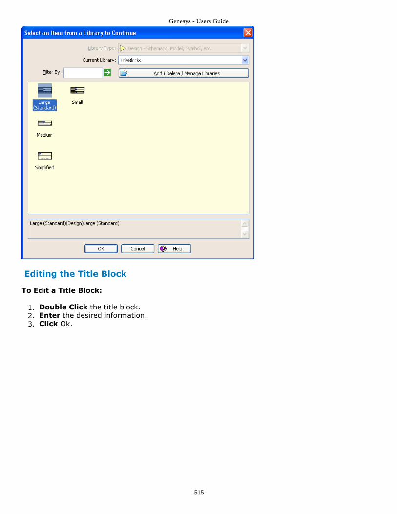
Genesys - Users Guide
515
Editing the Title Block
To Edit a Title Block:
Double Click the title block.1.Enter the desired information.2.Click Ok.3.

Genesys - Users Guide
516
Item - Name or titles of information.
Note: These titles can only be changed on a custom title block symbol.
Text - The actual text string to be drawn in the title block.Scale X & Y - Scales the title block. For example, 0.5 is half-size.Draw semi-transparent - When checked draws a faded title block.
HintFor Advanced users: An equation can be used for the text. For example, if the workspace contains anequation block with a text variable named CompanyName, place =CompanyName in the Text field ofthe title block. The leading = sign indicates that the text string is actually an expression. When the titleblock is drawn, the variable will be evaluated and the result will be displayed in the title block.
Creating a Custom Title Block
The easiest way to create a custom title block is to start with an existing one.
Open up the Library Selector.1.Set the Library Type to Design.2.Change the Current Library to TitleBlocks.3.Double click on the title block to be modified.4.
Note: This will add the title block as a schematic symbol on the workspace tree.
Edit title block symbol as needed, using annotations:5.The text annotation Name property will be used as the Item Name. The ShowName option must be checked in this annotation dialog box to see this name onthe schematic.The text annotation Enter 1 or more lines of text property will be the textvalue of the field that appears in the title block.
HintFor best results, only use 1 line of text and keep it fairly short.
Images, like a company logo, or any other annotation can be placed on the

Genesys - Users Guide
517
custom symbol.Save the workspace.6.On workspace tree, right-click the symbol and use "Copy To" to place the symbol7.in a new (or existing) library.To use your new custom title block on a schematic, use "Add Title Block..." and8.select the custom title block from the library it was saved in.
Annotating Schematics
The Annotation button ( ) on the Schematic toolbar gives you access to theAnnotation toolbar.
The Annotation toolbar provides tools like lines, circles, and text that you can use to pointout details of interest on a schematic, draw a box around a group of components, etc.
HintDouble-click a text annotation to set the horizontal and vertical justification (text alignment).
HintFor Advanced users: An equation can be used for the text. For example, if the workspace contains anequation block with a text variable named CompanyName, place =CompanyName in the Text field ofthe title block. The leading = sign indicates that the text string is actually an expression. When the titleblock is drawn, the variable will be evaluated and the result will be displayed in the title block.
Text annotations can display model and parameter info when used within a customsymbol. This is implemented via macro-text-substitution. When symbol text is drawn on aschematic, the displayed text is modified prior to output. For example, Name=%Model%would be displayed as "Name=Resistor" on a symbol using a resistor model. Therecognized macro strings are:
%Des% - Displays the part's designator.1.%Model% - Displays the name of the model attached to the part.2.%MODEL% - Displays the model name in UPPERCASE.3.%ParameterName% - Displays the value of the specified model parameter4.attached to the part.
Adding Text
Text can be placed directly on a schematic.
To add text:
Click the Annotation button ( ) to display the Annotation toolbar.1.
Click the Text button ( ).2.Click in the Schematic window where you want to place the text.3.Type the text into the Enter 1 or lines of text field.4.
Specifying Schematic Part Layout Options
Often in RF circuits, you want to model packaging or component parasitics. You do this byplacing lumped parts in series or parallel with the actual part. However, you do not want

Genesys - Users Guide
518
these parts to display in the layout.
To prevent a schematic part from displaying in a layout:
Double-click a part in the schematic and click the Advanced Options button.1.Click the Layout tab.2.Click an option. For capacitors, select Replace Part with Open. For inductors and3.resistors, select Replace Part With Short.Click OK.4.
Using DisCosInserting discontinuities such as bends and tees for distributed parts is simplified withparts called DisCos. These small symbols are easily added to any schematic that usesmicrostrip lines or similar distributed parts. This avoids the need to manually add thesemodels by disconnecting the parts, selecting the discontinuity from toolbars, reconnectingthe parts, and defining parameters.
Using Distributed Parts
You can use distributed parts such as microstrip lines as schematic objects. Placedistributed parts in a schematic the same way as lumped parts such as resistors andcapacitors. Also, it is now easier to insert discontinuities such as bends and tees in aschematic.To add a microstrip:
Click the New Item button ( ) on the Workspace Tree toolbar and select With a1.Schematic from the Designs menu.
Click the Microstrip button ( ) on the Schematic toolbar.2.
Click the Microstrip Line button ( ) on the Microstrip toolbar, and then click in3.the Schematic window to place the part.Press the spacebar to repeat the selection.4.Click the right terminal of the first part to place the second part.5.Add input and output ports.6.Continue to add microstrip parts as shown below. Double-click each part to enter7.values (width and height).

Genesys - Users Guide
519
To add discontinuities:
Right-click the node in the schematic that connects the three line segments.1.Select Add Tee DisCo. A small symbol appears. This DisCo (discontinuity) functions2.the same as the tee part from the Microstrip window.Right-click the bend.3.Click the Chamfered Corner DisCo check box.4.Place an End DisCo on the open terminal. The resulting schematic is shown below. 5.
Note: For this example, clear the Absorb DisCos check box to preserve circuit response whenpossible. This option adjusts the line lengths connected to each DisCo and is useful if the design isoptimized.
Reviewing Rules for Using DisCos
The following rules apply for using DisCos:
DisCos can connect only to a node with one or more transmission lines.All connected transmission lines must be the same type and use the same substrate.The number of transmission lines connected to a node is one factor in determiningthe DisCos to apply.

Genesys - Users Guide
520
Numberof Lines
Possible DisCos
1 End Effect
2 Step or Bend
3 Tee
4 Cross
A bend is inserted at a node where two transmission lines meet at a right angle in aschematic.A step is applied at a node between two transmission lines of unequal widths.
Reviewing Tips for Using DisCos
The following tips apply for using DisCos:
When generating the original schematic, be aware that the orientation of partsaffects the application of DisCos. For example, transmission line parts meeting atright angles result in a "bend" DisCo when converted. The same orientation isimportant when layouts are generated from the schematic.If more than one line type is used in a schematic, you can still use DisCos by right-clicking each node. Note that DisCos can connect only to a node with one of moretransmission lines, still applies.The option of preserving circuit response when possible is useful if the circuitresponse is already optimized. This minimizes the need for major changes incomponents to compensate for the discontinuities.
Using SubstratesIf your schematic contains any parts that use a substrate (such as microstrip, slabline,stripline, coax, and waveguide), you must add one or more substrates to your designbefore you can analyze it. Genesys lets you add and change substrates using theSubstrate Properties window. You can also add a substrate from the Genesys library or auser library.
Adding and Changing Substrates
A substrate is required whenever a physical component is used in a schematic or a netlist.Components that require substrates are:
Coaxial (users)Microstrip (users)Slabline (users)Stripline (users)Waveguide (users)
You can also use substrates to provide metal and substrate characteristic information toEMPOWER by selecting the substrate name in the EMPOWER Layer table.To add a new substrate:
Click the New Item button ( ) on the Workspace Tree toolbar and select Add1.Substrate.Type substrate and metal layer parameter values.2.Click OK.3.
To add a library substrate:

Genesys - Users Guide
521
Click the New Item button ( ) on the Workspace Tree toolbar and select From1.Library.Select the Substrate type of library2.Open a substrate library3.Locate the substrate you want to add, and then click Open or double-click the4.substrate.
To change substrate properties:
Right-click the substrate in the Workspace Tree and select Properties.1.Make the changes you want.2.Click OK.3.
To change substrate properties of ALL the parts in a schematic (to use a tunedvariable, etc.):
Click the New Item button ( ) on the Workspace Tree toolbar and select From1.Library.Select the Script type of library2.Add the ReplaceSubstrates script to your workspace3.Double-click to open the script, edit it according to the instructions in the script.4.Run the script.5.
Substrate Parameters for Microstrip and Stripline
For an overview of substrate parameters, see Substrate Parameters for Microstrip andStripline (users).
Substrate Parameter Tables
For a listing of substrate parameter tables, including:
Loss TangentMetal ThicknessRelative Dielectric ConstantsRelative PermeabilityResistivitySurface Roughnesssee Substrate Parameter Tables (users).

Genesys - Users Guide
522
Substrate Parameter Tables Loss TangentThe dielectric loss tangents of some common materials are:
Material tanD at 100 MHz tanD at 10 GHz
Air 0.0 0.0
Polyolefin, irradiated 3E-4 3E-4
PTFE (Teflon) 2E-4 1.5E-4
RT/Duroid 5880, PTFE microglass 5E-4 9E-4
Teflon, glass microfiber 5E-4 9E-4
Teflon, woven quartz 6E-4 6E-4
Teflon, woven glass 1.5E-3 2E-3
Polystyrene, cross linked 2E-4 7E-4
Polystyrene, glass microfiber 4E-4 2E-3
Quartz, fused 2E-4 6E-5
G10 Epoxy glass 8E-3 No Data
Pyrex glass 3E-3 7E-3
Alumina, 99.5% 1E-4 1E-4
RT/Duroid 6010.5, PTFE ceramic 2E-3 2.3E-3
The dielectric loss tangents for some materials commonly used in coaxial cables are:
Material tanD at 100 MHz tanD at 3 GHz
Air 0.0 0.0
Teflon 2E-4 15E-4
PolyEthylene, DE-3401 2E-4 3.1E-4
Polyolefin, irradiated 3E-4 3E-4
Polystyrene 1E-4 3.3E-4
Polyvinal formal (Formvar) 1.3E-2 1.1E-2
Nylon 2E-2 1.2E-2
Quartz, fused 2E-4 6E-5
Pyrex Glass 3E-3 5.4E-3
Water, distilled 5E-3 1.6E-1
This data is for solid materials. Foamed materials have lower loss tangents. These data are approximate.Consult manufacturer for critical applications.
Metal ThicknessThe thickness of the conductor metalization for planar structures. The algorithms formicrostrip are most accurate for thin metalization, but both loss and Zo are corrected forthickness.
For stripline, the algorithms are more accurate to thicker metalization. Thickness to 0.1*bor to the width is permissible.
Commonly used thicknesses:

Genesys - Users Guide
523
Metallization Type Thickness (mm) Thickness (mils)
½ ounce copper 0.018 0.71
1 ounce copper 0.036 1.42
2 ounce copper 0.072 2.83
Relative Dielectric ConstantsEr is the substrate or dielectric constant, relative to free space. Following are constants ofsome common materials:
Material Dielectric Constant
Air 1.0
Alumina, 99.5% 10
G10/FR4 Epoxy glass 4.8 (varies)
PolyEthylene, DE-3401 2.26
Polyhexamethyleneadipamide (Nylon) 2.9
Polyolefin, irradiated 2.32
Polystyrene 2.53
Polystyrene, cross linked 2.53
Polystyrene, glassed cross linked 2.62
PolyTetraFluoroEthylene (Teflon) 2.10
Polyvinal formal (Formvar) 2.8
PTFE, glass microfiber 2.35
PTFE (Teflon) 2.10
PTFE, woven glass 2.55
PTFE, woven quartz 2.47
Pyrex glass 4.84
Quartz, fused 3.8
RT/Duroid 2.20
RT/Duroid, PTFE ceramic filled 10.5
Water, distilled 77
Foamed materials have lower dielectric constants. These data are approximate; consult manufacturer forcritical applications.
Relative PermeabilityUr is the substrate permeability, relative to free space. Most line types do not allowsubstrates or dielectrics with magnetic properties.
ResistivityRho is the lines metalization resistivity relative to copper.
Some common values are:

Genesys - Users Guide
524
Material Resistivity Relative to Copper
Copper, annealed (1.7e-8 ohm meters) 1.00
Copper, hard drawn 1.03
Silver 0.95
Gold 1.42
Aluminum 1.64
Tungsten 3.25
Zinc 3.4
Brass 3.9
Cadmium 4.4
Nickel 5.05
Phosphor-bronze 5.45
Platinum 6.16
Stainless Steel, 18-8 52.8
Surface RoughnessSr is the metalization surface roughness, using the current units.
Conductor losses increase with larger values of surface roughness. Approximate values forcopper PWB surface roughness:
Electrodeposited Copper Sr value (mm) Sr value (mils)
½ ounce 0.0019 0.075
1 ounce 0.0024 0.094
2 ounce 0.0029 0.114
Rolled Copper Sr value (mm) Sr value (mils)
½ ounce 0.0014 0.055
1 ounce 0.0014 0.055
2 ounce 0.0014 0.055

Genesys - Users Guide
525
Substrate Parameters for Microstripand Stripline Microstrip Overview
The substrate height "H" is the entered value in the Substrate properties field "(Height)Substrate Height"
More information regarding substrate properties can be found in the Substrate Parameter Tables (users)section.
Stripline Overview
If the Stripline will be manufactured by purchasing two substrates, each substrate willhave H/2=H' height. Length "L" is the length of the transmission strip. This dimension is"looking into the page" toward the "z" axis.

Genesys - Users Guide
526
More information regarding substrate properties can be found in the Substrate Parameter Tables (users)section.
Parameter List
Er Dielectric Constant of substrate
Ur Magnetic Constant of substrate
Tand Loss Tangent of substrate
Rho Resistivity of substrate
Thick Metal thickness
Sr Metal roughness
Height Substrate height (top ground place to bottom ground plane)

Genesys - Users Guide
527
Using S-Parameters in GenesysThis section shows how S-Parameter data can be incorporated into Genesys designs andexported to other programs.
S-Parameters are commonly used in RF circuits to represent incident and reflectedtraveling waves. S-Parameters are created by a linear simulation and are generallyavailable from component manufactures. Several libraries of S-Parameter data ship withGenesys. S-Parameters in Genesys are imported and exported in the Touchstone format.
ContentsCreating S-Parameter Data (users)File Based S-Parameters (users)Displaying S-Parameter Data (users)Physical S-Parameters (users)Touchstone Format (sim)
Creating S-Parameter DataCreate the schematic for which the S-Parameter data will be represented1.Add a linear analysis and point it to the desired schematic2.Set the frequency range and step size of the linear analysis to the desired resolution3.of the S-Parameter dataRun the linear analysis4.Export linear analysis data as a S-Parameter file5.
Using S-Parameters in a Simulation
The use model for S-Parameters manually imported into the workspace versus file basedS-Parameter is slightly different. The model used in the schematic determines how the S-Parameters will be managed.
Displaying S-Parameter DataThe easiest way to display S-Parameter data is to open up the S-Parameter dataset andthe right click on the S variable. Then select Create Table or Graph and the type ofgraph. The data will automatically be displayed.
Files with No Noise ParametersNoise parameters can be added to an S-Parameter file so noise characteristics of activedevices can be simulated. For passive devices the noise characteristics are determineddirectly from the S-parameters so noise parameters are not needed.
CautionIf an S-Parameter file represents an active device no noise will be created and a warning will be displayed.
File Based S-ParametersFile based S-Parameter import the S-Parameters from a file into a dataset providingsimulation cache. This dataset is used when reloading the workspace to re-cached thedata. If the dataset is deleted the S-Parameters will be re-imported the next time asimulation needs the data.

Genesys - Users Guide
528
Place a S-Parameter file based part in the schematic (1-port (part), 2-port (part), or1.N-port (part). This can be done from the Linear Toolbar or the Part SelectorDouble click the part to bring up the part properties2.Click the Browse button to browse to the S-Parameter file3.Add an analysis and point it to the desired schematic4.Run the analysis5.
Physical S-ParametersS Parameters can be taken or formed in such a way that they represent non physical partslike negative resistors. Realistic real world answers only come when S-Parameters arephysical. If S-parameters are physical, then the corresponding Y-parameters will meet allof the following requirements:
The real part of every diagonal entry must be positive. i.e. Real.Yp[i,i] > 01.The real part of every non-diagonal entry must be negative. i.e. Real.Yp[i,j] < 02.where i is not equal to jThe absolute value of the row real summation, excluding the diagonal, must be less3.than real value of the diagonal in that row. i.e. abs ( sum( Real.Yp[i,j] ) ) <Real.Yp[i,i] where i is not equal to jThe absolute value of the column real summation, excluding the diagonal, must be4.less than the real value of the diagonal in that column. i.e. abs ( sum( Real.Yp[i,j]) ) < Real.Yp[j,j] where i is not equal to j
Note: It is assumed the Y parameters are in Real _ j Imaginary format.
Examples:Here are some typical Y-parameters (which is converted from S-parameters):

Genesys - Users Guide
529
The Y parameter matrix for F = 3000 is:
0.077 - j0.122 -0.078 + j0.123
-0.078 + j0.123 0.078 - j0.121
This matrix meets items 1 and 2 but not 3 and 4, because abs( Real.Y[1,2] ) >Real.Y[1,1] or abs( Real.Y[2,1] ) > Real.Y[1,1], so these S parameters are non physical.

Genesys - Users Guide
530
Sub-Network ModelsA sub-network model is used to abstract a model or group of models to something easierto use and manage from a users perspective. This type of model hides implementationdetails that may confuse the user or distract from the readability of a simulation topology.
For example, a user may want to simulate the effects of a non-linear filter. Models existfor filters and non-linear blocks. However, there is no non-linear filter model. A new sub-network model can be created out of the two existing models. The parameters from thesetwo models can be abstracted to only reveal parameters that user would be interested inentering for this type of sub-network model.
The abstraction of the Sub-Network model in Genesys is really an object called a design.The Sub-Network model is really a design object with the following attributes:
PartListSchematicEquationsParametersNotes
All of these attributes are interrelated except for the Notes which serve as documentationor help for the Sub-Network model.
ContentsRoles of Sub-Network Model Attributes (users)Creating Parameterized Sub-Network Model (users)Run-time Hierarchy (users)
Creating a Parameterized Sub-Network ModelThere are two different ways to to create a sub-network model in Genesys. One is by
clicking on the New Item button ( ) on the Workspace Tree toolbar. The other is byright clicking on a folder in the workspace tree.
Method 1 - Clicking on the New Item Button
Click the New Item button ( ) on the Workspace Tree toolbar1.Select the 'Designs >' submenu2.Now select 'Add User Model...'3.This model will be added under the folder that last selected in the workspace tree4.
Or
Method 2 - Right Clicking on a Workspace Folder

Genesys - Users Guide
531
Right click on a folder in the workspace tree to bring up the right click menu.1.Select the 'Add >' submenu.2.Select the 'Designs >' submenu3.Now select 'Add User Model...'4.The design will be added under the folder that was initially right clicked5.
NoteIf you create the new design in the wrong folder, simply drag it to the folder of interest.
Entering User Parameters
Add new parameters by clicking the Add Parameter button.1.Copy selected parameters (from the parts in the design) into the list by clicking the2.Copy Parameters button. A selection dialog box is displayed. Select individualparameters (to copy from the base design) by placing a checkmark beside eachparameter you wish to copy. Then click OK.Tip: This is the recommended way of adding parasitics (etc.) to an existing part (a"user model").Delete unwanted entries with the Delete Selected Parameter button.3.
Name - The name of the parameter.Description - A short description of the parameterDefault Value - The normal, standard value for this parameterUnits - The units-of-measure for this parameterTune - Is it normally tuned?Show - Is it normally shown on a schematic?Initially Use Default - Should the Default value be used when the part is placed ona schematic?Validation - Usage rules that determine if a parameter value is valid and in-range.

Genesys - Users Guide
532
See details below.Hide Condition - Dependence of the activity and visibility of the parameter onvalues of other parameters of the design. See details below.
Validation Types
Type Comment
Floating pointnumber
1.0, 1e-6, etc. are valid entries
Warn if negative Posts a warning if the value is < 0
Warn if non-positive
Posts a warning if the value is < 1
Positive integer Only numbers like 1, 2, 3, ... are allowed
<None> No validation will be performed
Text The parameter is a string; any text is valid
Warning Always generates a warning
Error if negative Posts an error if the value is < 0
Error if non-positive
Posts an error if the value is < 1
Error Always generates an error
Filename Brings up a browse button for file selection as well option for manual a text entry
Integer Any integer value
Complex number Complex number in RI MathLang syntax, e.g. X + j*Y. Real and integer values supportedby default
Integer array Fully defined MxN array of integers with comma delimited columns and semi-colondelimited rows
Floating pointarray
Fully defined MxN array of integer or real numbers with comma delimited columns andsemi-colon delimited rows
Complex array Fully defined MxN array of integer, real or complex numbers with comma delimitedcolumns and semi-colon delimited rows
Enumeration Allows definition of arbitrary user-defined labels and options for assigning values to theparameter of interest
NoteAn array parameter may be specified as a scalar number without any delimiters as in MyArray0=2.345. Itmay be a one-dimensional vector as in MyArray1=[2, 3, -4].Two-dimensional arrays are specified row over column as MyArray2=[1, 2, 3; 4, 5, 6] where the firstthree parts form the first row.Higher dimensions are created by appending nested versions of 2-D representations separated by semi-colons e.g.MyArray3=[[1, 2; 3, 4; 5, 6]; [-1, -2; -3, -6; -5, -4]].This is a 3-D array consisting of 2 separate 3x2 2-D arrays such that matrix size is 2x3x2.
Using enumerated parameters
The process of defining an enumerated parameter starts with the selection of thisvalidation type followed by selection of the context sensitive Edit Enumeration buttonwhich appears adjacent to the other parameter editing buttons. Clicking this button willinvoke the Enter List of Enumerated Parameter Values dialog box.

Genesys - Users Guide
533
It is possible to choose a pre-defined enumeration template by selecting the library andenumeration name. Customizations can be performed by clicking the New Enumerationbutton which is transformed into a Copy From ... button to allow graphical selection froman existing library, or a newly created enumeration library, name and description.
Names and states of manually created enumerations or modifications of existingenumerations can be directly entered into the table and organized using the Add,

Genesys - Users Guide
534
Remove, Up and Down buttons.
Upon accepting the enumeration list, the corresponding drop-down menu is created underthe Default Values column for this parameter in the main Parameter tab. Note that thefirst entry of the enumeration table will be treated as the initial default value regardless ofthe state number associated with it. In this example, the first entry was 1:InvertingBehavior, which despite its state number being 1, not 0, was picked as the default in theParameters main tab. The user can set a different default state prior to leaving this tab.
Setting Hide Condition
The final column of the Parameter entry table allows the user to set up Boolean conditionsfor establishing a clean functional approach to parameter definitions - by allowingconditional deactivation and hiding of parameters.MathLang syntax can be used to set up conditions of indivisibility of one parameter basedon current values assigned to other parameters.
One example is shown in the Amplifier part of the Algorithm Design library. This built-incomponent has a total of 11 parameters as shown in the model view which can beimported from the library into any workspace.
Observe that the parameters TOIout, dBc1out, PSat, GCSat, RappS and GComp all haveconditions of inactivity defined based on the value of GCType. For instance, TOIout is to behidden and its assigned value ignored if GCType is not in the set {1, 3, 4, 6}. Thecorresponding behavior can be observed when placing an instance of the part on aschematic and invoking its Properties dialog box.
When GCType is selected to be a member of the above mentioned set, e.g. to3:TOI+1dBc, the TOIout parameter is displayed and enabled for editing.

Genesys - Users Guide
535
Setting GCType to a non-member e.g. 2:1dBc hides the parameter from view even on theProperties table.

Genesys - Users Guide
536
Note
Defining Hide Conditions refers strictly to the table view of parameters and not the visibility of selectedparameters on the schematic. Parameters that are hidden by condition are barred from schematic displayeven if they had the Show button checked prior to concealment.
As you simulate this design in the workspace, the default parameter values will be used inthe simulation. When you use this design as a model in a part, the part parametersoverride these default parameter values.
Roles of Sub-Network Model AttributesParameters - These are the parameters the user sees when entering values for thismodel.Equations - These are commonly used to manipulate data entered by the users to aformat needed by models that appear in the schematicSchematic - This shows how existing models are visually and electrically connectedtogether and their relationships with each other. The model parameters in theschematic can also use the top level parameters as well as any variable created inthe equation block.PartList - This shows connectivity and part information in a table format.Notes - This is used for documentation or help for this sub-network.
Run-time Hierarchy - How Parameters get passedWhen a simulation is run, a model tree is instantiated that corresponds to the topology ofthe network you are simulating. This is called the run-time hierarchy. In contrast, whenyou are editing designs in the workspace, you are working in design-time. The differencewill become apparent shortly.

Genesys - Users Guide
537
Each part in your top level design references a model, and an instance of that model iscreated and set as a "child" of the top-level design when a simulation is run. If one ofthese children corresponds to a subnetwork model, then each model inside thesubnetwork design is instantiated as well, recursively. It is easy to see why this sort ofinstantiation is necessary - you can have two parts in your top-level design that point tothe same model, and they may have different values for their parameters.
Suppose we have a workspace as shown here (ie. this is the design-time hierarchy):
and suppose that TopLevel contains 2 instances of SubNetwork, ie. TopLevel has 2 partscalled Part1 and Part2 whose models are both "SubNetwork". When you run a simulationon TopLevel, the following run-time model hierarchy is constructed:
Note that the Equations and Parameters of TopLevel are visible to the model instances ofPart1 and Part2, but only at run-time!
It is important to note that when you are looking at the design called SubNetwork (ie. indesign-time), and in its schematic you are using parameters defined in the Parameters tabof SubNetwork, the values you see at design-time will correspond to the "Default" valuesof the parameters as defined in the Parameters tab. This is because you are editing theModel called SubNetwork, but that model can be instantiated many times in your top-levelnetwork, and each instance can have different values for the parameters. Since you areediting the design-time model, it has no way of knowing what the values passed to it willbe at run-time, and thus just shows the default values that are defined at design-time.
Genesys - Users Guide
538
SweepsSweeps are used to create analysis results that are functions of a parameter tuned atseveral values. A sweep is an evaluation object that controls a specific analysis. It alsocontains a single tuned parameter that is swept across a range of values specified by theuser.
Once a parameter is made tunable (part parameter 'Tune' checkbox has been checked ora question mark '?' has been placed in front of the equation value) it can be selected inthe Parameter Sweep Properties dialog box. The user specifies hard Start and Stopvalues as well as the number of swept points.
The number of swept points can be specified in 1 of 4 ways:
Linear: Number of PointsLog: Points / DecadeLinear: Step SizeList
Once the analysis has been selected and the swept parameter has been defined thesweep will tune the parameter to the first point, run the analysis, and then save the datain a sweep dataset. The swept parameter is tuned to the next value, the analysis is re-ranand the new data will be appended to prior values. This process repeats until the lastswept point is reached.
HintRemember, an analysis and tuned variable must exist in the workspace before a sweep can be created.
NoteA sweep can control another sweep. Sweeps are also considered an analysis and will appear in theAnalysis to Sweep list. A good example of this are IV curves for a transistor. One sweep will point to thetransistor circuit and sweep its supply voltage the other sweep will control the first sweep as the biascurrent is swept across its range.
NoteFor additional information on sweeps in Spectrasys see Sweeps of a Path (sim).
ContentsGetting Started with Parameter Sweeps (users)Parameter Sweep Properties (users)Understanding Swept Data (users)

Genesys - Users Guide
539
Understanding Swept DataThe following figure shows the dataset for a modified version of the Getting Started withParameters Sweeps (users) example. This example was modified to reduce the number oflinear simulation points from 101 to 6 so the results could be seen in a single figure.
In summary, there is a linear simulation of simple LC low pass filter over 6 frequencypoints (0, 30, 60, 90, 120, and 150 MHz). A sweep has been created that tunes the filterinductor parameter L across 6 values (100, 120, 140, 160, 180, and 200 nH).
Column Name Description
Index Row number in the table.
F (MHz) First independent variable of swept data. In this example, this is the frequency range of thelinear analysis. It is repeated for each tuned value of the swept parameter.
L1_L_Swp_F(nH)
Second independent variable of swept data. In this example, this is the tuned value of theinductor parameter L at each frequency point of the linear analysis.
|S21| (dB) Dependent variable for each tuned parameter value (inductor) at each frequency.
NoteThe independent variables (in this example F and L1_L_Swp_F) are also stored in the dataset.

Genesys - Users Guide
540
HintFor additional information on indexing into sweeps see Using Engineering Language (users) or Using MathLanguage (users).
Getting Started with Parameter SweepsThe steps for creating a parameter sweep are:
Create a schematic (or design)1.Add an analysis2.Make a variable tunable3.Create a parameter sweep4.Run the sweep5.Plot the data6.
Create a Schematic
A simple Lowpass filter can be created as follows (the schematic is named LPF_Sch):
NoteSee Creating a Simple Schematic (users) in the User's Guide for details on schematic creation.
Add an Analysis
Create the linear analysis

Genesys - Users Guide
541
Set the values as shown in the above dialog
NoteSee the Analysis (users) section in the User's Guide for details on creating an analysis.
Make Variables Tunable
There are two ways to make variables tunable:
Through part properties1.As an equation variable2.
Method 1 - Part Properties
Check the Tune checkbox for the parameter to be tuned
Method 2 - Equation Variable
Create the variable in an equation block and place a ? before the value

Genesys - Users Guide
542
HintRemember to set the parameter value to the equation variable name to link the equation to the partparameter. In this example the variable name Inductor would be used for the part parameter Value of Linstead of 130.
Create the Parameter Sweep
Add a new sweep to the workspace tree by right clicking on a folder and selectingAdd Sweep from the submenus.
Set the sweep properties as follows:

Genesys - Users Guide
543
Run the Sweep
The sweep can be ran in one of two ways:
From the Play button on the main toolbarFrom a right click menu selection on the workspace tree
Method 1 - Main Menu Play Button
HintThe asterisk * next to the analysis name indicates the analysis data is out of date.
Method 2 - Workspace Right Click Menu

Genesys - Users Guide
544
Plot the Data
Add a graph to the workspace tree
NoteSee Creating Graphs (users) in the User's Guide for additional information.
The swept results are shown below

Genesys - Users Guide
545
NoteGraphs that contain swept data display a trace for each swept value.
Parameter Sweep Properties

Genesys - Users Guide
546
Name Description
Sweep Name Name of Sweep Evaluation
Analysis to Sweep Analysis used for the parameter sweep. The selected analysis will be recalculatedfor each different value of the swept parameter.
Parameter to Sweep Parameter that gets changed to create the sweep. All parameters defined astunable are available to be swept.
Output Dataset Dataset file in which the data is saved. If not specified, the dataset name will bethe name of the analysis with "_Data" appended.
Description Description of the evaluation being run. For documentation purposes only, nototherwise used by Genesys.
Calculate Now Run the evaluation. Always runs the analysis, regardless of whether or not anychanges were made.
Propagate All VariablesWhen Sweeping
User created variables in the source dataset will be swept and aggregated intothe sweep dataset.
Show Long ParameterName
Display the full parameter name (with path) in case you have multipleparameters with the same short name (such as C1.C).
Factory Defaults Reset all values to their default
Parameter Range Start. The lower bound (minimum frequency) of the sweep.
Stop The upper bound (maximum frequency) of the sweep.
Unit of Measure Unit of measure used for the evaluation
Type of Sweep Linear: Number of Points. Number of points in entire sweep.
Log: Points/Decade Number of points in each decade of the sweep.
Linear: Step Size (MHz) Allows specification of start and stop frequencies, and space between points.
List of Frequencies (MHz) Allows the explicit specification of analysis frequencies. These points are enteredinto the List of Frequencies box separated by spaces.

Genesys - Users Guide
547
TablesTables provide text-based tabular output instead of graphical output. There is only onetype of table in Genesys. You can place any measurement in a table. Change theproperties of a table using the Table Properties window.
Use Ctrl_MouseWheel to zoom in and out on tables.
Any type of alpha-numeric data (such as S-parameters) may be displayed in a table:
ContentsCreating Tables (users)Table Toolbar (users)
Creating TablesThe easiest way to create a new graph is using the Instagraph Feature (users).The easiest way to add an arbitrary measurement to an existing table is via theMeasurement Wizard (users).Tables can also be created manually:
Click the New Item button ( ) on the Workspace Tree toolbar and select Add1.Table.Enter the measurements you want to display in the Table Properties dialog..2.
Click OK.3.(note that the Independent Variable for PPORT2 in the Snap dataset was set to thesame as PPORT[2] to remove a second Freq column)

Genesys - Users Guide
548
The Label entry determines the column labels.
If the data is complex it will often display as dB or magnitude by default. To see the fullcomplex data select a format from the Complex Format column.
If you want to print a table, copy it to a notes object by using the Copy To Notes right-click menu entry. This copies the headings and data into an HTML table which you canthen copy to Word or other HTML editor or you can just print the Notes. Modify the Notesmanually to change fonts or formatting.
New Right-click in the table header to get a popout menu that lets you turn offcolumns.

Genesys - Users Guide
549
TemplatesTemplates are a very convenient way to get started quickly with a new design. They giveyou a complete circuit as your starting point. You can also modify templates for yourspecific program. Many templates are included with Genesys, and you can easily add yourown.
Selecting a Genesys Template (users)Reviewing the Genesys Templates (users)
Selecting a Genesys TemplateThe Default.wsx template is automatically loaded whenever a new workspace is created.You can use it or select a different Genesys template.
To select a template to always start with:
Click Tools on the Genesys menu and select Options.1.Click the Startup tab.2.
Click the button: Use the Default Workspace as a Starting Point3.Click the folder button and select a template.4.Click Open, and then click OK.5.
The default templates are workspaces stored in a folder at (default) C:\programfiles\Genesys20xx.xx\Template. You can place your own template workspaces there, as well.
To select a template once:
Click the Start Page button ( ) on the Genesys toolbar.1.

Genesys - Users Guide
550
In the templates area double-click a template name, such as "Linear Simulation".2.
Reviewing the Genesys TemplatesThe table below lists all of the workspace templates included in Genesys.
File Name Description
Default.wsx A blank schematic.
Linear Simulation.wsx A linear analysis template.
Nonlinear Simulation.wsx A nonlinear analysis template.
Oscillator Template.wsx An oscillator analysis template
Phase Noise Template.wsx A workspace which helps determine the phase noise of an oscillator.
SynthesisDefault.wsx The base synthesis template, used by Filters, WhatIF, etc.
System Template.wsx A System Analysis (Spectrasys) template
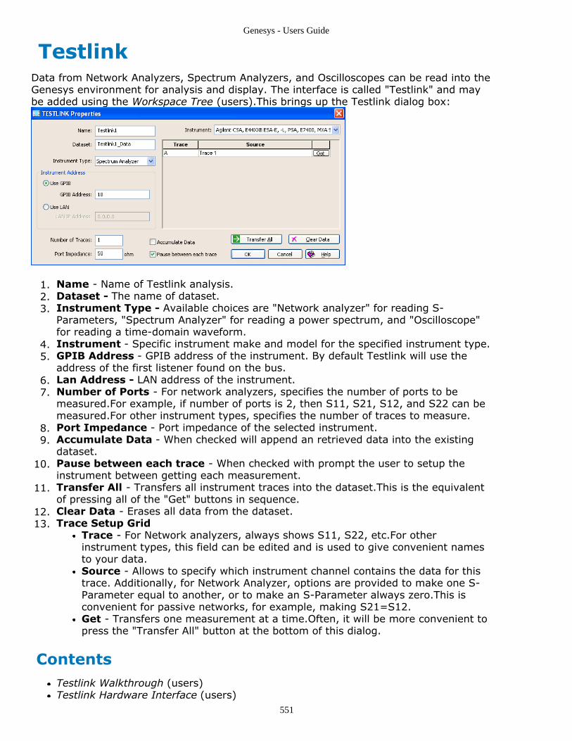
Genesys - Users Guide
551
TestlinkData from Network Analyzers, Spectrum Analyzers, and Oscilloscopes can be read into theGenesys environment for analysis and display. The interface is called "Testlink" and maybe added using the Workspace Tree (users).This brings up the Testlink dialog box:
Name - Name of Testlink analysis.1.Dataset - The name of dataset.2.Instrument Type - Available choices are "Network analyzer" for reading S-3.Parameters, "Spectrum Analyzer" for reading a power spectrum, and "Oscilloscope"for reading a time-domain waveform.Instrument - Specific instrument make and model for the specified instrument type.4.GPIB Address - GPIB address of the instrument. By default Testlink will use the5.address of the first listener found on the bus.Lan Address - LAN address of the instrument.6.Number of Ports - For network analyzers, specifies the number of ports to be7.measured.For example, if number of ports is 2, then S11, S21, S12, and S22 can bemeasured.For other instrument types, specifies the number of traces to measure.Port Impedance - Port impedance of the selected instrument.8.Accumulate Data - When checked will append an retrieved data into the existing9.dataset.Pause between each trace - When checked with prompt the user to setup the10.instrument between getting each measurement.Transfer All - Transfers all instrument traces into the dataset.This is the equivalent11.of pressing all of the "Get" buttons in sequence.Clear Data - Erases all data from the dataset.12.Trace Setup Grid13.
Trace - For Network analyzers, always shows S11, S22, etc.For otherinstrument types, this field can be edited and is used to give convenient namesto your data.Source - Allows to specify which instrument channel contains the data for thistrace. Additionally, for Network Analyzer, options are provided to make one S-Parameter equal to another, or to make an S-Parameter always zero.This isconvenient for passive networks, for example, making S21=S12.Get - Transfers one measurement at a time.Often, it will be more convenient topress the "Transfer All" button at the bottom of this dialog.
ContentsTestlink Walkthrough (users)Testlink Hardware Interface (users)

Genesys - Users Guide
552
Testlink Registration (users)
Testlink Hardware Interface
Set-up
Connect PC to measurement instrument, such as an oscilloscope, network analyzer,1.or spectrum analyzer using a GPIB card or RS-232 port. A partial list of supportedinstruments is found below. There is no limit to the number of instruments. Theinstruments can be daisy-chained or connected in a "star" configuration. Verify theproper operation of the PC / instrument communication using the software suppliedby the interface card manufacturer. A list of available GPIB interface cards is alsoprovided.Load the Genesys software on the PC with Testlink option. Then insert a Testlink icon2.on the workspace tree and transfer the data into the Genesys workspace. Thencompare simulated versus measured data or use the data as models in largersimulations. See the Testlink walk-through for details on using Testlink data insimulations, equations, and other analyses.
Hardware Requirements
PC Requirements:
Minimum System Requirement: Same as Genesys
GPIB card:
National Instruments: type PC-IIA, PC-AT, PC-PCMCIA, PC-USBAgilent/Hewlett-Packard: HP82335, HP82340, HP82341, HP82350ComputerBoards Inc.: GPIB card, type ISA-GPIB, ISA-GPIB/LC, ISA-GPIB-PC2A, PCI-GPIB, PCM-GPIBines: GPIB-PCMCIA, GPIB-PCI card
TEST LINK can also use RS-232 port if the instrument supportsit.
Network Analyzers:
Advantest: R3753H, R3764/65/66/67H, R3765/67GAgilent: E5061/62/70/71A/B ENA Series, E835XA/B, E836XA/B PNA Series, E4991Impedance AnalyzerAnritsu: Wiltron 360 Series, Wiltron 371/372/373xxA Series, MS462XX Series,MS3401A/B, MS4630B, 54xxA / 541xxA / 56100A Scalar Analyzers, Site Master SxxxA/BHewlett-Packard: HP 35660 Dynamic Signal Analyzer, HP 35665/35670A DynamicSignal Analyzer, HP 3577A, HP 3589A (Network Analyzer Mode), HP 4145A/BSemiconductor Parameter Analyzer, HP 4155/56 Semiconductor Parameter Analyzer, HP4192 Impedance Analyzer, HP 4194A Impedance Analyzer, HP 4195 (Network AnalyzerMode), HP 4280 Capacitance Meter, HP 4284A Precision LCR Meter, HP 4291A/BImpedance Analyzer, HP 4294A Impedance Analyzer, HP 4352B VCO / PLL SignalAnalyzer, HP 4395A Network/Spectrum/Imped Analyzer, HP 4396A Network/SpectrumAnalyzer, HP E5100A/B HP 8510, HP 8711-14B/C Series VNA, HP 8720 series VNA (8753E,8720, etc.), HP 8751 Series VNA, HP 8752A, 8753A/B/C, HP 8756 Analyzer +8340,83640/650/750 Source, HP 8757 Analyzer + 8340,83640/650/750 SourceIFR: 6800 series (Scalar/Fault Loc'n)Marconi Instruments: 6210, 6200 (Scalar)Rohde & Schwarz: ZVR/ZVC/ZVM/ZVK Series, ZVA/ZVB/ZVT Series

Genesys - Users Guide
553
Wiltron: 560A Scalar Analyzer / 6600 Source
Spectrum Analyzers:
Advantest: R3131 / R3132 / R3162 Series, R3261/3361 Series, R3265/3271 Series,R3267/3273, R3463/3465 Series, R3681 Series, U3641, U4941, U3751, U3771 andU3772, R4131A/B/C/D/N Series,TR4135Agilent: E44XXB ESA-E, -L, PSA, E7400 Series, N8972/3/4/5A NFA Series Noise FigureMeter, 8960 Wireless Comms Test Set (GSM), 89600 Series Spectrum AnalyzerAndo: AQ6317Anritsu: MS2602A, MS2650/60, MS2380 series, MS2702A, MS2802A, MS612A, MT8220UMTS Master, MT8801B Radio Comms AnalyzerHewlett-Packard: HP 3561A Dynamic Signal Analyzer, HP 3562A Dynamic SignalAnalyzer, HP 35660 Dynamic Signal Analyzer, HP 35665/35670A Dynamic Signal Analyzer,HP 3585, HP 3588A/3589A (Spectrum Analyzer Mode), HP 4195 (Spectrum AnalyzerMode), HP 4395A Network/Spectrum/Imped Analyzer, HP 4396A Network/SpectrumAnalyzer, HP 8542E / HP 8546A EMI Receiver, HP 8566B, 8568B, HP 8566A, 8568A, HP8569B HP 8560..65, 8590 Series, L1500A, 70000, HP 85671A Phase Noise Card inHP8560/90, HP 85719A Noise Figure Card in HP859XE, HP 8920/22 Wireless Comms TestSet, HP 8970A Series Noise Figure Meter, HP 8970B Series Noise Figure MeterIFR: AN940 Series, 2398, 2394, 2395, 2397, 2399, 2399A, 2399B, 6800 series (Spectrummode)LG Precision: SA-9270 / SA-7270Marconi Instruments: 2380 Series, 2390 Series, 2945 Series, 2965 SeriesRohde & Schwarz: CMD55/65 Series, CMS50 Series, CMU200 Series (3GPP FDD),CMU200 Series (Bluetooth), CMU200 Series (400 GSM), CMU200 Series (850 GSM),CMU200 Series (900 GSM), CMU200 Series (1800 GSM), CMU200 Series (1900 GSM),CMU300 Series (400 GSM), CMU300 Series (850 GSM), CMU300 Series (900 GSM),CMU300 Series (1800 GSM), CMU300 Series (1900 GSM), ESCS EMI Test Receiver,FSA/B/M, ESMI Series, FSE, FSIQ, FSP, FSU, FSQ Series, FSH3/6 Series with FSH-K1optionScientific Atlanta: SD385Tektronix: 2711/2712, 2714/2715, RSA3303A/08A Real-Time Spectrum Analyzer,492P/AP/BP, 494PWilltek: 9100 Series
Oscilloscopes:
Agilent: EPM-P Series Power Meter, 548XXA, 80000 Infiniium Series, 6000 SeriesBoonton: 4400/4500 Power AnalyzerFluke/Philips: PM3350/55/65/75 Series, PM338XA/PM339XA SeriesHewlett-Packard: HP54120 Series, HP54111D / HP54112D, HP54200A Series,HP54502A Series, HP54520C / HP54540C Series, HP54600/1/2/3, 54610, 54615/6 Series,HP54621/2/4A/D, 54641/2/4A/D Series, HP54645A/D Series, HP54750, HP83480 Series ,HP 8990A/8991A Peak Power AnalyzerLeCroy: WaveRunner/WaveMaster/WavePro, SDA, DDA, LC300/LC500/9300Tektronix: 11000 / DSA60x / CSA Digitiser, 2220 / 2230 / 2232A, 2432A / 2440, 7D20Digitiser Plug-in, 7854,TDS 200 Series, TDS 300 - 800 Series, TDS 1000 / 2000 Series,TDS 3000 Series, TDS 5000 Series, TDS 8000 / CSA 8000 Sampling ScopeYokogawa: DL1520 / DL1540 Series, DL1740 / DL7100 / DL7200 Series
Testlink RegistrationWe use an outside program for Testlink to communicate with instruments. The first timeyou add a Testlink Analysis you will have to register your copy of Testlink. You must enteryour Name, Company, Email Address, Postal Address, and Product Password before you

Genesys - Users Guide
554
can select OK. If you did not receive a Product Password for Testlink when you purchasedthe product, then you should contact support to get one. The registration form will looklike this:
Active Internet Connection
To check if you can communicate with the registration server, you can select TestConnection and find out. If you have an active internet connection, you must enter all ofyour information into the window and select OK to register your copy of Testlink.
Use a Proxy Connnection
If you are behind a firewall you have the option to setup a proxy connection. To do this,you will need to check Use Proxy Connection and enter your proxy information alongwith all of your registration information. You can select Test Connection to see if you arecommunicating with the server or not. If you are, then you can hit OK to register.
No Internet Connection
Once you have entered all of registration information, then you must check No InternetConnection Availible and then select Save Registration Details. Your information willbe save as a .rgn file which you must send to the email address [email protected] the subject title "Registration" in your email.

Genesys - Users Guide
555
After you send your .rgn file, you will receive an email containing a .aut file that has thesame name as your .rgn file. Bring the registration window back up for Testlink and checkNo Internet Connection Availible. Then select Load Authorization File and find your.aut file. When you load the .aut file all of your information will be loaded into the entryfields. After you've successfully loaded your .aut file you can select OK to complete theregistration.
Getting Started with TestlinkThe purpose of the Testlink feature of Genesys is to import data from instruments. Thisallows measurements to be compared with the models which may have been used todevelop the network being tested. Consider the case of a two port network being testedwith a network analyzer. Typical device data is available in the Testlink demo mode. If thedemo mode is selected when Testlink is installed, then Testlink can be exercised as if thePC were connected to an instrument.
In the add menu select "Add Testlink"., using the name "TestLink_Data". For instrumentselect: Network Analyzer. For Instrument, use any model. Then under Outputs, add aRectangular Graph. Enter: S11, S12, S21, S22. Right click on "TestLink_Data" on theworkspace tree and select "Transfer All". A dialog box appears for each of the four traces,click OK for each. Another way of transferring data is to open the TestLink dialog box andusing the "Get" or "Transfer All" buttons. The resulting graph is as shown below.
This data can also be used in Equations or in Optimization Targets, such as:db(TestLink_Data.s11) for the magnitude of s11 in db. Add a Rectangular Graph, enter aname. In the dialog box, make sure the Data Source is Testlink_Data, then enter "db(S11)- db(S22)" on the first line. Select OK The error between s11 and s22 is then plotted.

Genesys - Users Guide
556
Another use is in a schematic as two port part. There are currently two approaches. Thefirst is to create an SPA part where each of the components is an part of the Testlink data.This approach is shown in the schematic below.
If the data is updated by getting a new set of data from the instrument, the data in thispart will be automatically updated. The data from the schematic is plotted along with theoriginal Testlink data. Note that the two plots are essentially the same.

Genesys - Users Guide
557
The second approach is to generate an s-parameter data file with the Testlink data. Fromthe FILE menu, choose "Write an s-parameter file", and enter an appropriate name suchas "Measured Data". Under Source of data select: TestLink_Data". In a new schematic(Sch2), select "two port" from the Linear Toolbar, and add to the schematic as shown.Under file, "Browse" and find the "Measured Data" file previously generated. Enter in thespace provided.
The resulting s-parameters are again the same as the measured data.

Genesys - Users Guide
558
The only drawback to the second approach is that if new data is downloaded from theinstrument, the file must be regenerated.

Genesys - Users Guide
559
Text NetlistsIn Genesys, text files can be used instead of schematic files. These text files are oftenreferred to as a "netlist" or "nodal netlist", since they describe a network's nodalconnections. Text netlist files may be imported into the workspace (see the sectionentitled Importing Genesys Netlists ).
ContentsShunt-C Coupled Netlist Example (users)Substrates and Units in Netlists (users)Importing Genesys Netlists (users)Seeing Text Equivalents for Schematics (users)
Importing Genesys NetlistsImporting old Genesys Netlist files (*.ckt) can be accomplished by selecting the Importsubmenu under the File menu, then selecting Genesys Netlist... This is illustrated below:
Circuits described in netlists will be converted to Designs containing appropriatecomponents in their part lists. The netlist text corresponding to each design is placed in aNotes tab in the design window.
The netlist text is for reference only. Changing the netlist text does not change the part list. Changes tothe circuit can be made by using the part list user interface.
Seeing Text Equivalents for SchematicsThe examples shipped with Genesys include schematic designs, not text netlists. However,you can very easily see the netlist for any of the included example schematics: right-clickon the schematic node and select "Place Netlist in Notes". For instance, the text for theAMP schematic in "Examples\Amplifier\Balanced Amp.wsp" is:

Genesys - Users Guide
560
TERM(50,50)TWO 1 2 3 FILENAME=AT41586.825 'Q1SUB DefaultMLI 5 2 W=40 L=200 '!1MCR 7 1 8 9 WT=W6 WC=W2 '!2MVH 3 0 R=20 T=1 '!3MVH 3 0 R=20 T=1 '!4CAP 14 5 C=27 'C1RES 8 14 R=680 'R1MLI 2 15 W=W3 L=L3 '!7MTE 15 16 17 WT=W3 WS=W4 '!8MLI 17 18 W=W4 L=L4 '!9CAP 16 19 C=27 '!10MEN 18 0 W=W4 '!11MLI 20 9 W=W2 L=L2 '!12CAP 21 7 C=27 '!13MEN 20 0 W=W2 '!14DEF2P 21 19 AMP
Shunt-C Coupled Netlist Example
TERM(25,75)
For complex or frequency dependent terminations, a filename can be used in place of anumber. For example, to use 50 ohms at the input of a two-port and ANTENNA.RX at theoutput, use the following statement:
TERM(50,ANTENNA.RX)
This assumes that ANTENNA.RX is in the same directory as the workspace. If it is not, you must specify acomplete path in the TERM statement.
The next line in the netlist is:
CAPQ 1 0 C=47 QC=1000
This line describes a capacitor with Q (CAPQ) (part) connected between nodes 1 and 0 (0being ground). The schematic above shows a picture of these connections. The capacitorhas a value of 47pF (C=47) and a Q of 1000 (QC=1000). (QC is optional and defaults to 1million if not specified.) Components can be named by specifying a NAME= parameter, butthis is optional. They can be useful when making multiple components with identicalparameters as was done later in this file.
SLC 1 2 L=1340 C=2 QL=120 QC=1000
This line specifies a Series L-C network (SLC) (part) connected between nodes 1 and 2.Since this network defines both the inductor and the capacitor, node 3 shown in theschematic above is not needed. The inductor is 1340nH (L=1340) with a Q of 120(QL=120) and the capacitor is 2pF (C=2) with a Q of 1000 (QC=1000). This component isnot named since it will not be reused later.
CAPQ 1 0 C=47 QC=1000
This line defines another capacitor with Q.

Genesys - Users Guide
561
DEF2P 1 2 RESONATE
This line finishes the description of the resonator network and names the circuit. Itreduces the components described above to a two-port network. Node 1 is the input of thecircuit and node 2 is the output. The defined network is assigned the name "RESONATE".
Each network that you define must end with a DEF n P line, where n is the number ofports on the network. If you want to reuse (make a duplicate of) a network, you can usethe name on a line with three node numbers (input, output, and reference ground). This issimilar to named components but reuses the entire network. Our example did not reusethe RESONATOR network.
For information on plotting simulation results, see the Outputs section.
SubstratesTo use substrates in a Netlist, use a SUB statement:SUB substrateNameThis statement applies to all parts below it until another SUC statement. substrateNamerefers to a substrate in the Workspace Window tree. See the Substrates section in thismanual for more information on entering substrates.
Units In NetlistsThe units used in Netlists are:
Resistance: ohmsInductance: nanohenriesCapacitance: picofaradsConductance [1/Resistance (G)]: Siemens (mhos)Time: NanosecondsFrequency: MegahertzElectrical Length: Degrees at the specified frequencyPhysical Length: Specified in substrate (default: mm)

Genesys - Users Guide
562
Tuning VariablesOne of the most powerful features of Genesys is real-time tuning of values in variables.You can use tuned variables almost anywhere in Genesys, including part parameters. Seealmost any of our examples for tuned variables. Tuned variables are listed in the TuneWindow as shown:
Any numeric parameter in a part can be made tunable. You can tune the value of avariable or use Gang Tuning (users) to adjust a value which is used in more than oneplace. Genesys lets you dynamically tune variables to determine whether your designmeets its requirements. You can do this by entering different values for a specific variableand simultaneously viewing the response in a graph. Continue adjusting values andviewing the graph until you get the desired response.
ContentsMaking Part Parameter Tunable (users)Tuning Options (users)Reverting Tuned Values (users)Checkpoints (users)Gang Tuning (users)
Gang TuningAnother common task in tuning is to adjust more than one parameter at the same time.This is called Gang Tuning and the easiest way to do it is with an equation variable.
In the following figure, an equation variable for the Capacitor Q named qt has been setup.

Genesys - Users Guide
563
By selecting the equation from the workspace tree you can see the details of the variable.
The variable qsub is defined with a ?6. The 6 is the starting value and the ? syntax makesthe variable tuneable. The variable qt is defined as qsub to the 10th power which will tunein an exponential form.
For more information about Equations and setting variables tunable from Equations,please refer to the Using Equations (users) section.
Making a Part Parameter TunableDouble-click a part on any schematic; this will bring up the Part Properties dialog.1.Click the Tune check box next to any parameter you wish to be tunable.2.Click OK3.
Notice that the variable(s) to be tuned have now changed color on the schematic and4.appear in the Tune window. To tune this parameter, use any of the methodsdiscussed in Setting Tuned Values (users).
Note that part parameters can actually be selected for tuning in a number ofways:
Double-click the part and check the Tune box next to a parameter value (asdescribed above).

Genesys - Users Guide
564
Click the part to select it, then select Make Components Tunable from theSchematic menu. This sets the first parameter of the part to be tunable.Click the part to select it, then click the Make Tunable schematic toolbar button,which toggles the tunable setting of the first parameter.Parameters can be marked for tuning via on-screen editing: click a part parameter,unfold the parameters window (if necessary, use the "unfold" button), and click inthe first cell column. A 'T' indicates that a parameter is tunable.To mark many items tunable at once, try this approach:
In the Tune Window, click the Variable Options button1.Select Select Variables from the drop down menu, which will show a2.comprehensive list of everything which can be tuned.Check the items you wish to tune.3.Click OK.4.
An Example: Making C1.C tunable
First, load the Bridge-T example and rearrange your screen so that it looks like the1.screenshot below. Hide the blue group delay trace on the graph.Double-click part C1 and check the Tune box next to a parameter value.2.Once C1 is tunable, the C=47pf line should turn teal-colored and the Tune Window3.should now have a C1.C entry. All of the analyses turn red because the schematichas changed.
Actually changing a value
Tune the C1.C value by selecting it; click in the grid box where it says 47. Then, do any ofthe following:
Roll the mouse-wheel to tune up or down

Genesys - Users Guide
565
Press the PgUp or PgDown key to tune up or downClick the up/down arrows in the grid box to move up or downOr type a new value and press enter
After typing a new C value of 500 and pressing enter, we see the followingdisplay:The dashed, dark red trace is the original simulation result S21. It is dashedbecause it is a "checkpointed" trace.The bright red is the new tuned simulation result.
Save often
This is always a good idea. Saved workspaces remember all the tune settings, includingwhat you were tuning, what runs when tuned, and which graphs to update. Click the savebutton (the diskette icon in the main toolbar) to save.
Tuning OptionsTo assist with the tuning of all the various types of variables you may need to adjust,there are a number of tuning options, which control how and what is tuned, when andwhat is updated, etc.
Specifying how values are tuned up/down
The tuning percentage controls the amount values are stepped when tuning. Whenever avariable is tuned up or down, a tuning ratio is used to calculate the new value. You canuse the Tune window to adjust the Normal and Standard options by percentages. The StepSize option uses decimal values for adjusting.
Click the first box in the Variable column in the Tune window.1.Select an option from the list. There are three options which control tuned variables2.values:
Normal – This option is steps the tuned value by the specified percentage, andis unrestricted. For lumped parts, such as resistors and capacitors, valuesbetween zero (0) and infinity are possible. You can use this option to determine

Genesys - Users Guide
566
the theoretical optimum values. This typically increments the value by 5%.Step Size – This option adds or subtracts the specified step-size to theparameter. For example, if the step-size value equals 0.5, then the allowableparameter values are 0.5, 1.0, 1.5, and so on.Standard – This option uses only standard values for lumped circuit elements,such as 1.2, 3.3, 4.7, 5.6, and so on. The tuning percentage is shown in the firstbox in the Value column. This controls the amount values are stepped whentuning.
Tip: You can press F6 to decrease or F7 to increase the tuning percentage by a factor of 2.
Setting Tuned Values
You can set tuned values in a number of ways. Begin by selecting the value you want tochange (click in the grid box cell holding the value), then
Click the scroll arrows:
Click the up arrow to increase the value, the down arrow to decrease the value.The analyses you've selected will run will run automatically.
Scroll the mouse wheel:
Roll the mouse wheel to scroll up and down to tune the value up and down.The analyses you've selected will run will run automatically.
Use the keyboard:
Press the PgUp or PgDown key to tune up or downThe analyses you've selected will run will run automatically.Click the up/down arrows in the grid box to move up or down to an adjacent gridcell.
Direct entry
Type a new value in the Value box for the variable.When you press the enter key it will be entered and the analyses you've selected willrun.
When values have been set and you want to save a set under a new name just type thename into the name entry field and click the save settings (diskette) icon. If you want tosave the current state of graphs, click the graph checkpoint button to create a namedcheckpoint.
Quicker Tuning: don't tune more than you need
In the Tune Window, only enable the Analyses that you want automaticallyrecalculated after you tune.Check / uncheck analyses. When checked, they will automatically recalculate (so they

Genesys - Users Guide
567
will run while tuning).
Reverting Tuned ValuesGenesys lets you revert to your original values if you do not want to keep the newlytuned values.Click the Use These Settings button and select a named set. The set namedOriginal is the original settings.
CheckpointsA checkpoint is a saved intermediate point. In a graph, it is usually a dashed traceshowing potentially good values.
Click the Select Graphs dropdown button and select (check) only the graphsyou want checkpointed while tuning, as shown below
Or, check Use All Visible to use all visible graphs. The graph list dynamicallychanges as you open and close graphs.
To establish checkpoints in a graphed analyses:
If the Saved Tune States panel is not currently visible, click its "unfold" button on1.the right.Type a name into the Named Setting entry field (such as Better ).2.
Click the Checkpoint button.3.
As you tune you will see an echo left behind of the original settings, this is the checkpoint.

Genesys - Users Guide
568
You can add as many checkpoints as you like. Each new checkpoint will have a dashedtrace and be in a darker color.
To remove all checkpoint traces from all graphs:
Click the Remove Checkpoint button in the tune window. This will remove1.checkpoints from the graphs listed in your graph checkpoint list. As you then tune acheckpoint will not be created.

Genesys - Users Guide
569
Using X-Parameters in GenesysThis section shows how X-Parameter data can be incorporated into Genesys designs.
The X-parameter model is a generalized circuit model that includes nonlinear effects.The data for this model is contained in a Generalized MDIF file. A non-linear circuitsimulation technique called Harmonic Balance is needed to make sense of X-parameterdata.
X-Parameters are used in RF circuits to represent non-linear incident and reflectedtraveling waves.
ContentsX-Parameters Limit (users)Getting X-Parameters into the Workspace (users)Using X-Parameters in a Design (users)Using X-Parameters in Spectrasys (users)Using X-Parameters in Circuit Link (users)Convergence Issues (users)Theory of Operation (users)
Convergence IssuesThe X-parameter model is a circuit level component. A non-linear circuit simulationtechnique called Harmonic Balance is needed to make sense of X-parameter data. Underhigh nonlinear conditions harmonic balance may be unable to converge to an accuratesolution. In these cases, convergences parameters can be tweaked to optimizeconvergence for the given circuit problem.
By default when XPARAMS models are combined with system behavioral models in thesame design each of the XPARAMS models will use the same generic default convergencecriteria. This model provides no mechanism for the user to change the convergencecriteria. When XPARAMS model(s) are placed in a Circuit_Link design the the entire designwill all have common convergence criteria that can be controlled by the user.
Getting X-Parameters into the WorkspaceX-parameters file data will automatically be imported and cached into memory when asimulation runs that contains X-parameter parts. All X-parameter data used in aworkspace will remain in cached memory until the workspace is close or anotherworkspace is opened.
NoteNeither datasets nor any other type of workspace tree object is created during this automatic importprocess. X-parameter file data is cached to improve simulation performance.
For more information on the X-parameter file format see X-parameter GMDIF Format(users).
Theory of Operation
Traditional S-Parameters
At high RF frequencies terminal voltages and currents are difficult to measure. Scatteringparameters, or S-parameters are ratios of power flow amplitudes and phases in a circuit

Genesys - Users Guide
570
which are much easier to measure at these frequencies. However, S-parameters onlycharacterize the linear behavior of RF devices.
X-Parameter Basics
Unlike S-parameters, X-parameters characterize the linear and non-linear circuit behaviorsof RF components in a more robust and complete manner. In effect, X-parameters are themathematically correct super-set of S-parameters, applicable to both large-signal andsmall-signal conditions, for linear and nonlinear components. X-parameters are cascade-able just like S-parameters so higher levels of integration can be simulated orcharacterized.
A simplified non-linear output spectrum from a single input spectrum is shown in thefollowing figure.
The incident waves A1 and A2 and the resultant reflected B1 and B2 waves are shown fora simple nonlinear 2 port device.
The X-parameter approach is similar to various nonlinear mapping techniques as shown.

Genesys - Users Guide
571
File Extraction Basics
X-parameter data can either be extracted by special network analyzers such as Agilent'sNVNA network analyzer or specialized simulation software such as Agilent's AdvancedDesign System (ADS). When an X-parameter file is extracted from a nonlinear device theuser must supply the following extractions parameters and boundaries:
The number of characterization carriers (large signal).1.The frequency of each carrier (fund_k).2.The power level range of each carrier (AN_p_n).3.The phase range of each carrier (AP_p_n).4.The characteristic impedance.5.DC voltage or current bias ranges (VDC_p & IDC_p).6.Load characteristics that may be in the form of either reflection coefficients or7.impedance's (GM_p_n, _GP_p_n, etc).User specified variables may also be used8.
Notation:
k - fundamental frequency indexp - port indexn - harmonic indexm - minus sign i.e. _m2 = -2
Example of setup for 1 characterizing tone (Output Incident, A 2 is optional):

Genesys - Users Guide
572
Extracted Data
Specialized hardware or simulation software extracts a text file containing the dependentdata based on the independent input parameters listed in the prior section. The extractedoutput consists of several pieces of information for each input carrier. Every port isexamined across a specified range of harmonics of the input carriers. Each piece of thecontributing resultant output spectrum is characterized and saved in the extracted file.
The extracted output consists of the following data:
Carrier reflected wave at the output (FB_pOut_nOut)1.DC output current (FI_pOut)2.DC output voltage (FV_pOut)3.Small signal added output contribution due to a small signal input4.(S_pOut_nOut_pIn_nIn)Small signal added output contribution due to phase-reversed small signal inputs5.(T_pOut_nOut_pIn_nIn)DC current added output contribution due to small signal inputs (XY_pOut_pIn_nIn)6.DC voltage added output contribution due to small signal inputs (XZ_pOut_pIn_nIn)7.
Example of extracted data from a single large signal characterizing tone:

Genesys - Users Guide
573
Examining the Reflected B 2 spectrum for the 1 characterizing input tone we get:
To account for large and small signal effects a 'Quasi-Linear' system is created byinternally generating a small signal at frequencies slightly different than the characterizingcarrier frequencies. These small signals combined with the large characterizing signalsproduce new frequencies. By linear superposition the output frequencies and amplitudescan be determined for all small signal inputs in a real system.
The following figure illustrates the resulting spectrum from a single large signalcharacterization tone and small signal at the input.
For more information see X-parameter Variables (users).
Using X-Parameters in a DesignTo use an X-parameter file in a design follow these steps:
Place an X-Params Part1.Browse to the X-Parameter File2.Finish the Design3.Add an Analysis4.
Place an X-Params Part
Select the X-Params part from the part selector located in the Eagleware NonlinearDesign library.

Genesys - Users Guide
574
NoteWhen the X-Params model is placed the schematic symbol contains no pins. This is because the X-parameter file has not yet been selected (and of course, has not been read); the number of ports cannotbe determined until the file is actually read.
Browse to the X-Parameter File
Double click the X-Params part to bring up the part properties.

Genesys - Users Guide
575
Click the Browse ( ).
Select the desired X-parameter file.
At this time the number of ports is resolved and the schematic symbols changesappropriately because a specified X-parameter file has been selected.
Also, one or two additional (optional) tab pages may appear: A User Parameters tab mayappear, if the X-parameter file has any User Variables defined.
These parameters are defined by the file. You may NOT add, delete, or rename the UserVariables, but you can change their values to any floating point number. (Equations arenot permitted for values.)
A Details page displays a summary of the info from the X-Paramters .mdf file.

Genesys - Users Guide
576
For more information on the X-Params model properties see X-Parameter Part .
Finish the Design
Place the desired components to finish the design. (In this particular example aMultisource, Output Port, and Signal Ground parts are used)
Add an Analysis
Add the desired analysis.
Run the analysis and plots the results.
Using DC Bias VoltageX-parameters can be characterized with various DC bias voltages and can even supportmultiple DC bias ports.
CautionIf the X-parameter file has been characterized with a single DC voltage the internal interpolation andextrapolation algorithms can only use this single bias point so all interpolated or extrapolated DC biasvoltages will all be at the same DC bias voltage. Consequently, specifying a DC bias voltage on the partbecomes irrelevant.

Genesys - Users Guide
577
Using X-Parameters in the Circuit LinkThe Circuit Link component is used as a bridge between circuit and system levelcomponents.
This bridge points to a design and contains parameters most often needed to controlcircuit level convergence criteria. A nonlinear circuit simulation technique called harmonicbalance uses this criteria to simulate the linear and nonlinear characteristics of the circuit.These results are passed to the Spectrasys for spectral creation and path measurementcalculations.
For more information see Circuit_Link (part)
CautionThe accuracy of cascaded circuit components will be increased when all circuit level components arecombined in a single Circuit_Link (part) component.
Using X-Parameters in SpectrasysThe X-Params model predicts the circuit level output currents and voltages given specificcharacterization characteristics contained in the X-parameter file. A common nonlinearsimulation technique called Harmonic Balance is used to extract the necessaryinformation needed by the system simulator called Spectrasys. Spectrasys is a nonlinearbehavioral simulator and the simulation approach is drastically different than that used fornonlinear circuits.
RF system simulation is used to determine optimum RF architecture as well asrequirements for each of the behavioral blocks or sub-systems in a system that has acommon characteristic impedance. Circuit simulations can be oblivious to characteristicimpedance's and users are generally more interested in circuit input and outputcharacteristics rather than cascaded parameters are some internal intermediate nodes.
NoteHighest circuit simulation accuracy will be achieved when all circuit level components such as X-parameters are placed together in a single Circuit Link component. Complex circuit level interactionsbetween cascaded circuit components may be missed in during the system simulation.
Validation LimitsSpectrasys simulation using single X-parameters part with single tone or 2-tone1.stimulus has been compared with equivalent simulation in ADS, all results areconsistent.Spectrasys simulation using cascaded X-parameters parts with single tone or 2-tone2.stimulus has been compared with equivalent simulation in ADS, results are consistentwith reasonable (negligible) difference (e.g. less than a few tenths of a dB atfundamental frequency and can be slightly higher for mixing terms < -50dBm) due tothe difference in underlying computational algorithms (e.g convergence criteria).

Genesys - Users Guide
578
Performance LimitsIf simulation speed becomes an issue (most likely due to convergence), use Circuit_Linkwith X-Parameters Part (part) part to control the convergence criteria directly.
Operational Limits
CautionCurrently, X-parameter models are not allowed in the LO chain for RF LINK simulations only.
Noise
NoteCurrently, the X-parameter parts do not support self generated device noise. However, any external noiseappearing at the X-parameter ports will be amplified by the small-signal gain specified in the X-parameterfile.
Frequency and Power Limits
X-parameter files are extracted across a user specified power range with a fixed numberof input tones at user specified frequencies. During a simulation frequency and powervalues will be interpolated if the simulation frequencies and power levels reside within thecharacterization limits otherwise the values will be extrapolated.
CautionIf the characterizing tones are not swept in frequency or power there will be noting to interpolate orextrapolate since all frequency and power levels will appear to be constant.
Tone Characterization and Mapping
Along with frequency and power level characterization a non-linear circuit is characterizedby a fixed number of input tones (carriers) specified by the user. Furthermore, thesetones can be swept or fixed in frequency and power level. During a simulation threesimulation scenarios exist with regard to the number of tones used in the simulationversus the number of tones the X-parameter file was characterized with. They are:
Number of Simulation Tones = Number of X-parameter Characterization Tones1.Number of Simulation Tones < Number of X-parameter Characterization Tones2.Number of Simulation Tones > Number of X-parameter Characterization Tones3.
NoteHighest accuracy will only be achieved when the X-parameters are extracted with the exact number ofcarriers, frequencies, and power levels of interest.
X-parameters are simulated using a large-signal-small-signal analysis technique. Inthis technique a certain number of tones are designated as large signal all other inputsignals are considered small signal. When the large and small signal analysis techniquesare combined distortion (intermod) products can be determined at all distortionfrequencies.
During an X-parameter simulation all input carriers are sorted by power level. The largestinput signal maps to the 1st X-parameter tone and the 2nd largest input signal maps tothe 2nd X-parameter tone, etc. until all the large signal tones have been mapped. Forexample, if an X-parameter file was characterized with two tones, the first one fixed infrequency and power, and the second swept in power and frequency then during the

Genesys - Users Guide
579
simulation the largest power input tone would map to the fixed X-parameter tone and thenext input carrier would map to the swept characterizing tone.
If the number of simulation tones equals the number of X-parameter characterizationtones then each input tone is considered a large signal tone. If the number of simulationtones is less than the number of X-parameter characterization tones then the extra X-parameter characterization tones are ignored. If the number of simulation tones is greaterthan the number of X-parameter characterization tones then all the unmapped tonesbecome small signal input tones.
CautionIf the X-parameter file was only characterized with one tone and two tones are being used in thesimulation the resulting simulation will be a one tone large signal analysis with a single small signal notthe traditional two tone analysis.
For more information on large-signal-small-signal analysis see Mass, Stephen A,Nonlinear Microwave Circuits. Norwood, MA: Artech House, 1988, Chapter 3.

Genesys - Users Guide
580
Yield/Monte CarloMonte Carlo and Yield Analysis are probabilistic ways to simulate component variationscaused by the production process. These methods can be used to determine whichcomponents need to be low tolerance (usually more expensive components) or to helpcreate designs that are able to accommodate parameter variation.
One method of gaining confidence is to consider worst case scenarios. The circuit responseis computed with each component stepped up or down in value by the appropriatetolerances. The response is observed while all components are stepped in the directionresulting in the worst possible outcome for the parameter being considered. This processis fast and insightful with a real-time simulator such as Genesys. However, the outcome isgenerally pessimistic. Redesign, to fit worse case scenarios into desired specifications,may result in greater cost than rejecting or repairing a few units which fail test.
Monte Carlo analysis evaluates circuit behavior for a sample run size with a randomdistribution of component values within specified limits. It is a statistical process. It doesnot tell us with certainty what will happen with a particular unit, but it gives us confidencethat production results will fall within acceptable limits.
Monte Carlo and Yield Analysis are virtually identical functions. The only differencebetween them is that Yield has Target functions that it tracks. As the component steppingoccurs Yield Analysis retains a pass-fail value for each round (step) based on the targets.Monte Carlo simply retains the stepped values at each round along with the desiredmeasurements for graphical or tabular comparison.
ContentsTargets (users)Creating a Monte Carlo Analysis (users)Monte Carlo Example (users)Creating Yield Analysis (users)Yield Optimization (users)Process Capability (users)
Creating a Monte Carlo AnalysisTo create a Monte Carlo Analysis:
Click the New Item button ( ) on the Workspace Tree toolbar and select Add1.Monte Carlo Analysis from the Evaluations submenu.
Select Analyses to Run
Determine which analyses will run when you do the statistical run by checking them1.on or off.

Genesys - Users Guide
581
In this page you can also set the Random Seed value (the Monte Carlo run is pseudo-random) and the number of samples. Large numbers of samples can generate a lot ofdata. If you leave the Dataset name blank Genesys will use MonteName _Data as thedefault name.
Select Measurements to Retain
While the Monte Carlo analysis runs, Genesys stores whatever measurements you havelisted here into the output dataset. This data has the same format as a typical Parametersweep.
For a Monte Carlo analysis you will almost always want to retain the Measurement Data(for Yield you may prefer to only save pass-fail status (for speed and storage savings).The measurement Label is how the data is identified within the dataset. You canindividually turn Measurements on and off for better selectivity.

Genesys - Users Guide
582
Select Variables to Perturb
A Monte Carlo analysis perturbs (statistically varies) variables. Select these on the'Variables' tab. The parameter variables used in this dialog box are copies of the originalvalues and not the original values themselves.
Once you select variables to perturb you can select how they are perturbed. Thedistribution selection is exactly the same as for Part Distributions.
Buttons
Sort Alphabetically - When checked the parameters names are sortedalphabetically.Long Variable Names - When checked the full path from the design to theparameter is shown in the parameter list.Add - Click this button to bring the 'Select Variables to Tune' dialog box. Selectdesired variables for analysis and click OK. These selected variables will be added tothe parameter list.Remove - Click this button after selecting a parameter from the parameter list toremove it from the parameter list.Get Tuned Variables - Click this button to select which tuned variables to get.Values with Distributions - This will only get the tuned variables that have beenassigned a distribution. For example, this option will ignore tuned variables created inthe equation block that have no assigned distribution.All Values - The will get any variable that is tunable. Including those created in anequation block.Copy Settings Down - Click this button to have the settings on the currentlyselected parameter copied down to all the parameters below it. Convenient forrepeating entries.From Original Parameter - Click this button to copy the parameter statistics of theselected parameter from the part.Copy to Original Parameter - Click this button to copy the current parametersettings to parameter statistics of the original part.

Genesys - Users Guide
583
Distributions
The following distributions are supported. The distribution settings (users) are the same asfor Part Distributions.
Distribution Parameters
Uniform (users) Up / Down
Normal (users) Standard Deviation
Lognormal (users) Standard Deviation
Beta (users) Alpha / Beta
Discrete (users) List of Values
Creating a Yield AnalysisTo create a Yield Analysis:
Click the New Item button ( ) on the Workspace Tree toolbar and select Add1.Yield Analysis from the Evaluations submenu.
Select Analyses to Run
Determine which analyses will run when you do the statistical run by checking them1.on or off.
In this page you can also set the Random Seed value (the Monte Carlo run is pseudo-random) and the number of samples. Large numbers of samples can generate a lot ofdata. If you leave the Dataset name blank Genesys will use YieldName _Data as thedefault name.
Select Targets
While theYield analysis runs, Genesys stores whatever measurements you have listed hereinto the output dataset. This data has the same format as a typical Parameter sweep. Inaddition the Error from the target comparisons is stored in the dataset for each round.

Genesys - Users Guide
584
For a Monte Carlo analysis you will almost always want to retain the Measurement Data,for Yield you may prefer to only save pass-fail status (for speed and storage savings). TheMin and Max values are in the unit of measure of the independent (here, Frequency)variable. If you leave them blank, it calculates error over the entire range.
Select Variables to Perturb
A Yield analysis perturbs (statistically varies) variables. Select these on the 'Variables' tab.The parameter variables used in this dialog box are copies of the original values and notthe original values themselves.
Once you select variables to perturb you can select how they are perturbed. Thedistribution selection is exactly the same as for Part Distributions.
Buttons

Genesys - Users Guide
585
Sort Alphabetically - When checked the parameters names are sortedalphabetically.Long Variable Names - When checked the full path from the design to theparameter is shown in the parameter list.Add - Click this button to bring the 'Select Variables to Tune' dialog box. Selectdesired variables for analysis and click OK. These selected variables will be added tothe parameter list.Remove - Click this button after selecting a parameter from the parameter list toremove it from the parameter list.Get Tuned Variables - Click this button to have all tuned variables placed into theparameter list.Copy Settings Down - Click this button to have the settings on the currentlyselected parameter copied down to all the parameters below it. Convenient forrepeating entries.From Original Parameter - Click this button to copy the parameter statistics of theselected parameter from the part.Copy to Original Parameter - Click this button to copy the current parametersettings to parameter statistics of the original part.
Distributions
The following distributions are supported. The distribution settings (users) are the same asfor Part Distributions.
Distribution Parameters
Uniform (users) Up / Down
Normal (users) Standard Deviation
Lognormal (users) Standard Deviation
Beta (users) Alpha / Beta
Discrete (users) List of Values
Monte Carlo ExampleThe figure below shows a simple 7th order bandpass filter designed in FILTER. Aftercreating the schematic, the capacitors were all selected (using Shift-Click with the mouse)and then set to tunable using the Schematic / Make Components Tunable command.
Next a Monte Carlo Analysis was created that perturbed each of the capacitors by anormal distribution with Sigma of 10% (as if they were 10% parts). The Variables pagelooks like this:

Genesys - Users Guide
586
The Hard Limit Min value of .001 ensures no capacitor gets a negative value during theruns. Once the run completes we examine the dataset.
The Gain and Reflection variables contain our measured db(S21) and db(S11). Settingsshows the values of each of the components for each round. VarNames is the names ofthe variables in the same order as Settings.
We plot the Gain curves by right-clicking the Gain variable and selecting Graph /Rectangular Graph to see this:

Genesys - Users Guide
587
This looks like a mess - indicating that 10% capacitors may play havoc with the design.
Switch the Monte Carlo simulation to 1% components by:
Double-click the Monte Carlo Analysis in the Workspace Tree (or bring up properties1.some other way).Switch to the Variables tab2.Type a 1 in the Sigma % column in the top variable.3.Click Copy Settings Down to copy the 1 to all the variables.4.Click OK5.
We could have more easily just set the Sigma value of each part to an equation variable and then changedthe variable from 10 to 1.
Switching the Monte Carlo to 1% components produces the following graph:

Genesys - Users Guide
588
Now as we mouse-over the orange trace we see
So the Orange outlier was calculated at Round 19. Examining the Monte Carlo resultdataset we see that round 19 was done with...
Note that here both C4 and C6 are slightly "out of range".
Process CapabilityThis section is a brief overview of process capability and how process capabilitymeasurements can be incorporated into Genesys designs.
Basics
The outputs of any process will vary and it is not uncommon that the performance of acircuit of system falls outside their specification limits. When a device falls outside itsrequirements in a manufacturing environment additional costs are accrued to either scrapor rework the product both of which increase manufacturing costs and reduce the ROI(Return On Investment). Much can be done at the design level to maximize the productionsuccess rate.
Statistical results are commonly used to determine product variation. The differencebetween the upper and lower specification is know as the tolerance. Capability indiceshave been developed to portray the relationship between specification limits and thedesign variation. These capability indices determine whether a process is capable of

Genesys - Users Guide
589
meeting some pre determined specifications.
Cp
The Cp index relates the spread of the design relative to the specification width. Thedefinition is:Cp (users) = ( USL - LSL ) / ( 6 x Std Dev )The results are illustrated in the following figures.
For a design perfectly centered with a Cp = 1 there would be a 99.7% success rate.
The success rate of the design would decrease as Cp becomes less than 1.
The success rate will increase for the design as Cp is greater than 1.
That the Cp index assumes a design is perfectly centered which is often not the case. However, Cp isoften referred to as the process 'potential'.
EXAMPLE: If Std Dev = 1.5, lower spec limit = 48, upper spec limit = 60 then the

Genesys - Users Guide
590
tolerance would be 60 - 48 = 12. The six sigma process spread would be 6 x 1.5 = 9.Therefore, Cp would equal 12 / 9 = 1.33.
Cpk
Cpk (users) not only measures the design variation with respect to the specifications, italso accounts for the mean value. It considers only the variation half that is closest to thespecification limit.
When the design is centered with the limits Cp and Cpk are equal.
EXAMPLE: If Std Dev = 1.5, lower spec limit = 48, mean value = 57, upper spec limit =60 then distribution is closer to the upper spec limit than the lower. Cpk lower = ( 57 - 48) / ( 3 x 1.5 ) = 2 and Cpk upper = ( 60 - 57 ) / ( 3 x 1.5 ) = 0.67. Cpk = minimum ofCpk lower or Cpk upper = 0.67.
Using Cp and Cpk in Genesys
A 'Process Capability' equation library is provided with Genesys. To get access to theseequations the 'MoreEquations.xml' library must be loaded into the Library Manager. Toaccomplish this do the following:
Load the Library containing Cp and Cpk ('MoreEquations.xml')
Bring the library manager ('Tools' then 'Library Manager...' from the menu or Click1.
the Library Manager ( ) button in the Library Selector )Click the 'Add From File...'2.Browse to the 'MoreEquations.xml' library located in the '\Models' installation3.directory (i.e. C:\Program Files\GENESYS20xx.yy\Models)
Using the Cp and Cpk functions
Open up the Library Selector ( Ctrl+Shift+L or 'View', 'Docking Windows', then1.'Library Selector' )Set the 'Library Type' to 'Equation'2.Set the 'Current Library' to 'More Equations'3.Double click the 'Process Capability' library to add it to the workspace tree4.Use the Cp and Cpk functions in local equation block in the workspace5.
TargetsYield Targets are identical to Optimization Targets, except the "=" and "%" operators arealmost never used because the yield would be zero (the measurements will almost never

Genesys - Users Guide
591
be exactly equal to the targets). The ">" and "<" operators are used to specify the rangeof output parameters which constitute a successful unit. The Optimization Targets areused to find component values which result in the desired nominal responses. The YieldTargets are used to set acceptable limits for definition of what is a successful unit duringMonte Carlo analysis. See Entering Targets in the optimization section for the exact stepsfor entering targets. An example amplifier Yield Target Set might be:
Measurement Op Target Weight Min Max
db(S21) > 11.5 1 50 950
db(S21) < 12.5 1 50 950
db(S11) < -10 1 50 950
db(S22) < -10 1 50 950
This specifies that all trials with a gain between 11.5 and 12.5 dB, and with better than 10dB return losses, are considered to successful. The Target unit of measure is themeasurement unit of measure. The Min/Max frequencies are in the unit of measure of themeasurement independent (usually frequency).
When the workspace includes yield targets, the number and percentage of passes whichmeet the targets are displayed during the run. If yield targets do not exist in theevaluation, the display occurs, but the error is computed as zero and the yield is 100%.
The rules and options for use of yield targets are nearly identical to optimization targets.The philosophy of the optimization block is different in Yield analysis versus circuitoptimization. If the above goals were used to optimize an amplifier, the response wouldlikely be close to either 11.5 or 12.5 dB, at least at some frequencies. Using this sameblock in Yield would then result in a poor yield. Instead, using these targets for circuitoptimization:
Measurement Op Target Weight Min Max
db(S21) = 12 1 50 950
db(S11) < -16 1 50 950
db(S22) < -16 1 50 950
would tend to center the gain response at 12 dB. Then, using yield targets for Monte Carlowith limits of 11.5 to 12.5 dB would produce a better yield.
The error values reported during Optimization and Yield Analysis are all computed by thesame algorithm.
Yield OptimizationYield Optimization is typically far more effective and its use is now recommended overDesign Centering.
Yield Optimization finds part values based on the following equality:
where
V j = the new value of the j th tunable variable.V j,m = the j th tunable variable value at successful sample mn = number of samples where the yield is successful.

Genesys - Users Guide
592
The principle of Yield Optimization is simple. It simply averages the part values for all thesamples which satisfy the yield conditions. This simple principle is the most effectivetechnique we have found for improving yield.
To perform a yield optimization, Create a Yield Analysis then create an Optimization thatruns the Yield Analysis and whose goals are based on the Yield results. Genesys has awizard to create the Yield Analysis for you. Just select from the Optimize menu in the YieldProperties page and Genesys will create an appropriate optimization.
After this is selected, allow Genesys to create an optimization. By default the optimizationwill perturb the same variables as the Yield Analysis and it will minimize the sum of theError results.
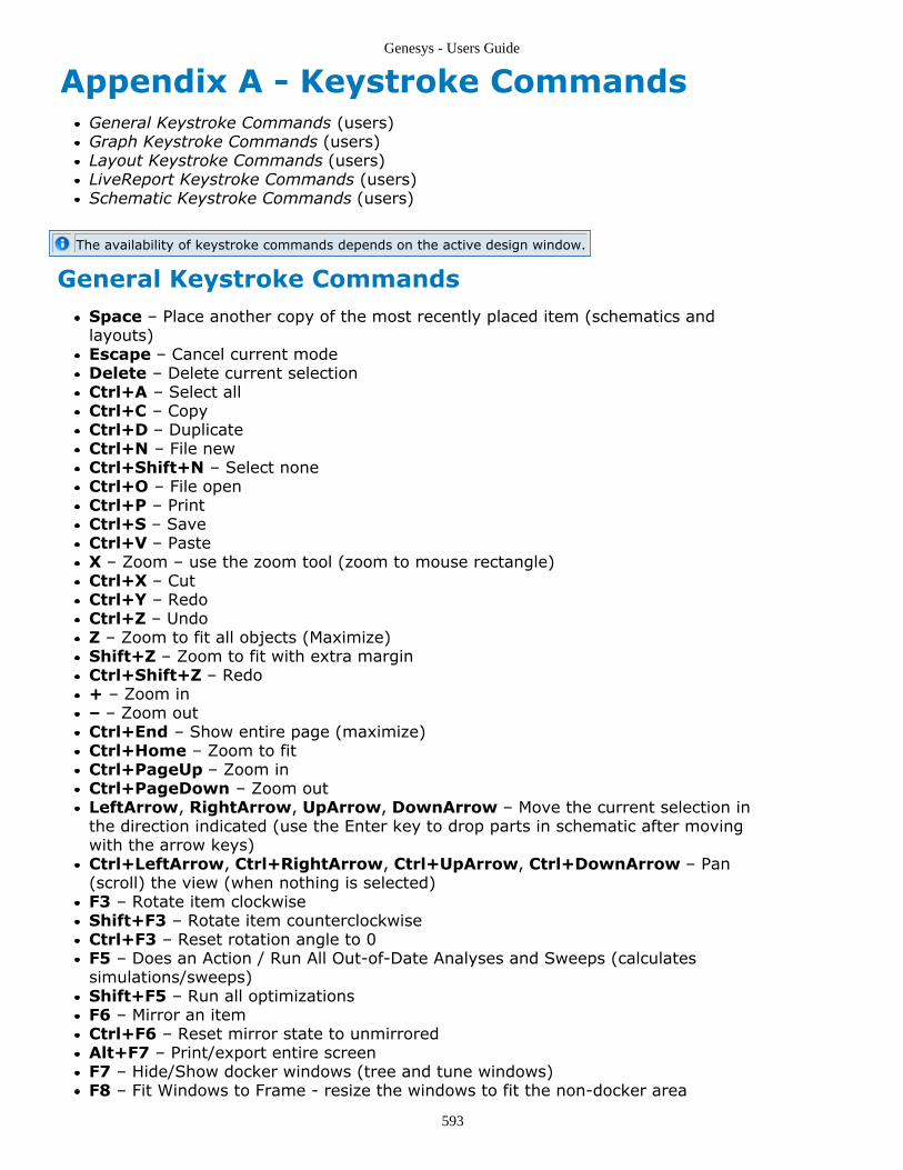
Genesys - Users Guide
593
Appendix A - Keystroke CommandsGeneral Keystroke Commands (users)Graph Keystroke Commands (users)Layout Keystroke Commands (users)LiveReport Keystroke Commands (users)Schematic Keystroke Commands (users)
The availability of keystroke commands depends on the active design window.
General Keystroke CommandsSpace – Place another copy of the most recently placed item (schematics andlayouts)Escape – Cancel current modeDelete – Delete current selectionCtrl+A – Select allCtrl+C – CopyCtrl+D – DuplicateCtrl+N – File newCtrl+Shift+N – Select noneCtrl+O – File openCtrl+P – PrintCtrl+S – SaveCtrl+V – PasteX – Zoom – use the zoom tool (zoom to mouse rectangle)Ctrl+X – CutCtrl+Y – RedoCtrl+Z – UndoZ – Zoom to fit all objects (Maximize)Shift+Z – Zoom to fit with extra marginCtrl+Shift+Z – Redo+ – Zoom in– – Zoom outCtrl+End – Show entire page (maximize)Ctrl+Home – Zoom to fitCtrl+PageUp – Zoom inCtrl+PageDown – Zoom outLeftArrow, RightArrow, UpArrow, DownArrow – Move the current selection inthe direction indicated (use the Enter key to drop parts in schematic after movingwith the arrow keys)Ctrl+LeftArrow, Ctrl+RightArrow, Ctrl+UpArrow, Ctrl+DownArrow – Pan(scroll) the view (when nothing is selected)F3 – Rotate item clockwiseShift+F3 – Rotate item counterclockwiseCtrl+F3 – Reset rotation angle to 0F5 – Does an Action / Run All Out-of-Date Analyses and Sweeps (calculatessimulations/sweeps)Shift+F5 – Run all optimizationsF6 – Mirror an itemCtrl+F6 – Reset mirror state to unmirroredAlt+F7 – Print/export entire screenF7 – Hide/Show docker windows (tree and tune windows)F8 – Fit Windows to Frame - resize the windows to fit the non-docker area

Genesys - Users Guide
594
Ctrl+F8 – Next editorAlt+F8 – Print/export active window
Graph Keystroke CommandsC – Checkpoint – Create a graph checkpoint or remove existing checkpointsF – Favorite – save a graph axis favoriteB – Back – use a graph axis favoriteV – Vertex – Hide / Show vertex symbolsR – Right – Show markers on right / floatingM – Mark – mark all traces with markersL – Legend – hide/show the legendP – Pan – use the pan (scrolling) toolX – Zoom – use the zoom tool (zoom to mouse rectangle)Z – Zoom to fit – Maximize the viewTab – Select the next marker.Shift+Tab – Select the previous marker.Enter – Bring up the Marker Properties window. If no marker is selected, it brings upthe Graph Properties instead.Delete – Delete the currently selected marker.Shift+Delete – Delete all markers (you are asked to confirm the deletion beforedeleting the markers).Arrow Keys – The up, down, left, and right arrow keys have several functions,based on the currently selected marker's style.
Standard Marker – Move the reference frequency left or right on the graph.Peak Marker – Move to the next peak (if any).Valley Marker – Move the marker to the next valley (if any).Bandwidth Marker – Move the relative markers to increase or decrease thebandwidth. This changes the delta values of the child relative markers, so eacharrow key action does not always move the marker by a single data point.Delta Marker – Increase or decrease the relative delta. This changes the dBDown value of the marker, so each arrow key action does not always move themarker by a single data point.
Ctrl+Arrow Keys – Pan (scroll) the chart up, down, left, or right.Shift+Arrow Keys – Move the marker up or down to the next trace on the graph (ifany).Ctrl+Shift+S – Change the current marker's style to Standard.Ctrl+Shift+P – Change the current marker's style to Peak.Ctrl+Shift+V – Change the current marker's style to Valley.Ctrl+Shift+B – Change the current marker's style to Bandwidth.Ctrl+Shift+L – Change the current marker's style to Delta Left.Ctrl+Shift+R – Change the current marker's style to Delta Right.
Layout Keystroke CommandsA – ArcB – Box (rectangle)C – ComponentD – RedrawE – Empower portF – Flip selected line or arcG – GroupL – Line (Wire)O – Toggle orthogonal line modeP – PourShift+P – PolygonR – Toggle pounded (pads or lines)

Genesys - Users Guide
595
Shift+R – Switch to ruler toolT – TextU – UngroupV – ViaShift+W – Wire (line)Z – Zoom to fit0 (Zero) – PadF11 – Show layout preferences
LiveReport Keystroke CommandsA – All Zoom - zoom to pageP – Pan - use the pan (scrolling) toolX – Zoom - use the zoom tool (zoom to mouse rectangle)W – Zoom to WidthZ – Zoom to fit - Maximize the viewTab – switch to next windowShift+Tab – switch to previous window1, 2, 3, 4, 5, ... – switch to nth window (zooms to fit specified window)
Schematic Keystroke CommandsEnter – Bring up part properties or place parts moved using the arrow keysA – Places an ammeter (CURRENT_PROBE)B – BLOCK (two-port)C – CAPQ (capacitor with Q)Shift+C – CAPACITOR (ideal)D – DIODEG – GROUNDI – INPUT PortL – INDQ (inductor with Q)Shift+L – INDUCTOR (ideal)M – MLI_SLIN – BIP_NPNO – OUTPUT portP – Use the Pan (scrolling) toolQ – SQUARE_BLOCK (attached to a design)R – RESISTORS – SIGNAL_GROUNDTEE – Microstrip TV – Voltage TEST_POINTW – 90 degree WIRES (Shift+W for any angle wires)Shift+W – Angled WIREX – Zoom - use the zoom tool (zoom to mouse rectangle)Y – CRYSTALZ – Zoom to show all parts (zoom to fit)Shift+Z – Zoom to show all parts (with extra margin)F4 – Rotate the text origin of part parameters1, 2, 3, ..., 0 – Place 1-port, 2-port, ..., 10-port

Genesys - Users Guide
596
Appendix B - MenusAction Menu (users)Edit Menu (users)Equations Menu (users)File Menu (users)Graph Menu (users)Help Menu (users)Layout Menu (users)LiveReport Menu (users)Notes Menu (users)PartList Menu (users)Schematic Menu (users)Scripts Menu (users)Tools Menu (users)View Menu (users)Window Menu (users)
Action MenuUse this menu to calculate variables or to access the Create Part, Design, or Sourcewizards.
To open: Click the Action button on the menu.
Calculate – Calculate the out-of-date simulations.1.Calculate All Optimizations – Run all the optimizations.2.Revert to Original Settings – Return all tuned variables to their "Original" values.3.Select Tuned Variables – Make any parameter from a master list tunable.4.Create Part Wizard – Run the part creation wizard. Use this to create a new part5.based on existing parts or from scratch by defining the model and symbol for thepart.Design Wizard – Run the design creation wizards. Use this to create Models,6.Symbols, and general Designs.Print Screen – print the current screen.7.
Design MenuDesigns do not have a menu of their own, instead the current tab page menu is displayed(Schematic, PartList, etc.)

Genesys - Users Guide
597
Edit MenuUse this menu to perform basic editing functions, such as undo, redo, cut, paste, copy,and delete.
To open: Click the Edit button.
Undo – Reverse previous editing. Multi-level undo is available in a schematic or1.layout.Redo – Put back changes that were previously reversed with Undo.2.Cut – Copy the selected object and delete it.3.Copy – Copy the selected object. The selection is not deleted.4.Paste – Paste the last copied object into the current schematic, layout, text, etc.5.Delete – Delete the selected object.6.Duplicate – Duplicate the selected object. This is equivalent to a copy-and-paste7.sequence.Mirror – Flip the selected object about its horizontal or vertical axis. Mirror is not8.available for layouts, because it yields backward parts.Rotate – Rotate the selected object by the Part Constrain angle specified in the9.Global Schematic Options window.Bring To Front – Moves the selected item(s) in front of the other items in the10.window.Send To Back – Moves the selected item(s) behind the others.11.Rotate Counterclockwise – Rotate the selected object counterclockwise.12.Select – Display a submenu allowing easy access to commonly used objects13.All – Select all objects in the schematic or layout.14.None – Turn off all selected objects.15.Properties – Open properties for active object.16.Workspace Properties – Open workspace properties.17.
Equations MenuUse this menu to access equations commands.
To open: Click the Script button on the menu.

Genesys - Users Guide
598
Active – When checked, this equation is available for use.1.Auto Calculate – When checked, these equations will recalculate while typing2.
Caution: be careful not to write infinite loops if this option is checked
Show Line Numbers – Shows / hides line numbers in the equations window.3.Show Folding – Shows / hides the folding bar in the equations window (next to line4.numbers). When enabled, the folding bar can be used to expand/contract blocks ofcode, such as if / then / else sections.Equation Wizard – Runs the Equation Wizard.5.Run Equations – Executes the equation block.6.Show Equation Errors – Helps diagnose equation errors.7.Snapshot – Create a dataset with static variables that capture the current state of8.the equation block. Use it save reference variables, such as when the equation blockis dependent on an analysis that gets re-run and you want to keep around old resultsin the workspace.Properties – Shows the Equation's Properties dialog box9.
File MenuUse this menu to open, close, save, or print designs. You can also import or export files,and exit.
To open: Click the File button on the menu.
New – Close the current workspace and open a new workspace. If you select the1.Allow Multiple Open Workspaces option on the General Global Options page, thecurrent workspace remains open.

Genesys - Users Guide
599
Open – Opens a new workspace.2.Close Workspace – Close the current workspace.3.Save – Save the current workspace. If the current file has not been previously4.saved, you will be prompted for a file name.Save As – Save the current workspace into a new file.5.Save All Workspaces – Save all loaded workspaces.6.Page Setup – Select printer and settings.7.Print – Print the active window.8.Export – Display a submenu allowing access to all of the Export options.9.
ASCII Drill List – Export an ASCII (Text) X-Y drill hole list from the currentlayout.Export Schematics to ADS – Export a schematic directly ADS.Bill of Materials – Export a bill of materials from the current layout.Bitmap (Active Window) – Export the active window.Bitmap (Entire Screen) – Export the entire screen, including any applicationsoutside the window.DXF/DWG File – Export a DXF/DWG File from the current layout.GDSII File – Export a GDSII File from the current layout.Gerber File – Export a Gerber File from the current layout. Available formatsare Gerber 274-D and 274-X.HPGL File – Export a HPGL File from the current layout.IFF Schematic File – Export an ADS compatible IFF schematic file.Part Placement List – Export a part placement list from the current layout.S-Parameters – Export a device data file from a simulation.SPICE File – Export a SPICE file from the current schematic.Touchstone File – Export a Touchstone file from the current schematic.XML File – Export the published properties to an XML file.
Import – Display a submenu allowing access to all of the Import commands.10.DXF/DWG File – Import a DXF/DWG File into the current layout using SetLayer Mapping.GDSII File – Import a GDSII File into the current layout using Set LayerMapping.Genesys Netlist –Gerber File – Import a Gerber 274-X File into the current layout.LoadPull Data File – Display a submenu of Load Pull import options.M-File – Import an M-file.Directory of M-Files – Import all M-files in a directoryS-Data file - Import an S Parameter file in Touchstone format.SPICE File – Import a SPICE file.XML – Import an XML file.6.x Model Library – Import a model library that was created in GenesysVersion 6.5B or earlier.Old Genesys S-Data file - For 3+ ports Genesys S-parameters were savedtransposed from the Touchstone standard. Import this old format.CITI File – Import a Common Instrumentation Transfer and Interchange (CITI)file.
Send as Email – Send the current workspace as an email attachment using your11.email program.
Graph MenuThe Graph menu and toolbar appear and disappear on whether or not a graph is theprincipal focus. The work carried out by the menu items or toolbar buttons are common toall types of graphs including accessing a particular graph's Graph Properties (users).Another way to get to Graph Properties is by right-clicking on the graph and selecting iton the pop-up menu.

Genesys - Users Guide
600
Use this menu to specify various graph settings.
To open: Click the Graph button on the menu. (This menu appears only when a graphwindow is active.)
Show Vertex Symbols – Show or hide the vertex symbols on the trace.1.Marker Values On Right -- Place marker values on the right of the graph.2.Show Vertical Marker Lines – Show or hide the vertical marker lines.3.Mark All Traces -- Place markers on all traces.4.Checkpoint -- Remove all current checkpoint traces if there are any. Create one if5.there are none.Marker Properties – Open the Marker Properties window.6.Marker Style – Display a submenu allowing easy access to commonly used marker7.styles.Standard (Fixed Frequency) – Place a maker on the graph at the sport where you8.clicked.Peak – Place a marker at the highest point on the trace.9.Valley – Place a marker at the lowest point on the trace.10.Bandwidth – Placer a marker on the trace to indicate bandwidth.11.Delta (On Left) – Place a marker left of the trace to indicate the relative offset12.specified in the Marker Properties window.Delta (On Right) – Place a marker right of the trace to indicate the relative offset13.specified in the Marker Properties window.Delete Marker – Delete the currently selected marker.14.Delete All Markers – Delete all the markers on the current graph; it prompts15.yes/no before actually deleting the markers.Graph Properties – Open the Graph Properties window.16.
Help MenuUse this menu to check for the latest update, get quick access to the Agilent Web site, orget help.
To open: Click the Help button on the menu.

Genesys - Users Guide
601
Contents – Open the Help contents.1.Index – Open the Help index.2.Keystroke Commands – Open a Help topic containing information about all of the3.keystroke commands.Open Example – Open an example workspace.4.Tutorial Videos – Select and watch a collection of short, helpful videos.5.Update Authorization Information – Open a page where you can start the6.authorization process.Check for Updates – Open a Web page to check for updates.7.Agilent.com – Open the Agilent Web site.8.Technical Support – Open the technical support Web page.9.Web Forums – Open the Web page to access one of the forums.10.Show Start Page – Open the Start page.11.System Information –12.About – Open a page with information about the program.13.
Layout MenuUse this menu to specify drawing modes or change layout properties.
To open: Click the Layout button on the menu. This menu appears only when a layoutwindow is active.

Genesys - Users Guide
602
Center Selected on Page – Center the selected parts on the layout page.1.Connect Selected Parts – Connects the selected parts, by placing them together2.(so that they are touching).Place Footprint Port – If the layout is a footprint, place a port.3.Set Origin – Place the origin on a layout. (The origin is initially placed in the lower4.left corner of the layout.)Step and Repeat – Creates a row/column matrix, by copying the current selection5.and pasting it repeatedly. Use this feature to create rows of evenly spaced pads, DIPpackages, etc.Switch/Move Parts – Used with packages containing parts from more than one6.schematic, to move parts from one schematic to another.Find Part In Schematic – Searches the schematic for currently selected Layout7.component.Show/Hide Layers – Checked Layers (on the popout menu) will be displayed;8.unchecked layers will be hidden.View 3D Geometry – Displays a 3-Dimensional view of your layout. For more9.details, see note below.Hollow Drawing Mode – Emphasize edges of lines, polygons, and other objects.10.Solid Drawing Mode – Use classic opaque fill of lines, polygons, and other objects.11.This is the fastest drawing mode."X-Ray" Drawing Mode – Use semi-transparent fill of lines, polygons, and other12.objects. This technique shows overlapping items best.Enable Adjustable TLines – Allow transmission lines to be resized by dragging13.handles.Measure Distance – Measure the distance between two points.14.Layout Properties – Open the Layout Properties window.15.Parameters – Open the properties window for the selected part.16.
NoteTo see currents or farfield data displayed in a 3D view:
set up a Momentum Analysis to generate desired datarun the anakysisright-click it on the workspace treeselect View 3D Geometry from the menu
LiveReport MenuUse this menu to set LiveReport options. (A LiveReport is a living notebook page thatcollects live views of schematics, graphs, equations, notes, and tables into a single page.)
To open: Click the Schematic button on the menu. This menu appears only when aschematic window is active.
Show Grid – Show or hide the background grid.1.Snap to Grid – Toggles (enables / disables) mouse cursor snap-to-grid (constrains2.mouse coordinates to the grid).Properties – Shows the LiveReport Properties dialog box, which allows you to3.specify settings such as Page Width and Height, Paper Orientation, Margins, Headers,and Footers.

Genesys - Users Guide
603
Notes MenuUse this menu to access Note commands.
To open: Click the Action button on the menu.
Export – Export the Note's text.1.Import – Import text into the note.2.Properties – Shows the Note's Properties dialog box3.
In order for the Note menu to reveal, the Notes page must be the current selected window (either open orminimized) in the Genesys workspace area.
PartList MenuThe PartList has a single item:Properties – Open the Properties window.
Schematic MenuUse this menu to set component and schematic options.
To open: Click the Schematic button on the menu. This menu appears only when aschematic window is active.
Make Components Tunable – Force selected components to be tunable or1.optimizable by adding question marks (?) to the first value of each component. Thisonly adds question marks to part values with a numerical value. If a variable is usedfor a particular value, it is not made tunable.Make Components Fixed – Force selected components to be non-tunable by2.removing any question marks that were added to the first value of each component.This only removes question marks on part values with a numerical value.Add Title Block – Adds a schematic title block to the page, so that the schematic3.can be documented.Center Schematic – Center the schematic on the page.4.

Genesys - Users Guide
604
Fit Page to Schematic – Resize the page to fit all the parts within it. Note that you5.can also change the standard part length in a schematic to have parts shrink to fit aspecific page size.Reapply Auto-Designators – Reassign standardized designators to selected6.components. A designator is a part name like R1 or C3. The Auto-Designator featurebuilds component names by using the appropriate designator prefix (like R for aresistor or C for a capacitor) and appending a unique sequence number to the end.When you use this command, the designators are applied in geometric order, fromleft to right.Renumber Nodes – Renumber all nodes in the schematic, regardless of any7.selection. When you use this commend, the nodes are numbered in geometric order,from left to right. Nodes that connect to a port are set to match the port number (ifthat option is enabled). This is primarily useful before exporting a SPICE file.Bring to Front – Move the selected objects to the front.8.Send to Back – Move the selected objects to the back.9.Keep Connected – Allow wires to remain connected to components as they are10.moved. The ALT key temporarily toggles this function as long as the key is helddown.Show Grid – Show or hide the schematic grid.11.Snap to Grid – Toggles (enables / disables) mouse cursor snap-to-grid (constrains12.mouse coordinates to the grid).Convert Using Advanced TLine – Convert all electrical transmission line parts to13.physical transmission line parts using Advanced TLine (for example, microstrip,stripline, coplanar, or coax). This allows discontinuities to be added and automaticallycompensated for. Also, substrates can be converted from one to another.Schematic Properties – Shows the Schematic Properties dialog box, which allows14.you to specify settings such as Page Width and Height, Title, Company Name, andCompany Address.Edit Selected Part Properties – Shows the Part Properties dialog box, which allows15.you to specify parameters and settings for the selected part.
Scripts MenuUse this menu to access scripting commands.
To open: Click the Script button on the menu.
Copy to Script Processor – Copies the script to the Script Processor window.1.Run – Executes the script.2.Properties – Shows the Script's Properties dialog box3.
The script menu shows only when a script page is present.
To add a script page, use the "New Item" button or Right-Click an existing schematic tab.See images below.

Genesys - Users Guide
605
Tools MenuUse this menu provides access some common design tools or change the global options.
To open: Click the Tools button on the menu.
Equation Measurement Wizard – Open the Equations Measurement wizard. This1.option is available when the Equation window is active.Library Manager – Open the Library Manager window.2.Script Processor – Open the Script Processor window.3.Footprint Editor – Edit layout component footprints.4.
New Footprint – Create a new, blank footprint.

Genesys - Users Guide
606
Load Footprint – Load an existing footprint for editing.Merge Footprint – Adds an additional footprint to the footprint that is currentlybeing edited.Save Footprint – Saves the current footprint into a footprint library. Choose<New Object> to add a new footprint to the library -or- select an existingfootprint to replace.Modify Footprint Library – Allows footprints in a library to be renamed ordeleted.
Options – Open the Global Options window.5.
View MenuUse this menu to adjust the size of your window. This menu can also be use to show orhide docking windows or toolbars.
To open: Click the View button on the menu.
Zoom In – Zoom in on the center of the window.Zoom Out – Zoom out from the center of the window.Zoom Page – Zoom to fit the page.Zoom Maximum – Zoom to fit all objects or traces.Zoom Rectangle – Allow you to draw a rectangle to zoom in on.Part Selector – Show or hide the Part Selector.Error Log – Show or hide the Error Log.Simulation Log – Show or hide the Simulation Log.Workspace Tree – Show or hide the Workspace tree.Advance Windows – Show a secondary list of docking windows.
Equation Debug – Show or hide the Equation Debug window.Library Selector – Show or hide the Library(Design) Selector.Part Selector (2nd copy) – Show or hide a second copy of the Part Selector.Tune – Show or hide the Tune window, which lists and controls tune variables.

Genesys - Users Guide
607
Toolbars – Choose how toolbars are shown.Main – Show or hide the Main toolbar.Show All Object Toolbars – Show toolbars for the active object.Hide All Object Toolbars – Hide toolbars for the active object.
Status Bar – Show or hide the status bar at the bottom of the main window.
Window MenuUse this menu to organize or open a window. You can also use this menu to close all openwindows at the same time.
To open: Click the Window button on the menu.
Tile Horizontal – Tile open windows above each other.1.Tile Vertical – Tile open windows beside each other.2.Cascade – Arrange open windows in an overlapping style.3.Close All – Close all open windows.4.New Window – Open a new design window.5.Tabbed Windows – Switches between tabbed and overlapping document window6.styles.Show Dockers – Show / hide vertical dockers (Tune, Workspace Tree, Part Selector,7.etc.).Fit Windows to Frame – Resizes the open windows to fit the non-docker area.8.Next Editor – Toggle between editor windows (schematics, layouts, equation9.editors).Show All Output Windows – Open all output windows (graphs, tables, variable10.

Genesys - Users Guide
608
viewers).Numbered Window List – A pick-list of all open document windows. Select one to11.make it active (current).

Genesys - Users Guide
609
Appendix C - ToolbarsAnnotation Toolbar (users)Basic Toolbar (users)Coax Toolbar (users)CoPlanar Toolbar (users)Dataset Toolbar (users)Equation Toolbar (users)Graph Toolbar (users)Layout Toolbar (users)Linear Toolbar (users)LiveReport Toolbar (users)Lumped Toolbar (users)Main Toolbar (users)Microstrip Toolbar (users)Nonlinear Toolbar (users)Notes Toolbar (users)Part Groups Toolbar (users)Schematic Toolbar (users)Script Toolbar (users)Slabline Toolbar (users)Spectrasys Toolbar (users)Stripline Toolbar (users)Table Toolbar (users)TLine Toolbar (users)Wave Toolbar (users)
Annotation ToolbarUse this toolbar to add basic drawing objects, such as lines, circles, or arrows, to a designor to modify the selected annotations by changing the color, dashed line style, etc.
To open: Click the Annotation button ( ) from any design window toolbar, e.g.schematic window toolbar.
Select – Select an object.1.Rectangle – Draw a square or rectangle.2.Ellipse – Draw a circle or ellipse.3.Polygon – Draws a filled polygon or unfilled polyline.4.Arrow – Draw a line or arrow. Change the arrow style by selecting a line and picking5.an arrow type from Arrows button menu.Arc – Draw an arc.6.Picture – Insert a picture. Use this annotation to add a company logo to a graph, for7.example. Double-click the new object and select a JPG, GIF, or BMP image file to bedisplayed. To allow all users to see the image, the bitmap file should reside on anetwork server.Text – Place text. Text has a number of settings. Double-click a text annotation to8.set the horizontal and vertical justification (text alignment). The name of the textitem can be changed and shown on-screen, which simplifies building a schematic titleblock.Text Balloon – Draw a text balloon. This annotation has a "tail" which can be9.

Genesys - Users Guide
610
anchored to a data point on a graph, to the page, or not anchored (using the right-button menu).Button – Draw a user button (widget). This annotation can be "clicked" to run a10.custom script, which is specified by double-clicking the outer EDGE of the buttoncontrol. The middle of the button runs the script.Slider – Draw a slider control (widget). This annotation is linked to a tunable11.parameter and functions much like the Tuning Window.Fill Color – Set the fill color. Use the 3 color buttons to change the colors of the12.selected annotations. New annotations will be created using the current colors. Thebottom-right color swatch (with a diagonal slash) is transparent, which specifies anunfilled object.Line Color – Set the line color. The bottom-right color swatch (with a diagonal slash)13.is transparent, which specifies a object with no outline.Text Color – Set the text color.14.Line Thickness – Set the width of borders and lines.15.Line Style – Set the drawing style of borders and lines (dash pattern, etc.).16.Arrows – Set the arrow style of lines.17.Properties – Display the properties window for the selected part.18.
Basic ToolbarUse this toolbar to place basic components.
To open: Click the Basic button on the Schematic Toolbar.
Draw a 90-degree Connection Line (W)
90-degree Connection Line (W)
Draw a Angled Connection Line (Shift+W)
Connection Line (Shift+W)
Place an Input (I)
Input: Standard (*INP) (part)Input: AC Power (PAC) (part)Input: DC Voltage (part)Input: DC Current (part)Input: AC Voltage (part)Input: AC Current (part)Input: Pulsed Voltage (part)Input: Pulsed Current (part)Input: Custom Voltage Waveform (part)Input: Custom Current Waveform (part)Input: AC Power (PAC) with uniform Noise (part)Input: Noise Power (uniform) (part)Input:AC Power (PAC) with Custom Noise (part)Input: Custom Noise Power (part)
Place an Output (O)

Genesys - Users Guide
611
Output (O) (part)
Place a Ground (G)
Ground (G) (part)
Place a Signal Ground/DC Source (S)
Signal Ground/DC Source (S) (part)
Place a Source, Current Probe or Test Point
Source: AC Power (PAC) (part)Source: DC Voltage (part)Source: DC Current (part)Source: AC Voltage (part)Source: AC Current (part)Source: Pulsed Voltage (part)Source: Pulsed Current (part)Source: Custom Voltage Waveform (part)Source: Custom Current Waveform (part)Source: Noise Voltage (part)Source: Noise Current (part)Current Probe (Ammeter) (part)Voltage Test Point (part)Oscillator Port (part)
Place a Reused Schematic
Subcircuit 1-PortSubcircuit 2-PortSubcircuit 3-PortSubcircuit 4-PortSubcircuit 5-PortSubcircuit 6-PortSubcircuit 7-PortSubcircuit 8-PortSubcircuit 9-PortMore Subcircuit Models...
Coax ToolbarUse this toolbar to insert Coaxial parts in the schematic.
To open: Click the Coax button on the Schematic Toolbar.
CLI: Coaxial Line
Coaxial Line (CLI) (part)Coaxial Cable (part)RG6 Cable (part)RG8 Cable (part)

Genesys - Users Guide
612
RG9 Cable (part)RG58 Cable (part)RG59 Cable (part)RG214 Cable (part)
CLI4: 4 - Terminal Coaxial Line
CLI4: 4 - Terminal Coaxial Line (part)
CEN: Coaxial End Effect
CEN: Coaxial End Effect (part)
CGA: Coaxial Gap
CGA: Coaxial Gap (part)
CSQLI,CSQLX: Square Coaxial Lines
Square Coaxial Line (Round Inner Conductor) (part)Square Coaxial Line (Square Inner Conductor) (part)
CST: Coaxial Step
CST: Coaxial Step (part)
Co-Planar ToolbarUse this toolbar to place co-planar parts.
To open: Click the Co-Planar button on the Schematic Toolbar.
CPW: Coplanar Line
CPW: Coplanar Line (part)
CPWG: Coplanar Line with Ground
CPWG: Coplanar Line with Ground (part)
GPWCGAP: Coplanar Line with Gap
GPWCGAP: Coplanar Line with Gap (part)
Dataset ToolbarUse this toolbar to interact with the active Dataset (users) and adjust its settings.

Genesys - Users Guide
613
Properties - Brings up the Dataset Properties dialog.1.Save - Export/save the dataset to a file.2.
Equations ToolbarUse this toolbar to change the Equation window display options and debug your equations.This toolbar automatically displays when you have an Equation window active.
The icons are:
Show or hide the Line Numbers margin
Turn autocalculate on/off
Bring up the Equation Wizard
Display Errors for this set of equations
Go - run the equations, or continue on from a breakpoint (F5 or Ctrl_G)
Stop - stop debugging (abort execution). This button is only enabled whilebreakpointed.
Step Into - step inside a function and break at the first line of execution in the function(F11). This button is only enabled while breakpointed.
Step Over - execute statements on the current line (F10). This button is only enabledwhile breakpointed.
Step Out - run until the current function ends, then break at the next line (the caller)(Shift_F11). If there is no function call at the current line, or the equation processorcannot step into the function, then all statements on the current line are simply executed.This button is only enabled while breakpointed.
Add or Remove a breakpoint from the current line (F9 or Ctrl_B)
Toggle all existing breakpoints to either the "enabled" or "disabled" state
Graph ToolbarUse the toolbar for Graph functions.
To open: Open a graph window.
Annotation – Display the Annotation Toolbar toolbar.1.Eye – Hide/Show graph traces in a pulldown menu2.Graph Properties – Display the Graph Properties window.3.Select – Select an object.4.Pan – use the Pan tool to pan the graph (left-right for rectangular graphs, free for5.polar and smith charts).Zoom – zoom in on a selected part of the graph.6.Checkpoint – Add a checkpoint if there is none. Remove all current checkpoint7.traces if there are anyAdd Axis Favorite – Save the current axis settings into the Axis Favorite list.8.Zoom to Page – Zoom the graph data attractively to fit the page.9.Maximize – Zoom the graph data exactly to fit the page..10.Use Axis Favorite – Set the axis settings to the last favorite in the list. Click again11.

Genesys - Users Guide
614
to cycle through the axis favorites.Toggle Vertex Symbols – Show or hide trace vertex symbols (large dots on traces).12.Marker Values On Right – Place marker text in right margin of graph, or inline in13.graph.Mark All Traces – Mark all traces on the graph.14.Toggle Vertical Marker Lines – Show or hide dashed vertical marker lines at every15.marker position.Delete Marker – Delete the selected marker.16.Delete all Markers – Delete all markers on the current graph.17.Marker Properties – Display the Marker Properties window.18.Standard Marker – drop a standard marker or convert a selected marker to19.standard.Peak Marker – Change marker style to Peak.20.Valley Marker – Change marker style to Valley.21.Bandwidth Marker – Change marker style to Bandwidth and insert two Delta22.markers.Delta Marker (On Right) – Place a new Delta marker on the left side of the23.selected marker.Delta Marker (On Left) – Place a new Delta marker on the right side of the selected24.marker.
Layout ToolbarUse the toolbar to place components and edit in Layout. The Layout toolbar automaticallydisplays when a Layout is active. Note that many of these buttons are tool specific; theywill only appear when it is appropriate.
To open: Open a layout window.
Select – Select an object.1.Line – Draw a line.2.Rectangle – Draw a rectangle.3.Arc – Draw an arc.4.Polygon – Draw a polygon.5.Port – Place an EMport in the layout window. (In the Footprint editor, this button6.places a footprint port.)Component – Place a component footprint from the library.7.Text – Place text.8.Viahole – Draw a viahole, including pads.9.Pad – Draw a round, square, or wagonwheel pad.10.View 3D Geometry – Displays a 3-Dimensional view of your layout. For more11.details, see note below.Ruler – Measure the distance between two specified points.12.Layer – Displays layer name.13.Line Width – Displays line width.14.Round End – Switch to line round ends.15.Square End – Switch to line square ends.16.Ambiguous Ends – Revert multiple lines (within a selection) to back to the original17.line endings.Square – Change pad type to wagon wheel.18.Wagon Wheel – Change pad type to circle.19.

Genesys - Users Guide
615
Circle – Change pad type to square.20.Unpour – Unpour polygon.21.Pour – Pour/repour the polygon.22.Convert Pour – Convert pour to polygon.23.Group Objects – Place the selected objects into a group.24.Ungroup Objects – Ungroup the objects in the selection.25.Save as Footprint – Save the selection as a footprint.26.Mirror – Flip by 180 degrees along an axis (toggles between X and Y axis during27.use).Scissors – Cut a hole in the polygon.28.Footprint to Group – Convert footprint to group, to allow editing.29.
NoteTo see currents or farfield data displayed in a 3D view:
set up a Momentum Analysis to generate desired datarun the anakysisright-click it on the workspace treeselect View 3D Geometry from the menu
Linear ToolbarUse this toolbar to insert linear parts.
To open: Click the Linear button on the Schematic Toolbar.
Each of the n-Port blocks has an option to load an s-parameter file (from the item'sproperties, available by double-clicking it in schematic view)
1-Port (S-Parameter)
1-Port (S-Param w/1 Terminal) (part)1-Port (S-Param w/2 Terminal) (part)
2-Port (S-Parameter)
2-Port (S-Param w/2 Terminal) (part)2-Port (S-Param w/BIP_NPN) (part)2-Port (S-Param w/BIP_PNP) (part)2-Port (S-Param w/N_FET) (part)2-Port (S-Param w/P_FET) (part)2-Port (S-Param w/BLOCK and Gnd) (part)2-Port (S-Param w/Generic and Gnd) (part)Manual ABCD-Parameters (BLOCK) (part)Manual S-Parameters (BLOCK) (part)
Subcircuit (N-Port)
Subcircuit (w/NET2) (part)Subcircuit (w/2-PortNoGnd) (part)
Dataset (S-Parameter N-Port)

Genesys - Users Guide
616
Dataset 1-Port (S-Param) (part)Dataset 2-Port (S-Param) (part)
Multi-Port (S-Parameter)
3-Port Data File (S-Param) (part)4-Port Data File (S-Param) (part)5-Port Data File (S-Param) (part)6-Port Data File (S-Param) (part)7-Port Data File (S-Param) (part)8-Port Data File (S-Param) (part)9-Port Data File (S-Param) (part)10-Port Data File (S-Param) (part)More File (S-Param) models...
FET Models
FET (S-Param w/N_FET) (part)FET (S-Param w/P_FET) (part)FET (N_FET) (part)FET (P_FET) (part)
Bipolar Transistor
Bipolar (S-Param w/BIP_NPN) (part)Bipolar (S-Param w/BIP_PNP) (part)Bipolar (BIP_NPN) (part)Bipolar (BIP_PNP) (part)
Negation /1 or 2 Port
Negation (NEG1) (part)Negation (NEG2) (part)
Current Controlled Current Source
Current Controlled Current Source (part)
Current Controlled Voltage Source
Current Controlled Voltage Source (part)
PIN Diode
PIN Diode (part)
Op Amp
Op Amp (part)
Voltage Controlled Current Source
Voltage Controlled Current Source (part)

Genesys - Users Guide
617
Voltage Controlled Voltage Source
Voltage Controlled Voltage Source (part)
Gyrator
Gyrator (part)
LiveReport ToolbarUse this toolbar to change the LiveReport and adjust its settings. The LiveReport toolbarautomatically displays when you have a LiveReport active.
Annotation – Show/Hide the Annotation Toolbar.1.Arrange – Brings up the Arrange Views dialog box, which repositions all the sub-2.objects.Eye – Use this pull down menu to turn on/off text displays such as Titles, Headers,3.Footers, etc. on the LiveReport.Grid Snap – enable/disable the grid snap4.Select – Use the select tool to select views or annotations..5.Pan – Use the pan (scrolling) tool to pan the schematic around (press the tool button6.and drag the LiveReport).Zoom – Use the zoom tool to zoom into a rectangular region of the LiveReport (press7.the tool button and drag a rectangle).Zoom to Page – Zoom to fit the page.8.Zoom to Fit Selection – Zoom to fit the currently selected objects.9.Zoom to Fit All (Maximize) – Zoom to fit all objects.10.Properties – Opens the LiveReport properties dialog box.11.
Lumped ToolbarUse this toolbar to place lumped parts.
To open: Click the Lumped button on the Schematic Toolbar.
Resistor (R)
Resistor (R) (part)
Capacitor (C)
Capacitor (C) (part)
Inductor (L)
Inductor (L) (part)
Physical Inductors

Genesys - Users Guide
618
Air core inductor (AIRIND1) (part)Inductor with Q (INDQ) (part)Spiral inductor (SPIND) (part)Toroidal core inductor (TORIND) (part)
Ideal parts
Ideal Gain Block (GAIN) (part)Ideal Impedance Inverter (INV) (part)Ideal Isolator (ISOLATOR) (part)Ideal Phase Shift (PHASE) (part)Ideal Three Port Circulator (CIR3) (part)Ideal Time Delay Block (DELAY) (part)
Antenna parts
DIPOLE Antenna (part)MONOPOLE Antenna (part)
Mutually Coupled Inductors
Two Mutually Coupled Inductors (part)2 Mutually Coupled Coils (part)3 Mutually Coupled Coils (part)4 Mutually Coupled Coils (part)5 Mutually Coupled Coils (part)6 Mutually Coupled Coils (part)7 Mutually Coupled Coils (part)8 Mutually Coupled Coils (part)9 Mutually Coupled Coils (part)10 Mutually Coupled Coils (part)
Ideal Transformer
Transformer (part)Center-Tapped Transformer (part)
Thin Film Resistor/Capacitor
Thin film capacitor (part)Thin film resistor (part)
Lumped part Networks
Parallel L-C Resonator: Enter: f,C (PFC) (part)Parallel L-C Resonator: Enter: f,L (PFL) (part)Parallel Network: L-C (PLC) (part)Parallel Network: R-L (PRL) (part)Parallel Network: R-C (PRC)Parallel Network: R-L-C (PRX) (part)Series L-C Resonator: Enter: f,C (SFC) (part)Series L-C Resonator: Enter: f,L (SFL) (part)Series Network: L-C (SLC) (part)Series Network: R-L (SRL) (part)

Genesys - Users Guide
619
Series Network: R-C (SRC) (part)Series Network: R-L-C (SRX) (part)Frequency-Independent Impedance (IMP) (part)
Crystal (Y)
Crystal (Y) (part)
Main ToolbarUse this toolbar for global functions, like File Save, Print, and Undo.
To open: Click View on the menu and select Main from the Tools menu.
Start Page – Create a new workspace.1.Open – Open an existing document.2.Save – Save the active document.3.Cut – Cut the selection to the clipboard.4.Copy – Copy the selection to the clipboard.5.Paste – Paste the contents of the clipboard.6.Undo – Undo the last action. Available only for schematics and layouts.7.Redo – Redo the previously undone action. Available only for schematics and8.layouts.Print – Print the active window.9.Help – Open the Help file.10.Docker View Menu – Drop down menu to allow dockers to be toggled hidden or11.shown.Hide/Show Dockers – Hide or show the Tree and Tune windows. (Hide them for12.more work area).Fit Windows To Frame – Resize all of the object windows to fit into the frame.13.Run Analysis – Run one or more analyses (calculate simulations).14.
When the active document window is a design/schematic and there is only oneanalysis associated with it, the analysis will be run.If there are several associated analyses then a list containing all the associatedanalyses (and evaluations) will be displayed, so that the appropriate one may beselected.If no design/schematic is active, or the drop-down arrow to the right of thebutton is clicked, a list containing all the analyses (and evaluations) of theworkspace will be displayed, along with options to run all the out-of-dateanalyses or every analysis in the workspace.
Stop Analyses – The button is shown instead of the Run Analysis button when15.any analysis or Evaluation is currently running. Click the button to stop the runningAnalyses / Evaluations.
The drop-down on the right side of the button displays options to Show or Hidethe Status Window and to Stop Running Analyses/Evaluations.
Errors Window – Open the Errors window.16.
Microstrip ToolbarUse this toolbar to place microstrip parts.
To open: Click the Microstrip button on the Schematic Toolbar.

Genesys - Users Guide
620
MLI: Microstrip Line (Shift+M)
MLI: Microstrip Line (Shift+M) (part)
MCP, MCN4A: 2 Microstrip Coupled Lines
2 Symmetrical Coupled Microstrip Lines (MCP) (part)2 Asymmetrical Coupled Microstrip Lines (MCN4A) (part)
MCN: Multiple Coupled Microstrip Lines
3 Coupled Microstrip Lines (MCN6) (part)4 Coupled Microstrip Lines (MCN8) (part)5 Coupled Microstrip Lines (MCN10) (part)6 Coupled Microstrip Lines (MCN12) (part)7 Coupled Microstrip Lines (MCN14) (part)8 Coupled Microstrip Lines (MCN16)9 Coupled Microstrip Lines (MCN18) (part)10 Coupled Microstrip Lines (MCN20) (part)More`MCN`models... (part)
Inverted/Suspended Microstrip
Suspended Microstrip (MSUS) (part)Inverted Microstrip (MINV) (part)
MBN, MBN3: Microstrip Bends
Bend: Square or Chamfered (MBN) (part)Bend: Optimal Miter (MBN3) (part)Bend: Arbitrary Angle (MBNA) (part)
MCR: Microstrip Cross (Shift+X)
MCR: Microstrip Cross (Shift+X) (part)
MCURVE: Curved Microstrip Line
MCURVE: Curved Microstrip Line (part)
MEN: Microstrip End Effect (Shift+E)
MEN: Microstrip End Effect (Shift+E) (part)
MTE: Microstrip Tee (Shift+T)
MTE: Microstrip Tee (Shift+T) (part)
MGA: Microstrip Gap (Shift+G)

Genesys - Users Guide
621
MGA: Microstrip Gap (Shift+G) (part)
Microstrip Capacitor and Inductors
Interdigital Capacitor (MIDCAP)\tShift+C (part)Spiral Inductor (MSPIND)\tShift+L (part)Rectangular Inductor (MRIND) (part)
Lange Coupler
Lange Coupler, 4 lines (MLANG)Lange Coupler, 6 lines (MLANG6) (part)Lange Coupler, 8 lines (MLANG8) (part)
MST: Microstrip Step (Shift+S)
MST: Microstrip Step (Shift+S) (part)
MTAPER: Microstrip Tapered Line
MTAPER: Microstrip Tapered Line (part)
MRS: Microstrip Radial Stub (Shift+R)
MRS: Microstrip Radial Stub (Shift+R) (part)
MVH: Microstrip Via Hole (Shift+V)
MVH: Microstrip Via Hole (Shift+V) (part)
Nonlinear ToolbarUse this toolbar to place non-linear parts.
To open: Click the Nonlinear button on the Schematic Toolbar.
Nonlinear FETs
Angelov N-Channel (sim)Curtice2 Quadratic N-Channel (part)Curtice2a Advanced Quadratic N-Channel (sim)Curtice3 Cubic N-Channel (part)Parker-Skellern N-Channel (sim)Statz N-Channel (part)TOM N-Channel (part)TOM2 N-Channel (part)TOM3 N-Channel (sim)Angelov P-Channel (sim)Curtice2 Quadratic P-Channel (part)Curtice2a Advanced Quadratic P-Channel (sim)Curtice3 Cubic P-Channel (part)

Genesys - Users Guide
622
Statz P-Channel (part)TOM P-Channel (part)TOM2 P-Channel (part)TOM3 P-Channel (sim)JFET N-Channel (part)JFET P-Channel (part)JFET2 N-Channel (part)JFET2 P-Channel (part)
Nonlinear MOSFETs
MOS1 N-Channel (part)MOS1 P-Channel (part)MOS2 N-Channel (part)MOS2 P-Channel (part)MOS3 N-Channel (part)MOS3 P-Channel (part)MOS9 N-Channel (sim)MOS9 P-Channel (sim)BSIM1 N-Channel (part)BSIM1 P-Channel (part)BSIM2 N-Channel (part)BSIM2 P-Channel (part)BSIM3 N-Channel (part)BSIM3 P-Channel (part)BSIM4 N-Channel (sim)BSIM4 P-Channel (sim)EKV N-Channel (sim)EKV P-Channel (sim)LDMOS MET Model N-Channel (part)LDMOS MET Model P-Channel (part)TFT_ASIA2 N-Channel (sim)TFT_ASIA2 P-Channel (sim)TFT N-Channel (sim)TFT P-Channel (sim)
Nonlinear BJTs
NPN Bipolar Gummel-Poon (BIPNPN) (part)NPN Bipolar Gummel-Poon with Substrate Node (BIPNPN4) (part)NPN Bipolar VBIC (VBICNPN) (part)NPN Bipolar VBIC with Substrate Node (VBICNPN4) (part)NPN Bipolar VBIC with Substrate and Temp. Nodes (VBICNPN5) (part)NPN Bipolar MEXTRAM (MEXTRAM_NPN) (sim)NPN Bipolar MEXTRAM with Substrate Node (MEXTRAM_NPN4) (sim)NPN Bipolar MEXTRAM with Substrate and Temp. Nodes (MEXTRAM_NPN5) (sim)PNP Bipolar Gummel-Poon (BIPPNP) (part)PNP Bipolar Gummel-Poon with Substrate Node (BIPPNP4) (part)PNP Bipolar VBIC (VBICNPN) (part)PNP Bipolar VBIC with Substrate node (VBICNPN4) (part)PNP Bipolar VBIC with Substrate and Temp. Nodes (VBICPNP5) (part)PNP Bipolar MEXTRAM (MEXTRAM_PNP) (sim)PNP Bipolar MEXTRAM with Substrate Node (MEXTRAM_PNP4) (sim)PNP Bipolar MEXTRAM with Substrate and Temp. Nodes (MEXTRAM_PNP5) (sim)

Genesys - Users Guide
623
Nonlinear Power Sources
Current-Controlled Current Source (part)Current-Controlled Voltage Source (part)Voltage-Controlled Current Source (part)Voltage-Controlled Voltage Source (part)
X-Parameters
X-Parameters Part (part)
Nonlinear Diode (D)
Standard Nonlinear Diode (part)
Notes ToolbarUse this toolbar to edit/modify the Note its text settings. The Notes toolbar automaticallydisplays when you have an active Note.
Font - select a font for the selection or for typing1.Size - select a font size in html units (3 = average) for the selection or typing2.Style - click the pulldown to pick from standard html styles3.Bold - embolden selected characters4.Italic - italicize selected characters5.Underline - underline selected characters6.Color - select font color7.Number - number the selected paragraphs8.Bullet - bullet the selected paragraphs9.Exdent - exdent a paragraph (reduce indent)10.Indent - indent a paragraph11.Left Justify - left justify the paragraph12.Center Justify - center justify the paragraph13.Right Justify - right justify the paragraph14.Image - Insert a picture into the notes. This picture is specified by a URL.15.Absolute - position part as absolute16.Static - position part as static17.Hyperlink - add a hyperlink (this is currently disabled)18.
Part Groups ToolbarUse this toolbar to bring up sub-toolbars with palettes of parts on them. This toolbar mayautomatically display when you have a schematic active or use the Schematic Toolbar toshow it.
Basic (users) - Bring up the basic toolbar, which contains ports and sources.1.Lumped (users) - Open or close the Lumped Toolbar, which contains lumped parts.2.Linear (users) - Open or close the Linear Toolbar, which contains component3.models (such as diodes and op-amps).

Genesys - Users Guide
624
Non-Linear (users) - Open or close the Nonlinear Toolbar, which contains nonlinear4.models (such as transistors and diodes).System (users) - Open or close the System Toolbar, which contains RF system5.models.T-Line (users) - Open or close the T-Line Toolbar, which contains ideal transmission6.line models.Coax (users) - Open or close the Coax Toolbar, which contains physical coaxial line7.models.Microstrip (users) - Open or close the Microstrip Toolbar, which contains physical8.microstrip line and discontinuity models.Slabline (users) - Open or close the Slabline Toolbar, which contains physical9.slabline models.Stripline (users) - Open or close the Stripline Toolbar, which contains physical10.stripline line and discontinuity models.Co-Planar (users) - Open or close the Coplanar Toolbar, which contains physical11.coplanar line and discontinuity models.Wave (users) - Open or close the Waveguide Toolbar, which contains rectangular12.waveguide and waveguide-to-TEM adapter models.
Schematic ToolbarUse this toolbar to change a schematic or to bring up another toolbar with commonly usedparts.
OR
Run - Runs the analyses.1.Part Group - Show/Hide the part group toolbar.2.Annotation - Show/Hide the Annotation toolbar.3.Part Selector - Show/Hide the Part Selector.4.Eye - Use this pull down menu to turn on/off text displays such as Part Parameters,5.Net Names, etc. on the schematic.Keep Connect - Enable/disable automatic line connections when dragging parts.6.Grid Snap - Enable/disable the grid snap.7.Select - Use the select tool to select parts or annotations.8.Pan - Use the pan tool to pan the schematic around. Press the tool and drag the9.schematic.Zoom - Use the zoom tool to zoom into a rectangular region of the schematic.10.Line - Use the line tool to draw horizontal, vertical or right angled line connections.11.Angled Line - Use the angled line tool to draw line connections of any orientation.12.Zoom to Page - Zoom to fit the page.13.Zoom to Fit Selection - Zoom to fit the currently selected parts/objects on a14.schematic.Zoom to Fit All - Zoom to fit all object.15.Tune - Make the selected parts tunable or fixed.16.Disable to short - Disable/enable the selected parts and simulate them as short17.circuit.Disable to open - Disable/enable the selected parts and simulate them as an open18.circuit.

Genesys - Users Guide
625
Rotate - Rotate the selected parts by 90 degrees.19.Mirror - Mirror the selected parts.20.Open Model or Symbol - Open part models/symbols. For a single part, this button21.can open its model/symbol library.
Script ToolbarUse this toolbar to interact with the active Script and adjust its settings.
Line Numbers – Hide/Show line numbers on the display.1.Script Processor – Hide/Show the script processor window.2.Copy – copy the script to the script processor.3.Run – copy the script to the script processor and run it.4.
Slabline ToolbarUse this toolbar to place Slabline components.
To open: Click the Slabline button on the Schematic Toolbar.
RLI: Single Slabline
RLI: Single Slabline (part)
RCP: 2 Coupled Slablines
RCP: 2 Coupled Slablines (part)
RCN: Multiple Coupled Slablines
3 Coupled Slablines (RCN6) (part)4 Coupled Slablines (RCN8) (part)5 Coupled Slablines (RCN10) (part)6 Coupled Slablines (RCN12) (part)7 Coupled Slablines (RCN14) (part)8 Coupled Slablines (RCN16) (part)9 Coupled Slablines (RCN18) (part)10 Coupled Slablines (RCN20) (part)More`RCN`models...
Spectrasys ToolbarUse this toolbar to place system parts.
To open: Click the System button on the Schematic Toolbar.

Genesys - Users Guide
626
RF Amplifiers
RF Amplifier - 2nd 3rd Order (part)RF Amplifier - High Order (part)Variable Gain Amplifier (part)
RF Mixers
Basic Mixer (part)Double Balanced Mixer (part)Table Mixer (part)
Attenuators
Attenuator (part)DC Controlled Attenuator (part)Frequency Dependent Attenuator (part)Variable Attenuator (part)
Sources
Multi Source (part)CW Source (part)CW Source with PhaseNoise (part)Wideband Source (part)Multicarrier Source (part)Intermod Source (part)Receiver Intermod Source (part)Continuous Frequency Source (part)Noise Source (part)
Splitters/Combiners
2 Way 0 Degree Splitter/Combiner (part)2 Way 90 Degree Splitter / Combiner (part)2 Way 180 Degree Splitter / Combiner (part)3 Way 0 Degree Splitter / Combiner (part)4 Way 0 Degree Splitter / Combiner (part)5 Way 0 Degree Splitter / Combiner (part)6 Way 0 Degree Splitter / Combiner (part)8 Way 0 Degree Splitter / Combiner (part)9 Way 0 Degree Splitter / Combiner (part)10 Way 0 Degree Splitter / Combiner (part)12 Way 0 Degree Splitter / Combiner (part)16 Way 0 Degree Splitter / Combiner (part)24 Way 0 Degree Splitter / Combiner (part)48 Way 0 Degree Splitter / Combiner (part)
RF Switches
Switch - SPST (part)Switch - SPDT (part)Switch - SP3T (part)Switch - SP4T (part)

Genesys - Users Guide
627
Switch - SP5T (part)Switch - SP6T (part)Switch - SP7T (part)Switch - SP8T (part)Switch - SP9T (part)Switch - SP10T (part)Switch - SP11T (part)Switch - SP12T (part)Switch - SP13T (part)Switch - SP14T (part)Switch - SP15T (part)Switch - SP16T (part)Switch - SP17T (part)Switch - SP18T (part)Switch - SP19T (part)Switch - SP20T (part)
Frequency Multiplier
Frequency Multiplier (part)Frequency Divider (part)Digital Frequency Divider (part)
Analog / Digital Converters
Analog / Digital Converters (part)
Lowpass Filters
Lowpass Butterworth Filter (part)Lowpass Bessel Filter (part)Lowpass Chebyshev Filter (part)Lowpass Elliptic Filter (part)Lowpass Pole Zero Filter (part)
Bandpass Filters
Bandpass Butterworth Filter (part)Bandpass Bessel Filter (part)Bandpass Chebyshev Filter (part)Bandpass Elliptic Filter (part)Bandpass Pole Zero Filter (part)
Highpass Filters
Highpass Butterworth Filter (part)Highpass Bessel Filter (part)Highpass Chebyshev Filter (part)Highpass Elliptic Filter (part)Highpass Pole Zero Filter (part)
Bandstop Filters
Bandstop Butterworth Filter (part)
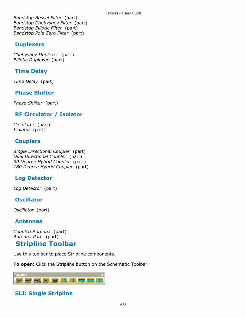
Genesys - Users Guide
628
Bandstop Bessel Filter (part)Bandstop Chebyshev Filter (part)Bandstop Elliptic Filter (part)Bandstop Pole Zero Filter (part)
Duplexers
Chebyshev Duplexer (part)Elliptic Duplexer (part)
Time Delay
Time Delay (part)
Phase Shifter
Phase Shifter (part)
RF Circulator / Isolator
Circulator (part)Isolator (part)
Couplers
Single Directional Coupler (part)Dual Directional Coupler (part)90 Degree Hybrid Coupler (part)180 Degree Hybrid Coupler (part)
Log Detector
Log Detector (part)
Oscillator
Oscillator (part)
Antennas
Coupled Antenna (part)Antenna Path (part)
Stripline ToolbarUse this toolbar to place Stripline components.
To open: Click the Stripline button on the Schematic Toolbar.
SLI: Single Stripline

Genesys - Users Guide
629
SLI: Single Stripline (part)
SCP: 2 Coupled Striplines
SCP: 2 Coupled Striplines (part)
SCN: Multiple Coupled Striplines
3 Coupled Striplines (SCN6) (part)4 Coupled Striplines (SCN8) (part)5 Coupled Striplines (SCN10) (part)6 Coupled Striplines (SCN12) (part)7 Coupled Striplines (SCN14) (part)8 Coupled Striplines (SCN16) (part)9 Coupled Striplines (SCN18) (part)10 Coupled Striplines (SCN20) (part)More`SCN`models...
SLIO: Offset Stripline
SLIO: Offset Stripline (part)
SBCP: Offset Coupled Striplines
SBCP: Offset Coupled Striplines (part)
SBN: Stripline Bend
SBN: Stripline Bend (part)
SEN: Stripline End Effect
SEN: Stripline End Effect (part)
STE: Stripline Tee
STE: Stripline Tee (part)
SGA: Stripline Gap
SGA: Stripline Gap (part)
SSP: Stripline Step
SSP: Stripline Step (part)
Table ToolbarUse this toolbar to interact with the active Table and adjust its settings.
Properties - Bring up the properties dialog.1.

Genesys - Users Guide
630
Save - export/save the table to a file.2.
See Also
Tables (users)
T-Line ToolbarUse this toolbar to place transmission line components.
To open: Click the T-Line button on the Schematic Toolbar.
TLE: Transmission Line
TLE: Transmission Line (part)
TLE4: 4 - Terminal Transmission Line
TLE4: 4 - Terminal Transmission Line (part)
TLP: Physical Transmission Line
TLP: Physical Transmission Line (part)
TLP4: 4 - Terminal Physical Transmission Line
Physical transmission line (part)Open 4 Terminal Stub (part)Shorted 4 Terminal Stub (part)
CPL: 2 Coupled Transmission Lines
CPL: 2 Coupled Transmission Lines (part)
CPNx: Multiple Coupled Line Models
3 Coupled T-Lines (CPN6) (part)4 Coupled T-Lines (CPN8) (part)5 Coupled T-Lines (CPN10) (part)6 Coupled T-Lines (CPN12) (part)7 Coupled T-Lines (CPN14) (part)8 Coupled T-Lines (CPN16) (part)9 Coupled T-Lines (CPN18) (part)10 Coupled T-Lines (CPN20) (part)More`CPN`models...
RIBBON: Ribbon Wire
RIBBON: Ribbon Wire (part)
RLGC: Ideal Distributed Line Models

Genesys - Users Guide
631
Distributed RC T-Line (RCLIN) (part)Distortionless TEM T-Line (TLRLDC) (part)Uniform TEM T-Line (TLRLGC) (part)Exponential TEM T-Line (TLX) (part)
TRFRUTH: Ruthroff Transformer
TRFRUTH: Ruthroff Transformer (part)
WIRE: Round Wire
WIRE: Round Wire (part)
Wave ToolbarUse this toolbar to place waveguide components.
To open: Click the Wave button on the Schematic Toolbar.
WAD: Waveguide Adapter
WAD: Waveguide Adapter (part)
WLI: Rectangular Waveguide
WLI: Rectangular Waveguide (part)